
NBER WORKING PAPER SERIES
OPTIMAL EXPECTATIONS AND LIMITED MEDICAL TESTING:EVIDENCE FROM HUNTINGTON DISEASE
Emily OsterIra Shoulson
E. Ray Dorsey
Working Paper 17629http://www.nber.org/papers/w17629
NATIONAL BUREAU OF ECONOMIC RESEARCH1050 Massachusetts Avenue
Cambridge, MA 02138December 2011
The authors acknowledge funding from the National Science Foundation (Oster) and the Robert WoodJohnson Foundation (Dorsey). Dr. Dorsey is a consultant to Lundbeck, has research grants from Lundbeckand Prana Biotechnology, both related to Huntington disease. The views expressed herein are thoseof the authors and do not necessarily reflect the views of the National Bureau of Economic Research.
NBER working papers are circulated for discussion and comment purposes. They have not been peer-reviewed or been subject to the review by the NBER Board of Directors that accompanies officialNBER publications.
© 2011 by Emily Oster, Ira Shoulson, and E. Ray Dorsey. All rights reserved. Short sections of text,not to exceed two paragraphs, may be quoted without explicit permission provided that full credit,including © notice, is given to the source.

Optimal Expectations and Limited Medical Testing: Evidence from Huntington DiseaseEmily Oster, Ira Shoulson, and E. Ray DorseyNBER Working Paper No. 17629December 2011JEL No. D81,D84,I12
ABSTRACT
We use novel data to study the decision to undergo genetic testing by individuals at risk for Huntingtondisease (HD), a hereditary neurological disorder that reduces healthy life expectancy to about age 50.Although genetic testing is perfectly predictive and carries little financial or time cost, less than 10percent of at-risk individuals are tested prior to the onset of symptoms. Testing rates are higher forindividuals with higher ex ante risk of carrying the genetic expansion for HD. Untested individualsexpress optimistic beliefs about their probability of having HD and make fertility, savings, labor supply,and other decisions as if they do not have HD, even though individuals with confirmed HD behavequite differently. We show that these facts are qualitatively consistent with a model of optimal expectations(Brunnermeier and Parker, 2005) and can be reconciled quantitatively in this model with reasonableparameter values. This model nests the neoclassical framework and, we argue, provides strong evidencerejecting the assumptions of that framework. Finally, we briefly develop policy implications.
Emily OsterUniversity of ChicagoBooth School of Business5807 South Woodlawn AveChicago, IL 60637and [email protected]
Ira ShoulsonUniversity of RochesterSchool of Medicine and DentistryDepartment of Neurology601 Elmwood Ave, Box 673Rochester, New York [email protected]
E. Ray DorseyJohns Hopkins UniversityDepartment of NeurologyMeyer Bldg, Room 6-181600 N. Wolfe StreetBaltimore, MD [email protected]
Optimal Expectations and Limited Medical Testing: Evidence from
Huntington Disease
Emily Oster∗
University of Chicago and NBER
Ira Shoulson
University of Rochester
E. Ray Dorsey
Johns Hopkins University
Draft: November 17, 2011
Abstract
We use novel data to study the decision to undergo genetic testing by individuals at risk forHuntington disease (HD), a hereditary neurological disorder that reduces healthy life expectancyto about age 50. Although genetic testing is perfectly predictive and carries little financial or timecost, less than 10 percent of at-risk individuals are tested prior to the onset of symptoms. Testingrates are higher for individuals with higher ex ante risk of carrying the genetic expansion for HD.Untested individuals express optimistic beliefs about their probability of having HD and makefertility, savings, labor supply, and other decisions as if they do not have HD, even thoughindividuals with confirmed HD behave quite differently. We show that these facts are qualitativelyconsistent with a model of optimal expectations (Brunnermeier and Parker, 2005) and can bereconciled quantitatively in this model with reasonable parameter values. This model nests theneoclassical framework and, we argue, provides strong evidence rejecting the assumptions of thatframework. Finally, we briefly develop policy implications.
1 Introduction
Huntington disease (HD) is a degenerative neurological disorder with onset about age 40, a life
expectancy of around 60 and a healthy life expectancy of 10 years fewer than that. HD is caused by
an inherited expansion in the Huntingtin gene. Individuals with one parent with HD have a 50%
chance of inheriting the expanded copy of the gene and developing the disease. Since the early 1990s
a genetic test has been available. This blood DNA test can provide at-risk individuals with certainty
(100% or 0%) about whether they will develop HD. This test would appear to have significant value;∗We are grateful to Eric Budish, Botond Koszegi, Shirley Eberly, Alex Frankel, Matthew Gentzkow, Guy Mayraz,
Andrei Shleifer and Jesse Shapiro for helpful comments and to the Huntington Study Group PHAROS Investigators forthe study they conducted.
1

a variety of life choices (childbearing, marriage, retirement, education, participation in clinical
research) are likely to be affected by HD status. Although HD is a rare disease, genetic testing for
other conditions is becoming increasingly common, making our conclusions potentially more
generalizable in the long run.
In this paper we explore the decision to undergo genetic testing. Our first contribution is to
document a number of facts about genetic risk, behavior and genetic testing using a rich dataset of
individuals at risk for HD. Our data covers 1001 at-risk individuals who had chosen not to undergo
genetic testing prior to enrollment into an observational study. Over a ten year period we observe
subsequent decisions by some research participants to pursue genetic testing for HD, yearly
information on subjective and investigator-measured probability of carrying the HD expansion, and
information on a variety of life events.
We begin by documenting low rates of genetic testing in our sample: fewer than 10% of
individuals pursue predictive testing during the study. This echoes what has been seen in other
contexts (Koszegi, 2003; Lerman et al, 1996; Thornton, 2008) and in other data on this population
(Shoulson and Young, 2011). Also in line with other contexts, financial and time testing costs are
relatively low, on the order of a few hundred dollars even if paid out of pocket.
Although predictive testing rates are low overall, we find that the probability of undergoing
genetic testing is increasing with ex ante risk of carrying the HD expansion. This is true both in
levels and in changes. In the cross section, individuals with higher objective probabilities of having
HD (by virtue of emerging signs or symptoms) are more likely to pursue testing.1 Further, testing
appears to be commonly prompted by a change in symptoms which indicates increased likelihood of
carrying the HD expansion. Moreover, we show that testing explicitly for confirmation in this
context is fairly common. Depending on the dataset, as many as half or more of individuals will
eventually be tested to “prove” what they know already from symptoms.
We next turn to describing beliefs and behaviors among untested individuals. First, we show
that when asked about their chance of carrying the HD expansion, untested individuals report
perceived probabilities which are much lower than their objective probability (determined by the
investigator based on clinical signs). In many cases, the bias is extreme. For example, among
untested individuals for whom a clinical investigator observes signs which represent “Certain Signs of1This objective probability is based on investigator evaluations done as part of the study. The results of this evaluation
are not transmitted to the patient.
2

HD (>99% confidence),” the average perceived chance of having HD is 52% and 11% percent of
individuals in this group report believing there is no chance they carry the HD expansion.
Second, although behaviors (e.g., marriage, fertility, retirement choices) differ significantly for
individuals who report certainty about either carrying or not carrying the affected gene, individuals
who are uncertain almost always behave identically to those who are not carriers of the genetic
expansion, rather than displaying intermediate behavior. For example, adjusting for age and
gender2, retirement is more than twice as likely for individuals who report knowing they carry the
HD expansion versus those who are certain they do not. However, retirement rates for individuals
with intermediate probabilities are identical to those who are certain they do not carry the
expansion. This remains true even when we focus on individuals whose symptoms indicate a 90% or
greater chance of HD. Although our primary descriptive analysis is limited to the HD case, in
Appendix B we show suggestive evidence of similar patterns for both cancer screening and HIV
testing. This suggests that explaining the patterns we observe for HD may also be informative in
understanding the limited medical testing in those contexts.
Other authors have noted that the combination of low testing rates with low testing costs are a
challenge to a standard neoclassical model, and suggested this behavior might be better modeled
with a framework in which beliefs about the state impact utility directly (Koszegi, 2003; Caplin and
Leahy, 2004; Caplin and Leahy, 2001). The facts here suggest that whatever model explains low
testing rates – neoclassical or otherwise – should also accommodate the biased perception of risk, the
fact that uncertain individuals behave in an overly optimistic way, and the result that testing is
increasing in risk.
In Section 4 we suggest that an optimal expectations model, based on Brunnermeier and
Parker (2005), provides a parsimonious way to explain the patterns in the data.3 Section 4.1
describes the setup. There are three periods, a binary state (“sick” or “healthy”) and a binary action
choice. Individuals are endowed with some probability that they carry the HD gene. At time 0, they
can choose whether to learn the true state, possibly for some real cost. An action is chosen at time 12We can also adjust for symptom levels, if any, with no impact on our results.3We focus on a setup in which individuals make the choice about information seeking and actions on their own. This
is related to a setting in which information can be conveyed by an agent who seeks to maximize utility of a principal(Koszegi, 2006). A major difference between our setup and the setup in Koszegi (2006) is that individuals here getutility from not only instrumental outcomes but also from their health status per se. In addition, there are several othermodels which are close in spirit to Brunnermeier and Parker (2005). These include Yariv (2005) and Mayraz (2011). TheBenabou and Tirole (2002) model of self-confidence is also closely related, if slightly more distant.
3

and then the true state is revealed at time 2. At time 1, individuals experience utility associated
with their anticipation of future consumption; at time 2, actual consumption utility is delivered.
Consumption utility is maximized when the action is correctly matched to the realized state.
The key feature of this model is that if individuals are untested they have the option to choose
their beliefs about the probability of each state, but are constrained to take actions consistent with
those beliefs. Choosing an overly optimistic belief increases the time 1 anticipation utility but also
increases the chance that the wrong action is chosen, with a time 2 utility cost. Overly optimistic
beliefs may be optimal if the increase in anticipatory utility outweighs the decrease in consumption
utility. If an individual chooses to test they cannot “unlearn” the true state, and therefore does not
have the option to choose beliefs.
Section 4.2 relates the model to the facts in Section 3. We show that individuals in this model
adopt overly optimistic beliefs in order to experience higher utility in the anticipation period. Having
adopted such overly optimistic beliefs, individuals take overly optimistic actions, in accordance with
these beliefs. These skewed choices of behavior naturally produce the result that testing is increasing
in risk: as the objective risk increases and people continue to behave as if they do not carry the
expansion, the utility loss from this behavior becomes larger and larger, increasing the incentive to
test.
Once tested, individuals in this model can no longer manipulate their beliefs. This means that
a significant “cost” of testing is the loss of the option to believe that you are healthy regardless of the
true state; this cost may be so large that the value of testing is negative even ignoring any real costs.
Even for those with a positive testing value, a very small real cost of testing may be sufficient to
discourage testing. In an extension we show that it is possible to accommodate confirmatory testing
in this model. That is, it is possible that individuals will not choose to test while uncertain but may
choose to get a test to confirm status with some small benefit to “proof.”
In Section 4.3 we estimate the model with heterogeneous agents and show that with reasonable
parameter values we can match both the skewed action choices and the low testing rates we observe
in the data. The estimation demonstrates that the low testing rates we see in the data can be
generated with a testing cost that is about two orders of magnitude smaller than the utility cost of
taking the wrong action.
In Section 5 we return to evaluating the standard, information-seeking, neoclassical framework.
4

As we note above, the combination of low testing rates with low testing costs seem like a threat to
the standard model. However, in practice we observe many settings in which individuals are slow to
take actions which benefit them (for example, poorly optimized retirement savings in Choi et al,
2011). We have only our estimate of the financial and time costs of testing, we do not observe the
actual costs people experience. Given this, it seems hasty to reject this framework if the only issue is
the need for high real testing costs.
If we assume individuals place no weight on anticipation, the optimal expectations model
collapses to the neoclassical framework. We derive the predictions of the model in the case without
anticipatory utility and evaluate the fit in light of the new facts in Section 3. We argue the
neoclassical model fails qualitatively in two concrete ways: it cannot accommodate skewed beliefs or
confirmatory testing. In addition, generating skewed action choices and testing increasing in risk
require assumptions on the parameters which, although plausible, do not accord with intuition or
other survey data. We also estimate the model and show that the fit of the model is worse than
optimal expectations4 and the parameter values which constitute the best fit seem problematic.
Overall, we argue the addition of these new facts more concretely rules out the neoclassical
framework. In Appendix C we describe two other non-neoclassical models with anticipatory utility
and relate them to our data. The first is an explicit model of wishful thinking (Mayraz, 2011), which
is very similar in many ways to the optimal expectations framework and makes similar predictions.
The second is a model with information-averse preferences (Koszegi, 2003), which we argue fits the
data less well.
In the conclusion section, we briefly discuss welfare and policy. The patterns in the HD data
also appear, at least suggestively, in data on HIV and cancer screening, suggesting this model may
help explain resistance to testing in those more policy-relevant settings. To begin, we note that in
this model individuals are not making mistakes. Their biased beliefs are optimal and a social planner
would make them worse off by forcing them to test. However, when we consider a case like HIV in
which testing may be socially valuable, it may be optimal to encourage individuals to test.
We use the estimated model in Section 4.3 to evaluate what policy levers might change testing
rates. We find that lowering real testing costs would have limited impact on testing, increasing it
only from 5% to 10% even at a cost of zero. This is due to the fact that, for many individuals, the4We free up another parameter which we restricted in the optimal expectations estimation, in order for the models
to have similar degrees of freedom.
5

anticipation value is so important that it swamps the impact of testing. In contrast, making the
value of of correct actions more salient would have a larger impact. In some cases (e.g., HIV, cancer
screening) this could include emphasizing actions individuals could take to improve their health if
they were tested.
2 Background and Data on Huntington Disease
2.1 Huntington Disease Background5
Huntington disease (HD) is a degenerative neurological disorder that clinically affects an estimated
30,000 individuals in the United States. Individuals with the disease typically begin to manifest
symptoms in early middle age (30-50). Symptoms include involuntary movement, impaired cognition
and psychiatric disturbances. Individuals will need increasing levels of supportive and institutional
care for many years. Death follows approximately 20 years after onset. A test for the HD genetic
expansion was developed in 1993. Since everyone with the expansion will eventually develop HD, this
test is perfectly predictive.
HD is a genetic disorder due to an excessive expansion in the Huntingtin gene on chromosome
4; individuals with more than 40 repeats of a “C-A-G” (cytosine-adenine-guanine) sequence in this
gene will inevitably develop HD unless they die from an unrelated cause prior to the expected onset
of illness. The disease is inherited in an autosomal dominant manner: individuals who have a parent
with HD have a 50% chance of having inherited the genetic expansion and subsequently developing
the disease. There is no cure for HD or treatment that slows the progression, and symptomatic
treatments are limited. The fact that HD has such clear and strong genetic predisposition means
individuals are frequently aware of their family history and genetic risk.6
At birth, any individual with one parent with HD has a 50% chance of inheriting the HD
expansion and eventually developing the disease. However, as they age individuals should update
their probability (either up or down). The progression of HD is slow but steady, and timing of onset
varies.7 Early signs or features of HD may not be noticed by at-risk individuals, and early symptoms5In this section we provide only a brief overview of Huntington disease; for a fuller clinical discussion, please see
Shoulson and Young (2011).6It is, of course, possible that people may not know of their risk until they are older, since parents’ age of onset may
be late or their parents may die of something other than HD before onset. In our sample, everyone enrolled knows oftheir risk since this is a condition for enrollment.
7Timing of onset has an inverse relationship with the extent of the CAG expansion. The greater the expansion, the
6

are not a perfect signal of HD. As symptoms develop, individuals should update their probability of
carrying the gene slowly, generating variation in probability above 50%. On the other hand, as
individuals age without symptoms, especially moving through middle age, it becomes progressively
less likely that they carry the expansion. This generates variation in the range below 50%.
2.2 Data Description
The PHAROS (Prospective Huntington At Risk Observational Study) study was a prospective,
observational study of individuals at risk for HD conducted by the Huntington Study Group
(Huntington Study Group PHAROS Investigators, 2006). The study began in 1999 and included
1001 individuals at roughly 40 study sites in the United States and Canada. Individuals in the
PHAROS study were interviewed at recruitment and then approximately every nine months
afterward. Prospective clinical evaluation in the PHAROS study concluded in 2010. The PHAROS
study enrolled individuals who were (at the time of enrollment) at risk for HD: that is, they had one
parent (or first-degree relative) with HD, but had not pursued genetic testing. Participants in
PHAROS are not a random sample of individuals at risk for HD. First, they needed to be willing to
participate in the study, which may imply other differences. There is little we can do to address this.
In addition, participants had to be untested and not show signs of HD at the time of
enrollment. This introduces two concerns. First, this sample may understate the general demand for
testing, since individuals are selected based on not having tested up to enrollment. Empirically, this
doesn’t seem to be the case: testing rates in our sample are around 5%, similar to other data
(Shoulson and Young, 2011). Second, if the type of individuals who test early are different from those
who wait or do not test at all, we may draw conclusions which are not representative of the overall
HD population. The low testing rates help us here: since only a small share of people test when
young, our sample should be representative of most of the population (on this dimension, at least).
Participant visits during PHAROS contained two parts. First, individuals responded to a set
of questionnaires, which collected information on demographics, life events and HD-specific behaviors
and beliefs (e.g., genetic testing, perception of disease risk). Second, visits included a neurological
exam with a series of motor, cognitive, behavioral and functional tests that looked at the individual
earlier the onset. Tested individuals would learn their CAG expansion count, which provides information on expectedage of onset.
7

for signs of HD. Our analysis uses four elements of the data: investigator evaluation of the
probability of carrying the HD expansion, individual subjective probability of carrying the HD
expansion, information about HD testing and information on life events.
Investigator Evaluation of HD Status Individuals in PHAROS were given a series of clinical
tests at each visit. These tests were designed to evaluate whether the individual was developing HD,
and they include tests of motor and ocular performance, gait and involuntary movements such as
chorea. Based on this test, individuals were given a motor score which could range from 0 through
154. In addition, at the end of the exam the investigators, who remained unaware of gene carrier
status, make a composite judgment of confidence on a scale from 0 to 4. A 0 indicates “normal (no
abnormalities),” a 1 indicates “non-specific motor abnormalities (less than 50% confidence of having
HD),” a 2 indicates “motor abnormalities which may be a symptom of HD (50-89% confidence of
having HD),” a 3 indicates “motor abnormalities that are likely signs of HD (90-98% confidence)” and
a 4 indicates “motor abnormalities that are unequivocal signs of HD (≥ 99% confidence of having
HD).” We should note that given the construction of this sample, individuals who have no signs of
HD at all (and are sufficiently young) are still at about 50% risk, since they have a parent with the
HD expansion and could have inherited the expansion. Any clinical confidence score greater than
zero indicates a higher likelihood than the nominal 50% risk.
The other source of objective variation in probability comes from age. As individuals age
without signs or symptoms, they become less likely to carry the HD expansion. This generates
variation in the probability below 50%: at birth, the probability is 50% and as people age without
signs or symptoms, the probability drops. At-risk individuals who do not develop signs of HD by
their late 60s and beyond are increasingly unlikely to carry the expansion.
Perceived Probability of HD Individual subjective probability of carrying the HD expansion is
based on the following question: “On a scale of 0 to 100, today, how likely do you think it is that you
carry the genetic mutation that causes HD? 0 = absolutely certain that you do not have the gene
mutation that causes HD and 100 = absolutely certain that you do have the gene mutation that
causes HD.” Summary statistics for the motor score and perceived probability appear in Panel A of
Table 1.
HD Testing and Gene Status Information on testing is drawn from a question, asked at each
visit, about whether the individual has undergone HD testing since their last visit (everyone is
8

untested at enrollment into PHAROS, and roughly 10% chose to undergo testing during the sample
period). Our primary use of the testing data is as an outcome; the share of individuals who choose to
be tested is summarized in Panel A of Table 1. In addition, we use the behavior of individuals who
report certainty about their status (either due to testing or early symptoms) to pin down optimal
behavior for individuals who are either certain they do carry the HD expansion or certain they do
not.8
Using the testing data for this latter purpose requires knowing individual test results. While
everyone in the study consented to independent research analysis of their blood DNA sample as part
of the study, these individual identifiable research results are never made available to anyone, either
research participants or investigators. However, for individuals who chose to be tested outside the
study we can infer their test result by using information from the investigator assessment or from
their subjective probabilities (after testing, a large share of people report either 0% or 100% chance
of carrying the HD expansion). The inference procedure is described in more detail in Oster et al
(2010), and allows us to infer testing status for 80% of tested individuals.
Life Events Information on life events is drawn from a questionnaire entitled the “Life
Experience Survey” which was administered (for most participants) five or six times over the 7-10
year study. This questionnaire listed a number of life events and asked the individual about whether
they had experienced each event in the last year; a copy of the questionnaire is included as Appendix
A. A number of these experiences do not qualify as “choices” – death of a spouse, changing sleeping
habits, etc. We use data on a subset of events which do reflect choices. These are: marriage,
pregnancy (either self or partner), divorce, getting a new job, reporting a major change in finances
(including reports of borrowing), change in church activities, change in recreation and retirement.
These data do not cover all life experiences in which we might be interested. In addition, the
survey did not probe in more depth about exactly what is implied by that behavior. In some cases,
like “Made a Major Financial Change,” it not entirely clear what happened. In the case of something
like pregnancy, although the details of the experience may differ, it is clear what is meant when
people report a “pregnancy.” Despite these drawbacks, we believe that these data are informative
about behavior. Summary statistics, reporting the share of individuals engaging in each behavior,8A fundamental concern here is that those individuals who are tested behave differently than those who are not. This
is worth keeping in mind, although in practice we will find the behavior among those who say they do not carry the HDexpansion is very similar to those with intermediate risk suggesting, perhaps, that this is of limited concern.
9

are reported in Panel B of Table 1.
Demographics We will also use data on basic demographics – gender, age and education. These
are summarized in Panel C of Table 1. The PHAROS sample is two-thirds women (this reflects
desire to participate in the study, not anything about the gender distribution of HD, which is
roughly equal) and fairly highly educated. The high education, in particular, prompts caution in
extrapolating our results to the general population.
3 Descriptive Analysis: Testing, Risk, Beliefs and Behavior
In this section we describe several facts from the HD data. These will motivate the theory in Section
4.
HD Testing Rates and Testing Costs
We begin with the most basic fact about HD testing: it is uncommon. In the ten years that the
PHAROS study has been running, about 7% of individuals with uncertain HD status have chosen to
take an HD test.9 Testing is even more limited, about 5%, when we focus on people who test prior to
observing any signs or symptoms of HD. We might expect testing rates in this population to be
especially low, given that a requirement for enrollment is that individuals are untested. However, the
levels are very similar to what is seen in the HD population overall (Meyers, 2004).
Laboratory costs for an HD test are on the order of $200-$300. The actual financial costs may
be higher, perhaps twice that, once you include consulting a neurologist and genetic counselor before
testing, which most testing centers require. This testing would be covered by insurance, although in
a large share of cases individuals report paying out of pocket for testing, likely to retain the option to
keep their test results private (Oster et al, 2008).
Testing and Pre-Testing Risk
Although testing is low in general, testing rates appear to vary with individual ex ante risk of finding
they carry the HD expansion. Figure 1 shows the probability of testing before the next PHAROS9We refer here to testing outside of the sample. Everyone in our study is genotyped (the size of their Huntingtin gene
is determined) as part of the study, but these results are never shared with the research participant of the investigator.In order to learn their HD status individuals must pursue genetic testing outside the study.
10

visit graphed against investigator diagnostic confidence score at the last visit. The pattern is
increasing, with the highest probability of testing among those with an investigator score of 4. It is
perhaps puzzling that people who should be nearly certain they carry the expansion nevertheless
choose to test. However, as we will see below, in practice many of these individuals reportedly
believe that their probability is lower, and are acting accordingly. This means they still perceive
there to be information for them to learn.
Figure 2 shows the same result, but with coefficients adjusted for controls (listed in the notes).
In addition to adjusting for standard demographics, the fact that we observe this investigator score
at all visits means we can run these regressions with individual fixed effects. In both cases, the
highest rates of testing are among individuals where the investigator records the highest confidence
that they carry the HD expansion, and this is true with and without the individual fixed effects.
Finally, Figure 3 shows the fixed effect analysis of Figure 2 in changes, graphing the chance of testing
by the next visit against the change in investigator score between the last two visits. Again, this
slopes up, demonstrating that individuals tend to test when new information points towards an
increasing chance of carrying the expansion.
Finally, we explore age variation in testing. As individuals age without developing symptoms,
their (objective) updated probability of carrying the HD expansion declines (from about 47% at age
25 to 10% by age 55). This allows us to look at whether testing becomes more common as people
become more sure that they do not carry the expansion. Figure 4 shows the change of testing by the
next visit by age group. Testing probability is not systematically varying with age.10 Together with
the evidence in Figures 2 and 3, this suggests that increases in risk above 50% prompt testing,
although reductions in risk from 50% do not have a similar effect.
Even at the highest risk levels here, testing is still relatively uncommon. However, testing to
confirm HD status once it is known is much more frequent. Of the people in our data with
acknowledged symptoms of HD, 30% have undergone HD testing. And this is over only a few years
of data. In another dataset (the COHORT study), confirmatory testing is more common. In those
data, among individuals who notice symptoms without having been tested, 75% of them choose to
have a confirmatory genetic test. In other words, the test is widely used but only after disease status10One interpretation of this is that older people who are more interested in testing have been selected out of the sample
(due to the requirement that individuals be untested at enrollment). Again, due to the genearlly limited testing in thispopulation that seems unlikely to make a large difference.
11

is certain.
Perception of Risk
We turn now to beliefs and actions among individuals who remain untested. In our data, we observe
both what individuals report to be their probability of carrying the HD expansion and the
investigator evaluation of motor signs of HD. These signs are informative, but not unequivocal: some
individuals without HD will show signs which could be consistent with the disease. More signs makes
the diagnosis more certain. Based on data which includes motor signs of HD and actual gene status,
we calculate the posterior probability of carrying the HD expansion by level of motor signs. Figure 5
shows the actual posterior chance of carrying the HD expansion (based on the informativeness of
each level of symptoms) and individual self-perception. In addition, we graph the share of untested
individuals at each level of motor signs who report there is no chance they carry the HD expansion.
Based on this figure, it is clear individuals are overly optimistic. Among those with very limited
symptoms, the average reported risk is about 40%, similar to the 50% objective risk, although still
lower. However, individuals update only very minimally with increasing symptoms. As the objective
chance of carrying the HD expansion increases to 100%, the average subjective probability moves
only from about 40% to just over 50%. Moreover, some individuals persist in reporting there is no
chance that they carry the HD expansion, even when they have significant symptoms.11
Another simple way to express this is to report results from a regression of self-perception
against actual risk (with some simple demographic controls). The coefficient is around 0.09, much
less than the value of 1 which we would expect if self-perceptions and objective assessments were
synchronous. Overall, this evidence supports the view that there is significant over-optimism among
at-risk individuals.12
11One concern with this is that a large share of people are defaulting to 50%, and if we ignored individuals with areport of 50% we would see something differnet. This is not the case; leaving these individuals out the percieved risk inthe lowest groups is around 37% and in the highest is around 52%, veyr similar to what we observe when including allthe data.
12HD has mental as well as physical symptoms, so one possibility is that this apparent “bias” is simply due to confusion.However, the lack of updating of risk appears even among individuals with fairly low motor scores who are unlikely tobe so impaired that they are unable to process the question. In addition, there is little reason to think this confusionwould bias consistently downward.
12

Risk and Behavior
Our second new fact concerns behaviors undertaken by individuals with varying objective or
subjective probabilities of carrying the HD expansion. To begin, Table 2 compares behaviors for
those who report being certain about carrying the HD expansion and those who report being certain
they do not carry the expansion. Column 1 shows means, and Column 2 shows regression coefficients
adjusted for age, gender and education.13 These groups do not differ on every action, but there are
large significant differences in behavior for 5 of the 8 items. Unmarried individuals who know they
carry the HD expansion are more likely to get married. Individuals who know they carry the HD
expansion are more likely to get pregnant, marginally more likely to retire and much more likely to
report major financial changes and changes in recreational activities. There are no differences in
divorce, starting a new job or church attendance.
Although this is not the focus of the paper, we note that for the most part these patterns are
what we would expect based on a life cycle model, especially retirement, financial changes and
changes in recreation. The direction of the differences in marriage and pregnancy are, perhaps,
surprising. It may be that the knowledge of a shortened lifespan advances forward the optimal
timing of these activities in the life cycle. It is also worth noting that although these impacts are
large and statistically significant, they are based on a small sample size and should therefore be
taken with caution.
If we take the behavior of these individuals who are certain about their status as reflecting
full-information choices, we can then ask where the behavior of uncertain individuals lies relative to
these points. Of course, it is only meaningful to ask this about the subset of actions which differ in
Table 2.14 Graphical evidence on the behavior among uncertain individuals can be seen in Figure 6.
This figure shows coefficients, adjusted for demographic controls, measuring differences across
groups. In each case we show the coefficients for uncertain individuals and those who know they
carry the HD expansion relative to those who are certain they do not carry the expansion. In all13The sample of people who are sure they do carry the HD expansion includes individuals who have been tested and
know they carry the HD expansion but do not have symptoms, as well as those who are certain they have the expansiondue to symptom development. Given this, one concern is that behavior might be different since these individuals areactually sick and cannot engage in certain behaviors. In practice, this does not seem to impact our results: controllingfor the degree of motor symptoms observed makes no difference.
14Since the choices are binary, it is difficult to understand what “intermediate” behavior would be. The simplestway to envision this is to imagine that learning they carry the HD expansion prompts 20% of people to get pregnant.Intermediate behavior would suggest that a 50% risk would push 10% of people into pregnancy.
13

cases, we see evidence that behavior differs for the two extreme groups (as in Table 2) but find the
behavior of those individuals who remain untested mimics that of those who know they do not carry
the HD expansion.
Table 3 shows further regression evidence in which untested individuals are differentiated based
on their symptom level. This gives us some sense of whether individuals are at least more likely to
engage in intermediate behaviors as their objective risk increases. This table indicates that actions
among untested individuals are strongly skewed toward the expansion-negative optimal action. For
marriage, retirement and financial changes there are no significant differences in behavior even up to
the highest risk group. Individuals with motor scores above 11 have at least a 98% chance of
carrying the HD expansion (see Figure 6) and yet seem to behave no differently from those who are
certain they do not carry the expansion. For pregnancy and recreation there is some evidence that
the highest risk group behaves more like those who are certain they do carry the expansion, although
the behavior is consistently skewed up to the group for whom the investigator reports a 90-98%
chance of carrying the expansion. When we aggregate (Column 6), we find no evidence of changes in
behavior until the group with the highest motor scores and even this is not significant.
The evidence in this section comes only from HD. However, in Appendix B we look at two
other contexts with low rates of medical testing: HIV testing and cancer screening. In each case we
look for evidence in existing literature to speak to the patterns demonstrated above. Although our
HD data is obviously richer and more complete, we find suggestive evidence of similar patterns in
both other contexts. This suggests that whatever theory explains the patterns in the HD data may
also explain low rates of medical testing in other, perhaps more policy relevant, contexts.
4 Theory: Optimal Expectations
Low medical testing rates in settings where the information seems extremely useful and the financial
costs of testing are small seem to be a challenge to a standard neoclassical model of behavior (e.g.,
Koszegi, 2003; Caplin and Leahy, 2004). This has led to the suggestion that models of this behavior
should incorporate some form of anticipatory utility (Caplin and Leahy, 2001), wherein individuals
care about their expectations about the future in addition to their present consumption. The
descriptive evidence in Section 3 presents several other, related, facts which such a model would
14

ideally accommodate.
In this section we outline an optimal expectations model, based on Brunnermeier and Parker
(2005), which we argue provides a parsimonious explanation for both low testing rates and the facts
described in Section 3. Our version of the theory hews closely to the original model, although we
introduce the possibility of testing and learning the true state before the action is chosen. There are
two key underpinnings of the model. First, individuals experience anticipatory utility. Second, as
long as they are uncertain about the future state, individuals can hold beliefs about the state which
differ from the true probabilities. Below, we describe the model and derive implications about
beliefs, action choices and the relationship between testing and risk.
It is perhaps important to note that although the language used in this model indicates that
individuals “choose” their beliefs, this need not be a description of the psychological process by which
these beliefs occur. Individuals may “choose” beliefs, for example, by ignoring signs which would
contradict their beliefs (as in Dawson et al, 2002). The key assumption in this model is that
individuals act as if they hold beliefs which differ from the truth.
4.1 Setup
There is a binary state s ∈ 0, 1 where s = 1 indicates the individual has the gene or disease (in this
case, carries the HD expansion) and s = 0 indicates they do not. We refer to these states as “sick”
and “healthy.” Individuals have some exogenously given p = E(s). The timing is as follows. At time
0, individuals choose whether or not to learn the true state through testing. This testing has a real
cost, denoted C. At time 1, individuals choose a binary action a ∈ 0, 1 and experience (discounted)
utility associated with their expectation of time 2 consumption. Ex post individual consumption
utility is maximized when action is matched to state. At time 2, the true state is revealed and
individuals receive consumption utility, which is a function of the action and the true state.
The key assumption in this model is that if individuals do not learn the true state, they are
able to adopt beliefs about the probability of each state at time 1. These chosen beliefs may differ
from the true probability p. Actions are picked at time 1 based on these chosen beliefs only. Denote
the chosen belief about the true state as π and utility given action a and realized state s as u(a, s).
Assume anticipation utility is down-weighted by a factor δ ∈ [0, 1].
15

Formally, individuals in this model choose time 1 beliefs π ∈ [0, 1] to maximize:
U(π|p) = δE(u(a, s)|π) + E(u(a, s)|p)
where a(π) = argmaxaE[u(a, s)|π]. Because both actions and states are binary, we can write
expected utility at time 2 as E[u(a, s)|p] = pu(a, 1) + (1− p)u(a, 0), and similarly for π in the
anticipation period.
If individuals know the true state, for example through testing, they are no longer free to
choose beliefs. However, knowing the true state allows individuals to choose the ex post optimal
action, so a = s, and two period utility is simply given by (1 + δ)[pu(1, 1) + (1− p)u(0, 0)].
We define the following parameter values.
u(0, 1) = −Ω
u(1, 1) = 0
u(1, 0) = 1− Φ
u(0, 0) = 1
Being healthy and taking the correct action has a value of 1; being sick and taking the state-matched
action has a value of 0. Taking the wrong action in either case leads to a loss of utility. This loss is Φ
if the state is “healthy” and Ω if the state is “sick”. Defining separate parameter values allows for the
losses to differ by state, although the simplest assumption is Ω = Φ. We assume that Φ,Ω < 1,
implying that people value not having HD more than they value choosing the correct action.
4.2 Results: Optimal Expectations
As discussed, the timing in this model is such that beliefs are chosen at time 1 and actions result
from those beliefs. Lemma 1 below describes what action will be chosen given chosen beliefs.
Lemma 1. a(π) = 0 if π ≤ ΦΦ+Ω and a(π) = 1 if π > Φ
Φ+Ω .
Proof. Actions are chosen in this model based only on the period 1 anticipation utility.
16

The individual will choose a = 0 iff
πu(0, 1) + (1− π)u(0, 0) ≥ πu(1, 1) + (1− π)u(1, 0)
π ≤ ΦΦ + Ω
Note that under the symmetric assumption that Φ = Ω, this cutoff value is π = .5.
Choice of Beliefs and Resulting Actions
We begin by deriving the implications of this model for the choice of beliefs and resulting actions.
These appear in the following two propositions.
Proposition 1. Choice of Beliefs Individuals will always choose beliefs such that π ≤ p.
Proof. Lemma 1 describes the choice of actions given the choice of beliefs. Given that result, utilityis given by:
U =
δ(1− π) + (1− p)− (δπ + p)Ω if π ≤ Φ
Φ+Ω
(δ(1− π) + (1− p))(1− Φ) if π> ΦΦ+Ω
We have assumed that Φ,Ω < 1, so the agent will only ever choose either π = 0 or π = ΦΦ+Ω .
As long as the cutoff point at which people switch to belief π = ΦΦ+Ω is above p = Φ
Φ+Ω , we then havethe result that π < p. Individuals will choose π = 0 if the following inequality holds
δ + (1− p)− pΩ ≥ (δ(Ω
Φ + Ω) + (1− p))(1− Φ)
p∗ ≤ ΦΦ + Ω
+δΦ(1− Ω)(Φ + Ω)2
This implies they are choosing a value of π = 0 for p ≤ p∗, with p∗ = ΦΦ+Ω + δΦ(1−Ω)
(Φ+Ω)2> Φ
Φ+Ω .
We note that in the case where Φ = Ω, the π cutoff is 0.5, so the proposition indicates that the
actor in this model chooses π = 0 up to p = .5 + δ(1+Φ)4Φ and π = .5 for values of p above that.
Proposition 2 summarizes action choices.
Proposition 2. Choice of Action if Untested Action a = 0 will be chosen for values of
p ≤ p∗and action a = 1 will be chosen for values of p > p∗.
17

Proof. This follows directly from the proof of Proposition 1. There, we showed that individuals willchoose belief π = 0 up to a value of p∗ = Φ
Φ+Ω + δΦ(1+Φ)(Φ+Ω)2
and π = ΦΦ+Ω for larger p. The agent
chooses a = 0 in the first case and a = 1 in the latter case.
Proposition 2 implies that individuals will take action a = 0 for some values of p > .5 as long
as Ω is not much larger than Φ. In the simple case where Φ = Ω we will see actions a = 0 for at least
some values of p > .5, since p∗ = .5. If Φ > Ω, this result is reinforced. It is only in cases where the
cost to taking the wrong action if the true state is sick is much larger than if the true state is healthy
that we might not see skewed actions.
Considering our base case of Φ = Ω, we have actions a = 0 occur for values of p > .5. The
intuition behind the skewed action result is fairly straightforward. Skewed action choices are
delivered by individuals’ desire to “pretend” they do not have the disease. When individuals choose
an overly optimistic belief, they benefit from experiencing positive anticipation: when they think
about the future they experience anticipation of the ideal utility state, in which they are healthy and
have taken the correct action. This overly optimistic belief has costs, however, since ex post actors
experience a loss in consumption utility from having likely taken the wrong action.
To the extent that the anticipation gain outweighs the realized loss later, it will be optimal to
adopt an overly optimistic belief. Conditional on having beliefs which lead to a given action, the
actor will want beliefs to be as optimistic as possible. For any value of π ≤ ΦΦ+Ω , they take action
a = 0 and are paying the time 2 cost associated with the possibility of taking the wrong action. The
anticipatory utility, however, is greatest for the value of π = 0, so this is what they will choose.
Testing and Risk
When evaluating the value of testing, individuals compare the utility delivered when tested to the
utility delivered by their optimal choice while untested. The latter is described above. The utility if
tested is given below:
Utest = (1 + δ)(pu(1, 1) + (1− p)u(0, 0))− C = (1 + δ)(1− p)− C
where C is the real (financial or time) cost of testing. The value of testing (Vtest) is the difference
between this testing utility and the utility delivered if untested.
Given the beliefs and action choices described, Proposition 3 describes testing behavior.
18

Proposition 3. Testing Behavior Define p∗ as in Proposition 2. There are two cases,corresponding to a high and low anticipation value.
Low Value of Anticipation:δ < Ω. The following statements hold:
1. For values of p ≤ p∗, the value of testing is positive if and only if p(Ω− δ) > C
2. For values of p > p∗, the value of testing is positive if and only if δΦ(1+Ω)Φ+Ω − p(δ + Ω) + Φ > C
High Value of Anticipation:δ ≥ Ω. The value of testing is negative and decreasing in p at allvalues of p
Proof. If p ≤ p∗, individuals take action a = 0. If p > p∗ they take action a = 1. The value of testingfor each range is given below.
Vtest = p(Ω− δ)− C if p ≤ p∗
Vtest =δΦ(1 + Ω)
Φ + Ω− p(δ + Ω) + Φ− C if p > p∗
Low Value of Anticipation: δ < Ω. For p ≤ p∗ and a = 0, the value of testing is increasing in p(since Ω− δ > 0), meaning it is maximized at p∗. For values of p > p∗ and action a = 1, thevalue of testing is decreasing in p (since −(δ + Ω) < 0), meaning it is maximized at the lowestvalue of p, namely p∗. The implications about value of testing come directly out of the testingvalues given above. Note that these conditions imply that value of testing is maximized at p∗.
High Value of Anticipation: δ ≥ Ω. For p ≤ p∗ and a = 0, Vtest is decreasing in p, since−(δ + Ω) < 0. However, it is always negative: individuals with this set of parameter values willnever choose to test. We note that at p∗ the value of testing is the same in the a = 0 and a = 1cases. This is because p∗ is defined such that at that value the utility from the two actions isthe same. The utility in the tested case is also the same, so the total value of testing is thesame for action a = 0 and a = 1 at p∗. For values of p > p∗the value of testing is decreasing,and since it is negative at p∗, it is always negative.
Case 2 in Proposition 3 does not generate any variation in testing behavior. Individuals with
this set of parameter values will never test at any value of p. Any variation in testing with p will
therefore be driven by individuals with parameter values given in Case 1. These individuals may or
may not choose to test. Their value of testing will be highest at p∗, defined as in Proposition 1, but if
anticipation is important, it is possible that even this maximum value may be very small.
We can illustrate this result graphically. For simplicity, in these graphs we focus on the base
case of symmetric losses: Φ = Ω. Consider first the impact of testing on time 1 anticipatory utility
19

only. This impact is the difference between the anticipatory utility with testing, which is
δ[p(Φ) + (1− p)(1 + Φ)], and the anticipatory utility without testing, which is δ(1 + Φ). These two
utilities, and their difference, are graphed against p (for benchmark values of ψ and δ) in Figure 7.1.
Up to p∗, utility without testing is constant (since people are just acting as if they are healthy and
experiencing anticipation associated with that state), and utility with testing is decreasing in p. The
difference (−δp) is therefore also decreasing in p.
The second element is the impact of testing on time 2 consumption utility. This is the
difference between realized utility with testing, which is p(Φ) + (1− p)(1 + Φ), and realized utility
without testing, which is (1− p)(1 + Φ). These utilities are graphed against p (with the same
parameters as in Figure 7.1) in Figure 7.2. Both utility with and without testing are decreasing in p,
but the utility without testing is decreasing faster. The time 2 difference in utilities is pΦ, which is
increasing in p up to p∗.
The total value of testing (ignoring the real cost) combines these two utilities. This is graphed
in Figure 7.3, along with (for reference) the value of Φ. Because we have assumed that δ < Φ, the
time 2 consumption utility dominates, and we observe that, overall, the value of testing is increasing
in risk. However, because of the incorporation of the anticipatory utility, this testing value is much
lower than it would be if we considered only the consumption utility as in the rational model. As p
increases, it becomes more and more valuable to remain untested and pretend you are healthy, since
testing is increasingly likely to lead to finding out you are sick. As Figure 7.3 illustrates, with this
addition, even a very small real cost of testing could push people, especially those with low values of
p, to not test. Effectively, a large portion of the cost of testing is the loss of the anticipatory utility.
Putting together the two cases in Proposition 3, we observe that as long as some individuals
have values of δ < Φ, we will have testing increasing in risk. With a small real cost of testing, testing
will have a negative value for some low levels of p and a positive value elsewhere. Any individuals
with δ > Φ will never test and so will not matter for the gradient (although they will lower the
overall testing rate).
4.2.1 Extension: Confirmatory Testing
We consider now a simple extension to the model: adding the possibility of confirmatory testing. We
add to the setup the assumption that if the individual does turn out to have HD, there will be an
20

incentive to undergo confirmatory testing, for example, to have “proof” for disability or other claims.
Assume the value to this confirmation is Ψ. A reasonable assumption would appear to be that
Ψ < Ω. That is, if you turn out to carry the HD expansion, the value to taking the correct action at
all times leading up to confirmation is higher than the value of the confirmation. This seems
particularly true since even many of the actions one would take only when sick (draw down of long
term care benefits, for example) do not actually require a genetic confirmation. The value of this
confirmation is therefore likely quite small.
Importantly, we are considering here an individual who has accepted (through medical
diagnosis) that p = 1; that is, that they are sick. This individual has no option to choose beliefs
which differ from the true p, so that “cost” of testing is eliminated. Propositions 1 and 2 are identical
with this modification. The key follow-up question is under what conditions will individuals test for
confirmation but not engage in predictive testing. Are there parameter values such that people will
avoid testing for all p < 1 and yet still be willing to test once they are sure they have the gene? The
condition is summarized in Proposition 4.
Proposition 4. Confirmatory and Informative Testing Assume p∗ is given as in Proposition2. Individuals will engage in confirmatory but not predictive testing if Ψ > C and one of the twofollowing conditions holds:
δ ≥ Ω
δ < Ω and C >Φ2(Ω− δ) + (1− δ)ΦΩ2 + δ2Φ(Ω− 1)
Ω(Φ + Ω) + δΦ(Ω− 1)
Proof. Confirmatory without predictive testing requires that individuals experience all values of p upto p = 1 without testing, but they do want to test once there is no anticipation loss. The conditionfor wanting to test later is simply Ψ > C. The condition for preferring confirmatory to predictivetesting is C > p(Ω−δ)
(1−p) . If δ > Ω then the right hand side is negative and any positive value of C willsatisfy this.
If δ < Ω we note that the value of testing is highest at p∗. If the cost C exceeds the value at p∗,this will hold. Simplified, the condition for this is given above. Note that combined with thecondition for ever wanting to test, this implies that Ψ is also greater than that expression.
This proposition suggests there are parameter values under which individuals will engage in
confirmatory but not predictive testing. Even though the value of confirmation is assumed to be
small (Ψ < Ω), the existence of δ means that this condition may hold. Put simply: with
21

confirmatory testing the real costs are the same, and the benefits are lower. However, when testing
for confirmation individuals do not experience the cost associated with having to face the truth. If
this cost is important enough as a restriction on testing predictively, it may be that confirmatory
testing is a good idea and predictive testing is not.
In Propositions 1-4 we show that the general form of the optimal expectations model is able
match the qualitative evidence in Section 3. In Section 4.3 below we estimate the model, and argue
that we are able to fit the fact quantitatively as well.
4.3 Estimation of Optimal Expectations
The intuition behind the optimal expectations model is appealing, and it is qualitatively predictive.
A key question, however, is whether in practice the low testing rates we observe can be explained in
this model with only a small cost of testing. In this section we estimate the model, imposing the
assumption that the cost of testing is small. We fit the behavioral moments in the data: the action
choices and testing rates.
We focus on matching the average action, based on Column 6 of Table 3. We define the action
taken by individuals who are certain they carry the expansion as “1” and the action taken by those
who are certain they do not carry the expansion as “0”. For both actions and testing we define
groups based individual motor score. We match 10 moments of the data which are shown in
Columns 1 and 2 in Panel B of Table 4.
We assume Ci ∼ Unif[0, 0.01]. This puts a constraint on the real testing costs relative to the
difference in maximum utility in the healthy versus sick cases (defined in Section 4.1 as equal to 1).
What we do not constrain is the cost of testing relative to the lost utility from taking the wrong
action. That will be fit by the data. In this sense, the data will tell us whether the cost of testing is
small: it will tell us the size of the cost relative to the cost of taking the wrong action. In terms of
estimation, we could set the cost lower, which would result in a similar fit with smaller estimated
values for Φi.
We assume symmetry: Φi = Ωi. We estimate a distribution of Φi (Φi ∼ Unif[α, α+ β]), and a
single value for δ. To review, individuals will choose to take action a = 1 if
(2pi − 1− .5δ)Φi − .5δ > 0. The conditions for testing are:
22

pi(Φi − δ)− Ci > 0 if a = 0δ(1 + Φi)
2− pi(δ + Φi) + Φi − Ci > 0 if a = 1
Table 4 shows the best fit parameters and the estimated moments of the data. The estimated
moments are, again, a close fit to the actual moments in the data. The parameter values indicate a
compressed distribution of Φi very close in value to δ. This means that most individuals are either
(a) never interested in testing since δ > Φ or (b) close to indifferent about testing, so a small cost can
push them not to test. This is consistent with the intuition outlined in Section 4: much of the cost of
testing is simply that if the individual tests they may spend the next period anticipating bad health
later. The estimated values of α and β suggest that the utility loss from taking the wrong action is
about 180 times higher than the real cost of testing.
The estimated model produces the result that beliefs are skewed. In fact, beliefs are more
skewed than in the data. As the model is set up, all individuals who take action a = 0 should report
beliefs π = 0. In practice, we observe skewed beliefs clustered around π = .4. This is perhaps not
surprising. People may find 50% to be a focal point, since that is their objective probability of HD at
birth. We could potentially accommodate this in the model by introducing some psychic cost of
reporting a probability which is very far from the truth, or by suggesting that reporting any
probability less than π = .5 reflects an individual thinking they do not carry the expansion. We note
that the average individual in all groups except the highest risk one reports a probability π < .5,
consistent with the latter interpretation and the fact that these groups take actions a = 0.
As a final note, we consider the possibility of confirmatory testing with these parameter values.
For the majority of individuals, δ > Φ, which would imply that we could rationalize confirmatory
testing without predictive testing for any value of Ψ > C. Even for individuals in this setting for
whom δ > Φ, we would expect confirmatory testing without predictive testing as long as Ψ > .01. In
other words, it is easy to explain this pattern in the data in this setting: the value of anticipation is
sufficiently high that predictive testing is very unappealing, although once this is turned off
individuals may well want to test as long as there is some value to having proof.
23

5 Neoclassical Case
The evidence above suggests that both qualitatively and quantitatively, the optimal expectations
model can fit the patterns we observe in the data. What we do not answer above is whether we could
do as well, or almost as well, with the neoclassical, no-anticipatory-utility version of the model if we
were willing to assume a higher cost of testing. That is, we can ask whether the only thing ruling out
the neoclassical model is the need for a high cost of testing. If that is the case, the conclusion that
people want to avoid information seems hasty; perhaps our impression of the cost is skewed.
To begin, Proposition 5 below summarizes the results of the model under the assumption of no
anticipation.
Proposition 5. Assume that δ = 0. Then:
1. Self-reported beliefs are accurate (π = p).
2. Action a = 0 is taken as long as p < p∗ where p∗ = ΦΦ+Ω . Note p∗ > .5 iff Φ > Ω.
3. The value of testing is increasing in p for values of p < p∗ and decreasing in p for values ofp ≥ p∗. This value is positive if p < p∗ and pΩ > C or if p ≥ p∗ and Φ− pΩ > C.
4. Confirmatory testing will occur without predictive testing if and only if Ψ > Φ.
Proof. These conditions follow directly from Propositions 1-4, with the assumption in each case thatδ = 0.
Qualitative Evidence
We begin by evaluating the qualitative evidence for the statements in Proposition 5.
Beliefs The neoclassical case does not accommodate the overly-optimistic self-reported beliefs that
we observe in the data. Without an anticipation period there is simply no sense in which individuals
can hold beliefs which are different from the truth.
Confirmatory Testing We have assumed that Ψ < Ω. That is, the value to confirmation is smaller
than the value to all actions which could be taken while uncertain. The neoclassical case allows for
confirmatory testing only if Ψ > Φ. Further, note that this model generates skewed actions only if
Φ > Ω, so observing confirmatory testing would require Ψ > Ω, which is in violation of the
24

assumption. We should note that this could occur if we allowed for the possibility that confirmation
is more valuable than all choices up to that point, although this seems implausible.
Actions and Testing Skewed action choices and the claim that testing is increasing in risk are both
delivered in the model by a p∗ > .5. As stated above, this will occur only if Φ > Ω, implying that it is
much worse to take the wrong action if the true state turns out be “healthy” than if it turns out to
be “sick.” To deliver the actual patterns in the data this asymmetry needs to be quite large: in order
to have skewed actions up to p = .9, as we observe in the data, it must be the case that Φ ≥ 9Ω.
We can frame the required difference in terms of timing. For example, we observe in the data
that individuals who carry the HD expansion choose to retire earlier than those who do not. The
data we observe would be generated, therefore, if people felt it was much worse to retire too early
than to retire too late. In principle, there is nothing that rules this out. One way to evaluate
whether this is plausible in practice is through introspection. In the case of retirement, perhaps this
assumption seems reasonable. For fertility, maybe less so: given the behavior of individuals at the
two extremes, generating the data in this model requires that it is much worse to have children too
early than to wait too long. An alternative to introspection, perhaps slightly more compelling, is to
survey individuals from the general population about these options.
We ran a simple survey through Amazon’s Mechanical Turk marketplace, asking 300
individuals from the general population about the timing of marriage, childbearing and retirement.
For simplicity, we looked for direction rather than intensity of preference. Individuals were asked to
imagine their optimal age for marriage, childbearing or retirement. We then asked them whether, if
their optimal age was not possible, they would prefer to undertake the action too early relative to
their optimal or too late.
The data does not support the view that losses are asymmetric. On all three outcomes,
individuals are fairly evenly split between preferring to undertake the action too early versus too
late: 55% prefer too late on marriage, 57% on childbearing and 50% on retirement. Of course it
remains possible these preferences are different in the HD population, or the asymmetry in losses
arises directly from being sick rather than from timing, but this certainly does not provide positive
evidence in support of any asymmetry.
Impact of Testing Costs As a final piece of qualitative evidence, we note that in the neoclassical case,
avoidance of testing is driven only by cost. If the cost of testing were zero, everyone would test.
25

Moreover, changes in the cost of testing should have a large impact on testing behavior. This need
not be true in the case with anticipation; there, our estimation suggests a large share of people avoid
testing solely due to anticipation concerns and would not test even with a cost of 0.
There are two things in the data which call into question the prediction of responsiveness to
testing costs. The first comes from the comparison between Canada and the US. Real costs of testing
in Canada are likely to be lower still than those in the US; with a national health care and disability
plan, there is no concern about loss or denial of insurance with testing. This both removes one cost
of testing and makes it less likely people will feel they need to pay out-of-pocket to keep their test
results anonymous (Oster et al, 2008). Despite this lower cost, predictive testing rates are only
slightly higher in Canada: in our data, about 7% versus 5% in the US.
The second piece of evidence comes from reported reasons for avoiding testing. At enrollment
into the PHAROS study individuals are asked why they have not undergone genetic testing. They
are provided with a list of possible reasons and asked to indicate the importance of each reason. One
of the reasons given is, “The financial costs of testing are too high” and another is “The testing
process takes a long time.” Only 20% of individuals report that financial costs are a “Somewhat” or
“Extremely” important reason to avoid testing and only 8% of individuals report that time costs are
an important reason. In contrast, 60% of people say that a preference for living with uncertainty is
an important reason for not testing. This suggests that relatively few people perceive real testing
costs to be a barrier to testing.
Quantitative Evidence
To get a quantitative sense of the neoclassical model fit to the data, we can estimate the model from
Section 4.3 with the restriction that δ = 0. To allow for similar degrees of freedom we fit different
minimum values for Ωi and Φi (when estimating with a free δ we constrained these to be equal). In
particular, we estimate Φi ∼ Unif[α, α+β] and Ωi ∼ Unif[λ, λ+ β]. We match the same moments as
in Section 4.3.
The results (parameters and moments) are shown in Table 4. This model is a slightly less good
fit to the data than the optimal expectations model; the best fit testing rates are still slightly too
high. The parameters of the data are noisier and imply extreme asymmetry. Comparing the
estimated distributions of Φ and Ω we find the parameters suggest it is ten thousand times worse in
26

terms of lost utility to take the wrong action if the true state turns out to be “healthy” than if it
turns out to be “sick”.
The parameters also imply large testing costs. Recall that we pinned down the average testing
cost of C = 0.005, and we interpret this magnitude relative to the costs of taking the wrong action.
In this case, the real costs of testing must large: be about 6 times higher than the cost of taking the
wrong actions if the true state is “sick.” Finally, we note that to incorporate confirmatory testing
here it must be the case that there is some Ψ > Φ. The high degree of asymmetry here means that Φ
is very large relative to Ω. Therefore, in order to explain the existence of confirmatory testing it must
be the case that the benefit to confirmation when sick is ten thousand times greater than the benefit
to taking all the correct actions up to that point.
The evidence here shows that the fit of the restricted model is worse (despite having the same
number of free parameters). More problematic, the estimated parameter values seem implausible. In
combination with the qualitative evidence, some of which directly contradicts the findings, we argue
that we reject the neoclassical model as an explanation for these facts. In some sense this is not
surprising. However, our rejection here is more complete: even if one thinks that real testing cost are
large, the other evidence seems to rule out this explanation.
Alternative Non-Neoclassical Models
Having rejected the neoclassical case, we note that the optimal expectations model is not the only
non-neoclassical candidate to explain these facts. In Appendix C we describe two other models. We
begin with a model of wishful thinking (Mayraz, 2011). We find this model produces implications
very similar to the optimal expectations case, and in this sense is a plausible alternative. Little in our
data distinguishes these two models; the one feature leading us to weakly favor optimal expectations
is that the Mayraz (2011) model requires higher real costs of testing to explain low testing rates, and
has difficulty accommodating confirmatory testing. Second, we describe a model with anticipatory
utility and information-averse preferences (Koszegi, 2003). This model fails to match the bias in
reported beliefs, and requires the same asymmetry in utility losses which is necessary to explain
behavior in the neoclassical case. We therefore argue the data more strongly rejects this alternative.
27

6 Conclusion and Policy
The central puzzle with which we began this paper is low rates of medical testing. The analysis of
HD data here demonstrates several additional stylized facts about testing and behavior: individuals
have downward-biased beliefs about their risk of being sick, they take actions which would be
appropriate if they were healthy and testing rates are increasing with ex ante risk. We argue that
these facts are well explained by an optimal expectations model (Brunnermeier and Parker, 2005).
In addition to fitting the facts in theory, we show that this model can match the data with
seemingly reasonable parameter values. In particular, even if we assume very low real costs of
testing, we can produce low testing rates. This model also features an appealing psychological
intuition. The primary reason for testing avoidance in this case can be summarized, colloquially, as
not wanting to live with the anticipation of future ill-health. This intuition aligns closely with a
literature in psychology in which individuals facing bad news look for reasons to avoid believing it
(see, for example, Dawson, Gilovich and Regan, 2002).
Although the data analysis in this paper focuses on HD, we show evidence (in Appendix B)
that similar patterns exist in cancer screening and HIV testing. This suggests that the theory we
suggest here may explain not just the HD case but low demand for medical information more
generally. In a number of these other settings, low testing rates are of some policy concern. We can
use our analysis to ask the question of how testing rates might be increased, if that is socially
desirable. It is important to note that in the optimal expectations world, the individual choice to
avoid testing is privately optimal. They are not making a mistake, nor do they lack information:
individuals are avoiding testing because they prefer to consume happiness in the anticipation period.
Given this fact, we should be wary of inadvertent revelation of information about genetic status,
since it may make individuals worse off.
There are two reasons why higher testing rates could be socially optimal even if not privately.
The first is in a case like HIV, for example, where testing might lead to better treatment and less
disease spread. Because of the contagious nature of this disease, revealing individual status may
encourage them to protect their partners, which has social value. Second, even if the disease is not
contagious, overly optimistic individuals may be socially costly for other reasons. For example,
over-optimism may lead people to under-save for bad health, and then the burden falls on the
28

government. In either case, a social planner may want to encourage testing.
Using the estimated model from Section 4.3, we can run several counterfactuals to illustrate
what interventions might increase testing rates under this model. These results are shown in Table 5.
Row (1) reports the baseline probability of testing with the simulated best-fit parameters. Rows (2)
and (3) report simulated testing rates with changes in the cost of testing. These results illustrate
that while testing rates are responsive to changes in cost, they are not very responsive since for many
people the true “cost” of testing is the loss in the ability to ignore their status. Even at a cost of zero,
only around 10% of individuals would be tested. Doubling the cost of testing reduces testing rates by
about half.
The alternative to changing testing costs is to change the weight on anticipation or the utility
loss from taking the wrong action.Rows (4)-(7) of Table 5 show the impact of these changes. Testing
rates are much more sensitive to these alterations than to the cost of testing. Less anticipation (a
lower value of δ in the model) or greater value on taking the correct action (higher α) will
dramatically increase the cost of testing.
The results in Table 5 suggest that under this model it may be difficult to have a large impact
on testing rates by changing the real cost of testing. However, either making the future more salient
or emphasizing the value of changing life choices in response to medical information could be more
effective at encouraging testing. This, of course, predicts the obvious comparative static that if there
is a treatment or cure, which will impact the value of taking the correct action, people will test more.
As a final note, the key assumption in the optimal expectations framework is that, once tested,
individuals are no longer able to change their beliefs. This seems like an appropriate assumption in
cases like HD (or HIV) where the test is fully accurate. A different assumption may be appropriate
in cases where the test is not fully accurate. In this case we could imagine that the test restricts
belief manipulation to some extent, but not completely. This modification could be an interesting
extension to the model.
29

References
Adeneye, AK, WR Brieger, MA Mafe et al., “Willingness to seek HIV testing and counselingamong pregnant women attending antenatal clinics in Ogun State, Nigeria,” InternationalQuarterly of Community Health Education, 2006, 26 (4), 337–353.
Baer, HJ, P Brawarsky, MF Murray, and JS Haas, “Familial risk of cancer and knowledgeand use of genetic testing,” Journal of General Internal Medicine, 2010, 25 (7), 717–724.
Benabou, Roland and Jean Tirole, “Self-Confidence and Personal Motivation,” QuarterlyJournal of Economics, 2002, 117 (3), 871–915.
Brunnermeier, Markus and Jonathan Parker, “Optimal Expectations,” American EconomicReview, 2005, 95 (4), 1092–1118.
Caplin, Andrew and John Leahy, “Psychological Expected Utility Theory and AnticipatoryFeelings,” Quarterly Journal of Economics, 2001, 116, 55–79.
and , “The Supply of Information by a Concerned Expert,” The Economic Journal, 2004,114, 487–505.
Choi, James, David Laibson, and Brigitte Madrian, “$100 Bills on the Sidewalk: SuboptimalInvestment in 401(k) Plans,” Review of Economics and Statistics, 2011, 93 (3), 748–763.
Dawson, Erica, Thomas Gilovich, and Dennis Regan, “Motivated Reasoning and Performanceon the Wason Selection Task,” Personality and Social Psychology Bulletin, 2002, 28, 1379–1387.
Foster, C, M Watson, R Eeles et al., “Predictive genetic testing for BRCA1/2 in a UK clinicalcohort: three-year follow-up,” British Journal of Cancer, 2007, 96, 718–724.
Fylkesnes, K and S Siziya, “A randomized trial on acceptability of voluntary HIV counselling andtesting,” Tropical Medicine and International Health, 2004, 9 (5), 566–572.
Huntington Study Group PHAROS Investigators, “At risk for Huntington disease: ThePHAROS Prospective Huntington At Risk Observational Study cohort enrolled,” Archives ofNeurology, 2006, 63, 991–996.
Katapodi, Maria, Kathy Lee, Noreen Facione, and Marylin Dodd, “Predictors of perceivedbreast cancer risk and the relation between perceived risk and breast cancer screening: ameta-analytic review,” Preventive Medicine, 2004, 38 (4), 388–402.
Koszegi, Botond, “Health Anxiety and Patient Behavior,” Journal of Health Economics, 2003, 22,1073–1084.
, “Emotional Agency,” Quarterly Journal of Economics, 2006, 121 (1), 121–155.
Kreps, David and Evan Porteus, “Temporal Resolution of Uncertainty and Dynamic ChoiceTheory,” Econometrica, 1978, 46 (1), 185–200.
Lerman, C, S Narod, K Schulman et al., “BRCA1 testing in families with hereditarybreast-ovarian cancer. A prospective study of patient decision making and outcomes,” Journal ofthe American Medical Association, 1996, 275 (24), 1885–1892.
Mayraz, Guy, “Priors and Desires – A Model of Payoff-Dependent Beliefs,” Mimeo, LSE, 2011.
30

Meijers-Heijboer, EJ, LC Verhoog, CTM Brekelmans et al., “Presymptomatic DNA Testingand Prophylatic Surgery in Families with a BRCA1 or BRCA2 Mutation,” The Lancet, 2000,355 (9220), 2015–2020.
Meyers, RH, “Huntington’s Disease Genetics,” NeuroRX, 2004, 1, 255–262.
Oster, Emily, E. Ray Dorsey, Jan Bausch et al., “Fear of health insurance loss amongindividuals at risk for Huntington disease,” American Journal of Medical Genetics, Part A,2008, 146 (16), 2070–2077.
, Ira Shoulson, Kimberly Quid, and E. Ray Dorsey, “Genetic Adverse Selection:Evidence from Long-Term Care Insurance and Huntington Disease,” Journal of PublicEconomics, 2010, 94, 1041–1050.
Sambisa, W, S Curtis, and V Mishra, “AIDS stigma as an obstacle to uptake of HIV testing:evidence from a Zimbabwean national population-based survey,” AIDS Care, 2010, 22 (2),170–186.
Samet, Jeffrey, Michael Winter, Linda Grant, and Ralph Hingson, “Factors AssociatedWith HIV Testing Among Sexually Active Adolescents: A Massachusetts Survey,” Pediatrics,1997, 100 (3), 371–377.
Schwartz, Marc, Elizabeth Kaufman, Beth Peshkin et al., “Bilateral ProphylacticOophorectomy and Ovarian Cancer Screening Following BRCA1/BRCA2 Mutation Testing,”Journal of Clinical Oncology, 2003, 21 (21), 4034–4041.
Shoulson, Ira and Anne Young, “Milestones in Huntington Disease,” Movement Disorders, 2011,26 (6), 1127–1133.
Stein, Judith and A Nyamathi, “Gender differences in behavioural and psychosocial predictors ofHIV testing and return for test results in a high-risk population,” AIDS Care, 2000, 12 (3),343–356.
Thierman, S, BH Chi, JW Levy et al., “Individual-level predictors for HIV testing amongantenatal attendees in Lusaka, Zambia,” American Journal of Medical Science, 2006, 332 (1),13–17.
Thornton, Rebecca, “The Demand for, and Impact of, Learning HIV Status,” American EconomicReview, 2008, 98 (5), 1829–1863.
, “HIV Testing and Economic Behavior,” Mimeo, University of Michigan, 2011.
Weinhardt, Lance, Michael Carey, Blair Johnson, and Nicole Bickman, “Effects of HIVCounseling and Testing on Sexual Behavior: A Meta-Analytic Review of Published Research,1985-1997,” American Journal of Public Health, 1999, 89 (9), 1397–1405.
Wortley, PM, SY Chu, T Diaz et al., “HIV testing patterns: where, why, and when werepersons with AIDS tested for HIV?,” AIDS, 1995, 9 (5), 487–492.
Wringe, A, R Isingo, M Urassa et al., “Uptake of HIV voluntary counselling and testingservices in rural Tanzania: implications for effective HIV prevention and equitable access totreatment,” Tropical Medicine and International Health, 2008, 13 (3), 319–327.
31

Yariv, Leeat, “I’ll See it when I beleive it - A Simple Model of Cognitive Consistency,” Mimeo,UCLA, 2005.
32
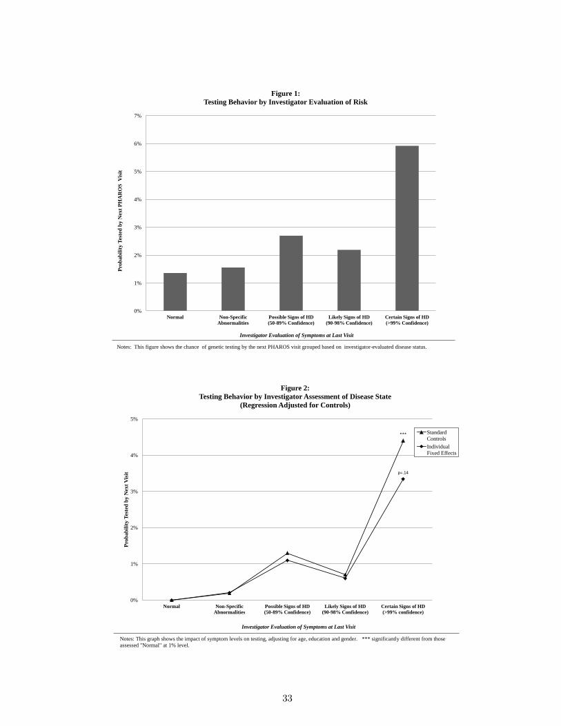
0%
1%
2%
3%
4%
5%
6%
7%
Normal Non-Specific
Abnormalities
Possible Signs of HD
(50-89% Confidence)
Likely Signs of HD
(90-98% Confidence)
Certain Signs of HD
(>99% Confidence)
Pro
ba
bil
ity
Tes
ted
by
Nex
t P
HA
RO
S V
isit
Investigator Evaluation of Symptoms at Last Visit
Figure 1:
Testing Behavior by Investigator Evaluation of Risk
Notes: This figure shows the chance of genetic testing by the next PHAROS visit grouped based on investigator-evaluated disease status.
***
p=.14
0%
1%
2%
3%
4%
5%
Normal Non-Specific
Abnormalities
Possible Signs of HD
(50-89% Confidence)
Likely Signs of HD
(90-98% Confidence)
Certain Signs of HD
(>99% confidence)
Pro
ba
bil
ity
Tes
ted
by
Nex
t V
isit
Investigator Evaluation of Symptoms at Last Visit
Figure 2:
Testing Behavior by Investigator Assessment of Disease State
(Regression Adjusted for Controls)
Standard
Controls
Individual
Fixed Effects
Notes: This graph shows the impact of symptom levels on testing, adjusting for age, education and gender. *** significantly different from those
assessed "Normal" at 1% level.
33

0
0.01
0.02
0.03
0.04
0.05
0.06
0.07
0.08
0.09
-3 -2 -1 0 1 2 3 4
Ch
an
ce T
este
d B
etw
een
Per
iod
t-1
an
d t
Change in UHDRQ Period t-2 to t-1
Figure 3:
Testing Behavior by Change in Investigator Score
All
Baseline
UHDRQ = 0
Notes: This graph shows the relationship between changes in investigator confidence about disease status and subsequent testing. Investigator confidence is on a range from 0 to 4
with 0 indicating no evidence of HD and 4 indicating HD with >99% confidence. The X-axis shows changes between visits t-2 and t-1 and the Y-axis shows the chance tested
between visits t-1 and t.
0%
1%
2%
3%
4%
5%
26-30 31-35 36-40 41-45 46-50 51-55 56-60
Ch
an
ce T
este
d b
y N
ext
Vis
it
Age: Older Individuals Have Lower HD Risk
Figure 4:
Testing Behavior by Age among Individuals with No Symptoms
Notes: This graph shows testing rates by age among individuals with no symptoms. As individuals age their risk falls, from around 50% for the
youngest group to 5-10% for the oldest.
34

0%
10%
20%
30%
40%
50%
60%
70%
80%
90%
100%
1 2 3 4 5 6 7 8 9 10 11-15 16-20 21-30 >30
Per
ceiv
ed R
isk
, Act
ua
l R
isk
or
Sh
are
Rep
ort
ing
No
Ris
k
Motor Score
Figure 5:
Perceived and Actual Risk of HD, by Motor Score
Chance of HD
based on Motor
Signs
Reported
Chance of HD
Share Reporting
No Chance of
HD
Notes: This figure shows the reported chance of HD (individual perception) and the actual posterior chance of HD by motor score.
**,++
**,++
***,+++
***, +++
***,+++
-0.05
0.00
0.05
0.10
0.15
0.20
0.25
Pregnancy Marriage Retire Major Financial Change Change in Recreation
Ch
an
ce o
f B
eha
vio
r, R
ela
tiv
e to
Tes
ted
wit
ho
ut
Mu
tati
on
Figure 6:
Behavior Choice Relative to Individuals Without HD Expnansion
Untested
Certain Have HD
Expansion
Notes: The bars shows differences in behavior relative to individuals who report they do not carry the HD expansion. Untested individuals include
only individuals who report being uncertan about their stauts. Those who carry the mutation know that they carry it either through testing or through
early symptoms. The regression adjusts for age ,gender and education. The regression for pregnancy restricts to people under 40 and also adjusts for
number of existing children. ** ,***significantly different from those without mutation at 5% and 1% levels. ++,+++ significantly different from
untested group at 5% and 1% levels.
35

Figure 7: Optimal Expectation Model, Graphical Intuition
-1
-0.5
0
0.5
1
1.5
2
0 0.1 0.2 0.3 0.4 0.5 0.6 0.7 0.8 0.9 1
Uti
lity
(δ=.
8,Φ
=Ω=.
9)
p
Figure 7.1: Optimal Expectations Model, Time 1 Ancitipatory Utility
Time 1 Utility with Testing
Time 1 Utility Without Testing
Difference (Testing -No Testing)
p*=.92
0
0.2
0.4
0.6
0.8
1
1.2
1.4
1.6
1.8
2
0 0.1 0.2 0.3 0.4 0.5 0.6 0.7 0.8 0.9 1
Uti
lity
(δ=.
8,Φ
=Ω=.
9)
p
Figure 7.2: Optimal Expectations Model, Time 2 Consumption Utility
Time 2 Utility with Testing
Time 2 Utility Without Testing
Difference (Testing -No Testing)
p*=.92
p*=.92
-0.2
0
0.2
0.4
0.6
0.8
1
0 0.1 0.2 0.3 0.4 0.5 0.6 0.7 0.8 0.9 1
Uti
lity
(δ=.
8,Φ
=Ω=.
9)
p
Figure 7.3: Optimal Expectations Model, Total Value of Testing
Total Value of Testing
ψ (for reference)
p*=.92

Table 1: Summary Statistics
Panel A: HD Status VariablesMean Std. Dev. # of Obs.
Motor Score (0-100) 4.00 6.66 3267Doctor Evaluation of Risk (0-4 Scale) 0.634 0.999 6501Perceived Chance of HD Mutation (untested) 42.9% 24.7% 2768Tested (0/1) 4.6% 20.9% 6779Tested Positive (0/1) (if test status inferred) 57.4% 49.5% 287
Panel B: Life Experience Summary StatisticsMean Std. Dev. # of Obs.
Pregnant (Self or Partner), Under 40 11.4% 31.8% 865Get Married (if unmarried) 14.5% 35.3% 884Get Divorced 2.7% 16.1% 3633New Job 14.6% 35.3% 3050Retire 1.2% 10.7% 3057Major Financial Change 38.9% 48.7% 3218Change in Church Attendance 8.5% 27.9% 3161Change in Recreation Activities 19.4% 39.5% 3159
Panel C: Demographic Summary StatisticsMean Std. Dev. # of Obs.
Age 41.8 7.3 1001Male (0/1) 29.3% 45.5% 1001Education (years) 14.9 2.6 1001
Notes: This table shows simple summary statistics from the PHAROS data. In Panels A and B an observation isan individual-year, since perceived probability and doctor score can both vary across visits for a given individualand actions are chosen in multiple years. In Panel C there is just one observation per individual. Oster et al(2010) detail the methodology for inferring test results for tested individuals.
36

Table 2: Behavior Among Individuals with Certain HD Status
Difference in Mean Probability Coefficient Adjusted for ControlsWith HD Mutation - With HD MutationWithout HD Mutation Relative to Without Mutation
(1) (2)Pregnant (Self or Partner), Under 40 0.141∗∗ 0.223∗
Get Married (if Unmarried) 0.140∗ 0.168∗∗
Get Divorced 0.019 0.013New Job 0.003 -0.0164Retire 0.034∗ 0.031Major Financial Change 0.162∗∗∗ 0.132∗∗
Change in Church Attendance 0.015 0.0172Change in Recreation Activities 0.167∗∗∗ 0.123∗∗∗
Notes: This table shows, for each action, the relative probability of taking the action in the last year for individuals
who are certain they do or do not carry the HD mutation. Column 1 shows the basic difference in means (significance
from t-tests); Column 2 shows the coefficients from a regression adjusting for simple controls (gender, education, age and
previous children in the case of pregnancy). ∗significant at 10% ∗∗significant at 5% ∗∗∗significant at 1%.
37

Table 3: Behavior by HD Symptom Levels
(1) (2) (3) (4) (5) (6)
Dependent Variable: Pregnancy Get Married Retire Major Change All Behaviors
(Self or Partner) Finance Change in Recreation
Sample: Age<40 Unmarried All All All All
Uncertain, Motor=0 .0455 .0251 -.0083 .0020 -.0374 -.0055
(.052) (.047) (.008) (.032) (.026) (.014)
Uncertain, Motor 1-3 -.0073 .0227 -.0128 -.0043 -.0392 -.0055
(.054) (.049) (.008) (.034) (.028) (014)
Uncertain, Motor 4-6 .064 .0390 -.0207∗∗ -.0152 .0108 .0001
(.062) (.054) (.009) (.039) (.031) (.017)
Uncertain, Motor 7-10 .0319 -.0214 -.0211∗∗ -.0302 .0249 -.0042
(.077) (.057) (.010) (.043) (.035) (.019)
Uncertain, Motor >11 .1176 -.0035 .0108 .0093 .0563 .0226
(.08) (.055) (.010) (.043) (.035) (.022)
Certain Carry Mutation .2148∗∗ .1212∗∗ .0353∗∗∗ .1446∗∗∗ .1442∗∗∗ .1100∗∗∗
(.090) (.062) (.012) (.050) (.040) (.024)
General Controls YES YES YES YES YES YES
# Children YES NO NO NO NO NO
# of Observations 505 593 2878 3029 2977 9251
Notes: This table reports estimates of differences in behavior for individuals with varying risk of HD. The omitted
category is individuals who are certain they do not carry the mutation. Uncertain individuals are those who report an
intermediate probability of carrying the mutation; we differentiate them by their doctor-assigned motor score, which
ranges from 0 (no symptoms) up to 100 (which would indicate extremely advanced HD). The true updated probability of
HD for each motor score group can be seen in Figure 6. The certain group contains those individuals who report being
sure they carry the HD mutation. General controls are: fixed effects for ten year age group, gender, years of education.
When we estimate impacts on pregnancy we also control for the number of existing children. The final column estimates
the impact on all behaviors together, with the data stacked so the observation is an individual-behavior. In this case
we control for dummies for each behavior and cluster the standard errors by individual. Standard errors in parentheses.∗significant at 10% ∗∗significant at 5% ∗∗∗significant at 1%.
38

Table 4: Estimated Parameter Values and Moments
Panel A: Estimated Parameter ValuesOptimal Expectations Neoclassical ModelMean 95% CI Mean 95% CI
α .856 (.855,.857) 10.006 (7.41,568.4)α+ β .958 (.956,.959) 10.008 (7.41,568.4)δ .968 (.967,.969)λ .00009 (2.30e-5,.0006)λ+ β .0017 (.00056,.0036)
Panel B: MomentsMoments in Data Optimal Expectations Neoclassical Model
Motor Score Group Behavior Testing Behavior Testing Behavior Testing0 (p = .4) 0.00 1.49% 0.000 2.05% 0.000 3.71%1-3 (p = .54) 0.00 0.86% 0.000 2.72% 0.000 5.03%4-6 (p = .6) 0.0006 2.3% 0.000 3.25% 0.000 5.74%7-10 (p = .75) 0.00 4.0% 0.000 4.23% 0.000 6.99%>11 (p = .98) 0.204 4.6% 0.210 2.99% 0.225 8.04%
Notes: This table shows estimated parameter values (Panel A) and moments (both behavior and testing) fromthe data and the estimated model (Panel B). Estimation is done using method of simulated moments in Matlab.In the optimal expectations model, Φi˜Unif[α, α + β]. In the neoclassical model, Φi ∼ Unif[α, α+β] andΩi ∼ Unif[λ, λ+ β].
Table 5: Counterfactuals
Change in Model Simulated Testing Rate(1) No Change 2.39%(2) Zero Cost of Testing 9.05%(3) Double Testing Cost 1.14%(4) δ = 1 0%(5) δ = .9 54.7%(6) α = .8 0%(7) α = .9 30.8%
Notes: This table shows the simulated testing rate (average across all individuals) for the parameter values inTable 4 (row 1) and variations (rows 2-7). The baseline cost of testing is C = .01.
39

Appendix A: Life Events Questionnaire INSTRUCTIONS: Listed below are a number of events, which can bring about change in the lives of those who experience them. Please mark "YES" for the events that you have experienced in the last year. Also, for each item marked "Yes" below, indicate the extent to which you viewed the event as having either a positive or negative impact on your life at the time the event occurred.
Yes
N
o Ex
trem
ely
Neg
ativ
e M
oder
atel
y N
egat
ive
Slig
htly
Neg
ativ
e N
o Im
pact
Sl
ight
ly P
ositi
ve
Mod
erat
ely
Posi
tive
Extre
mel
y Po
sitiv
e
1. Marriage 2. Detention in jail or comparable institution 3. Death of spouse 4. Major change in sleeping habits (If No go to #5)
4a. If Yes, in question 4, trouble falling asleep 4b. If Yes, in question 4, trouble staying asleep 4c. If Yes, in question 4, early morning wakening
5. Death of close family member: If Yes, complete remainder of question. Mother Affected by HD? Father Affected by HD? Brother Affected by HD? Sister Affected by HD? Grandmother Affected by HD? Grandfather Affected by HD? Other (specify): Affected by HD?
6. Major change in eating habits (If No go to #7) 6a. If Yes, in question 6, have you lost more than
10% of your previous body weight? 6b. If Yes, in question 6, have you gained more
than 10% of your previous body weight? 7. Foreclosure on mortgage or loan

Yes
N
o Ex
trem
ely
Neg
ativ
e M
oder
atel
y N
egat
ive
Slig
htly
Neg
ativ
e N
o Im
pact
Sl
ight
ly P
ositi
ve
Mod
erat
ely
Posi
tive
Extre
mel
y Po
sitiv
e
8. Death of a close friend 9. Outstanding personal achievement 10. Minor law violations (i.e. traffic ticket) 11. Wife / girlfriend's pregnancy 12. Your own pregnancy 13. Change in work situations (responsibilities, hours, etc.) 14. New job 15. Serious illness or injury of close family member:
15a. Mother 15b. Father 15c. Brother 15d. Sister 15e. Grandmother 15f. Grandfather 15g. Other (specify):
16. Sexual difficulties 17. Trouble with employer (i.e. danger of losing job) 18. Trouble with in-laws 19. Major change in financial status 20. Major changes in closeness of family members 21. Gaining a new family member (i.e. birth,
adoption, family member moving in) 22. Change of residence 23. Marital separation from spouse, due to conflict 24. Major change in church activities 25. Marital reconciliation with mate 26. Major change in number of arguments with spouse 27. Change in wife's work outside the home 28. Change in husband's work 29. Major change in usual type and/or amount of recreation 30. Borrowing more than $10,000

Yes
N
o Ex
trem
ely
Neg
ativ
e M
oder
atel
y N
egat
ive
Slig
htly
Neg
ativ
e N
o Im
pact
Sl
ight
ly P
ositi
ve
Mod
erat
ely
Posi
tive
Extre
mel
y Po
sitiv
e
31. Borrowing less than $10,000 32. Being fired from job 33. Wife / girlfriend having an abortion 34. Having an abortion 35. Major personal illness or injury 36. Major change in social activities (i.e. parties, movies,
visiting - increased or decreased participation) 37. Major changes in living conditions of family (i.e.
building new home, remodeling) 38. Divorce 39. Serious injury or illness of close friend 40. Retirement from work 41. Son or daughter leaving home 42. Ending of formal schooling 43. Separation from spouse, due to work, travel, etc. 44. Engagement 45. Breaking up with boyfriend / girlfriend 46. Leaving home for the first time 47. Reconciliation with boyfriend / girlfriend 48. Taking on major care - taking responsibilities for a
family member (If No go to question 49) 48a. If Yes, in question 48, who? 48b. If Yes, in question 48, is this person affected
with HD? Other experiences having an impact on your life: (please list and rate) 49. 50. 51. 52. Have you made a living will? 53. Have you made arrangements for durable (enduring)
power of attorney?
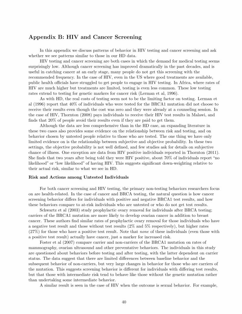
Appendix B: HIV and Cancer Screening
In this appendix we discuss patterns of behavior in HIV testing and cancer screening and askwhether we see patterns similar to those in our HD data.
HIV testing and cancer screening are both cases in which the demand for medical testing seemssurprisingly low. Although cancer screening has improved dramatically in the past decades, and isuseful in catching cancer at an early stage, many people do not get this screening with therecommended frequency. In the case of HIV, even in the US where good treatments are available,public health officials have struggled to get people to engage in HIV testing. In Africa, where rates ofHIV are much higher but treatments are limited, testing is even less common. These low testingrates extend to testing for genetic markers for cancer risk (Lerman et al, 1996).
As with HD, the real costs of testing seem not to be the limiting factor on testing. Lerman etal (1996) report that 40% of individuals who were tested for the BRCA1 mutation did not choose toreceive their results even though the cost was zero and they were already at a counseling session. Inthe case of HIV, Thornton (2008) pays individuals to receive their HIV test results in Malawi, andfinds that 20% of people avoid their results even if they are paid to get them.
Although the data are less comprehensive than in the HD case, an expanding literature inthese two cases also provides some evidence on the relationship between risk and testing, and onbehavior chosen by untested people relative to those who are tested. The one thing we have onlylimited evidence on is the relationship between subjective and objective probability. In these twosettings, the objective probability is not well defined, and few studies ask for details on subjectivechance of illness. One exception are data from HIV positive individuals reported in Thornton (2011).She finds that two years after being told they were HIV positive, about 70% of individuals report “nolikelihood” or “low likelihood” of having HIV. This suggests significant down-weighting relative totheir actual risk, similar to what we see in HD.
Risk and Actions among Untested Individuals
For both cancer screening and HIV testing, the primary non-testing behaviors researchers focuson are health-related. In the case of cancer and BRCA testing, the natural question is how cancerscreening behavior differs for individuals with positive and negative BRCA1 test results, and howthese behaviors compare to at-risk individuals who are untested or who do not get test results.
Schwartz et al (2003) study prophylactic ovary removal for individuals after BRCA testing;carriers of the BRCA1 mutation are more likely to develop ovarian cancer in addition to breastcancer. These authors find similar rates of prophylactic ovary removal for those individuals who havea negative test result and those without test results (2% and 5% respectively), but higher rates(27%) for those who have a positive test result. Note that none of these individuals (even those witha positive test result) actually have cancer, just a marker for increased risk.
Foster et al (2007) compare carrier and non-carriers of the BRCA1 mutation on rates ofmammography, ovarian ultrasound and other preventative behaviors. The individuals in this studyare questioned about behaviors before testing and after testing, with the latter dependent on carrierstatus. The data suggest that there are limited differences between baseline behavior and thesubsequent behavior of non-carriers, but very large changes in behavior for those who are carriers ofthe mutation. This suggests screening behavior is different for individuals with differing test results,but that those with intermediate risk tend to behave like those without the genetic mutation ratherthan undertaking some intermediate behavior.
A similar result is seen in the case of HIV when the outcome is sexual behavior. For example,
40

Thornton (2008) uses a randomized evaluation in Malawi to estimate the impact of learning HIVstatus on risky behavior and condom purchases. She finds evidence that those who learn about apositive test result purchase more condoms, but there is no difference between those who learn abouta negative result and those who remain uninformed. She also finds a large (but not significant)decrease in risky sexual behavior for individuals who test positive. A meta-analysis of data from theUS from 1985 to 1997 (Weinhardt et al, 1999) shows similar patterns. Risky behavior (lack ofcondom use, unprotected sex) is similar for untested individuals and those with a negative testresult; those with a positive test result have significantly less risky behavior.
Overall, in both cases, the data suggest that behaviors are very different for individuals withdiffering test results, as we would expect. We also consistently observe that individuals withintermediate risk do not undertake some intermediate level of behavior: they appear to behave muchmore similar to individuals who have a negative test result. This suggests some “skewing” of actionstoward what would be optimal in the good state.
Risk and Testing Behavior
Among the most informative genetic screens for cancer is the test for the BRCA1 or BRCA2mutation, which are a strong predictors of both breast and ovarian cancer. Penentrance of thesemarkers is high: 80% of women with the BRCA1 mutation will develop breast cancer if they live toage 80. A simple way to measure ex ante risk is with the number of relatives impacted by breastcancer: the more relatives with cancer, the more likely that it is genetic. In a number of studies oftesting behavior, it appears that testing is increasing with risk, as measured by number of familymembers impacted (Lerman et al, 1996; Meijers-Heijboer et al, 2000; Baer et al, 2010). The secondof these studies (Meijers-Heijboer et al, 2000) explicitly separates individuals at 25% risk from thoseat 50% risk and shows higher testing rates among the 50% risk group.
Cancer screening (mammography in particular) shows similar patterns. In a meta-analysisfocusing on perceived risk and screening behavior, Katapodi et al (2004) demonstrates that perceivedrisk is associated with increased screening behavior.
In the case of HIV testing in the US, testing also seems to be increasing in risk (Wortley et al,1995; Stein and Nyamathi, 2000; Samet et al, 1997). The African context is perhaps moreinteresting, given extremely low testing rates and high prevalence in many countries in the region,and shows more mixed evidence. A number of studies find self-perceived risk increases testing(Wringe et al, 2008; Adeneye et al, 2006; Fylkesnes and Siziya, 2004), although some have found theopposite (Sambisa et al, 2010; Thierman et al, 2006).
It is worth noting that this evidence is weaker than the HD evidence in the sense that to alarge extent these behaviors are directly linked to disease risk, disease avoidance or diseasetransmission and, given that, it seems inherently more likely that those with positive test resultswould respond more. This underscores the advantage of the HD setting and data.
Appendix C: Alternative Non-Neoclassical Models
In this section we describe two alternative, non-neoclassical, models which have been suggestedto explain these behaviors.
41

Wishful Thinking (Mayraz, 2011)15
The key assumptoin of this model is that individuals engage in “wishful thinking”: when facedwith a bad state of the world, they are overly optimistic. More concretely, individuals hold subjectivebeliefs which depend on the payoff function. We describe the setup and results below.
Setup
As before, there is a binary state s ∈ 0, 1 and individuals are endowed with p = E(s). Thestarting point in this model is bias in subjective beliefs: the assumption that individuals engage inwishful thinking causes their beliefs to be (potentially) biased toward the healthy state. As in thebasic setup, we assume that individuals prefer to be healthy than to be sick. We denote the utilityfrom health as f(s). As in the body of the paper, we assume that f(s = 1) = 0 and f(s = 0) = 1,implying that the maximum possible utility in the healthy state is 1 and in the sick state is 0.
In general, Mayraz (2011) describes the formulation of subjective beliefs π(s) from objectiveprobabilities p(s) as: π(s) = p(s)eψf(s) where ψ represents the level of optimism. Someone with avalue of ψ = 0 is a realist; high values of ψ indicate high optimism. This model can alsoaccommodate pessimism (with a negative ψ). In the HD case, the subjective probability can becomputed
π =peψ(f(s=1))
peψ(f(s=1)) + (1− p)eψf(s=0)=
p
p+ (1− p)eψ
As in the baseline model, individuals choose a binary action a ∈ 0, 1. Utility in this model isdelivered in the same way as in the optimal expectations model:
U((a, s)|p) = δE(u(a, s)|π) + E(u(a, s)|p)
where a = argmaxaE[u(a, s)|π]. However, in this model individuals consider only the anticipatoryutility period when making choices about testing. In the optimal expectations model individualsmake a choice of action based only on the beliefs in the anticipation period, but make choices abouttesting based on both periods. In this case, both action and testing choices are made based only onthe anticipatory period, so we can write the object that individuals actually maximize asU((a, s)|p) = E[u(a, s)|π]. For simplicity, we assume symmetric values for utility losses, so we have:
u(0, 1) = −Φu(1, 1) = 0u(1, 0) = 1− Φu(0, 0) = 1
We assume that testing carries a real financial cost C.
Results
Results on beliefs and actions are shown in Appendix Proposition 3.
Appendix Proposition 1. Beliefs and Actions15We are extremely grateful to Guy Mayraz for very helpful conversation about this model, and for developing the
version of the model we present here.
42

1. If ψ > 0 individuals hold beliefs π < p.
2. Action a = 0 will be taken for values of p∗ ≤ eψ
1+eψ
Proof. 1. As noted above, in this model π = pp+(1−p)eψ . As long as ψ > 0 this is less than p.
2. Lemma 1 in the paper describes the choice of action based on π. The model here corresponds
to the symmetric case, so the cutoff value to switch from a = 0 to a = 1 is π = .5. This
statement follows directly from solving for p when π = .5
The intuition for this result is similar to the optimal expectations case, although the result isdelivered with one fewer step. By assuming biased beliefs, we deliver that result immediately, andthe actions follow.
We next turn to testing behavior. The proposition below describes the relationship betweentesting and risk, the condition for individuals to test at all, and the condition for confirmatorytesting. As in the optimal expectations case, we assume that testing for confirmation carries a valueΨ.
Appendix Proposition 2. Testing Behavior
1. Value of testing is increasing in p for values of p < p∗ where p∗ = eψ
1+eψ. Value of testing is
decreasing in p for values of p ≥ p∗.
2. Individuals will test if either:
(a) p < p∗ and π(p)Φ > C or
(b) p ≥ p∗ and (1− π(p))Φ > C
3. Confirmatory testing will occur without predictive testing if and only if Ψ > Φ.
Proof. 1. Both points (1) and (2) follow from the value of testing. If π(p) ≤ .5 and individuals aretaking action a = 0 then value of testing is Vtest = π(p)Φ. If π(p) > .5 and individuals aretherefore taking action a = 1 then Vtest = (1− π(p))Φ. Note that p∗ is the value such thatπ(p∗) = .5. Testing value is therefore increasing up to this p∗and decreasing for higher values.Moreover, in either case individuals will test if the value to testing exceeds the real cost.
2. To have confirmatory testing without predictive testing requires that individuals want to testfor confirmation but not for predictive reasons. Testing for confirmation requires that Ψ > C.Not testing predicatively requires that the value to testing for confirmation only be higher than
43

the value to testing predictively, where the latter is evaluated at the highest testing value point(p∗, or π = .5), at which point individuals are still taking action a = 0. These values are given:
Vtest,predictive = .5u(1, 1) + .5u(0, 0)− C + πΨVtest,confirmation = .5u(0, 1) + .5u(0, 0) + .5(Ψ− C)
Testing for confirmation and not predictively will therefore occur if C > Φ. Together with thecondition for testing for confirmation rather than not testing at all, we have Ψ > Φ.
This model delivers the implication that testing is increasing in p directly through the wishfulthinking. As an a neoclassical model, individuals want to test when they are most uncertain (whenthey believe the probability of the disease is 50%). Because of the wishful thinking, this occurs at anobjective probability of higher than 50%, namely at p∗.
The other parts of Appendix Proposition 4 are more similar to the rational model. Individualsare prevented from testing here only by the real cost of testing, and therefore this cost must be highin order to prevent testing. In particular, for the same parameter values preventing testing requires ahigher cost of testing than in the optimal expectations model. The required cost is not as large as inthe neoclassical model, however, since there the value of testing was pΦ, and here it is πΦ and, asshown in Appendix Proposition 3, π < p.
With regards to confirmatory testing, this model has an issue similar to the rational model.Generating confirmatory testing requires that the gain to confirmatory testing be larger than thegain to taking the correct actions up to that point. We have argued this is not the case, so effectivelythis model cannot rationalize confirmatory testing behavior.
Summary
In many ways this model is observationally similar to the optimal expectation case, given whatwe can see in our data. Both models predict biased beliefs, skewed actions and testing increasing inrisk. In terms of the predictions on beliefs, this model may actually be a better fit than the optimalexpectations, since it accommodates the fact that reported beliefs are increasing in actual risk, evenif slowly, rather than suggesting all biased beliefs are π = 0.
The two models have different psychological micro-foundations, but testing between these isbeyond the scope of our data. More specifically, the underpinnings of the optimal expectations modelsuggest that individuals “know” their true p – it’s effectively a two-self model in which, if pushed,individuals could in principle access their true risk, even if they are adopting biased beliefs. Thewishful thinking model has only the biased beliefs. Through wishful thinking individuals literallyforget their true risk. Although this does differentiate the models, it’s not something we can test inour data.
The most significant difference between this and the optimal expectations model comes in thetesting. Like the neoclassical model, there is nothing limiting testing here other than real testingcosts. This means that both (a) higher real testing costs would be required to rationalize low testingrates and (b) this model struggles to explain confirmatory testing. For this reason, we favor theoptimal expectations setting, although the similarities between the models make this a plausible
44

alternative. Richer data, with more information on psychological processing of these decisions, mighthelp differentiate the two.
Information-Averse Preferences
Setup
We retain the basic setup from Section 4.1. The state is binary (s ∈ 0, 1) and individualshave some exogenously given p = E(s). Consumption utility at time 2 is given by:U2 = E[u(a, s)|p] = pu(a, 1) + (1− p)u(a, 0).
Individuals also experience some anticipatory utility at time 1. Individuals haveinformation-averse preferences over anticipatory utility (Kreps and Porteus, 1978). We adopt anextremely simple formation for time 1 utility (or “anxiety”), drawn from Caplin and Leahy (2004):U1 = c(1− p)− b
(p− 1
2
)2, with c, b > 0. The c(1− p) term indicates an individual with these
preferences would prefer a low p, since it indicates they are unlikely to be sick. However, thisindividual also (all else equal) has a preference for uncertainty: as p moves away from 1
2 in eitherdirection, utility falls. We can interpret c as a general disutility of being sick. We interpret b as thedegree to which the individual dislikes uncertainty.16
Since action choices do not enter time 1 utility, a∗ is determined based only on consumptionutility at time 2, so a∗(p) = argmaxa[pu(a, 1) + (1− p)u(a, 0)]. Total two period utility is given bythe equation below.
U(a, s, p) = c(1− p)− b(p− 1
2
)2
+ pu(a∗(p), 1) + (1− p)u(a∗(p), 0)
We define the parameter values as in Section 4.
u(0, 1) = −Ωu(1, 1) = 0u(1, 0) = 1− Φu(0, 0) = 1
Results
We summarize the results in two propositions. The first describes beliefs and actions. Thesecond describes the relationship between testing and risk. We discuss confirmatory testing at theend.
Appendix Proposition 3. Beliefs and Actions
1. Self-reported beliefs are accurate (π = p)
2. Action a = 0 is taken as long as p < p∗ where p∗ = ΦΦ+Ω . Note p∗ > .5 iff Φ > Ω.
16In principle, this taste for uncertainty could imply people actually prefer p = .5 to p = 0, which seems unlikely;however, with high enough c this will not be the case.
45

Proof. 1. This follows directly from the fact that the model does not accommodate the possibility
of beliefs other than p.
2. Note that the action utility enters only at time 2. The individual will choose a = 0 if
(1− p)Φ ≥ pΩ. Rearranging, we find that the individual will choose a = 0 up to a value of
p∗ = ΦΦ+Ω. . Note this is the same as the neoclassical case.
This proposition notes first that this model cannot accommodate biased beliefs. Second, itdemonstrates that generating skewed actions in this model requires the same type of asymmetry asin the neoclassical case, summarized in Section 5 in the paper.
Appendix Proposition 4. Testing and Risk Define p∗ = ΦΦ+Ω , as above. Individuals will choose
to test if one of the following conditions holds:
1. p ≤ p∗ and p > b−Ωb
2. p > p∗ and p < Φb
Proof. 1. When p ≤ p∗ the individual is taking action a = 0. Given this, Vtest = pΩ + b(p2 − p).This is positive for values of p > b−Ω
b .
2. When p > p∗ the individual is taking action a = 1. Given this, Vtest = (1− p)(Φ− bp). This ispositive when Φ− bp > 0
For values of p below p∗, the utility from testing has two components. First, over this range ofp, individuals take the action a = 0. As p increases, it becomes more and more likely this is wrongand the value to learning the true state and taking the correct action increases. This component ofthe testing utility is always positive. Pushing against this is the anxiety associated with testingwhich is the difference in anticipation utility if tested versus untested: − b
4 + b(p− 1
2
)2. This
difference is the greatest (most negative) when p = .5. If b is large enough, this anxiety may be largeenough to outweigh the positive benefits of testing and individuals may prefer not to test.
For small values of b, individuals with p < p∗ will always want to test. The model requires
values of b > Ωin order to generate any testing avoidance over this range. Given that b > Ω, testing
value will be increasing with p up to p∗, which could produce the result that testing is increasing in
risk; to have testing value be highest somewhere above 0.5 it must be the case that b > 2Ω.
For value of p > p∗, the value of testing is decreasing in p. If Φ > b then the actor will want to
test for any value of p > p∗. If b > Φ they may test only for values of p closer to p∗.
46

It is worth noting that, while this model does include the assumption that people prefer tohave a lower p (in the form of the c(1− p) term), this does not enter the decision-making abouttesting. Because this is linear in p, from the standpoint of someone deciding whether or not to test,individuals experience the same value for this (in expectation) whether or not they choose testing.
Confirmatory testing fits easily in this model. Individuals avoid testing here not due to testingcosts but due to preferences for information avoidance. Once those concerns are removed (as theywould be once the individual was sure of their status) they would be willing to test if Ψ(the value ofconfirmation) is greater than the cost of testing. This relationship has no bearing on the desire toavoid testing in the anticipation period.
Summary
Under some conditions, this model can fit the data. However, it shares two problems with theneoclassical model. First, it does not allow for overly-optimistic beliefs. To the extent this is a factwe would like to fit, the model fails there. In addition, explaining the skewed actions and testingincreasing in risk requires some asymmetry in the loss to the wrong action in the two states (just asin the neoclassical model). As we discuss in Section 5, there is not a lot of empirical support for thatclaim. The latter result on testing and risk also requires a particular set of parameter values for brelative to Ω, an assumption which is plausible but difficult to test. Where this model clearlypreforms better than the neoclassical model is on the testing costs and testing confirmation: it isable to explain limited testing without resorting to the extremely high testing costs and it canaccommodate the confirmatory testing easily.
47


