OPEN ECONOMY MACROECONOMICS
Prof. Alemayehu GedaGuest Lecture (UoN)
School of EconomicsUniversity of Nairobi
(Adopted from Mr. Rup Singh)Lecture 1

Objectives:
1. Extend the closed economy IS-LM model to include the external sector.
2. Evaluate the relevance of fiscal and monetary policies at the disposal of policy makers.
3. Analyze how the domestic economy performs, given the international macroeconomic conditions.
4. Carry out quantitative analysis of various polices/shocks to the economy vis-a-vis the extended IS-LM model.

The international conditions sometimes give us (domestic economy) opportunities and sometimes, pose threats to us also.
Therefore, the more an economy is integrated into the global village (through globalisation), the more severe these impacts will be. [Being totally closed is not a viable option for various reasons]
Growing international interdependence implies booms and recessions in one country spills over to other country. [When America sneezes, the world catches cold!]
Economies are linked through trade flows and changes in interest (exchange) rate. [The first affects trade accounts and external debt and the second affects capital account flows.]
For example, the Asian Crisis of 1997-99 was limited to few countries initially but spread to other countries, affecting global economic growth. Same with the 2008 Global Crisis in the West We call this
“The Contagion effect”
In this lecture, basic facts (empirical evidence) and models of international economic linkages are introduced and discussed.

We will look at the implications of different international macroeconomic conditions on our economic fundamentals.
You should read the text: Donbusch et al. (chap. 11-12) and also read the revised edition (by the same authors) See also my (Alemayehu, 2002) Chapter 6 and Paper on the Impact of the Global Economy on Africa.
You should analyse various discussions/arguments presented on these chapters, as my presentation will be largely based on them.

Coming back to business:
When we think of open economy the first set of questions we ask: How a country with a fixed exchange rate adjusts to balance of payments problems (e.g., persistent deficit in the trade/overall balance; loss of reserves; rising level of debt; pressure on the exchange rate)?
[Note that all the major countries have switched to the floating exchange rate system after 1973 (when the US de-linked the dollar from gold), but many countries, most of them small open economies, continue to maintain a fixed exchange rate system.]
Solving the balance of payments problems generally means getting out of a deficit situation, in the trade account, the current account, the balance of payments account, or in all three accounts simultaneously.
Balance of payments problems are solved through automatic adjustment mechanisms or through changes in economic policy.
Let us see what policy options are there, available to policy makers

But, first of all let’s discuss what is Exchange Rate - the first link to the ROW. Exchange rate is the price one country’s currency expressed in terms of some other country’s currency.
E.g, if we we relate Ksh to the USD as “how much it takes to get 1 USD, in terms of Ksn,” the exchange rate is:
Ks72.2:$1US
This gives the definition of the nominal exchange rate that we will be using now onwards:
E = Ksh/USD
It tell us that the price of 1USD = Ksh72.2.

Kenya’s, currency is tied down to its trading partners’ currencies (Pound, Euro, Japan, and USA).
Most countries in Africa have exchange rate close to fixed, but operate under the so called a Pegged Exchange Rate system. Kenya’s exchange rate is floating
Now, given the definition of the nominal exchange rate, we can define the real exchange rate.
Like any other variable, Real = Nominal /Prices
Therefore the real Exchange rate is Nominal exchange rate adjusted for relative prices (or inflation differentials).
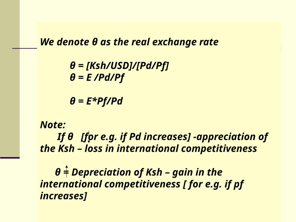
We denote θ as the real exchange rate
θ = [Ksh/USD]/[Pd/Pf]θ = E /Pd/Pf
θ = E*Pf/Pd
Note: If θ [for e.g. if Pd increases] -appreciation of the
Ksh – loss in international competitiveness
θ = Depreciation of Ksh – gain in the international competitiveness [ for e.g. if pf increases]
Then we need to know what is BOP.
BOP is external equilibrium.
It shows whether we have gained or lost from our net exports of goods and services (current account) and whether we are net exporters of importers of investment funds (capital account).
BOP = CA + KA
If we have current account surplus as well as capital account surplus, we will have BOP Surplus.[if CA is in surplus, but KA is in deficit, (or other combinations), BOP depends on the relative magnitudes of surplus or deficit]

Under fixed exchange rate system, a BOP surplus means accumulation of foreign exchange reserves.
On the other hand, a BOP deficit implies a decline in foreign exchange reserves or de-accumulation of forex. reserves.
Note the change in the foreign reserves is the basis for market intervention by the C/Bank under the fixed exchange rate system.
Money supply becomes endogenous in the model. It is no longer under the full control of the C/B.
Capital flow - movement of international speculative investment. One of the determinants of capital flows is the Interest rate.
If interest rate is higher in Kenya, more capital inflow into the economy and v-v – in search for higher RR. Investors look at the differences in returns to investment, which is called the Interest Rate Differentials.
If there are interest differential which favors us (i > if), capital will inflow into Kenya. If interest rate differentials do not favor us, investors will hesitantly invest here, and we say there is imperfect capital mobility.

Other factors that determine capital mobility are:
1. Substitutability of investments2. Tax structure3. Capital controls4. Political/macroeconomic conditions (in search of safe
heavens)(Not also that exchange rate mattera as you may lose what
in exchangre rate what you got as interest rate differential)
In special cases, there are no difference between the interest offered here and that abroad.
In other words, there are no interests rate differentials between the two economies. We call this situation, “perfect capital mobility” - a scenario where our economy is as competitive as any one else’s. (i = if)
So investors are indifferent whether they invest here or anywhere around the globe. Capital flows without hesitation - Perfect Capital Mobility
So given these briefings, we can extend our simple IS-LM model to IS-LM-BP model.
The following slides define the three markets - goods, money and forex markets, from where we derive the IS, LM and the BP equations.
In our analysis of IS-LM-BP Model we will discuss the (Mead) -Mundell-Fleming Model as we proceed.
Mundell and Fleming is an interesting extension to the IS-LM-BP Model, which assumes perfect capital mobility

Open Economy IS-LM-BP Analysis
IS-LM and BP Models

GOODS MARKETC = C0 + cYDYD = Y- T +TR T = T0 + tY I = I0 - bi G = G0, TR = TR0
X= X0 + λθ + γYf
M = M0 + mY – ψθY = C + I + G + NX
FOREIGN EXCHANGE MARKETNX = NX0 – mY + vθ + γYf
CF = CF0 + f(i-if)NX + CF = ΔRES/P
MONEY MARKET
L = kY- hi
Ms/P = M0 /P +ΔRES/P
L = Ms/P
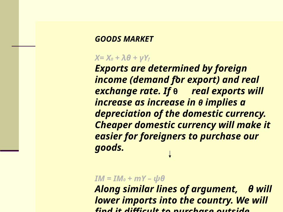
GOODS MARKET
X= X0 + λθ + γYf
Exports are determined by foreign income (demand for export) and real exchange rate. If θ real exports will increase as increase in θ implies a depreciation of the domestic currency. Cheaper domestic currency will make it easier for foreigners to purchase our goods.
IM = IM0 + mY – ψθ
Along similar lines of argument, θ will lower imports into the country. We will find it difficult to purchase outside goods/services once exchange rate appreciates. Imports also depend on domestic income.
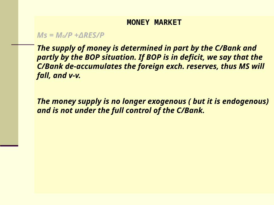
MONEY MARKET
Ms = M0/P +ΔRES/P
The supply of money is determined in part by the C/Bank and partly by the BOP situation. If BOP is in deficit, we say that the C/Bank de-accumulates the foreign exch. reserves, thus MS will fall, and v-v.
The money supply is no longer exogenous ( but it is endogenous) and is not under the full control of the C/Bank.
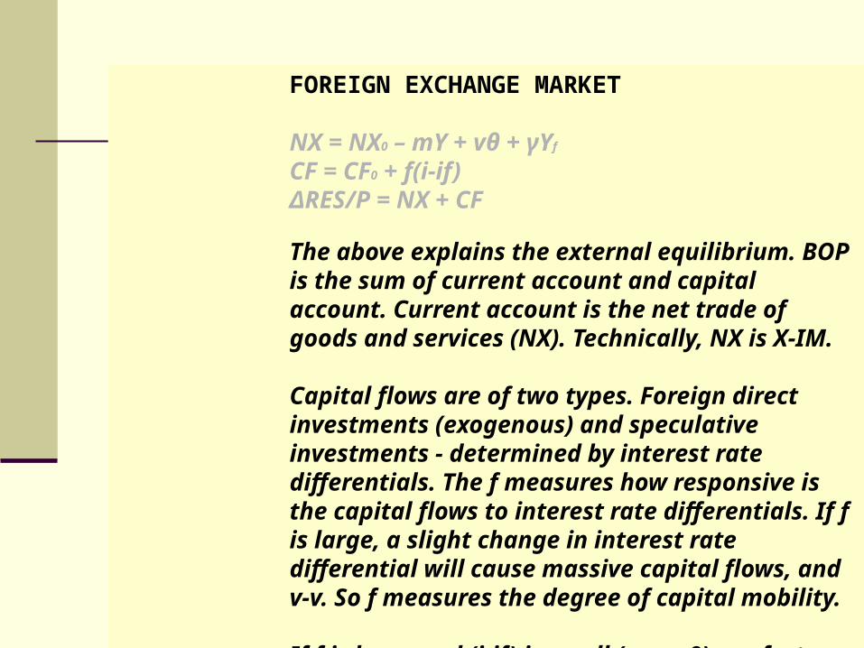
FOREIGN EXCHANGE MARKET
NX = NX0 – mY + vθ + γYf
CF = CF0 + f(i-if)ΔRES/P = NX + CF
The above explains the external equilibrium. BOP is the sum of current account and capital account. Current account is the net trade of goods and services (NX). Technically, NX is X-IM.
Capital flows are of two types. Foreign direct investments (exogenous) and speculative investments - determined by interest rate differentials. The f measures how responsive is the capital flows to interest rate differentials. If f is large, a slight change in interest rate differential will cause massive capital flows, and v-v. So f measures the degree of capital mobility.
If f is large and (i-if) is small (say = 0), perfect capital mobility is implied.If f is very small, no matter how large is (i-if), imperfect capital mobility is implied.

GOODS MARKETC = C0 + cYDYD = Y- T +TR T = T0 + tY I = I0 - bi G = G0, TR = TR0
X= X0 + λθ + γYf
M = M0 + mY – ψθY = C + I + G + NX
FOREIGN EXCHANGE MARKETNX = NX0 – mY + vθ + γYf
CF = CF0 + f(i-if)ΔRES/P = NX + CF
Solving for the Y in each of these markets will give us the IS, LM and BP equations.
MONEY MARKET
Ms/P = M0/P +ΔRES/P
L = kY- hi

Graphical re-presentation of three equations
Y0 Y
IS = -αG/b < 0, negative slopeLM = k/h > 0, positive slopeBP = m/f > 0, positive, but less then k/h. LM is more stepper than BP (u find out why!).
BP (NX0, CF0, θ, if, Yf )
LM (M0, P, ΔRES)
IS (C0, TR0, T0, I0, G0, X0, Imo, θ, Yf )
i
i0

Only under the fixed exchange rate system, there is accumulation or de-accumulation of foreign exchange reserve, which changes Money Supply (Ms), LM curve shifts to restore final equilibrium.
Money supply becomes endogenous – is not under full control of the Central bank. It is made up of domestic base money supply + foreign exchange reserves (BOP surplus) .
Thus C/Bank cannot carry out independent monetary policy under fixed exchange rate.

Numerical Illustration of the MF Model

26
Determinants of Output in an Open Economy
• Aggregate demand depends on consumption, investment, government spending and net exports.
• Consumption depends on disposable income.• Investment on the real interest rate. • Tax revenues on national income.• Exports on foreign income and the real exchange rates. • Imports on domestic income and the real exchange rate.
• The real exchange rate is determined by domestic and foreign price levels and the nominal exchange rates.
• Nominal interest rate is determined in the money market.
• Capital inflow/outflow depends on the difference in the domestic and foreign real interest rates.
• Aggregate supply depends on capital stock and labour force.
27
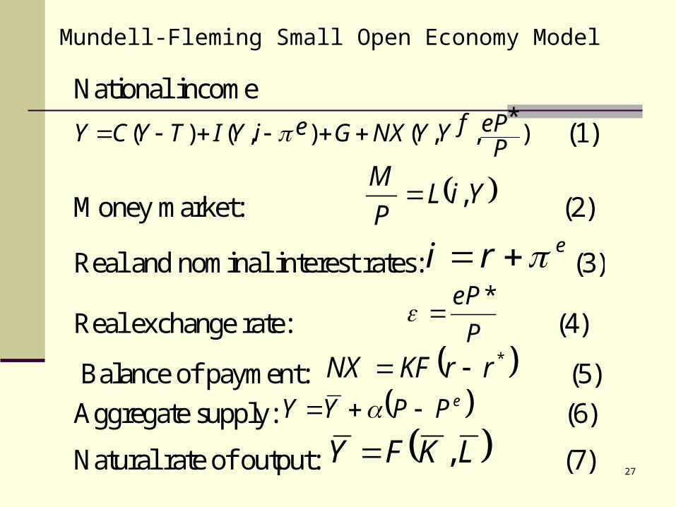
National income
)*
,,(),()(P
ePfYYNXGeiYITYCY (1)
Money market: YiLP
M, (2)
Real and nominal interest rates:eri (3)
Real exchange rate: P
eP * (4)
Balance of payment: *rrKFNX (5)
Aggregate supply: ePPYY (6)
Natural rate of output: LKFY , (7)
Mundell-Fleming Small Open Economy Model

28
Y= Actual output Y =natural rate of output i = nominal interest rate r = real interest rate r* foreign interest rate ε = real exchange rate e = nominal exchange rate. P = price level, P* = foreign price level T = tax rate G =government expenditure M = imports,
K = capital stock, L = labour force, and fY = foreign income
eP = expected domestic price level e = expected inflation.
Endogenous variables (7): Y, Y , i, r, ε, P, e. Exogenous variables (10):
T, G, M, e , P*, r*, eP , K , L and fY
Notations in the Above Open Economy Model

29
TYC 8.0200 iI 20050
201.03.010 YYNX f
P
EP*
%5* ii
T =100 G = 100
,, fYYNXGiITYCY
YiP
M5.050200
National Income
Consumption
Investment
Tax and Spending
Net exports
Real exchange rate
Financial integration
Demand for Money
An Example of an Open Economy Model
500fY 02.0 2* P 2PParameters

30
A Solution of the Model
1280Y 1144C
44I 8NX
S = Y-T-C = 1280 - 100-1144= 36
,, fYYNXGiITYCY =1144 + 44 +100-8=1280
NXISGT 84436100100
Equilibrium Condition:
Model Closure:
Private Saving:

31
Three GAPs: Investment-Saving, Budget and Trade Gaps
i
Saving and Investment
I(r)
S(Y)
TrwLrKXGICMTSCYcall :Re
FlowCapNX
MXGTIS
IS
Private saving +public saving = net export
IS
0NXTrade Surplus
Trade deficit0NX
0
i
0 GTK-outflow
K-inflow
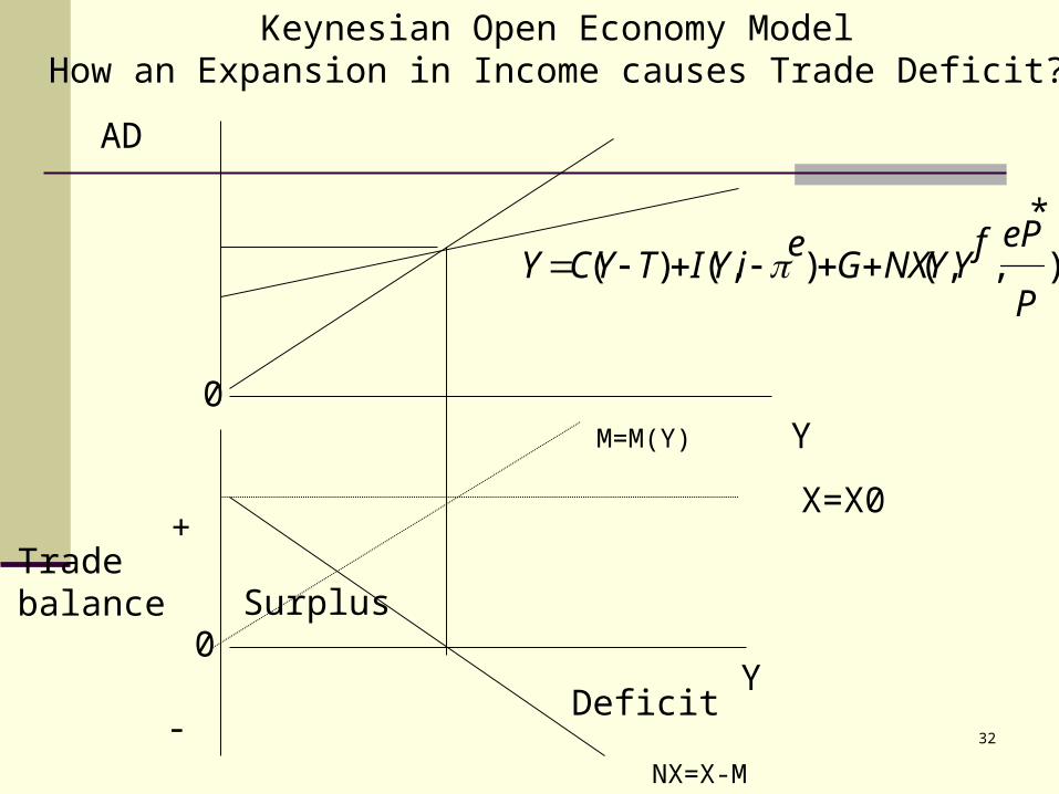
32
0
+
-
Y
Y0
AD
Tradebalance
Keynesian Open Economy ModelHow an Expansion in Income causes Trade Deficit?
)
*
,,(),()(P
ePfYYNXG
eiYITYCY
X=X0
Surplus
Deficit
M=M(Y)
NX=X-M

33
Derivation of Net Exports and Investment Saving in an Open Economy
ΔNX
AD
Y
e2
Y1 Y2
e2
e1 IS*(e)
y1 Y2
AD
NX (e)
NX2 NX1
(a)
(b)(c)
Note:(a) Shows reduction in ADfollowing an increase in ER(b) Shows investment
savingbalance in an open economy(c) Shows net export as a function of the exchange rate(Lower rer=> rise dd for dom
goods=> rise Nx nb rer=e=en*(Pd/pf)
e1

34
IS-LM Model in an Open Economy: Mundell-Fleming Model
IS*
e*
LM (y, i)
Output
Exc
hang
e R
ate
o y
Assumption:Money supply does not depend on exchange rate

35
IS-LM Model in an Open Economy: Mundell-Fleming Model
IS*
e*
LM (y, i)
Output
Exc
hang
e R
ate
o y
Assumption:Money supply does not depend on exchange rate
36
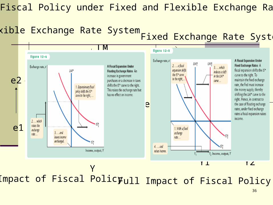
Impact of Fiscal Policy under Fixed and Flexible Exchange Rate Systems
IS*
IS*’
e1
e2
YNo Impact of Fiscal Policy
LM LM1LM2
Fixed Exchange Rate System
Y1 Y2
e
IS*IS*’
Flexible Exchange Rate System
Full Impact of Fiscal Policy
37
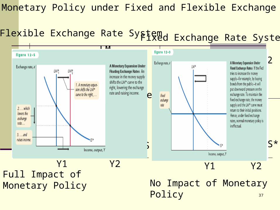
Impact of Monetary Policy under Fixed and Flexible Exchange Rate Systems
IS*
IS*’
e1
e2
Full Impact of Monetary Policy
LM LM1LM2
Fixed Exchange Rate System
Y1 Y2
e
IS*
Y1 Y2
Flexible Exchange Rate System
No Impact of Monetary Policy
38
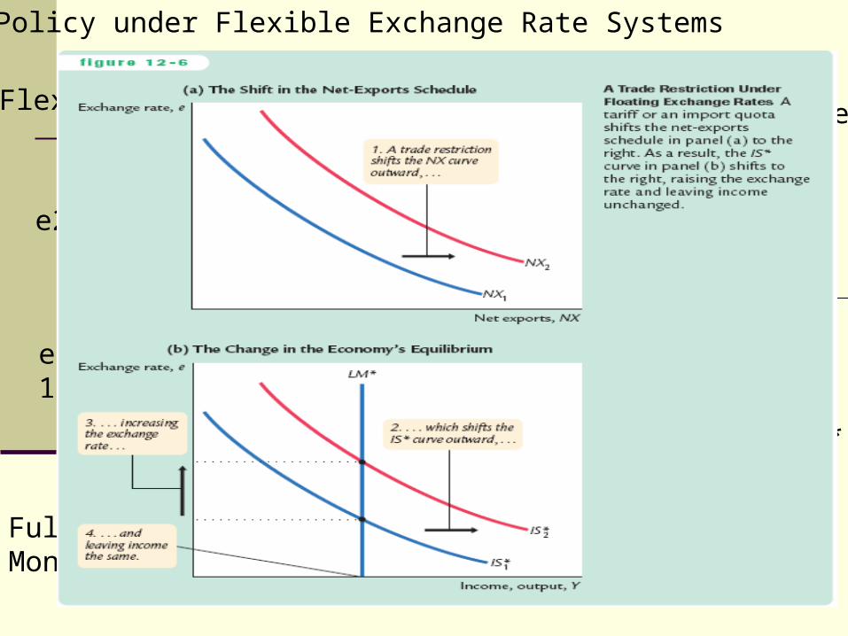
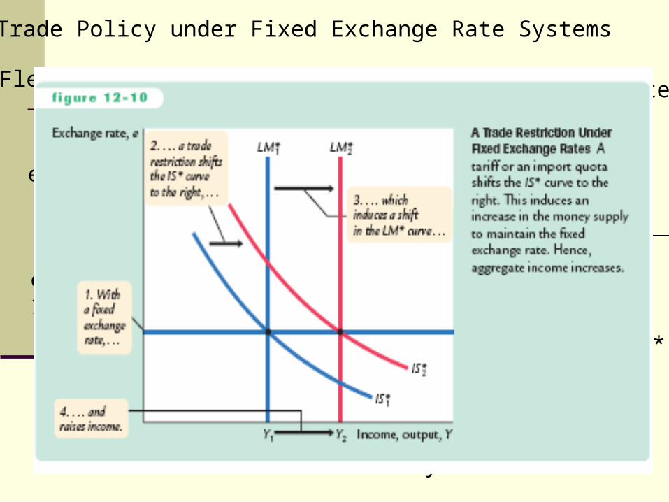
Trade Policy under Flexible Exchange Rate Systems
IS*
IS*’
e1
e2
Full Impact of Monetary Policy
LM LM1LM2
Fixed Exchange Rate System
Y1 Y2
e
IS*
Y1 Y2
Flexible Exchange Rate System
No Impact of Monetary Policy
39
Trade Policy under Fixed Exchange Rate Systems
IS*
IS*’
e1
e2
Full Impact of Monetary Policy
LM LM1LM2
Fixed Exchange Rate System
Y1 Y2
e
IS*
Y1 Y2
Flexible Exchange Rate System
No Impact of Monetary Policy

40
Determinants of Net ExportNet export function
eMXNX
eYeMeYXNX ,,*
NX = net exports X = exports e = nominal exchange rate M = imports Y* = income level in the foreign country Y = income level at home
Three sources of changes in net exports: 1. Exports 2. Imports and 3. Exchange rate

41
Marshall-Lerner condition Devaluation is effective if
1 mx ee
Devaluation is ineffective if
1 mx ee
Devaluation has no effect in trade balance
1 mx ee
xe is elasticity of export
me is the elasticity of imports

42
Change in net exports is zero if the sum of exchange rate elasticity of exports and imports equals 1. Net export increases if this sum is greater than one.
Net export decreases if this sum is less than one. Example: There is a devaluation
Export elasticity is 0.9 import elasticity if –0.8 Net export rises because 0.9-(-0.8) =1.7%.
Numerical Example of the Marshall-Lerner Condition

43
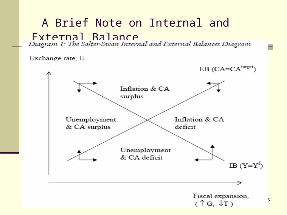
A Brief Note on Internal and External Balance
The Accounting Framework A major macro problem in the case of Africa/LDCs, is how to finance investment.
This may be addressed by starting from the national income accounting identity (eq. 1) and re-writing it to yield the accumulation balance (eqs. 2 and 3)
.
MXGICY
FMXIGCY NXMSISI ppgg )()(
NXMSIGTI ppctFiscalDefi
g
)(
pgppctFiscalDefi
g FFSIGTI
)(

44
A Brief Note on Internal and External Balance
Let us first consider the internal balance and how fiscal policy comes in the analysis. A superscript ‘f’ shows full employment level while ‘*’ shows foreign (as opposed to local/domestic) variables. ‘E’ and CA stand for nominal exchange rate and current account balance, respectively.
Assuming P* and E are fixed, inflation will depend on aggregate demand pressure which is strictly linked to the fiscal variables.
Internal balance requires that full employment holds (i.e. Aggregate demand equals aggregate supply at Yf ). This is give by 1st eqn.
.Coming to the external balance, if we assume that the government has a target level of current account balance (CAtarget), achieving this target requires 2nd eqn.
TY
P
EPfCAGITYfCY fff
*
ettf CATYP
EPfCA arg
*
,
45
A Brief Note on Internal and External Balance
46
References Blanchard (18) Mankiw (2) M&S (20) Bhattarai (2002) Welfare Gains to the UK from a Global Free Trade, European
Research Studies, vol. IV, Issue 3-4, 2001, pp55-72. pp. 1161-1176. Fleming J. Marcus (1962) Domestic financial policies under fixed and under
floating exchange rates, IMF staff paper 9, November , 369-379. Krugman Paul (1979) A Model of Balance of Payment Crisis, Journal of Money
Credit and Banking, 11, Aug. Krugman P. and L. Taylor (1978) “Contractionary Effects of Devaluation” Journal
of International Economics, 445-56. Miller, Marcus; Salmon, Mark When Does Coordination Pay? Journal of
Economic Dynamics and Control, July-Oct. 1990, v. 14, iss. 3-4, pp. 553-69 Mundell R. A (1962) Capital mobility and stabilisation policy under fixed and
flexible exchange rates, Canadian Journal of Economic and Political Science, 29, 475-85.
Sebastian E (1986) Are Devaluations Contractionary? Review of Economics and Statistics, vol. 68, 3, 501-508.
Taylor Mark (1995) The Economics of Exchange Rates, Journal of Economic Literature, March, vol 33, No. 1, pp. 13-47.
Whalley (1985) Trade Liberalisation among Major World Trading Areas , MIT Press for developments on trade arrangement among various trading regions.


