
On the Desired Rate of Capacity Utilization
Michalis Nikiforos∗
November 7, 2011
Abstract
This paper examines the endogeneity (or lack thereof) of the rate of
capacity utilization in the long run within the context of the controversy
surrounding the Kaleckian model of growth and distribution. We argue
that the proposed long-run dynamic adjustment, proposed by Kaleckian
scholars, lacks a coherent economic rationale. We provide economic jus-
tification for the adjustment of the desired rate of utilization towards the
actual rate on behalf of a cost-minimizing firm, after examining the fac-
tors that determine the utilization of resources. The cost minimizing firm
has an incentive to increase the utilization of its capital if the rate of the
returns to scale decreases as its production increases. We show that there
are evidence in the theory and the empirical research that justify this
behavior of returns to scale. In that way the desired rate of utilization
becomes endogenous.
JEL Classification Codes: B20, B50, D21, E11, E12, E22, E25
Keywords: Kaleckian, Long Run, Economies of Scale, Utilization
∗Department of Economics, New School for Social Research, 6 East 16th Street, NewYork, NY, 10003. I would like to thank Duncan Foley, Peter Skott, Lance Taylor, LucaZamparelli, Laura Barbosa de Carvalho, Christian Schoder and Jonathan Cogliano for usefulcomments and suggestions. The usual disclaimer applies. Financial support from the GreekState Scholarships Foundation is gratefully acknowledged.
Applicant upload/858,220/2011-11-10

1 Introduction
The Kaleckian model of growth and distribution is a standard analytical tool of
non-mainstream macroeconomics. The attractiveness of its theoretical frame-
work lies in the combination of the distribution of income and the existence of
classes with the principle of effective demand. In that sense, it is able to combine
the Keynesian emphasis on demand with classical ideas of political economy. Fi-
nally, it has the flexibility to accommodate different views and approaches, and,
as a result, it is no accident that it has been the field for many recent debates
among different economic traditions.
At the same time, the analytical framework of the model has been been
subjected to severe critique. The most fundamental argument of this critique is
that in the long run the rate of capacity utilization has to return to its normal,
desired or target rate. Since firms determine their desired rate of utilization
under the cost minimizing principle, there is no reason to change this desired
rate, unless the underlying reasons associated with the cost minimization prob-
lem change. The deviation of the actual rate from the desired rate is not one of
these. Therefore, the results of the Kaleckian model apply only in the short run.
In the long run we either have to find a way for the actual level of utilization to
adjust to the exogenous desired level (within the model’s framework), or aban-
don the model in favor of other formulations where—in the long run—the actual
level of utilization is equal to its exogenous desired level. Consequently in the
long run the Keynesian characteristics of the model cease to exist; there is not
space for the paradox of cost or the paradox of thrift. This critique is reinforced
by the Federal Reserve data, where the utilization of capacity gravitates around
a desired rate of around 80 percent.
The “Kaleckian side” has conceded that in the long run the two rates must
equalize. However they argue that it is the desired rate of utilization which
adjusts to the actual rate through the so-called hysteresis effect. Although this
argument is formally correct it lacks a coherent economic rationale.
The main contribution of the present paper is that it explains why a firm that
optimizes its behavior will tend to change its utilization in the face of a change
in the demand for its product. As we explained above, in the literature until
now the optimal desired rate of utilization has been thought to be exogenous.
Moreover, we are the first to argue that the Federal Reserve data on capacity
utilization—which has been used by both sides in this debate—are not appro-
priate for answering whether or not the desired of utilization is endogenous in
1
the long run.
The remainder of the paper is organized as follows. After a brief presenta-
tion of a stripped down version of the Kaleckian model, we examine the critique
against it and how the scholars supportive of the model have responded. Next,
we show that it is wrong to use the data of the Federal Reserve on capacity
utilization to examine long rung trends of the desired rate of utilization because
this series has no trend by construction. Therefore, the reported actual utiliza-
tion rate represents how much capacity is utilized compared to the desired rate
of utilization, but we cannot make any conclusion about the desired rate itself.
The only way to avoid this convention and see the long run trend of capacity
utilization is to examine the behavior of the average workweek of capital. In
that sense the full capacity is defined as 24 ∗ 7 = 168 hours per week. In section
6 we present several efforts to estimate the average workweek of capital, which
show that there has been an increase of the workweek of capital, and therefore
of utilization. If we look at the utilization of capital from this point of view, it
seems that it is far from stationary.
In section 7 we explore the factors that determine the optimal level of capac-
ity utilization by a firm. We show that the firm will tend to utilize its capital
more—adopt a double shift system—as the output grows, if there are increasing
returns to scale and the rate of the returns to scale decreases. In the following
section we examine how the theory of economies of scale can provide justification
for this kind of behavior of economies of scale.
Finally, in section 9 we put the pieces of the puzzle together and we show
how the desired rate of utilization becomes endogenous at the macro level.
2 The Basic Setup of the Model
The fundamental ideas of the Kaleckian model of growth and distribution go
back to the writings of the classical political economists, John Maynard Keynes
and—of course—Michal Kalecki (e.g.1971). In its contemporary form it has
been developed by Joseph Steindl (e.g. 1952), Rowthorn (1981), Taylor (1983,
1990, 2004), Dutt (1984, 1990), Amadeo (1986) and Marglin and Bhaduri (1990),
Bhaduri and Marglin (1990). It is worth noting that the model under exami-
nation and its broader analytical framework has received different names. Two
of the most common names within the literature are “Structuralist” and “Post-
Keynesian”.
2

Its basic setup is built around the concepts of demand and distribution. The
demand schedule is determined by the saving behavior of its members—workers
and capitalists—and the investment behavior of the firms. The total income of
the economy is distributed between wages and profits.
Investment (normalized for capital stock) can be defined as gi = I(π, u),
where π is the profit share, Y and Y is output and potential output respectively
and finally u = Y/Y is capacity utilization with Iπ > 0 and Iu > 01. The first
partial derivative explains the effect of a higher profit share on investment. For
Kalecki, higher realized profitability means higher profit expectations, which
have a positive effect on investment. Moreover higher profitability allows the
firm to finance a bigger part of its investment through internal funds and eases
the access to the capital markets. The effect of higher utilization on investment
is positive because firms want to hold excess capacity to face an unexpected rise
in demand, thus a higher degree of utilization will induce accumulation (Steindl,
1952). We can also think of this positive effect in terms of the acceleration
principle.
On the other hand, total saving (normalized for the capital stock) is gs =
S(π, u). Su is positive. The saving propensity of the capitalists is assumed to
be higher than the saving propensity of the workers and therefore Sπ is also
positive.
For the purposes of the present paper we will assume the following functional
form for the investment function
gi = γ + α(u − ud) + βπ (1)
where ud is the desired rate of utilization and α, β > 0. The only difference of
this formulation with the generic one above is that investment does not react to
the level of utilization per se but to the deviation of the level of utilization from
its desired rate for the same reasons outlined above. This kind of investment
function has been proposed by Steindl (1952) and Amadeo (1986) and more
recently has been used by Lavoie (1995, 1996) and Dutt (1997).
Moreover, for reasons of convenience, we will assume that the workers do
not save, and the saving behavior of the economy boils down to the familiar
Cambridge equation
gs = sr = sπρu (2)
1The subscript stands for the partial derivative for this variable.
3

where s is the saving rate of the capitalists, r is the profit rate and ρ = Y /Kip
is the ratio of the potential output to the capital stock in place.
The equilibrium level of utilization (u∗) will be such as to equate the total
saving and total investment gi = gs for the exogenously given distribution.
From equation (1) and (2) it is easy to see that
u∗ =γ − αud + βπ
sπρ − α(3)
and therefore the equilibrium level of the growth rate is
g∗ = sπρu∗ = sπργ − αud + βπ
sπρ − α(4)
The equilibrium is stable if sπρ > α, that is if savings react more than
investment to changes of utilization; what is usually called Keynesian stability
condition2.
From equations (3) and (4) we can see that the paradox of thrift holds, since
∂u∗/∂s and ∂g∗/∂s are both negative. On the other hand the effect of a change
in distribution to the level of utilization and growth depends on the relative
magnitude of the reaction of saving (Sπ = sρu∗) and investment (Iπ = β) to
changes in distribution. In our demand driven economy a decrease of saving
stimulates demand and thus output, while a decrease of investment decreases
demand and output. If saving reacts more than investment to a change in the
wage share (sρu∗ > β) a redistribution of income against capitalists will tend
to increase utilization and the growth rate. In this case ∂u∗/∂π and ∂g∗/∂π
are both negative. This is what is called a stagnationist, wage-led, or under-
consumptionist economy. If sρu∗ < β we are under an exhilarationist, profit-
led regime where the redistribution in favor of the capitalists leads to higher
output—∂u∗/∂π and ∂g∗/∂π are positive.
Aside from the demand schedule, where the distribution of income is the
exogenous variable, we can define the distributive schedule where the causality
runs in the other direction. The distributive schedule expresses how output
is distributed among wage and profit earners, and how distribution reacts to
changes in utilization. By definition the profit share share is equal to π = 1−ψ =
1− ωx , where ψ is the wage share ω is the real wage and x is labor productivity.
The question then is how these different components behave for different levels of
capacity utilization and how they interact and form the nominal wages, prices,
2For the equilibrium to make sense it must also be true that γ − αud + βπ > 0.
4
productivity and distribution. The answer to this question involves different
approaches to the macroeconomic debate.
A growing recent literature (e.g. Tavani et al., 2011, Assous and Dutt, 2010,
Nikiforos and Foley, 2011) examine the implications of a non-linear behavior
of distribution for different levels of utilization. However, in this paper we will
assume that the distribution of income is exogenously determined, hence
π = π = 1 − ψ (5)
Foley and Michl (1999) refer to this assumption as the Classical conventional
wage share, due to the view held by the classical economists that the distri-
bution of income—at least in the long run—is exogenously determined at the
subsistence level of the workers (which in turn is conventional).
The equilibrium level of distribution and capacity utilization is the outcome
of the interaction of the demand and the distributive schedules, “the functional
distribution of income and effective demand jointly determine economic activ-
ity” (Foley and Taylor, 2006, p.75). As a result of the exogenous distribution
assumption, the impact of a change in distribution on utilization and growth
can be inferred by equations (3) and (4).
3 The controversy around the Kaleckian model
3.1 The critique
The Kaleckian model has been criticized on many levels. For example Skott
(2008a,b) questions the assumption that saving reacts more than investment to
changes of income, what we called Keynesian stability condition, and Steedman
(1992, p.125) poses some “questions concerning the Kaleckian theory of pricing
and the closely related theory of distribution”.
However, the most persistent critique is related to the inability of the Kaleck-
ian model to equate the actual rate of capacity utilization (u∗) with the ex-
ogenously given desired—or normal or planned—rate (ud). Committeri (1986,
p.170), referring to the contributions of Rowthorn (1981) and Amadeo (1986)
writes that “there is the possibility of utilization being different from its normal
degree, even in states of equilibrium (and indeed, actual and normal utilization
would coincide only by a mere fluke).” Auerbach and Skott (1988, p. 52) claim
5

that a steady growth path with u∗ #= ud is ruled out, i.e. u∗ = ud along the
steady growth path3” and they add in the next page that “it is inconceivable
that utilization rates should remain significantly below the desired level for any
long period”.
The failure of the Kaleckian model to equate the actual to the desired rate of
capacity utilization has led many to consider it as relevant only in the short run.
For example Dumenil and Levy (1993) provide a mechanism for the convergence
of the economy from the short term Keynesian/Kaleckian equilibrium “with any
capacity utilization rate” to the long run classical equilibrium “with a normal
capacity utilization rate”.
Heinz Kurz (1986) explores the concept of the normal rate of utilization.
Quoting Sraffa (1960) he argues that the normal rate of utilization “will be
exclusively grounded on cheapness”. In other words, each firm will chose how
much to utilize its capital based on the principle of cost minimization. Kurz
uses the example of a firm that can produce a certain amount of output either
by employing a certain amount of capital and labor in a single-shift mode of
operation, or by employing a second shift and using only half the capital. The
wage of labor in the second shift is higher than in the first because of social
norms and conventions (e.g. the wage premium earned by workers who work
during the night). The firm will choose the system of operation—and thus
the level of utilization of capital—which is more profitable (or which is less
costly). Under Kurz’s setup the level of the normal rate qualifies as exogenous
and structurally given. Utilization will only change in response to technological
changes or changes in the norms that determine the relative cost of labor between
the two shifts.
In conclusion, the critique can be summarized in the following arguments:
i) in the long run utilization cannot be different from its desired rate, ii) the
desired rate is determined on the basis of the cost-minimizing principle and iii)
the desired rate for a firm that minimizes its cost is exogenously given. Thus—in
the long run— the rate of utilization gravitates around a structurally given and
exogenous desired rate of utilization. The critique is serious. If it is correct, the
conclusions of the model are only short-run. In the long term, we either have
to turn back to the classical results, where there is no room for the paradox
of thrift and the paradox of cost—a higher saving rate leads to higher growth
and a lower real wage and wage share is always related to lower profit rate and
3Auerbach and Skott (1988) use u and u∗ to symbolize the actual and the desired rate ofutilization respectively. The change has been made for reasons of consistency.
6

growth—or we have to seek other formulations which can potentially establish
Keynesian results. Committeri (1986) and Dumenil and Levy (1993) are in favor
of the first approach while Skott (2008a,b) support the latter.
3.2 The Kaleckian response
In response to this critique the proponents of the Kaleckian model have argued
that in the long run it is the desired rate of utilization that converges towards
the actual rate and not the other way around. Amadeo (1986, p.148) says “we
should be prepared to examine the possibility of utilization being an endogenous
variable even in the long period”. A few pages later (p. 155) he adds: “ Indeed
one may argue that if the equilibrium degree is systematically different from the
planned degree of utilization, entrepreneurs will eventually revise their plans,
thus altering the planned degree. If, for instance, the equilibrium degree of
utilization is smaller than the planned degree (u∗ < ud), it is possible that
entrepreneurs will reduce ud”4.
More formally, what he proposes is an adjustment process described by the
following dynamic equation
ud = µ(u∗ − ud) (6)
where µ > 0 and ud is the derivative of ud with respect to time.
In a series of articles Lavoie (1995, 1996), Lavoie et al. (2004) and more re-
cently Hein et al. (2010) are more explicit. They argue that the firms apart from
the capital/capacity they own and they operate according to the principle of cost
minimization—as described by Kurz (1986)—have “some plants or segments of
plant [that] remain idle in normal positions”(Lavoie et al., 2004, p.133). This
kind of complete idleness of a part of capital is maintained by firms in order to
face the uncertainty of future demand. They conclude (in the same page) that
“the normal rate of capacity utilization, in that context, is thus a convention
[emphasis added], which may be influenced by historical experience or strategic
considerations related to entry deterrence. Although firms may consider the
normal rate of capacity utilization as a target, macroeconomic effective demand
effects might hinder firms from achieving this target, unless the normal rate is
itself a moving target influenced by its past values”(Lavoie et al., 2004). Similar
arguments, with such a distinction of capacity between capacity that is oper-
4Amadeo (1986) uses un for the planned degree of utilization.
7

ated under the principle of cost minimization and capacity that stays idle as a
buffer for a potential future increase in demand can be found in all the papers
mentioned before, authored or co-authored by Marc Lavoie.
Finally, Amitava Dutt (1997, p.247) explains the endogeneity of the desired
rate of utilization in terms of “strategic considerations of the firms”. The firms
will reduce their desired utilization rate if they “expect a higher rate of entry
than at present” and they consider the entry threat to be “proportional to the
investment rate”, thus ud = µ′(g0 − g∗), which with the help of equations (1),
(3) and (4) can be transformed into equation (6)5.
Based on this interpretation equations (3) and (4) define a short run equi-
librium, where the desired rate of utilization is exogenous. In the long run the
desired rate becomes endogenous and behaves according to equation (6). To
“close” the system Lavoie (1995, 1996) and Dutt (1997) supplement equation
(6) with the following dynamic equation
γ = θ[g∗ − (γ + βπ)] (7)
where γ + βπ represents the expected rate of accumulation and θ > 0. If the
actual rate of accumulation exceeds the expected rate firms revise their expec-
tations about the growth rate upwards; an argument with intense Harrodian
flavor6. This dynamic equation can be rewritten as
γ = θ[a(u∗ − ud)] (8)
Equations (6) and (8) define a 2 × 2 system of dynamic equations. Substi-
tuting the equilibrium values of utilization it becomes
ud = µ(γ−αud+βπsπρ−α − ud)
γ = αθ(γ−αud+βπsπρ−α − ud)
(9)
An extensive analysis of this system is beyond the scope of this paper. In
brief, the Jacobian of this system is zero. For stability, it is required that the
trace of the Jacobian is negative, that is µsπρ > αθ. The sufficient condition
for this to hold—because of the Keynesian stability condition—is µ > θ, that
is the adjustment of the desired utilization rate is faster than the adjustment
of the desired growth rate. The system has an infinite number of equilibria.
5Implicitly it is assumed that g0 = γ + βπ.6See Harrod (1939).
8
The steady state depends on the initial equilibrium and the path of economy
towards it.
The important feature of this formulation is that the economy remains de-
mand driven in the long run: the paradox of thrift and the paradox of cost
continue to hold. A higher saving rate will lead the economy to a steady state
with a higher level of utilization and growth rate. Interestingly, in the long run
the economy cannot be profit-led. A higher profit share decreases the steady
state level of utilization and growth.
3.3 Why the response is unconvincing
From a formal point of view the arguments of the preceding section answer the
critique regarding the impossibility of a long run deviation of the actual rate
of utilization from the desired one. The actual and the desired rate are equal
in the long run. However, they fall short in explaining why the desired rate of
utilization behaves in the way it is described in equation (6). Stated differently,
why a deviation of the actual utilization from the desired rate would induce the
entrepreneurs to revise their desired rate? It is not clear why in the long run
a firm will desire a lower level of utilization in response to a recession and vice
versa.
The argument of the conventional desired rate of utilization is not convincing
for two reasons. First, there is no particular rationale behind distinguishing
excess capacity in the form of lower than full speed of operation, or lower than
full time of operation (one shift instead of two or three shifts), or in the form of
totally idle capacity, of “some plants or segments of plant remain[ing] idle”. If a
firm operates at 80% of capacity in order to be able to respond to an unexpected
increase in demand or to deter the entry to possible competitors7 it can do it
either by lowering the speed of its operation to 80% of what it would be, or
by operating its plants 80% of the time it would otherwise operate them, or
by keeping a 20% of its productive capacity idle, or by a combination of all
three of them. There is no general a priori reason—theoretical or based on the
actual experience—that makes the last method superior to the two first. Under
certain certain technologies it would probably be more profitable for the firm to
choose the idleness method, but this would depend on certain characteristics of
an industry and is not a general rule. On the contrary we could think of reasons
7The argument of low utilization as an entry deterrence mechanism is made by Spence(1977).
9
why the firm would favor the first two methods compared to the third one (e.g.
adjustment costs for hiring labor).
Moreover, even if this claim were true, the utilization rate does not become
a convention. The need of the firm to face unexpected increases in demand is
an objective and non-conventional reason for keeping a part of its capacity idle.
A behavior of the desired utilization rate as described in equation (6) based on
the need of the firm to face unexpected demand, would mean that when the
actual rate of utilization is lower than the desired rate, the firm expects more
volatile demand and thus decreases its desired rate of utilization, but it is hard
to see why this would happen.
4 Capacity and Capital utilization
Before proceeding to the analysis of the thesis of this paper it would be useful
to open a parenthesis and discuss briefly the concept of capacity utilization and
then its relation with capital utilization.
The difficulty with the concept of capacity utilization arises because of the
ambiguous meaning of capacity. How can one define capacity? Different answers
have been given to this question. The most straightforward definition of capacity
is the engineer capacity, the maximum level of output obtained if we use the
quasi-fixed factors of production 24 hours per day and 7 days per week at the
maximum possible speed of operation. The full capacity of a firm whose only
quasi-fixed production factor is a factory is the output that would be produced
if this factory was working 168 hours per week at full speed. We can also define
a statistical concept of capacity. This is usually done by deriving a peak-to-peak
trend of output or applying a filter (e.g. Hodrick and Prescott, 1997) to the
time series of output.
Besides these two concepts, we can define capacity as an economic (as op-
posed to engineer or statistical) concept. Two alternative definitions have been
employed. As preferred capacity, it is usually defined the level of capacity spec-
ified with the cost-minimization principle. On the other hand practical capacity
(or full production) is defined as the level of production where the variable (non-
quasi-fixed) inputs are used at their maximum level. These definitions are not
identical but are close both from a theoretical and an empirical point of view.
In the next section we show that the change in the questionnaires of the Census
from the one definition to the other led to a small discrete change in the re-
10
ported utilization (around four percentage points)8. These definitions are close
to what we have called desired or normal utilization.
Within the context of these definitions the importance of the distinction be-
tween capacity and capital utilization becomes more clear. Many times the two
terms are used interchangeably with or without always realizing it. However,
we should note that there are important differences between them. The utiliza-
tion of capital expresses how much of the capital stock, as a distinct input of
production, is utilized, while capacity utilization measures how much output is
produced vis-à-vis how much output could be produced. Capital and capacity
utilization would be the same only if capital is the only quasi-fixed factor of
production.
In this paper we will not make a distinction between the two concepts. In
other words we will assume that capital is the only quasi-fixed input in pro-
duction. With a Leontief-type production function and with the assumption of
elastic supply of labor, an assumption almost universal in the related literature,
the ratio of potential output to capital in place is equal to the ratio of capital
services (or utilized capital) to actual output. As a result Y /Kip = Y/Ks, so
the two definitions of utilization coincide (Ks stands for the capital services).
Therefore in the series of articles and books which discuss the issue of the long
run rate of actual and desired utilization, explicitly or implicitly, the two defi-
nitions are used interchangeably. We will follow the same path but we should
keep in mind the difference between the two and the prerequisites for their
coincidence.
5 Data on Utilization
5.1 The Federal Reserve Data on Utilization
The Federal Reserve Board (FRB) data on capacity utilization have been used
by both sides in the debate9. Lavoie et al. (2004) filter the data with the
Hodrick-Prescott (HP) filter and they argue that the fluctuations of the HP-
filered series prove that the desired rate adjusts as described in equation (6).
They provide an econometric justification for their claim using these data10.
8A detailed discussion of the different definitions is provided among others by Klein (1960),Berndt and Morrison (1981), Morrison (1985), Bresnahan and Ramey (1994), Mattey andStrongin (1997) and Corrado and Mattey (1997).
9The data can be found at http://www.federalreserve.gov/releases/g17/caputl.htm10They use data on capacity utilization from Statistics Canada, which are practically the
same with those of the FRB
11

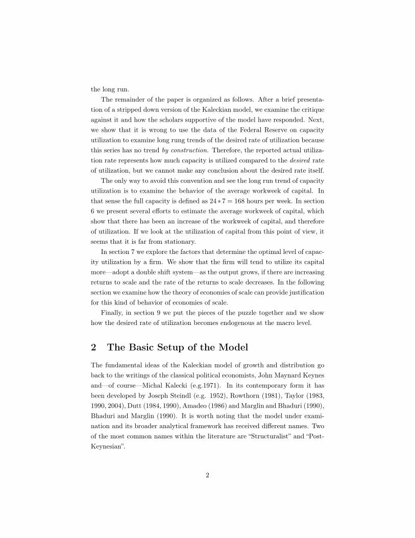
In figure 1 we present the FRB capacity utilization series for the US economy
for the period 1948 to 2007. It is hard to see how these data support the claim
of an endogenous utilization rate. From the fitted lines it becomes obvious
that the rate of capacity utilization tends to gravitate around a constant rate
over a prolonged period of time, around 83% in the period 1948 to 1980 to
around 79% in the period 1980 to 2007. This change can be attributed to a
change of the structural characteristics behind the desired rate of utilization.
For example, Spence (1977) would argue that this shift is the result of an increase
in the concentration in the market and as a result the firms need to lower their
utilization rate to deter the entry of the competitors. However, we do not
have to go that far. Morin and Stevens (2004, p.9), in a paper describing the
construction of the FRB capacity utilization index11, argue that a big part—if
not the whole—of this decrease is due to changes in the definition of capacity in
the questionnaires of the surveys which are used to construct the index. These
changes led to a “discrete shift” of the index around “4 percentage points”. It is
probably no coincidence that this is the difference between the two horizontal
fitted lines.
Similarly, in the case of the HP filtered series of utilization, we observe a
remarkable stability of the desired rate of utilization—if we interpret the HP-
series as representing the desired rate. Over the whole period there are some
minor fluctuations, but they are not enough to support the hypothesis of an
endogenous rate of utilization. If we HP-filter the series for the period before
and after 1980 we will end up with almost horizontal lines, as in the case of the
linear fits, which, taken together with the change of the estimated utilization
rates because of the questionnaire, leads to the conclusion of a constant desired
rate of utilization.
Therefore, if one relies on the capacity utilization index of the Federal Re-
serve, the argument of an endogenous rate of capacity utilization seems unwar-
ranted. Instead, there seems to exist an exogenous desired rate of about 80%,
around which the actual rate gravitates.
However, the FRB data is inappropriate to judge whether the desired rate
of utilization is (or is not) endogenous in the long run. This becomes clear
if we pay a little closer attention to the way these data are constructed. For
that purpose the paper by Morin and Stevens (2004) is very useful. The index
is based on the Survey of Plant Capacity (SPC) which is conducted by the
11The online documentation of the Industrial Production and Capacity Utilization in thewebsite of the Federal Reserve (2009) is a short version of this paper.
12

Figure 1: Capacity Utilization from the FED dataset. Annual data, for theperiod 1948-2007.
United States Census Bureau12. In the questionnaires of the SPC the plant
managers are asked to specify the “full production capability of their plant—the
maximum level of production that this establishment could reasonably expect
to attain under normal and realistic operating conditions fully utilizing the
machinery and equipment in place”. Among the instructions they are given
is to “assume number of shifts, hours of plant operations, and overtime pay
that can be sustained under normal conditions and a realistic work schedule13”.
The results of this questionnaire are then processed and aggregated in order to
produce the series we present in figure 1.
Let us put ourselves in the shoes of a plant manager who answers the ques-
tionnaire. Assume that over a period of years our plant works 5 days per week,
8 hours per day. Under these normal and realistic conditions the number of
shifts is one and the hours of plant operations per week is forty. We can also
assume that the full production capacity of the plant under these normal con-
ditions is 100 units. The plant manager wants to be able to face unexpected
12A copy of the questionnaire can be found online athttp://bhs.econ.census.gov/bhs/pcu/pdf/10_mqc2.pdf
13Emphasis in the original.
13

demand increases (or to deter the entry of the competitors in the market), so
the plant is working on average at the 80% of its full capacity. Note that there
is no general reason why the manager either does not “run” the plant at its full
speed, or lets the workers go home earlier, or keeps a part of the plant idle.
Therefore, on average the production of the plant will be 80 units vis-à-vis a
full production capability of 100 units, that is utilization of capacity around
80%. Of course when the economy is doing well and the demand is high the
plant manager will increase the speed of production, or will not let the workers
leave earlier—they might even work overtime—or he will utilize the idle part of
the plant. In these “fat cow” years, when he fills the SPC questionnaire the pro-
duction will be higher than 80 units and therefore the utilization will be higher
than 80%. In years of economic downturn for the same reasons the utilization
will be lower than 80%.
Imagine that our firm is doing well and after a period of high demand the
plant manager decides to add a second shift. Over a period of years the plant
works 5 days per week, 16 hours per day. Under the new normal and realistic
conditions the number of shifts is two and the hours of plant operations per week
is eighty. The full production capability of this plant under the new normal
conditions is 200 units (we abstract from any kind of economies of scale or
other reasons that would make this product to be different than 200). The
plant manager still worries about competition and being able to face unexpected
demand. That is why he “runs” his plant on average at the 80% of its full
capability. Therefore, on average the production of the plant will be 160 units
vis-à-vis a full production capability of 200 units, that is utilization of capacity
around 80%. The cyclical fluctuations effects still apply and have the same
effects.
If after a few years the demand for the products of the firm permanently
decreases and the manager decides to drop the second shift, we will be back to
the original situation
The conclusion of this simple example is that the FRB index of capacity
utilization by construction gravitates around a structural exogenous level of
utilization and by construction is stationary. In the online documentation of
the Federal Reserve (2009) it is made explicit that “a major aim is that the
Federal Reserve utilization rates be consistent over time so that, for example,
a rate of 85 percent means about the same degree of tightness that it meant in
the past”. In that sense the FRB utilization index is a proxy for the deviation
of u∗ from ud and gives us no information about the ud itself.
14
In order to examine the behavior of the utilization over the long run we have
to rely on other measures, which can capture if the plant “runs” for one or two
(or three) shifts, if it runs during the weekends etc. The obvious method to do
that is to compare the number of hours the plant works with the maximum hours
it can work. The maximum hours the plant can work within one week period
is 24 × 7 = 168 hours. Therefore, a more appropriate measure of utilization for
our purpose is the ratio of hours worked by the plant per week over 168. In
that case the utilization of our fictional plant of the previous paragraphs would
have increased from an average of 80% ∗ 40/168 % 20% to 80% ∗ 80/168 % 40%.
As we will see in the next section this measure is not without problems but it
is more appropriate for our discussion. In the next section we present various
attempts to measure utilization, which capture the amount of time the capacity
is utilized.
6 Other Measures of Utilization
A first attempt of measuring capital utilization as the ratio of the time the
plant worked over an absolute amount of time (number of hours per week or
year) was made by Foss (1963). He used data on power equipment from the
Census of Manufactures and estimated the theoretical maximum of electrical
consumption of the machinery-in-place for a one-year period. He then estimated
the utilization rate of the machinery by comparing this theoretical maximum
to the actual consumption of electricity(available from the Census of Mineral
Industries). Foss finds that the “equipment utilization ratio from 1929 to an
approximately comparable high employment year in the 1950’s [1955] shows an
increase of almost 45%”. Foss’ methodology has several drawbacks related with
the assumptions he made to estimate his theoretical maximum. However two
main conclusions, which would be confirmed by later studies, came out: i) the
capital equipment lies idle most of the time and ii) there is a clear upwards
trend in the utilization of capital equipment.
Foss (1981a,b) uses a more direct method. He utilizes data from the 1929
Census of Manufactures and the 1976 Survey of Plant Capacity undertaken
by the Census Bureau on weekly plant hours worked by manufacturing plants,
which he then aggregates. The results are summarized in table 1. We can see
that over the period 1929 to 1976 the average workweek of capital increased
around 25 percent. If we take into account that 1929 was a year at the peak of
15

Variant 1929 1976 Change(%)
Aa 66.5 81.8 23.0
Bb 91.9 110.3 20.0
Cc — — 24.7
Source: Foss (1981a,b)aHours for each industry (at a four and two digit level) weighted by employment in each year.bHours for each industry (at a four and two digit level) weighted by capital in each year.cHours for each industry at the four digit level constructed as in B and aggregated using as
weights the gross fixed capital stock for 1954 in 1972 prices.
Table 1: Alternative measures of average weekly plant hours in manufacturingand their change, 1929 to 1976
the economic cycle while 1976 was close to the bottom the increase is higher.
Foss stresses that this increase occurred in the face of a decline in the average
workweek of a labor “from a customary 50 hours per week in 1929 to a 40-hour
standard in 1976”.
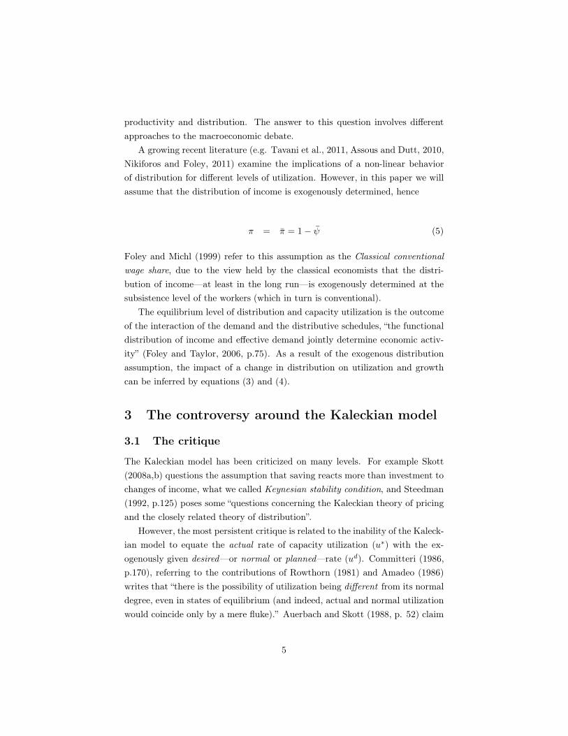
In a later study Foss (1984) makes use of the Area Wage Surveys of BLS,
covering metropolitan areas for high employment periods, 1959-60, 1969 and
1978-79. The percentage of workers employed on second and third shifts for
all manufacturing industries combined is used to interpolate the average weekly
plant hours (of table 1). The estimates between “pairs of endpoints” is derived
by straight line interpolation. Thus the annual estimates between 1929 and
1976 constitute a “high employment trend-line”. The results are presented on
the left hand side of the dashed line in figure 2.
Certain industries, because of some particular characteristics of theirs, usu-
ally either work only one shift (like apparel), or 3-shift (like Petroleum). The
latter are usually called continuous industries. The continuous (24 hours a day)
utilization of the capital in these industries is usually related to very high costs
of stopping and restarting production. Foss finds that if we excluded these
two types of industries the increase in average weekly plant hours reaches 32.4
percent between 1929 and 1976.
Finally Foss (1995) is able to construct annual indices based on actual annual
observations of utilization for the period 1976 to 1988. The results are depicted
on the right hand side of the dashed line of figure 2. The series presents the
expected cyclical fluctuations.
The Average Workweek of Capital (AWW) has been also estimated by other
16

Figure 2: Index for the average workweek of capital in manufacturing(1929=100) based on Foss (1984) and Foss (1995).
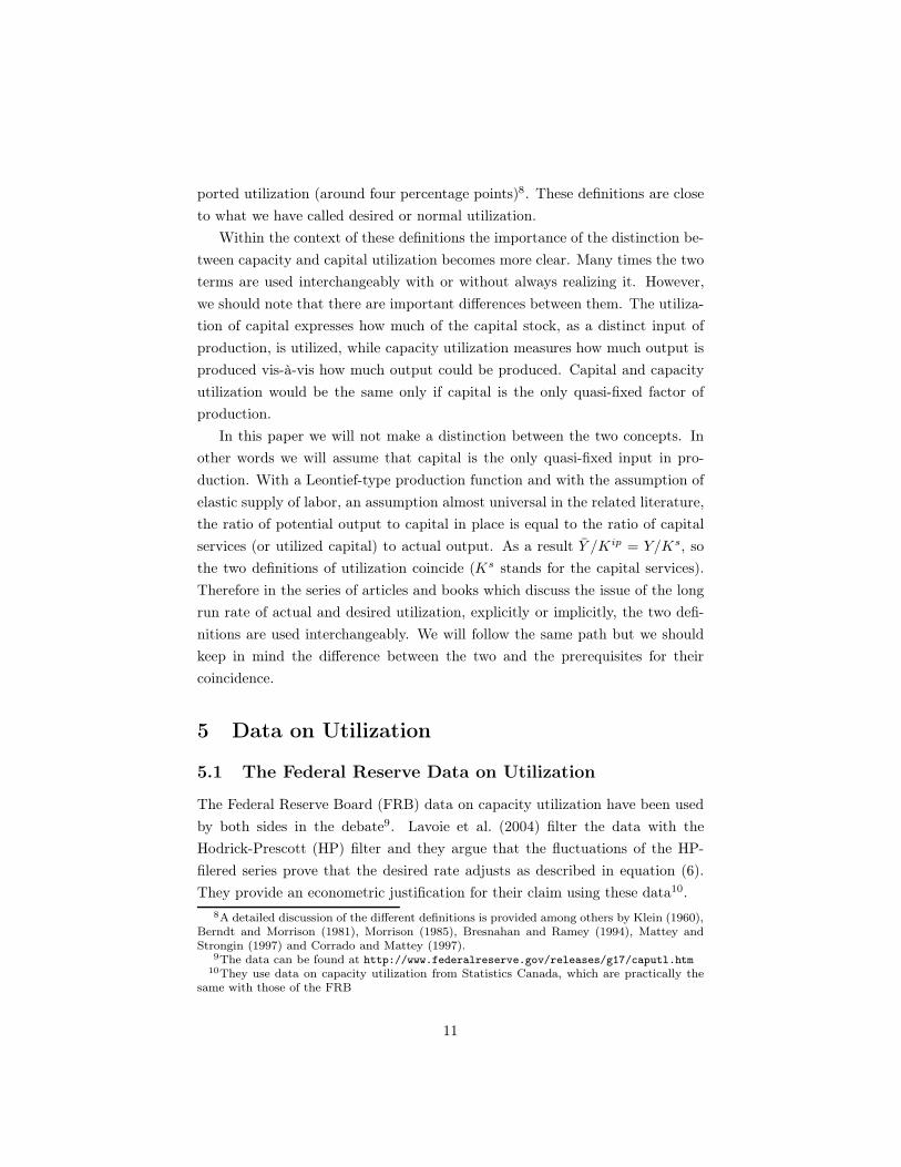
researchers. Taubman and Gottschalk estimate AWW for the period 1952 to
1968. The logic behind their effort is that the amount of the services of the
capital stock can change either by varying the speed of operation or by varying
the time the capital stock operates. Assuming that the speed of operation
remains constant, the most common method of altering the time of operation
of the capital stock is by changing the number of shifts it operates. Therefore,
the amount of capital services can be estimated using the information of how
many workers are employed in each of the three shifts14. Orr (1989), using the
same methodology, extends the estimation for the period until 1984.
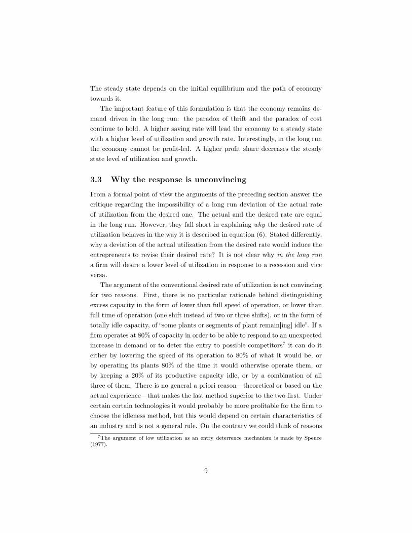
Their estimates are presented in figure 3a. It is clear that the utilization
of capital presents pro-cyclical fluctuations and that there is a definite upward
trend of the utilization of capital. Both papers run simple linear regressions and
find statistically significant positive trends.
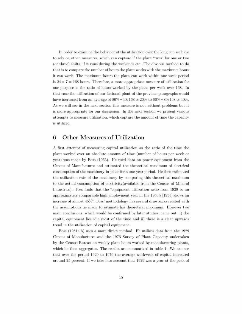
The same methodology is also followed by Shapiro (1986) for estimating the
average workweek of capital for the period 1952 to 1982. He follows Taubman
and Gottschalk until 1968. For the period 1969 to 1982 he is using his own
estimates of national level data on shift-work and the workweek of labor. As a
14The necessary data come from the Area Wage Surveys of the Bureau of Labor Statistics.
17
(a) Index for the average workweek of capital in manufacturing (1966=100) based on
Taubman and Gottschalk (1971) and Orr (1989).
(b) The average workweek of capital in manufacturing (1952=100) from Shapiro (1986).
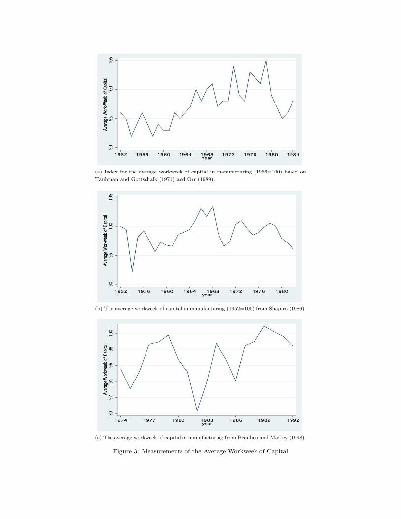
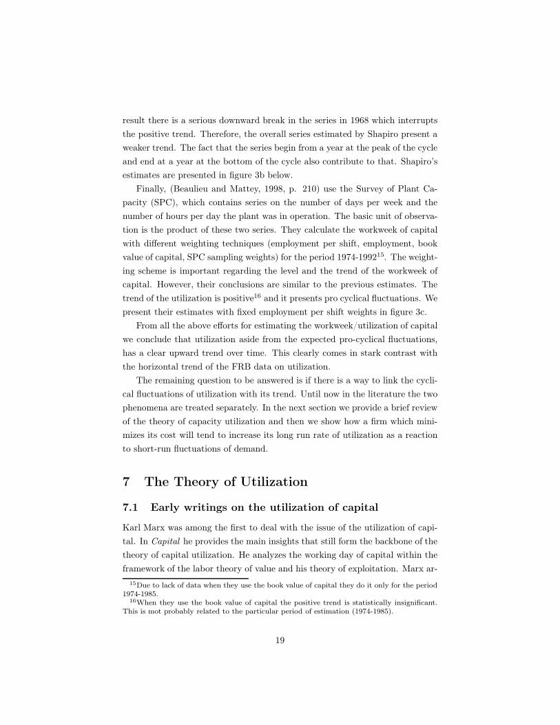
(c) The average workweek of capital in manufacturing from Beaulieu and Mattey (1998).
Figure 3: Measurements of the Average Workweek of Capital
result there is a serious downward break in the series in 1968 which interrupts
the positive trend. Therefore, the overall series estimated by Shapiro present a
weaker trend. The fact that the series begin from a year at the peak of the cycle
and end at a year at the bottom of the cycle also contribute to that. Shapiro’s
estimates are presented in figure 3b below.
Finally, (Beaulieu and Mattey, 1998, p. 210) use the Survey of Plant Ca-
pacity (SPC), which contains series on the number of days per week and the
number of hours per day the plant was in operation. The basic unit of observa-
tion is the product of these two series. They calculate the workweek of capital
with different weighting techniques (employment per shift, employment, book
value of capital, SPC sampling weights) for the period 1974-199215. The weight-
ing scheme is important regarding the level and the trend of the workweek of
capital. However, their conclusions are similar to the previous estimates. The
trend of the utilization is positive16 and it presents pro cyclical fluctuations. We
present their estimates with fixed employment per shift weights in figure 3c.
From all the above efforts for estimating the workweek/utilization of capital
we conclude that utilization aside from the expected pro-cyclical fluctuations,
has a clear upward trend over time. This clearly comes in stark contrast with
the horizontal trend of the FRB data on utilization.
The remaining question to be answered is if there is a way to link the cycli-
cal fluctuations of utilization with its trend. Until now in the literature the two
phenomena are treated separately. In the next section we provide a brief review
of the theory of capacity utilization and then we show how a firm which mini-
mizes its cost will tend to increase its long run rate of utilization as a reaction
to short-run fluctuations of demand.
7 The Theory of Utilization
7.1 Early writings on the utilization of capital
Karl Marx was among the first to deal with the issue of the utilization of capi-
tal. In Capital he provides the main insights that still form the backbone of the
theory of capital utilization. He analyzes the working day of capital within the
framework of the labor theory of value and his theory of exploitation. Marx ar-
15Due to lack of data when they use the book value of capital they do it only for the period1974-1985.
16When they use the book value of capital the positive trend is statistically insignificant.This is mot probably related to the particular period of estimation (1974-1985).
19

gues that since the (fixed) capital exists in order to “absorb labor and, with every
drop of labor, a proportional quantity of surplus labor...Capitalist production
drives, by its inherent nature, towards the appropriation of labor throughout
the whole of the 24 hours in the day. But since it is physically impossible to
exploit the same individual labor-power constantly during the night as well as
the day, capital has to overcome this obstacle. An alteration becomes necessary,
between the labor-powers used up by day and those used up by night”(Marx,
1976, ch. 10, p.367).
Thus the shift system is the means which allows the capitalists to appro-
priate surplus value throughout the 24 hours. A careful interpretation of this
would lead to the conclusion that the working day of capital is determined
by the capitalists—given the established norms of the working day and the
technology—in their effort to maximize the surplus value or the rate of the
surplus value.
The working day is a recurrent theme in Marx’s work, always in relation
to the his theory of production of surplus value17. However, the distinction
between the working day of capital and labor is not always explicit.
John Stuart Mill (1864, ch. IX, p.176) in his Principles of Political Economy
argues that “the only economical mode of employing” the machines is to keep
them “working through the twenty-four hours18”. Kurz (1986, p.42) interprets
this statement as Mill arguing that the firm under the profit maximizing prin-
ciple will run its machines through the twenty-four hours and therefore “Mill’s
opinion cannot be sustained”. It is more probable that the meaning of this
short comment by Mill is that the machinery is wasted if it is not utilized and
this waste is non-“economical”. A century later Georgescu-Roegen (1972, p.
284) stresses—along the same lines—that capital “idleness is the worst form of
economic waste and a great hamper to economic progress”.
Finally, the young Alfred Marshall in the essay The Future of the Working
Classes Marshall (1925)19 argues that society would benefit from the “diminu-
tion of hours of manual labor”. He recognizes that “for every hour, during which
17For example in chapter 15 of Volume 1 of Capital he examines the working day in relationto the introduction of the machinery in production. In the same chapter (p. 533-544) Marxdeals with the speed of production, which as we will see below, is another constituent of themodern theory of utilization of capital.
18In this chapter Mill discusses the “Production on large and production on a small scale”.He comments a passage of Charles Babbage’s On the economy of machinery and manufactures
(1832, p.174) and explains that the larger the scale production “the further the division oflabor may be carried”.
19The essay was written and originally published in 1873.
20

his untiring machinery is lying idle, the capitalist suffers loss” (p. 113). The
solution he proposes is the adoption of the multiple shift system, so as both the
working day of labor is short and the capital does not sit idle. Note that the idea
of idle capital as a form of economic waste is also present in this argument of
Marshall. In his last book, Industry and Trade (1920) he reflects on the British
society and the “place of Britain in the world” after World War I. He argues
in favor of extracting “as much work as possible out of his plant”. Again his
proposal is “to work in shifts, so as to keep the plant at work for twice as long
as the normal working day, then wages will be raised automatically far above
their present level”.
7.2 Recent contributions to the theory of capital utiliza-
tion
The insights provided in these early writing have become more explicit in more
recent contributions, which examine the determination of capital utilization.
The problem of the choice of the optimal utilization on behalf of a firm is
similar in nature with the more familiar choice of the capital labor ratio. For
example, the choice of the optimal capital-labor ratio is related (among others)
to the trade-off between increasing labor productivity and decreasing capital
productivity as we move from one capital labor ratio to the other20. Similarly,
the choice of the level of capital utilization is related to the trade-off between
the lower total capital cost of a higher level of capital utilization and the higher
wage which is required as a compensation for working non-normal hours.
The similarity of the two problems was recognized by Marris (1964). He
says (p.5) “We may therefore restate the production function by saying that
annual output now depends on three variables in place of two: instantaneous
employment, quantity of capital and the rate of utilization”. In the traditional
production theory the firm has to choose only the optimal capital-labor ratio.
Implicitly this is tantamount to assuming that the utilization of capital is al-
ways maintained at a constant level. Therefore capital utilization adds “another
dimension” to the choice problem of the firm. This second dimension can be
thought of either in continuous terms, e.g. how much time during a day capital
is utilized, where time is a continuous variable (this is the approach used by
20A necessary condition for that is the set of techniques of production and the productionfunction to be “well-behaved”, in the sense that higher capital productivity is accompaniedwith lower labor productivity. The production function as the description of the existence ofinfinite well behaved techniques is explained in Foley and Michl (1999).
21

Georgescu-Roegen, 1969, 1970, 1972), or in discrete terms. In the second case,
how a firm chooses the number of shifts it operates. This approach is followed
by both Marris (1964) and Betancourt and Clague (1981).
Therefore, the question is what are the factors that determine the level of
utilization. A standard approach within the literature is to distinguish the fac-
tors which are related to cyclical fluctuation and others which are not. Winston
(1974b) says “idle capital is explained as a consequence of unwanted accidents
and adversities that occur after [ex post] a plant is built, or as a result of ra-
tional ex ante investment planning”. In Marris’ words it is “methodologically
convenient to distinguish” between them. This approach, at least at a first sight,
is in accord with the critics of the Kaleckian model that there is a set of factors
that determine the long run, ex ante, desired level of utilization and another set
of factors that explain the short run, ex post, actual level.
The ex post unwanted utilization is usually explained in terms of cyclical
fluctuations in demand (Winston (1974b) is actually using the word “Keyne-
sian”), unexpected shocks or simply to mistakes of judgement on behalf of the
entrepreneurs. Therefore, the literature is mostly concerned with the factors
that determine the ex ante level of utilization.
However, as we will see later, no matter how convenient it is to distinguish
the two sets of factors, there is not always a clear cut way to do that and, as a
result, the ex post level of utilization is also related to the actual level.
7.3 The Ex Ante Decision on Capital Utilization
The literature on capacity utilization is well summarized by Winston (1974b). In
his article he mentions a series of determinants of the optimal capital utilization,
ex ante. A first reason for desired excess capacity is related to the market
structure. The excess capacity is used as an entry deterrent on behalf of the
monopolist or oligopolist. A low level of utilization of capacity would make
unprofitable the entry into the market. Different dimensions of this argument
are provided by Kaldor (1935), Chamberlin (1962), Spence (1977) and Cowling
(1981).
Another reason for intended excess capacity is “rhythmic” variations of de-
mand. Winston and Betancourt and Clague (1981) give the example of a pizza
restaurant. Since the demand for pizza is usually limited around lunch and
dinner time it is profitable for the owner of a pizzeria to leave its “plant” idle
when there is no demand (after midnight till late in the morning).
22

Except for “rhythmic” variations in demand, intended unutilized capital can
be explained with rhythmic variations in the prices of inputs. If the price of
an input is predictably higher during a certain period it might probably be
profitable for a firm to let its capital idle during this period and produce when
the price of this input is low. The first of these inputs that comes to someone’s
mind is labor. For reasons, related to several social norms people prefer to
work during the normal working hours and the wage for working outside of
these normal hours is higher. Firms have to pay a utilization differential, a
premium over the regular wage to workers who work outside of these normal
hours, during an afternoon or a night shift or during the weekend. In most
countries this differential is granted by the legislation. Marx was the first to
realize the importance of these social norms for the working day of capital. The
higher labor cost during “abnormal” hours may induce the firms to leave their
capital idle during these hours and utilize it only when labor is relatively cheap.
The rhythmic variation of the input price is not limited to the price of
labor. For example, in agriculture one of the most important inputs is heat.
Heat’s price is zero during the spring and summer months. During the winter
producing an analogous amount of heat—with the construction for example of a
greenhouse—is costly. Therefore, for most farmers it is more profitable to have
their machinery stay idle during the winter21.
We could think of many more similar examples of input price variations.
However the essence of the problem can be understood as follows: the firm
owns the capital whether it uses it or not. As a result it has to choose between
a lower average cost of capital and higher cost of the rhythmic input(s) when
capital is utilized a lot and a higher average cost of capital but higher cost of the
rhythmic input(s) when the utilization of capital is low on the other. A cost-
minimizing firm will determine its optimum level of capital utilization having
this trade-off in mind.
Intuitively then it is not hard to list some of the determinants of the utiliza-
tion of capital. The higher the relative price of capital to the rhythmic price
inputs and the capital intensity of the production process the higher the incen-
tive of the firm to utilize its capital. Similarly the bigger is the “amplitude” of
the rhythm of the input price (the higher the wage differential for the second
shift, or the more expensive to build a green-house) the lower is the incentive
21Of course sometimes it is impossible to reproduce the climate conditions of the summer. Inthis case the idleness of the agricultural machinery is inevitable. This is stressed in Georgescu-Roegen (1969, 1970, 1972).
23
for utilization.
These conclusions can be made explicit with the help of the simple model in
the next section.
7.4 The choice of the number of shifts
The simple model we provide in this section follows the analysis of Betancourt
and Clague (1981, especially ch.1) and Marris (1964). Both contributions ex-
amine how a firm that minimizes its cost will choose the number of shifts of
production. The difference between the two is that while Marris also uses dis-
crete techniques of production Betancourt and Clague use a production func-
tion. For our purpose the difference is not very important because Marris deals
only with well behaved techniques of production, that is techniques where in-
creased mechanization is accompanied by higher labour productivity, so there
exists the trade-off we described above. Apart from continuity, this resembles
a well behaved production function. Kurz (1986) adapts a similar underlying
framework however he also stresses the implication of techniques of production
which are not “well-behaved”, the so-called reswitching (p. 49-51). Without any
intention to question the importance of reswitiching and its implications we will
conveniently assume the existence of a well behaved production function.
The firm of our model wants to produce a certain amount of the commodity,
Q, and it has to choose i) the optimal capital labor ratio for its production and
ii) the system of production. By system of production we define the number of
shifts its capital will be utilized: it chooses if it will produce its output under a
single shift system or a double shift system. We can think of a single shift system
as a 5-day morning 8-hour shift and the double shift system as a 5-day morning
and evening 8-hour shift, so in total under the single shift system the working
week is 40 hours, while under the double shift is 80 hours. Obviously there
are other systems of operation too. We can have a third system of operation
with an additional night shift, so the firm would have a 5-day 24-hour per
day working week (in total 120 hours working week), or even a firm with a
continuous operation of 168 hours per week. The choice between two systems
only is made for reasons of simplicity and clarity of exposition and it does not
limit our theoretical predictions, since our results can be easily extended to
the cases of more than two systems of operation22. Obviously, the double shift
22A discussion of a firm with more than two systems of operation can be found in Marris(1964) and Betancourt and Clague (1981, ch. 2).
24
system means higher desired utilization compared to the single shift system.
The firm uses only labor and capital as inputs, which can be combined within
a set of techniques, that is defined with the production function Q = F (S, L),
where Q is the instantaneous flow of output and S and L are the instantaneous
rates of services of capital and labor respectively.
The utilization of capital can vary only through the time the capital is used,
that is, by adopting a workweek of 40 or 80 hours. The speed of operation is
constant. That means that the instantaneous rate of services of capital varies
proportionally to the capital stock in place (that is S = vK)23.
As we stressed before the main characteristic of increased utilization is the
higher cost of labor for the second shift. Firms have to pay a utilization differ-
ential which we can define as the ratio of the wage for working in the morning
shift, w1, and the wage for working in the evening shift, w2. The utilization
differential is equal to w2
w1
= 1 + α , where a > 0.
For simplicity, as Betancourt and Clague (1981), we shall assume that labor
can be hired within eight hours shifts and we “shall define our instant to be the
eight hour shift, that is, the eight hour shift is the unit of time”.
The firm has to choose between the following two system of production:
Q = Q1 = G(S1, L1)
Q = Q2 = G(S21 , L2
1) + G(S22,L
22)
(10)
The superscript refers to the system of operation and the subscript to the par-
ticular shift within each system. The constant speed of operation of the capital
means that S1 = vK1 and S21 = S2
2 = vK2.
We will also assume that the ratio of capital to labor services in both shifts
is constant after the plant is built24, so L21 = L2
2 . Therefore under the double
shift system half of the output will be produced during the first shift and half
of it during the second shift. Equation (10) can thus be rewritten as
Q = Q1 = G(vK1, L1)
Q = Q2 = G(vK2, L21) + G(vK2, L2
2) = 2G(vK2, L21)
(11)
The choice of the system of production will be based on which one of them
23K is capital in place. In the introduction and subsequent sections we symbolized it withKip. In this section we will use K for reasons of notational convenience.
24Winston (1974a) and Betancourt and Clague (1981) show that this is equivalent to zeroex post (after the plant is built) elasticity of substitution.
25

is more profitable, or under what system the production of Q costs less. The
total cost of production under the first system will be C1 = rK1 + w1L1, while
under the second C2 = rK2 + w1L21 + w2L
21 = rK2 + (2 + α)w1L
21, where r is
the unit cost of capital. We can define the cost ratio of the double shift system
over the single shift system as Λ = C2
C1 . It is easy to see that
Λ = [θk2
k1+ (2 + α)(1 − θ)]
L21
L1(12)
where k2 = K2
L2
1
and k1 = K1
L1 are the ratio of capital to labor of the first shift
under the single and the double shift system respectively and θ is the share of
capital cost to the total cost of production under the single shift system. The
firm will choose the “cheapest” system of production. The double shift system
will be chosen as long as Λ < 1.
For reasons of simplicity of exposition and because later we want to focus
on the role of the economies of scale on the choice of the system of production
we will also assume that our production function is homothetic, therefore Q =
G[F (S, L)], where F is a homogeneous function of first degree and G is a positive
transformation of F . Based on what we have said so far under the first system
we have
Q = G[F (S1, L1)] = G(F 1) = G[L1f(k1)] (13)
while under the second system
Q = 2G[F (S21 , L2
1)] = 2G(F 2) = 2G[L21f(k2
1)] (14)
From (13) and (14) we derive
L1 = G−1 ¯(Q)f(k1)
L21 = G−1(1/2Q)
f(k2
1)
(15)
Therefore
L21
L1=
G−1(1/2Q)
G−1 ¯(Q)
f(k1)
f(k21)
(16)
Based on (16) equation (12) is transformed into
Λ = [πk2
k1+ (2 + α)(1 − π)]
f(k1)
f(k21)
ϕ(Q) (17)
26
where ϕ(Q) = G−1(1/2Q)
G−1 ¯(Q). This function is related to the economies of scale.
G−1(1/2Q) is the amount of inputs needed to produce 1/2Q and G−1(Q) is the
amount of inputs needed to produce the whole Q. If the production process
exhibits constant returns to scale the amount of inputs needed to produce half
of a certain amount of the output are half of the inputs needed to produce the
whole amount, therefore G−1(1/2Q) = 1/2G−1(Q), so ϕ(Q) = 1/2. On the
other hand if we have increasing returns to scale the amount of inputs needed
to produce half of a certain amount of output are more than half of the inputs
needed to produce the whole amount, therefore G−1(1/2Q) > 1/2G−1(Q), so
ϕ(Q) > 1/2. Mutatis mutandis for decreasing returns.
Based on equation (17) we can now formally derive the intuitive conclusions
of the previous section: i) the capital to labor ratio in each shift under the
double shift system (k21) will be greater than the capital to labor ratio under
the single shift system (k1), ii) the higher the utilization differential, the higher
the cost of the double shift system relative to the single shift system and iii) the
higher the share of the wage cost in the total cost under the single shift system
(1−θ) the lower will be the cost of the double shift system relative to the single
shift system.
Finally, the larger the returns to scale (ϕ(Q)) the higher the ratio Λ, and,
therefore, the higher the cost of the double shift system relative to the single
shift system.
7.5 Scale of production and utilization
A question which is of interest for our discussion is what is the relation between
the choice of the firm between the two systems and the scale of production, in
other words what happens to the ratio Λ as the output of the firm (Q) increases.
From equation (17) we can see that Λ = [θ k2
k1 + (2 + α)(1 − θ)] f(k1)f(k2
1)ϕ(Q) =
cϕ(Q) where c = [θ k2
k1 + (2 + α)(1 − θ)] f(k1)f(k2
1). Because of the homotheticity of
the production function c is invariant to changes of Q, so ∂Λ∂Q
= c ∂ϕ∂Q
. The
sufficient condition for the double shift system to become more attractive as the
production increases ( ∂Λ∂Q
< 0) is ∂ϕ∂Q
< 0. By the definition of ϕ(Q) we can see
27
that25
∂ϕ
∂Q< 0 ⇐⇒
G−1(Q)
G−1(1/2Q)
G′[G−1(Q)]
G′[G−1(1/2Q)]< 2 (18)
The first fraction on the left hand side of the inequality is the inverse of ϕ(Q),
while the second one is equal to the marginal product at the amount of inputs
producing Q over the marginal product at the amount of inputs producing 1/2Q.
The sufficient condition for the satisfaction of this inequality, is that the rate
of the degrees of scale of the production function decreases. Our production
function can be characterized for its returns to scale based on the level of j in
the equation tjQ = G(tF ). For j = 1 we have constant returns to scale, for
j > 1 we have increasing returns to scale and vice versa. If F is the amount
of inputs necessary for the production of Q and F ′ for the production of 1/2Q,
then the LHS of inequality 18 can be written as FF ′
G′(F )G′(F ′) . Assuming that at the
level of input F ′ scales of production j′ prevail, while at F scales of production j,
we can rewrite this fraction using the Euler theorem as jG(F )j′G(F ′) = jQ
j′1/2Q= 2 j
j′ .
Obviously if we have a constant degree of returns to scale (either if they are
constant or increasing or decreasing) j = j′ so ∂ϕ∂Q
= 2, therefore the scale of
the output does not affect Λ and the choice of the system of production. On the
other hand if j < j′, that is if the rate of the degrees of scale decreases, ∂ϕ∂Q
< 2.
Therefore, the entrepreneur will tend to choose a double shift system of op-
eration over a single shift system of operation as the scale of production of her
firm increases if the degree of the returns of scale decreases as the scale of pro-
duction increases. This result is important because it shows that the level of
utilization for a cost-minimizing firm depends on the demand for the product
of the firm, and, as a result, on its production. Under these aforementioned as-
sumptions about the returns to scale, an increase in the demand for the product
of the firm will tend, ceteris paribus, to increase the utilization of its capital.
The next question is if this decrease of the returns to scale is something more
than a theoretical sophistry, and if there are reasons to believe that the returns
to scale evolve in such a way. We discuss this in the following section
25More analytically inequality 18 is derived as follows:
∂ϕ∂Q
< 0 ⇐⇒[G−1(1/2Q)]′G−1(Q)−G−1(1/2Q)[G−1(Q)]′
[G−1(1/2Q)]2< 0 ⇐⇒
⇐⇒12
G−1(Q)
G′[G−1(1/2Q)]−
G−1(1/2Q)
G′[G−1(Q)]< 0 ⇐⇒
12
G−1(Q)
G−1(1/2Q)
G′[G−1(Q)]
G′[G−1(1/2Q)]< 1
28
8 Economies of Scale
In order to examine the behavior of the returns to scale as production increases
we have to understand the causes of increasing returns. Within the literature
there is a consensus that returns to scale are—at least to a certain degree—due
to indivisibilities. Kaldor (1934) in a much cited passage mentions: “It appears
methodologically convenient to treat all cases of large-scale economies under the
heading “indivisibility.” This introduces a certain unity into analysis and makes
possible at the same time a clarification of the relationship between the different
kinds of economies. Even those cases of increasing returns where a more-than-
proportionate increase in output occurs merely on account of an increase in
the amounts of the factors used, without any change in the proportions of the
factors, are due to indivisibilities; only in this case it is not so much the “original
factors,” but the specialized functions of those factors which are indivisible”.
Koopmans (1957) and Eatwell (2008) also explain why indivisibilities are the
sole reason behind increasing returns to scale.
The returns to scale are created because in the presence of indivisibilities
production can be increased by t times without increasing the inputs anal-
ogously. A simple example given by Georgescu-Roegen (1972, p.285) is the
production of bread; compared to the baking of one bread loaf “the baking of a
batch of loaves does not require the amplification of all coordinates. The same
mixing machine, oven, and building can take care of the multiple task”. In our
terminology the “mixing machine, oven, and building” are indivisible inputs to
production. Either the baker produces one or a “a batch of loaves”. Obviously,
the baker will use a smaller mixing machine, oven and building if the demand
for his production is small, compared to a baker that faces very high demand.
However, usually they will not be divisible enough to justify the neglect of the
benefits provided by a larger scale of production.
These benefits will be exhausted as the scale of production increases. More
formally, it can be shown that the rate of returns to scale is equal to the ratio
of the average cost to the marginal cost; j(Q) = AC(Q)MC(Q) , where j as before is
the rate of the returns to scale. The existence of indivisibilities means that
AC > MC and (assuming constant prices of inputs and no substitution) that
the average cost is decreasing while the marginal cost stays constant as the
production increases, thus the rate of the returns to scale decreases as production
increases: j′(Q) < 0. As we showed in the previous section if the returns to
scale behave this way the firm will tend to increase the utilization of its capital
29

as the demand for its product increases.
Within the literature on capital utilization it has been Georgescu-Roegen
(1969, 1970, 1972) who has paid much attention to the role of indivisibilities in
production, and as a cause of increasing utilization when demand increases. To
understand his argument we need some background on his production theory.
He argues that during the production of any good there are inevitably some
idle resources. The degree of this idleness can only be reduced if the demand
for the output of the firm, and, as a result, the scale of production increase.
From a historical point of view Georgescu Roegen goes as far as to argue that
the Industrial Revolution was a result of increase in demand, which allowed the
artisan shops of the time to start working with the “factory system” which in
turn allowed the further division of labor with the results described by Adam
Smith in the first chapters of The Wealth of Nations. This is his interpretation
of the Smithian proposal that “the division of labor is limited by the size of the
market”.
The role of increasing demand as a cause of increasing utilization is also
highlighted by Robin Marris in his Economics of Capital Utilization (1964). He
argues that because of indivisibilities the entrepreneur either has to choose a
different technique of production compared to the one that would be optimum
if there were no indivisibilities, or underutilize his equipment (or both). He con-
cludes that “the general tendency of effect of restraints on output must inevitably
be in the direction of reducing optimum practicable rates of utilization”. As the
demand for the product of a firm increases the “optimum practicable rates of
utilization” will also increase. In other words the desired rate of utilization will
increase.
The causes of the returns to scale are not limited to indivisibilities. Kaldor
himself (1966, 1972), three decades after his 1934 article, questions his thesis
that all cases of large-scale economies can be treadted under the heading indi-
visibility. Among others he refers to the returns to scale caused by the “three-
dimensional nature of space”. The usual example for this kind of economies
of scale—it is given by Kaldor (1972) himself, Koopmans (1957) and Eatwell
(2008)—is a cylinder, whose construction cost varies with its diameter (2rπ)
while its capacity varies with the area of its top (πr2). In this case doubling
the inputs (the radius) quadruples the output/capacity and we have a constant
rate of degrees of scale equal to 2. However, also in this case, we could have
a decreasing rate of returns, if for example a larger diameter would require a
thicker plate.
30

Young (1928), following Adam Smith, emphasized another cause of returns
to scale: “with the division of labour a group of complex processes is transformed
into a succession of simpler processes, some of which, at least, lend themselves
to the use of machinery”. The returns to scale are a result of increased differ-
entiation and the invention of new processes. This phenomenon can take place
either at a micro level (division of the product of the same firm into simpler
processes) or a macro level (division a certain product among different firms
or sectors). Young and Kaldor (1966) seemed to favor the latter. The argue
that the benefits of this kind of differentiation will be the “emergence of new
subsidiary industries”. Their argument is verified by economic history. At the
macro level it is not easy to conclude if the resulting returns to scale are ex-
hausted or not, but we can make some safer conclusions for the micro level. It
is clear that the benefits of the division of labor within a firm are exhausted
because the number of the simpler production process is finite. In the famous
Smithian pin factory it is very clear how the division of the tasks in the pro-
duction of pins generates significant benefits, but it is also very clear that the
number of the different tasks (drawing out the wire, straightening it, cutting
it, pointing it, grinding it at the top for receiving the head etc—Smith (1999,
p.110) distinguishes eighteen different tasks) is finite and gets exhausted as the
the extent of the market allows the firm to perform this division of tasks.
Finally, returns to scale can also be the outcome—as Adam Smith (p.112)
says—of the “increased dexterity in every particular workman”. More recently,
it was Arrow (1962) who explained the benefits of learning by doing. Kaldor
(1966, 1972) also includes it in his taxonomy of the causes of the returns to
scale. It is hard to make a definite statement about the behavior of the rate
of returns to scale due to learning by doing. However it appears plausible that
at the micro level, within an individual firm, the rate of the returns if it is not
decreasing, at least it is not increasing.
In total, if we take into account all the above causes of returns to scale,
together with reasons that would burden the firm with additional cost as the
production increases (e.g. increases bureaucracy, more difficult control of pro-
duction, etc) we can convincingly argue in favor of a rate of returns to scale
which at the firm level is decreasing as the demand for the output of the firm
and the scale of production is increasing.
The econometric results on this issue do not provide a definite answer. Be-
tancourt and Clague (1981) use data from the United Nations Industrial De-
velopment Organization (UNIDO) for France, Japan, India and Israel. They
31

conclude that for the first two countries the rate of returns to scale is constant,
while for India and Israel is decreasing. Other empirical efforts are also ambigu-
ous. Haldi and Whitcomb (1967) and Moore (1959) examine engineering data
and find a constant rate of returns to scale. On the other hand Bain (1956) and
Pratten (1971) provide interview estimates which show that the benefits due to
scale tend to get exhausted as the scale of production increases. Basu (2008)
shows that more recent estimations also do not provide a clear answer.
Marris (1964) is more straightforward and clear. He examines his theory
of utilization for the UK firms. He confirms from his empirical research that
scale restraints in the production of the firm lead—“through indivisibilities”—
to underutilization of capital. In the context of our discussion this supports a
decreasing rate of returns to scale.
Yet, the most interesting results are provided by the answers of the en-
trepreneurs themselves when they are asked why they do not utilize enough
their capital. In the second page of his book Marris (1964) writes
“in business inquiries, one of the commonest reasons given for work-
ing shifts or not (as the case may be) relates to demand.”
Betancourt and Clague (1981) (also in page 2) mention
“interviews have shown that that when factory managers have been
asked why they are operating only one shift one of the most frequent
answer given is that the firm would not be able to sell its product26”
These answers imply that the behavior of the actual firms is similar to the
fictional firm, whose rate of returns to scale is decreasing as the demand for
their product is increasing.
In conclusion, the discussion of the last two sections shows that the rate of
utilization for the individual firm is not determined only by exogenous structural
characteristics, like technology, the relative price of capital to the rhythmically
price inputs or the degree of monopoly of the market, as it is usually assumed
in the literature. On the contrary the cost-minimizing firm adjusts the level of
its capacity utilization in the face of changes in the demand for its product. We
discuss the implications for the Kaleckian model in the next section
26Emphasis added in both quotes
32

9 Revisiting the Kaleckian Model
As we mentioned in section 3 the main difficulty with the long run extension
of the Kaleckian model is the unconvincing economic narrative behind equation
(6). In the two previous sections we showed that as long as the rate of the
economies of scale is decreasing the entrepreneurs will have the incentive—under
the cost minimizing principle—to meet the increasing demand for the product
of their firms not by expanding their plants, but rather by utilizing them more,
that is by readjusting their desired rate of utilization upwards. A remaining
task then is to relate this conclusion with the macro level.
Looking at the Statistics about Business Size from the U.S. Census Bureau27
we can see that the average firm size does not increase in line with the output.
Increased aggregate demand at the macro level is accommodated through an
increase in the number of the firms. The average firm size seems to increase in
periods of high growth rates, periods when the growth rate is higher than the
expected growth rate. Formally we could express this micro-macro relation as
Q = ζ(g∗ − g0) (19)
where ζ is a positive parameter, Q is the demand for the product of the firm
and as we mentioned in section 3 g0 is the expected rate of accumulation . In
a long run equilibrium where Y = g = g0 the size of the average firm does not
change.
In other words, a growth rate higher than the expected rate expands the
market for the individual firm and increases the demand for its product. In the
face of the increase in demand the firm will increase its product28. This increase
will tend to materialize through an increase in the (desired) utilization of the
capital of the firm.
At the macro level then, the growth of demand and output cause the level of
the desired utilization to increase, which confirms that ud = λ(g∗ − g0) , where
λ is a positive constant. From this equation and by using (3) and (4) it is easy
to see that
27http://www.census.gov/epcd/www/smallbus.html#Nonemployers28(Sraffa, 1926) says in that respect: “Everyday experience shows that a very large number
of undertakings-and the majority of those which produce manufactured consumers’ goods-work under conditions of individual diminishing costs. Almost any producer of such goods,if he could rely upon the market in which he sells his products being prepared to take anyquantity of them from him at the current price, without any trouble on his part except thatof producing them, would extend his business enormously”.
33
ud = µ(u∗ − ud)
where µ = αλ.
Therefore, we end up again with a dynamic system similar to (9). The
solution and the stability properties are the same as before.
10 Conclusion
In the preceding sections we argued in favor of an endogenous adjustment of the
desired rate of capacity utilization as the economy grows. This adjustment is a
possible mechanism for the transfer of the conclusions of the Kaleckian model
from the short run to the long run.
Our argument proceeded in a linear fashion. First, we explained why in
the long run the actual rate of utilization must be equal to the desired rate.
The latter is determined at the firm level and “will be exclusively grounded on
cheapness”. We explained why the mechanism that has been proposed in favor of
an endogenous desired rate of utilization is not convincing. We also showed why
the skepticism against an endogenous long run rate of utilization is reinforced
by the FRB data which show a constant long run center of gravitation.
However, as we argued next, these data do not provide a satisfactory answer
to the question of the long run trend of the desired rate because by construction
they show only the deviations of the actual rate from the desired rate. We
propose that one way to face this problem is to examine how much time capacity
is utilized vis a vis a fixed time interval: a day, a week, a year. If utilization is
examined through this prism, the long-run trend of the desired rate of utilization
is far from stationary and it presents a significant upward trend.
We then ask ourselves if there are reasons that make the desired rate react
positively to changes in demand. We provided a simple model of a firm, which
determines the level of utilization of its resources based on the cost minimizing
principle. The firm has an incentive to increase the utilization as the production
increases if the rate of degrees of scale decreases with the expansion of the scale
of production. After examining the theory of the returns to scale we concluded
that it is possible the rate of the returns to behave like this, at least at the micro
level, since the main source of the economies of scale at this level is related to
indivisibilities of different kinds and therefore the benefits of scale are exhausted
as the scale of production increases.
34
We concluded that via this mechanism the firm will tend to increase the
utilization of its resources along with its product as the economy grows and it
(the firm) faces increasing demand. At a macro level this can be “translated”
into an endogenous adjustment of the desired level of utilization towards its
actual rate.
References
Amadeo, E. J. (1986). The role of capacity utilization in the long period analysis.
Political Economy, 2(2):147–160.
Arrow, K. J. (1962). The Economic Implications of Learning by Doing. The
Review of Economic Studies, 29(3):155–173.
Assous, M. and Dutt, A. K. (2010). Growth and Distributional Dynamics with
Labor Market and Industrial Concentration Effects. unpublished working
paper.
Auerbach, P. and Skott, P. (1988). Concentration, Competition and Distribution
- a Critique of Theories of Monopoly Capital. International Review of Applied
Economics, 2(1):42–61.
Babbage, C. (1832). On the economy of machinery and manufactures. Charles
Knight, Pall Mall East., London.
Bain, J. S. (1956). Barriers to new competition, their character and conse-
quences in manufacturing industries. Harvard University Press, Cambridge,
MA.
Basu, S. (2008). Returns to scale measurement. In Durlauf, S. N. and Blume,
L. E., editors, The New Palgrave Dictionary of Economics. Palgrave Macmil-
lan, Basingstoke.
Beaulieu, J. J. and Mattey, J. (1998). The Workweek of Capital and Capital
Utilization in Manufacturing. Journal of Productivity Analysis, 10:199–223.
Berndt, E. R. and Morrison, C. J. (1981). Capacity Utilization Measures: Un-
derlying Economic Theory and an Alternative Approach. The American Eco-
nomic Review, 71(2):48–52.
35
Betancourt, R. R. and Clague, C. K. (1981). Capital Utilization: A theoretical
and empirical analysis. Cambridge University Press, Cambridge, UK.
Bhaduri, A. and Marglin, S. (1990). Unemployment and the Real Wage: the
Economic Basis for Contesting Political Ideologies. Cambridge Journal of
Economics, 14(4):375–393.
Bresnahan, T. F. and Ramey, V. A. (1994). Output Fluctuations at the Plant
Level. The Quarterly Journal of Economics, 109(3):593–624.
Chamberlin, E. H. (1962). The theory of monopolistic competition: A re-
orientation of the theory of value. Harvard University Press, Cambridge,
MA, 8 edition.
Committeri, M. (1986). Some comments on recent contributions on capital
accumulation. Political Economy, 2(2):161–186.
Corrado, C. and Mattey, J. (1997). Capacity Utilization. The Journal of Eco-
nomic Perspectives, 11(1):151–167.
Cowling, K. (1981). Oligopoly, distribution and the rate of profit. European
Economic Review, 15(2):195–224.
Dumenil, G. and Levy, D. (1993). Being Keynesian in the Short Term and Clas-
sical in the Long Term: The Traverse to Classical Long-Term Equilibrium,.
The Manchester School, 67(6):684–716.
Dutt, A. K. (1984). Stagnation, income distribution and monopoly power. Cam-
bridge Journal of Economics, 8(1):25–40.
Dutt, A. K. (1990). Growth, Distribution and Uneven Development. Cambridge
University Press, Cambridge, UK.
Dutt, A. K. (1997). Equilibrium, path Dependence and hystersis in post-
Keynesian models. In Arestis, P., Palma, G., and Sawyer, M., editors, Cap-
ital Controversy, Post-Keynesian Economics and the History of Economic
Thought: Essays in Honour of Geoff Harcourt. Routledge, London, UK.
Eatwell, J. (2008). Returns to Scale. In Durlauf, S. N. and Blume, L. E.,
editors, The New Palgrave Dictionary of Economics. Palgrave Macmillan,
Basingstoke.
36

Federal Reserve (2009). Capacity Utilization Explanatory Notes.
http://www.federalreserve.gov/releases/G17/cap_notes.htm.
Foley, D. K. and Michl, T. (1999). Growth and Distribution. Harvard University
Press, Cambridge, MA.
Foley, D. K. and Taylor, L. (2006). A Heterodox Growth and Distribution
Model. In Salvadori, N., editor, Economic Growth and Distribution. Edward
Elgar Publishing, Northampton, MA.
Foss, M. F. (1963). The Utilization of Capital Equipment: Postwar Compared
With Prewar. Survey of Current Business, 43(6):8–17.
Foss, M. F. (1981a). Changes in the Workweek of Fixed Capital: U.S. Man-
ufacturing, 1929 to 1976. American Enterprise Institute for Public Policy
Research, Washington, D.C.
Foss, M. F. (1981b). Long-Run Changes in the Workweek of Fixed Capital.
The American Economic Review, 71(2):58–63.
Foss, M. F. (1984). Changing Utilization of Fixed Capital: An Element in Long-
Term Growth. American Enterprise Institute for Public Policy Research,
Washington, D.C.
Foss, M. F. (1995). Operating Hours of the US Manufacturing Plants, 1976-
1988, and their Significance for Productivity Change. In Anxo, D., Bosch, G.,
Cette, G., Sterner, T., and Taddei, D., editors, Work Patterns and Capital
Utilisation: An International Comparative Study. Kluwer Academic Publish-
ers, London.
Georgescu-Roegen, N. (1969). Process in farming versus process in manufactur-
ing: a process of balanced development. In Papi, U. and Nunn, C., editors,
Economic Problems of Agriculture in Industrial Societies. Macmillan.
Georgescu-Roegen, N. (1970). The economics of production. The American
Economic Review, 60(2):1–9.
Georgescu-Roegen, N. (1972). Process Analysis and the Neoclassical theory of
production. American Journal of Agricultural Economics, 54(2):279–294.
Haldi, J. and Whitcomb, D. (1967). Economies of Scale in Industrial Plants.
The Journal of Political Economy, 75(4):373–385.
37
Harrod, R. (1939). An Essay in Dynamic Theory. Economic Journal.
Hein, E., Lavoie, M., and van Treeck, T. (2010). Harrodian instability and the
"normal rate" of capacity utilisation in Kaleckian models of distribution and
growth—a survey. Metroeconomica. forthcoming.
Hodrick, R. J. and Prescott, E. C. (1997). Postwar U.S. Business Cycles: An
Empirical Investigation. Journal of Money, Credit and Banking.
Kaldor, N. (1934). The Equilibrium of the Firm. The Economic Journal,
44(173):60–76.
Kaldor, N. (1935). Market Imperfection and Excess Capacity. Economica,
2(5):pp. 33–50.
Kaldor, N. (1966). Causes of the slow rate of economic growth of the United
Kingdom: an inaugural lecture. Cambridge University Press, Cambridge, UK.
Reprinted in Kaldor (1978).
Kaldor, N. (1972). The Irrelevance of Equilibrium Economics. The Economic
Journal, 82(328):1237–1255.
Kaldor, N. (1978). Futher essays on economic theory. Homes & Meier Pub.,
New York.
Kalecki, M. (1971). Selected Essays on the Dynamics of the Capitalist Economy.
Cambridge University Press, Cambridge, UK.
Klein, L. R. (1960). Some Theoretical Issues in the Measurement of Capacity.
Econometrica, 28(2):272–286.
Koopmans, T. C. (1957). Three Essays on the State Economic Science. McGraw-
Hill, New York.
Kurz, H. (1986). Normal positions and capital utilisation. Political Economy,
2(1):37–54.
Lavoie, M. (1995). The Kaleckian Model of growth and distribution and its
neo-Ricardian and neo-Marxian critiques. Cambridge Journal of Economics,
19(6):789–818.
Lavoie, M. (1996). Traverse, Hysteresis and Normal Growth Rates of Capac-
ity Utilization in Kaleckian models of Growth and Distribution. Review of
Radical Political Economy, 28(4):113–147.
38
Lavoie, M., Rodríguez, G., and Seccareccia, M. (2004). Similitudes and Discrep-
ancies in Post-Keynesian and Marxist Theories of Investment: A Theoreti-
cal and Empirical Investigation. International Review of Applied Economics,
18(2):127–149.
Marglin, S. and Bhaduri, A. (1990). Profit Squeeze and Keynesian Theory. In
Marglin, S. and Schor, J., editors, The Golden Age of Capitalism: Reinter-
preting the Postwar Experience. Clarendon Press, Oxford.
Marris, R. (1964). The economics of capital utilisation: A report on Multiple
shift work. Cambridge University Press, Cambridge, UK.
Marshall, A. (1920). Industry and trade:a study of industrial technique and
business organization; and of their influences on the conditions of various
classes and nations. Macmillan, London.
Marshall, A. (1925). The Future of the Working Classes. In Pigou, A., editor,
Memorials of Alfred Marshall. Macmillan and Co., London. paper written in
1873.
Marx, K. (1976). Capital: A Critique of Political Economy, Vol. I. Penguin
Books, London, England. first publication date: 1867.
Mattey, J. and Strongin, S. (1997). Factor Utilization and Margins for Adjusting
Output: Evidence from Manufacturing Plants. Federal Reserve Bank of San
Francisco Economic Review, (2):3–17.
Mill, J. S. (1864). Principles of political economy, with some of their applications
to social philosophy,. D. Appleton & Company, New York.
Moore, F. T. (1959). Economies of Scale: Some Statistical Evidence. The
Quarterly Journal of Economics, 73(2):232–245.
Morin, N. and Stevens, J. (2004). Estimating capacity utilization from survey
data. Finance and Economics Discussion Series 2004-49, Board of Governors
of the Federal Reserve System (U.S.).
Morrison, C. J. (1985). On the Economic Interpretation and Measurement of
Optimal Capacity Utilization with Anticipatory Expectations. The Review
of Economic Studies, 52(2):295–310.
39

Nikiforos, M. and Foley, D. K. (2011). Distribution and Capacity Utilization:
conceptual issues and empirical evidence. Metroeconomica, special issue on
the Kaleckian model of growth and distribution. forthcoming.
Orr, J. A. (1989). The Average Workweek of Capital in Manufacturing, 1952-
1984. Journal of the American Statistical Association, 84(405):88–94.
Pratten, C. F. (1971). Economies of scale in manufacturing industry. Cambridge
University Press, Cambridge, UK.
Rowthorn, R. (1981). Demand real wages and economic growth. Thames Papers
in Political Economy.
Shapiro, M. D. (1986). Capital utilization and capital accumulation: Theory
and evidence. Journal of Applied Econometrics, 1(3):211–234.
Skott, P. (2008a). Growth, Instability and Cycles: Harrodian and Kaleck-
ian Models of Accumulation and Income Distribution. University of Mas-
sachusetts Amherst, Department of Economics, Working Paper.
Skott, P. (2008b). Theoretical and Empirical Shortcomings of the Kaleckian
Investment Function. University of Massachusetts Amherst, Department of
Economics, Working Paper.
Smith, A. (1999). The Wealth of Nations. Penguin Books, London, UK.
Spence, A. M. (1977). Entry, Capacity, Investment and Oligopolistic Pricing.
The Bell Journal of Economics, 8(2):534–544.
Sraffa, P. (1926). The Laws of Returns under Competitive Conditions. The
Economic Journal, 36(144):535–550.
Sraffa, P. (1960). Production of Commodities by Means of Commodities: Prelude
to a Critique of Economic Theory. Cambridge University Press, Cambridge,
UK.
Steedman, I. (1992). Questions for Kaleckians. Review of Political Economy,
4(2):125–151.
Steindl, J. (1952). Maturity and Stagnation in American Capitalism. Basil
Blackwell, Oxford.
40

Taubman, P. and Gottschalk, P. (1971). The Average Workweek of Capital in
Manufacturing. Journal of the American Statistical Association, 66(335):448–
455.
Tavani, D., Flaschel, P., and Taylor, L. (2011). Estimated Non-linearities and
Multiple Equilibria in a Model of Distributive-Demand Cycles. International
Review of Applied Economics, 25(5):519–538.
Taylor, L. (1983). Structuralist Macroeconomics. Basil Books, New York.
Taylor, L. (1990). Real and Money Wages, Output and Inflation in the Semi-
Industrialized World. Economica, 57(227):329–353.
Taylor, L. (2004). Reconstructing Macroeconomics: Structuralist Proposals and
Critiques of the Mainstream. Harvard University Press, Cambridge, MA.
Winston, G. C. (1974a). Factor substitution, ex ante and ex post. Journal of
Development Economics, 1(2):145 – 163.
Winston, G. C. (1974b). The theory of capital utilization and idleness. Journal
of Economic Literature, 12(4):1301–1320.
Young, A. A. (1928). Increasing Returns and Economic Progress. The Economic
Journal, 38(152):527–542.
41


