Download - OBD2 Scanner-Final Year Project Report
Faculty of Arts, Computing, Engineering and Sciences
Engineering Projects
Module (16 – 6077)
Final Year Project Report 2014
Project Title
OBD-II Scanner
Student name Surasinghe K.V.
Student ID EN 11 5063 62
Course title Engineering Project
Supervisor
Dr. Lasantha Senevirathne
SHEFFIELD HALLAM UNIVERSITY
ENGINEERING PROGRAM
OBD -II Scanner
By
Surasinghe K.V.
BENG (HONS) ELECTRONIC ENGINEERING
FINAL REPORT
MODULE: 16-6077
November 2014
3
DECLARATION
I hereby declare that my report on “OBD-II Scanner” submitted to Sri Lanka Institute of
Information Technology (SLIIT) is my own report based on my personal study and
knowledge obtained during the working experience between January 2014 to November 2014
under the guidance of Dr. Lasantha Senevirathne, Senior Lecturer, Department of Electrical
& Computer Engineering SLIIT. I have acknowledged all material and sources used in the
preparation of this project report . Finally I have read and I understand the guidelines for
referencing and citations of Sheffield Hallam University, UK.
Signature: …………………………..
Name: Surasinghe K.V.
Registration No: EN 11 5063 62
Date: 11-11-2014

4
Acknowledgement
I owe a great many thanks to a great many people who helped and
supported me during this Engineering Project Session.
My deepest thanks to,
Dr. Lasantha Senevirathne, Senior Lecturer,
Department of Electrical & Computer Engineering, SLIIT for his valuable assistance, support
and guidance that inspires me greatly to learn on this module.
I would extend my many thanks to all Instructors at
Sri Lanka Institute of Information Technology, Department Electrical & Computer
Engineering for their valuable guidance.
I would also thank my Institution and my faculty members without them this report
would have been a distant reality.
I also extend my heartfelt thanks for my family members and all well-wishers.
********************
5
Abstract
In-vehicle monitoring (black box/on-board diagnostic) technology is rapidly increasing in the
world, with many different forms of this technology now available. Essentially it monitors
how, when and where a vehicle is being driven, records the data and provide an analysis as
feedback to the driver and/or other parties. Some also provide in-vehicle alerts if pre-set
parameters are exceeded (for example, hard acceleration).
The driving behaviors that are monitored are ones that influence the likelihood of the driver
crashing (for example, speed) or the severity of the crash (for example, seat belt use). These
are proxies for crash and injury risk, and monitoring a driver’s propensity to indulge in such
behaviors enables the technology to calculate a risk rating for that driver. It also, potentially,
enables measures to be identified that may reduce the driver’s crash risk.
The objective of this project proposal is to design a low cost on board diagnostics scanner for
all kind of vehicles which doesn’t have a on board diagnostic system.
The solution for the above project is acquired using modern technology by interfacing a microcontroller and other devices within a given period of time.
6
Contents 1 Introduction .................................................................................................................................................. 10
1.1 Introduction ......................................................................................................................................... 10
1.2 Aim & Objectives ............................................................................................................................... 12
1.2.1 Aim ................................................................................................................................................. 12
1.2.2 Objectives ....................................................................................................................................... 12
1.3 Research Outcome .............................................................................................................................. 13
1.4 Structure of the Thesis ........................................................................................................................ 13
2 Literature Review ......................................................................................................................................... 14
2.1 The Clean Air Act ............................................................................................................................... 14
2.2 The Air Quality Act ............................................................................................................................ 14
2.3 On-Board Diagnostics ......................................................................................................................... 15
2.4 Standardization of On-Board Diagnostics ........................................................................................... 16
2.5 Introduction of OBD-II ....................................................................................................................... 16
2.6 Types of OBD-II ................................................................................................................................. 17
2.6.1 ISO 9141-2...................................................................................................................................... 17
2.6.2 SAE J1850 ...................................................................................................................................... 18
2.6.3 Controller Area Networks ............................................................................................................... 22
2.6.4 OBD-II Modes and Parameter IDs (PIDs) ...................................................................................... 25
3 Proposed Approach ....................................................................................................................................... 28
3.1 First semester approach ....................................................................................................................... 28
3.1.1 Get QT (Quick Time) Applications Executing on Display ............................................................. 28
3.1.2 Build Core Communication Functionality ...................................................................................... 28
3.2 Review of important electronic components used ............................................................................... 29
3.2.1 STN1110 IC .................................................................................................................................... 29
3.2.2 OBD-II Cable J1962M to J1962F ................................................................................................... 32
3.2.3 16F87XA IC ................................................................................................................................... 33
3.3 Second semester Approach ................................................................................................................. 34
3.3.1 Serial Communication System and Sensor Monitoring .................................................................. 34
3.4 Testing ................................................................................................................................................. 34
3.4.1 Connecting to the vehicle OBD port ............................................................................................... 34
4 Critique ......................................................................................................................................................... 36
4.1 System Hardware ................................................................................................................................ 36
4.1.1 Connecting to the IC ....................................................................................................................... 37
4.1.2 Communication with the ECU using STN1110 .............................................................................. 37
4.2 System Software ................................................................................................................................. 39
4.2.1 GUI and Logic ................................................................................................................................ 39
5 Costing .......................................................................................................................................................... 40
6 Problems Encountered and Solutions ........................................................................................................... 41
6.1 Different pins for different vehicles .................................................................................................... 41
7 Future Enhancements.................................................................................................................................... 42
7.1 Freeze frame Support .......................................................................................................................... 42

7
7.2 Data Logging....................................................................................................................................... 42
8 Conclusion .................................................................................................................................................... 43
9 Reference ...................................................................................................................................................... 44
8
List of Figures
Figure 1- Terminal Identification for On Board Diagnostics Port ........................................................................ 15 Figure 2-OBD-II Female Adaptor ........................................................................................................................ 16 Figure 3- SAE J1850 VPW Waveform................................................................................................................. 21 Figure 4- CAN Network in Practice ..................................................................................................................... 23 Figure 5- A Vehicle Network and its components ................................................................................................ 24 Figure 6-The format of an OBD-II 2 message ...................................................................................................... 26 Figure 7- converting return bytes for Coolant and RPM requests ........................................................................ 26 Figure 8- example of Diagnostic Trouble Codes .................................................................................................. 27 Figure 9- Circuit design for the CAN protocol ..................................................................................................... 28 Figure 10- Implemented circuit for the CAN ISO 9141 protocols ....................................................................... 29 Figure 11- Basic diagram of the STN1110 IC ...................................................................................................... 30 Figure 12- Pin diagram of the STN1110 .............................................................................................................. 30 Figure 13 Pin Out diagram ................................................................................................................................... 32 Figure 14- Connecting the device using the OBD cable ....................................................................................... 34 Figure 15- Starting the communication ................................................................................................................ 35 Figure 16- identifying the protocol ....................................................................................................................... 35 Figure 17- A recommended circuit for the STN1110 ........................................................................................... 36 Figure 18-ISO Transceiver ................................................................................................................................... 38 Figure 19-CAN Transceiver ................................................................................................................................. 38 Figure 20- Final circuit ......................................................................................................................................... 38 Figure 21-Upper level state machine .................................................................................................................... 39
9
List of Tables
Table 1- J1850 Protocol Options .......................................................................................................................... 19 Table 2- Non-descript Sample Communications Protocol ................................................................................... 20 Table 3- Protocol Incorrectly Defined .................................................................................................................. 20 Table 4- CAN Message Types .............................................................................................................................. 22 Table 5- ISO 11519 .............................................................................................................................................. 23 Table 6- Total Cost ............................................................................................................................................... 40

10
1 Introduction
1.1 Introduction
In today's fast-paced world, media constantly discusses fuel economy, greenhouse effects,
and hybrid vehicles. All these terms frequently involve the automobile industry. However,
fuel-efficiency and environment friendliness are not recent developments. In the dawn of car
industry, around 1916, the Smith Flyer was the first attempt in automotive engineering to
have a fuel-efficient vehicle. The vehicle weighed only 135 pounds and was an adaptation of
a small gasoline engine originally designed to power a bicycle. In the beginning of the 21st
century, however, I expect more comfort; larger engines and storage space for our daily
commutes. In most cases, people do not need a more efficient car to increase their fuel
efficiency; a better option is to improve their driving effectiveness. For this objective,
Driver's Efficiency Analyzer provides the drivers with feedback about their driving habits.
The device monitors the instantaneous vehicle speed and fuel consumption, and compares
these readings to ideal reference data. The reference data represent relationship between
vehicle speed and fuel consumption. Drivers have the option to see their performance
instantaneously. To display instantaneous driving performance, a colored system display was
design to offer useful information with minimum distraction to the driver. The device utilizes
the On-Board-Diagnostics (OBD) II standard that is implemented on all vehicles post-1996
production. Being an OBD-II complaint device makes it a highly marketable tool. With the
aid of the Driver’s Efficiency Analyzer driver will be able to understand the concept of
inefficient driving habits and can subsequently correct them.
Vehicles today are much more intelligent than they were years back. The traditional vehicle
timed the ignition of the spark using mechanical distributors. This method of coordinating the
timing of the spark delivery when the fuel and air mixture were compressed in the engine
cylinders wasn’t ideal. Due to the fixed nature of the mechanical setup, it was very difficult to
get optimum fuel combustion resulting in the most efficient power output.
Fortunately modern engines are controlled electronically using real time software in a device
known as the engine control unit (ECU). This allows the car to adapt to environmental
conditions such as air density in order to increase the combustion efficiently subsequently
improving fuel economy. The ECU controls many other sub systems of the engine such as,
for example, the antilocking braking system (ABS). All decisions made by the ECU are based
on the state of sensors that are placed at various places throughout the vehicle primarily
around the engine bay.
As years went on, the ECU became more capable of supplying diagnostic and sensor data to
help mechanics identify the source of problems that arise in the engine management system.
Eventually a standard was created that all manufacturers were encouraged to follow. The
standard became commonly known as Onboard Diagnostics (OBD). The introduction of the
standard was in an effort to encourage vehicle manufacturers to design more reliable
emission control systems. OBD-II is an enhancement of the OBD standard that was
introduced later and made mandatory.
Generally data is not obtained from the ECU until a problem arises in the engine management
system. The purpose of this project was an attempt to use this data to provide useful features
and functionality to the car enthusiast that tunes his engine or a mechanic for easily
monitoring engine behavior.

11
OBD-II Scanner connects to the ECU using a special integrated circuit, the STN1110. This
chip or IC is responsible for the low level timing and signaling to and from the ECU’s
communication bus. It simply connects to the OBD-II standard SAE J1962 physical data link
connector (DLC). The software that the OBD-II Scanner runs on is then connected to this
chip over a serial interface. This software allows the user to monitor any sensors available on
the vehicle, obtain diagnostic data when an error occurs as well as providing other useful
functionality such as acceleration tests, digital dashboards etc.
The modern vehicle's on-board-diagnostics (OBD-II) provides a repair technician with access
to information for various vehicle sub-systems. The amount of diagnostic information
available via OBD-II has varied widely since its introduction in the mid 1990's. With the
introduction of more economical and user friendly scanning devices, it is now practical for
almost anyone to access OBD-II signals and use them for their own testing and repairs.
12
1.2 Aim & Objectives
1.2.1 Aim
The aim of this project is to get a fully functional single board computer (SBC) working with
custom built monitoring software that communicates with all modern vehicles. It should be
capable of extracting the necessary data from the vehicle's engine control unit (ECU) in order
to use it in a meaningful and useful way. Communication to and from the ECU will be done
using the Onboard Diagnostics two (OBD-II) standard. In theory, by using this standard, this
Scanner should work with all modern vehicles that comply with the standard.
1.2.2 Objectives
Relatively inexpensive and continuous measurement of driving behavior and vehicle
use, which is otherwise difficult to observe
More accurate and objective data about driving than, for example, responses to self-
reported questionnaires or the short (one-hour) snapshot pictures gained from driving
tests and assessments
A tool for employers to monitor and assess their staff who drive for work, improve
safety, reduce crash rates and operational costs, meet their legal obligations and
reduce the risk of prosecution or civil action
Away to help young, novice drivers, parents and licensing authorities to monitor and
improve the driving of young, novice drivers
A method for insurance companies to differentiate between drivers based on their
risk, rather than just by gender or age, and to tailor their insurance premiums
accordingly
A powerful research tool to enable the collection of large amounts of real-life, natural
driving behavior and the effectiveness of safety interventions on that behavior
A tool to inform further training and guidance needs
Data to help highway authorities to identify problem locations on their road network.
The scan tool assists the home mechanic in repairing the automobile by providing
access to the vehicle sensor readings. The scan tool displays, in real-time, the value
measured by any sensor.
13
1.3 Research Outcome
Literature survey for an engine scanning tool.
Tools for employers to monitor and assess their staff that drive for work, improve
safety, reduce crash rates and operational costs, meet their legal obligations and
reduce the risk of prosecution or civil action.
Away to help young, novice drivers, parents and licensing authorities to monitor and
improve the driving of young, novice drivers.
A method for insurance companies to differentiate between drivers based on their
risk, rather than just by gender or age, and to tailor their insurance premiums
accordingly.
The scan tool assists the home mechanic in repairing the automobile by providing
access to the vehicle sensor readings. The scan tool displays, in real-time, the value
measured by any sensor.
General knowledge of engines (vehicle).
Ethical knowledge of circuit developing implementing.
1.4 Structure of the Thesis
Chapter 2: This chapter describes the literature survey which was relative to this project
(OBD-II Scanner)
Chapter 3: Presents the proposed framework for both semesters. Review of the components is
given.
Chapter 4: Demonstrates the hardware explanation and the flow of the system software
.
Chapter 5: Total cost of this project is shown. Including the cost for failure operations during
the investigation.
Chapter 6: problems encountered will be discussing here.
Chapter 7: Conclusions and further work is presented in this section.

14
2 Literature Review
2.1 The Clean Air Act
Over the span of the 20th century, citizens of the United States have witnessed the birth and
growth of one of today’s largest industries, the automotive industry. By 1960 the number of
automobiles on the road rose to over 74 million and would continue to rise throughout the
decade. Originally identified by Congress’s Air Pollution Act of 1955, Congress
acknowledged that air pollution may result in major harm to the public welfare from personal
health to national health of the country and with a 25 million dollar grant "An Act to provide
research and technical assistance relating to air pollution control" was executed.
After eight years The Public Health Service’s research concluded the necessity for a
standardized form of regulation by local and state governments in order to protect the well-
being of the public. In 1963, Congress passed The Clean Air Act, "An Act to improve,
strengthen, and accelerate programs for the prevention and abatement of air pollution."
Exhaust from these vehicles was the largest factor in their pollution and would soon result in
national emission standards. Another major influence to the amount of pollution was the oil
being used which of contained high levels of sulfur, the Clean Air Act mandated that research
and development would remove the sulfur from the fuels being used.
2.2 The Air Quality Act
A major stepping stone came in 1967 with the Air Quality Act. This Act divided the United
States into Air Quality Control Regions in an effort to monitor ambient air. With continued
research, the 1970 Clean Air Act, "An Act to amend the Clean Air Act to provide for a more
effective program to improve the quality of the Nation's air," was put into effect.
President Richard Nixon formed the Environmental Protection Agency (EPA) in the interest
to protect human health and the United States’ air, water, and land. Under the 1970 Clean Air
Act, the EPA received thirty million dollars to develop and enforce emission standards and
regulations to minimize airborne contaminants such as those made by engine combustion;
Sulfur Oxides, Carbon Dioxides, Hydrocarbons, and Nitrogen Oxides. The EPA developed
minimal regulations of all 1975 models to emit 90% less Hydrocarbons and Carbon
Monoxide in comparison to those of 1970 models. Nitrogen Oxides would be given until
1976 models to be reduced by 90%. To make sure the Automotive Industry was adhering to
the newly formed emission regulations the EPA enforced an enormous ten thousand dollar
fine for every vehicle built that did not meet specifications. From 1975 through 1980 the EPA
worked hand in hand with the Automotive Industry and continuously granted extensions in an
effort to lower Hydrocarbons and Carbon Monoxide.
15
2.3 On-Board Diagnostics
A milestone for automotive efficiency arrived in the forms of On-board computers On Board
Diagnostics, OBD, beginning in 1980. These computers would monitor the fuel injection
systems and would have simple capabilities and adjustments, in return, were the start of
something great to come. The General Motors Company became the first to build an interface
in their vehicle in 1982, the Assembly Line Communications Link. By 1986, the ALCL,
known as the ALDL, Assembly Line Diagnostic Link, seen below in Figure 1 - Terminal
Identification for On Board Diagnostics Port, had developed into a much better system where
the problem with inconsistency in communication links had been resolved with the
implementation of The Universal Asynchronous Receiver/Transmitter.
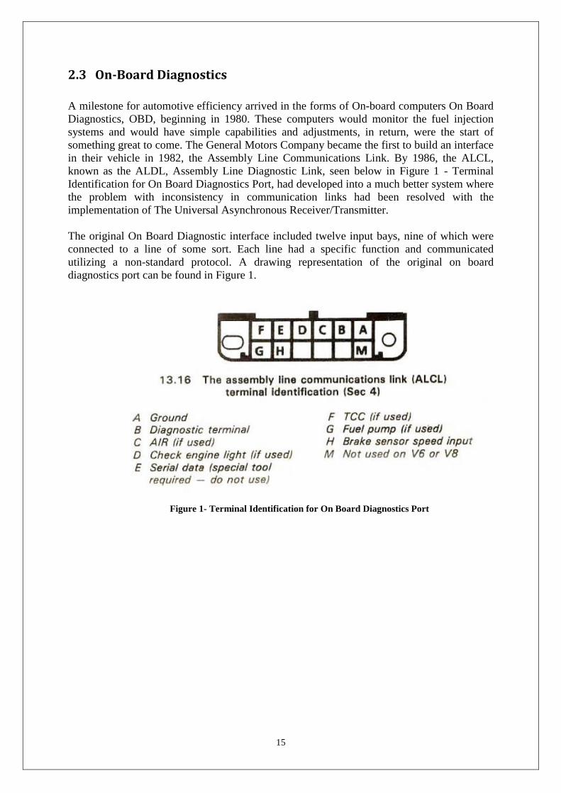
The original On Board Diagnostic interface included twelve input bays, nine of which were
connected to a line of some sort. Each line had a specific function and communicated
utilizing a non-standard protocol. A drawing representation of the original on board
diagnostics port can be found in Figure 1.
Figure 1- Terminal Identification for On Board Diagnostics Port
16
2.4 Standardization of On-Board Diagnostics
Throughout the growth of emission standards and regulations, the state of California was the
backbone for many of the changes that took place. The California Air Resource Board
(CARB) enforced that all new vehicles that would be sold in California in 1988 would have
an On-Board Diagnostic system incorporated. This became known as OBD-I. In an effort to
clean the air, the CARB anticipated that by monitoring the vehicles overall efficiency by
enforcing yearly emissions testing, the public would desire vehicles that would more reliably
pass inspection. Unfortunately, due to the lack of standardization of the emissions tests and
the variety of OBD-I systems from different manufactures, the annual emissions testing was a
long way from where it needed to be to enforce the public’s vehicles to meet any regulations.
In collaboration with the EPA, CARB conducted an OBD-I case study.
2.5 Introduction of OBD-II
California again led the emissions standards into the next era after six years of on board
diagnostics research. The next generation diagnostics interface was called OBD-II. All new
vehicles sold in California after 1996 are required to meet OBD-II specifications and
standards.
OBD-II is a result of the years of research and development by the Society of Automotive
Engineers (SAE), the CARB and the EPA. Incorporating OBDIs positive aspects, these
engineers developed a system that would be standardized throughout the country in an effort
to successfully enforce emissions standards.
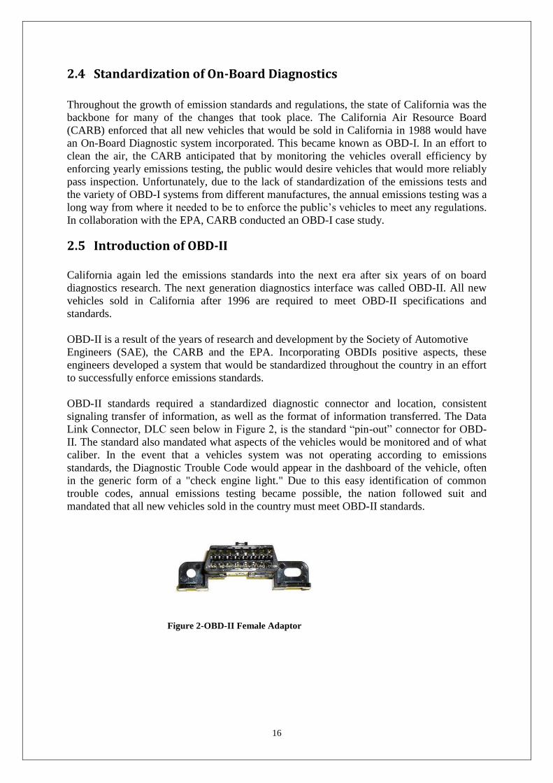
OBD-II standards required a standardized diagnostic connector and location, consistent
signaling transfer of information, as well as the format of information transferred. The Data
Link Connector, DLC seen below in Figure 2, is the standard “pin-out” connector for OBD-
II. The standard also mandated what aspects of the vehicles would be monitored and of what
caliber. In the event that a vehicles system was not operating according to emissions
standards, the Diagnostic Trouble Code would appear in the dashboard of the vehicle, often
in the generic form of a "check engine light." Due to this easy identification of common
trouble codes, annual emissions testing became possible, the nation followed suit and
mandated that all new vehicles sold in the country must meet OBD-II standards.
Figure 2-OBD-II Female Adaptor
17
2.6 Types of OBD-II
There are three types of OBD-II. The first, and oldest standard, is ISO 9141-2. This standard
was defined by the International Organization for Standardization in 1989 in response to the
California Air Resources Board’s call for cleaner emissions.
The second standard was standardized by the Society of Automotive Engineers. The
standardization defined is the SAE J1850 Communications Standard. This standard can be
implemented in one of two ways. The implementation occurs through Variable Pulse Width
(VPW), or Pulse-Width Modulation (PWM).
Recent improvements in automobiles require more computing power distributed around the
vehicle. Due to this increased number of nodes which need to communicate, a newer, faster
bus speed is needed. Further investigation brought CAN, or Controller Area Network, into
focus, and all vehicles sold in the United States after 2008 are required to implement this
standard of communications.
2.6.1 ISO 9141-2
The ISO 9141-2 protocol is based on serial communication using one of two lines. Pin 7 and
Pin 15 are the two lines of communication, and are labeled K line and L line, respectively.
Serial communication transfers bits using high and low voltages to represent bits, 0, or low, is
represented by a zero volt message, 1, or high, is represented by 12 volts.
Communication through ISO 9141-2 is asynchronous and has a data transfer speed of 10.4k
Baud. Data bits have a maximum high to low propagation delay of 2 microseconds.
Similarly, the maximum low to high propagation delay is also 2 microseconds.
This protocol is framed with a certain set of data which includes a header byte, a set of data
bytes, and a checksum byte. The frame is the same as the J1850 messages, and follows the
same message format. The difference lies in the physical architecture.
ISO 9141-2 has a similar protocol to RS-232. The K line is the communication wire, and the
L line is used solely for “waking up” the unit, and is optional and useless other than for this
particular function. The unit can, in fact, be woken up utilizing the K line, which makes the L
line somewhat obsolete.
2.6.1.1 ISO 9141-2 Signaling
The K line of the ISO 9141-2 bus idles high, and is drawn down with messaging. A specific
UART is used in the communication, although not at RS-232 voltage levels. High voltage is
set at the voltage of the battery.
The message frames are signaled to look the exact same as the J1850 protocol, but is
restricted to 12 bytes. There includes a header byte, message body, and an end byte. The ISO
9141-2 standard operates at a frequency of 10,400 bits per second. Because this is a fixed
period, there is no consideration for bit timing. Bits are represented by the line’s state and the

18
line’s state only. When the line is “high,” the bit is equal to 1, when the line is “low,” the bit
is equal to 0. Consecutive bits which are the same cause no edge on the line and the line will
continue at that value.
2.6.1.2 Initiation Protocol
Connecting to an ISO 9141 capable OBD-II port requires a sequence of handshaking steps in
order to communicate. The process is as follows:
1. Select the K line from the OBD-II wiring harness to use as Serial Communications
2. Set outgoing communication to 5 baud
3. Transmit a hex value of 0x33h to the OBD-II Port
4. Immediately set incoming/outgoing communications to 10400 baud
5. The line is now half duplex and the OBD-II Port should echo 0x33h
6. A response from the OBD-II will read 0x55h
Since this was the first standard put into place for OBD-II communication, it is somewhat
limited in its functionality. There is no error checking available to programmers and it is the
slowest type of communication. The communication between the OBD-II scan tool and the
OBD-II port is very structured and cannot be interrupted. Once a command is sent, the sender
must wait for a response from the receiver.
2.6.2 SAE J1850
The SAE J1850 standard was a recommended standard for seven years before being officially
adopted by the Society of Automotive Engineers in February, 1994.4 The standard which has
come to be known as SAE J1850 is a Class B classification. There are two types of pulse
modulation. Frequency Division Multiplexing, which transmits two or more messages
simultaneously on a single channel, and Time division multiplexing, which interleaves two or
more signals on the same channel for either a fixed or a variable length of time.
2.6.2.1 J1850 Implementation Types
There are two implementations of the J1850 standard. The first is Variable-Pulse Width
(VPW) modulation. VPW occurs at 10.4Kbps, and uses a variable time length and division
multiplexing approach to transmit signals.
The second implementation of J1850 involves Pulse-Width Modulation, or PWM. Pulse-
Width Modulation is a method of communication that involves a fixed width pulse. There is a
fixed period square wave form which has a duty cycle. PWM is commonly used in drills to
change drill bit speed, and light dimmers, which give a linear brightness scale to a light
source, allowing the light to have a 0% duty cycle (absolutely dark), or a 100% duty cycle
(bright as designed).
19
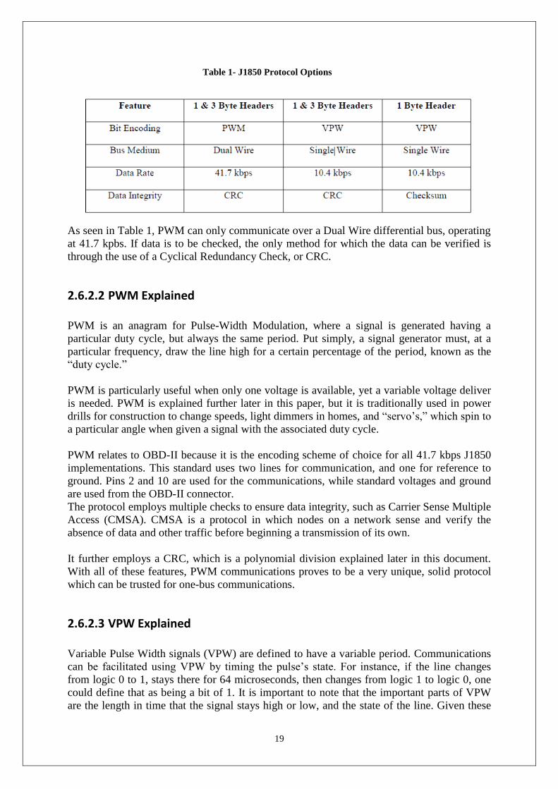
Table 1- J1850 Protocol Options
As seen in Table 1, PWM can only communicate over a Dual Wire differential bus, operating
at 41.7 kpbs. If data is to be checked, the only method for which the data can be verified is
through the use of a Cyclical Redundancy Check, or CRC.
2.6.2.2 PWM Explained
PWM is an anagram for Pulse-Width Modulation, where a signal is generated having a
particular duty cycle, but always the same period. Put simply, a signal generator must, at a
particular frequency, draw the line high for a certain percentage of the period, known as the
“duty cycle.”
PWM is particularly useful when only one voltage is available, yet a variable voltage deliver
is needed. PWM is explained further later in this paper, but it is traditionally used in power
drills for construction to change speeds, light dimmers in homes, and “servo’s,” which spin to
a particular angle when given a signal with the associated duty cycle.
PWM relates to OBD-II because it is the encoding scheme of choice for all 41.7 kbps J1850
implementations. This standard uses two lines for communication, and one for reference to
ground. Pins 2 and 10 are used for the communications, while standard voltages and ground
are used from the OBD-II connector.
The protocol employs multiple checks to ensure data integrity, such as Carrier Sense Multiple
Access (CMSA). CMSA is a protocol in which nodes on a network sense and verify the
absence of data and other traffic before beginning a transmission of its own.
It further employs a CRC, which is a polynomial division explained later in this document.
With all of these features, PWM communications proves to be a very unique, solid protocol
which can be trusted for one-bus communications.
2.6.2.3 VPW Explained
Variable Pulse Width signals (VPW) are defined to have a variable period. Communications
can be facilitated using VPW by timing the pulse’s state. For instance, if the line changes
from logic 0 to 1, stays there for 64 microseconds, then changes from logic 1 to logic 0, one
could define that as being a bit of 1. It is important to note that the important parts of VPW
are the length in time that the signal stays high or low, and the state of the line. Given these
20
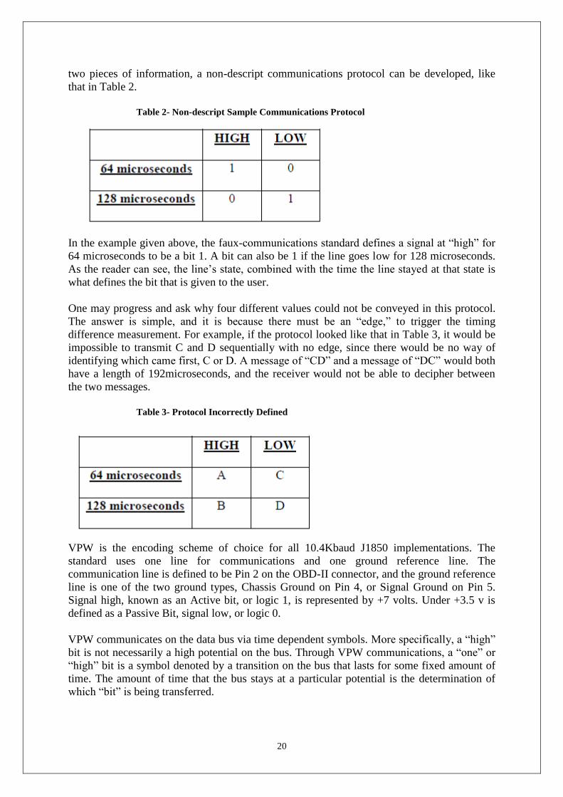
two pieces of information, a non-descript communications protocol can be developed, like
that in Table 2.
Table 2- Non-descript Sample Communications Protocol
In the example given above, the faux-communications standard defines a signal at “high” for
64 microseconds to be a bit 1. A bit can also be 1 if the line goes low for 128 microseconds.
As the reader can see, the line’s state, combined with the time the line stayed at that state is
what defines the bit that is given to the user.
One may progress and ask why four different values could not be conveyed in this protocol.
The answer is simple, and it is because there must be an “edge,” to trigger the timing
difference measurement. For example, if the protocol looked like that in Table 3, it would be
impossible to transmit C and D sequentially with no edge, since there would be no way of
identifying which came first, C or D. A message of “CD” and a message of “DC” would both
have a length of 192microseconds, and the receiver would not be able to decipher between
the two messages.
Table 3- Protocol Incorrectly Defined
VPW is the encoding scheme of choice for all 10.4Kbaud J1850 implementations. The
standard uses one line for communications and one ground reference line. The
communication line is defined to be Pin 2 on the OBD-II connector, and the ground reference
line is one of the two ground types, Chassis Ground on Pin 4, or Signal Ground on Pin 5.
Signal high, known as an Active bit, or logic 1, is represented by +7 volts. Under +3.5 v is
defined as a Passive Bit, signal low, or logic 0.
VPW communicates on the data bus via time dependent symbols. More specifically, a “high”
bit is not necessarily a high potential on the bus. Through VPW communications, a “one” or
“high” bit is a symbol denoted by a transition on the bus that lasts for some fixed amount of
time. The amount of time that the bus stays at a particular potential is the determination of
which “bit” is being transferred.
21
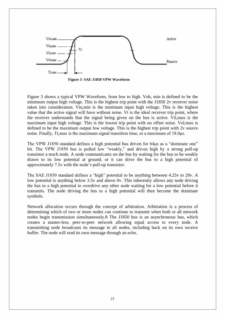
Figure 3- SAE J1850 VPW Waveform
Figure 3 shows a typical VPW Waveform, from low to high. Voh, min is defined to be the
minimum output high voltage. This is the highest trip point with the J1850 2v receiver noise
taken into consideration. Vin,min is the minimum input high voltage. This is the highest
value that the active signal will have without noise. Vt is the ideal receiver trip point, where
the receiver understands that the signal being given on the bus is active. Vil,max is the
maximum input high voltage. This is the lowest trip point with no offset noise. Vol,max is
defined to be the maximum output low voltage. This is the highest trip point with 2v source
noise. Finally, Tt,max is the maximum signal transition time, or a maximum of 18.0μs.
The VPW J1850 standard defines a high potential bus driven for 64μs as a “dominate one”
bit. The VPW J1850 bus is pulled low “weakly,” and driven high by a strong pull-up
transistor a teach node. A node communicates on the bus by waiting for the bus to be weakly
drawn to its low potential at ground, or it can drive the bus to a high potential of
approximately 7.5v with the node’s pull-up transistor.
The SAE J1850 standard defines a “high” potential to be anything between 4.25v to 20v. A
low potential is anything below 3.5v and above 0v. This inherently allows any node driving
the bus to a high potential to overdrive any other node waiting for a low potential before it
transmits. The node driving the bus to a high potential will then become the dominate
symbols.
Network allocation occurs through the concept of arbitration. Arbitration is a process of
determining which of two or more nodes can continue to transmit when both or all network
nodes begin transmission simultaneously.8 The J1850 bus is an asynchronous bus, which
creates a master-less, peer-to-peer network allowing equal access to every node. A
transmitting node broadcasts its message to all nodes, including back on its own receive
buffer. The node will read its own message through an echo.
22
2.6.3 Controller Area Networks
2.6.3.1 CAN Background
Robert Bosch GmbH, the world’s largest automotive components supplier, pursued a method
to better communication within a vehicle’s electrical and mechanical system. Bosch chose the
Intel Corporation, the world’s largest semiconductor company, to join on this venture. The
objective for the electrical and mechanical system project was to make automobiles more
efficient in respect to fuel consumption, emissions, weight, and reliability. Together in 1983,
these companies delivered the Controller Area Network, CAN.
Controller Area Networks is a protocol that uses content addressed messaging in a broadcast
manor. Every node on the network receives every message transmitted. Acknowledgement
immediately is sent and the message is then discarded or kept to be processed by each node.
By using CSMA/CD (Carrier Sense Multiple Access/Collision Detection) each node can gain
access to the bus equally, and by using dominant and recessive identification, the process
runs smoothly with the appropriate information arriving first. Fault Confinement is used by
CAN to address faulty nodes and if need be, automatically turning them off to guarantee the
network’s availability.
2.6.3.2 Message / Frame Types
CAN uses a message based protocol often referred to as ‘content-addressed.’ Content-
addressed implies that each message has the destination within. A priority and the data to be
transferred is embedded into the message and broadcasted to every node on the network. It is
up to the nodes to acknowledge that the message was received properly and to discard or
process the message. Messages can be sent to an abundance of nodes and processed or
processed by a single node according to who is destined to receive it. Messages are referred
to as ‘Frames’ and there are four types of frames in the CAN protocol. The frame types are
defined as the Data Frame, Remote Frame, Error Frame, and Overload Frame. Each type is
explained below in Table 2.
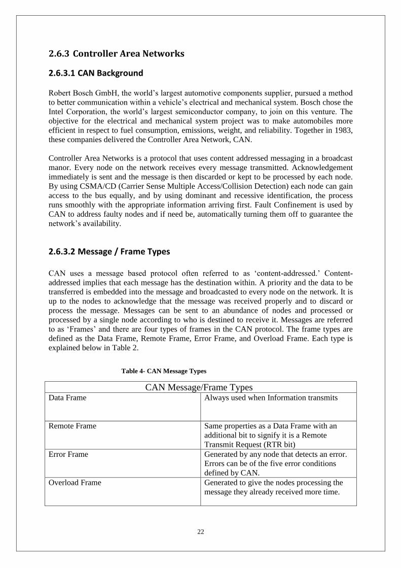
Table 4- CAN Message Types
CAN Message/Frame Types Data Frame Always used when Information transmits
Remote Frame Same properties as a Data Frame with an
additional bit to signify it is a Remote
Transmit Request (RTR bit)
Error Frame Generated by any node that detects an error.
Errors can be of the five error conditions
defined by CAN.
Overload Frame Generated to give the nodes processing the
message they already received more time.

23
2.6.3.3 Speed and Voltages
CAN is defined by ISO 11898 or ISO 114519. Data transfer rates range from a maximum of
1Mbps to a minimum of 10kbps. Communication lines used on the OBDII connector are Pin
6 as a high, Pin14 as a low. In addition CAN uses two ground types, Pin 4 as the Chassis
Ground, and Pin 5 as the Signal Ground. The two communication lines operate in a
differential mode where the voltages carried are inverted to decrease noise interference. Pin
16 is the voltage of the battery. Below in the Table 5 are the standards for the voltage levels
for both the ISO 11898 and ISO 11519;
Table 5- ISO 11519
Signal Recessive State Dominant State Unit
Min Nominal Max Min Nominal Max
CAN-High 1.6 1.75 1.9 3.85 4.0 5.0 Volt
CAN-Low 3.1 3.25 3.4 0 1.0 1.15 Volt
2.6.3.4 Network Structure An example Controller Area Network may be seen below in Figure 4. There are a multitude
of devices such as emissions, safety, control devices, and many others. Each device
communicates with a host processor via a CAN Controller connected to the bus.
Figure 4- CAN Network in Practice
24
2.6.3.5 Node Structure
Nodes are composed of a host processor, a CAN controller, and a transceiver. In a node, the
host processor will derive received messages and will calculate what messages to transmit.
The CAN Controller is the primary means of sending and receiving messages within a node.
To send, once the host processor has completely stored the desired message to be transmitted
into the CAN Controller, transition will commence in the form of bits serially onto the bus.
To receive, the CAN Controller serially stores bits and is available if the message pertains to
the host processors request. A CAN Controller has a synchronous clock. The final part of the
node structure is a Transceiver often built into the CAN Controller. The Transceiver
translates transmitted and received messages to and from the bus and the controller
respectively. While receiving, the Transceiver will adjusts the signal levels from the bus to
those the CAN Controller can process.
While sending, the Transceiver takes converts the signal provided by the CAN Controller to
that of which the bus requires. In addition to the Transceiver’s receiving and sending
capabilities, it also provides the CAN Controller with a buffer protective circuitry layer.
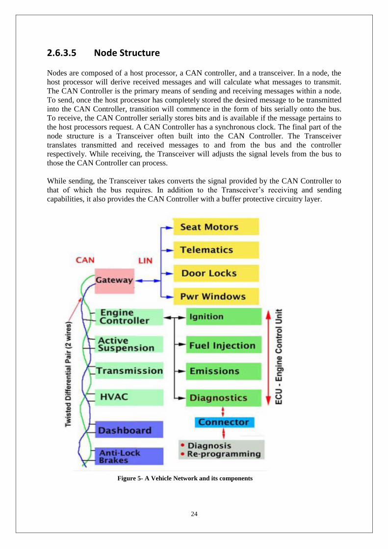
Figure 5- A Vehicle Network and its components
25
Figure 5 connects a Controller Area Network bus with a Local Interconnect Network bus by a
gateway located within one of the Electronic Control Modules of the vehicle most often in
the Engine Control Unit. The Engine Control Unit is where the vital engine control functions
are located and is a clearinghouse for the vehicle’s diagnostics in this case, OBD-II.
2.6.4 OBD-II Modes and Parameter IDs (PIDs)
A parameter ID (PID) is a unique code or command that OBD assigns to a specific data
request type. So in order to communicate with an ECU using OBD-II, you must first send the
appropriate PID for the type of information you want and the ECU will then respond with a
sequence of bytes. The bytes are usually expressed in hexadecimal format. The OBD-II
standard does not require vehicle manufacturers to implement all PIDs. In fact, it doesn’t
even give a minimum for some modes such as Mode 1 and Mode 2 PIDs. However, most
manufacturers implement the most common ones such as vehicle speed and engine RPM.
Since there are different categories of requests, the OBD-II standard breaks the PIDs up into
groups, known as modes. In the original J1979 specification document of the SAE, it listed 9
diagnostic test modes. They are as follows:
Mode 1: PIDs in this category display current real time data such as the results of the
engine RPM sensor.
Mode 2: When a fault or malfunction occurs, a snap shot of all mode 1 sensors are
taken. This snap shot is known as a freeze frame. To access each individual sensor,
you use the mode 2 requests.
Mode 3: Sending a mode 3 request, the ECU responds with a list of DTCs stored if
any.
Mode 4: Sending a mode 4 request, the ECU clears the DTCs stored and turns off the
malfunction indicator lamp (MIL) if on.
Mode 5: Test results from oxygen sensor monitoring
Mode 6: Test results from other types of tests
Mode 7: Show pending Diagnostic Trouble Codes
Mode 8: Control operation of on-board system
Mode 9: Responds with the vehicles identification number (VIN).
Since the original specification, other modes have been added on and a lot are manufacturer
specific. To send a request to the ECU you must specify the mode and the PID. So for
example, if I want to view the current engine RPM, I would send a 010Ch (hexadecimal)
query to the ECU. The ECU would then respond with a few bytes of data for the response. If
I wanted to see the engine RPM stored value when a fault occurred last on the vehicle, I
would instead send a mode 2 query, 020Ch. As you can see the query or command to send to
an ECU is a combination of the mode and the relevant PID. All requests must adhere to this
request format.
26
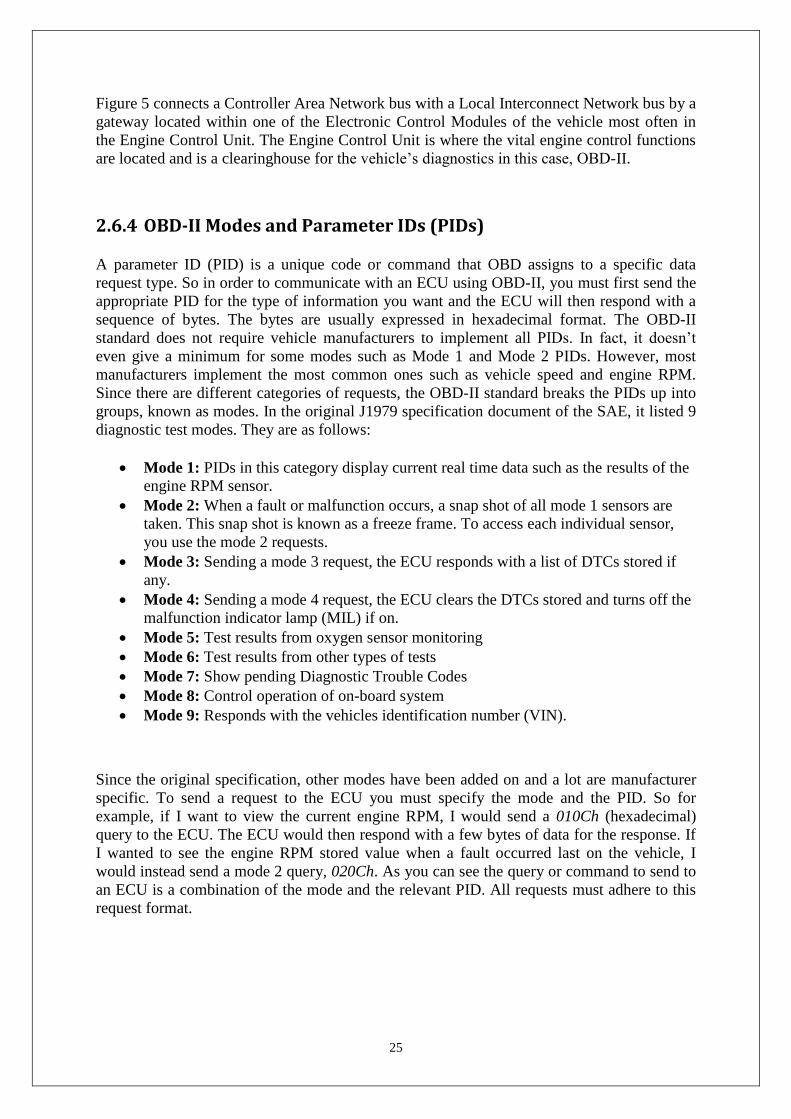
2.6.4.1 How data is sent on the ECU bus
Naturally the data isn’t sent to the ECU bus in raw bytes having just the mode and the PID
thrown on the wire. The message (mode and PID) is encapsulated in a header and footer.
Figure 6 shows the format of a typical OBD-II message. Since OBD-II works on a bus based
technology, the identification of source and destination need to be accounted for. Without it
the scan tool would never be able to locate the message that is destined for it. The header
format includes 3 fields, a priority field, a sender or source address (SA) and a receiver or
target address (TA). OBD-II’s messaging works on a priority based scheme. Some messages
within an engine’s management system are more critical than others. For example,
communication with the ABS system is critical and that should always get priority over
something like a scan tool. Our message such as 010C is placed in the payload section of the
packet. Normally this is just 2 bytes; the mode and the PID but some PIDs require extra data
to be sent after it so 7 bytes in total are allowed. The checksum at the end is to ensure
integrity. It should be noted that this is the normal OBD-II message format. CAN has extra
fields placed in it as it is a more complex protocol capable of transferring a lot more
information at higher speeds. Discussion on this protocol is out of scope for this project.
Figure 6-The format of an OBD-II 2 message
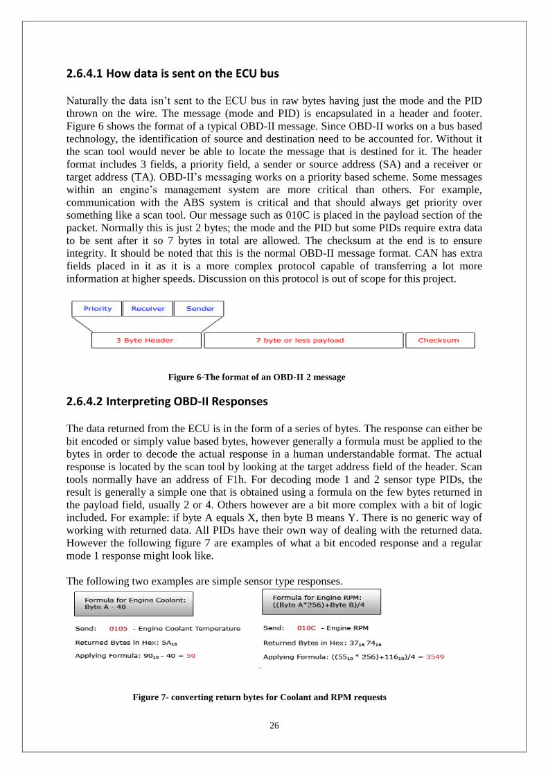
2.6.4.2 Interpreting OBD-II Responses
The data returned from the ECU is in the form of a series of bytes. The response can either be
bit encoded or simply value based bytes, however generally a formula must be applied to the
bytes in order to decode the actual response in a human understandable format. The actual
response is located by the scan tool by looking at the target address field of the header. Scan
tools normally have an address of F1h. For decoding mode 1 and 2 sensor type PIDs, the
result is generally a simple one that is obtained using a formula on the few bytes returned in
the payload field, usually 2 or 4. Others however are a bit more complex with a bit of logic
included. For example: if byte A equals X, then byte B means Y. There is no generic way of
working with returned data. All PIDs have their own way of dealing with the returned data.
However the following figure 7 are examples of what a bit encoded response and a regular
mode 1 response might look like.
The following two examples are simple sensor type responses.
-
Figure 7- converting return bytes for Coolant and RPM requests

27
2.6.4.3 Interpreting Diagnostic Trouble Codes (DTCs) There are four main types of DTC codes defined by the SAE standards. These are the
following: First digit will be:
• Powertrain Codes (P codes) 0 - 3
• Chassis Codes (C codes) 4 - 7
• Body Codes (B codes) 8 - B
• Network Codes (U codes) C - F
These codes identify where or what system the fault occurred. The powertrain codes are the
most common and represent codes that occur in the engine management system. Diagnostic
trouble codes are made up of 5 digits. The digits are in hexadecimal format. The first digit
always identifies the type code whether it a powertrain code, body code etc. In the above list,
you can see the range of digits that identify what category of codes it belongs to. The other 4
digits in the code identify other information. For example the second digit identifies if it is a
standard SAE defined code or a proprietary while the third digit identifies what system
caused the fault. Belowin figure 8 is a diagram that illustrates the format of a code.
Figure 8- example of Diagnostic Trouble Codes
28
3 Proposed Approach
Approach for this project actually had two different paths in two semesters. First semester
approach is completely different than the second semester approach. After the first semester
project evaluation, project approach had to be changed in a proper manner with good
guidance from supervisor. Even though the first semester approach was a failure it gave the
main idea and gave the new goal for the second semester. Following figures shows the
project frame works followed in semester one and two separately.
3.1 First semester approach
3.1.1 Get QT (Quick Time) Applications Executing on Display
This is one of the critical milestones of this project. Without having QT working on the
embedded display, the project would be a major failure. All I will be left with is software that
only runs on a standard desktop or laptop computer which is only part of what is involved
with this project. Before coding starts, this is the mile stone that needs to be achieved first to
prove the concepts used later will work. It is too much of a risk to develop the application
first and then attempt to deploy it later on the display.
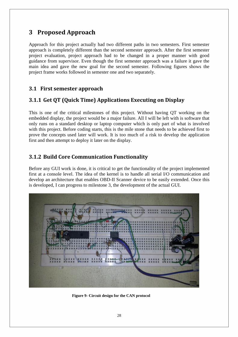
3.1.2 Build Core Communication Functionality
Before any GUI work is done, it is critical to get the functionality of the project implemented
first at a console level. The idea of the kernel is to handle all serial I/O communication and
develop an architecture that enables OBD-II Scanner device to be easily extended. Once this
is developed, I can progress to milestone 3, the development of the actual GUI.
Figure 9- Circuit design for the CAN protocol
29
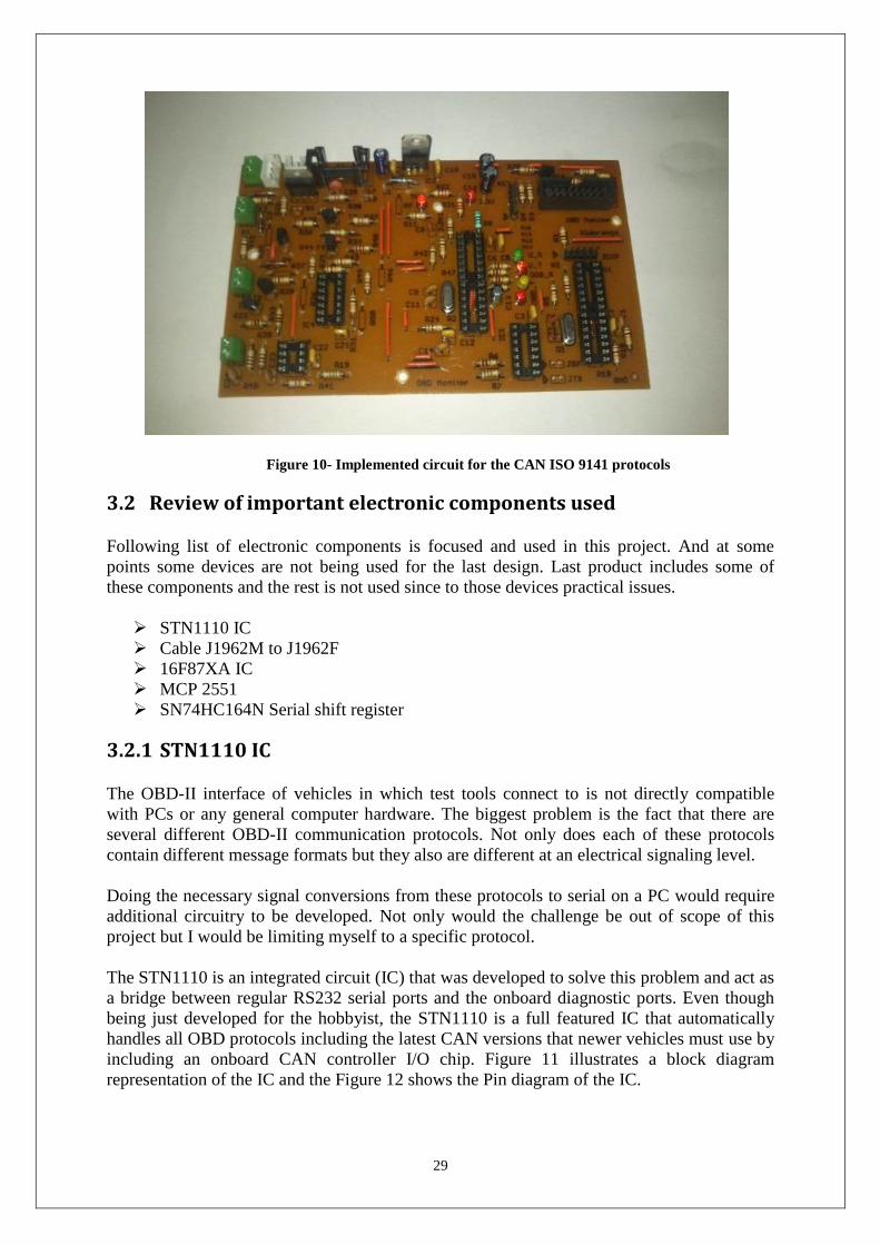
Figure 10- Implemented circuit for the CAN ISO 9141 protocols
3.2 Review of important electronic components used
Following list of electronic components is focused and used in this project. And at some
points some devices are not being used for the last design. Last product includes some of
these components and the rest is not used since to those devices practical issues.
STN1110 IC
Cable J1962M to J1962F
16F87XA IC
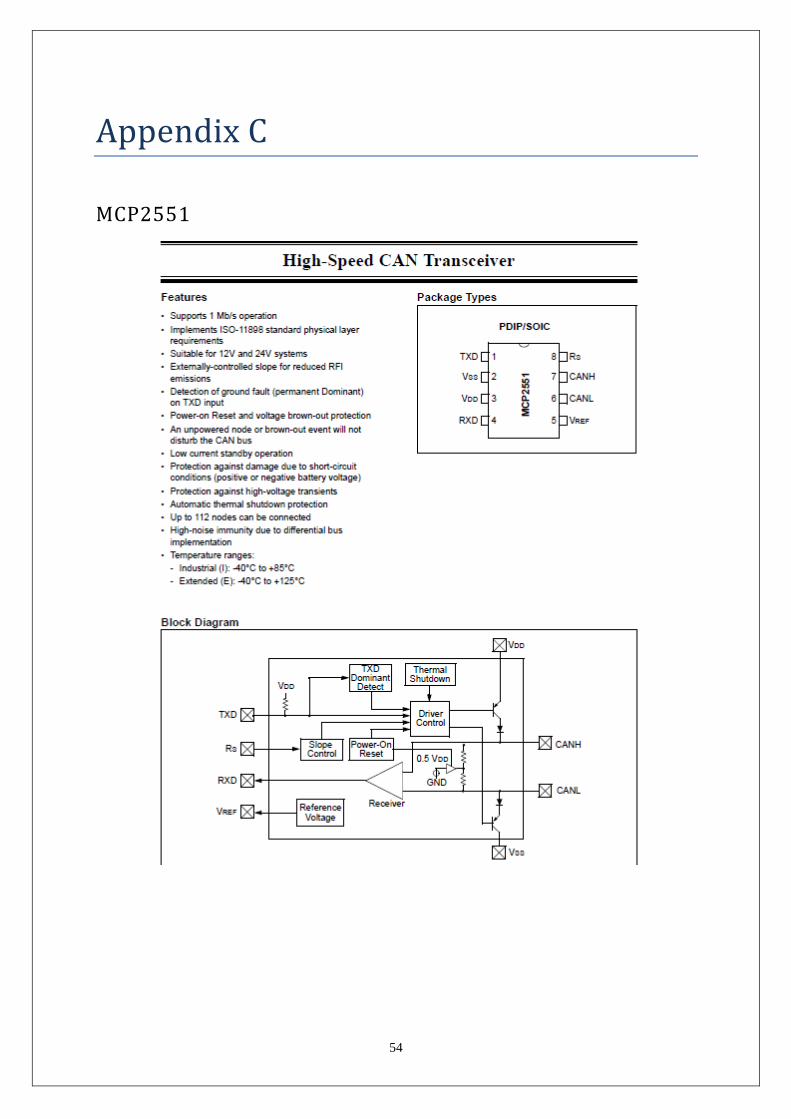
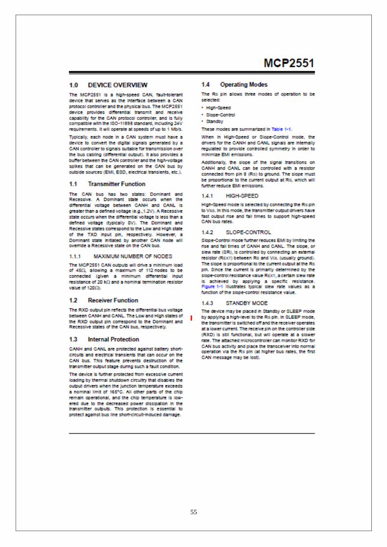
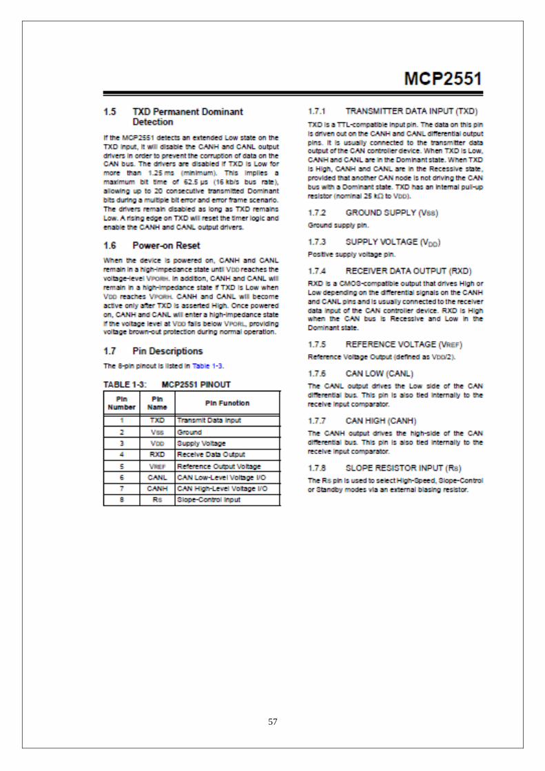
MCP 2551
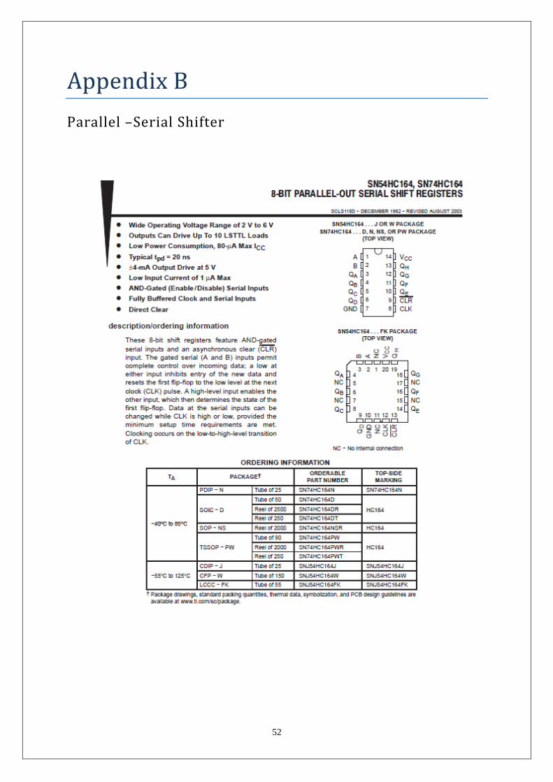
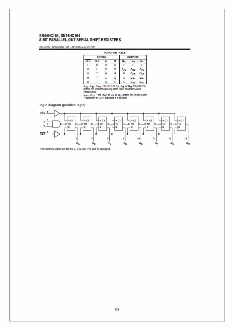
SN74HC164N Serial shift register
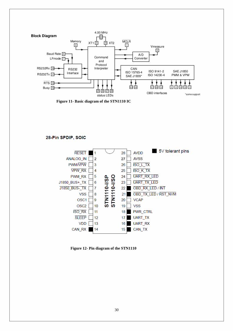
3.2.1 STN1110 IC
The OBD-II interface of vehicles in which test tools connect to is not directly compatible
with PCs or any general computer hardware. The biggest problem is the fact that there are
several different OBD-II communication protocols. Not only does each of these protocols
contain different message formats but they also are different at an electrical signaling level.
Doing the necessary signal conversions from these protocols to serial on a PC would require
additional circuitry to be developed. Not only would the challenge be out of scope of this
project but I would be limiting myself to a specific protocol.
The STN1110 is an integrated circuit (IC) that was developed to solve this problem and act as
a bridge between regular RS232 serial ports and the onboard diagnostic ports. Even though
being just developed for the hobbyist, the STN1110 is a full featured IC that automatically
handles all OBD protocols including the latest CAN versions that newer vehicles must use by
including an onboard CAN controller I/O chip. Figure 11 illustrates a block diagram
representation of the IC and the Figure 12 shows the Pin diagram of the IC.
30
Figure 11- Basic diagram of the STN1110 IC
Figure 12- Pin diagram of the STN1110
31
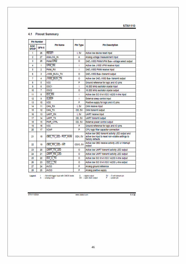
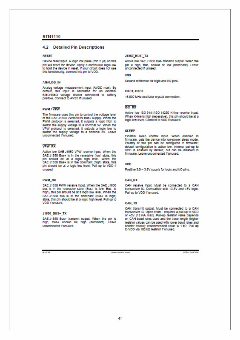
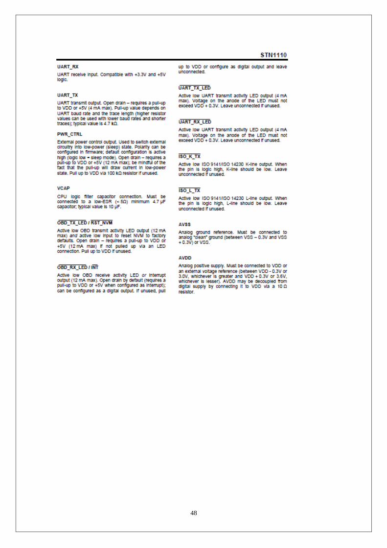
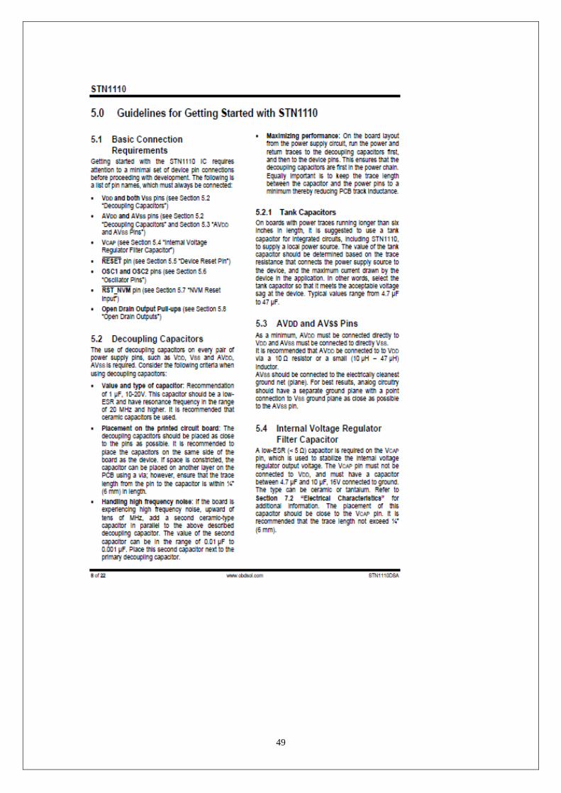
3.2.1.1 Feature Highlights
Microcontroller core features (Refer Appendix A)
There are three types of commands recognized by the STN11xx: AT commands, ST
commands, and OBD requests.
The STN11xx is designed to fully emulate the ELM327 AT command set supported by
many existing OBD software applications. AT commands begin with “AT” and are intended
for the IC. They cause the STN11xx to carry out some action – change or display settings,
perform a reset, and so on. A list of supported AT commands can be found in section 5.0.
In order to provide additional functionality while maintaining compatibility with the ELM327
command set, the STN11xx supports a parallel ST command set, described in section 6.0.
OBD requests are messages that are transmitted on the OBD bus. Only ASCII hexadecimal
digits (0-9 and A-F) are allowed in OBD requests.
• Fully compatible with the ELM327 AT command set
• Extended ST command set
• UART interface (baud rates from 38 bps to 10 Mbps1)
• Secure boot loader for easy firmware updates
• Support for all legislated OBD-II protocols:
ISO 15765-4 (CAN)
ISO 14230-4 (Keyword Protocol 2000)
ISO 9141-2 (Asian, European, Chrysler vehicles)
J1850 VPW (GM vehicles)
J1850 PWM (Ford vehicles)
• Support for non-legislated OBD protocols:
ISO 15765
ISO 11898 (raw CAN)
• Superior automatic protocol detection algorithm
• Large memory buffer
• Voltage input for battery monitoring
Available in TQFP-44 and QFN-44 packages
32
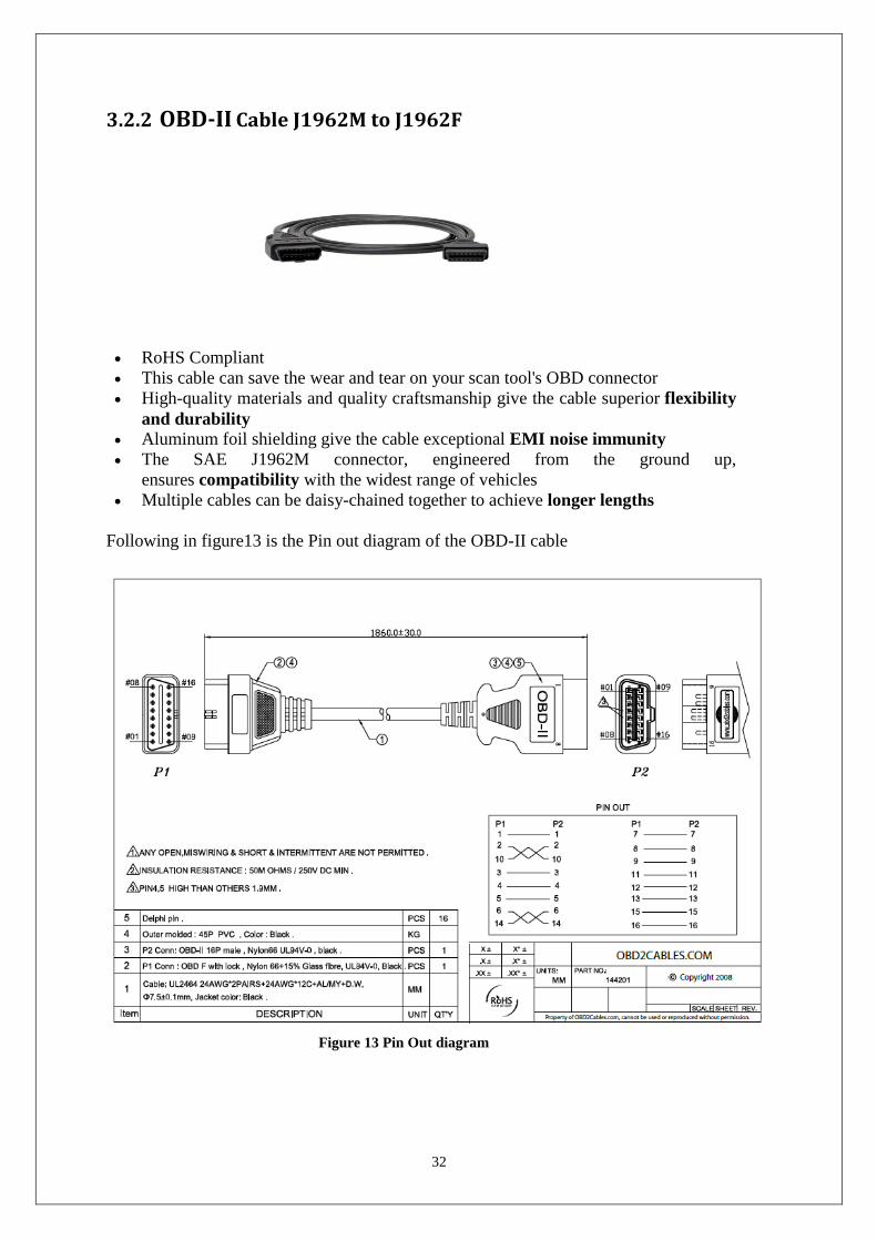
3.2.2 OBD-II Cable J1962M to J1962F
RoHS Compliant
This cable can save the wear and tear on your scan tool's OBD connector
High-quality materials and quality craftsmanship give the cable superior flexibility
and durability Aluminum foil shielding give the cable exceptional EMI noise immunity
The SAE J1962M connector, engineered from the ground up,
ensures compatibility with the widest range of vehicles
Multiple cables can be daisy-chained together to achieve longer lengths
Following in figure13 is the Pin out diagram of the OBD-II cable
Figure 13 Pin Out diagram
33
3.2.3 16F87XA IC
Microcontroller core features (Refer Appendix A)
High performance RISC CPU
Only 35 single word instructions to learn
All single cycle instructions except for program branches which are two cycle
Operating speed: DC - 20 MHz clock input,DC - 200 ns instruction cycle
Up to 8K x 14 words of FLASH Program Memory,
Up to 368 x 8 bytes of Data Memory (RAM)
Up to 256 x 8 bytes of EEPROM Data Memory
Pin out compatible to the PIC16C76
Interrupt capability (up to 14 sources)
Eight level deep hardware stack
Direct, indirect and relative addressing modes
Power-on Reset (POR)
Power-up Timer (PWRT) and Oscillator Start-up Timer (OST)
Watchdog Timer (WDT) with its own on-chip RC oscillator for reliable operation
Programmable code protection
Power saving SLEEP mode
Selectable oscillator options
Low power, high speed CMOS FLASH/EEPROM technology
Fully static design
In-Circuit Serial Programming (ICSP) via two pins
Single 5V In-Circuit Serial Programming capability
In-Circuit Debugging via two pins
Processor read/write access to program memory
Wide operating voltage range: 2.0V to 5.5V
High Sink/Source Current: 25 mA
Commercial, Industrial and Extended temperature ranges
Low-power consumption:
- < 0.6 mA typical @ 3V, 4 MHz
- 20 μA typical @ 3V, 32 kHz
- < 1 μA typical standby current
Microcontroller peripheral features:-
Timer0: 8-bit timer/counter with 8-bit prescaler
Timer1: 16-bit timer/counter with prescaler, can be incremented during SLEEP via
external crystal/clock
Timer2: 8-bit timer/counter with 8-bit period register, prescaler and postscaler
Two Capture, Compare, PWM modules
10-bit multi-channel Analog-to-Digital converter

34
3.3 Second semester Approach
Before starting coding, it was important to break up the project into sub systems in order to
iteratively build the system. OBD-II Scanner can be broken up into many areas.
Serial Communication System and Sensor Monitoring
Diagnostics
GUI and Logic
3.3.1 Serial Communication System and Sensor Monitoring One of the most crucial parts of the OBD2 software is the serial communication system.
Almost all actions that OBD-II executes will involve some serial I/O communication with the
STN1110 chip in order to gather information from the ECU or instruct it to perform a task.
The serial communication is all handled using the HyperTerminal. It can handle both once off
commands to the ECU or be set up in such a way to automatically query several sensors
periodically. The primary base class for commands to the ECU is the Command class. It
constructs objects that contain an OBD-II request.
3.4 Testing
3.4.1 Connecting to the vehicle OBD port
First of all you will need to connect the OBD-II board to the OBD port on your vehicle using
the OBD cable. Depending on the make and model of your car, the port location may vary.
Consult your owner’s manual if you cannot locate the port. The mating end of the cable tends
to be a very tight fit and require a bit of force to get it sitting securely, so it’s usually easier to
start hooking everything together between the car and the cable.
Once you have your headers attached to your board, and you’ve connected to your vehicle
using the OBD cable, you can start communicating with OBD-II scanner over through a
serial port. Figure 14 shows how to connect the device using the OBD-II cable.
Figure 14- Connecting the device using the OBD cable
35
Once you have your serial terminal set up, you will communicate with the OBD-II board by
using AT commands. These commands always start with “AT”. The OBD-II board is case
insensitive, so don’t stress about only using capital letters. After sending “AT”, the next
letters sent to the board will be the commands that should be executed by the board.
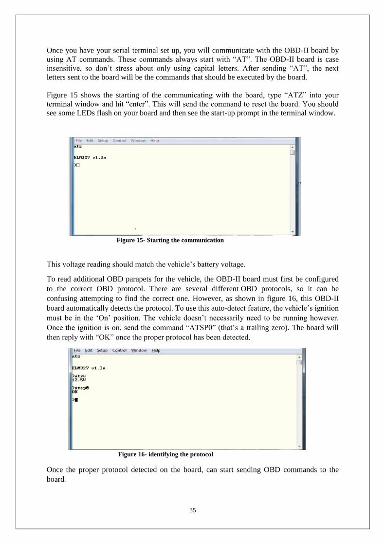
Figure 15 shows the starting of the communicating with the board, type “ATZ” into your
terminal window and hit “enter”. This will send the command to reset the board. You should
see some LEDs flash on your board and then see the start-up prompt in the terminal window.
Figure 15- Starting the communication
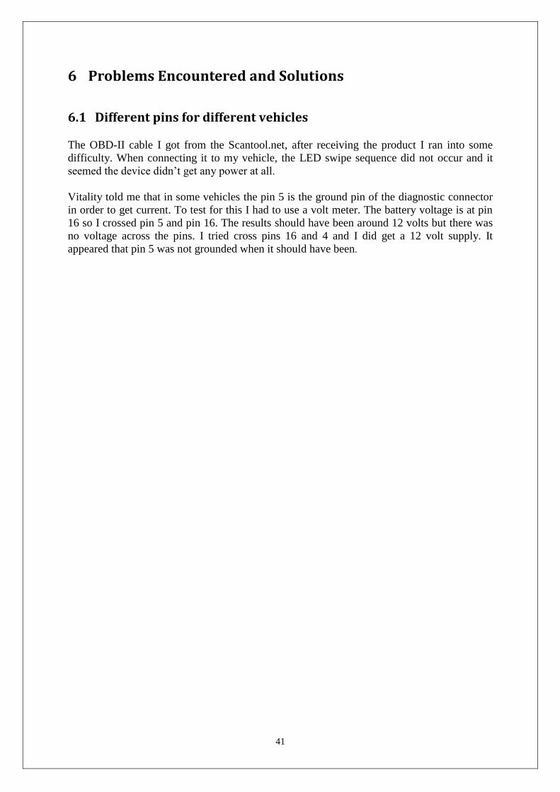
This voltage reading should match the vehicle’s battery voltage.
To read additional OBD parapets for the vehicle, the OBD-II board must first be configured
to the correct OBD protocol. There are several different OBD protocols, so it can be
confusing attempting to find the correct one. However, as shown in figure 16, this OBD-II
board automatically detects the protocol. To use this auto-detect feature, the vehicle’s ignition
must be in the ‘On’ position. The vehicle doesn’t necessarily need to be running however.
Once the ignition is on, send the command “ATSP0” (that’s a trailing zero). The board will
then reply with “OK” once the proper protocol has been detected.
Figure 16- identifying the protocol
Once the proper protocol detected on the board, can start sending OBD commands to the
board.

36
4 Critique
4.1 System Hardware
One of the major design decisions in this lab was to use the STN1110 to communicate with
the vehicle. It is certainly possible, and has been done before, to use a microcontroller to
implement OBD-II communications with a specific brand of car. This is because although the
OBD-II is a standard implemented in all cars sold in the US today, each car company has
implemented it differently as described below, resulting in five distinct signaling protocols.
Because of this, had we chose to implement all of the signaling and modulation in software,
we would only have had time to implement one specific signaling protocol which would only
work on certain types of cars. Because we wanted to be able to interface with many different
types of cars, I chose to use the STN1110.
When deciding on a user interface I knew that I would require user input from buttons as was
implemented in our final design. I also wanted to use an HD 44780 compliant LCD like the
ones used in lab. Since we wanted to display more information and make it easily readable in
a dark car, I chose 16*4 LCD display.
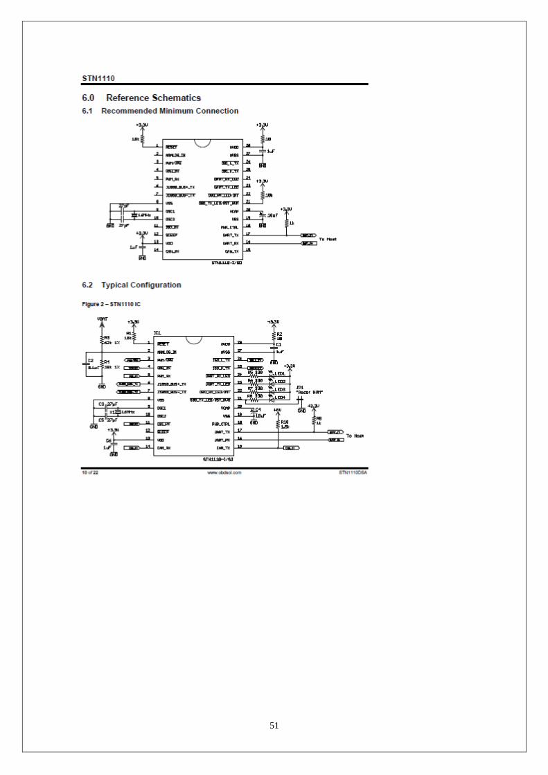
The STN1110 is just an IC and it on its own is not enough. In order to interface with the
STN1110, a circuit needs to be developed. From the block diagram in figure 11 above, it can
be seen that the STN1110 requires a clock or oscillator to power it. ELM Electronics, the
developers of the IC do provide a schematic of a recommended circuit for the ELM327 to fit
in to. This circuit is shown in figure 17.
Figure 17- A recommended circuit for the STN1110

37
4.1.1 Connecting to the IC
The most straight forward way to communicate with the STN1110 is to use a terminal
emulator such as hyper terminal. This allows easy sending of commands to the IC while
receiving the responses in text. This is useful for debugging or getting an idea of what is
available. However, this alone is not very useful. The data returned by the ECU via the
STN1110 is represented in hexadecimal format. The normal user would not benefit from this.
Scanner looks after this low level communication automatically providing a highly user
friendly GUI interface so that users can view real time data or diagnostic trouble codes for
diagnosing problems.
As with all serial communication, certain parameters must be set in order for communication
to occur. The newer versions of the STN1110 include support for high baud rates such as
38400 but this generally will not improve how fast data can be obtained from the ECU as the
OBD-II protocol is a limiting factor.
4.1.2 Communication with the ECU using STN1110
In order to communicate with the ECU, you need to use OBD-II commands as discussed in
the OBD section above. If a command sent to the STN1110 does not begin with the letters
‘A’ and ‘T’ (not case sensitive), then it will assume that the command is an OBD-II one that
is destined for the ECU. It will however, do validation testing to ensure that the command
makes sense.
As discussed previously, OBD-II is a messaging protocol that requires a header and footer to
be added to the command. The STN1110 conveniently looks after the data encapsulation
automatically by adding the necessary physical addresses and generating a checksum for the
FCS field in the footer.
To send an OBD-II command to the ECU, you simply send the ASCII equivalent to the mode
number concatenated with the parameter id (PID). For example, in order to view the current
engine coolant temperature, a mode 01 and PID 0C is required. To send this to the ECU in
order to receive a response, you simply send the ASCII string ‘0105’ to the STN1110. The
STN1110 will then encapsulate this data in the payload field of an OBD-II message and send
it on the ECU’s communication bus. When the ECU is ready, in that it has looked after high
priority messages on the bus, it places a series of bytes on the interface representing its OBD-
II response message that again includes the necessary header and footer. The ELM327 will
wait until it locates the message, identifying it by the destination or target address (TA) in the
header field. It will then do a checksum and if correct, extract the payload bytes and send it
back to the serial port in the form of ASCII characters that represent the hexadecimal data
followed by a ‘>’ prompt character to signify the end of the message.
When the STN1110 places the OBD-II command on the ECU bus, it waits a fixed time for
the message (even if the ECU sent all data) in case more is to follow. If no data is returned,
the STN1110 will send a “NO DATA” message back to the terminal connected to it. A “NO
DATA” could result in an OBD-II PID request that is not supported by the ECU. This is quite
common as different ECU’s support different PIDs. However, if the ECU does reply, the
STN1110 stays waiting in case it receives more bytes from the ECU.

38
Figure 18-ISO Transceiver
Figure 18 shows the sketch diagram of the ISO Transceiver designed and Figure 19 shows
the schematic diagram of the CAN Transceiver while the Figure 20 shows the combined
circuit diagrams of both CAN and ISO Transceivers with the power circuit.
Figure 19-CAN Transceiver
Figure 20- Final circuit

39
4.2 System Software System software is designed by microcontroller programming. Timers and interrupt
peripherals are used in the program. Program flow is developed according to the project
framework mentioned in the above.
The software for the OBD-II Scanner makes use of a state machine to drive the UART
communication based upon a given menu state. The software design begins with an upper
level state machine, describing the interaction between the menu architecture and the UART
communication. Following the chart are descriptions of the menu architecture and device
functionality, UART communication, macros, and button dynamics.
4.2.1 GUI and Logic
This scanner separates the GUI from the main low level serial I/O and ECU communication
components. It does this by creating a package or a name space in which all these low level
components and classes exist. The GUI is not part of this package and it communicates with
the STN1110 interface in order to perform all low level tasks such as loading DTCs, sending
serial I/O commands etc.
The GUI is developed on top of this kernel and implements the main logic for the application.
For example, the acceleration test uses sensor monitoring in the kernel but the higher level
logic such as starting counters and stopping monitoring when a speed is reached is all
handled by the GUI.
Figure 21-Upper level state machine

40
5 Costing
Following Table 6 shows the costing of this project. This costing table is not 100% accurate,
because some of the components in the circuit which are used don’t have cost details. But
final total is approximately around 20000 Sri Lankan rupees.
Table 6- Total Cost
Component Shop Quantity Unit Cost
(Rupees)
Cost
(Rupees)
STN1110 Scantool.net 1 4000 4000
OBD-II Cable Scantool.net 1 2000 2000
PIC16F87XA Unitech 1 400 400
MCP2551 1 400 400
Solder boards 2 600 600
12V to 5V regulator 1 450 450
Display 1 1000 1000
UART serial converter 1 700 700
USB extension cable 1 1000 1000
Keypad 1 250 250
Switch 1 50 50
Jumper Wires 250 250
LED 5 50 50
Resistors 300 300
Capacitors 400 400
PIC kit tool 1 2000 2000
Soldering cost 3000 3000
Total Cost 17100
41
6 Problems Encountered and Solutions
6.1 Different pins for different vehicles
The OBD-II cable I got from the Scantool.net, after receiving the product I ran into some
difficulty. When connecting it to my vehicle, the LED swipe sequence did not occur and it
seemed the device didn’t get any power at all.
Vitality told me that in some vehicles the pin 5 is the ground pin of the diagnostic connector
in order to get current. To test for this I had to use a volt meter. The battery voltage is at pin
16 so I crossed pin 5 and pin 16. The results should have been around 12 volts but there was
no voltage across the pins. I tried cross pins 16 and 4 and I did get a 12 volt supply. It
appeared that pin 5 was not grounded when it should have been.
42
7 Future Enhancements
This final section of the report outlines some features that could potentially be implemented
in future releases. The current set of features implement is a minimum to what a consumer
would expect.
7.1 Freeze frame Support
When a fault is detected in the engine management system by the ECU, diagnostic trouble
codes (DTCs) are logged and a copy of the state of all sensors is taken and stored in the form
of a freeze frame. Freeze frame data is essentially just a snap shot of all available sensors.
This recorded state of the engine management system when a fault occurred can be very
useful to mechanics on identifying the root cause of the fault. OBD-II Scanner currently fails
to support this invaluable feature of onboard diagnostics. Implementing such functionality as
this is very feasible. It is only a matter of doing a query of all sensors using mode 2 requests
rather than mode 1. However one problem may be the lack of screen real estate space. The
GUI system would have to be modified in order to accommodate such information. This
could be simply just a matter of creating a new screen and linking to it from the diagnostics
screen using a push button similar to how the rule editor is launched in the monitoring screen.
7.2 Data Logging
Data logging was one of the original requirements of this project but due to the re-scope it
could not be implemented. In the context of this project, data logging could be a background
process that runs during sensor monitoring sessions in this scanner. Data could be written in
real time to a file so the history of values can be retrieved. This would also allow graphical
representations to be shown. This could be very useful in say the likes of an acceleration test.
Time and vehicle speed could be mapped so the curve of where the vehicle accelerates most
rapidly can be seen.

43
8 Conclusion
Due to the intense work done to interface with a vehicle’s diagnostic’s port, I was able to
achieve multiple goals set forth in the initial planning stages of this project. I was able to
successfully interface with a vehicle’s OBD-II port, and send those codes to a computer.
Then I was able to further achieve the goal of sending codes back through the connection to
have those codes delivered to the vehicle’s OBD-II port. The scanner was also able to receive
live codes from the vehicle as those codes change and update as the vehicle is being driven.
This OBD-II Scanner able to successfully interface with a vehicle’s OBD-II port. This OBD-
II port is based on standards that are proprietary and standard across the world. This project
has the ability to interface with a vehicle through J1850 VPW, J1850 PWM, CAN, ISO 9141,
KWM, and variations of these protocols, as well. The ability to do this was paramount in the
creation of this project, and identified the first major milestone in the project.
Overall I am proud of what I have produced. Before I began this project I hadn’t much
experience with PIC programming. I had almost no experience with automation sytems was
also something new to me so overall I’ve gained a huge set of skills in areas in which I think
will be essential tome further down the line.
I could not implement the full set of requirements that were set out before commencement of
this project. However I have implemented at least the minimum. The original requirements
list was not possible to accomplish so a rescore was necessary. Creating the project blog has
been a great benefit to me. It allowed me to express to the public domain what I’ve learned
and the steps that I took in order to reach this point.
However I have made lots of mistakes, lots of failures during this project, I believe that I
learned a great deal not only about automotive standard protocols, but interfaces in general.
Future projects involving the ground-up creation of electronics will run more smoothly due to
the guidance provided by Dr.Lasantha Seneviratne. I would like to officially thank him for all
of his help and guidance throughout the project.
44
9 Reference
Powers, Chuck. 1992. AN1212. [Online] 1992. [Cited: June 23, 2008.]
Valentine, Richard. 1998. Motor Control Electronic Handbook. Motor Control Electronic
Handbook. s.l. : McGraw Hill, 1998.
Mictronics Forum. 2005. AVR J1850 VPW
Stern, Trampas. 2005 AVR J1850 Interface
Diagnostics, OBD. 2005. OBDII Message Structure
Technologies, Werner. 2002. OBD2 Standards/Terms.
Oliver, D John. Implementing the J1850 VPW protocol
Robert Bosch GmbH, CA_ Specifications. 1991
Texas Instruments, Introduction to CA_. 1997.

45
Appendices
Appendix A
STN1110
46
47
48
49
50
51
52
Appendix B
Parallel –Serial Shifter
53
54
Appendix C
MCP2551
55

56
57
58
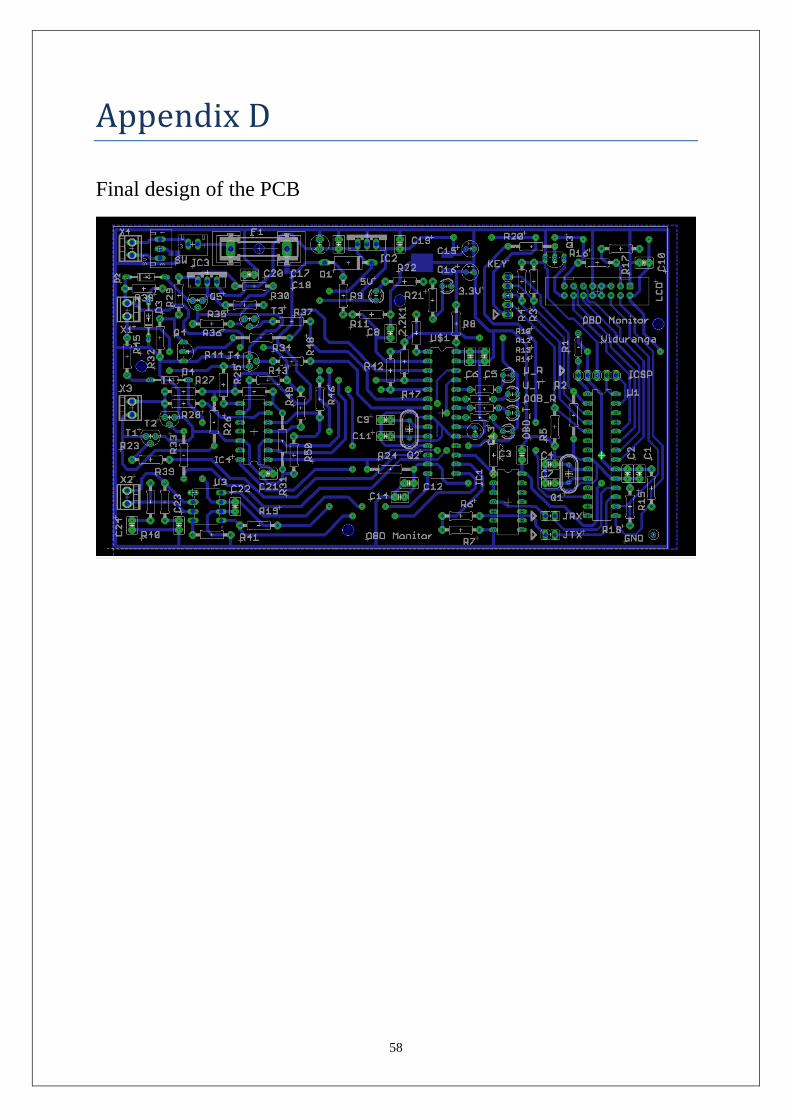
Appendix D
Final design of the PCB


