
ORIGINAL PAPER
Numerical simulation of the impact of polymer rheologyon polymer injectivity using a multilevel local grid refinementmethod
Hai-Shan Luo1 • Mojdeh Delshad1 • Zhi-Tao Li1 • Amir Shahmoradi1
Received: 5 February 2015 / Published online: 10 December 2015
� The Author(s) 2015. This article is published with open access at Springerlink.com
Abstract Polymer injectivity is an important factor for
evaluating the project economics of chemical flood, which
is highly related to the polymer viscosity. Because the flow
rate varies rapidly near injectors and significantly changes
the polymer viscosity due to the non-Newtonian rheologi-
cal behavior, the polymer viscosity near the wellbore is
difficult to estimate accurately with the practical gridblock
size in reservoir simulation. To reduce the impact of
polymer rheology upon chemical EOR simulations, we
used an efficient multilevel local grid refinement (LGR)
method that provides a higher resolution of the flows in the
near-wellbore region. An efficient numerical scheme was
proposed to accurately solve the pressure equation and
concentration equations on the multilevel grid for both
homogeneous and heterogeneous reservoir cases. The
block list and connections of the multilevel grid are gen-
erated via an efficient and extensible algorithm. Field case
simulation results indicate that the proposed LGR is con-
sistent with the analytical injectivity model and achieves
the closest results to the full grid refinement, which con-
siderably improves the accuracy of solutions compared
with the original grid. In addition, the method was vali-
dated by comparing it with the LGR module of
CMG_STARS. Besides polymer injectivity calculations,
the LGR method is applicable for other problems in need of
near-wellbore treatment, such as fractures near wells.
Keywords Polymer rheology � Polymer injectivity �Chemical EOR � Local grid refinement � Non-Newtonianflow
1 Introduction
Polymer flooding has become one of the most widely used
enhanced oil recovery (EOR) methods because of its
adaptability to a wide range of oil viscosity (Wassmuth
et al. 2007), relative simplicity for operations (Mohammadi
and Jerauld 2012), and offshore applicability (Morel et al.
2012). For polymer flooding as well as most other chemical
flooding processes such as surfactant-polymer flood, alka-
line-surfactant-polymer flood, and alkaline-cosolvent-
polymer flood, the polymer injectivity is a key index for
reservoir management, e.g., deciding the upper limit of the
polymer injection rate to optimize the project economics
(Seright et al. 2009). Factors affecting polymer injectivity
include polymer degradation (Seright et al. 2009; Zaitoun
et al. 2012), induced fractures near the injector (Seright
et al. 2009; van den Hoek et al. 2012), polymer
crosslinking to form gel (Bekbauov et al. 2013; Goudarzi
et al. 2013b), and especially polymer rheology (Delshad
et al. 2008; Sharma et al. 2011; Kulawardana et al. 2012).
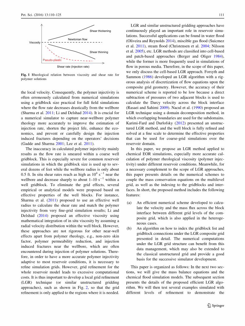
A polymer solution is a non-Newtonian fluid whose vis-
cosity is non-linearly related to the flow rate or the in situ
shear rate. For example, hydrolyzed polyacrylamide
(HPAM) solutions exhibit pseudoplastic behavior at low
shear rates and dilatant behavior at high shear rates when
flowing through porous media as shown in Fig. 1 (Delshad
et al. 2008). In addition, polymer rheology exhibits New-
tonian behavior when the flow is at very low or high rates
(Stahl and Schulz 1988; Sorbie 1991). This behavior leads
to a complex relationship between the pressure drop and
& Hai-Shan Luo
1 Center for Petroleum and Geosystems Engineering, The
University of Texas at Austin, 200 E Dean Keeton St C0300,
Austin, TX 78712, USA
Edited by Yan-Hua Sun
123
Pet. Sci. (2016) 13:110–125
DOI 10.1007/s12182-015-0066-1
the local velocity. Consequently, the polymer injectivity is
often erroneously calculated from numerical simulations
using a gridblock size practical for full field simulations
where the flow rate decreases drastically from the wellbore
(Sharma et al. 2011; Li and Delshad 2014). It is crucial for
a numerical simulator to capture near-wellbore polymer
rheology more accurately to improve the estimation of
injection rate, shorten the project life, enhance the eco-
nomics, and prevent or carefully design the injection
induced fractures depending on the operators’ decisions
(Gadde and Sharma 2001; Lee et al. 2011).
The inaccuracy in calculated polymer injectivity mainly
results as the flow rate is smeared within a coarse well
gridblock. This is especially severe for common reservoir
simulations in which the gridblock size is used up to sev-
eral dozens of feet while the wellbore radius is only about
0.5 ft. In situ shear rates reach as high as 104 s-1 near the
wellbore and decrease sharply to about 1–10 s-1 within a
well gridblock. To eliminate the grid effects, several
empirical or analytical models were proposed based on
effective properties of the well blocks. For instance,
Sharma et al. (2011) proposed to use an effective well
radius to calculate the shear rate and match the polymer
injectivity from very fine-grid simulation results; Li and
Delshad (2014) proposed an effective viscosity using
mathematical integration of in situ viscosity by assuming a
radial velocity distribution within the well block. However,
these approaches are not rigorous for other near-well
effects apart from polymer rheology, e.g., non-zero skin
factor, polymer permeability reduction, and injection
induced fractures near the wellbore, which are often
encountered during injection of polymer solutions. There-
fore, in order to have a more accurate polymer injectivity
adaptive to most reservoir conditions, it is necessary to
refine simulation grids. However, grid refinement for the
whole reservoir model leads to excessive computational
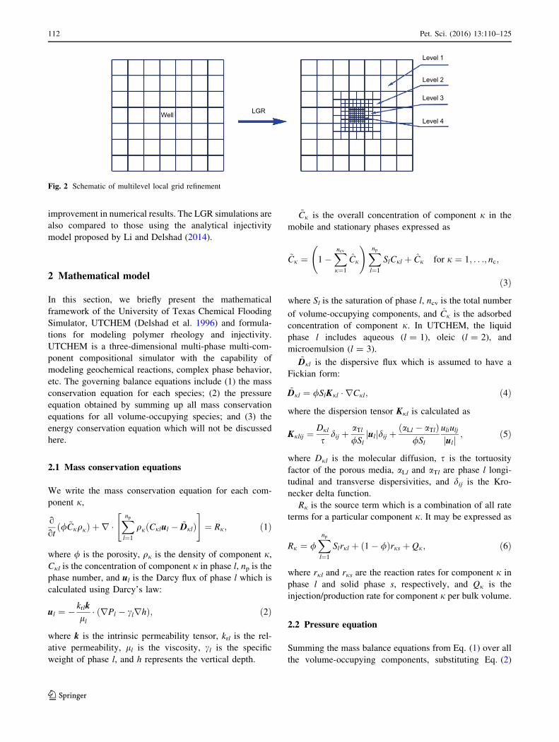
costs. It is thus important to develop a local grid refinement
(LGR) technique (or similar unstructured gridding
approaches), such as shown in Fig. 2, so that the grid
refinement is only applied to the regions where it is needed.
LGR and similar unstructured gridding approaches have
continuously played an important role in reservoir simu-
lations. Successful applications can be found in water flood
(Oliveira and Reynolds 2014), miscible gas flood (Suicmez
et al. 2011), steam flood (Christensen et al. 2004; Nilsson
et al. 2005), etc. LGR methods are classified into cell-based
and patch-based approaches (Berger and Oliger 1984),
while the former is more frequently used in simulations of
flow in porous media. Therefore, in the scope of this paper,
we only discuss the cell-based LGR approach. Forsyth and
Sammon (1986) developed an LGR algorithm with a rig-
orous analysis of discretization of flow equations upon the
composite grid geometry. However, the accuracy of their
numerical scheme is reported to be low because a direct
subtraction of pressures of two adjacent blocks is used to
calculate the Darcy velocity across the block interface
(Rasaei and Sahimi 2009). Nacul et al. (1990) proposed an
LGR technique using a domain decomposition method, in
which overlapping boundaries are used for the subdomains.
Karimi-Fard and Durlofsky (2012) presented an unstruc-
tured LGR method, and the well block is fully refined and
solved at a fine scale to determine the effective properties
that can be used for coarse-grid simulations over the
reservoir domain.
In this paper, we propose an LGR method applied to
chemical EOR simulations, especially more accurate cal-
culation of polymer rheological viscosity (polymer injec-
tivity) under different reservoir conditions. Meanwhile, for
a necessary complement to the scope of LGR approaches,
this paper presents details on the numerical schemes to
couple the mass conservation equations on the multilevel
grid, as well as the indexing to the gridblocks and inter-
faces. In short, the proposed method includes the following
features:
(a) An efficient numerical scheme developed to calcu-
late the velocity and the mass flux across the block
interface between different grid levels of the com-
posite grid, which is also applied in the heteroge-
neous cases.
(b) An algorithm on how to index the gridblock list and
gridblock connections under the LGR composite grid
presented in detail. The numerical computations
under the LGR grid structure can benefit from this
data management, which may also be extended to
the classical unstructured grid and provide a good
basis for the successive simulator development.
This paper is organized as follows: In the next two sec-
tions, we will give the mass balance equations and the
chemical flood simulation models. The subsequent section
presents the details of the proposed efficient LGR algo-
rithm. We will then test several examples simulated with
different levels of refinement to demonstrate the
Shear thickening
Newtonian flow
Shear thinning
Pseudo-plastic
Shear rate (Injection rate)
Viscosity
Fig. 1 Rheological relation between viscosity and shear rate for
polymer solutions
Pet. Sci. (2016) 13:110–125 111
123
improvement in numerical results. The LGR simulations are
also compared to those using the analytical injectivity
model proposed by Li and Delshad (2014).
2 Mathematical model
In this section, we briefly present the mathematical
framework of the University of Texas Chemical Flooding
Simulator, UTCHEM (Delshad et al. 1996) and formula-
tions for modeling polymer rheology and injectivity.
UTCHEM is a three-dimensional multi-phase multi-com-
ponent compositional simulator with the capability of
modeling geochemical reactions, complex phase behavior,
etc. The governing balance equations include (1) the mass
conservation equation for each species; (2) the pressure
equation obtained by summing up all mass conservation
equations for all volume-occupying species; and (3) the
energy conservation equation which will not be discussed
here.
2.1 Mass conservation equations
We write the mass conservation equation for each com-
ponent j,
o
otð/ ~CjqjÞ þ r �
Xnp
l¼1
qjðCjlul � ~DjlÞ" #
¼ Rj; ð1Þ
where / is the porosity, qj is the density of component j,Cjl is the concentration of component j in phase l, np is the
phase number, and ul is the Darcy flux of phase l which is
calculated using Darcy’s law:
ul ¼ � krlk
ll� ðrPl � clrhÞ; ð2Þ
where k is the intrinsic permeability tensor, krl is the rel-
ative permeability, ll is the viscosity, cl is the specific
weight of phase l, and h represents the vertical depth.
~Cj is the overall concentration of component j in the
mobile and stationary phases expressed as
~Cj ¼ 1�Xncv
j¼1
Cj
!Xnp
l¼1
SlCjl þ Cj for j ¼ 1; . . .; nc;
ð3Þ
where Sl is the saturation of phase l, ncv is the total number
of volume-occupying components, and Cj is the adsorbed
concentration of component j. In UTCHEM, the liquid
phase l includes aqueous (l = 1), oleic (l = 2), and
microemulsion (l = 3).~Djl is the dispersive flux which is assumed to have a
Fickian form:
~Djl ¼ /SlKjl � rCjl; ð4Þ
where the dispersion tensor Kjl is calculated as
Kjlij ¼Djl
sdij þ
aTl/Sl
ulj jdij þaLl � aTlð Þ
/Sl
uliulj
ulj j ; ð5Þ
where Djl is the molecular diffusion, s is the tortuosity
factor of the porous media, aLl and aTl are phase l longi-
tudinal and transverse dispersivities, and dij is the Kro-
necker delta function.
Rj is the source term which is a combination of all rate
terms for a particular component j. It may be expressed as
Rj ¼ /Xnp
l¼1
Slrjl þ ð1� /Þrjs þ Qj; ð6Þ
where rjl and rjs are the reaction rates for component j in
phase l and solid phase s, respectively, and Qj is the
injection/production rate for component j per bulk volume.
2.2 Pressure equation
Summing the mass balance equations from Eq. (1) over all
the volume-occupying components, substituting Eq. (2)
Well LGR
Level 1
Level 2
Level 3
Level 4
Fig. 2 Schematic of multilevel local grid refinement
112 Pet. Sci. (2016) 13:110–125
123

and using aqueous phase pressure as a reference pressure,
we obtain the pressure equation:
where Pcl1 is the capillary pressure between phase l and
phase 1 (the aqueous phase), and krlc is the relative
mobility expressed as
krlc ¼krl
ll
Xncv
l¼1
qjCjl; ð8Þ
and Ct represents the total compressibility which is the
volume-weighted sum of the rock matrix (Cr) and com-
ponent compressibilities (Cj0):
Ct ¼ Cr þXncv
l¼1
C0j~Cj; ð9Þ
where / ¼ /R 1þ Cr PR � PR0ð Þ½ �; PR and PR0 are rock
and reference rock pressures.
2.3 Rheological viscosity of the polymer solution
Non-Newtonian polymer rheology (shear-thinning behav-
ior) is modeled using Meter’s equation (Meter and Bird
1964):
lapp ¼ l1 þl0p � l1
1þ _ceff_c1=2
� �Pa�1; ð10Þ
where lapp is the apparent viscosity of the polymer solution;
l1 is the polymer solution viscosity at infinite shear rate
which is assumed to be brine viscosity; _c1=2 is the shear rate at
which the apparent viscosity is the average of l1 and l0p; Pa
is a fitting parameter. For the synthetic polymer, e.g., HPAM,
polymer solutions show shear-thinning behavior at inter-
mediate shear rates and shear-thickening (dilatant) behavior
at high rates. To remediate the deficiency of Meter’s equa-
tion, Delshad et al. (2008) developed a comprehensive
polymer viscosity model which covers the whole shear-rate
regime. The apparent viscosity consists of two parts:
lapp ¼ lsh þ lel; ð11Þ
where the shear-thinning model uses the Carreau model
(Carreau 1968):
lsh ¼ l1 þ l0p � l1� �
1þ k1 _ceffð Þ2h i n1�1ð Þ=2
; ð12Þ
and the shear-thickening model is
lel ¼ lmax 1� exp � k2s _ceffð Þn2�1h in o
; ð13Þ
where a1, a2, and s are all fitting model parameters
obtained by matching experimental data; lmax is given as
lmax ¼ lb AP11 þ AP22lnCp
� �CSpSEP; ð14Þ
where CSpSEP is the polymer viscosity dependence on salinity
and hardness; AP11 and AP22 are fitting parameters. When
AP11 and AP22 are zero, the comprehensive polymer vis-
cosity model reduces to the Carreau model.
The effective shear rate ( _ceff) correlates viscosity mea-
sured in a viscometer to an apparent in situ viscosity in
porous media and is defined using a capillary bundle model
(Cannella et al. 1998) as
_ceff ¼ C3nþ 1
4n
� � nn�1 4 uwj jffiffiffiffiffiffiffiffiffiffiffiffiffiffiffiffiffiffiffi
8�kkrw/Swp ; ð15Þ
where n is the slope of the linear portion of bulk polymer
viscosity vs. shear rate plotted on a log–log scale (bulk
power-law index); uw is the Darcy flux of the aqueous
polymer solution; �k is the average permeability; krw is the
aqueous phase relative permeability; Sw is the aqueous
phase saturation; / is the porosity; C is a shear correction
factor used to explain the deviation of the porous medium
from an ideal capillary bundle model (Wreath et al. 1990;
Sorbie 1991) and should be a function of permeability,
porosity, and polymer molecule properties.
2.4 Analytical polymer injectivity model
According to Peaceman’s well model (Peaceman 1983),
the relationship between the injection rate Qinj and the
pressure difference between injector and well block
(Pinj - Pwb) can be expressed by
Qinj ¼ I Pinj � Pwb
� �; ð16Þ
where I is the well injectivity:
I ¼2ph
ffiffiffiffiffiffiffiffikxky
p
ln rorw
� �þ s
Xnp
l¼1
krl;wb
ll;wb; ð17Þ
where h represents the thickness of the well block; rorepresents the Peaceman equivalent radius; rw is the well
radius; s is the skin factor; and krl,wb and lrl,wb are the
relative permeability and viscosity of phase l of well block,
respectively.
ð7Þ
Pet. Sci. (2016) 13:110–125 113
123

In traditional simulation models, the polymer solution
viscosity (lw,wb) of the well block is directly calculated
from Eqs. (10) or (11), using the averaged shear rate of the
block. Thus, the shear rate is smeared and consequently
gives significant error in well injectivity depending on the
flow rate and the size of the gridblocks.
To overcome this limitation, Li and Delshad (2014) pro-
posed a rigorous analytical injectivity model to calculate the
equivalent apparent viscosity of polymer solution based on the
assumption that after conversion of coordinates to account for
the effects of non-square grids and anisotropic permeability,
radial flow dominates the near-wellbore region, i.e.,
u �rð Þ ¼ Qinj
2ph�r; ð18Þ
where �r is the distance from the wellbore after conversion
of coordinates.
It can then be derived that the equivalent apparent vis-
cosity of the polymer solution has the following expression:
�lw;wb ¼R �rorwlapp rð Þ dr
r
ln �rorw
� � ; ð19Þ
in which lapp(r) adopts the form of Eqs. (10) or (11) using
the shear rate calculated from the local velocity expressed
by Eq. (18). For the detailed derivation, one can refer to Li
and Delshad (2014).
3 UTCHEM flowchart
UTCHEM uses the finite volume method (FVM) and the
implicit pressure explicit concentration (IMPEC) approach.
The flowchart of the simulator is shown in Fig. 3.
In each time step, the simulator first solves the pressure
equation (Eq. 7) implicitly and then solves concentration
equations for each component (Eq. 1) explicitly using a third-
order scheme with a flux limiter. After that, phase behavior
calculationswill be performed if a surfactant is present. In the
last step, properties are updated by taking into account water
reactions and polymer adsorption, as well as other chemical
and physical changes. All the newly updated variables and
properties will be provided for the initial values of the next
time step. This continues until it reaches the final time.
4 Local grid refinement algorithm
The current form of the UTCHEM simulator is developed
based on a structured grid, and the use of LGR will
transform the grid from structured to unstructured as the
connections between blocks are no longer regular. This
makes it necessary to change the original data structure and
computational model for solving the pressure equation and
concentration equations.
To adapt the original computational structure to LGR and
to maintain a good memory management, we designed a
new flowchart for UTCHEM in Fig. 4. Compared to the
original flowchart shown in Fig. 3, this new algorithm
automatically generates the block list and connections
according to the well location and refinement levels after the
initialization step. An LGR module is also used to replace
the original modules for solving the pressure equation and
concentration equations. The other parts remain unchanged
because those calculations are block based and not relevant
to the grid structure. Features of the LGR algorithm will be
presented in the following two subsections.
4.1 Block list and connections
Computations with an unstructured grid and LGR are
normally based on a block list which gives the indices of
Initialization
Solve pres. Eq.
Solve conc. Eqs.
Phase behavior
Update properties
Output
tn+1=tn+∆t
Transmissibility
Well
Boundary
Matrix and RHS
Linear sys. solver
VelocityConvection
Diffusion
Dispersion
Numer. scheme
Reaction
Adsorption
ChemicalPhysical
Fig. 3 Flowchart of UTCHEM
Initialization
Generate LGR blocklist and connections
Local grid refinement(LGR) module
Solve pres. Eq.
Solve conc. Eqs.
tn+1=tn+∆t
Phase behavior
Update properties
Output
ReactionAdsorptionChemicalPhysical
Convection
DiffusionDispersion
Numer. scheme
TransmissibilityWell
Boundary
Matrix and RHSLinear sys. solver
Velocity
Fig. 4 Flowchart of UTCHEM using the LGR module
114 Pet. Sci. (2016) 13:110–125
123

gridblocks or cell numbering and connections which give
the indices of block interfaces linking to a pair of adjacent
blocks. Considering LGR has a special grid topology
composed of rectangular blocks at different levels, we
developed a fast algorithm to generate the block list and
connections as illustrated in Fig. 5 with a 2D example case.
The domain is originally covered by two coarse blocks, and
then it is refined to 8 blocks. The numbering of the block
list is advanced by each coarse block. For each coarse
block, the numbering starts first along the x-direction and
then the y-direction.
Different from the common unstructured grid, the con-
nections in our LGR algorithm are divided into two types:
x-direction connections (marked in red in Fig. 5) and y-
direction connections (marked in blue in Fig. 5). A sum-
mary of the block list and connections is given in Table 1.
The indexing of a block list and connections facilitates
the search for neighboring blocks and the assignment of
properties evaluated at the block interfaces, such as trans-
missibility, velocity, and mass flux using the list of
connections.
4.2 Coupling of governing equations
As the IMPEC scheme is used, the pressure equation and
concentration equations are solved separately during
computations.
4.2.1 Coupling of the pressure equation
The pressure equation needs to be solved implicitly and the
calculation of velocities across the block interfaces of the
composite grid is a common issue. Let us take the block
connection in Fig. 6 as an example. The lengths of the
coarse block are Dx and Dy and the lengths of the fine
blocks are half. For the sake of simplicity to describe our
approach, we assume in Fig. 6 isotropic permeabilities
without a gravity effect and define k as the total fluid
mobility, i.e., k ¼ kabsPnp
l¼1
kups
rl
ll; where k
upsrl is the relative
permeability of phase l defined on the block interface with
an upstream scheme. The upstream scheme to obtain kupsrl is
the same as that to obtain the upstream concentration, Cupsj ;
which we will explain in the next subsection.
To calculate the fluxes across the block interfaces, such
as uðmÞ and uðnÞ, an early approach (Forsyth and Sammon
1986) used the pressures at the block centers to obtain the
pressure difference in Darcy’s law. However, it was
pointed out that it generated high truncations (Rasaei and
Sahimi 2009). Gerritsen and Lambers (2008) proposed in
their anisotropic grid adaptivity method to use bilinear
interpolation to obtain pressures of the auxiliary points
(such as P i1ð Þ and P i2ð Þ in Fig. 6) for calculating the inter-
facial velocity using Darcy’s law. This method proves to be
second-order accurate when solving the pressure equation
for homogeneous cases. However, the accuracy of bilinear
interpolation is insufficient for heterogeneous cases
because the discontinuity of the pressure gradient across
the block interface is not taken into account. Actually,
handling heterogeneity is an important factor to weigh up
the reliability of the numerical scheme. As far as we know,
there has not been a rigorous numerical scheme in the
scope of the cell-centered finite volume method for accu-
rately coupling the pressure equations with the LGR
composite grid.
In Appendix 1, we derive a simple but efficient
numerical scheme to couple pressure equations for the
blocks with different grid levels. The expression of the
velocities across the interface is as follows:
Fig. 5 An example of a block list and connections
uðmÞ ¼ �TðmÞPðjÞ þ PðkÞ
2� PðiÞ
� �u0mnð Þ
u0mnð Þ þ u0
jkð Þþ
k jð ÞP jð Þ þ k kð ÞP kð Þðk jð Þ þ k kð ÞÞ
� PðiÞ
� �u0jkð Þ
u0mnð Þ þ u0
jkð Þ
" #
uðnÞ ¼ �TðnÞPðjÞ þ PðkÞ
2� PðiÞ
� �u0
mnð Þ
u0mnð Þ þ u0
jkð Þþ
k jð ÞP jð Þ þ k kð ÞP kð Þðk jð Þ þ k kð ÞÞ
� PðiÞ
� �u0
jkð Þ
u0mnð Þ þ u0
jkð Þ
" #;
;
8>>>>><
>>>>>:
ð20Þ
Pet. Sci. (2016) 13:110–125 115
123

where the meanings of T mð Þ, TðnÞ, u0mnð Þ, and u0
jkð Þ are given
in Appendix 1.
This numerical scheme has the following advantages:
• It has a simple form as it does not require any
additional information from other blocks except for the
current three connected blocks.
• It is easy to use as it does not need any interpolation/
extrapolation.
• It is based on the continuity of mass flux across the
interfaces and it is rigorously self-consistent under the
homogeneous condition or the condition that fine-block
permeabilities are identical. The latter condition is
often met for most LGR applications when the perme-
abilities of the refined blocks are directly from the
coarse block permeability.
4.2.2 Coupling of mass conservation equations
To guarantee the numerical stability, upstream schemes are
mainly used to solve mass conservation equations. In the
UTCHEM simulator, there are several options for the
upstream schemes. These are first-order upstream scheme,
second-order upstream scheme, and a third-order upstream
scheme named Leonard’s scheme (Saad 1989; Liu et al.
1994). Because higher order upstream schemes are more
accurate to integrate concentration equations, we only
discuss about how to couple concentration equations using
the Leonard scheme in this paper. Under the structured grid
in Fig. 7, the Leonard scheme to calculate the mass flux
∆x
∆y
λ(i) P(i1)
P(i)
P(i2)
u(m)
u(jk)
u(n)
P(j)
λ(j)
λ(k)
P(k)
Fig. 6 Schematic block connection and the position of pressure and
velocity
i–1 i
f(i+1/2)
i+1 i+2
∆x(i–1) ∆x(i) ∆x(i+1) ∆x(i+2)
Fig. 7 Schematic of a third-order upstream scheme (Leonard’s
scheme) for a structured grid
Table 1 Mutual indexing of block list and connections
Block No. Connections
(x-direction)
Connections
(y-direction)
Connection No.
(x-direction)
Block pair Connection No.
(y-direction)
Block pair
1 1 1 1 1, 2 1 1, 4
2 1, 2 2 2 2, 3 2 2, 5
3 2, 5, 3 3 3 3, 8 3 3, 7
4 4 1, 4 4 4, 5 4 4, 6
5 4, 5 2, 5 5 5, 3 5 5, 6
6 6 4, 5 6 6, 7
7 6, 7 3 7 7, 8
8 3, 7 –
X
X
C(i1–)
C(i2–)
C’(i1)
C(i)
C’(i2)
f(m)
f(n)
C(j)
C(k) C(k+)
C(i+)
Fig. 8 Schematic of Leonard’s scheme for an LGR case
116 Pet. Sci. (2016) 13:110–125
123
across the interface at iþ 12is expressed by
where C represents the component concentration.
For the LGR grid, we take the block combination in
Fig. 8 as one example. In this case, because the block
center points are not in the same line, we utilize bilinear
interpolation to obtain the concentration values C0 at theauxiliary points, e.g., i1 and i2. After that, we extend
Leonard’s scheme to this case:
where f mð Þ and f nð Þ are mass fluxes across the interfaces
m and n.
5 Case study
To validate the LGR method proposed in this paper, we
tested four simulation examples. These examples show
comparisons of simulation results using the LGR method
with those using the analytical polymer well model, and
full grid refinement (FGR) where the whole model has the
smallest grid size of the LGR.
5.1 Case 1: Polymer flooding in a 2D homogeneous
reservoir
We start with a base case for polymer flooding. The
polymer solution is assumed to be shear thinning.
Adsorption and permeability reduction are also considered.
The reservoir and well descriptions are given in Table 2.
The basic grid used for simulation is 15 9 15 9 1, and the
grid with a 4-level refinement is shown in Fig. 9. It shows
that the well block is refined to 8 9 8 finest blocks and
several transitional blocks connect the original coarse
blocks and finest blocks.
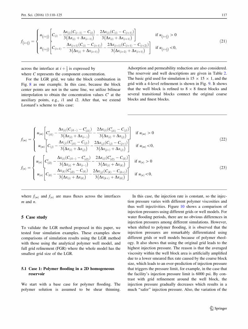
In this case, the injection rate is constant, so the injec-
tion pressure varies with different polymer viscosities and
thus well injectivities. Figure 10 shows a comparison of
injection pressures using different grids or well models. For
water flooding periods, there are no obvious differences in
injection pressures among different simulations. However,
when shifted to polymer flooding, it is observed that the
injection pressures are remarkably differentiated using
different grids or well models because of polymer rheol-
ogy. It also shows that using the original grid leads to the
highest injection pressure. The reason is that the averaged
viscosity within the well block area is artificially amplified
due to a lower smeared flux rate caused by the coarse block
size, which leads to an over-prediction of injection pressure
that triggers the pressure limit, for example, in the case that
the facility’s injection pressure limit is 6000 psi. By con-
trast with grid refinement around the well block, the
injection pressure gradually decreases which results in a
much ‘‘safer’’ injection pressure. Also, the variation of the
fiþ1
2ð Þ ¼u
iþ12ð Þ C ið Þ �
Dx ið ÞðC i�1ð Þ � C ið ÞÞ3 Dx ið Þ þ Dx i�1ð Þ� � �
2Dx ið ÞðC ið Þ � C iþ1ð ÞÞ3 Dx ið Þ þ Dx iþ1ð Þ� �
" #if u
iþ12ð Þ[ 0
uiþ1
2ð Þ C iþ1ð Þ �Dx iþ1ð ÞðC ið Þ � C iþ1ð ÞÞ3 Dx ið Þ þ Dx iþ1ð Þ� � �
2Dx iþ1ð ÞðC iþ1ð Þ � C iþ2ð ÞÞ3 Dx iþ2ð Þ þ Dx iþ1ð Þ� �
" #if u
iþ12ð Þ\0;
8>>>><
>>>>:
ð21Þ
f mð Þ ¼u mð Þ C0
i1ð Þ �Dx ið ÞðC i1�ð Þ � C0
i1ð ÞÞ3 Dx ið Þ þ Dx i�ð Þ� � �
2Dx ið ÞðC0i1ð Þ � C jð ÞÞ
3 Dx ið Þ þ Dx jð Þ� �
" #if u mð Þ [ 0
u mð Þ C jð Þ �Dx jð ÞðC0
i1ð Þ � C jð ÞÞ3 Dx ið Þ þ Dx jð Þ� � �
2Dx jð ÞðC jð Þ � C jþð ÞÞ3 Dx jþð Þ þ Dx jð Þ� �
" #if u mð Þ\0;
8>>>><
>>>>:
ð22Þ
f nð Þ ¼u nð Þ C0
i2ð Þ �Dx ið ÞðC i1�ð Þ � C0
i2ð ÞÞ3 Dx ið Þ þ Dx i�ð Þ� � �
2Dx ið ÞðC0i2ð Þ � C kð ÞÞ
3 Dx ið Þ þ Dx kð Þ� �
" #if u nð Þ [ 0
u nð Þ C kð Þ �Dx kð ÞðC0
i2ð Þ � C kð ÞÞ3 Dx ið Þ þ Dx kð Þ� � �
2Dx jð ÞðC kð Þ � C kþð ÞÞ3 Dx kþð Þ þ Dx kð Þ� �
" #if u nð Þ\0;
8>>>><
>>>>:
ð23Þ
Pet. Sci. (2016) 13:110–125 117
123

injection pressure shrinks with an increase in the level of
grid refinement, showing a convergent trend. Because
simulation results using 3-level LGR and 4-level LGR are
relatively close and further refinement may lead to exces-
sive computational times, we regard the simulation result
of 4-level LGR as the reference result to evaluate other
simulations. Of course, it should be more precise to use the
fully refined grid as the reference. Nevertheless, Fig. 10
shows that 4-level FGR gives a very similar injection
pressure to the 4-level LGR. We also use the analytical
injectivity model (Li and Delshad 2014) and we observe
that the simulated injection pressure is between the results
of 3-level LGR and 4-level LGR. This result is more
accurate than the case without grid refinement and shows
consistency with LGR results.
To further demonstrate the accuracy and computa-
tional efficiency of the LGR method, we compare sim-
ulation results with CMG_STARS (2012). In the above
case, rheology parameters, Pa and c1/2, used in the
polymer rheology equation (Eq. 10), are set as 1.8 and
10 s-1, respectively. These parameters lead to a rela-
tively sharp shear-thinning curve. CMG_STARS uses a
different polymer rheology equation, which is a power-
law equation:
lapp ¼
l0p if uw\ulower
l0puw
ulower
nthin�1
if ulower\uw\uupper
l1 if uw [ uupper;
8>><
>>:ð24Þ
where nthin is the power-law exponent, and ulower is defined
by the point on the power-law curve when lapp is equal to
l0p: To be close to the UTCHEM polymer equation (Eq. 10)
for Case 1 using the CMG_STARS equation, we found out
that nthin must be small and it causes numerical stability
issues which are also indicated in the manual of
CMG_STARS (2012). Therefore, to achieve a relatively
similar polymer rheology curves for both simulators, we
use Pa = 1.5 and c1/2 = 3.8 s-1 for UTCHEM and
nthin = 0.5 and ulower = 0.02 ft/day for CMG_STARS.
Figure 11 shows a comparison of the results between
UTCHEM and CMG_STARS using the original grid,
4-level LGR, and 4-level FGR, respectively. It is found that
the injection pressure curves for the original grid match
very well between UTCHEM and CMG_STARS. In
Fig. 9 The mesh of the 4-level local grid refinement for Case 1
Table 2 Reservoir and well
descriptions (Case 1)Model description Values
Reservoir size 450 ft 9 450 ft 9 10 ft
No. of gridblocks 15 9 15 9 1
Simulation time, day 365
Number of components 3
Permeability in the x or y directions, mD 300
Initial water saturation 0.35
Polymer rheology exponent Pa 1.8
Shear rate at half zero-rate viscosity chf, s-1 10
Wells 1 injector; 1 producer
Injection rate, ft3/day 500
Producer bottomhole pressure (BHP), psi 1000
Water injection 0–150 and 270–365 days
Polymer injection 150–270 days (0.3 wt%)
118 Pet. Sci. (2016) 13:110–125
123
addition, the 4-level LGR simulation results of UTCHEM
and CMG_STARS are also close, with only a minor dif-
ference. This is acceptable because CMG_STARS and
UTCHEM use different polymer concentration-dependent
viscosity models and shear-thinning models as mentioned
in Goudarzi et al. (2013a). Again, for FGR results, we
observe both UTCHEM and CMG_STARS match well
with LGR results.
In Table 3, we compare the CPU times taken by
UTCHEM and CMG_STARS using different grids. For
both simulators, we use the same maximum time step
(0.01 day) and the same numerical scheme (IMPES) on the
same computer for the sake of consistency. We can see that
CMG_STARS takes about 3 times that of UTCHEM for
the original coarse grid, 2.5 times for the 4-level LGR, and
2.2 times for the 4-level FGR. An increase in CPU times is
also in the same order of the increase in gridblock numbers.
LGR shows very good computational efficiency compared
to FGR. Actually, CMG_STARS can take larger time steps
because it can use an adaptive implicit scheme. Therefore,
the purpose of the comparison is not to tell which simulator
is better in performance but to obtain a sense of the scaling
of the CPU times using LGR and FGR. In fact, the
advantage of using UTCHEM for modeling polymer flood
is that it has more comprehensive polymer models than
CMG_STARS, such as more options of rheology models
and stricter concentration-dependent and salinity-depen-
dent polymer, and near-well-corrected viscosity models.
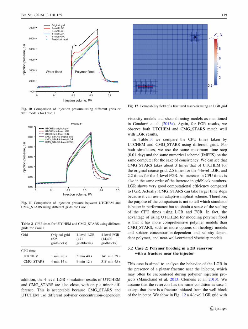
5.2 Case 2: Polymer flooding in a 2D reservoir
with a fracture near the injector
This case is aimed to analyze the behavior of the LGR in
the presence of a planar fracture near the injector, which
may often be encountered during polymer injection pro-
jects (Manichand et al. 2013; Clemens et al. 2013). We
assume that the reservoir has the same condition as case 1
except that there is a fracture initiated from the well block
of the injector. We show in Fig. 12 a 4-level LGR grid with
Fig. 12 Permeability field of a fractured reservoir using an LGR grid
Table 3 CPU times for UTCHEM and CMG_STARS using different
grids for Case 1
Grid Original grid
(225
gridblocks)
4-level LGR
(471
gridblocks)
4-level FGR
(14,400
gridblocks)
CPU time
UTCHEM 1 min 26 s 3 min 40 s 141 min 39 s
CMG_STARS 4 min 14 s 9 min 12 s 318 min 45 s
Original grid2-level LGR3-level LGR4-level LGR4-level FGRAnalytical moel
7000
6000
5000
4000
3000
2000
1000
Inje
ctio
n pr
essu
re, p
si
Water flood Polymer flood
0 0.1 0.2 0.3 0.4
Injection volume, PV
Fig. 10 Comparison of injection pressure using different grids or
well models for Case 1
7000
6000
5000
4000
3000
2000
1000
Inje
ctio
n pr
essu
re, p
si
0 0.1 0.2 0.3 0.4
Injection volume, PV0.5
UTCHEM original gridUTCHEM 4-level LGRUTCHEM 4-level FGRCMG_STARS original gridCMG_STARS 4-level LGRCMG_STARS 4-level FGR
PWB1 BHP
Fig. 11 Comparison of injection pressure between UTCHEM and
CMG_STARS using different grids for Case 1
Pet. Sci. (2016) 13:110–125 119
123

permeability field (the fracture permeability is assumed to
be 10 Darcy). In this case, it is obviously not proper to use
the coarse grid as well as the analytical injectivity model,
which could not describe the flow in fractures. Therefore, it
is obligatory to refine the gridblocks.
Figure 13 shows simulation results under three condi-
tions: LGR without fractures, LGR with fractures, and FGR
with fractures. The LGR with fractures leads to a signifi-
cantly smaller injection pressure compared to the LGR
without fractures, which shows the importance of
accounting for fractures near the injector. We also show
that the pressure curve of FGR is close to that of LGR,
which proves the agreement of the results between using
the two types of grids.
5.3 Case 3: Polymer flooding in a 3D heterogeneous
reservoir
We study a polymer flooding field case. The polymer
solution is assumed to be shear thinning. Adsorption and
permeability reduction are also considered. The reservoir
and well descriptions are given in Table 4. The perme-
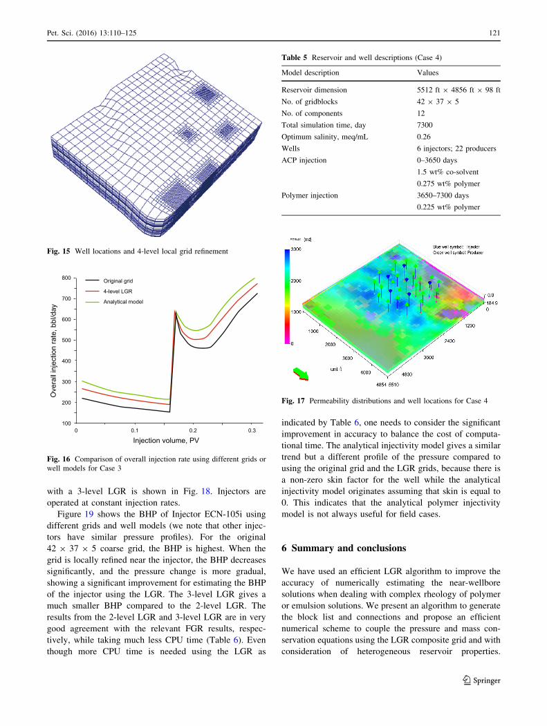
ability field and well locations are shown in Fig. 14. The
relevant grid with 4-level LGR is in Fig. 15. Some wells
are deviated so that the LGR is expanded in the x–y plane.
In this case, the injection pressure is fixed so that the
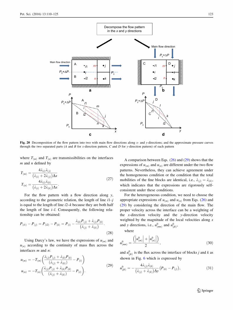
injection rate varies with well injectivity. Figure 16 shows
the simulated overall injection rate using the original grid,
4-level LGR, and the analytical injectivity model. It is
observed that we achieve a higher injection rate with grid
refinement compared to the original grid, which is con-
sistent with the polymer rheology. This is significant since
we need to accurately calculate how high a polymer vis-
cosity can be injected and the predicted bottomhole pres-
sure (BHP) for cases that the operators do not plan to inject
polymer above the fracture gradient. In this case, we lack
the results of FGR because of the excessive simulation
time. It is observed that the analytical model slightly
overestimates the overall injection rate compared to 4-level
LGR. The analytical model is not accurate for this case
because the well is inclined.
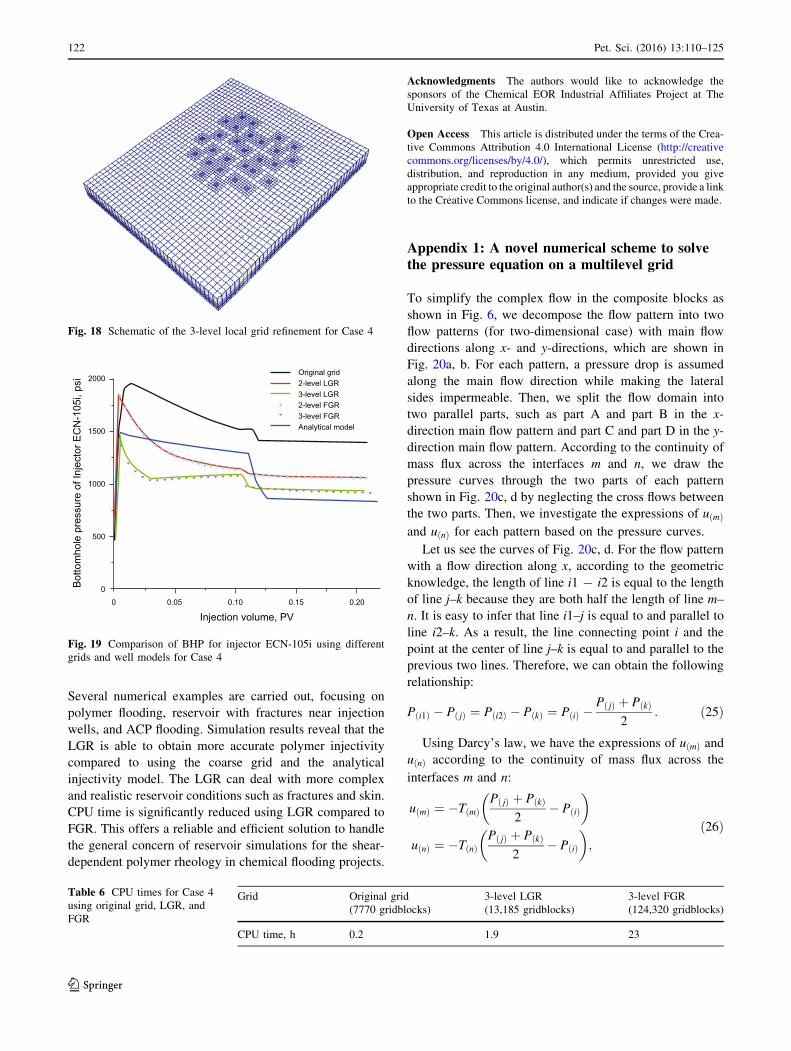
5.4 Case 4: A pilot of alkaline co-solvent polymer
(ACP) flood
The reservoir is a sandstone reservoir at a depth of
approximately 1000 ft which has undergone water flooding
for several years. The average oil saturation before ACP
flood is approximately 44.3 %. The pilot area includes 6
inverted 7-spot well patterns. The polymer solution is
assumed to be shear thinning. The reservoir and well
descriptions are given in Table 5. The permeability field
and well locations are shown in Fig. 17. The relevant grid
Fig. 14 Permeability distribution and well locations for Case 3
Table 4 Reservoir and well descriptions (Case 3)
Model description Values
No. of gridblocks 17 9 21 9 25
No. of components 6
Total injection volume for simulation,
PV
0.32
Polymer injection volume, PV 0–0.16 (0.2 wt%)
Water injection volume, PV 0.16–0.32
BHP, psi Injectors 4500; Producers
700
4-level LGR without fractures
4-level LGR with fractures
4-level FGR with fractures
6000
5000
4000
3000
2000
1000
Bot
tom
hole
pre
ssur
e, p
si
0 0.1 0.2 0.3 0.4
Injection volume, PV
Fig. 13 Comparison of injector bottomhole pressure (BHP) using
different grids or well models for Case 2
120 Pet. Sci. (2016) 13:110–125
123
with a 3-level LGR is shown in Fig. 18. Injectors are
operated at constant injection rates.
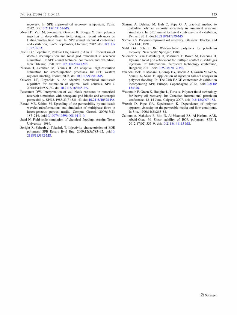
Figure 19 shows the BHP of Injector ECN-105i using
different grids and well models (we note that other injec-
tors have similar pressure profiles). For the original
42 9 37 9 5 coarse grid, the BHP is highest. When the
grid is locally refined near the injector, the BHP decreases
significantly, and the pressure change is more gradual,
showing a significant improvement for estimating the BHP
of the injector using the LGR. The 3-level LGR gives a
much smaller BHP compared to the 2-level LGR. The
results from the 2-level LGR and 3-level LGR are in very
good agreement with the relevant FGR results, respec-
tively, while taking much less CPU time (Table 6). Even
though more CPU time is needed using the LGR as
indicated by Table 6, one needs to consider the significant
improvement in accuracy to balance the cost of computa-
tional time. The analytical injectivity model gives a similar
trend but a different profile of the pressure compared to
using the original grid and the LGR grids, because there is
a non-zero skin factor for the well while the analytical
injectivity model originates assuming that skin is equal to
0. This indicates that the analytical polymer injectivity
model is not always useful for field cases.
6 Summary and conclusions
We have used an efficient LGR algorithm to improve the
accuracy of numerically estimating the near-wellbore
solutions when dealing with complex rheology of polymer
or emulsion solutions. We present an algorithm to generate
the block list and connections and propose an efficient
numerical scheme to couple the pressure and mass con-
servation equations using the LGR composite grid and with
consideration of heterogeneous reservoir properties.
Table 5 Reservoir and well descriptions (Case 4)
Model description Values
Reservoir dimension 5512 ft 9 4856 ft 9 98 ft
No. of gridblocks 42 9 37 9 5
No. of components 12
Total simulation time, day 7300
Optimum salinity, meq/mL 0.26
Wells 6 injectors; 22 producers
ACP injection 0–3650 days
1.5 wt% co-solvent
0.275 wt% polymer
Polymer injection 3650–7300 days
0.225 wt% polymer
Fig. 15 Well locations and 4-level local grid refinement
Original grid
4-level LGR
Analytical model
800
700
600
500
400
300
200
100
Ove
rall
inje
ctio
n ra
te, b
bl/d
ay
0 0.1 0.2 0.3
Injection volume, PV
Fig. 16 Comparison of overall injection rate using different grids or
well models for Case 3
Fig. 17 Permeability distributions and well locations for Case 4
Pet. Sci. (2016) 13:110–125 121
123
Several numerical examples are carried out, focusing on
polymer flooding, reservoir with fractures near injection
wells, and ACP flooding. Simulation results reveal that the
LGR is able to obtain more accurate polymer injectivity
compared to using the coarse grid and the analytical
injectivity model. The LGR can deal with more complex
and realistic reservoir conditions such as fractures and skin.
CPU time is significantly reduced using LGR compared to
FGR. This offers a reliable and efficient solution to handle
the general concern of reservoir simulations for the shear-
dependent polymer rheology in chemical flooding projects.
Acknowledgments The authors would like to acknowledge the
sponsors of the Chemical EOR Industrial Affiliates Project at The
University of Texas at Austin.
Open Access This article is distributed under the terms of the Crea-
tive Commons Attribution 4.0 International License (http://creative
commons.org/licenses/by/4.0/), which permits unrestricted use,
distribution, and reproduction in any medium, provided you give
appropriate credit to the original author(s) and the source, provide a link
to the Creative Commons license, and indicate if changes were made.
Appendix 1: A novel numerical scheme to solvethe pressure equation on a multilevel grid
To simplify the complex flow in the composite blocks as
shown in Fig. 6, we decompose the flow pattern into two
flow patterns (for two-dimensional case) with main flow
directions along x- and y-directions, which are shown in
Fig. 20a, b. For each pattern, a pressure drop is assumed
along the main flow direction while making the lateral
sides impermeable. Then, we split the flow domain into
two parallel parts, such as part A and part B in the x-
direction main flow pattern and part C and part D in the y-
direction main flow pattern. According to the continuity of
mass flux across the interfaces m and n, we draw the
pressure curves through the two parts of each pattern
shown in Fig. 20c, d by neglecting the cross flows between
the two parts. Then, we investigate the expressions of uðmÞand uðnÞ for each pattern based on the pressure curves.
Let us see the curves of Fig. 20c, d. For the flow pattern
with a flow direction along x, according to the geometric
knowledge, the length of line i1 - i2 is equal to the length
of line j–k because they are both half the length of line m–
n. It is easy to infer that line i1–j is equal to and parallel to
line i2–k. As a result, the line connecting point i and the
point at the center of line j–k is equal to and parallel to the
previous two lines. Therefore, we can obtain the following
relationship:
P i1ð Þ � P jð Þ ¼ P i2ð Þ � P kð Þ ¼ P ið Þ �P jð Þ þ P kð Þ
2: ð25Þ
Using Darcy’s law, we have the expressions of uðmÞ anduðnÞ according to the continuity of mass flux across the
interfaces m and n:
uðmÞ ¼ �TðmÞP jð Þ þ P kð Þ
2� P ið Þ
� �
uðnÞ ¼ �TðnÞP jð Þ þ P kð Þ
2� P ið Þ
� �;
ð26Þ
Table 6 CPU times for Case 4
using original grid, LGR, and
FGR
Grid Original grid
(7770 gridblocks)
3-level LGR
(13,185 gridblocks)
3-level FGR
(124,320 gridblocks)
CPU time, h 0.2 1.9 23
Fig. 18 Schematic of the 3-level local grid refinement for Case 4
Original grid2-level LGR3-level LGR2-level FGR3-level FGRAnalytical model
2000
1500
1000
500
0Bot
tom
hole
pre
ssur
e of
Inje
ctor
EC
N-1
05i,
psi
0 0.05 0.10 0.15 0.20
Injection volume, PV
Fig. 19 Comparison of BHP for injector ECN-105i using different
grids and well models for Case 4
122 Pet. Sci. (2016) 13:110–125
123
where TðmÞ and TðnÞ are transmissibilities on the interfaces
m and n defined by
T mð Þ ¼4k ið Þk jð Þ
k ið Þ þ 2k jð Þ� �
Dx
T nð Þ ¼4k ið Þk kð Þ
k ið Þ þ 2k kð Þ� �
Dx:
ð27Þ
For the flow pattern with a flow direction along y,
according to the geometric relation, the length of line i1–j
is equal to the length of line i2–k because they are both half
the length of line i–l. Consequently, the following rela-
tionship can be obtained:
P i1ð Þ � P jð Þ ¼ P i2ð Þ � P kð Þ ¼ P ið Þ �k kð ÞP jð Þ þ k jð ÞP kð Þ
k jð Þ þ k kð Þ� � :
ð28Þ
Using Darcy’s law, we have the expressions of uðmÞ anduðnÞ according to the continuity of mass flux across the
interfaces m and n:
uðmÞ ¼ �TðmÞk jð ÞP jð Þ þ k kð ÞP kð Þ
ðk jð Þ þ k kð ÞÞ� P ið Þ
� �
uðnÞ ¼ �TðnÞk jð ÞP jð Þ þ k kð ÞP kð Þ
ðk jð Þ þ k kð ÞÞ� P ið Þ
� �:
ð29Þ
A comparison between Eqs. (26) and (29) shows that the
expressions of uðmÞ and uðnÞ are different under the two flow
patterns. Nevertheless, they can achieve agreement under
the homogeneous condition or the condition that the total
mobilities of the fine blocks are identical, i.e., k jð Þ ¼ k kð Þ,
which indicates that the expressions are rigorously self-
consistent under these conditions.
For the heterogeneous condition, we need to choose the
appropriate expressions of uðmÞ and uðnÞ from Eqs. (26) and
(29) by considering the direction of the main flow. The
proper velocity across the interface can be a weighting of
the x-direction velocity and the y-direction velocity
weighted by the magnitude of the local velocities along x
and y directions, i.e., u0ðmnÞ and u0ðjkÞ,
where
u0ðmnÞ ¼u0ðmÞ
������þ u0ðnÞ
������
� �
2; ð30Þ
and u0ðjkÞ is the flux across the interface of blocks j and k as
shown in Fig. 6 which is expressed by
u0ðjkÞ ¼ �4k jð Þk kð Þ
k jð Þ þ k kð Þ� �
DyP kð Þ � P jð Þ� �
; ð31Þ
Decompose the flow patternin the x and y directions
Main flow direction
P0+∆P
A
B
i1
i
i2
m
n
j
k
P0
Main flow direction
P0+∆P
i1
i
i2
m
n
C Dj
k
li
P0
a b
c d
P0+∆P
P0
P
A
B
D
C
i1i
i2
m
n
j
kx
P
P0+∆P
P0
i1
i
i2
jI
k
y
Fig. 20 Decomposition of the flow pattern into two with main flow directions along x- and y-directions; and the approximate pressure curves
through the two separated parts (A and B for x-direction pattern, C and D for y-direction pattern) of each pattern
Pet. Sci. (2016) 13:110–125 123
123

where the superscript 0 for the velocities represents the last
time step.
Therefore, we design the following numerical scheme to
calculate uðmÞ and uðnÞ:
We are aware that this numerical scheme is achieved
based on the assumption that the cross flows between the
separated parts for each flow pattern can be neglected.
Actually, the piece-wise pressure curves shown in Fig. 20
may be bent when there is cross flow vertical to the main
flow direction. Nevertheless, this numerical scheme has a
lot of advantages that will be discussed in the text.
References
Bekbauov BE, Kaltayev A, Wojtanowicz AK, Panfilov M. Numerical
modeling of the effects of disproportionate permeability reduc-
tion water-shutoff treatments on water coning. J Energy Res
Technol. 2013;135(1):011101. doi:10.1115/1.4007913.
Berger MJ, Oliger J. Adaptive mesh refinement for hyperbolic partial
differential equations. J Comput Phys. 1984;53(3):484–512.
doi:10.1016/0021-9991(84)90073-1.
Cannella WJ, Huh C, Seright RS. Prediction of xanthan rheology in
porous media. In: SPE annual technical conference and exhibi-
tion, Houston, TX; 1998. doi:10.2118/18089-MS.
Carreau PJ. Rheological equations from molecular network theories.
PhD dissertation, University of Wisconsin-Madison. 1968.
Christensen JR, Darche G, Dechelette B, Ma H, Sammon PH.
Applications of dynamic gridding to thermal simulations. In:
SPE international thermal operations and heavy oil symposium
and western regional meeting, Bakersfield; 2004. doi:10.2118/
86969-MS.
Clemens T, Deckers M, Kornberger M, Gumpenberger T, Zechner M.
Polymer solution injection-near wellbore dynamics and dis-
placement efficiency, pilot test results, Matzen Field, Austria. In:
EAGE annual conference and exhibition incorporating SPE
Europec, London; 2013. doi:10.2118/164904.
Computing Modeling Group Ltd. User’s guide STARS: Advanced
Process and Thermal Reservoir Simulator, Calgary, AB; 2012.
Delshad M, Pope GA, Sepehrnoori K. A compositional simulator for
modeling surfactant enhanced aquifer remediation, 1. Formula-
tion. J Contam Hydrol. 1996;23(4):303–27. doi:10.1016/0169-
7722(95)00106-9.
Delshad M, Kim D, Magbagbeola O, Huh C, Pope G, Tarahhom F.
Mechanistic interpretation and utilization of viscoelastic behav-
ior of polymer solutions for improved polymer-flood efficiency.
In: SPE symposium on improved oil recovery, Tulsa; 2008.
doi:10.2118/113620-MS.
Forsyth PA, Sammon PH. Local mesh refinement and modeling of
faults and pinchouts. SPE For Eval. 1986;1(3):275–85. doi:10.
2118/13524-PA.
Gadde P, Sharma M. Growing injection well fractures and their impact
on waterflood performance. In: SPE annual technical conference
and exhibition, New Orleans; 2001. doi:10.2118/71614-MS.
Gerritsen M, Lambers JV. Integration of local-global upscaling and
grid adaptivity for simulation of subsurface flow in heteroge-
neous formations. Comput Geosci. 2008;12(2):193–208. doi:10.
1007/s10596-007-9078-2.
Goudarzi A, Delshad M, Sepehrnoori K. A critical assessment of
several reservoir simulators for modeling chemical enhanced oil
recovery processes. In: SPE reservoir simulation symposium,
Woodlands; 2013a. doi:10.2118/163578-MS.
Goudarzi A, Zhang H, Varavei A, Hu Y, Delshad M, Bai B,
Sepehrnoori K. Water management in mature oil fields using
preformed particle gels. In: SPE Western Regional AAPG
Pacific Section meeting, 2013 Joint Technical Conference,
Monterey; 2013b. doi:10.2118/165356.
Karimi-Fard M, Durlofsky L. Accurate resolution of near-well effects
in upscaled models using flow based unstructured local grid
refinement. SPE J. 2012;17(4):1084–95. doi:10.2118/141675-
PA.
Kulawardana E, Koh H, Kim DH, Liyanage P, Upamali K, Huh C,
Weerasooriya U, Pope G. Rheology and transport of improved
EOR polymers under harsh reservoir conditions. In: SPE
improved oil recovery symposium, Tulsa; 2012. doi:10.2118/
154294-MS.
Lee K, Huh C, Sharma M. Impact of fractures growth on well
injectivity and reservoir sweep during waterflood and chemical
EOR processes. In: SPE annual technical conference and
exhibition, Denver; 2011. doi:10.2118/146778-MS.
Li Z, Delshad M. Development of an analytical injectivity model for
non-Newtonian polymer solutions. SPE J. 2014;19(3):381–9.
doi:10.2118/163672-MS.
Liu J, Delshad M, Pope GA, Sepehrnoori K. Application of higher-
order flux-limited methods in compositional simulation. Transp
Porous Media. 1994;16(1):1–29. doi:10.1007/BF01059774.
Manichand RN, Let MS, Kathleen P, Gil L, Quillien B, Seright RS.
Effective propagation of HPAM solutions through the Tam-
baredjo reservoir during a polymer flood. SPE Prod Oper.
2013;28(4):358–68. doi:10.2118/164121-PA.
Meter DM, Bird RB. Tube flow of non-Newtonian polymer solutions:
part I. Laminar flow and rheological models. AIChE J.
1964;10(6):878–81. doi:10.1002/aic.690100619.
Mohammadi H, Jerauld G. Mechanistic modeling of the benefit of
combining polymer with low salinity water for enhanced oil
u mð Þ ¼ �T mð ÞP jð Þ þ P kð Þ
2� P ið Þ
� �u0mnð Þ
u0mnð Þ þ u0
jkð Þþ
k jð ÞP jð Þ þ k kð ÞP kð Þðk jð Þ þ k kð ÞÞ
� P ið Þ
� �u0jkð Þ
u0mnð Þ þ u0
jkð Þ
" #
u nð Þ ¼ �TðnÞP jð Þ þ P kð Þ
2� P ið Þ
� �u0
mnð Þ
u0mnð Þ þ u0
jkð Þþ
k jð ÞP jð Þ þ k kð ÞP kð Þðk jð Þ þ k kð ÞÞ
� P ið Þ
� �u0
jkð Þ
u0mnð Þ þ u0
jkð Þ
" #:
8>>>>><
>>>>>:
ð32Þ
124 Pet. Sci. (2016) 13:110–125
123
recovery. In: SPE improved oil recovery symposium, Tulsa;
2012. doi:10.2118/153161-MS.
Morel D, Vert M, Jouenne S, Gauchet R, Bouger Y. First polymer
injection in deep offshore field, Angola: recent advances on
Dalia/Camelia field case. In: SPE annual technical conference
and exhibition, 19–22 September, Florence; 2012. doi:10.2118/
135735-PA.
Nacul EC, Lepretre C, Pedrosa OA, Girard P, Aziz K. Efficient use of
domain decomposition and local grid refinement in reservoir
simulation. In: SPE annual technical conference and exhibition,
New Orleans; 1990. doi:10.2118/20740-MS.
Nilsson J, Gerritsen M, Younis R. An adaptive, high-resolution
simulation for steam-injection processes. In: SPE western
regional meeting, Irvine; 2005. doi:10.2118/93881-MS.
Oliveira DF, Reynolds A. An adaptive hierarchical multiscale
algorithm for estimation of optimal well controls. SPE J.
2014;19(5):909–30. doi:10.2118/163645-PA.
Peaceman DW. Interpretation of well-block pressures in numerical
reservoir simulation with nonsquare grid blocks and anisotropic
permeability. SPE J. 1983;23(3):531–43. doi:10.2118/10528-PA.
Rasaei MR, Sahimi M. Upscaling of the permeability by multiscale
wavelet transformations and simulation of multiphase flows in
heterogeneous porous media. Comput Geosci. 2009;13(2):
187–214. doi:10.1007/s10596-008-9111-0.
Saad N. Field-scale simulation of chemical flooding. Austin: Texas
University; 1989.
Seright R, Seheult J, Talashek T. Injectivity characteristics of EOR
polymers. SPE Reserv Eval Eng. 2009;12(5):783–92. doi:10.
2118/115142-MS.
Sharma A, Delshad M, Huh C, Pope G. A practical method to
calculate polymer viscosity accurately in numerical reservoir
simulators. In: SPE annual technical conference and exhibition,
Denver; 2011. doi:10.2118/147239-MS.
Sorbie KS. Polymer-improved oil recovery. Glasgow: Blackie and
Son Ltd.; 1991.
Stahl GA, Schulz DN. Water-soluble polymers for petroleum
recovery. New York: Springer; 1988.
Suicmez V, van Batenburg D, Matsuura T, Bosch M, Boersma D.
Dynamic local grid refinement for multiple contact miscible gas
injection. In: International petroleum technology conference,
Bangkok; 2011. doi:10.2523/15017-MS.
van den Hoek PJ, Mahani H, Sorop TG, Brooks AD, Zwaan M, Sen S,
Shuaili K, Saadi F. Application of injection fall-off analysis in
polymer flooding. In: The 74th EAGE conference & exhibition
incorporating SPE Europe, Copenhagen; 2012. doi:10.2118/
154376.
Wassmuth F, Green K, Hodgins L, Turta A. Polymer flood technology
for heavy oil recovery. In: Canadian international petroleum
conference, 12–14 June, Calgary; 2007. doi:10.2118/2007-182.
Wreath D, Pope GA, Sepehrnoori K. Dependence of polymer
apparent viscosity on the permeable media and flow conditions.
In Situ. 1990;14(3):263–84.
Zaitoun A, Makakou P, Blin N, Al-Maamari RS, Al-Hashmi AAR,
Abdel-Goad M. Shear stability of EOR polymers. SPE J.
2012;17(02):335–9. doi:10.2118/141113-MS.
Pet. Sci. (2016) 13:110–125 125
123


