Outline
Numerical experiments with additive Schwarzpreconditioner for non-overlapping domain
decomposition in 3D
Azzam Haidar
CERFACS, Toulouse
joint work with
Luc Giraud (N7-IRIT, France) and Shane Mulligan (Dublin Institute of Technology, Ireland)
4th International Workshop on Parallel Matrix Algorithms and Applications,
September 7-9, 2006, IRISA, Rennes, France
1/21 Numerical experiments with additive Schwaz preconditioner

Outline
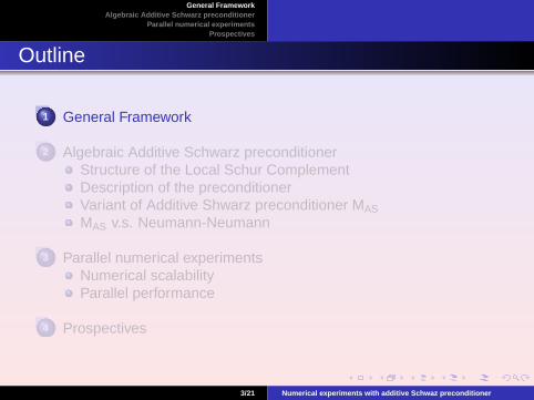
Outline
1 General Framework
2 Algebraic Additive Schwarz preconditionerStructure of the Local Schur ComplementDescription of the preconditionerVariant of Additive Shwarz preconditioner MAS
MAS v.s. Neumann-Neumann
3 Parallel numerical experimentsNumerical scalabilityParallel performance
4 Prospectives
2/21 Numerical experiments with additive Schwaz preconditioner
General FrameworkAlgebraic Additive Schwarz preconditioner
Parallel numerical experimentsProspectives
Outline
1 General Framework
2 Algebraic Additive Schwarz preconditionerStructure of the Local Schur ComplementDescription of the preconditionerVariant of Additive Shwarz preconditioner MAS
MAS v.s. Neumann-Neumann
3 Parallel numerical experimentsNumerical scalabilityParallel performance
4 Prospectives
3/21 Numerical experiments with additive Schwaz preconditioner

General FrameworkAlgebraic Additive Schwarz preconditioner
Parallel numerical experimentsProspectives
Background
The PDE 8<:−div(K .∇u) = f in Ω
u = 0 on ∂ΩDirichlet
(K∇u, n) = 0 on ∂ΩNeumann
The associated linear system
Au = f ≡
0@A11 A1Γ 0AT
1Γ A(1)Γ + A(2)
Γ AT2Γ
0 A2Γ A22
1A0@u1
u2
uΓ
1A =
0@f1f2fΓ
1A4/21 Numerical experiments with additive Schwaz preconditioner

Background
Algebraic splitting and block Gaussian elimination: N sub-domains case0BBB@AI1I1 . . . 0 AI1Γ1
.... . .
......
0 . . . AIN IN AIN ΓN
AΓ1I1 . . . AΓN IN AΓΓ
1CCCA0BBB@
uI1...
uINuΓ
1CCCA =
0BBB@fI1...
fINfΓ
1CCCASuΓ =
NX
i=1
RTΓi
S(i)RΓi
!uΓ = fΓ −
NXi=1
RTΓi
AΓi Ii A−1Ii Ii
fIi
where S(i) = A(i)Γi Γi
− AΓi Ii A−1Ii Ii
AIi Γi
Spectral properties for elliptic PDE’s
κ(A) = O(h−2) κ(S) = O(h−1)
||e(k)||A ≤ 2 ·
pκ(A)− 1pκ(A) + 1
!k
||e(0)||A

General FrameworkAlgebraic Additive Schwarz preconditioner
Parallel numerical experimentsProspectives
Structure of the Local Schur ComplementDescription of the preconditionerVariant of Additive Shwarz preconditioner MASMAS v.s. Neumann-Neumann
Outline
1 General Framework
2 Algebraic Additive Schwarz preconditionerStructure of the Local Schur ComplementDescription of the preconditionerVariant of Additive Shwarz preconditioner MAS
MAS v.s. Neumann-Neumann
3 Parallel numerical experimentsNumerical scalabilityParallel performance
4 Prospectives
6/21 Numerical experiments with additive Schwaz preconditioner

General FrameworkAlgebraic Additive Schwarz preconditioner
Parallel numerical experimentsProspectives
Structure of the Local Schur ComplementDescription of the preconditionerVariant of Additive Shwarz preconditioner MASMAS v.s. Neumann-Neumann
Structure of the Local Schur Complement
Non-Overlapping Domain Decomposition
Ωi
Ωj
Ek
EgEm
E` Γi = E` ∪ Ek ∪ Em ∪ Eg
Distributed Schur Complement
S(i) =
0BBB@S(i)
mm Smg Smk Sm`
Sgm S(i)gg Sgk Sg`
Skm Skg S(i)kk Sk`
S`m S`g S`k S(i)``
1CCCA Sgg = S(i)gg + S(j)
gg
If A is SPD then S is also SPD⇒ CG
In a distributed memory environment: S is distributed non-assembled
7/21 Numerical experiments with additive Schwaz preconditioner

General FrameworkAlgebraic Additive Schwarz preconditioner
Parallel numerical experimentsProspectives
Structure of the Local Schur ComplementDescription of the preconditionerVariant of Additive Shwarz preconditioner MASMAS v.s. Neumann-Neumann
A simple mathematical framework
The local component
U a algebraic space of vectors associatedwith unknowns on Γ
Ui subspaces of U such thatU = U1 + ... + Un and
Ri : the canonical pointwise restriction fromU 7→ Ui
Mloc =n∑
i=1
RTi M−1
i Ri whereMi = RiSRTi
Examples :Ui associated with each edge: block JacobiUi associated with ∂Ωi : additive Schwarz
8/21 Numerical experiments with additive Schwaz preconditioner

General FrameworkAlgebraic Additive Schwarz preconditioner
Parallel numerical experimentsProspectives
Structure of the Local Schur ComplementDescription of the preconditionerVariant of Additive Shwarz preconditioner MASMAS v.s. Neumann-Neumann
Additive Schwarz preconditioner [ Carvalho, Giraud, Meurant, 01]
Preconditionner properties
Ui associated with the entire interface Γi of sub-domain ∂Ωi
MAS =
#domains∑i=1
RTi (S(i))−1Ri
S(i) =
0BB@Smm Smg Smk Sm`
Sgm Sgg Sgk Sg`
Skm Skg Skk Sk`
S`m S`g S`k S``
1CCAAssembled local Schur complement
S(i) =
0BBB@S(i)
mm Smg Smk Sm`
Sgm S(i)gg Sgk Sg`
Skm Skg S(i)kk Sk`
S`m S`g S`k S(i)``
1CCCAlocal Schur complement
RemarksMAS is SPD if S is SPD
9/21 Numerical experiments with additive Schwaz preconditioner

General FrameworkAlgebraic Additive Schwarz preconditioner
Parallel numerical experimentsProspectives
Structure of the Local Schur ComplementDescription of the preconditionerVariant of Additive Shwarz preconditioner MASMAS v.s. Neumann-Neumann
Cheaper Additive Shwarz preconditioner form
Main characteristics
Cheaper in memory space
FLOPS Reduction
Without any additional communication cost
Sparsification strategy
sij =
sij if sij ≥ ε(|sii |+ |sjj |)0 else
Mixed arithmetic strategy
Compute and store the preconditioner in single precisionarithmetic
10/21 Numerical experiments with additive Schwaz preconditioner

General FrameworkAlgebraic Additive Schwarz preconditioner
Parallel numerical experimentsProspectives
Structure of the Local Schur ComplementDescription of the preconditionerVariant of Additive Shwarz preconditioner MASMAS v.s. Neumann-Neumann
MAS v.s. Neumann-Neumann
Neumann-Neumann preconditioner[J.F Bourgat, R. Glowinski, P. Le Tallec and M. Vidrascu - 89]
[Y.H. de Roek, P. Le Tallec and M. Vidrascu - 91]
S(1) = S(2) =S2⇒ S−1 =
12
((S(1))−1 + (S(2))−1)12
A(i) =
„Aii AiΓ
AiΓ A(i)Γ
«=
„I 0
AiΓA−1ii I
«„Aii 00 S(i)
«„I A−1
ii AΓi
0 I
«(S(i))−1 =
`0 I
´(A(i))−1
„0I
«
MNN =
#domainsXi=1
RTi (Di(S
(i))−1Di)Ri while MAS =
#domainsXi=1
RTi (S(i))−1Ri
11/21 Numerical experiments with additive Schwaz preconditioner

General FrameworkAlgebraic Additive Schwarz preconditioner
Parallel numerical experimentsProspectives
Numerical scalabilityParallel performance
Outline
1 General Framework
2 Algebraic Additive Schwarz preconditionerStructure of the Local Schur ComplementDescription of the preconditionerVariant of Additive Shwarz preconditioner MAS
MAS v.s. Neumann-Neumann
3 Parallel numerical experimentsNumerical scalabilityParallel performance
4 Prospectives
12/21 Numerical experiments with additive Schwaz preconditioner

General FrameworkAlgebraic Additive Schwarz preconditioner
Parallel numerical experimentsProspectives
Numerical scalabilityParallel performance
Computational framework
Target computer
IBM-SP4 (CINES)
SGI O3800 (CINES)
Cray XD1 (CERFACS)
System X (Virginia Tech) jointly with Layne T. Watson-Virginia Polytechnic Institute
Local direct solver : MUMPS [Amestoy, Duff, Koster, L’Excellent - 01]
Main features- Parallel distributed multifrontal solver (F90, MPI)- Symmetric and Unsymmetric factorizations- Element entry matrices, distributed matrices- Efficient Schur complement calculation- Iterative refinement and backward error analysis
Public domain: new version 4.6.3www.enseeiht.fr/apo/MUMPS - [email protected]
13/21 Numerical experiments with additive Schwaz preconditioner

General FrameworkAlgebraic Additive Schwarz preconditioner
Parallel numerical experimentsProspectives
Numerical scalabilityParallel performance
Numerical scalability
3D Poisson problem:
Number of CG iterations where either:Hh constant while # sub-domains is varied horizontal view→
Increasing mesh size Hh while # sub-domains kept constant vertical view↓
# sub-domains ≡ # processorssub-domains size 27 64 125 216 343 512 729 1000
MAS 16 23 25 29 32 35 39 4220× 20× 20MSpAS 16 23 26 31 34 39 43 46MAS 17 24 26 31 33 37 40 4325× 25× 25
MSpAS 17 25 28 34 37 42 45 49MAS 18 25 27 32 34 39 42 4530× 30× 30
MSpAS 18 26 29 36 40 44 48 52MAS 19 26 30 33 35 43 44 4735× 35× 35
MSpAS 19 28 30 38 46 46 50 56
The solved problem size vary from 1.1 up to 42.8 Millions of unknowns
The number of iterations increases slightly when increasing # sub-domains
This increase is less significant when the local mesh size Hh grows
14/21 Numerical experiments with additive Schwaz preconditioner
General FrameworkAlgebraic Additive Schwarz preconditioner
Parallel numerical experimentsProspectives
Numerical scalabilityParallel performance
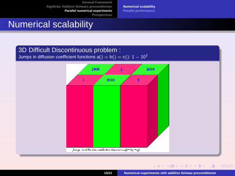
Numerical scalability
3D Difficult Discontinuous problem :Jumps in diffusion coefficient functions a() = b() = c(): 1− 103
15/21 Numerical experiments with additive Schwaz preconditioner

General FrameworkAlgebraic Additive Schwarz preconditioner
Parallel numerical experimentsProspectives
Numerical scalabilityParallel performance
Numerical scalability
3D Difficult Discontinuous problem :Jumps in diffusion coefficient functions a() = b() = c(): 1− 103
Number of CG iterations where either:Hh constant while # sub-domains is varied horizontal view→
Increasing mesh size Hh while # sub-domains kept constant vertical view↓
# sub-domains ≡ # processors
sub-domains size 27 64 125 216 343 512 729 1000
MAS 32 37 44 53 58 68 78 8220× 20× 20
MSpAS 32 42 48 58 63 75 85 91MAS 29 41 46 52 60 71 80 85
25× 25× 25MSpAS 34 45 51 63 66 82 89 99MAS 34 43 46 57 61 75 84 87
30× 30× 30MSpAS 30 47 52 68 70 90 96 105MAS 31 43 49 62 63 80 87 92
35× 35× 35MSpAS 29 51 58 71 84 92 105 116
16/21 Numerical experiments with additive Schwaz preconditioner

General FrameworkAlgebraic Additive Schwarz preconditioner
Parallel numerical experimentsProspectives
Numerical scalabilityParallel performance
Parallel performance
3D Difficult Discontinuous problem:
Implementation details:Setup Schur: MUMPS
Setup Precond: dense Schur(LAPACK)- sparse Schur(MUMPS)
Target computer : System Xserve MAC G5 - jointly with Layne T. Watson-Virginia
Polytechnic Institute
Parallel elapsed time: 103 processors Hh vary ε = 10−4
Jumps in diffusion coefficient functions a() = b() = c(): 1− 103
Sub-domains size 20× 20× 20 25× 25× 25 30× 30× 30 35× 35× 35
setup Schur 1.30 1.30 4.20 4.20 11.2 11.2 26.8 26.8
setup Precond 0.93 0.50 3.05 1.60 8.73 3.51 21.4 6.22
time per iter 0.08 0.05 0.23 0.13 0.50 0.28 0.77 0.37
total 8.79 6.17 26.8 18.6 63.0 44.1 119 75.9
# iter 82 91 85 99 87 105 92 116dense local Schur Precond MAS - sparse local Schur Precond MSpAS
17/21 Numerical experiments with additive Schwaz preconditioner
General FrameworkAlgebraic Additive Schwarz preconditioner
Parallel numerical experimentsProspectives
Numerical scalabilityParallel performance
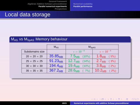
Local data storage
MAS vs MSpAS Memory behaviour
MAS MSpAS
Subdomains size ε = 10−5 ε = 10−4
20× 20× 20 35.85MB 7.5MB (10%) 1.8MB ( 5%)
25× 25× 25 91.23MB 12.7MB (14%) 2.7MB ( 3%)
30× 30× 30 194.4MB 19.4MB (10%) 3.8MB ( 2%)
35× 35× 35 367.2MB 28.6MB ( 7%) 10.2MB ( 2%)
18/21 Numerical experiments with additive Schwaz preconditioner
General FrameworkAlgebraic Additive Schwarz preconditioner
Parallel numerical experimentsProspectives
Outline
1 General Framework
2 Algebraic Additive Schwarz preconditionerStructure of the Local Schur ComplementDescription of the preconditionerVariant of Additive Shwarz preconditioner MAS
MAS v.s. Neumann-Neumann
3 Parallel numerical experimentsNumerical scalabilityParallel performance
4 Prospectives
19/21 Numerical experiments with additive Schwaz preconditioner

General FrameworkAlgebraic Additive Schwarz preconditioner
Parallel numerical experimentsProspectives
Prospectives
Objective
Control the growth of iterations when increasing the # processors
Various possibilities (future work)
Numerical remedy: two-level preconditioner- Coarse space correction, ie solve a closed problem on a coarse
space- Various choices for the coarse component (eg one d.o.f. per
sub-domain)
Computer Science remedy : several processors per sub-domain- two-level of parallelism- 2D cyclic data storage
20/21 Numerical experiments with additive Schwaz preconditioner

General FrameworkAlgebraic Additive Schwarz preconditioner
Parallel numerical experimentsProspectives
Numerical alternative: preleminary results
Domain based coarse space : M = MAS + RTOA−1
O R0
“As many” dof in the coarse space assub-domains [Carvalho, Giraud, Le Tallec, 01]
Partition of unity : RT0 simplest constant
interpolation
Anisotropic and Discontinuous 3D problem: Hh = 30
# procs 125 216 343 512 729 1000
setup Schur 11.2 11.2 11.2 11.2 11.2 11.2 11.2 11.2 11.2 11.2 11.2 11.2
setup Precond 8.70 8.70 8.70 8.70 8.70 8.70 8.70 8.70 8.70 8.70 8.70 8.70
setup coarse 0.80 - 0.83 - 0.87 - 0.92 - 0.96 - 1.30 -
time per iter 0.50 0.50 0.50 0.50 0.51 0.50 0.51 0.50 0.52 0.50 0.53 0.50
total 40.2 44.9 46.7 50.9 51.8 55.4 55.0 59.9 58.5 64.0 62.5 67.6
# iter 39 50 52 62 61 71 67 80 73 88 78 95with coarse space - without coarse space
21/21 Numerical experiments with additive Schwaz preconditioner

General FrameworkAlgebraic Additive Schwarz preconditioner
Parallel numerical experimentsProspectives
Parallel computing alternative
Main characteristics of the two-level of parallelism
Anisotropic and Discontinuous 3D problem: very preliminary result on-going work
# Sub-domains Sub-dom size # iter Setup Schur Setup MAS time/iter total time
1 Level 1000 20× 20× 20 186 1.30 0.95 0.08 17.0
2 Level 125 39× 39× 39 99 21.0 11.2 0.26 58.5
22/21 Numerical experiments with additive Schwaz preconditioner