NUMERICAL ANALYSIS AND PARAMETER STUDY OF A MECHANICAL DAMPER IN MACHINE TOOL
By
DONGKI WON
A THESIS PRESENTED TO THE GRADUATE SCHOOL OF THE UNIVERSITY OF FLORIDA IN PARTIAL FULFILLMENT
OF THE REQUIREMENTS FOR THE DEGREE OF MASTER OF SCIENCE
UNIVERSITY OF FLORIDA
2004

Copyright 2004
by
Dongki Won

ACKNOWLEDGMENTS
The researcher would like to express his gratitude to Dr. Nam Ho Kim for his
inspiration, support and guidance during this research. Thanks also go to other committee
members Dr. John Ziegert and Dr. Raphael Haftka for their support and service on the
author’s advisory committee. Special thanks go Mr. Charles Stanislaus and the students
in the design lab for their help in completing tasks associated with the research. Finally,
the author wishes to thank his wife, parents, and other family members. Without their
support and caring this work would not have been possible.
iii

TABLE OF CONTENTS
page ACKNOWLEDGMENTS ................................................................................................. iii
LIST OF TABLES............................................................................................................. vi
LIST OF FIGURES .......................................................................................................... vii
ABSTRACT....................................................................................................................... ix
CHAPTER 1 INTRODUCTION ........................................................................................................1
2 SIMPLIFIED MODEL .................................................................................................5
3 REVIEW OF ANALYTICAL APPROACH................................................................9
Calculation of the Normal Force and the Contact Pressure........................................10 Calculation of the Relative Displacement and the Work............................................16
4 BACKGROUND OF FINITE ELEMENTANALYSIS IN CONTACT
PROBLEMS ...............................................................................................................25
Contact Formulation in Static Problems.....................................................................26 The Lagrange Multiplier Method ...............................................................................29 The Penalty Method....................................................................................................30
5 FIITE ELEMENT ANALYSIS ..................................................................................32
Finite Element Model .................................................................................................32 Boundary Conditions ..................................................................................................35 Calculation of Friction Work......................................................................................36 Finite Element Analysis Results.................................................................................37
Load Step 1..........................................................................................................37 Load Step 2 (Centrifugal Force + Vertical Force)...............................................38
6 PARAMETER STUDY..............................................................................................41
Determination of the Mesh Size .................................................................................41
iv

Determination of the Start Angle................................................................................42 Parameter Study..........................................................................................................46 Change the Inner Radius of the Finger. ......................................................................46 Change the Number of the Finger ..............................................................................47 Final Results ...............................................................................................................48 Comparison between the Analytical and Numerical Results .....................................50
7 CONCLUSION AND FUTURE WORK ...................................................................53
APPENDIX A MATLAB CODE FOR THEORITICAL ANALYSIS...............................................55
B ANSYS INPUT FILE 01 ............................................................................................59
C ANSYS INPUT FILE 02 ............................................................................................61
D ANSYS INPUT FILE 03 ............................................................................................63
E ANSYS INPUT FILE 04 ............................................................................................65
F ANSYS INPUT FILE 05 ............................................................................................68
REFERENCES ..................................................................................................................72
BIOGRAPHICAL SKETCH .............................................................................................73
v

LIST OF TABLES
Table page 2-1. Material properties used for the shank and finger. .......................................................8
3-1. First moment Q of various quantities. ........................................................................13
5-1. The number of nodes and elements. ...........................................................................33
6-1. The results of parameter study....................................................................................48
vi

LIST OF FIGURES
Figure page 1-1. Chatter mark. ................................................................................................................1
2-1. Endmill and damper......................................................................................................5
2-2. Model.simplification.....................................................................................................6
2-3. Dimensions of geometry...............................................................................................7
3-1. Cross sectional area of the endmill system.................................................................11
3-2. Cross sectional area of the finger. ..............................................................................14
3-3. Cross sectional area of the finger. ..............................................................................15
3-4. Plot of work done by the friction force according to the change of the inner radius of finger. .......................................................................................................................22
3-5. Plot of work done by the friction force for varying start angles of the finger............23
3-6. Plot of the work done by the friction force for different numbers of fingers.. ...........23
5-1. Solid 95, 20 node solid element..................................................................................32
5-2. FEA model of the endmill using 20 node cubic elements and 8 node contact elements with boundary conditions. ........................................................................................33
5-3. 8-node contact and target element description. ..........................................................34
5-4. Force boundary conditions in each time step. ............................................................35
5-5. Diagram explaining how to calculate the damping work. ..........................................36
5-6. FEA result for load step 1...........................................................................................37
5-7. FEA result for load step 2...........................................................................................39
5-8. Schematic diagram of endmill behavior according to the applied forces...................40
6-1. Damping according to the number of elements..........................................................41
vii

6-2. Damping according to the position of the finger........................................................42
6-3. The maximum and the minimum values of the damping work for the given number of fingers. .................................................................................................................43
6-4. Relative displacement of the two-finger case.............................................................44
6-5. Relative displacement of five-finger case. .................................................................45
6-6. The first design variable. ............................................................................................46
6-7. The second design variable.........................................................................................46
6-8. The result of the parameter study in which the inner radius of finger was changed. .47
6-9. The result of the parameter study in which the number of fingers is changed...........48
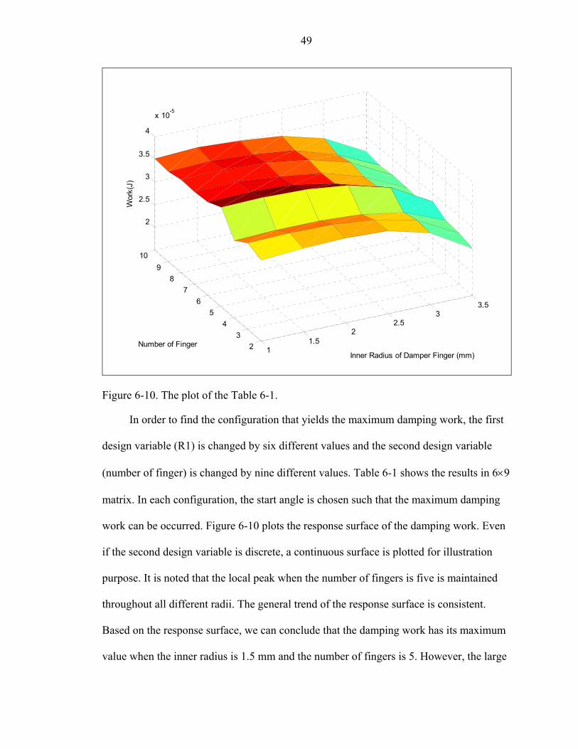
6-10. The plot of the Table 6-1. .........................................................................................49
viii

Abstract of Thesis Presented to the Graduate School
of the University of Florida in Partial Fulfillment of the Requirements for the Degree of Master of Science
NUMERICAL ANALYSIS AND PARAMETER STUDY OF A MECHANICAL DAMPER IN MACHINE TOOL
By
Dongki Won
May, 2004
Chair: Nam Ho Kim Major Department: Mechanical and Aerospace Engineering
When an endmill is used in high-speed machining, chatter vibration of the tool can
cause undesirable results. This vibration increases tool wear and leaves chatter marks on
the cutting surface. To reduce the chatter vibration, a layered-beam damper is inserted
into the hole at the center of the tool. The friction work done by the relative motion
between the tool and damper reduces chatter vibration. The purpose of this research is to
design and optimize the configuration of the damper to obtain the maximum damping
effect.
The analytical method has been reviewed, which is based on the assumption of
constant contact pressure and uniform deflection. For the numerical approach, nonlinear
finite element analysis is employed to calculate the distribution of the contact pressure
under the centrifugal and cutting forces. The analytical and numerical results are
compared and discussed.
ix

In order to identify the effect of the damper’s configuration, two design variables
are chosen: the inner radius of the damper and the number of slotted dampers. During the
parameter study and optimization, the inner radius is varied from 1.5mm to 3.5mm and
the number of slotted dampers is varied from 2 to 10.
Results show that the damping effect is maximum when the inner radius is 1.5mm
and the number of slotted dampers is 5. However, this result depends on the operating
condition. Thus, it is suggested to prepare a set of dampers and to apply the appropriate
one for the optimum damping effect for a given operating condition.
x

CHAPTER 1 INTRODUCTION
Milling is widely used in many areas of manufacturing. Traditionally, milling has
been regarded as a slow and costly process. Therefore, many efforts have been made to
improve the efficiency of milling. The main limitation of milling is caused by the
vibration of the machine tool and workpiece. As the speed and the power of milling are
increased, it is very important to control vibration of the tool.
Two different kinds of vibration affect the cutting operation. The one is the self-
excited (chatter) vibration at the high spindle speed, and the other is vibration at the
critical natural frequency. This research is focused on the former, which produces a wavy
surface during the milling operation, as shown in Fig.1-1.
Figure 1-1. Chatter mark.
Various methods of preventing chatter have been incorporated into machine tool
systems. In 1989, Cobb [2] developed dampers for boring bars. These dampers are
composed of two different types. The first type, which Cobb calls a shear damper, has
two end “caps” that fit snugly around a boring bar. Between these are sandwiched an
1

2
annular mass with plastic at each end, either in the form of ring or of several blocks at
each end. This middle section of a mass and plastic pieces has a clearance from the
boring bar, and is preloaded between the end caps with bolts. When the boring bar
vibrates, the end caps transmit this vibration through the plastic pieces to the annular
mass, which vibrates in tune. Since the plastic pieces do not slide on the faces of either
one, a shear force is produced on the end faces of the plastic. The viscoelastic properties
of the plastic provide damping for the system. The other type of damper proposed by
Cobb is the compression damper in which the mass is again an annulus. This annulus is
cut in half down its axis to form two half annuli. These are then bolted together around
rings of plastic that are in contact with the boring bar. The bolts provide a preload on the
plastic rings, and when the bar vibrates, the annular mass vibrates out of phase with it,
compressing one side and then the other of the plastic rings. This alternate squeezing of
the plastic creates damping, again by deforming the plastic, but in a compressive rather
than shearing manner.
In 1998, Dean [3] focused on increasing the depth of cut and increasing axis
federates to improve the metal removal rate (MRR). While he does not present any
original ideas on chatter reduction, his thesis refers to work done by Smith [6] in which a
chatter recognition system was developed. This system uses a microphone to detect the
frequency of chatter when it occurs. The system then selects a different speed(according
to the parameters of the system) and tries to machine again. This process repeats itself
until chatter no longer occurs.
Much work in the field of structural damping has been done by Slocum [5]. In
order to damp vibrations, Slocum uses layered beams with viscoelastic materials between

3
the layers. Two cantilevered beams are stacked on top of each other, and a force is
applied to the end of the top beam. It is known that beams experience an axial shear force
when displaced in this manner. Slocum’s derivation calculates a relative displacement
between corresponding points on the un-deformed beams. This is incorporated into a
selfdamping structure by placing several small beams inside of a larger beam and
injecting a viscoelastic material between them. This material bonds to each surface and
thus, when there is a relative displacement, is deformed. The stretching of this material
causes a dissipation of vibration energy and thus, damping.
In 2001, Sterling [7] explored the possibility of deploying a damper directly inside
of a rotating tool. To reduce the chatter vibration, a layered-beam damper, which Sterling
calls a finger, is inserted into the hole at the center of the tool. Due to the high-speed
rotation, the outer surface of the damper contacts with the inner surface of the tool. When
chatter vibration occurs, which is a deflection of the tool, work is done in the contact
interface due to the friction force and the relative motion. This work is dissipative and
reduces chatter vibration. He developed an analytical model and performed an
experiment for the layered beam damper.
In this research, the work done by Sterling is further extended. Using finite element
analysis, his analytical approach is compared to the numerical results. The objective of
this research is to calculate the amount of friction work and to maximize its effect by
changing the damper’s configuration.
The organization of thesis is as follows. In Chapter 2, a simplified model of the
endmill is introduced that can be used for analytical study and numerical simulation. In
Chapter 3, the analytical approach is reviewed that qualitatively estimates the damping

4
work. Chapter 4 presents the background knowledge of finite element analysis in contact
problems. Chapter 5 describes the numerical simulation procedure using the finite
element method. Chapter 6 represents the parameter study according to the change of two
design variables, followed by conclusions and future work at Chapter 7.
CHAPTER 2 SIMPLIFIED MODEL
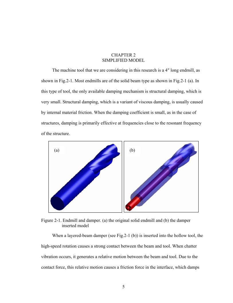
The machine tool that we are considering in this research is a 4″ long endmill, as
shown in Fig.2-1. Most endmills are of the solid beam type as shown in Fig.2-1 (a). In
this type of tool, the only available damping mechanism is structural damping, which is
very small. Structural damping, which is a variant of viscous damping, is usually caused
by internal material friction. When the damping coefficient is small, as in the case of
structures, damping is primarily effective at frequencies close to the resonant frequency
of the structure.
(b) (a)
Figure 2-1. Endmill and damper. (a) the original solid endmill and (b) the damper
inserted model
When a layered-beam damper (see Fig.2-1 (b)) is inserted into the hollow tool, the
high-speed rotation causes a strong contact between the beam and tool. When chatter
vibration occurs, it generates a relative motion between the beam and tool. Due to the
contact force, this relative motion causes a friction force in the interface, which damps
5

6
the vibration. In this research, this damping mechanism will be referred to as a
mechanical damper.
While the tool geometry is very important for cutting performance, the objective of
this research is on the vibration of the tool. Thus, we want to simplfy the tool geometry
so that the analytical and numerical studies in the following chapters will be convenient.
The first step of simplifying the endmill model is to suppress unnecessary
geometric details, while maintaining the endmill’s mechanical properties. The endmill
model can be simplified as a cylinder because we are only interested in the contact
surface, which is the inner surface of the tool. Fig.2-2 (b) illustrates the simplified model.
ω=2722.71 rad/s (a) (b)
F=100 N
Figure 2-2. Model simplification. (a) the detailed tool model in which the damper is
inserted and (b) the simplified model using hollowed cylinder.
The simplified endmill model is composed of two-hollowed cylinders. The outer
cylinder represents the endmill tool, and the inner cylinder represents the damper. For
convenience, the outer part (tool) is denoted as a shank, while the inner part (damper) is
denoted as a finger. As schematically illustrated in Fig.2-3, the outer radius R1 of the
finger is 1.5 mm, the inner radius R2 of the finger is 4.7625 mm, the inner radius R3 of
the shank is 4.7625 mm, and the outer radius R4 of the shank is 9.525 mm. The length of
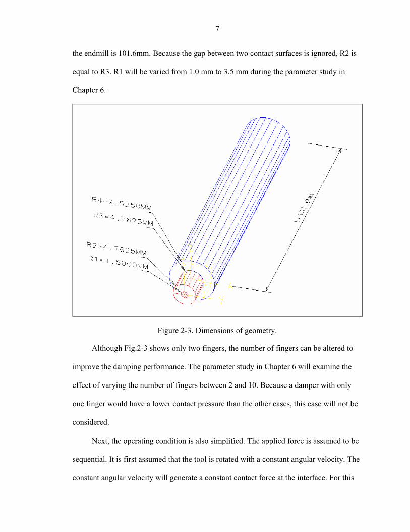
7
the endmill is 101.6mm. Because the gap between two contact surfaces is ignored, R2 is
equal to R3. R1 will be varied from 1.0 mm to 3.5 mm during the parameter study in
Chapter 6.
Figure 2-3. Dimensions of geometry.
Although Fig.2-3 shows only two fingers, the number of fingers can be altered to
improve the damping performance. The parameter study in Chapter 6 will examine the
effect of varying the number of fingers between 2 and 10. Because a damper with only
one finger would have a lower contact pressure than the other cases, this case will not be
considered.
Next, the operating condition is also simplified. The applied force is assumed to be
sequential. It is first assumed that the tool is rotated with a constant angular velocity. The
constant angular velocity will generate a constant contact force at the interface. For this

8
particular model, an angular velocity of 2,722.713rad/sec is used, which is equal to
26,000 rpm. In this initial state the endmill has not started cutting the surface. When the
endmill starts cutting the surface, the tool undergoes a vertical force at the end of the
endmill. To approximate the cutting process of the tool, a vertical force is applied at the
tip. To accurately approximate the cutting force, the vertical force on the endmill needs to
be measured and then an equal force needs be applied at the tip. However, since the
objective of this research is vibration control, a representative force of 100N is applied.
Thus, the damping work that will be calculated is not the actual magnitude, but rather a
relative quantity.
For simplicity, the same material properties are assumed for both the shank and
finger even though the stiffness of the finger is actually slightly higher than that of the
shank. The material properties used are listed in Table 2-1.
Table 2-1. Material properties used for the shank and finger. Material Property Value Young’s Modulus 206780 MPa
Mass Density 7.82×10⁻⁹ ton/mm3 Friction Coefficient 0.15
In the following chapters analytical and finite element analysis will use the
simplified model to determine the conditions for maximum damping of the endmill.

CHAPTER 3 REVIEW OF ANALYTICAL APPROACH
It would be beneficial to review an analytical model before starting the finite
element analysis because it will provide a qualitative estimation of the numerical
approach. Sterling [7], a former researcher, developed an analytical method that can
estimate the amount of friction work during chatter vibration. In this chapter, his
analytical approach is reviewed and the results will be compared with finite element
analysis results in Chapter 5.
The work done by the friction force that occurs between the inner surface of the
endmill and the outer surface of the damper causes the damping effect that reduces the
chatter vibration. According to the Coulomb friction model [9], the friction force and the
damping work can be written as follows:
f
f f
F N
W F U f
µ= ×
= × (3.1)
where fF is the friction force, µ is the friction coefficient, is the normal contact force,
is the friction work, and U is the relative displacement between the two contact
surfaces. The normal force N is mainly caused by the centrifugal force created when the
endmill is rotating. The relative displacement U is mainly caused by the vertical
deflection of the tool when the endmill starts cutting. Therefore, we can divide the
endmill system into two states. The first state is when the endmill is rotating without any
cutting operation. In this case, only the centrifugal force is applied. The second state is
N
fW f
f
9

10
when the endmill starts cutting. In this state, the vertical force is added at the tip of the
endmill. Both the centrifugal force and the vertical force are applied in this state. If we
assume that there is no relative motion in the first state, then we can calculate the work
done by the friction force during the second state.
Calculation of the Normal Force and the Contact Pressure
In this section, the normal force and pressure that are caused by the rotational
motion of the tool will be calculated. There are three assumptions for the analytical
method in this step. Those are listed as below.
• There is no angular acceleration, which means the angular velocity is constant.
• There is no relative motion between the two contact surfaces during the first step, which means there is no slip in the contact surface during the rotational motion.
• Contact occurs throughout the entire contact area during the second state. In the actual case, contact may not occur in some portions of the interface. For example there will be no contact near the fixed end or on the two sides where the neutral axis lies. All of these effects are ignored, and it is assumed that contact occurs throughout the entire area.
Due to the second assumption, the contact pressure is calculated using the
centrifugal force only and is assumed to remain constant. Now let us consider the
simplified model, which was developed in Chapter 2 (Fig.2-3). The shank and the finger
are hollowed cylinders. For simplicity, we only consider the case of a two-finger
configuration. Figure 3-1 (a) shows the cross-sectional area and dimensions of the
endmill system in which two fingers are inserted. Considering the symmetric geometry of
the fingers, we can consider one finger, which is illustrated in Fig.3-1 (b). Since the
finger can have an arbitrary location, θ represents the start angle of the finger. The point
G indicates the first moment (centroid) of the finger’s cross section, and R is the distance

11
between the center of the tool and the centroid G. The normal force N and contact
pressure can then be obtained as, cP
(a)
2
2 , cc
MRN MR PAωω= = (3.2)
where is the contact surface area, cA M is the mass of the finger, andω is the angular
velocity. The first step of calculating the contact pressure is to calculate the distance R,
which is determined by the centroid of the finger’s cross section.
R1= 1 mm
R4= 9.525 mm
R2= R3= 4.7625 mm
G
R
(b)
= start angleθ
Figure 3-1. Cross sectional area of the endmill system. (a) Cross sectional area and
dimension of the original model in which two fingers are inserted. (b) Cross sectional area of the finger. G is the mass center of the cross section, and θ is the start angle.
The centroid (first moment) of an assemblage of n similar quantities, 1∆ , 2∆ , 3∆ ,
…, situated at point , , ,…, for which the position vectors relative to a
selected point O are , , , …, has a point vector
n∆ 1P
2r
2P
3r
3P nP
1r nr r defined as

12
1
1
n
ii
n
i
ι
ι
=
=
∆=
∆
∑
∑
rr
where ι∆ is the th quantity (for example, this could be the length, area, volume, or mass
of an element), r is the position vector of i th element,
i
i1
n
iι
=
∆∑ is the sum of all elements,
and
n
1i
n
iι
=∑ ∆r is the first moment of all elements relative to the selected point O. In terms of
x, y, and z coordinates, the centroid has coordinates
1
1
n
ii
n
i
xx
ι
ι
=
=
∆=
∆
∑
∑, 1
1
n
ii
n
i
yy
ι
ι
=
=
∆=
∆
∑
∑, 1
1
n
ii
n
i
zz
ι
ι
=
=
∆=
∆
∑
∑
where ι∆ is the magnitude of the i th quantity (element), , ,x y z are the coordinates of
centroid of the assemblage, and , ,i i ix y z are the coordinates of at which iP ι∆ is
concentrated.
The centroid of a continuous quantity may be located though calculus by using
infinitesimal elements of the quantity. Thus, for area A and in terms of x, y, z
coordinates, we can write
yz
xz
xy
xdA Qx
AdA
ydA QyAdA
zdA Qz
AdA
= = = =
= =
∫∫∫∫∫∫

13
whereQ , Q , Q are first moments with respect to the xy, yz, and xz planes,
respectively. The following table indicates the first moments Q of various quantities
xy yz xz
∆
about the coordinate planes. In Table 3-1 Q , Q , Q are the first moments with respect to
xy, yz, xz planes, is the length, and m is the mass, respectively. Note that in two-dimensional
work, e.q. in the xy plane, Q becomes Q , and becomes .
xy yz
yzQ
xz
L
xy x yQ
Table 3-1. First moment Q of various quantities. ∆ xyQ yzQ xzQ Dimensions
Line zdL∫ xdL∫ ydL∫ 2L
Area zdA∫ xdA∫ ydA∫ 3L
Volume zdV∫ xdV∫ ydV∫ 4L
Mass zdm∫ xdm∫ ydm∫ mL
Now let us consider the case illustrated in Fig.3-2, which is a cross section of the
finger. According to the figure, y can be expressed as
xydA Qy R
AdA= = =∫
∫
If we choose the polar coordinate system y is represented by,
cosy r θ=
Using this polar coordinate system, the y of the centroid can be calculated by,
2
1
2
1
2
1
2
1
3
2
cos( )
1 cos( )3
12
R
RxR
R
R
RR
R
r rdrydAQyA dA rdrd
r drd
r drd
β
αβ
α
β
α
β
α
dθ θ
θ
θ θ
θ
= = =
=
∫ ∫∫∫ ∫ ∫
∫
∫

14
( )( )( )( )
3 32 1
2 22 1
3 32 1
2 22 1
2 sin( ) sin( )3
2 sin( ) sin( )3
R R
R R
R R
R R
β αβ α
β αβ α
− +=
−−
− +=
−−
α
dθ
R2 R1
rdr
X
Y
β
y=co
s
θ
Figure 3-2. Cross sectional area of the finger.
If 0α = ,
( )( )
3 32 1
2 22 1
2 sin( )3
R Rx
R Rβ
β
−=
−
Since the centroid of the cross section is always located along the symmetric line of
the finger, it is convenient if the y-axis is chosen such that the centroid is located on the
y-axis, as illustrated in Fig.3-3. Due to the symmetry, the integration of the domain can
be done between α− andα for angles, which provides a convenient formula. If we
choose the polar coordinate system, from the Fig.3-3, y is represented by,
cosy r θ=

15
α
θ
α
dθ
R2 R1
r
dr
X
Y
y=co
s
Figure 3-3. Cross sectional area of the finger.
Using this polar coordinate system, the y of the centroid can be calculated by,
2
1
2
1
2
1
2
1
3
2
cos( )
1 cos( )3
12
R
RxR
R
R
RR
R
r rdrydAQy RL dA rdrd
r drd
r drd
α
αα
α
α
α
α
α
dθ θ
θ
θ θ
θ
−
−
−
−
= = = =
=
∫ ∫∫∫ ∫ ∫
∫
∫
( )( )( )( )
3 32 1
2 22 1
3 32 1
2 22 1
2 sin( ) sin( )3
2 sin( )3
R R
R R
R R
R R
α αα α
αα
− − −=
− (− )−
−=
−
( )( )
3 32 1
2 22 1
2 sin( )3
R RR
R Rα
α
−∴ =
− (3.3)
This equation can be used for the general case which undergoes the centrifugal
force. For the simplified model in Chapter 2,2πα = , 2 4.7625R mm= , 1 1.5R mm= .

16
Substituting these values into the above equation yields 2.1738y R mm= =
21520 [ ]
. Substituting
this value into Eq.(3.2) yields the normal force and the contact pressure between two
contact surfaces. In Eq. , the contact area can be calculated by cA
4.7625 mm=
22π
−
×
[
(3.2)
2 101.6cA R Lπ π= = × ×
which assumes that all parts of the surface are in contact. Using the material properties
shown in Table 2-1, the mass M can be calculated by.
( )6 2 27.82 10 4.7625 1.5 101.6
2.5499 10 [ ]
M V
kg
ρ −= = × − ×
= ×
Therefore the contact pressure can be obtained from Eq.(3.2), as
2 22.5499 10 2.1738 2722.7131520
270.33 ] 0.2703 [ ]
cc
MRPA
KPa MPa
ω −× × ×∴ = =
= =
2
It is noted that the contact pressure is calculated from the assumption that the whole
surface is in contact with a constant pressure.
cP
Calculation of the Relative Displacement and the Work
In this section the relative displacement that is caused by the vertical force (cutting
force) will be calculated and the work that has been done by the friction force will be
calculated. This state represents the one in which the endmill starts the cutting operation.
The same assumptions are used as in the last case except for the second one because there
is now a relative motion between the two contact surfaces. The assumptions are:
• There is no angular acceleration, which means the angular velocity is constant.
• There is no normal contact force change caused by the vertical force.
• Contact occurs throughout the entire contact area.

17
Because the centrifugal force is dominant in this endmill system, the change of the
normal contact force due to the vertical force is ignored in this step. The first step of
calculating the frictional work is to obtain the second moment of inertia of the finger. The
following definitions of the second moment, or moment of inertia are analogous to the
definitions of the first moment of a plane area, which were given in the previous section.
The derivation of load-stress formulas for beams may require solutions of one or more of
the following equations:
2
2
x
y
xy
I y dA
I x dA
I xydA
= =
=
∫∫∫
(3.4)
where is an element of the plane area dA A lying in the x-y plane. A represents the
cross-sectional area of a member subjected to bending and/or torsional loads. The
integrals in the above equations are commonly called moments of inertia of the area A
because of the similarity with integrals that define the moment of inertia of bodies in the
field of dynamics. From Eq.(3.4), if we choose the polar coordinate system, x and y are
represented as,
cosx r θ= , siny r θ=
and xI , yI , xyI are
( )( )
( )( )
( )( )
2
1
2
1
2
1
3 2 4 42 1
3 2 4 42 1
3 4 4 2 22 1
1sin sin cos sin cos81cos sin cos sin cos8
1sin cos sin sin8
R
x R
R
y R
R
xy R
I r drd R R
I r drd R R
I r drd R R
β
α
β
α
β
α
θ θ β α β β α α
θ θ β α β β
θ θ θ β α
= = − − − + = = − − + − = = − −
∫ ∫
∫ ∫
∫ ∫
α α (3.5)
If 0α = the Eq.(3.5) can be written as

18
( )( )
( )( )
( )
2
1
2
1
2
1
3 2 4 42 10
3 2 4 42 10
3 4 42 10
1sin sin cos81cos sin cos8
1sin cos sin8
R
x R
R
y R
R
xy R
I r drd R R
I r drd R R
I r drd R R
α
α
α 2
θ θ α α α
θ θ α
θ θ θ α
= = − − = = − + = = −
∫ ∫
∫ ∫
∫ ∫
α α (3.6)
For the simplified model in Chapter 2, α π= , 1 1.5R mm= , 2 4.7625R mm= .
Substituting those values into the above equation yields,
( )( ) ( )4 4 4 41 4.7625 1.5 sin cos 4.7625 1.58 8xI ππ π π= − − = −
Thus, the moment of inertia of the upper finger is
( ) ( )4 4 4 43 4 4.7625 1.5 200 [ ]
8 8x4I R R mmπ π
= − = − =
The moment of inertia of the lower finger can be obtained in the same way because the
two fingers are symmetric about the x-axis, and the two values would be the same.
Now let us calculate the relative displacement and the friction work. It is well
known that beams undergo internal shear deformations along their axes during bending.
Members of a composite beam that are not securely fixed together will slide over each
other in proportion to their distance from the neutral axis of entire composite beam. It is
known that for a cantilevered beam with a point load at the end, the vertical deflection at
any point in the beam’s neutral surface is
( )3 23 26F 3x xL LEI
δ = − + −
where F is the force on the end of the beam, E is the beam’s elastic modulus, I is the
beam’s moment of inertia, x is the position along the length of the beam measured from
the free end, and L is the length of the beam.

19
If a composite beam is bent, all members will have the same deflection at the tip.
Therefore it can be written that
( ) (3 2 3 3 23 2 3 26 6
fs
s s f f
FF )3x xL L x xL LE I E I
δ = − + − = − + − (3.7)
where, subscript s means the shank, and f means the finger. The external force F at the tip
of the endmill must equal the sum of the forces required to deflect each member.
s fF F F= +∑ (3.8)
(3.8)
If there are only two fingers inside the shank Eq.(3.7) can be written as
1 2
1 1 2 2
f fs
s s f f f f
F FFE I E I E I
= =
The above equation can be written as follows
1
1 1
f s ss
f f
F E IF
E I= , and 1 2 2
21 1
f f ff
f f
F E IF
E I=
Substituting these equations into yields
1 11 2 1
1 1 1 1
2 2f s s f f fs f f f
f f f f
F E I F E IF F F F F
E I E I= + + = + +
Solving above equation for 1fF yields
( )1 1
11 1 2 2
f ff
s s f f f f
FE IF
E I E I E I=
+ +
This equation can be reduced to
1 11
1
f ff n
s s fii
FE IF
E I E I=
=+∑ fi
The same operation for sF and 2fF yields
20
1
s ss n
s s fi
FE IFE I E I
=
=+∑ i fi
2 22
1
f ff n
s s fii
FE IF
E I E I=
=+∑ fi
The normal stress at any point in a cantilevered beam is given by
FxcI
σ =
whereσ is the stress, F is the force on the free end, x is the position along the beam
measured from the free end, c is the distance from the beam’s neutral axis to the point of
interest, and I is the area moment of inertia of its cross section. The axial strain in the
beam is then
FxcE EIσε = =
whereε is the axial strain and is the Young’s Modulus of the material. c is the sum of
the quantity (d+y) where d is the distance of the neutral axis of the finger from the neutral
axis of the composite beam and y is the perpendicular distance from the point in question
to the neutral axis of the finger.
E
For any point in any component member of the composite beam, the change in
position of the point related to x=0 (the free end of the beam) can be written as
0
x
axial dxδ ε= ∫
Substituting the previously obtained equations into this integral for both the fingers and
the shank, the following equations are obtained. The value of d of the finger can be

21
represented by sinR θ× , where θ is the start angle. Note that in the equation for the
shank, d is zero because its neutral axis lies on the neutral axis of the composite beam.
2 22 2
1 1
( ) (0 ) ( )( )2 2
L s ssaxial n nx
s ss s fi fi s s fi
i i
FE IF x d y y F y L xdx L xEI E IE I E I E I E I
δ
= =
× × + + × × −= = − =
+ +
∫∑ ∑ fi
2 22 2
1 1
( ) ( ) ( ) (( )2 2
L fi fifaxial n nx
fi fis s fi fi s s fi fi
i i
FE IF x d y d y F d y L xdx L xEI E IE I E I E I E I
δ
= =
× × + + × + × −= = − =
+ +
∫∑ ∑
)
The relative displacement can then be obtained by subtracting the above two equations
2 2 2 2 2 2
1 1
( ) ( ) ( ) ( )
2 2 2faxial saxial n n
1
n
s s fi fi s s fi fi s s fii i
F d y L x F y L x F d L x
E I E I E I E I E I E Iδ δ
= =
× + × − × × − × × −− = − =
+ + +
∑ ∑ fi
i=∑
The work done through this displacement is by friction. The amount of work done
is equal to the integral solved over the entire length of the beam of the frictional force
(friction coefficient times the normal force, which is the force/unit length at a point times
the differential length) multiplied by the relative displacement. Writing this equation
(assuming the pressure, P, is uniform over the entire area of the finger)
2 2
0
1
( )( )2
axial
L
f saxial n
s s fi fii
F d L xP PE I E I
µ δ δ µ
=
× × −− =
+
∫∑
dx
The work done by friction for a displacement of the end of the beam by a specified
force, F, is then
3
1
13 n
s s fii
dW L PFE I E I
µ
=
=
+
∑ fi
(3.9)
22
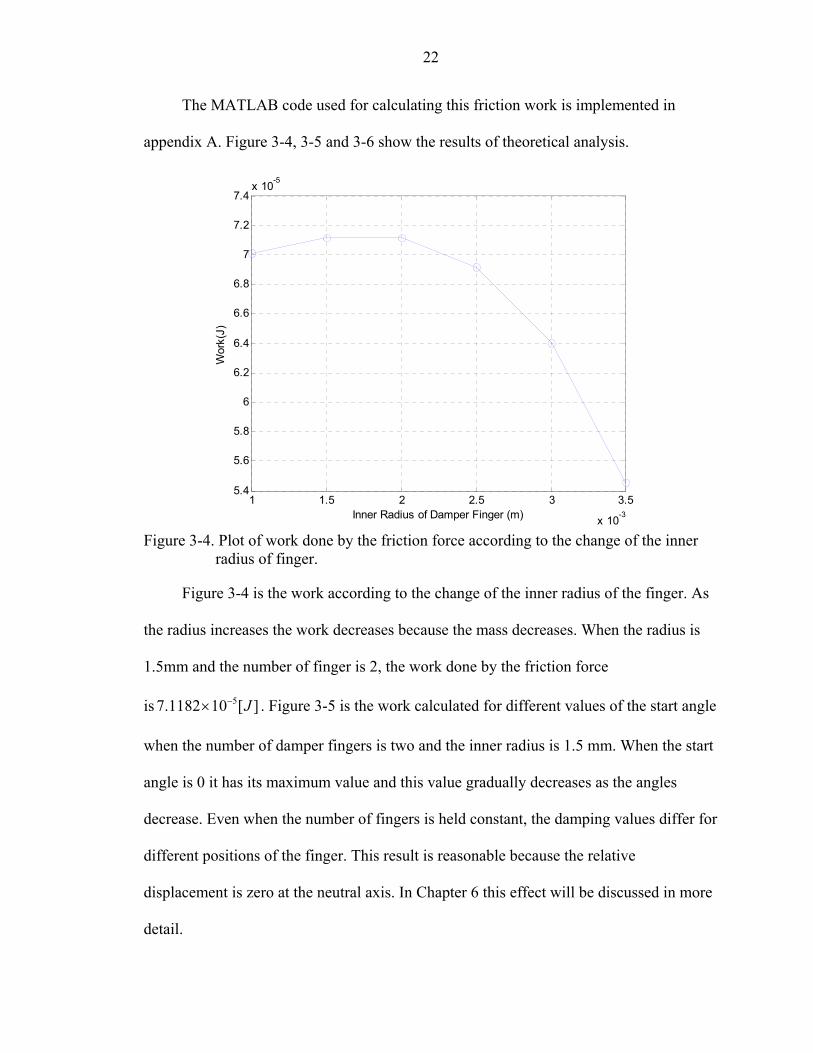
The MATLAB code used for calculating this friction work is implemented in
appendix A. Figure 3-4, 3-5 and 3-6 show the results of theoretical analysis.
1 1.5 2 2.5 3 3.5
x 10-3
5.4
5.6
5.8
6
6.2
6.4
6.6
6.8
7
7.2
7.4x 10⁻⁵
Inner Radius of Damper Finger (m)
Wor
k(J)
Figure 3-4. Plot of work done by the friction force according to the change of the inner
radius of finger.
Figure 3-4 is the work according to the change of the inner radius of the finger. As
the radius increases the work decreases because the mass decreases. When the radius is
1.5mm and the number of finger is 2, the work done by the friction force
is 7.1182 . Figure 3-5 is the work calculated for different values of the start angle
when the number of damper fingers is two and the inner radius is 1.5 mm. When the start
angle is 0 it has its maximum value and this value gradually decreases as the angles
decrease. Even when the number of fingers is held constant, the damping values differ for
different positions of the finger. This result is reasonable because the relative
displacement is zero at the neutral axis. In Chapter 6 this effect will be discussed in more
detail.
510 [ ]J−×

23
0 20 40 60 80 100 120 1400
1
2
3
4
5
6
7
8x 10⁻⁵
Start Angle of Damper Finger (degree)
Wor
k(J)
Figure 3-5. Plot of work done by the friction force for varying start angles of the finger.
The radius of the finger is 1.5 mm and the number of the finger is 2.
0 1 2 3 4 5 6 7 8 9 100
0.2
0.4
0.6
0.8
1
x 10-4
Number of Damper Finger
Wor
k(J)
Figure 3-6. Plot of the work done by the friction force for different numbers of damper
fingers. The inner radius of the finger is 1.5 mm and the start angle is chosen to have the maximum damping in each number of the finger.

24
Figure 3-6 shows the work for different numbers of fingers. The inner radius of the
finger is 1.5 mm and the start angle is chosen to have the maximum damping for the
number of fingers being used. The work increases gradually as the number of fingers is
increased. Finite element analysis will be done for these analytical results in the
following chapter.

CHAPTER 4 BACKGROUND OF FINITE ELEMENTANALYSIS
IN CONTACT PROBLEMS
Since the material properties of the endmill is linear elastic, the classical finite
element can be used without difficulty. Major concern is the contact constraints in the
interface. Contact problems are highly nonlinear and require significant computer
resources to solve for. Contact problems present two significant difficulties. First, the
regions of contact are generally unknown until running the model. Depending on the
loads, material, boundary conditions, and other factors, surfaces can come into and go out
of contact with each other in a largely unpredictable and abrupt manner. Second, most
contact problems need to account for friction. Frictional response can be chaotic, making
solution convergence difficult. In addition to these two difficulties, many contact
problems must also address multi-field effects, such as the conductance of heat and
electrical currents in the areas of contact. In this chapter the general procedure of
performing the contact analysis using FEA is discussed.
Contact problems are characterized by contact constraints which must be imposed
on contacting boundaries. To impose the contact constraints, two basic methods are
available: the Lagrange multiplier method [9] and the penalty method [9]. Other
constraint methods based on the basic methods have been proposed and applied. The
augmented Lagrangian method [9] and the perturbed Lagrangian method [9] are two
examples.
25

26
Contact Formulation in Static Problems
To introduce the basic constraint methods, we consider static mechanical problems
subjected to contact constrains on known contacting boundaries. For small displacements,
the total potential energy of the structure can be written as,
1( )2
Tdd d dS
Ω Ω ΩΠ = Ω− ⋅ Ω− ⋅ −∫ ∫ ∫u e Ce u b u q UT F (4.1)
where Π is the total potential energy of the body, is the engineering strain, is the
elastic modulus, is the body force, is the surface traction. By using standard element
procedures, the discretized form of Eq.(4.1) can be obtained as follows:
e C
b q
1( )2
TΠ = −U U KU UT F
c
(4.2)
where U is the global displacement vector, K is the global stiffness matrix, and F is the
global load vector.
The virtual work due to the contact load is calculated as
(4.3) 1( )
t Ln
cn
W wδ δ=
=∑
where ( ) indicates that the quantity in the parentheses is evaluated in association with a
hitting node n, t is the total number of hitting nodes at time t, and
n
L cwδ the virtual work
due to the concentrated contact force at hitting node n and is calculated as
2 1( )tc iw fδ δ δ t
i= − ⋅u u N (4.4)
where tif is the components of the contact force at a target point in the directions of t .
The virtual displacement
iN
2δu at the target point can be evaluated by using equation
(4.5) 2
1
Nn
nn
δ φ δ=
=∑u 2,u

27
where N denotes the total number of target nodes on the target segment, nφ denotes the
shape function associated with contact node n on the contact segment and is the
displacement of target node n.
2,nuδ
To obtain a matrix expression for 2 1δ δ−u u , the following notation is used:
1 1 1 2,1 2,1 2,1 2, 2, 2,1 2 3 1 2 3 1 2 3...
TN N Nc u u u u u u u u u=u
1 2
1 2
1 2
1 0 0 0 0 0 0 0 0 00 1 0 0 0 0 0 ... 0 00 0 1 0 0 0 0 0 0 0
N
c N
N
φ φ φφ φ φ
φ φ φ
− = − −
Q
Then Eq.(4.4) can be written as
( )tT T t T tc c c i i cw fδ δ δ= =u Q N u rc
where
1 2 3
t Tt t ti i i i
tt T tc c i
N N N
f
=
=
N
r Q N
where t denotes the ijN j th component of the boundary unit vector t . iN
We realize that t is a nodal force vector contributed by the contact at the
associated contacting node. It will be convenient to distinguish, in the evaluation of t ,
between the contribution of normal contact forces and the contribution of tangential
friction forces. Thus we write
cr
cr
t t tc cn= +r r rcf
where
1 1
2,3
tt T tcn c
tt T tcf c J J
f
f summation on J
=
= =
r Q N
r Q N
28
The penetration of the hitting node can be calculated as
( )2 11
t t t tp = − ⋅x x N
where t and t are the position vectors of the hitting node and target point,
respectively.
1x 2x
Expressing t and t in terms of the displacementsu and u , respectively, we
have the following discrete form of the kinematic contact condition:
1x 2x 1 2
( ) ( )2 1 2 1
1
1 0
t t t t t
t Tc c
p
pτ
1= − ⋅ + − ⋅
= + =
x x N u u N
N Q u% (4.6)
where
1
2 1 2 1 2 11 1 2 2 3 3, ,
Tt
T
p
x x x x x x
ττ
τ ττ τ τ τ τ
=
= − − −
N X
X
This means that for small displacements the configuration of the contact system may be
considered unchanged after the displacements. Thus, we can approximate t , by in
Eq.(4.6). Furthermore, we assume only one load step. This means that we need to move
only one step in the “time” domain and
1N% 01N%
pτ and t in Eq.(4.6) can be replaced by and p p0
p , respectively, where denotes any initial penetration (or gap) and p0 p any penetration
after deformation. Therefore, the discretized kinematic contact condition can now be
written as
01 0o T
c cp p= + =N Q u% (4.7)
Eq.(4.7) applies to a single contacting node. If there are contacting nodes,
there will be contact constraint equations, each taking the form of Eq.(4.7). Those
contact constraint equations can be assembled to obtain
)1( >LL
L
L

29
0 0= + =P QU P (4.8)
where
1 2
01
1
00 0 1 2 0
, ,...,
, ,...,
L T
LT
c IITL
p p p
p p p
=
=
=
=
∑
P
Q N Q
p
Since the contacting boundaries are known, all the contacting nodes can be identified and
Eq.(4.8) can be established explicitly.
Based on the above preparations, the contact problem can be stated as follows:
Minimize in Eq.(4.2) subject to the constraints in Eq.(4.8) [P-1] ( )Π U
It must be observed that the mechanical contact condition should be satisfied
automatically by assuming that all the contact nodes are actual contacting nodes. In
general, actual contacting nodes are not known a priori and an iterative trial-and-error
procedure is required to find all contacting nodes. In the following, we discuss the
solution of problem [P-1] with alternative constraint methods.
L
The Lagrange Multiplier Method
In the Lagrange multiplier method, the function to be minimized is replaced by the
following function:
01( , ) ( )2
T T TL∏ = − + +U Λ U KU U F Λ QU P (4.9)
where is an unknown vector which contains as many elements as there are constraint
equations in Eq.(4.8). The elements in are known as Lagrange multipliers.
Λ
Λ

30
The constrained minimization problem [P-1] is now transformed into the following
saddle-point problem:
Find and such that U Λ ( , )L∏ U Λ is stationary, i.e. [P-2]
0
0
L
L
∂∏=
∂∂∏
=∂
U
Λ
(4.10)
Eq.(4.10) yields
0
00
T− + =
+ =
KU F QH ΛQU P
(4.11)
Combining Eq.(4.11), we obtain
L L L=K U F (4.12)
where
0
0
T
L
L
L
=
= −
=
K QK
Q
UF
P
UU
Λ
By solving Eq.(4.12), we can obtain the displacement and the Lagrange multiplier .
The elements in are interpreted as contacting forces at the corresponding contacting
nodes.
U Λ
Λ
The Penalty Method
In the penalty method, the potential energy of the structure is penalized when a
penetration occurs on the contact surface. The following penalty potential is added to the
structural potential:

31
12
Tpπ α= P P
whereα is a diagonal matrix with elements ,iiα which is the penalty parameters and is
a vector of penetration..
P
The function to be minimized is now replaced by
21
2 2
p p
T T 1
πΠ = Π +
= − +U KU U F P αP (4.13)
The constrained minimization problem [P-1] is then transformed into the following
unconstrained minimization problem:
Find such that U pΠ is minimized.
To find its minimum, is held stationary by invoking the following condition: LΠ
0p∂Π=
∂U (4.14)
(4.14)Substituting Eq.(4.13) and (4.8) into , we can obtain
p p=K U F (4.15)
where
0
Tp
TP
= +
= −
K K Q αQ
F F Q α P
The solution of Eq.(4.15) gives the displacement . The contacting forces are then
calculated as
U
C =F αP
where the penetration P is a function of the displacement vector . U

CHAPTER 5 FIITE ELEMENT ANALYSIS
In this chapter, the finite element analysis procedure and results of the endmill
system are presented. Even though the cutting process is dynamic, a static finite element
analysis is performed with the centrifugal force and the cutting force at the tip. Thus, the
friction work obtained must be interpreted as a qualitative measure. Since the simulation
condition is the same as that of the analytical method in Chapter 3, it is still valid to
compare the results of finite element analysis with the analytical results.
Finite Element Model
Figure 5-1. Solid 95, 20 node solid element
The first step of finite element analysis is to build a computational model. The
simplified geometry for the endmill in Chapter 2 is used in the FEA. Using the same
32

33
material properties listed in Table 2-1, 20-node solid elements in ANSYS (solid 95) are
used to build the shank and finger. Figure 5-1 illustrates a 20-node solid element that is
used in ANSYS, and Fig.5-2 plots the finite element model of the endmill with boundary
conditions. In Fig.5-2, the shank is modeled using two elements through the radial
direction, and fingers are modeled inside the shank. The cutting force F=100N is
distributed to 4 nodes at the tip. Table5-1 shows the number of elements used in the
endmill finite element model.
Figure 5-2. FEA model of the endmill using 20 node cubic elements and 8 node contact elements with boundary conditions.
Table 5-1. The number of nodes and elements. Node 24826
Element 6480 SOLID95 4320
TARGE170 1080 CONTA174 1080

34
Because the contact area is curved, higher order elements must be used to prevent
inaccurate representation of the surface. Since the contact element is defined on the
surface of solid elements, the consistent order of the element must be used for the
structure and contact surface. The counter part of SOLID95 structural element is 8-node
contact element, as illustrated in Fig.5-3. The contact elements are defined between the
shank and finger.
Figure 5-3. 8-node contact (CONTA174) and target (TARGE170) element description.
ANSYS offers CONTA174 and TARGE170 for contact and target elements,
respectively. CONTA174 is used to represent the contact and sliding between 3-D
“target” surfaces and a deformable surface, defined by this element. The element is
applicable to 3-D structural and coupled thermal-structural contact analysis. This element
is located on the surfaces of 3-D solid or shell elements with midside nodes. It has the
same geometric characteristics as the solid or shell element face with which it is
connected. Contact occurs when the element surface penetrates one of the target segment
elements on a specified target surface. Coulomb and shear stress friction is allowed.

35
TARGE170 is used to represent various 3-D target surfaces for the associated
contact elements. The contact elements themselves overlay the solid elements describing
the boundary of a deformable body and are potentially in contact with the target surface,
defined by TARGE170. This target surface is discretized by a set of target segment
elements (TARGE170) and is paired with its associated contact surface via a shared real
constant set. Any translational or rotational displacement, temperature, and voltage on the
target segment element can be imposed. Forces and moments on target elements can also
be imposed.
Boundary Conditions
According to the forces applied to the endmill, we can divide the analysis
procedure into two steps. The first step is when the endmill starts rotating. In this step,
only the angular velocity of 2,722.713 [ is applied without considering the
cutting force.
/ sec]rad
Force
Vertical Force =100 [N]
Rotational Velocity=2722.713 [rad/s]
Time Step 1 Time Step 2 Time (sec)
Figure 5-4. Force boundary conditions in each time step. Each time step is divided into 5 steps.

36
The second step is when the endmill starts the cutting process. At this time a
vertical force of 100 N is applied at the tip of the endmill. Figure 5-4 illustrates the force
boundary conditions in each step. Each time step is divided into 5 substeps in order to
improve the convergence of nonlinear analysis.
Calculation of Friction Work
Even if the structure is linear elastic, the contact constraints make the problem
nonlinear. In ANSYS, a Newton-Raphson iterative method is employed to solve the
nonlinear system of equations. All default parameters in ANSYS are used in nonlinear
analysis.
Figure 5-5. Diagram explaining how to
After finishing FEA, the dampin
calculated. The input commands to AN
Appendix D. Figure 5-5 shows a schem
stress and the relative slide in each con
assuming a constant stress within an el
Friction Stress
(Relativcalculate the damping work.
g work which is done by the f
SYS for obtaining the frictio
atic procedure of the calcula
tact element are obtained for
ement, the friction force can b
Slide
e Displacement)
Damping = Dot Product of Friction Force and Slide (Relative Displacement)
Contact Surface
riction force is
nal work are listed in
tion. First, the friction
each load step. By
e obtained by

37
multiplying the friction stress with the element area. The dot product of the friction force
vector and the relative displacement vector in each substep and in each element yields the
friction work.
Finite Element Analysis Results
Load Step 1
Figure 5-6 is the results at load step 1 when only the angular velocity is applied. In
Chapter 3, the analytical method estimates the contact pressure to be 0.27[ ]MPa .
)
Figure 5-6. FEA result for loadvon misses stress (Mstress (MPa), and (dvalue and MN mea
(a)
step 1 when only the angular velocity is appliPa), (b) is the contact pressure (MPa), (c) is th
) is the slide (mm). MX indicates where the mns the minimum value.
(b
)
(c) (ded. (a) is the e frictional
aximum

38
Whereas, the maximum contact pressure from FEA is 0.58[ ]MPa , as shown in
Fig.5-6 (b). Since the actual contact occurs only half of the contact surface, the higher
contact pressure from FEA is expected. In addition, the contact pressure is not constant:
maximum at the top and the bottom surface and zero at both sides. Even though we
assume that there is no relative motion between the contact surfaces during load step 1 in
Chapter 3, there is a relative motion due to the diameter change. However, the relative
motion in load step 1 should not be counted because it is not related to the chatter
vibration.
Load Step 2 (Centrifugal Force + Vertical Force)
In the load step 2, a vertical force (cutting force) is applied on top of the centrifugal
force. Figure 5-7 shows the results of load step 2. The frictional work is calculated by dot
producing the friction force (Fig.5-7 (c)) and the relative slide (Fig.5-7 (d)). Since the
load step is divided into five sub steps, the friction work at each sub step must be
summed. The total friction work during load step 2 is 3.3426 . By comparing
with the analytical results in Chapter 3, the finite element analysis
estimates about 50% of the analytical result. The friction work calculated from FEA is
less than that from the analytical approach because the actual contact area is small in
FEA. There is no contact on two sides: the neutral axis lies and the fixed end. In addition,
the contact pressure is not constant. That is why the analytical result is about two times
higher than the FEA result. Another interesting observation is that most of the relative
displacement occurs on the bottom side of the finger (see Fig.5-7 (d)). That happens
because the vertical force is applied to the top side of the endmill.
510 [ ]J−×
57.1182 10 [ ]J−×

39
)
)
Figure 5-7. FEA result for load sapplied. (a) is the von(c) is the frictional stwhere the maximum
Figure 5-8, a schematic dia
explains in more detail. This figu
Fig.5-8 (a) shows the initial state
is applied and the deformed shap
the length of the shank reduces a
finger is not reduced because the
vertical load is applied on top of
deformed, as illustrated in Fig.5-
deflected shape has the largest sl
(c)
tep 2 when both ngular velocity and vertical misses stress (MPa), (b) is the contact press
ress (MPa), and (d) is the slide (mm). MX indvalue and MN means the minimum value.
gram of endmill bending according to the ap
re is exaggerated; the real deformation is ver
. When the endmill starts rotating, the centrif
e looks like Fig.5-8 (b). Due to the mass con
s the diameter increases. Whereas, the length
cylindrical finger is cut along its neutral axi
the centrifugal force, the shank and the finge
8 (c). Due to the difference in geometric cen
ide at the bottom surface.
(d
(a)
(bforce are ure (MPa), icates
plied force,
y small.
ugal force
servation,
of the
s. When the
r are
ter, the

40
(a)
(b)
(c)
Figure 5-8.Schematic diagram of endmill behavior according to the applied forces. (a) shows the initial state, in (b) the angular velocity is applied and in (c) the vertical force is added.

CHAPTER 6 PARAMETER STUDY
In this chapter, a parameter study is performed to find the maximum value of the
damping work. Two design variables, the inner radius of the finger and the number of the
fingers, are changed. The results of the parameter study are discussed with respect to the
results of the analytical approach.
Determination of the Mesh Size
It is very important to determine the proper mesh size. A fine mesh will usually
give an accurate result, but it requires a large amount of computational cost. Since the
finite element analysis needs to be repeated 45 times during the parameter study,
computational cost is an important issue.
0 0.2 0.4 0.6 0.8 1 1.2 1.4 1.6 1.8 2
x 104
3.15
3.2
3.25
3.3
3.35x 10⁻⁵
Element Number
Wor
k(J)
Figure 6-1. Damping according to the number of elements. Number of fingers = 2, inner radius R1=1mm, and start angle α = 0.
41

42
Figure 6-1 shows the damping work according to the change of the number of
elements. The work gradually increases until the element number reaches 4200, and then
it converges on 3.28 . Based on these results the number of elements is chosen
to be 4200.
510 [ ]J−×
Determination of the Start Angle.
Before starting the parameter study, a start angle must be chosen for different
configurations. This is because the damping value changes with starting angle even if the
same number of fingers is used.
5
03.28 10 [ ]
Start AngleWork J−
=
= ×
o
5
452.01 10 [ ]
Start AngleWork J−
=
= ×
o
5
900.95 10 [ ]
Start AngleWork J−
=
= ×
o
5
1352.01 10 [ ]
Start AngleWork J−
=
= ×
o
5
02.86 10 [ ]
Start AngleWork J−
=
= ×
o
5
03.40 10 [ ]
Start AngleWork J−
=
= ×
o
5
302.16 10 [ ]
Start AngleWork J−
=
= ×
o
5
602.86 10 [ ]
Start AngleWork J−
=
= ×
o
5
903.41 10 [ ]
Start AngleWork J−
=
= ×
o
5
182.82 10 [ ]
Start AngleWork J−
=
= ×
o
5
363.40 10 [ ]
Start AngleWork J−
=
= ×
o
5
543.70 10 [ ]
Start AngleWork J−
=
= ×
o
Figure 6-2. Damping according to the position of the finger
43
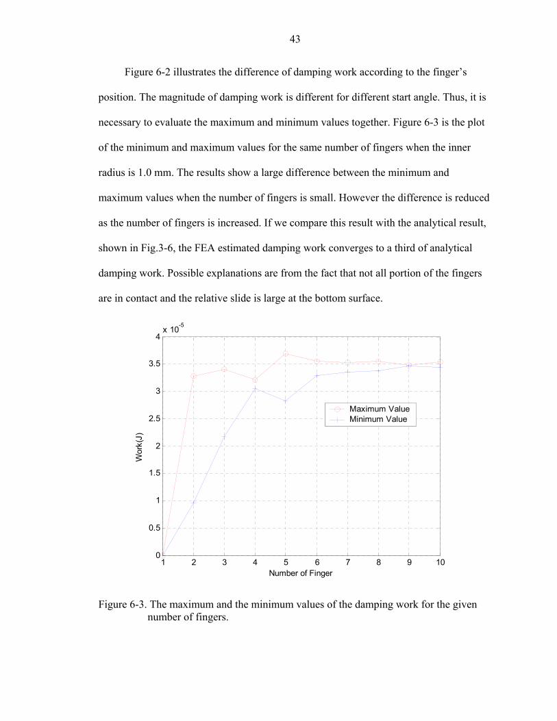
Figure 6-2 illustrates the difference of damping work according to the finger’s
position. The magnitude of damping work is different for different start angle. Thus, it is
necessary to evaluate the maximum and minimum values together. Figure 6-3 is the plot
of the minimum and maximum values for the same number of fingers when the inner
radius is 1.0 mm. The results show a large difference between the minimum and
maximum values when the number of fingers is small. However the difference is reduced
as the number of fingers is increased. If we compare this result with the analytical result,
shown in Fig.3-6, the FEA estimated damping work converges to a third of analytical
damping work. Possible explanations are from the fact that not all portion of the fingers
are in contact and the relative slide is large at the bottom surface.
1 2 3 4 5 6 7 8 9 100
0.5
1
1.5
2
2.5
3
3.5
4x 10⁻⁵
Number of Finger
Wor
k(J)
Maximum ValueMinimum Value
Figure 6-3. The maximum and the minimum values of the damping work for the given number of fingers.
44
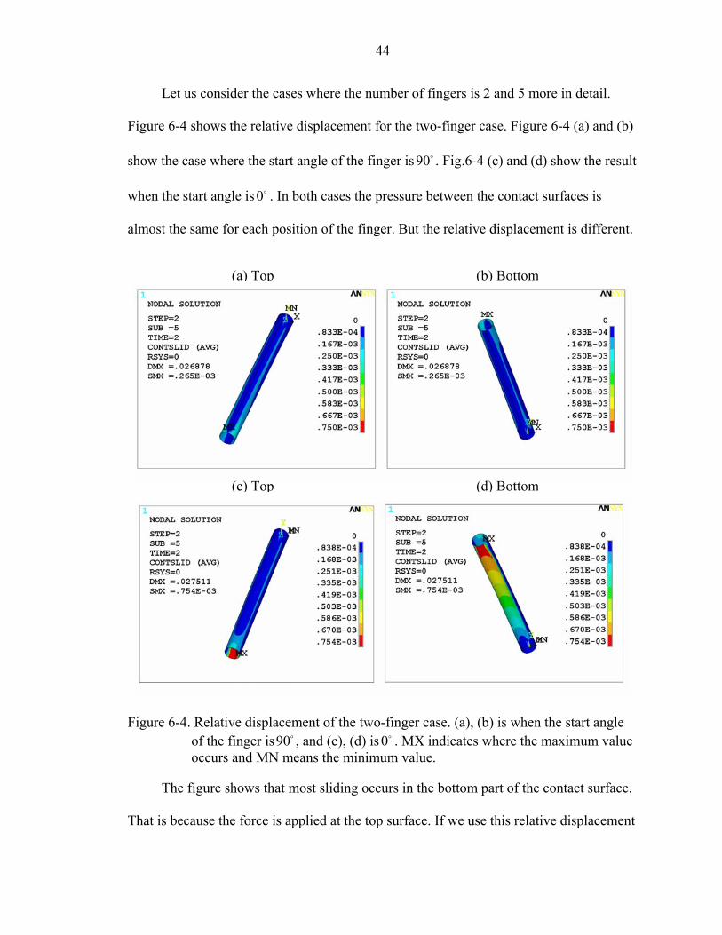
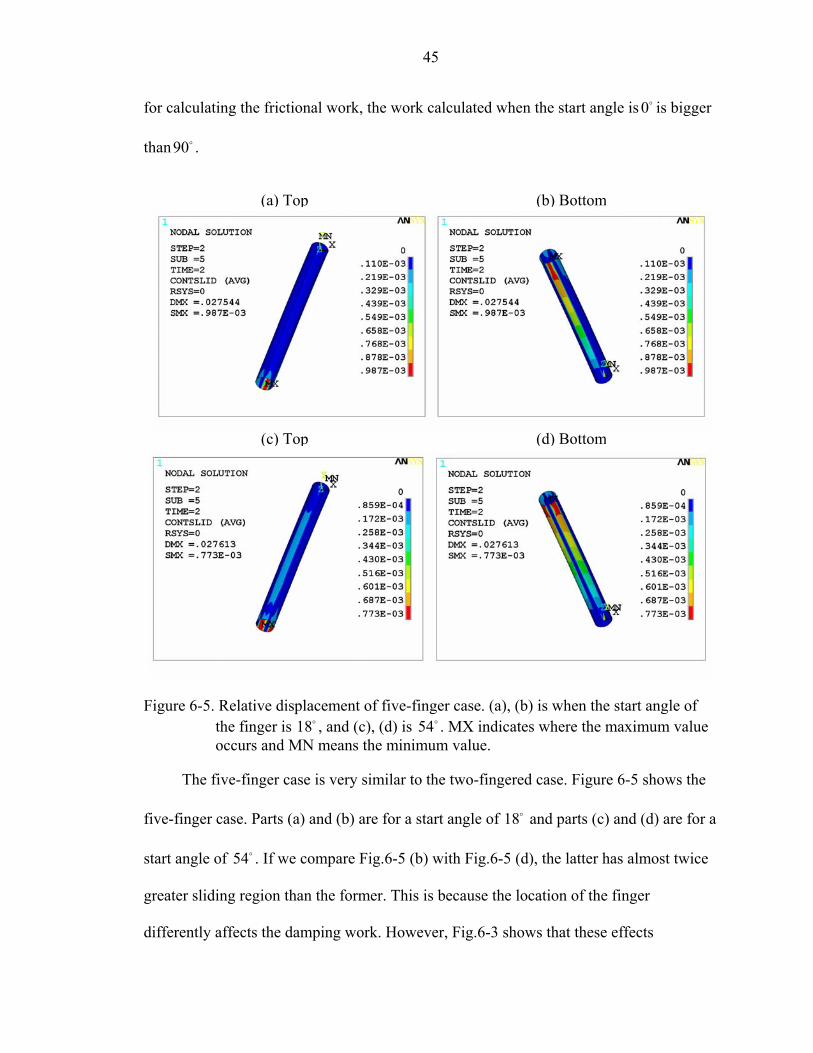
Let us consider the cases where the number of fingers is 2 and 5 more in detail.
Figure 6-4 shows the relative displacement for the two-finger case. Figure 6-4 (a) and (b)
show the case where the start angle of the finger is . Fig.6-4 (c) and (d) show the result
when the start angle is 0 . In both cases the pressure between the contact surfaces is
almost the same for each position of the finger. But the relative displacement is different.
90o
o
Figure 6-4. Relatiof the occurs
The figure
That is because th
(a) Top
ve displacement of the two-finger case. (a)finger is90 , and (c), (d) is 0 . MX indicate and MN means the minimum value.
o o
shows that most sliding occurs in the bottom
e force is applied at the top surface. If we u
(b) Bottom
(c) Top (d) Bottom, (b) is when the start angle s where the maximum value
part of the contact surface.
se this relative displacement
45
for calculating the frictional work, the work calculated when the start angle is 0 is bigger
than .
o
90o
Figure 6-5. Relatithe finoccurs
The five-fin
five-finger case. P
start angle of
greater sliding reg
differently affects
54o
(a) Top
ve displacement of five-finger case. (a), (b)ger is 18 , and (c), (d) is . MX indicate and MN means the minimum value.
o 54o
ger case is very similar to the two-fingered
arts (a) and (b) are for a start angle of 18
. If we compare Fig.6-5 (b) with Fig.6-5 (d
ion than the former. This is because the loc
the damping work. However, Fig.6-3 show
o
(b) Bottom
(c) Top (d) Bottomis when the start angle of s where the maximum value
case. Figure 6-5 shows the
and parts (c) and (d) are for a
), the latter has almost twice
ation of the finger
s that these effects
46
disappear as the number of fingers increases. This means that when the number of fingers
is small the work done by the friction force depends on the start angle.
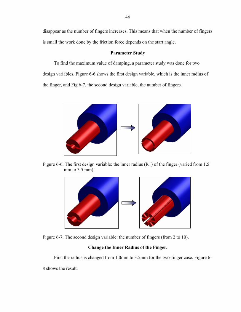
Parameter Study
To find the maximum value of damping, a parameter study was done for two
design variables. Figure 6-6 shows the first design variable, which is the inner radius of
the finger, and Fig.6-7, the second design variable, the number of fingers.
Figure 6-6. The first design variable: the inner radius (R1) of the finger (varied from 1.5 mm to 3.5 mm).
Figure 6-7. The second design variable: the number of fingers (from 2 to 10).
Change the Inner Radius of the Finger.
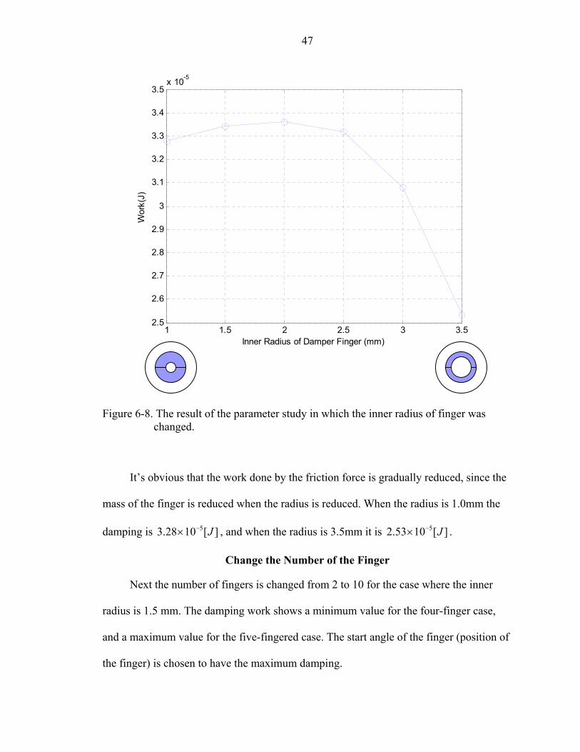
First the radius is changed from 1.0mm to 3.5mm for the two-finger case. Figure 6-
8 shows the result.
47
1 1.5 2 2.5 3 3.52.5
2.6
2.7
2.8
2.9
3
3.1
3.2
3.3
3.4
3.5x 10⁻⁵
Inner Radius of Damper Finger (mm)
Wor
k(J)
Figure 6-8. The result of the parameter study in which the inner radius of finger was changed.
It’s obvious that the work done by the friction force is gradually reduced, since the
mass of the finger is reduced when the radius is reduced. When the radius is 1.0mm the
damping is , and when the radius is 3.5mm it is .
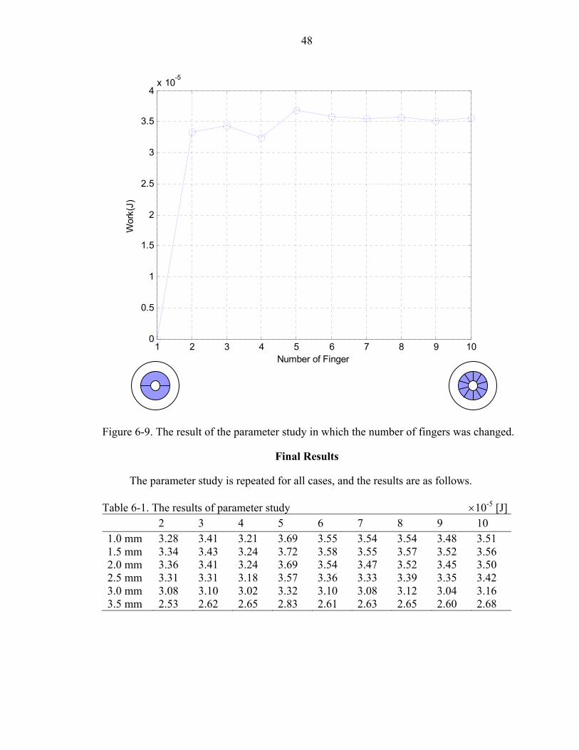
Change the Number of the Finger
Next the number of fingers is changed from 2 to 10 for the case where the inner
radius is 1.5 mm. The damping work shows a minimum value for the four-finger case,
and a maximum value for the five-fingered case. The start angle of the finger (position of
the finger) is chosen to have the maximum damping.
53.28 10 [ ]J−× 52.53 10 [ ]J−×
48
1 2 3 4 5 6 7 8 9 100
0.5
1
1.5
2
2.5
3
3.5
4x 10⁻⁵
Number of Finger
Wor
k(J)
Figure 6-9. The result of the parameter study in which the number of fingers was changed.
Final Results
The parameter study is repeated for all cases, and the results are as follows.
Table 6-1. The results of parameter study ×10-5 [J] 2 3 4 5 6 7 8 9 10 1.0 mm 3.28 3.41 3.21 3.69 3.55 3.54 3.54 3.48 3.51 1.5 mm 3.34 3.43 3.24 3.72 3.58 3.55 3.57 3.52 3.56 2.0 mm 3.36 3.41 3.24 3.69 3.54 3.47 3.52 3.45 3.50 2.5 mm 3.31 3.31 3.18 3.57 3.36 3.33 3.39 3.35 3.42 3.0 mm 3.08 3.10 3.02 3.32 3.10 3.08 3.12 3.04 3.16 3.5 mm 2.53 2.62 2.65 2.83 2.61 2.63 2.65 2.60 2.68
49
11.5
22.5
33.5
23
45
67
89
10
2
2.5
3
3.5
4
x 10-5
Inner Radius of Damper Finger (mm)Number of Finger
Wor
k(J)
Figure 6-10. The plot of the Table 6-1.
In order to find the configuration that yields the maximum damping work, the first
design variable (R1) is changed by six different values and the second design variable
(number of finger) is changed by nine different values. Table 6-1 shows the results in 6×9
matrix. In each configuration, the start angle is chosen such that the maximum damping
work can be occurred. Figure 6-10 plots the response surface of the damping work. Even
if the second design variable is discrete, a continuous surface is plotted for illustration
purpose. It is noted that the local peak when the number of fingers is five is maintained
throughout all different radii. The general trend of the response surface is consistent.
Based on the response surface, we can conclude that the damping work has its maximum
value when the inner radius is 1.5 mm and the number of fingers is 5. However, the large
50
difference in maximum and minimum damping values in this configuration, as shown in
Fig.6-3, may reduce the significance of this choice of design.
As a conclusion, the effect of damping work increases as the number of fingers is
increased and the inner radius is decreased.
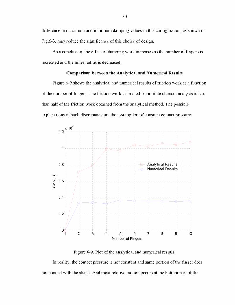
Comparison between the Analytical and Numerical Results
Figure 6-9 shows the analytical and numerical results of friction work as a function
of the number of fingers. The friction work estimated from finite element analysis is less
than half of the friction work obtained from the analytical method. The possible
explanations of such discrepancy are the assumption of constant contact pressure.
1 2 3 4 5 6 7 8 9 100
0.2
0.4
0.6
0.8
1
1.2x 10⁻⁴
Number of Fingers
Wor
k(J)
Analytical ResultsNumerical Results
Figure 6-9. Plot of the analytical and numerical resutls.
In reality, the contact pressure is not constant and same portion of the finger does
not contact with the shank. And most relative motion occurs at the bottom part of the

51
endmill. That is because the vertical force is applied at the top and the nonlinearity
associated with the centrifugal force contributes the asymmetry between the top and
bottom fingers. During the nonlinear analysis ANSYS automatically update the geometry
and refer to the deformed configuration, which means the body force is calculated at the
deformed geometry. Even though the analytical and numerical results show the
difference, the general trends of both results are very similar each other.
In order to explain the general trends of friction work, consider the analytical
explanation of the contact pressure:
2
cc
MRPAω
= ,
wherec
MA
andω is constant. Value R , which is the distance between the rotational center
and the mass center of the finger, can be calculated by
( )( )
3 32 1
2 22 1
2 sin( )3
R RR
R Rα
α
−=
−
If we assume that the friction work is proportional to the contact pressure, then the
friction work is proportional to R , which increases as the number of fingers increases. If
the number of the finger increases, which means the angleα goes to zero, R is converges
to
( )( )
3 32 1
2 22 1
2
3
R RR
R R
−=
−
Therefore, the maximum value of the contact pressure can be calculated by
( )( )
3 32 22 1
2 22 1
2
3cc c
R RMR MPA AR Rω ω−
= =−

52
As a conclusion, the friction work increases along with the number of fingers, but
its effect is reduced as the number of fingers increases.

CHAPTER 7 CONCLUSION AND FUTURE WORK
The goal of this research was to design the mechanical damper which is inserted
into the endmill. Through the nonlinear finite element analysis and parameter study, the
trend of the damping effect is identified.
The results from the analytical method were used to verify the FEA result.
Although the number and the inner radius of finger were varied in finite element analysis,
only the two-finger case was considered in the comparison. The FEA results were smaller
than those of the analytical approach because some regions did not contact and the
contact pressure was not constant.
A parameter study was carried out by changing the inner radius and the number of
fingers. The inner radius was varied from 1.0 mm to 3.5 mm, and the number of fingers
was varied from 2 to 10. The results show general trends of the damping work according
to the change of the two design variables. As the inner radius decreased and the number
of finger increased, the damping work increased. The Maximum value was
when the inner radius was 1.5 mm and the number of fingers was 5. The parameter study
also showed that when the number of the fingers is small the damping work is affected by
the position of the finger, but that this dependence disappears as the number of finger
increases.
53.72 10 [ ]J−×
Recommendations for Future Research
As discussed in Chapter 6, the damping work depends on the start angle. However,
in practice the endmill is continuously rotating. Thus, it is recommended to perform a
53

54
series of static FEA by rotating the endmill by on cycle and to calculate the integrated
damping work. This procedure will provide more accurate estimation of the real damping
work.

APPENDIX A MATLAB CODE FOR THEORITICAL ANALYSIS
%------------------------------------------------------------------------------------- % Matlab function to calculate the work done by the friction force % % By Dongki Won %------------------------------------------------------------------------------------- function cal_work %------------------------------------------------------------------------------------- % Material Properties, radius and applied forces. %------------------------------------------------------------------------------------- E=2.0678e11; %- Modulus of Elasticity : 2.0*10^11[MPa] rho=7820; %- Mass Density : 7820[kg/m^3] mu=0.15; %- Friction Coefficient : 0.15 r1=1.5e-3; r2=4.7625e-3; r3=r2; r4=9.525e-3; L=101.6e-3; omega=2722; F=100; %------------------------------------------------------------------------------------- % Calculate the work according to the chage of the inner raius of finger. %------------------------------------------------------------------------------------- n=2;m=1; for r1=1.0e-3:0.5e-3:3.5e-3 ang(1)=0; for i=1:n ang(i+1)=ang(1)+(360/n)*i; end ang=ang*(pi/180); II=(1/4)*((r4)^4-(r3)^4)*pi; for i=1:(n-1) tmp1=sin(ang(i+1))*cos(ang(i+1))-sin(ang(i))*cos(ang(i))-(ang(i+1)-ang(i)); tmp1=tmp1*((r1)^4-(r2)^4); tmp1=tmp1*(1/8); II=II+tmp1; end work=0; for i=1:n alpha=(ang(i+1)-ang(i))/2;
55

56
d1=(2*sin(alpha).*(r2^3-r1^3))/(3*alpha*(r2^2-r1^2)); d2=d1*sin((ang(i)+ang(i+1))*0.5); V=(ang(i+1)-ang(i))*(r2^2-r1^2)*L*0.5; P=abs(V*rho*(omega^2)*d1/L); work=work+abs((1/3)*(L^3)*mu*P*F*d2/(E*II)); end y1(m)=work; m=m+1; end x1=[1.0e-3:0.5e-3:3.5e-3]; plot(x1,y1,'b-o'); grid; xlabel('Inner Radius of Damper Finger (m)'); ylabel('Work(J)'); [tmp,n]=size(x1); clc fprintf('\nCalculate the work according to the chage of the inner raius of finger.\n'); fprintf('The Number of Finger=%3.0f\nStart Angle=%3.0f [Degree]\n',n,0); for i=1:n fprintf('Inner Raius of Finger =%16.9e [m]\t\tWork=%16.9e [J]\n',x1(i),y1(i)); end %------------------------------------------------------------------------------------- % Calculate the work according to the chage of the start angle of finger. %------------------------------------------------------------------------------------- n=2;m=1;r1=1.5e-3; atmp=(360/n)/4; for a=0:atmp:atmp*3 ang(1)=a; for i=1:n ang(i+1)=ang(1)+(360/n)*i; end ang=ang*(pi/180); II=(1/4)*((r4)^4-(r3)^4)*pi; for i=1:(n-1) tmp1=sin(ang(i+1))*cos(ang(i+1))-sin(ang(i))*cos(ang(i))-(ang(i+1)-ang(i)); tmp1=tmp1*((r1)^4-(r2)^4); tmp1=tmp1*(1/8); II=II+tmp1; end work=0; for i=1:n alpha=(ang(i+1)-ang(i))/2; d1=(2*sin(alpha).*(r2^3-r1^3))/(3*alpha*(r2^2-r1^2)); d2=d1*sin((ang(i)+ang(i+1))*0.5); V=(ang(i+1)-ang(i))*(r2^2-r1^2)*L*0.5; P=abs(V*rho*(omega^2)*d1/L);

57
work=work+abs((1/3)*(L^3)*mu*P*F*d2/(E*II)); end y2(m)=work; m=m+1; end x2=[0:atmp:atmp*3]; figure; plot(x2,y2,'b-o'); grid; xlabel('Start Angle of Damper Finger (degree)'); ylabel('Work(J)'); [tmp,n]=size(x2); fprintf('\nCalculate the work according to the chage of the start angle of finger.\n'); fprintf('Number of Finger=%5.0f\nInner Radius of the Finger=%16.9e [m]\n',2,r1); for i=1:n fprintf('Start Angle =%16.9e [Degree]\t\tWork=%16.9e [J]\n',x2(i),y2(i)); end %------------------------------------------------------------------------------------- % Calculate the work according to the change of the number of finger. %------------------------------------------------------------------------------------- m=1;clear ang for n=2:10 clear ang atmp=(1+(-1)^(n-1))/2; ang(1)=((360/n)/4)*atmp; for i=1:n ang(i+1)=ang(1)+(360/n)*i; end ang=ang*(pi/180); II=(1/4)*((r4)^4-(r3)^4)*pi; for i=1:(n-1) tmp1=sin(ang(i+1))*cos(ang(i+1))-sin(ang(i))*cos(ang(i))-(ang(i+1)-ang(i)); tmp1=tmp1*((r1)^4-(r2)^4); tmp1=tmp1*(1/8); II=II+tmp1; end work=0; for i=1:n alpha=(ang(i+1)-ang(i))/2; d1=(2*sin(alpha).*(r2^3-r1^3))/(3*alpha*(r2^2-r1^2)); d2=d1*sin((ang(i)+ang(i+1))*0.5); V=(ang(i+1)-ang(i))*(r2^2-r1^2)*L*0.5; P=abs(V*rho*(omega^2)*d1/L); work=work+abs((1/3)*(L^3)*mu*P*F*d2/(E*II)); end y3(m+1)=work;

58
m=m+1; end x3=[1:10]; figure; plot(x3,y3,'b-o'); axis([0,10,0,11e-5]); grid; xlabel('Number of Damper Finger'); ylabel('Work(J)'); [tmp,n]=size(x3); fprintf('\nCalculate the work according to the chage of the number of finger.\n'); fprintf('Inner Radius of the Finger=%16.9e [m]\n',r1); for i=1:n fprintf('Number of Finger =%3.0f\t\tWork=%16.9e [J]\n',x3(i),y3(i)); end
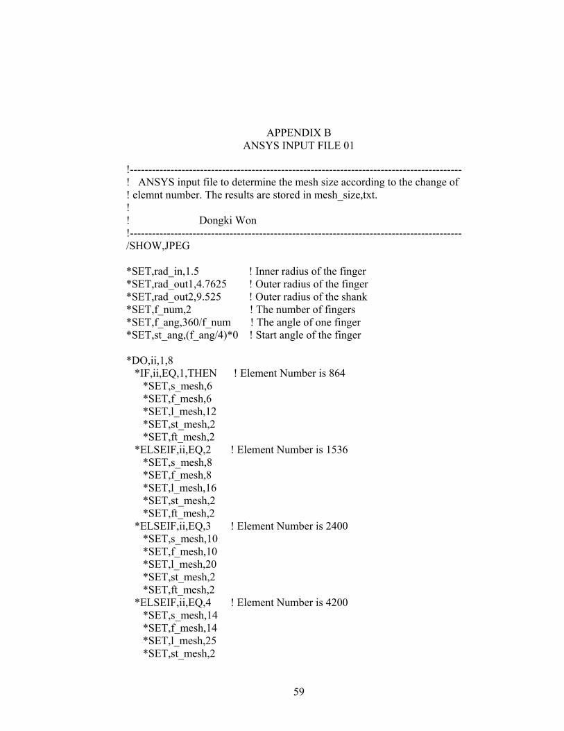
APPENDIX B ANSYS INPUT FILE 01
!------------------------------------------------------------------------------------------ ! ANSYS input file to determine the mesh size according to the change of ! elemnt number. The results are stored in mesh_size,txt. ! ! Dongki Won !------------------------------------------------------------------------------------------ /SHOW,JPEG *SET,rad_in,1.5 ! Inner radius of the finger *SET,rad_out1,4.7625 ! Outer radius of the finger *SET,rad_out2,9.525 ! Outer radius of the shank *SET,f_num,2 ! The number of fingers *SET,f_ang,360/f_num ! The angle of one finger *SET,st_ang,(f_ang/4)*0 ! Start angle of the finger *DO,ii,1,8 *IF,ii,EQ,1,THEN ! Element Number is 864 *SET,s_mesh,6 *SET,f_mesh,6 *SET,l_mesh,12 *SET,st_mesh,2 *SET,ft_mesh,2 *ELSEIF,ii,EQ,2 ! Element Number is 1536 *SET,s_mesh,8 *SET,f_mesh,8 *SET,l_mesh,16 *SET,st_mesh,2 *SET,ft_mesh,2 *ELSEIF,ii,EQ,3 ! Element Number is 2400 *SET,s_mesh,10 *SET,f_mesh,10 *SET,l_mesh,20 *SET,st_mesh,2 *SET,ft_mesh,2 *ELSEIF,ii,EQ,4 ! Element Number is 4200 *SET,s_mesh,14 *SET,f_mesh,14 *SET,l_mesh,25 *SET,st_mesh,2
59

60
*SET,ft_mesh,2 *ELSEIF,ii,EQ,5 ! Element Number is 6480 *SET,s_mesh,18 *SET,f_mesh,18 *SET,l_mesh,30 *SET,st_mesh,2 *SET,ft_mesh,2 *ELSEIF,ii,EQ,6 ! Element Number is 8640 *SET,s_mesh,18 *SET,f_mesh,18 *SET,l_mesh,30 *SET,st_mesh,3 *SET,ft_mesh,3 *ELSEIF,ii,EQ,7 ! Element Number is 11500 *SET,s_mesh,18 *SET,f_mesh,18 *SET,l_mesh,40 *SET,st_mesh,3 *SET,ft_mesh,3 *ELSEIF,ii,EQ,8 ! Element Number is 19200 *SET,s_mesh,20 *SET,f_mesh,20 *SET,l_mesh,60 *SET,st_mesh,3 *SET,ft_mesh,3 *ENDIF tmp1=s_mesh*l_mesh*2*(1+st_mesh) tmp2=f_mesh*l_mesh*2*(1+ft_mesh) num_elem=tmp1+tmp2 /INPUT,endmill_model,inp /INPUT,endmill_work,inp /OUTPUT,mesh_size,txt,,APPEND *VWRITE,num_elem,work (F7.0,3X,F16.9,3X) /OUTPUT *ENDDO

APPENDIX C ANSYS INPUT FILE 02
!------------------------------------------------------------------------------------------ ! ANSYS input file to determine the start angle of the finger. ! The results are stored in start_angle,txt. ! ! Dongki Won !------------------------------------------------------------------------------------------ /SHOW,JPEG *SET,rad_in,1 ! Inner radius of the finger *SET,rad_out1,4.7625 ! Outer radius of the finger *SET,rad_out2,9.525 ! Outer radius of the shank *SET,s_mesh,14 *SET,l_mesh,30 *SET,st_mesh,2 *SET,ft_mesh,2 *DO,ii,8,10 *SET,f_num,ii *SET,f_ang,360/f_num *IF,ii,EQ,2,THEN *SET,f_mesh,14 *ELSEIF,ii,EQ,3 *SET,f_mesh,9 *ELSEIF,ii,EQ,4 *SET,f_mesh,7 *ELSEIF,ii,EQ,5 *SET,f_mesh,6 *ELSEIF,ii,EQ,6 *SET,f_mesh,5 *ELSEIF,ii,EQ,7 *SET,f_mesh,4 *ELSEIF,ii,EQ,8 *SET,f_mesh,4 *SET,s_mesh,16 *SET,ft_mesh,2 *ELSEIF,ii,EQ,9 *SET,f_mesh,4 *SET,s_mesh,18 !*SET,ft_mesh,2
61

62
*ELSEIF,ii,EQ,10 *SET,f_mesh,3 *SET,s_mesh,15 !*SET,ft_mesh,3 *ENDIF *DO,jj,0,3 *SET,st_ang,(f_ang/4)*jj /INPUT,endmill_model,inp /INPUT,endmill_work,inp /OUTPUT,start_angle,txt,,APPEND *VWRITE,f_num,jj,st_ang,work (F7.0,3X,F7.0,3X,F16.9,3X,F16.9,3X) /OUTPUT *ENDDO *ENDDO

APPENDIX D ANSYS INPUT FILE 03
!------------------------------------------------------------------------------------------ ! ANSYS input file to do the parameter study as the change of two design ! variables, the number of the finger(f_num) and the inner radius of the finger ! (rad_in). The results are stored in parameter_study,txt. ! ! Dongki Won !------------------------------------------------------------------------------------------ /SHOW,JPEG *SET,rad_out1,4.7625 ! Outer radius of the finger *SET,rad_out2,9.525 ! Outer radius of the shank *SET,s_mesh,14 *SET,l_mesh,25 *SET,st_mesh,2 *SET,ft_mesh,2 *DO,ii,2,10 *SET,f_num,ii *SET,f_ang,360/f_num *IF,ii,EQ,2,THEN *SET,f_mesh,14 *SET,st_ang,(f_ang/4)*0 *ELSEIF,ii,EQ,3 *SET,f_mesh,9 *SET,st_ang,(f_ang/4)*3 *ELSEIF,ii,EQ,4 *SET,f_mesh,7 *SET,st_ang,(f_ang/4)*2 *ELSEIF,ii,EQ,5 *SET,f_mesh,6 *SET,st_ang,(f_ang/4)*3 *ELSEIF,ii,EQ,6 *SET,f_mesh,5 *SET,st_ang,(f_ang/4)*2 *ELSEIF,ii,EQ,7 *SET,f_mesh,4 *SET,st_ang,(f_ang/4)*3 *ELSEIF,ii,EQ,8 *SET,f_mesh,4
63

64
*SET,s_mesh,16 *SET,st_ang,(f_ang/4)*2 *ELSEIF,ii,EQ,9 *SET,f_mesh,4 *SET,s_mesh,18 *SET,st_ang,(f_ang/4)*3 *SET,ft_mesh,2 *SET,l_mesh,30 *ELSEIF,ii,EQ,10 *SET,f_mesh,3 *SET,s_mesh,15 *SET,st_ang,(f_ang/4)*2 *SET,ft_mesh,2 *SET,l_mesh,25 *ENDIF *DO,jj,1,3.5,0.5 *SET,rad_in,jj /INPUT,endmill_model,inp /INPUT,endmill_work,inp /OUTPUT,parameter_study,txt,,APPEND *VWRITE,f_num,rad_in,work (F7.0,3X,F16.9,3X,F16.9,3X) /OUTPUT *ENDDO *ENDDO

APPENDIX E ANSYS INPUT FILE 04
!------------------------------------------------------------------------------------------ ! ANSYS input file to solve the endmill model. This input file is used ! in endmill_run.inp and endmill_start.inp ! ! Dongki Won !------------------------------------------------------------------------------------------ PARSAV /CLEAR PARRES /FILNAME,endmill,1 /UNITS,MPA /TITLE,Damping Design of Endmill /prep7 !--------------------------------------------------------------------- ! Element Type and Material Properties !--------------------------------------------------------------------- ET,1,SOLID95 !- 20-Nodes Cubic Element MP,EX,1,206800 !- Modulus of Elasticity : 206780[MPa] MP,DENS,1,7.82e-9 !- Mass Density : 7.82e-6[kg/mm^3] MP,NUXY,1,0.29 !- Poisson's Ratio : 0.29 MP,MU,1,0.15 !- Friction Coefficient : 0.15 !--------------------------------------------------------------------- ! Create Model Geometry !--------------------------------------------------------------------- != Shank:contact surface is 3, 8 K,1,0,0,0 K,2,0,0,1 K,11,rad_out2,0,0 K,12,rad_out1,0,0 K,13,rad_out1,0,101.6 K,14,rad_out2,0,101.6 A,11,12,13,14 VROTAT,1,,,,,,1,2,360,2 != Finger:contact surfaces are 13,19,25,31,37 *DO,i,1,f_num,1 CYLIND,rad_in,rad_out1,101.6,,st_ang+f_ang*(i-1),st_ang+f_ang*i *ENDDO
65

66
!--------------------------------------------------------------------- ! Generating Mesh !--------------------------------------------------------------------- LSEL,S,LENGTH,,101.6 LESIZE,ALL,,,l_mesh vsel,S,volu,,1,2,1,1 LSEL,R,RADIUS,,rad_out1 LSEL,A,RADIUS,,rad_out2 LESIZE,ALL,,,s_mesh LSEL,S,LENGTH,,rad_out1 LESIZE,ALL,,,st_mesh vsel,S,volu,,3,3+f_num,1,1 LSEL,R,RADIUS,,rad_out1 LSEL,A,RADIUS,,Rad_in LESIZE,ALL,,,f_mesh LSEL,S,LENGTH,,rad_out1-rad_in LESIZE,ALL,,,ft_mesh AllSEL MSHAPE,0,3D != hexahedral-shaped elements,3D MSHKEY,2 != Map meshing VMESH,ALL !--------------------------------------------------------------------- ! Designating Contact Pairs !--------------------------------------------------------------------- ET,2,TARGE170 ET,3,CONTA174 ASEL,S,,,3,8,5,1 NSLA,S,1 ESLN,0 TYPE,2 ESURF,,TOP ASEL,S,,,13,13+(f_num-1)*6,6,1 NSLA,S,1 ESLN,0 TYPE,3 ESURF,,TOP FINISH /SOLU !--------------------------------------------------------------------- ! Apply Boundary Conditions and Sove !--------------------------------------------------------------------- NSEL,S,LOC,Z,0

67
D,ALL,ALL ALLSEL SOLCONTROL,ON ! Load Step 1 OMEGA,0,0,2722.713,0 TIME,1 NROPT,UNSYM NSUBST,5,10,2 AUTOTS,OFF OUTRES,BASIC,ALL KBC,0 LSWRITE,1 ! Load Step 2 CSYS,1 NSEL,S,LOC,Z,101.6 NSEL,R,LOC,X,rad_out2 NSEL,R,LOC,Y,90 F,ALL,FY,-25 *DO,kk,1,2 NSEL,S,LOC,Z,101.6 NSEL,R,LOC,X,rad_out2 NSEL,R,LOC,Y,90+(360/(s_mesh*4))*((-1)**kk) F,ALL,FY,-25 *ENDDO *DO,kk,1,2 NSEL,S,LOC,Z,101.6 NSEL,R,LOC,X,rad_out2 NSEL,R,LOC,Y,90+(360/(s_mesh*4))*2*((-1)**kk) F,ALL,FY,-12.5 *ENDDO CSYS,0 ALLSELL TIME,2 NROPT,UNSYM NSUBST,5,10,2 AUTOTS,OFF OUTRES,ALL,ALL KBC,0 LSWRITE,2 LSSOLVE,1,2,1 FINISH

APPENDIX F ANSYS INPUT FILE 05
!------------------------------------------------------------------------------------------ ! ANSYS input file to calculate the work done by the frictional force. ! This input file is used in endmill_run.inp and endmill_start.inp ! ! Dongki Won !------------------------------------------------------------------------------------------ /POST1 SET,1,1 ESEL,S,ENAME,,174 *GET,emin,ELEM,0,NUM,MIN *GET,emax,ELEM,0,NUM,MAX *GET,aa,ELEM,emin,VOLU aa=aa*0.25 !-------------------------------------------------------------------------------- ! Read Friction Stress of R and S direction in each elements !-------------------------------------------------------------------------------- ETAB,taur1,SMISC,5 ETAB,taur2,SMISC,6 ETAB,taur3,SMISC,7 ETAB,taur4,SMISC,8 ETAB,taus1,SMISC,9 ETAB,taus2,SMISC,10 ETAB,taus3,SMISC,11 ETAB,taus4,SMISC,12 !-------------------------------------------------------------------------------- ! Calculate Friction Force of R and S direction by multiplying area !-------------------------------------------------------------------------------- SMULT,rforce1,taur1,,aa SMULT,rforce2,taur2,,aa SMULT,rforce3,taur3,,aa SMULT,rforce4,taur4,,aa SMULT,sforce1,taus1,,aa SMULT,sforce2,taus2,,aa SMULT,sforce3,taus3,,aa SMULT,sforce4,taus4,,aa !-------------------------------------------------------------------------------- ! Read Slide(Relative Displacement) of R and S direction in each elements !-------------------------------------------------------------------------------- ETAB,tasr1,NMISC,17
68

69
ETAB,tasr2,NMISC,18 ETAB,tasr3,NMISC,19 ETAB,tasr4,NMISC,20 ETAB,tass1,NMISC,21 ETAB,tass2,NMISC,22 ETAB,tass3,NMISC,23 ETAB,tass4,NMISC,24 !-------------------------------------------------------------------------------- ! Calculate the work done by the friction force in each elements. !-------------------------------------------------------------------------------- VDOT,work1,rforce1,sforce1,,tasr1,tass1 VDOT,work2,rforce2,sforce2,,tasr2,tass2 VDOT,work3,rforce3,sforce3,,tasr3,tass3 VDOT,work4,rforce4,sforce4,,tasr4,tass4 SABS,1 SSUM *GET,work1,SSUM,,ITEM,work1 *GET,work2,SSUM,,ITEM,work2 *GET,work3,SSUM,,ITEM,work3 *GET,work4,SSUM,,ITEM,work4 work=work1+work2+work3+work4 SABS,0 !-------------------------------------------------------------------------------- ! Save the slide value for the next step. !-------------------------------------------------------------------------------- ETAB,tasr1tmp,NMISC,17 ETAB,tasr2tmp,NMISC,18 ETAB,tasr3tmp,NMISC,19 ETAB,tasr4tmp,NMISC,20 ETAB,tass1tmp,NMISC,21 ETAB,tass2tmp,NMISC,22 ETAB,tass3tmp,NMISC,23 ETAB,tass4tmp,NMISC,24 !-------------------------------------------------------------------------------- ! Repeat the procedure until reaches to the last set !-------------------------------------------------------------------------------- ww=0 *DO,uu,1,2 *DO,vv,1,5 *IF,uu,EQ,1,AND,vv,EQ,1,CYCLE SET,uu,vv ww=ww+1 !-------------------------------------------------------------------------------- ! Read Friction Stress of R and S direction in each elements !-------------------------------------------------------------------------------- ETAB,taur1,SMISC,5

70
ETAB,taur2,SMISC,6 ETAB,taur3,SMISC,7 ETAB,taur4,SMISC,8 ETAB,taus1,SMISC,9 ETAB,taus2,SMISC,10 ETAB,taus3,SMISC,11 ETAB,taus4,SMISC,12 !-------------------------------------------------------------------------------- ! Calculate Friction Force of R and S direction by multiplying area !-------------------------------------------------------------------------------- SMULT,rforce1,taur1,,aa SMULT,rforce2,taur2,,aa SMULT,rforce3,taur3,,aa SMULT,rforce4,taur4,,aa SMULT,sforce1,taus1,,aa SMULT,sforce2,taus2,,aa SMULT,sforce3,taus3,,aa SMULT,sforce4,taus4,,aa !-------------------------------------------------------------------------------- ! Read Slide(Relative Displacement) of R and S direction in each elements !-------------------------------------------------------------------------------- ETAB,tasr1,NMISC,17 ETAB,tasr2,NMISC,18 ETAB,tasr3,NMISC,19 ETAB,tasr4,NMISC,20 ETAB,tass1,NMISC,21 ETAB,tass2,NMISC,22 ETAB,tass3,NMISC,23 ETAB,tass4,NMISC,24 SMULT,tasr1tmp,tasr1tmp,,-1 SMULT,tasr2tmp,tasr2tmp,,-1 SMULT,tasr3tmp,tasr3tmp,,-1 SMULT,tasr4tmp,tasr4tmp,,-1 SMULT,tass1tmp,tass1tmp,,-1 SMULT,tass2tmp,tass2tmp,,-1 SMULT,tass3tmp,tass3tmp,,-1 SMULT,tass4tmp,tass4tmp,,-1 SADD,tasr1,tasr1,tasr1tmp SADD,tasr2,tasr2,tasr2tmp SADD,tasr3,tasr3,tasr3tmp SADD,tasr4,tasr4,tasr4tmp SADD,tass1,tass1,tass1tmp SADD,tass2,tass2,tass2tmp SADD,tass3,tass3,tass3tmp SADD,tass4,tass4,tass4tmp

71
!-------------------------------------------------------------------------------- ! Calculate the work done by the friction force in each elements. !-------------------------------------------------------------------------------- VDOT,work1,rforce1,sforce1,,tasr1,tass1 VDOT,work2,rforce2,sforce2,,tasr2,tass2 VDOT,work3,rforce3,sforce3,,tasr3,tass3 VDOT,work4,rforce4,sforce4,,tasr4,tass4 SABS,1 SSUM *GET,work1,SSUM,,ITEM,work1 *GET,work2,SSUM,,ITEM,work2 *GET,work3,SSUM,,ITEM,work3 *GET,work4,SSUM,,ITEM,work4 work=work+work1+work2+work3+work4 SABS,0 !-------------------------------------------------------------------------------- ! Save the slide value for the next step. !-------------------------------------------------------------------------------- ETAB,tasr1tmp,NMISC,17 ETAB,tasr2tmp,NMISC,18 ETAB,tasr3tmp,NMISC,19 ETAB,tasr4tmp,NMISC,20 ETAB,tass1tmp,NMISC,21 ETAB,tass2tmp,NMISC,22 ETAB,tass3tmp,NMISC,23 ETAB,tass4tmp,NMISC,24 *ENDDO *ENDDO FINISH

REFERENCES
1. Boresi, A.P., Schmidt, R.J. and Sidebottom, O.M., Advanced Mechanics of Materials, fifth Edition, John Wiley & Sons, Inc., NY, 1993.
2. Cobb, W.T., “Design of Dampers for Boring Bars and Spindle Extensions,” Master’s Thesis, University of Florida, 1989.
3. Dean, M.R., “Improving Milling Efficiency Through Chatter Suppression and Increased Axis Feedrates,” Master’s Thesis, University, 1998.
4. Schmitz, T., “Predicting High-Speed Machining Dynamics by Substructure Analysis,” Annals of the CIRP, 49(1), 2000, pp. 303-308.
5. Slocum, A.H., Precision Machine Design, Prentice Hall, Inc., Englewood Cliffs, NJ, 1992.
6. Smith, K.S., “Chatter, Forced Vibrations, and Accuracy In High Speed Milling,” Master’s Thesis, University of Florida, 1985.
7. Sterling, Robert A., “Damping of Long Endmills,” Master’s Thesis, University of Florida, 1989.
8. Tlusty, J., Manufacturing Processes and Equipment, Prentice Hall, Inc., Upper Saddle River, NJ, 2000.
9. Zhong, Z.H., Finite Element Procedures for Contact-Impact Problems, NY, Oxford University Press, 1993
72

BIOGRAPHICAL SKETCH
Dongki Won was born May 5, 1972. In February 2000, he received a bachelor’s
degree with high honors in mechanical engineering from the Dongguk University in
Seoul, Korea. In September 2001, he began graduate study in the Department of
Mechanical and Aerospace Engineering at the University of Florida. At the time of
writing, he is in his last semester at the University of Florida, after which he will start
working on a PhD in the Department of Mechanical and Aerospace Engineering at the
University of Florida.
73


