
NORTHWESTERN UNIVERSITY
Tectonics and Seismicity of Rifts Past and Present
A DISSERTATION
SUBMITTED TO THE GRADUATE SCHOOL IN PARTIAL FULFILLMENT OF THE REQUIRMENTS
for the degree
DOCTOR OF PHILOSOPHY
Field of Earth and Planetary Sciences
By
Miguel Merino
EVANSTON, ILLINOIS
March 2014
All rights reserved
INFORMATION TO ALL USERSThe quality of this reproduction is dependent upon the quality of the copy submitted.
In the unlikely event that the author did not send a complete manuscriptand there are missing pages, these will be noted. Also, if material had to be removed,
a note will indicate the deletion.
Microform Edition © ProQuest LLC.All rights reserved. This work is protected against
unauthorized copying under Title 17, United States Code
ProQuest LLC.789 East Eisenhower Parkway
P.O. Box 1346Ann Arbor, MI 48106 - 1346
UMI 3615530
Published by ProQuest LLC (2014). Copyright in the Dissertation held by the Author.
UMI Number: 3615530

2
© Copyright by Miguel Merino 2013
All Rights Reserved
3
ABSTRACT
Tectonics and Seismicity of Rifts Past and Present
Miguel Merino
I investigated rifts in multiple stages of their formation, from the failed Mid-Continent
Rift (MCR), to the active Red Sea Rift. Each rifting stage presents its own challenges but by
studying each stage individually I have gained insight into the rifting process.
The MCR, an ancient failed rift, stretches through most of the Midwestern U.S. It is
primarily identified by gravity and magnetic anomalies. I model gravity data to explore the
variation in magma volumes along the MCR. The variations are consistent with a microplate
model, which explains the difference in gravity signature for the two rift arms.
The gravity models over the MCR give key insights into the ‘local’ formation tectonics, I
also studied the regional tectonics to further understand how a massive rift failed to break the
continent. I use Geologic, paleomagnetic, and geophysical evidence to formulate a new model
the evolution of the MCR. This model showed that the MCR formed as part of continental
breakup and fails once breakup is complete, removing the stresses needed to continue rifting.
Next I investigated the seismicity of a failed rift and a passive margin. The New Madrid
Seismic Zone (NMSZ), which lies over the failed Reelfoot Rift, has been seismically active since
a series of three ~M7 earthquakes in 1811-1812. I tested suggestions that this sequence of
earthquakes transferred stress to the nearby, geologically similar, Wabash Valley. I quantified
the difference in seismicity between regions and show that it instead probably reflects long
duration aftershocks in the NMSZ. Following up this study, I modeled the seismicity of the east

4
coast of North America and found the largest known earthquakes there likely reflect the length of
the available earthquake catalog rather than the largest possible events.
I examined the Red Sea Rift, an actively spreading region, building on a tomographic
model by Sung-Joon Chang and coauthors that identifies a low velocity channel underlying
recent volcanism in Arabia. Integrating this and other geologic and geophysical evidence I
purpose a scenario in which the northern Red Sea is abandoned and the rift jumps inward into
Arabia, ‘re-rifting’ the continent.

5
Acknowledgements
I want to thank Dr. Seth Stein for being my advisor, without him this dissertation would
not have been possible. He allowed me to grow as a scientist and a person in the last five years.
Perhaps the most important thing he taught me was how to convey my ideas with conviction, and
to always be a skeptic because everything is more than it appears.
Dr. John Weber, a professor at Grand Valley State University, introduced me to the idea
of going to graduate school, and for that I thank him. John also introduced me to Seth, which is
ultimately why I am writing this dissertation. He challenged me in his classes and guided me to
another professor at Grand Valley to do research with.
Two other people advised me during my Ph.D., Dr. Carol Stein and Dr. Randy Keller.
Carol ‘took the blinders off’ when I was looking at data. If I was pointed in one direction
interpreting the data, then she would come in and point out a myriad of other questions that we
could attempt to answer, for this I thank her. I worked with Randy on Chapters 2 and 3 of this
dissertation. He hosted me at the University of Oklahoma where much of the gravity modeling
was done. Randy became an outside mentor who is very candid, and for that I thank him.
The graduate students at Northwestern University kept me grounded while I was here and
there was always someone to go grab a beer when I needed it. I would like to thank Emily Wolin
and Jessica Lodewyk, they allowed me to bounce crazy ideas off of them, edited my writing, and
will forever be life long friends. Greg Lehn sharpened my arguing skills by testing them almost
every day that we saw each other. To this day Greg will never believe a fact I assert without an
immense amount of evidence. My family and friends, back in Michigan, have always been

6
supportive of this endeavor. They acted as a relief from the academic world when I needed it and
as a motivator when they thought I needed it, for that I thank them.
I would like to thank everyone who is reading this dissertation and wish him or her good
luck.

7
TABLE OF CONTENTS
Page
Abstract ....................................................................................................................................... 3
Acknowledgements ...................................................................................................................... 5
List of Tables .............................................................................................................................. 10
List of Figures ............................................................................................................................. 11
Chapter 1. Introduction and Overview
1.1. Introduction .................................................................................................................. 15
1.2. Chapter 2: Variations in Mid-Continent Rift magma volumes consistent with
microplate evolution .................................................................................................... 16
1.3. Chapter 3: Was the Mid-Continent Rift part of a successful seafloor-spreading
episode? ........................................................................................................................ 16
1.4. Chapter 4: Comparison of Seismicity Rates in the New Madrid and Wabash Valley
Seismic Zones .............................................................................................................. 17
1.5. Chapter 5: Have We Seen the Largest Earthquakes in Eastern North America? ........ 18
1.6. Chapter 6: Mantle flow beneath Arabia offset from the opening Red Sea .................. 19
1.7. Mapping sediment thickness in Minnesota with horizontal-to-vertical spectral ratios
from USArray data ....................................................................................................... 20
Chapter 2. Variations in Mid-Continent Rift magma volumes consistent with microplate
evolution
2.1. Introduction .................................................................................................................. 22

8
2.2. Gravity Analysis .......................................................................................................... 25
2.3. Results and Interpretation ............................................................................................ 26
Chapter 3. Was the Mid-Continent Rift part of a successful seafloor-spreading episode?
3.1. Introduction .................................................................................................................. 38
3.2. Gravity Analysis .......................................................................................................... 38
3.3. Microplate Formation During Continental Rifting ...................................................... 41
3.4. Apparent Polar Wander Path ....................................................................................... 44
3.5. Laurentia, Amazonia, and the MCR ............................................................................ 45
3.6. Reconstructions Using Paleomagnetic Data ................................................................ 48
3.7. Discussion .................................................................................................................... 49
Chapter 4. Comparison of Seismicity Rates in the New Madrid and Wabash Valley
Seismic Zones
4.1. Introduction .................................................................................................................. 52
4.2. Results .......................................................................................................................... 52
4.3. Discussion .................................................................................................................... 56
Chapter 5. Have We Seen the Largest Earthquakes in Eastern North America?
5.1. Introduction .................................................................................................................. 60
5.2. Methods ........................................................................................................................ 65
5.3. Eastern North America Results and Analysis .............................................................. 67
5.4. Lower Rhine Embayment Seismic Zone Results ......................................................... 74
5.5. Discussion .................................................................................................................... 77

9
Chapter 6. Mantle flow beneath Arabia offset from the opening Red Sea
6.1. Introduction .................................................................................................................. 81
6.2. Tomographic Image ..................................................................................................... 83
6.3. Tectonic Interpretation ................................................................................................. 85
Chapter 7. Mapping sediment thickness in Minnesota with horizontal-to-vertical spectral
ratios from USArray data
7.1. Introduction .................................................................................................................. 92
7.2. Data .............................................................................................................................. 93
7.3. Results .......................................................................................................................... 98
Chapter 8. Conclusions and Future Work
7.1. Conclusions and Links ............................................................................................... 112
7.2. Reflections and Future Work ..................................................................................... 114
References ...................................................................................................................................116

10
List of Tables
5.1 Percent of simulations with an earthquake greater than Düren earthquake ..... 77
7.1 HVSR and site depth information ....................................................................... 95

11
List of Figures
2.1 Gravity map of the Mid-Continent Rift with location of models ....................... 23
2.2 Gravity models of the west arm of the Mid-Continent Rift ................................ 28
2.3 Gravity models of the east arm of the Mid-Continent Rift ................................. 29
2.4 Example of grid search used to find best fitting gravity models ........................ 30
2.5 Gravity models of the west arm of the Mid-Continent Rift using the Moho
from NA07 .......................................................................................................... 31
2.6 Gravity models of the east arm of the Mid-Continent Rift using the Moho
from NA07 .......................................................................................................... 32
2.7 Gravity models of the west arm of the Mid-Continent Rift including a
shallow basalt slab .............................................................................................. 33
2.8 Gravity models of the east arm of the Mid-Continent Rift including a
shallow basalt slab .............................................................................................. 34
2.9 Mid-Continent Rift magma variation plots ......................................................... 35
2.10 Schematic Microplate model for the Mid-Continent Rift ................................... 36
3.1 Residual gravity map of the eastern United States showing relevant
tectonic features .................................................................................................. 39
3.2 Complete Bouguer gravity anomaly map for the eastern United States ............. 40
3.3 Gravity anomaly map upward continued to 40km .............................................. 41
3.4 Eastern African Rift and Mesozoic west central African rift system maps ........ 43

12
3.5 Apparent polar wander path and plate reconstruction of Laurentia-
Amazonia ............................................................................................................ 47
4.1 Regional seismicity of the New Madrid and Wabash Valley seismic zones ...... 54
4.2 Frequency-magnitude plots for regional data ..................................................... 55
4.3 Frequency-magnitude plots for global data ........................................................ 57
5.1 Seismicity map of the eastern North American continental margin ................... 63
5.2 Frequency-magnitude plots for the eastern U.S. and eastern Canada ................. 66
5.3 Frequency-magnitude results for three simulated earthquake histories .............. 68
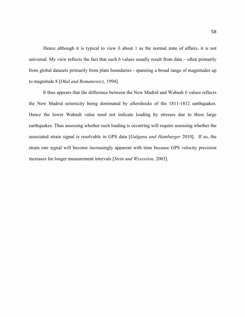
5.4 Apparent Mmax results for the eastern United States and eastern Canada ........... 70
5.5 Example of combined Mmax and b value results for MLE and LSQ ................... 71
5.6 b-value results for the eastern United States ....................................................... 72
5.7 b-value results for the eastern Canada ................................................................ 72
5.8 Combined Mmax and b value results .................................................................... 73
5.9 Recurrence time distribution for M7.6 earthquake ............................................. 73
5.10 Lower Rhine Embayment seismicity map .......................................................... 75
5.11 Apparent Mmax results for the Lower Rhine Embayment .................................... 76
5.12 b-value results for the Lower Rhine Embayment ................................................ 76
5.13 Percentage of simulation with differing standard deviations that recover
the simulations Mmax ........................................................................................... 78
6.1 Regional tectonic map of Arabia ........................................................................ 82
6.2 Cross-sections of the tomographic model ........................................................... 84

13
6.3 Shear wave velocity map at 150 km depth ......................................................... 86
6.4 Schematic tectonic model for the evolution of the Red Sea rift ......................... 88
7.1 Plot of horizontal over vertical spectral ratios for station A32A ........................ 94
7.2 Amplitude spectra and horizontal over vertical spectral ratios for all
stations ................................................................................................................ 99
7.3 Horizontal divided by vertical spectral ratios map of Minnesota ..................... 107
7.4 Spectral ratios versus soft sediment thickness .................................................. 108
7.5 Calculated and actual soft sediment thickness maps for Minnesota ................. 109
7.6 Error analysis plots for soft sediment thickness data ........................................ 110

14
CHAPTER 1
Introduction and Overview

15
1.1 Introduction
Rifts shape the Earth no matter what stage they are in, whether they are successfully
forming present-day oceans, failed and lying dormant within continents, or actively changing the
current landscape. My thesis has been a trek through many different topics with an underlying
theme of rifts. This trek was not intentional, but rather speaks to how pervasive the rifting
process is in our geologic endeavors.
Rifts are not only a scientific curiosity they play a major role in society by their
fundamental roles in sedimentary deposition and intraplate seismicity. Rifting events formed our
present day passive margins and influence the location of basins, both of which are where oil and
gas deposits are commonly found. Intraplate seismicity often occurs on old failed rifts because
they act as pre-existing zones of weakness. This seismicity is important to society because the
locations of intraplate earthquakes are currently unpredictable, in contrast to plate boundaries
where we expect earthquakes. Because the location of intraplate earthquakes is unknown, it is
unclear how much money should be allocated towards earthquake ‘proofing’ buildings in
intraplate regions.
This dissertation presents studies on the tectonics of a failed and active rift system and
studies of intraplate seismicity of failed and successful rift systems, as summarized next. Chapter
2 has been published in Geophysical Research Letters as Merino et al. [2013]. Chapter 3 has
been accepted in Geophysical Research Letters as Stein et al. [2014]. Chapter 4 has been
published in Seismological Research Letters as Merino et al. [2010]. Chapter 5 has been

16
submitted to Tectonophysics as Merino et al. [2014]. Chapter 6 has been published in
Geophysical Research Letters as Chang et al. [2011].
1.2 Chapter 2: Variations in Mid-Continent Rift magma volumes consistent with
microplate evolution
Modeling of gravity data along the central U.S.’s ~1.1 Ga failed Mid-Continent Rift
(MCR) shows systematic patterns in magma volume between and along the rift's two arms. The
volume of magma increases towards the Lake Superior region, consistent with magma flowing
away from a hotspot source there. The west arm experienced significantly more magmatism.
These patterns are consistent with a model in which the two rift arms acted as boundaries of a
microplate. The volume of magma along the west arm increases with distance from the Euler
pole, indicating that it acted essentially as a spreading ridge, whereas the much smaller magma
volumes along the east arm are consistent with its acting as a leaky transform. This view of the
rift system's evolution is compatible with the rift being part of an evolving plate boundary system
rather than an isolated episode of midplate volcanism.
1.3 Chapter 3: Was the Mid-Continent Rift part of a successful seafloor-spreading
episode?
This research was prompted in part by the results found in Chapter 2, where I showed
that the MCR could be viewed as part of a larger plate boundary system. Based on a result
indicating that the MCR was probably not formed by an isolated episode of midplate volcanism,

17
in Chapter 3, I suggest a plausible plate-tectonic scenario. I propose that the MCR formed as part
of the separation of Amazonia (Precambrian northeast South America) from Laurentia
(Precambrian North America) and became inactive once seafloor spreading was established. A
cusp in Laurentia’s apparent polar wander path recorded, at ~1.1Ga, by the MCR's volcanic
rocks likely reflects the rifting. This scenario is suggested by analogy with younger rifts
elsewhere and consistent with the geometry and timing of Precambrian rifting events including
the MCR's extension to southwest Alabama along the East Continent Gravity High, southern
Appalachian rocks having Amazonian affinities, and recent interpretation of large igneous
provinces in Amazonia.
1.4 Chapter 4: Comparison of Seismicity Rates in the New Madrid and Wabash Valley
Seismic Zones
Failed rift systems have societal importance because intraplate earthquakes often occur
on them. In 1811-1812, three large, ~M7, earthquakes occurred in the New Madrid Seismic Zone
(NMSZ), which is located on the failed Reelfoot rift. Based on historical accounts, the
magnitudes of these earthquakes were first inferreed to have been ~M8, and have been steadily
revised downward to ~M7. Li et al. [2005,2007] suggests that these large earthquakes should
have transferred stress to the Wabash Valley seismic zone, a geologically similar nearby region. I
explore this possibility by comparing seismic catalogs for New Madrid and the Wabash Valley. I
combined historical catalogs, starting after the 1811-1812 sequence, with recent instrumental

18
catalogs, to look at the Gutenberg-Richter frequency-magnitude relationship. A low slope,
denoted as the b value in the Gutenberg-Richter relationship, has been interpreted as being
indicative of a high stress region. I find that the Wabash Valley has a b value similar to the
background seismicity in the central U.S. In contrast, New Madrid has an anomalously high b
value that I attribute to a long aftershock sequence from the 1811-1812 events increasing the
number of small events and therefore the b value. This study prompted Chapter 5, which
explores the range in b values, and more importantly the maximum magnitude earthquake, that
we should expect to observe in such low seismicity intraplate regions given that we have a short
catalog.
1.5 Chapter 5: Have We Seen the Largest Earthquakes in Eastern North America?
The assumed magnitude of the largest future earthquakes, Mmax, is crucial in assessing
seismic hazard, especially for critical facilities like nuclear power plants. Absent any theoretical
basis, estimates of Mmax are made using various methods and often prove far too low, as for the
2011 Tohoku, Japan, earthquake. Estimating Mmax is particularly challenging within tectonic
plates, where large earthquakes are infrequent compared to the length of the available earthquake
history, vary in space and time, and sometimes occur on previously unrecognized faults. For
example, it is unclear whether the largest earthquakes possible along the eastern U.S seaboard
and eastern Canada have occurred. I explore this issue by generating synthetic earthquake
histories and sampling them over a few hundred years. The maximum magnitudes appearing
most often in the simulations are essentially those observed, and smaller than the simulation
19
maxima. Future earthquakes along both coasts may thus be significantly larger than those
observed to date.
1.6 Chapter 6: Mantle flow beneath Arabia offset from the opening Red Sea
Continental rifting involves a poorly understood sequence of lithospheric stretching,
volcanism, and mantle flow that evolves to seafloor spreading. I present new insight into the
tectonics of seafloor spreading in the Red Sea and Gulf of Aden associated with the three-arm
rift geometry as Africa splits into Nubia, Somalia, and Arabia. My tectonic analysis builds on
inversion of seismic traveltimes and waveforms beneath Arabia and surroundings performed by
Sung-Joon Chang and coworkers. Their results show low velocities beneath the southern Red
Sea and Gulf of Aden, consistent with active spreading. However, hot material extends not
below the northern Red Sea, but rather is offset eastward beneath Arabia, showing mantle flow
from the Afar hotspot. I start from the observation that this channel is located beneath volcanic
rocks that have erupted since rifting began 30 million years ago, indicating that the mantle flow
moves with Arabia. I propose that the absence of seafloor spreading in the northern Red Sea
reflects the offset flow. I model the kinematics of the three-plate system and show how this
geometry may evolve to spreading in the Northern Red Sea, rifting of Arabia, or both. This
situation has aspects of both active and passive rifting, showing that both can occur before
coalescing to seafloor spreading.

20
1.7 Chapter 7: Mapping sediment thickness in Minnesota with horizontal-to-vertical
spectral ratios from USArray data
Chapter 7 does not fall directly in the rifting theme, but presents an interesting technique
commonly used with very local seismic arrays, which I tested on a large array spanning part of
the Mid-Continent Rift. The spectral ratio between seismic noise recorded on the horizontal and
vertical components (HVSR) of USArray sites in Minnesota shows consistent spatial variations
in peak frequencies due to the variation in sediment thickness. The HVSR thus provides
reasonable estimates of the sediment thickness at sites. This result is consistent with earlier
studies that find this to be true when sediments are similar across a study region and their
impedance contrast with the basement rocks is strong.

21
CHAPTER 2
Variations in Mid-Continent Rift magma volumes consistent with microplate evolution

22
2.1. Introduction
The Mid-Continent Rift (MCR) is one of the most prominent features on the Bouguer
gravity map of the central United States (Figure 2.1). The rift formed at ~1.1Ga, recorded by two
pulses of magmatic activity lasting ~15Myr [White, 1997], making it one of the most extensive
paleorifts in the world [Hinze et al., 1997]. Petrologic and geochemical models favor the MCR
having been formed in the continental interior by a mantle plume [Davis and Green, 1997;
Nicholson et al., 1997; Vervoort et al., 2007]. Alternatively, many tectonic models view the rift
as having formed as a part of the Grenville orogeny [McWilliams and Dunlop, 1978; Gordon and
Hempton, 1986], which is the series of 1.3-0.9 Ga tectonic events associated with the assembly
of Rodinia [Whitmeyer and Karlstrom, 2007]. In such interpretations, northwest-directed
convergence at the southern margin of Laurentia (Proterozoic North America) caused extension
and magmatism to the northwest, including formation of the MCR. Volcanic activity was
followed by deposition of clastic sediments in subsiding basins and subsequent faulting of these
lithified sediments [Halls, 1982; Wold and Hinze, 1982]. Eventually, changing far-field stresses,
as the Grenville orogeny progressed, are proposed to have caused compression that slowed and
stopped the extension, leaving a failed rift [Cannon, 1994].
The 2000-km-long MCR, comparable in length to the presently active East African and
Baikal rifts, has two major arms meeting in the Lake Superior region. One extends
southwestward at least as far as Kansas, and the other extends southeastward at least through
Michigan. Because the rift is hidden beneath Phanerozoic sedimentary rocks, except where
exposed in the Lake Superior region, its location and geological characteristics are primarily

23
inferred from the gravity and magnetic anomalies, extrapolations from the outcrop area, seismic
reflection profiles, and a few basement drill holes.
Figure 2.1: Bouguer anomaly gravity map, from PACES database, of the central United States. White lines represent gravity profile and model locations, which are numbered and cross the anomalies that delineate the rift system. Lines 1, 2, 5, 8, and 9 are located near seismic lines.
Early active source seismic refraction studies indicate that the crust beneath Lake
Superior and portions of the west rift arm is thickened and anomalously dense [Ocola and
Meyer, 1973]. Similar crustal thickening was found in the east arm by Halls [1982]. Seismic
24
reflection data from the GLIMPCE program of active source studies across Lake Superior
[Cannon et al., 1989; Shay and Trehu, 1993] show that the crust was initially thinned to about
one-fourth of its original thickness. The resulting basin was filled with extrusive volcanics and
sediments, and volcanic underplating, producing a rift pillow, subsequently thickened the lower
crust. Such crustal rethickening has been identified in other rifts [Thybo and Nielsen, 2009].
Soon after magma had stopped erupting the normal faults were inverted to reverse motion,
presumably due to the Grenville orogeny [Cannon, 1994].
The highly magnetic and dense mafic igneous rocks filling the rift basin were juxtaposed
by high-angle reverse faulting against the less magnetic and less dense clastic rocks deposited in
the basins that originally overlaid them [King and Zietz, 1971]. The resulting gravity and
magnetic anomalies have been used to map the west arm of the rift, which extends into southern
Kansas and perhaps to southern Oklahoma [Adams and Keller, 1996]. Gravity and magnetic
anomalies also show that the rift continues into the basement beneath the Michigan basin [Oray
et al., 1973]. This interpretation has been confirmed by drilling in the Michigan basin that
encountered a thick section of clastic sedimentary rocks underlain by mafic volcanic rocks [Sleep
and Sloss, 1978], and reflection seismic studies [Brown et al., 1982] that detected the graben
structure sampled by the deep drill hole. The southern limit of the east arm is generally placed in
southeast Michigan, but a series of N-S trending gravity maxima that extend into Ohio, Kentucky
and Tennessee may be continuations of this arm [Halls, 1978; Keller et al., 1982]. Lidiak and
Zietz [1976] also suggested the presence of related rifts in the eastern Kentucky area.

25
2.2 Gravity Analysis
I examine variations in the volume of magmatic rocks along the east and west arms to
seek additional insight into the rift system's evolution. Numerous 2-D gravity and magnetic
models along parts of the MCR have been developed [Hinze et al., 1982; Wold and Hinze, 1982;
Van Schmus and Hinze, 1985; Cannon et al., 1989; Woelk and Hinze, 1991; Hinze et al., 1992;
Thomas and Teskey, 1994]. However, these models were constructed using a variety of software
and modeling schemes, making it difficult to compare results from different profiles. Hence I
conducted consistent modeling across both arms of the rift, allowing direct comparisons.
The gravity data (Figure 2.1) were compiled from the PACES database for land areas
[Keller et al., 2002, 2006; Hinze et al., 2005] and TOPEX satellite data for the Great Lakes
[Sandwell and Smith, 2009]. Only the Bouguer anomaly land data were used to create gravity
models.
Gravity profile locations were selected to give good spatial coverage of the rift arms, and
when possible, correlate with previous seismic reflection and gravity profiles. However, the
seismic data have poor resolution in the lower crust and hence do not significantly impact my
gravity models. Although, the Lake Superior region of the MCR has a significant amount of
seismic data, it was not modeled because the gravity data do not show a simple trend along the
rift. This choice also avoided the need to merge the higher quality land data with TOPEX
satellite data.
I used a generalized model inspired by a COCORP seismic reflection line in Kansas
[Serpa et al., 1984], as reinterpreted by Woelk and Hinze [1991]. This model has mafic

26
intrusions, a sedimentary basin overlying a large basaltic body, and large flanking sedimentary
basins. Thomas and Teskey [1994] infer that sedimentary rock densities in the northern MCR
range from 2.25 to 2.66 g/cm3 depending on the geologic unit. I use densities of 2.63g/cm3 in the
central basin, and 2.55 g/cm3 in the flanking basins.
For simplicity I treat the mafic intrusions as single magmatic bodies represented by
equilateral trapezoids with a density of 3.00 g/cm3 underlain by a Moho extracted from
CRUST2.0 [Bassin et al., 2000] (Figures 2.2, 2.3). A best fitting model for each profile was
found by a grid search (Figure 2.4). I also ran these models with mafic densities of 2.94 and 3.06
g/cm3. Two additional modeling schemes were also tested, one using Moho depths from NA07
[Bedle and van der Lee, 2009] (Figure 2.5, 2.6) and the second including a shallow basalt slab
beneath the central basin (Figure 2.7, 2.8). The volumetric trends are similar for all model sets.
2.3 Results and Interpretation
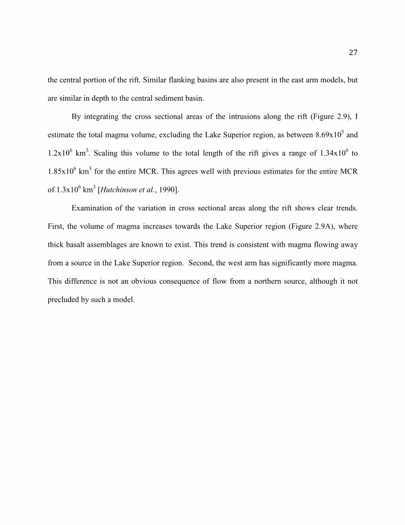
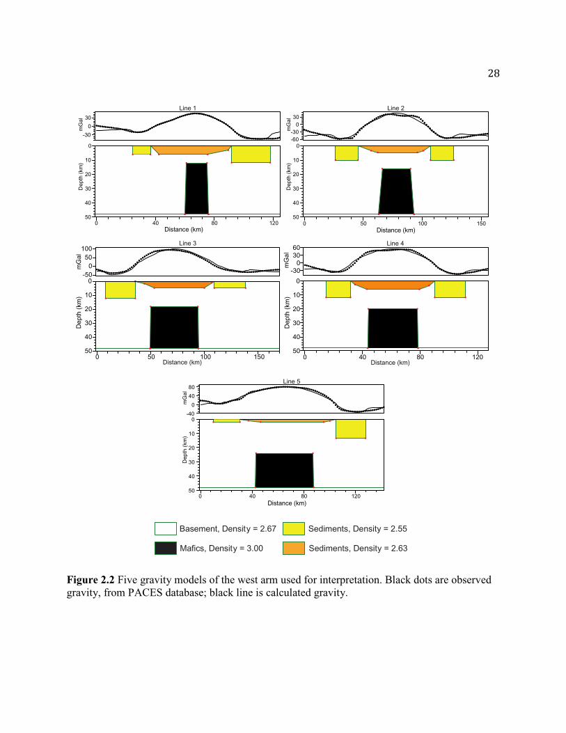
The models give insight into differences between the arms of the MCR. The Michigan
basin overlies the east arm, and the west arm has a higher central gravity anomaly with large
flanking negative anomalies. Figure 2.2 and 2.3 show how these differences manifest in the
gravity models. Because the Michigan basin is not centered on the rift, its sediments appear as a
gently dipping layer over the entire area that has little effect on the gravity models. The west
arm's more intense central anomalies are modeled by larger rift magmatic intrusions. The
negative anomalies on this arm's flanks are modeled as large sediment-filled flanking basins,
which are deeper than the central basin. This geometry reflects the tectonic inversion that raised
27
the central portion of the rift. Similar flanking basins are also present in the east arm models, but
are similar in depth to the central sediment basin.
By integrating the cross sectional areas of the intrusions along the rift (Figure 2.9), I
estimate the total magma volume, excluding the Lake Superior region, as between 8.69x10⁵ and
1.2x10⁶ km3. Scaling this volume to the total length of the rift gives a range of 1.34x10⁶ to
1.85x10⁶ km3 for the entire MCR. This agrees well with previous estimates for the entire MCR
of 1.3x10⁶ km3 [Hutchinson et al., 1990].
Examination of the variation in cross sectional areas along the rift shows clear trends.
First, the volume of magma increases towards the Lake Superior region (Figure 2.9A), where
thick basalt assemblages are known to exist. This trend is consistent with magma flowing away
from a source in the Lake Superior region. Second, the west arm has significantly more magma.
This difference is not an obvious consequence of flow from a northern source, although it not
precluded by such a model.
28
Figure 2.2 Five gravity models of the west arm used for interpretation. Black dots are observed gravity, from PACES database; black line is calculated gravity.
Basement, Density = 2.67
Mafics, Density = 3.00
Sediments, Density = 2.55
Sediments, Density = 2.63
-30
0
30
50
40
30
20
10
0
0 40 80 120
Line 1
mG
al
Distance (km)
Dep
th (
km)
-60-30
030
50
40
30
20
10
0
0 50 100 150
Line 2
mG
al
Distance (km)
Dep
th (
km)
mG
al
-500
50100
Dep
th (
km)
50
40
30
20
10
0
0 50 100 150
Line 3
Distance (km)
mG
al
-300
3060
Dep
th (
km)
50
40
30
20
10
0
0 40 80 120
Line 4
Distance (km)
-40
0
40
80
50
40
30
20
10
0
0 40 80 120
Line 5
mG
al
Distance (km)
Dep
th (
km)
29
Figure 2.3: Four gravity models of the east arm used for interpretation. Black dots are observed gravity, from PACES database; black line is calculated gravity.
mG
al
-100
102030
Dep
th (
km)
50
40
30
20
10
0
0 30 60 90
Line 6
Distance (km)
0
20
40
50
40
30
20
10
0
0 40 80 120
Line 7
mG
al
Distance (km)
Dep
th (
km)
mG
al
-20
0
20
Dep
th (
km)
50
40
30
20
10
0
0 50 100 150
Line 8
Distance (km)
-20
0
20
40
50
40
30
20
10
0
0 50 100 150
Line 9
mG
al
Distance (km)
Dep
th (
km)
Basement, Density = 2.67
Mafics, Density = 3.00
Sediments, Density = 2.55
Sediments, Density = 2.63
Michigan basin sediments Density = 2.63

30
Figure 2.4: Example of misfit plots for mafic trapezoid size. The X/Y axes refer to the size of base 1, and 2 of the basaltic trapezoid in the gravity models. Each contour plot is for a trapezoid of a different height. The grey area of each plot is excluded because base 1 is not allowed to be larger than base 2. Black dot shows the model that was chosen.

31
Figure 2.5: Gravity models of the west arm using the Moho depth from NA07. Black dots are observed gravity, from PACES database; black line is calculated gravity.
mG
al
-30
0
30
0 40 120Distance (km)
Dep
th (
km)
40
30
20
10
0
80
Line 1
mG
al
-60-30
030
0 50 100 150Distance (km)
Dep
th (
km)
50
40
30
20
10
0
Line 2
mG
al
0 50 100 150Distance (km)
Dep
th (
km)
50
40
30
20
10
0
Line 3
-50
0
50
100
mG
al
0 40 80 120Distance (km)
Dep
th (
km)
50
40
30
20
10
0
Line 4
-300
3060
mG
al
0 40 80 120Distance (km)
Dep
th (
km)
50
40
30
20
10
0
Line 5
-40
0
40
80
West Arm
Basement, Density = 2.67
Mafics, Density = 3.00
Sediments, Density = 2.55
Sediments, Density = 2.63

32
Figure 2.6: Gravity models of the east arm using the Moho from NA07. Black dots are observed gravity, from PACES database; black line is calculated gravity.
mG
al
-20
0
20
40
0 50 100 150Distance (km)
Dep
th (
km)
50
40
30
20
10
0
Line 9
-20-10
01020
mG
al
0 50 100 150Distance (km)
Dep
th (
km)
40
30
20
10
0
Line 8
-100
10203040
mG
al
0 40 80 120Distance (km)
Dep
th (
km)
40
30
20
10
Line 7
0
mG
al
0 30 60 90Distance (km)
Dep
th (
km)
40
30
20
10
0
Line 6
-100
102030
East Arm
Basement, Density = 2.67
Mafics, Density = 3.00
Sediments, Density = 2.55
Sediments, Density = 2.63
Michigan basin sediments Density = 2.63

33
Figure 2.7: Gravity models of the west arm including a shallow basalt slab 3km thick with a width the same as the central sediment basin. Black dots are observed gravity, from PACES database; black line is calculated gravity.
mG
al
-30
0
30
0 40 120Distance (km)
Dep
th (
km)
40
30
20
10
0
80
Line 1
mG
al
-60-30
030
0 50 100 150Distance (km)
Dep
th (
km)
50
40
30
20
10
0
Line 2
mG
al
-60
0
60
120
0 50 100 150Distance (km)
Dep
th (
km)
50
40
30
20
10
0
Line 3
mG
al
-400
40
0 40 80 120Distance (km)
Dep
th (
km)
50
40
30
20
10
0
Line 4
mG
al
-50
0
50
100
0 40 80 120Distance (km)
Dep
th (
km)
50
40
30
20
10
0
Line 5
West Arm
Basement, Density = 2.67
Mafics, Density = 3.00
Sediments, Density = 2.55
Sediments, Density = 2.63

34
Figure 2.8: Gravity models of the east arm including a shallow basalt slab 3km thick with a width the same as the central sediment basin. Black dots are observed gravity, from PACES database; black line is calculated gravity.
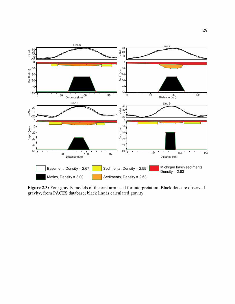
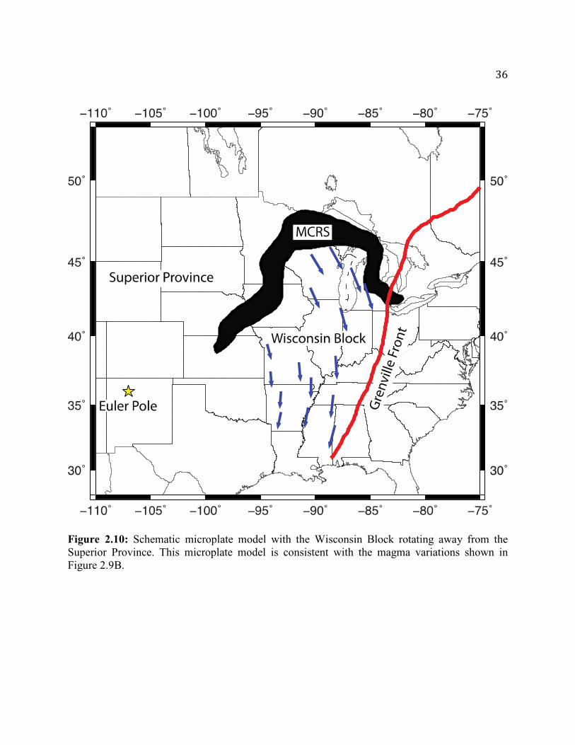
However, the magma volumes are consistent with a model (Figure 2.10) in which the two
rift arms acted as boundaries of a microplate. Chase and Gilmer [1973] found an Euler pole for
such a model by treating offsets in the gravity maxima as transform faults, and using the width of
the central gravity anomaly as a measure of total spreading. As shown, the volume of magma I
infer along the west arm increases with distance from the Euler pole (Figure 2.9B). Thus the
mG
al
-200
2040
0 30 60 90Distance (km)
Dep
th (
km)
40
30
20
10
0
Line 6
mG
al
-200
204060
0 40 80 120Distance (km)
Dep
th (
km)
40
30
20
10
0
Line 7
mG
al
-30
0
30
0 50 100 150Distance (km)
Dep
th (
km)
40
30
20
10
0
Line 8
mG
al-20
0
20
40
0 50 100 150Distance (km)
Dep
th (
km)
50
40
30
20
10
0
Line 9
East Arm
Basement, Density = 2.67
Mafics, Density = 3.00
Sediments, Density = 2.55
Sediments, Density = 2.63
Michigan basin sediments Density = 2.63

35
results of analyzing more recent gravity data are also consistent with the microplate model.
Moreover, the much smaller volumes of magma along the east arm are consistent with this arm
being a leaky transform, along which trans-tensional motion permits some magmatism.
Figure 2.9: A) Cross sectional magma areas in the models plotted as a function of distance from the Lake Superior region. The areas increase toward the Lake Superior region and the west arm has significantly more magma than the east arm. B) Cross sectional magma areas in the models plotted against distance from the Chase and Gilmer [1973] Euler pole. Black bars show the range in cross sectional areas for the other four modeling schemes.
Viewing the MCR's evolution as showing rotation of a rigid microplate does not preclude
its having been started by a mantle plume. However, this view is consistent with the rift having
been part of an evolving regional plate boundary system [Whitmeyer and Karlstrom, 2007] rather
than an isolated episode of midplate volcanism.
0
200
400
600
800
1000
1200
1400
1600
0 500 1000 1500 2000 2500
Cro
ss S
ectio
nal A
rea
(km
2 )
Distance From Euler Pole (km)
Mid-Continent Rift Magma Variation
0
200
400
600
800
1000
1200
1400
1600
0 200 400 600 800 1000 1200
Cro
ss S
ectio
nal A
rea
(km
2 )
Distance From Presumed Lake Superior Hotspot (km)
Mid-Continent Rift Magma Variation
A B West armEast arm
West armEast arm
1
2
3
45
67
89 1
2
3
45
67
89
36
Figure 2.10: Schematic microplate model with the Wisconsin Block rotating away from the Superior Province. This microplate model is consistent with the magma variations shown in Figure 2.9B.

37
CHAPTER 3
Was the Mid-Continent Rift part of a successful seafloor-spreading episode?

38
3.1 Introduction
One of the most prominent features on gravity and magnetic maps of North America is
the Mid-Continent Rift (MCR), a band of buried mafic igneous rocks extending from Lake
Superior (Figure 3.1). These rocks outcrop from Minnesota through Wisconsin and the Upper
Peninsula of Michigan. To the south the rift is deeply buried by younger sediments, but easily
traced because the igneous rocks are dense and highly magnetized [Hinze et al., 1992; King and
Zietz, 1971]. Its west arm extends at least to Oklahoma, and perhaps Texas and New Mexico via
similar-age diffuse volcanism [Adams and Keller, 1996]. The east arm goes through Michigan
and extends southward along the Fort Wayne Rift (FWR) and East Continent Gravity High
(ECGH) to Alabama [Keller et al., 1982]. In Alabama, the gravity and magnetic anomalies have
been interpreted as indicating mafic rocks [Steltenpohl et al., 2013].
3.2 Gravity Analysis
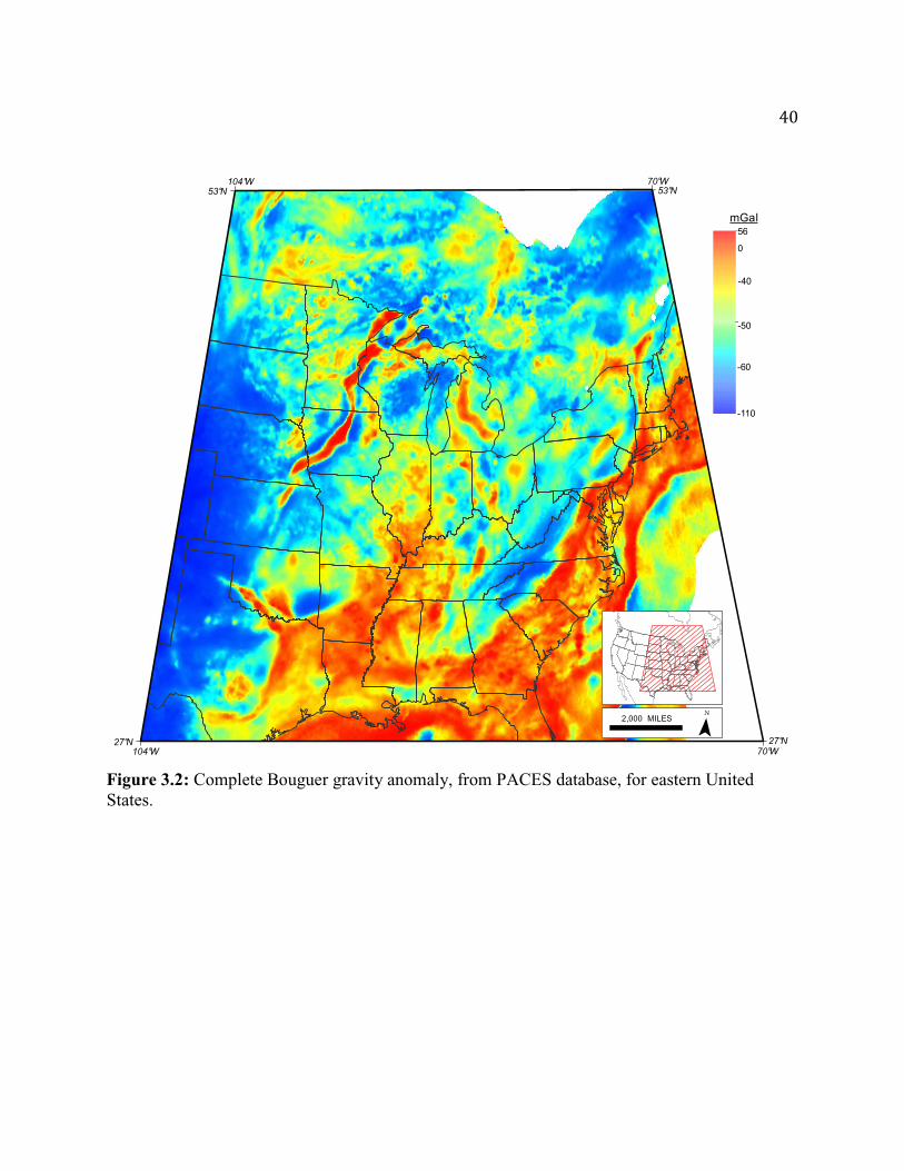
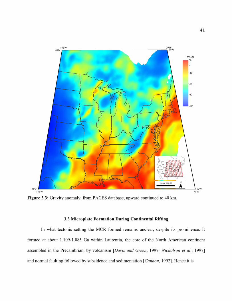
The residual Bouguer anomaly gravity map (Figure 3.1) was calculated by upward
continuing complete Bouguer anomaly (CBA) data (Figure 3.2) to 40 km (Figure 3.3) and
subtracting the result point-by-point from the CBA grid. Upward continuation acts as a low pass
filter that attenuates shorter wavelength anomalies and so smoothes the data [Blakely, 1996], as
demonstrated in Figure 3.3. The gravity highs associated with the MCR, FWR, and ECGH still
appear strongly, trending in the same directions as in the CBA map. Subtracting the upward
continuation result removes the long wavelength anomalies and hence emphasizes shallower
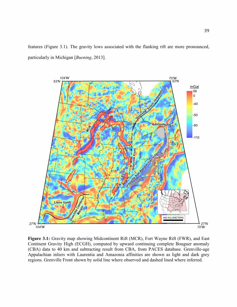
39
features (Figure 3.1). The gravity lows associated with the flanking rift are more pronounced,
particularly in Michigan [Buening, 2013].
Figure 3.1: Gravity map showing Midcontinent Rift (MCR), Fort Wayne Rift (FWR), and East Continent Gravity High (ECGH), computed by upward continuing complete Bouguer anomaly (CBA) data to 40 km and subtracting result from CBA, from PACES database. Grenville-age Appalachian inliers with Laurentia and Amazonia affinities are shown as light and dark grey regions. Grenville Front shown by solid line where observed and dashed lined where inferred.
MC
R
Llano Uplift
Grenville
AdirondacksGre
nville
Age
Appal
achia
n Inlie
rs
Front
(map
ped)
FWR
EC
GH G
r en
vil le
Fr o
nt
Oua
chita
Cam
bria
n
Mar
gin
104°W53°N
70°W53°N
70°W27°N
104°W27°N
400 KILOMETERS
-110
-40
-60
-50
056
mGal
40
Figure 3.2: Complete Bouguer gravity anomaly, from PACES database, for eastern United States.
104°W53°N
70°W53°N
70°W27°N
104°W27°N
MILES2,000
-110
-40
-60
-50
0
56mGal
41
Figure 3.3: Gravity anomaly, from PACES database, upward continued to 40 km.
3.3 Microplate Formation During Continental Rifting
In what tectonic setting the MCR formed remains unclear, despite its prominence. It
formed at about 1.109-1.085 Ga within Laurentia, the core of the North American continent
assembled in the Precambrian, by volcanism [Davis and Green, 1997; Nicholson et al., 1997]
and normal faulting followed by subsidence and sedimentation [Cannon, 1992]. Hence it is
104°W53°N
70°W53°N
70°W27°N
104°W27°N
MILES2,000
-110
-40
-60
-50
0
56mGal

42
commonly viewed as a type example of a failed rift that formed and died within a continental
interior, far from its margins, not associated with a plate boundary or successful rifting/seafloor-
spreading event.
A difficulty with this view is that many intracontinental rifts are associated with plate
boundary reorganizations (Figure 3.4). Present-day continental extension in the East African Rift
(EAR) and seafloor spreading in the Red Sea and Gulf of Aden form a classic three-arm rift
geometry as Africa splits into Nubia, Somalia, and Arabia. GPS and earthquake data show that
the opening involves several microplates between the large Nubian and Somalian plates [Saria et
al., 2013]. If the EAR does not evolve to seafloor spreading and dies, in a billion years it would
appear as an isolated intracontinental failed rift similar to the MCR.
Another analogy is the West Central African Rift (WCAR) system formed as part of the
Mesozoic opening of the South Atlantic. Reconstructing the fit between Africa and South
America without overlaps and gaps and matching magnetic anomalies requires microplate
motion with up to 95 km extension within continents [Moulin et al., 2010; Seton et al., 2012].
These rifts failed about when seafloor spreading started along the whole boundary between
South America and Africa, illustrating that intracontinental extension can start as part of
continental breakup and end when full seafloor spreading is established.
Although similar rift systems occur earlier in the geological record, it is harder to identify
them and establish their history because the plates involved are now widely separated and
sometimes affected by subsequent continent-continent collisions that overrode the rifted

43
continental margins. Also, the oceanic seafloor with its magnetic reversal record that formed
after the continents rifted has been subducted.
As just discussed, active rifts within continents with similar lengths to the MCR form
boundaries of microplates within the evolving boundary zone between major plates. Similarly,
the MCR can be described as part of a microplate’s boundary [Chase and Gilmer, 1973]. Magma
volumes inferred from gravity modeling (Chapter 2) [Merino et al., 2013] are consistent with the
western arm opening mainly by extension and the eastern arm in Michigan as a leaky transform.
Figure 3.4: Microplate formation during continental rifting. (A) Present rifting of Africa into three major plates and three microplates, after Saria et al. [2013]. (B) Four-microplate geometry of the west central African rift system, formed during the Mesozoic opening of the South Atlantic, after Moulin et al. [2010].

44
3.4 Apparent Polar Wander Path
The apparent polar wander path for Laurentia in Figure 3.5 contains paleomagnetic poles
from Elming et al. [2009] and Swanson-Hysell et al. [2009]. Prior to the formation of the MCR I
use the 1.235 Ga pole for the Sudbury Dykes (1, blue), 1.204 Ga Upper Bylot (2, blue), and
1.141 Ga pole for the Abitibi Dykes (3, blue). For the MCR, I primarily use the best-dated sites,
those from Mamainse Point (4-8, red) determined by Swanson-Hysell et al. [2009]. These dates
[http://www.swanson-hysell.org/research/keweenawan/] range from about 1.109-1.094 Ga with
the exception of one somewhat younger paleopole. I also use two somewhat younger paleopoles
from Swanson-Hysell et al. [2009] for the ~1.095 Ga Portage Lake Lavas (9, red) and the ~1.087
Ga Lake Shore Traps (10, red).
For the post-rift sediments of the MCR [Ojakangas et al., 2001] I use only those from the
Oronto Group (Copper Harbor Conglomerate (oldest, 11, green), Nonesuch Shale (12, green) and
Freda Sandstone (youngest, 13, green). The Copper Harbor Conglomerate pole plots near the
igneous MCR path, unlike the two younger formations. Halls and Palmer [1981] note that the
direction of magnetization of the Copper Harbor sediments is "virtually indistinguishable" from
the Portage Lake volcanics and thus may have been reset due to the interlayering volcanic
intrusions and/or are of similar age. Thus these sediments may have been deposited during the
rifts opening. Because the Bayfield Group near the MCR may be significantly younger than the
Oronto Group, I do not use its paleomagnetic pole. The youngest pole shown is for the 1.015 Ga
Halliburton Intrusions (14, black).

45
3.5 Laurentia, Amazonia, and the MCR
I propose that the MCR’s formation and shutdown was part of the evolution of the plate
boundary between Laurentia and neighboring plates. The location and timing of key events
relevant to the MCR’s evolution fit nicely into the known history of plate interactions. Absent a
seafloor spreading record, reconstructions based on paleomagnetic data provide a general view
of this evolution.
Interpretation of a loop in Laurentia's apparent polar wander (APW) path (Figure 3.5A),
often referred to as the Logan Loop, has been unclear. The loop could have resulted from an
irregularity in the earth's magnetic field ~1.11 Ga (a reversal asymmetry or non-dipolar field
component) or an unspecified plate tectonic event [Halls and Pesonen, 1982]. Volcanic rocks in
the MCR formed during this period and hence record the change in the earth's magnetic field and
Laurentia's APW path. Using high-resolution paleomagnetic data, Swanson-Hysell et al. [2009]
showed that there was no asymmetry in the reversals. I thus propose that the cusp in Laurentia’s
APW path [Elming et al., 2009; Swanson-Hysell et al., 2009] likely reflects plate motion changes
due to rifting, in part involving the MCR. Cusps in APW paths have been observed when
continents separate and a new ocean forms between the two fragments. For example, cusps in
North America’s path coincide with the 90 Ma rifting of Europe from North America and the
180 Ma rifting of Gondwana from Laurasia [Gordon et al., 1984].
Likely the ~1.11 Ga cusp reflects rifting between Laurentia and Amazonia (Precambrian
northeast South America). In some models, Amazonia was in contact with Laurentia ~1.2 Ga
[Tohver et al., 2002] (Figure 3B), moved left-laterally until about 1.12 Ga [Tohver et al., 2006],

46
and then moved away. These interactions are recorded in the rock record. The absence of
igneous rocks younger than ~1.23 Ga in the Llano uplift (Texas) area is interpreted as indicating
the ending of a subduction episode [Mosher et al., 2008]. By 1.2 Ga, intracontinental rifting in
Amazonia is recorded in the Nova Brasilândia region [Teixeira et al., 2010]. Amazonia’s
subsequent left lateral motion relative to Laurentia is recorded by deformation in the Ji-Paraná
shear network from 1.18-1.12 Ga [Tohver et al., 2006]. The beginning of its separation from
Laurentia is indicated by recently dated ~1.110 Ga mafic rocks in Rincón del Tigre and
Huanchaca in the SW corner of the Amazon craton [Ernst et al., 2013] and renewed igneous
activity in Nova Brasilândia [Teixeira et al., 2010; Tohver et al., 2006].

47
Figure 3.5: (A) Apparent polar wander path for Laurentia, showing cusp approximately at onset of MCR volcanism (1.109 Ga) that likely reflects the rifting. Poles from Elming et al. [2009] and Swanson-Hysell et al, [2009]. (B) Reconstruction of plate positions before Laurentia-Amazonia separation, after [D'Agrella-Filho et al., 2008; Elming et al., 2009; Tohver et al., 2002], schematic rift geometry, and relevant features.

48
Because the MCR formed while Amazonia rifted from Laurentia, it seems likely that the
rifting events are related. Mafic dikes and other intrusions started north and west of Lake
Superior ~1.15 Ga and continued for 40 my [Heaman et al., 2007]. The huge volume of MCR
volcanism started around Lake Superior at ~1.109 Ga [Davis and Green, 1997], approximately
the same time as volcanism within the SW part of the Amazonian craton [Ernst et al., 2013].
3.6 Reconstructions Using Paleomagnetic Data
Paleomagnetic reconstructions (Figure 3.5B) [D'Agrella-Filho et al., 2008] place SW
Amazonia near the southern end of the East Continent Gravity High, an extension of the MCR’s
eastern arm. Hence the MCR probably connected to the extensional system that separated the
two continents. In this scenario, MCR volcanism ended once motion was taken up by seafloor
spreading between Laurentia and Amazonia.
After extension ended, normal faults in the MCR region were reactivated as reverse faults
~1.06±0.02 Ga [Cannon et al., 1993]. The compression is assumed to be associated with
collisional tectonics during the Grenville orogeny [Soofi and King, 2002], the ~1.3-0.98 Ga
assembly of Amazonia and other continents into the supercontinent of Rodinia [Dalziel et al.,
2000; Hoffman, 1991; McLelland et al., 2010]. Most of the best-exposed Grenville deformation
is found along the eastern Canadian margin. Grenville-age orogenic events are also found in the
south and southwestern United States and South America. The Grenville Front in Canada is the
boundary between the deformed Grenville fold and thrust belt and areas in the interior of
Laurentia largely unaffected by Grenville deformation. In most of the United States this

49
boundary is inferred from gravity and magnetic data. In Texas the boundary is called the Llano
Front and associated deformation is recorded in the rocks of the Llano uplift south of the front.
3.7 Discussion
The scenario proposed here is consistent with the recent recognition that the central and
south Appalachians were not part of Laurentia before the Grenville orogeny. Although
Grenville-age Appalachian inlier rocks in the Adirondacks have affinities to Grenville rocks in
Canada, most of those to the south are more similar to Amazonia [Fisher et al., 2010; Loewy et
al., 2003; McLelland et al., 2010]. They lack a petrologic signature of the ~1.5-1.3 Ga Granite-
Rhyolite province formed within Laurentia [Fisher et al., 2010], suggesting that they were not
part of Laurentia before the Grenville orogeny.
My scenario addresses events 1.1 billion years ago, when the geologic record is limited
and sparse because many areas are deeply buried, have been eroded, or have been subsequently
deformed. Because many aspects of Laurentia – Amazonia rifting and Rodina’s assembly during
the Grenville remain unresolved, my scenario is schematic. I attribute MCR formation to
Laurentia – Amazonia rifting, which – depending on unresolved issues in reconstruction - also
may be related to contemporaneous large igneous provinces and possible rifting in the Indian,
Congo, and Kalahari cratons [Ernst et al., 2013] recorded by APW path cusps [Gose et al.,
2013].
In my model rifting does not result from Grenville collisional events, as sometimes
proposed [Gordon and Hempton, 1986]. Instead, it results from rifting during the Grenville at a

50
time when compression was absent or occurred elsewhere. Probably because of lack of
exposure, it is commonly assumed that Grenville-age tectonics along the present U.S. to Mexico
margin should have been similar to those recorded by Grenville-age rocks exposed in Canada.
However, this need not have been the case. This margin’s length is comparable to that from
Turkey to Gibraltar, along which tectonics varies with space and time during the Cenozoic.
Similarly, events associated with the formation of the Paleozoic Appalachian-Caledonian
mountains differ along the length of the system.
In summary, rather than viewing the largest gravity and magnetic anomaly within the
North American craton as an exotic feature, I view the MCR’s formation and evolution in a plate
tectonic context consistent with what we know of plate motions then and analogous rifting
events. Additional data will be required to test this scenario. One promising source is the
EarthScope program, which is acquiring new data about lithospheric structure below the MCR
[Shen et al., 2013; Stein et al., 2011]. Data across its possible extensions to the south and the
Grenville Front will show more about these structures and possible relations between them. My
model suggests that the East Continent Gravity High should appear similar to the MCR, and that
there may be additional evidence of the rifted margin between Amazonia and Laurentia.

51
CHAPTER 4
Comparison of Seismicity Rates in the New Madrid and Wabash Valley Seismic Zones

52
4.1 Introduction
The Wabash Valley seismic zone in southern Illinois and Indiana is the northeastern
extension of the New Madrid seismic zone (Figure 4.1). Like New Madrid, the Wabash zone is
underlain by a failed Precambrian failed rift, which plays a role in controlling the recent faulting
[Braile et al., 1986; Sexton et al., 1986; Bear et al., 1997]. Paleoliquefaction deposits indicate the
past occurrence of large earthquakes in the Wabash zone [Obermeier, 1998] that may have been
comparable to those that occurred in the New Madrid zone in 1811-1812 [Hough et al., 2000].
The two areas seem likely to be mechanically coupled in that stress transfer following large
earthquakes in one could affect earthquake occurrence in the other [Mueller et al., 2004].
Numerical modeling indicates that stress transfer following the 1811-1812 New Madrid
earthquakes may be loading faults in the Wabash zone [Li et al., 2005; 2007].
Despite their similarities, the two zones have an intriguing difference in seismicity rates
[Stein and Newman, 2004]. This difference is shown in Figure 4.2A by comparison of frequency-
magnitude plots. The plots combine the CERI catalog of seismologically recorded small
earthquakes spanning January 1975 - June 2010
(http://www.ceri.memphis.edu/seismic/catalogs/cat_nm.html) and the Nuttli catalog of historic
earthquakes for 1804 - 1974 with magnitudes out to magnitude 6.2 [Nuttli, 1974].
4.2 Results
Both areas show a Gutenberg-Richter distribution of seismicity, log10N = a – bM, where
the logarithm of the annual number (N) of earthquakes above a given magnitude (M) decreases

53
linearly with magnitude (Figure 4.2A). A least squares fit to the New Madrid zone data (defined
as 35-38°N, 88-91°W) yields a=3.45 and b=0.95 � 0.02. The Wabash zone (treated here as
37.6°-39.7°N, 85.8°-88.75°W) yields a=2.13 and b=0.72 � 0.03. (These areas, defined as
rectangular for simplicity, have a slight overlap). Hence the New Madrid and Wabash zones have
similar numbers of magnitude 5-6 earthquakes, but the larger slope (b) indicates that New
Madrid has more small earthquakes.

54
Figure 4.1: Seismicity map of central United States. Main 1811-1812 earthquakes represented by stars. New Madrid Seismic Zone (NMSZ), Wabash Valley Seismic Zone (WVSZ), Reelfoot Rift (RFR).

55
Figure 4.2: (A) Frequency-magnitude plots for New Madrid and Wabash seismic zones and (B) comparison of these zones with the central U.S.
The b value difference does not appear to result from the limitations of the data, which
are common to both zones. This analysis combines instrumentally determined magnitudes for
recent smaller earthquakes with ones inferred from historical records of older larger earthquakes.
The linear trend continues relatively smoothly between the two data types. The results are robust
in that they are consistent with those of previous studies combining the historical data with
progressively longer instrumental records [Nuttli, 1974; Johnston and Nava, 1985; Stein and
Newman, 2004]. Catalog incompleteness appears not to be a problem given the lack of a falloff
at low magnitudes considered. Thus although the specific b values derived here (as in any area)
depend on the dataset and analysis method used, the difference in b values between the two
seismic zones seems real.
Historical
1 2 3 4 5 7Magnitude
6
0.01
0.1
1
10
100
Ear
thqu
ake
Rat
e 1/
yr
1 2 3 4 5 7Magnitude
6
0.01
0.1
1
10
100
Ear
thqu
ake
Rat
e 1/
yr
New MadridWabash
Central U.S
Central U.S without NewMadrid and Wabash
A B

56
4.3 Discussion
I see two possible causes for the b value difference. The first is that the Wabash area has
a low b value. A low b value could indicate high stressing rates on faults [Scholz, 1968; Wiemer
and Wyss, 1997]. Hence a low value in the Wabash could mean a higher stressing rate there than
in the New Madrid zone for the period spanned by these data, since 1812. This would be
consistent with the predicted stress migration following the large 1811-1812 earthquakes [Li et
al., 2005; 2007].
Alternatively, the New Madrid zone has a high b value. This situation could arise if many
of the earthquakes there are aftershocks of the large 1811-1812 earthquakes [Ebel et al., 2000;
Stein and Newman, 2004; Hough, 2009; Stein and Liu, 2009]. b values for many aftershock
sequences are higher than those found by including the main shocks [Frohlich and Davis, 1993].
This may be the case here, because the data used do not include the three main shocks, owing to
the complexities in assessing their magnitudes [Hough et al., 2000].
Given that b values for different areas vary widely, largely between 0.5 and 2.0 [Frohlich
and Davis, 1993], I assess whether the values for the two areas are “high” or “low” by
comparing them to those for the entire central U.S., defined here as 34.5°-41°N, 85°-92°W
(Figure 4.1). For this region, a=3.57 and b=0.9 � 0.02 (Figure 4.2B). However, considering
earthquakes in this region but excluding both the New Madrid and Wabash zones yields a=0.9
and b=0.83 � 0.02, because most small events are in the New Madrid zone.
Thus the Wabash valley b value is lower than New Madrid’s but closer to that for the central
U.S. excluding both zones. Hence I view the Wabash value as more typical of the central U.S.,
57
and New Madrid value as unusually high.
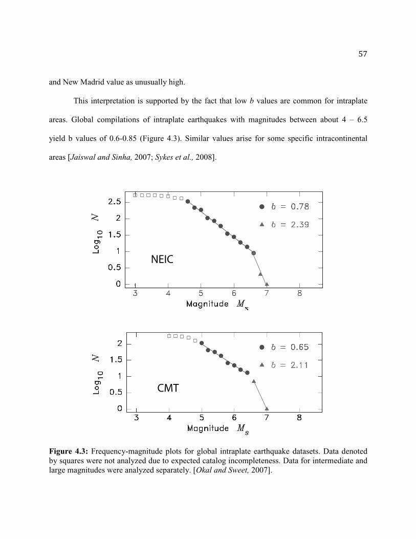
This interpretation is supported by the fact that low b values are common for intraplate
areas. Global compilations of intraplate earthquakes with magnitudes between about 4 – 6.5
yield b values of 0.6-0.85 (Figure 4.3). Similar values arise for some specific intracontinental
areas [Jaiswal and Sinha, 2007; Sykes et al., 2008].
Figure 4.3: Frequency-magnitude plots for global intraplate earthquake datasets. Data denoted by squares were not analyzed due to expected catalog incompleteness. Data for intermediate and large magnitudes were analyzed separately. [Okal and Sweet, 2007].
58
Hence although it is typical to view b about 1 as the normal state of affairs, it is not
universal. My view reflects the fact that such b values usually result from data – often primarily
from global datasets primarily from plate boundaries - spanning a broad range of magnitudes up
to magnitude 8 [Okal and Romanowicz, 1994].
It thus appears that the difference between the New Madrid and Wabash b values reflects
the New Madrid seismicity being dominated by aftershocks of the 1811-1812 earthquakes.
Hence the lower Wabash value need not indicate loading by stresses due to these large
earthquakes. Thus assessing whether such loading is occurring will require assessing whether the
associated strain signal is resolvable in GPS data [Galgana and Hamburger 2010]. If so, the
strain rate signal will become increasingly apparent with time because GPS velocity precision
increases for longer measurement intervals [Stein and Wysession, 2003].

59
CHAPTER 5
Have We Seen the Largest Earthquakes in Eastern North America?

60
5.1 Introduction
The 2011 Virginia earthquake that shook much of the northeastern U.S. showed that
earthquakes large enough to cause significant damage occur in eastern North America, a
‘stable’ intraplate region [Wolin et al., 2012] (Figure 5.1). Assessing the hazard of such
earthquakes poses major unresolved issues. Hazard maps, giving the maximum shaking
expected in an area with a certain probability in some time period [Cornell, 1968], require
assuming where and when large earthquakes will occur and how large they will they be.
However, the recent Tohoku, Haiti, and Wenchuan earthquakes illustrate that earthquakes
much larger than expected occur in many places [Geller, 2011; Gulkan, 2013; Kerr, 2011;
Peresan and Panza, 2012; Stein and Okal, 2011; Wyss et al., 2012]. Such surprises arise
because parameters required to reliably estimate the hazards are often poorly known
[Stein et al., 2012].
A crucial parameter is Mmax, the magnitude of the largest earthquake expected on a
fault or in an area [Stein et al., 2012]. The Tohoku, Haiti, and Wenchuan earthquakes were
more damaging than expected because they were much larger than the Mmax assumed in
hazard planning [Kanamori, 2011; Sagiya, 2011; Witze, 2009]. Unfortunately, no theoretical
basis exists to infer Mmax. Even where we know the long-term rate of motion across a plate
boundary fault, or the deformation rate across an intraplate zone, neither predict how
strain will be released. Strain release can occur seismically or aseismically, and seismic
strain release can occur via earthquakes with different magnitudes and rate distributions.
As a result, quite different Mmax estimates can be made [Kagan and Jackson, 2013;

61
Kijko, 2004; U.S Nuclear Regulatory Commission, 2012]. Because all one can say with
certainty is that Mmax is at least as large as the largest earthquake in the available record, it
was earlier practice to use that magnitude or add an increment. However, because catalogs
are often short relative to the average recurrence time of large earthquakes [Bell et al.,
2013; McGuire, 1977; Stein and Newman, 2004], larger earthquakes than anticipated often
occur. Another approach is to identify faults and use relations between fault length and
earthquake magnitude [Wells and Coppersmith, 1994] to infer Mmax. Other approaches
extrapolate from current catalogs [Kijko, 2004] or combine areas presumed to be
geologically similar to sample more large earthquakes [Kagan and Jackson, 2013; U.S.
Nuclear Regulatory Commission, 2012].
Estimating Mmax is challenging at plate boundaries, where known plate motion rates
can be compared to earthquake records on known faults to infer the slip in, and thus
magnitude of, large earthquakes. The situation is more complicated within plates, where
deformation rates are poorly known, large earthquakes are rarer and variable in space and
time, and often occur on previously unrecognized faults [Camelbeeck et al., 2007; Clark et
al., 2011; Crone et al., 2003; Leonard et al., 2014; Liu et al., 2011].
I explore this issue for eastern North America and Lower Rhine Embayment (LRE),
which includes portions of Belgium, Germany, and the Netherlands [Camelbeeck et al.,
2007]. Notable events along the U.S. margin include the 1755 Cape Ann Massachusetts and
1886 Charleston earthquakes. Larger earthquakes are known along the Canadian margin,
notably the 1929 Grand Banks and 1933 Baffin Bay events. Thus this passive continental

62
margin, like others, has a moderate level of seismicity [Schulte and Mooney, 2005; Stein et
al., 1979; Stein et al., 1989; Wolin et al., 2012]. The largest known event in the LRE is the M
5.7, 1756 Düren earthquake.
A challenge in assessing the earthquakes’ hazard is that we know little about their
causes, partly because they are relatively rare due to the slow deformation at such margins.
They may reflect reactivation of faults created by previous continental collision and
breakup, given that passive margins are often reactivated [Cloetingh et al., 2008].
Geodynamic modeling predicts stresses from variations in topography and crustal
structure across the margin, combined with sublithospheric mantle flow [Ghosh et al.,
2013].

63
Figure 5.1: Seismicity of the eastern North American continental margin taken from ANSS
and NEDB catalogs. Red and blue dots correspond to the U.S and Canadian margins
respectively. Major historical events are also shown.

64
A crucial issue is how much to rely on past large earthquakes, as illustrated by
successive Geological Survey of Canada hazard maps [Adams, 2011; Wolin et al., 2012]. The
1985 suite of maps concentrate hazard at the sites of the Grand Banks and Baffin Bay
earthquakes, assuming that these recently active areas are especially hazardous. The 2005
maps have an additional ribbon of hazard along the passive margin, assuming that similar
earthquakes can occur anywhere along the margin.
The observed seismicity may be an imperfect sample of a more uniform seismicity
as suggested by seismicity between the Grand Banks and Baffin Bay, some of which may be
aftershocks of prehistoric earthquakes [Basham and Adams 1983; Wolin et al., 2012].
Simulations with short catalogs yield apparent concentrations and gaps that are artifacts of
the sampling [Swafford and Stein, 2007]. Similarly, although seismicity in the eastern U.S is
patchy, geological observations show evidence of slow long-term deformation [Pazzaglia et
al., 2010] and the present seismicity occurs in areas that are not geologically or
geomorphologically different from nearby areas that appear aseismic.
A related question is whether the larger earthquakes and higher seismicity along the
Canadian margin represent a real difference from the roughly-orthogonal U.S. margin. The
difference could be real, perhaps due to stresses associated with deglaciation [Mazzotti et
al., 2005; Sella et al., 2007; Wolin et al., 2012] or how intraplate stresses interact with the
differently oriented margins, or might merely reflect the short earthquake record. I thus
consider the two regions separately and explore their differences.

65
5.2 Methods
Absent reliable ways of assessing Mmax, I use synthetic earthquake histories to
explore what Mmax values would be observed in a short catalog. I assume earthquakes
satisfy a Gutenberg-Richter frequency-magnitude relation, log10 N =a - bM, where N is the
annual number of earthquakes with magnitude ≥M, a defines the seismicity rate, and b is
the slope of the line relating the rates of small and large earthquakes. The recurrence
interval between events for each magnitude is described by a Gaussian distribution about
the predicted mean rate. Thus events with magnitude ≥M have average recurrence time TrM
=10-(a-bM) years, with an assumed standard deviation of 0.4TrM. Each simulation has a
specified Mmax above which no earthquakes occur.
The regional a and b values for eastern North America were estimated from the
Advanced National Seismic System (ANSS) catalog from 1985-2013 for the eastern U.S, and
the Canadian National Earthquake Database (NEDB) from 1985-2013 for eastern Canada.
All earthquakes along the eastern Canadian margin and near Hudson Strait (an area of
weak extension during the opening of the Atlantic) were defined to be eastern Canada
passive margin earthquakes (Figure 5.1). Eastern U.S. earthquakes were selected by taking
all earthquakes within 6° of the margin. Earthquakes near the historical Grand Banks
earthquake are assigned to the eastern Canada margin. The regional a and b values were
calculated by the Maximum Likelihood (MLE) method, which is sensitive to the
completeness of the catalog, with a minimum magnitude cutoff of 4.0 for eastern Canada
and the eastern U.S. (Figure 5.2).

66
A linear Gutenberg-Richter relationship can be fit to a set of frequency-magnitude
data using either MLE or Least Squares (LSQ) estimates, each with advantages and
disadvantages. In general, a least-squares fit characterizes large-magnitude occurrences
better, but thus may not match the rate of the smaller ones well. Conversely, MLE weights
lower magnitudes heavily and so gives more stable estimates of the distribution’s b value
(slope). Thus if one expects that the data come from a Gutenberg-Richter distribution, such
that the deviations from the linear trend are artifacts of sampling or otherwise, MLE
estimation is preferable. As a result, most seismic hazard analyses use MLE. Conversely, if
one approaches the data without this expectation, LSQ can be viewed as a better
characterization of the data themselves.
Figure 5.2: Frequency-magnitude relationships calculated for the eastern U.S (left panel)
and eastern Canada (right panel) datasets. Green line is for the MLE fit. Red line is for the
LSQ fit. The MLE results are used as inputs to the simulations.
−2
−1
0
1
4 5 6
Magnitude
MLE - b = 0.92 ± 0.10
LSQ - b = 1.03 ± 0.03
MLE - b = 0.94 ± 0.09
LSQ - b = 1.00 ± 0.02
Eastern U.S. Eastern Canada
−2
−1
0
1
Log
(N/Y
r)
4 5 6
Magnitude

67
5.3 Eastern North America Results and Analysis
For the U.S. margin I use a=4.24 and b=0.92, calculated from recent seismicity,
corresponding to a M≥7 earthquake on average every ~150 years. I generate four sets of
10,000 histories that are 65,000 years long, assuming that Mmax is 7.0, 7.2, 7.4, and 7.6. We
take a 300-year sample of each history, corresponding to the period over which all large
(M≥6) earthquakes are likely to be known. Samples start 5000 years into the simulation to
ensure that ‘now’ has no significance.
Figure 5.3 illustrates three representative histories. These are long enough to
adequately represent the rates of small earthquakes, which define a line corresponding to
the parent distribution. However, because the 300-year sampling interval corresponds to
the recurrence interval of M=7.3 earthquakes, larger events are undersampled.
As a result, two biases can arise. In one, the largest "observed" earthquake is smaller than
in the parent distribution, so b is biased upward (steeper slope), underestimating the rate
of large earthquakes. In the other, the largest earthquakes are "observed", but their
recurrence interval and thus b are underestimated. Hence the short history causes us to
either underestimate Mmax when earthquakes of this size do not appear, or better estimate
it but conclude that such earthquakes are more common than they really are [Stein and
Newman, 2004]. These effects can be visualized by considering the parent distribution of
recurrence times. Records shorter than the mean recurrence time of the largest events are
likely to not contain these events. If they contain such events, these events have apparent

68
recurrence times shorter than the mean, implying that they are more common than
actually the case.
Figure 5.3: Frequency-magnitude results for three of the histories (different colors)
generated with the eastern U.S simulations with; Mmax=7.6, a=4.24, b=0.92. These histories
are long enough to adequately represent the rates of small earthquakes. However, because
the 300-year sampling interval corresponds to the recurrence interval of magnitude ~7.3
earthquakes, larger events with longer recurrence times are undersampled. As a result,
maximum likelihood (MLE) and least-squares (LSQ) fits to the data differ.
Figure 5.3 also illustrates different ways of inferring the Gutenberg-Richter
distribution’s parameters. If short sampling causes the rate of large earthquakes to deviate
from that extrapolated from small ones, LSQ characterizes larger magnitudes better and
thus may not match the rate of the smaller ones well. MLE [Aki, 1965; Weichert, 1980]
weights the more populous lower magnitudes heavily and thus can misfit larger magnitude

69
data points. Analyses seeking to estimate b typically use MLE. The two methods give
different b values and hence different recurrence time predictions for large events.
Figure 5.4 shows Mmax values “observed” for the U.S. eastern margin synthetic
earthquake histories. The most common values vary depending on the assumed Mmax, but
are ~7.3 for simulations with large Mmax, corresponding to 300-year sampling. Even when
Mmax is significantly larger, it rarely appears. For example, Mmax=7.6 occurs in only 10% of
the simulations. The most common “observed” value is close to the inferred magnitude for
the Charleston earthquake.
Figure 5.4 shows analogous results for eastern Canada for a=4.44 and b=0.94,
calculated from recent seismicity, corresponding to an earthquake with M≥7.2 on average
every 212 years. I simulate histories for Mmax=7.4, 7.6, 7.8, and 8.0 that are 40,000 years
long and are sampled for 100 years, the period over which all large (M≥6) earthquakes are
likely to be known. The most common Mmax values “observed,” about 6.8, reflect the sample
length even when the parent distribution Mmax is significantly larger. For example, Mmax =
8.0 appears in only ~2% of the runs. The most common “observed” value is lower than the
Grand Banks and Baffin Bay earthquakes, but observing M=7.4 like Baffin Bay is not
uncommon.
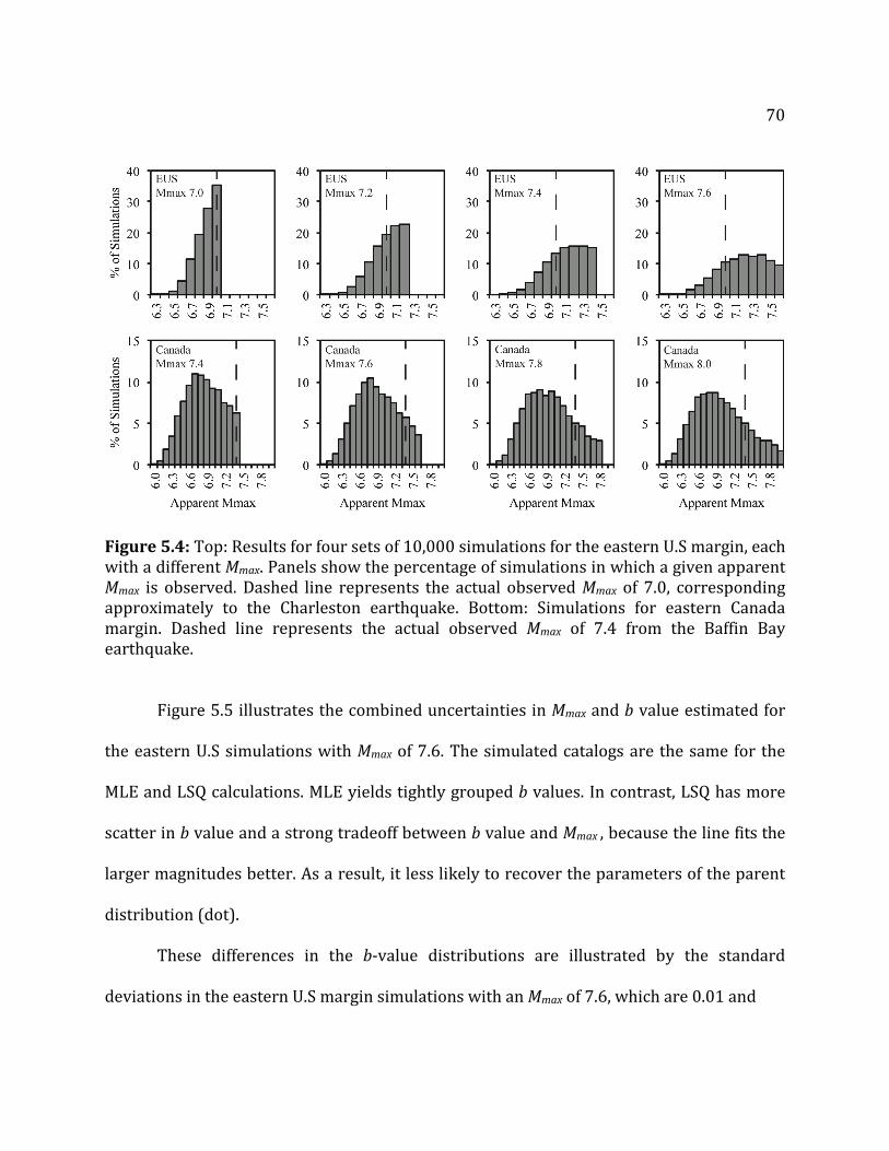
70
Figure 5.4: Top: Results for four sets of 10,000 simulations for the eastern U.S margin, each
with a different Mmax. Panels show the percentage of simulations in which a given apparent
Mmax is observed. Dashed line represents the actual observed Mmax of 7.0, corresponding
approximately to the Charleston earthquake. Bottom: Simulations for eastern Canada
margin. Dashed line represents the actual observed Mmax of 7.4 from the Baffin Bay
earthquake.
Figure 5.5 illustrates the combined uncertainties in Mmax and b value estimated for
the eastern U.S simulations with Mmax of 7.6. The simulated catalogs are the same for the
MLE and LSQ calculations. MLE yields tightly grouped b values. In contrast, LSQ has more
scatter in b value and a strong tradeoff between b value and Mmax , because the line fits the
larger magnitudes better. As a result, it less likely to recover the parameters of the parent
distribution (dot).
These differences in the b-value distributions are illustrated by the standard
deviations in the eastern U.S margin simulations with an Mmax of 7.6, which are 0.01 and
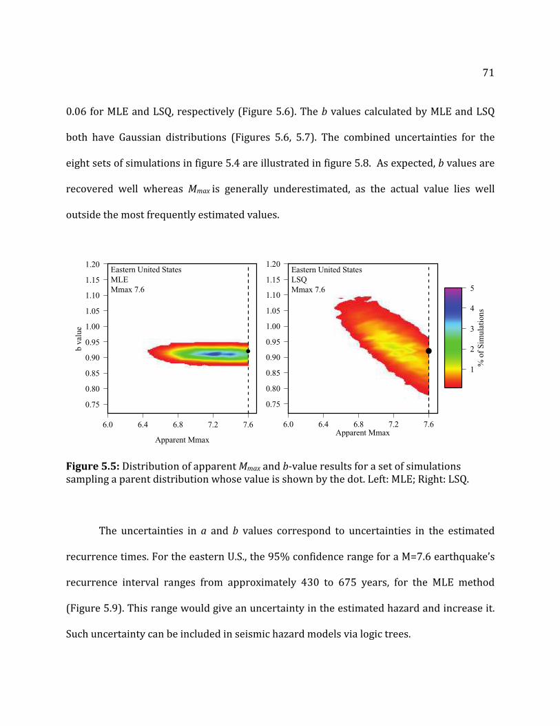
71
0.06 for MLE and LSQ, respectively (Figure 5.6). The b values calculated by MLE and LSQ
both have Gaussian distributions (Figures 5.6, 5.7). The combined uncertainties for the
eight sets of simulations in figure 5.4 are illustrated in figure 5.8. As expected, b values are
recovered well whereas Mmax is generally underestimated, as the actual value lies well
outside the most frequently estimated values.
Figure 5.5: Distribution of apparent Mmax and b-value results for a set of simulations
sampling a parent distribution whose value is shown by the dot. Left: MLE; Right: LSQ.
The uncertainties in a and b values correspond to uncertainties in the estimated
recurrence times. For the eastern U.S., the 95% confidence range for a M=7.6 earthquake’s
recurrence interval ranges from approximately 430 to 675 years, for the MLE method
(Figure 5.9). This range would give an uncertainty in the estimated hazard and increase it.
Such uncertainty can be included in seismic hazard models via logic trees.
0.75
0.80
0.85
0.90
0.95
1.00
1.05
1.10
1.15
1.20
6.0 6.4 6.8 7.2 7.6Apparent Mmax
1
2
3
4
5
% o
f Si
mul
atio
ns
0.75
0.80
0.85
0.90
0.95
1.00
1.05
1.10
1.15
1.20
b va
lue
6.0 6.4 6.8 7.2 7.6
Apparent Mmax
Eastern United StatesMLEMmax 7.6
Eastern United StatesLSQMmax 7.6

72
Figure 5.6: b-value results for the four sets of 10,000 simulations for the eastern U.S
margin, each with a different Mmax and a=4.24, b=0.92 Top: Panels show the percentage of
simulations in which a given b value, calculated by the MLE method, is observed. Bottom:
Results using the LSQ method to calculate b values.
Figure 5.7: b-value results for the four sets of 10,000 simulations for the eastern Canada
margin, each with a different Mmax and a=4.44, b=0.94. Top: Percentage of simulations in
which a given b value, calculated by the MLE method, is observed. Bottom: Results using
the LSQ method to calculate b values.

73
Figure 5.8: Distributions of MLE estimates for the eight sets of simulations in figure 5.4. As
expected, b values are recovered well whereas Mmax is generally underestimated. Dot
indicates parent distribution parameters.
Figure 5.9: Recurrence time distribution for a M=7.6 earthquake in the eastern U.S.
corresponding to the results of simulations with an Mmax of 7.6. Left: MLE; Right: LSQ.
Dashed line is the parent distribution average value of 565 years.
0
5
10
15
20
25
0 30
0 60
0 90
0 12
00
1500
18
00
2100
24
00
2700
30
00
3300
36
00
% o
f S
imul
atio
ns
Recurrence Time
% o
f S
imul
atio
ns
0
5
10
15
20
325
375
425
475
525
575
625
675
725
775
825
% o
f Si
mul
atio
ns
Recurrence Time
EUSM = 7.6MLE
EUSM = 7.6LSQ

74
5.4 Lower Rhine Embayment Seismic Zone Results
I also briefly examined these issues for the LRE (Figure 5.10). I simulate histories for
Mmax= 6.2, 6.5, 6.8, and 7.1 that are 250,000 years long and are sampled for 700 years, the
period over which the historical seismicity is known for events with M ≥ 5 . Figure 5.11
shows results for the LRE seismic zone for a=2.772 and b=0.942, values calculated by the
Royal Observatory of Belgium by integrating recent and historical seismicity. The MLE
results (Figure 5.12) for the LRE seismic zone have a larger spread than the U.S. margin
because the smaller number of M ≥ 4.0 earthquakes, ~70 versus ~1100, which makes the
MLE results less stable. The most common Mmax value “observed” is 6.0. This case differs
from the eastern North America scenarios in that the simulations’ observed Mmax is likely
larger than the largest earthquake in the historical catalog (M5.7). For example, 78% of the
simulations with an Mmax of 7.1 yield an apparent Mmax greater than M5.7 (Table 5.1).
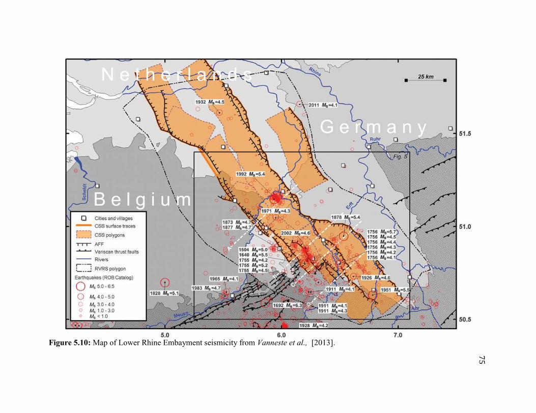
75
Figure 5.10: Map of Lower Rhine Embayment seismicity from Vanneste et al., [2013].

76
Figure 5.11: Results for four sets of 10,000 simulations for the Lower Rhine Embayment
seismic zone, each with a different Mmax. Panels show the percentage of simulations in
which a given apparent Mmax is observed. Dashed line represents the actual observed Mmax
of 5.7, corresponding to the 1756 Düren earthquake.
Figure 5.12: b-value results for the four sets of 10,000 simulations for the Lower Rhine
Embayment, each with a different Mmax and a=4.44, b=0.94. Top: Percentage of simulations
in which a given b value, calculated by the MLE method, is observed. Bottom: Results using
the LSQ method to calculate b values.
0
5
10
15
20
5.0
5.3
5.6
5.9
6.2
6.5
6.8
7.1
% o
f Si
mul
atio
ns
Apparent Mmax
0
5
10
15
20
5.0
5.3
5.6
5.9
6.2
6.5
6.8
7.1
% o
f Si
mul
atio
ns
Apparent Mmax
LREMmax 7.1
LREMmax 6.8
0
5
10
15
20
5.0
5.3
5.6
5.9
6.2
6.5
6.8
7.1
% o
f Si
mul
atio
ns
Apparent Mmax
LREMmax 6.5
% o
f S i
mu l
atio
ns
0
5
10
15
20
5.0
5.3
5.6
5.9
6.2
6.5
6.8
7.1
% o
f Si
mul
atio
ns
Apparent Mmax
LREMmax 6.2
0
10
20
30
0.40
0.
55
0.70
0.
85
1.00
1.
15
1.30
1.
45
1.60
% o
f Si
mul
atio
ns
b value
0
10
20
30
0.40
0.
55
0.70
0.
85
1.00
1.
15
1.30
1.
45
1.60
% o
f Si
mul
atio
ns
b value
0
10
20
30
0.40
0.
55
0.70
0.
85
1.00
1.
15
1.30
1.
45
1.60
% o
f Si
mul
atio
ns
b value
0
5
10
15
20 0.
40
0.55
0.
70
0.85
1.
00
1.15
1.
30
1.45
1.
60
% o
f Si
mul
atio
ns
b value
0
5
10
15
20
0.40
0.
55
0.70
0.
85
1.00
1.
15
1.30
1.
45
1.60
% o
f Si
mul
atio
ns
b value
0
5
10
15
20
0.40
0.
55
0.70
0.
85
1.00
1.
15
1.30
1.
45
1.60
% o
f Si
mul
atio
ns
b value
LRE, Mmax
6.5 LRE, Mmax
6.8 LRE, Mmax
7.1
b = 0.90 ± 0.07 b = 0.90 ± 0.07 b = 0.90 ± 0.07
b = 0.97 ± 0.15 b = 0.94 ± 0.16 b = 0.92 ± 0.17
0
10
20
30
0.40
0.
55
0.70
0.
85
1.00
1.
15
1.30
1.
45
1.60
% o
f Si
mul
atio
ns
b value
% o
f Si
mul
atio
n ss
b value
0
5
10
15
20
0.40
0.
55
0.70
0.
85
1.00
1.
15
1.30
1.
45
1.60
% o
f Si
mul
atio
ns
b value
LRE, Mmax
6.2
b = 1.02 ± 0.13
b = 0.90 ± 0.07

77
Mmax 6.2 Mmax 6.5 Mmax 6.8 Mmax 7.1 Percent of
simulations with observed Mmax >
M5.7
65% 73% 75% 78%
Table 5.1: Percent of simulations with differing Mmax that have apparent maximum
magnitudes above the 1756 Düren earthquake (M5.7).
5.5 Discussion
The simulations suggest that future earthquakes along both margins may be larger
than observed to date. Mmax for both margins may be the same, although if the higher
seismicity in Canada is real rather than a sampling artifact, large events would be more
common there. A complexity is that some of the higher Canadian seismicity rate may reflect
aftershocks of the two recent large earthquakes or of prehistoric earthquakes [Basham and
Adams, 1983; Wolin et al., 2012).
More generally, these simulations demonstrate that Mmax cannot be reliably
estimated from earthquake catalogs. The largest earthquake observed likely reflects the
length of the history used, even if larger earthquakes occur (Figure 5.13). Although the
precise fraction depends on the distribution of recurrence times, a catalog shorter than an
earthquake’s mean recurrence time is likely to not contain an event of that size.
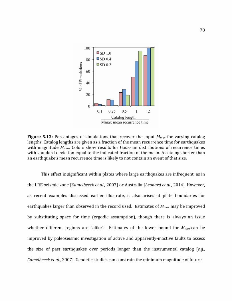
78
Figure 5.13: Percentages of simulations that recover the input Mmax for varying catalog
lengths. Catalog lengths are given as a fraction of the mean recurrence time for earthquakes
with magnitude Mmax. Colors show results for Gaussian distributions of recurrence times
with standard deviation equal to the indicated fraction of the mean. A catalog shorter than
an earthquake’s mean recurrence time is likely to not contain an event of that size.
This effect is significant within plates where large earthquakes are infrequent, as in
the LRE seismic zone [Camelbeeck et al., 2007] or Australia [Leonard et al., 2014]. However,
as recent examples discussed earlier illustrate, it also arises at plate boundaries for
earthquakes larger than observed in the record used. Estimates of Mmax may be improved
by substituting space for time (ergodic assumption), though there is always an issue
whether different regions are “alike”. Estimates of the lower bound for Mmax can be
improved by paleoseismic investigation of active and apparently-inactive faults to assess
the size of past earthquakes over periods longer than the instrumental catalog [e.g.,
Camelbeeck et al., 2007]. Geodetic studies can constrain the minimum magnitude of future
0
20
40
60
80
100
0.1 0.25 0.5 1 2
% o
f Si
mul
atio
ns
Catalog lengthMmax mean recurrence time
SD 1.0
SD 0.4 SD 0.2

79
earthquakes from the strain accumulation rate and time since the last large earthquake
[Manaker et al., 2008]. However, there is no reliable way to infer an upper bound, although
various plausible assumptions can be made. Thus the only certainty about Mmax, is that is at
least as large as that observed to date, as in the adage “anything that did happen, can
happen.”

80
CHAPTER 6
Mantle flow beneath Arabia offset from the opening Red Sea

81
6.1 Introduction
The primary question about continental rifting is the chicken�and�egg issue of how
mantle flow and lithospheric extension are related. The initiation of rifting can be described by
end member models of either active rifting initiated by hot mantle material upwelling below a
continent and weakening it, or passive rifting initiated by stresses within the lithosphere due in
most cases to plate motions that thin the continent, causing mantle upwelling and volcanism
[Sengör and Burke, 1978]. The combined effects of these processes, whose sequence and relative
roles are unclear and likely vary between rifts, sometimes cause rifting to progress from
stretching and faulting the continental lithosphere to active seafloor spreading.
The relative roles of active and passive rifting are hard to resolve because they are
ongoing today in only a few places. The best examples are associated with the rifting of Arabia
from Africa (Figure 6.1). During the past 30 Ma, Arabia’s motion away from Nubia (West
Africa) and Somalia (East Africa) formed the Red Sea and Gulf of Aden [Le Pichon and
Gaulier, 1988; Bosworth et al., 2005; Garfunkel and Beyth, 2006]. The spreading centers in
these young ocean basins, together with the East African rift, are the arms of the Afar triple
junction. This system appears to have evolved as a result of a major episode of magmatism and
uplift beginning about 30–40 Ma that is interpreted as the beginning of the Afar hotspot [Ebinger
and Sleep, 1998; Courtillot et al., 1999] and forces due to the subduction of the Tethyan ocean
lithosphere beneath Eurasia that is presently closing the Persian Gulf [McQuarrie et al., 2003].
Two arms present a consistent picture between lithospheric extension, volcanism, and
mantle flow. The Ethiopia arm is undergoing continental extension and volcanism, underlain by

82
Figure 6.1: Tectonics of the Nubia�Arabia�Somalia three�plate system showing relative and absolute plate motions [ArRajehi et al., 2010], locations of volcanism and dikes [Dixon et al., 1989; Camp and Roobol, 1992], and selected focal mechanisms from CMT catalog.
83
low velocity � presumably hot � material [Debayle et al., 2001]. Shear�wave splitting data
[Gashawbeza et al., 2004] show the fast direction parallel to the rift, consistent with mantle flow
along it. The Gulf of Aden arm shows seafloor spreading, recorded by the magnetic anomalies in
crust formed at the spreading center, along its entire length [Cochran, 1982].
However, the Red Sea arm is more complicated. Seafloor magnetic anomalies and normal
faulting earthquakes typically associated with slow spreading ridges occur almost exclusively
south of 21°N where a deep axial trough is present [Chu and Gordon, 1998; Cochran and
Karner, 2007]. To the north, only a few isolated anomalies are identified, and the sea is floored
by rotated fault blocks. Thus the northern area is interpreted as continental crust being stretched
and faulted with only minor volcanic activity, whereas the southern area has evolved to the point
that new lithosphere is being produced at a spreading axis. This situation has been viewed as
transient until the extension in the northern area evolves into seafloor spreading. This model is
consistent with magnetic and GPS data showing that the rate of opening decreases from about 18
mm/yr at 16°N to about 10 mm/yr at 26°N [Chu and Gordon, 1998; ArRajehi et al., 2010].
6.2 Tomographic Image
Co-workers and I investigated this transition using a seismic tomographic image of
velocity structure, made by Sung-Joon Chang, beneath Arabia and surroundings derived by joint
inversion of a compilation of data. The compilation includes global and regional data sets of
arrival times, body wave waveforms, regional multimode S and surface wave trains, surface
wave group velocities, and constraints on Moho depth from active source seismic studies, gravity
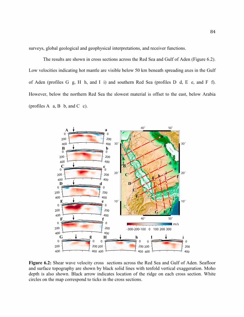
84
surveys, global geological and geophysical interpretations, and receiver functions.
The results are shown in cross sections across the Red Sea and Gulf of Aden (Figure 6.2).
Low velocities indicating hot mantle are visible below 50 km beneath spreading axes in the Gulf
of Aden (profiles G�g, H�h, and I�i) and southern Red Sea (profiles D�d, E�e, and F�f).
However, below the northern Red Sea the slowest material is offset to the east, below Arabia
(profiles A�a, B�b, and C�c).
Figure 6.2: Shear wave velocity cross�sections across the Red Sea and Gulf of Aden. Seafloor and surface topography are shown by black solid lines with tenfold vertical exaggeration. Moho depth is also shown. Black arrow indicates location of the ridge on each cross section. White circles on the map correspond to ticks in the cross sections.

85
This difference is illustrated by an image at 150 km (Figure 6.3). Low velocities occur
beneath the Gulf of Aden and southern Red Sea. However, the lowest velocity material beneath
the southern Red Sea does not extend northwestward below the Red Sea, but instead forms a
channel trending northward beneath Arabia. Shear wave splitting directions show northward
flow parallel to the channel rather than to the Red Sea [Hansen et al., 2006; Sebai et al., 2006].
The upper�mantle low�velocity region has been imaged, first as a broad zone and then
as a channel, in successive earlier regional studies with progressively increasing resolution
[Hadiouche and Zurn, 1992; Debayle et al., 2001; Pasyanos and Nyblade, 2007; Sicilia et al.,
2008]. The dataset Sung-Joon and coworkers used to create the tomographic image combines
much of the data used in these studies in a joint inversion. The resulting improved resolution
shows that the low velocity channel is shallow (extending from 100–300 km), narrow (less than
500 km wide), and displaced eastward rather than extending under the northern Red Sea. This
geometry supports the earlier interpretation of northward flow in the mid upper�mantle from the
Afar hotspot [Park et al., 2008], but shows that the channel is offset from the northern Red Sea
and hence does not represent mantle flow along the Red Sea. Resolution tests in the auxiliary
material show that the low�velocity region is a narrow channel rather than a broad regional
anomaly, and that this channel occurs below Arabia rather than the northern Red Sea.
6.3 Tectonic Interpretation
The geometry of the low velocity anomaly and the shear wave splitting directions jointly
favor their being due to mantle flow, as observed elsewhere [Russo et al., 2010]. However, this

86
geometry differs from cases in which the splitting directions can be interpreted as mantle flow
driven by absolute plate motions [Silver, 1996], because Arabia’s SW�NE absolute motion does
not match the N�S flow and splitting directions. The narrowness of the velocity anomaly and its
depth extent preclude its being due to lithospheric thickness [Rychert and Shearer, 2009].
Figure 6.3: Shear wave velocity map at 150 km depth, showing perturbations relative to reference velocity. Shear wave splitting data are from Gashawbeza et al. [2004] and Hansen et
87al. [2006].
The new data also suggest how the flow may have evolved. Prior to the availability of
tomographic data, the presence of upwelling mantle beneath Arabia was proposed based on the
presence of elevated topography and 20–30 Ma volcanism and dike swarms trending parallel to
the Red Sea but up to several hundred km eastward [Dixon et al., 1989]. Because little uplift and
volcanism occur on the west side of the Red Sea, the asymmetric volcanism and uplift were
hypothesized to reflect the initial location of upwelling that caused the Red Sea rifting as Arabia
migrated northeastward over the upwelling which was assumed to be fixed in the mantle.
However, the tomographic data show that the hot mantle flow is not beneath the Red Sea.
Instead, it occurs beneath the loci of two distinct phases of volcanism in western Arabia. As
previously observed [Camp and Roobol, 1992], the older (pre�15 Ma) northwest�trending
volcanism and younger north�trending volcanism that continues to the present, overlap with
different trends. Thus I hypothesize that the flow from the fixed or slow�moving hotspot forms a
channel that has lengthened with time and been deflected by Arabia’s northeastward absolute
motion, such that it remains below Arabia but rotated to a more north�south trend consistent
with that of the younger volcanics. Figure 6.4 shows such a scenario, in which present plate
motions are used throughout because their detailed history is not well known. The deflection is
favored by the fact that Arabia’s absolute motion is almost perpendicular to the Red Sea.
Analogous deflection of upwelling mantle by absolute plate motion has been proposed for the
Eifel hotspot [Walker et al., 2007].
This model is schematic in several ways. The channel geometry is reasonably but not

88perfectly resolved. A similar direction of anisotropy is observed east of the channel, where
Figure 6.4: (Top) Schematic model for the evolution of the low velocity channel, assuming flow from a fixed hotspot has been deflected by Arabia’s northeastward absolute motion. (Bottom) Possible future geometries in which (Left) extension in the northern Red Sea develops into seafloor spreading or ceases as rifting develops within Arabia along the low velocity channel and (Right) progresses to seafloor spreading.
lithosphere is thicker [Stern and Johnson, 2010], consistent with the view that anisotropy can
arise from both mantle flow and lithospheric structure [Hansen et al., 2006]. Not all volcanism is

89directly above the channel, presumably because the locations of volcanism also reflect
structures
in the lithosphere or due to ongoing opening of the Red Sea. Most intriguingly, the volcanism
occurred in pulses rather than continuously. However, the model offers a general explanation for
the persistence of volcanism with changing trend above the channel’s current location. It is
consistent with geochemical data [Camp and Roobol, 1992; Krienitz et al., 2009] interpreted as
showing that the Arabian volcanics reflect melting that progressed northward and involved a
plume source.
This geometry may have evolved as flow from the hotspot was channeled by the
pre�rifting structure of the base of the lithosphere [Ebinger and Sleep, 1998] and may still be
affected by lithospheric structure. In particular, Cenozoic volcanic activity is absent in the Afif
Terrane that contains some of the oldest crust in the Arabian Shield, of Paleoproterozoic age, but
present to the west [Stoeser and Frost, 2006]. Similarly, the locus of rifting may have been
controlled by preexisting weakness in the continental lithosphere [Dixon et al., 1989; Cloetingh
et al., 1995].
This situation shows aspects of both active and passive rifting models, and could remain
as is or evolve in either direction (Figure 6.4). There is no reason to believe that active sea floor
spreading will begin soon in the northern Red Sea, because the hot mantle flow remains to the
east. The present regime of extension in the north seems stable, as also suggested by the
basement fault geometry [Cochran and Karner, 2007]. It could eventually evolve into sea floor
spreading, in which case the mantle flow should be deflected to the northern Red Sea, as
90observed below the Gulf of Aden. At present this seems not to be occurring, given the
shear�wave splitting data. Alternatively, active rifting could evolve in Arabia above the channel,
given that some extension occurs along the active volcanic trend [Camp and Roobol, 1992;
Pallister et
al., 2010]. Ultimately, the northern Red Sea rift could be abandoned. This “re-rifting” situation
would be similar those observed in the North Atlantic, where volcanism associated with hotspots
produced renewed continental rifting that eventually developed into new seafloor spreading axes
[Skogseid et al., 2000; Mu�ller et al., 2001].
Arabia and its surroundings thus illustrate how many complexities of the rifting process
observed in the geological record [Corti et al., 2003; Huismans and Beaumont, 2003] can arise.
The order, timing, magnitude, and locations of volcanism and extension have varied during
rifting, as shown by the fact that the East Africa rift has considerable volcanism and little
extension, whereas the Gulf of Aden has less volcanism but more extension. The fact that in the
Red Sea and Arabia a situation with aspects of both active and passive rifting occurs and seems
stable for some time illustrates that lithospheric extension and mantle flow can act somewhat
independently in different places for a long time before coalescing to seafloor spreading.
91
Chapter 7
Mapping sediment thickness in Minnesota with horizontal-to-vertical spectral ratios from
USArray data

92
7.1 Introduction
The spectral ratio of seismic noise recorded on the horizontal and vertical components of
a seismometer (HVSR) has been shown to be an inexpensive and useful tool for characterizing
near-surface structure [Nakamura, 1989]. When sediments with low shear wave velocity overlie
higher-velocity bedrock, the HVSR typically has a pronounced peak at the fundamental resonant
frequency fr of the sediment layer fr = V s / 4h, where V s is the average shear wave velocity in
the layer and h is the layer thickness.
As a result, HVSR studies can be used to estimate the fundamental frequency for
earthquake engineering applications [Bindi et al., 2000]. The HVSR can also be used to infer the
layer thickness and thus depth to bedrock. Because the inferred depths are in good agreement
with those measured directly in boreholes [Ibs-von Seht and Wohlenberg, 1999; Parolai et al.,
2002; Nguyen et al., 2004; Chandler and Lively, 2011], HVSR studies can be used to infer
basement depths in areas with few borehole sites [Lane et al., 2008].
Lachet and Bard [1994] show that HVSR peaks have the following properties: the peak
frequencies are independent of the source excitation function and the amplitude of the peak is
related to the velocity contrast at the rock-sediment interface and the Poisson’s ratio of the
93sediment. Thus this technique gives best results where sediments have a high impedance
contrast, a factor of two or more, with the bedrock.
The origin of the HVSR peak remains under discussion. Some researchers suggest the
HVSR peak is due to fundamental mode Rayleigh waves [Lachet and Bard, 1994; Konno and
Ohmachi, 1998], while others explain the HVSR peak as resulting from vertically incident SH
waves [Nakamura, 2000]. As a result, although the resonance frequency of sedimentary sites
seems to be well estimated by the method, it remains unclear how to use the peak amplitude to
infer site amplification at this frequency.
Typically, HVSR studies are conducted by moving a few, often one, seismometers from
site to site and collecting short samples of data. In contrast, USArray provides the opportunity
for analogous studies using a network spanning a large area that can provide long lengths of data.
7.2 Data
Minnesota was chosen as the study area because Chandler and Lively [2011] have
obtained good HVSR results with short seismic records, prompting me to explore application of
the longer records at sites available from USArray data. Most of the state is covered by
sediments from the past recent glaciation, which are thought to have a high impedance contrast
with the bedrock. Sediment thickness values are available from work by the Minnesota
Geological Survey [Jirsa et al., 2010], which provides a mapped surface created from an
irregularly spaced grid of well data.
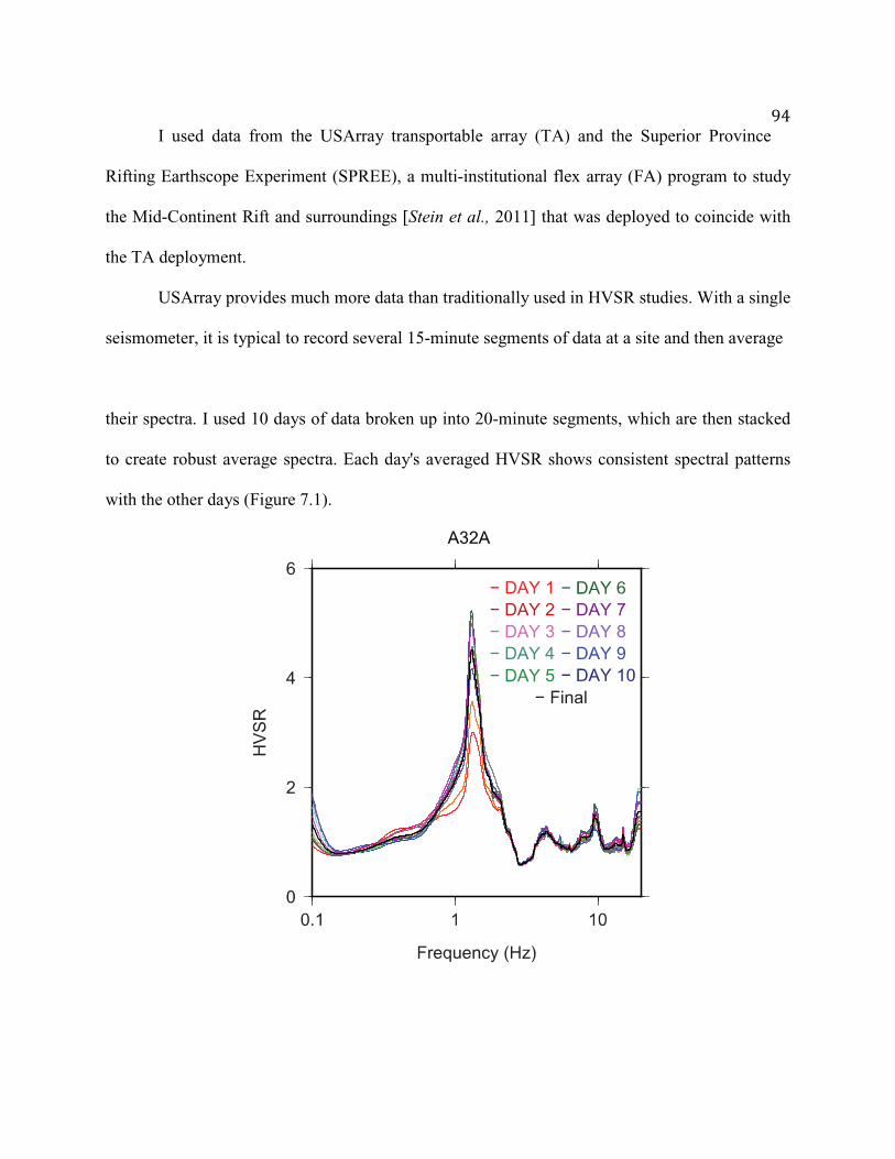
94 I used data from the USArray transportable array (TA) and the Superior Province
Rifting Earthscope Experiment (SPREE), a multi-institutional flex array (FA) program to study
the Mid-Continent Rift and surroundings [Stein et al., 2011] that was deployed to coincide with
the TA deployment.
USArray provides much more data than traditionally used in HVSR studies. With a single
seismometer, it is typical to record several 15-minute segments of data at a site and then average
their spectra. I used 10 days of data broken up into 20-minute segments, which are then stacked
to create robust average spectra. Each day's averaged HVSR shows consistent spectral patterns
with the other days (Figure 7.1).
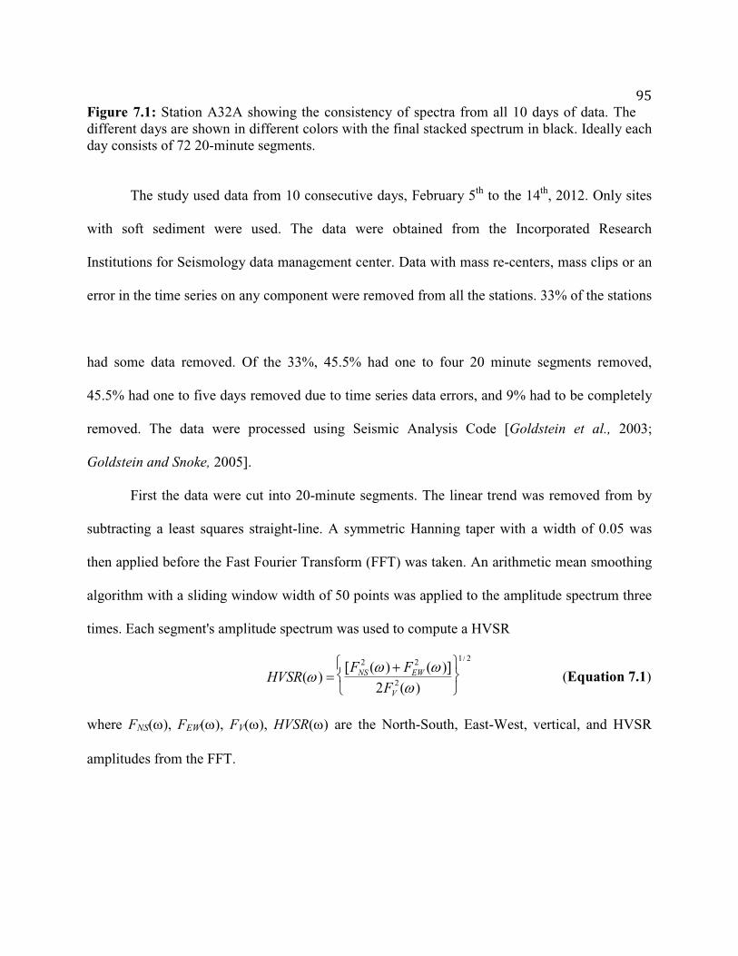
95Figure 7.1: Station A32A showing the consistency of spectra from all 10 days of data. The different days are shown in different colors with the final stacked spectrum in black. Ideally each day consists of 72 20-minute segments.
The study used data from 10 consecutive days, February 5th to the 14th, 2012. Only sites
with soft sediment were used. The data were obtained from the Incorporated Research
Institutions for Seismology data management center. Data with mass re-centers, mass clips or an
error in the time series on any component were removed from all the stations. 33% of the stations
had some data removed. Of the 33%, 45.5% had one to four 20 minute segments removed,
45.5% had one to five days removed due to time series data errors, and 9% had to be completely
removed. The data were processed using Seismic Analysis Code [Goldstein et al., 2003;
Goldstein and Snoke, 2005].
First the data were cut into 20-minute segments. The linear trend was removed from by
subtracting a least squares straight-line. A symmetric Hanning taper with a width of 0.05 was
then applied before the Fast Fourier Transform (FFT) was taken. An arithmetic mean smoothing
algorithm with a sliding window width of 50 points was applied to the amplitude spectrum three
times. Each segment's amplitude spectrum was used to compute a HVSR
HVSR(ω ) =[FNS
2 (ω ) + FEW2 (ω )]
2FV2(ω )
1/ 2
(Equation 7.1)
where FNS(ω), FEW(ω), FV(ω), HVSR(ω) are the North-South, East-West, vertical, and HVSR
amplitudes from the FFT.

96 Every 20-minute HVSR segment for a given station was then averaged to yield the
final HVSR for that station (Table 7.1). The depth of soft sediment at the site was taken from the
Minnesota Geological Survey grid.
Station
Network
Latitude
Longitude
fHVSR (Hz)
AHVSR
hdata (m)
hcalc (m)
Difference (%)
A31A TA 48.93 -97.19 0.80 8.9 63 116 -84 A32A TA 48.92 -96.49 1.32 4.8 110 69 37 A33A TA 48.94 -95.39 2.73 8.0 51 33 35 B32A TA 48.40 -96.54 1.33 8.5 111 69 38 B33A TA 48.27 -95.59 2.02 4.8 73 45 39 B34A TA 48.49 -94.65 1.50 7.0 40 61 -53 B35A TA 48.36 -93.73 3.83 6.4 23 23 2
C32A TA 47.83 -96.53 1.00 9.7 86 93 -8 C33A TA 47.76 -95.77 1.29 6.4 116 71 39 C34A TA 47.65 -94.91 0.75 8.7 127 124 2 C35A TA 47.70 -93.98 2.32 9.5 28 39 -40 C36A TA 47.76 -92.84 6.86 5.6 4 13 -204 C39A TA 47.82 -90.13 7.05 6.9 15 12 18 D33A TA 47.14 -95.84 0.64 8.1 189 146 23 D34A TA 47.09 -95.20 0.57 8.4 133 167 -25 D35A TA 47.08 -94.05 1.48 7.7 34 62 -80 D36A TA 47.18 -93.16 1.87 7.2 97 48 50 E33A TA 46.50 -96.01 0.84 8.8 148 110 25 E34A TA 46.51 -95.17 0.84 4.5 100 110 -10 E35A TA 46.56 -94.40 1.29 5.5 69 71 -3 E36A TA 46.52 -93.26 1.72 4.2 18 53 -185 F33A TA 45.84 -96.29 2.07 5.4 42 43 -4 F34A TA 45.80 -95.26 1.52 4.4 93 60 36 F35A TA 45.86 -94.57 1.39 7.4 56 66 -17 F36A TA 45.86 -93.52 6.07 7.2 27 14 47 G33A TA 45.19 -96.44 1.83 4.7 39 49 -28 G34A TA 45.24 -95.64 1.18 5.4 55 78 -41 G35A TA 45.22 -94.49 1.26 7.3 90 73 19 G36A TA 45.23 -93.75 1.70 6.3 111 53 52 H34A TA 44.67 -95.78 1.46 6.1 53 62 -18 H35A TA 44.70 -94.83 1.36 7.5 89 67 25 H36A TA 44.58 -93.93 0.78 4.9 164 119 27 H37A TA 44.58 -92.92 2.22 5.9 44 40 8

97I34A TA 44.04 -95.86 1.01 5.4 80 92 -15 I35A TA 43.86 -94.98 0.84 8.5 95 110 -16 I36A TA 44.02 -94.01 1.07 7.4 90 86 4 I37A TA 44.01 -93.40 2.62 4.6 30 34 -12 I38A TA 44.04 -92.33 14.06 5.0 3 6 -94
SM23 SPREE 46.03 -92.37 3.12 3.5 25 28 -12 SM24 SPREE 45.99 -92.54 4.19 6.4 11 21 -83 SM31 SPREE 45.35 -92.75 1.43 5.0 60 64 -7 SM32 SPREE 45.27 -92.83 3.24 6.6 37 27 26 SM33 SPREE 44.67 -93.48 0.94 6.5 114 99 13 SM34 SPREE 44.67 -93.48 1.09 4.8 125 84 33 SM36 SPREE 44.46 -93.39 2.43 6.7 46 37 19 SM39 SPREE 44.05 -93.20 2.51 4.4 37 36 5 SM40 SPREE 43.91 -93.10 2.49 4.5 34 36 -7 SM41 SPREE 43.77 -93.08 2.96 7.7 30 30 1 SM42 SPREE 43.63 -93.05 2.76 6.0 11 32 -197 SN43 SPREE 46.75 -93.21 1.59 5.2 42 57 -36
SN44 SPREE 46.72 -93.13 2.30 5.8 63 39 39 SN45 SPREE 46.66 -93.04 1.75 4.2 57 52 10 SN46 SPREE 46.61 -92.92 2.04 5.5 49 44 9 SN47 SPREE 46.53 -92.83 16.35 4.0 13 5 61 SN48 SPREE 46.45 -92.69 0.61 6.5 184 153 17 SS65 SPREE 44.02 -94.80 1.70 4.5 29 53 -84 SS66 SPREE 44.02 -94.80 1.35 5.4 30 68 -124 SS68 SPREE 44.06 -93.89 1.46 6.9 62 63 -1 SS69 SPREE 44.03 -93.74 1.95 3.4 76 46 39 SS70 SPREE 44.01 -93.64 1.34 6.6 62 68 -9 SS72 SPREE 44.04 -93.27 3.02 4.3 27 29 -9 SS73 SPREE 44.03 -93.14 2.08 6.9 45 43 4 SS74 SPREE 44.03 -93.00 2.65 8.5 54 34 38 SS75 SPREE 44.04 -92.88 4.72 5.7 19 18 4 SS76 SPREE 44.03 -92.74 11.47 5.1 11 7 32 SS77 SPREE 44.02 -92.59 2.47 4.8 29 36 -24 SS78 SPREE 43.97 -92.38 3.89 6.8 17 23 -36
Table 7.1: fHVSR = HVSR peak frequency; AHVSR = Amplitude of HVSR peak; hdata = Depth of soft sediment from Minnesota Geological Survey; hcalc = calculated soft sediment thickness from regression fit (equation 7.3); Difference % = [(hdata - hcalc)/hdata] x 100

98 The data quality varies by location and network. Thicker sediments generally yield
narrower HVSR peaks. Only one station in the TA network did not show a coherent HVSR peak,
while eight SPREE stations were discarded due to poor HVSR peaks.
I examined whether the peaks resulted from a high horizontal component, a low vertical
component, or both. 48% of the SPREE stations have both a low vertical, and high horizontal
component, compared to 79% of TA stations (Figure 7.2). However, I found no obvious spatial
patterns in which components caused the peak (Figure 7.3).
7.3 Results
The HVSR peak frequencies show a consistent pattern throughout Minnesota (Figure
7.3). Following Ibs-von Seht and Wohlenberg [1999], I assumed that the HVSR peak frequency
fHVSR is related to the soft sediment thickness h in meters at each site by
h = afHVSRb
(Equation 7.2)
The constants a and b were estimated by taking the logarithm and computing a linear
regression, yielding
h = 91.95 f HVSR−1.029 (Equation 7.3)
The regression fits the data well, yielding a R2 of 0.74 (Figure 7.4). Both networks fit about
equally well by the regression curve. Given that the SPREE sites are in a limited area, this
implies that sediment properties are similar across the region, making a single curve fit better.

99Encouragingly my regression results are similar to those obtained by Chandler and Lively
[2011], which use different sites and surveying methods.
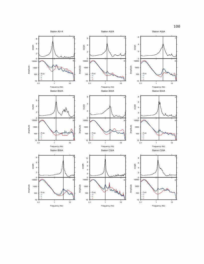
100
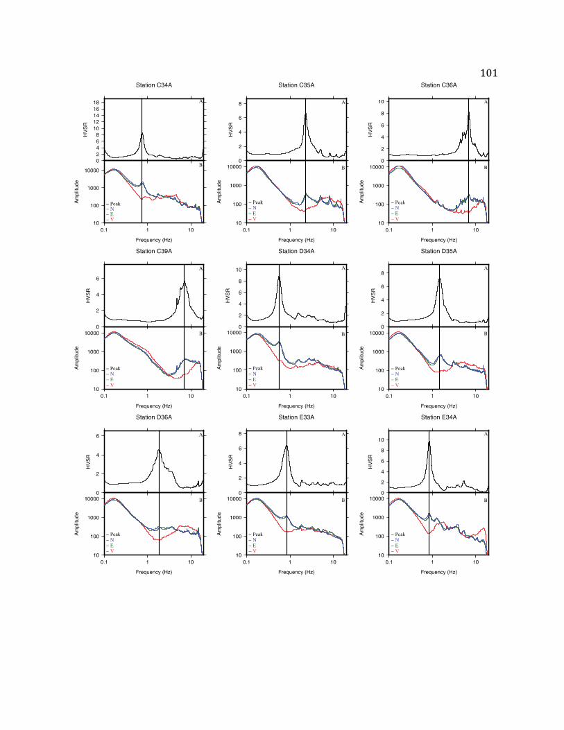
101

102
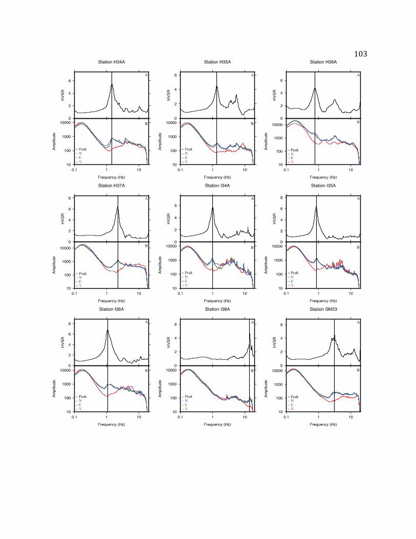
103
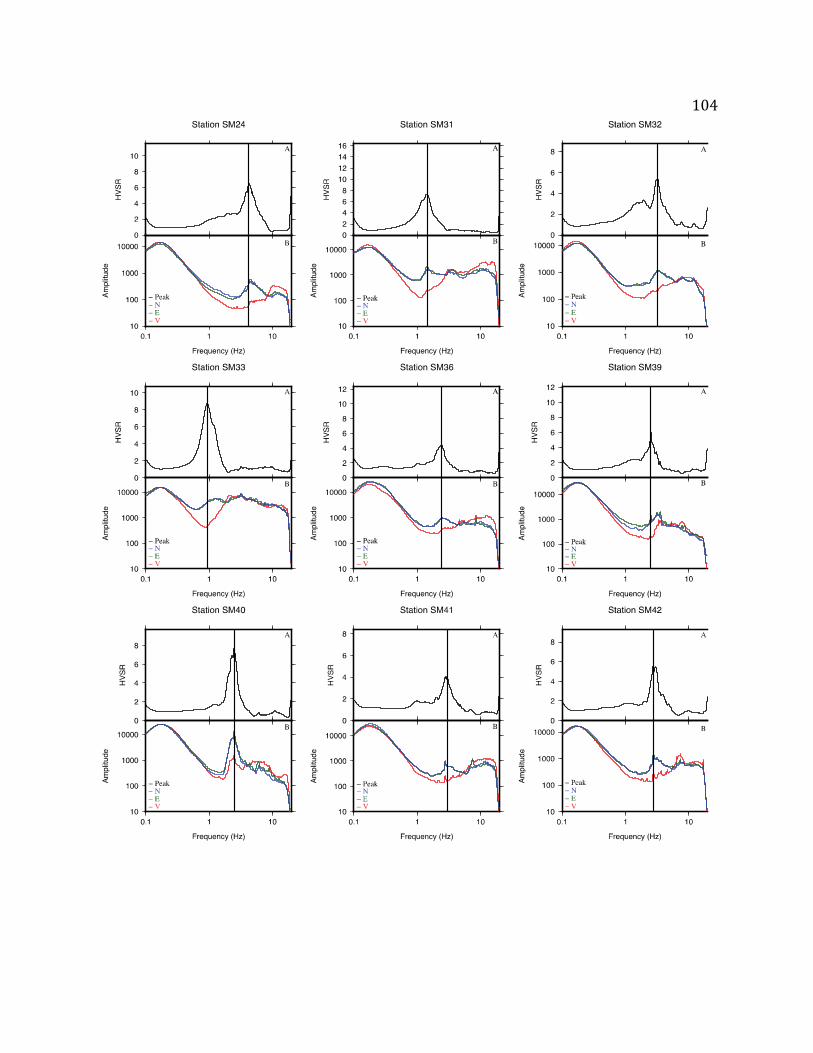
104

105

106
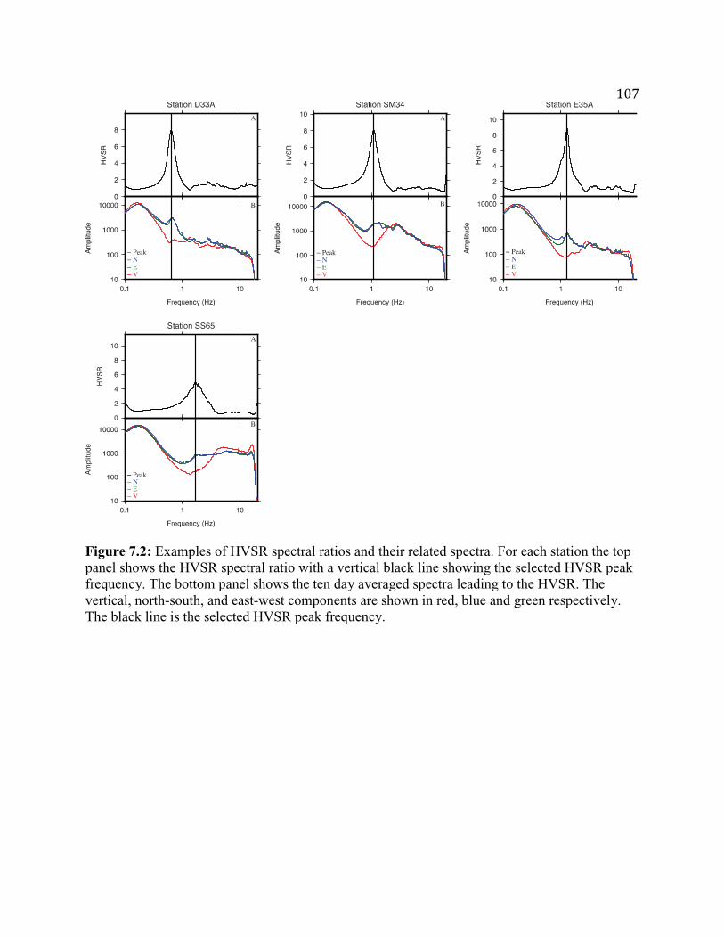
107
Figure 7.2: Examples of HVSR spectral ratios and their related spectra. For each station the top panel shows the HVSR spectral ratio with a vertical black line showing the selected HVSR peak frequency. The bottom panel shows the ten day averaged spectra leading to the HVSR. The vertical, north-south, and east-west components are shown in red, blue and green respectively. The black line is the selected HVSR peak frequency.

108
Figure 7.3: HVSR peak frequency map showing a smooth trend across the study area. Black squares are stations with both a low vertical component and a high horizontal component. Inverted triangles have only a low vertical component. Triangles have only high horizontal components. Which components contribute to the peak has no general pattern.
0 100 200
km
0
2
4
6
8
10
12
14
16
180 100 200
km
HV
SR
pea
k fr
eque
ncy
(Hz)

109
Figure 7.4: A) Data and best fit for the relation between peak frequency and sediment thickness. Orange line is Chandler and Lively [2011] relation, and the black line is this study. Blue dots are TA stations, green dots are SPREE stations. The two networks give similar results. B) Data and best fit for Iowa TA sites. Red dots are TA stations.
I also conducted a similar study for Iowa using the TA sites there and sediment thickness
values from the Iowa Geological Survey [Witzke et al., 2010], I found that the scatter was
significantly greater, shown by a R2 of 0.49 (Figure 7.4B). This is probably due to the sediment
to bedrock contrast being less strong and sediment properties being more laterally variable,
presumably because not all of Iowa was recently glaciated.
0
20
40
60
80
100
120
140
160
180
200
0 2 4 6 8 10 12 14 16 18 20
Sof
t sed
imen
t thi
ckne
ss (
m)
HVSR peak frequency (Hz)
0
20
40
60
80
100
120
140
160
180
200
0 2 4 6 8 10 12 14 16 18 20
Sof
t sed
imen
t thi
ckne
ss (
m)
HVSR peak frequency (Hz)
TA
SPREE
Minnesota Iowa
TA A B

110
Figure 7.5: A) Sediment thickness map from taking values at study sites from Minnesota Geological Survey and contouring. B) Sediment thickness map from taking regression curve values at study sites and contouring. Black triangles are TA stations, white triangles are SPREE stations.
The map of sediment thickness for Minnesota inferred from the peak frequencies at each
site using equation 7.3 is similar to one derived from sampling the Minnesota Geological
Survey’s sediment thickness map at the sites (Figure 7.5). The differences are shown by a
histogram and as percentages in figure 7.6. The absolute sediment thickness difference at each
site is reasonable and does not have any clear bias. Not surprisingly, the largest percentage
differences arise for sites with thin sediment.
Soft sediment thickness Calculated soft sediment thickness
A
Met
ers
0
20
40
60
80
100
120
140
160
180
2000 100 200
kmA BBA

111
Figure 7.6: Left: Histogram of differences in sediment thickness at sites between the Minnesota Geological Survey sediment thickness map and thickness inferred from HVSR peak frequencies. Right: Differences shown as percentages as a function of sediment thicknesses. Red and green lines show ±50% and ±25%.
The HVSR method using data from the USArray thus provides good way to estimate the
sediment thickness at sites. This result is consistent with earlier studies that find this to be true
when sediments are similar across a study region and their impedance contrast with the basement
rocks is strong.
-250
-200
-150
-100
-50
0
50
100
0 50 100 150 200
Mis
fit (
%)
Soft sediment thickness (m)
TA
SPREE 0
2
4
6
8
10
12
14
16
18
-60
-50
-40
-30
-20
-10 0 10
20
30
40
50
60
Num
ber
of s
ites
Absolute thickness errors (m)

112CHAPTER 8
Conclusions and Future Work

1138.1 Conclusions and Links
In this dissertation I have presented research in two related fields, the tectonics of rifting
and intraplate seismicity. Chapter 7, which diverges somewhat from this theme, is linked to
Chapters 4 and 5 in that H/V results can be applied to seismic hazard analysis.
In Chapter 2, I modeled gravity data and found that the east arm of the MCR has less
magma than the west arm, and proposed a plausible microplate model that gives an explanation
for why. Chapter 3 extends this analysis by placing the microplate model in the regional plate
tectonic context. It proposes that the MCR formed as part of the separation of Amazonia
(Precambrian northeast South America) from Laurentia (Precambrian North America) and
became inactive once seafloor spreading was established. This new view is important in that
instead of viewing the MCR as an isolated and failed isolated episode of mid-plate volcanism, it
is viewed as part of a successful rifting event forming an integral part of the assembly of
Rodinia.
Chapter 4 looks at a seismically active failed rift system in the interior of a plate. I
examine whether the seismicity supports a modeling prediction that the 1811-1812 earthquakes
transferred stress from the New Madrid seismic zone to the Wabash Valley seismic zone. I
combine historical seismicity catalogs with recent catalogs to define the Gutenberg-Richter
relationship for the two geologically linked regions. I conclude that the seismicity difference is
not indicative of stress transfer to the WVSZ.
Chapter 5 continues the theme of using seismic catalogs, to infer earthquake hazards. I do
so by sampling simulated catalogs to see what parameters can be reliably estimated from the

114short earthquake catalogs available. I find that the b values inferred depend on the method
used to estimate them. In Chapter 4, I used the least squares method to derive the b value. In
Chapter 5, I show that least squares has significantly more scatter than the maximum likelihood
estimate method but is a better description of the data itself. While the total scatter in the b
values is an important result, most of that variation is due to larger earthquakes. The number of
small earthquakes is more stable, which is where the difference in the New Madrid and Wabash
Valley seismic zones arises. Hence the conclusion in Chapter 4 that the New Madrid seismic
zone has more small earthquakes, probably due to being aftershocks of the 1811-1812 events, is
still valid.
The variation in b values inferred for both the MLE and LSQ methods shown in Chapter
5 could have significant impact on hazard modeling. An even more interesting result is that the
observed Mmax for the areas I studied are those most frequently arising in my simulations, rather
than the actual maximum in the simulations. This indicates that we have probably not observed
the largest earthquakes. This method does not predict the largest earthquake in a given region,
but illustrates the need for paleoseismology, ideally a systematic effort looking at both dormant
and active intraplate faults.
Chapter 6 explores rifting in an active system, the Red Sea. I propose a scenario in which
the Red Sea may stop rifting because hot sublithospheric flow causes ‘re-rifting’ in the interior of
Arabia. This possibility is akin to the view in Chapter 3 that the rifting process can lead to much
more complex tectonic evolution than often assumed.

115
8.2 Reflections and Future Work
My research on the tectonics of rifting has sparked many more questions than it has
answered. The MCR scenario that I proposed suggests that many ‘isolated’ intraplate magmatic
events that appear to have “failed,” in that they did not break the continent, were actually part of
successful regional plate reorganizations. A natural extension to chapters 2 and 3 would be to
investigate other isolated and apparently failed rifts to see if they were associated with a
successful rifting event.
In Chapter 2 I modeled the MCR gravity anomalies as a lower crustal intrusion. This
explains the first order effects in the gravity anomalies and is a good way to compare the two rift
arms, but is not a full view of the magma intrusions. A question that interests me is what is the
ratio of lower crustal intrusion to diking events? Furthermore is there a relationship between
deep intrusions and surface extension? Answering these questions would likely need seismic
refraction or reflection data, but could lead to key insights into how magma intrusions and
extension relate. The results could also indicate how rifts subside, and how heat flow evolved
through time in a rift, both of which are important factors in hydrocarbon formation.
The next step for the maximum magnitude studies is to test different methods of
predicting Mmax on simulated catalogs. I also want to use different earthquake simulation
techniques, either a time independent recurrence model or the Epidemic-Type Aftershock
Sequence Model. Understanding how major earthquakes migrate in intraplate zones could
significantly improve seismic hazard models. Paleoseismology could help via a systematic
116
investigation of active and, perhaps more importantly, apparently-inactive faults to gain insight
into how major earthquakes migrate through time.
More broadly this research points to weak points in seismic hazard modeling. The failure
of earthquake hazard maps indicated by the destructive Tohoku, Haiti, and Wenchuan
earthquakes has drawn attention to the fact that we do not know how well seismic hazard models
actually predict shaking over a given period of time? One way to address this would be to
compare the amount of predicted shaking in a given region to the amount of actual shaking in
that region. I think this is a key step in evaluating hazard models that would give us insights
about how to further improve them. Given that long time periods are needed to accumulate
enough real data for this purpose, synthetic catalog experiments are an alternative that can give
valuable insight.

117
References Adams, D. C., and G. R. Keller (1996), Precambrian basement geology of the Permian Basin
region of West Texas and eastern New Mexico: A geophysical perspective, AAPG Bulletin, 80(3), 410-431.
Aki, K. (1965), Maximum likelihood estimate of b in the formula log n=a-bm and its confidence
limits, Bulletin of the Earthquake Research Institute = Tokyo Daigaku Jishin Kenkyusho Iho, 43, Part 2, 237-239.
ArRajehi, A., et al. (2010), Geodetic constraints on present-day motion of the Arabian Plate:
Implications for Red Sea and Gulf of Aden rifting, Tectonics, 29, 10. Basham, P.W and J. Adams (1983). Earthquakes on the continental margin of eastern
Canada--need future large events be confined to the locations of large historical events? in "The 1886 Charleston earthquake and its implications for today," U.S. Geol. Survey Open File Report 83-842, pp. 456-467.
Bassin, C. (2000), The Current Limits of resolution for surface wave tomography in North
America, EOS Trans. AGU. Bear, G. W., J. A. Rupp, and A. J. Rudman (1997), Seismic interpretation of the deep structure
of the Wabash Valley fault system, Seismological Research Letters, 68(4), 624-640. Bedle, H., and S. van der Lee (2009), S velocity variations beneath North America, Journal of
Geophysical Research-Solid Earth, 114. Bell, A., M. Naylor and Ian G. Main (2013), Convergence of the frequency-size distribution of
global earthquakes, Geophysical Research Letters, 40, 2585–2589, doi:10.1002/grl.50416. Bindi, D., S. Parolai, D. Spallarossa, and M. Catteneo (2000), Site effects by H/V ratio:
Comparison of two different procedures, J. Earthqu. Eng., 4(1), 97-113. Blakely, R. J. (1996), Potential theory in gravity and magnetic applications, Cambridge
University Press. Bosworth, W., P. Huchon, and K. McClay (2005), The Red Sea and Gulf of Aden basins, Journal
of African Earth Sciences, 43(1-3), 334-378. Braile, L. W., W. J. Hinze, G. R. Keller, E. G. Lidiak, and J. L. Sexton (1986), Tectonic
Development of the New Madrid Rift Complex, Mississippi Embayment, North-America, Tectonophysics, 131(1-2), 1-21.

118
Brown, L., L. Jensen, J. Oliver, S. Kaufman, and D. Steiner (1982), Rift structure beneath the Michigan Basin from COCORP profiling, Geology, 10(12), 645-649.
Buening, J. D. (2013), An integrated geophysical and geological study of the relationships
between the Grenville orogen and Mid-Continent Rift System, 72 pp, University of Oklahoma.
Camelbeeck, T., K. Vanneste, P. Alexandre, K. Verbeeck, T. Petermans, P. Rosset, M. Everaerts,
R. Warnant, and M. Van Camp (2007), Relevance of active faulting and seismicity studies to assessments of long-term earthquake activity and maximum magnitude in intraplate northwest Europe, between the Lower Rhine Embayment and the North Sea, in Continental Intraplate Earthquakes: Science, Hazard, and Policy Issues, edited by S. Stein and S. Mazzotti, pp. 193-224, Geological Soc Amer Inc, Boulder.
Camp, V. E., and M. J. Roobol (1992), Upwelling Asthenosphere Beneath Western Arabia and
its Regional Implications, Journal of Geophysical Research-Solid Earth, 97(B11), 15255-15271.
Cannon, W. F. (1992), The Midcontinent Rift in the Lake Superior region with emphasis on its
geodynamic evolution, Tectonophysics, 213(1-2), 41-48. Cannon, W. F. (1994), Closing of the Midcontinent Rift – a far-field effect of Grenvillian
compression, Geology, 22(2), 155-158. Cannon, W. F., Z. E. Peterman, and P. K. Sims (1993), Crustal-scale thrusting and origin of the
Montreal River Monocline; a 35-km-thick cross section of the Midcontinent Rift in northern Michigan and Wisconsin, Tectonics, 12(3), 728-744.
Cannon, W. F., et al. (1989), The North American Midcontinent Rift beneath Lake Superior from
GLIMPCE seismic reflection profiling, Tectonics, 8(2), 305-332. Chandler, V., and R. S. Lively (2011), Application of the H/V passive seismic method in
Minnesota: some preliminary insights, Geological Society of America Abstracts with Programs, Vol. 43, No. 5, p. 147, 2011.
Chang, S.-J., M. Merino, S. Van der Lee, S. Stein, and C. A. Stein (2011), Mantle flow beneath
Arabia offset from the opening Red Sea, Geophys. Res. Lett., 38(4), 0-Citation L04301. Chase, C. G., and T. H. Gilmer (1973), Precambrian plate tectonics – midcontinent gravity high,
Earth and Planetary Science Letters, 21(1), 70-78.

119
Chu, D. Z., and R. G. Gordon (1998), Current plate motions across the Red Sea, Geophysical Journal International, 135(2), 313-328.
Clark, D., McPherson, A., and Collins, C. D. N. (2011), Australia’s seismogenic neotectonic
record: a case for heterogeneous intraplate deformation. Geoscience Australia Record 2011/11.
Cloetingh, S., J. D. Vanwees, P. A. Vanderbeek, and G. Spadini (1995), Role of Pre-Rift
Rheology in Kinematic of Extensional Basin Formation – Constraints from Thermomechanical Models of Mediterranean and Intracratonic Basins, Marine and Petroleum Geology, 12(8), 793-807.
Cloetingh, S., F. Beekman, P. A. Ziegler, J. D. Van Wees, and D. Sokoutis (2008), Post-rift
compressional reactivation potential of passive margins and extensional basins, in Nature and Origin of Compression in Passive Margins, edited by H. Johnson, T. G. Dore, R. W. Gatliff, R. W. Holdsworth, E. R. Lundin and J. D. Ritchie, pp. 27-70, Geological Soc Publishing House, Bath.
Cochran, J. R. (1982), The Gulf of Aden – Structure and Evolution of a Young Ocean-Basin and
Continental-Margin – Reply, Journal of Geophysical Research, 87(NB8), 6765-6770. Cochran, J. R., and G. D. Karner (2007), Constraints on the deformation and rupturing of
continental lithosphere of the Red Sea; the transition from rifting to drifting, Geological Society Special Publications, 282, 265-289.
Cornell, C. A. (1968), Engineering seismic risk analysis, Bull. Seismol. Soc. Amer., 58(5), 1583-
1606. Corti, G., J. Van Wijk, M. Bonini, D. Sokoutis, S. Cloetingh, F. Innocenti, and P. Manetti
(2003), Transition from continental break-up to punctiform seafloor spreading: How fast, symmetric and magmatic, Geophys. Res. Lett., 30(12), 4.
Courtillot, V., C. Jaupart, I. Manighetti, P. Tapponnier, and J. Besse (1999), On causal links
between flood basalts and continental breakup, Earth and Planetary Science Letters, 166(3-4), 177-195.
Crone, A. J., P. M. De Martini, M. N. Machette, K. Okumura, and J. R. Prescott (2003),
Paleoseismicity of two historically quiescent faults in Australia: Implications for fault behavior in stable continental regions, Bull. Seismol. Soc. Amer., 93(5), 1913-1934.
D'Agrella, F., E. Tohver, J. O. S. Santos, S. A. Elming, R. I. F. Trindade, I. I. G. Pacca, and M.
C. Geraldes (2008), Direct dating of paleomagnetic results from Precambrian sediments in the
120
Amazon craton: Evidence for Grenvillian emplacement of exotic crust in SE Appalachians of North America, Earth and Planetary Science Letters, 267(1-2), 188-199.
Dalziel, I. W. D., S. Mosher, and L. M. Gahagan (2000), Laurentia-Kalahari collision and the
assembly of Rodinia, Journal of Geology, 108(5), 499-513. Davis, D. W., and J. C. Green (1997), Geochronology of the North American Midcontinent rift
in western Lake Superior and implications for its geodynamic evolution, Can. J. Earth Sci., 34(4), 476-488.
Debayle, E., J. J. Leveque, and M. Cara (2001), Seismic evidence for a deeply rooted low-
velocity anomaly in the upper mantle beneath the northeastern Afro/Arabian continent, Earth and Planetary Science Letters, 193(3-4), 423-436.
Dixon, T. H., E. R. Ivins, and B. J. Franklin (1989), Topographic and volcanic asymmetry
around the Red Sea: Constraints on rift models, Tectonics, 8(6), 1193-1216. Ebel, J. E., K.-P. Bonjer, M. C. Oncescu, and Anonymous (1998), Paleoseismicity; seismicity
evidence for past large earthquakes, Seismological Research Letters, 69(1), 78. Ebinger, C. J., and N. H. Sleep (1998), Cenozoic magmatism throughout east Africa resulting
from impact of a single plume, Nature, 395(6704), 788-791. Elming, S. A., M. S. D. d'Agrella-Filho, L. M. Page, E. Tohver, R. I. F. Trindade, I. I. G. Pacca,
M. C. Geraldes, and W. Teixeira (2009), A palaeomagnetic and (super 40) Ar/ (super 39) Ar study of late Precambrian sills in the SW part of the Amazonian craton; Amazonia in the Rodinia reconstruction, Geophysical Journal International, 178(1), 106-122.
Ernst, R. E., E. Pereira, M. A. Hamilton, S. A. Pisarevsky, J. Rodriques, C. C. G. Tassinari, W.
Teixeira, and V. Van-Dunem (2013), Mesoproterozoic intraplate magmatic "barcode" record of the Angola portion of the Congo Craton; newly dated magmatic events at 1505 and 1110 Ma and implications for Nuna (Columbia) Supercontinent reconstructions, Precambrian Res., 230, 103-118.
Fah, D., F. Kind, and D. Giardini (2001), A theoretical investigation of average H/V ratios,
Geophysical Journal International, 145(2), 535-549. Fisher, C. M., S. L. Loewy, C. F. Miller, P. Berquist, W. V. Schmus, R. D. Hatcher Jr, J. L.
Wooden, and P. D. Fullagar (2010), Whole-rock Pb and Sm-Nd isotopic constraints on the growth of southeastern Laurentia during Grenvillian orogenesis, Bulletin of the Geological Society of America, 122(9-10), 1646-1659.

121
Frohlich, C., and S. D. Davis (1993), Teleseismic B-Values – Or, Much Ado About 1.0, Journal of Geophysical Research-Solid Earth, 98(B1), 631-644.
Galgana, G. A., and M. W. Hamburger (2010), Geodetic Observations of Active Intraplate
Crustal Deformation in the Wabash Valley Seismic Zone and the Southern Illinois Basin, Seismological Research Letters, 81(5), 699-714.
Gao, D., R. C. Shumaker, and T. H. Wilson (2000), Along-axis segmentation and growth history
of the Rome Trough in the central Appalachian Basin, AAPG Bulletin, 84(1), 75-99. Garfunkel, Z., and M. Beyth (2006), Constraints on the structural development of Afar imposed
by the kinematics of the major surrounding plates, in Afar Volcanic Province within the East African Rift System, edited by G. Yirgu, C. J. Ebinger and P. K. H. Maguire, pp. 23-42, Geological Soc Publishing House, Bath.
Gashawbeza, E. M., S. L. Klemperer, A. A. Nyblade, K. T. Walker, and K. M. Keranen (2004),
Shear-wave splitting in Ethiopia: Precambrian mantle anisotropy locally modified by Neogene rifting, Geophys. Res. Lett., 31(18).
Geller, R. J. (2011), Shake-up time for Japanese seismology, Nature, 472(7344), 407-409. Ghosh, A., W. E. Holt, and L. M. Wen (2013), Predicting the lithospheric stress field and plate
motions by joint modeling of lithosphere and mantle dynamics, Journal of Geophysical Research-Solid Earth, 118(1), 346-368.
Goldstein, P., and A. Snoke (2005), SAC Availability for the IRIS Community, Incorporated
Institutions for Seismology Data Management Center Electronic Newsletter, edited. Goldstein, P., D. Dodge, M. Firpo, and L. Minner (2003), 85.5 SAC2000: Signal processing and
analysis tools for seismologists and engineers, in International Geophysics, edited by H. K. P. C. J. William H.K. Lee and K. Carl, pp. 1613-1614, Academic Press.
Gordon, M. B., and M. R. Hempton (1986), Collision-induced rifting: The Grenville Orogeny
and the Keweenawan Rift of North America, Tectonophysics, 127(1-2), 1-25. Gordon, R. G., A. Cox, and S. O'Hare (1984), Paleomagnetic Euler poles and the apparent polar
wander and absolute motion of North America since the Carboniferous, Tectonics, 3(5), 499-537.
Gose, W. A., R. E. Hanson, R. E. Harmer, and E. K. Seidel (2013), Reconnaissance
paleomagnetic studies of Mesoproterozoic alkaline igneous complexes in the Kaapvaal Craton, South Africa, Journal of African Earth Sciences, 85, 22-30.

122
Gulkan, P. (2013), A Dispassionate View of Seismic-Hazard Assessment, Seismological Research Letters, 84(3), 413-416.
Hadiouche, O., and W. Zuern (1992), On the structure of the crust and upper mantle beneath the
Afro-Arabian region from surface wave dispersion, Tectonophysics, 209(1-4), 179-196. Halls, H. C. (1978), The late Precambrian central North America rift system—a survey of recent
geological and geophysical investigations, in Tectonics and Geophysics of Continental Rifts: NATO Advanced Study Institute, Series C, Mathematical and Physical Sciences, edited by E. R. Neumann and I. Ramberg, pp. 111-123, Reidel, Dordrecht, NL.
Halls, H. C. (1982), Crustal thickness in the Lake Superior region, in Geology and Tectonics of
the Lake Superior Basin, Geological Society of America Memoir edited by R. J. Wold and W. J. Hinze, pp. 239-243, Geological Society of America, Boulder, CO.
Halls, H. C., and H. C. Palmer (1981), Remagnetization in Keweenawan rocks; Part II, Lava
flows within the Copper Harbor Conglomerate, Michigan, Canadian Journal of Earth Sciences Revue Canadienne des Sciences de la Terre, 18(9), 1395-1408.
Halls, H. C., and L. J. Pesonen (1982), Paleomagnetism of Keweenawan rocks, Memoir -
Geological Society of America, 156, 173-201. Hansen, S., S. Schwartz, A. Ai-Amri, and A. Rodgers (2006), Combined plate motion and
density-driven flow in the asthenosphere beneath Saudi Arabia: Evidence from shear-wave splitting and seismic anisotropy, Geology, 34(10), 869-872.
Heaman, L. M., R. M. Easton, T. R. Hart, P. Hollings, C. A. MacDonald, and M. C. Smyk
(2007), Further refinement to the timing of Mesoproterozoic magmatism, Lake Nipigon region, Ontario, Canadian Journal of Earth Sciences = Revue Canadienne des Sciences de la Terre, 44(8), 1055-1086.
Hinze, W. J., R. J. Wold, and N. W. O'Hara (1982), Gravity and magnetic anomaly studies of
Lake Superior, in Geology and tectonics of the Lake Superior Basin, Geological Society of America Memoir, edited by R. J. Wold and W. J. Hinze, pp. 203-221, Geological Society of America, Boulder, CO.
Hinze, W. J., D. J. Allen, L. W. Braile, and J. Mariano (1997), The Midcontinent Rift System; a
major Proterozoic continental rift, in Middle Proterozoic to Cambrian rifting, central North America, edited by R. W. Ojakangas, A. B. Dickas, B. Albert and J. C. Green, pp. 7-35, Geological Society of America, Boulder, CO.
123
Hinze, W. J., D. J. Allen, A. J. Fox, D. Sunwood, T. Woelk, and A. G. Green (1992), Geophysical investigations and crustal structure of the North American Midcontinent Rift system, Tectonophysics, 213(1–2), 17-32.
Hinze, W. J., C. Aiken, J. Brozena, B. Coakley, D. Dater, G. Flanagan, R. Forsberg, T.
Hildenbrand, G. R. Keller, and J. Kellogg (2005), New standards for reducing gravity data: The North American gravity database, Geophysics, 70(4), J25-J32.
Hoffman, P. F. (1991), Did the breakout of Laurentia turn Gondwanaland inside-out?, Science,
252(5011), 1409-1412. Hough, S. E., J. G. Armbruster, L. Seeber, and J. F. Hough (2000), On the Modified Mercalli
intensities and magnitudes of the 1811-1812 New Madrid earthquakes, Journal of Geophysical Research-Solid Earth, 105(B10), 23839-23864.
Huismans, R. S., and C. Beaumont (2003), Symmetric and asymmetric lithospheric extension:
Relative effects of frictional-plastic and viscous strain softening, Journal of Geophysical Research-Solid Earth, 108(B10), 22.
Hutchinson, D. R., R. S. White, W. F. Cannon, and K. J. Schulz (1990), Keweenaw hot spot:
geophysical evidence for a 1.1 Ga mantle plume beneath the Midcontinent Rift system, Journal of Geophysical Research, 95(B7), 10869-10884.
Ibs-von Seht, M., and J. Wohlenberg (1999), Microtremor measurements used to map thickness
of soft sediments, Bull. Seismol. Soc. Amer., 89(1), 250-259. Jaiswal, K., and R. Sinha (2007), Probabilistic seismic-hazard estimation for Peninsular India,
Bull. Seismol. Soc. Amer., 97(1), 318-330. Jirsa, M. A., E. J. Bauer, T. J. Boerboom, V. W. Chandler, R. S. Lively, J. H. Mossler, A. C.
Runkel, and D. R. Setterholm (2010), Preliminary bedrock geologic map of Minnesota, Minnesota Geological Survey Open-File Report OFR10_02.
Johnston, A. C., and S. J. Nava (1985), Recurrence Rates and Probability Estimates for the New
Madrid Seismic Zone, Journal of Geophysical Research-Solid Earth and Planets, 90(NB8), 6737-6753.
Kagan, Y. Y., and D. D. Jackson (2013), Tohoku Earthquake: A Surprise?, Bull. Seismol. Soc.
Amer., 103(2B), 1181-1194. Kanamori, H., 2011. Prepare for the unexpected, Nature, 473, 147.

124
Keller, G. R., A. E. Bland, and J. K. Greenberg (1982), Evidence for a major late Precambrian tectonic event (rifting?) in the eastern Midcontinent region, United States, Tectonics, 1(2), 213-223.
Keller, G. R., T. G. Hildenbrand, R. Kucks, D. Roman, and A. M. Hittelman (2002), Upgraded
gravity anomaly base of the United States, The Leading Edge, 21(4), 366-367. Keller, G. R., et al. (2006), A community effort to construct a gravity database for the United
States and an associated Web portal, Special Paper - Geological Society of America, 397, 21-34.
Kerr, R. A. (2011), Seismic Crystal Ball Proving Mostly Cloudy Around the World, Science,
332(6032), 912-913. Kijko, A. (2004), Estimation of the maximum earthquake magnitude, Mmax, Pure and Applied
Geophysics, 161(8), 1655-1681. King, E. R., and I. Zietz (1971), Aeromagnetic study of the midcontinent gravity high of central
United States, Geological Society of America Bulletin, 82(8), 2187-2208. Konno, K., and T. Ohmachi (1998), Ground-motion characteristics estimated from spectral ratio
between horizontal and vertical components of microtremor, Bull. Seismol. Soc. Amer., 88(1), 228-241.
Krienitz, M. S., K. M. Haase, K. Mezger, P. van den Bogaard, V. Thiemann, and M. A. Shaikh-
Mashail (2009), Tectonic events, continental intraplate volcanism, and mantle plume activity in northern Arabia: Constraints from geochemistry and Ar-Ar dating of Syrian lavas, Geochemistry Geophysics Geosystems, 10, 26.
Lachet, C., and P. Y. Bard (1994), Numerical and theoretical investigations on the possibilities
and limitations of Nakamura technique, Journal of Physics of the Earth, 42(5), 377-397. Lane, J.W., Jr., E. A. White, G. V. Steele, and J. C. Cannia (2008), Estimation of bedrock depth
using the horizontal-to-vertical (H/V) ambient-noise seismic method, in Proceedings, Symposium on the Application of Geophysics to Engineering and Environmental Problems, Environmental and Engineering Geophysical Society, p. 13.
Le Pichon, X., and J. M. Gaulier (1988), The Rotation of Arabia and the Levant Fault System,
Tectonophysics, 153(1-4), 271-294.

125
Leonard, M., D. Burbidge, T. Allen, D. Clark, D. Robinson, A. McPherson and C. Collins (2013), The challenges of probabilistic seismic hazard assessment in stable continental interiors - an Australian example. Bull. Seism. Soc. Am., Submitted.
Li, Q., M. Liu, and E. Sandvol (2005), Stress evolution following the 1811-1812 large
earthquakes in the New Madrid Seismic Zone, Geophys. Res. Lett., 32(11), 4. Li, Q., M. Liu, Q. Zhang, and E. Sandvol (2007), Stress evolution and seismicity in the central-
eastern United States; insights from geodynamic modeling, Special Paper - Geological Society of America, 425, 149-166.
Lidiak, E. G., and I. Zietz (1976), Interpretation of aeromagnetic anomalies between latitudes 37
degrees N and 38 degrees N in the eastern and central United States, Geological Society of America Special Paper(167), 37.
Liu, M., S. Stein, and H. Wang (2011), 2000 years of migrating earthquakes in North China:
How earthquakes in midcontinents differ from those at plate boundaries, Lithosphere, 3(2), 128-132.
Loewy, S. L., J. N. Connelly, I. W. D. Dalziel, and C. F. Gower (2003), Eastern Laurentia in
Rodinia; constraints from whole-rock Pb and U/Pb geochronology, Tectonophysics, 375(1-4), 169-197.
Manaker, D.M., E. Calais, A.M. Freed, A.M., S.T. Ali, P. Przybylski, G. Mattioli, P. Jansma,, C.
Prepetit, and J.B. De Chabalie, (2008), Interseismic plate coupling and strain partitioning in the Northeastern Caribbean, Geophys. J. Int., 174, 889-903.
Mazzotti, S., T. S. James, J. Henton, and J. Adams (2005), GPS crustal strain, postglacial
rebound, and seismic hazard in eastern North America: The Saint Lawrence valley example, Journal of Geophysical Research-Solid Earth, 110(B11), 16.
McGuire, R. K. (1977), Effects of uncertainty in seismicity on estimates of seismic hazard for
the east coast of the United States, Bull. Seismol. Soc. Amer., 67(3), 827-848. McLelland, J. M., B. W. Selleck, and M. E. Bickford (2010), Review of the Proterozoic
evolution of the Grenville Province, its Adirondack outlier, and the Mesoproterozoic inliers of the Appalachians, Memoir - Geological Society of America, 206, 21-49.
McQuarrie, N., J. M. Stock, C. Verdel, and B. P. Wernicke (2003), Cenozoic evolution of
Neotethys and implications for the causes of plate motions, Geophys. Res. Lett., 30(20), 4.

126
McWilliams, M., and D. Dunlop (1978), Grenville paleomagnetism and tectonics, Can. J. Earth Sci., 15(5), 687-695.
Merino, M., S. Stein, M. Liu, and E. A. Okal (2010), Comparison of Seismicity Rates in the New
Madrid and Wabash Valley Seismic Zones, Seismological Research Letters, 81(6), 951-954. Merino, M., G. R. Keller, S. Stein, and C. Stein (2013), Variations in Mid-Continent Rift magma
volumes consistent with microplate evolution, Geophys. Res. Lett., 40(8), 1513-1516. Merino, M., S. Stein, and J. Adams (2014), Have We Seen the Largest Earthquakes in Eastern
North America?, Tectonophysics, Submitted. Mosher, S., J. S. F. Levine, and W. D. Carlson (2008), Mesoproterozoic plate tectonics; a
collisional model for the Grenville-aged orogenic belt in the Llano Uplift, central Texas, Geology (Boulder), 36(1), 55-58.
Moulin, M., D. Aslanian, and P. Unternehr (2010), A new starting point for the South and
Equatorial Atlantic Ocean, Earth-Sci. Rev., 98(1-2), 1-37. Mueller, D. R., C. Gaina, W. R. Roest, and D. L. Hansen (2001), A recipe for microcontinent
formation, Geology, 29(3), 203-206. Mueller, K., S. E. Hough, and R. Bilham (2004), Analysing the 1811-1812 New Madrid
earthquakes with recent instrumentally recorded aftershocks, Nature (London), 429(6989), 284-288.
Nakamura, Y. (1989), A method for dynamic characteristics estimations of subsurface using
microtremors on the ground surface, Q. Rept. RTRI Jpn., 30, 25-33. Nakamura, Y. (2000), Clear identification of fundamental idea of Nakamura’s technique and its
applications, paper presented at Proceedings of the 12th world conference on earthquake engineering, Auckland New Zealand.
Nguyen, F., G. Van Rompaey, H. Teerlynck, M. Van Camp, D. Jongmans, and T. Camelbeeck
(2004), Use of microtremor measurement for assessing site effects in Northern Belgium - interpretation of the observed intensity during the M-S=5.0 June 11 1938 earthquake, J. Seismol., 8(1), 41-56.
Nicholson, S. W., S. B. Shirey, K. J. Schulz, and J. C. Green (1997), Rift-wide correlation of 1.1
Ga Midcontinent Rift System basalts; implications for multiple mantle sources during rift development, Canadian Journal of Earth Sciences = Revue Canadienne des Sciences de la Terre, 34(4), 504-520.

127
Nuttli, O. W. (1974), Magnitude-Recurrence Relation for Central Mississippi Valley Earthquakes, Bull. Seismol. Soc. Amer., 64(4), 1189-1207.
Obermeier, S. F. (1998), Seismic liquefaction features; examples from paleoseismic
investigations in the continental United States, Open-File Report - U. S. Geological Survey, 0-1 disc.
Ocola, L. C., and R. P. Meyer (1973), Central North American rift system 1. Structure of the
axial zone from seismic and gravimetric data, Journal of Geophysical Research, 78(23), 5173-5194.
Ojakangas, R. W., G. B. Morey, J. C. Green, P. G. Eriksson, O. Catuneanu, L. B. Aspler, J. R.
Chiarenzelli, and M. A. Martins-Neto (2001), The Mesoproterozoic Midcontinent Rift System, Lake Superior region, USA, Sedimentary Geology, 141-142, 421-442.
Okal, E. A., and B. A. Romanowicz (1994), On the Variation of B-Values with Earthquake Size,
Physics of the Earth and Planetary Interiors, 87(1-2), 55-76. Okal, E. A., and J. R. Sweet (2007), Frequency-Size distributions for intraplate earthquakes,
Continental Intraplate Earthquakes: Science, Hazard, and Policy Issue, Geological Society of America Speical Paper 425, 13.
Oray, E., W. J. Hinze, and N. O'Hara (1973), Gravity and magnetic evidence for the eastern
termination of the Lake Superior syncline, Geological Society of America Bulletin, 84(8), 2763-2780.
Pallister, J. S., et al. (2010), Broad accommodation of rift-related extension recorded by dyke
intrusion in Saudi Arabia, Nature Geoscience, 3(10), 705-712. Park, Y., A. A. Nyblade, A. J. Rodgers, and A. Al-Amri (2008), S wave velocity structure of the
Arabian Shield upper mantle from Rayleigh wave tomography, Geochemistry Geophysics Geosystems, 9, 15.
Parolai, S., P. Bormann, and C. Milkereit (2002), New relationships between Vs, thickness of
sediments, and resonance frequency calculated by the H/V ratio of seismic noise for the Cologne area (Germany), Bull. Seismol. Soc. Amer., 92(6), 2521-2527.
Pasyanos, M. E., and A. A. Nyblade (2007), A top to bottom lithospheric study of Africa and
Arabia, Tectonophysics, 444(1-4), 27-44. Pazzaglia, F. J., P. K. Zeitler, B. D. Idleman, R. McKeon, C. Berti, E. Enkelmann, J. Laucks, A.
Ault, M. Elasmar, and T. Becker (2010), Tectonics and topography of the Cenozoic

128
Appalachians, Proceedings - Symposium associated with the Field Conference of Pennsylvania Geologists, 75, 111-126.
Peresan, A., and G. F. Panza (2012), Improving earthquake hazard assessments in Italy: An
alternative to “Texas sharpshooting”, Eos, Transactions American Geophysical Union, 93(51), 538-538.
Russo, R. M., J. C. VanDecar, D. Comte, V. I. Mocanu, A. Gallego, and R. E. Murdie (2010),
Subduction of the Chile Ridge; upper mantle structure and flow, GSA Today, 20(9), 4-10. Rychert, C. A., and P. M. Shearer (2009), A Global View of the Lithosphere-Asthenosphere
Boundary, Science, 324(5926), 495-498. Sagiya, T. (2011), Integrate all available data, Nature, 473, 146-147. Sandwell, D. T., and W. H. F. Smith (2009), Global marine gravity from retracked Geosat and
ERS-1 altimetry: Ridge segmentation versus spreading rate, Journal of Geophysical Research, 114(B01411), B01411.
Saria, E., E. Calais, Z. Altamimi, P. Willis, and H. Farah (2013), A new velocity field for Africa
from combined GPS and DORIS space geodetic solutions; contribution to the definition of the African reference frame (AFREF), Journal of Geophysical Research, 118(B4), 1677-1697.
Scholz, C. H. (1968), The frequency-magnitude relation of microfracturing in rock and its
relation to earthquakes, Bull. Seismol. Soc. Amer., 58(1), 399-415. Schulte, S. M., and W. D. Mooney (2005), An updated global earthquake catalogue for stable
continental regions: reassessing the correlation with ancient rifts, Geophysical Journal International, 161(3), 707-721.
Sebai, A., E. Stutzmann, J.-P. Montagner, D. Sicilia, and E. Beucler (2006), Anisotropic
structure of the African upper mantle from Rayleigh and Love wave tomography, Physics of the Earth and Planetary Interiors, 155(1-2), 48-62.
Sella, G. F., S. Stein, T. H. Dixon, M. Craymer, T. S. James, S. Mazzotti, and R. K. Dokka
(2007), Observation of glacial isostatic adjustment in "stable" North America with GPS, Geophys. Res. Lett., 34(2), 6.
Sengor, A. M. C., and K. Burke (1978), Relative Timing of Rifting and Volcanism on Earth and
its Tectonic Implications, Geophys. Res. Lett., 5(6), 419-421.

129
Serpa, L., T. Setzer, H. Farmer, L. Brown, J. Oliver, S. Kaufman, J. Sharp, and D. W. Steeples (1984), Structure of the southern Keweenawan rift from COCORP surveys across the Midcontinent geophysical anomaly in northeastern Kansas, Tectonics, 3(3), 367-384.
Seton, M., R.D. Müller, S. Zahirovic, C. Gaina, T.H. Torsvik, G. Shephard, A. Talsma, M.
Gurnis, M. Turner, S. Maus, and M. Chandler, Global continental and ocean basin reconstructions since 200 Ma, Earth-Science Reviews, 113(3-4), 212-270.
Sexton, J. L., L. W. Braile, W. J. Hinze, and M. J. Campbell (1986), Seismic-Reflection Profiling
Studies of a Buried Precambrian Rift Beneath the Wabash Valley Fault Zone, Geophysics, 51(3), 640-660.
Shay, J., and A. Trehu (1993), Crustal structure of the central graben of the Midcontinent Rift
beneath Lake Superior, Tectonophysics, 225(4), 301-335. Shen, W., M. H. Ritzwoller, and V. Schulte-Pelkum Crustal and uppermost mantle structure in
the central US encompassing the Midcontinental Rift. Sicilia, D., J. P. Montagner, M. Cara, E. Stutzmann, E. Debayle, J. C. Lepine, J. J. Leveque, E.
Beucler, A. Sebai, G. Roult, A. Ayele, and J. M. Sholan (2008), Upper mantle structure of shear-waves velocities and stratification of anisotropy in the Afar Hotspot region, Tectonophysics, 462(1-4), 164-177.
Silver, P. G. (1996), Seismic anisotropy beneath the continents: Probing the depths of geology,
Annual Review of Earth and Planetary Sciences, 24, 385-&. Skogseid, J., S. Planke, J. I. Faleide, T. Pedersen, O. Eldholm, and F. Neverdal (2000), NE
Atlantic continental rifting and volcanic margin formation, Geological Society Special Publications, 167, 295-326.
Sleep, N. H., and L. Sloss (1978), A deep borehole in the Michigan basin, Journal of
Geophysical Research, 83(B12), 5815-5819. Soofi, M. A., and S. D. King (2002), Post-rift deformation of the Midcontinent Rift under
Grenville tectonism, Tectonophysics, 359(3-4), 209-223. Stein, C. A., S. Stein, M. Merino, G. R. Keller, L. M. Flesch, and D. M. Jurdy (2014), Was the
Mid-Continent Rift part of a successful seafloor-spreading episode?, Geophysical Research Letters, Accepted.
Stein, S., and M. Wysession (2003), An introduction to seismology, earthquakes, and Earth
structure, 498 pp., Blackwell, Oxford.
130
Stein, S., and A. Newman (2004), Characteristic and uncharacteristic earthquakes as possible artifacts: Applications to the New Madrid and Wabash seismic zones, Seismological Research Letters, 75(2), 173-187.
Stein, S., and M. Liu (2009), Long aftershock sequences within continents and implications for
earthquake hazard assessment, Nature, 462(7269), 87-89. Stein, S., and E. A. Okal (2011), The size of the 2011 Tohoku earthquake needn't have been a
surprise. Eos Trans. AGU 92, 227-228. Stein, S., R. J. Geller, and M. Liu (2012), Why earthquake hazard maps often fail and what to do
about it, Tectonophysics, 562–563(0), 1-25. Stein, S., S. Cloetingh, N. H. Sleep, and R. Wortel (1989), Passive margin earthquakes, stresses
and rheology, 231-259 pp., Kluwer Academic Publ, Dordrecht. Stein, S., N. H. Sleep, R. J. Geller, S. C. Wang, and G. C. Kroeger (1979), Earthquakes along the
passive margin of eastern Canada, Geophys. Res. Lett., 6(7), 537-540. Stein, S., S. van der Lee, D. Jurdy, C. Stein, D. Wiens, M. Wysession, J. Revenaugh, A.
Frederiksen, F. Darbyshire, T. Bollmann, J. Lodewyk, E. Wolin, M. Merino, and K. Tekverk (2011), Learning from failure; the SPREE Mid-continent Rift experiment, GSA Today, 21(9), 5-7.
Steltenpohl, M. G., J. W. Horton, Jr., R. D. Hatcher, Jr., I. Zietz, D. L. Daniels, and M. W. Higgins (2013), Upper crustal structure of Alabama from regional magnetic and gravity data; Using geology to interpret geophysics, and vice versa, Geosphere, 9(4), 1044-1064.
Stoeser, D. B., and C. D. Frost (2006), Nd, Pb, Sr, and O isotopic characterization of Saudi
Arabian shield terranes, Chemical Geology, 226(3-4), 163-188. Swafford, L., and S. Stein (2007), Limitations of the short earthquake record for seismicity and
seismic hazard studies, in Continental Intraplate Earthquakes: Science, Hazard, and Policy Issues, edited by S. Stein and S. Mazzotti, pp. 49-58, Geological Soc Amer Inc, Boulder.
Swanson-Hysell, N. L., A. C. Maloof, B. P. Weiss, and D. A. D. Evans (2009), No asymmetry in
geomagnetic reversals recorded by 1.1-billion-year-old Keweenawan basalts, Nature Geoscience, 2(10), 713-717.
Sykes, L. R., J. G. Armbruster, W. Kim, and L. Seeber (2008), Observations and Tectonic
Setting of Historic and Instrumentally Located Earthquakes in the Greater New York City-Philadelphia Area, Bull. Seismol. Soc. Amer., 98(4), 24.

131
Teixeira, W., M. C. Geraldes, R. Matos, A. S. Ruiz, G. Saes, and G. Vargas-Mattos (2010), A review of the tectonic evolution of the Sunsas Belt, SW Amazonian Craton, Journal of South American Earth Sciences, 29(1), 47-60.
Thomas, M., and D. Teskey (1994), An interpretation of gravity anomalies over the
Midcontinent Rift, Lake Superior, constrained by GLIMPCE seismic and aeromagnetic data, Can. J. Earth Sci., 31(4), 682-697.
Thybo, H., and C. A. Nielsen (2009), Magma-compensated crustal thinning in continental rift
zones, Nature (London), 457(7231), 873-876. Tohver, E., B. A. van der Pluijm, R. Van der Voo, G. Rizzotto, and J. E. Scandolara (2002),
Paleogeography of the Amazon Craton at 1.2 Ga; early Grenvillian collision with the Llano segment of Laurentia, Earth and Planetary Science Letters, 199(1-2), 185-200.
Tohver, E., W. Teixeira, B. A. van der Pluijm, M. C. Geraldes, J. S. Bettencourt, and G. Rizzotto
(2006), Restored transect across the exhumed Grenville Orogen of Laurentia and Amazonia, with implications for crustal architecture, Geology (Boulder), 34(8), 669-672.
U.S Nuclear Regulatory Commission (2012), Central and Eastern United States Seismic Source
Characterization for Nuclear Facilities (NUREG-2115). EPRI, Palo Alto, CA, U.S. DOE, and U.S. NRC, http://www.ceus-ssc.com.
Van Schmus, W. R., and W. J. Hinze (1985), The Midcontinent Rift System, Annual Review of
Earth and Planetary Sciences, 13, 345-383. Vanneste, K., T. Camelbeeck, and K. Verbeeck (2013), A Model of Composite Seismic Sources
for the Lower Rhine Graben, Northwest Europe, Bull. Seismol. Soc. Amer., 103(2A), 984-1007.
Vervoort, J. D., K. Wirth, B. Kennedy, T. Sandland, and K. S. Hatpp (2007), The magmatic
evolution of the Midcontinent rift: New geochronologic and geochemical evidence from felsic magmatism, Precambrian Res., 157(1-4), 235-268.
Walker, K. T., G. H. R. Bokelmann, S. L. Klemperer, and G. Bock (2005), Shear-wave splitting
around the Eifel hotspot: evidence for a mantle upwelling, Geophysical Journal International, 163(3), 962-980.
Weichert, D. H. (1980), Estimation of the earthquake recurrence parameters for unequal
observation periods for different magnitudes, Bull. Seismol. Soc. Amer., 70(4), 1337-1346.
132
Wells, D. L., and K. J. Coppersmith (1994), New empirical relationships among magnitude, rupture length, rupture width, rupture area, and surface displacement, Bull. Seismol. Soc. Amer., 84(4), 974-1002,A1001-A1004,B1001-B1011,C1001-C1049.
White, R. S. (1997), Mantle temperature and lithospheric thinning beneath the Midcontinent rift
system: Evidence from magmatism and subsidence, Can. J. Earth Sci., 34(4), 464-475. Whitmeyer, S. J., and K. E. Karlstrom (2007), Tectonic model for the Proterozoic growth of
North America, Geosphere, 3(4), 220-259. Wiemer, S., and M. Wyss (1997), Mapping the frequency-magnitude distribution in asperities:
An improved technique to calculate recurrence times?, Journal of Geophysical Research-Solid Earth, 102(B7), 15115-15128.
Witze, A. (2009), The sleeping dragon, Nature, 459, 153-157. Witzke, B. J., R. R. Anderson, and J. P. Pope (2010), Estimated Depth to Bedrock of Iowa as a
110-meter Pixel, 32-bit Imagine Format Raster Dataset, Iowa Geological and Water Survey, DNR,<ftp://ftp.igsb.uiowa.edu/gis_library/ia_state/Geologic/bedrock/depth_to_bedrock.zip>.
Woelk, T. S., and W. J. Hinze (1991), Model of the Midcontinent Rift system in northeastern
Kansas, Geology, 19(3), 277-280. Wold, R. J., and W. J. Hinze (1982), Geology and tectonics of the Lake Superior basin,
Geological Society of America Memoir, 156, 280. Wolin, E., S. Stein, F. Pazzaglia, A. Meltzer, A. Kafka, and C. Berti (2012), Mineral, Virginia,
earthquake illustrates seismicity of a passive-aggressive margin, Geophys. Res. Lett., 39, 7. Wyss, M., A. Nekrasova, and V. Kossobokov (2012), Errors in expected human losses due to
incorrect seismic hazard estimates, Nat. Hazards, 62(3), 927-935.


