
NAVAL POSTGRADUATE SCHOOLMonterey, California
•GR AD13
DTIC94-07381 AR 0C199
THESIS S 0 LECTE4u
KALMAN FILTERING APPROACHTO
BLIND EQUALIZATION
by
Mehmet Kutlu
December, 1993
Thesis Advisor : Roberto CristiSecond Reader : Phillip E. Pace
Approved for public release; distribution is unlimited.
WTIC QUALITY INSPECTED 3
^4 3

REPORT DOCUMENTATION PAGE Form Approvd OMB No. 0704-0188
PIule p qburden Om ftl edmtn o Ierf msdo b estored to avesue I homw i m'smaue. ontl do. uri. fo instruaide, k . swdag dmi0'" -. s leaes m9 d 1 a*lg 1. MWa mIim I m- to ded Am e6 dhe ol. dlmi osf Inhbfinuim. sawd mV I Uis budn
s f winy WW -AM eqo ofdl e2indeq oIf d lenm. bkludal ouggest fo I U1ng Uh. Iuden. to WaUldrstm ndeinrgt e Sui. Obeutw.e fob.is aui Opu.is mOd Ia Pe.. 1215 1 Sefe Dma4s 1WVANy. ASdl 1204. A1dboyto. VA 22202-4302. med to dw Of.i. of Muopmuen mid 9badge.P apw uk m Pva IO?(0704--01US Wagtos DC 20103.
1. AGENCY USE ONLY (Lasw b/anki 2. REPORT DATE 3. REPORT TYPE AND DATES COVERED
December 1993 Master's Thesis
4. TITLE AND SUBTITLE KALMAN FILTERING APPROACH 5. FUNDING NUMBERS
TO BLIND EQUALIZATION
S. AUTHOR(S) Mehmet Kutlu
7. PERFORMING ORGANIZATION NAME(S) AND ADDRESS(ES) S. PERFORMING ORGANIZATIONREPORT NUMBER
Naval Postgraduate SchoolMonterey CA 93943-5000
9. SPONSORING/MONITORING AGENCY NAME(S) AND ADDRESSEES) 10. SPONSORING/MONITORINGAGENCY REPORT NUMBER
11. SUPPLEMENTARY NOTESThe views expressed in this thesis are those of the author and do not reflect the official policy or position of theDepartment of Defense or the U.S. Government.
12a. DISTRIBUTION/AVAILABILITY STATEMENT 126. DISTRIBUTION CODE
Approved for public release; distribution is unlimited. A
13. ABSTRACT (maxmrnan 200 words)Digital communication systems suffer from the channel distortion problem which introduces errors due to intersymbolinterference. The solution to this problem is provided by equalizers which use a training sequence to adapt to thechannel. However in many cases in which a training sequence is unfeasible, the channel must be adapted blindly.Most of the blind equalization algorithms known so far have problems of convergence to local minima. Our intentionis to offer an alternative approach by using extended Kalman filtering and hidden Markov models. They seem toyield more efficient algorithms which take the statistics of the transmitted sequence into consideration. Thetheoretical development of these new algorithms is discussed in this thesis. Also these algorithms have beensimulated under different conditions. The results of simulations and comparisons with existing systems are provided.The models for simulations are presented as MATLAB codes.
14. SUBJECT TERMS 16. NUMBER OF PAGES
Communications, Digital Signal Processing, Equalization, Kalman Filters, Markov Models
80
16. PRICE CODE
17. SECURITY CLASSIFICA- 18. SECURITY CLASSIFICATION 19. SECURITY CLASSIFICA- 20. UMITATION OFTION OF REPORT OF THIS PAGE TION OF ABSTRACT ABSTRACT
Unclassified Unclassified Unclassified UL
NSN 7540-01-280-5500 Standard Form 298 (Rev. 2-9Precnbed by ANN Md. 2396.8

Approved for public release; distribution is unlimited.
Kalman Filtering Approach
to
Blind Equalization
by
Mehmet Kutlu
Lieutenant Junior Grade, Turkish Navy
B.S.E.E., Naval Postgraduate School, 1993
Submitted in partial fulfillment
of the requirements for the degree of
MASTER OF SCIENCE IN ELECTRICAL ENGINEERING
from the
NAVAL POSTGRADUATE SCHOOL
December 1993
Author: I Y 4$ met lu
Approved by:
Rob Cristi, Thesis Advisor
Phillip E. Pace, Second Reader
/Pq7a44L U4 a.Michael A. Morgan, (hairman
Department of Electrical and Computer Engineering
ii

ABSTRACT
Digital communication systems suffer from the channel distortion problem which introduces
errors due to intersymbol interference. The solution to this problem is provided by equalizers which
use a training sequence to adapt to the channel. However in many cases in which a training sequence
is unfeasible, the channel must be adapted blindly. Most of the blind equalization algorithms known
so far have problems of convergence to local minima. Our intention is to offer an alternative
approach by using extended Kalman filtering and hidden Markov models. They seem to yield more
efficient algorithms which take the statistics of the transmitted sequence into consideration. The
theoretical development of these new algorithms is discussed in this thesis. Also these algorithms
have been simulated under different conditions. The results of simulations and comparisons with
existing systems are provided. The models for simulations are presented as MATLAB codes.
Accesion For
NTIS CRA&lDTIC TABU,.announced 0Justification
By ..........Dist. ibution I
Availability Codes
Avail and I orDist Special
iii

TABLE OF CONTENTS
I. INTRODUCTION ..................................... 1
A. AVAILABLE ALGORITHMS ........................ 2
1. Constant Modulus Adaptive Algorithm (CMA) ........... 2
2. Decision-Directed Algorithm ........................ 7
3. Higher-Order Moments .......................... 9
B. PROBLEMS WITH THE EXISTING ALGORITHMS ......... 10
1. Convergence to Local Minima ....................... 10
U1. CMA LIKE BLIND EQUALZATION ALGORITHMS BY USING
E)XTENDED KALMAN FILTERING ....................... 12
A. AN OUTLINE OF THE USE OF KALMAN FILTERS FOR STATE
ESTIMATION (DISCRETE TIME CASE) ................. 13
1. Derivation of the Kalman Filter Equations ............... 13
2. The Extended Kalman Filter Equations ................. 15
B. SOLUTION TO BLIND EQUALIZATION PROBLEM BY KALMAN
FILTERING ................................... 17
C. FEASIBILITY OF THE BLIND EQUALIZATION BY KALMAN
FILTERING ................................... 19
iv

Il. BLIND EQUALIZATION ALGORITHM BY USING PARALLEL KALMAN
FILTERING ....................................... 24
A. DEVELOPMENT OF THE PARALLEL KALMAN FILTERING
ALGORITHM .................................. 24
B. ADMISSIBILITY OF THE BLIND EQUALIZATION BY PARALLEL
KALMAN FILTERING ............................ 28
IV. APPLICATION OF HIDDEN MARKOV MODELS TO BLIND
EQUALIZATION ALGORITHMS WITH KALMAN FILTERING ..... 32
A. HIDDEN MARKOV MODELS ....................... 32
B. COMBINING KALMAN FILTERING ALGORITHMS WITH
HI .M ....................................... 36
C. FEASIBILITY OF HMM AND KALMAN FILTERING APPROACH
TO BLIND EQUALIZATION ........................ 39
V. SIMULATION AND RESULTS ........................... 44
VI. CONCLUSIONS ..................................... 48
APPENDIX A. MATLAB SOURCE CODES ...................... 49
A. BLIND EQUALIZER FOR LINEAR, TIME-INVARIANT, STABLE
CHANNELS BY USING EXTENDED KALMAN FILTER ....... 49
V
B. BLIND EQUAUZER FOR LINEAR, TIME-INVARIANT, STABLE
CHANNELS BY USING PARALLEL KALMAN FILTERS ...... 52
C. BLIND EQUALIZER FOR LINEAR, TIME-INVARIANT, STABLE
CHANNELS BY USING KALMAN FILTER AND HIlM
ALGORITHM .................................. 56
D. SIMULATION OF THE BMM AND KALMAN FILTERING
ALGORITHM IN FLAT RAYLEIGH FADING CHANNEL ..... 62
LIST OF REFERENCES .................................. 69
INITIAL DISTRIBUTION LIST .............................. 71
vi

ACKNOWLEDGEMENTS
In appreciation for their time, effort, and patience, many thanks go to my
instructors, advisors, and the staff and faculty of the Electrical and Computer
Engineering Department, NPS.
I would like to offer special thanks to my family for their patience, support and
encouragement.
vii

I. INTRODUCTION
One of the major practical problems in digital communication systems is channel
distortion which causes errors due to intersymbol interference. Since the source signal
is in general broadband, the various frequency components experience different steady
state amplitude and phase changes as they pass through the channel, causing distortion
in the received message. This distortion translates into errors in the received sequence.
Our problem as communication engineers is to restore the transmitted sequence or,
equivalently, to identify the inverse of the channel, given the observed sequence at the
channel output. This task is accomplished by adaptive equalizers.
Typically, adaptive equalizers used in digital communications require an initial
training period, during which a known data sequence is transmitted. A replica of this
sequence is made available at the receiver in proper synchronism with the transmitter,
thereby making it possible for adjustments to be made to the equalizer coefficients in
accordance with the adaptive filtering algorithm employed in the equalizer design. When
the training is completed, the equalizer is switched to its decision directed mode.
However, there are practical situations where it would be highly desirable for a
receiver to be able to achieve complete adaptation without the cooperation of the
transmitter. This can be the case of an unfriendly receiver. Also in the communication
schemes where the channel parameters change with time, such as in mobile
communication systems, a training sequence must be repeated, leading to waste in the
1

channel utilization. In these cases, the equalization must be performed without a training
sequence. In other words, the receiver is blind to the specific transmitted source
sequence.
The development of a parameter estimation algorithm appropriate for a blind
equalizer adaptation is hindered by the lack of the reference signal by most recursive
schemes. If the source sequence values were known to be independent and identically
distributed (i.e., i.i.d.) this property could be used to restore the output of the channel
by filters designed via estimation theory techniques. The presumption is that proper
deconvolution of the received signal would restore the source's transmitted sequence.
To provide the reader with a better understanding of our approach to the blind
equalization problem, we will review below the available blind equalization algorithms
and the problems with them.
A. AVAILABLE ALGORITHMS
1. Constant Modulus Adaptive Algorithm (CMA)
In the Constant Modulus Algorithm (CMA), the error between the magnitude
(modulus) of the equalizer output and a constant is recursively minimized, resulting in
an algorithm of complexity similar to the Least Mean Square (LMS). The motivation
for these methods is that by restoring the modulus of the received signal, the channel
impulse response should be implicitly estimated and intersymbol interference removed.
Since the magnitude of the equalizer output is independent of the absolute phase, the cost
2

functions in these algorithms are independent of the transmitted data sequence, and
hence, they are capable of blind deconvolving the received sequence.
The baseband model of a digital communication system consists of the
cascade connection of a linear communication channel and a blind equalizer, depicted in
Figure (1.1).
s(t) CHANNEL x(t) BLIND Sart) EQUALIZER i
a___ __ __) _ b(t)
Unobserved Received signal
data sequence
Figure 1.1 Model of Digital Communication System
The channel includes the combined effects of a filter at the transmitter, a
transmission medium, and a filter at the receiver. If we assume it to be linear and time
invariant or slowly varying, it is characterized by an unknown impulse response a (t).
The nature of the impulse response a (t) is determined by the type of the modulation
employed. We may thus describe the input-output relation of the channel by the
convolution sum
3

x(t:)=Ea,(t) s(t-i) V t(.I
where s (t) is the data sequence applied to the channel input and x (t) is the resulting
channel output. We assume that
(1.2)
This implies the use of an automatic gain control (AGC) that keeps the variance of the
channel output x (t) constant.
Let b (t) denote the impulse response of the ideal inverse filter, which is
related to the impulse response a (t) of the channel as follows
Ebk(t) a.,k(t) 6, (1.3)
where 6m is the Kronecker delta.
I if m=O6,m=O (1.4)0 if imrO
An inverse filter defined in this way is "ideal" in the sense that it reconstructs the
transmitted data sequence s (t) correctly.
For the situation described herein, the impulse response a (t) is unknown
and therefore we cannot use Equation (1.3) to determine the inverse filter. Instead we
use an iterative deconvolution procedure to complete an approximate inverse filter
characterized by bi (t). The index i refers to the tap-weight number in the transversal
4

filter realization of the approximate filter [Ref. 1]. Thus at the nth iteration we have an
approximately deconvolved sequence.
y(t) =•b,(t) x(t-i) 15i'L
The convolution sum for the ideal inverse filter is infinite in extent in that the index i
ranges from -oo to oo. So we may rewrite Equation (1.5) as follows;
y(t)= b,(t) x(t-i), b,(t)=0 for 1i>L
or, equivalently
y(t) =Eb,(t) x(t-i) +E [b-i(t) -b•] x(t-i). (16I i
If we let
v(t)=• b[(t)-bJ x(t-i), Q,=o for Iii>L (1.7)
then we can write
y(t:) =X(t) +v(t) 1 )
where the term v (t) is called "convolutional noise", representing the residual
intersymbol interference that results from the use of an approximate inverse filter.
The inverse filter output y (t) is next applied to a zero memory nonlinear
estimator producing estimate s (t) for the datum s (t) [Ref. 1]. We may thus write
5

/A(t)=9[y(t)] (1.9)
Ordinarily, we find that the estimate s (t) is not reliable enough.
Nevertheless, we may use it in an adaptive scheme to obtain a better estimate at iteration
t+1. We have a variety of linear adaptive filtering algorithms to perform this
estimation.
By looking at the problem, we note the following:
"* The ith tap input at the transversal filter at iteration t is x (t- i).
"* Viewing the nonlinear estimate s (t) as the desired response, and recognizing
that the corresponding transversal filter output is y (t), we may express the estimation
error for the iterative deconvolution procedure as
e (t) = § (t) - y (t) (1.10)
* The ith tap weight bi (t) at iteration t represents an old parameter estimate.
Accordingly, the updated value of ith tap weight at iteration t+1 is
computed as follows
b,(t+1)=b,(t)+A x(t-i) e(t), Vi (1.11)
where A is the step size parameter. Equations (1.5),(1.9),(1.10) and (1.11) constitute the
iterative deconvolution algorithm, known as CMA, for the blind equalization of a real
baseband channel. The ensemble averaged cost function corresponding to the tap weight
update Equation (1.11) is defined by
6

J(t)=E [ e2 (t)]=E [(fi(t) -y(t) )'] (1.12)
=E [ (g(y(t))-y(t))2 ]
2. Decision-Directed Algorithm
Figure (1.2) presents a block diagram of the equalizer using the decision-
directed algorithm. The main difference between this algorithm and the CMA is the type
of zero memory nonlinearity imbedded in the equalizer. Specifically, the conditional
mean estimation of the blind equalizer is replaced by a threshold decision device, i.e.,
•(t) =dec[y(t)] . (1.13)
fo EQ___THRESHOLD b-tEQULIERDECISION
I ~L-MS -
Figure 1.2 Block Diagram of Decision Directed Algorithm
7

For Binary Phase Shift Keying (BPSK) we may write
+1 for symbol 1 (1.14)t _1 for symbol 0
so
dec[y(t)]=sgn[y(t)] (1.15)
where sgn (.) is the signum function.
The Sato and Godard algorithms [Ref. 1], which are generally used in
practice, are special cases of the CMA and decision-directed algorithms. For the Sato
Algorithm the zero memory nonlinear function can be shown to be
•(t) =y sgn[y(t)] (1.16)
where
E[s 2 (t)] (1.17)E[Is(t)I(
For the Godard algorithm the zero memory nonlinear function is defined as
}(t)= y ly([yt) p--y(t2) - (1.18)(t yTt7 [ yt I+R
where p is a positive integer, and R. is a positive real constant defined by
= [Is(t) 1p] (1.19)E 8Is(t) JP]
8

3. Higher-Order Moments
A different approach is to use higher order moments. Just to give the general
idea, we know that the data sequence s (t) transmitted through the channel is non-
gaussian. But the output sequence x (t),
x(t) = a1 (t) s(t-i) V t
defined in Equation (1.1), tends to be Gaussian if the length of the impulse response is
long enough (or at least more Gaussian than s (t) ). It turns out that the Gaussianity
of a sequence can be measured by the Kurtosis K (x (t) ) associated with x (t) [Ref.2],
defined as
(1.23)K(x(t))= E {Jx(t)14 }- 2 E2 {Jx(t))11 }-_E {x(t)2 }2 ,
which uses the higher order moments ofx (t). It can be shown that K (x (t) ) =0 if and
only if x (t) is Gaussian. We can construct an algorithm by using the Kurtosis where
the impulse response of the equalizer b (t) is such that the filtered signal s (t) has a
maximum Kurtosis.
S()= bi (t) x (t-i) (1.24)i
The maximization is very non-linear, and more information can be found in [Ref.2].
9

B. PROBLEMS WITH THE EXISTING ALGORITHMS
1. Convergence to Local Minima
One of the major problems in the algorithms based on CMA, is convergence
to local minima. The ensemble averaged cost function is defined by Equation (1.12),
J(t)BE [ (g(y(t))-y(t))2 ]
where y (t) denotes the received sequence defined by Equation (1.5). In the linear case
of the LMS algorithm, the cost function is a quadratic (convex) function of the tap
weights and therefore has a unique minimum. By contrast, the cost function J (t) of
Equation (1.12) is a nonconvex function of the tap weights. This means that, in general,
the error performance surface of the iterative deconvolution procedure described herein
may have more than one local minimum. The nonconvexity of the cost function J (t)
arises from the fact that the estimate s (t), is produced by passing the linear combiner
output y (t) through a zero memory nonlinearity, and also because of y (t) itself a
function of the tap weights.
Therefore, nonoptimum fit of the convergent equalizer to the channel inverse
occurs, which lead us to low performance of the overall system. Many case studies have
been shown in [Ref.3]. Different algorithms have been tried, error functions have been
derived and the results have been shown as plots.
Also, if the channel drifts considerably, any decision-directed algorithm
looses track of the channel. So, their usage is limited in varying channel conditions.
10

In this thesis we address the problem of applying optimal estimation
techniques to the blind equalization problem. In Chapter II we introduce an algorithm
that uses extended Kalman filtering, in Chapter MI we discuss an alternate approach
which requires a bank of parallel Kalman filters, and in Chapter IV we consider a new
algorithm by using the hidden Markov models as well as the extended Kalman filtering,
that combines the equalizer with the decoder.
11

H. CMA LIKE BLIND EQUALIZATION ALGORiTHMS BY
USING EXTENDED KALMAN FILTERING
As we have discussed in the previous chapter blind equalization is an iterative
process mostly based on the optimal performance of prediction-error-based recursive
identifiers. Since local convergence and channel drifting constitute a problem to be
addressed; the effectiveness of the algorithms based on CMA, which are known so far,
is still object of discussion. These facts lead us to consider a class of blind equalization
algorithms based on a Kalman filtering approach. One of the approaches is essentially
a variation of the CMA algorithm which has been discussed previously. Since the
Kalman filter is used for a linear model of the signal, the use of the extended Kalman
filter which takes nonlinearities into account, and can still be used effectively in nonlinear
and linear models, is considered. By this approach, we hope to address the local
convergence problem, which is the main concern for the CMA algorithms. Before
presenting our approach we will briefly describe the derivation of the Kalman and
Extended Kalman Filter equations, in order to help to understand the main idea behind
the new algorithm.
12

A. AN OUTLINE OF THE USE OF KALMAN FILTERS FOR STATE
ESTIMATION (DISCRETE TIME CASE)
1. Derivation of the Kalman Filter Equations
We consider the estimation of the states of a system as represented by a
system dynamics model of the form
x(t+l) =Ax(t) +BSs(t) +w(t) (2.1)
y(t) =C•.x(t) +v(t) (2.2)
in which w (t) represents a zero mean white noise disturbance intensity, and v (t) is
a zero mean white noise corrupting the sensor measurement signals, y (t). Their
autocorrelations are given by
E [w(t) ];E [w(t) wT (t)]= Q (m) (2.3)
E [v(t) ];E [v(t) vT(t) ]=Re (M)
where Rt and Qt are positive definite matrices and 8 (m) is the discrete-time impulse
function.
( i if m=0 (2.4)) 0 if m*O
The term s (t) represents the system input, also A,, Bt and Ct are matrices of
appropriate dimension and possibly time varying.
13

To develop a filter that is recursive for real time applications we define the
following algorithm.
STEP 1 . Prediction of the state estimate based on the model and the
corresponding new measurement, Y (t).
R( t+l I t) =Arg( tj t) +tsis(t) (2.5)
STEP 2 : Update the estimation errors covariance matrix, Pt-
Pt(t+1 It) =AvP (tl t) A'+ Q (2.6)
STEP 3 : Recompute the correction (Kalman) gain, Kt.
K:(t+1) =Pt (t+11 t) Cr [ C ( t+1I t) Cr+R]- (2.7)
Here we can see that K. is determined by At, Ct, Ot and Rt only, not by the
measurement, y (t).
STEP 4 : Correction of estimate, based on the error between the new
measurement y (t+1) and its prediction, at time t+1.
9(t+11k) =Ctk(t+1 It) (2.8)
A(t+1It+1) =.k(t+1It) +zt;(t+l) [y(t+l) -9(t+llt)] (2.9)
STEP 5 : Correct the estimation errors covariance matrix, Pt.
P; (t+l I t+1) = [(I-K (t+1) C] Pt (t+l I t) (2.10)
Also initial conditions must be chosen carefully where
14

1(o10) =E[x(O)] (2.11)
is the best estimate at t- 0 and,
Po=cov[x(o)] =E[bx(o) -2(o00)){x(o) -k(oIo)IT] =o02 (2.12)
is a positive definite matrix generally in diagonal form. It shows the confidence on
initial conditions.
2. The Extended Kalman Filter Equations
The Kalman Filter was derived for the case of linear state and measurement
equations. This filter can be generalized to operate for nonlinear state equations and
measurement equations in a simple manner. This generalization will be referred to as
the Extended Kalman Filter.
A general non-linear system is in the form
x(t+1) =f(x(t) , s(t) , w(t) , t)
y(t+1) =f(x(t), v(t), t)
where all the variables are consistent with the linear case. Then,
E [w(t) ;E [w(t) wT (t)]- Q, 6(m)
E [v(t)] ;E [v(t) v T (t)] = R•8(m)
are also valid for this case. The Kalman filtering algorithm can be modified to account
for the nonlinearities as follows:
15

.R(t+1 It) =f (.R(tlt) S(t) ',Ot) (2.13)
where
af~ ~ ~~~~~h () (t -t Ut )(.5
where
at= agx(t) vt -0)
and
16

STEP 5;
PC; (t+1l t+1) = [I-Kt; (tcl) a] ipt ( t+1 t) k2.20)
for the initial conditions
A(0 10) =E [x(o) ]
and
P0=cov[x(0)]
B. SOLUTION TO BLIND EQUALIZATION PROBLEM BY KALMAN
FILTERING
In this section we show how the extended Kalman filtering can be applied for blind
equalization. Let Xt be the received signal, and Wt be the weights of the equalizer. The
purpose of the equalizer is to restore the original information sequence, i.e.,
rt=,D==St:
For a binary phase shift keying (BPSK) signal St: E {+1,-l} and the optimal
equalization is achieved when / Yt / 2_1. Assuming the weights constant in time, we
can write a state space equation for the observations as
17

Nt (t+2) =Wt: (t:) (2.21)
ly •[ -- W• C) X ( C X• ( C W e( ) .(2 .22)
As we can see, Equations (2.21) and (2.22) are similar to Equations (2.1) and (2.2) with
added nonlinearity.
By applying the extended Kalman f-.ter approach to the blind equalization, the new
algorithm becomes as follows:
Initial Conditions:
.R(0 10) =E [x((0)
Po=COV[X(O) ] =2,
STEP 1:
W( t+1 1k) --P(t) (2.23)
STEP 2 :
S( t+l I t) =Ip (t[ It) I T (2.24)
since
At:= f(w(t),O,O,t) =I (2.25)aw(t)
18

xt(t+1) =PC (t+1 it) a" [ Pj((t+1 It) a÷+d] (2.26)
where
- = agq(w(t) , 0, t) t2 [w(t) ]T[xt (t) ] [xt:(t) ] T(22
aw(t)
B- ag(w(t)1 0, t) =0 (2.28)av(t)
A small error is needed for the Kalman filter in order to work properly, so a scaler value
d is added to the Kalman gain calculation at this step.
STEP 4:
:P, ( t+l I t) =W"(t) X, (t) Xr(t) W,, (t) (2.29)
ot:(t+1 It+1) =Wt (t+1 It) +rt (t+1) [1 -Pt(t+1 It) 2] (2.30)
STEP 5:
Pt ( t+11 t + 1) = I-Kt ( t+1) C]Pt; ( t + 11 t) (2.31)
C. FEASIBILITY OF THE BLIND EQUALIZATION BY KALMAN FLTERING
As we stated earlier, an admissible source-channel-equalizer combination need not
always result in an optimum fit of the convergent equalizer to the channel inverse. So,
19

we need to study the average behavior of the Kalman Filtering Equalizer algorithmu. In
this chapter we will consider only linear, time-invariant, stable, channel models and
binary real sources, as in [Ref.3]. The same steps have been followed, in order to make
a reasonable comparison for our new algorithm.
Figure (2.1) is an illustration of the performance with various fixed equalizer
parametrizations. A zero-mean, binary input sequence s (t) is applied to a channel.
The received signal x (t) is passed through the equalizer. To provide a sense of
"recent average" performance, the sequence of instantaneous squared recovery errors
between s and 9 is observed. An average squared error of zero or four denotes perfect
performance for a differentially encoded signal and an average squared error greater than
0.4 but less than 3.6 indicates a practically unacceptable error rate of over 10%.
5
(AX)I,0.8] (B)[,0]
Il
2
1(CX1,4.OIJ (D)[(.-O.8S
-Il,0 100 200 300 400 500
IterationsFigure 2.1 Smoothed Squared-Recovery-Error Time Histories for Different Fixed EqualizerParametrizations [( be, b, )l
20
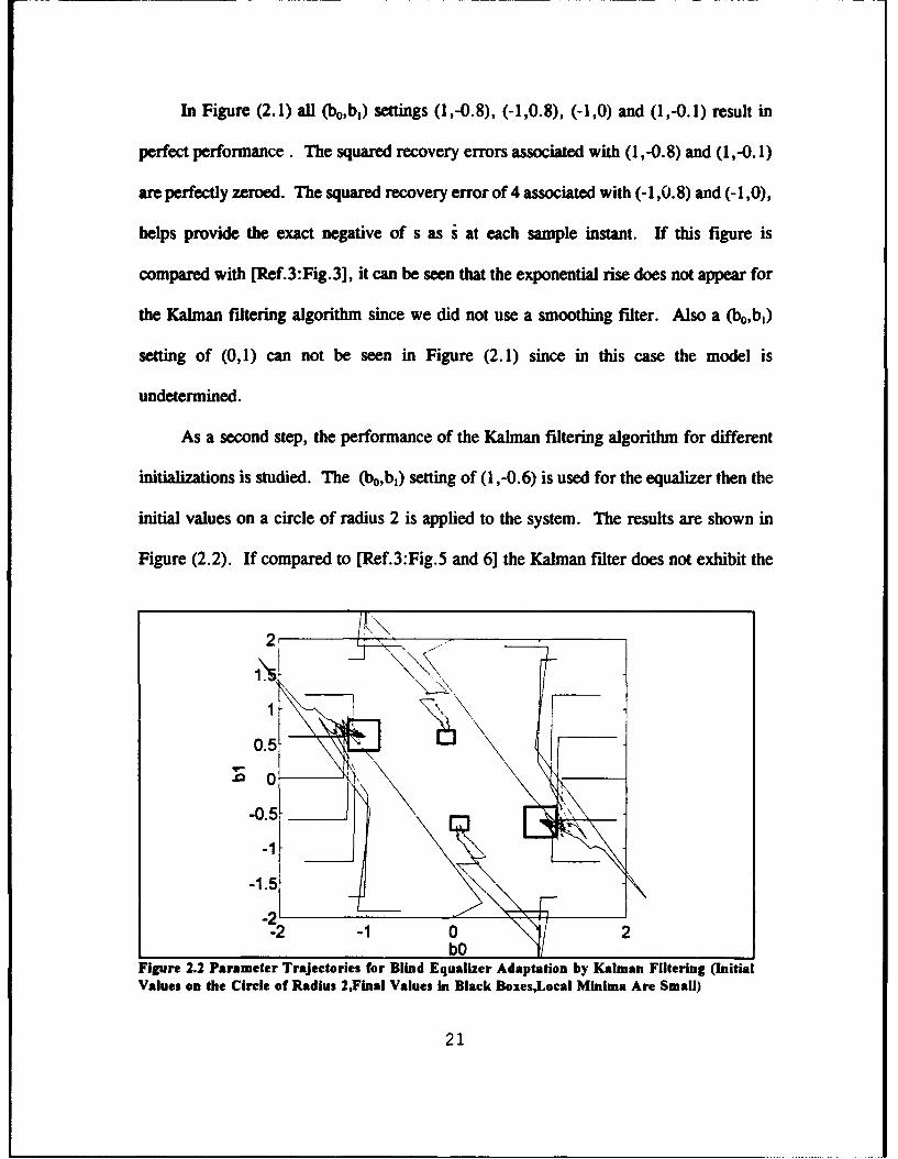
In Figure (2.1) all (bo,bl) settings (1,-0.8), (-1,0.8), (-1,0) and (1,-0.1) result in
perfect performance. The squared recovery errors associated with (1 ,-4.8) and (1,-0. 1)
are perfectly zeroed. The squared recovery error of 4 associated with (-1,0.8) and (-1,0),
helps provide the exact negative of s as i at each sample instant. If this figure is
compared with [Ref.3:Fig.3], it can be seen that the exponential rise does not appear for
the Kalman filtering algorithm since we did not use a smoothing filter. Also a (b0,bl)
setting of (0,1) can not be seen in Figure (2.1) since in this case the model is
undetermined.
As a second step, the performance of the Kalman filtering algorithm for different
initializations is studied. The (b0,b1 ) setting of (1 ,-4.6) is used for the equalizer then the
initial values on a circle of radius 2 is applied to the system. The results are shown in
Figure (2.2). If compared to [Ref.3:Fig.5 and 6] the Kalman filter does not exhibit the
2
0.5-
01-0.5
-1.5-A
"-2 -1 0 2bO
Figure 2.2 Parameter Trajectories for Blind Equalizer Adaptation by Kalman Filtering (InitialValues on the Circle of Radius 2,Final Values in Black BoxesLocal Minima Are Small)
21

amount of local minima shown by other CMA algorithms. For most of the initial
conditions the parameter vector converges to the global minima.
For a perfect solution to the problem, we need to understand the behavior of the
algorithm when convergence to local minima occurs. If we initialize (b0,bi) at (0,2) the
algorithm converges to a global minimum. The normalized squared recovery errors
between s and t for this case show a distribution equivalent to N(O,1). The situation is
shown in Figure (2.3).
0.4
mean--0.1829
0.3 var-1.492
0.2
0.1
'. Ik
-30 -20 -10 0 10
Figure 2.3 Distribuion of Squared Reoveay Errors When Algorithm Globlly Converges
Also, we can see from Figure (2.2) that there are initial conditions which lead to
local minima. As in the example of initialization (0.6,-1.9), the algorithm converges to
local minimum. In this case, the normalized squared error between s and t has a larger
mean and variance than the first case. Also, it does not show a normal situation. The
22

situation is shown in Figure (2.4). This property can be used to determine the
convergence to a local minimum.
0.4
mean=4.299
0.3 var-40.2
0.2
0 ..... ,.,ngmlF1n b i]ff-40 -30 -20 -10 0 10
Figure 2.4 Distribution of Squared Recovery Errors When Algorithm Locally Converges
The studies up to this step show that blind equalization algorithms using Kalman
filtering seem to work better than other algorithms in terms of convergence rate for
linear, time invariant, stable channel models and binary sources using BPSK. However
they still suffer from the local cc,&,vergence problem as seen for the CMA algorithms.
23

M. BLIND EQUALIZATION ALGORITHM BY USING
PARALLEL KALMAN FILTERING
As seen in the previous chapter, the algorithm based on the extended Kalman filter
for blind equalization, suffers from the local convergence problem, as most of the other
CMA algorithms. For the algorithm to be applicable, we need to address this problem.
As a candidate solution we choose a particular parallel Kalman filtering approach, which
is described in detail in [Ref.4]. In this chapter, we will present this algorithm and
discuss the results of our studies with this algorithm.
A. DEVELOPMENT OF THE PARALLEL KALMAN FILTERING
ALGORITHM
This algorithm is an approximation to the optimum maximum a posteriori (MAP)
sequence estimator for a priori unknown channels. The sequence probabilities can be
computed using the innovations derived from a bank of Kalman filters.
In the discrete-time channel and signal model, x (t) denotes the output of a
matched filter at time t, s (t) is the current transmitted symbol and (an (t) represent
the effective time varying channel coefficients. For BPSK, the s (t) are real valued,
taking on values {+ 1 ,-1}. The channel coefficients an (t) represent the convolution of
the actual intersymbol interference (ISI) channel impulse response with that of a
prewhitening filter, which is included to insure that the additive noise samples, n (t),
are uncorrelated.
24

N.
x(t)= a.(t) s(t-n)+On(t) (3.1)
The additive noise sequence is complex white Gaussian with variance or I and Nb+ 1 is
the length of the channel impulse response.
For convenience in the derivation, the following sequences are also defined for the
ith of M'+' possible sequences, where M is the symbol alphabet size:
The cumulative measurement sequence,
x,={x(t) ,X(t-1), .. x(o)}
"A cumulative data sequence,
Di,,={ di,(t), 4. (t-1),..ý. (0)}
"A data subsequence, comprising the data symbols associated with the channel
coefficient vector g (t) at time t,
Dj',ýv ={ (. ( t) k ,( t- ,. , 1) t -Nb).
In the development of the Kalman filter channel estimator, it is assumed that the
coefficient bn (t) evolve according to the following complex Gaussian
autoregressive(AR) process model
_b(t+1)=Fb(t)+w(t) , (3.2)
with the coefficient vector defined by
25
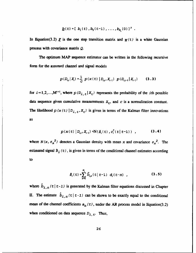
1b(t)=[ b,(t),b 2 (t-1), ... ,bN.(O)] .
In Equation(3.2) E is the one step transition matrix and _w(t) is a white Gaussian
process with covariance matrix Q.
The optimum MAP sequence estimator can be written in the following recursive
form for the assumed channel and signal models
p (Dj, I X,) =1p (x (t) ID',X-)p(j- 11) (3.3)1
for i=1,2,...,Mt ÷1 , where p (D1 , t I Xt) represents the probability of the ith possible
data sequence given cumulative measurements Xt, and c is a normalization constant.
The likelihood p (x (t) Di, t, x) is given in terms of the Kalman filter innovations
as
p ~ ~ t [ , _I,.) =N (S ; t) i,( ] t l (3 . 4 )
where N(x, a. 2 ) denotes a Gaussian density with mean x and covariance OC2. The
estimated signal :i (t), is given in terms of the conditional channel estimates according
to
N.B, ( 0 =E b-,,,,(tl t-1) A.(t-n) (3.5)R-O
where bi, n (t I t -1) is generated by the Kalman filter equations discussed in Chapter
I. The estimate bi, n (t It-I) can be shown to be exactly equal to the conditional
mean of the channel coefficients an (t), under the AR process model in Equation(3.2)
when conditioned on data sequence Di, t. Thus,
26

bj,.!ý t t-1) =E [b. (t) X ,-,,] (3.6)
From Equations (3.3) and (3.4), it is seen that the optimum MAP sequence
estimator requires a bank of W' Kalman filter channel estimators, each conditioned on
a different D1 , t. The MAP probabilities of each sequence are then obtained as a product
of the corresponding innovations likelihoods.
By using the concept of reduced state sequence estimation (RSEE), the algorithm
becomes as follows (more detailed derivation can be found in [Ref.4]):
i. Define observation vectors
hi,(t) =[I di (t) ,oA.(t-1) , . ,d, (t-Nb)]1 (3.7)
ii. Compute conditional innovations covariances
a, ( t I t- 1) =hi (t) hir (t) + a (3.8)
iii. Compute signal estimates
n.O
iv. Compute conditional measurement update
bi (t I t) 41,(t I t-1) + 2 hi (t) (x(t) -fi,(t) )(3.10)a2 (tI t-1)
27
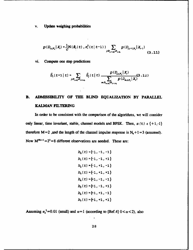
v. Update weighing probabilities
(3.11)
vi. Compute one step predictions
p(j..Nb I X')
S(tlp (D,.,,,IX,)
B. ADMISSIBILITY OF THE BLIND EQUALIZATION BY PARALLEL
KALMAN FILTERING
In order to be consistent with the comparison of the algorithms, we will consider
only linear, time invariant, stable, channel models and BPSK. Then, s(t) W {+1,-1}
therefore M=2 ,and the length of the channel impulse response is Nb+ 1 =3 (assumed).
Now M +•1 -=23- =8 different observations are needed. These are:
ho(t) ={-l, -1, -1}
h, (t) ={-i, -1, +1}
h2 (t) ={-i, +1, -1}
h3 (t) ={-0, +1, +1}
h4 (t) ={+1, -1, -1}
4 (t) ={+1, -1, +1}
h 6 (t) ={+3, +1, -1}
h7 (t) ={+l, +1, +1}
Assuming ar2=0.01 (small) and ae=1 (according to [Ref.4] O<oa<2), also
28

2,-1 exp- (x(t) -9, (t) )IN=fj(),a tIt1 x- (3.13)
Substitution of all these parameters into the algorithm discussed in Section A yields the
performance with various fixed equalizer parametrization, which is shown in Figure
(3.1).
5,
4L4..
(A)[-1,O.81 ; (B)[-1,o] ; (C)[1,-O.1] (D)[1,-4.81
0 100 200 300 400 500Iterations
Figure 3.1 Smoothed Squared-Recovery-Error Time Histories for Different Fixed EqualizerParametrizations [(be ,bj)]
In Figure (3.1) all (bo,b 1) settings result in perfect performance though H(z)*1.
Also, the phase ambiguity problem which occurs in the extended Kalman filtering
29
algorithm is solved. The exponential rise does not appear since we did not use a
smoothing filter, and (bo,b) setting (0,1) does not appear in the figure since the model
is undetermined for this case.
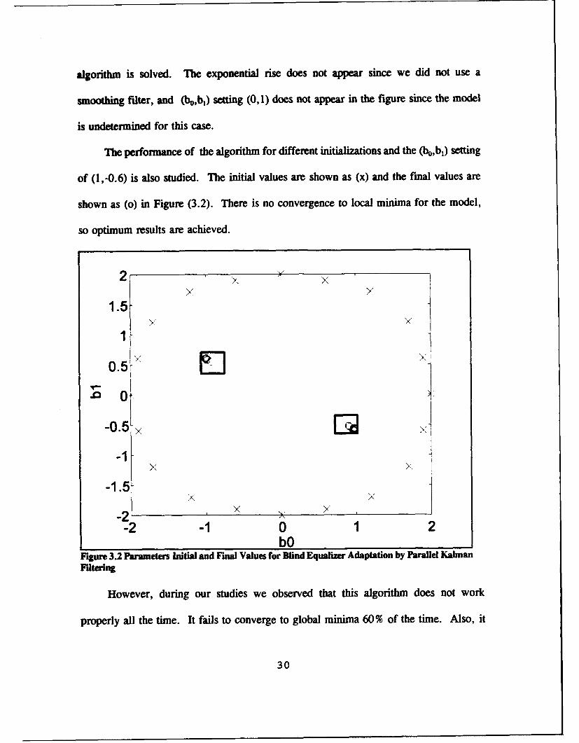
The performance of the algorithm for different initializations and the (b0 ,b,) setting
of (l,-0.6) is also studied. The initial values are shown as (x) and the final values are
shown as (o) in Figure (3.2). There is no convergence to local minima for the model,
so optimum results are achieved.
2 - x
1.5-
#-1
-0 .5 1,x
"-.5"x X-2X X 1-2 -1 0 1 2
bOFigure 3.2 Parameters Initial and Final Values for Blind Equalizer Adaptation by Parallel KalmanM',tering
However, during our studies we observed that this algorithm does not work
properly all the time. It fails to converge to global minima 60% of the time. Also, it
30

can not work as well as the extended Kalman filtering approach in nonminimum phase
systems. When the algorithm converges to local minima, there is no way to determine
the situation with this algorithm as in the Kalman filtering approach. So the algorithm
becomes unreliable, since we can not decide whether the global minima have been
reached or not by any means. The usage of multiple Kalman filters is another
disadvantage of this algorithm, when the cost is considered.
31

IV. APPLICATION OF HIDDEN MARKOV MODELS TO BLIND
EQUALIZATION ALGORITHMS WITH KALMAN FILTERING
In communication systems the transmitted sequence s (t) is not a random
independent identically distributed (i.i.d.) sequence. Indeed forward error correction
(FEC) coding is applied to a message sequence u (t), in order to produce the
transmitted sequence s (t). At this point we realized that, none of the algorithms
known so far uses the statistics of the transmitted sequence s (t), which might be useful
for the channel equalization. Obviously, if we decide to use the statistics of the
transmitted sequence s (t) in equalization, we can combine the equalizer with the FEC
decoder. It is a fact that, most of the FEC coding systems which are used in
communication systems, are convolutional coders and decoders. They mostly use the
Viterbi soft decoding technique, which is an optimum estimation for Markov models.
So in our new approach we will try to combine the Kalman filtering algorithm with
hidden Markov models.
A. HIDDEN MARKOV MODELS
Consider a system that may be described at any time as being in one of a set of N
distinct states indexed by {l,2,3,...,N}. At regularly spaced, discrete times, the system
undergoes a change of state according to a set of probabilities associated with the state.
We denote the time instants associated with state changes as t= 1,2,3,... , and we denote
32

the actual state at time t as qt. For a discrete time, first order, Markov model, the
probabilistic dependence is truncated to just the preceding state.
p[L=jcq,-=i, q. 2 =k, Q. 3=1, ... ]=pIq,=jqI,=i] (4.1)
Furthermore, those processes in which the right hand side of Equation (4.1) is
independent of time, lead to the set of state transition probabilities aij of the form
a,=p[q=j~q-1 =i] , lsi,jsN (4.2)
with the following properties
a0,0O V j,i
N (4.3)ao,=1 . V i
j-1
The notation:
7,=p [q, =i] sisN (4.4)
is used to denote the initial state probabilities.
The concept of Markov models can be extended to include the case in which the
observation is a probabilistic function of the state, so the resulting model (which is called
a hidden Markov model) is a doubly embedded stochastic process with an underlying
stochastic process that is not directly observable (it is hidden) but can be observed only
through another set of stochastic processes that produce the sequence of observations.
As a result a hidden Markov model (HMM) for discrete symbol observations can be
characterized by the following elements:
33

i). N, the number of states in the model,
ii). M, the number of distinct observation symbols per state. We denote the
individual symbols as
v= (V, .V2 V3 . .,VM)
iii). The state transition probability matrix A- (aij) where
au=p [q., =j I %=i] lsi, jsN (4.5)
iv). The observation symbol probability distribution, B= (bj (k) ), in which
bt (k) =p [ o,=v =j] (skM (4.6)
defines the symbol distribution in state j, where j=1,2,3,...,N. Also a typical
observation sequence of the model can be shown as
o= (ox, 02,0.3, .. I, OT)
v). The initial state distribution w= (?i}) in which
wi=p [ q,=i] lisiN (4.7)
So a complete specification of a HIMM requires specification of two model
parameters, N and M, specification of observation symbols, 0, and the specification of
the three sets of probability measures A, B and w. The compact notation
X= (A,B, 7r) (4.8)
"is used to indicate the complete parameter set of model. Given the appropriate values
of N, M, A, B and 7r, the HMM can be used as a generator to give an observation
sequence
34

O= (o,,0,F 023,..., oT) (4.9)
where each observation ot is one of the symbols from V, and T is the number of
observations in the sequence. This model is the main model used for FEC coding, and
it works as follows:
1. Choose an initial state %1 -i according to the initial state distribution w,
2. Set t-=i,
3. Choose ot=Vk according to the symbol probability distribution in state i, i.e.,
bj (k),
4. Transit to a new state q,+i=j according to the state transition probability
distribution for state i, i.e., aij,
5. Set t=t+1; return to step 3 if t<c, otherwise, terminate the procedure.
Now, let us approach the problem from our point of view. We have the
observation sequence 0, which is produced by the model, described above, and we know
the model X. We need to choose a corresponding state sequence q= (q1 , q2 , • ,q)
that is optimal in some sense (i.e., best explains the observations).
We can define the posteriori probability as
(i_[0, =iIX] p[O,q =iIX]P[OIX] N (4.10)
p(0XJ pE0, cj,=i I X]
Using - t (i) we can solve for the individually most likely state qt * at time t, as
35
cl" =arg min,,-'- [7Y,( W I stsT (4.11)
Using this criteria iteratively the single best state sequence (path) can be found.
To find the single best state sequence q, for the given observation sequence 0, we need
to define the quantity
(4.12),(i) =-max,, . ....,,.P [q,, q 2 , • • -, , •ki, oj , 02, .. o, OilX1
that is the best score (highest probability) along the single path, at time t, which
accounts for the first t observations and ends in state i. By induction we can compute
it recursively as
6,(i)= may. 6,-(j) p[qf=i k.=j] p[o, Iq=i] (4.13)
To actually retrieve the state sequence, we need to keep track of the argument that
maximized Equation (4.13), for each t and j. The formal technique for doing the job
is based on dynamic programming methods, and is called the Viterbi algorithm. [Ref.5]
B. COMBINING KALMAN FILTERING ALGORITHMS WITH 1MM
In general, a message sequence u (t) is coded by a HMM. The block diagram
of an overall communication scheme is shown in Figure (4.1). The discrete coder states
z (t) where z (t) eZ= (1, 2, 3, ... , L and the output sequence s (t) are dependent
on the older coder states and the input sequence u (t) to the coder. Thus,
z(t+1) = F[z(t),u(t) (4.14)
s(t)= G[z(t),u(t)]
36

sorecoder -a channel -iequalizer -*decoder
Figure 4.1 Block Diagram of the Communication System
As we stated in Chapter II before; the vector Xt represents the received signal values
and the vector Wt represents the state coefficients of the equalizer. So we can show the
output of the equalizer as
y(t) =( t)= WT(t) X,(t)+ e(t) (4.15)
where e (t) is estimation error described in Chapter I.
In extended Kalman filtering approach we assumed the channel changes slowly and
the model is defined in Equation (2.21). We account for drifts in channel parameters by
the recursion
37

W, (t+1) ,W, (t) +v(t) (4.16)
Then combining the Equations (4.14), (4.15), and (4.16) we can represent the overall
model of equalizer and decoder as
z (t+1) = F[z (t) , u(t) I
w,(t+l) =w, (t) +v(t) (4.17)
0= G[z(t),u(t)]- W,(t) X,(t)+ e(t)
The difficulty with this state space model is that the state [Z (t), _W(t) J is a
mixture of a discrete component Z (t) and a continuous one ff(t).
The estimation algorithm is based on the fact that, given the sequences
7-t(t) = [z(1),z(2),... ,z(t)]
Y,(t) =[y(1),y(2),...,y(t)]
the estimate of w
E= [ W, Z, , T 1(4.18)
is well defined, and recursively computable by standard Kalman filtering techniques.
An overall recursion along the same lines as the estimation for hidden Markov
models can be devised for this case.
The suboptimal optimization is based on the definition
6,(i) =maxj p(2/(t-1) ,z(t) =i, Y,(t)) (4.19)
where ztJ (t-1) is the optimum path up to state z (t-1) =j. By induction we can
update 6 t (i) as
38
-,(i .-.a, [p (y (t) t -1)(t-l),( t) =i, Y, ( t-1))p (z(t)=i z (t -1)=j) 6,_,(j)]
(4.20)
and keep track of the indices on the optimal path
J -arg max [p (y(t) 12,ý_ (t-1) , z(t) =i, Y, (t-1) )p(z (t) =i z (t-1) =j) 6,.(j) ]
(4.21)
The optimal path up to state z(t)=i is then updated as
A/(t)=2/-,(t-1) U z(t)=i (4.22)
Also we know all the possible previous states j and the state coefficient estimates of the
channel up to this state w,.1q) is already computed by Kalman filtering as stated in
Equation (4.18). So we can determine the optimum estimates of the channel state
coefficients by the following procedure:
@,ij) =0,-,(j) + jc,_,[G [j, u(t)] _(j X, (t) + e (t) (4.23)
W, (i) =most likelyj , (i Ij)
C. FEASIBILITY OF HMM AND KALMAN FILTERING APPROACH TO
BLIND EQUALIZATION
This new algorithm works almost perfect in linear, time invariant, stable, channel
models and BPSK. This new algorithm seems to be more capable than the previous
ones, and we applied it to more complex channels. We have used different feasible FEC
encoders (with different rates and constraint lengths), BPSK signaling, additive white
39

Gaussian noise (AWGN) and different signal to noise ratios (SNR) in the studies. The
results are presented in Figures (4.2) through (4.4).
Since the perfect equalization requires
a(t) * b(t) = I
the complete impulse response of the combination of the channel and the equalizer must
appear as an impulse function, which is the case in our studies (shown at the left upper
corner of the figures).
By looking at the results, this new algorithm recovers the sent message without
errors after a couple of iterations, which are very small compared to the length of the
transmitted sequence. This algorithm works much better in high SNR values. Errors
do occur if SNR drops under 5 dB. but further studies are needed to determine the exact
margin. With this kind of performance, this algorithm can also be a candidate to address
the channel drifting problem.
40

VIWe Msp d -l+" ss6rdmw ssage
0.0
0.1 -0 10 20 30 40 0 20 40 so
0.
0 20 40 0 0 20 40 s0
Figure 4.2 Channel and Message Estimation for Rate=I/2,Con.Len=3 Encoder with High SNR
41

bpqub sp odtq ,med mAessag
0.6-
0 10 20 30 40 0 10 20 30 40
am message _ _ _
0.
IfI
0 10 20 30 40 0 10 20 30 40
Figure 4.3 Channel and Message Estimation for Rate=1/3, Con.Len=3 Encoder with High SNR
42

knpks mop q salmasd messageU LiU0..AJ!\"
440 10 20 30 40 0 20 40 s0
swmesage _ _ _
-0.
0 20 40 60 0 20 40 60
Figure 4.4 Channel and Message Estintation for Rate= 1/2,Con.Len=7 Encoder with High SNR
43

V. SIMULATION AND RESULTS
We have simulated a flat Rayleigh fading channel and tried our new algorithm on
it, in order to see its feasibility in overall communication systems. The block diagram
of our simulation scheme is shown in Figure (5. 1).
I CHANNEL
PAOIMG
Figure 5.1 Block Diga of the Simlation Scheme i•t DBISK and Flat Rayleigh Fading
In the simulation DBPSK is used as a modulation scheme. DBPSK has hardware
simplicity and does not require phase coherency. It is popular for channels where the
phase shift changes slowly compared to the bit duration.
44
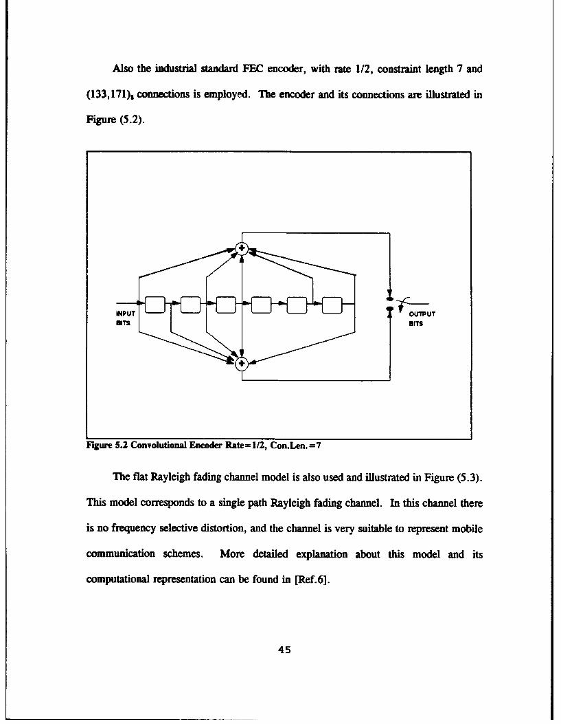
Also the industrial standard FEC encoder, with rate 1/2, constraint length 7 and
(133,171)s connections is employed. The encoder and its connections are illustrated in
Figure (5.2).
BTS BITS
Figure 5.2 Convolutional Encoder Rate= 1/2, Con.Len. =7
The flat Rayleigh fading channel model is also used and illustrated in Figure (5.3).
This model corresponds to a single path Rayleigh fading channel. In this channel there
is no frequency selective distortion, and the channel is very suitable to represent mobile
communication schemes. More detailed explanation about this model and its
computational representation can be found in [Ref.6].
45

AVON GENERATOR
RtC FILTER
SRC FF LTER
I CHA. (
0 CHAN. (?
RC F FLTRI
AV•GN GENERATOR
Figure S.3 Block Diagram of Flat Rayleigh Fading Channel Model
The results of the simulation using a signal to noise ratio (SNR) of 13 dB. is given
in Figure (5.4). As it can be seen from the results of our simulation, the combination
of equalizer and decoder by HMM and Kalman filtering approach performs fairly good
in complex channels and under channel fading conditions.
46

0 5 10 15 20 25 30 35 40 45 50
0 5 10 15 20 25 30 35 40 45 50
.1.
"-1 -0 . 10 15 20 25 30 35 40 46 so
Figure 5.4 Estimation of the Message Sequence in Flat Rayleigh Fading Channel Using DBPSKand Rate= 1/2 FEC Code
47

VI. CONCLUSIONS
An alternative algorithm for blind equalization of digital communication channels,
is derived and studied by using extended Kalman filtering and hidden Markov models.
This new algorithm seems more efficient since it takes the statistics of the transmitted
sequence into consideration. It seems to be more robust with respect to local minima,
and channel drifting problems.
Hardware implementation of this algorithm might be cost effective since it
combines two major components of a receiver, namely the equalizer and the decoder into
a single component.
Future studies can determine the overall performance of this algorithm under
different channel conditions and for different communication schemes.
48

APPENDIX A. MATLAB SOURCE CODES
The algorithms described in Chapters II,m and IV were implemented using
MATLAB software and are listed below.
A. BLIND EQUALIZER FOR LINEAR, TIME-INVARIANT, STABLE
CHANNELS BY USING EXTENDED KAIMvIAN FILTER
% Filename: eqkalm.m% Title : Blind equalizer for linear,time-invariant,stable channels by using Kalman filtering% algorithm% Date of last revision : 15 Jul 1993% Comments : This program produces an array of random digital signal values,% (either + or -1) to represent the message signal.The length of message signal% depends on the sampling amount m(of course bigger m makes better% estimation). Then this signal is applied to a channel such as:[x(t) x(t-l) ...% x(t-n)] where the coefficiants defined by user.To estimate the equalizer% coefficiants, a rectangular window over the received signal values, is going to% be used such as[x(t) x(t-1) ... x(t-n)] where (n+ 1) represents the # of values% taken into account by the window (and by the equalizer).In this way program% tries to predict real coefficients of channel.If values match equalizer design% will be perfect.% Averaged squared recovery error due to the channel and qualizer,performance% due to the different initializations and normalized squared error distributions% can be plotted.% Input variables :% f : The coefficients of the channel as a vector% i m: Sampling amount% wt: Initial values of the coefficients at the equalizer as a column vector% sel: Selection to continue with the calculation% op: Options to plot different schemes% Output variables :% b : The estimated values of the channel coefficients by equalizer% Associated functions : None
clear;f=input('NOW ENTER the coefficients of your channel as vector.:');m=input(' ENTER the value of m (sampling amount) ..................sel=input(' ENTER I to continue .................
49

S S% Produce inmage % %%nwlength(f)-1;y-sin(randn(1 ,(m+ n)));
while sel - -1wt-'.Ol1%nes((n+ 1),(m+n));wt(:,n)-input('ENTER the initial coefficiants for your equalizer as column vector..:');
% % % Arrangements % % %xt-zeros((n+ 1),l);et-zeros(1 ,m);errt-zeros(1 ,m);ay-eye((n+ 1),(n+ 1));pt-diag([le- , le-li);x -zeros(l,(n + 1));
% %% Pass message through the channel %% %for i=n+I:m+n
x(i)=(-f(2:n+ 1).*x(i-1:-1:i-n)+y(i))/f(1);end
% %% Kalman filtering % %%for j =n+ l:m+ n
xt=(xoj:-l :j-n))';wtl may~wt(: i-i);
ptl =ay~lpt~ay';gt-ptl *c'*inv(c~pt1 *c' +.01);
et(:,j-n)= I-ytl;errt(: j-n)=et(: j-n)Isqrt(c*pt*c' +.01);
end%%% Results %%%b=wt(:,m+n)'pause
% % % Estimation errors % % %for k=n+lI:n+m
r(k)=(b(1 :n+ I)*x(k:-1 :k-n)');s(k) = (0)-r(k))^2;
end%%% Plots %%%
disp('For the graphs you have the following options:');disp('ENTER I to see aver. squ. error due to the chan. & equa.');disp('ENTER 2 to see performance due to the different initial izations');disp('ENTER 3 to see normalized squared error distributions');op =input('ENTER 0 to quit .......while op = =1,
plot(s(n+ 1: n +m))
50
grid;xlabel('Iterations');ylabel('(u(k)-u(k)) );pausedisp('For the graphs you have the following options:');disp('ENTER 2 to see performance due to the different initializations');disp('ENTER 3 to see normalized squared error distributions');op-input('ENTER 0 to quit .........
endwhile op= -2,
axis([-2 2 -2 2j);plot(wt(l ,:),wt(2,:))
grid;xlabel('bO');ylabel('bl ');pausedisp('For the graphs you have the following options:');disp('ENTER 1 to see aver. squ. error due to the chan. & equa.');disp('ENTER 3 to see normalized squared error distributions');op=input('ENTER 0 to quit .........
endwhile op= -3,
[n2,x2] =hist(errt,30);k2=-4:.01:4;gt= l/sqrt(2*pi)*exp((-(k2."2))/2);m2=max(gt);[xb2,yb2] = bar(x2,((n2/max(n2))*m2));plot(k2,gt,xb2,yb2);ort=mean(errt);var= (std(errt)A2);gtext(['mean = ',num2str(ort)]);gtext(['var=',num2str(var)]);pausedisp('For the graphs you have the following options:');disp('ENTER 1 to see aver. squ. error due to the chan. & equa.');disp('ENTER 2 to see performance due to the different initializations');op=input('ENTER 0 to quit .........
end
disp(' ENTER 0 to exit to matlab .................
sel= input(' ENTER 1 to continue .................
end
end;
51

B. BLIND EQUALIZER FOR LINEAR, TIME-INVARIANT, STABLE CHANNELS BY
USING PARALLEL KALMAN FILTERS
S Filename : parkal.mS Title Blind equalizer for linear,time-invariant,stable channels% by using parallel Kalman filtering algorithmS Date of last revision : 18 Jul 1993% Comments : This program produces an array of random digital% signal values, (either + or -1) to represent the message% signal.The length of message signal depends on the sampling
Sam ount m (of course bigger m m akes better estim ation).Then% this signal is applied to a channel such as:[x(t) x(t-1) ...% x(t-n)I where the coefficiants defined by user.To estimate% the equalizer coefficiants, a rectangular window over the% received signal values, is going to be used such as[x(t)% x(t-1) ... x(t-n)] where (n+ 1) represents the # of values% taken into account by the window (and by the equalizer).% Also each symbol in the message alphabet is assigned to% a specific Kalman filter.In this way program tries to% predict real coefficients of the channel.At the end correct% channel parameter estimations appear at least at one of the% Kalman filters in the bank.If values match equalizer design% will be perfect.( Program works for alphabet size 4 only)% Averaged squared recovery error due to the channel and% equalizer,performance due to the different initializations% and normalized squared error distributions can be plotted.% Input variables :% f : The coefficients of the channel as a vector% m : Sampling amount% bi: Initial values of the coefficients at the equalizer as% a column vector% sel: Selection to continue with the calculation% sec: Options to plot different schemes for different filters% Output variables :% b* : The estimated values of the channel coefficients by% associated Kalman filter *.
% Associated functions : None
clc;
clear;f=input('NOW ENTER the coefficients for the channel as vector(2 elements).:');m-=input(' ENTER the value of m (sampling amount) ..................sel=input(' ENTER 1 to continue .................hold off
52

while seI-- Ibi-inputCENTER the initial coelficiants for your equalizer as column vectr..:');n-length(O)-I;y -sign(randn(1 ,(m +n)));r-zeros(1,(n+ 1));zO-ones(l,(n+ 1));zI -ones(l,(n+ 1));z2=ones(l,(n + 1));z3 -ones(1,(n + 1));et-zeros(I ,m);errt-zeros(1 ,m);for i-n+l:m+nr(i)=(f(1:n+1Yyi-in);
% r(i)=(-f(2:n+ 1).*r(i-1 :-1 :i-n)' +y(i))If(1); % Nonrecursive caseend
bO=bi;%hO=[-1 -1];%sigo=bO*hO' +.01; % FOR EACH FILTERp0-0.25;%
bl =bi;hl=[-1 ]sigi =h1*hl'+ .01;p1 =0.25;
b2=bi;h2=[1 -11;sig2=h2*h2' +.01;p2 =0.25;
b3=bi;h3=[1 1];sig3=h3*h3'+.01;p3=0.25;
for j=n+ 1:m+npOO-pO; %FOR EACH FILTERp I =pi;p2 2 -p2;p33=p3;
sO=sum(bO.Th0');%bO=bO+ ((1/sigO)Th0'*(roj)-sO));%NO= II(sqrt(2*ipi*sig0))*exp((-(rGj)-s0).A2)I2*sig0); % FOR EACH FILTERpO=NO*(p00+pl 1);%
53

&1-sum(bI."hi');hi -h I(1sg~l'rj-l)N I- 1I(sqrt(2spi~sig1))*exp((-(roj)-s ).A2)/2*sig 1);p1I - N1I p22 +p33);
s2-sum~b2.*h2');b2 -b2+ ((Ilsig2)h2'*(roj)-s2));
p2-N2*(pO+pi 1);
£3 -sum(b3 .'h3');W3 -bW + ((Il/sig3) *h3'*Nro)-s3));N3 - 1/(sqrt(2*Ipi~sig3))*exp((-(raj)-s3).A2)/2*sig3);p3=N3*(p22 +p3 3);
pn-pO+pI +p2+p3; %NORMALIZERpO-pO/pn; %FOR EACH FILTERp1 =pl/pn;p2=p2/pn;p3 =p3/pn;
bO-bO*(pO/(pO+pl))+bI*(pl/(pO+pl)); %FOR EACH FILTERb I = b2*(p2/(p2 +p3)) +bW*(~p3/(,2 + p3));b2=bO;b3=bl;
end
bO' % FOR EACH FILTERbi'b2'b3'
for k=n+1I:m+n% zO(k)=(bO(1:n+ 1)'*r(k:-1:k-n)'); % NONRECURSIVE CASE% zl(k)=(bl(1 :n+ 1)'*r(k:-1 :k-n)'); %
zO(k) =(zO(k-I :-1 :k-n)*(-bO(2:n +1)) +r(k))/bO(1);
sOM)=(l-(zO(k)A2)); %A2;seO(k) = s(k)Isqrt(sigO);
sel (k) = si(k)Isqrt(sig 1);end
sec=input(' ENTER 1 for 1&3;2 for 2&4 channels.........
54

while sec -- IS plot(bO(l,:),bO(2,:),'wo'); %% plot(bi(l,:),bi(2,:),'wx') %% axis([-2 2 -2 21);%% bold on % TRAJECTORIES% grid;%% xlabcl('bO');%% ylabei('bl');%% pause%
% plot(slI(n +l:n +m),'w') %% axis([0 500 -l5]); %% grid; % RECOVERY ERRORS% xlabel('lterations'); %% ylabel('(u(k)-u(k)) %)% pause %[n2,x2J =hist(se0,30); %k2=-4:.01:4; %gt= I/sqrt(2*Ipi)*exp((-(k2.^2))I2); %m2-max(gt); %[xb2,yb2J =bar(x2,((n2/max(n2))*m2)); % HISTOGRAMSplot(k2,gt,'w-',xb2,yb2,'w'); %ort-mean(se0); %
gtext(['mean =',num2str(ort)]); %gtext(['var =',num2str(var)]); %pause %
sec=input(' ENTER 1 for 180;2 for 2&4 channels.........end
while sec =2 % different parts are as shown above% plot(blI (1, :),b I1(2, :),'wo');% plot(bi(1 ,:),bi(2,:),'wx')% axis([-2 2 -2 2]);% hold on% grid;% xlabel('bO');% ylabel('bl');% pause
% plot(s I(n +1:n +m),'w')% axis([0 500 -1 5]);% grid;% xlabel('Iterations');% ylabel('(u(k)-u(k))')% pause[n2A2=hist(sel ,30);k2=-4:.01 :4;gt= I Isqrt(2*pi)*exp((-(k2.A2))/2);
55

m2-max(gt);[xb2,yb2 =-bar(x2,((nm2x(n2))*m2));plot(k2,V,'w-',xb2,yb2,'w');ort-mean(sel);var=(std(sel)A2);gtext(['mean- ',num2str(ort)]);gtext(rvar- 'num2str(var)); %pause
sec-input(' ENTER I for 1&3;2 for 2&4 channels ................. :)
end
hold onsel-input( ENTER I to continue ................. :9);
end
end;
C. BLIND EQUALIZER FOR LINEAR, TIME-INVARIANT, STABLE CHANNELS
BY USING KALMAN FILTER AND 11MM ALGORITHM
% Filename: trynew.m% Title Blind equalizer for linear,time-invariant,stable channels% by using Kalman filtering and HMM algorithm% Date of last revision : 25 Aug 1993% Comments : This program produces an array of random digital NRZ, BPSK% signal values, (either + or -1) to represent the message% signal.The length of message signal depends on the sampling% amount m(of course bigger m makes better estimation).Also% applies a FEC code by HMM rate choosen by the user.Then% this signal is applied to a channel such as:[x(t) x(t-1) ...% x(t-n)] where the coefficiants defined by user.To estimate% the equalizer coefficiants, by Kalman filtering and HMM% approach.Overall impulse response of the system, sent and% recived sequences are plotted as well as the errors due to% the equalizer% Input variables :% m : Length of the message% Output variables :None% Associated functions : bpskgen.m% conenc.m% awgn.m% eqcondec.m
m•=input('ENTER THE LENGTH OF MESSAGE YOU WANT:');mes-=bpskgen(m);
56

sig -conenc(mes);an -zeros(sizs(sig));num - [1,0.6,0.4,0.31; den =zeros(size(num)); den(1) =1;% num-[1,O]; den=[l,-0.6];xt-filter(num,den,sig); % channel%xn-xt; % no noisexn-awgn(xt,0.277); % 13 dB SNR%xn-awgn(xt,0.447); % 5 dB SNR%xn-awgn(xt,0.577); % 3 dB SNR%xn-awgn(xt, 1); % 0 dB SNRh =dimpulse(num,den,20);[info,tmax] =eqcondec(xn,h);pausesubplot(223),plot(mes(l :tmax),'w'), title('actual message')subplot(224),plot(mes(l :tmax)-info(l :tmnax),'w'), tide('errors')end % of program
function Y - awgn(Xsigma)% AWGN GENERATOR% 07-31-1993% Awgn is an m-file that adds awgn noise to the matrix X% Where sigma is standart deviation of the noise% Ec/No- 1I/(2*sigmaA2).[rr,ccJ =size(X);
W =randn(rr,cc)+ i*randn(rr,cc);Y=X+sigma.*W;disp('AWGN IS ADDED TO SIGNAL');
function u =bpskgen(k)% BPSK GENERATOR% 08-01-1993% This m-file accepts k the number of bits that will be returned% in the vector u which is a BPSK sequence of I+ 1,-i)u =sign(randn(size(l :k)));disp('A random message is generated and coded in bipolar NRZ form');
function s=conenc(u)% CONVOLUTIONAL ENCODER% 07-31-1993% This m-file is a feedforward convolutional encoder for state transition% matrix F,output sequence matrix G and input message matrix u. The number% of convolution schemes can be increased by adding F & G matrices for new% rates.
57
disp('To use rate- 1/2 convolutional encoder ENTER I');disp('To use rate- 1/3 convolutional encoder ENTER 2');disp('ro quit encoding ENTER 0');sel -input("')while sel = - 1,
F-[1,2;3,4;1,2;3,4];
G=[0,-II,-1, 1,1,-i, 1,-i;
xffl;
s =zeros(size(G(:, 1)'));for t= 1 :length(u)
x=F(round(x),round(l.5+u(t)/2));if x==1,
sf=G(:,(round(x) + round(1.5 +u(t)/2)));elseif x= =2,
sf=G(:,(round(x) + 1+ round(1.5 + u(t)/2)));elseif x-= = 3,
sf= G(: ,(round(x) + 2 + round (1.5 + u(t)/2)));elseif x= =4,
sf= G(: ,(round(x) + 3 + round(1.5 + u(t)/2)));end % for if statements = [s,sf'];
end % for for loopdisp('Message is encoded');disp('To quit encoding ENTER 0');sel = input(")end % for while loopwhile sel = =2,
F=[1,5;1,5;2,6;2,6;3,7;3,7;4,8;4,81;
o,-1,1,-I,-1, 1,-i, 1,-I, 1, 1,-i, 1;0,-I,1,-1, 1,-i, 1,-i, 1,-I, 1,-i, 1];
x=1;s =zeros(size(G(:, 1)'));for t= :length(u)
58

x - F(round(x),round(l.5 + u(t)/2));if x--112,
sf- G(:,(round(x) + round(l.5 + u(t)/2)));elseif x==314,
sf=G(:,(round(x) + 1+ round(1.5 + u(t)/2)));elseif x- - 516,
sf-G(:,(round(x) + 2 + round(1.5 + u(t)/2)));elseif x- =718,
sf- G(: ,(round(x) + 3 + round(l.5 + u(t)/2)));end % for if statements=[s,sf];
end % for for loopdisp('Message is encoded');disp('To quit encoding ENTER 0');sel = input(")end % for while loop
function [uh,tmax] =eqcondec(x,h)% EQUALIZER AND CONVOLUTIONAL DECODER% 07-30-1993% This m-file is a channel equalizer and convolutional decoder for state% transition matrix F,output sequence matrix G ,channel parameter matrix% x and input signal s.% Simply uses the Kalman filtering algorithm with Hidden Markov Models.% The number of convolution schemes can be increased by adding F & G matrices% for new ratesdisp('To use rate= 1/2 convolutional decoder ENTER 1');disp('To use rate= 1/3 convolutional decoder ENTER 2');sel = input(")if sel = = I,
F=[1,2;3,4;1,2;3,4];
end % for if statementif sel = =2,
F--[I,5;
1,5;2,6;2,6;3,7;3,7;4,8;4,8];
59
end % for if statement
nf-lengtli(G(: .1));ns-Iength(F(:,l));n-iS5; % order of the filterth -zeros(n,ns);th(1 ,:)-5.O*ones(1 ,ns);e2-zeros(ns, 1);
P-=I *eye(n);tmin-round(nlnf)+ 1;tmax-floor(100/nf)-l;point =zeros(tmax + 1 ,ns);uhat=zeros(tma+ 1,ns);for tk-tmin:tmax,
phi =toeplitz(x(tk*nf+ 1 :tk*nf+ nf),x(tk*nf+ 1:-i :tk*nf-n +2))';facti =P*phi;fact2 -fact' V*phi;fact= inv(eye~ength(fact2)) + fact2);K -factlI fact;en2 =inf*ones(ns, 1); % start error for new layer at infinityif ns= =4,
for j =1: ns % statesfor i= 1:2 % inputsm=F~ji);if M==I,%
v=G(:,(m+i))-phi""th(:j);%elseif m= =2,%I
v =G(:, (m +1I+i))-phi'N*th(:,j); % RATE 1/2elseif m = = 3,%
v=G(:,(m+2+i))-phi'*th(:,j);%elseif m ==4,%
end%etexnp=e2(j)+v'*fact*v;if etemp < en2(m),
en2(m) = etemp;thn(: ,m)=th(: j) + Kv;point(tk + I,m) =j;uhat(tk + 1,m) =i;
end % for if statementend % for loop of i
end % for loop of jend % for while loop
60

if ns--8,for j -1:ns % states
for i=-1: 2 % inputsmumFoji);if m= -112,%
elseif m = = 314,%v-G(:,(n+ 1 +i))-phi'*th(:,j);%
elseif m = = 516, % RATE 1/3
elseifm = =718,%v=G(:,(m+3+i))-phi'*th(:,j);%
end%etemp=e20j)+ v'*fact*v;
if etemp < en2(m),en2(m) =etemp;
puint(tk + 1,m) =j;uhat(tk+ 1,m)=i;
end % for if statementend % for loop of
end % for loop of jend % for while looptb-thn;e2 = en2;P =P-fact I fact~fact I';
end[em,m] = min(e2);thf=th(: ,m);% estimated messagewhile m - = 0,
uh(tk)=2*uhat(tk+ 1 ,m)-3;m-point(tk+ I,m);tk-tk-1;
enddisp('Signal is decoded, now look to the graphs');pause
clg;hold offc -conv(h,thf);subplot(22 1), plot(c, 'ow '),title('impulse resp of ch +eq')%nu =min([length(u), length(uh)]);subplot(222),plot(uh(1 :tmax), 'w'), title('estimated message')end % of program
61
D. SIMULATION OF THE HMM AND KALMAN FILTERING ALGORITHM IN
FLAT RAYLEIGH FADING CHANNEL
% Filename: simul.m% Title Simulation of combined equalizer and FEC decoder (1MM and% Kalman filtering algorithm) in flat Rayleigh fading channel% Date of last revision : 15 Sep 1993% Comments : This program simulates the combined equalizer and FEC decoder% (HMM and Kalman filtering algorithm) in flat Rayleigh fading% channel. Works similar to previuos programs, uses DBPSK% instead of BPSK.Industrial standart, code rate 1/2 & constraint% length 7 FEC encoder is employed% Input variables :% m : Length of the message sequence% Output variables :None% Associated functions : awgn.m% bpskgen.m% conenc64.m% difecod.m% pskmod.m% fade.m% pskdmod.m% eqcod64.m
m=input('ENTER THE LENGTH OF MESSAGE YOU WANT:');mes=bpskgen(m);cme=conenc64(mes,F64,G64);len =length(cme);dcm =difecod(cme);sig =pskmod(dcm,7);sigI =sig';sig2=sigl(:);sig3 =exp(i*pi/4)*sig2;disp('POWER IS SPLITIED TO I & Q CHANNELS');I=fade(0.01,Qen+ 1)*7);Q=fade(0.01,(ien+ 1)*7);sig4=I.*real(sig3) +j*(Q.*imag(sig3));disp('Rayleigh fading is applied to signal');sig5 = awgn(sig4,0.277);[cmm,a] =pskdmod(sig,7,len);[info,tmax] =eqcod64(cmm,F64,G64);pausesubplot(21 l),plot(mes(l :tmax),'w'), title('actual message')subplot(212),plot(info(1 :tmax),'w'),title('received message')pauseprint -dmeta;
62

CIS;subplot(21 1),plot(mes(1 :tmax)-info(1 :tmax),'w'), title('errors')end % of program
function s-conenc64(u,F64,G64)% CONVOLUTIONAL ENCODER% 08-30-1993
% This rn-file is a feedforward industrial standart convolutional encoder% for state transition matrix F64,output sequence matrix G64 and input% message matrix u. F64 & G64 matrices are given as a file named incod64.mat% Be sure to load that file before working with this functionX- 1;s =zeros(size(G64(:, 1)'));for t =1:ength(u)
x =F64(round(x),round(1 .5 +u(t)/2));if X= = 119,
sf=G64(: ,(0+ round(1 .5 +u(t)/2)));elseif x == 2110,
sf-G64(:,(2+ round(1 .5+u(t)/2)));elseif x= =31 11,
sf- G64(: ,(4 + round(I .5 + u(t)/2)));elseifx = =41 12,
sf= G64(: ,(6 +round(1 .5 +u(t)12)));elseif x ==51 13,
sf= G64(: ,(8 + round(1 .5 + u(t)12)));elseif x = =61 14,
sf=G64(:,(10+round(1 .5+u(t)/2)));elseif x = = 7115,
sf= G64(: ,(1 2 + round(1 .5 + u(t)/2)));elseif x = = 8116,
sf =G64(:,(14 +round(1 .5 +u(t)12))),elseif x = = 17125,
sf= G64(: ,(16 + round(1 .5 + u(t)/2)));elseif x == 18126,
sf= G64(: ,(1 8 + round(1 .5 + u(t)12)));elseif x = = 19127,
sf=064(: ,(20 +round(1 .5 +u(t)/2)));elseif x ==20128,
sf=G64(:,(22+ round(1 .5 +u(t)/2)));elseifx = =21 129,
sf= G64(:,(24 + round(1 .5 + u(t)/2)));elseif x = = 22130,
sf= G64(: ,(26 + round(I .5 + u(t)12)));elseif x = = 2313 1,
sf= G64(: ,(28 + round( 1.5 + u~t)I2)));elseif x = =24,132,
63

sf-G64(:,(30+ round(1.5 + u(t)/2)));elseif x--33 41,
sf= G64(: ,(32 + round(1.5 + u(t)/2)));elseif x - - 34142,
sf=0G64(:,(34+round(I.5 +u(t)/2)));elseif x= =35 143,
sf-G64(:,(36 + round(l.5 + u(t)/2)));elseif x-= 36144,
sf= G64(:,(38 + round(l.5 + u(t)/2)));elseif x= =37145,sf=G64(:,(40 + round(l.5 + u(t)/2)));
elseif x==38 146,sf=G64(:,(42+ round(l.5 +u(t)/2)));
elseif x= =39 147,sf=G64(: ,(44 + round(1.5 + u(t)/2)));
elseif x= =40148,sf= G64(:,(46 + round(1.5 + u(t)/2)));
elseif x= =49157,sf= G64(: ,(48 + round(1.5 + u(t)/2)));
elseif x= =50158,sf= G64(:,(50 + round(1 .5 + u(t)/2)));
elseif x= =51159,sf= G64(: ,(52 + round(l.5 + u(t)/2)));
elseif x= =52160,sf=G64(:,(54+round(1.5 +u(t)/2)));
elseif x= =53161,sf= G64(: ,(56 + round(1.5 + u(t)/2)));
elseif x = =54162,sf= G64(:,(58 + round(1.5 + u(t)/2)));
elseif x= =55163,sf= G64(: ,(60+ round(l.5 + u(t)/2)));
elseif x= =56164,sf= G64(: ,(62 + round(1.5 + u(t)/2)));
end % for if statements=[s,sf'];
end % for for loopdisp('FEC is applied to Message(ENCODED)');
function [uh,tmax] =eqcod64(x,F64,G64)%6 EQUALIZER AND CONVOLUTIONAL DECODER% 08-21-1993% This m-file is a channel equalizer and convolutional decoder for state% transition matrix F64,output sequence matrix G64,channel parameter matrix% x and input signal s.% Industrial standart Rate 1/2 code with constraint length 7 is used F64 &% G64 matrices are defined in incod64.mat. Be sure it is loaded.
64

% Simply uses the Kalman filtering algorithm with Hidden Markov Models.% The number of convolution schemes can be increased by adding F & G matrices% for new ratesnf=lengtb(G64(:, I));ns - length(F64(:, 1));n=15; % order of the filterth -zeros(n,ns);th(l,:)-5.0*ones(l,ns);e2 -zeros(ns, 1);P- I'eye(n);tmin-round(n/nf)+ 1;tmax-floor(100/nO-1;point =zeros(tmax+ l,ns);uhat-zeros(tmax + l,ns);for tk=tmin:tmax,
phi =toeplitz(x(tk*nf+ I :tk*nf+ nf),x(tk*nf+ 1:-I :tk*nf-n + 2))';factl -P*phi;fact2 =factI '*phi;fact = inv(eyeoength(fact2)) + fact2);K = fact I *fact;en2=inf*ones(ns,l); % start error for new layer at infinityfor j - 1:ns % states
for i=1:2 % inputsm=F64(j,i);ifm==119,
v =G64(:,(0+ i))-phi'*th(:,j);
elseif m= =21 10,v = G64(:,(2 + i))-phi'*th(:,j);elseif m= =31 11,
v = G64(:,(4+ i))-phi'*th(:,j);elseif m= =41 12,
v = G64(:,(6 + i))-phi'*th(: j);elseif mn= = 5113,
v = G64(:,(8 + i))-phi'*th (:,j);
elseif m==6114,v-- G64(:, (10 +i))-phi'*th (:,j);
elseif m= =71 15,v = G64(:,(12 + i))-phi'*th(:,j);
elseif m= =8I 16,v =G-64(:,(14 + i))-phi'*th(,;
elseif m = = 17125,v = G64(:,(16 + i))-phi'*th(:,j);
elseif m= = 18126,v =G64(:,(18 + i))-phi'*th(:j);elseif m= = 19127,
v = G64(:,(20 + i))-phi'*th (:,j);
elseif m= =20128,
65

v -G64(:,(22 + i))-phi'%t(: j);elseif m - m-21129,
v -G64(:,(24+ i))-phi'*th(: j);elseif m -- 22130,
elseif m ==-2313 1,
eiseif m - - 24132,v-G64(: ,(30 +i))-phi""th(:j);elseif m==33141,.
elseif m ==34142,v=-G64(: ,(34+ i))-phi'*th(: j);elseif m = = 35143,
v -G64(: ,(36+ i))-phi'*th(: ,j);elseif m == 36144,
elseif m= =37 145,v =G64(:,(40 + i))-phi'*th(: ,j);
elseif m = = 38146,
elseif mn = = 39147,
elseif m = = 40148,
elseif m = =49157,v = G64(:,(48 + i))-ph i'*1 tb (:,j);
elseif m = = 50 158,
elseifm = =51 159,v=G64(: ,(52+ i))-phi'*th(:,j);
elseif m= =52160,v =G64(:,(54+ i))-phi""th(: j);
elseif m= =53161,
elseif m = =54162,v = G64(: ,(58 + i))-phiti*th(: ,j);
elseif m = =55 163,
elseif m = =56164,v=G64(: ,(62+ i))-phi'*th(: ,j);
endetelnp =e2j) +v'*fact*v;
if etinp < en2(m),en2(m) =etemp;thn(:,m) =th(:,j) +Kv;point(tk+ I,m)=j;
66

uhat(tk+ l,m)=i;end % for if statementend % for loop of i
end % for loop of jth = thn;e2-en2;P=- P-factl *fact*fact I';
end[em,mJ =min(e2);thf=th(:,m);% estimated messagewhile m - = 0,
uh(tk) = 2*uhat(tk + l,m)-3;mfpoint(tk + l,m);tk=tk-1;
enddisp('Signal is decoded');
function out =pskmod(in,N)% PSK MODULATOR% 09-03-1993% This M file accepts the differentially encoded vector in% and # of samples per symbol N. Then generates a matrix% with dimensions Qength(in)xN)out = in'*ones(I,N);
disp('MESSAGE DPSK MODULATED');
function [out,a] =pskdmod(sig,N,m)% PSK DEMODULATOR% 09-02-1993% This function accepts fading and AWGN effected sig,% # of samples per symbol N and total # of symbols m% Then for each symbol takes the difference and sum of% present and past symbol sums and squares their absolute% values. If difference<sum decides input bit is 0(rep. -1)o =ones(l ,m);for i=2:m+ 1,
dif(i-l) =abs(sum(sig(i,:))-sum(sig(i-l,:))).^2;su(i-l)=abs(sum(sig(i,:))+sum(sig(i-l,:))).^2;met(i- 1) =dif(i- l)-su(i- 1);if met(i-1)<0;
o(i-l)=-1;end
enda-met;
67
out-O;dispCSIGNAL IS DEMODULATED');
function difout,=difecod(n)% DIFFERENTIAL ENCODER% 08-31-1993% This M file accepts an input vector n(which is bipolar NRZ% coded form of output sequence) and differentially encodes it% with a reference bit l(which will be inserted at the beginning% of the vector.y =[1 ,zeros(l ,length(n))];for i- 1:length(n),
if n(i)- =-I,n(i) =0;
endy(i + 1)-=xor(n(i),y(i));
endfor j =1 :length(n),
if n(i)= =0,nQi)=-l1;
endif y(i)= =0,
y(i)=-l;
endenddifout=y;disp('MESSAGE DIFFERENTIALLY ENCODED');
function out =fade(dps,n)% FADING GENERATOR% 09-04-1993% This function accepts differential phase shift dps and% # of samples n. Then creates n normal distributed% variables passes these through two RC filterss=exp(-dps/2.146193);ss = ((I -sA2)A3/(1 + sA2))A.25;b=[ss];a=[l -s];t=randn(n, 1);k=filter(b,a,t);out=filter(b,a,k);
68

LIST OF REFERENCES
1. S.Haykin, Adaptive Filter Theory, Prentice-Hall, New York, NY, 1991.
2. O.Shalvi and E.Weinstein, "New Criteria for Blind Deconvolution of NonminimumPhase Systems," IEEE Transactions on Information Theory, Vol. 36, pp.312-321,March 1990.
3. C.R.Johnson,Jr., "Admissibility in Blind Adaptive Channel Equalization," IEEEControl Systems Mag., Special Issue on Signal Processing, Vol 11, pp.3-15,January 1991.
4. R.A.ltis, J.J.Shynk, and G.Krishnamurty, "Bayesian Algorithms for BlindEqualization using Parallel Adaptive Filtering," Center for Information ProcessingResearch, Department of Electrical and Computer Engineering, University ofCalifornia, Santa Barbara, CA, May 1991.
5. L.Rabiner and B.H.Juang, Fundamentals of Speech Recognition, Prentice-Hall,1993.
6. B.Kahraman, "Performance Evaluation of UHF Fading Satellite Channel bySimulation for Different Modulation Schemes," Master's Thesis, NavalPostgraduate School, Monterey, CA, December 1992.
7. W.A.Sethares, R.A.Kennedy, and Zhenguo Gu, "An Approach to BlindEqualization of Non-minimum Phase Systems," IEEE International Conference onAcoustics, Speech, and Signal Processing ICASSP-92, pp.1529-1532, Toronto,Canada, 1991.
8. Zhi Ding, C.R.Johnson,Jr., and R.A.Kennedy, "Local Convergence of GloballyConvergent Blind Adaptive Equalization Algorithms," IEEE InternationalConference on Acoustics, Speech, and Signal Processing ICASSP-92, pp.1533-1536, 1991.
9. J.R.Treichler, V.Wolff, and C.R.Johnson,Jr., "Observed Misconvergence in theConstant Modulus Adaptive Algorithm," IEEE Proceedings of 25th AsilomarConference on Signals, Systems and Computers, Pacific Grove, CA, November1991.
10. Zhi Ding, R.A.Kennedy, and K.Yamazaki, "Globally Convergent BlindEqualization Algorithms For Complex Data Systems," IEEE InternationalConference onAcoustics, Speech, and Signal Processing ICASSP-92, pp.IV-553-IV-556, March 1992.
69

11. M.V.Eyuboglu and S.U.H.Quresi,"Reduccd-State Sequence Estimation with SetPaititioning and Decision Feedback, *IEEE Transacions on Comuncodons,Vol. 36, pp. 13-20, January 1988.
70

INITIAL DISTRIBUTION LIST
No. Copies
1. Defense Technical Information Center 2Cameron StationAlexandria, VA 22304-6145
2. Library Code 52 2Naval Postgraduate SchoolMonterey, CA 93943-5000
3. Chairman, Code EC 1Department of Electrical and Computer EngineeringNaval Postgraduate SchoolMonterey, CA 93943-5000
4. Professor R. Cristi, Code EC/Cx IDepartment of Electrical and Computer EngineeringNaval Postgraduate SchoolMonterey, CA 93943-5000
5. Professor P. Pace, Code EC/Pc 1Depmument of Electrical and Computer EngineeringNaval Postgraduate SchoolMonterey, CA 93943-5000
6. Deniz Kuvvetleri Komutanhti 1Personel Daire BaqkanhliBakanhklar, Ankara, TURKEY
7. Deniz Harp Okulu Komutanhki 2Tuzla, Istanbul, TURKEY
8. G61cfik Tersanesi Komutanhlt 2G61cfik, Kocaeli, TURKEY
9. Ta•kizak Tersanesi Komutanhki 2Takizak, Istanbul, TURKEY
10. Mehmet Kutlu 19-10. KLsim B-31 Blok Daire:34Atak6y, istanbul, TURKEY
71


