Download - ɷNaber g l the geometry of minkowski

Applied Mathematical SciencesVolume 92
EditorsS.S. AntmanDepartment of MathematicsandInstitute for Physical Science and TechnologyUniversity of MarylandCollege Park, MD [email protected]
P. HolmesDepartment of Mechanical and Aerospace EngineeringPrinceton University215 Fine HallPrinceton, NJ [email protected]
L. SirovichLaboratory of Applied MathematicsDepartment of Biomathematical SciencesMount Sinai School of MedicineNew York, NY [email protected]
K. SreenivasanDepartment of PhysicsNew York University70 Washington Square SouthNew York City, NY [email protected]
AdvisorsL. Greengard J. Keener J. KellerR. Laubenbacher B.J. Matkowsky A. MielkeC.S. Peskin A. Stevens A. Stuart
For further volumes:http://www.springer.com/series/34


Gregory L. Naber
The Geometry ofMinkowski Spacetime
An Introduction to the Mathematicsof the Special Theory of Relativity
Second Edition
With 66 Illustrations

ISBN 978-1-4419-7837-0 e-ISBN 978-1-4419-7838-7DOI 10.1007/978-1-4419-7838-7Springer New York Dordrecht Heidelberg London
Library of Congress Control Number: 2011942915
Mathematics Subject Classification (2010): 83A05, 83-01
All rights reserved. This work may not be translated or copied in whole or in part without the writtenpermission of the publisher (Springer Science+Business Media, LLC, 233 Spring Street, New York,NY 10013, USA), except for brief excerpts in connection with reviews or scholarly analysis. Use inconnection with any form of information storage and retrieval, electronic adaptation, computer software,or by similar or dissimilar methodology now known or hereafter developed is forbidden.The use in this publication of trade names, trademarks, service marks, and similar terms, even if they arenot identified as such, is not to be taken as an expression of opinion as to whether or not they are subjectto proprietary rights.
Printed on acid-free paper
Springer is part of Springer Science+Business Media (www.springer.com)
© Springer Science+Business Media, LLC 2012
Gregory L. NaberDepartment of MathematicsDrexel University
USA
Korman Center
Philadelphia, Pennsylvania3141 Chestnut Street
19104-2875

For Debora

Preface
It is the intention of this monograph to provide an introduction to the spe-cial theory of relativity that is mathematically rigorous and yet spells out inconsiderable detail the physical significance of the mathematics. Particularcare has been exercised in keeping clear the distinction between a physi-cal phenomenon and the mathematical model which purports to describethat phenomenon so that, at any given point, it should be clear whether weare doing mathematics or appealing to physical arguments to interpret themathematics.
The Introduction is an attempt to motivate, by way of a beautiful theo-rem of Zeeman [Z1], our underlying model of the “event world.” This modelconsists of a 4-dimensional real vector space on which is defined a nondegen-erate, symmetric, bilinear form of index one (Minkowski spacetime) and itsassociated group of orthogonal transformations (the Lorentz group).
The first five sections of Chapter 1 contain the basic geometrical infor-mation about this model including preliminary material on indefinite innerproduct spaces in general, elementary properties of spacelike, timelike andnull vectors, time orientation, proper time parametrization of timelike curves,the Reversed Schwartz and Triangle Inequalities, Robb’s Theorem on measur-ing proper spatial separation with clocks and the decomposition of a generalLorentz transformation into a product of two rotations and a special Lorentztransformation. In these sections one will also find the usual kinematic dis-cussions of time dilation, the relativity of simultaneity, length contraction,the addition of velocities formula and hyperbolic motion as well as the con-struction of 2-dimensional Minkowski diagrams and, somewhat reluctantly,an assortment of the obligatory “paradoxes.”
Section 6 of Chapter 1 contains the definitions of the causal and chrono-logical precedence relations and a detailed proof of Zeeman’s extraordinarytheorem characterizing causal automorphisms as compositions T ◦ K ◦ L,where T is a translation, K is a dilation, and L is an orthochronous orthogonal
vii
viii Preface
transformation. The proof is somewhat involved, but the result itself is usedonly in the Introduction (for purposes of motivation) and in Appendix A toconstruct the homeomorphism group of the path topology.
Section 1.7 is built upon the one-to-one correspondence between vectorsin Minkowski spacetime and 2× 2 complex Hermitian matrices and containsa detailed construction of the spinor map (the two-to-one homomorphism ofSL(2,C) onto the Lorentz group). We show that the fractional linear trans-formation of the “celestial sphere” determined by an element A of SL(2,C)has the same effect on past null directions as the Lorentz transformationcorresponding to A under the spinor map. Immediate consequences includePenrose’s Theorem [Pen1] on the apparent shape of a relativistically mov-ing sphere, the existence of invariant null directions for an arbitrary Lorentztransformation, and the fact that a general Lorentz transformation is com-pletely determined by its effect on any three distinct past null directions. Thematerial in this section is required only in Chapter 3 and Appendix B.
In Section 1.8 (which is independent of Sections 1.6 and 1.7) we introduceinto our model the additional element of world momentum for material parti-cles and photons and its conservation in what are called contact interactions.With this one can derive most of the well-known results of relativistic particlemechanics and we include a sampler (the Doppler effect, the aberration for-mula, the nonconservation of proper mass in a decay reaction, the Comptoneffect and the formulas relevant to inelastic collisions).
Chapter 2 introduces charged particles and uses the classical LorentzWorld Force Law
(FU = m
edUdτ
)as motivation for describing an electromag-
netic field at a point in Minkowski spacetime as a linear transformation Fwhose job it is to tell a charged particle with world velocity U passing throughthat point what change in world momentum it should expect to experiencedue to the presence of the field. Such a linear transformation is necessarilyskew-symmetric with respect to the Lorentz inner product and Sections 2.2,2.3 and 2.4 analyze the algebraic structure of these in some detail. The essen-tial distinction between regular and null skew-symmetric linear transforma-tions is described first in terms of the physical invariants
⇀
E ·⇀
B and |⇀
B|2−|⇀
E|2of the electromagnetic field (which arise as coefficients in the characteristicequation of F ) and then in terms of the existence of invariant subspaces. Thismaterial culminates in the existence of canonical forms for both regular andnull fields that are particularly useful for calculations, e.g., of eigenvalues andprincipal null directions.
Section 2.5 introduces the energy-momentum transformation for an arbi-trary skew-symmetric linear transformation and calculates its matrix entriesin terms of the classical energy density, Poynting 3-vector and Maxwell stresstensor. Its principal null directions are determined and the Dominant EnergyCondition is proved.
In Section 2.6, the Lorentz World Force equation is solved for chargedparticles moving in constant electromagnetic fields, while variable fields areintroduced in Section 2.7. Here we describe the skew-symmetric bilinear form

Preface ix
(bivector) associated with the linear transformation representing the field anduse it and its dual to write down Maxwell’s (source-free) equations. As samplesolutions to Maxwell’s equations we consider the Coulomb field, the field of auniformly moving charge, and a rather complete discussion of simple, planeelectromagnetic waves.
Chapter 3 is an elementary introduction to the algebraic theory of spinorsin Minkowski spacetime. The rather lengthy motivational Section 3.1 tracesthe emergence of the spinor concept from the general notion of a (finite di-mensional) group representation. Section 3.2 contains the abstract definitionof spin space and introduces spinors as complex-valued multilinear function-als on spin space. The Levi-Civita spinor ε and the elementary operationsof spinor algebra (type changing, sums, components, outer products, (skew-)symmetrization, etc.) are treated in Section 3.3.
In Section 3.4 we introduce the Infeld-van der Waerden symbols (essen-tially, normalized Pauli spin matrices) and use them, together with the spinormap from Section 1.7, to define natural spinor equivalents for vectors and cov-ectors in Minkowski spacetime. The spinor equivalent of a future-directed nullvector is shown to be expressible as the outer product of a spin vector and itsconjugate. Reversing the procedure leads to the existence of a future-directednull “flagpole” for an arbitrary nonzero spin vector.
Spinor equivalents for bilinear forms are constructed in Section 3.5 with theskew-symmetric forms (bivectors) playing a particularly prominant role. Withthese we can give a detailed construction of the geometrical representation“up to sign” of a nonzero spin vector as a null flag (due to Penrose). Thesign ambiguity in this representation intimates the “essential 2-valuedness”of spinors which we discuss in some detail in Appendix B.
Chapter 3 culminates with a return to the electromagnetic field. We intro-duce the electromagnetic spinor φAB associated with a skew-symmetric lin-ear transformation F and find that it can be decomposed into a symmetrizedouter product of spin vectors α and β. The flagpoles of these spin vectors areeigenvectors for the electromagnetic field transformation, i.e., they determineits principal null directions. The solution to the eigenvalue problem for φAB
yields two elegant spinor versions of the “Petrov type” classification theoremsof Chapter 2. Specifically, we prove that a skew-symmetric linear transforma-tion F on M is null if and only if λ = 0 is the only eigenvalue of the associatedelectromagnetic spinor φAB and that this, in turn, is the case if and only ifthe associated spin vectors α and β are linearly dependent. Next we find thatthe energy-momentum transformation has a beautifully simple spinor equiv-alent and use it to give another proof of the Dominant Energy Condition.Finally, we derive the elegant spinor form of Maxwell’s equations and brieflydiscuss its generalizations to massless free field equations for arbitrary spin12n particles.Chapter 4, which is new to this second edition, is intended to serve
two purposes. The first is to provide a gentle Prologue to the steps onemust take to move beyond special relativity and adapt to the presence of
x Preface
gravitational fields that cannot be considered negligible. Section 4.2 describesthe philosophy espoused by Einstein for this purpose. Implementing this phi-losophy, however, requires mathematical tools that played no role in the firstthree chapters so Section 4.3 provides a very detailed and elementary intro-duction to just enough of this mathematical machinery to accomplish ourvery modest goal. Thus supplied with a rudimentary grasp of manifolds,Riemannian and Lorentzian metrics, geodesics and curvature we are in aposition to introduce, in Section 4.4, the Einstein field equations (with cos-mological constant Λ) and learn just a bit about one remarkable solution.This is the so-called de Sitter universe dS and it is remarkable for a numberof reasons. It is a model of the universe as a whole, that is, a cosmologicalmodel. Indeed, we will see that, depending on one’s choice of coordinates, itcan be viewed as representing an instance of any one of the three standardRobertson-Walker models of relativistic cosmology. Taking Λ to be zero, dScan be viewed as a model of the event world in the presence of a mass-energydistribution due to a somewhat peculiar “fluid” with positive density, butnegative pressure. On the other hand, if Λ is a positive constant, then dSmodels an empty universe and, in this sense at least, is not unlike Minkowskispacetime. The two have very different properties, however, and one might betempted to dismiss dS as a mathematical curiosity were it not for the fact thatcertain recent astronomical observations suggest that the expansion of ouruniverse is actually accelerating and that this weighs in on the side of the deSitter universe rather than the Minkowski universe. Thus, this final chapteris also something of an Epilogue to our story in which the torch is, perhaps,passed to a new main character. Section 4.5 delves briefly into a somewhatmore subtle difference between the Minkowski and de Sitter worlds that onesees only “at infinity.” Following Penrose [Pen2] we examine the asymptoticstructures of dS and M by constructing conformal embeddings of them intothe Einstein static universe. Penrose developed this technique to study mass-less spinor field equations such as the source-free Maxwell equations and theWeyl neutrino equation with which we concluded Chapter 3.
The background required for an effective reading of the first three chap-ters is a solid course in linear algebra and the usual supply of “mathematicalmaturity.” In Chapter 4 we will require also some basic material from realanalysis such as the Inverse Function Theorem. For the two appendices wemust increment our demands upon the reader and assume some familiar-ity with elementary point-set topology. Appendix A describes, in the spe-cial case of Minkowski spacetime, a remarkable topology devised by Hawk-ing, King and McCarthy [HKM] and based on ideas of Zeeman [Z2] whosehomeomorphisms are just compositions of translations, dilations and Lorentztransformations. Only quite routine point-set topology is required, but theconstruction of the homeomorphism group depends on Zeeman’s Theoremfrom Section 1.6.
In Appendix B we elaborate upon the “essential 2-valuedness” of spinorsand its significance in physics for describing, for example, the quantummechanical state of a spin 1/2 particle, such as an electron. Paul Dirac’s
Preface xi
ingenious “Scissors Problem” is used, as Dirac himself used it, to suggest, ina more familiar context, the possibility that certain aspects of a physical sys-tem’s state may be invariant under a rotation of the system through 720◦, butnot under a 360◦ rotation. To fully appreciate such a phenomenon one mustsee its reflection in the mathematics of the rotation group (the “configurationspace” of the scissors). For this we briefly review the notion of homotopyfor paths and the construction of the fundamental group. Noting that the3-sphere S3 is the universal cover for real projective 3-space RP 3 andthat RP 3 is homeomorphic to the rotation group SO(3) we show thatπ1(SO(3)) ∼= Z2. One then sees Dirac’s demonstration as a sort of physi-cal model of the two distinct homotopy classes of loops in SO(3). But thereis a great deal more to be learned here. By regarding the elements of SU 2
(Section 1.7) as unit quaternions we find that, topologically, it is S3 andthen recognize SU 2 and the restriction of the spinor map to it as a concreterealization of the covering space for SO(3) that we just used to calculateπ1(SO(3)). One is then led naturally to SU 2 as a model for the “state space”(as distinguished from the “configuration space”) of the system describedin Dirac’s demonstration. Recalling our discussion of group representationsin Section 3.1 we find that it is the representations of SU 2, i.e., the spinorrepresentations of SO(3), that contain the physically significant informationabout the system. So it is with the quantum mechanical state of an electron,but in this case one requires a relativistically invariant theory and so onelooks, not to SU 2 and the restriction of the spinor map to it, but to the fullspinor map which carries SL(2,C) onto the Lorentz group.
Lemmas, Propositions, Theorems and Corollaries are numbered sequen-tially within each section so that “p.q.r” will refer to result #r in Section#q of Chapter #p. Exercises and equations are numbered in the same way,but with equation numbers enclosed in parentheses. There are 232 exercisesscattered throughout the text and no asterisks appear to designate those thatare used in the sequel; they are all used and must be worked conscientiously.Finally, we shall make extensive use of the Einstein summation conventionaccording to which a repeated index, one subscript and one superscript, indi-cates a sum over the range of values that the index can assume. For example,if a and b are indices that range over 1, 2, 3, 4, then
xaea =4∑
a=1
xaea = x1e1 + x2e2 + x3e3 + x4e4,
Λabx
b =4∑
b=1
Λabx
b = Λa1x
1 + Λa2x
2 + Λa3x
3 + Λa4x
4,
ηabυawb = η11υ
1w1 + η12υ1w2 + η13υ
1w3 + η14υ1w4
+ η21υ2w1 + · · · + η44υ
4w4,
and so on.
Gregory L. Naber


Acknowledgments
Some debts are easy to describe and acknowledge with gratitude. To theDepartments of Mathematics at the California State University, Chico, andDrexel University, go my sincere thanks for the support, financial and other-wise, that they provided throughout the period during which the manuscriptwas being written. On the other hand, my indebtedness to my wife, Debora,is not so easily expressed in a few words. She saw to it that I had the timeand the peace to think and to write and she bore me patiently when one orthe other of these did not go well. She took upon herself what would havebeen, for me, the onerous task of mastering the software required to producea beautiful typescript from my handwritten version and, while producing it,held me to standards that I would surely have abandoned just to be donewith the thing. Let it be enough to say that the book would not exist wereit not for Debora. With love and gratitude, it is dedicated to her.
xiii

Contents
Preface . . . . . . . . . . . . . . . . . . . . . . . . . . . . . . . . . . . . . . . . . . . . . . . . . . . . . . . vii
Acknowledgments . . . . . . . . . . . . . . . . . . . . . . . . . . . . . . . . . . . . . . . . . . . . xiii
Introduction . . . . . . . . . . . . . . . . . . . . . . . . . . . . . . . . . . . . . . . . . . . . . . . . . . 1
1 Geometrical Structure of M . . . . . . . . . . . . . . . . . . . . . . . . . . . . . . 71.1 Preliminaries . . . . . . . . . . . . . . . . . . . . . . . . . . . . . . . . . . . . . . . . . . . 71.2 Minkowski Spacetime . . . . . . . . . . . . . . . . . . . . . . . . . . . . . . . . . . . 91.3 The Lorentz Group . . . . . . . . . . . . . . . . . . . . . . . . . . . . . . . . . . . . . 151.4 Timelike Vectors and Curves . . . . . . . . . . . . . . . . . . . . . . . . . . . . . 421.5 Spacelike Vectors . . . . . . . . . . . . . . . . . . . . . . . . . . . . . . . . . . . . . . . 551.6 Causality Relations . . . . . . . . . . . . . . . . . . . . . . . . . . . . . . . . . . . . . 581.7 Spin Transformations and the Lorentz Group . . . . . . . . . . . . . . 681.8 Particles and Interactions . . . . . . . . . . . . . . . . . . . . . . . . . . . . . . . . 81
2 Skew-Symmetric Linear Transformationsand Electromagnetic Fields . . . . . . . . . . . . . . . . . . . . . . . . . . . . . . . 932.1 Motivation via the Lorentz Law . . . . . . . . . . . . . . . . . . . . . . . . . . 932.2 Elementary Properties . . . . . . . . . . . . . . . . . . . . . . . . . . . . . . . . . . 952.3 Invariant Subspaces . . . . . . . . . . . . . . . . . . . . . . . . . . . . . . . . . . . . . 992.4 Canonical Forms . . . . . . . . . . . . . . . . . . . . . . . . . . . . . . . . . . . . . . . 1052.5 The Energy-Momentum Transformation . . . . . . . . . . . . . . . . . . . 1092.6 Motion in Constant Fields . . . . . . . . . . . . . . . . . . . . . . . . . . . . . . . 1132.7 Variable Electromagnetic Fields . . . . . . . . . . . . . . . . . . . . . . . . . . 117
3 The Theory of Spinors . . . . . . . . . . . . . . . . . . . . . . . . . . . . . . . . . . . . 1353.1 Representations of the Lorentz Group . . . . . . . . . . . . . . . . . . . . . 1353.2 Spin Space . . . . . . . . . . . . . . . . . . . . . . . . . . . . . . . . . . . . . . . . . . . . 1533.3 Spinor Algebra . . . . . . . . . . . . . . . . . . . . . . . . . . . . . . . . . . . . . . . . . 1603.4 Spinors and World Vectors . . . . . . . . . . . . . . . . . . . . . . . . . . . . . . . 169
xv

xvi Contents
3.5 Bivectors and Null Flags . . . . . . . . . . . . . . . . . . . . . . . . . . . . . . . . 1793.6 The Electromagnetic Field (Revisited) . . . . . . . . . . . . . . . . . . . . 186
4 Prologue and Epilogue: The de Sitter Universe . . . . . . . . . . . 1994.1 Introduction . . . . . . . . . . . . . . . . . . . . . . . . . . . . . . . . . . . . . . . . . . . 1994.2 Gravitation . . . . . . . . . . . . . . . . . . . . . . . . . . . . . . . . . . . . . . . . . . . . 1994.3 Mathematical Machinery . . . . . . . . . . . . . . . . . . . . . . . . . . . . . . . . 2024.4 The de Sitter Universe dS . . . . . . . . . . . . . . . . . . . . . . . . . . . . . . . 2494.5 Infinity in Minkowski and de Sitter Spacetimes . . . . . . . . . . . . . 255
Appendix A Topologies For M . . . . . . . . . . . . . . . . . . . . . . . . . . . . . 279A.1 The Euclidean Topology . . . . . . . . . . . . . . . . . . . . . . . . . . . . . . . . . 279A.2 E-Continuous Timelike Curves . . . . . . . . . . . . . . . . . . . . . . . . . . . 280A.3 The Path Topology . . . . . . . . . . . . . . . . . . . . . . . . . . . . . . . . . . . . . 284
Appendix B Spinorial Objects . . . . . . . . . . . . . . . . . . . . . . . . . . . . . . 293B.1 Introduction . . . . . . . . . . . . . . . . . . . . . . . . . . . . . . . . . . . . . . . . . . . 293B.2 The Spinning Electron and Dirac’s Demonstration . . . . . . . . . . 294B.3 Homotopy in the Rotation and Lorentz Groups . . . . . . . . . . . . . 296
References . . . . . . . . . . . . . . . . . . . . . . . . . . . . . . . . . . . . . . . . . . . . . . . . . . . . 307
Symbols . . . . . . . . . . . . . . . . . . . . . . . . . . . . . . . . . . . . . . . . . . . . . . . . . . . . . . 311
Index . . . . . . . . . . . . . . . . . . . . . . . . . . . . . . . . . . . . . . . . . . . . . . . . . . . . . . . . . 317
Introduction
All beginnings are obscure. Inasmuch as the mathematician operateswith his conceptions along strict and formal lines, he, above all, mustbe reminded from time to time that the origins of things lie in greaterdepths than those to which his methods enable him to descend.
Hermann Weyl, Space, Time, Matter
Minkowski spacetime is generally regarded as the appropriate arena withinwhich to formulate those laws of physics that do not refer specifically togravitational phenomena. We would like to spend a moment here at theoutset briefly examining some of the circumstances which give rise to thisbelief.
We shall adopt the point of view that the basic problem of science in gen-eral is the description of “events” which occur in the physical universe andthe analysis of relationships between these events. We use the term “event,”however, in the idealized sense of a “point-event,” that is, a physical occur-rence which has no spatial extension and no duration in time. One mightpicture, for example, an instantaneous collision or explosion or an “instant”in the history of some (point) material particle or photon (to be thoughtof as a “particle of light”). In this way the existence of a material particleor photon can be represented by a continuous sequence of events called its“worldline.” We begin then with an abstract set M whose elements we call“events.” We shall provide M with a mathematical structure which reflectscertain simple facts of human experience as well as some rather nontrivialresults of experimental physics.
Events are “observed” and we will be particularly interested in a certainclass of observers (called “admissible”) and the means they employ to describeevents. Since it is in the nature of our perceptual apparatus that we identifyevents by their “location in space and time” we must specify the means bywhich an observer is to accomplish this in order to be deemed “admissible.”
, : An Introduction , Applied Mathematical Sciences 92,
G.L. Naber The Geometry of Minkowski Spacetime to the Mathematics 1of the Special Theory of RelativityDOI 10.1007/978-1-4419-7838-7_ , © Springer Science+Business Media, LLC 20120

2 Introduction
Each admissible observer presides over a 3-dimensional, right-handed,Cartesian spatial coordinate system based on an agreed unit of lengthand relative to which photons propagate rectilinearly in any direction.
A few remarks are in order. First, the expression “presides over” is notto be taken too literally. An observer is in no sense ubiquitous. Indeed, wegenerally picture the observer as just another material particle residing atthe origin of his spatial coordinate system; any information regarding eventswhich occur at other locations must be communicated to him by means wewill consider shortly. Second, the restriction on the propagation of photonsis a real restriction. The term “straight line” has meaning only relative to agiven spatial coordinate system and if, in one such system, light does indeedtravel along straight lines, then it certainly will not in another system which,say, rotates relative to the first. Notice, however, that this assumption doesnot preclude the possibility that two admissible coordinate systems are inrelative motion. We shall denote the spatial coordinate systems of observersO, O, . . . by Σ(x1, x2, x3), Σ(x1, x2, x3), . . . .
We take it as a fact of human experience that each observer has an innate,intuitive sense of temporal order which applies to events which he experiencesdirectly, i.e., to events on his worldline. This sense, however, is not quantita-tive; there is no precise, reliable sense of “equality” for “time intervals.” Weremedy this situation by giving him a watch.
Each admissible observer is provided with an ideal standard clock basedon an agreed unit of time with which to provide a quantitative temporalorder to the events on his worldline.
Notice that thus far we have assumed only that an observer can assign atime to each event on his worldline. In order for an observer to be able toassign times to arbitrary events we must specify a procedure for the place-ment and synchronization of clocks throughout his spatial coordinate system.One possibility is simply to mass-produce clocks at the origin, synchronizethem and then move them to various other points throughout the coordinatesystem. However, it has been found that moving clocks about has a mostundesirable effect upon them. Two identical and very accurate atomic clocksare manufactured in New York and synchronized. One is placed aboard apassenger jet and flown around the world. Upon returning to New York it isfound that the two clocks, although they still “tick” at the same rate, are nolonger synchronized. The travelling clock lags behind its stay-at-home twin.Strange, indeed, but it is a fact and we shall come to understand the reasonfor it shortly.
To avoid this difficulty we shall ask our admissible observers to build theirclocks at the origins of their coordinate systems, transport them to the de-sired locations, set them down and return to the master clock at the origin.We assume that each observer has stationed an assistant at the location of
Introduction 3
each transported clock. Now our observer must “communicate” with eachassistant, telling him the time at which his clock should be set in order thatit be sychronized with the clock at the origin. As a means of communicationwe select a signal which seems, among all the possible choices, to be leastsusceptible to annoying fluctuations in reliability, i.e., light signals. To per-suade the reader that this is an appropriate choice we shall record some ofthe experimentally documented properties of light signals, but first, a littleexperiment. From his location at the origin O an observer O emits a lightsignal at the instant his clock reads t0. The signal is reflected back to himat a point P and arrives again at O at the instant t1. Assuming there is nodelay at P when the signal is bounced back, O will calculate the speed ofthe signal to be distance (O, P )/ 1
2(t1− t0). This technique for measuring the
speed of light we call the Fizeau procedure in honor of the gentleman whofirst carried it out with care (notice that we must bounce the signal back toO since we do not yet have a clock at P that is synchronized with that at O).
For each admissible observer the speed of light in vacuo as determinedby the Fizeau procedure is independent of when the experiment is per-formed, the arrangement of the apparatus (i.e., the choice of P), thefrequency (energy) of the signal and, moreover, has the same numer-ical value c (approximately 3.0 × 10⁸ meters per second) for all suchobservers.
Here we have the conclusions of numerous experiments performed over theyears, most notably those first performed by Michelson-Morley and Kennedy-Thorndike (see Ex. 33 and Ex. 34 of [TW] for a discussion of these exper-iments). The results may seem odd. Why is a photon so unlike an electronwhose speed certainly will not have the same numerical value for two ob-servers in relative motion? Nevertheless, they are incontestable facts of na-ture and we must deal with them. We shall exploit these rather remarkableproperties of light signals immediately by asking all of our observers to mul-tiply each of their time readings by the constant c and thereby measure timein units of distance (light travel time, e.g., “one meter of time” is the amountof time required by a light signal to travel one meter in vacuo). With theseunits all speeds are dimensionless and c = 1. Such time readings for observersO, O, . . . will be designated x4(= ct), x4(= ct), . . . .
Now we provide each of our observers with a system of synchronized clocksin the following way: At each point P of his spatial coordinate system placea clock identical to that at the origin. At some time x4 at O emit a sphericalelectromagnetic wave (photons in all directions). As the wavefront encountersP set the clock placed there at time x4+ distance (O, P) and set it ticking,thus synchronized with the clock at the origin.
At this point each of our observers O, O, . . . has established a frame ofreference S(x1, x2, x3, x4), S(x1, x2, x3, x4), . . . . A useful intuitive visualiza-tion of such a reference frame is as a latticework of spatial coordinate lineswith, at each lattice point, a clock and an assistant whose task it is to record
4 Introduction
locations and times for events occurring in his immediate vicinity; the datacan later be collected for analysis by the observer.
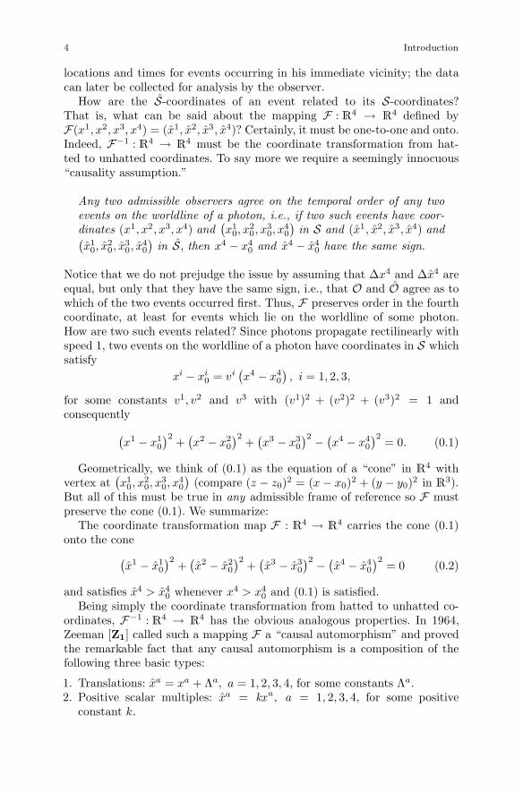
How are the S-coordinates of an event related to its S-coordinates?That is, what can be said about the mapping F : R4 → R4 defined byF(x1, x2, x3, x4) = (x1, x2, x3, x4)? Certainly, it must be one-to-one and onto.Indeed, F−1 : R4 → R4 must be the coordinate transformation from hat-ted to unhatted coordinates. To say more we require a seemingly innocuous“causality assumption.”
Any two admissible observers agree on the temporal order of any twoevents on the worldline of a photon, i.e., if two such events have coor-dinates (x1, x2, x3, x4) and
(x1
0, x20, x
30, x
40
)in S and (x1, x2, x3, x4) and(
x10, x
20, x
30, x
40
)in S, then x4 − x4
0 and x4 − x40 have the same sign.
Notice that we do not prejudge the issue by assuming that Δx4 and Δx4 areequal, but only that they have the same sign, i.e., that O and O agree as towhich of the two events occurred first. Thus, F preserves order in the fourthcoordinate, at least for events which lie on the worldline of some photon.How are two such events related? Since photons propagate rectilinearly withspeed 1, two events on the worldline of a photon have coordinates in S whichsatisfy
xi − xi0 = vi
(x4 − x4
0
), i = 1, 2, 3,
for some constants v1, v2 and v3 with (v1)2 + (v2)2 + (v3)2 = 1 andconsequently(
x1 − x10
)2+(x2 − x2
0
)2+(x3 − x3
0
)2 − (x4 − x40
)2= 0. (0.1)
Geometrically, we think of (0.1) as the equation of a “cone” in R4 withvertex at
(x1
0, x20, x
30, x
40
)(compare (z − z0)2 = (x − x0)2 + (y − y0)2 in R3).
But all of this must be true in any admissible frame of reference so F mustpreserve the cone (0.1). We summarize:
The coordinate transformation map F : R4 → R4 carries the cone (0.1)onto the cone(
x1 − x10
)2+(x2 − x2
0
)2+(x3 − x3
0
)2 − (x4 − x40
)2= 0 (0.2)
and satisfies x4 > x40 whenever x4 > x4
0 and (0.1) is satisfied.Being simply the coordinate transformation from hatted to unhatted co-
ordinates, F−1 : R4 → R4 has the obvious analogous properties. In 1964,Zeeman [Z1] called such a mapping F a “causal automorphism” and provedthe remarkable fact that any causal automorphism is a composition of thefollowing three basic types:
1. Translations: xa = xa + Λa, a = 1, 2, 3, 4, for some constants Λa.2. Positive scalar multiples: xa = kxa, a = 1, 2, 3, 4, for some positive
constant k.
Introduction 5
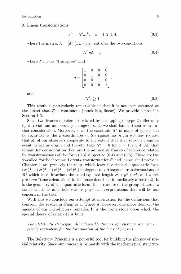
3. Linear transformations
xa = Λabx
b, a = 1, 2, 3, 4, (0.3)
where the matrix Λ = [Λab]a,b=1,2,3,4 satisfies the two conditions
ΛT ηΛ = η, (0.4)
where T means “transpose” and
η =
⎡⎢⎢⎣1 0 0 00 1 0 00 0 1 00 0 0 −1
⎤⎥⎥⎦ ,
andΛ4
4 ≥ 1. (0.5)
This result is particularly remarkable in that it is not even assumed atthe outset that F is continuous (much less, linear). We provide a proof inSection 1.6.
Since two frames of reference related by a mapping of type 2 differ onlyby a trivial and unnecessary change of scale we shall banish them from fur-ther consideration. Moreover, since the constants Λa in maps of type 1 canbe regarded as the S-coordinates of S’s spacetime origin we may requestthat all of our observers cooperate to the extent that they select a commonevent to act as origin and thereby take Λa = 0 for a = 1, 2, 3, 4. All thatremain for consideration then are the admissible frames of reference relatedby transformations of the form (0.3) subject to (0.4) and (0.5). These are theso-called “orthochronous Lorentz transformations” and, as we shall prove inChapter 1, are precisely the maps which leave invariant the quadratic form(x1)2 + (x2)2 + (x3)2 − (x4)2 (analogous to orthogonal transformations ofR3 which leave invariant the usual squared length x2 + y2 + z2) and whichpreserve “time orientation” in the sense described immediately after (0.2). Itis the geometry of this quadratic form, the structure of the group of Lorentztransformations and their various physical interpretations that will be ourconcern in the text.
With this we conclude our attempt at motivation for the definitions thatconfront the reader in Chapter 1. There is, however, one more item on theagenda of our introductory remarks. It is the cornerstone upon which thespecial theory of relativity is built.
The Relativity Principle: All admissible frames of reference are com-pletely equivalent for the formulation of the laws of physics.
The Relativity Principle is a powerful tool for building the physics of spe-cial relativity. Since our concern is primarily with the mathematical structure

6 Introduction
of the theory we shall have few occasions to call explicitly upon the Principleexcept for the physical interpretation of the mathematics and here it is vital.We regard the Relativity Principle primarily as an heuristic principle assert-ing that there are no “distinguished” admissible observers, i.e., that nonecan claim to have a privileged view of the universe. In particular, no suchobserver can claim to be “at rest” while the others are moving; they are allsimply in relative motion. We shall see that admissible observers can disagreeabout some rather startling things (e.g., whether or not two given events are“simultaneous”) and the Relativity Principle will prohibit us from preferringthe judgment of one to any of the others. Although we will not dwell onthe experimental evidence in favor of the Relativity Principle it should beobserved that its roots lie in such commonplace observations as the fact thata passenger in a (smooth, quiet) airplane travelling at constant groundspeedin a straight line cannot “feel” his motion relative to the earth, i.e., that nophysical effects are apparent in the plane which would serve to distinguish itfrom the (quasi-) admissible frame rigidly attached to the earth.
Our task then is to conduct a serious study of these “admissible framesof reference”. Before embarking on such a study, however, it is only fair toconcede that, in fact, no such thing exists. As is the case with any intellec-tual construct with which we attempt to model the physical universe, thenotion of an admissible frame of reference is an idealization, a rather fancifulgeneralization of circumstances which, to some degree of accuracy, are en-countered in the world. In particular, it has been found that the existence ofgravitational fields imposes severe restrictions on the “extent” (both in spaceand in time) of an admissible frame. Knowing this we will intentionally avoidthe difficulty (until Chapter 4) by restricting our attention to situations inwhich the effects of gravity are “negligible.”

Chapter 1
Geometrical Structure of M
1.1 Preliminaries
We denote by V an arbitrary vector space of dimension n ≥ 1 over the realnumbers. A bilinear form on V is a map g : V × V → R that is linearin each variable, i.e., such that g(a1v1 + a2v2, w) = a1g(v1, w) + a2g(v2, w)and g(v, a1w1 + a2w2) = a1g(v, w1) + a2g(v, w2) whenever the a’s are realnumbers and the v’s and w’s are elements of V . g is symmetric if g(w, v) =g(v, w) for all v and w and nondegenerate if g(v, w) = 0 for all w in V impliesv = 0. A nondegenerate, symmetric, bilinear form g is generally called aninner product and the image of (v, w) under g is often written v · w ratherthan g(v, w). The standard example is the usual inner product on Rn: if v =(v1, . . . , vn) and w = (w1, . . . , wn), then g(v, w) = v ·w = v1w1 + · · ·+vnwn.This particular inner product is positive definite, i.e., has the property that ifv �= 0, then g(v, v) > 0. Not all inner products share this property, however.
Exercise 1.1.1 Define a map g1 : Rn × Rn → R by g1(v, w) = v1w1 +v2w2 + · · ·+ vn−1wn−1 − vnwn. Show that g1 is an inner product and exhibitnonzero vectors v and w such that g1(v, v) = 0 and g1(w, w) < 0.
An inner product g for which v �= 0 implies g(v, v) < 0 is said to be negativedefinite, whereas if g is neither positive definite nor negative definite it is saidto be indefinite.
If g is an inner product on V , then two vectors v and w for whichg(v, w) = 0 are said to be g-orthogonal, or simply orthogonal if thereis no ambiguity as to which inner product is intended. If W is a sub-space of V , then the orthogonal complement W⊥ of W in V is defined byW⊥ = {v ∈ V : g(v, w) = 0 for all w ∈ W}.
Exercise 1.1.2 Show that W⊥ is a subspace of V .
The quadratic form associated with the inner product g on V is the mapQ : V → R defined by Q(v) = g(v, v) = v · v (often denoted v2). We ask
, : An Introduction , Applied Mathematical Sciences 92,
G.L. Naber The Geometry of Minkowski Spacetime to the Mathematics of the Special Theory of RelativityDOI 10.1007/978-1-4419-7838-7_ , © Springer Science+Business Media, LLC 2012
7
1
8 1 Geometrical Structure of M
the reader to show that distinct inner products on V cannot give rise to thesame quadratic form.
Exercise 1.1.3 Show that if g1 and g2 are two inner products on V whichsatisfy g1(v, v) = g2(v, v) for all v in V , then g1(v, w) = g2(v, w) for all v andw in V . Hint : The map g1 − g2 : V × V → R defined by (g1 − g2)(v, w) =g1(v, w)−g2(v, w) is bilinear and symmetric. Evaluate (g1−g2)(v+w, v+w).
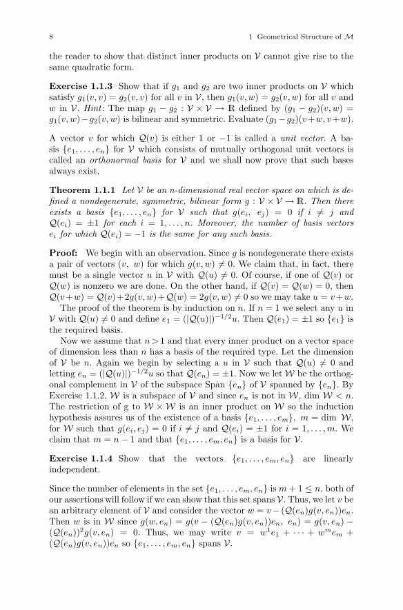
A vector v for which Q(v) is either 1 or −1 is called a unit vector. A ba-sis {e1, . . . , en} for V which consists of mutually orthogonal unit vectors iscalled an orthonormal basis for V and we shall now prove that such basesalways exist.
Theorem 1.1.1 Let V be an n-dimensional real vector space on which is de-fined a nondegenerate, symmetric, bilinear form g : V × V → R. Then thereexists a basis {e1, . . . , en} for V such that g(ei, ej) = 0 if i �= j andQ(ei) = ±1 for each i = 1, . . . , n. Moreover, the number of basis vectorsei for which Q(ei) = −1 is the same for any such basis.
Proof: We begin with an observation. Since g is nondegenerate there existsa pair of vectors (v, w) for which g(v, w) �= 0. We claim that, in fact, theremust be a single vector u in V with Q(u) �= 0. Of course, if one of Q(v) orQ(w) is nonzero we are done. On the other hand, if Q(v) = Q(w) = 0, thenQ(v+w) = Q(v)+2g(v, w)+Q(w) = 2g(v, w) �= 0 so we may take u = v+w.
The proof of the theorem is by induction on n. If n = 1 we select any u inV with Q(u) �= 0 and define e1 = (|Q(u)|)−1/2u. Then Q(e1) = ±1 so {e1} isthe required basis.
Now we assume that n > 1 and that every inner product on a vector spaceof dimension less than n has a basis of the required type. Let the dimensionof V be n. Again we begin by selecting a u in V such that Q(u) �= 0 andletting en = (|Q(u)|)−1/2u so that Q(en) = ±1. Now we let W be the orthog-onal complement in V of the subspace Span {en} of V spanned by {en}. ByExercise 1.1.2, W is a subspace of V and since en is not in W , dim W < n.The restriction of g to W × W is an inner product on W so the inductionhypothesis assures us of the existence of a basis {e1, . . . , em}, m = dim W ,for W such that g(ei, ej) = 0 if i �= j and Q(ei) = ±1 for i = 1, . . . , m. Weclaim that m = n − 1 and that {e1, . . . , em, en} is a basis for V .
Exercise 1.1.4 Show that the vectors {e1, . . . , em, en} are linearlyindependent.
Since the number of elements in the set {e1, . . . , em, en} is m + 1 ≤ n, both ofour assertions will follow if we can show that this set spans V . Thus, we let v bean arbitrary element of V and consider the vector w = v− (Q(en)g(v, en))en.Then w is in W since g(w, en) = g(v − (Q(en)g(v, en))en, en) = g(v, en) −(Q(en))2g(v, en) = 0. Thus, we may write v = w1e1 + · · · + wmem +(Q(en)g(v, en))en so {e1, . . . , em, en} spans V .

1.2 Minkowski Spacetime 9
To show that the number r of ei for which Q(ei) = −1 is the same forany orthonormal basis we proceed as follows: If r = 0 the result is clear sinceQ(v) ≥ 0 for every v in V , i.e., g is positive definite. If r > 0, then V willhave subspaces on which g is negative definite and so will have subspaces ofmaximal dimension on which g is negative definite. We will show that r is thedimension of any such maximal subspace W and thereby give an invariant(basis-independent) characterization of r. Number the basis elements so that{e1, . . . , er, er+1, . . . , en}, where Q(ei) = −1 for i = 1, . . . , r and Q(ei) = 1for i = r + 1, . . . , n. Let X = Span{e1, . . . , er} be the subspace of V spannedby {e1, . . . , er}. Then, since g is negative definite on X and dim X = r, wefind that r ≤ dim W . To show that r ≥ dim W as well we define a mapT : W → X as follows: If w =
∑ni=1 wiei is in W we let Tw =
∑ri=1 wiei.
Then T is obviously linear. Suppose w is such that Tw = 0. Then for eachi = 1, . . . , r, wi = 0. Thus,
Q(w) = g
⎛⎝ n∑i=r+1
wiei,
n∑j=r+1
wjej
⎞⎠ =n∑
i,j=r+1
g(ei, ej)wiwj =n∑
i=r+1
(wi)2
which is greater than or equal to zero. But g is negative definite on W sowe must have wi = 0 for i = r + 1, . . . , n, i.e., w = 0. Thus, the null spaceof T is {0} and T is therefore an isomorphism of W onto a subspace of X .Consequently, dimW ≤ dimX = r as required. �
The number r of ei in any orthonormal basis for g with Q(ei) = −1 is calledthe index of g. Henceforth we will assume that all orthonormal bases areindexed in such a way that these ei appear at the end of the list and so arenumbered as follows:
{e1, e2, . . . , en−r, en−r+1, . . . , en}
where Q(ei) = 1 for i = 1, 2, . . . , n−r and Q(ei) = −1 for i = n−r+1, . . . , n.Relative to such a basis if v = viei and w = wiei, then we have
g(v, w) = v1w1 + · · · + vn−rwn−r − vn−r+1wn−r+1 − · · · − vnwn.
1.2 Minkowski Spacetime
Minkowski spacetime is a 4-dimensional real vector space M on which isdefined a nondegenerate, symmetric, bilinear form g of index 1. The elementsof M will be called events and g is referred to as a Lorentz inner product onM. Thus, there exists a basis {e1, e2, e3, e4} for M with the property that ifv = vaea and w = waea, then
g(v, w) = v1w1 + v2w2 + v3w3 − v4w4.

10 1 Geometrical Structure of M
The elements of M are “events” and, as we suggested in the Introduction,are to be thought of intuitively as actual or physically possible point-events.An orthonormal basis {e1, e2, e3, e4} for M “coordinatizes” this event worldand is to be identified with a “frame of reference”. Thus, if x = x1e1 +x2e2 +x3e3 + x4e4, we regard the coordinates (x1, x2, x3, x4) of x relative to {ea}as the spatial (x1, x2, x3) and time (x4) coordinates supplied the event x bythe observer who presides over this reference frame. As we proceed with thedevelopment we will have occasion to expand upon, refine and add additionalelements to this basic physical interpretation, but, for the present, this willsuffice.
In the interest of economy we shall introduce a 4 × 4 matrix η defined by
η =
⎡⎢⎢⎣1 0 0 00 1 0 00 0 1 00 0 0 −1
⎤⎥⎥⎦ ,
whose entries will be denoted either ηab or ηab , the choice in any particularsituation being dictated by the requirements of the summation convention.Thus, ηab = ηab = 1 if a = b = 1, 2, 3, −1 if a = b = 4 and 0 otherwise.As a result we may write g(ea, eb) = ηab = ηab and, with the summationconvention, g(v, w) = ηabv
awb.Since our Lorentz inner product g on M is not positive definite there exist
nonzero vectors v in M for which g(v, v) = 0, e.g., v = e1 + e4 is one suchsince g(v, v) = Q(e1) + 2g(e1, e4) + Q(e4) = 1 + 0 − 1 = 0. Such vectors aresaid to be null (or lightlike, for reasons which will become clear shortly) andM actually has bases which consist exclusively of this type of vector.
Exercise 1.2.1 Construct a null basis for M, i.e., a set of four linearlyindependent null vectors.
Such a null basis cannot consist of mutually orthogonal vectors, however.
Theorem 1.2.1 Two nonzero null vectors v and w in M are orthogonal ifand only if they are parallel, i.e., iff there is a t in R such that v = tw.
Exercise 1.2.2 Prove Theorem 1.2.1. Hint : The Schwartz Inequality for R3
asserts that if x = (x1, x2, x3) and y = (y1, y2, y3), then
(x1y1 + x2y2 + x3y3)2 ≤ ((x1)2 + (x2)2 + (x3)2)((y1)2 + (y2)2 + (y3)2)
and that equality holds if and only if x and y are linearly dependent. �
Next consider two distinct events x0 and x for which the displacement vectorv = x − x0 from x0 to x is null, i.e., Q(v) = Q(x − x0) = 0. Relative to anyorthonormal basis {ea}, if x = xaea and x0 = xa
0ea, then(x1 − x1
0
)2+(x2 − x2
0
)2+(x3 − x3
0
)2 − (x4 − x40
)2= 0. (1.2.1)

1.2 Minkowski Spacetime 11
Fig. 1.2.1
But we have seen this before. It is precisely the condition which, in theIntroduction, we decided describes the relationship between two events thatlie on the worldline of some photon. For this reason, and because of the formalsimilarity between (1.2.1) and the equation of a right circular cone in R3, wedefine the null cone (or light cone) CN(x0) at x0 in M by
CN (x0) = {x ∈ M : Q(x − x0) = 0}
and picture it by suppressing the third spatial dimension x3 (see Figure 1.2.1).CN (x0) therefore consists of all those events in M that are “connectible tox0 by a light ray”. For any such event x (other than x0 itself) we define thenull worldline (or light ray) Rx0,x containing x0 and x by
Rx0,x = {x0 + t(x − x0) : t ∈ R}
and think of it as the worldline of that particular photon which experiencesboth x0 and x.
Exercise 1.2.3 Show that if Q(x − x0) = 0, then Rx,x0 = Rx0,x.
CN (x0) is just the union of all the light rays through x0. Indeed,
Theorem 1.2.2 Let x0 and x be two distinct events with Q(x−x0)= 0. Then
Rx0,x = CN (x0) ∩ CN(x). (1.2.2)
Proof: First let z = x0 + t(x − x0) be an element of Rx0,x. Then z − x0 =t(x−x0) so Q(z−x0) = t2Q(x−x0) = 0 so z is in CN (x0). With Exercise 1.2.3it follows in the same way that z is in CN (x) and so Rx0,x ⊆ CN (x0)∩CN (x).

12 1 Geometrical Structure of M
To prove the reverse containment we assume that z is in CN (x0) ∩ CN (x).Then each of the vectors z − x, z − x0 and x0 − x is null. But z − x0 =(z−x)−(x0−x) so 0 = Q(z−x0) = Q(z−x) − 2g(z−x, x0 − x)+Q(x0−x) =−2g(z−x, x0−x). Thus, g(z−x, x0 −x) = 0. If z = x we are done. If z �= x,then, since x �= x0, we may apply Theorem 1.2.1 to the orthogonal nullvectors z − x and x0 − x to obtain a t in R such that z − x = t(x0 − x) andit follows that z is in Rx0,x as required. �
For reasons which may not be apparent at the moment, but will becomeclear shortly, a vector v in M is said to be timelike if Q(v) < 0 and spacelikeif Q(v) > 0.
Exercise 1.2.4 Use an orthonormal basis for M to construct a few vectorsof each type.
If v is the displacement vector x − x0 between two events, then, relative toany orthonormal basis for M, Q(x − x0) < 0 becomes (Δx1)2 + (Δx2)2 +(Δx3)2 < (Δx4)2 (x − x0 is inside the null cone at x0). Thus, the (squared)spatial separation of the two events is less than the (squared) distance lightwould travel during the time lapse between the events (remember that x4 ismeasured in light travel time). If x−x0 is spacelike the inequality is reversed,we picture x−x0 outside the null cone at x0 and the spatial separation of x0
and x is so great that not even a photon travels quickly enough to experienceboth events.
If {e1, e2, e3, e4} and {e1, e2, e3, e4} are two orthonormal bases for M, thenthere is a unique linear transformation L : M → M such that L(ea) = ea foreach a = 1, 2, 3, 4. As we shall see, such a map “preserves the inner productof M”, i.e., is of the following type: A linear transformation L : M → M issaid to be an orthogonal transformation of M if g(Lx ,Ly) = g(x, y) for all xand y in M.
Exercise 1.2.5 Show that, since the inner product on M is nondegener-ate, an orthogonal transformation is necessarily one-to-one and therefore anisomorphism.
Lemma 1.2.3 Let L : M → M be a linear transformation. Then the fol-lowing are equivalent:
(a) L is an orthogonal transformation.(b) L preserves the quadratic form of M, i.e., Q(Lx) = Q(x) for all x in M.(c) L carries any orthonormal basis for M onto another orthonormal basis
for M.
Exercise 1.2.6 Prove Lemma 1.2.3. Hint : To prove that (b) implies (a)compute L(x + y) · L(x + y) − L(x − y) · L(x − y). �
Now let L :M→M be an orthogonal transformation of M and{e1, e2, e3, e4} an orthonormal basis for M. By Lemma 1.2.3, e1 =Le1, e2 =Le2, e3 = Le3 and e4 =Le4 also form an orthonormal basis for M. In
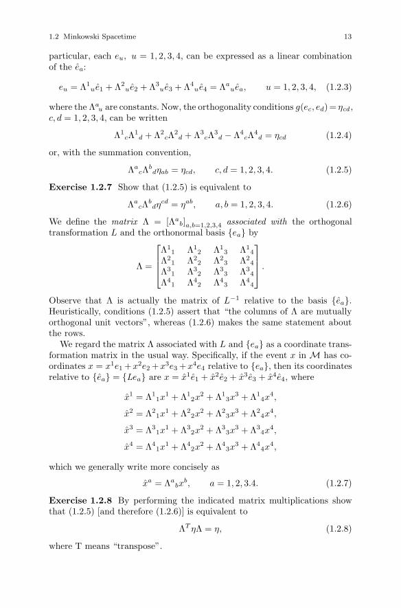
1.2 Minkowski Spacetime 13
particular, each eu, u = 1, 2, 3, 4, can be expressed as a linear combinationof the ea:
eu = Λ1ue1 + Λ2
ue2 + Λ3ue3 + Λ4
ue4 = Λauea, u = 1, 2, 3, 4, (1.2.3)
where the Λau are constants. Now, the orthogonality conditions g(ec, ed)= ηcd ,
c, d = 1, 2, 3, 4, can be written
Λ1cΛ1
d + Λ2cΛ2
d + Λ3cΛ3
d − Λ4cΛ4
d = ηcd (1.2.4)
or, with the summation convention,
ΛacΛb
dηab = ηcd, c, d = 1, 2, 3, 4. (1.2.5)
Exercise 1.2.7 Show that (1.2.5) is equivalent to
ΛacΛb
dηcd = ηab, a, b = 1, 2, 3, 4. (1.2.6)
We define the matrix Λ = [Λab]a,b=1,2,3,4 associated with the orthogonal
transformation L and the orthonormal basis {ea} by
Λ =
⎡⎢⎢⎣Λ1
1 Λ12 Λ1
3 Λ14
Λ21 Λ2
2 Λ23 Λ2
4
Λ31 Λ3
2 Λ33 Λ3
4
Λ41 Λ4
2 Λ43 Λ4
4
⎤⎥⎥⎦ .
Observe that Λ is actually the matrix of L−1 relative to the basis {ea}.Heuristically, conditions (1.2.5) assert that “the columns of Λ are mutuallyorthogonal unit vectors”, whereas (1.2.6) makes the same statement aboutthe rows.
We regard the matrix Λ associated with L and {ea} as a coordinate trans-formation matrix in the usual way. Specifically, if the event x in M has co-ordinates x = x1e1 +x2e2 +x3e3 +x4e4 relative to {ea}, then its coordinatesrelative to {ea} = {Lea} are x = x1e1 + x2e2 + x3e3 + x4e4, where
x1 = Λ11x
1 + Λ12x
2 + Λ13x
3 + Λ14x
4,
x2 = Λ21x
1 + Λ22x
2 + Λ23x
3 + Λ24x
4,
x3 = Λ31x
1 + Λ32x
2 + Λ33x
3 + Λ34x
4,
x4 = Λ41x
1 + Λ42x
2 + Λ43x
3 + Λ44x
4,
which we generally write more concisely as
xa = Λabx
b, a = 1, 2, 3.4. (1.2.7)
Exercise 1.2.8 By performing the indicated matrix multiplications showthat (1.2.5) [and therefore (1.2.6)] is equivalent to
ΛT ηΛ = η, (1.2.8)
where T means “transpose”.
14 1 Geometrical Structure of M
Notice that we have seen (1.2.8) before. It is just equation (0.4) of theIntroduction, which perhaps seems somewhat less mysterious now than itdid then. Indeed, (1.2.8) is now seen to be the condition that Λ is thematrix of a linear transformation which preserves the quadratic form ofM. In particular, if x − x0 is the displacement vector between two eventsfor which Q(x − x0) = 0, then both (Δx1)2 + (Δx2)2 + (Δx3)2 − (Δx4)2
and (Δx1)2 + (Δx2)2 + (Δx3)2 − (Δx4)2, where the Δxa are, from (1.2.7),Δxa = Λa
bΔxb, are zero. Physically, the two observers presiding over thehatted and unhatted reference frames agree that x0 and x are “connectibleby a light ray”, i.e., they agree on the speed of light.
Any 4× 4 matrix Λ that satisfies (1.2.8) is called a general (homogeneous)Lorentz transformation. At times we shall indulge in a traditional abuse ofterminology and refer to the coordinate transformation (1.2.7) as a Lorentztransformation. Since the orthogonal transformations of M are isomorphismsand therefore invertible, the matrix Λ associated with such an orthogonaltransformation must be invertible [also see (1.3.6)]. From (1.2.8) we find thatΛT ηΛ = η implies ΛT η = ηΛ−1 so that Λ−1 = η−1ΛT η or, since η−1 = η,
Λ−1 = ηΛT η. (1.2.9)
Exercise 1.2.9 Show that the set of all general (homogeneous) Lorentztransformations forms a group under matrix multiplication, i.e., that it isclosed under the formation of products and inverses. This group is called thegeneral (homogeneous) Lorentz group and we shall denote it by LGH .
We shall denote the entries in the matrix Λ−1 by Λab so that, by (1.2.9),⎡⎢⎢⎣
Λ11 Λ2
1 Λ31 Λ4
1
Λ12 Λ2
2 Λ32 Λ4
2
Λ13 Λ2
3 Λ33 Λ4
3
Λ14 Λ2
4 Λ34 Λ4
4
⎤⎥⎥⎦ =
⎡⎢⎢⎣Λ1
1 Λ21 Λ3
1 −Λ41
Λ12 Λ2
2 Λ32 −Λ4
2
Λ13 Λ2
3 Λ33 −Λ4
3
−Λ14 −Λ2
4 −Λ34 Λ4
4
⎤⎥⎥⎦ . (1.2.10)
Exercise 1.2.10 Show that
Λab = ηacη
bdΛcd, a, b = 1, 2, 3, 4, (1.2.11)
and similarlyΛa
b = ηacηbdΛcd, a, b = 1, 2, 3, 4. (1.2.12)
Since we have seen (Exercise 1.2.9) that Λ−1 is in LGH whenever Λ is it mustalso satisfy conditions analogous to (1.2.5) and (1.2.6), namely,
ΛacΛb
dηab = ηcd, c, d = 1, 2, 3, 4, (1.2.13)
andΛa
cΛbdηcd = ηab, a, b = 1, 2, 3, 4. (1.2.14)

1.3 The Lorentz Group 15
The analogues of (1.2.3) and (1.2.7) are
eu = Λuaea, u = 1, 2, 3, 4, (1.2.15)
andxb = Λa
bxa, b = 1, 2, 3, 4. (1.2.16)
1.3 The Lorentz Group
Observe that by setting c = d = 4 in (1.2.5) one obtains(Λ4
4
)2= 1 +(
Λ14
)2 +(Λ2
4
)2 +(Λ3
4
)2 so that, in particular,(Λ4
4
)2 ≥ 1. Consequently,
Λ44 ≥ 1 or Λ4
4 ≤ −1 (1.3.1)
An element Λ of LGH is said to be orthochronous if Λ44 ≥ 1 and
nonorthochronous if Λ44 ≤ −1. Nonorthochronous Lorentz transforma-
tions have certain unsavory characteristics which we now wish to expose.First, however, the following extremely important preliminary.
Theorem 1.3.1 Suppose that v is timelike and w is either timelike or nulland nonzero. Let {ea} be an orthonormal basis for M with v = vaea andw = waea. Then either
(a) v4w4 > 0, in which case g(v, w) < 0, or(b) v4w4 < 0, in which case g(v, w) > 0.
Proof: By assumption we have g(v, v)=(v1)2 + (v2)2 + (v3)2 − (v4)2 < 0and (w1)2 + (w2)2 + (w3)2−(w4)2 ≤ 0 so (v4w4)2 > ((v1)2 + (v2)2 +(v3)2)((w1)2 +(w2)2 +(w3)2) ≥ (v1w1 +v2w2 +v3w3)2, the second inequalityfollowing from the Schwartz Inequality for R3 (see Exercise 1.2.2). Thus, wefind that ∣∣v4w4
∣∣ > ∣∣v1w1 + v2w2 + v3w3∣∣,
so, in particular, v4w4 �= 0 and, moreover, g(v, w) �= 0. Suppose thatv4w4 > 0. Then v4w4 = |v4w4| > |v1w1+v2w2+v3w3| ≥ v1w1+v2w2 +v3w3
and so v1w1 + v2w2 + v3w3 − v4w4 < 0, i.e., g(v, w) < 0. On the other hand,if v4w4 < 0, then g(v, −w) < 0 so g(v, w) > 0. �
Corollary 1.3.2 If a nonzero vector in M is orthogonal to a timelike vector,then it must be spacelike.
We denote by τ the collection of all timelike vectors in M and define arelation ∼ on τ as follows: If v and w are in τ , then v ∼ w if and only ifg(v, w) < 0 (so that v4 and w4 have the same sign in any orthonormal basis).
16 1 Geometrical Structure of M
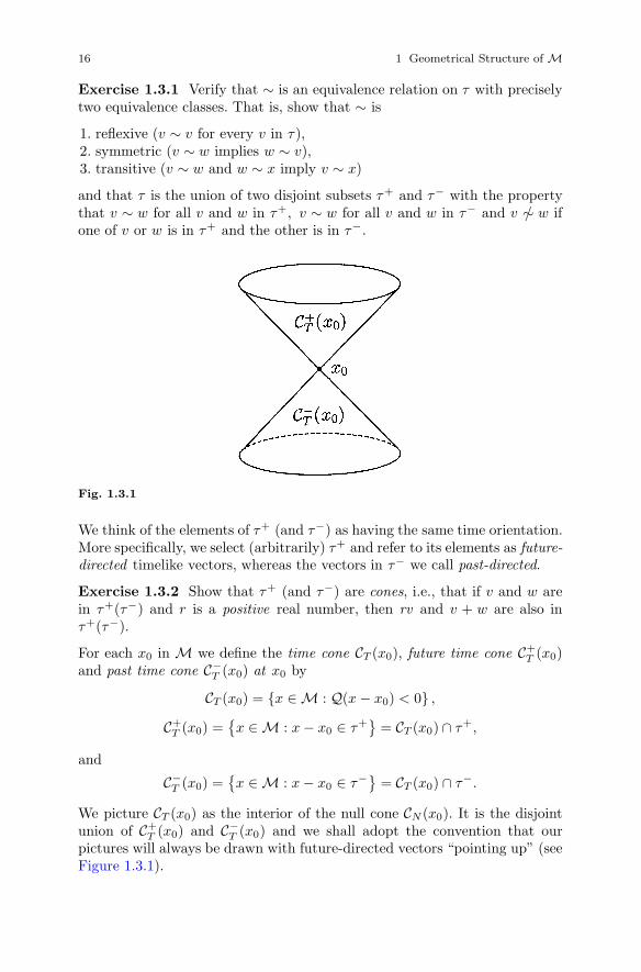
Exercise 1.3.1 Verify that ∼ is an equivalence relation on τ with preciselytwo equivalence classes. That is, show that ∼ is
1. reflexive (v ∼ v for every v in τ),2. symmetric (v ∼ w implies w ∼ v),3. transitive (v ∼ w and w ∼ x imply v ∼ x)
and that τ is the union of two disjoint subsets τ+ and τ− with the propertythat v ∼ w for all v and w in τ+, v ∼ w for all v and w in τ− and v /∼ w ifone of v or w is in τ+ and the other is in τ−.
Fig. 1.3.1
We think of the elements of τ+ (and τ−) as having the same time orientation.More specifically, we select (arbitrarily) τ+ and refer to its elements as future-directed timelike vectors, whereas the vectors in τ− we call past-directed.
Exercise 1.3.2 Show that τ+ (and τ−) are cones, i.e., that if v and w arein τ+(τ−) and r is a positive real number, then rv and v + w are also inτ+(τ−).
For each x0 in M we define the time cone CT (x0), future time cone C+T (x0)
and past time cone C−T (x0) at x0 by
CT (x0) = {x ∈ M : Q(x − x0) < 0} ,
C+T (x0) =
{x ∈ M : x − x0 ∈ τ+
}= CT (x0) ∩ τ+,
and
C−T (x0) =
{x ∈ M : x − x0 ∈ τ−} = CT (x0) ∩ τ−.
We picture CT (x0) as the interior of the null cone CN (x0). It is the disjointunion of C+
T (x0) and C−T (x0) and we shall adopt the convention that our
pictures will always be drawn with future-directed vectors “pointing up” (seeFigure 1.3.1).

1.3 The Lorentz Group 17
We wish to extend the notion of past- and future-directed to nonzero nullvectors as well. First we observe that if n is a nonzero null vector, thenn · v has the same sign for all v in τ+. To see this we suppose that thereexist vectors v1 and v2 in τ+ such that n · v1 < 0 and n · v2 > 0. We mayassume that |n · v1| = n · v2 since if this is not the case we can replacev1 by (n · v2/|n · v1|)v1, which is still in τ+ by Exercise 1.3.2 and satisfiesg(n, (n ·v2/|n ·v1|)v1) = (n ·v2/|n ·v1|)g(n, v1) = −n ·v2. Thus, n ·v1 = −n ·v2
so n·v1+n·v2 = 0 and therefore n·(v1+v2) = 0. But, again by Exercise 1.3.2,v1 + v2 is in τ+ and so, in particular, is timelike. Since n is nonzero and nullthis contradicts Corollary 1.3.2. Thus, we may say that a nonzero null vectorn is future-directed if n · v < 0 for all v in τ+ and past-directed if n · v > 0 forall v in τ+.
Exercise 1.3.3 Show that two nonzero null vectors n1 and n2 have the sametime orientation (i.e., are both past-directed or both future-directed) if andonly if n4
1 and n42 have the same sign relative to any orthonormal basis for M.
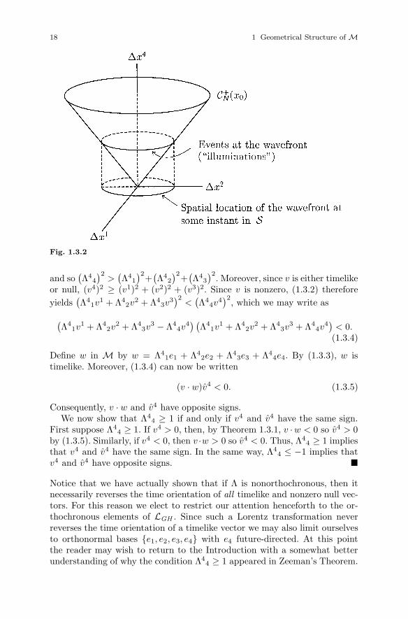
For any x0 in M we define the future null cone at x0 by C+N (x0) =
{x ∈ CN(x0) : x − x0 is future-directed} and the past null cone at x0 byC−
N (x0) = {x ∈ CN(x0) : x − x0 is past-directed}. Physically, event x is inC+
N (x0) if x0 and x respectively can be regarded as the emission and recep-tion of a light signal. Consequently, C+
N (x0) may be thought of as the historyin spacetime of a spherical electromagnetic wave (photons in all directions)whose emission event is x0 (see Figure 1.3.2).
The disagreeable nature of nonorthochronous Lorentz transformations isthat they always reverse time orientations (and so presumably relate referenceframes in which someone’s clock is running backwards).
Theorem 1.3.3 Let Λ = [Λab]a,b=1,2,3,4 be an element of LGH and
{ea}a=1,2,3,4 an orthonormal basis for M. Then the following are equivalent:
(a) Λ is orthochronous.(b) Λ preserves the time orientation of all nonzero null vectors, i.e., if v =
vaea is a nonzero null vector, then the numbers v4 and v4 = Λ4bv
b havethe same sign.
(c) Λ preserves the time orientation of all timelike vectors.
Proof: Let v = vaea be a vector which is either timelike or null and nonzero.By the Schwartz Inequality for R3 we have
(Λ4
1v1 + Λ4
2v2 + Λ4
3v3)2 ≤
(3∑
i=1
(Λ4
i
)2)( 3∑i=1
(vi)2)
. (1.3.2)
Now, by (1.2.6) with a = b = 4, we have(Λ4
1
)2+(Λ4
2
)2+(Λ4
3
)2 − (Λ44
)2= −1 (1.3.3)
18 1 Geometrical Structure of M
Fig. 1.3.2
and so(Λ4
4
)2>(Λ4
1
)2+(Λ4
2
)2+(Λ4
3
)2. Moreover, since v is either timelikeor null, (v4)2 ≥ (v1)2 + (v2)2 + (v3)2. Since v is nonzero, (1.3.2) thereforeyields
(Λ4
1v1 + Λ4
2v2 + Λ4
3v3)2
<(Λ4
4v4)2
, which we may write as(Λ4
1v1 + Λ4
2v2 + Λ4
3v3 − Λ4
4v4) (
Λ41v
1 + Λ42v
2 + Λ43v
3 + Λ44v
4)
< 0.(1.3.4)
Define w in M by w = Λ41e1 + Λ4
2e2 + Λ43e3 + Λ4
4e4. By (1.3.3), w istimelike. Moreover, (1.3.4) can now be written
(v · w)v4 < 0. (1.3.5)
Consequently, v · w and v4 have opposite signs.We now show that Λ4
4 ≥ 1 if and only if v4 and v4 have the same sign.First suppose Λ4
4 ≥ 1. If v4 > 0, then, by Theorem 1.3.1, v ·w < 0 so v4 > 0by (1.3.5). Similarly, if v4 < 0, then v ·w > 0 so v4 < 0. Thus, Λ4
4 ≥ 1 impliesthat v4 and v4 have the same sign. In the same way, Λ4
4 ≤ −1 implies thatv4 and v4 have opposite signs. �
Notice that we have actually shown that if Λ is nonorthochronous, then itnecessarily reverses the time orientation of all timelike and nonzero null vec-tors. For this reason we elect to restrict our attention henceforth to the or-thochronous elements of LGH . Since such a Lorentz transformation neverreverses the time orientation of a timelike vector we may also limit ourselvesto orthonormal bases {e1, e2, e3, e4} with e4 future-directed. At this pointthe reader may wish to return to the Introduction with a somewhat betterunderstanding of why the condition Λ4
4 ≥ 1 appeared in Zeeman’s Theorem.
1.3 The Lorentz Group 19
There is yet one more restriction we would like to impose on ourLorentz transformations. Observe that taking determinants on both sidesof (1.2.8) yields (det ΛT )(det η)(det Λ) = det η so that, since det ΛT =det Λ, (det Λ)2 = 1 and therefore
detΛ = 1 or detΛ = −1. (1.3.6)
We shall say that a Lorentz transformation Λ is proper if det Λ = 1 andimproper if detΛ = −1.
Exercise 1.3.4 Show that an orthochronous Lorentz transformation is im-proper if and only if it is of the form⎡⎢⎢⎣
−1 0 0 00 1 0 00 0 1 00 0 0 1
⎤⎥⎥⎦Λ, (1.3.7)
where Λ is proper and orthochronous.
Notice that the matrix on the left in (1.3.7) is an orthochronous Lorentztransformation and, as a coordinate transformation, has the effect of chang-ing the sign of the first spatial coordinate, i.e., of reversing the spatial orienta-tion (left-handed to right-handed or right-handed to left-handed). Since thereseems to be no compelling reason to make such a change we intend to restrictour attention to the set L of proper, orthochronous Lorentz transformations.Having done so we may further limit the orthonormal bases we consider byselecting an orientation for the spatial coordinate axes. Specifically, we de-fine an admissible basis for M to be an orthonormal basis {e1, e2, e3, e4}with e4 timelike and future-directed and {e1, e2, e3} spacelike and “right-handed”, i.e., satisfying e1 × e2 · e3 = 1 (since the restriction of g to thespan of {e1, e2, e3} is the usual dot product on R3, the cross product and dotproduct here are the familiar ones from vector calculus). At this point wefully identify an “admissible basis” with an “admissible frame of reference”as discussed in the Introduction. Any two such bases (frames) are related bya proper, orthochronous Lorentz transformation.
Exercise 1.3.5 Show that the set L of proper, orthochronous Lorentz trans-formations is a subgroup of LGH , i.e., that it is closed under the formationof products and inverses.
Generally, we shall refer to L simply as the Lorentz group and its elementsas Lorentz transformations with the understanding that they are all properand orthochronous. Occasionally it is convenient to enlarge the group of coor-dinate transformations to include spacetime translations (see the statementof Zeeman’s Theorem in the Introduction), thereby obtaining the so-calledinhomogeneous Lorentz group or Poincare group. Physically, this amounts toallowing “admissible” observers to use different spacetime origins.

20 1 Geometrical Structure of M
The Lorentz group L has an important subgroup R consisting of thoseR = [Ra
b] of the form
R =
⎡⎢⎢⎣0[
Rij
]00
0 0 0 1
⎤⎥⎥⎦ ,
where [Rij ]i,j=1,2,3 is a unimodular orthogonal matrix, i.e., satisfies
det[Rij ] = 1 and [Ri
j ]T = [Rij ]−1. Observe that the orthogonality con-
ditions (1.2.5) are clearly satisfied by such an R and that, moreover, R44 = 1
and detR = det[Rij ] = 1 so that R is indeed in L. The coordinate transfor-
mation associated with R corresponds physically to a rotation of the spatialcoordinate axes within a given frame of reference. For this reason R is calledthe rotation subgroup of L and its elements are called rotations in L.
Lemma 1.3.4 Let Λ = [Λab]a,b=1,2,3,4 be a proper, orthochronous Lorentz
transformation. Then the following are equivalent:
(a) Λ is a rotation,(b) Λ1
4 = Λ24 = Λ3
4 = 0,(c) Λ4
1 = Λ42 = Λ4
3 = 0,(d) Λ4
4 = 1.
Proof: Set c = d = 4 in (1.2.5) to obtain(Λ1
4
)2+(Λ2
4
)2+(Λ3
4
)2 − (Λ44
)2= −1. (1.3.8)
Similarly, with a = b = 4, (1.2.6) becomes(Λ4
1
)2+(Λ4
2
)2+(Λ4
3
)2 − (Λ44
)2= −1. (1.3.9)
The equivalence of (b), (c) and (d) now follows immediately from (1.3.8) and(1.3.9) and the fact that Λ is assumed orthochronous. Since a rotation in Lsatisfies (b), (c) and (d) by definition, all that remains is to show that if Λsatisfies one (and therefore all) of these conditions, then
[Λi
j
]i,j=1,2,3
is aunimodular orthogonal matrix.
Exercise 1.3.6 Complete the proof. �
Exercise 1.3.7 Use Lemma 1.3.4 to show that R is a subgroup of L, i.e.,that it is closed under the formation of inverses and products.
Exercise 1.3.8 Show that an element of L has the same fourth row as[Λa
b]a,b=1,2,3,4 if and only if it can be obtained from [Λab] by multiplying on
the left by some rotation in L. Similarly, an element of L has the same fourthcolumn as [Λa
b] if and only if it can be obtained from [Λab] by multiplying
on the right by an element of R.
1.3 The Lorentz Group 21
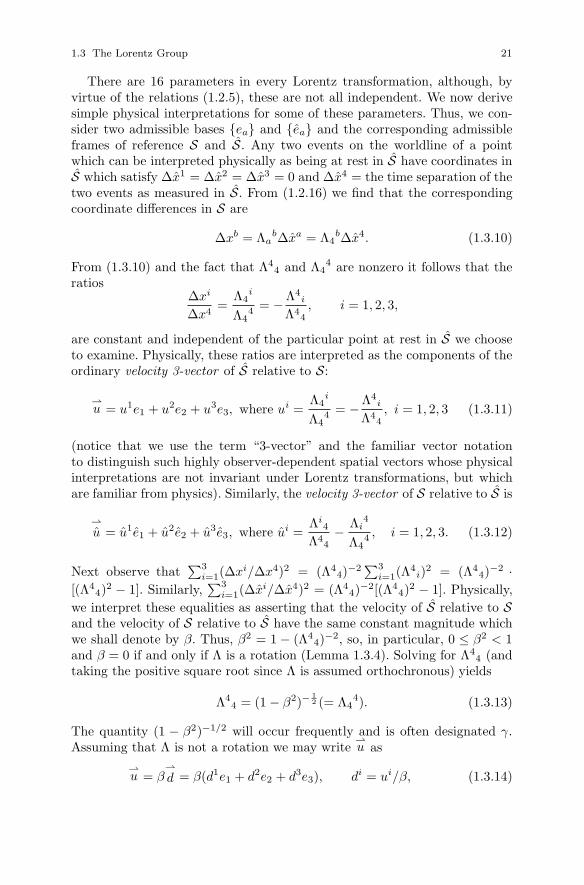
There are 16 parameters in every Lorentz transformation, although, byvirtue of the relations (1.2.5), these are not all independent. We now derivesimple physical interpretations for some of these parameters. Thus, we con-sider two admissible bases {ea} and {ea} and the corresponding admissibleframes of reference S and S. Any two events on the worldline of a pointwhich can be interpreted physically as being at rest in S have coordinates inS which satisfy Δx1 = Δx2 = Δx3 = 0 and Δx4 = the time separation of thetwo events as measured in S. From (1.2.16) we find that the correspondingcoordinate differences in S are
Δxb = ΛabΔxa = Λ4
bΔx4. (1.3.10)
From (1.3.10) and the fact that Λ44 and Λ4
4 are nonzero it follows that theratios
Δxi
Δx4=
Λ4i
Λ44
= −Λ4i
Λ44, i = 1, 2, 3,
are constant and independent of the particular point at rest in S we chooseto examine. Physically, these ratios are interpreted as the components of theordinary velocity 3-vector of S relative to S:
⇀u = u1e1 + u2e2 + u3e3, where ui =
Λ4i
Λ44 = −Λ4
i
Λ44, i = 1, 2, 3 (1.3.11)
(notice that we use the term “3-vector” and the familiar vector notationto distinguish such highly observer-dependent spatial vectors whose physicalinterpretations are not invariant under Lorentz transformations, but whichare familiar from physics). Similarly, the velocity 3-vector of S relative to S is
⇀
u = u1e1 + u2e2 + u3e3, where ui =Λi
4
Λ44− Λi
4
Λ44 , i = 1, 2, 3. (1.3.12)
Next observe that∑3
i=1(Δxi/Δx4)2 = (Λ44)−2∑3
i=1(Λ4i)2 = (Λ4
4)−2 ·[(Λ4
4)2 − 1]. Similarly,∑3
i=1(Δxi/Δx4)2 = (Λ44)−2[(Λ4
4)2 − 1]. Physically,we interpret these equalities as asserting that the velocity of S relative to Sand the velocity of S relative to S have the same constant magnitude whichwe shall denote by β. Thus, β2 = 1 − (Λ4
4)−2, so, in particular, 0 ≤ β2 < 1and β = 0 if and only if Λ is a rotation (Lemma 1.3.4). Solving for Λ4
4 (andtaking the positive square root since Λ is assumed orthochronous) yields
Λ44 = (1 − β2)−
12 (= Λ4
4). (1.3.13)
The quantity (1 − β2)−1/2 will occur frequently and is often designated γ.Assuming that Λ is not a rotation we may write
⇀u as
⇀u = β
⇀
d = β(d1e1 + d2e2 + d3e3), di = ui/β, (1.3.14)
22 1 Geometrical Structure of M
where⇀
d is the direction 3-vector of S relative to S and the di are interpretedas the direction cosines of the directed line segment in
∑along which the
observer in S sees∑
moving. Similarly,⇀
u = β⇀
d = β(d1e1 + d2e2 + d3e3), di = ui/β. (1.3.15)
Exercise 1.3.9 Show that the di are the components of the normalizedprojection of e4 onto the subspace spanned by {e1, e2, e3}, i.e., that
di =
⎛⎝ 3∑j=1
(e4 · ej)2
⎞⎠− 12
(e4 · ei), i = 1, 2, 3, (1.3.16)
and similarly
di =
⎛⎝ 3∑j=1
(e4 · ej)2
⎞⎠− 12
(e4 · ei), i = 1, 2, 3. (1.3.17)
Exercise 1.3.10 Show that e4 = γ(β⇀
d +e4) and, similarly, e4 = γ(β⇀
d + e4)and notice that it follows from these that e4 · e4 = e4 · e4 = −γ.
Comparing (1.3.11) and (1.3.14) and using (1.3.13) we obtain
Λ4i = −Λ4
i = β(1 − β2)−12 di, i = 1, 2, 3, (1.3.18)
and similarly
Λi4 = −Λi
4 = β(1 − β2)−12 di, i = 1, 2, 3. (1.3.19)
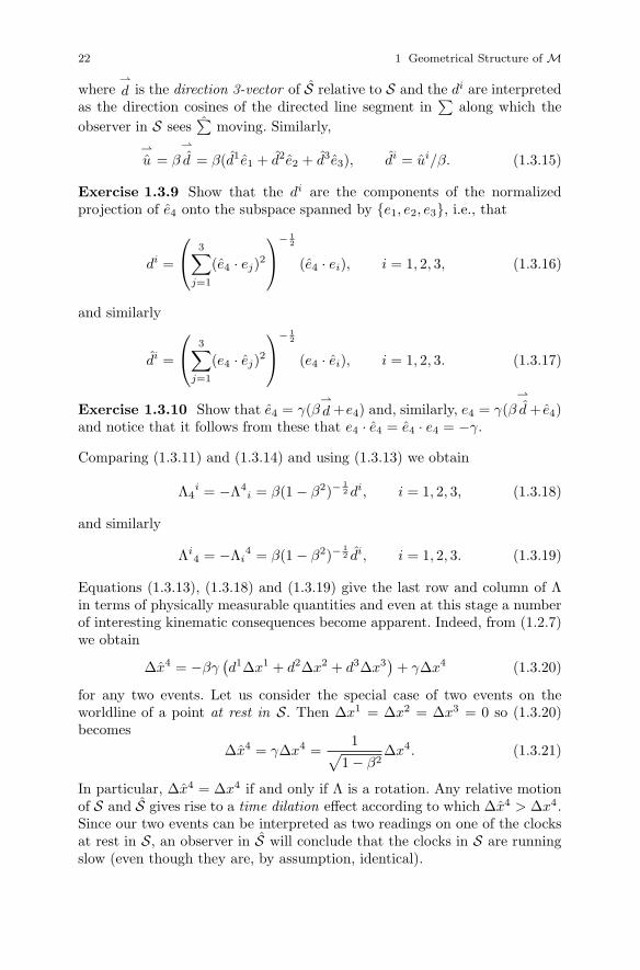
Equations (1.3.13), (1.3.18) and (1.3.19) give the last row and column of Λin terms of physically measurable quantities and even at this stage a numberof interesting kinematic consequences become apparent. Indeed, from (1.2.7)we obtain
Δx4 = −βγ(d1Δx1 + d2Δx2 + d3Δx3
)+ γΔx4 (1.3.20)
for any two events. Let us consider the special case of two events on theworldline of a point at rest in S. Then Δx1 = Δx2 = Δx3 = 0 so (1.3.20)becomes
Δx4 = γΔx4 =1√
1 − β2Δx4. (1.3.21)
In particular, Δx4 = Δx4 if and only if Λ is a rotation. Any relative motionof S and S gives rise to a time dilation effect according to which Δx4 > Δx4.Since our two events can be interpreted as two readings on one of the clocksat rest in S, an observer in S will conclude that the clocks in S are runningslow (even though they are, by assumption, identical).
1.3 The Lorentz Group 23
Exercise 1.3.11 Show that this time dilation effect is entirely symmetrical,i.e., that for two events with Δx1 = Δx2 = Δx3 = 0,
Δx4 = γΔx4 =1√
1 − β2Δx4. (1.3.22)
We shall return to this phenomenon of time dilation in much greater detailafter we have introduced a geometrical construction for picturing it. Never-theless, we should point out at the outset that it is in no sense an illusion;it is quite “real” and can manifest itself in observable phenomena. One suchinstance occurs in the study of cosmic rays (“showers” of various types ofelementary particles from space which impact the earth). Certain types ofmesons that are encountered in cosmic radiation are so short-lived (at rest)that even if they could travel at the speed of light (which they cannot) thetime required to traverse our atmosphere would be some ten times their nor-mal life span. They should not be able to reach the earth, but they do. Timedilation, in a sense, “keeps them young”. The meson’s notion of time is notthe same as ours. What seems a normal lifetime to the meson appears muchlonger to us. It is well to keep in mind also that we have been rather vagueabout what we mean by a “clock”. Essentially any phenomenon involving ob-servable change (successive readings on a Timex, vibrations of an atom, thelifetime of a meson, or a human being) is a “clock” and is therefore subjectto the effects of time dilation. Of course, the effects will be negligibly smallunless β is quite close to 1 (the speed of light). On the other hand, as β → 1,(1.3.21) shows that Δx4 → ∞ so that as speeds approach that of light theeffects become infinitely great.
Another special case of (1.3.20) is also of interest. Let us suppose that ourtwo events are judged simultaneous in S, i.e., that Δx4 = 0. Then
Δx4 = −βγ(d1Δx1 + d2Δx2 + d3Δx3
). (1.3.23)
Again assuming that β �= 0 we find that, in general, Δx4 will not be zero,i.e., that the two events will not be judged simultaneous in S. Indeed, S andS will agree on the simultaneity of these two events if and only if the spatiallocations of the events in
∑bear a very special relation to the direction in∑
along which∑
is moving, namely,
d1Δx1 + d2Δx2 + d3Δx3 = 0 (1.3.24)
(the displacement vector in∑
between the locations of the two events iseither zero or nonzero and perpendicular to the direction of
∑’s motion in∑
). Otherwise, Δx4 �= 0 and we have an instance of what is called therelativity of simultaneity. Notice, incidentally, that such disagreement canarise only for spatially separated events. More precisely, if in some admissibleframe S two events x and x0 are simultaneous and occur at the same spatiallocation, then Δxa = 0 for a = 1, 2, 3, 4 so x − x0 = 0. Since the Lorentztransformations are linear it follows that Δxa = 0 for a = 1, 2, 3, 4, i.e., theevents are also simultaneous and occur at the same spatial location in S.Again, we will return to this phenomenon in much greater detail shortly.
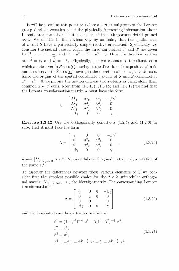
24 1 Geometrical Structure of M
It will be useful at this point to isolate a certain subgroup of the Lorentzgroup L which contains all of the physically interesting information aboutLorentz transformations, but has much of the unimportant detail prunedaway. We do this in the obvious way by assuming that the spatial axesof S and S have a particularly simple relative orientation. Specifically, weconsider the special case in which the direction cosines di and di are givenby d1 = 1, d1 = −1 and d2 = d2 = d3 = d3 = 0. Thus, the direction vectors
are⇀
d = e1 and⇀
d = −e1. Physically, this corresponds to the situation inwhich an observer in S sees
∑moving in the direction of the positive x1-axis
and an observer in S sees∑
moving in the direction of the negative x1-axis.Since the origins of the spatial coordinate systems of S and S coincided atx4 = x4 = 0, we picture the motion of these two systems as being along theircommon x1-, x1-axis. Now, from (1.3.13), (1.3.18) and (1.3.19) we find thatthe Lorentz transformation matrix Λ must have the form
Λ =
⎡⎢⎢⎣Λ1
1 Λ12 Λ1
3 −βγΛ2
1 Λ22 Λ2
3 0Λ3
1 Λ32 Λ3
3 0−βγ 0 0 γ
⎤⎥⎥⎦ .
Exercise 1.3.12 Use the orthogonality conditions (1.2.5) and (1.2.6) toshow that Λ must take the form
Λ =
⎡⎢⎢⎣γ 0 0 −βγ0 Λ2
2 Λ23 0
0 Λ32 Λ3
3 0−βγ 0 0 γ
⎤⎥⎥⎦ , (1.3.25)
where[Λi
j
]i,j=2,3
is a 2× 2 unimodular orthogonal matrix, i.e., a rotation ofthe plane R2.
To discover the differences between these various elements of L we con-sider first the simplest possible choice for the 2 × 2 unimodular orthogo-nal matrix [Λi
j ]i,j=2,3, i.e., the identity matrix. The corresponding Lorentztransformation is
Λ =
⎡⎢⎢⎣γ 0 0 −βγ0 1 0 00 0 1 0
−βγ 0 0 γ
⎤⎥⎥⎦ (1.3.26)
and the associated coordinate transformation is
x1 = (1 − β2)−12 x1 − β(1 − β2)−
12 x4,
x2 = x2,
x3 = x3,
x4 = −β(1 − β2)−12 x1 + (1 − β2)−
12 x4.
(1.3.27)
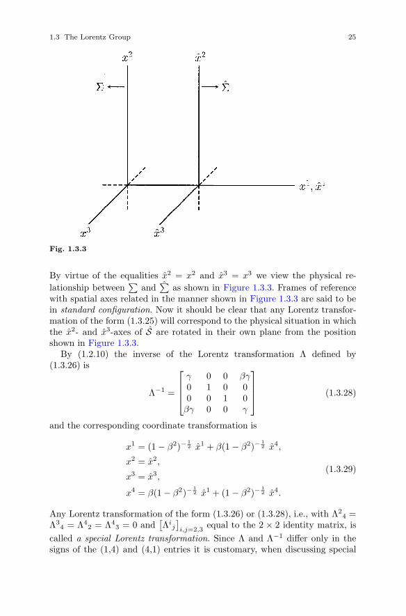
1.3 The Lorentz Group 25
Fig. 1.3.3
By virtue of the equalities x2 = x2 and x3 = x3 we view the physical re-lationship between
∑and∑
as shown in Figure 1.3.3. Frames of referencewith spatial axes related in the manner shown in Figure 1.3.3 are said to bein standard configuration. Now it should be clear that any Lorentz transfor-mation of the form (1.3.25) will correspond to the physical situation in whichthe x2- and x3-axes of S are rotated in their own plane from the positionshown in Figure 1.3.3.
By (1.2.10) the inverse of the Lorentz transformation Λ defined by(1.3.26) is
Λ−1 =
⎡⎢⎢⎣γ 0 0 βγ0 1 0 00 0 1 0
βγ 0 0 γ
⎤⎥⎥⎦ (1.3.28)
and the corresponding coordinate transformation is
x1 = (1 − β2)−12 x1 + β(1 − β2)−
12 x4,
x2 = x2,
x3 = x3,
x4 = β(1 − β2)−12 x1 + (1 − β2)−
12 x4.
(1.3.29)
Any Lorentz transformation of the form (1.3.26) or (1.3.28), i.e., with Λ24 =
Λ34 = Λ4
2 = Λ43 = 0 and
[Λi
j
]i,j=2,3
equal to the 2 × 2 identity matrix, iscalled a special Lorentz transformation. Since Λ and Λ−1 differ only in thesigns of the (1,4) and (4,1) entries it is customary, when discussing special
26 1 Geometrical Structure of M
Lorentz transformations, to allow −1 < β < 1. By choosing β > 0 whenΛ1
4 < 0 and β < 0 when Λ14 > 0 all special Lorentz transformations can be
written in the form (1.3.26) and we shall henceforth adopt this convention.For each real number β with −1 < β < 1 we therefore define γ = γ(β) =(1 − β2)−1/2 and
Λ(β) =
⎡⎢⎢⎣γ 0 0 −βγ0 1 0 00 0 1 0
−βγ 0 0 γ
⎤⎥⎥⎦ .
The matrix Λ(β) is often called a boost in the x1-direction.
Exercise 1.3.13 Define matrices which represent boosts in the x2- and x3-directions. One can define a boost in an arbitrary direction by first rotating,say, the positive x1-axis into that direction and then applying Λ(β).
Exercise 1.3.14 Suppose −1 < β1 ≤ β2 < 1. Show that
(a)∣∣∣∣ β1 + β2
1 + β1β2
∣∣∣∣ < 1. Hint : Show that if a is a constant satisfying −1 < a < 1,
then the function f(x) =x + a
1 + axis increasing on −1 ≤ x ≤ 1.
(b) Λ(β1)Λ(β2) = Λ(
β1 + β2
1 + β1β2
). (1.3.30)
It follows from Exercise 1.3.14 that the composition of two boosts in thex1-direction is another boost in the x1-direction. Since Λ−1(β) = Λ(−β) thecollection of all such special Lorentz transformations forms a subgroup of L.We point out, however, that the composition of two boosts in two differentdirections is, in general, not equivalent to a single boost in any direction.
By referring the three special Lorentz transformations Λ(β1), Λ(β2) andΛ(β1)Λ(β2) to the corresponding admissible frames of reference one arrivesat the following physical interpretation of (1.3.30): If the speed of S relative
to S is β1 and the speed of ˆS relative to S is β2, then the speed of ˆS relativeto S is not β1 + β2 as one might expect, but rather
β1 + β2
1 + β1β2,
which is always less than β1 + β2 provided β1β2 �= 0. Equation (1.3.30) isgenerally known as the relativistic addition of velocities formula. It, togetherwith part (a) of Exercise 1.3.14, confirms the suspicion, already indicated bythe behavior of (1.3.21) as β → 1, that the relative speed of two admissibleframes of reference is always less than that of light (that is, 1). Since any ma-terial object can be regarded as at rest in some admissible frame we concludethat such an object cannot attain (or exceed) the speed of light relative toan admissible frame.
1.3 The Lorentz Group 27
Despite this “nonadditivity” of speeds in relativity it is often convenient tomeasure speeds with an alternative “velocity parameter” θ that is additive.An analogous situation occurs in plane Euclidean geometry where one hasthe option of describing the relative orientation of two Cartesian coordinatesystems by means of angles (which are additive) or slopes (which are not).What we would like then is a measure θ of relative velocities with the propertythat if θ1 is the velocity parameter of S relative to S and θ2 is the velocityparameter of ˆS relative to S, then the velocity parameter of ˆS relative to S,is θ1 + θ2. Since θ is to measure relative speed, β will be some one-to-onefunction of θ, say, β = f(θ). Additivity and (1.3.30) require that f satisfythe functional equation
f(θ1 + θ2) =f(θ1) + f(θ2)
1 + f(θ1) f(θ2). (1.3.31)
Being reminiscent of the sum formula for the hyperbolic tangent, (1.3.31)suggests the change of variable
β = tanh θ or θ = tanh−1 β. (1.3.32)
Observe that tanh−1 is a one-to-one differentiable function of (−1, 1) ontoR with the property that β → ±1 implies θ → ±∞, i.e., the speed of lighthas infinite velocity parameter. If this change of variable seems to have beenpulled out of the air it may be comforting to have a uniqueness theorem.
Exercise 1.3.15 Show that there is exactly one differentiable function β =f(θ) on R (namely, tanh) which satisfies (1.3.31) and the requirement that,for small speeds, β and θ are nearly equal, i.e., that
limθ→0
f(θ)θ
= 1.
Hint : Show that such an f necessarily satisfies the initial value problemf ′(θ) = 1−(f(θ))2, f(0) = 0 and appeal to the standard Uniqueness Theoremfor solutions to such problems. Solve the problem to show that f(θ) = tanh θ.
Exercise 1.3.16 Show that if β = tanh θ, then the hyperbolic form of theLorentz transformation Λ(β) is
L(θ) =
⎡⎢⎢⎣cosh θ 0 0 − sinh θ
0 1 0 00 0 1 0
− sinh θ 0 0 cosh θ
⎤⎥⎥⎦ .
Earlier we suggested that all of the physically interesting behavior ofproper, orthochronous Lorentz transformations is exhibited by the specialLorentz transformations. What we had in mind is the following theoremwhich asserts that any element of L differs from some L(θ) only by at mosttwo rotations. This result will also be important in Section 1.7.

28 1 Geometrical Structure of M
Theorem 1.3.5 Let Λ = [Λab]a,b=1,2,3,4 be a proper, orthochronous Lorentz
transformation. Then there exists a real number θ and two rotations R1 andR2 in R such that Λ = R1L(θ)R2.
Proof: Suppose first that Λ14 = Λ2
4 = Λ34 = 0. Then, by Lemma 1.3.4,
Λ is itself a rotation and so we may take R1 = Λ, θ = 0 and R2 to bethe 4 × 4 identity matrix. Consequently, we may assume that the vector(Λ1
4, Λ24, Λ3
4
)in R3 is nonzero. Dividing by its magnitude in R3 gives a
vector⇀u1 = (α1, α2, α3) of unit length in R3. Let
⇀u2 = (β1, β2, β3) and
⇀u3 = (γ1, γ2, γ3) be vectors in R3 such that {⇀
u1,⇀u 2,
⇀u 3} is an orthonormal
basis for R3. Then ⎡⎣α1 α2 α3
β1 β2 β3
γ1 γ2 γ3
⎤⎦is an orthogonal matrix in R3 which, by a suitable ordering of the basis{⇀u1,
⇀u2,
⇀u 3}, we may assume unimodular, i.e., to have determinant 1.
Thus, the matrix
R1′ =
⎡⎢⎢⎣α1 α2 α3 0β1 β2 β3 0γ1 γ2 γ3 00 0 0 1
⎤⎥⎥⎦is a rotation in R and so R1
′Λ is in L. Now, since⇀u 2 and
⇀u 3 are orthogonal
in R3, the product R1′Λ must be of the form
R1′Λ =
⎡⎢⎢⎣a11 a12 a13 a14
a21 a22 a23 0a31 a32 a33 0Λ4
1 Λ42 Λ4
3 Λ44
⎤⎥⎥⎦ ,
where a14 = α1Λ14 + α2Λ2
4 + α3Λ34 =((
Λ14
)2 +(Λ2
4
)2 +(Λ3
4
)2 ) 12 > 0.
Next consider the vectors⇀v 2 = (a21, a22, a23) and
⇀v 3 = (a31, a32, a33)
in R3. Since R1′Λ is in L,
⇀v 2 and
⇀v 3 are orthogonal unit vectors in R3.
Select⇀v 1 = (c1, c2, c3) in R3 so that {⇀
v 1,⇀v 2,
⇀v 3} is an orthonormal basis
for R3. As for R1′ above we may relabel if necessary and assume that
R2′ =
⎡⎢⎢⎣c1 a21 a31 0c2 a22 a32 0c3 a23 a33 00 0 0 1
⎤⎥⎥⎦is a rotation in R. Thus, B = R1
′ΛR2′ is also in L.
Exercise 1.3.17 Use the available orthogonality conditions (the fact thatR1
′Λ and R2′ are in L) to show that
1.3 The Lorentz Group 29
B =
⎡⎢⎢⎣b11 0 0 a14
0 1 0 00 0 1 0
b41 0 0 Λ44
⎤⎥⎥⎦ ,
where b11 = a11c1 + a12c2 + a13c3 and b41 = Λ41c1 + Λ4
2c2 + Λ43c3.
Thus, from the fact that B is in L we obtain
b11a14 − b41Λ44 = 0, (1.3.33)
b211 − b2
41 = 1. (1.3.34)
a214 −(Λ4
4
)2= −1. (1.3.35)
Exercise 1.3.18 Use (1.3.33), (1.3.34) and (1.3.35) to show that neither b11
nor b41 is zero.
Thus, (1.3.33) is equivalent to Λ44/b11 = a14/b41 = k for some k, i.e., Λ4
4 =kb11 and a14 = kb41. Substituting these into (1.3.35) gives k2
(b211 − b2
41
)= 1.
By (1.3.34), k2 = 1, i.e., k = ±1. But k = −1 would imply det B = −1,whereas we must have det B = 1 since B is in L. Thus, k = 1 so
B =
⎡⎢⎢⎣Λ4
4 0 0 a14
0 1 0 00 0 1 0
a14 0 0 Λ44
⎤⎥⎥⎦ .
Now, it follows from (1.3.35) that Λ44 + a14 =
(Λ4
4 − a14
)−1 soln(Λ4
4 − a14
)= − ln
(Λ4
4 + a14
). Define θ by
θ = − ln(Λ4
4 + a14
)= ln(Λ4
4 − a14).
Then eθ = Λ44−a14 and e−θ = Λ4
4 +a14 so cosh θ = Λ44 and sinh θ = −a14.
Consequently, B = L(θ). Since B = R1′ΛR2
′ = L(θ), we find that if R1 =(R1
′)−1and R2 =
(R2
′)−1then Λ = R1L(θ)R2 as required. �
The physical interpretion of Theorem 1.3.5 goes something like this: TheLorentz transformation from S to S can be accomplished by (1) rotating theaxes of S so that the x1-axis coincides with the line along which the relativemotion of
∑and∑
takes place (positive x1-direction coinciding with thedirection of motion of
∑relative to
∑), (2) “boosting” to a new frame whose
spatial axes are parallel to the rotated axes of S and at rest relative to∑
(viaL(θ)) and (3) rotating these spatial axes until they coincide with those of S.In many elementary situations the rotational part of this is unimportant andit suffices to restrict one’s attention to special Lorentz transformations.
The special Lorentz transformations (1.3.27) and (1.3.29) correspond to aphysical situation in which two of the three spatial coordinates are the same
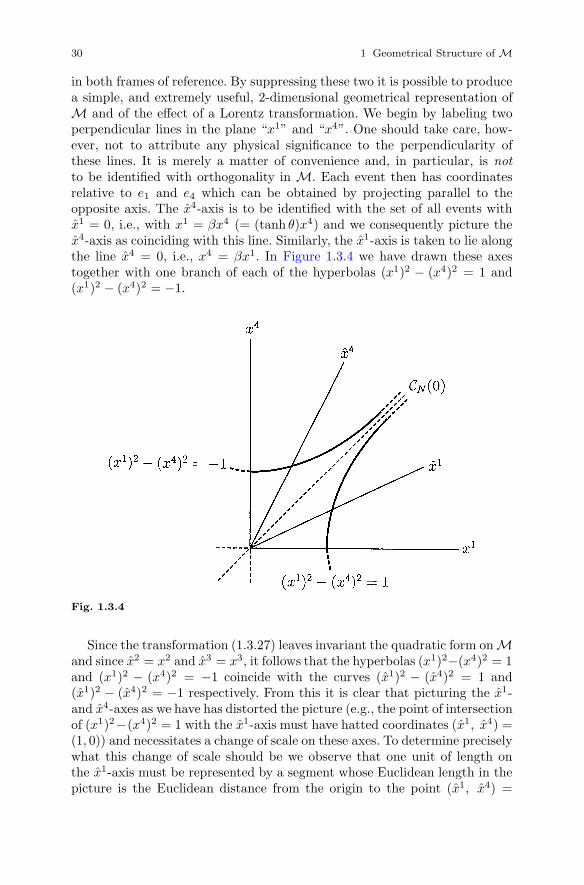
30 1 Geometrical Structure of M
in both frames of reference. By suppressing these two it is possible to producea simple, and extremely useful, 2-dimensional geometrical representation ofM and of the effect of a Lorentz transformation. We begin by labeling twoperpendicular lines in the plane “x1” and “x4”. One should take care, how-ever, not to attribute any physical significance to the perpendicularity ofthese lines. It is merely a matter of convenience and, in particular, is notto be identified with orthogonality in M. Each event then has coordinatesrelative to e1 and e4 which can be obtained by projecting parallel to theopposite axis. The x4-axis is to be identified with the set of all events withx1 = 0, i.e., with x1 = βx4 (= (tanh θ)x4) and we consequently picture thex4-axis as coinciding with this line. Similarly, the x1-axis is taken to lie alongthe line x4 = 0, i.e., x4 = βx1. In Figure 1.3.4 we have drawn these axestogether with one branch of each of the hyperbolas (x1)2 − (x4)2 = 1 and(x1)2 − (x4)2 = −1.
Fig. 1.3.4
Since the transformation (1.3.27) leaves invariant the quadratic form on Mand since x2 = x2 and x3 = x3, it follows that the hyperbolas (x1)2−(x4)2 = 1and (x1)2 − (x4)2 = −1 coincide with the curves (x1)2 − (x4)2 = 1 and(x1)2 − (x4)2 = −1 respectively. From this it is clear that picturing the x1-and x4-axes as we have has distorted the picture (e.g., the point of intersectionof (x1)2−(x4)2 = 1 with the x1-axis must have hatted coordinates (x1, x4) =(1, 0)) and necessitates a change of scale on these axes. To determine preciselywhat this change of scale should be we observe that one unit of length onthe x1-axis must be represented by a segment whose Euclidean length in thepicture is the Euclidean distance from the origin to the point (x1, x4) =

1.3 The Lorentz Group 31
(1, 0). This point has unhatted coordinates (x1, x4) = ((1 − β2)−12 ,
β(1 − β2)−12 ) (by (1.3.29)) and the Euclidean distance from this point to
the origin is, by the distance formula, (1 + β2)12 (1 − β2)−
12 . A similar ar-
gument shows that one unit of time on the x4-axis must also be representedby a segment of Euclidean length (1 + β2)
12 (1 − β2)−
12 . However, before we
can legitimately calibrate these axes with this unit we must verify that allof the hyperbolas (x1)2 − (x4)2 = ±k2 (k > 0) intersect the x1- and x4-axesa Euclidean distance k(1 + β2)
12 (1 − β2)−
12 from the origin (the calibration
must be consistent with the invariance of these hyperbolas under (1.3.27)).
Exercise 1.3.19 Verify this.
With this we have justified the calibration of the axes shown in Figure 1.3.5.
Fig. 1.3.5
Exercise 1.3.20 Show that with this calibration of the x1- and x4-axes thehatted coordinates of any event can be obtained geometrically by projectingparallel to the opposite axis.
From this it is clear that the dotted lines in Figure 1.3.5 parallel to the x1-and x4-axes and through the points (x1, x4) = (0, 1) and (x1, x4) = (1, 0)are the lines x4 = 1 and x1 = 1 respectively.
Exercise 1.3.21 Show that, for any k, the line x4 = k intersects the hyper-bola (x1)2 − (x4)2 = −k2 only at the point (x1, x4) = (0, k), where it is, infact, the tangent line. Similarly, x1 = k is tangent to (x1)2 − (x4)2 = k2 at(x1, x4) = (k, 0) and intersects this hyperbola only at that point.
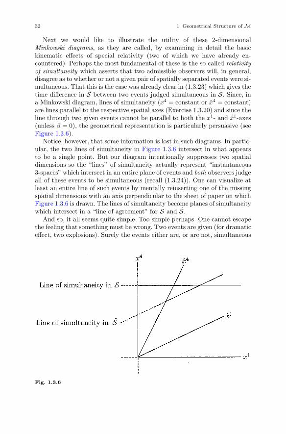
32 1 Geometrical Structure of M
Next we would like to illustrate the utility of these 2-dimensionalMinkowski diagrams, as they are called, by examining in detail the basickinematic effects of special relativity (two of which we have already en-countered). Perhaps the most fundamental of these is the so-called relativityof simultaneity which asserts that two admissible observers will, in general,disagree as to whether or not a given pair of spatially separated events were si-multaneous. That this is the case was already clear in (1.3.23) which gives thetime difference in S between two events judged simultaneous in S. Since, ina Minkowski diagram, lines of simultaneity (x4 = constant or x4 = constant)are lines parallel to the respective spatial axes (Exercise 1.3.20) and since theline through two given events cannot be parallel to both the x1- and x1-axes(unless β = 0), the geometrical representation is particularly persuasive (seeFigure 1.3.6).
Notice, however, that some information is lost in such diagrams. In partic-ular, the two lines of simultaneity in Figure 1.3.6 intersect in what appearsto be a single point. But our diagram intentionally suppresses two spatialdimensions so the “lines” of simultaneity actually represent “instantaneous3-spaces” which intersect in an entire plane of events and both observers judgeall of these events to be simultaneous (recall (1.3.24)). One can visualize atleast an entire line of such events by mentally reinserting one of the missingspatial dimensions with an axis perpendicular to the sheet of paper on whichFigure 1.3.6 is drawn. The lines of simultaneity become planes of simultaneitywhich intersect in a “line of agreement” for S and S.
And so, it all seems quite simple. Too simple perhaps. One cannot escapethe feeling that something must be wrong. Two events are given (for dramaticeffect, two explosions). Surely the events either are, or are not, simultaneous
Fig. 1.3.6
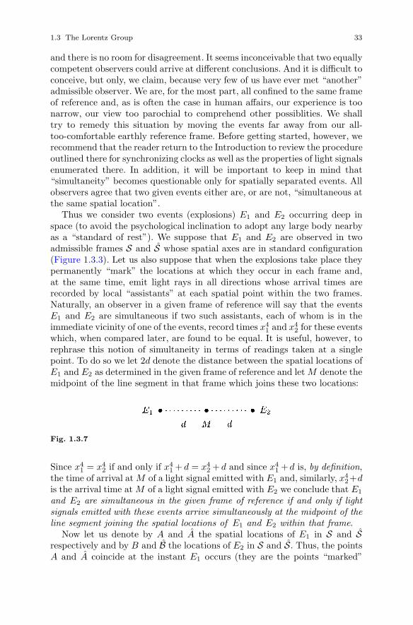
1.3 The Lorentz Group 33
and there is no room for disagreement. It seems inconceivable that two equallycompetent observers could arrive at different conclusions. And it is difficult toconceive, but only, we claim, because very few of us have ever met “another”admissible observer. We are, for the most part, all confined to the same frameof reference and, as is often the case in human affairs, our experience is toonarrow, our view too parochial to comprehend other possiblities. We shalltry to remedy this situation by moving the events far away from our all-too-comfortable earthly reference frame. Before getting started, however, werecommend that the reader return to the Introduction to review the procedureoutlined there for synchronizing clocks as well as the properties of light signalsenumerated there. In addition, it will be important to keep in mind that“simultaneity” becomes questionable only for spatially separated events. Allobservers agree that two given events either are, or are not, “simultaneous atthe same spatial location”.
Thus we consider two events (explosions) E1 and E2 occurring deep inspace (to avoid the psychological inclination to adopt any large body nearbyas a “standard of rest”). We suppose that E1 and E2 are observed in twoadmissible frames S and S whose spatial axes are in standard configuration(Figure 1.3.3). Let us also suppose that when the explosions take place theypermanently “mark” the locations at which they occur in each frame and,at the same time, emit light rays in all directions whose arrival times arerecorded by local “assistants” at each spatial point within the two frames.Naturally, an observer in a given frame of reference will say that the eventsE1 and E2 are simultaneous if two such assistants, each of whom is in theimmediate vicinity of one of the events, record times x4
1 and x42 for these events
which, when compared later, are found to be equal. It is useful, however, torephrase this notion of simultaneity in terms of readings taken at a singlepoint. To do so we let 2d denote the distance between the spatial locations ofE1 and E2 as determined in the given frame of reference and let M denote themidpoint of the line segment in that frame which joins these two locations:
Fig. 1.3.7
Since x41 = x4
2 if and only if x41 + d = x4
2 + d and since x41 + d is, by definition,
the time of arrival at M of a light signal emitted with E1 and, similarly, x42+d
is the arrival time at M of a light signal emitted with E2 we conclude that E1
and E2 are simultaneous in the given frame of reference if and only if lightsignals emitted with these events arrive simultaneously at the midpoint of theline segment joining the spatial locations of E1 and E2 within that frame.
Now let us denote by A and A the spatial locations of E1 in S and Srespectively and by B and B the locations of E2 in S and S. Thus, the pointsA and A coincide at the instant E1 occurs (they are the points “marked”
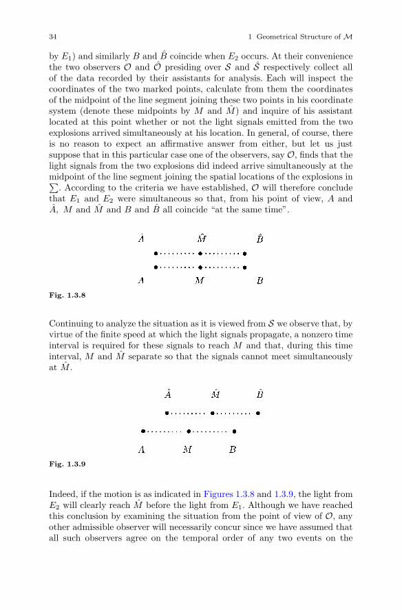
34 1 Geometrical Structure of M
by E1) and similarly B and B coincide when E2 occurs. At their conveniencethe two observers O and O presiding over S and S respectively collect allof the data recorded by their assistants for analysis. Each will inspect thecoordinates of the two marked points, calculate from them the coordinatesof the midpoint of the line segment joining these two points in his coordinatesystem (denote these midpoints by M and M) and inquire of his assistantlocated at this point whether or not the light signals emitted from the twoexplosions arrived simultaneously at his location. In general, of course, thereis no reason to expect an affirmative answer from either, but let us justsuppose that in this particular case one of the observers, say O, finds that thelight signals from the two explosions did indeed arrive simultaneously at themidpoint of the line segment joining the spatial locations of the explosions in∑
. According to the criteria we have established, O will therefore concludethat E1 and E2 were simultaneous so that, from his point of view, A andA, M and M and B and B all coincide “at the same time”.
Fig. 1.3.8
Continuing to analyze the situation as it is viewed from S we observe that, byvirtue of the finite speed at which the light signals propagate, a nonzero timeinterval is required for these signals to reach M and that, during this timeinterval, M and M separate so that the signals cannot meet simultaneouslyat M .
Fig. 1.3.9
Indeed, if the motion is as indicated in Figures 1.3.8 and 1.3.9, the light fromE2 will clearly reach M before the light from E1. Although we have reachedthis conclusion by examining the situation from the point of view of O, anyother admissible observer will necessarily concur since we have assumed thatall such observers agree on the temporal order of any two events on the
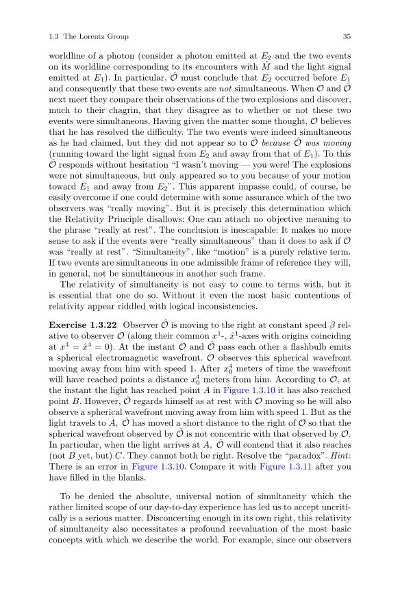
1.3 The Lorentz Group 35
worldline of a photon (consider a photon emitted at E2 and the two eventson its worldline corresponding to its encounters with M and the light signalemitted at E1). In particular, O must conclude that E2 occurred before E1
and consequently that these two events are not simultaneous. When O and Onext meet they compare their observations of the two explosions and discover,much to their chagrin, that they disagree as to whether or not these twoevents were simultaneous. Having given the matter some thought, O believesthat he has resolved the difficulty. The two events were indeed simultaneousas he had claimed, but they did not appear so to O because O was moving(running toward the light signal from E2 and away from that of E1). To thisO responds without hesitation “I wasn’t moving — you were! The explosionswere not simultaneous, but only appeared so to you because of your motiontoward E1 and away from E2”. This apparent impasse could, of course, beeasily overcome if one could determine with some assurance which of the twoobservers was “really moving”. But it is precisely this determination whichthe Relativity Principle disallows: One can attach no objective meaning tothe phrase “really at rest”. The conclusion is inescapable: It makes no moresense to ask if the events were “really simultaneous” than it does to ask if Owas “really at rest”. “Simultaneity”, like “motion” is a purely relative term.If two events are simultaneous in one admissible frame of reference they will,in general, not be simultaneous in another such frame.
The relativity of simultaneity is not easy to come to terms with, but itis essential that one do so. Without it even the most basic contentions ofrelativity appear riddled with logical inconsistencies.
Exercise 1.3.22 Observer O is moving to the right at constant speed β rel-ative to observer O (along their common x1-, x1-axes with origins coincidingat x4 = x4 = 0). At the instant O and O pass each other a flashbulb emitsa spherical electromagnetic wavefront. O observes this spherical wavefrontmoving away from him with speed 1. After x4
0 meters of time the wavefrontwill have reached points a distance x4
0 meters from him. According to O, atthe instant the light has reached point A in Figure 1.3.10 it has also reachedpoint B. However, O regards himself as at rest with O moving so he will alsoobserve a spherical wavefront moving away from him with speed 1. But as thelight travels to A, O has moved a short distance to the right of O so that thespherical wavefront observed by O is not concentric with that observed by O.In particular, when the light arrives at A, O will contend that it also reaches(not B yet, but) C. They cannot both be right. Resolve the “paradox”. Hint :There is an error in Figure 1.3.10. Compare it with Figure 1.3.11 after youhave filled in the blanks.
To be denied the absolute, universal notion of simultaneity which therather limited scope of our day-to-day experience has led us to accept uncriti-cally is a serious matter. Disconcerting enough in its own right, this relativityof simultaneity also necessitates a profound reevaluation of the most basicconcepts with which we describe the world. For example, since our observers

36 1 Geometrical Structure of M
Fig. 1.3.10
O and O need not agree on the time lapse between two events even when oneof them measures it to be zero, one could scarcely expect them to agree onthe elapsed time between two arbitrarily given events. And, indeed, we havealready seen in (1.3.20) that Δx4 and Δx4 are generally not equal. This effect,known as time dilation, has a particularly nice geometrical representation ina Minkowski diagram (see Figure 1.3.12). E1 (resp., E2) can be identifiedphysically with the appearance of the reading “1” on the clock at the originof S (resp., S). In S, E1 is simultaneous with E3 which corresponds to areading strictly less than 1 on the clock at the origin in S. Since the clocksat the origins of S and S agreed at x4 = x4 = 0, O concludes that O’sclock is running slow. Indeed, (1.3.21) and (1.3.22) show that each observesthe other’s time dilated by the same constant factor γ = (1 − β2)−
12 . The
moral of the story, perhaps a bit too tersely stated, is that “moving clocksrun slow”.
Exercise 1.3.23 Pions are subatomic particles which decay spontaneouslyand have a half-life (at rest) of 1.8 × 10⁻⁸ sec (= 5.4m). A beam of pionsis accelerated to a speed of β = 0.99. One would expect that the beamwould drop to one-half its original intensity after travelling a distance of(0.99)(5.4m) = 5.3m. However, it is found experimentally that the beamreaches one-half intensity after travelling approximately 38m. Explain! Hint :Let S denote the laboratory frame of reference, S the rest frame of the pi-ons and assume that S and S are related by (1.3.27) and (1.3.29). Draw aMinkowski diagram which represents the situation.
Return for a moment to Figure 1.3.12 and, in particular, to the line x4 = 1.Each point on this line can be identified with the appearance of the reading“1” on a clock that is stationary at some point in
∑. These all occur “simul-
taneously” for O because his clocks have been synchronized. However, eachof these events occurs at a different “time” in S so O will disagree. Clocks atdifferent locations in
∑read 1 at different “times” so, according to O, they
cannot be synchronized.Here is an old, and much abused, “paradox” with its roots in the phe-
nomenon of time dilation, or rather, in a basic misunderstanding of thatphenomenon. Suppose that, at (0, 0, 0, 0), two identical twins part company.
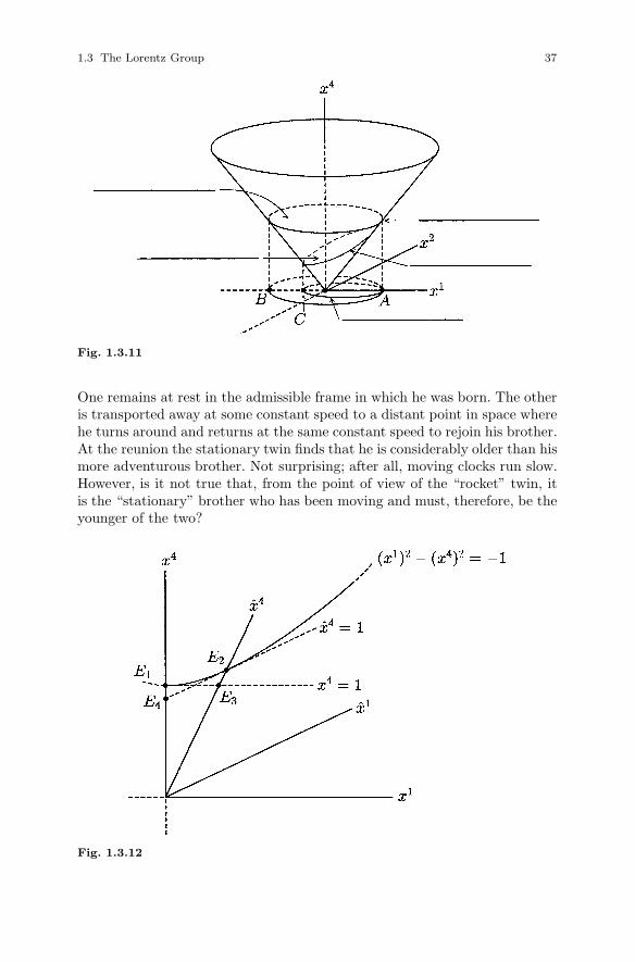
1.3 The Lorentz Group 37
Fig. 1.3.11
One remains at rest in the admissible frame in which he was born. The otheris transported away at some constant speed to a distant point in space wherehe turns around and returns at the same constant speed to rejoin his brother.At the reunion the stationary twin finds that he is considerably older than hismore adventurous brother. Not surprising; after all, moving clocks run slow.However, is it not true that, from the point of view of the “rocket” twin, itis the “stationary” brother who has been moving and must, therefore, be theyounger of the two?
Fig. 1.3.12

38 1 Geometrical Structure of M
The error concealed in this argument, of course, is that it hinges upon asupposed symmetry between the two twins which simply does not exist. Ifthe stationary twin does, in fact, remain at rest in an admissible frame, thenhis brother certainly does not. Indeed, to turn around and return midwaythrough his journey he must “transfer” from one admissible frame to anotherand, in practice, such a transfer would require accelerations (slow down, turnaround, speed up) and these accelerations would be experienced only by thetraveller and not by his brother. Nothing we have done thus far equips usto deal with these accelerations and so we can come to no conclusions abouttheir physical effects (we will pursue this further in Section 1.4). That theydo have physical effects, however, can be surmised even now by idealizing thesituation a bit. Let us replace our two twins with three admissible frames: S(stationary twin), S (rocket twin on his outward journey) and ˆS (rocket twinon his return journey). What this amounts to is the assumption that the twoindividuals involved compare ages in passing (without stopping to discuss it)at the beginning and end of the trip and that, at the turnaround point, thetraveller “jumps” instantaneously from one admissible frame to another (hecannot do that, of course, but it seems reasonable that, with a sufficientlydurable observer, we could approximate such a jump arbitrarily well by a“large” acceleration over a “small” time interval). Figure 1.3.13 representsthe outward journey from O to the turnaround event T .
Fig. 1.3.13
Notice that, in S, T is simultaneous with the event P on the worldlineof the stay-at-home. In S, P is simultaneous with some earlier event on theworldline of the traveller. Each sees the other’s time dilated. Figure 1.3.14represents the return journey. Notice that, in ˆS, T is simultaneous with (notP , but) the event Q on the worldline of the stationary twin, whereas, in S, Qis simultaneous with some later event on the traveller’s worldline. Each seesthe other’s time dilated. Now, put the two pictures together in Figure 1.3.15

1.3 The Lorentz Group 39
Fig. 1.3.14
and notice that in “jumping” from S to ˆS, our rocket twin has also jumpedover the entire interval from P to Q on the worldline of his brother; an intervalover which his brother ages, but he does not. The lesson to be learned is that,while all motion is indeed relative, it is not all physically equivalent.
Exercise 1.3.24 Account, in a sentence or two, for the “missing” time in
Figure 1.3.15. Hint :2β
1 + β2> β for 0 < β < 1.
There is one last kinematic consequence of the relativity of simultaneity,as interesting, as important and as surprising as time dilation. To trace itsorigins we return once again to the explosions E1 and E2, observed by S andS and discussed on pages 33–36. Recall that the points A in
∑and A in
∑coincided when E1 occurred, whereas B in
∑and B in
∑coincided when E2
occurred. Since the two events were simultaneous in S, the observer O willconclude that A coincides with A at the same instant that B coincides withB and, in particular, that the segments AB and AB have the same length(see Figure 1.3.8). However, in S, E2 occurred before E1 so B coincideswith B before A coincides with A and O must conclude that the lengthof AB is greater than the length of AB. More generally, two objects (say,measuring rods) in relative motion are considered to be equal in length if,when they pass each other, their respective endpoints A, A and B, B coincidesimultaneously. But, “simultaneously” according to whom? Here we have twoevents (the coincidence of A and A and the coincidence of B and B) and wehave seen that if one admissible observer claims that they are simultaneous(i.e., that the lengths AB and AB are equal), then another will, in general,disagree and we have no reason to prefer the judgment of one such observer tothat of another (Relativity Principle). “Length”, we must conclude, cannotbe regarded as an objective attribute of the rods, but is rather simply theresult of a specific measurement which we can no longer go on believingmust be the same for all observers. Notice also that these conclusions have
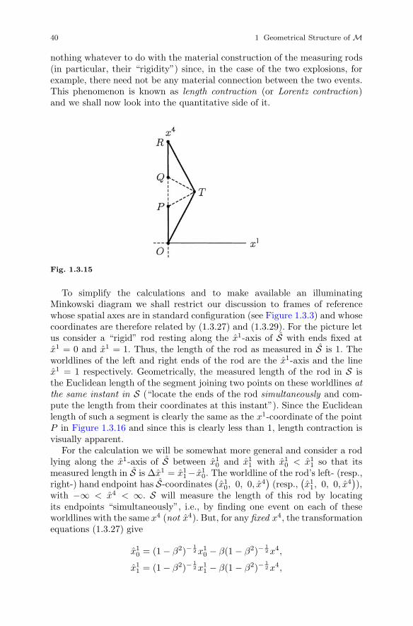
40 1 Geometrical Structure of M
nothing whatever to do with the material construction of the measuring rods(in particular, their “rigidity”) since, in the case of the two explosions, forexample, there need not be any material connection between the two events.This phenomenon is known as length contraction (or Lorentz contraction)and we shall now look into the quantitative side of it.
Fig. 1.3.15
To simplify the calculations and to make available an illuminatingMinkowski diagram we shall restrict our discussion to frames of referencewhose spatial axes are in standard configuration (see Figure 1.3.3) and whosecoordinates are therefore related by (1.3.27) and (1.3.29). For the picture letus consider a “rigid” rod resting along the x1-axis of S with ends fixed atx1 = 0 and x1 = 1. Thus, the length of the rod as measured in S is 1. Theworldlines of the left and right ends of the rod are the x1-axis and the linex1 = 1 respectively. Geometrically, the measured length of the rod in S isthe Euclidean length of the segment joining two points on these worldlines atthe same instant in S (“locate the ends of the rod simultaneously and com-pute the length from their coordinates at this instant”). Since the Euclideanlength of such a segment is clearly the same as the x1-coordinate of the pointP in Figure 1.3.16 and since this is clearly less than 1, length contraction isvisually apparent.
For the calculation we will be somewhat more general and consider a rodlying along the x1-axis of S between x1
0 and x11 with x1
0 < x11 so that its
measured length in S is Δx1 = x11− x1
0. The worldline of the rod’s left- (resp.,right-) hand endpoint has S-coordinates
(x1
0, 0, 0, x4)
(resp.,(x1
1, 0, 0, x4)),
with −∞ < x4 < ∞. S will measure the length of this rod by locatingits endpoints “simultaneously”, i.e., by finding one event on each of theseworldlines with the same x4 (not x4). But, for any fixed x4, the transformationequations (1.3.27) give
x10 = (1 − β2)−
12 x1
0 − β(1 − β2)−12 x4,
x11 = (1 − β2)−
12 x1
1 − β(1 − β2)−12 x4,

1.3 The Lorentz Group 41
Fig. 1.3.16
so that Δx1 = (1 − β2)−12 Δx1 and therefore
Δx1 = (1 − β2)12 Δx1. (1.3.36)
Since (1 − β2)12 < 1 we find that the measured length of the rod in S is less
than its measured length in S by a factor of√
1 − β2. By reversing the rolesof S and S we again find that this effect is entirely symmetrical.
Exercise 1.3.25 Return to Exercise 1.3.23 and offer another explanationbased, not on time dilation, but on length contraction.
As it is with time dilation, the correct physical interpretation of theLorentz contraction often requires rather subtle and delicate argument.
Exercise 1.3.26 Imagine a barn which, at rest, measures 8 meters in length.A (very fast) runner carries a pole of rest length 16 meters toward the barnat such a high speed that, for an observer at rest with the barn, it appearsLorentz contracted to 8 meters and therefore fits inside the barn. This ob-server slams the front door shut at the instant the back of the pole entersthe front of the barn and so encloses the pole entirely within the barn. Butis it not true that the runner sees the barn Lorentz contracted to 4 metersso that the 16 meter pole could never fit entirely within it? Resolve the diffi-culty! Hint : Let S and S respectively denote the rest frames of the barn andthe pole and assume that these frames are related by (1.3.27) and (1.3.29).Calculate β. Suppose the front of the pole enters the front of the barn at(0, 0, 0, 0). Now consider the two events at which the front of the pole hitsthe back of the barn and the back of the pole enters the front of the barn.

42 1 Geometrical Structure of M
Finally, think about the maximum speed at which the signal to stop can becommunicated from the front to the back of the pole.
The underlying message of Exercise 1.3.26 would seem to be that theclassical notion of a perfectly “rigid” body has no place in relativity, even asan idealization. The pole must compress since otherwise the signal to haltwould proceed from the front to the back instantaneously and, in particular,the situation described in the exercise would, indeed, be “paradoxical”, i.e.,represent a logical inconsistency.
1.4 Timelike Vectors and Curves
Let us now consider in somewhat more detail a pair of events x0 and x forwhich x− x0 is timelike, i.e., Q(x− x0) < 0. Relative to any admissible basis{ea} we have (Δx1)2 + (Δx2)2 + (Δx3)2 < (Δx4)2. Clearly then, Δx4 �= 0and we may assume without loss of generality that Δx4 > 0, i.e., that x− x0
is future-directed. Thus, we obtain
((Δx1)2 + (Δx2)2 + (Δx3)2)12
Δx4< 1.
Physically, it is therefore clear that if one were to move with speed
((Δx1)2 + (Δx2)2 + (Δx3)2)12
Δx4
relative to the frame S corresponding to {ea} along the line in∑
from(x1
0, x20, x3
0
)to (x1, x2, x3) and if one were present at x0, then one would also
experience x, i.e., that there is an admissible frame of reference S in whichx0 and x occur at the same spatial point, one after the other. Specifically, wenow prove that if one chooses β = ((Δx1)2 + (Δx2)2 + (Δx3)2)1/2/Δx4 andlets d1, d2 and d3 be the direction cosines in
∑of the directed line segment
from(x1
0, x20, x3
0
)to (x1, x2, x3), then the basis {ea} for M obtained from
{ea} by performing any Lorentz transformation whose fourth row is Λ4i =
−β(1−β2)−1/2 di, i = 1, 2, 3, and Λ44 = (1−β2)−1/2 = γ, has the property
that Δx1 = Δx2 = Δx3 = 0.
Exercise 1.4.1 There will, in general, be many Lorentz transformationswith this fourth row. Show that defining the remaining entries by Λi
4 =−βγdi, i = 1, 2, 3, and Λi
j = (γ − 1)didj + δij , i, j = 1, 2, 3 (δi
j being theKronecker delta) gives an element of L.
To prove this we compute Δx4 = Λ4bΔxb. To simplify the calculations we
let Δ⇀x = ((Δx1)2+(Δx2)2+(Δx3)2)1/2. We may clearly assume that Δ
⇀x �= 0
since otherwise there is nothing to prove. Thus, β2 = Δ⇀x2/(Δx4)2, γ =
Δx4/√−Q(x − x0), βγ = Δ
⇀x/√−Q(x − x0) and di = Δxi/Δ
⇀x for i =
1, 2, 3. From (1.3.20) we therefore obtain
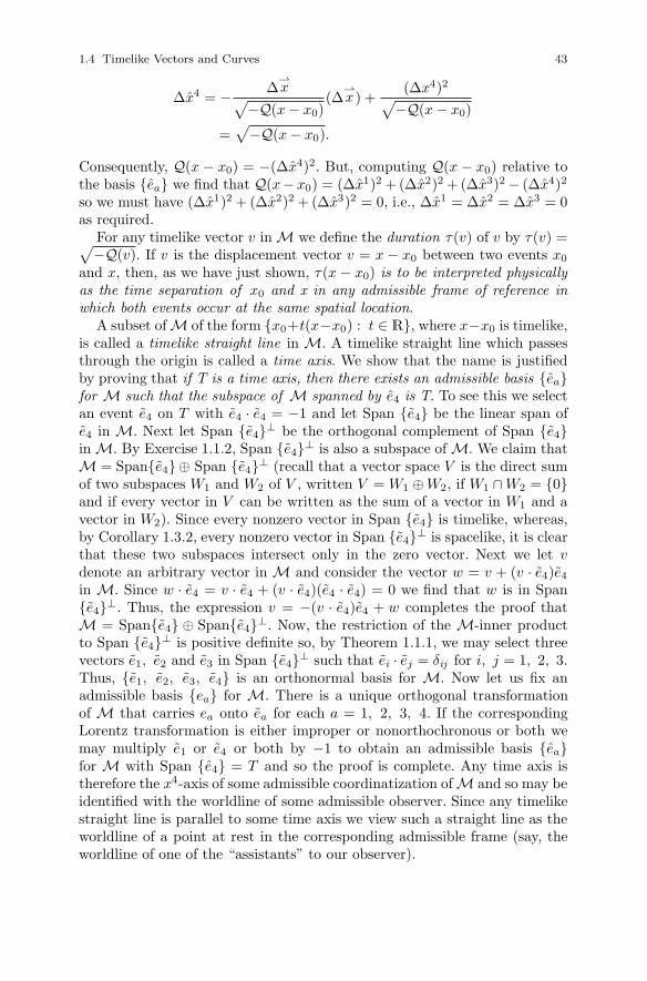
1.4 Timelike Vectors and Curves 43
Δx4 = − Δ⇀x√
−Q(x − x0)(Δ
⇀x) +
(Δx4)2√−Q(x − x0)
=√−Q(x − x0).
Consequently, Q(x − x0) = −(Δx4)2. But, computing Q(x − x0) relative tothe basis {ea} we find that Q(x− x0) = (Δx1)2 + (Δx2)2 + (Δx3)2 − (Δx4)2
so we must have (Δx1)2 + (Δx2)2 + (Δx3)2 = 0, i.e., Δx1 = Δx2 = Δx3 = 0as required.
For any timelike vector v in M we define the duration τ(v) of v by τ(v) =√−Q(v). If v is the displacement vector v = x − x0 between two events x0
and x, then, as we have just shown, τ(x − x0) is to be interpreted physicallyas the time separation of x0 and x in any admissible frame of reference inwhich both events occur at the same spatial location.
A subset of M of the form {x0+t(x−x0) : t ∈ R}, where x−x0 is timelike,is called a timelike straight line in M. A timelike straight line which passesthrough the origin is called a time axis. We show that the name is justifiedby proving that if T is a time axis, then there exists an admissible basis {ea}for M such that the subspace of M spanned by e4 is T. To see this we selectan event e4 on T with e4 · e4 = −1 and let Span {e4} be the linear span ofe4 in M. Next let Span {e4}⊥ be the orthogonal complement of Span {e4}in M. By Exercise 1.1.2, Span {e4}⊥ is also a subspace of M. We claim thatM = Span{e4}⊕ Span {e4}⊥ (recall that a vector space V is the direct sumof two subspaces W1 and W2 of V , written V = W1 ⊕W2, if W1 ∩W2 = {0}and if every vector in V can be written as the sum of a vector in W1 and avector in W2). Since every nonzero vector in Span {e4} is timelike, whereas,by Corollary 1.3.2, every nonzero vector in Span {e4}⊥ is spacelike, it is clearthat these two subspaces intersect only in the zero vector. Next we let vdenote an arbitrary vector in M and consider the vector w = v + (v · e4)e4
in M. Since w · e4 = v · e4 + (v · e4)(e4 · e4) = 0 we find that w is in Span{e4}⊥. Thus, the expression v = −(v · e4)e4 + w completes the proof thatM = Span{e4} ⊕ Span{e4}⊥. Now, the restriction of the M-inner productto Span {e4}⊥ is positive definite so, by Theorem 1.1.1, we may select threevectors e1, e2 and e3 in Span {e4}⊥ such that ei · ej = δij for i, j = 1, 2, 3.Thus, {e1, e2, e3, e4} is an orthonormal basis for M. Now let us fix anadmissible basis {ea} for M. There is a unique orthogonal transformationof M that carries ea onto ea for each a = 1, 2, 3, 4. If the correspondingLorentz transformation is either improper or nonorthochronous or both wemay multiply e1 or e4 or both by −1 to obtain an admissible basis {ea}for M with Span {e4} = T and so the proof is complete. Any time axis istherefore the x4-axis of some admissible coordinatization of M and so may beidentified with the worldline of some admissible observer. Since any timelikestraight line is parallel to some time axis we view such a straight line as theworldline of a point at rest in the corresponding admissible frame (say, theworldline of one of the “assistants” to our observer).
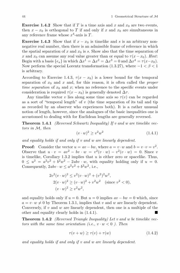
44 1 Geometrical Structure of M
Exercise 1.4.2 Show that if T is a time axis and x and x0 are two events,then x − x0 is orthogonal to T if and only if x and x0 are simultaneous inany reference frame whose x4-axis is T .
Exercise 1.4.3 Show that if x − x0 is timelike and s is an arbitrary non-negative real number, then there is an admissible frame of reference in whichthe spatial separation of x and x0 is s. Show also that the time separation ofx and x0 can assume any real value greater than or equal to τ(x− x0). Hint :Begin with a basis {ea} in which Δx1 = Δx2 = Δx3 = 0 and Δx4 = τ(x−x0).Now perform the special Lorentz transformation (1.3.27), where −1 < β < 1is arbitrary.
According to Exercise 1.4.3, τ(x − x0) is a lower bound for the temporalseparation of x0 and x and, for this reason, it is often called the propertime separation of x0 and x; when no reference to the specific events underconsideration is required τ(x − x0) is generally denoted Δτ .
Any timelike vector v lies along some time axis so τ(v) can be regardedas a sort of “temporal length” of v (the time separation of its tail and tipas recorded by an observer who experiences both). It is a rather unusualnotion of length, however, since the analogues of the basic inequalities one isaccustomed to dealing with for Euclidean lengths are generally reversed.
Theorem 1.4.1 (Reversed Schwartz Inequality) If v and w are timelike vec-tors in M, then
(v · w)2 ≥ v2w2 (1.4.1)
and equality holds if and only if v and w are linearly dependent.
Proof: Consider the vector u = av − bw , where a = v ·w and b = v ·v = v2.Observe that u · v = av 2 − bv · w = v2(v · w) − v2(v · w) = 0. Since vis timelike, Corollary 1.3.2 implies that u is either zero or spacelike. Thus,0 ≤ u2 = a2v2 + b2w2 − 2abv · w, with equality holding only if u = 0.Consequently, 2abv · w ≤ a2v2 + b2w2, i.e.,
2v2(v · w)2 ≤ v2(v · w)2 + (v2)2w2,
2(v · w)2 ≥ (v · w)2 + v2w2 (since v2 < 0),
(v · w)2 ≥ v2w2,
and equality holds only if u = 0. But u = 0 implies av − bw = 0 which, sincea = v ·w �= 0 by Theorem 1.3.1, implies that v and w are linearly dependent.Conversely, if v and w are linearly dependent, then one is a multiple of theother and equality clearly holds in (1.4.1). �Theorem 1.4.2 (Reversed Triangle Inequality) Let v and w be timelike vec-tors with the same time orientation (i.e., v · w < 0 ). Then
τ(v + w) ≥ τ(v) + τ(w) (1.4.2)
and equality holds if and only if v and w are linearly dependent.

1.4 Timelike Vectors and Curves 45
Proof: By Theorem 1.4.1, (v · w)2 ≥ v2w2 = (−v2)(−w2) so |v · w| ≥√−v2
√−w2. But (v · w) < 0 so we must have v · w ≤ −
√−v2
√−w2 and
therefore− 2v · w ≥ 2
√−v2√−w2. (1.4.3)
Now, by Exercise 1.3.2, v + w is timelike. Moreover, −(v + w)2 = −v2 − 2v ·w − w2 ≥ −v2 + 2
√−v2
√−w2 − w2 by (1.4.3). Thus,
−(v + w)2 ≥(√
−v2 +√−w2)2
,√−(v + w)2 ≥
√−v2 +
√−w2,√
−Q(v + w) ≥√−Q(v) +
√−Q(w),
τ(v + w) ≥ τ(v) + τ(w),
as required. If equality holds in (1.4.2), then, by reversing the preceding steps,we obtain
−2v · w = 2√
v2√
−w2
and therefore (v · w)2 = v2w2 so, by Theorem 1.4.1, v and w are linearlydependent. �
To extend Theorem 1.4.2 to arbitrary finite sums of similarly orientedtimelike vectors (and for other purposes as well) we require:
Lemma 1.4.3 The sum of any finite number of vectors in M all of whichare timelike or null and all future-directed (resp., past-directed) is timelikeand future-directed (resp., past-directed) except when all of the vectors arenull and parallel, in which case the sum is null and future-directed (resp.,past-directed).
Proof: It suffices to prove the result for future-directed vectors since thecorresponding result for past-directed vectors will then follow by changingsigns. Moreover, it is clear that any sum of future-directed vectors is, indeed,future-directed.
First we observe that if v1 and v2 are timelike and future-directed, thenv1 · v1 < 0, v2 · v2 < 0 and v1 · v2 < 0 so (v1 + v2) · (v1 + v2) = v1 · v1 + 2v1 ·v2 + v2 · v2 < 0 and therefore v1 + v2 is timelike.
Exercise 1.4.4 Show that if v1 is timelike, v2 is null and both are future-directed, then v1 + v2 is timelike and future-directed.
Next suppose that v1 and v2 are null and future-directed. We show that v1+v2
is timelike unless v1 and v2 are parallel (in which case, it is obviously null).To this end we note that (v1 + v2) · (v1 + v2) = 2v1 · v2. By Theorem 1.2.1,v1 · v2 = 0 if and only if v1 and v2 are parallel. Suppose then that v1 andv2 are not parallel. Fix an admissible basis {ea} for M and let v1 = va
1ea
and v2 = va2ea. For each n = 1, 2, 3, . . . , define wn in M by wn = v1
1e1 +v21e2 + v3
1e3 +(v41 + 1
n
)e4. Then each wn is timelike and future-directed.

46 1 Geometrical Structure of M
By Theorem 1.3.1, 0 > wn · v2 = v1 · v2 − 1nv42 , i.e., v1 · v2 < 1
nv42 for every n.
Thus, v1 · v2 ≤ 0. But v1 · v2 �= 0 by assumption so v1 · v2 < 0 and therefore(v1 + v2) · (v1 + v2) < 0 as required.
Exercise 1.4.5 Complete the proof by induction. �
Corollary 1.4.4 Let v1, . . . , vn be timelike vectors, all with the same timeorientation. Then
τ(v1 + v2 + · · · + vn) ≥ τ(v1) + τ(v2) + · · · + τ(vn) (1.4.4)
and equality holds if and only if v1, v2, . . . , vn are all parallel.
Proof: Inequality (1.4.4) is clear from Theorem 1.4.2 and Lemma 1.4.3. Weshow, by induction on n, that equality in (1.4.4) implies that v1, . . . , vn areall parallel. For n = 2 this is just Theorem 1.4.2. Thus, we assume that thestatement is true for sets of n vectors and consider a set v1, . . . , vn, vn+1 oftimelike vectors which are, say, future-directed and for which
τ(v1 + · · · + vn + vn+1) = τ(v1) + · · · + τ(vn) + τ(vn+1).
v1 + · · · + vn is timelike and future-directed so, again by Theorem 1.4.2,
τ(v1 + · · · + vn) + τ(vn+1) ≤ τ(v1) + · · · + τ(vn) + τ(vn+1).
We claim that, in fact, equality must hold here. Indeed, otherwise we haveτ(v1 + · · · + vn) < τ(v1) + · · · + τ(vn) and so (Theorem 1.4.2 again) τ(v1 +· · · + vn−1) < τ(v1) + · · · + τ(vn−1). Continuing the process we eventuallyconclude that τ(v1) < τ(v1) which is a contradiction. Thus,
τ(v1 + · · · + vn) = τ(v1) + · · · + τ(vn)
and the induction hypothesis implies that v1, . . . , vn are all parallel. Letv = v1 + · · ·+vn. Then v is timelike and future-directed. Thus, τ(v+vn+1) =τ(v)+τ(vn+1) and one more application of Theorem 1.4.2 implies that vn+1 isparallel to v and therefore to all of v1, . . . , vn and the proof is complete. �
Corollary 1.4.5 Let v and w be two nonparallel null vectors. Then v and whave the same time orientation if and only if v · w < 0.
Proof: Suppose first that v and w have the same time orientation. ByLemma 1.4.3, v + w is timelike so 0 > (v + w) · (v + w) = 2v ·w so v ·w < 0.Conversely, if v and w have opposite time orientation, then v and −w havethe same time orientation so v · (−w) < 0 and therefore v · w > 0. �
The reason that the sense of the inequality in Theorem 1.4.2 is “reversed”becomes particularly transparent by choosing a coordinate system relative towhich v = (v1, v2, v3, v4), w = (w1, w2, w3, w4) and v+w = (0, 0, 0, v4+w4)(this simply amounts to taking the time axis through v + w as the x4-axis).For then τ(v) = ((v4)2 − (v1)2 − (v2)2 − (v3)2)
12 < v4 and τ(w) < w4, but
τ(v + w) = v4 + w4.
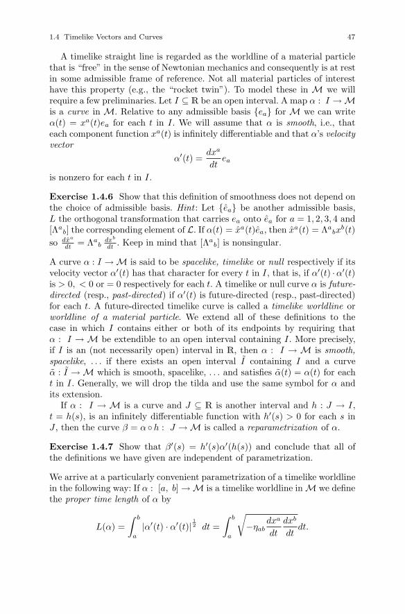
1.4 Timelike Vectors and Curves 47
A timelike straight line is regarded as the worldline of a material particlethat is “free” in the sense of Newtonian mechanics and consequently is at restin some admissible frame of reference. Not all material particles of interesthave this property (e.g., the “rocket twin”). To model these in M we willrequire a few preliminaries. Let I ⊆ R be an open interval. A map α : I → Mis a curve in M. Relative to any admissible basis {ea} for M we can writeα(t) = xa(t)ea for each t in I. We will assume that α is smooth, i.e., thateach component function xa(t) is infinitely differentiable and that α’s velocityvector
α′(t) =dxa
dtea
is nonzero for each t in I.
Exercise 1.4.6 Show that this definition of smoothness does not depend onthe choice of admissible basis. Hint : Let {ea} be another admissible basis,L the orthogonal transformation that carries ea onto ea for a = 1, 2, 3, 4 and[Λa
b] the corresponding element of L. If α(t) = xa(t)ea, then xa(t) = Λabx
b(t)so dxa
dt= Λa
bdxb
dt. Keep in mind that [Λa
b] is nonsingular.
A curve α : I → M is said to be spacelike, timelike or null respectively if itsvelocity vector α′(t) has that character for every t in I, that is, if α′(t) ·α′(t)is > 0, < 0 or = 0 respectively for each t. A timelike or null curve α is future-directed (resp., past-directed) if α′(t) is future-directed (resp., past-directed)for each t. A future-directed timelike curve is called a timelike worldline orworldline of a material particle. We extend all of these definitions to thecase in which I contains either or both of its endpoints by requiring thatα : I → M be extendible to an open interval containing I. More precisely,if I is an (not necessarily open) interval in R, then α : I → M is smooth,spacelike, . . . if there exists an open interval I containing I and a curveα : I → M which is smooth, spacelike, . . . and satisfies α(t) = α(t) for eacht in I. Generally, we will drop the tilda and use the same symbol for α andits extension.
If α : I → M is a curve and J ⊆ R is another interval and h : J → I,t = h(s), is an infinitely differentiable function with h′(s) > 0 for each s inJ , then the curve β = α ◦h : J → M is called a reparametrization of α.
Exercise 1.4.7 Show that β′(s) = h′(s)α′(h(s)) and conclude that all ofthe definitions we have given are independent of parametrization.
We arrive at a particularly convenient parametrization of a timelike worldlinein the following way: If α : [a, b] → M is a timelike worldline in M we definethe proper time length of α by
L(α) =∫ b
a
|α′(t) · α′(t)|12 dt =
∫ b
a
√−ηab
dxa
dt
dxb
dtdt.

48 1 Geometrical Structure of M
Exercise 1.4.8 Show that the definition of L(α) is independent ofparametrization.
As the appropriate physical interpretation of L(α) we take
The Clock Hypothesis: If α : [a, b] → M is a timelike worldline in M,then L(α) is interpreted as the time lapse between the events α(a) and α(b)as measured by an ideal standard clock carried along by the particle whoseworldline is represented by α.
The motivation for the Clock Hypothesis is at the same time “obvious” andsubtle. For it we shall require the following theorem which asserts that twoevents can be experienced by a single admissible observer if and only if some(not necessarily free) material particle has both on its worldline.
Theorem 1.4.6 Let p and q be two points in M. Then p− q is timelike andfuture-directed if and only if there exists a smooth, future-directed timelikecurve α : [a, b] → M such that α(a) = q and α(b) = p.
We postpone the proof for a moment to show its relevance to the ClockHypothesis. We partition the interval [a, b] into subintervals by a = t0 <t1 < . . . < tn−1 < tn = b. Then, by Theorem 1.4.6, each of the displace-ment vectors vi = α(ti) − α(ti−1) is timelike and future-directed. τ(vi) isthen interpreted as the time lapse between α(ti−1) and α(ti) as measured byan admissible observer who is present at both events. If the “material parti-cle” whose worldline is represented by α has constant velocity between theevents α(ti−1) and α(ti), then τ(vi) would be the time lapse between theseevents as measured by a clock carried along by the particle. Relative to anyadmissible frame,
τ(vi) =√−ηabΔxa
i Δxbi =
√−ηab
Δxai
Δti
Δxbi
ΔtiΔti.
By choosing Δti sufficiently small, Δx4i can be made small (by continuity
of α) and, since the speed of the particle relative to our frame of referenceis “nearly” constant over “small” x4-time intervals, τ(vi) should be a goodapproximation to the time lapse between α(ti−1) and α(ti) measured by thematerial particle. Consequently, the sum
n∑i=1
√−ηab
Δxai
Δti
Δxbi
ΔtiΔti (1.4.5)
approximates the time lapse between α(a) and α(b) that this particle mea-sures. The approximations become better as the Δti approach 0 and, in thelimit, the sum (1.4.5) approaches the definition of L(α).
The argument seems persuasive enough, but it clearly rests on an assump-tion about the behavior of ideal clocks that we had not previously madeexplicit, namely, that acceleration as such has no effect on their rates, i.e.,

1.4 Timelike Vectors and Curves 49
that the “instantaneous rate” of such a clock depends only on its instanta-neous speed and not on the rate at which this speed is changing. Justifyingsuch an assumption is a nontrivial matter. One must perform experimentswith various types of clocks subjected to real accelerations and, in the end,will no doubt be forced to a more modest proposal (“The Clock Hypothesis isvalid for such and such a clock over such and such a range of accelerations”).
For the proof of Theorem 1.4.6 we will require the following preliminaryresult.
Lemma 1.4.7 Let α : (A, B) → M be smooth, timelike and future-directedand fix a t0 in (A, B). Then there exists an ε > 0 such that (t0 − ε, t0 + ε)is contained in (A, B), α(t) is in the past time cone at α(t0) for every tin (t0 − ε, t0) and α(t) is in the future time cone at α(t0) for every t in(t0, t0 + ε).
Proof: We prove that there exists an ε1 > 0 such that α(t) is in C+T (α(t0))
for each t in (t0, t0 + ε1). The argument to produce an ε2 > 0 with α(t) inC−
T (α(t0)) for each t in (t0 − ε2, t0) is similar. Taking ε to be the smaller ofε1 and ε2 proves the lemma.
Fix an admissible basis {ea} and write α(t) = xa(t)ea for A < t < B.Now suppose that no such ε1 exists. Then one can produce a sequence t1 >t2 > · · · > t0 in (t0, B) such that limn→∞ tn = t0 and such that one of thefollowing is true:
(I) Q(α(tn) − α(t0)) ≥ 0 for all n (i.e., α(tn) − α(t0) is spacelike or null forevery n), or
(II) Q(α(tn)−α(t0)) < 0, but α(tn)−α(t0) is past-directed for every n (i.e.,α(tn) is in C−
T (α(t0)) for every n).
We show first that (I) is impossible. Suppose to the contrary that such asequence does exist. Then
Q(
α(tn) − α(t0)tn − t0
)≥ 0
for all n so
Q(
x1(tn) − x1(t0)tn − t0
, . . . ,x4(tn) − x4(t0)
tn − t0
)≥ 0.
Thus,
limn→∞Q
(x1(tn) − x1(t0)
tn − t0, . . . ,
x4(tn) − x4(t0)tn − t0
)≥ 0,
Q(
limn→∞
x1(tn) − x1(t0)tn − t0
, . . . , limn→∞
x4(tn) − x4(t0)tn − t0
)≥ 0,
Q(
dx1
dt(t0), . . . ,
dx4
dt(t0))
≥ 0,
Q (α′(t0)) ≥ 0,
and this contradicts the fact that α′(t0) is timelike.
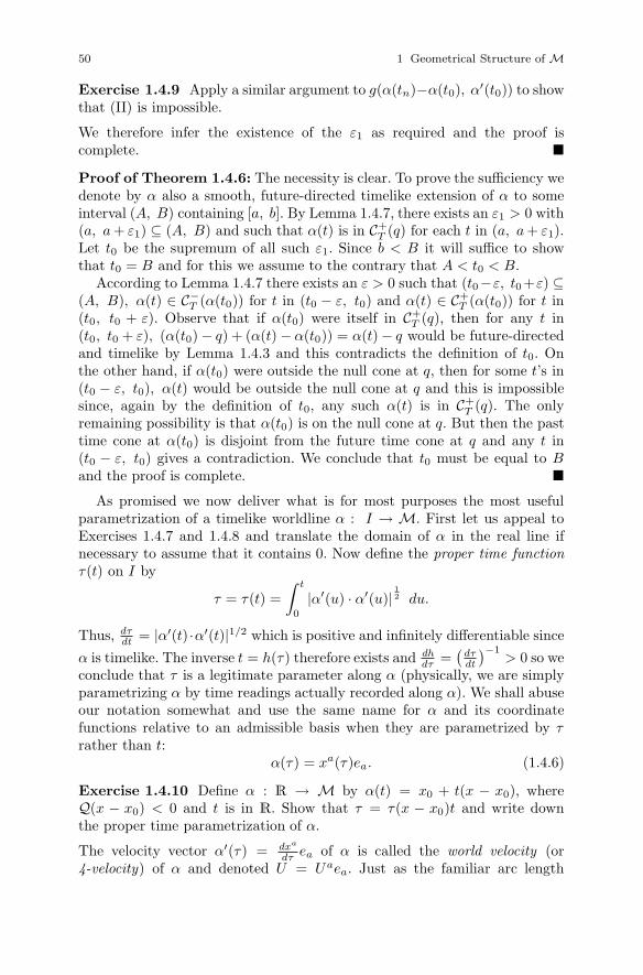
50 1 Geometrical Structure of M
Exercise 1.4.9 Apply a similar argument to g(α(tn)−α(t0), α′(t0)) to showthat (II) is impossible.
We therefore infer the existence of the ε1 as required and the proof iscomplete. �
Proof of Theorem 1.4.6: The necessity is clear. To prove the sufficiency wedenote by α also a smooth, future-directed timelike extension of α to someinterval (A, B) containing [a, b]. By Lemma 1.4.7, there exists an ε1 > 0 with(a, a + ε1) ⊆ (A, B) and such that α(t) is in C+
T (q) for each t in (a, a + ε1).Let t0 be the supremum of all such ε1. Since b < B it will suffice to showthat t0 = B and for this we assume to the contrary that A < t0 < B.
According to Lemma 1.4.7 there exists an ε > 0 such that (t0−ε, t0+ε) ⊆(A, B), α(t) ∈ C−
T (α(t0)) for t in (t0 − ε, t0) and α(t) ∈ C+T (α(t0)) for t in
(t0, t0 + ε). Observe that if α(t0) were itself in C+T (q), then for any t in
(t0, t0 + ε), (α(t0) − q) + (α(t) − α(t0)) = α(t) − q would be future-directedand timelike by Lemma 1.4.3 and this contradicts the definition of t0. Onthe other hand, if α(t0) were outside the null cone at q, then for some t’s in(t0 − ε, t0), α(t) would be outside the null cone at q and this is impossiblesince, again by the definition of t0, any such α(t) is in C+
T (q). The onlyremaining possibility is that α(t0) is on the null cone at q. But then the pasttime cone at α(t0) is disjoint from the future time cone at q and any t in(t0 − ε, t0) gives a contradiction. We conclude that t0 must be equal to Band the proof is complete. �
As promised we now deliver what is for most purposes the most usefulparametrization of a timelike worldline α : I → M. First let us appeal toExercises 1.4.7 and 1.4.8 and translate the domain of α in the real line ifnecessary to assume that it contains 0. Now define the proper time functionτ(t) on I by
τ = τ(t) =∫ t
0
|α′(u) · α′(u)|12 du.
Thus, dτdt = |α′(t) ·α′(t)|1/2 which is positive and infinitely differentiable since
α is timelike. The inverse t = h(τ) therefore exists and dhdτ =
(dτdt
)−1> 0 so we
conclude that τ is a legitimate parameter along α (physically, we are simplyparametrizing α by time readings actually recorded along α). We shall abuseour notation somewhat and use the same name for α and its coordinatefunctions relative to an admissible basis when they are parametrized by τrather than t:
α(τ) = xa(τ)ea. (1.4.6)
Exercise 1.4.10 Define α : R → M by α(t) = x0 + t(x − x0), whereQ(x − x0) < 0 and t is in R. Show that τ = τ(x − x0)t and write downthe proper time parametrization of α.
The velocity vector α′(τ) = dxa
dτ ea of α is called the world velocity (or4-velocity) of α and denoted U = Uaea. Just as the familiar arc length

1.4 Timelike Vectors and Curves 51
parametrization of a curve in R3 has unit speed, so the world velocity of atimelike worldline is always a unit timelike vector.
Exercise 1.4.11 Show that
U · U = −1 (1.4.7)
at each point along α.
The second proper time derivative α′′(τ) = d2xa
dτ2 ea of α is called the worldacceleration (or 4-acceleration) of α and denoted A = Aaea. It is alwaysorthogonal to U and so, in particular, must be spacelike if it is nonzero.
Exercise 1.4.12 Show that
U · A = 0 (1.4.8)
at each point along α. Hint : Differentiate (1.4.7) with respect to τ .
The world velocity and acceleration of a timelike worldline are, as we shallsee, crucial to an understanding of the dynamics of the particle whose world-line is represented by α. A given admissible observer, however, is more likelyto parametrize a particle’s worldline by his time x4 than by τ and so willrequire procedures for calculating U and A from this parametrization. Firstobserve that since α(τ) = (x1(τ), . . . , x4(τ)) is smooth, x4(τ) is infinitely dif-ferentiable. Since α is future-directed, dx4
dτ is positive so the inverse τ = h(x4)exists and h′(x4) = (dx4
dτ)−1 is positive. Thus, x4 is a legitimate parameter
for α. Moreover,
dτ
dx4=∣∣α′(x4) · α′(x4)
∣∣ 12=
√√√√1 −[(
dx1
dx4
)2
+(
dx2
dx4
)2
+(
dx3
dx4
)2]
=√
1 − β2(x4),
where we have denoted by β(x4) the usual instantaneous speed of the particlewhose worldline is α relative to the frame S(x1, x2, x3, x4). Thus,
dx4
dτ= (1 − β2(x4))−
12
which we denote by γ = γ(x4). Now, we compute
U i =dxi
dτ=
dxi
dx4
dx4
dτ= γ
dxi
dx4, i = 1, 2, 3,
andU4 = γ,
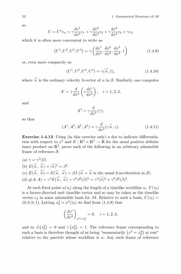
52 1 Geometrical Structure of M
so
U = Uaea = γdx1
dx4e1 + γ
dx2
dx4e2 + γ
dx3
dx4e3 + γe4
which it is often more convenient to write as(U1, U2, U3, U4
)= γ
(dx1
dx4,dx2
dx4,dx3
dx4, 1)
(1.4.9)
or, even more compactly as
(U1, U2, U3, U4) = γ(⇀u, 1), (1.4.10)
where⇀u is the ordinary velocity 3-vector of α in S. Similarly, one computes
Ai = γd
dx4
(γ
dxi
dx4
), i = 1, 2, 3,
and
A4 = γd
dx4(γ),
so that
(A1, A2, A3, A4) = γd
dx4(γ
⇀u, γ). (1.4.11)
Exercise 1.4.13 Using (in this exercise only) a dot to indicate differentia-tion with respect to x4 and E : R3 ×R3 → R for the usual positive definiteinner product on R3, prove each of the following in an arbitrary admissibleframe of reference S:
(a) γ = γ3ββ.
(b) E(⇀u,
⇀u) = |⇀u |2 = β2.
(c) E(⇀u,
⇀u) = E(
⇀u,
⇀a ) = ββ (
⇀a =
⇀u is the usual 3-acceleration in S).
(d) g(A, A) = γ4E(⇀a ,
⇀a ) + γ6β2(β)2 = γ4|⇀a |2 + γ6β2(β)2.
At each fixed point α(τ0) along the length of a timelike worldline α, U(τ0)is a future-directed unit timelike vector and so may be taken as the timelikevector e4 in some admissible basis for M. Relative to such a basis, U(τ0) =(0, 0, 0, 1). Letting x4
0 = x4(τ0) we find from (1.4.9) that(dxi
dx4
)x4=x4
0
= 0, i = 1, 2, 3,
and so β(x4
0
)= 0 and γ
(x4
0
)= 1. The reference frame corresponding to
such a basis is therefore thought of as being “momentarily(x4 = x4
0
)at rest”
relative to the particle whose worldline is α. Any such frame of reference

1.4 Timelike Vectors and Curves 53
is called an instantaneous rest frame for α at α(τ0). Notice that Exer-cise 1.4.12(d) gives
g(A, A) = |⇀a |2 (1.4.12)
in an instantaneous rest frame. Since g(A, A) is invariant under Lorentz trans-formations we find that all admissible observers will agree, at each point alongα, on the magnitude of the 3-acceleration of α relative to its instantaneousrest frames.
As an illustration of these ideas we will examine in some detail the follow-ing situation. A futuristic explorer plans a journey to a distant part of theuniverse. For the sake of comfort he will maintain a constant acceleration of1g (one “earth gravity”) relative to his instantaneous rest frames (assumingthat he neither diets nor overindulges his “weight” will remain the same as onearth throughout the trip). We begin by calculating the explorer’s worldlineα(τ). As usual we denote by U(τ) and A(τ) the world velocity and worldacceleration of α respectively. Thus, (1.4.7), (1.4.8) and (1.4.12) give
U · U = −1, (1.4.13)U · A = 0, (1.4.14)
A · A = g2 (a constant). (1.4.15)
We examine the situation from an admissible frame of reference in which theexplorer’s motion is along the positive x1-axis. Thus, U2 = U3 = A2 = A3 =0and (1.4.13), (1.4.14) and (1.4.15) become
(U1)2 − (U 4)2 = −1, (1.4.16)
U1A1 − U4A4 = 0, (1.4.17)
(A1)2 − (A4)2 = g2. (1.4.18)
Exercise 1.4.14 Solve these last three equations for A1 and A4 to obtainA1 = gU 4 and A4 = gU 1.
The result of Exercise 1.4.14 is a system of ordinary differential equations forU1 and U4. Specifically, we have
dU1
dτ= gU4 (1.4.19)
and
dU4
dτ= gU1. (1.4.20)
Differentiate (1.4.19) with respect to τ and substitute into (1.4.20) to obtain
d2U1
dτ2= g2U1. (1.4.21)
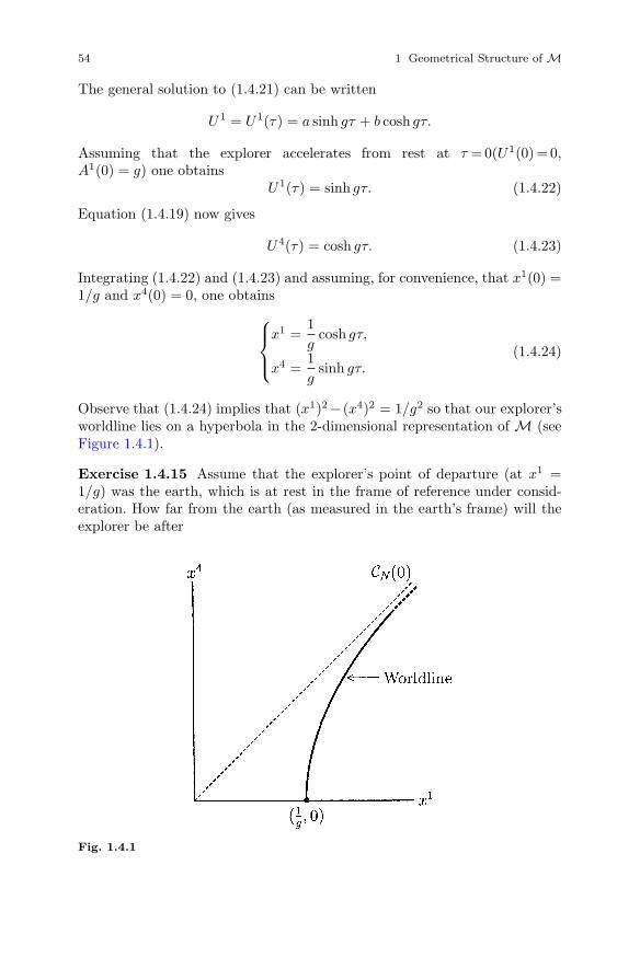
54 1 Geometrical Structure of M
The general solution to (1.4.21) can be written
U1 = U1(τ) = a sinh gτ + b cosh gτ.
Assuming that the explorer accelerates from rest at τ =0(U1(0)=0,A1(0) = g) one obtains
U1(τ) = sinh gτ. (1.4.22)
Equation (1.4.19) now gives
U 4(τ) = cosh gτ. (1.4.23)
Integrating (1.4.22) and (1.4.23) and assuming, for convenience, that x1(0) =1/g and x4(0) = 0, one obtains⎧⎪⎨⎪⎩
x1 =1g
cosh gτ,
x4 =1g
sinh gτ.(1.4.24)
Observe that (1.4.24) implies that (x1)2− (x4)2 = 1/g2 so that our explorer’sworldline lies on a hyperbola in the 2-dimensional representation of M (seeFigure 1.4.1).
Exercise 1.4.15 Assume that the explorer’s point of departure (at x1 =1/g) was the earth, which is at rest in the frame of reference under consid-eration. How far from the earth (as measured in the earth’s frame) will theexplorer be after
Fig. 1.4.1
1.5 Spacelike Vectors 55
(a) 40 years as measured on earth? (How much time will have elapsed on therocket?) Answers : 39 light years (4.38 years).
(b) 40 years as measured on the rocket? (How much time will have elapsedon earth?) Answers : 1017 light years (1017 years).
Hint : It will simplify the arithmetic to measure in light years rather thanmeters. Then g ≈ 1 (light year)−1.
We conclude this section with a theorem which asserts quite generallythat an accelerated observer such as the explorer in the preceding discussionof hyperbolic motion or the “rocket twin” in the twin paradox must alwaysexperience a time dilation not experienced by those of us who remain at restin an admissible frame.
Theorem 1.4.8 Let α : [a, b] → M be a timelike worldline in M fromα(a) = q to α(b) = p. Then
L(α) ≤ τ(p − q) (1.4.25)
and equality holds if and only if α is a parametrization of a timelike straightline joining q and p.
Proof: By Theorem 1.4.6, p − q is timelike and future-directed so we mayselect a basis {ea} with q = x1
0e1 + x20e2 + x3
0e3 + x4qe4, p = x1
0e1 + x20e2 +
x30e3 + x4
pe4 and τ(p − q) = x4p − x4
q = Δx4. Now parametrize α by x4. Then
L(α) =∫ x4
p
x4q
√√√√1 −[(
dx1
dx4
)2
+(
dx2
dx4
)2
+(
dx3
dx4
)2]dx4
≤∫ x4
p
x4q
dx4 = Δx4 = τ(p − q).
Moreover, equality holds if and only if dx i
dx4 = 0 for i = 1, 2, 3, that is, ifand only if xi is constant for i = 1, 2, 3 and this is the case if and only ifα(x4) = x1
0e1 + x20e2 + x3
0e3 + x4e4 for x4q ≤ x4 ≤ x4
p as required. �
1.5 Spacelike Vectors
Now we turn to spacelike separations, i.e., we consider two events x and x0
for which Q(x − x0) > 0. Relative to any admissible basis we have (Δx1)2 +(Δx2)2 +(Δx3)2 > (Δx4)2 so that x−x0 lies outside the null cone at x0 andthere is obviously no admissible basis in which the spatial separation of thetwo events is zero, i.e., there is no admissible observer who can experienceboth events (to do so he would have to travel faster than the speed of light).However, an argument analogous to that given at the beginning of Section 1.4will show that there is a frame in which x and x0 are simultaneous.
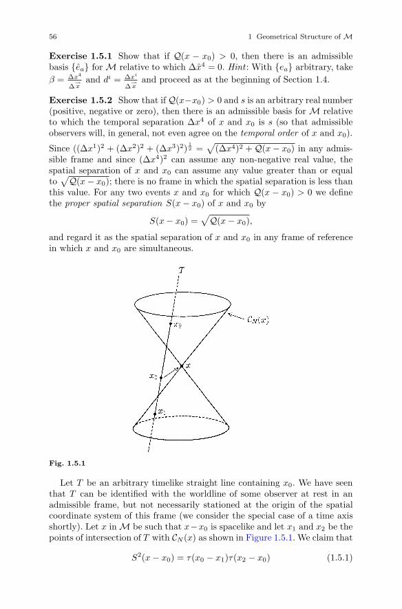
56 1 Geometrical Structure of M
Exercise 1.5.1 Show that if Q(x − x0) > 0, then there is an admissiblebasis {ea} for M relative to which Δx4 = 0. Hint : With {ea} arbitrary, takeβ = Δx4
Δ⇀x
and di = Δxi
Δ⇀x
and proceed as at the beginning of Section 1.4.
Exercise 1.5.2 Show that if Q(x−x0) > 0 and s is an arbitrary real number(positive, negative or zero), then there is an admissible basis for M relativeto which the temporal separation Δx4 of x and x0 is s (so that admissibleobservers will, in general, not even agree on the temporal order of x and x0).
Since ((Δx1)2 + (Δx2)2 + (Δx3)2)12 =√
(Δx4)2 + Q(x − x0) in any admis-sible frame and since (Δx4)2 can assume any non-negative real value, thespatial separation of x and x0 can assume any value greater than or equalto√Q(x − x0); there is no frame in which the spatial separation is less than
this value. For any two events x and x0 for which Q(x − x0) > 0 we definethe proper spatial separation S(x − x0) of x and x0 by
S(x − x0) =√
Q(x − x0),
and regard it as the spatial separation of x and x0 in any frame of referencein which x and x0 are simultaneous.
Fig. 1.5.1
Let T be an arbitrary timelike straight line containing x0. We have seenthat T can be identified with the worldline of some observer at rest in anadmissible frame, but not necessarily stationed at the origin of the spatialcoordinate system of this frame (we consider the special case of a time axisshortly). Let x in M be such that x−x0 is spacelike and let x1 and x2 be thepoints of intersection of T with CN (x) as shown in Figure 1.5.1. We claim that
S2(x − x0) = τ(x0 − x1)τ(x2 − x0) (1.5.1)
1.5 Spacelike Vectors 57
(a result first proved by Robb [R]). To prove (1.5.1) we observe that, sincex − x1 is null,
0 = Q(x − x1) = Q((x0 − x1) + (x − x0)),
0 = −τ2(x0 − x1) + 2(x0 − x1) · (x − x0) + S2(x − x0). (1.5.2)
Similarly, since x2 − x is null,
0 = −τ2(x2 − x0) − 2(x2 − x0) · (x − x0) + S2(x − x0). (1.5.3)
There exists a constant k > 0 such that x2 − x0 = k(x0 − x1) so τ2(x2 −x0) = k2τ2(x0−x1). Multiplying (1.5.2) by k and adding the result to (1.5.3)therefore yields
−(k + k2)τ2(x0 − x1) + (k + 1)S2(x − x0) = 0.
Since k + 1 �= 0 this can be written
S2(x − x0) = kτ2(x0 − x1)= τ(x0 − x1)(kτ(x0 − x1))= τ(x0 − x1)τ(x2 − x0)
as required.Suppose that the spacelike displacement vector x−x0 is orthogonal to the
timelike straight line T . Then (with the notation as above) (x0−x1)·(x−x0) =(x2 − x0) · (x− x0) = 0 so (1.5.2) and (1.5.3) yield S(x− x0) = τ(x2 − x0) =τ(x0 − x1) which we prefer to write as
S(x − x0) = 12(τ(x0 − x1) + τ(x2 − x0)). (1.5.4)
In particular, this is true if T is a time axis. We have seen that, in thiscase, T can be identified with the worldline of an admissible observer O andthe events x and x0 are simultaneous in this observer’s reference frame. Butthen S(x − x0) is the distance in this frame between x and x0. Since x0
lies on T we find that (1.5.4) admits the following physical interpretation:The O-distance of an event x from an admissible observer O is one-half thetime lapse measured by O between the emission and reception of light signalsconnecting O with x.
Exercise 1.5.3 Let x, x0 and x1 be events for which x− x0 and x1 − x arespacelike and orthogonal. Show that
S2(x1 − x0) = S2(x1 − x) + S2(x − x0) (1.5.5)
and interpret the result physically by considering a time axis T which isorthogonal to both x − x0 and x1 − x.
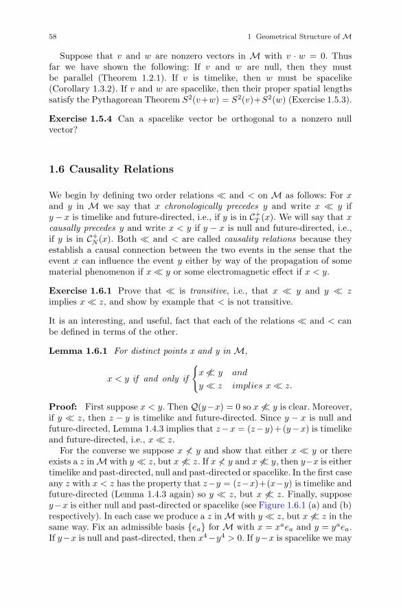
58 1 Geometrical Structure of M
Suppose that v and w are nonzero vectors in M with v · w = 0. Thusfar we have shown the following: If v and w are null, then they mustbe parallel (Theorem 1.2.1). If v is timelike, then w must be spacelike(Corollary 1.3.2). If v and w are spacelike, then their proper spatial lengthssatisfy the Pythagorean Theorem S2(v+w) = S2(v)+S2(w) (Exercise 1.5.3).
Exercise 1.5.4 Can a spacelike vector be orthogonal to a nonzero nullvector?
1.6 Causality Relations
We begin by defining two order relations � and < on M as follows: For xand y in M we say that x chronologically precedes y and write x � y ify − x is timelike and future-directed, i.e., if y is in C+
T (x). We will say that xcausally precedes y and write x < y if y − x is null and future-directed, i.e.,if y is in C+
N (x). Both � and < are called causality relations because theyestablish a causal connection between the two events in the sense that theevent x can influence the event y either by way of the propagation of somematerial phenomenon if x � y or some electromagnetic effect if x < y.
Exercise 1.6.1 Prove that � is transitive, i.e., that x � y and y � zimplies x � z, and show by example that < is not transitive.
It is an interesting, and useful, fact that each of the relations � and < canbe defined in terms of the other.
Lemma 1.6.1 For distinct points x and y in M,
x < y if and only if
{x �� y and
y � z implies x � z.
Proof: First suppose x < y. Then Q(y−x) = 0 so x �� y is clear. Moreover,if y � z, then z − y is timelike and future-directed. Since y − x is null andfuture-directed, Lemma 1.4.3 implies that z−x = (z−y)+(y−x) is timelikeand future-directed, i.e., x � z.
For the converse we suppose x ≮ y and show that either x � y or thereexists a z in M with y � z, but x �� z. If x ≮ y and x �� y, then y−x is eithertimelike and past-directed, null and past-directed or spacelike. In the first caseany z with x < z has the property that z−y = (z−x)+(x−y) is timelike andfuture-directed (Lemma 1.4.3 again) so y � z, but x �� z. Finally, supposey−x is either null and past-directed or spacelike (see Figure 1.6.1 (a) and (b)respectively). In each case we produce a z in M with y � z, but x �� z in thesame way. Fix an admissible basis {ea} for M with x = xaea and y = yaea.If y−x is null and past-directed, then x4−y4 > 0. If y−x is spacelike we may

1.6 Causality Relations 59
Fig. 1.6.1
choose {ea} so that x4−y4 > 0 (Exercise 1.5.2). Now, for each n = 1, 2, 3, . . . ,define zn in M by zn = y1e1 + y2e2 + y3e3 +
(y4 + 1
n
)e4. Then zn − y = 1
ne4
is timelike and future-directed so y � zn for each n. However,
Q(zn − x) = ((zn − y) + (y − x))2
= Q(zn − y) + 2(zn − y) · (y − x) + Q(y − x)
= − 1n2 + 2
n (x4 − y4) + Q(y − x)
= Q(y − x) + 1n
[2(x4 − y4) − 1
n
].
Since Q(y −x) ≥ 0 and x4 − y4 > 0 we can clearly choose n sufficiently largethat Q(zn − x) > 0. For this n, z = zn satisfies y � z, but x �� z. �
Exercise 1.6.2 Show that, for distinct x and y in M,
x � y if and only if
{x ≮ y andx < z < y for some z in M.
A map F : M → M is said to be a causal automorphism if it is one-to-one,onto and both F and F−1 preserve <, i.e., x < y if and only if F (x) < F (y).Note that, in particular, F is not assumed to be linear (or even continuous).We will eventually prove that this actually follows from the definition.
Exercise 1.6.3 Show that a one-to-one map F of M onto M is a causalautomorphism if and only if both F and F−1 preserve �, i.e., x � y if andonly if F (x) � F (y).

60 1 Geometrical Structure of M
We propose next to embark upon a proof of the remarkable result ofZeeman [Z1] to which we referred in the Introduction.1 For the statementof the theorem we define a translation of M to be a map T : M → M ofthe form T (v) = v + v0 for some fixed v0 in M and a dilation to be a mapK : M → M such that K(v) = kv for some positive real number k. An or-thogonal transformation L : M → M is said to be orthochronous if x·Lx < 0for all timelike or null and nonzero x.
Exercise 1.6.4 Show that any translation, dilation, orthochronous orthog-onal transformation, or any composition of such mappings is a causal auto-morphism.
Zeeman’s Theorem asserts that we have just enumerated them all.
Theorem 1.6.2 Let F : M → M be a causal automorphism of M. Thenthere exists an orthochronous orthogonal transformation L : M → M, atranslation T : M → M and a dilation K : M → M such that F = T ◦K ◦L.
For the proof we will require a sequence of five lemmas, the first of which, atleast, is easy.
Lemma 1.6.3 A causal automorphism F : M → M maps light rays to lightrays. More precisely, if x < y and Rx,y is the light ray through x and y, then
F (Rx,y) = RF (x),F (y).
Proof: Since both F and F−1 preserve <, F maps null cones to null conesso F (CN (x)) = CN (F (x)) and F (CN (y)) = CN (F (y)). By Theorem 1.2.2,Rx,y = CN (x) ∩ CN (y) and RF (x),F (y) = CN (F (x)) ∩ CN (F (y)). Thus,
F (Rx,y) = F (CN (x) ∩ CN (y))= F (CN (x)) ∩ F (CN (y))= CN (F (x)) ∩ CN (F (y))= RF (x),F (y). �
Lemma 1.6.4 A causal automorphism F : M → M maps parallel light raysonto parallel light rays.
Proof: Let R1 and R2 be two distinct parallel light rays in M and P the(2-dimensional) plane containing them. Any plane in M is the translation ofa plane through the origin which contains 0, 1 or 2 independent null vectors(depending on whether the plane is outside the null cone to each of its points,tangent to these null cones or intersects all of its time cones). Only the secondtwo cases are relevant to P however.
1The proof is considerably more demanding than anything we have attempted thus far and
might reasonably be omitted on a first reading.

1.6 Causality Relations 61
Suppose first that P contains two independent null directions. Then itcontains two families {Rα} and {Sβ} of light rays with all of the Rα parallelto R1 and R2 and all of the Sβ parallel to some light ray which intersectsboth R1 and R2. Thus, the families {F (Rα)} and {F (Sβ)} are two familiesof light rays in M with the following properties:
1. No two of the F (Rα) intersect.2. No two of the F (Sβ) intersect.3. Each F (Rα) intersects every F (Sβ).
To show that F (R1) and F (R2) are parallel it will suffice (since they do notintersect) to show them coplanar. Suppose not. Then F (R1) and F (R2) liein some 3-dimensional affine subspace R3 of M. Since each F (Sβ) intersectsboth F (R1) and F (R2), it too must lie in R3. Thus, by #3 above, all of theF (Rα) are contained in R3. We claim that, as a result, no F (Rα) can becoplanar with either F (R1) or F (R2) (unless α = 1 or α = 2). For supposeto the contrary that some F (Rα) were coplanar with, say, F (R1). EveryF (Sβ) intersects both F (Rα) and F (R1) so it too must lie in this plane.Since F (R2) does not (by assumption) lie in this plane it can intersect theplane in at most one point. Thus, F (R2) intersects at most one F (Sβ) andthis contradicts #3 above. Consequently, we may select an F (R3) such thatno two of {F (R1), F (R2), F (R3)} are coplanar. Since {F (Sβ)} is then thefamily of straight lines in R3 intersecting all of {F (R1), F (R2), F (R3)} itis the family of generators (rulings) for a hyperboloid of one sheet in R3
(this old, and none-too-well-known, result in analytic geometry is proved onpages 105–106 of [Sa]). In the same way one shows that {F (Rα)} is the otherfamily of rulings for this hyperboloid. But then each F (Rα) would be parallelto some F (Sβ) and this again contradicts #3 above.
Finally, we consider the case in which P contains only one independentnull direction (and so is tangent to each of its null cones). Any point in M hasthrough it a light ray parallel to both R1 and R2. Since the tangent space tothe null cone at each point of R1 is (only) 3-dimensional and since the sameis true of R2 we may select a light ray R3 parallel to both R1 and R2 and notin either of these tangent spaces. Thus, the argument given above applies toR1 and R3 as well as R2 and R3. Consequently, F (R1) and F (R2) are bothparallel to F (R3) and so are parallel to each other. �
Let Rx,y = {x + r(y − x) : r ∈ R} be a light ray and F (Rx,y) = {F (x) +s(F (y) − F (x)) : s ∈ R} its image under F . We regard s as a functionof r : s = f(r). Our next objective is to show that f is linear, i.e., thatf(r + t) = f(r) + f(t) and f(tr) = tf (r) for all r and t in R. First though,a few preliminaries. A map g : Rx,y → Rx,y is called a translation of Rx,y ifthere exists a fixed t in R such that
g(x + r(y − x)) = x + (r + t)(y − x)
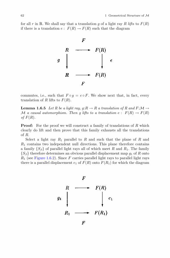
62 1 Geometrical Structure of M
for all r in R. We shall say that a translation g of a light ray R lifts to F (R)if there is a translation e : F (R) → F (R) such that the diagram
commutes, i.e., such that F ◦ g = e ◦F . We show next that, in fact, everytranslation of R lifts to F (R).
Lemma 1.6.5 Let R be a light ray, g:R → R a translation of R and F :M →M a causal automorphism. Then g lifts to a translation e : F (R) → F (R)of F (R).
Proof: For the proof we will construct a family of translations of R whichclearly do lift and then prove that this family exhausts all the translationsof R.
Select a light ray R1 parallel to R and such that the plane of R andR1 contains two independent null directions. This plane therefore containsa family {Sβ} of parallel light rays all of which meet R and R1. The family{Sβ} therefore determines an obvious parallel displacement map g1 of R ontoR1 (see Figure 1.6.2). Since F carries parallel light rays to parallel light raysthere is a parallel displacement e1 of F (R) onto F (R1) for which the diagram
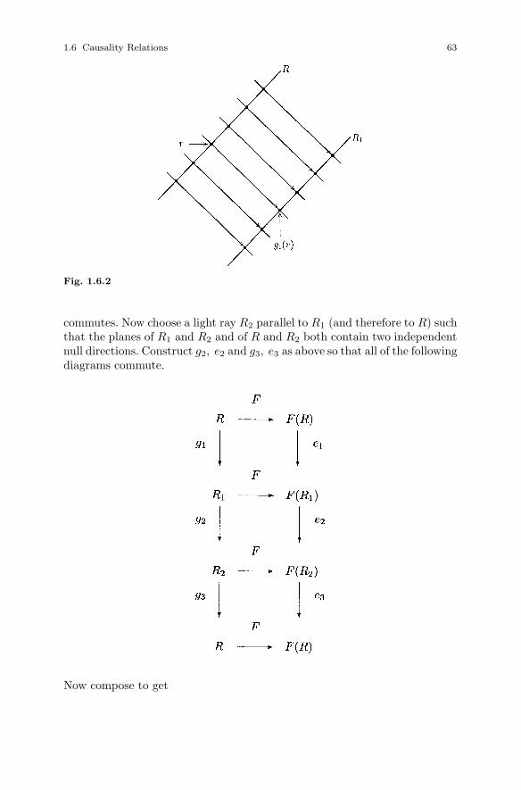
1.6 Causality Relations 63
Fig. 1.6.2
commutes. Now choose a light ray R2 parallel to R1 (and therefore to R) suchthat the planes of R1 and R2 and of R and R2 both contain two independentnull directions. Construct g2, e2 and g3, e3 as above so that all of the followingdiagrams commute.
Now compose to get
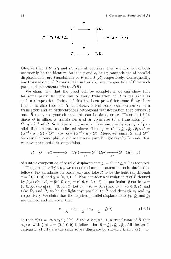
64 1 Geometrical Structure of M
Observe that if R, R1 and R2 were all coplanar, then g and e would bothnecessarily be the identity. As it is g and e, being compositions of paralleldisplacements, are translations of R and F (R) respectively. Consequently,any translation g of R constructed in this way as a composition of three suchparallel displacements lifts to F (R).
We claim now that the proof will be complete if we can show thatfor some particular light ray R every translation of R is realizable assuch a composition. Indeed, if this has been proved for some R we showthat it is also true for R as follows: Select some composition G of atranslation and an orthochronous orthogonal transformation that carries Ronto R (convince yourself that this can be done, or see Theorem 1.7.2).Since G is affine, a translation g of R gives rise to a translation g =G ◦ g ◦G−1 of R. Now represent g as a composition g = g3 ◦ g2 ◦ g1 of par-allel displacements as indicated above. Then g = G−1 ◦ g3 ◦ g2 ◦ g1 ◦G =(G−1 ◦ g3 ◦G) ◦ (G−1 ◦ g2 ◦G) ◦ (G−1 ◦ g3 ◦G). Moreover, since G and G−1
are causal automorphisms and so preserve parallel light rays by Lemma 1.6.4,we have produced a decomposition
R = G−1(R)−−−−→g1
G−1(R1)−−−−→g2
G−1(R2)−−−−→g3
G−1(R) = R
of g into a composition of parallel displacements gi = G−1 ◦ gi ◦G as required.The particular light ray we choose to focus our attention on is obtained as
follows: Fix an admissible basis {ea} and take R to be the light ray throughx = (0, 0, 0, 0) and y = (0, 0, 1, 1). Now consider a translation g of R definedby g(x+r(y−x)) = g(0, 0, r, r) = (0, 0, r+t, r+t). In particular, g carries x =(0, 0, 0, 0) to g(x) = (0, 0, t, t). Let x1 = (0,−t, 0, t) and x2 = (0, 0, 0, 2t) andtake R1 and R2 to be the light rays parallel to R and through x1 and x2
respectively. We claim that the required parallel displacements g1, g2 and g3
are defined and moreover that
x−−−−→g1
x1 −−−−→g2
x2 −−−−→g3
g(x) (1.6.1)
so that g(x) = (g3 ◦ g2 ◦ g1)(x). Since g3 ◦ g2 ◦ g1 is a translation of R thatagrees with g at x = (0, 0, 0, 0) it follows that g = g3 ◦ g2 ◦ g1. All the verifi-cations in (1.6.1) are the same so we illustrate by showing that g1(x) = x1

1.6 Causality Relations 65
Fig. 1.6.3
(see Figure 1.6.3). Note that the plane of R and R1 can contain at most twofamilies of parallel light rays. The light rays parallel to R (and R1) form onesuch family. Since the line joining x and x1 is also null and not parallel to Rit must be in the second family. Thus, g1 exists and, obviously, g1(x) = x1.
�
With Lemma 1.6.5 we can show that a causal automorphism is linear oneach light ray. More precisely, we prove:
Lemma 1.6.6 Let R = {x + r(y − x) : x < y, r ∈ R} be a light ray,F : M → M a causal automorphism and F (R) = {F (x) + s(F (y) − F (x)) :s ∈ R} the image of R under F. Then, regarding s as a function of r, say,s = f(r), we have f(r + t) = f(r) + f(t) and f(tr) = tf (r) for all r and tin R.
Proof: Observe first that f(0) = 0. Now, fix a t in R. We wish to showthat, for any r in R, f(r + t) = f(r) + f(t), i.e., that
F (x + (r + t)(y − x)) = F (x) + (f(r) + f(t))(F (y) − F (x)). (1.6.2)
Let g : R → R denote the translation of R by t, i.e., g(x+r(y−x)) = x+(r+t)(y−x). By Lemma 1.6.5, there exists a translation e : F (R) → F (R) of F (R)such that F ◦g = e◦F . Suppose that e is the translation of F (R) by u = u(t),i.e., that e(F (x) + s(F (y) − F (x))) = F (x) + (s + u(t))(F (y) − F (x)). Then

66 1 Geometrical Structure of M
F (x + (r + t)(y − x)) = F (g(x + r(y − x)))
= F ◦ g(x + r(y − x))
= e ◦ F (x + r(y − x))
= e(F (x) + f(r)(F (y) − F (x)))
= F (x) + [f(r) + u(t)](F (y) − F (x))
so that f(r+t) = f(r)+u(t) for any r. Setting r = 0 gives f(t) = f(0)+u(t) =u(t) so we obtain f(r + t) = f(r) + f(t) as required.
In particular, f(2r) = f(r + r) = f(r) + f(r) = 2f(r) and, by induction,f(nr) = nf (r) for n = 0, 1, 2, . . . . Moreover, f(r) = f(−r + 2r) = f(−r) +2f(r) so f(−r) = −f(r) and, again by induction, f(nr) = nf (r) for n = 0,±1,±2, . . . . If m is also an integer and n is a nonzero integer, nf
(mn r)
=f(mr) = mf (r) so f
(mn r)
= mn f(r). Thus, f(tr) = tf (r) for any rational
number t. Finally, observe that, since F preserves < in M, f preserves < inR and is therefore continuous on R. Since any real number t is the limit ofa sequence of rational numbers we find that f(tr) = tf (r) for any t in R andthe proof is complete. �
We conclude from Lemma 1.6.6 that if Rx,y = {x + r(y − x) : r ∈ R}is a light ray and F is a causal automorphism, then there exists a nonzeroconstant k such that F (Rx,y) = {F (x)+kr (F (y)−F (x)) : r ∈ R}. However,since r = 1 on Rx,y gives y, r = 1 on F (Rx,y) must give F (y) and so k = 1and we have F (Rx,y) = {F (x) + r(F (y) − F (x)) : r ∈ R}.
Lemma 1.6.7 Let F : M → M be a causal automorphism. Then F is anaffine mapping, i.e., its composition with some translation of M (perhaps theidentity) is a linear transformation.
Proof: By first composing with a translation if necessary we may assumethat F (0) = 0 and so the problem is to show that F is linear (the compo-sition of a causal automorphism and a translation is clearly another causalautomorphism).
Select a basis {v1, v2, v3, v4} for M consisting of null vectors (Exercise1.2.1). Define a map G : M → M by
G(y) = G
(4∑
i=1
yivi
)=
4∑i=1
yiF (vi)
for each y =∑4
i=1 yivi (for the remainder of this proof we temporarily sus-pend the summation convention and use a
∑whenever a summation is in-
tended). G is obviously linear and we shall prove that F is linear by showingthat, in fact, F = G. For each i = 1, 2, 3, 4 we let Mi denote the subspaceof M spanned by {vj : j ≤ i}. Thus, M1 is a light ray and M4 is all ofM. We prove F |Mi = G |Mi for all i = 1, 2, 3, 4. For i = 1 this is clear

1.6 Causality Relations 67
Fig. 1.6.4
since F (v1) = G(v1) and, by Lemma 1.6.6, F is linear on M1. Now assumethat i = 2, 3 or 4 and that F |Mi−1 = G |Mi−1. We show from this thatF |Mi = G |Mi as follows: Any y in Mi can be uniquely represented asy = x + yivi, where x is in Mi−1 and there is no sum over i in yivi. Thus,y − x = yivi is null since vi is null. We consider two light rays, the first (R1)through x and y and the second (R2) through 0 and yivi (see Figure 1.6.4).R1 and R2 are parallel so F (R1) and F (R2) are parallel by Lemma 1.6.4.Consequently,
F (R1) = {F (x) + r(F (y) − F (x)) : r ∈ R}
and
F (R2) ={F (0) + r(F (yivi) − F (0)) : r ∈ R
}= {0 + r(F (yivi) − 0) : r ∈ R}.
Since F (R1) and F (R2) are parallel and r = 0 gives 0 on F (R2) and F (x)on F (R1), translation of F (R2) by F (x) gives F (R1). For r = 1 this gives
F (x) + [0 + (F (yivi) − 0)] = F (x) + (F (y) − F (x)),
that is,
F (yivi) = F (y) − F (x).

68 1 Geometrical Structure of M
Thus,
F (y) = F (x) + F (yivi)
= G(x) + F (yivi) since x ∈ Mi−1
= G(x) + yiF (vi) by Lemma 1.6.6
= G(x) + yiG(vi)
= G(x + yivi)= G(y)
and the proof is complete. �
Finally, we are prepared for:
Proof of Theorem 1.6.2: According to Lemma 1.6.7 there is a transla-tion, which we write T−1 : M → M, such that T−1◦F is linear. To completethe proof we need only produce a positive constant 1
ksuch that 1
kT−1 ◦ F
preserves the quadratic form on M. For then, by Lemma 1.2.3, 1k
T−1 ◦ F isa (necessarily orthochronous) orthogonal transformation L. Denoting by Kthe dilation K(v) = kv , 1
kT−1 ◦ F = L therefore gives F = T ◦ K ◦ L as
required.Since both T−1 ◦ F and its inverse take 0 to 0 and preserve <, T−1 ◦ F
must carry the null cone CN (0) onto itself, i.e., Q(x) = 0 if and only ifQ(T−1 ◦F (x)) = 0. Since T−1◦F is linear, both Q(x) and Q(T−1◦F (x)) arequadratic forms and, as we have just observed, they have the same kernel,i.e., vanish for the same x’s. But two indefinite quadratic forms with the samekernel differ at most by a multiplicative constant (Theorem 14.10 of [K]) sothere exists a constant k′ such that Q(x) = k′Q(T−1 ◦ F (x)) for all x. ButT−1 ◦ F is a causal automorphism and so preserves the upper time cone. Inparticular, Q(x) < 0 if and only if Q(T−1 ◦F (x)) < 0, so k′ must be positive.Letting k = (k′)−1/2 we therefore have Q(x) = Q
(1kT−1 ◦ F (x)
)so 1
kT−1◦F
preserves the quadratic form on M and the proof is complete. �
Remark: For those with some basic topology, [Nan] contains a simpleargument that reduces the proof of linearity in Zeeman’s Theorem to anappeal to the so-called Fundamental Theorem of Projective Geometry.
1.7 Spin Transformations and the Lorentz Group
In this section we develop a new and very powerful technique for the con-struction and investigation of Lorentz transformations. The principal tool isa certain homomorphism (called the “spinor map”) from the group of 2 × 2complex matrices with determinant 1 onto the Lorentz group L. With it weuncover a remarkable connection between Lorentz transformations and the
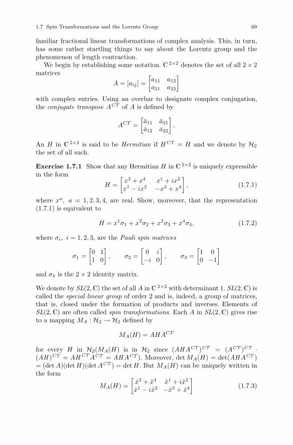
1.7 Spin Transformations and the Lorentz Group 69
familiar fractional linear transformations of complex analysis. This, in turn,has some rather startling things to say about the Lorentz group and thephenomenon of length contraction.
We begin by establishing some notation. C 2×2 denotes the set of all 2× 2matrices
A = [aij ] =[a11 a12
a21 a22
]with complex entries. Using an overbar to designate complex conjugation,the conjugate transpose ACT of A is defined by
ACT =[a11 a21
a12 a22
].
An H in C 2×2 is said to be Hermitian if HCT = H and we denote by H2
the set of all such.
Exercise 1.7.1 Show that any Hermitian H in C 2×2 is uniquely expressiblein the form
H =[
x3 + x4 x1 + ix2
x1 − ix2 −x3 + x4
], (1.7.1)
where xa, a = 1, 2, 3, 4, are real. Show, moreover, that the representation(1.7.1) is equivalent to
H = x1σ1 + x2σ2 + x3σ3 + x4σ4, (1.7.2)
where σi, i = 1, 2, 3, are the Pauli spin matrices
σ1 =[0 11 0
], σ2 =
[0 i−i 0
], σ3 =
[1 00 −1
]and σ4 is the 2 × 2 identity matrix.
We denote by SL(2,C) the set of all A in C 2×2 with determinant 1. SL(2,C) iscalled the special linear group of order 2 and is, indeed, a group of matrices,that is, closed under the formation of products and inverses. Elements ofSL(2,C) are often called spin transformations. Each A in SL(2,C) gives riseto a mapping MA : H2 → H2 defined by
MA(H) = AHACT
for every H in H2(MA(H) is in H2 since (AHACT )CT = (ACT )CT ·(AH )CT = AHCTACT = AHACT ). Moreover, det MA(H) = det(AHACT )= (detA)(det H)(det ACT ) = detH . But MA(H) can be uniquely written inthe form
MA(H) =[
x3 + x4 x1 + ix2
x1 − ix2 −x3 + x4
](1.7.3)

70 1 Geometrical Structure of M
for some real numbers xa, a = 1, 2, 3, 4. Computing the determinants in(1.7.1) and (1.7.2) therefore gives
(x1)2 + (x2)2 + (x3)2 − (x4)2 = (x1)2 + (x2)2 + (x3)2 − (x4)2. (1.7.4)
Thus, the mapping [xa] → [xa] defined by[x3 + x4 x1 + ix2
x1 − ix2 −x3 + x4
]= A
[x3 + x4 x1 + ix 2
x1 − ix 2 −x3 + x4
]ACT , (1.7.5)
which is clearly linear, preserves the quadratic form ηabxaxb. According to
Lemma 1.2.3, the matrix of this map is therefore a general, homogeneousLorentz transformation. We intend to construct this matrix explicitly fromthe entries of
A =[α βγ δ
].
Letting h11 = x3 + x4, h12 = x1 + ix2, h21 = x1 − ix 2, h22 = −x3 + x4 (andh11 = x3 + x4, etc.) we have⎡⎢⎢⎣
h11
h12
h21
h22
⎤⎥⎥⎦ =
⎡⎢⎢⎣0 0 1 11 i 0 01 −i 0 00 0 −1 1
⎤⎥⎥⎦⎡⎢⎢⎣x1
x2
x3
x4
⎤⎥⎥⎦which we will write more compactly as
[hij ] = G [xi]
and similarly for [hij ]. Moreover, it is easy to check that
G−1 =12
⎡⎢⎢⎣0 1 1 00 −i i 01 0 0 −11 0 0 1
⎤⎥⎥⎦ .
Exercise 1.7.2 Write out the product
AHACT =[α βγ δ
] [h11 h12
h21 h22
] [α γβ δ
]explicitly and show that MA(H) = AHACT is equivalent to⎡⎢⎢⎣
h11
h12
h21
h22
⎤⎥⎥⎦ =
⎡⎢⎢⎣αα αβ αβ ββαγ αδ βγ βδαγ βγ αδ βδγγ γδ γδ δδ
⎤⎥⎥⎦⎡⎢⎢⎣h11
h12
h21
h22
⎤⎥⎥⎦
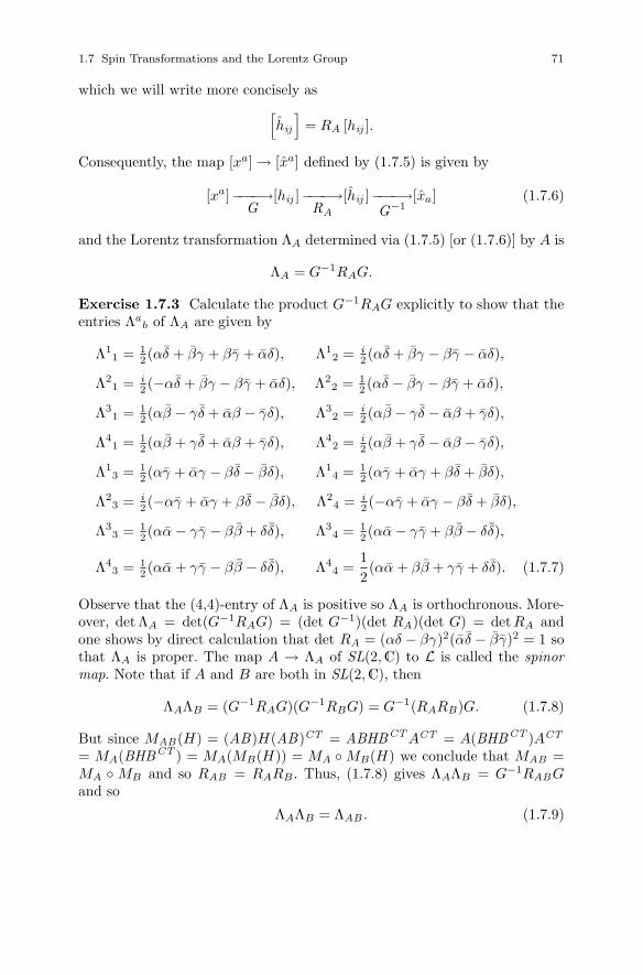
1.7 Spin Transformations and the Lorentz Group 71
which we will write more concisely as[hij
]= RA [hij ].
Consequently, the map [xa] → [xa] defined by (1.7.5) is given by
[xa]−−−−→G
[hij ]−−−−→RA
[hij ]−−−−→G−1
[xa] (1.7.6)
and the Lorentz transformation ΛA determined via (1.7.5) [or (1.7.6)] by A is
ΛA = G−1RAG.
Exercise 1.7.3 Calculate the product G−1RAG explicitly to show that theentries Λa
b of ΛA are given by
Λ11 = 1
2 (αδ + βγ + βγ + αδ), Λ12 = i
2 (αδ + βγ − βγ − αδ),
Λ21 = i
2 (−αδ + βγ − βγ + αδ), Λ22 = 1
2 (αδ − βγ − βγ + αδ),
Λ31 = 1
2 (αβ − γδ + αβ − γδ), Λ32 = i
2 (αβ − γδ − αβ + γδ),
Λ41 = 1
2(αβ + γδ + αβ + γδ), Λ4
2 = i2(αβ + γδ − αβ − γδ),
Λ13 = 1
2(αγ + αγ − βδ − βδ), Λ1
4 = 12(αγ + αγ + βδ + βδ),
Λ23 = i
2(−αγ + αγ + βδ − βδ), Λ2
4 = i2(−αγ + αγ − βδ + βδ),
Λ33 = 1
2(αα − γγ − ββ + δδ), Λ3
4 = 12(αα − γγ + ββ − δδ),
Λ43 = 1
2(αα + γγ − ββ − δδ), Λ4
4 =12(αα + ββ + γγ + δδ). (1.7.7)
Observe that the (4,4)-entry of ΛA is positive so ΛA is orthochronous. More-over, detΛA = det(G−1RAG) = (det G−1)(det RA)(det G) = detRA andone shows by direct calculation that det RA = (αδ − βγ)2(αδ − βγ)2 = 1 sothat ΛA is proper. The map A → ΛA of SL(2,C) to L is called the spinormap. Note that if A and B are both in SL(2,C), then
ΛAΛB = (G−1RAG)(G−1RBG) = G−1(RARB)G. (1.7.8)
But since MAB(H) = (AB)H(AB)CT = ABHBCTACT = A(BHBCT )ACT
= MA(BHBCT ) = MA(MB(H)) = MA ◦ MB(H) we conclude that MAB =MA ◦ MB and so RAB = RARB . Thus, (1.7.8) gives ΛAΛB = G−1RABGand so
ΛAΛB = ΛAB . (1.7.9)
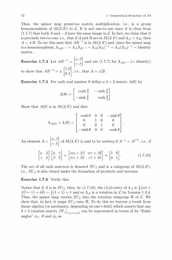
72 1 Geometrical Structure of M
Thus, the spinor map preserves matrix multiplication, i.e., is a grouphomomorphism of SL(2,C) to L. It is not one-to-one since it is clear from(1.7.7) that both A and −A have the same image in L. In fact, we claim that itis precisely two-to-one, i.e., that if A and B are in SL(2,C) and ΛA = ΛB , thenA = ±B. To see this note that AB−1 is in SL(2,C) and, since the spinor mapis a homomorphism, ΛAB−1 = ΛAΛB−1 = ΛA(ΛB)−1 = ΛA(ΛA)−1 = identitymatrix.
Exercise 1.7.4 Let AB−1 =[α βγ δ
]and use (1.7.7) for ΛAB−1 (= identity)
to show that AB−1 = ±[1 00 1
], i.e., that A = ±B.
Exercise 1.7.5 For each real number θ define a 2 × 2 matrix A(θ) by
A(θ) =
[cosh θ
2 − sinh θ2
− sinh θ2 cosh θ
2
].
Show that A(θ) is in SL(2,C) and that
ΛA(θ) = L(θ) =
⎡⎢⎢⎣cosh θ 0 0 − sinh θ0 1 0 00 0 1 0
− sinh θ 0 0 cosh θ
⎤⎥⎥⎦ .
An element A =[α βγ δ
]of SL(2,C) is said to be unitary if A−1 = ACT , i.e., if
[α βγ δ
] [α γβ δ
]=[αα + ββ αγ + βδαγ + βδ γγ + δδ
]=[1 00 1
]. (1.7.10)
The set of all such matrices is denoted SU 2 and is a subgroup of SL(2,C),i.e., SU 2 is also closed under the formation of products and inverses.
Exercise 1.7.6 Verify this.
Notice that if A is in SU 2, then, by (1.7.10), the (4,4)-entry of ΛA is 12(αα +
ββ + γγ + δδ) = 12(1 + 1) = 1 and so ΛA is a rotation in L by Lemma 1.3.4.
Thus, the spinor map carries SU 2 into the rotation subgroup R of L. Weshow that, in fact, it maps SU 2 onto R. To do this we borrow a result fromlinear algebra (or mechanics, depending on one’s field) which asserts that any3 × 3 rotation matrix
[Ri
j
]i,j=1,2,3
can be represented in terms of its “Eulerangles” φ1, θ and φ2 as
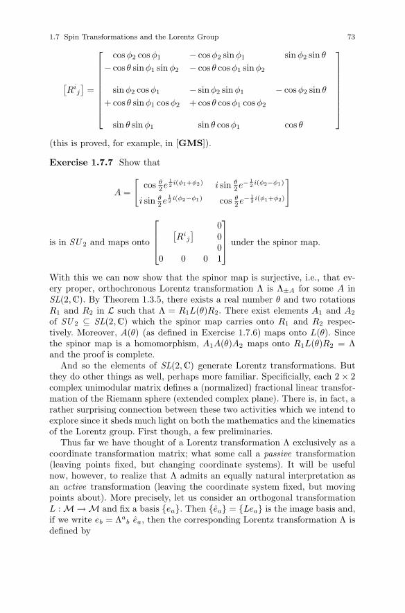
1.7 Spin Transformations and the Lorentz Group 73
[Ri
j
]=
⎡⎢⎢⎢⎢⎢⎢⎢⎢⎣
cosφ2 cosφ1 − cosφ2 sinφ1 sin φ2 sin θ
− cos θ sinφ1 sin φ2 − cos θ cosφ1 sinφ2
sin φ2 cosφ1 − sinφ2 sin φ1 − cosφ2 sin θ
+ cos θ sinφ1 cosφ2 + cos θ cosφ1 cosφ2
sin θ sin φ1 sin θ cosφ1 cos θ
⎤⎥⎥⎥⎥⎥⎥⎥⎥⎦(this is proved, for example, in [GMS]).
Exercise 1.7.7 Show that
A =
[cos θ
2e12 i(φ1+φ2) i sin θ
2e−12 i(φ2−φ1)
i sin θ2e
12 i(φ2−φ1) cos θ
2e−
12 i(φ1+φ2)
]
is in SU 2 and maps onto
⎡⎢⎢⎣0[
Rij
]00
0 0 0 1
⎤⎥⎥⎦ under the spinor map.
With this we can now show that the spinor map is surjective, i.e., that ev-ery proper, orthochronous Lorentz transformation Λ is Λ±A for some A inSL(2,C). By Theorem 1.3.5, there exists a real number θ and two rotationsR1 and R2 in L such that Λ = R1L(θ)R2. There exist elements A1 and A2
of SU 2 ⊆ SL(2,C) which the spinor map carries onto R1 and R2 respec-tively. Moreover, A(θ) (as defined in Exercise 1.7.6) maps onto L(θ). Sincethe spinor map is a homomorphism, A1A(θ)A2 maps onto R1L(θ)R2 = Λand the proof is complete.
And so the elements of SL(2,C) generate Lorentz transformations. Butthey do other things as well, perhaps more familiar. Specificially, each 2 × 2complex unimodular matrix defines a (normalized) fractional linear transfor-mation of the Riemann sphere (extended complex plane). There is, in fact, arather surprising connection between these two activities which we intend toexplore since it sheds much light on both the mathematics and the kinematicsof the Lorentz group. First though, a few preliminaries.
Thus far we have thought of a Lorentz transformation Λ exclusively as acoordinate transformation matrix; what some call a passive transformation(leaving points fixed, but changing coordinate systems). It will be usefulnow, however, to realize that Λ admits an equally natural interpretation asan active transformation (leaving the coordinate system fixed, but movingpoints about). More precisely, let us consider an orthogonal transformationL : M → M and fix a basis {ea}. Then {ea} = {Lea} is the image basis and,if we write eb = Λa
b ea, then the corresponding Lorentz transformation Λ isdefined by
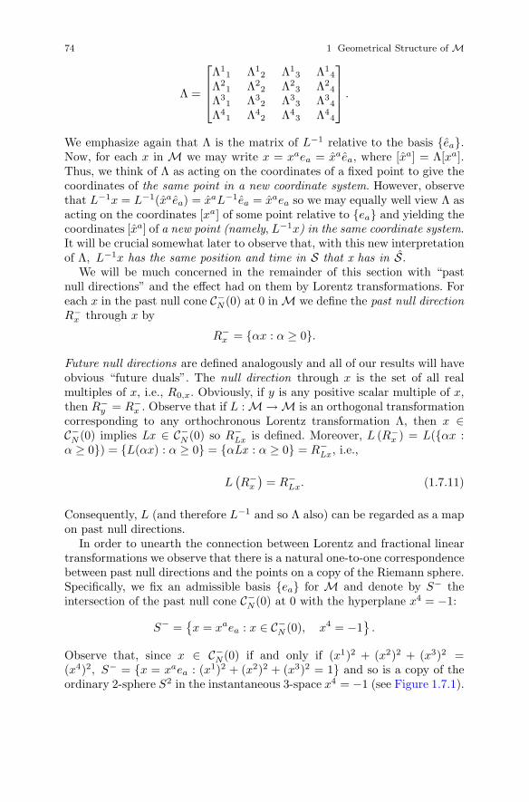
74 1 Geometrical Structure of M
Λ =
⎡⎢⎢⎣Λ1
1 Λ12 Λ1
3 Λ14
Λ21 Λ2
2 Λ23 Λ2
4
Λ31 Λ3
2 Λ33 Λ3
4
Λ41 Λ4
2 Λ43 Λ4
4
⎤⎥⎥⎦ .
We emphasize again that Λ is the matrix of L−1 relative to the basis {ea}.Now, for each x in M we may write x = xaea = xaea, where [xa] = Λ[xa].Thus, we think of Λ as acting on the coordinates of a fixed point to give thecoordinates of the same point in a new coordinate system. However, observethat L−1x = L−1(xaea) = xaL−1ea = xaea so we may equally well view Λ asacting on the coordinates [xa] of some point relative to {ea} and yielding thecoordinates [xa] of a new point (namely, L−1x) in the same coordinate system.It will be crucial somewhat later to observe that, with this new interpretationof Λ, L−1x has the same position and time in S that x has in S.
We will be much concerned in the remainder of this section with “pastnull directions” and the effect had on them by Lorentz transformations. Foreach x in the past null cone C−
N (0) at 0 in M we define the past null directionR−
x through x by
R−x = {αx : α ≥ 0}.
Future null directions are defined analogously and all of our results will haveobvious “future duals”. The null direction through x is the set of all realmultiples of x, i.e., R0,x. Obviously, if y is any positive scalar multiple of x,then R−
y = R−x . Observe that if L : M → M is an orthogonal transformation
corresponding to any orthochronous Lorentz transformation Λ, then x ∈C−
N (0) implies Lx ∈ C−N (0) so R−
Lx is defined. Moreover, L (R−x ) = L({αx :
α ≥ 0}) = {L(αx) : α ≥ 0} = {αLx : α ≥ 0} = R−Lx , i.e.,
L(R−
x
)= R−
Lx. (1.7.11)
Consequently, L (and therefore L−1 and so Λ also) can be regarded as a mapon past null directions.
In order to unearth the connection between Lorentz and fractional lineartransformations we observe that there is a natural one-to-one correspondencebetween past null directions and the points on a copy of the Riemann sphere.Specifically, we fix an admissible basis {ea} for M and denote by S− theintersection of the past null cone C−
N(0) at 0 with the hyperplane x4 = −1:
S− ={x = xaea : x ∈ C−
N (0), x4 = −1}
.
Observe that, since x ∈ C−N(0) if and only if (x1)2 + (x2)2 + (x3)2 =
(x4)2, S− = {x = xaea : (x1)2 + (x2)2 + (x3)2 = 1} and so is a copy of theordinary 2-sphere S2 in the instantaneous 3-space x4 = −1 (see Figure 1.7.1).
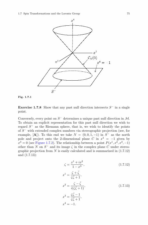
1.7 Spin Transformations and the Lorentz Group 75
Fig. 1.7.1
Exercise 1.7.8 Show that any past null direction intersects S− in a singlepoint.
Conversely, every point on S− determines a unique past null direction in M.To obtain an explicit representation for this past null direction we wish toregard S− as the Riemann sphere, that is, we wish to identify the pointsof S− with extended complex numbers via stereographic projection (see, forexample, [A]). To this end we take N = (0, 0, 1,−1) in S− as the northpole and project onto the 2-dimensional plane C in x4 = −1 given byx3 = 0 (see Figure 1.7.2). The relationship between a point P (x1, x2, x3,−1)other than N on S− and its image ζ in the complex plane C under stereo-graphic projection from N is easily calculated and is summarized in (1.7.12)and (1.7.13):
ζ =x1 + ix2
1 − x3, (1.7.12)
x1 =ζ + ζ
ζζ + 1,
x2 =ζ − ζ
i(ζζ + 1), (1.7.13)
x3 =ζζ − 1ζζ + 1
,
x4 = −1.
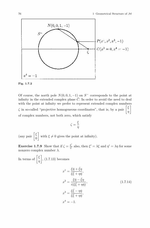
76 1 Geometrical Structure of M
Fig. 1.7.2
Of course, the north pole N(0, 0, 1,−1) on S− corresponds to the point atinfinity in the extended complex plane C. In order to avoid the need to dealwith the point at infinity we prefer to represent extended complex numbers
ζ in so-called “projective homogeneous coordinates”, that is, by a pair[
ξη
]of complex numbers, not both zero, which satisfy
ζ =ξ
η
(any pair[
ξ0
]with ξ �= 0 gives the point at infinity).
Exercise 1.7.9 Show that if ζ = ξ′
η′ also, then ξ′ = λξ and η′ = λη for somenonzero complex number λ.
In terms of[
ξη
], (1.7.13) becomes
x1 =ξη + ξη
ξξ + ηη,
x2 =ξη − ξη
i(ξξ + ηη), (1.7.14)
x3 =ξξ − ηη
ξξ + ηη,
x4 = −1.
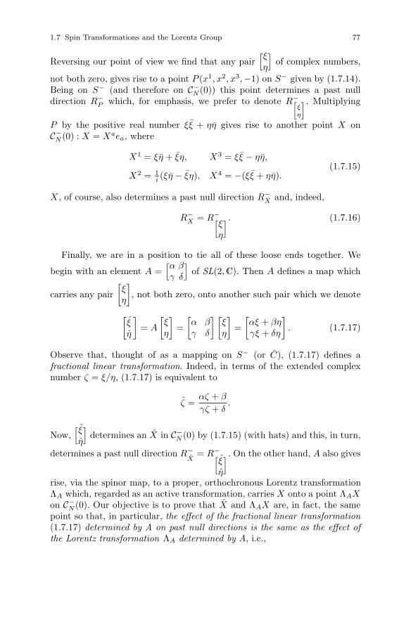
1.7 Spin Transformations and the Lorentz Group 77
Reversing our point of view we find that any pair[ξη
]of complex numbers,
not both zero, gives rise to a point P (x1, x2, x3,−1) on S− given by (1.7.14).Being on S− (and therefore on C−
N (0)) this point determines a past nulldirection R−
P which, for emphasis, we prefer to denote R−[ξη
]. Multiplying
P by the positive real number ξξ + ηη gives rise to another point X onC−
N (0) : X = Xaea, where
X1 = ξη + ξη, X3 = ξξ − ηη,
X2 = 1i (ξη − ξη), X4 = −(ξξ + ηη).
(1.7.15)
X , of course, also determines a past null direction R−X and, indeed,
R−X = R−[
ξη
]. (1.7.16)
Finally, we are in a position to tie all of these loose ends together. We
begin with an element A =[α βγ δ
]of SL(2,C). Then A defines a map which
carries any pair[ξη
], not both zero, onto another such pair which we denote
[ξη
]= A
[ξη
]=[α βγ δ
] [ξη
]=[αξ + βηγξ + δη
]. (1.7.17)
Observe that, thought of as a mapping on S− (or C), (1.7.17) defines afractional linear transformation. Indeed, in terms of the extended complexnumber ζ = ξ/η, (1.7.17) is equivalent to
ζ =αζ + β
γζ + δ.
Now,[ξη
]determines an X in C−
N (0) by (1.7.15) (with hats) and this, in turn,
determines a past null direction R−X
= R−[ξη
]. On the other hand, A also gives
rise, via the spinor map, to a proper, orthochronous Lorentz transformationΛA which, regarded as an active transformation, carries X onto a point ΛAXon C−
N (0). Our objective is to prove that X and ΛAX are, in fact, the samepoint so that, in particular, the effect of the fractional linear transformation(1.7.17) determined by A on past null directions is the same as the effect ofthe Lorentz transformation ΛA determined by A, i.e.,

78 1 Geometrical Structure of M
R−⎡⎣ ξη
⎤⎦ = R−ΛAX . (1.7.18)
To prove all of this we proceed as follows: Begin by solving (1.7.15) for thefour products ξη, ξη, ξξ and ηη to obtain
ξξ = 12
(X3 + X4
), ξη = 1
2 (X1 + iX2),
ξη = 12
(X1 − iX2
), ηη = 1
2 (−X3 + X4),
so that
12
[X3 + X4 X1 + iX2
X1 − iX2 −X3 + X4
]=[ξξ ξηξη ηη
]=[ξη
] [ξ η]. (1.7.19)
Now perform the unimodular transformation (1.7.17) to obtain[ξη
]. The
corresponding point X = Xaea given by (1.7.15) with hats must satisfy(1.7.19) with hats, i.e.,
12
[X3 + X4 X1 + iX2
X1 − iX2 −X3 + X4
]=
12
[X3 + X4 X1 + iX2
X1 − iX2 −X3 + X4
]CT
=[[
ξη
] [ ¯ξ ¯η]]CT
=[ ¯ξ ¯η]CT
[ξη
]CT
=[ξη
] [A
[ξη
]]CT
= A
[ξη
] [ξη
]CT
ACT
= A
[[ξη
][ξ η]]ACT
=12A
[X3 + X4 X1 + iX 2
X1 − iX 2 −X3 + X4
]ACT .
Thus,[X3 + X4 X1 + iX2
X1 − iX2 −X3 + X4
]= A
[X3 + X4 X1 + iX 2
X1 − iX 2 −X3 + X4
]ACT . (1.7.20)
Comparing (1.7.20) and (1.7.5) and the definition of ΛA we find that, indeed,
X = ΛAX,
so that (1.7.18) is proved.
1.7 Spin Transformations and the Lorentz Group 79
Since the spinor map is surjective, every element of L is ΛA for some A inSL(2, C) and so every element of L determines a fractional linear transfor-mation of S− which has the same effect on past null directions (±A give riseto the same fractional linear transformation). Conversely, since the past nullvectors span M (reconsider Exercise 1.2.1 and select only past-directed vec-tors), a Lorentz transformation is completely determined by its effect on pastnull directions. Some consequences of this correspondence between elementsof L and fractional linear transformations of S− are immediate.
Theorem 1.7.1 A proper, orthochronous Lorentz transformation, if not theidentity, leaves invariant at least one and at most two past null directions.
This follows at once from the familiar fact that any fractional linear trans-formation of the Riemann sphere, if not the identity, has two (possibly co-incident) fixed points (see [A]). Another well-known property of fractionallinear transformations is that they are completely determined by their valueson any three distinct points in the extended complex plane (see [A]). Hence:
Theorem 1.7.2 A proper, orthochronous Lorentz transformation is com-pletely determined by its effect on any three distinct past null directions. Moreprecisely, given two sets of three distinct past null directions there is one andonly one element of L which carries the first set (one-to-one) onto the sec-ond set.
As our final application we will derive a remarkable result of Penrose[Pen1] related to what has been called the “invisibility of the Lorentz contrac-tion”. An admissible observerO “observes” in a quite specific and well-definedway. One pictures the observer’s frame of reference as a spatial coordinategrid with clocks located at the lattice points of the grid and either recordingdevices or assistants stationed with the clocks to take all of the required localreadings. O then “observes”, say, a moving sphere by either turning on thedevices or alerting the assistants to record the arrival times at their locationsof various points on the sphere. When things have calmed down again O willcollect all of this data for analysis. He may then, for example, construct a“picture” of the sphere by selecting (arbitrarily) some instant of his time,collecting together all of the locations in his frame which recorded the pas-sage of a point on the boundary of the sphere at that instant and “plotting”these points in his frame. In this way he will find himself constructing, not asphere, but an ellipsoid due to length contraction in the direction of motion.
What our observer O actually “sees” (through his eye or a camera lens),however, is not so straightforward. We wish to construct an (admittedly ide-alized) geometrical representation in M of this “field of vision”.
It is a clear evening and, as you stroll outside, you glance up and seethe Big Dipper. More precisely, you direct the surface of your eye toward agroup of incoming photons (idealize and assume one from each star in theconstellation). Regardless of when they left their sources these photons arriveat this surface simultaneously (in your reference frame) and thereby create
80 1 Geometrical Structure of M
a pattern (image) which is recorded by your brain. This pattern is whatyou “see”. Where can we find it in M? Each of the photons you see has aworldline in M which lies along the past null cone C−
N (0) (you are locatedat the origin of your coordinate system and the image is registered in yourbrain at x4 = 0). Just slightly before x4 = 0 the photons impacted the surfaceof your eye and formed their image. At x4 = −1 the photons were all on asphere of radius 1 about the origin of your coordinate system and formed onthis sphere the same pattern that your eye registered a bit later. Projectingthis image down to the plane x4 = −1 in M we find the worldlines of thesephotons intersecting S− in the very image that you “see”. As a geometricalrepresentation of what you see (at the event x1 = x2 = x3 = x4 = 0) wetherefore take the intersections with S− of the worldlines of all the photonsthat trigger your brain to record an image at x4 = 0.
Now we ask the following question. Suppose that what you see is not theBig Dipper, but something with a circular outline, e.g., a sphere at rest inyour reference frame. What is seen by another admissible observer, movingrelative to your frame, but momentarily coincident with you at the origin?According to the new observer the sphere is moving and so certainly must“appear” contracted in the direction of motion. Surely, he must “see” anelliptical, not a circular image.
But he does not! We propose to argue that, despite the Lorentz contractionin the direction of motion, the sphere will still present a circular outlineto O (although, in a degenerate case, the circle may “appear” straight).Indeed, this is merely a reflection of yet another familiar property of fractionallinear transformations of the Riemann sphere: they carry circles onto circles.Thus, if Λ is the Lorentz transformation relating S and S, then, regardedas an active transformation on past null directions, it carries any family ofsuch null directions which intersect S− in a circle onto another such family.In somewhat more detail we recall (page 74) that, for each x in M, Λ(x)(= L−1(x)) has the same position and time in S that x has in S. In particular,Λ(x) ∈ S− if and only if x ∈ S−. Thus, Λ (R−
x ) = R−Λ(x) “looks the same”
to O at x4 = 0 as R−x “looks” to O at x4 = 0 (same relative position in the
sky). Now, if we have a family N of past null directions (forming a certain“image” for O at x4 = 0) it follows that the appearance of this image for Oat x4 = 0 will be the same as the appearance of Λ(N ) to O at x4 = 0. Ifthe rays in N present a circular outline to O at x4 = 0, so will Λ(N ) andtherefore O will also see a circular outline at x4 = 0. O and O both “see” acircular outline.
Exercise 1.7.10 Describe the “degenerate case” in which the circle“appears” straight.
Exercise 1.7.11 Offer a plausible physical explanation for this “invisibilityof the Lorentz contraction”. Hint : For O the photons which arrive simul-taneously at the surface of his eye to form their image also left the spheresimultaneously. Is this true for O?

1.8 Particles and Interactions 81
1.8 Particles and Interactions
A billiard ball rolling with constant speed in a straight line collides withanother billiard ball, initially at rest, and the two balls rebound from theimpact. The actual physical mechanisms involved in such an interaction arequite complicated, having to do with the electrical repulsion between elec-trons in the atoms at the surfaces of the two balls. Nevertheless, much canbe said about the motion which results from such a collision even withoutdetailed information about this electromagnetic interaction. What makes thispossible is the idea (one of the most profound and powerful in all of physics)that such situations are often governed by conservation laws. Specifically,the conservation of Newtonian momentum has immediate implications forthe motion of our billiard balls (for example, that, assuming the collision isglancing rather than head-on, they will separate along paths that form a rightangle) and these predictions were well borne out by observation, at least untilthe 20th century. However, Newtonian physics would make precisely the samepredictions if the billiard balls were replaced by protons travelling at speedscomparable to that of light and here the observational evidence does notsupport these conclusions (e.g., the protons generally separate along pathswhich form an angle less than 90◦). In this section we shall investigate therelativistic alternative to the classical principles of the conservation of mo-mentum and energy and draw some elementary consequences from it. First,though, some definitions.
A material particle in M is a pair (α, m), where α : I → M is a timelikeworldline parametrized by proper time τ and m is a positive real numbercalled the particle’s proper mass (and is to be identified intuitively with the“inertial mass” of the particle from Newtonian mechanics). (α, m) is called afree material particle if α is of the form α(τ) = x0 + τU for some fixed eventx0 and unit timelike vector U . Recall that, for any timelike worldline α(τ)the proper time derivative α′(τ) is called the world velocity of α and denotedU = U(τ). The world momentum (or 4-momentum) of (α, m) is denoted Pand defined by
P = P (τ) = mU (τ).
Notice that, since U · U = −1 (Exercise 1.4.11), we have
P · P = −m2. (1.8.1)
Now fix an arbitrary admissible basis {ea}. Writing P = P aea and usingnotation analogous to that established in (1.4.9) and (1.4.10) we have
P = (P 1, P 2, P 3, P 4) = mγ(⇀u, 1) = (
⇀p , mγ),
where⇀p = (P 1, P 2, P 3) is called the relative 3-momentum of (α, m) in {ea}.
Notice that if γ = ( 1− β2)−12 is near 1, i.e., if the speed of (α, m) relative to
{ea} is small, then⇀p is approximately equal to m
⇀u , the classical Newtonian
82 1 Geometrical Structure of M
momentum of (α, m) in {ea}. The quantity mγ = m√1−β2
is sometimes re-
ferred to as the “relativistic mass” of (α, m) relative to {ea} since it permitsone to retain a formal similarity between the Newtonian and relativistic def-initions of momentum (“mass times velocity”). Inertial mass was regardedin classical physics as a measure of the particle’s resistance to acceleration.From the relativistic point of view this resistance must become unboundedas β → 1 and mγ certainly has this property. We prefer, however, to avoidthe quite misleading attitude that “mass increases with velocity” and simplyabandon the Newtonian view that momentum is a linear function of velocity.
We shall denote by |⇀p | the usual Euclidean magnitude of the relative
3-momentum in {ea}, i.e., |⇀p |2 = (P 1)2 +(P 2)2 + (P 3)2. To see more clearly
the relationship between P and more familiar Newtonian concepts we use thebinomial expansion
γ = (1 − β2)−12 = 1 + 1
2β2 + 3
8β4 + · · · (1.8.2)
of γ (valid since |β | < 1) to write
P i = mγui = mui + 12muiβ2 + · · · , i = 1, 2, 3, and (1.8.3)
P 4 = mγ = m + 12mβ2 + · · · . (1.8.4)
The nonlinear terms in (1.8.3) are absent from the Newtonian definition, butare crucial to the relativistic theory since they force |
⇀p | to become unbounded
as β → 1, i.e., they impose the “speed limit” on material particles relative toadmissible frames of reference.
The physical interpretation of (1.8.4) is much more interesting. Notice,in particular, the appearance of the term 1
2mβ2 corresponding to the clas-
sical kinetic energy. The presence of this term leads us to call P 4 the totalrelativistic energy of (α, m) in {ea} and denote it E.
E = −P · e4 = P 4 = mγ = m + 12mβ2 + · · · . (1.8.5)
Exercise 1.8.1 Show that, relative to any admissible basis {ea},
m2 = E2 − |⇀p |2. (1.8.6)
A few words of caution are in order here. The concept of “energy” in clas-sical physics is quite a subtle one. Many different types of energy are de-fined in different situations, but each is in one way or another intuitivelyrelated to a system’s “ability to do work”. Now, simply calling P 4 the totalrelativistic energy of our particle does not ensure that this intuitive inter-pretation is still valid. Whether or not the name is appropriate can only bedetermined experimentally. In particular, one should determine whether or
1.8 Particles and Interactions 83
not the presence of the term m in (1.8.5) is consistent with this interpreta-tion. Observe that when β = 0 (i.e., in the instantaneous rest frame of theparticle) P 4 = E = m (= mc2 in traditional units) so that even when theparticle is at rest relative to an admissible frame it still has “energy” in thisframe, the amount being numerically equal to m. If this is really “energy”in the classical sense, it should be capable of doing work, i.e., it should bepossible to “liberate” (and use) it. That this is indeed possible is demon-strated daily in particle physics laboratories and, fortunately not so often, inthe explosion of atomic and nuclear bombs.
It is remarkable that the classically distinct concepts of momentum, energyand mass find themselves so naturally integrated into the single relativisticnotion of world momentum (energy-momentum). We ask the reader to showthat the process was indeed natural in the sense that if one believes thatrelativistic momentum should be represented by a vector in M and that thefirst three components of P = mU are “right”, then one has no choice aboutthe fourth component.
Exercise 1.8.2 Show that two vectors v and w in M with the same spatialcomponents relative to every admissible basis (i.e., v1 = w1, v2 = w2 andv3 = w3 for every {ea}) must, in fact, be equal. Hint : It will be enough toshow that a vector whose first three components are zero in every admissiblecoordinate system must be the zero vector.
Special relativity is of little interest to those who study colliding billiardballs (the relative speeds are so small that any “relativistic effects” are negli-gible). On the other hand, when the colliding objects are elementary particles(protons, neutrons, electrons, mesons, etc.) these relativistic effects are thedominant features. Such interactions between elementary particles, however,very often involve not only material particles, but photons as well and we wishto include these in our study. Now, a photon is, in many ways, analogous toa free material particle. Relative to any admissible frame of reference it trav-els along a straight line with constant speed, i.e., it has a linear worldline.Since this worldline is null, however, it has no proper time parametrizationand so no world velocity. Nevertheless, photons do possess “momentum” and“energy” and so should have a “world momentum” (witness, for example, thephotoelectric effect in which photons collide with and eject electrons fromtheir orbits in an atom). Unlike a material particle, however, the photon’scharacteristic feature is not mass, but energy (frequency, wavelength) andthis is highly observer-dependent (e.g., wavelengths of photons emitted fromthe atoms of a star are “red-shifted” (lengthened) relative to those measuredon earth for the same atoms because the stars are receding from us due to theexpansion of the universe). A hint as to how these features can be modelledin M is provided by:
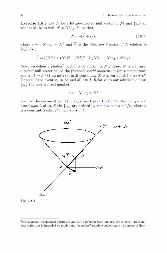
84 1 Geometrical Structure of M
Exercise 1.8.3 Let N be a future-directed null vector in M and {ea} anadmissible basis with N = Naea. Show that
N = ε(⇀e + e4), (1.8.7)
where ε = −N · e4 = N4 and⇀e is the direction 3-vector of N relative to
{ea}, i.e.,
⇀e = ((N1)2 + (N 2)2 + (N3)2)−
12 (N1e1 + N2e2 + N3e3).
Now, we define a photon2 in M to be a pair (α, N), where N is a future-directed null vector called the photon’s world momentum (or 4-momentum)and α : I → M (I an interval in R containing 0) is given by α(t) = x0 + tNfor some fixed event x0 in M and all t in I. Relative to any admissible basis{ea} the positive real number
ε = −N · e4 = N4
is called the energy of (α, N) in {ea} (see Figure 1.8.1). The frequency ν andwavelength λ of (α, N) in {ea} are defined by ν = ε/h and λ = 1/ν, where his a constant (called Planck’s constant).
Fig. 1.8.1
2No quantum mechanical subtleties are to be inferred from our use of the term “photon”.Our definition is intended to model any “massless” particle travelling at the speed of light.
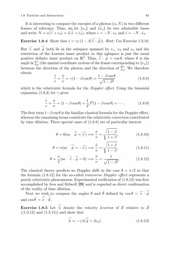
1.8 Particles and Interactions 85
It is interesting to compare the energies of a photon (α, N) in two differentframes of reference. Thus, we let {ea} and {ea} be two admissible basesand write N = ε(
⇀e + e4) = ε(
⇀
e + e4), where ε = −N · e4 and ε = −N · e4.
Exercise 1.8.4 Show that ε = γε (1− β(⇀e ·
⇀
d )). Hint : Use Exercise 1.3.10.
But⇀e and
⇀
d both lie in the subspace spanned by e1, e2 and e3 and therestriction of the Lorentz inner product to this subspace is just the usualpositive definite inner product on R3. Thus,
⇀e ·
⇀
d = cos θ, where θ is theangle in
∑(the spatial coordinate system of the frame corresponding to {ea})
between the direction of the photon and the direction of∑
. We thereforeobtain
ε
ε=
ν
ν= γ(1 − β cos θ) =
1 − β cos θ√1 − β2
(1.8.8)
which is the relativistic formula for the Doppler effect. Using the binomialexpansion (1.8.2) for γ gives
ε
ε=
ν
ν= (1 − β cos θ) +
12β2(1 − β cos θ) + · · · . (1.8.9)
The first term 1−β cos θ is the familiar classical formula for the Doppler effect,whereas the remaining terms constitute the relativistic correction contributedby time dilation. Three special cases of (1.8.8) are of particular interest.
θ = 0(so⇀
d =⇀e ) =⇒ ν
ν=
√1 − β
1 + β, (1.8.10)
θ = π(so⇀
d = −⇀e ) =⇒ ν
ν=
√1 + β
1 − β, (1.8.11)
θ =π
2(so
⇀e ·
⇀
d = 0) =⇒ ν
ν=
1√1 − β2
. (1.8.12)
The classical theory predicts no Doppler shift in the case θ = π/2 so thatthe formula (1.8.12) for the so-called transverse Doppler effect represents apurely relativistic phenomenon. Experimental verification of (1.8.12) was firstaccomplished by Ives and Stilwell [IS] and is regarded as direct confirmationof the reality of time dilation.
Next we wish to compare the angles θ and θ defined by cos θ =⇀e ·
⇀
d
and cos θ =⇀
e ·⇀
d .
Exercise 1.8.5 Let⇀
u denote the velocity 3-vector of S relative to S((1.3.12) and (1.3.15)) and show that
⇀
u = −γβ(⇀
d + βe4). (1.8.13)
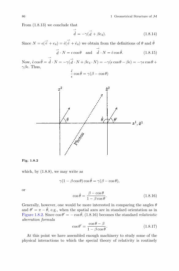
86 1 Geometrical Structure of M
From (1.8.13) we conclude that⇀
d = −γ(⇀
d + βe4). (1.8.14)
Since N = ε(⇀e + e4) = ε(
⇀
e + e4) we obtain from the definitions of θ and θ
⇀
d · N = ε cos θ and⇀
d · N = ε cos θ. (1.8.15)
Now, ε cos θ =⇀
d ·N = −γ(⇀
d ·N + βe4 ·N) = −γ(ε cos θ − βε) = −γε cos θ +γβε. Thus,
ε
εcos θ = γ(β − cos θ)
Fig. 1.8.2
which, by (1.8.8), we may write as
γ(1 − β cos θ) cos θ = γ(β − cos θ),
orcos θ =
β − cos θ
1 − β cos θ. (1.8.16)
Generally, however, one would be more interested in comparing the angles θand θ′ = π − θ, e.g., when the spatial axes are in standard orientation as inFigure 1.8.2. Since cos θ′ = − cos θ, (1.8.16) becomes the standard relativisticaberration formula
cos θ′ =cos θ − β
1 − β cos θ. (1.8.17)
At this point we have assembled enough machinery to study some of thephysical interactions to which the special theory of relativity is routinely
1.8 Particles and Interactions 87
applied. Henceforth, we shall use the term free particle to refer to either afree material particle or a photon. If A is a finite set of free particles, theneach element of A has a unique world momentum vector. The sum of thesevectors is called the total world momentum (or total 4-momentum) of A.A contact interaction in M is a triple (A, x, A), where A and A are twofinite sets of free particles, neither of which contains a pair of particles withlinearly dependent world momenta, and x is an event such that
(a) x is the terminal point of all the particles in A (i.e., for each (α, m) in Awith α : [a, b] → M, we have α(b) = x),
(b) x is the initial point of all the particles in A, and(c) the total world momentum of A equals the total world momentum of A.
Intuitively, the event x should be regarded as the collision of all the particlesin A, from which emerge all the particles in A (which may be physicallyquite different than those in A, e.g., it has been observed that the collision oftwo electrons can result in three electrons and a positron). The prohibitionon pairs of particles with linearly dependent world momenta in the same setis based on the presumption that two such particles would be physically in-distinguishable. Property (c) is called the conservation of world momentumand contains the appropriate relativistic generalizations of two classical con-servation principles: the conservation of momentum and the conservation ofenergy.
Several conclusions concerning contact interactions can be drawn directlyfrom the results we have available. Consider, for example, an interaction(A, x, A) in which A consists of a single photon. Then the total world mo-mentum of A is null so the same must be true of A. Since the world momentaof the individual particles in A are all either timelike or null and all are future-directed, Lemma 1.4.3 implies that all of these world momenta must be nulland parallel. Since A cannot contain two distinct photons with parallel worldmomenta, A must also consist of a single photon which, by (c), must have thesame world momentum as the photon in A. In essence, “nothing happenedat x”. We conclude that no nontrivial interaction of the type modelled by ourdefinition can result in a single photon and nothing else.
A contact interaction (A, x, A) is called a disintegration or decay if Aconsists of a single free particle.
Exercise 1.8.6 Analyze a disintegration (A, x, A) in which A consists of asingle photon.
Suppose that A consists of a single free material particle of proper massm0 and A consists of two material particles with proper masses m1 and m2
(such disintegrations do, in fact, occur in nature, e.g., in α-emission). LetP0, P1 and P2 be the world momenta of the particles with masses m0, m1
and m2 respectively. Appealing to (1.8.1), the Reversed Triangle Inequality

88 1 Geometrical Structure of M
(Theorem 1.4.2) and the fact that P1 and P2 are linearly independent wefind that
m0 > m1 + m2. (1.8.18)
The excess mass m0 − (m1 + m2) of the initial particle is regarded as ameasure of the amount of energy required to split m0 into two pieces. Statedsomewhat differently, when the two particles in A were held together to formthe single particle in A the “binding energy” contributed to the mass of thislatter particle, while, after the decay, the difference in mass appears in theform of kinetic energy of the generated particles.
Exercise 1.8.7 Show that a free electron cannot emit or absorb a photon.Hint : The contradiction arises from the constancy of the proper mass me
of an electron. A more complicated system such as an atom or moleculewhose proper mass can vary with its energy state (these being determinedby the principles of quantum mechanics) is not prohibited from absorbing oremitting photons.
Next we consider two examples of more detailed calculations for specificinteractions, each of which models an important reaction in particle physics.We should emphasize at the outset, however, that the conservation of worldmomentum alone is almost never sufficient to determine all of the details ofthe resulting motion. Additional conservation laws (e.g., of “spin”) can reducethe degree of indeterminacy, but quantum mechanics imposes a positive lowerbound on the extent to which this is possible. As final preparation for ourexamples we will need to record the conservation of world momentum incomponent form relative to an arbitrary admissible basis {ea}. Thus we write∑
Amγui +
∑A
hνei =∑A
mγui +∑A
hνei, i = 1, 2, 3, (1.8.19)
∑A
mγ +∑A
hν =∑A
mγ +∑A
hν, (1.8.20)
where the first and third sums in each are over all the material particles inA and A respectively, whereas the second and fourth sums are over all of thephotons in A and A respectively.
In our first example we describe the so-called Compton effect. The physicalsituation we propose to model is the following: A photon collides with anelectron and rebounds from it (generally with a different frequency), whilethe electron recoils from the collision. Thus, we consider a contact interaction(A, x, A), where A consists of a photon with world momentum N and amaterial particle with proper mass me and world velocity U and A consistsof a photon with world momentum N and a material particle with propermass me and world velocity U . We analyze the interaction in a frame ofreference in which the material particle in A is at rest (time axis parallelto the worldline of the particle). In this frame the conservation of worldmomentum equations (1.8.19) and (1.8.20) become (since ui = 0, γ = 1)
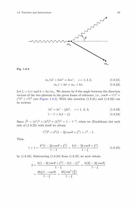
1.8 Particles and Interactions 89
Fig. 1.8.3
meγui + hνei = hνei, i = 1, 2, 3, (1.8.21)meγ + hν = me + hν. (1.8.22)
Let ξ = ν/ν and k = hν/me. We denote by θ the angle between the directionvectors of the two photons in the given frame of reference, i.e., cos θ = e1e1 +e2e2 + e3e3 (see Figure 1.8.3). With this notation (1.8.21) and (1.8.22) canbe written
γui = kei − ξkei, i = 1, 2, 3, (1.8.23)γ − 1 = k(1 − ξ). (1.8.24)
Since β2 = (u1)2 + (u2)2 + (u3)2 = 1 − γ−2, when we (Euclidean) dot eachside of (1.8.23) with itself we obtain
γ2β2 = k2(1 − 2ξ cos θ + ξ2) = γ2 − 1.
Thus,
γ + 1 =k2(1 − 2ξ cos θ + ξ2)
γ − 1=
k(1 − 2ξ cos θ + ξ2)1 − ξ
(1.8.25)
by (1.8.24). Subtracting (1.8.24) from (1.8.25) we next obtain
2 =k(1 − 2ξ cos θ + ξ2) − k(1 − ξ)2
1 − ξ=
k(2ξ − 2ξ cos θ)1 − ξ
=2kξ(1 − cos θ)
1 − ξ=
4kξ sin2(
θ2
)1 − ξ
.
90 1 Geometrical Structure of M
Thus, 2kξ sin2(
θ2
)= 1−ξ and therefore ξ = 1
1+2k sin2(θ/2)so ν = ν
1+2k sin2(θ/2).
From this we compute
λ − λ =1ν− 1
ν=
1 + 2k sin2(
θ2
)ν
− 1ν
=2k sin2
(θ2
)ν
.
We conclude that
λ − λ =2h
mesin2(
θ2
)(1.8.26)
which gives the change in wavelength of the photon as a function of the angleθ through which it is deflected (in the frame in which the electron is initiallyat rest). Observe that this change in wavelength does not depend on thewavelength λ of the incident photon, but only on the angle through whichit is deflected. Moreover, this difference ranges from a minimum of 0 whenθ = 0 (the photon and electron do not interact physically) to a maximum of
Δλmax =2h
me(1.8.27)
when θ = π (the photon is thrown straight back). This maximum change inwavelength is a characteristic feature of the electron; the quantity h/me iscalled the Compton wavelength of the electron.
Next we consider an inelastic collision between two material particles.The situation we have in mind is as follows: two free material particles withmasses m1 and m2 collide and coalesce to form a third material particle ofmass m3. Classically it is assumed that m3 = m1+m2 and on the basis of thisassumption (and the conservation of Newtonian momentum) one finds thatkinetic energy is lost during the collision. In Newtonian mechanics this lostkinetic energy disappears entirely from the mechanical picture in the sensethat it is viewed as having taken the form of heat in the combined particle andtherefore cannot be discussed further by the methods of mechanics. We shallsee that this rather unsatisfactory feature of Newtonian mechanics is avoidedin relativistic mechanics by observing that conservation of world momentum(which includes the conservation of energy) requires that the “hot” combinedparticle have a proper mass which is greater than the sum of the two massesfrom which it is formed, the difference m3 − (m1 + m2) being a measure ofthe energy required to bind the two particles together; this energy “acts likemass” in the combined particle.
We shall therefore consider a contact interaction (A, x, A), where A con-sists of two free material particles with proper masses m1 and m2 and worldvelocities U1 and U2 respectively and A consists of one free material particlewith proper mass m3 and world velocity U3. Conservation of world momen-tum requires that
m3U3 = m1U1 + m2U2. (1.8.28)

1.8 Particles and Interactions 91
Again observe that the Reversed Triangle Inequality (Theorem 1.4.2) givesm3 > m1 + m2. Moreover, since U1 · U1 = U2 · U2 = U3 · U3 = −1 we obtain(by dotting both sides of (1.8.28) with itself and using any admissible frameof reference)
m23 = m2
1 + m22 − 2m1m2U1 · U2,
m23 = m2
1 + m22 − 2m1m2γ1γ2(
⇀u 1, 1) · (⇀
u 2, 1), (1.8.29)
m23 = m2
1 + m22 + 2m1m2γ1γ2(1 − ⇀
u1 ·⇀u 2),
which yields the resultant mass m3 in terms of m1, m2 and the quantities ui1
and ui2, i = 1, 2, 3, which can be measured in the given frame of reference.
From (1.8.28) one can then compute U3.We wish to obtain an approximate formula for m3 which can be compared
with the Newtonian expression for the loss in kinetic energy. Assume that β1
and β2 are small so that γ1 and γ2 are approximately 1 (the frame of referenceis then no longer arbitrary, of course). We will eventually take γ1γ2 ≈ 1, butfirst we consider the somewhat better approximations
γj ≈ 1 + 12β2
j , j = 1, 2,
obtained from the binomial expansion (1.8.2). Then
γ1γ2 ≈(1 + 1
2β2
1
) (1 + 1
2β2
2
)= 1 + 1
2β2
1 + 12β2
2 + 14β2
1β22 ,
γ1γ2 ≈ 1 + 12β2
1 + 12β2
2 . (1.8.30)
Exercise 1.8.8 Show that (1.8.29) and (1.8.30) yield
m23 ≈ (m1 + m2)2 + m1m2
(β2
1 + β22 − 2γ1γ2(
⇀u 1 ·
⇀u 2)). (1.8.31)
Now taking γ1γ2 ≈ 1 in (1.8.31) we obtain
m23 ≈ (m1 + m2)2 + m1m2|
⇀v |2, (1.8.32)
where |⇀v |2 is the squared magnitude of the relative velocity⇀v =
⇀u1 − ⇀
u 2
of the two particles in A as measured in the given frame. From (1.8.32) weobtain
m3 ≈ m1 + m2 +m1m2
m1 + m2 + m3|⇀v |2.
Assuming that m3 ≈ m1 + m2 in the denominator we arrive at
m3 ≈ m1 + m2 + 12
m1m2
m1 + m2|⇀v |2, (1.8.33)
where the last term represents the approximate gain in proper mass as aresult of the collision.
92 1 Geometrical Structure of M
Now, in Newtonian mechanics it is assumed that m3 = m1 + m2 so thatconservation of Newtonian momentum requires that
(m1 + m2)⇀u3 = m1
⇀u1 + m2
⇀u2. (1.8.34)
Taking the Euclidean dot product of each side of (1.8.34) with itself thenyields
(m1 + m2)2|⇀u3|2 = m2
1|⇀u 1|2 + m2
2|⇀u2|2 + 2m1m2(
⇀u 1 ·
⇀u2). (1.8.35)
Exercise 1.8.9 Use (1.8.35) to show that the classical loss in kinetic energydue to the collision is given by
12m1|
⇀u 1|2 +
12m2|
⇀u 2|2 −
12(m1 + m2)|
⇀u3|2 =
12
m1m2
m1 + m2|⇀v |2,
where |⇀v |2 = |⇀u 1 −⇀u2|2.
Consequently, the Newtonian expression for the lost kinetic energy coincideswith the relativistic formula (1.8.33) for the approximate gain in proper massof the combined particle.

Chapter 2
Skew-Symmetric LinearTransformations andElectromagnetic Fields
2.1 Motivation via the Lorentz Law
A charged particle in M is a triple (α, m, e), where (α, m) is a materialparticle and e is a nonzero real number called the charge of the particle.A free charged particle is a charged particle (α, m, e), where (α, m) is a freematerial particle. Charged particles do two things of interest to us. By theirvery presence they create electromagnetic fields and they also respond to thefields created by other charges. Our objective in this chapter is to isolate theappropriate mathematical object with which to model an electromagneticfield in M, derive many of its basic properties and then investigate these twoactivities.
Charged particles “respond” to the presence of an electromagnetic fieldby experiencing changes in world momentum. The quantitative nature ofthis response is expressed by a differential equation relating the proper timederivative of the particle’s world momentum to the field. This equation ofmotion is generally taken to be the so-called Lorentz World Force Law (orLorentz 4-Force Law) which expresses the rate at which the particle’s worldmomentum changes at each point on the worldline as a linear function of theparticle’s world velocity:
dPdτ
= eFU , (2.1.1)
where U = U(τ) is the particle’s world velocity, P = mU its world momentumand, at each point, F : M → M is a linear transformation defined in terms ofthe classical “electric and magnetic 3-vectors
⇀
E and⇀
B” at that point ((2.1.1)is an abbreviated version of the somewhat more accurate and considerablymore cumbersome dP(τ)
dτ = eFα(τ)(U(τ)), where Fα(τ) is the appropriatelinear transformation at α(τ) ∈ M). We should point out that (2.1.1) canbe regarded as an appropriate equation of motion for charged particles in an
, : An Introduction , Applied Mathematical Sciences 92,
G.L. Naber The Geometry of Minkowski Spacetime to the Mathematics of the Special Theory of RelativityDOI 10.1007/978-1-4419-7838-7_2, © Springer Science+Business Media, LLC 2012
93
94 2 Skew-Symmetric Linear Transformations and Electromagnetic Fields
electromagnetic field only if the charges whose motion is to be governed by ithave negligible contribution to the ambient field. It must be possible to regardthe field as “given” and the charged particles as “test charges”. The muchmore difficult question of the interactions between the given field and thefields created by the moving charges will not be considered here (see [Par]).
We argue now that the form of the Lorentz Law (2.1.1) suggests that thelinear transformations F must be of a particular type (“skew-symmetric”).Indeed, rewriting (2.1.1) at each fixed point of M as
FU =m
e
dUdτ
and dotting both sides with U gives
FU · U =m
e
dUdτ
· U =m
eA · U = 0
since a material particle’s world velocity and world acceleration are alwaysorthogonal (Exercise 1.4.12). Since any unit timelike vector u ∈ M is theworld velocity of some charged particle (construct one!) we find that, for anysuch u, Fu ·u = 0. Linearity therefore implies that Fv · v = 0 for all timelike v.Now, if u and v are timelike and future-directed, then u + v is also timelikeand so 0 = F (u + v) · (u + v) = (Fu + Fv) · (u + v) = Fu · v + Fv ·u = Fu · v +u ·Fv . Thus, Fu · v = −u · Fv . But M has a basis of future-directed timelikevectors so it follows that F must satisfy
Fx · y = −x · Fy (2.1.2)
for all x and y in M. A linear transformation F : M → M which satisfies(2.1.2) for all x and y in M is said to be skew-symmetric (with respect tothe Lorentz inner product on M).
At each fixed point in M we therefore elect to model an electromagneticfield by a skew-symmetric linear transformation F whose job it is to assignto the world velocity U of a charged particle passing through that pointthe change in world momentum dP
dτ= eFU that the particle should expect
to experience due to the field. One would picture the electromagnetic fieldin toto therefore as a smooth assignment of such a linear transformationto each point in (some region of) M (although we shall find that natureimposes a condition—Maxwell’s Equations—on the manner in which such anassignment can be made). In the next four sections we carry out a generalinvestigation of skew-symmetric linear transformations on M and then turnto some physical applications in the last two sections.
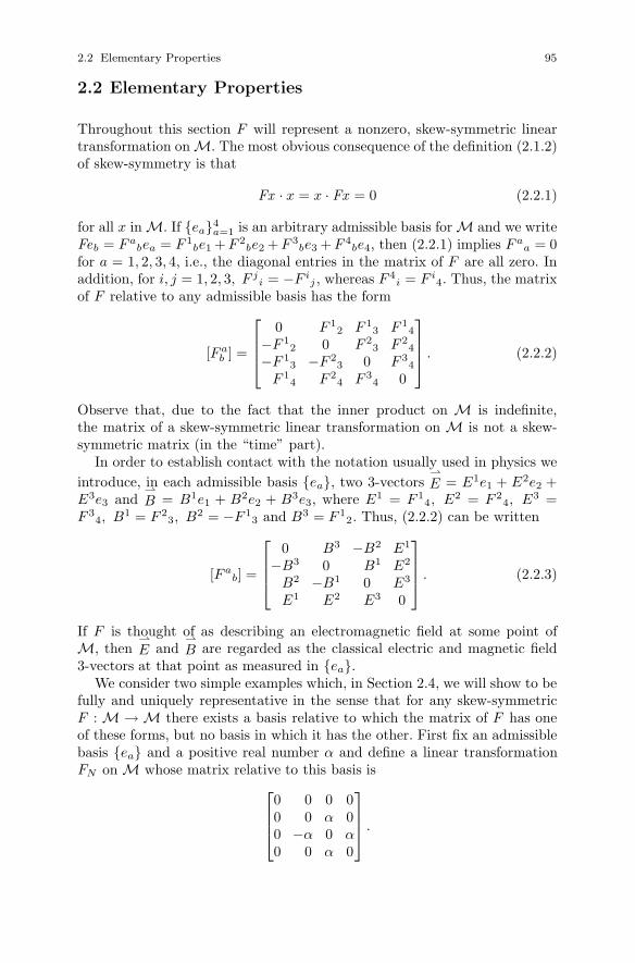
2.2 Elementary Properties 95
2.2 Elementary Properties
Throughout this section F will represent a nonzero, skew-symmetric lineartransformation on M. The most obvious consequence of the definition (2.1.2)of skew-symmetry is that
Fx · x = x · Fx = 0 (2.2.1)
for all x in M. If {ea}4a=1 is an arbitrary admissible basis for M and we write
Feb = F abea = F 1
be1 + F 2be2 + F 3
be3 + F 4be4, then (2.2.1) implies F a
a = 0for a = 1, 2, 3, 4, i.e., the diagonal entries in the matrix of F are all zero. Inaddition, for i, j = 1, 2, 3, F j
i = −F ij , whereas F 4
i = F i4. Thus, the matrix
of F relative to any admissible basis has the form
[F ab ] =
⎡⎢⎢⎣0 F 1
2 F 13 F 1
4
−F 12 0 F 2
3 F 24
−F 13 −F 2
3 0 F 34
F 14 F 2
4 F 34 0
⎤⎥⎥⎦ . (2.2.2)
Observe that, due to the fact that the inner product on M is indefinite,the matrix of a skew-symmetric linear transformation on M is not a skew-symmetric matrix (in the “time” part).
In order to establish contact with the notation usually used in physics weintroduce, in each admissible basis {ea}, two 3-vectors
⇀
E = E1e1 + E2e2 +E3e3 and
⇀
B = B1e1 + B2e2 + B3e3, where E1 = F 14, E2 = F 2
4, E3 =F 3
4, B1 = F 23, B2 = −F 1
3 and B3 = F 12. Thus, (2.2.2) can be written
[F ab] =
⎡⎢⎢⎣0 B3 −B2 E1
−B3 0 B1 E2
B2 −B1 0 E3
E1 E2 E3 0
⎤⎥⎥⎦ . (2.2.3)
If F is thought of as describing an electromagnetic field at some point ofM, then
⇀E and
⇀B are regarded as the classical electric and magnetic field
3-vectors at that point as measured in {ea}.We consider two simple examples which, in Section 2.4, we will show to be
fully and uniquely representative in the sense that for any skew-symmetricF : M → M there exists a basis relative to which the matrix of F has oneof these forms, but no basis in which it has the other. First fix an admissiblebasis {ea} and a positive real number α and define a linear transformationFN on M whose matrix relative to this basis is⎡⎢⎢⎣
0 0 0 00 0 α 00 −α 0 α0 0 α 0
⎤⎥⎥⎦ .
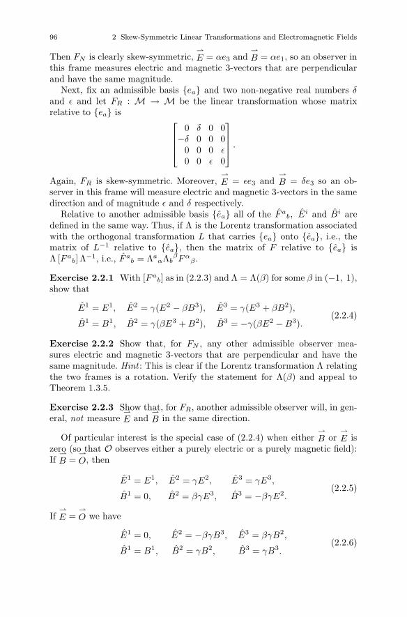
96 2 Skew-Symmetric Linear Transformations and Electromagnetic Fields
Then FN is clearly skew-symmetric,⇀
E = αe3 and⇀
B = αe1, so an observer inthis frame measures electric and magnetic 3-vectors that are perpendicularand have the same magnitude.
Next, fix an admissible basis {ea} and two non-negative real numbers δand ε and let FR : M → M be the linear transformation whose matrixrelative to {ea} is ⎡⎢⎢⎣
0 δ 0 0−δ 0 0 0
0 0 0 ε0 0 ε 0
⎤⎥⎥⎦ .
Again, FR is skew-symmetric. Moreover,⇀
E = εe3 and⇀
B = δe3 so an ob-server in this frame will measure electric and magnetic 3-vectors in the samedirection and of magnitude ε and δ respectively.
Relative to another admissible basis {ea} all of the F ab, Ei and Bi are
defined in the same way. Thus, if Λ is the Lorentz transformation associatedwith the orthogonal transformation L that carries {ea} onto {ea}, i.e., thematrix of L−1 relative to {ea}, then the matrix of F relative to {ea} isΛ [F a
b] Λ−1, i.e., F ab = Λa
αΛbβFα
β.
Exercise 2.2.1 With [F ab] as in (2.2.3) and Λ = Λ(β) for some β in (−1, 1),
show that
E1 = E1, E2 = γ(E2 − βB3), E3 = γ(E3 + βB2),
B1 = B1, B2 = γ(βE3 + B2), B3 = −γ(βE2 − B3).(2.2.4)
Exercise 2.2.2 Show that, for FN , any other admissible observer mea-sures electric and magnetic 3-vectors that are perpendicular and have thesame magnitude. Hint : This is clear if the Lorentz transformation Λ relatingthe two frames is a rotation. Verify the statement for Λ(β) and appeal toTheorem 1.3.5.
Exercise 2.2.3 Show that, for FR, another admissible observer will, in gen-eral, not measure
⇀E and
⇀B in the same direction.
Of particular interest is the special case of (2.2.4) when either⇀
B or⇀
E iszero (so that O observes either a purely electric or a purely magnetic field):If
⇀
B =⇀
O, then
E1 = E1, E2 = γE2, E3 = γE3,
B1 = 0, B2 = βγE3, B3 = −βγE2.(2.2.5)
If⇀
E =⇀
O we have
E1 = 0, E2 = −βγB3, E3 = βγB2,
B1 = B1, B2 = γB2, B3 = γB3.(2.2.6)
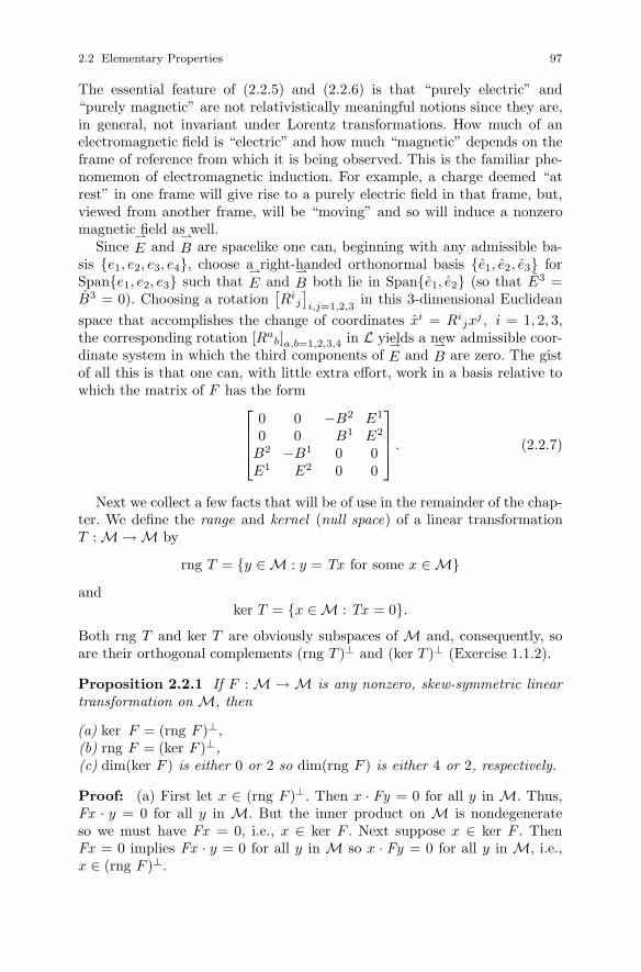
2.2 Elementary Properties 97
The essential feature of (2.2.5) and (2.2.6) is that “purely electric” and“purely magnetic” are not relativistically meaningful notions since they are,in general, not invariant under Lorentz transformations. How much of anelectromagnetic field is “electric” and how much “magnetic” depends on theframe of reference from which it is being observed. This is the familiar phe-nomemon of electromagnetic induction. For example, a charge deemed “atrest” in one frame will give rise to a purely electric field in that frame, but,viewed from another frame, will be “moving” and so will induce a nonzeromagnetic field as well.
Since⇀
E and⇀
B are spacelike one can, beginning with any admissible ba-sis {e1, e2, e3, e4}, choose a right-handed orthonormal basis {e1, e2, e3} forSpan{e1, e2, e3} such that
⇀
E and⇀
B both lie in Span{e1, e2} (so that E3 =B3 = 0). Choosing a rotation
[Ri
j
]i,j=1,2,3
in this 3-dimensional Euclideanspace that accomplishes the change of coordinates xi = Ri
jxj , i = 1, 2, 3,
the corresponding rotation [Rab]a,b=1,2,3,4 in L yields a new admissible coor-
dinate system in which the third components of⇀
E and⇀
B are zero. The gistof all this is that one can, with little extra effort, work in a basis relative towhich the matrix of F has the form⎡⎢⎢⎣
0 0 −B2 E1
0 0 B1 E2
B2 −B1 0 0E1 E2 0 0
⎤⎥⎥⎦ . (2.2.7)
Next we collect a few facts that will be of use in the remainder of the chap-ter. We define the range and kernel (null space) of a linear transformationT : M → M by
rng T = {y ∈ M : y = Tx for some x ∈ M}
andker T = {x ∈ M : Tx = 0}.
Both rng T and ker T are obviously subspaces of M and, consequently, soare their orthogonal complements (rng T )⊥ and (ker T )⊥ (Exercise 1.1.2).
Proposition 2.2.1 If F : M → M is any nonzero, skew-symmetric lineartransformation on M, then
(a) ker F = (rng F )⊥,(b) rng F = (ker F )⊥,(c) dim(ker F ) is either 0 or 2 so dim(rng F ) is either 4 or 2, respectively.
Proof: (a) First let x ∈ (rng F )⊥. Then x · Fy = 0 for all y in M. Thus,Fx · y = 0 for all y in M. But the inner product on M is nondegenerateso we must have Fx = 0, i.e., x ∈ ker F . Next suppose x ∈ ker F . ThenFx = 0 implies Fx · y = 0 for all y in M so x · Fy = 0 for all y in M, i.e.,x ∈ (rng F )⊥.

98 2 Skew-Symmetric Linear Transformations and Electromagnetic Fields
Exercise 2.2.4 Show that, for any subspace U of M, (U⊥)⊥ = U andconclude from (a) that (b) is true. Hint : Use the fact that U and U⊥ havecomplementary dimensions, i.e., dimU + dimU⊥ = dimM (see Theorem 16,Chapter 4 of [La]).
(c) Without loss of generality select a basis {ea} relative to which the matrixof F has the form (2.2.7). Then, for any v ∈ M, Fv has components given by⎡⎢⎢⎣
0 0 −B2 E1
0 0 B1 E2
B2 −B1 0 0E1 E2 0 0
⎤⎥⎥⎦⎡⎢⎢⎣
v1
v2
v3
v4
⎤⎥⎥⎦ =
⎡⎢⎢⎣−B2v3 + E1v4
B1v3 + E2v4
B2v1 − B1v2
E1v1 + E2v2
⎤⎥⎥⎦which is zero if and only if{
−B2v3 + E1v4 = 0,B1v3 + E2v4 = 0 and
{B2v1 − B1v2 = 0,E1v1 + E2v2 = 0.
Notice that the determinant of the coefficient matrix in the first system is−
⇀
E ·⇀
B and, in the second,⇀
E ·⇀
B. If⇀
E ·⇀
B �= 0 both systems have only thetrivial solution so the kernel of F consists of 0 alone and dim(ker F ) = 0. Since4 = dim M = dim(ker F ) + dim(rng F ), dim(rng F ) = 4. If
⇀
E ·⇀
B = 0, eachsystem has nontrivial solutions, say, (v3, v4) =
(v30, v
40
)and (v1,v2) =
(v10, v
20
).
Since F �= 0, all of the nontrivial solutions to the first system are of the formb(v30 , v
40
), b ∈ R, and, for the second, a(v1
0, v20), a ∈ R. Thus, the kernel of
F is the set of ⎡⎢⎢⎣v1
v2
v3
v4
⎤⎥⎥⎦ = a
⎡⎢⎢⎣v10
v20
00
⎤⎥⎥⎦+ b
⎡⎢⎢⎣00v30
v40
⎤⎥⎥⎦ ,
so dim(ker F ) = 2 and therefore dim(rng F ) = 2. �
Recall that a real number λ is an eigenvalue of F if there exists a nonzerox ∈ M such that Fx = λx and that any such x is an eigenvector of Fcorresponding to λ. The eigenspace of F corresponding to λ is {x ∈ M :Fx = λx}, i.e., the set of eigenvectors for λ together with 0 ∈ M, and it isindeed a subspace of M. A subspace U of M is said to be invariant under Fif F maps U into U , i.e., if FU ⊆ U . Any eigenspace of F is invariant underF since Fx = λx implies F (Fx ) = F (λx) = λFx .
Proposition 2.2.2 If F : M → M is any nonzero, skew-symmetric lineartransformation on M, then
(a) Fx = λx implies that either λ = 0 or x is null (or both),(b) FU ⊆ U implies F (U⊥) ⊆ U⊥.
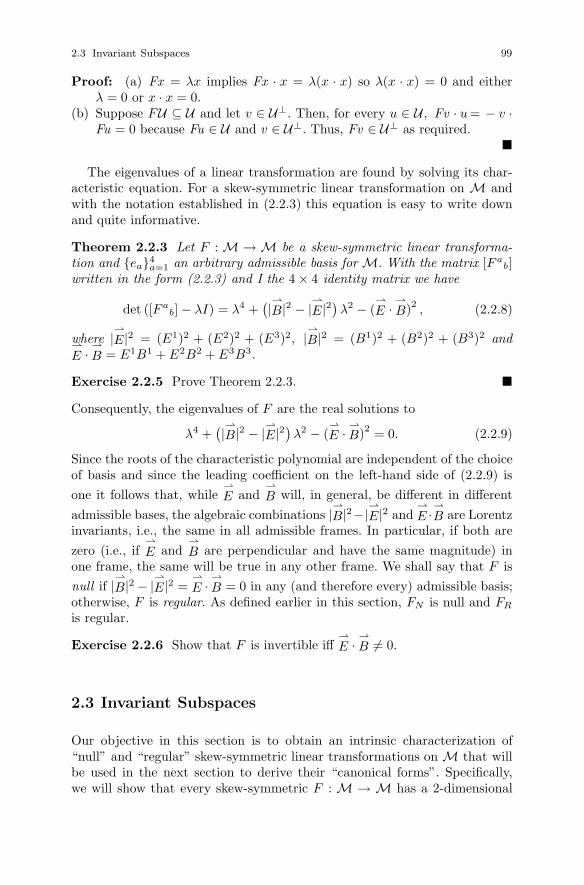
2.3 Invariant Subspaces 99
Proof: (a) Fx = λx implies Fx · x = λ(x · x) so λ(x · x) = 0 and eitherλ = 0 or x · x = 0.
(b) Suppose FU ⊆ U and let v ∈ U⊥. Then, for every u ∈ U , Fv · u = − v ·Fu = 0 because Fu ∈ U and v ∈ U⊥. Thus, Fv ∈ U⊥ as required.
�
The eigenvalues of a linear transformation are found by solving its char-acteristic equation. For a skew-symmetric linear transformation on M andwith the notation established in (2.2.3) this equation is easy to write downand quite informative.
Theorem 2.2.3 Let F : M → M be a skew-symmetric linear transforma-tion and {ea}4
a=1 an arbitrary admissible basis for M. With the matrix [F ab]
written in the form (2.2.3) and I the 4 × 4 identity matrix we have
det ([F ab] − λI) = λ4 +
(|⇀B|2 − |
⇀E|2)λ2 − (
⇀E ·
⇀B)2 , (2.2.8)
where |⇀
E|2 = (E1)2 + (E2)2 + (E3)2, |⇀
B|2 = (B1)2 + (B2)2 + (B3)2 and⇀
E ·⇀
B = E1B1 + E2B2 + E3B3.
Exercise 2.2.5 Prove Theorem 2.2.3. �
Consequently, the eigenvalues of F are the real solutions to
λ4 +(|⇀B|2 − |
⇀E|2)λ2 − (
⇀E ·
⇀B)2 = 0. (2.2.9)
Since the roots of the characteristic polynomial are independent of the choiceof basis and since the leading coefficient on the left-hand side of (2.2.9) isone it follows that, while
⇀
E and⇀
B will, in general, be different in differentadmissible bases, the algebraic combinations |
⇀
B|2−|⇀
E|2 and⇀
E ·⇀
B are Lorentzinvariants, i.e., the same in all admissible frames. In particular, if both arezero (i.e., if
⇀
E and⇀
B are perpendicular and have the same magnitude) inone frame, the same will be true in any other frame. We shall say that F isnull if |
⇀
B|2 − |⇀
E|2 =⇀
E ·⇀
B = 0 in any (and therefore every) admissible basis;otherwise, F is regular. As defined earlier in this section, FN is null and FR
is regular.
Exercise 2.2.6 Show that F is invertible iff⇀
E ·⇀
B �= 0.
2.3 Invariant Subspaces
Our objective in this section is to obtain an intrinsic characterization of“null” and “regular” skew-symmetric linear transformations on M that willbe used in the next section to derive their “canonical forms”. Specifically,we will show that every skew-symmetric F : M → M has a 2-dimensional
100 2 Skew-Symmetric Linear Transformations and Electromagnetic Fields
invariant subspace and that F is regular if and only if U ∩ U⊥ = {0} forsome such subspace U (so F is null if and only if U ∩ U⊥ �= {0} for every2-dimensional invariant subspace U).
We begin with a few observations on invariant subspaces in general. Let Vbe a real vector space of dimension at least 2 and T : V → V a nonzero lineartransformation. Observe that if the characteristic equation det(T − λI) = 0has a real root λ, then T has an eigenvector, i.e., there is a nonzero v ∈ Vsuch that Tv = λv. Consequently, Span{v} is a non-trivial invariant subspacefor T . If there are no real roots the situation is less simple.
Lemma 2.3.1 Let V be a real vector space of dimension greater than orequal to 2 and T : V → V a nonzero linear transformation. If det(T −λI) = 0has a complex solution λ = α + βi, β �= 0, then there exist nonzero vectors xand y in V such that
Tx = αx − βy and Ty = αy + βx. (2.3.1)
In particular, Span{x, y} is a nontrivial invariant subspace for T .
Proof: Select a basis for V and let [aij ]i,j=1,...,n be the matrix of T in thisbasis. Since det(T − λI) = 0 when λ = α + βi, the system⎧⎪⎨⎪⎩
a11z1 + · · · + a1nzn = (α + βi)z1
......
...an1z1 + · · · + annzn = (α + βi)zn
as a nontrivial complex solution z1 = x1 + iy1, . . . , zn = xn + iyn. Thus,⎧⎪⎨⎪⎩a11(x1 + iy1) + · · · + a1n(xn + iyn) = (α + βi)(x1 + iy1)
......
...an1(x1 + iy1) + · · · + ann(xn + iyn) = (α + βi)(xn + iyn) .
Separating into real and imaginary parts gives⎧⎪⎨⎪⎩a11x1 + · · · + a1nxn = αx1 − βy1
......
...an1x1 + · · · + annxn = αxn − βyn
(2.3.2)
and ⎧⎪⎨⎪⎩a11y1 + · · · + a1nyn = αy1 + βx1
......
...an1y1 + · · · + annyn = αyn + βxn.
(2.3.3)
Let x and y be the vectors in V whose components relative to our basis arex1, . . . , xn and y1, . . . , yn respectively. Then Tx = αx−βy and Ty = αy+βxas required. Notice that neither x nor y is zero since if x = 0, (2.3.2) and the

2.3 Invariant Subspaces 101
fact that β �= 0 imply y = 0 so z1 = · · · = zn = 0, which is a contradiction.Similarly, y = 0 implies x = 0 so, in fact, neither can be zero. �
In order to apply this result to the case of interest to us we require two finalpreliminary results.
Lemma 2.3.2 Let A and B be real numbers with B �= 0. Then the equationλ4 + Aλ2 − B2 = 0 has a complex solution.
Proof: Regard λ4 + Aλ2 − B2 = 0 as a quadratic in λ2 to obtain λ2 =12 (−A±
√A2 + 4B2). Choosing the minus sign gives a negative λ2 and there-
fore complex λ. �
Lemma 2.3.3 Let F : M → M be a nonzero, skew-symmetric linear trans-formation. If the characteristic equation
λ4 + (|⇀
B|2 − |⇀
E|2)λ2 − (⇀
E ·⇀
B)2 = 0
has two distinct nonzero, real solutions, then there exists a 2-dimensionalsubspace U of M which is invariant under F and satisfies U ∩ U⊥ = {0}.
Proof: Let λ1 and λ2 be the two distinct nonzero real eigenvalues. Thenthere exist nonzero vectors x and y such that Fx = λ1x and Fy = λ2y. ByProposition 2.2.2(a), x and y are null. Observe next that x and y are linearlyindependent. Indeed, ax + by = 0 implies
aFx + bFy = 0,
a(λ1x) + b(λ2y) = 0,
λ1(ax ) + λ2(by) = 0,
λ1(ax ) + λ2(−ax ) = 0,
(λ1 − λ2)ax = 0.
Since λ1 − λ2 �= 0, ax = 0, but x is nonzero so a = 0. Similarly, b = 0 so xand y are independent. Thus, U = Span{x, y} is 2-dimensional; it is clearlyinvariant under F . Now suppose ax + by ∈ U ∩ U⊥. Then, in particular,
(ax + by) · x = 0,
a(x · x) + b(x · y) = 0,
b(x · y) = 0.
But x and y are null and nonparallel so x · y �= 0 and therefore b = 0.Similarly, a = 0 so U ∩ U⊥ = {0}. �
Theorem 2.3.4 Let F : M → M be a nonzero, skew-symmetric lineartransformation on M. If F is regular, then there exists a 2-dimensional sub-space U of M which is invariant under F and satisfies U ∩ U⊥ = {0}.

102 2 Skew-Symmetric Linear Transformations and Electromagnetic Fields
Proof: Relative to any admissible basis, at least one of⇀
E ·⇀
B or |⇀
B|2 − |⇀
E|2must be nonzero and F ’s characteristic equation is
λ4 + (|⇀
B|2 − |⇀
E|2)λ2 − (⇀
E ·⇀
B)2 = 0. (2.3.4)
We consider four cases:
1.⇀
E ·⇀
B = 0 and |⇀
B|2 − |⇀
E|2 < 0.
In this case (2.3.4) becomes λ2(λ2 + (|⇀
B|2 − |⇀
E|2)) = 0 and the solutions
are λ = 0 and λ = ±√|⇀
E|2 − |⇀
B|2. The latter are two distinct, nonzero realsolutions so Lemma 2.3.3 yields the result.
2.⇀
E ·⇀
B = 0 and |⇀
B|2 − |⇀
E|2 > 0.
The solutions of (2.3.4) are now λ = 0 and λ = ±βi, where β =√|⇀
B|2 − |⇀
E|2.Lemma 2.3.1 implies that there exist nonzero vectors x and y in M such that
Fx = −βy and Fy = βx. (2.3.5)
We claim that x and y are linearly independent. Indeed, suppose ax +by = 0with, say, b �= 0. Then y = kx , where k = −a/b. Then Fx = −βy impliesFx = (−βk)x. But F ’s only real eigenvalue is 0 and β �= 0 so k = 0 andtherefore y = 0, which is a contradiction. Thus, b = 0. Since x �= 0, ax = 0implies a = 0 and the proof is complete.
Thus, U = Span{x, y} is a 2-dimensional subspace of M that is invariantunder F . We claim that U ∩ U⊥ = {0}. Suppose ax + by ∈ U ∩ U⊥.
Then ax + by is null so (ax + by) · (ax + by) = 0, i.e.,
a2(x · x) + 2ab(x · y) + b2(y · y) = 0.
But x · y = x · (− 1β Fx) = − 1
β (x · Fx ) = 0 so
a2(x · x) + b2(y · y) = 0,
a2x ·(
1β
Fy)
+ b2y ·(− 1
βFx)
= 0,(a2
β
)x · Fy −
(b2
β
)y · Fx = 0,(
a2
β
)x · Fy +
(b2
β
)x · Fy = 0,(
a2 + b2
β
)x · Fy = 0.
Now, if a2 + b2 �= 0, then x · Fy = 0 so x · (βx) = 0 and x · x = 0. Similarly,y · y = 0 so x and y are orthogonal null vectors and consequently parallel.But this is a contradiction since x and y are independent. Thus, a2 + b2 = 0so a = b = 0 and U ∩ U⊥ = {0}.

2.3 Invariant Subspaces 103
3.⇀
E ·⇀
B �= 0 and |⇀
B|2 − |⇀
E|2 = 0.
In this case (2.3.4) becomes λ4 = (⇀
E ·⇀
B)2 so λ2 = ±|⇀
E ·⇀
B|. λ2 = |⇀
E ·⇀
B|gives two distinct, nonzero real solutions so the conclusion follows fromLemma 2.3.3.
4.⇀
E ·⇀
B �= 0 and |⇀
B|2 − |⇀
E|2 �= 0.
Lemma 2.3.2 implies that (2.3.4) has a complex root α + βi(β �= 0). Thus,Lemma 2.3.1 yields nonzero vectors x and y in M with
Fx = αx − βy and Fy = αy + βx.
There are two possibilities:
i. x and y are linearly dependent. Then, since neither is zero, y = kx forsome k ∈ R with k �= 0. Thus, Fx = αx−βy = αx−kβx = (α−kβ)x andFy = αy + βx = αy + β
k y =(α + β
k
)y. Since α + β
k �= α − kβ and since0 is not a solution to (2.3.4) in this case we find that F has two distinct,nonzero real eigenvalues and again appeal to Lemma 2.3.3.
ii. x and y are linearly independent. Then U = Span{x, y} is a 2-dimensionalsubspace of M that is invariant under F .
Exercise 2.3.1 Complete the proof by showing that U ∩ U⊥ = {0}. �
To complete our work in this section we must show that a nonzero nullskew-symmetric F : M → M has 2-dimensional invariant subspaces and thatall of these intersect their orthogonal complements nontrivially. We addressthe question of existence first.
Proposition 2.3.5 Let F : M → M be a nonzero, null, skew-symmetriclinear transformation on M. Then both ker F and rng F = (ker F )⊥
are 2-dimensional invariant subspaces of M and their intersection is a1-dimensional subspace of M spanned by a null vector.
Proof: ker F and rng F are obviously invariant under F . Since F is null,⇀
E ·⇀
B = 0 so, by Exercise 2.2.6, F is not invertible. Thus, dim(ker F ) �= 0.Proposition 2.2.1(c) then implies that dim(ker F ) = 2 and, consequently,dim(rng F ) = 2.
Now, since rng F ∩ ker F = rng F ∩ (rng F )⊥ by Proposition 2.2.1(a), ifthis intersection is not {0}, it can contain only null vectors. Being a subspaceof M it must therefore be 1-dimensional. We show that this intersectionis, indeed, nontrivial as follows: For a null F the characteristic polynomial(2.3.4) reduces to λ4 = 0. The Cayley-Hamilton Theorem (see [H]) thereforeimplies that
F 4 = 0 (F null). (2.3.6)
104 2 Skew-Symmetric Linear Transformations and Electromagnetic Fields
Next we claim that ker F � ker F 2. ker F ⊆ ker F 2 is obvious. Now, supposeker F = ker F 2, i.e., Fx = 0 iff F 2x = 0. Then
F 3x = F 2(Fx ) = 0 =⇒ Fx ∈ ker F 2 = ker F
=⇒ F (Fx ) = 0
=⇒ F 2x = 0=⇒ Fx = 0 by assumption,
so F 3x = 0 =⇒ Fx = 0 and we conclude that ker F 3 = ker F . Repeating theargument gives ker F 4 = ker F . But by (2.3.6), ker F 4 = M so ker F = Mand F is identically zero, contrary to hypothesis. Thus, ker F � ker F 2 andwe may select a nonzero v ∈ M such that F 2v = 0, but Fv �= 0. Thus,Fv ∈ rng F ∩ ker F as required. �
Exercise 2.3.2 Show that if F :M → M is a nonzero, null, skew-symmetriclinear transformation on M, then F 2v is null (perhaps 0) for every v ∈ M.Hint : Begin with (2.3.6).
All that remains is to show that if F is null, then every 2-dimensional invari-ant subspace U satisfies U ∩ U⊥ �= {0}.
Lemma 2.3.6 Let F : M → M be a nonzero, skew-symmetric linear trans-formation on M. If there exists a 2-dimensional invariant subspace U for Fwith U ∩ U⊥ = {0}, then U⊥ is also a 2-dimensional invariant subspace forF and there exists a real number α such that F 2u = αu for every u ∈ U .
Proof: U⊥ is a subspace of M (Exercise 1.1.2) and is invariant under F(Proposition 2.2.2(b)). Notice that the restriction of the Lorentz inner prod-uct to U cannot be degenerate since this would contradict U ∩ U⊥ = {0}.Thus, by Theorem 1.1.1, we may select an orthonormal basis {u1, u2} for U .Now, let x be an arbitrary element of M. If u1 and u2 are both spacelike,then v = x− [(x ·u1)u1 +(x ·u2)u2] ∈ U⊥ and x = v + [(x ·u1)u1 +(x ·u2)u2]so x ∈ U + U⊥.
Exercise 2.3.3 Argue similarly that if {u1, u2} contains one spacelike andone timelike vector, then any x ∈ M is in U + U⊥ and explain why this isthe only remaining possibility for the basis {u1, u2}.
Since U ∩ U⊥ = {0} we conclude that M = U⊕
U⊥ so dim U⊥ = 2.Now we let {u1, u2} be an orthonormal basis for U and write Fu1 = au1 +
bu2 and Fu2 = cu1 + du2. Then, since neither u1 nor u2 is null, we have0 = Fu1 · u1 = (au1 + bu2) · u1 = ±a so a = 0 and, similarly, d = 0.Thus, Fu1 = bu2 and Fu2 = cu1, so F 2u1 = F (bu2) = bFu2 = bcu1 andF 2u2 = bcu2. Let α = bc. Then, for any u = βu1 + γu2 ∈ U we haveF 2u = βF 2u1 +γF 2u2 = β(αu1)+γ(αu2) = α(βu1 +γu2) = αu as required.
�

2.4 Canonical Forms 105
With this we can show that if F is null and nonzero and U is a 2-dimensional invariant subspace for F , then U ∩ U⊥ �= {0}. Suppose, to thecontrary, that U ∩U⊥ = {0}. Lemma 2.3.6 implies the existence of an α ∈ R
such that F 2u = αu for all u in U . Thus, F 4u = F 2(F 2u) = F 2(αu) =αF 2u = α2u for all u ∈ U . But, by (2.3.6), F 4u = 0 for all u ∈ U so α = 0and F 2 = 0 on U . Again by Lemma 2.3.6 we may apply the same argumentto U⊥ to obtain F 2 = 0 on U⊥. Since U and U⊥ are 2-dimensional andU ∩ U⊥ = {0}, M = U
⊕U⊥ so F 2 = 0 on all of M. But then, for every
u ∈ M, F 2u ·u = 0 so Fu ·Fu = 0, i.e., rng F contains only null vectors. Butthen dim(rng F ) = 1 and this contradicts Proposition 2.2.1(c) and we haveproved:
Theorem 2.3.7 Let F : M → M be a nonzero, skew-symmetric lineartransformation on M. If F is null, then F has 2-dimensional invariant sub-spaces and every such subspace U satisfies U ∩ U⊥ �= {0}.
Combining this with Theorem 2.3.4 gives:
Corollary 2.3.8 Let F : M → M be a nonzero, skew-symmetric lineartransformation on M. Then F has 2-dimensional invariant subspaces and Fis regular i f f there exists such a subspace U such that U ∩U⊥ = {0} (so F isnull i f f U ∩ U⊥ �= {0} for every such subspace).
2.4 Canonical Forms
We now propose to use the results of the preceding section to prove that, forany skew-symmetric linear transformation F : M → M, there exists a basisfor M relative to which the matrix of F has one of the two forms⎡⎢⎢⎣
0 δ 0 0−δ 0 0 0
0 0 0 ε0 0 ε 0
⎤⎥⎥⎦ or
⎡⎢⎢⎣0 0 0 00 0 α 00 −α 0 α0 0 α 0
⎤⎥⎥⎦ ,
depending on whether F is regular or null respectively. We begin with theregular case.
Thus, we suppose F : M → M is a nonzero, skew-symmetric linear trans-formation and that (Corollary 2.3.8) there exists a 2-dimensional subspace Uof M which satisfies FU ⊆ U and U ∩ U⊥ = {0}. Then (Lemma 2.3.6) U⊥ isalso a 2-dimensional invariant subspace for F and there exist real numbers αand β such that
F 2u = αu for all u ∈ U and (2.4.1)
F 2v = βv for all v ∈ U⊥. (2.4.2)
106 2 Skew-Symmetric Linear Transformations and Electromagnetic Fields
Since M = U⊕
U⊥ and U⊥⊥ = U we may assume, without loss of generality,that the restriction of the Lorentz inner product to U has index 1 and itsrestriction to U⊥ has index 0.
We claim now that α ≥ 0 and β ≤ 0. Indeed, dotting both sides of (2.4.1)with itself gives F 2u ·u = α(u ·u), or −Fu ·Fu = α(u ·u) for any u in U . Nowif u ∈ U is timelike, then Fu is spacelike or zero so u · u < 0 and Fu · Fu ≥ 0and this implies α ≥ 0. Thus, we may write α = ε2 with ε ≥ 0 so (2.4.1)becomes
F 2u = ε2u for all u ∈ U . (2.4.3)
Exercise 2.4.1 Show that, for some δ ≥ 0,
F 2v = −δ2v for all v ∈ U⊥. (2.4.4)
Now, select a future-directed unit timelike vector e4 in U . Then Fe4 isspacelike or zero and in U so we may select a unit spacelike vector e3 in Uwith Fe4 = ke3 for some k ≥ 0. Observe that ε2e4 = F 2e4 = F (Fe4) =F (ke3) = kFe3. Thus,
kFe3 · e4 = ε2e4 · e4,
k(−e3 · Fe4) = ε2(−1),
k(e3 · (ke3)) = ε2,
k2e3 · e3 = ε2,
so k2 = ε2 and k = ε (since k ≥ 0 and ε ≥ 0). Thus, we have
Fe4 = εe3. (2.4.5)
Notice that {e3, e4} is an orthonormal basis for U .
Exercise 2.4.2 Show that, in addition,
Fe3 = εe4. (2.4.6)
Now, let e2 be an arbitrary unit spacelike vector in U⊥. Then Fe2 is space-like or zero and in U⊥ so we may select another unit spacelike vector e1 inU⊥ and orthogonal to e2 with Fe2 = ke1 for some k ≥ 0 (if e1 × e2 · e3 is −1rather than 1, then relabel e1 and e2).
Exercise 2.4.3 Show that k = δ.
Thus,Fe2 = δe1 (2.4.7)
and, as for (2.4.6),Fe1 = −δe2. (2.4.8)
2.4 Canonical Forms 107
Now, {e1, e2, e3, e4} is an orthonormal basis for M and any basis constructedin this way is called a canonical basis for F. From (2.4.5)–(2.4.8) we find thatthe matrix of F relative to such a basis is⎡⎢⎢⎣
0 δ 0 0−δ 0 0 0
0 0 0 ε0 0 ε 0
⎤⎥⎥⎦ . (2.4.9)
This is just the matrix of the FR defined in Section 2.2. In a canonical basisan observer measures electric and magnetic fields in the x3-direction and ofmagnitudes ε and δ respectively. We have shown that such a frame existsfor any regular F . Observe that |
⇀
B|2 − |⇀
E|2 = δ2 − ε2 and⇀
E ·⇀
B = δε.Since these two quantities are invariants, δ and ε can be calculated from theelectric and magnetic 3-vectors in any frame. The canonical form (2.4.9) ofF is particularly convenient for calculations. For example, the fourth powerof the matrix (2.4.9) is easily computed and found to be⎡⎢⎢⎣
δ4 0 0 00 δ4 0 00 0 ε4 00 0 0 ε4
⎤⎥⎥⎦ ,
so that, unlike the null case, F 4 �= 0. The eigenvalues of F are of some interestand are also easy to calculate since the characteristic equation (2.3.4) becomesλ4+(δ2−ε2)λ2−δ2ε2 = 0 i.e., (λ2−ε2)(λ2+δ2) = 0 whose only real solutionsare λ = ±ε. The eigenspace corresponding to λ = ε is obtained by solving⎡⎢⎢⎣
0 δ 0 0−δ 0 0 0
0 0 0 ε0 0 ε 0
⎤⎥⎥⎦⎡⎢⎢⎣
v1
v2
v3
v4
⎤⎥⎥⎦ =
⎡⎢⎢⎣εv1
εv2
εv3
εv4
⎤⎥⎥⎦ ,
i.e., ⎡⎢⎢⎣δv2
−δv1
εv4
εv3
⎤⎥⎥⎦ =
⎡⎢⎢⎣εv1
εv2
εv3
εv4
⎤⎥⎥⎦ .
If ε = 0 and δ �= 0, then v1 = v2 = 0, whereas v3 and v4 are arbitrary. Thus,the eigenspace is Span{e3, e4}. Similarly, if ε �= 0 and δ = 0, v1 = v2 = 0and v3 = v4 so the eigenspace is Span{e3 + e4}. If εδ �= 0, δv2 = εv1 and−δv1 = εv2 again imply v1 = v2 = 0; in addition, v3 = v4 so the eigenspaceis Span{e3 + e4}. In the first case the eigenspace contains two independentnull directions (those of e3 + e4 and e3 − e4), whereas in the last two cases,there is only one (e3 + e4). For λ = −ε, the result is obviously the same in

108 2 Skew-Symmetric Linear Transformations and Electromagnetic Fields
the first case, while in the second and third the eigenspace is spanned bye3 − e4. The null directions corresponding to e3 ± e4 are called the principalnull directions of F .
Now we turn to the case of a nonzero, null, skew-symmetric linear trans-formation F : M → M and construct an analogous “canonical basis”. Beginwith an arbitrary future-directed unit timelike vector e4 in M.
Exercise 2.4.4 Show that Fe4 is spacelike. Hint : Fe4 = 0 would implye4 ∈ (rng F )⊥.
Thus, we may select a unit spacelike vector e3 in M such that e3 · e4 = 0 and
Fe4 = αe3 (2.4.10)
for some α > 0. Observe that e3 = F(
1αe4
)∈ rng F . Next we claim that
Fe3 is a nonzero vector in rng F ∩ ker F . Fe3 �= 0 is clear since Fe3 = 0 =⇒e3 ∈ rng F ∩ker F , but e3 is spacelike and this contradicts Proposition 2.3.5.Fe3 ∈ rng F is obvious. Now, by Exercise 2.3.2, F 2e3 is either zero or null andnonzero. F 2e3 = 0 implies F (Fe3) = 0 so Fe3 ∈ ker F as required. Suppose,on the other hand, that F 2e3 is null and nonzero. Fe3 ·F 2e3 = 0 implies thatFe3 is not timelike. Fe3 ·e3 = 0 implies that Fe3 is not spacelike since then rngF would contain a null and two orthogonal spacelike vectors, contradictingProposition 2.3.5. Thus, Fe3 is null and nonzero. But then {e3,Fe3} is abasis for rng F and Fe3 is orthogonal to both so Fe3 ∈ (rng F )⊥ = ker F asrequired.
Now we wish to choose a unit spacelike vector e2 such that e2 · e4 = 0,e2 · e3 = 0 and Span{e2 + e4} = rng F ∩ ker F . To see how this is done selectany null vector N spanning rng F ∩ ker F such that N · e4 = −1. Then lete2 = N − e4. It follows that e2 · e2 = (N − e4) · (N − e4) = N ·N − 2N · e4 +e4 ·e4 = 0−2(−1)−1 = 1 so e2 is unit spacelike. Moreover, e2+e4 = N spansrng F ∩ ker F . Also, e2 · e4 = (N − e4) · e4 = N · e4 − e4 · e4 = −1− (−1) = 0.Finally, e2 + e4 ∈ (rng F )⊥ implies 0 = (e2 + e4) · e3 = e2 · e3 + e4 · e3 = e2 · e3
and the construction is complete. Now, there exists an α′ > 0 such thatFe3 = α′(e2 + e4). But α = e3 · (αe3) = e3 · Fe4 = −e4 · [α′(e2 + e4)] =−α′[e4 · e2 + e4 · e4] = −α′[0 − 1] = α′ so
Fe3 = α(e2 + e4). (2.4.11)
Next we compute Fe2 = F (N − e4) = FN − Fe4 = 0 − αe3 so
Fe2 = −αe3. (2.4.12)
Finally, we select a unit spacelike vector e1 which is orthogonal to e2, e3 ande4 and satisfies e1 × e2 · e3 = 1 to obtain an admissible basis {ea}4
a=1.
Exercise 2.4.5 Show thatFe1 = 0. (2.4.13)
Hint : Show that Fe1 · ea = 0 for a = 1, 2, 3, 4.

2.5 The Energy-Momentum Transformation 109
A basis for M constructed in the manner just described is called a canon-ical basis for F . The matrix of F relative to such a basis (read off from(2.4.10)–(2.4.13)) is ⎡⎢⎢⎢⎣
0 0 0 00 0 α 00 −α 0 α
0 0 α 0
⎤⎥⎥⎥⎦ (2.4.14)
and is called a canonical form for F . This is, of course, just the matrix of thetransformation FN introduced in Section 2.2 and we now know that everynull F takes this form in some basis. An observer in the corresponding framesees electric
⇀
E = αe3 and magnetic⇀
B = αe1 3-vectors that are perpendicularand have the same magnitude α.
Exercise 2.4.6 Calculate the third power of the matrix (2.4.14) and im-prove (2.3.5) by showing
F 3 = 0 (F null). (2.4.15)
For any two vectors u and v in M define a linear transformation u∧v : M →M by u ∧ v(x) = u(v · x) − v(u · x).
Exercise 2.4.7 Show that, if F is null, then, relative to a canonical basis{ea}4
a=1,F = Fe3 ∧ e3. (2.4.16)
The only eigenvalue of a null F is, of course, λ = 0.
Exercise 2.4.8 Show that, relative to a canonical basis {ea}4a=1, the
eigenspace of F corresponding to λ = 0, i.e., ker F , is Span{e1, e2 + e4}and so contains precisely one null direction (which is called the principal nulldirection of F ).
2.5 The Energy-Momentum Transformation
Let F : M → M be a nonzero, skew-symmetric linear transformation on M.The linear transformation T : M → M defined by
T =14π
[14tr(F 2)I − F 2
], (2.5.1)
where F 2 = F ◦ F, I is the identity transformation I(x) = x for every xin M and tr(F 2) is the trace of F 2, i.e., the sum of the diagonal entriesin the matrix of F 2 relative to any basis, is called the energy-momentum
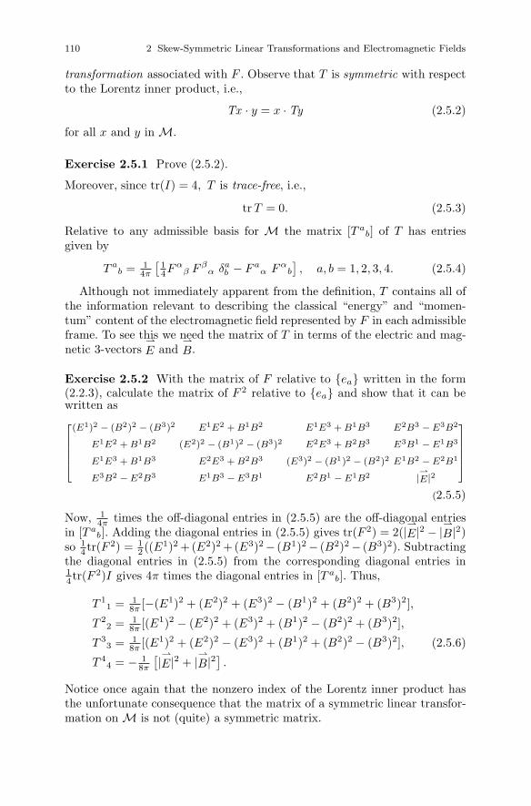
110 2 Skew-Symmetric Linear Transformations and Electromagnetic Fields
transformation associated with F . Observe that T is symmetric with respectto the Lorentz inner product, i.e.,
Tx · y = x · Ty (2.5.2)
for all x and y in M.
Exercise 2.5.1 Prove (2.5.2).
Moreover, since tr(I) = 4, T is trace-free, i.e.,
tr T = 0. (2.5.3)
Relative to any admissible basis for M the matrix [T ab] of T has entries
given by
T ab = 1
4π
[14Fα
β F βα δa
b − F aα Fα
b
], a, b = 1, 2, 3, 4. (2.5.4)
Although not immediately apparent from the definition, T contains all ofthe information relevant to describing the classical “energy” and “momen-tum” content of the electromagnetic field represented by F in each admissibleframe. To see this we need the matrix of T in terms of the electric and mag-netic 3-vectors
⇀
E and⇀
B.
Exercise 2.5.2 With the matrix of F relative to {ea} written in the form(2.2.3), calculate the matrix of F 2 relative to {ea} and show that it can bewritten as⎡⎢⎢⎢⎢⎣
(E1)2 − (B2)2 − (B3)2 E1E2 + B1B2 E1E3 + B1B3 E2B3 − E3B2
E1E2 + B1B2 (E2)2 − (B1)2 − (B3)2 E2E3 + B2B3 E3B1 − E1B3
E1E3 + B1B3 E2E3 + B2B3 (E3)2 − (B1)2 − (B2)2 E1B2 − E2B1
E3B2 − E2B3 E1B3 − E3B1 E2B1 − E1B2 |⇀E|2
⎤⎥⎥⎥⎥⎦(2.5.5)
Now, 14π
times the off-diagonal entries in (2.5.5) are the off-diagonal entriesin [T a
b]. Adding the diagonal entries in (2.5.5) gives tr(F 2) = 2(|⇀
E|2 − |⇀
B|2)so 1
4 tr(F 2) = 12 ((E1)2 +(E2)2 +(E3)2− (B1)2 − (B2)2 − (B3)2). Subtracting
the diagonal entries in (2.5.5) from the corresponding diagonal entries in14tr(F 2)I gives 4π times the diagonal entries in [T a
b]. Thus,
T 11 = 1
8π [−(E1)2 + (E2)2 + (E3)2 − (B1)2 + (B2)2 + (B3)2],
T 22 = 1
8π [(E1)2 − (E2)2 + (E3)2 + (B1)2 − (B2)2 + (B3)2],
T 33 = 1
8π[(E1)2 + (E2)2 − (E3)2 + (B1)2 + (B2)2 − (B3)2], (2.5.6)
T 44 = − 1
8π
[|⇀
E|2 + |⇀
B|2].
Notice once again that the nonzero index of the Lorentz inner product hasthe unfortunate consequence that the matrix of a symmetric linear transfor-mation on M is not (quite) a symmetric matrix.

2.5 The Energy-Momentum Transformation 111
In classical electromagnetic theory the quantity 18π
[|⇀
E|2 + |⇀
B|2](= −T 4
4
)is called the energy density measured in the given frame of reference for theelectromagnetic field with electric and magnetic 3-vectors
⇀
E and⇀
B. The3-vector 1
4π
⇀
E ×⇀
B = (E2B3 − E3B2)e1 + (E3B1 − E1B3)e2 + (E1B2 −E2B1)e3 = T 1
4e1 + T 24e2 + T 3
4e3 = −(T 4
1e1 + T 42e2 + T 4
3e3
)is called
the Poynting 3-vector and describes the energy density flux of the field. Fi-nally, the 3 × 3 matrix
[T i
j
]i,j=1,2,3
is known as the Maxwell stress tensorof the field in the given frame. Thus, the entries in the matrix of T relativeto an admissible basis all have something to say about the energy content ofthe field F measured in the corresponding frame.
Notice that the (4, 4)-entry in the matrix [T ab] of T relative to {ea} is
T 44 = −Te4 ·e4 = − 1
8π[|
⇀
E|2+|⇀
B|2]. Thus, we define, for every future-directedunit timelike vector U , the energy density of F in any admissible basis withe4 = U to be TU · U . In the sense of the following result, the energy densitycompletely determines the energy-momentum transformation.
Theorem 2.5.1 Let S and T be two nonzero linear transformations on Mwhich are symmetric with respect to the Lorentz inner product, i.e., satisfy(2.5.2). If SU · U = TU · U for every future-directed unit timelike vector U,then S = T .
Proof: Observe first that the hypothesis, together with the linearity of Sand T imply that SV · V = TV · V for all timelike vectors V . Now select abasis {Ua}4
a=1 for M, consisting exclusively of future-directed unit timelikevectors (convince yourself that such things exist). Thus, SU a ·Ua = TU a ·Ua
for each a = 1, 2, 3, 4. Next observe that, for all a, b = 1, 2, 3, 4, Lemma 1.4.3implies that Ua + Ub is timelike and future-directed so that
S(Ua + Ub) · (Ua + Ub) = T (Ua + Ub) · (Ua + Ub),SU a · Ua + 2SU a · Ub + SU b · Ub = TU a · Ua + 2TU a · Ub + TU b · Ub,
SU a · Ub = TU a · Ub.
Exercise 2.5.3 Show that
Sx · y = Tx · y (2.5.7)
for all x and y in M.
Now, let {ea}4a=1 be an orthonormal basis for M. Then (2.5.7) gives
Sea · eb = Tea · eb (2.5.8)
for all a, b = 1, 2, 3, 4. But (2.5.8) shows that the matrices of S and T relativeto {ea} are identical so S = T . �
We investigate the eigenvalues and eigenvectors of T by working in a canon-ical basis for F . First suppose F is regular and {ea} is a canonical basis forF . Then the matrix [F a
b] of F relative to {ea} has the form (2.4.9) and asimple calculation gives

112 2 Skew-Symmetric Linear Transformations and Electromagnetic Fields
[F ab]
2 =
⎡⎢⎢⎣−δ2 0 0 0
0 −δ2 0 00 0 ε2 00 0 0 ε2
⎤⎥⎥⎦so tr(F 2) = 2(ε2−δ2) and therefore [T a
b] = 14π
[ 14tr(F 2)I− [F a
b]2] is given by
[T ab] =
18π
(ε2 + δ2)
⎡⎢⎢⎣1 0 0 00 1 0 00 0 −1 00 0 0 −1
⎤⎥⎥⎦ .
det(T −λI) = 0 therefore gives (λ+ ε2+δ2
8π )2(λ− ε2+δ2
8π )2 = 0 so λ = ± ε2+δ2
8π =∓T 4
4 (the energy density). The eigenvectors corresponding to λ = ε2+δ2
8πare
obtained by solving
ε2 + δ2
8π
⎡⎢⎢⎣1 0 0 00 1 0 00 0 −1 00 0 0 −1
⎤⎥⎥⎦⎡⎢⎢⎣
v1
v2
v3
v4
⎤⎥⎥⎦ =ε2 + δ2
8π
⎡⎢⎢⎣v1
v2
v3
v4
⎤⎥⎥⎦ ,
i.e., ⎡⎢⎢⎣v1
v2
−v3
−v4
⎤⎥⎥⎦ =
⎡⎢⎢⎣v1
v2
v3
v4
⎤⎥⎥⎦ ,
so v3 = v4 = 0, whereas v1 and v2 are arbitrary. Thus, the eigenspace isSpan{e1, e2} which contains only spacelike vectors. Similarly, the eigenspacecorresponding to λ = − ε2+δ2
8πis Span{e3, e4} which contains two independent
null directions (e3 ± e4) called the principal null directions of T .If F is null and {ea} is a canonical basis, then [F a
b] has the form (2.4.14) so
[F ab]
2 =
⎡⎢⎢⎣0 0 0 00 −α2 0 α2
0 0 0 00 −α2 0 α2
⎤⎥⎥⎦and therefore tr F 2 = 0 so
[T ab] = − 1
4π[F a
b]2 =
α2
4π
⎡⎢⎢⎣0 0 0 00 1 0 −10 0 0 00 1 0 −1
⎤⎥⎥⎦ .

2.6 Motion in Constant Fields 113
Exercise 2.5.4 Show that λ = 0 is the only eigenvalue of T and that thecorresponding eigenspace is Span{e1, e3, e2 + e4}, which contains only onenull direction (that of e2 + e4), again called the principal null direction of T.
Exercise 2.5.5 Show that every eigenvector of F is also an eigenvector ofT (corresponding to a different eigenvalue, in general).
Exercise 2.5.6 Show that the energy-momentum transformation T satisfiesthe dominant energy condition, i.e., has the property that if u and v aretimelike or null and both are future-directed, then
Tu · v ≥ 0. (2.5.9)
Hint : Work in canonical coordinates for the corresponding F .
2.6 Motion in Constant Fields
Thus far we have concentrated our attention on the formal mathematicalstructure of the object we have chosen to model an electromagnetic field ata fixed point of M, that is, a skew-symmetric linear transformation. In or-der to reestablish contact with the physics of relativistic electrodynamics wemust address the issue of how a given collection of charged particles givesrise to these linear transformations at each point of M and then study howthe worldline of another charge introduced into the system will respond tothe presence of the field. The first problem we defer to Section 2.7. In thissection we consider the motion of a charged particle in the simplest of allelectromagnetic fields, i.e., those that are constant. Thus, we presume theexistence of a system of particles that determines a single skew-symmetriclinear transformation F : M → M with the property that any charged par-ticle (α, m, e) introduced into the system will experience changes in worldmomentum at every point on its worldline described by (2.1.1). More partic-ularly, we have in mind fields with the property that there exists a frame ofreference in which the field is constant and either purely magnetic (
⇀
E =⇀0 )
or purely electric (⇀
B =⇀0 ). To a reasonable degree of approximation such
fields exist in nature and are of considerable practical importance. Such afield, however, can obviously not be null (without being identically zero) sowe shall restrict our attention to the regular case and will work exclusivelyin a canonical basis.
Suppose then that F : M → M is nonzero, skew-symmetric and regular.Then there exists an admissible basis {ea}4
a=1 for M and two real numbersε ≥ 0 and δ ≥ 0 so that the matrix of F in {ea} is
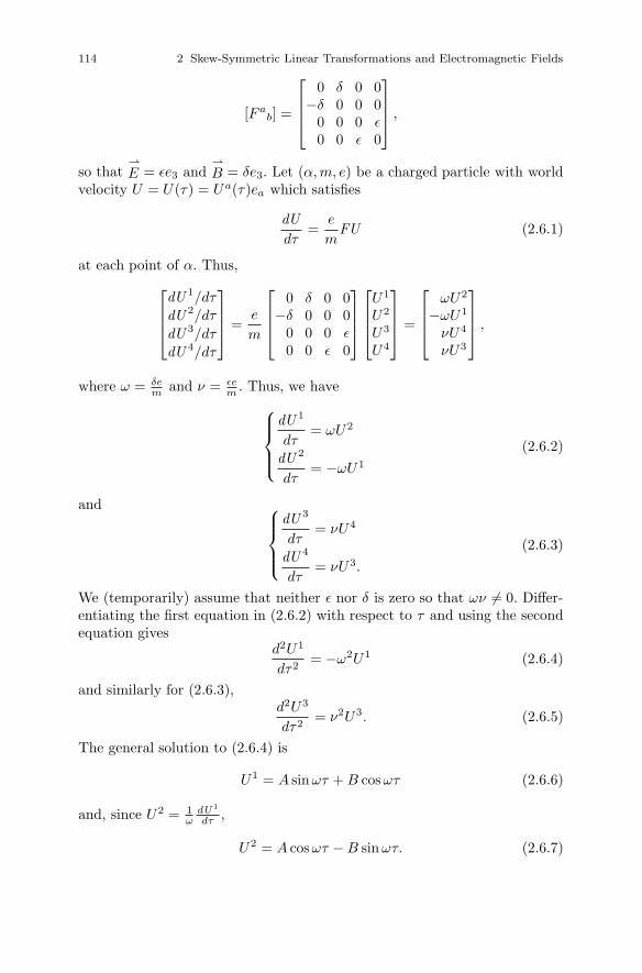
114 2 Skew-Symmetric Linear Transformations and Electromagnetic Fields
[F ab] =
⎡⎢⎢⎣0 δ 0 0
−δ 0 0 00 0 0 ε0 0 ε 0
⎤⎥⎥⎦ ,
so that⇀E = εe3 and
⇀B = δe3. Let (α, m, e) be a charged particle with world
velocity U = U(τ) = Ua(τ)ea which satisfies
dUdτ
=e
mFU (2.6.1)
at each point of α. Thus,⎡⎢⎢⎣dU 1/dτ
dU 2/dτ
dU 3/dτ
dU 4/dτ
⎤⎥⎥⎦ =e
m
⎡⎢⎢⎣0 δ 0 0
−δ 0 0 00 0 0 ε0 0 ε 0
⎤⎥⎥⎦⎡⎢⎢⎣U1
U2
U3
U4
⎤⎥⎥⎦ =
⎡⎢⎢⎣ωU2
−ωU1
νU4
νU3
⎤⎥⎥⎦ ,
where ω = δem and ν = εe
m . Thus, we have⎧⎪⎪⎨⎪⎪⎩dU 1
dτ= ωU2
dU 2
dτ= −ωU1
(2.6.2)
and ⎧⎪⎪⎨⎪⎪⎩dU 3
dτ= νU4
dU 4
dτ= νU3.
(2.6.3)
We (temporarily) assume that neither ε nor δ is zero so that ων �= 0. Differ-entiating the first equation in (2.6.2) with respect to τ and using the secondequation gives
d2U1
dτ2= −ω2U1 (2.6.4)
and similarly for (2.6.3),d2U3
dτ2= ν2U3. (2.6.5)
The general solution to (2.6.4) is
U1 = A sin ωτ + B cosωτ (2.6.6)
and, since U2 = 1ω
dU1
dτ ,
U2 = A cosωτ − B sin ωτ. (2.6.7)
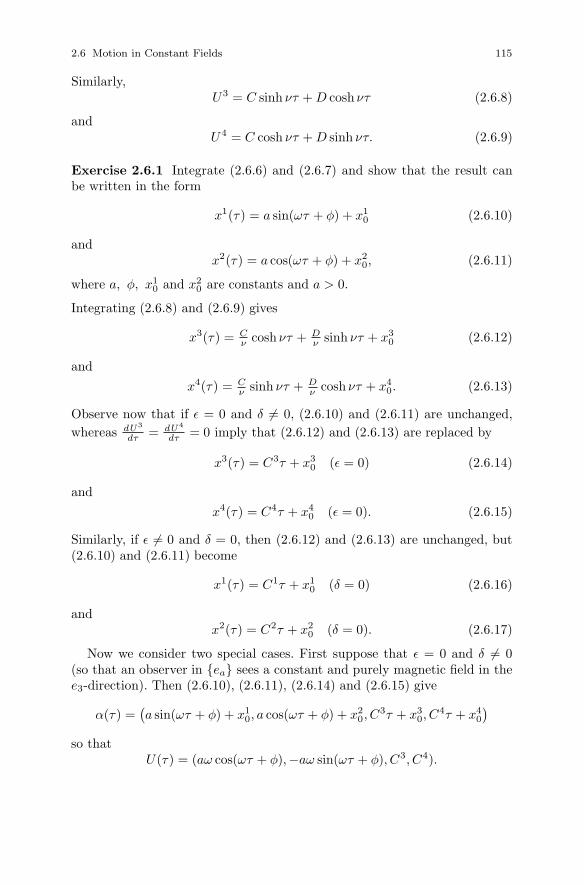
2.6 Motion in Constant Fields 115
Similarly,U3 = C sinh ντ + D cosh ντ (2.6.8)
andU4 = C cosh ντ + D sinh ντ. (2.6.9)
Exercise 2.6.1 Integrate (2.6.6) and (2.6.7) and show that the result canbe written in the form
x1(τ) = a sin(ωτ + φ) + x10 (2.6.10)
andx2(τ) = a cos(ωτ + φ) + x2
0, (2.6.11)
where a, φ, x10 and x2
0 are constants and a > 0.
Integrating (2.6.8) and (2.6.9) gives
x3(τ) = Cν cosh ντ + D
ν sinh ντ + x30 (2.6.12)
andx4(τ) = C
ν sinh ντ + Dν cosh ντ + x4
0. (2.6.13)
Observe now that if ε = 0 and δ �= 0, (2.6.10) and (2.6.11) are unchanged,whereas dU 3
dτ = dU4
dτ = 0 imply that (2.6.12) and (2.6.13) are replaced by
x3(τ) = C3τ + x30 (ε = 0) (2.6.14)
andx4(τ) = C4τ + x4
0 (ε = 0). (2.6.15)
Similarly, if ε �= 0 and δ = 0, then (2.6.12) and (2.6.13) are unchanged, but(2.6.10) and (2.6.11) become
x1(τ) = C1τ + x10 (δ = 0) (2.6.16)
andx2(τ) = C2τ + x2
0 (δ = 0). (2.6.17)
Now we consider two special cases. First suppose that ε = 0 and δ �= 0(so that an observer in {ea} sees a constant and purely magnetic field in thee3-direction). Then (2.6.10), (2.6.11), (2.6.14) and (2.6.15) give
α(τ) =(a sin(ωτ + φ) + x1
0, a cos(ωτ + φ) + x20, C
3τ + x30, C
4τ + x40
)so that
U(τ) = (aω cos(ωτ + φ),−aω sin(ωτ + φ), C3, C4).
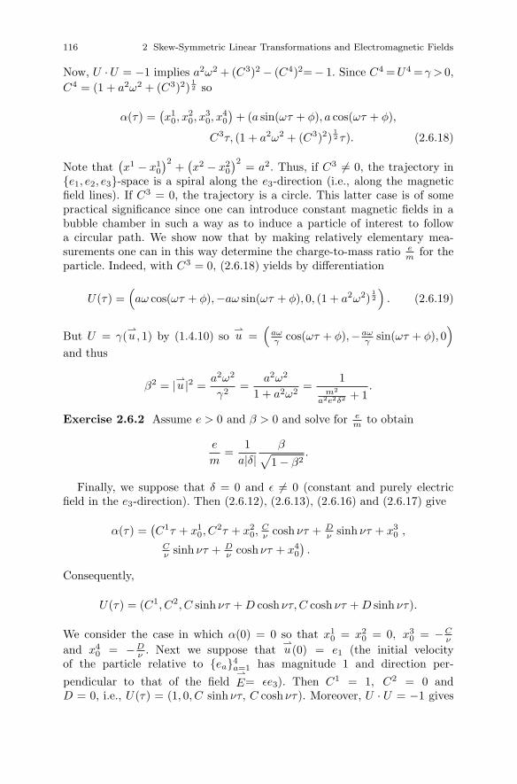
116 2 Skew-Symmetric Linear Transformations and Electromagnetic Fields
Now, U ·U = −1 implies a2ω2 + (C3)2 − (C4)2=− 1. Since C4 =U4 = γ > 0,
C4 = (1 + a2ω2 + (C3)2)12 so
α(τ) =(x1
0, x20, x
30, x
40
)+ (a sin(ωτ + φ), a cos(ωτ + φ),
C3τ, (1 + a2ω2 + (C3)2)12 τ). (2.6.18)
Note that(x1 − x1
0
)2 +(x2 − x2
0
)2 = a2. Thus, if C3 �= 0, the trajectory in{e1, e2, e3}-space is a spiral along the e3-direction (i.e., along the magneticfield lines). If C3 = 0, the trajectory is a circle. This latter case is of somepractical significance since one can introduce constant magnetic fields in abubble chamber in such a way as to induce a particle of interest to followa circular path. We show now that by making relatively elementary mea-surements one can in this way determine the charge-to-mass ratio e
mfor the
particle. Indeed, with C3 = 0, (2.6.18) yields by differentiation
U(τ) =(aω cos(ωτ + φ),−aω sin(ωτ + φ), 0, (1 + a2ω2)
12
). (2.6.19)
But U = γ(⇀u, 1) by (1.4.10) so
⇀u =
(aωγ cos(ωτ + φ),−aω
γ sin(ωτ + φ), 0)
and thus
β2 = |⇀u |2 =a2ω2
γ2=
a2ω2
1 + a2ω2=
1m2
a2e2δ2 + 1.
Exercise 2.6.2 Assume e > 0 and β > 0 and solve for em to obtain
e
m=
1a|δ|
β√1 − β2
.
Finally, we suppose that δ = 0 and ε �= 0 (constant and purely electricfield in the e3-direction). Then (2.6.12), (2.6.13), (2.6.16) and (2.6.17) give
α(τ) =(C1τ + x1
0, C2τ + x2
0,Cν cosh ντ + D
ν sinh ντ + x30 ,
Cν sinh ντ + D
ν cosh ντ + x40
).
Consequently,
U(τ) = (C1, C2, C sinh ντ + D cosh ντ, C cosh ντ + D sinh ντ).
We consider the case in which α(0) = 0 so that x10 = x2
0 = 0, x30 = −C
ν
and x40 = −D
ν . Next we suppose that⇀u(0) = e1 (the initial velocity
of the particle relative to {ea}4a=1 has magnitude 1 and direction per-
pendicular to that of the field⇀
E= εe3). Then C1 = 1, C2 = 0 andD = 0, i.e., U(τ) = (1, 0, C sinh ντ, C cosh ντ). Moreover, U · U = −1 gives
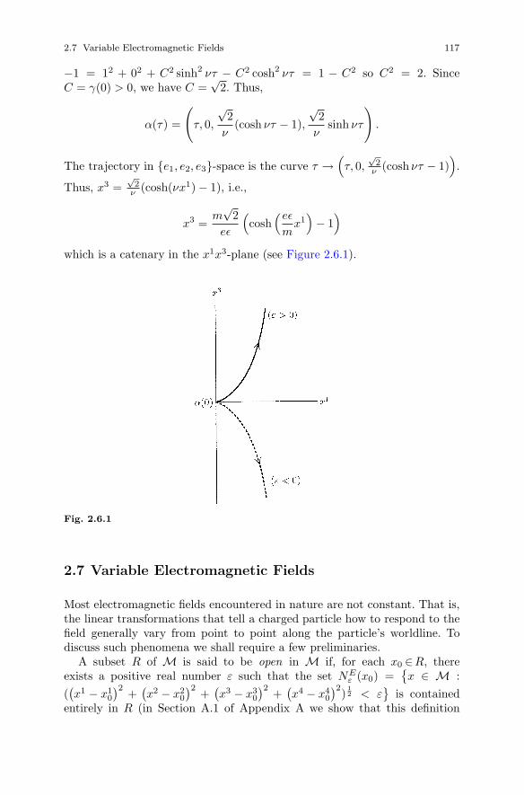
2.7 Variable Electromagnetic Fields 117
−1 = 12 + 02 + C2 sinh2 ντ − C2 cosh2 ντ = 1 − C2 so C2 = 2. SinceC = γ(0) > 0, we have C =
√2. Thus,
α(τ) =
(τ, 0,
√2
ν(cosh ντ − 1),
√2
νsinh ντ
).
The trajectory in {e1, e2, e3}-space is the curve τ →(τ, 0,
√2
ν (cosh ντ − 1)).
Thus, x3 =√
2ν (cosh(νx1) − 1), i.e.,
x3 =m√
2eε
(cosh(eε
mx1)− 1)
which is a catenary in the x1x3-plane (see Figure 2.6.1).
Fig. 2.6.1
2.7 Variable Electromagnetic Fields
Most electromagnetic fields encountered in nature are not constant. That is,the linear transformations that tell a charged particle how to respond to thefield generally vary from point to point along the particle’s worldline. Todiscuss such phenomena we shall require a few preliminaries.
A subset R of M is said to be open in M if, for each x0 ∈R, thereexists a positive real number ε such that the set NE
ε (x0) ={x ∈ M :
((x1 − x1
0
)2 +(x2 − x2
0
)2 +(x3 − x3
0
)2 +(x4 − x4
0
)2) 12 < ε
}is contained
entirely in R (in Section A.1 of Appendix A we show that this definition

118 2 Skew-Symmetric Linear Transformations and Electromagnetic Fields
does not depend on the particular admissible basis relative to which the co-ordinates are calculated). This is the usual Euclidean notion of an open setin R4 so, intuitively, one thinks of open sets in M as those sets which do notcontain any of their “boundary points”. Open sets in M will be called regionsin M. A real-valued function f : R → R defined on some region R in Mis said to be smooth if it has continuous partial derivatives of all orders andtypes with respect to x1, x2, x3 and x4 for any (and therefore all) admissi-ble coordinate systems on M. For convenience, we shall denote the partialderivative ∂f
∂xa of such a function by f,a. Now, suppose we have assigned toeach point p in some region R of M a linear transformation F (p) : M → M.Relative to an admissible basis each F (p) will have a matrix [F a
b(p)]. If theentries in this matrix are smooth on R we say that the assignment p
F−→F (p)itself is smooth. If each of the linear transformations F (p) is skew-symmetric,the smooth assignment p
F−→F (p) is a reasonable first approximation to thedefinition of an “electromagnetic field on R”. However, nature does not grantus so much freedom as to allow us to make such assignments arbitrarily. Therules by which we must play the game consist of a system of partial differ-ential equations known as “Maxwell’s equations”. In regions that are free ofcharge and in terms of the electric and magnetic 3-vectors
⇀
E and⇀
B theseequations require that
div⇀
E = 0, curl⇀
B − ∂⇀E
∂x4 =⇀0 ,
div⇀
B = 0, curl⇀
E + ∂⇀B
∂x4 =⇀0 ,
(2.7.1)
where div and curl are the familiar divergence and curl from vector analysisin R3. We now translate (2.7.1) into the language of Minkowski spacetime.
A mapping V : R → M which assigns to each p in some region R of Ma vector V (p) in M is called a vector field on R. Relative to any admissiblebasis {ea} for M we write V (p) = V a(p)ea, where V a : R → R, a = 1, 2, 3, 4,are the component functions of V relative to {ea}. A vector field is said tobe smooth if its component functions relative to any (and therefore every)admissible basis are smooth. Now consider a smooth assignment p
F−→F (p)of a linear transformation to each p ∈ R. We define a vector field div F , calledthe divergence of F , by specifying that its component functions relative toany {ea} are given by
(div F )b = ηbβFαβ,α, b = 1, 2, 3, 4. (2.7.2)
Thus, (div F )i = F αi,α for i = 1, 2, 3 and (div F )4 = −F α
4,α.

2.7 Variable Electromagnetic Fields 119
Exercise 2.7.1 A vector v in M has components relative to two admissiblebases that are related by va = Λa
bvb. Show that (2.7.2) does indeed define a
vector in M by showing that it has the correct “transformation law”:(div F
)a
= Λab(div F )b, a = 1, 2, 3, 4, (2.7.3)
where (div F )a = ηaγFαγ,α and F a
b,c = ∂∂xc F a
b. Hint : Use the change ofbasis formula
F ab = Λa
αΛbβFα
β (2.7.4)
and the chain rule to show first that
F ab,c = Λa
αΛbβΛc
γFαβ,γ . (2.7.5)
Exercise 2.7.2 Show that if pF−→F (p) and p
G−→G(p) are two smooth as-signments of linear transformations to points in the region R and F + G isdefined at each p ∈ R by (F + G)(p) = F (p) + G(p), then
div(F + G) = div F + div G. (2.7.6)
Exercise 2.7.3 Show that, if each F (p) is skew-symmetric, then, in termsof the 3-vectors
⇀
E and⇀
B,
(div F )i =[
∂⇀
E
∂x4− curl
⇀
B
]· ei, i = 1, 2, 3, (2.7.7)
(div F )4 = −div⇀
E. (2.7.8)
We conclude from Exercise 2.7.3 that the first pair of equations in (2.7.1) isequivalent to the single equation
div F = 0, (2.7.9)
where 0 is, of course, the zero vector in M.The second pair of equations in (2.7.1) is most conveniently expressed in
terms of a mathematical object closely related to F , but with a matrix thatis skew-symmetric. Thus, we define for each skew-symmetric linear transfor-mation F : M → M an associated bilinear form
F : M×M → R
byF (u, v) = u · Fv (2.7.10)
for all u and v in M. Then F is skew-symmetric, i.e., satisfies
F (v, u) = −F (u, v). (2.7.11)
120 2 Skew-Symmetric Linear Transformations and Electromagnetic Fields
The matrix [Fab ] of F relative to an admissible basis {ea} has entries given by
Fab = F (ea, eb) = ea · Feb = ηacFcb (2.7.12)
and is clearly a skew-symmetric matrix (notice how the position of the indicesis used to distinguish the matrix of F from the matrix of F ).
Exercise 2.7.4 Show that if u = uaea and v = vbeb, then F (u, v) =Fabu
avb.
The entries Fab are often called the components of F in the basis {ea}. If {ea}is another admissible basis, related to {ea} by the Lorentz transformation[Λa
b], then the components of F in the two bases are related by
Fab = ΛaαΛb
βFαβ , a, b = 1, 2, 3, 4. (2.7.13)
To prove this we observe that, by definition, Fab = ηacFcb = ηacΛc
γΛbβF γ
β .Now, (1.2.12) gives Λc
γ = ηcρηγαΛρα so Fab = ηacη
cρηγαΛραΛb
βF γβ =
ηacηcρΛρ
αΛbβ (ηγαF γ
β) = δρaΛρ
αΛbβFαβ = Λa
αΛbβFαβ as required.
Computing the quantities ηacFcb in terms of
⇀
E and⇀
B gives
[Fab ] =
⎡⎢⎢⎣0 B3 −B2 E1
−B3 0 B1 E2
B2 −B1 0 E3
−E1 −E2 −E3 0
⎤⎥⎥⎦ . (2.7.14)
Every smooth assignment pF−→F (p) of a skew-symmetric linear transfor-
mation to each point in some region in M therefore gives rise to an assignment
pF−→ F (p) which is likewise smooth in the sense that the entries in the matrix
(2.7.14) are smooth real-valued functions. As usual, we denote the derivatives∂Fab/∂xc by Fab,c.
Exercise 2.7.5 Show that the second pair of equations in (2.7.1) is equiv-alent to
Fab,c + Fbc,a + Fca,b = 0, a, b, c = 1, 2, 3, 4. (2.7.15)
Now we define an electromagnetic field on a region R in M to be a smoothassignment p
F−→F (p) of a skew-symmetric linear transformation to each
point p in R such that it and its associated assignment pF−→ F (p) of skew-
symmetric bilinear forms satisfy Maxwell’s equations (2.7.9) and (2.7.15).We remark in passing that a skew-symmetric bilinear form is often referred
to as a bivector and a smooth assignment of one such to each p in R is called a2-form on R. In the language of exterior calculus the left-hand side of (2.7.15)specifies what is called the exterior derivative of F (a 3-form) and denoteddF . Then (2.7.15) becomes
dF = 0.
2.7 Variable Electromagnetic Fields 121
Since most modern expositions of electromagnetic theory are phrased in termsof these differential forms and because it will be of interest to us in Chap-ter 3, we show next that the first pair of equations in (2.7.1) (or equivalently,(2.7.9)) can be written in a similar way. Indeed, the reader may have no-ticed a certain “duality” between the first and second pairs of equations in(2.7.1). Specifically, the first pair can be obtained from the second by for-mally changing the
⇀
B to an⇀
E and the⇀
E to −⇀
B (and adjusting a sign). Thissuggests defining the “dual” of the 2-form F to be a 2-form ∗F whose matrixat each point is obtained from (2.7.14) by formally making the substitutionsBi → Ei and Ei → −Bi so that the first pair of equations in (2.7.1) would beequivalent to d∗F = 0. In order to carry out this program rigorously we willrequire a few preliminaries. First we introduce the Levi-Civita symbol εabcddefined by
εabcd =
⎧⎪⎨⎪⎩1 if abcd is an even permutation of 1234
−1 if abcd is an odd permutation of 12340 otherwise.
Thus, for example, ε1234 = ε3412 = ε4321 = 1, ε1324 = ε3142 = −1 and ε1224 =ε1341 = 0. The Levi-Civita symbol arises most naturally in the theory ofdeterminants where it is shown that, for any 4×4 matrix M = [Ma
b]a,b=1,2,3,4,
Mαa Mβ
b Mγc M δ
d εαβγδ = εabcd(det M). (2.7.16)
Exercise 2.7.6 Let F be a skew-symmetric linear transformation on M andF its associated bilinear form. For a, b = 1, 2, 3, 4 define
∗Fab = −12εαβab Fαβ, (2.7.17)
where F αβ = ηαμ ηβν Fμν . Show that, in terms of⇀
E and⇀
B, the matrix [∗Fab ]is just (2.7.14) after the substitutions Bi → Ei and Ei → −Bi have beenmade, e.g., ∗F12 = E3. Hint : Just calculate − 1
2εαβab Fαβ in terms of
⇀
E and⇀
B for various choices of a and b and use the skew-symmetry of ∗Fab and Fab
to minimize the number of such choices you must make.
Exercise 2.7.7 Let {ea} and {ea} be two admissible bases for M, F askew-symmetric linear transformation on M and F its associated bilinearform. Define ∗Fab = − 1
2εαβab Fαβ and ∗Fab = − 12εαβab Fαβ , where Fαβ =
ηαμ ηβν Fμν and Fμν = ημσ F σν . Show that for any two vectors u = uaea =
uaea and v = vbeb = vbeb in M,
∗Fab ua vb = ∗Fab ua vb. (2.7.18)
Hint : First show that (2.7.13) is equivalent to
F ab = Λaα Λb
β Fαβ (2.7.19)
and use (2.7.16).

122 2 Skew-Symmetric Linear Transformations and Electromagnetic Fields
The equality in (2.7.18) legitimizes the following definition: If F is a skew-symmetric linear transformation on M and F is its associated bilinear formwe define the dual of F to be the bilinear form ∗F : M × M → R whosevalue at (u, v) ∈ M×M is
∗F (u, v) = ∗Fabuavb. (2.7.20)
Exercise 2.7.7 assures us that this definition is independent of the partic-ular admissible basis in which the calculations are performed. Moreover,Exercise 2.7.6 and the above-mentioned duality between the first and sec-ond pairs of equations in (2.7.1) make it clear that the first of Maxwell’sequations (2.7.9) is equivalent to
∗Fab,c + ∗Fbc,a + ∗Fca, b = 0, a, b, c = 1, 2, 3, 4, (2.7.21)
or, more concisely,d∗F = 0.
We should point out that the linear transformation F , its associated bilinearform F and the dual ∗F of F all contain precisely the same informationfrom both the mathematical and the physical points of view (examine theirmatrices in terms of
⇀
E and⇀
B). Some matters are more conveniently discussedin terms of F . For others, the appropriate choice is F or ∗F . Some calculationsare simplest when carried out with the F a
b, whereas for others one mightprefer to work with Fab , or F ab , or ∗Fab . One must become comfortable withthis sort of shifting perspective. In particular, one must develop a facilityfor the “index gymnastics” that, as we have seen already in this section, arenecessitated by such a shift. To reinforce this point, to prepare gently forChapter 3 and to derive a very important property of the energy-momentumtransformation, we pause to provide a bit more practice.
Exercise 2.7.8 Show that, for any skew-symmetric linear transformationF : M → M, 1
2FabFab = |
⇀B|2 − |
⇀E|2 and 1
4∗FabF
ab =⇀E ·
⇀B.
Next we consider a skew-symmetric linear transformation F : M → Mand its associated energy-momentum transformation T : M → M given by(2.5.1). Define a bilinear form T : M×M → R by T (u, v) = u · Tv for all(u, v) ∈ M × M. Then T is symmetric, i.e., T (v, u) = T (u, v) by (2.5.2).Now let {ea} be an admissible basis and [T a
b] the matrix of T relative to thisbasis (see (2.5.4)). For all a, b = 1, 2, 3, 4, we let Tab = T (ea, eb) = ea · Teb =ηaγ T γ
b. Then, if u = uaea and v = vbeb, we have T (u, v) = Tabuavb just as
in Exercise 2.7.4. As an exercise in index manipulation and because we willneed the result in Chapter 3 we show that Tab can be written in the form
Tab = 14π
[Faα Fb
α − 14 ηab Fαβ Fαβ
], (2.7.22)
2.7 Variable Electromagnetic Fields 123
where Fbα = ηbμ Fμα. Begin with (2.5.4).
4π Tab = 4π ηaγ T γb = ηaγ
[14 Fα
β F βα δγ
b − F γα Fα
b
]= 1
4Fαβ F β
α (ηaγ δγb ) − (ηaγ F γ
α)Fαb
= 14Fα
β F βα ηab − Faα Fα
b
= 14ηab(ηαγ Fγβ)(ηασ F βσ) − Faα ηbγ Fαγ
= 14ηab(ηαγ ηασ)Fγβ F βσ + Faα ηbγ F γα
= 14ηab δγ
σ Fγβ F βσ + Faα Fbα = 1
4 ηab Fγβ F βγ + Faα Fbα
= Faα Fbα − 1
4 ηab Fγβ F γβ = Faα Fbα − 1
4 ηab Fαβ Fαβ
as required.
Exercise 2.7.9 Show that if u = uaea and v = vbeb are timelike or null andboth are future-directed, then the dominant energy condition (2.5.9) can bewritten
Tab ua vb ≥ 0.
Now let pF−→F (p) be an electromagnetic field on some region R in M.
Assign to each p in R a linear transformation T (p) which is the energy-momentum transformation of F (p).
Exercise 2.7.10 Show that the assignment pT−→T (p) is smooth and that
div T = 0. (2.7.23)
Hints : From (2.5.4) and the product rule show that 4πT ab,c = −F a
αFαb,c −
F αbF
aα,c + 1
4
(Fα
βF βα,c + Fβ
αFαβ,c
)δab . Next show that 4πT a
b,a =−F a
α,aFαb − F a
αFαb,a + 1
2Fα
β,bFβ
α. Finally, observe that F aαFα
b,a =F aαFαb,a(F aα−Fαa)=−1
2Fαa(Fαb,a−Fab,α) and F aα,aFα
b=(ηcγF aγ,a)Fcb .
With the definitions behind us we can now spend some time looking atexamples and applications. Of course, we have already encountered severalexamples since any assignment of the same skew-symmetric linear transfor-mation to each p in R is obviously smooth and satisfies Maxwell’s equationsand these constant electromagnetic fields were investigated in Section 2.6.As our first nontrivial example we examine the so-called Coulomb field of asingle free charged particle.
We begin with a free charged particle (α, m, e). Since α : R → M we maylet W = α(R). Then W is a timelike straight line which we may assume,without loss of generality, to be a time axis with α(0) = 0. Let {ea}4
a=1 bean admissible basis with W = Span{e4}, i.e., a rest frame for the particle.We define an electromagnetic field F on M−W by specifying, at each point,its matrix relative to {ea} and decreeing that its matrix in any other basis

124 2 Skew-Symmetric Linear Transformations and Electromagnetic Fields
is obtained from the change of basis formula (2.7.4). Thus, at each point ofM − W we define the matrix of the Coulomb field F = F (x1, x2, x3, x4) of(α, m, e) relative to a rest frame for (α, m, e) to be
[F ab] = e
⎡⎢⎢⎣0 0 0 x1/r3
0 0 0 x2/r3
0 0 0 x3/r3
x1/r3 x2/r3 x3/r3 0
⎤⎥⎥⎦ , (2.7.24)
where r3 = ((x1)2 + (x2)2 + (x3)2)3/2. Thus,⇀
B =⇀0 and
⇀
E = er3
⇀r , where
⇀r = x1e1 + x2e2 + x3e3. Thus, |
⇀
E|2 = ( e2
r6 )⇀r · ⇀
r = e2
r4 so |⇀
E| = |e|r2 . Any two
bases {ea} and {ea} with W = Span{e4} are related by a rotation in R (byLemma 1.3.4). We ask the reader to show that our definition of the Coulombfield is invariant under rotations and so the field is well-defined.
Exercise 2.7.11 Suppose R = [Rab]a,b=1,2,3,4 ∈ R is a rotation and xa =
Rabx
b, a = 1, 2, 3, 4. Show that r2 = (x1)2 + (x2)2 + (x3)2 = r2 and thatthe matrix [F a
b] = R [F ab] R−1 of the Coulomb field (2.7.24) in the hatted
coordinate system is
e
⎡⎢⎢⎣0 0 0 x1/r3
0 0 0 x2/r3
0 0 0 x3/r3
x1/r3 x2/r3 x3/r3 0
⎤⎥⎥⎦ .
To justify referring to the Coulomb field as an electromagnetic field we must,of course, observe that it is smooth on the region M−W and verify Maxwell’sequations (2.7.9) and (2.7.15). Since (div F )b = ηbβFα
β,α we obtain, from(2.7.24), (div F )i = ηβiFα
β,α = Fαi,α = F 1
i,1 + F 2i,2 + F 3
i,3 + F 4i,4 =
0 + 0 + 0 + 0 = 0. Moreover,
(div F )4 = ηβ4Fαβ,α = −Fα
4,α
= −e
[∂
∂x1
(x1
r3
)+
∂
∂x2
(x2
r3
)+
∂
∂x3
(x3
r3
)+ 0
]
= − e
r6
[r3 − x1
(3r2 ∂r
∂x1
)+ r3 − x2
(3r2 ∂r
∂x2
)+ r3 − x3
(3r2 ∂r
∂x3
)]
= − e
r6
[3r3 − x1
(3r2(
x1
r
))− x2
(3r2(
x2
r
))− x3
(3r2(
x3
r
))]= − e
r6[3r3 − 3r((x1)2 + (x2)2 + (x3)2)]
= − e
r6[3r3 − 3r3] = 0.

2.7 Variable Electromagnetic Fields 125
Next observe that, from (2.7.24) and (2.7.14) we obtain
[Fab ] = e
⎡⎢⎢⎣0 0 0 x1/r3
0 0 0 x2/r3
0 0 0 x3/r3
−x1/r3 −x2/r3 −x3/r3 0
⎤⎥⎥⎦ .
Thus, (2.7.15) is automatically satisfied if all of a, b and c are in {1, 2, 3}. Theremaining possibilities are all easily checked one-by-one, e.g., if a = 1, b = 2and c = 4 we obtain
F12, 4 + F24, 1 + F41, 2 =∂
∂x4(0) +
∂
∂x1
(x2
r3
)+
∂
∂x2
(−x1
r3
)= 0 + x2
(−3r−4
(x1
r
))+ x1
(3r−4
(x2
r
))= 0.
Exercise 2.7.12 Calculate the matrix of the energy-momentum transfor-mation (2.5.1) for the Coulomb field (2.7.24) in its rest frames and show, inparticular, that T 4
4 = − e2
8πr4 .
Recalling that −T 44 is interpreted as the energy density of the electromag-
netic field F as measured in the given frame of reference, we seem forced toconclude from Exercise 2.7.12 that the total energy contained in a sphere ofradius R > 0 about a point charge (which would be obtained by integratingthe energy density over the sphere) is∫ 2π
0
∫ π
0
∫ R
0
e2
8πr4r2 sin φ dr dφ dθ =
e2
2
∫ R
0
1r2
dr
and this is an improper integral which diverges. The energy contained in sucha sphere would seem to be infinite. But then (1.8.6) would suggest an infinitemass for the charge in its rest frames. This is, of course, absurd since finiteapplied forces are found to produce nonzero accelerations of point charges.Although classical electromagnetic theory is quite beautiful and enormouslysuccessful in predicting the behavior of physical systems there are, as thiscalculation indicates, severe logical difficulties at the very foundations of thesubject and, even today, these have not been resolved to everyone’s satisfac-tion (see [Par] for more on this).
As an application we wish to calculate the field of a uniformly movingcharge. Special relativity offers a particularly elegant solution to this problemsince, according to the Relativity Principle, it matters not at all whether weview the charge as moving relative to a “fixed” frame of reference or theframe as moving relative to a “stationary” charge. Thus, in effect, we needonly transform the Coulomb field to a new reference frame, moving relative tothe rest frame of the charge. More specifically, we wish to calculate the field

126 2 Skew-Symmetric Linear Transformations and Electromagnetic Fields
due to a charge moving uniformly in a straight line with speed β relativeto some admissible frame S at the instant the charge passes through thatframe’s spatial origin. We may clearly assume, without loss of generality, thatthe motion is along the negative x1-axis and that the charge passes through(x1, x2, x3) = (0, 0, 0) at x4 = 0. If S is the frame in which the charge is at restwe need only transform the Coulomb field to S with a boost Λ(β) and evaluateat x4 = x4 = 0. The Coulomb field in S has Ei = e(xi/r3), i = 1, 2, 3, andBi = 0, i = 1, 2, 3, so, from Exercise 2.2.1,
E1 = e
(x1
r3
), E2 = eγ
(x2
r3
), E2 = eγ
(x3
r3
),
B1 = 0, B2 = eβγ
(x3
r3
), B3 = −eβγ
(x2
r3
).
We wish to express these in terms of measurements made in S. Setting x4 = 0in (1.3.29) gives x1 = γx1, x2 = x2 and x3 = x3 so that r2 = (x1)2 +(x2)2 +(x3)2 = γ2(x1)2 + (x2)2 + (x3)2, which we now denote r2. Thus,
E1 = eγ(x1/r3), E2 = eγ(x2r3), E3 = eγ(x3/r3),
B1 = 0, B2 = eβγ(x3/r3), B3 = −eβγ(x2/r3),
so⇀
E =eγ
r3
(x1e1 + x2e2 + x3e3
)=
eγ
r3
⇀
r
and⇀
B =eγ
r3
(0 · e1 + βx3e2 − βx2e3
)=
eγ
r3
(βx3e2 − βx2e3
)=
eγ
r3
∣∣∣∣∣∣e1 e2 e3
−β 0 0x1 x2 x3
∣∣∣∣∣∣=
eγ
r3
(β(−e1) ×
⇀
r)
=eγ
r3
(⇀
u ×⇀
r).
Observe that, in the nonrelativistic limit (γ ≈ 1) we obtain⇀
E ≈ e
r3
⇀
r (γ ≈ 1)
and ⇀
B ≈ e
r3
(⇀
u ×⇀
r)
(γ ≈ 1).
2.7 Variable Electromagnetic Fields 127
The first of these equations asserts that the field of a slowly moving chargeis approximately the Coulomb field, whereas the second is called the Biot-Savart Law.
Observe that the Coulomb field is certainly regular at each point of M−W
since |⇀
B|2−|⇀
E|2 = 0− |e|r2 = − |e|
r2 which is nonzero. As a nontrivial example ofan electromagnetic field that is null we consider next what are called “simple,plane electromagnetic waves”.
Let K : M → M denote some fixed, nonzero, skew-symmetric lineartransformation on M and S : M → R a smooth, nonconstant real-valuedfunction on M. Define, for each x ∈ M, a linear transformation F (x) :M → M by F (x) = S(x)K. Then the assignment x
F−→ F (x) is obviouslysmooth and one could determine necessary and sufficient conditions on Sand K to ensure that F satisfies Maxwell’s equations and so represents anelectromagnetic field. We limit our attention to a special case. For this webegin with a smooth, nonconstant function P : R → R and a fixed, nonzerovector k ∈ M. Now take S(x) = P (k · x) so that
F (x) = P (k · x)K. (2.7.25)
Observe that F takes the same value for all x ∈ M for which k · x is a con-stant, i.e., F is constant on the 3-dimensional hyperplanes {x ∈ M : k · x =r0} for some real constant r0. We now set about determining conditions onP, k and K which ensure that (2.7.25) defines an electromagnetic field on M.
Fix an admissible basis {ea}4a=1. Let k = kaea and x = xaea and suppose
the matrix of K relative to this basis is [Kab]. Then F a
b = P (k · x)Kab =
P (ηαβ kα xβ)Kab. First we consider the equation div F = 0. Now, (div F )i =
F αi,α, i = 1, 2, 3 and (div F )4 = −Fα
4,α. But
F ab,c =
∂
∂xc(P (k · x)Ka
b)
= P ′(k · x)∂
∂xc(k · x)Ka
b
soF a
b,i = P ′(k · x)kiKab, i = 1, 2, 3,
andFa
b,4 = −P ′(k · x)k4Kab.
Now, for i = 1, 2, 3,
(div F )i = F 1i,1 + F 2
i,2 + F 3i,3 + F 4
i,4
= P ′(k · x)k1K1i + P ′(k · x)k2K2
i + P ′(k · x)k3K3i − P ′(k · x)k4K4
i
= P ′(k · x)[k1K1
i + k2K2i + k3K3
i − k4K4i
].
128 2 Skew-Symmetric Linear Transformations and Electromagnetic Fields
But P ′(k · x) is not identically zero since P is not constant so (div F )i = 0implies
k1K1i + k2K2
i + k3K3i − k4K4
i = 0, i = 1, 2, 3,
that is,
ηabkaKb
i = 0, i = 1, 2, 3.
Exercise 2.7.13 Show that (div F )4 = 0 requires that ηabkaKb
4 = 0.
Thus, div F = 0 for an F given by (2.7.25) becomes
ηabkaKb
c = 0, c = 1, 2, 3, 4. (2.7.26)
Next we consider (2.7.15). For this we observe that [Fab ] = [P (k · x)Kab ] soFab,c = ∂
∂xc (P (k · x)Kab) = P ′(k · x) ∂∂xc (k · x)Kab and therefore
Fab, i = P ′(k · x)kiKab
andFab, 4 = −P (k · x)k4Kab .
Thus, Fab, c + Fbc, a + Fca, b = 0 implies
P ′(k · x)[Kab
∂
∂xc(k · x) + Kbc
∂
∂xa(k · x) + Kca
∂
∂xb(k · x)
]= 0.
Again, P ′(k · x) �≡ 0 so the expression in brackets must be zero, i.e.,
Kab∂
∂xc(k · x) + Kbc
∂
∂xa(k · x) + Kca
∂
∂xb(k · x) = 0.
If a, b and c are chosen from {1, 2, 3} this becomes
Kab kc + Kbc ka + Kca kb = 0, a, b, c = 1, 2, 3. (2.7.27)
If any of a, b or c is 4, then the terms with a k4 have a minus sign. This, and(2.7.26) also, become easier to write if we introduce the notation
kb = ηabka, b = 1, 2, 3, 4.
Thus, ki = ki for i = 1, 2, 3, but k4 = −k4. Now (2.7.26), (2.7.27) and theequation corresponding to (2.7.27) when a, b or c is 4 can be written
kbKbc = 0, c = 1, 2, 3, 4, (2.7.28)
andKab kc + Kbc ka + Kca kb = 0, a, b, c = 1, 2, 3, 4, (2.7.29)
and we have proved:

2.7 Variable Electromagnetic Fields 129
Theorem 2.7.1 Let K : M → M be a nonzero, skew-symmetric lineartransformation of M, k a nonzero vector in M and P : R → R a smooth,nonconstant function. Then F (x)= P (k · x)K defines a smooth assignmentof a skew-symmetric linear transformation to each x ∈ M and satisfiesMaxwell’s equations if and only if (2.7.28) and (2.7.29) are satisfied.
Any F (x) of the type described in Theorem 2.7.1 for which (2.7.28) and(2.7.29) are satisfied is therefore an electromagnetic field and is called a simpleplane electromagnetic wave. We have already observed that such fields areconstant on hyperplanes of the form
k1x1 + k2x2 + k3x3 − k4x4 = r0 (2.7.30)
and we now investigate some of their other characteristics. First observe thatif x and x0 are two points in the hyperplane, then the displacement vectorx − x0 between them is orthogonal to k since (x − x0) · k = x · k − x0 · k =r0− r0 = 0. Thus, k is the normal vector to these hyperplanes. We show nextthat k is necessarily null. Begin with (2.7.29). Multiply through by kc andsum as indicated.
Kabkc kc + Kbc ka kc + Kcakbkc = 0, a, b = 1, 2, 3, 4.
Thus,
Kab(k · k) + (Kbckc)ka + (Kcakc)kb = 0, a, b = 1, 2, 3, 4. (2.7.31)
But now observe that, by (2.7.28),
0 = Kbckb = ηbβKβcηαbk
α
= (ηβbηαb)Kβckα = δβ
αKβckα
= Kαckα = Kbck
b = −Kbckc.
Thus, Kbckc = 0 = Kcakc, so (2.7.31) gives Kab(k · k) = 0, for all a, b =
1, 2, 3, 4. But for some choice of a and b, Kab �= 0 so
k · k = 0
and so k is null.Next we show that a simple plane electromagnetic wave F (x) = P (k ·x)K
is null at each point x. Indeed, suppose x0 ∈ M and F (x0) = P (k · x0)Kis regular (and, in particular, nonzero). Then P (k · x0) �= 0 so K must beregular (compute
⇀
E ·⇀
B and |⇀
B|2 − |⇀
E|2). Relative to a canonical basis for Kwe have
130 2 Skew-Symmetric Linear Transformations and Electromagnetic Fields
[Kab] =
⎡⎢⎢⎣0 K1
2 0 0K2
1 0 0 00 0 0 K3
4
0 0 K43 0
⎤⎥⎥⎦ =
⎡⎢⎢⎣0 δ 0 0
−δ 0 0 00 0 0 ε0 0 ε 0
⎤⎥⎥⎦ .
We write out (2.7.28) for c = 1, 2, 3 and 4:
c = 1 : kbKb1 = 0 = k2K
21 = −δk2,
c = 2 : kbKb2 = 0 = k1K
12 = δk1,
c = 3 : kbKb3 = 0 = k4K
43 = εk4,
c = 4 : kbKb4 = 0 = k3K
34 = εk3.
Now, k is null so k4 �= 0 and therefore ε = 0. Thus, δ �= 0 so k1 = k2 = 0.Next we write out (2.7.29) with a = 1, b = 2 and c = 3:
K12k3 + K23k1 + K31k2 = 0,
K12k3 = 0,
δk3 = 0.
But δ = 0 would imply K = 0 and k3 = 0 would imply k4 = 0 and so k = 0.Either is a contradiction so F must be null at each point.
Next we tie these last two bits of information together and show that thenull vector k is actually in the principal null direction of the null transforma-tion K. We select a canonical basis for K so that
[Kab] =
⎡⎢⎢⎣0 0 0 00 0 α 00 −α 0 α0 0 α 0
⎤⎥⎥⎦ (α �= 0).
Now we write out (2.7.28) for c = 2 and 3 (c = 1 contains no informationand c = 4 is redundant):
c = 2 : kbKb2 = 0 = −α k3 =⇒ k3 = 0,
c = 3 : kbKb3 = 0 = α k2 + α k4 =⇒ k4 = −k2.
Thus, k3 = 0 and k4 = k2 so k null implies k1 = 0, i.e., k = k2(e2 + e4)in canonical coordinates. But e2 + e4 is in the principal null direction of K(Exercise 2.4.8) so we have proved half of the following theorem.
Theorem 2.7.2 Let K : M → M be a nonzero, skew-symmetric lineartransformation of M, k a nonzero vector in M and P : R → R a smoothnonconstant function. Then F (x) = P (k · x)K defines a simple plane elec-tromagnetic wave (i.e., satisfies Maxwell’s equations (2.7.28) and (2.7.29))if and only if K is null and k is in the principal null direction of K.
2.7 Variable Electromagnetic Fields 131
Proof: We have already proved the necessity. For the sufficiency we assumeK is null and k is in its principal null direction. Relative to canonical co-ordinates, the only nonzero entries in [Ka
b] and [Kab ] are K23 = K3
4 =K4
3 = −K32 = α and K23 = K34 = −K43 = −K32 = α. Moreover, k is
a multiple of e2 + e4, say, k = m(e2 + e4) so k1 = k3 = k1 = k3 = 0 andk2 = k4 = k2 = −k4 = m.
Exercise 2.7.14 Verify (2.7.28) and (2.7.29). �
Thus, we can manufacture simple plane electromagnetic waves by begin-ning with a nonzero null K : M → M, finding a nonzero null vector k in theprincipal null direction of K, selecting any smooth, non-constant P : R → R
and setting F (x) = P (k · x)K. In fact, it is even easier than this for, as wenow show, given an arbitrary nonzero null vector k we can produce a nonzeronull K : M → M which has k as a principal null direction. To see this, selecta nonzero vector l in Span{k}⊥ and set K = k ∧ l (see Exercise 2.4.7). Thus,for every v ∈ M, Kv = (k ∧ l)v = k(l · v) − l(k · v).
Exercise 2.7.15 Show that, relative to an arbitrary admissible basis{ea}, Ka
b = kalb − lakb and Kab = kalb − lakb.
Now one easily verifies (2.7.28) and (2.7.29). Indeed, kbKbc = kb(kblc − lbkc) =
(kbkb)lc − (kbl
b)kc = (k · k)lc − (k · l)kc = 0 · lc − 0 · kc = 0 since k is null andl ∈ Span{k}⊥.
Exercise 2.7.16 Verify (2.7.29).
Since K is obviously skew-symmetric we may select an arbitrary smoothnonconstant P : R → R and be assured that F (x) = P (k · x)K representsa simple plane electromagnetic wave. Most choices of P : R → R, of course,yield physically unrealizable solutions F . One particular choice that is im-portant not only because it gives rise to an observable field, but also because,mathematically, many electromagnetic waves can be regarded (via Fourieranalysis) as superpositions of such waves, is
P (t) = sinnt ,
where n is a positive integer. Thus, we begin with an arbitrary nonzero, null,skew-symmetric K : M → M and let {ea} be a canonical basis for K. Thenk = e2 + e4 is along the principal null direction of K so
F (x) = sin(nk · x)K= sin(n(e2 + e4) · x)K
= sin(n(x2 − x4))K
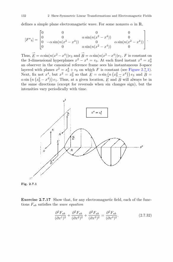
132 2 Skew-Symmetric Linear Transformations and Electromagnetic Fields
defines a simple plane electromagnetic wave. For some nonzero α in R,
[F ab] =
⎡⎢⎢⎣0 0 0 00 0 α sin(n(x2 − x4)) 00 −α sin(n(x2 − x4)) 0 α sin(n(x2 − x4))0 0 α sin(n(x2 − x4)) 0
⎤⎥⎥⎦ .
Thus,⇀
E = α sin(n(x2 −x4))e3 and⇀
B = α sin(n(x2 −x4))e1. F is constant onthe 3-dimensional hyperplanes x2 − x4 = r0. At each fixed instant x4 = x4
0
an observer in the canonical reference frame sees his instantaneous 3-spacelayered with planes x2 = x4
0 + r0 on which F is constant (see Figure 2.7.1).Next, fix not x4, but x2 = x2
0 so that⇀
E = α sin(n(x2
0 − x4))
e3 and⇀
B =α sin
(n(x2
0 − x4))
e1. Thus, at a given location,⇀
E and⇀
B will always be inthe same directions (except for reversals when sin changes sign), but theintensities vary periodically with time.
Fig. 2.7.1
Exercise 2.7.17 Show that, for any electromagnetic field, each of the func-tions Fab satisfies the wave equation
∂2Fab
(∂x1)2+
∂2Fab
(∂x2)2+
∂2Fab
(∂x3)2=
∂2Fab
(∂x4)2. (2.7.32)
2.7 Variable Electromagnetic Fields 133
Hints : Differentiate (2.7.15) with respect to xμ, multiply by ημc and sum asindicated. Then use (2.7.9) to show that two of the three terms must vanish.
Of course, not everything that satisfies a wave equation is “wavelike”(e.g., constant fields satisfy (2.7.32)). However, historically the result ofExercise 2.7.17 first suggested to Maxwell that there might exist electromag-netic fields with wavelike characteristics (and which propagate with speed 1).Our last examples are obviously of this sort and the electromagnetic theoryof light is based on the study of such solutions to Maxwell’s equations.

Chapter 3
The Theory of Spinors
3.1 Representations of the Lorentz Group
The concept of a “spinor” emerged from the work of E. Cartan on the repre-sentations of simple Lie algebras. However, it was not until Dirac employed aspecial case in the construction of his relativistically invariant equation for theelectron with “spin” that the notion acquired its present name or its currentstature in mathematical physics. In this chapter we present an elementaryintroduction to the algebraic theory of spinors in Minkowski spacetime andillustrate its utility in special relativity by recasting in spinor form muchof what we have learned about the structure of the electromagnetic field inChapter 2. We shall not stray into quantum mechanics and, in particular,will not discuss the Dirac equation (for this, see the encyclopedic monograph[PR] of Penrose and Rindler). Since it is our belief that an intuitive appreci-ation of the notion of a spinor is best acquired by approaching them by wayof group representations, we have devoted this first section to an introductionto these ideas and how they arise in special relativity. Since this section isprimarily motivational, we have not felt compelled to prove everything we sayand have, at several points, contented ourselves with a reference to a proofin the literature.
A vector v in M (e.g., a world momentum) is an object that is decribed ineach admissible frame of reference by four numbers (components) with theproperty that if v = vaea = vaea and [Λa
b] is the Lorentz transformationrelating {ea} and {ea} (i.e., eb = Λa
bea), then the components va and va arerelated by the “transformation law”
va = Λabv
b, a = 1, 2, 3, 4. (3.1.1)
A linear transformation L : M → M (e.g., an electromagnetic field) is an-other type of object that is again described in each admissible basis by a setof numbers (the entries in its matrix relative to that basis) with the property
, : An Introduction , Applied Mathematical Sciences 92,
G.L. Naber The Geometry of Minkowski Spacetime to the Mathematics of the Special Theory of RelativityDOI 10.1007/978-1-4419-7838-7_ , © Springer Science+Business Media, LLC 2012
135
3
136 3 The Theory of Spinors
that if [Lab] and [La
b] are the matrices of L in {ea} and {ea}, then
Lab = Λa
αΛbβLα
β , a, b = 1, 2, 3, 4, (3.1.2)
where[Λa
b]is the inverse of [Λa
b], i.e., ΛaαΛb
α = ΛαaΛα
b = δab ((3.1.2) is just
the familiar change of basis formula). As we found in Chapter 2, it is oftenconvenient to associate with such a linear transformation a correspondingbilinear form L : M × M → R defined by L(u, v) = u · Lv . Again, L isdescribed in each admissible basis by its set of components Lab = L(ea, eb)and components in different bases are related by a specific transformation law:
Lab = ΛaαΛb
βLαβ , a, b = 1, 2, 3, 4. (3.1.3)
Such bilinear forms can, of course, arise naturally of their own accord withoutreference to any linear transformation. The Lorentz inner product is itselfsuch an example. Indeed, if we define g : M×M → R by
g(u, v) = u · v,
then, in all admissible bases, gab = g(ea, eb) = ea · eb = ηab = g(ea, eb) = gab .In this very special case the components are the same in all admissible bases,but, nevertheless, (1.2.14) shows that the same transformation law is satisfied:
gab = ΛaαΛb
βgαβ, a, b = 1, 2, 3, 4.
The point of all of this is that examples of this sort abound in geometryand physics. In each case one has under consideration an “object” of geomet-rical or physical significance (an inner product, a world momentum vector,an electromagnetic field transformation, etc.) which is described in each ad-missible basis by a set of numerical “components” and with the property thatcomponents in different bases are related by a specific linear transformationlaw that depends on the Lorentz transformation relating the two bases. Dif-ferent “types” of objects are distinguished by their number of componentsin each basis and by the precise form of the transformation law. Classically,such objects were called “world tensors” or “4-tensors” (we give the precisedefinition shortly). World tensors are well suited to the task of expressing“Lorentz invariant” relationships since, for example, a statement which as-serts the equality, in some basis, of the components of two world tensors ofthe same type necessarily implies that their components in any other basismust also be equal (since the “transformation law” to the new basis compo-nents is the same for both). This is entirely analogous to the use of 3-vectorsin classical physics and Euclidean geometry to express relationships that aretrue in all Cartesian coordinate systems if they are true in any one. Formany years it was tacitly assumed that any valid Lorentz invariant state-ment (in particular, any law of relativistic physics) should be expressible asa world tensor equation. Dirac put an end to this in 1928 when he proposed
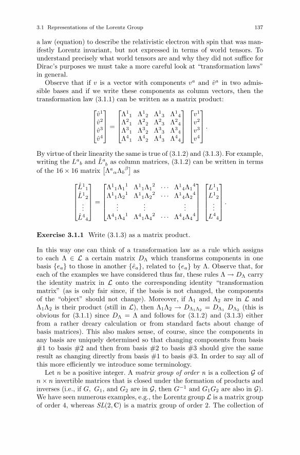
3.1 Representations of the Lorentz Group 137
a law (equation) to describe the relativistic electron with spin that was man-ifestly Lorentz invariant, but not expressed in terms of world tensors. Tounderstand precisely what world tensors are and why they did not suffice forDirac’s purposes we must take a more careful look at “transformation laws”in general.
Observe that if v is a vector with components va and va in two admis-sible bases and if we write these components as column vectors, then thetransformation law (3.1.1) can be written as a matrix product:⎡⎢⎢⎣
v1
v2
v3
v4
⎤⎥⎥⎦ =
⎡⎢⎢⎣Λ1
1 Λ12 Λ1
3 Λ14
Λ21 Λ2
2 Λ23 Λ2
4
Λ31 Λ3
2 Λ33 Λ3
4
Λ41 Λ4
2 Λ43 Λ4
4
⎤⎥⎥⎦⎡⎢⎢⎣v1
v2
v3
v4
⎤⎥⎥⎦ .
By virtue of their linearity the same is true of (3.1.2) and (3.1.3). For example,writing the La
b and Lab as column matrices, (3.1.2) can be written in terms
of the 16 × 16 matrix[Λa
αΛbβ]
as⎡⎢⎢⎢⎣L1
1
L12
...L4
4
⎤⎥⎥⎥⎦ =
⎡⎢⎢⎢⎣Λ1
1Λ11 Λ1
1Λ12 · · · Λ1
4Λ14
Λ11Λ2
1 Λ11Λ2
2 · · · Λ14Λ2
4
......
...Λ4
1Λ41 Λ4
1Λ42 · · · Λ4
4Λ44
⎤⎥⎥⎥⎦⎡⎢⎢⎢⎣
L11
L12
...L4
4
⎤⎥⎥⎥⎦ .
Exercise 3.1.1 Write (3.1.3) as a matrix product.
In this way one can think of a transformation law as a rule which assignsto each Λ ∈ L a certain matrix DΛ which transforms components in onebasis {ea} to those in another {ea}, related to {ea} by Λ. Observe that, foreach of the examples we have considered thus far, these rules Λ → DΛ carrythe identity matrix in L onto the corresponding identity “transformationmatrix” (as is only fair since, if the basis is not changed, the componentsof the “object” should not change). Moreover, if Λ1 and Λ2 are in L andΛ1Λ2 is their product (still in L), then Λ1Λ2 → DΛ1Λ2 = DΛ1 DΛ2 (this isobvious for (3.1.1) since DΛ = Λ and follows for (3.1.2) and (3.1.3) eitherfrom a rather dreary calculation or from standard facts about change ofbasis matrices). This also makes sense, of course, since the components inany basis are uniquely determined so that changing components from basis#1 to basis #2 and then from basis #2 to basis #3 should give the sameresult as changing directly from basis #1 to basis #3. In order to say all ofthis more efficiently we introduce some terminology.
Let n be a positive integer. A matrix group of order n is a collection G ofn × n invertible matrices that is closed under the formation of products andinverses (i.e., if G, G1, and G2 are in G, then G−1 and G1G2 are also in G).We have seen numerous examples, e.g., the Lorentz group L is a matrix groupof order 4, whereas SL(2,C) is a matrix group of order 2. The collection of

138 3 The Theory of Spinors
all n×n invertible matrices (with either real or complex entries) clearly alsoconstitutes a matrix group and is called the general linear group of order nand written either GL(n,R) or GL(n,C) depending on whether the entries arereal or complex. Observe that a matrix group of order n necessarily containsthe n × n identity matrix In = I since, for any G in the group, GG−1 = I.If G is a matrix group and G′ is a subset of G, then G′ is called a subgroupof G if it is closed under the formation of products and inverses, i.e., if it isitself a matrix group. For example, the set R of rotations in L is a subgroupof L (Exercise 1.3.7), SU 2 is a subgroup of SL(2,C) (Exercise 1.7.6) and,of course, any matrix group is a subgroup of some general linear group. Ahomomorphism from one matrix group G to another H is a map D : G → Hthat preserves matrix multiplication, i.e., satisfies D(G1G2) = D(G1)D(G2)whenever G1 and G2 are in G. As is customary we shall often write the imageof G under D as DG rather than D(G) and denote the action of D on G byG → DG. If G has order n and H has order m, then D necessarily carriesIn onto Im since D(In) = D(InIn) = D(In)D(In) so that D(In)(D(In))−1 =D(In)D(In)(D(In))−1 and therefore Im = D(In)Im = D(In).
Exercise 3.1.2 Show that a homomorphism D : G → H preserves inverses,i.e., that D(G−1) = (D(G))−1 for all G in G.
Exercise 3.1.3 Show that if D : G → H is a homomorphism, then its imageD(G) = {D(G) : G ∈ G} is a subgroup of H.
A homomorphism of one matrix group G into another H is also called a (finitedimensional) representation of G. For reasons that will become clear shortly,we will be particularly concerned with the representations of L and SL(2,C).If H is of order m and Vm is an m-dimensional vector space (over C if theentries in H are complex, but otherwise arbitrary), then the elements of Hcan, by selecting a basis for Vm, be regarded as linear transformations or,equivalently, as change of basis matrices on Vm. In this case the elements ofVm are called carriers of the representation. M itself may be regarded as aspace of carriers for the representation D : L → GL(4,R) of L correspond-ing to (3.1.1), i.e., the identity representation Λ → DΛ = Λ. Similarly, thevector space of linear transformations from M to M and that of bilinearforms on M act as carriers for the representations [Λa
b] →[Λa
αΛbβ]
and[Λa
b] →[Λa
αΛbβ]
corresponding to (3.1.2) and (3.1.3), respectively. It israther inconvenient, however, to have different representations of L acting oncarriers of such diverse type (vectors, linear transformations, bilinear forms)and we shall see presently that this can be avoided.
The picture we see emerging here from these few examples is really quitegeneral. Suppose that we have under consideration some geometrical or phys-ical quantity that is described in each admissible basis/frame by m uniquelydetermined numbers and suppose furthermore that these sets of numbers cor-responding to different bases are related by linear transformation laws thatdepend on the Lorentz transformation relating the bases (there are objects
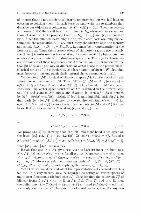
3.1 Representations of the Lorentz Group 139
of interest that do not satisfy this linearity requirement, but we shall have nooccasion to consider them). In each basis we may write the m numbers thatdescribe our object as a column matrix T = col[T1 · · ·Tm]. Then, associatedwith every Λ ∈ L there will be an m×m matrix DΛ whose entries depend onthose of Λ and with the property that T = DΛT if {ea} and {ea} are relatedby Λ. Since the numbers describing the object in each basis are uniquely de-termined, the association Λ → DΛ must carry the identity onto the identityand satisfy Λ1Λ2 → DΛ1Λ2 = DΛ1DΛ2 , i.e., must be a representation of theLorentz group. Thus, the representations of the Lorentz group are preciselythe (linear) transformation laws relating the components of physical and ge-ometrical objects of interest in Minkowski spacetime. The objects themselvesare the carriers of these representations. Of course, an m×m matrix can bethought of as acting on any m-dimensional vector space so the precise math-ematical nature of these carriers is, to a large extent, arbitrary. We shall findnext, however, that one particularly natural choice recommends itself.
We denote by M∗ the dual of the vector space M, i.e., the set of all real-valued linear functionals on M. Thus, M∗ = {f : M → R : f(αu + βv) =αf(u) + βf(v) ∀ u, v ∈ M and α, β ∈ R}. The elements of M∗ are calledcovectors. The vector space structure of M∗ is defined in the obvious way,i.e., if f and g are in M∗ and α and β are in R, then αf + βg is definedby (αf + βg)(u) = αf(u) + βg(u). If {ea} is an admissible basis for M, itsdual basis {ea} for M∗ is defined by the requirement that ea(eb) = δa
b fora, b = 1, 2, 3, 4. Let {ea} be another admissible basis for M and {ea} its dualbasis. If Λ is the element of L relating {ea} and {ea}, then
ea = Λaαeα, a = 1, 2, 3, 4, (3.1.4)
andea = Λa
αeα, a = 1, 2, 3, 4. (3.1.5)
We prove (3.1.5) by showing that the left- and right-hand sides agree onthe basis {eb} ((3.1.4) is just (1.2.15)). Of course, ea(eb) = δa
b . But also
Λaαeα(eb) = Λa
αeα(Λb
βeβ
)= Λa
αΛbβeα(eβ) = Λa
αΛbβδα
β = ΛaαΛb
α = δab
since [Λaα] and
[Λb
β]
are inverses.Recall that each v ∈ M gives rise, via the Lorentz inner product, to a
v∗ ∈ M∗ defined by v∗(u) = v · u for all u ∈ M. Moreover, if v = vaea, thenv∗ = vaea, where va = ηaαvα since va = v∗(ea) = v ·ea = (vαeα) ·ea = vα(eα ·ea) = ηaαvα. Moreover, relative to another basis, v∗ = vaea = va (Λa
αeα) =(Λa
αva) eα so vα = Λaαva and, applying the inverse, va = Λa
αvα.With this we can show that all of the representations of L considered thus
far can, in a very natural way, be regarded as acting on vector spaces ofmultilinear functionals (defined shortly). Consider first the collection T 0
2 ofbilinear forms L : M × M → R on M. If L, T ∈ T 0
2 and α ∈ R, thenthe definitions (L + T )(u, v) = L(u, v) + T (u, v) and (αL)(u, v) = αL(u, v)are easily seen to give T 0
2 the structure of a real vector space. For any two
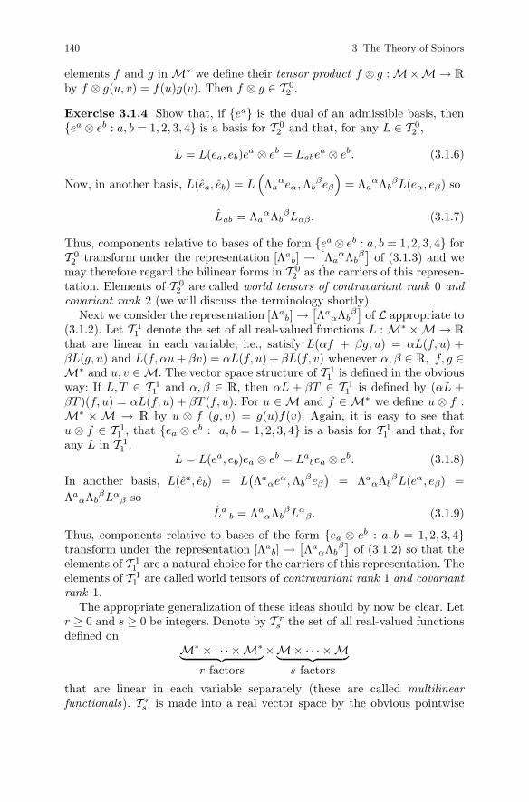
140 3 The Theory of Spinors
elements f and g in M∗ we define their tensor product f ⊗ g : M×M → R
by f ⊗ g(u, v) = f(u)g(v). Then f ⊗ g ∈ T 02 .
Exercise 3.1.4 Show that, if {ea} is the dual of an admissible basis, then{ea ⊗ eb : a, b = 1, 2, 3, 4} is a basis for T 0
2 and that, for any L ∈ T 02 ,
L = L(ea, eb)ea ⊗ eb = Labea ⊗ eb. (3.1.6)
Now, in another basis, L(ea, eb) = L(Λa
αeα, Λbβeβ
)= Λa
αΛbβL(eα, eβ) so
Lab = ΛaαΛb
βLαβ. (3.1.7)
Thus, components relative to bases of the form {ea ⊗ eb : a, b = 1, 2, 3, 4} forT 0
2 transform under the representation [Λab] →
[Λa
αΛbβ]
of (3.1.3) and wemay therefore regard the bilinear forms in T 0
2 as the carriers of this represen-tation. Elements of T 0
2 are called world tensors of contravariant rank 0 andcovariant rank 2 (we will discuss the terminology shortly).
Next we consider the representation [Λab] →
[Λa
αΛbβ]
of L appropriate to(3.1.2). Let T 1
1 denote the set of all real-valued functions L : M∗ ×M → R
that are linear in each variable, i.e., satisfy L(αf + βg, u) = αL(f, u) +βL(g, u) and L(f, αu + βv) = αL(f, u) + βL(f, v) whenever α, β ∈ R, f, g ∈M∗ and u, v ∈ M. The vector space structure of T 1
1 is defined in the obviousway: If L, T ∈ T 1
1 and α, β ∈ R, then αL + βT ∈ T 11 is defined by (αL +
βT )(f, u) = αL(f, u) + βT (f, u). For u ∈ M and f ∈ M∗ we define u ⊗ f :M∗ × M → R by u ⊗ f (g, v) = g(u)f(v). Again, it is easy to see thatu ⊗ f ∈ T 1
1 , that {ea ⊗ eb : a, b = 1, 2, 3, 4} is a basis for T 11 and that, for
any L in T 11 ,
L = L(ea, eb)ea ⊗ eb = Labea ⊗ eb. (3.1.8)
In another basis, L(ea, eb) = L(Λa
αeα, Λbβeβ
)= Λa
αΛbβL(eα, eβ) =
ΛaαΛb
βLαβ so
Lab = Λa
αΛbβLα
β. (3.1.9)
Thus, components relative to bases of the form {ea ⊗ eb : a, b = 1, 2, 3, 4}transform under the representation [Λa
b] →[Λa
αΛbβ]
of (3.1.2) so that theelements of T 1
1 are a natural choice for the carriers of this representation. Theelements of T 1
1 are called world tensors of contravariant rank 1 and covariantrank 1.
The appropriate generalization of these ideas should by now be clear. Letr ≥ 0 and s ≥ 0 be integers. Denote by T r
s the set of all real-valued functionsdefined on
M∗ × · · · ×M∗︸ ︷︷ ︸r factors
×M× · · · ×M︸ ︷︷ ︸s factors
that are linear in each variable separately (these are called multilinearfunctionals). T r
s is made into a real vector space by the obvious pointwise
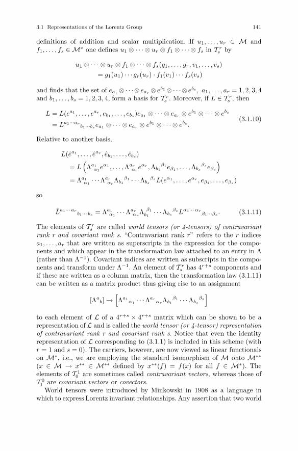
3.1 Representations of the Lorentz Group 141
definitions of addition and scalar multiplication. If u1, . . . , ur ∈ M andf1, . . . , fs ∈ M∗ one defines u1 ⊗ · · · ⊗ ur ⊗ f1 ⊗ · · · ⊗ fs in T r
s by
u1 ⊗ · · · ⊗ ur ⊗ f1 ⊗ · · · ⊗ fs(g1, . . . , gr, v1, . . . , vs)= g1(u1) · · · gr(ur) · f1(v1) · · · fs(vs)
and finds that the set of ea1 ⊗ · · ·⊗ ear ⊗ eb1 ⊗ · · ·⊗ ebs , a1, . . . , ar = 1, 2, 3, 4and b1, . . . , bs = 1, 2, 3, 4, form a basis for T r
s . Moreover, if L ∈ T rs , then
L = L(ea1 , . . . , ear , eb1 , . . . , ebs)ea1 ⊗ · · · ⊗ ear ⊗ eb1 ⊗ · · · ⊗ ebs
= La1···arb1···bsea1 ⊗ · · · ⊗ ear ⊗ eb1 ⊗ · · · ⊗ ebs .
(3.1.10)
Relative to another basis,
L(ea1 , . . . , ear , eb1 , . . . , ebs)
= L(Λa1
α1eα1 , . . . ,Λar
αreαr , Λb1
β1eβ1 , . . . ,Λbs
βseβs
)= Λa1
α1· · ·Λar
αrΛb1
β1 · · ·Λbs
βsL(eα1 , . . . , eαr , eβ1 , . . . , eβs)
so
La1···arb1··· bs = Λa1
α1· · ·Λar
αrΛ β1
b1· · ·Λbs
βsLα1···αrβ1···βs . (3.1.11)
The elements of T rs are called world tensors (or 4-tensors) of contravariant
rank r and covariant rank s. “Contravariant rank r” refers to the r indicesa1, . . . , ar that are written as superscripts in the expression for the compo-nents and which appear in the transformation law attached to an entry in Λ(rather than Λ−1). Covariant indices are written as subscripts in the compo-nents and transform under Λ−1. An element of T r
s has 4r+s components andif these are written as a column matrix, then the transformation law (3.1.11)can be written as a matrix product thus giving rise to an assignment
[Λab] →
[Λa1
α1 · · ·ΛarαrΛb1
β1 · · ·Λbs
βs
]to each element of L of a 4r+s × 4r+s matrix which can be shown to be arepresentation of L and is called the world tensor (or 4-tensor) representationof contravariant rank r and covariant rank s. Notice that even the identityrepresentation of L corresponding to (3.1.1) is included in this scheme (withr = 1 and s = 0). The carriers, however, are now viewed as linear functionalson M∗, i.e., we are employing the standard isomorphism of M onto M∗∗
(x ∈ M → x∗∗ ∈ M∗∗ defined by x∗∗(f) = f(x) for all f ∈ M∗). Theelements of T 1
0 are sometimes called contravariant vectors, whereas those ofT 0
1 are covariant vectors or covectors.World tensors were introduced by Minkowski in 1908 as a language in
which to express Lorentz invariant relationships. Any assertion that two world

142 3 The Theory of Spinors
tensors L and T are equal would be checked in a given admissible basis/frameby comparing their components La1··· ar
b1··· bs and T a1··· arb1··· bs in that basis
and, if these are indeed found to be equal in one basis, then the componentsin any other basis must necessarily also be equal since they both transformto the new basis under (3.1.11). World tensor equations are true in all admis-sible frames if and only if they are true in any one admissible frame, i.e., theyare Lorentz invariant. World tensors were introduced, in analogy with the3-vectors of classical mechanics, to serve as the basic “building blocks” fromwhich to construct the laws of relativistic (i.e., Lorentz invariant) physics. Soadmirably suited were they to this task that it was not until attempts gotunder way to reconcile the principles of relativistic and quantum mechanicsthat it was found that there were not enough “building blocks”. The reasonfor this can be traced to the fact that the underlying physically significantquantities in quantum mechanics (e.g., wave functions) are described by com-plex numbers ψ, whereas the result of a specific measurement carried out ona quantum mechanical system is a real number that depends only on quan-tities of the form ψψ and these last quantities are insensitive to changes insign, i.e., (−ψ)(−ψ) = ψψ. Consequently, ψ and −ψ give rise to precisely thesame predictions as to the result of any experiment and so must represent thesame state of the system. As a result, transforming the state’s description inone admissible frame to that in another (related to it by Λ) can be accom-plished by either one of two matrices ±DΛ. As we shall see in Section 3.5 thisambiguity in the sign is often an essential feature of the situation and cannotbe consistently removed by making one choice or the other. This fact leadsdirectly to the notion of what Penrose [PR] has called a “spinorial object”and which we shall discuss in some detail in Appendix B. For the present wewill only take these remarks as motivation for introducing what are called“two-valued representations” of the Lorentz group (intuitively, assignmentsΛ → ±DΛ of two component transformation matrices, differing only by sign,to each Λ ∈ L).
In Section 1.7 we constructed a mapping of SL(2,C) onto L called thespinor map which we now designate
Spin : SL(2,C) → L.
Spin was a homomorphism of the matrix group SL(2,C) onto the matrixgroup L that mapped the unitary subgroup SU 2 of SL(2,C) onto the rota-tion subgroup R of L and was precisely two-to-one, carrying ±G in SL(2,C)onto the same element of L (which we denote either Spin(G) = Spin(−G) orΛG = Λ−G). Next we observe that any representation D : L → H “lifts” toa representation of SL(2,C). More precisely, we define D :SL(2,C) → Hby D = D ◦ Spin. Of course, D has the property that, for every G ∈SL(2,C), D−G = D(Spin(−G)) = D(Spin(G)) = DG. Conversely, suppose

3.1 Representations of the Lorentz Group 143
D : SL(2,C) → H is a representation of SL(2,C) with the property thatD−G = DG for every G ∈ SL(2,C). We define D : L → H as follows:Let Λ ∈ L. Then there exists a G ∈ SL(2,C) such that ΛG = Λ. DefineD(Λ) = D(ΛG) = DG. Then D is a representation of L since D(Λ1Λ2) =D(ΛG1ΛG2) = D(ΛG1G2) = DG1G2 = DG1 DG2 = D(Λ1)D(Λ2). Thus, thereis a one-to-one correspondence between the representations of L and the rep-resentations of SL(2,C) that satisfy D−G = DG for all G ∈ SL(2,C).
Before proceeding with the discussion of those representations of SL(2,C)for which D−G �= DG we introduce a few more definitions. Thus, we let Gand H be arbitrary matrix groups and D : G → H a representation of G.If the order of H is m, we let Vm stand for any space of carriers for D. Asubspace S of Vm is said to be invariant under D if each DG, thought of asa linear transformation of Vm, carries S into itself, i.e., satisfies DGS ⊆ S.For example, Vm itself and the trivial subspace {0} of Vm are obviouslyinvariant under any D. If {0} and Vm are the only subspaces of Vm that areinvariant under D, then D is said to be irreducible; otherwise, D is reducible.It can be shown (see [GMS]) that all of the representations of SL(2,C) canbe constructed from those that are irreducible. Finally, two representationsD(1) : G → H1 and D(2) : G → H2, where H1 and H2 have the same order,are said to be equivalent if there exists an invertible matrix P such that
D(2)G = P−1D
(1)G P
for all G ∈ G. This is clearly equivalent to the requirement that, if Vm is aspace of carriers for both D(1) and D(2), then there exist bases {v(1)
a } and{v(2)
a } for Vm such that, for every G ∈ G, the linear transformation whosematrix relative to {v(1)
a } is D(1)G has matrix D
(2)G relative to {v(2)
a }.
Theorem 3.1.1 (Schur’s Lemma) Let G and H be matrix groups of ordern and m respectively and D : G → H an irreducible representation of G. IfA is an m × m matrix which commutes with every DG, i.e., ADG = DGAfor every G ∈ G, then A is a multiple of the identity matrix, i.e., A = λI forsome (in general, complex) number λ.
Proof: We select a space Vm of carriers and regard A and all the DG aslinear transformations on Vm. Let S = ker A. Then S is a subspace ofVm. For each s ∈ S, As = 0 implies A(DGs) = DG(As) = DG(0) = 0 soDGs ∈ S, i.e., S is invariant under D. Since D is irreducible, either S = Vm
or S = {0}. If S = Vm, then A = 0 = 0 · I and we are done. If S = {0},then A is invertible and so has a nonzero (complex) eigenvalue λ. Notice that(A − λI)DG = ADG − (λI)DG = DGA − DG(λI) = DG(A − λI) so A − λIcommutes with every DG. The argument given above shows that A − λI iseither 0 or invertible. But λ is an eigenvalue of A so A − λI is not invertibleand therefore A − λI = 0 as required. �

144 3 The Theory of Spinors
Corollary 3.1.2 Let G be a matrix group that contains −G for every G ∈ Gand D : G → H an irreducible representation of G. Then
D−G = ±DG. (3.1.12)
Proof: −G = (−I)G so D−G = D(−I)G = D−IDG and it will suffice toshow that D−I = ±I. For any G′ ∈ G, D−IDG′ = D(−I)G′ = DG′(−I) =DG′D−I so D−I commutes with each DG′ , G′ ∈ G. By Schur’s Lemma,D−I = λI for some λ. But D−ID−I = D(−I)(−I) = DI = I so (λI)(λI) =λ2 I = I. Thus, λ2 = 1 so λ = ±1 and D−I = ±I. �
Since SL(2,C) clearly contains −G for every G ∈ SL(2,C), we find thatevery irreducible representation D of SL(2,C) satisfies either D−G = DG
or D−G = −DG. As we have seen, those of the first type give representa-tions of the Lorentz group. Although those that satisfy D−G = −DG cannotlegitimately be regarded as representations of L (not being single-valued),it has become customary to refer to such a representation of SL(2,C) as atwo-valued representation of L and we shall adhere to the custom.
The problem of determining the finite-dimensional, irreducible represen-tations of SL(2,C) is thus seen to be a matter of considerable interest inmathematical physics. As it happens, these representations are well-knownand rather easy to describe. Moreover, such a description is well worth the ef-fort required to produce it since it leads inevitably to the notion of a “spinor”,which will be our major concern in this chapter.
In order to enumerate these representations of SL(2,C) it will be conve-nient to reverse our usual procedure and specify first a space of carriers and abasis and then describe the linear transformations whose matrices relative tothis basis will constitute our representations. If m ≥ 0 and n ≥ 0 are integerswe denote by Pmn the vector space of all polynomials in z and z with complexcoefficients and of degree at most m in z and at most n in z, i.e.,
Pmn = {p(z, z) = p00 + p10z + p01z + p11zz + · · ·+ pmnzmzn = prsz
rzs : prs∈C},
with the usual coefficientwise addition and scalar multiplication, i.e., p(z, z)+q(z, z) = [p00 + p10z + · · · + pmnzmzn] + [q00 + q10z + · · · + qmnzmzn] =[p00 + q00] + [p10 + q10]z + · · · + [pmn + qmn ]zmzn and αp(z, z) = (αp00) +(αp10)z+ · · · +(αpmn)zmzn. The basis implicit here is {1, z, z, zz, . . . , zmzn}so dim Pmn = (m+1)(n+1). Now, for each G =
[a bc d
]∈ SL(2,C) we define
D(m
2 , n2 )
G : Pmn → Pmn by
D( m
2 , n2 )
G (p(z, z)) = D( m
2 , n2 )
G (prszr zs) = (bz + d)m(bz + d)np(w, w),
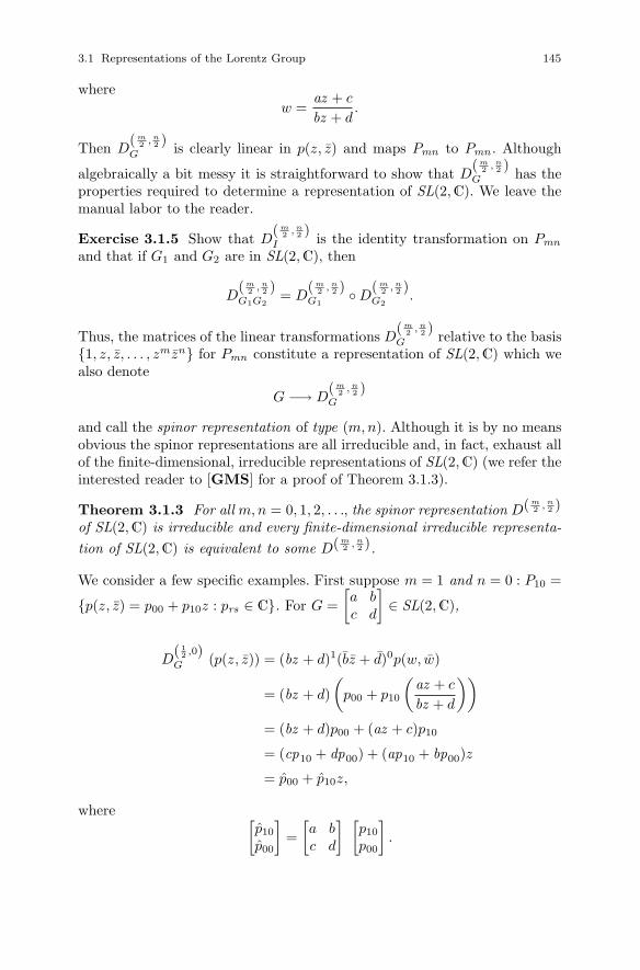
3.1 Representations of the Lorentz Group 145
wherew =
az + c
bz + d.
Then D( m
2 , n2 )
G is clearly linear in p(z, z) and maps Pmn to Pmn . Although
algebraically a bit messy it is straightforward to show that D(m
2 , n2 )
G has theproperties required to determine a representation of SL(2,C). We leave themanual labor to the reader.
Exercise 3.1.5 Show that D( m
2 , n2 )
I is the identity transformation on Pmn
and that if G1 and G2 are in SL(2,C), then
D(m
2 , n2 )
G1G2= D
( m2 , n
2 )G1
◦ D( m
2 , n2 )
G2.
Thus, the matrices of the linear transformations D(m
2 , n2 )
G relative to the basis{1, z, z, . . . , zmzn} for Pmn constitute a representation of SL(2,C) which wealso denote
G −→ D(m
2 , n2 )
G
and call the spinor representation of type (m, n). Although it is by no meansobvious the spinor representations are all irreducible and, in fact, exhaust allof the finite-dimensional, irreducible representations of SL(2,C) (we refer theinterested reader to [GMS] for a proof of Theorem 3.1.3).
Theorem 3.1.3 For all m, n = 0, 1, 2, . . ., the spinor representation D(m2 , n
2 )
of SL(2,C) is irreducible and every finite-dimensional irreducible representa-tion of SL(2,C) is equivalent to some D(m
2 , n2 ).
We consider a few specific examples. First suppose m = 1 and n = 0 : P10 =
{p(z, z) = p00 + p10z : prs ∈ C}. For G =[a bc d
]∈ SL(2,C),
D( 1
2 ,0)G (p(z, z)) = (bz + d)1(bz + d)0p(w, w)
= (bz + d)(
p00 + p10
(az + c
bz + d
))= (bz + d)p00 + (az + c)p10
= (cp10 + dp00) + (ap10 + bp00)z
= p00 + p10z,
where [p10
p00
]=[a bc d
] [p10
p00
].

146 3 The Theory of Spinors
Thus, the representation G → D( 1
2 ,0)G is given by[
a bc d
]−→ D
( 12 ,0)[a bc d
] =[a bc d
],
i.e., D( 12 ,0) is the identity representation of SL(2,C).
Exercise 3.1.6 Show in the same way that D(0, 12 ) is the conjugation rep-resentation [
a bc d
]−→ D
(0, 12 )[
a bc d
] =[a bc d
].
Exercise 3.1.7 Show that D( 12 ,0) and D(0, 1
2) are not equivalent represen-tations of SL(2,C), i.e., that there does not exist an invertible matrix P
such that P−1GP = G for all G ∈ SL(2,C). Hint : Let G =[i 00 −i
]and
P =[
0 i−i 0
]. Show that P−1GP = G and that P and its nonzero scalar mul-
tiples are the only matrices for which this is true. Now find a G′ ∈ SL(2,C)for which P−1G′P �= G′.
Before working out another example we include a few more observationsabout D( 1
2 ,0) and D(0, 12). First note that if G → DG is any representation
of SL(2,C), then the assignment G →(D−1
G
)T=(DT
G
)−1 of the trans-posed inverse of DG to each G is also a representation of SL(2,C) sinceI →
(D−1
I
)T= (I−1)T = IT = I and G1G2 → ((DG1G2)−1)T =
((DG1DG2)−1)T =(D−1
G2D−1
G1
)T=(D−1
G1
)T (D−1
G2
)T(note that inversion or
transposition alone would not accomplish this since each reverses products).Applying this, in particular, to the identity representation D( 1
2 ,0) gives
G =[a bc d
]−→ (G−1)T = (GT )−1 =
[d −c
−b a
].
Letting ε =[0 −11 0
]it is easily checked that ε−1 = −ε and
(G−1)T = ε−1Gε.
Thus, G → (G−1)T = (GT )−1 is equivalent to D( 12 ,0) and we shall denote
it D( 12 ,0). Similarly, one can define a representation D(0, 1
2 ) equivalent toconjugation by
G −→ (G−1)T = (GT )−1 = ε−1Gε.

3.1 Representations of the Lorentz Group 147
These equivalent versions of D( 12 ,0) and D(0, 12 ) as well as analogous versions
of D( m2 , n
2 ) are often convenient and we shall return to them in the nextsection.
Now let m = n = 1. Then P11 = {p(z, z) = p00 + p10z + p01z + p11zz :
prs ∈ C} and for each G =[a bc d
]∈ SL(2,C) one has
D( 1
2 , 12)
G (p(z, z)) = (bz + d)1(dz + d)1(p00 + p10w + p01w + p11ww),
where w = az+cbz+d . Multiplying out and rearranging yields
D( 1
2 , 12)G (p(z, z)) = p00 + p10z + p01z + p11zz,
where ⎡⎢⎢⎣p11
p10
p01
p00
⎤⎥⎥⎦ =
⎡⎢⎢⎣aa ab ab bbac ad bc bdac bc ad bdcc cd cd dd
⎤⎥⎥⎦⎡⎢⎢⎣p11
p10
p01
p00
⎤⎥⎥⎦ , (3.1.13)
so that
D( 1
2 , 12)[a bc d
] =
⎡⎢⎢⎣aa ab ab bbac ad bc bdac bc ad bdcc cd cd dd
⎤⎥⎥⎦ .
Proceeding in this manner with the notation currently at our disposal wouldsoon become algebraically unmanageable. For this reason we now introducenew and powerful notational devices that will constitute the language inwhich the remainder of the chapter will be written. First we rephrase theexample of D( 1
2 , 12) in these new terms. We begin by rewriting each p(z, z) as
a sum of terms of the formφAXzAzX ,
where A = 1, 0 and X = 1, 0 (the dot is used only to indicate a power of z
rather than z and 1, 0 are treated exactly as if they were 1, 0, i.e., z 0 = 1,z1 = z, 0 + 1 = 1, etc.). Thus,
p00 + p10z + p01z + p11zz = φ00z0z0 + φ10z
1z0 + φ01z0z1 + φ11z
1z1,
where φ00 = p00, φ10 = p10, φ11 = p11. With the summation convention(over A = 1, 0, X = 1, 0),
p(z, z) = φAXzAzX .
To set up another application of the summation convention we henceforthdenote the entries in G ∈ SL(2,C) as

148 3 The Theory of Spinors
G =[GA
B]
=
[G1
1 G10
G01 G0
0
]
and write the conjugate G of G as
G =[GX
Y]
=
[G1
1 G10
G01 G0
0
].
Convention: Henceforth, conjugating a term with undotted indices dots themall and introduces a bar, whereas conjugating a term with dotted indicesundots them and removes the bar. Whenever possible we will select undottedindex names from the beginning of the alphabet (A, B, C, . . .) and dottedindices from the end (. . . , X, Y , Z).
Now, if we let D( 1
2 , 12)
G (φAXzAzX) = φAXzAzX we find from (3.1.13) that⎡⎢⎢⎢⎢⎣φ11
φ10
φ01
φ00
⎤⎥⎥⎥⎥⎦ =
⎡⎢⎢⎢⎢⎣G1
1G11 G1
1G10 G1
0G11 G1
0G10
G11G0
1 G11G0
0 G10G0
1 G10G0
0
G01G1
1 G01G1
0 G00G1
1 G00G1
0
G01G0
1 G01G0
0 G00G0
1 G00G0
0
⎤⎥⎥⎥⎥⎦⎡⎢⎢⎢⎢⎣φ11
φ10
φ01
φ00
⎤⎥⎥⎥⎥⎦ (3.1.14)
which all collapses quite nicely with the summation convention to
φAX = GABGX
Y φBY , A = 1, 0, X = 1, 0. (3.1.15)
For D( 12 ,0) we would write p00 + p10z = φ0z
0 + φ1z1 = φAzA and
D( 1
2 ,0)G (φAzA) = φAzA, where
φA = GABφB , A = 1, 0. (3.1.16)
Similarly, for D(0, 12 ), p00+p01z = φ0z
0+φ1z1 = φX zX and D
(0, 12 )
G (φX zX) =φX zX , where
φX = GXY φY , X = 1, 0. (3.1.17)
Notice that the 4× 4 matrix in (3.1.14) is precisely D( 1
2 , 12)
G and that anal-ogous statements would be true of (3.1.16) and (3.1.17) if these were writtenas matrix products. The situation changes somewhat for larger m and n sowe wish to treat one more example before describing the general case. Thus,we let m = 2 and n = 1. An element p(z, z) = p00 + p10z + · · · + p21z
2z isto be written as a sum of terms of the form φA1A2XzA1zA2 zX . For example,the constant term p00 is written φ000z
0z0z0 so φ000 = p00 and p10z becomesφ100z
1z0z0 + φ010z0z1z0 and we take φ100 = φ010 = 1
2p10, and so on. Theresult is

3.1 Representations of the Lorentz Group 149
p(z, z) = φ000z0z0z0 + φ100z
1z0z0 + φ010z0z1z0
+ φ001z0z0z1 + φ101z
1z0z1 + φ011z0z1z1
+ φ110z1z1z0 + φ111z
1z1z1,
where we take
φ000 = p00, φ100 = φ010 = 12p10, φ001 = p01,
φ101 = φ011 = 12p11, φ110 = p20, φ111 = p21,
so that, in particular, φA1A2X is symmetric in A1 and A2, i.e., φA2A1X =φA1A2X for A1, A2 = 1, 0. Thus, with the summation convention,
p(z, z) = φA1A2XzA1zA2 zX = φA1A2XzA1+A2 zX .
Now,
D( 2
2 , 12 )
G (p(z, z)) =(G1
0z + G00)2 (
G10z + G0
0)1
(φA1A2XwA1+A2wX),
where
w =G1
1z + G01
G10z + G0
0,
so
D( 2
2 , 12 )
G (p(z, z)) = φA1A2X
(G1
1z + G01)A1+A2 (
G10z + G0
0)2−A1−A2
·(G1
1z + G01)X (
G10z + G0
0)1−X
= φ000
(G1
0z + G00) (
G10z + G0
0) (
G10z + G0
0)
+ φ100
(G1
1z + G01) (
G10z + G0
0) (
G10z + G0
0)
+ φ010
(G1
1z + G01) (
G10z + G0
0) (
G10z + G0
0)
+ φ110
(G1
1z + G01) (
G11z + G0
1) (
G10z + G0
0)
+ φ001
(G1
0z + G00) (
G10z + G0
0) (
G11z + G0
1)
+ φ101
(G1
1z + G01) (
G10z + G0
0) (
G11z + G0
1)
+ φ011
(G1
1z + G01) (
G10z + G0
0) (
G11z + G0
1)
+ φ111
(G1
1z + G01) (
G11z + G0
1) (
G11z + G0
1)
.

150 3 The Theory of Spinors
Multiplying out and collecting terms gives D( 2
2 , 12 )G (φA1A2XzA1+A2 zX) =
φA1A2XzA1+A2 zX , where
φA1A2X = GA1B1GA2
B2GXY φB1B2Y , A1, A2 = 1, 0, X = 1, 0. (3.1.18)
Exercise 3.1.8 Write out all terms in the expansion of D( 2
2 , 12 )G (p(z, z)) that
contain z2z and show that they can be written in the form
G1B1G1
B2G1Y φB1B2Y zB1zB2 zY
and so verify (3.1.18) for A1 = A2 = 1, X = 1. Similarly, find the constantterm and the terms with z, z2, z and zz to verify (3.1.18) for all A1, A2 and X .
Now observe that by writing the φA1A2X as a column matrix [φA1A2X ] =col[φ111 φ101 φ011 φ001 φ110 φ100 φ010 φ000], and similarly for the φB1B2Y ,(3.1.18) can be written as a matrix product⎡⎢⎢⎢⎢⎢⎣
φ111
φ101
...
φ000
⎤⎥⎥⎥⎥⎥⎦ =
⎡⎢⎢⎢⎢⎢⎣G1
1G11G1
1 G11G1
0G11 G1
0G11G1
1 · · ·G1
1G01G1
1 G11G0
0G11 G1
0G01G1
1 · · ·...
......
G01G0
1G01 G0
1G00G0
1 G00G0
1G01 · · ·
⎤⎥⎥⎥⎥⎥⎦⎡⎢⎢⎢⎢⎣φ111
φ101
...φ000
⎤⎥⎥⎥⎥⎦ .
Unlike (3.1.14), however, the 8 × 8 coefficient matrix here is not D( 2
2 , 12 )
G . In-deed, the representation G → [GA1
B1GA2B2GX
Y ] which assigns this matrixto G is not even equivalent to the spinor representation of type (2,1) sincethe latter has order (2 + 1)(1 + 1) = 6, not 8. The reason is that, in writingthe elements of P21 in the form φA1A2XzA1zA2 zX , we are not finding com-ponents relative to the basis {1, z, z, . . . , z2z} since, for example, z1z0z1 andz0z1z1 are both zz. Nevertheless, it is the transformation law (3.1.18) thatis of most interest to us.
The general case proceeds in much the same way. Pmn consists of allp(z, z) = p00 + p10z + · · · + pmnzmzn = prsz
r zs, r = 0, . . . , m, s = 0, . . . , n.Each of these is written as a sum of terms of the form
φA1···AmX1···XnzA1 · · · zAm zX1 · · · zXn ,
where A1, . . . , Am = 1, 0 and X1, . . . , Xn = 1, 0, and φA1...AmX1...Xn
is completely symmetric in A1, . . . , Am (i.e., φA1···Ai···Aj ···AmX1···Xn=
φA1···Aj ···Ai···AmX1···Xnfor all i and j) and completely symmetric in the
X1, . . . , Xn. For example,

3.1 Representations of the Lorentz Group 151
p22z2z2 = φ110···0110···0 z1z1z0 · · · z0︸ ︷︷ ︸
m
z1z1z0 · · · z0︸ ︷︷ ︸n
+ φ1010···01010···0z1z0z1z0 · · · z0z1z0z1z0 · · · z0
+ · · · + φ00···01100···011z0z0 · · · z0z1z1z0z0 · · · z0z1z1.
There are(
m2
)(n2
)terms in the sum so we may take
φA1···AmX1···Xn=
1(m2
)(n2
)p22,
where A1+ · · ·+Am = 2 and X1+ · · ·+Xn = 2. Similarly, for each 0 ≤ r ≤ mand 0 ≤ s ≤ n, if A1, . . . , Am take the values 1 and 0 with A1 + · · ·+Am = rand X1, . . . , Xn take the values 1 and 0 with X1 + · · · + Xn = s, we define
φA1···AmX1···Xn=
1(mr
)(ns
)prs .
Then
prszrzs =
∑A1 + · · · + Am = r
X1 + · · · + Xn = sAi = 1, 0
Xi = 1, 0
φA1···AmX1···XnzA1 · · · zAm zX1 · · · zXn ,
where there is no sum on the left. Summing over all r = 0, . . . , m and s =0, . . . , n and using the summation convention on both sides gives
p(z, z) = prszr zs = φA1···AmX1···Xn
zA1 · · · zAm zX1 · · · zXn
= φA1···AmX1···XnzA1+···+Am zX1+···+Xn .
Again we observe that the φ’s are symmetric in A1, . . . , Am and symmetric
in X1, . . . , Xn. Applying the transformation D(m
2 , n2 )
G to p(z, z) yields
D(m
2 , n2 )
G
(φA1···AmX1···Xn
zA1+···+Am zX1+···+Xn
)= φA1···AmX1···Xn
zA1+···+Am zX1+···+Xn ,
(3.1.19)
where
φA1···AmX1···Xn= GA1
B1 · · ·GAm
BmGX1
Y1 · · · GXn
YnφB1···BmY1···Yn,
(3.1.20)

152 3 The Theory of Spinors
and the sum is over all r = 0, . . . , m, B1+· · ·+Bm = r with B1, . . . , Bm = 1, 0and all s = 0, . . . , n, Y1 + · · · + Yn = s with Y1, . . . , Yn = 1, 0.
The transformation law (3.1.20) is typical of a certain type of “spinor”
(those of “valence”(
0 0m n
)) that we will define in the next section. For the
precise definition we wish to follow a procedure analogous to that employedin our definition of a world tensor. The idea there was that the underlyinggroup being represented (L) was the group of matrices of orthogonal trans-formations of M relative to orthonormal bases and that a world tensor couldbe identified with a multilinear functional on M and its dual. By analogywe would like to regard the elements of SL(2,C) as matrices of the structurepreserving maps of some “inner-product-like” space ß and identify “spinors”as multilinear functionals. This is, indeed, possible, although we will have tostretch our notion of “inner product” a bit.
Since the elements of SL(2,C) are 2 × 2 complex matrices, the space ß
we seek must be a 2-dimensional vector space over C. Observe that if[φ1
φ0
]and[ψ1
ψ0
]are two ordered pairs of complex numbers and G =
[GA
B]
is in
SL(2,C) and if we define[φ1
φ0
]and[ψ1
ψ0
]by
[φ1
φ0
]=
[G1
1 G10
G01 G0
0
] [φ1
φ0
]=
[G1
1φ1 + G10φ0
G01φ1 + G0
0φ0
]
and similarly for[ψ1
ψ0
], then
∣∣∣∣∣φ1 ψ1
φ0 ψ0
∣∣∣∣∣ =∣∣∣∣∣[G1
1 G10
G01 G0
0
][φ1 ψ1
φ0 ψ0
]∣∣∣∣∣=
∣∣∣∣∣G11 G1
0
G01 G0
0
∣∣∣∣∣∣∣∣∣∣φ1 ψ1
φ0 ψ0
∣∣∣∣∣=
∣∣∣∣∣φ1 ψ1
φ0 ψ0
∣∣∣∣∣and so
φ1ψ0 − φ0ψ1 = φ1ψ0 − φ0ψ1. (3.1.21)
Conversely, if (3.1.21) is satisfied, then G must be in SL(2,C). Thus, if wedefine on the vector space
C2 ={
φ =[φ1
φ0
]: φA ∈ C for A = 1, 0
}
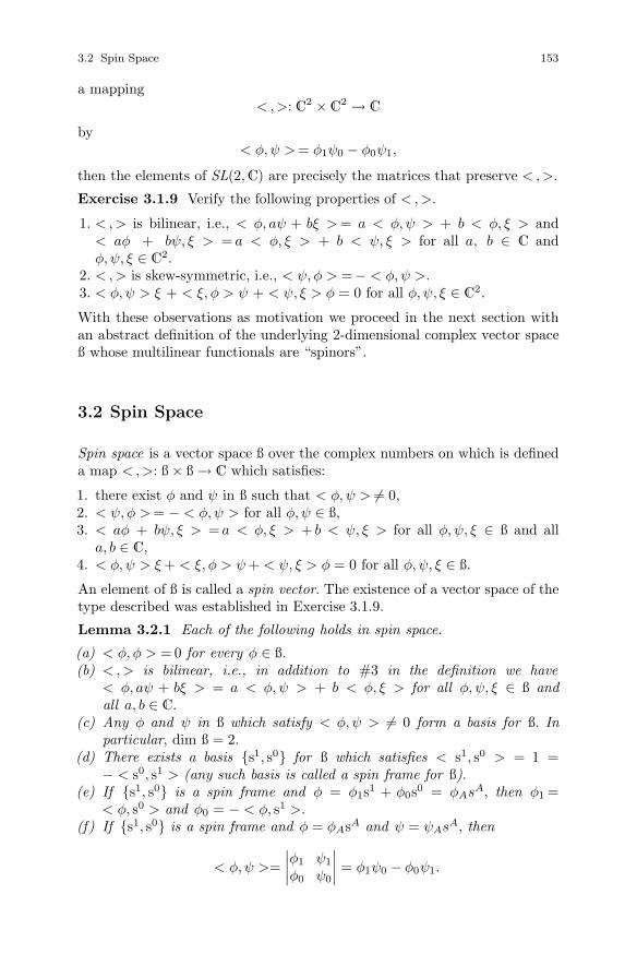
3.2 Spin Space 153
a mapping< , >: C2 × C2 → C
by< φ, ψ > = φ1ψ0 − φ0ψ1,
then the elements of SL(2,C) are precisely the matrices that preserve < , >.
Exercise 3.1.9 Verify the following properties of < , >.
1. < , > is bilinear, i.e., < φ, aψ + bξ > = a < φ, ψ > + b < φ, ξ > and< aφ + bψ, ξ > = a < φ, ξ > + b < ψ, ξ > for all a, b ∈ C andφ, ψ, ξ ∈ C2.
2. < , > is skew-symmetric, i.e., < ψ, φ > =− < φ, ψ >.3. < φ, ψ > ξ + < ξ, φ > ψ + < ψ, ξ > φ = 0 for all φ, ψ, ξ ∈ C2.
With these observations as motivation we proceed in the next section withan abstract definition of the underlying 2-dimensional complex vector spaceß whose multilinear functionals are “spinors”.
3.2 Spin Space
Spin space is a vector space ß over the complex numbers on which is defineda map < , >: ß × ß → C which satisfies:
1. there exist φ and ψ in ß such that < φ, ψ > �= 0,2. < ψ, φ > = − < φ, ψ > for all φ, ψ ∈ ß,3. < aφ + bψ, ξ > = a < φ, ξ > + b < ψ, ξ > for all φ, ψ, ξ ∈ ß and all
a, b ∈ C,4. < φ, ψ > ξ + < ξ, φ > ψ + < ψ, ξ > φ = 0 for all φ, ψ, ξ ∈ ß.
An element of ß is called a spin vector. The existence of a vector space of thetype described was established in Exercise 3.1.9.
Lemma 3.2.1 Each of the following holds in spin space.
(a) < φ, φ > = 0 for every φ ∈ ß.(b) < , > is bilinear, i.e., in addition to #3 in the definition we have
< φ, aψ + bξ > = a < φ, ψ > + b < φ, ξ > for all φ, ψ, ξ ∈ ß andall a, b ∈ C.
(c) Any φ and ψ in ß which satisfy < φ, ψ > �= 0 form a basis for ß. Inparticular, dim ß = 2.
(d) There exists a basis {s1, s0} for ß which satisfies < s1, s0 > = 1 =− < s0, s1 > (any such basis is called a spin frame for ß).
(e) If {s1, s0} is a spin frame and φ = φ1s1 + φ0s0 = φAsA, then φ1 =< φ, s0 > and φ0 = − < φ, s1 >.
(f) If {s1, s0} is a spin frame and φ = φAsA and ψ = ψAsA, then
< φ, ψ >=∣∣∣∣φ1 ψ1
φ0 ψ0
∣∣∣∣ = φ1ψ0 − φ0ψ1.
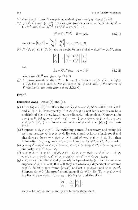
154 3 The Theory of Spinors
(g) φ and ψ in ß are linearly independent if and only if < φ, ψ > �= 0.(h) If {s1, s0} and {s1, s0} are two spin frames with s1 = G1
1s1 + G01s0 =
GA1sA and s0 = G1
0s1 + G00s0 = GA
0sA, i.e.,
sB = GAB sA, B = 1, 0, (3.2.1)
then G =[GA
B]
=[G1
1 G10
G01 G0
0
]is in SL(2,C).
(i) If {s1, s0} and {s1, s0} are two spin frames and φ = φAsA = φAsA, then[φ1
φ0
]=
[G1
1 G10
G01 G0
0
][φ1
φ0
],
i.e.,φA = GA
BφB , A = 1, 0, (3.2.2)
where the GAB are given by (3.2.1).
(j) A linear transformation T : ß → ß preserves < , > (i.e., satisfies< Tφ, Tψ > = < φ, ψ > for all φ, ψ ∈ ß) if and only if the matrix ofT relative to any spin frame is in SL(2,C).
Proof:
Exercise 3.2.1 Prove (a) and (b).
(c) From (a) and (b) it follows that < λφ, φ > = < φ, λφ > = 0 for all λ ∈ C
and all φ ∈ ß. Consequently, if < φ, ψ > �= 0, neither φ nor ψ can be amultiple of the other, i.e., they are linearly independent. Moreover, forany ξ ∈ ß, #4 gives < φ, ψ > ξ = −< ξ, φ > ψ−< ψ, ξ > φ so, since< φ, ψ > �= 0, ξ is a linear combination of φ and ψ so {φ, ψ} is a basisfor ß.
(d) Suppose < φ, ψ > �= 0. By switching names if necessary and using #2we may assume < φ, ψ > > 0. By (c), φ and ψ form a basis for ß andtherefore so do s1 = < φ, ψ >− 1
2 φ and s0 =< φ, ψ >− 12 ψ. But then
bilinearity of < , > gives < s1, s0 >= 1 and so, by #2, < s0, s1 > = −1.(e) φ = φ1s
1 + φ0s0 ⇒< φ, s0 > = φ1 < s1, s0 > + φ0 < s0, s0 > = φ1, and,
similarly, < φ, s1 > =−φ0.(f) < φ, ψ > = < φ1s
1 + φ0s0, ψ1s
1 + ψ0s0 > = φ1ψ1 < s1, s1 > + φ1ψ0
< s1, s0 > + φ0ψ1 < s0, s1 > + φ0ψ0 < s0, s0 > = φ1ψ0−φ0ψ1.(g) < φ, ψ > �= 0 implies φ and ψ linearly independent by (c). For the converse
suppose < φ, ψ > = 0. If φ = 0 they are obviously dependent so assumeφ �= 0. Select a spin frame {s1, s0} and set φ = φAsA and ψ = ψAsA.Suppose φ1 �= 0 (the proof is analogous if φ0 �= 0). By (f), < φ, ψ > = 0implies φ1ψ0 − φ0ψ1 = 0 so ψ0 = (φ0/φ1)ψ1 and therefore[
ψ1
ψ0
]=
ψ1
φ1
[φ1
φ0
],
so ψ = (ψ1/φ1)φ and φ and ψ are linearly dependent.

3.2 Spin Space 155
(h) < s1, s0 > = 1 implies 1 = < G11s1 + G0
1s0, G10s1 + G0
0s0 > =G11G1
0
< s1, s1 > + G11G0
0 < s1, s0 > + G01G1
0 < s0, s1 > + G01G0
0
< s0, s0 > = G11G0
0 − G01G1
0 = det G as required.(i) φ1s
1 + φ0s0 = φ1s
1 + φ0s0 = φ1
(G1
1s1 + G01s0)+φ0
(G1
0s1 + G00s0)
=(G1
1φ1 + G10φ0
)s1 +(G0
1φ1 + G00φ0
)s0 so the result follows by equat-
ing components.(j) Let T : ß → ß be a linear transformation and {s1, s0} a spin frame. Let[
TAB]
be the matrix of T relative to {s1, s0}. Then, for all φ and ψ in ß,Tφ = TA
BφB, Tψ = TABψB and
< φ, ψ > =∣∣∣∣φ1 ψ1
φ0 ψ0
∣∣∣∣ .Now compute
< Tφ, Tψ > =
∣∣∣∣∣T11φ1 + T1
0φ0 T11ψ1 + T1
0ψ0
T01φ1 + T0
0φ0 T01ψ1 + T0
0ψ0
∣∣∣∣∣=
∣∣∣∣∣[T1
1 T10
T01 T0
0
][φ1 ψ1
φ0 ψ0
]∣∣∣∣∣=
∣∣∣∣∣T11 T1
0
T01 T0
0
∣∣∣∣∣∣∣∣∣∣φ1 ψ1
φ0 ψ0
∣∣∣∣∣ .Thus, < Tφ, Tψ > = < φ, ψ > if and only if det
[TA
B]
= 1, i.e., if and onlyif[TA
B]∈ SL(2,C). �
Comparing (3.2.2) and (3.1.16) we see that spin vectors are a naturalchoice as carriers for the identity representation D( 1
2 ,0) of SL(2,C). To findan equally natural choice for the carrier space of the equivalent representationD( 1
2 ,0) we denote by ß∗ the dual of the vector space ß and by {s1, s0} thebasis for ß∗ dual to the spin frame {s1, s0}. Thus,
sA(sB) = δBA , A, B = 1, 0. (3.2.3)
The elements of ß∗ are called spin covectors. For each φ ∈ ß we defineφ∗ ∈ ß∗ by
φ∗(ψ)= < φ, ψ >
for every ψ ∈ ß (φ∗ is linear by (b) of Lemma 3.2.1).
Lemma 3.2.2 Every element of ß∗ is φ∗ for some φ ∈ ß.
Proof: Let f ∈ ß∗. Select a spin frame {s1, s0} and define φ ∈ ß byφ = f(s0)s1 − f(s1)s0. Then, for every ψ ∈ ß, φ∗(ψ) = < φ, ψ > = <f(s0)s1 − f(s1)s0, ψ > = f(s0) < s1, ψ > −f(s1) < s0, ψ > = −f(s0) <ψ, s1 > + f(s1) < ψ, s0 > = f(s1)ψ1+f(s0)ψ0. But f(ψ) = f(ψ1s
1+ψ0s0) =
ψ1f(s1) + ψ0f(s0) = φ∗(ψ) so f = φ∗. �
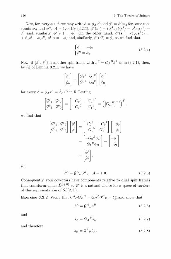
156 3 The Theory of Spinors
Now, for every φ ∈ ß, we may write φ = φAsA and φ∗ = φAsA for some con-stants φA and φA, A = 1, 0. By (3.2.3), φ∗(s1) = (φAsA)(s1) = φ1s1(s1) =φ1 and, similarly, φ∗(s0) = φ0. On the other hand, φ∗(s1)=< φ, s1 > =< φ1s
1 + φ0s0, s1 > = −φ0 and, similarly, φ∗(s0) = φ1 so we find that{
φ1 = −φ0
φ0 = φ1.(3.2.4)
Now, if {s1, s0} is another spin frame with sB = GAB sA as in (3.2.1), then,
by (i) of Lemma 3.2.1, we have[φ1
φ0
]=
[G1
1 G10
G01 G0
0
] [φ1
φ0
]
for every φ = φAsA = φAsA in ß. Letting[G1
1 G10
G01 G0
0
]=
[G0
0 −G01
−G10 G1
1
]=([
GAB]−1)T
,
we find that [G1
1 G10
G01 G0
0
][φ1
φ0
]=
[G0
0 −G01
−G10 G1
1
][−φ0
φ1
]
=
[−G0
BφB
G1BφB
]=
[−φ0
φ1
]
=
[φ1
φ0
],
so
φA = GABφB , A = 1, 0. (3.2.5)
Consequently, spin covectors have components relative to dual spin framesthat transform under D( 1
2 ,0) so ß∗ is a natural choice for a space of carriersof this representation of SL(2,C).
Exercise 3.2.2 Verify that GACGB
C = GCAGC
B = δAB and show that
sA = GABsB (3.2.6)
andsA = GA
BsB (3.2.7)
and thereforesB = GA
B sA. (3.2.8)
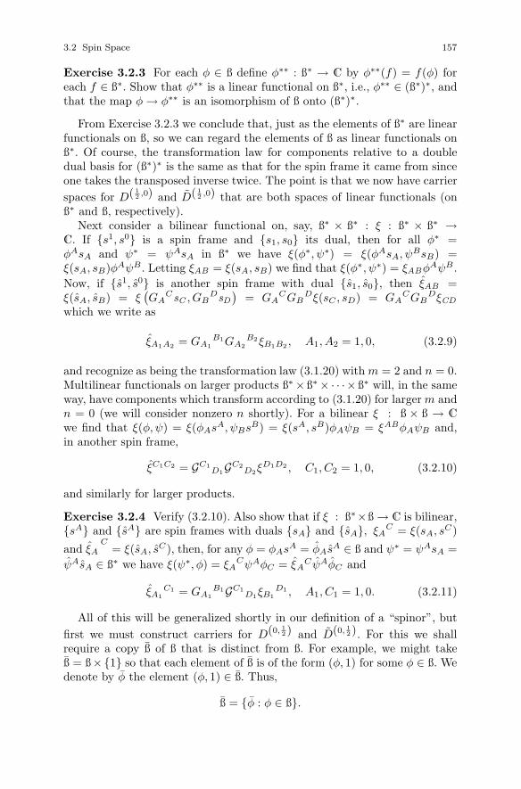
3.2 Spin Space 157
Exercise 3.2.3 For each φ ∈ ß define φ∗∗ : ß∗ → C by φ∗∗(f) = f(φ) foreach f ∈ ß∗. Show that φ∗∗ is a linear functional on ß∗, i.e., φ∗∗ ∈ (ß∗)∗, andthat the map φ → φ∗∗ is an isomorphism of ß onto (ß∗)∗.
From Exercise 3.2.3 we conclude that, just as the elements of ß∗ are linearfunctionals on ß, so we can regard the elements of ß as linear functionals onß∗. Of course, the transformation law for components relative to a doubledual basis for (ß∗)∗ is the same as that for the spin frame it came from sinceone takes the transposed inverse twice. The point is that we now have carrierspaces for D( 1
2 ,0) and D( 12 ,0) that are both spaces of linear functionals (on
ß∗ and ß, respectively).Next consider a bilinear functional on, say, ß∗ × ß∗ : ξ : ß∗ × ß∗ →
C. If {s1, s0} is a spin frame and {s1, s0} its dual, then for all φ∗ =φAsA and ψ∗ = ψAsA in ß∗ we have ξ(φ∗, ψ∗) = ξ(φAsA, ψBsB) =ξ(sA, sB)φAψB. Letting ξAB = ξ(sA, sB) we find that ξ(φ∗, ψ∗) = ξABφAψB .Now, if {s1, s0} is another spin frame with dual {s1, s0}, then ξAB =ξ(sA, sB) = ξ
(GA
CsC , GBDsD)
= GACGB
Dξ(sC , sD) = GACGB
DξCD
which we write as
ξA1A2 = GA1B1GA2
B2ξB1B2 , A1, A2 = 1, 0, (3.2.9)
and recognize as being the transformation law (3.1.20) with m = 2 and n = 0.Multilinear functionals on larger products ß∗× ß∗ × · · ·× ß∗ will, in the sameway, have components which transform according to (3.1.20) for larger m andn = 0 (we will consider nonzero n shortly). For a bilinear ξ : ß × ß → C
we find that ξ(φ, ψ) = ξ(φAsA, ψBsB) = ξ(sA, sB)φAψB = ξABφAψB and,in another spin frame,
ξC1C2 = GC1D1GC2
D2ξD1D2 , C1, C2 = 1, 0, (3.2.10)
and similarly for larger products.
Exercise 3.2.4 Verify (3.2.10). Also show that if ξ : ß∗×ß → C is bilinear,{sA} and {sA} are spin frames with duals {sA} and {sA}, ξA
C = ξ(sA, sC)
and ξAC
= ξ(sA, sC), then, for any φ = φAsA = φAsA ∈ ß and ψ∗ = ψAsA =ψAsA ∈ ß∗ we have ξ(ψ∗, φ) = ξA
CψAφC = ξACψAφC and
ξA1C1 = GA1
B1GC1D1ξB1
D1 , A1, C1 = 1, 0. (3.2.11)
All of this will be generalized shortly in our definition of a “spinor”, butfirst we must construct carriers for D(0, 1
2 ) and D(0, 12). For this we shall
require a copy ß of ß that is distinct from ß. For example, we might takeß = ß×{1} so that each element of ß is of the form (φ, 1) for some φ ∈ ß. Wedenote by φ the element (φ, 1) ∈ ß. Thus,
ß = {φ : φ ∈ ß}.

158 3 The Theory of Spinors
We define the linear space structure on ß as follows: For φ, ψ and ξ in ß andc ∈ C we have
φ + ψ = φ + ψ
andcφ = cφ
(this last being equivalent to λφ = λφ, where c and λ are the usual conjugatesof the complex numbers c and λ). Thus, the map φ → φ of ß to ß, which isobviously bijective, is a conjugate (or anti-) isomorphism, i.e., satisfies
φ + ψ −→ φ + ψ
andcφ −→ cφ.
The elements of ß are called conjugate spin vectors.Let {s1, s0} be a spin frame in ß and denote by s1 and s0 the images of s1
and s0 respectively under φ → φ. Then {s1, s0} is a basis for ß. Moreover,if φ = φ1s
1 + φ0s0 is in ß, then φ = φ1s
1 + φ0s0 (recall our notational
conventions from Section 3.1 concerning dotted indices, bars, etc.). Now, if{s1, s0} is another spin frame, related to {sA} by (3.2.6), and {¯s1, ¯s0} isits image under φ → φ, then s1 = G1
BsB = G11s
1 + G10s
0 implies ¯s1 =G 1
1s1 + G 1
0s0 and similarly for ¯s0 so
¯sX = GXY sY , X = 1, 0, (3.2.12)
and sosY = GX
Y ¯sX , Y = 1, 0. (3.2.13)
It follows that if φ = φY sY = ¯φX
¯sX , then
¯φX = GX
Y φY , X = 1, 0, (3.2.14)
andφY = GX
Y¯φX , Y = 1, 0. (3.2.15)
The elements of the dual ß∗ of ß are called conjugate spin covectors and thebases dual to {sX} and {¯sX} are denoted {sX} and {¯sX} respectively. Justas before we have
¯sX = GXY sY , X = 1, 0, (3.2.16)
andsY = GX
Y¯sX , Y = 1, 0. (3.2.17)

3.2 Spin Space 159
For each φ∗ = φAsA = φAsA ∈ ß∗ we define φ∗ ∈ ß∗ by φ∗ = φX sX =¯φX ¯sX . Then
¯φX = GX
Y φY , X = 1, 0, (3.2.18)
andφY = GX
Y ¯φX , Y = 1, 0. (3.2.19)
Before giving the general definitions we once again illustrate with a specificexample. Thus, consider a multilinear functional ξ : ß × ß × ß∗ × ß∗ → C.If φ = φAsA, ψ = ψX sX , ζ = ζBsB and ν = νY sY are in ß, ß, ß∗ and ß∗
respectively, then
ξ(φ, ψ, ζ, ν) = ξ(φAsA, ψX sX , ζBsB , νY sY )
= ξ(sA, sX , sB , sY )φAψXζB νY
= ξAXBY φAψXζB νY ,
where ξAXBY = ξ(sA, sX , sB, sY ) are the components of ξ relative to the
spin frame {s1, s0} (and the related bases for ß, ß∗ and ß∗). In another spinframe {s1, s0} we have ξ(φ, ψ, ζ, ν) = ξAX
BY φA¯ψX ζB ¯νY , where
ξAXBY = ξ(sA, ¯sX , sB, ¯sY )
= ξ(GA
A1 sA1 , GXX1
sX1 , GBB1 sB1 , GY
Y1 sY1
)= GA
A1 GXX1
GBB1 GY
Y1 ξA1X1B1Y1
which, as we shall see, is the transformation law for the components relative
to a spin frame of a “spinor of valence(
1 11 1
)”. With this we are finally
prepared to present the general definitions.
A spinor of valence(
r sm n
), also called a spinor with m undotted lower
indices, n dotted lower indices, r undotted upper indices, and s dotted upperindices is a multilinear functional
ξ : ß × · · · × ß︸ ︷︷ ︸r factors
× ß × · · · × ß︸ ︷︷ ︸s factors
× ß∗ × · · · × ß∗︸ ︷︷ ︸m factors
× ß∗ × · · · × ß∗︸ ︷︷ ︸n factors
−→ C.
If {s1, s0} is a spin frame (with associated bases {s1, s0}, {s1, s0} and {s1, s0}for ß, ß∗ and ß∗), then the components of ξ relative to {sA} are defined by
ξA1···ArX1···XsB1···BmY1···Yn
= ξ(sA1 , . . . , sAr , sX1 , . . . , sXs ,
sB1 , . . . , sBm , sY1, . . . , sYn
),
A1, . . . , Ar, B1, . . . , Bm = 1, 0,
X1, . . . , Xs, Y1, . . . , Yn = 1, 0.
(3.2.20)

160 3 The Theory of Spinors
Exercise 3.2.5 Show that, if {s1, s0} is another spin frame, then
ξA1···ArX1···XsB1···BmY1···Yn
= GA1C1 · · · GAr
Cr GX1
U1· · · GXs
UsGB1
D1 · · ·
GBm
DmG V1
Y1· · · G Vn
YnξC1···CrU1···Us
D1···DmV1···Vn.
(3.2.21)
It is traditional, particularly in the physics literature, to define a “spinorwith r contravariant and m covariant undotted indices and s contravariantand n covariant dotted indices” to be an assignment of 2r+m+s+n complexnumbers {ξA1···ArX1···Xs
B1···BmY1···Yn} to each spin frame (or, rather, an as-
signment of two such sets of numbers {± ξA1...ArX1···XsB1···BmY1···Yn
} to eachadmissible basis for M) which transform according to (3.2.21) under a changeof basis. Although our approach is more in keeping with the “coordinate-free”fashion that is currently in vogue, most calculations are, in fact, performedin terms of components and the transformation law (3.2.21). Observe alsothat, when r = s = 0, (3.2.21) coincides with the transformation law (3.2.20)for the carriers of the representation D(m
2 , n2 ) of SL(2,C). There is a dif-
ference, however, in that the φA1···AmX1···Xnconstructed in Section 3.1 are
symmetric in A1, . . . , Am and symmetric in X1, . . . , Xn and no such sym-
metry assumption is made in the definition of a spinor of valence(
0 0m n
).
The representations of SL(2,C) corresponding to the transformation laws(3.2.21) will, in general, be reducible, unlike the irreducible spinor represen-tations of Section 3.1. One final remark on the ordering of indices is apropos.The position of an index in (3.2.20) indicates the “slot” in ξ into which thecorresponding basis element is to be inserted for evaluation. For two indicesof the same type (both upper and undotted, both lower and dotted, etc.) theorder in which the indices appear is crucial since, for example, there is noreason to suppose that ξ(s1, s0, . . .) and ξ(s0, s1, . . .) are the same. However,since slots corresponding to different types of indices accept different sortsof objects (e.g., spin vectors and conjugate spin covectors) there is no reasonto insist upon any relative ordering of different types of indices and we shallnot do so. Thus, for example, ξA1A2X1
B1= ξA1X1A2
B1= ξA1
B1A2X1 etc., but
these need not be the same as ξA2A1X1B1
, etc.
3.3 Spinor Algebra
In this section we collect together the basic algebraic and computational toolsthat will be used in the remainder of the chapter. We begin by introducinga matrix that will figure prominantly in many of the calculations that arebefore us. Thus, we let ε denote the 2 × 2 matrix defined by

3.3 Spinor Algebra 161
ε =[0 −11 0
]=[ε11 ε10ε01 ε00
]= [εAB ].
Depending on the context and the requirements of the summation conventionwe will also denote the entries of ε in any of the following ways:
ε = [εAB ] = [εAB ] = [εXY ] = [εXY ].
Observe that ε−1 = −ε. Moreover, if φ and ψ are two spin vectors and {s1, s0}is a spin frame with φ = φAsA and ψ = ψBsB, then, with the summationconvention, εABψAφB = ε10ψ1φ0 + ε01ψ0φ1 = φ1ψ0 −φ0ψ1 = < φ, ψ >. Alsolet φ∗ = φAsA and ψ∗ = ψAsA be the corresponding spin covectors.
Exercise 3.3.1 Verify each of the following:
< φ, ψ > = εABψAφB = −εABφAψB , (3.3.1)
φA = εABφB = −φBεBA, (3.3.2)
φA = φBεBA = −εABφB , (3.3.3)
φAψA = < φ, ψ > = −φAψA, (3.3.4)
εAC εBC = δAB = εCAεCB , (3.3.5)
(εCBφB)εCA = φA and εAC (φBεBC ) = φA, (3.3.6)
εABεAB = 2 = εAB εAB . (3.3.7)
Of course, each of the identities (3.3.1)–(3.3.7) has an obvious “barred anddotted” version, e.g., (3.3.6) would read (εZY φY )εZX = φX . In addition tothese we record several more identities that will be used repeatedly in thesequel.
εAB εCD + εAC εDB + εADεBC = 0, A, B, C, D = 1, 0. (3.3.8)
To prove (3.3.8) we suppose first that A = 1. Thus, we consider ε1BεCD +ε1CεDB + ε1DεBC . If B = 1 this becomes ε1CεD1 + ε1Dε1C . C = 1 or D = 1gives 0 for both terms. For C = 0 and D = 0 we obtain ε10ε01 + ε10ε10 =(−1)(1) + (−1)(−1) = 0. On the other hand, if B = 0 we have ε10εCD +ε1CεD0 + ε1Dε0C . C = D gives 0 for each term. For C = 0 and D = 1 weobtain ε10ε01 + ε10ε10 + ε11ε00 = (−1)(1) + (−1)(−1) + 0 = 0. If C = 1 andD = 0, ε10ε10 + ε11ε00 + ε10ε01 = (−1)(−1) + 0 + (−1)(1) = 0. Thus, (3.3.8)is proved if A = 1 and the argument is the same if A = 0. Next we show thatif G =
[GA
B]∈ SL(2,C), then
GAA1GB
B1εA1B1 = εAB , A, B = 1, 0. (3.3.9)

162 3 The Theory of Spinors
This follows from
GAA1GB
B1εA1B1 = GA1GB
0ε10 + GA0GB
1ε01
= GA0GB
1 − GA1GB
0
=
⎧⎪⎨⎪⎩0 , if A = B
det G, if A = 0, B = 1− det G, if A = 1, B = 0
= εAB (det G)= εAB
since det G = 1. Similarly, if G = [GAB ] = ([GA
B]−1)T ,
GAA1GB
B1εA1B1 = εAB , A, B = 1, 0, (3.3.10)
and both (3.3.9) and (3.3.10) have barred and dotted versions. Observethat the bilinear form < , > : ß × ß → C is, according to our definitions in
Section 3.2, a spinor of valence(
2 00 0
)and has components in any spin
frame given by < sA, sB > = −εAB and that (3.2.10), with εAB = εAB , sim-ply confirms the appropriate transformation law. In the same way, (3.3.9)asserts that the εAB can be regarded as the (constant) components of a
spinor of valence(
0 02 0
), whereas the barred and dotted versions of these
make similar assertions about the εXY and εXY .
Exercise 3.3.2 Write out explicitly the bilinear forms (spinors) whose com-ponents relative to every spin frame are εAB , εXY and εXY .
The first equality in (3.3.2) asserts that, given a spin vector φ and thecorresponding spin covector φ∗, then, relative to any spin frame, the com-ponents of φ∗ = φAsA are mechanically retrievable from those of φ = φBsB
by forming the sum εABφB . This process is called raising the index of φB .Similarly, obtaining the φA from the φB according to (3.3.3) by computingφBεBA is termed lowering the index of φB . Due to the skew-symmetry ofthe εAB care must be exercised in arranging the order of the factors and theplacement of the indices when carrying out these processes. As an aid to thememory, one “raises on the left and lowers on the right” with the summed in-dices “adjacent and descending to the right”. The equalities in (3.3.6) assertthat these two operations are consistent, i.e., that lowering a raised index orvice versa returns the original component. The operations of raising and low-ering indices extend easily to higher valence spinors. Consider, for example, a

3.3 Spinor Algebra 163
spinor ξ of valence(
2 01 0
). In each spin frame ξ has components ξAB
C and
we now define numbers ξAB
C in this frame by
ξAB
C = ξA1BCεA1A.
In another spin frame we have ξAB
C = ξA1BCεA1A and we now show that
ξAB
C = GAA1GB
B1GCC1ξA1
B1C1
, (3.3.11)
so that the ξAB
C transform as the components of a spinor of valence(
1 02 0
).
This last spinor we shall say is obtained from ξ by “lowering the first (undot-ted) upper index”. To prove (3.3.11) we use (3.3.9) and the transformationlaw for the ξAB
C as follows:
ξAB
C = ξA1BCεA1A =
(GA1
A2GBB1GC
C1ξA2B1C1
) (GA1
A3GAA4εA3A4
)=(GA1
A2GA1A3) (
GBB1GC
C1GAA4) (
ξA2B1C1
εA3A4
)= δA3
A2
(GB
B1GCC1GA
A4) (
ξA2B1C1
εA3A4
)=(GB
B1GCC1GA
A4) (
ξA3B1C1
εA3A4
)= GB
B1GCC1GA
A4ξA4B1
C1
= GAA4GB
B1GCC1ξA4
B1C1
= GAA1GB
B1GCC1ξA1
B1C1
as required.
Exercise 3.3.3 With ξ as above, let ξABC = εCC1ξABC1
in each spin frame.Show that ξABC = GA
A1GBB1GC
C1ξA1B1C1 and conclude that the ξABC
determine a spinor of valence(
3 00 0
).
The calculations in these last examples make it clear that a spinor of anyvalence can have any one of its lower (upper) indices raised (lowered) to yielda spinor with one more upper (lower) index. Applying this to the constantspinors εAB and εAB and using (3.3.5) yields the following useful identities.
εAB = εBC εAC = δB
A (3.3.12)
and
εAB = εAC εCB = −δA
B. (3.3.13)
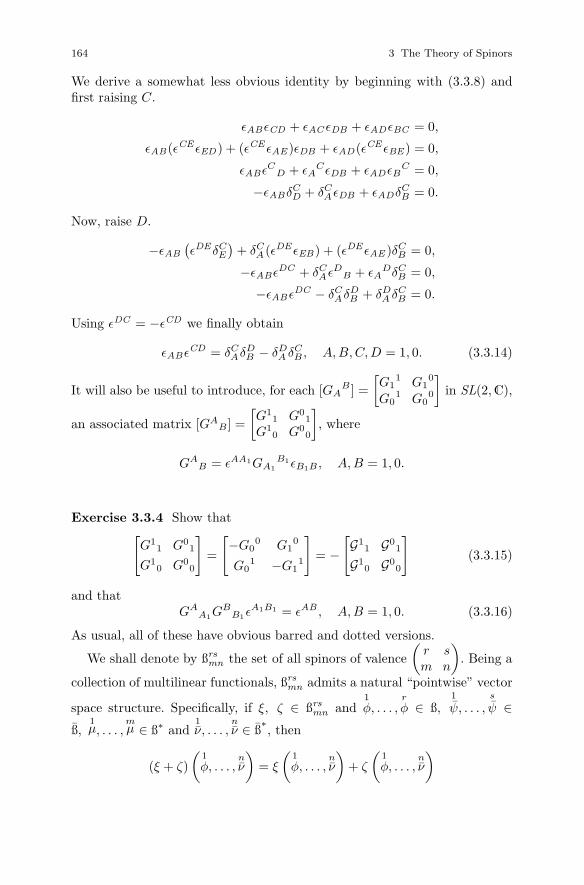
164 3 The Theory of Spinors
We derive a somewhat less obvious identity by beginning with (3.3.8) andfirst raising C.
εABεCD + εAC εDB + εADεBC = 0,
εAB(εCEεED ) + (εCE εAE )εDB + εAD(εCEεBE ) = 0,
εABεCD + εA
CεDB + εADεBC = 0,
−εABδCD + δC
AεDB + εADδCB = 0.
Now, raise D.
−εAB
(εDEδC
E
)+ δC
A (εDE εEB) + (εDE εAE )δCB = 0,
−εABεDC + δCAεD
B + εADδC
B = 0,
−εAB εDC − δCAδD
B + δDA δC
B = 0.
Using εDC = −εCD we finally obtain
εABεCD = δCAδD
B − δDA δC
B , A, B, C, D = 1, 0. (3.3.14)
It will also be useful to introduce, for each [GAB ] =
[G1
1 G10
G01 G0
0
]in SL(2,C),
an associated matrix [GAB] =
[G1
1 G01
G10 G0
0
], where
GAB = εAA1GA1
B1εB1B , A, B = 1, 0.
Exercise 3.3.4 Show that[G1
1 G01
G10 G0
0
]=
[−G0
0 G10
G01 −G1
1
]= −[G1
1 G01
G10 G0
0
](3.3.15)
and thatGA
A1GB
B1εA1B1 = εAB , A, B = 1, 0. (3.3.16)
As usual, all of these have obvious barred and dotted versions.
We shall denote by ßrsmn the set of all spinors of valence
(r sm n
). Being a
collection of multilinear functionals, ßrsmn admits a natural “pointwise” vector
space structure. Specifically, if ξ, ζ ∈ ßrsmn and
1
φ, . . . ,r
φ ∈ ß,1
ψ, . . . ,s
ψ ∈ß,
1μ, . . . ,
mμ ∈ ß∗ and
1ν, . . . ,
nν ∈ ß∗, then
(ξ + ζ)(
1
φ, . . . ,nν
)= ξ
(1
φ, . . . ,nν
)+ ζ
(1
φ, . . . ,nν
)

3.3 Spinor Algebra 165
and, for α ∈ C,
(αξ)(
1
φ, . . . ,nν
)= α
(ξ
(1
φ, . . . ,nν
)).
If {s1, s0} is a spin frame, {s1, s0} its dual basis for ß∗, {s1, s0} the corre-sponding conjugate basis for ß and {s1, s0} its dual, we define sA1⊗. . .⊗sAr⊗sX1
⊗· · ·⊗sXs⊗sB1⊗· · ·⊗sBm⊗sY1⊗· · ·⊗sYn , abbreviated sA1⊗· · ·⊗sYn , by
sA1 ⊗ · · · ⊗ sYn
(1
φ, . . . ,nν
)= sA1
(1
φ
)· · · sYn
(nν)
=1
φ A1 · · ·nν Yn
.
Thus, for example, in ß1110 we have s1 ⊗ s0 ⊗ s0 defined by s1 ⊗ s0 ⊗ s0 (φ, ψ, μ)
= s1(φ)s0(ψ)s0(μ) = φ1ψ0μ0, where φ = φAsA, ψ = ψX sX and μ = μAsA.
For ξ ∈ ßrsmn we define
ξA1···XsB1···Yn
= ξ(sA1 , . . . , sXs , sB1 , . . . , sYn
)(3.3.17)
for Ai, Bi = 1, 0 and Xi, Yi = 1, 0.
Exercise 3.3.5 Show that the elements sA1 ⊗ · · · ⊗ sYn of ßrsmn are linearly
independent and that any ξ ∈ ßrsmn can be written
ξ = ξA1···XsB1···Yn
sA1 ⊗ · · · ⊗ sXs⊗ sB1 ⊗ · · · ⊗ sYn .
From Exercise 3.3.5 we conclude that the sA1 ⊗ · · · ⊗ sYn form a basis forßrsmn which therefore has dimension 2r+s+m+n. For each ξ ∈ ßrs
mn the numbersξA1···Xs
B1···Yndefined by (3.3.17) are the components of ξ relative to the basis
{sA1 ⊗ · · · ⊗ sYn} and, in terms of them, the linear operations on ßrsmn can be
expressed as
(ξ + ζ)A1···XsB1···Yn
= ξA1···XsB1···Yn
+ ζA1···XsB1···Yn
and
(αξ)A1···XsB1···Yn
= αξA1···XsB1···Yn
.
The next algebraic operation on spinors that we must consider is a general-ization of the procedure we just employed to construct a basis for ßrs
mn from a
spin frame. Suppose ξ is a spinor of valence(
r1 s1
m1 n1
)and ζ is a spinor of va-
lence(
r2 s2
m2 n2
). The outer product of ξ and ζ is the spinor ξ ⊗ ζ of valence
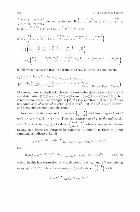
166 3 The Theory of Spinors(r1+r2 s1+s2
m1+m2 n1+n2
)defined as follows. If
1
φ, . . . ,r1+r2
φ ∈ ß,1
ψ, . . . ,s1+s2
ψ ∈
ß,1μ, . . . ,
m1+m2μ ∈ ß∗ and
1ν, . . . ,
n1+n2ν ∈ ß∗, then
(ξ ⊗ ζ)
(1
φ, . . . ,r1+r2
φ ,1
ψ, . . . ,s1+s2
ψ ,1μ, . . . ,
m1+m2μ ,
1ν, . . . ,
n1+n2ν
)
= ξ
(1
φ, . . . ,r1φ,
1
ψ, . . . ,s1
ψ,1μ, . . . ,
m1μ ,
1ν, . . . ,
n1ν
)
× ζ
(r1+1
φ , . . . ,r1+r2
φ ,s1+1
ψ , . . . ,s1+s2
ψ ,m1+1
μ , . . . ,m1+m2
μ ,n1+1
ν , . . . ,n1+n2
ν
).
It follows immediately from the definition that, in terms of components,
(ξ ⊗ ζ)A1···Ar1+r2X1···Xs1+s2B1···Bm1+m2 Y1···Yn1+n2
=(ξA1···Ar1X1···Xs1
B1···Bm1 Y1···Yn1
)(ζ
Ar1+1···Ar1+r2Xs1+1···Xs1+s2
Bm1+1···Bm1+m2 Yn1+1···Yn1+n2
).
Moreover, outer multiplication is clearly associative ((ξ⊗ζ)⊗v = ξ⊗ (ζ⊗v))and distributive (ξ⊗(ζ +v) = ξ⊗ζ +ξ⊗v and (ξ+ζ)⊗v = ξ⊗v+ζ⊗v), butis not commutative. For example, if {s1, s0} is a spin frame, then s1⊗s0 doesnot equal s0 ⊗ s1 since s1 ⊗ s0(φ∗, ψ∗) = φ1ψ0, but s0 ⊗ s1(φ∗, ψ∗) = φ0ψ1
and these are generally not the same.
Next we consider a spinor ξ of valence(
r sm n
)and two integers k and l
with 1 ≤ k ≤ r and 1 ≤ l ≤ m. Then the contraction of ξ in the indices Ak
and Bl is the spinor Ckl(ξ) of valence(
r−1 sm−1 n
)whose components relative
to any spin frame are obtained by equating Ak and Bl in those of ξ andsumming as indicated, i.e., if
ξ = ξA1···Ak···ArX1···XsB1···Bl···BmY1···Yn
sA1 ⊗ · · · ⊗ sYn ,
then
Ckl(ξ) = ξA1···A···ArX1···XsB1···A···BmY1···Yn
sA1 ⊗ · · · ⊗ sYn , (3.3.18)
where, in this last expression, it is understood that sAkand sBl are missing
in sA1 ⊗ · · · ⊗ sYn . Thus, for example, if ξ is of valence(
1 11 0
)with
ξ = ξA1X1B1
sA1 ⊗ sX1⊗ sB1

3.3 Spinor Algebra 167
and k = l = 1, then C11(ξ) is the spinor of valence(
0 10 0
)given by
C11(ξ) = ξAX1AsX1
=(ξ1X1
1 + ξ0X10
)sX1
.
Unlike our previous definitions that were coordinate-free, contractions aredefined in terms of components and so it is not immediately apparent thatwe have defined a spinor at all. We must verify that the components of Ckl(ξ)as defined by (3.3.18) transform correctly, i.e., as the components of a spinor
of valence(
r−1 sm−1 n
). But this is clearly the case since, in a new spin frame,
ξA1···A···ArX1···XsB1···A···BmY1···Yn
= GA1C1 · · · GA
Ck· · · GAr
Cr GX1U1
· · · GXsUs
GB1D1 · · ·GA
Dl · · ·
GBm
DmGY1
V1 · · · GYn
VnξC1···Ck···CrU1···UsD1···Dl···DmY1···Yn
=(GA
CkGA
Dl)GA1
C1 · · · GYn
VnξC1···Ck···CrU1···UsD1···Dl···DmY1···Yn
= δDl
CkGA1
C1 · · · GYn
VnξC1···Ck···CrU1···UsD1···Dl···DmY1···Yn
= GA1C1 · · · GYn
VnξC1···A···CrU1···UsD1···A···DmY1···Yn
.
One can, in the same way, contract a spinor ξ of valence(
r sm n
)in two
dotted indices k and l, one upper and one lower, to obtain a spinor Ckl(ξ) of
valence(
r s−1m n−1
). Observe that the processes of raising and lowering indices
discussed earlier are actually outer products (with an ε spinor) followed by acontraction.
Exercise 3.3.6 Let φ be a spinor of valence(
0 02 0
)and denote its compo-
nents in a spin frame by φAB . Show that
1. φ11 = −φ10, φ0
0 = φ01, φ10 = φ11, φ0
1 = −φ00,
2. φ11 = φ00, φ00 = φ11, φ10 = −φ01, φ01 = −φ10,
3. φABφAB = 2 det[φ11 φ10
φ01 φ00
]= 2 det
[φ1
1 φ10
φ01 φ0
0
],
4. φAC φBC =
⎧⎨⎩ 0, A = Bdet[φAB ], A = 0, B = 1
− det[φAB ], A = 1, B = 0.
Let ξ denote a spinor with the same number of dotted and undotted indices,
say, of valence[r r0 0
]. We define a new spinor denoted ξ and called the

168 3 The Theory of Spinors
conjugate of ξ by specifying that its components ξA1···ArX1···Xr in any spinframe are given by
ξA1···ArX1···Xr = ξA1···ArX1···Xr
(here we must depart from our habit of selecting dotted/undotted indicesfrom the end/beginning of the alphabet). Thus, for example, if ξ has compo-nents ξAX , then the components of ξ are given by ξ01 = ξ01, ξ11 = ξ11, etc.
Exercise 3.3.7 Show that we have actually defined a spinor of the requiredtype by verifying the appropriate transformation law, i.e.,
¯ξA1···ArX1···Xr = GA1
C1· · · GAr
CrGX1
U1 · · · GXrUr ξ
C1···CrU1···Ur .
Entirely analogous definitions and results apply regardless of the positions(upper or lower) of the indices, provided only that the number of dottedindices is the same as the number of undotted indices. We shall say thatsuch a spinor ξ is Hermitian if ξ = ξ. Thus, for example, if ξ is of va-
lence(
r r0 0
), then it is Hermitian if ξA1···ArX1···Xr = ξA1···ArX1···Xr for all
A1, . . . , Ar, X1, . . . , Xr, i.e., if
ξA1···ArX1···Xr = ξA1···ArX1···Xr ,
e.g., if r = 1, ξ01 = ξ01, ξ00 = ξ00, etc.As a multilinear functional a spinor ξ operates on four distinct types of
objects (elements of ß, ß, ß∗ and ß∗) and, if the valence is(
r sm n
), has
r + s + m + n “slots” (variables) into which these objects are inserted forevaluation, each slot corresponding to an index position in our notationfor ξ’s components. If ξ has the property that, for two such slots of thesame type, ξ(. . . , p, . . . , q, . . .) = ξ(. . . , q, . . . , p, . . .) for all p and q of theappropriate type, then ξ is said to be symmetric in these two variables (ifξ(. . . , p, . . . , q, . . .) = −ξ(. . . , q, . . . , p, . . .), it is skew-symmetric). It follows atonce from the definition that ξ is symmetric (skew-symmetric) in the vari-ables p and q if and only if the components of ξ in every spin frame areunchanged (change sign) when the corresponding indices are interchanged.We will be particularly interested in the case of spinors with just two indices.
Thus, for example, a spinor φ of valence(
0 02 0
)is symmetric (in its only two
variables) if and only if, in every spin frame, φBA = φAB for all A, B = 1, 0; φis skew-symmetric if φBA = −φAB for all A and B. On the other hand, an
arbitrary spinor ξ of valence(
0 02 0
)has a symmetrization whose components
in each spin frame are given by
ξ(AB) = 12 (ξAB + ξBA)

3.4 Spinors and World Vectors 169
and a skew-symmetrization given by
ξ[AB ] = 12(ξAB − ξBA).
The symmetrization (skew-symmetrization) of ξ clearly defines a spinor, also
of valence(
0 02 0
), that is symmetric (skew-symmetric).
Exercise 3.3.8 Let α and β be two spin vectors. The outer product α ⊗ β
is a spinor of valence(
0 02 0
)whose components in any spin frame are given
by αAβB, A, B = 1, 0. Let φ be the symmetrization of α ⊗ β so that
φAB = α(AβB) = 12(αAβB + αBβA).
Show that φAB = 12(αAβB + αBβA) and that
φABφAB = − 12
< α, β >2 .
3.4 Spinors and World Vectors
In this section we will establish a correspondence between spinors of valence(1 10 0
)and vectors in Minkowski spacetime (also called world vectors
or 4-vectors). This correspondence, which we have actually seen before(in Section 1.7), is most easily phrased in terms of the Pauli spin matrices.
Exercise 3.4.1 Let σ1 =[0 11 0
], σ2 =
[0 i−i 0
], σ3 =
[1 00 −1
], and σ4 =[
1 00 1
]. Verify the following commutation relations:
σ12 = σ2
2 = σ32 = σ4
2 = σ4,
σ1σ2 = −σ2σ1 = −iσ3,
σ1σ3 = −σ3σ1 = iσ2,
σ2σ3 = −σ3σ2 = −iσ1.
For what follows it will be convenient to introduce a factor of 1√2
and somerather peculiar looking indices, the significance of which will become clearshortly. Thus, for each A = 1, 0 and X = 1, 0, we define matrices
σaAX =
[σa
11 σa10
σa01 σa
00
], a = 1, 2, 3, 4,
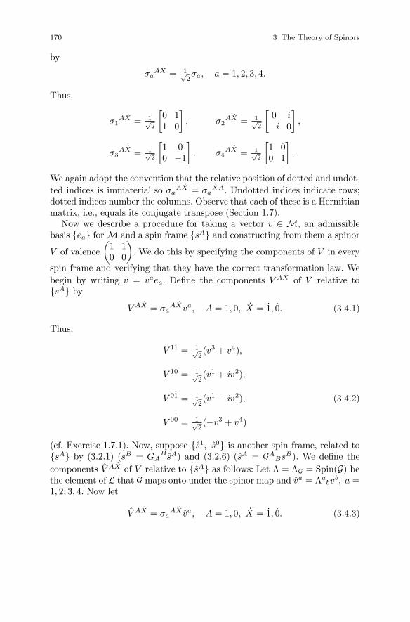
170 3 The Theory of Spinors
by
σaAX = 1√
2σa, a = 1, 2, 3, 4.
Thus,
σ1AX = 1√
2
[0 11 0
], σ2
AX = 1√2
[0 i−i 0
],
σ3AX = 1√
2
[1 00 −1
], σ4
AX = 1√2
[1 00 1
].
We again adopt the convention that the relative position of dotted and undot-ted indices is immaterial so σa
AX = σaXA. Undotted indices indicate rows;
dotted indices number the columns. Observe that each of these is a Hermitianmatrix, i.e., equals its conjugate transpose (Section 1.7).
Now we describe a procedure for taking a vector v ∈ M, an admissiblebasis {ea} for M and a spin frame {sA} and constructing from them a spinor
V of valence(
1 10 0
). We do this by specifying the components of V in every
spin frame and verifying that they have the correct transformation law. Webegin by writing v = vaea. Define the components V AX of V relative to{sA} by
V AX = σaAXva, A = 1, 0, X = 1, 0. (3.4.1)
Thus,
V 11 = 1√2(v3 + v4),
V 10 = 1√2(v1 + iv 2),
V 01 = 1√2(v1 − iv 2), (3.4.2)
V 00 = 1√2(−v3 + v4)
(cf. Exercise 1.7.1). Now, suppose {s1, s0} is another spin frame, related to{sA} by (3.2.1) (sB = GA
B sA) and (3.2.6) (sA = GABsB). We define the
components V AX of V relative to {sA} as follows: Let Λ = ΛG = Spin(G) bethe element of L that G maps onto under the spinor map and va = Λa
bvb, a =
1, 2, 3, 4. Now let
V AX = σaAX va, A = 1, 0, X = 1, 0. (3.4.3)
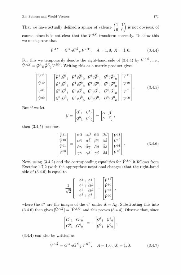
3.4 Spinors and World Vectors 171
That we have actually defined a spinor of valence(
1 10 0
)is not obvious, of
course, since it is not clear that the V AX transform correctly. To show thiswe must prove that
V AX = GABGX
Y V BY , A = 1, 0, X = 1, 0. (3.4.4)
For this we temporarily denote the right-hand side of (3.4.4) by V AX , i.e.,V AX = GA
BGXY
V BY . Writing this as a matrix product gives⎡⎢⎢⎢⎢⎢⎣V 11
V 10
V 01
V 00
⎤⎥⎥⎥⎥⎥⎦ =
⎡⎢⎢⎢⎢⎢⎣G1
1G11
G11G1
0G1
0G11
G10G1
0
G11G0
1G1
1G00
G10G0
1G1
0G00
G01G1
1G0
1G10
G00G1
1G0
0G10
G01G0
1G0
1G00
G00G0
1G0
0G00
⎤⎥⎥⎥⎥⎥⎦
⎡⎢⎢⎢⎢⎢⎣V 11
V 10
V 01
V 00
⎤⎥⎥⎥⎥⎥⎦ . (3.4.5)
But if we let
G =
[G1
1 G10
G01 G0
0
]=[α βγ δ
],
then (3.4.5) becomes⎡⎢⎢⎢⎣V 11
V 10
V 01
V 00
⎤⎥⎥⎥⎦ =
⎡⎢⎢⎢⎣αα αβ αβ ββ
αγ αδ βγ βδ
αγ βγ αδ βδ
γγ γδ γδ δδ
⎤⎥⎥⎥⎦⎡⎢⎢⎢⎣
V 11
V 10
V 01
V 00
⎤⎥⎥⎥⎦ . (3.4.6)
Now, using (3.4.2) and the corresponding equalities for V AX it follows fromExercise 1.7.2 (with the appropriate notational changes) that the right-handside of (3.4.6) is equal to
1√2
⎡⎢⎢⎣v3 + v4
v1 + iv2
v1 − iv2
−v3 + v4
⎤⎥⎥⎦ =
⎡⎢⎢⎢⎣V 11
V 10
V 01
V 00
⎤⎥⎥⎥⎦ ,
where the va are the images of the va under Λ = ΛG. Substituting this into(3.4.6) then gives [V AX ] = [V AX ] and this proves (3.4.4). Observe that, since[
G11 G1
0
G01 G0
0
]= −[G1
1 G10
G01 G0
0
],
(3.4.4) can also be written as
V AX = GABGX
Y V BY , A = 1, 0, X = 1, 0. (3.4.7)

172 3 The Theory of Spinors
We conclude then that the procedure we have described does indeed define a
spinor of valence(
1 10 0
)which we shall call the spinor equivalent of v ∈ M
(somewhat imprecisely since V depends not only on v, but also on the initialchoices of {ea} and {sA}). Observe that the conjugate V of V has componentsV AX = V AX = σa
AXva = σaAXva = σa
AXva = V AX since the matricesσa
AX are Hermitian and the va are real. Thus, the spinor equivalent of anyworld vector is a Hermitian spinor.
With (3.4.4) we can now justify the odd arrangement of indices in thesymbols σa
AX by showing that the σaAX are constant under the combined
effect of a G ∈ SL(2,C) and the corresponding Λ = ΛG in L, i.e., that
ΛabGA
BGXY
σbBY = σa
AX , a = 1, 2, 3, 4, A = 1, 0, X = 1, 0 (3.4.8)
(one might say that the σaAX are the components of a constant “spinor-
covector”). To see this we select an arbitrary admissible basis and spin frame.Fix A and X. Now let v = vaea be an arbitrary vector in M. Then V AX =σa
AXva. In another spin frame, related to the original by G, we have
V AX = σaAX va.
But also,
V AX = GAB GX
YV BY = GA
BGXY
(σb
BY vb)
= GAB GX
Yσb
BY(δbcv
c)
= GAB GX
Yσb
BY(Λa
bΛacv
c)
= ΛabGA
BGXY
σbBY (Λa
cvc)
= ΛabGA
BGXY
σbBY va.
Thus,
ΛabGA
BGXY
σbBY va = σa
AX va.
But v was arbitrary so we may successively select v’s that give (v1, v2, v3, v4)equal to (1, 0, 0, 0), (0, 1, 0, 0), (0, 0, 1, 0) and (0, 0, 0, 1) and thereby obtain(3.4.8) for a = 1, 2, 3 and 4, respectively. Since
[GA
B
]= −[GA
B
]we again
find that (3.4.8) can be written
ΛabGA
BGXY
σbBY = σa
AX , a = 1, 2, 3, 4, A = 1, 0, X = 1, 0. (3.4.9)
Exercise 3.4.2 Show that
GABGX
Yσa
BY = Λαaσα
AX , a = 1, 2, 3, 4, A = 1, 0, X = 1, 0. (3.4.10)
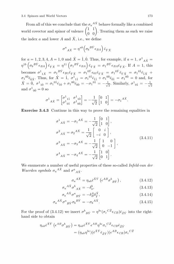
3.4 Spinors and World Vectors 173
From all of this we conclude that the σaAX behave formally like a combined
world covector and spinor of valence(
1 10 0
). Treating them as such we raise
the index a and lower A and X, i.e., we define
σaAX = ηab
(σb
BY εBA
)εY X
for a = 1, 2, 3, 4, A = 1, 0 and X = 1, 0. Thus, for example, if a = 1, σ1AX =
η1b(σb
BY εBA
)εY X = η11
(σ1
BY εBA
)εY X = σ1
BY εBAεY X . If A = 1, this
becomes σ11X = σ1
BY εB1εY X = σ10Y ε01εY X = σ1
0Y εY X = σ101ε1X +
σ100ε0X . Thus, for X = 1, σ1
11 = σ101ε11 + σ1
00ε01 = σ100 = 0 and, for
X = 0, σ110 = σ1
01 ε10 + σ100ε00 = −σ1
01 = − 1√2. Similarly, σ1
01 = − 1√2
and σ100 = 0 so
σ1AX =
[σ1
11 σ110
σ101 σ1
00
]= − 1√
2
[0 11 0
]= −σ1
AX .
Exercise 3.4.3 Continue in this way to prove the remaining equalities in
σ1AX = −σ1
AX = − 1√2
[0 11 0
],
σ2AX = σ2
AX =1√2
[0 i
−i 0
],
σ3AX = −σ3
AX = − 1√2
[1 00 −1
],
σ4AX = −σ4
AX = − 1√2
[1 00 1
].
(3.4.11)
We enumerate a number of useful properties of these so-called Infeld-van derWaerden symbols σa
AX and σaAX .
σaAX = ηab ε
XY(εABσb
BY
), (3.4.12)
σaAXσb
AX = −δba, (3.4.13)
σaAXσa
BY = −δABδX
Y, (3.4.14)
σaAXσa
BY σbBY = −σb
AX . (3.4.15)
For the proof of (3.4.12) we insert σbBY = ηbc(σc
CZεCB)εZY into the right-hand side to obtain
ηab εXY(εABσb
BY
)= ηab ε
XY εABηbcσcCZεCB εZY
= (ηabηbc)(εXY εZY )(εABεCB)σc
CZ
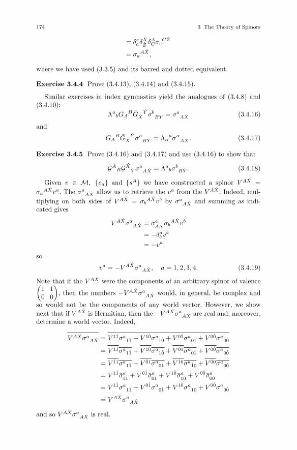
174 3 The Theory of Spinors
= δcaδX
ZδACσc
CZ
= σaAX ,
where we have used (3.3.5) and its barred and dotted equivalent.
Exercise 3.4.4 Prove (3.4.13), (3.4.14) and (3.4.15).
Similar exercises in index gymnastics yield the analogues of (3.4.8) and(3.4.10):
ΛabGA
BGXY σb
BY = σaAX (3.4.16)
and
GABGX
Y σaBY = Λα
aσαAX . (3.4.17)
Exercise 3.4.5 Prove (3.4.16) and (3.4.17) and use (3.4.16) to show that
GABGX
Y σaAX = Λa
bσbBY . (3.4.18)
Given v ∈ M, {ea} and {sA} we have constructed a spinor V AX =σa
AXva. The σaAX allow us to retrieve the va from the V AX . Indeed, mul-
tiplying on both sides of V AX = σbAXvb by σa
AX and summing as indi-cated gives
V AXσaAX = σa
AXσb
AXvb
= −δab vb
= −va,
so
va = −V AXσaAX , a = 1, 2, 3, 4. (3.4.19)
Note that if the V AX were the components of an arbitrary spinor of valence(1 10 0
), then the numbers −V AXσa
AX would, in general, be complex and
so would not be the components of any world vector. However, we shownext that if V AX is Hermitian, then the −V AXσa
AX are real and, moreover,determine a world vector. Indeed,
V AXσaAX = V 11σa
11 + V 10σa10 + V 01σa
01 + V 00σa00
= V 11σa11 + V 10σa
10 + V 01σa01 + V 00σa
00
= V 11σa11 + V 01σa
01 + V 10σa10 + V 00σa
00
= V 11σa11
+ V 01σa01
+ V 10σa10
+ V 00σa00
= V 11σa11 + V 01σa
01 + V 10σa10 + V 00σa
00
= V AXσaAX
and so V AXσaAX is real.
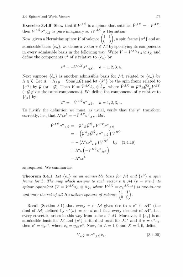
3.4 Spinors and World Vectors 175
Exercise 3.4.6 Show that if V AX is a spinor that satisfies V AX = −V AX ,then V AXσa
AX is pure imaginary so iV AX is Hermitian.
Now, given a Hermitian spinor V of valence(
1 10 0
), a spin frame {sA} and an
admissible basis {ea}, we define a vector v ∈ M by specifying its componentsin every admissible basis in the following way: Write V = V AXsA ⊗ sX anddefine the components va of v relative to {ea} by
va = −V AXσaAX , a = 1, 2, 3, 4.
Next suppose {ea} is another admissible basis for M, related to {ea} byΛ ∈ L. Let Λ = Λ±G = Spin(±G) and let {sA} be the spin frame related to{sA} by G (or −G). Then V = V AX sA ⊗ ¯sX , where V AX = GA
BGXY
V BY
(−G gives the same components). We define the components of v relative to{ea} by
va = −V AXσaAX , a = 1, 2, 3, 4.
To justify the definition we must, as usual, verify that the va transformcorrectly, i.e., that Λa
bvb = −V AXσa
AX . But
−V AXσaAX = −GA
BGXY V BY σa
AX
= −(GA
B GXY σa
AX
)V BY
= −(Λa
bσbBY
)V BY by (3.4.18)
= Λab
(−V BY σb
BY
)= Λa
bvb
as required. We summarize:
Theorem 3.4.1 Let {ea} be an admissible basis for M and {sA} a spinframe for ß. The map which assigns to each vector v ∈ M (v = vaea) itsspinor equivalent (V = V AXsA ⊗ sX , where V AX = σa
AXva) is one-to-one
and onto the set of all Hermitian spinors of valence(
1 10 0
).
Recall (Section 3.1) that every v ∈ M gives rise to a v∗ ∈ M∗ (thedual of M) defined by v∗(u) = v · u and that every element of M∗, i.e.,every covector, arises in this way from some v ∈ M. Moreover, if {ea} is anadmissible basis for M and {ea} is its dual basis for M∗ and if v = vaea,then v∗ = vaea, where va = ηaαvα. Now, for A = 1, 0 and X = 1, 0, define
VAX = σaAXva. (3.4.20)

176 3 The Theory of Spinors
Exercise 3.4.7 Show that
VAX = V BY εBAεY X , (3.4.21)
where V BY = σbBY vb.
Since V BY are the components, relative to a spin frame {sA}, of a spinor of
valence(
1 10 0
)and (3.4.21) exhibits the VAX as the result of two successive
contracted outer products of this spinor (with ε and ε), we conclude that
the VAX are the components, relative to {sA}, of a spinor of valence(
0 01 1
)which we call the spinor equivalent of the covector v∗.
Exercise 3.4.8 Show that, in another spin frame {sA} related to {sA} by(3.2.1) and (3.2.6),
VAX = σaAX va, (3.4.22)
where va = Λabvb, Λ being Λ±G .
Theorem 3.4.2 Let {ea} be an admissible basis for M and {sA} a spinframe for ß. The map which assigns to each covector v∗ ∈ M∗ (v∗ = vaea)its spinor equivalent (VAXsA ⊗ sX , where VAX = σa
AXva) is one-to-one and
onto the set of all Hermitian spinors of valence(
0 01 1
).
Exercise 3.4.9 Complete the proof of Theorem 3.4.2. �
Now, let us fix an admissible basis {ea} and a spin frame {sA}. Let v =vaea and u = uaea be in M and V = V AXsA ⊗ sX and U = UAXsA ⊗ sX thespinor equivalents of v and u. We compute UAXV AX = (σa
AXua)(σbAXvb) =
(uavb)(σaAXσb
AX) = uavb(−δa
b ) = −uava = −ηabu
bva = −u · v so
UAXV AX = −u · v. (3.4.23)
Observe that if we let
[V AX ] =
[V 11 V 10
V 01 V 00
]=
1√2
[v3 + v4 v1 + iv 2
v1 − iv2 −v3 + v4
],
then det[V AX ] = − 12v · v so
VAXV AX = 2 det[V AX ] = −v · v. (3.4.24)
Consequently, if v is null, det[V AX ] = 0 so, assuming v �= 0, [V AX ] hasrank 1.
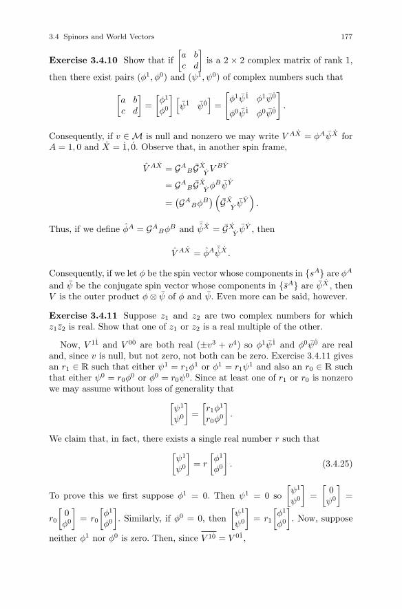
3.4 Spinors and World Vectors 177
Exercise 3.4.10 Show that if[a bc d
]is a 2 × 2 complex matrix of rank 1,
then there exist pairs (φ1, φ0) and (ψ1, ψ0) of complex numbers such that[a bc d
]=[φ1
φ0
] [ψ1 ψ0
]=
[φ1ψ1 φ1ψ0
φ0ψ1 φ0ψ0
].
Consequently, if v ∈ M is null and nonzero we may write V AX = φAψX forA = 1, 0 and X = 1, 0. Observe that, in another spin frame,
V AX = GABGX
YV BY
= GABGX
YφBψY
=(GA
BφB)(
GXY
ψY)
.
Thus, if we define φA = GABφB and ¯
ψX = GXY
ψY , then
V AX = φA ¯ψX .
Consequently, if we let φ be the spin vector whose components in {sA} are φA
and ψ be the conjugate spin vector whose components in {sA} are ψX , thenV is the outer product φ ⊗ ψ of φ and ψ. Even more can be said, however.
Exercise 3.4.11 Suppose z1 and z2 are two complex numbers for whichz1z2 is real. Show that one of z1 or z2 is a real multiple of the other.
Now, V 11 and V 00 are both real (±v3 + v4) so φ1ψ1 and φ0ψ0 are realand, since v is null, but not zero, not both can be zero. Exercise 3.4.11 givesan r1 ∈ R such that either ψ1 = r1φ
1 or φ1 = r1ψ1 and also an r0 ∈ R such
that either ψ0 = r0φ0 or φ0 = r0ψ
0. Since at least one of r1 or r0 is nonzerowe may assume without loss of generality that[
ψ1
ψ0
]=[r1φ
1
r0φ0
].
We claim that, in fact, there exists a single real number r such that[ψ1
ψ0
]= r
[φ1
φ0
]. (3.4.25)
To prove this we first suppose φ1 = 0. Then ψ1 = 0 so[ψ1
ψ0
]=[
0ψ0
]=
r0
[0φ0
]= r0
[φ1
φ0
]. Similarly, if φ0 = 0, then
[ψ1
ψ0
]= r1
[φ1
φ0
]. Now, suppose
neither φ1 nor φ0 is zero. Then, since V 10 = V 01,
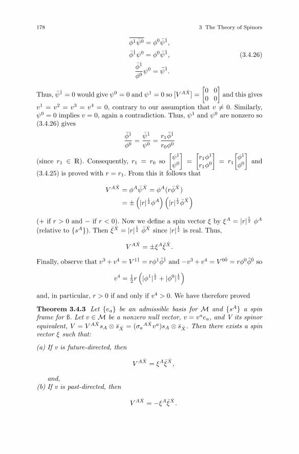
178 3 The Theory of Spinors
φ1ψ0 = φ0ψ1,
φ1ψ0 = φ0ψ1, (3.4.26)
φ1
φ0ψ0 = ψ1.
Thus, ψ1 = 0 would give ψ0 = 0 and ψ1 = 0 so [V AX ] =[0 00 0
]and this gives
v1 = v2 = v3 = v4 = 0, contrary to our assumption that v �= 0. Similarly,ψ0 = 0 implies v = 0, again a contradiction. Thus, ψ1 and ψ0 are nonzero so(3.4.26) gives
φ1
φ0=
ψ1
ψ0=
r1φ1
r0φ0
(since r1 ∈ R). Consequently, r1 = r0 so[ψ1
ψ0
]=[r1φ
1
r1φ0
]= r1
[φ1
φ0
]and
(3.4.25) is proved with r = r1. From this it follows that
V AX = φAψX = φA(rφX)
= ±(|r| 12 φA
)(|r| 12 φX
)(+ if r > 0 and − if r < 0). Now we define a spin vector ξ by ξA = |r| 12 φA
(relative to {sA}). Then ξX = |r| 12 φX since |r| 12 is real. Thus,
V AX = ±ξAξX .
Finally, observe that v3 + v4 = V 11 = rφ1φ1 and −v3 + v4 = V 00 = rφ0φ0 so
v4 = 12r(|φ1| 12 + |φ0| 12
)and, in particular, r > 0 if and only if v4 > 0. We have therefore proved
Theorem 3.4.3 Let {ea} be an admissible basis for M and {sA} a spinframe for ß. Let v ∈ M be a nonzero null vector, v = vaea, and V its spinorequivalent, V = V AXsA ⊗ sX = (σa
AXva)sA ⊗ sX . Then there exists a spinvector ξ such that:
(a) If v is future-directed, then
V AX = ξAξX ,
and,(b) If v is past-directed, then
V AX = −ξAξX .
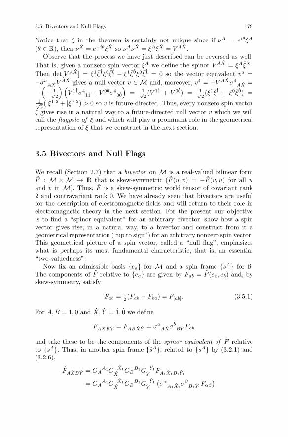
3.5 Bivectors and Null Flags 179
Notice that ξ in the theorem is certainly not unique since if νA = eiθξA
(θ ∈ R), then νX = e−iθ ξX so νAνX = ξAξX = V AX .Observe that the process we have just described can be reversed as well.
That is, given a nonzero spin vector ξA we define the spinor V AX = ξAξX .Then det[V AX ] = ξ1ξ1ξ0ξ0 − ξ1ξ0ξ0ξ1 = 0 so the vector equivalent va =−σa
AXV AX gives a null vector v ∈ M and, moreover, v4 = −V AXσ4AX =
−(− 1√
2
)(V 11σ4
11 + V 00σ400
)= 1√
2(V 11 + V 00) = 1√
2(ξ1ξ1 + ξ0ξ0) =
1√2(|ξ1|2 + |ξ0|2) > 0 so v is future-directed. Thus, every nonzero spin vector
ξ gives rise in a natural way to a future-directed null vector v which we willcall the flagpole of ξ and which will play a prominant role in the geometricalrepresentation of ξ that we construct in the next section.
3.5 Bivectors and Null Flags
We recall (Section 2.7) that a bivector on M is a real-valued bilinear formF : M × M → R that is skew-symmetric (F (u, v) = −F (v, u) for all uand v in M). Thus, F is a skew-symmetric world tensor of covariant rank2 and contravariant rank 0. We have already seen that bivectors are usefulfor the description of electromagnetic fields and will return to their role inelectromagnetic theory in the next section. For the present our objectiveis to find a “spinor equivalent” for an arbitrary bivector, show how a spinvector gives rise, in a natural way, to a bivector and construct from it ageometrical representation (“up to sign”) for an arbitrary nonzero spin vector.This geometrical picture of a spin vector, called a “null flag”, emphasizeswhat is perhaps its most fundamental characteristic, that is, an essential“two-valuedness”.
Now fix an admissible basis {ea} for M and a spin frame {sA} for ß.The components of F relative to {ea} are given by Fab = F (ea, eb) and, byskew-symmetry, satisfy
Fab = 12 (Fab − Fba) = F[ab]. (3.5.1)
For A, B = 1, 0 and X, Y = 1, 0 we define
FAXBY = FABXY = σaAXσb
BY Fab
and take these to be the components of the spinor equivalent of F relativeto {sA}. Thus, in another spin frame {sA}, related to {sA} by (3.2.1) and(3.2.6),
FAXBY = GAA1G X1
XGB
B1G Y1
YFA1X1B1Y1
= GAA1G X1
XGB
B1G Y1
Y
(σα
A1X1σβ
B1Y1Fαβ
)

180 3 The Theory of Spinors
=(GA
A1G X1
Xσα
A1X1
)(GB
B1G Y1
Yσβ
B1Y1
)Fαβ
= (Λaασa
AX)(Λb
βσbBY
)Fαβ by (3.4.17)
= σaAXσb
BY
(Λa
αΛbβFαβ
),
where Λ = ΛG . Thus,
FAXBY = σaAXσb
BY Fab . (3.5.2)
We list some useful properties of the spinor equivalent of a bivector.
Fab = σaAXσb
BY FAXBY , a, b = 1, 2, 3, 4, (3.5.3)
FAXBY = FAXBY , i.e., FAXBY is Hermitian, (3.5.4)
FBY AX = −FAXBY . (3.5.5)
The proof of (3.5.5) proceeds as follows: FBY AX = σaBY σb
AXFab =σa
BY σbAX(−Fba) = −σb
AXσaBY Fba = −σa
AXσbBY Fab = −FAXBY .
Exercise 3.5.1 Prove (3.5.3) and (3.5.4).
Now we use (3.5.5) to write
FAXBY = 12 [FAXBY − FBY AX ]
= 12[FAXBY − FBXAY + FBXAY − FBY AX ]
= 12 [FAXBY − FBXAY ] + 1
2 [FBXAY − FBY AX ].
Observe that by (3.3.14), εABεCDFCXDY =(δCAδD
B − δDA δC
B
)FCXDY =
FAXBY − FBXAY and, similarly, εXY εUV FBUAV = FBXAY − FBY AX so
FAXBY = 12εAB εCDFCXDY + 1
2εXY εUV FBUAV
= εAB
(12εCDFCXDY
)+ εXY
(12εU V FBUAV
)= εAB
(12FCX
CY
)+ εXY
(12FBUA
U)
FAXBY = εAB
(12FCX
CY
)+ εXY
(12FUB
UA
)(3.5.6)
Now define φAB by
φAB = 12FUA
UB, A, B = 1, 0.

3.5 Bivectors and Null Flags 181
Then we claim thatφBA = φAB (3.5.7)
andφXY = 1
2FCX
CY
. (3.5.8)
To prove (3.5.7) we compute
φBA = 12FUB
UA
= − 12F U
AUB by (3.5.5)
= − 12
[εU V FV A
WB εW U
]= − 1
2
[FV A
WB
(εUV εW U
)]= − 1
2
[FV A
WB
(−εUV εUW
)]= − 1
2
[FV A
WB
(−δV
W
)]= 1
2FV A
VB = φAB .
Exercise 3.5.2 Prove (3.5.8).
With this we may write (3.5.6) as
FAXBY = εAB φXY + φAB εXY . (3.5.9)
We observe next that the process which just led us from F to FAXBY toφAB can be reversed in the following sense: Given a symmetric spinor φAB
of valence(
0 02 0
)we can define FAXBY = εAB φXY + φAB εXY and obtain a
spinor of valence(
0 02 2
)which satisfies (3.5.4) since FAXBY = (FAXBY ) =
(FXAY B) = (εXY φAB + φXY εAB) = εXY φAB + φXY εAB = εAB φXY +φAB εXY = FAXBY , and (3.5.5) since FBY AX = εBAφY X + φBAεY X =(−εAB )φXY + φAB (−εXY ) = −FAXBY . Now define Fab by (3.5.3), i.e.,
Fab = σaAXσb
BY FAXBY .
Relative to another spin frame {sA}, related to {sA} by (3.2.1) and (3.2.6),FAXBY = GA
A1GXX1GB
B1GYY1FA1X1B1Y1
.
Exercise 3.5.3 Show that σaAXσb
BY FAXBY = ΛaαΛb
βFαβ , where Λ = ΛG .
Thus, defining Fab = σaAXσb
BY FAXBY , we find that the Fab transform asthe components of a bivector and we may define F : M×M → R by

182 3 The Theory of Spinors
F (u, v) = F (uaea, vbeb)
= F (ea, eb)uavb
= Fabuavb
relative to any admissible basis. Thus, every symmetric spinor φ of valence(0 02 0
)gives rise, in a natural way, to a bivector F .
Next we use the information accumulated thus far to construct a geomet-rical representation (“up to sign”) of an arbitrary nonzero spin vector ξ. Webegin, as at the end of Section 3.4, by constructing the flagpole v of ξ (thefuture-directed null vector equivalent of V AX = ξAξX). Observe that everyspin vector in the family {eiθξ : θ ∈ R} has the same flagpole as ξ since, if ξA
is replaced by eiθξA, then ξX becomes e−iθ ξX and (eiθξA)(e−iθ ξX) = ξAξX .We call eiθ the phase factor of the corresponding member of the family.
Exercise 3.5.4 Show that, conversely, if ψ is a spin vector with the sameflagpole as ξ, then ψA = eiθξA for some θ ∈ R. Hint : Write out v1, v2, v3 andv4 in terms of ξA and ψA, show that ψ1 = eiθ1ξ1 and ψ0 = eiθ0ξ0 and thenshow θ1 = θ0 + 2nπ for some n = 0,±1, . . . .
Our geometrical representation of ξ must therefore contain more than justthe flagpole if it is to distinguish spin vectors which differ only by a phasefactor. To determine this additional element in the picture we now observe
that ξ also determines a symmetric spinor φ of valence(
0 02 0
)defined by
φAB = ξAξB .
As we saw in the discussion following (3.5.9), φAB gives rise to a spinor of
valence(
0 02 2
)defined by
FAXBY = εAB φXY + φAB εXY ,
which satisfies (3.5.4) and (3.5.5) and which, in turn, determines a bivectorF given by Fab = σa
AXσbBY FAXBY , i.e.,
Fab = σaAXσb
BY (εAB ξX ξY + ξAξB εXY ). (3.5.10)
To simplify (3.5.10) we select a spin vector η which, together with ξ, form aspin frame {ξ, η} with
< η, ξ > = ξAηA = 1 = −ξAηA.
Exercise 3.5.5 Show that
ξAηB − ξBηA = εAB (3.5.11)
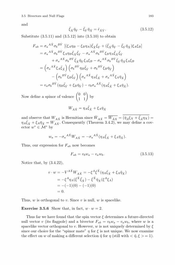
3.5 Bivectors and Null Flags 183
andξX ηY − ξY ηX = εXY . (3.5.12)
Substitute (3.5.11) and (3.5.12) into (3.5.10) to obtain
Fab = σaAXσb
BY [(ξAηB − ξBηA)ξX ξY + (ξX ηY − ξY ηX)ξAξB]
= σaAXσb
BY ξAηB ξX ξY − σaAXσb
BY ξBηAξX ξY
+ σaAXσb
BY ξX ηY ξAξB − σaAXσb
BY ξY ηXξAξB
=(σa
AXξAξX
)(σb
BY ηB ξY + σbBY ξB ηY
)−(σb
BY ξB ξY
)(σa
AXηAξX + σaAXξAηX
)= vaσb
BY (ηB ξY + ξB ηY ) − vbσaAX(ηAξX + ξAηX).
Now define a spinor of valence(
0 01 1
)by
WAX = ηAξX + ξAηX
and observe that WAX is Hermitian since WAX = WAX = (ηAξX + ξAηX) =ηAξX + ξAηX = WAX . Consequently (Theorem 3.4.2), we may define a cov-ector w∗ ∈ M∗ by
wa = −σaAXWAX = −σa
AX(ηAξX + ξAηX).
Thus, our expression for Fab now becomes
Fab = vbwa − vawb. (3.5.13)
Notice that, by (3.4.22),
v · w = −V AXWAX = −ξAξX(ηAξX + ξAηX)
= −ξAηA(ξX ξX ) − ξX ηX(ξAξA)= −(−1)(0)− (−1)(0)= 0.
Thus, w is orthogonal to v. Since v is null, w is spacelike.
Exercise 3.5.6 Show that, in fact, w · w = 2.
Thus far we have found that the spin vector ξ determines a future-directednull vector v (its flagpole) and a bivector Fab = vbwa − vawb, where w is aspacelike vector orthogonal to v. However, w is not uniquely determined by ξsince our choice for the “spinor mate” η for ξ is not unique. We now examinethe effect on w of making a different selection η for η (still with < η, ξ > = 1).

184 3 The Theory of Spinors
But < η, ξ > = < η, ξ > = 1 implies < η − η, ξ > = < η, ξ > − < η, ξ > =1 − 1 = 0 so, by (g) of Lemma 3.2.1 and the fact that ξ is not the zeroelement of ß, η − η = λξ for some λ ∈ C, i.e.,
η = η + λξ.
The new vector w is then determined by
wa = −σaAX(ηAξX + ξA
¯ηX )
= −σaAX((ηA + λξA)ξX + ξA(ηX + λξX))
= −σaAX(ηAξX + ξAηX ) − (λ + λ)σa
AXξAξX
= wa + (λ + λ)va,
Fig. 3.5.1
sow = w + (λ + λ)v. (3.5.14)
It follows that w lies in the 2-dimensional plane spanned by v and w and isa spacelike vector orthogonal to v (again, w · w = 2). Thus, ξ uniquely de-termines a future-directed null vector v and a 2-dimensional plane spannedby v and any of the spacelike vectors w, w, . . . determined by (3.5.14). This2-dimensional plane lies in the 3-dimensional subspace (Span{v})⊥, which istangent to the null cone along v. In a 3-dimensional picture, the null coneand (Span{v})⊥ appear 2-dimensional so this 2-dimensional plane is a line.However, to stress its 2-dimensionality we shall draw it as a “flag” along vas in Figure 3.5.1. The pair consisting of v and this 2-dimensional plane in

3.5 Bivectors and Null Flags 185
(Span{v})⊥ is called the null flag of ξ and is, we claim, an accurate geomet-rical representation of ξ “up to sign”. To see this we examine the effect of aphase change
ξA −→ eiθξA (θ ∈ R).
Of course, the flagpole v is unchanged, but ξX → e−iθ ξX so Fab →σa
AXσbBY (e−2θiεAB ξX ξY + e2θiξAξB εXY ). A spinor mate for eiθξA must
have the property that its ß-inner product with eiθξA is 1. Since dim ß = 2,it must be of the form
e−iθηA + kξA
for some k ∈ C. Thus,
wa −→ −σaAX [(e−iθηA + kξA)(e−iθ ξX) + (eiθξA)(eiθηX + kξX)]
= −σaAX [e−2θiηAξX + ke−iθξAξX + e2θiξAηX + keiθξAξX ]
= −σaAX(e2θiξAηX + e−2θiηAξX) − (ke−iθ + keiθ)(σa
AXξAξX)
= −σaAX [(cos 2θ + i sin 2θ)ξAηX + (cos 2θ − i sin 2θ)ηAξX ] + rva
= cos 2θ(−σa
AX(ξAηX + ηAξX))
+ sin 2θ(−σa
AX i(ξAηXηAξX))
+ rva,
where r = ke−iθ + keiθ = ke−iθ + (ke−iθ) ∈ R. Now, −σaAX(ξAηX+ηAξX) =
wa. Moreover, observe that if UAX = ξAηX − ηAξX , then UAX = −UAX
so, by Exercise 3.4.6, iU AX is Hermitian and therefore, by Theorem 3.4.2,ua = −σa
AX iU AX defines a covector u∗ in M∗. Thus, wa → wa cos 2θ +ua sin 2θ + rva so the phase change ξA → eiθξA leaves v alone and gives anew w of
w −→ (cos 2θ)w + (sin 2θ)u + rv .
Exercise 3.5.7 Compute waua, vaua and uaua to show that u is orthogonalto w and v and satisfies u · u = 2.
Thus, we picture w and u as perpendicular spacelike vectors in the 3-space(Span{v})⊥ tangent to the null cone along v. Then (cos 2θ)w + (sin 2θ)uis a spacelike vector in the plane of w and u making an angle of 2θ withw. After a phase change ξA → eiθξA the new w is in the plane of v and(cos 2θ)w+(sin 2θ)u. The 2-plane containing v and this new w is the new flag.Thus, a phase change ξA → eiθξA leaves the flagpole v unchanged and rotatesthe flag by 2θ in the plane of w and u (in Figure 3.5.2 we have drawn theflagpole vertically even though it lies along a null line). Notice that if θ = π,then the phase change ξA → eπiξA = −ξA carries ξ to −ξ, but the null flagis rotated by 2π and so returns to its original position. Thus, ξ determines aunique null flag, but the null flag representing ξ also represents −ξ. Hence,null flags represent spin vectors only “up to sign”. This is a reflection of whatmight be called the “essential 2-valuedness” of spinors, which has its roots in
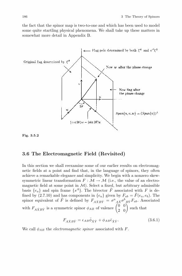
186 3 The Theory of Spinors
the fact that the spinor map is two-to-one and which has been used to modelsome quite startling physical phenomena. We shall take up these matters insomewhat more detail in Appendix B.
Fig. 3.5.2
3.6 The Electromagnetic Field (Revisited)
In this section we shall reexamine some of our earlier results on electromag-netic fields at a point and find that, in the language of spinors, they oftenachieve a remarkable elegance and simplicity. We begin with a nonzero skew-symmetric linear transformation F : M → M (i.e., the value of an electro-magnetic field at some point in M). Select a fixed, but arbitrary admissiblebasis {ea} and spin frame {sA}. The bivector F associated with F is de-fined by (2.7.10) and has components in {ea} given by Fab = F (ea, eb). Thespinor equivalent of F is defined by FAXBY = σa
AXσbBY Fab . Associated
with FAXBY is a symmetric spinor φAB of valence(
0 02 0
)such that
FAXBY = εAB φXY + φAB εXY . (3.6.1)
We call φAB the electromagnetic spinor associated with F .

3.6 The Electromagnetic Field (Revisited) 187
Exercise 3.6.1 Show that if ξ is any spin vector, then φABξAξB is an in-variant, i.e., that, relative to another spin frame,
φAB ξAξB = φABξAξB .
Our first objective is to obtain a canonical decomposition of φAB intoa symmetrized outer product of spin vectors. To this end we compute the
invariant in Exercise 3.6.1 for spin vectors of the form[ξ1
ξ0
]=[z1
], where
z ∈ C.
φABξAξB = φ11ξ1ξ1 + φ10ξ
1ξ0 + φ01ξ0ξ1 + φ00ξ
0ξ0
= φ11z2 + φ10z + φ01z + φ00
= φ11z2 + 2φ10z + φ00
since φ01 = φ10. Notice that this is a quadratic polynomial in the complexvariable z with coefficients in C. Consequently, it factors over C, i.e., thereexist α1, α0, β1, β0 ∈ C such that
φ11z2 + 2φ10z + φ00 = (α1z + α0)(β1z + β0) (3.6.2)
(these are not unique, of course, since replacing αA by αA/γ and βA by γβA
for any nonzero γ ∈ C also gives a factorization). Equating coefficients in(3.6.2) gives
φ11 = α1β1 = 12 (α1β1 + α1β1)
φ00 = α0β0 = 12 (α0β0 + α0β0)
φ10 = 12(α1β0 + α0β1).
Since φ01 = φ10 this last equality may be written
φ01 = 12 (α0β1 + α1β0).
Thus, for all A, B = 1, 0, we have
φAB = 12 (αAβB + αBβA). (3.6.3)
Next observe that if, in another spin frame, we define αA = GAA1αA1 and
βB = GBB1βB1 , i.e., if we regard α and β as spin vectors, then
188 3 The Theory of Spinors
12(αAβB + αB βA) = 1
2
((GA
A1αA1
) (GB
B1βB1
)+(GB
B1αB1
) (GA
A1αA1
))= 1
2GA
A1GBB1(αA1βB1 + αB1βA1)
= GAA1GB
B1φA1B1
= φAB .
Consequently, φ is the symmetrized outer product of the spin vectors α andβ, i.e., in any spin frame,
φAB = 12(αAβB + αBβA) = α(AβB). (3.6.4)
Although we will have no need to do so this argument, which depends onlyon the symmetry of φ, extends easily to produce analogous decompositionsof higher valence symmetric spinors.
The spin vectors α and β are intimately connected with the electromag-netic field F . We will eventually show that our characterization of null andregular F ’s (Corollary 2.3.8) has a remarkably simple reformulation in termsof α and β (Corollary 3.6.2 asserts that F is null if and only if α and β areparallel). For the present we will content ourselves with showing that thefuture-directed null vectors associated with α and β (i.e., their flagpoles) areeigenvectors of the electromagnetic field F (see Section 2.4). Thus, we definefuture-directed null vectors v and w by
va = −σaAXαAαX and wa = −σa
AXβAβX .
The null directions determined by v and w are called the principal null di-rections of φAB . Letting F a
b = ηacFcb denote the entries in the matrix of Frelative to {ea} we compute
F abv
b = ηacFcbvb = ηacσc
AXσbBY FAXBY vb
= −ηacσcAXσb
BY (εAB φXY + φAB εXY )(σb
DZαDαZ)
= −ηacσcAX(σb
BY σbDZ
)(εAB φXY + φAB εXY )αDαZ
= −ηacσcAX(−δB
DδYZ
)(εAB φXY + φAB εXY )αDαZ
= ηacσcAX(εAB φXY + φAB εXY )αBαY
= ηacσcAX[(εABαB)(φXY αY ) + (φABαB)(εXY αY )
]F a
bvb = ηacσc
AX[(−αA)(φXY αY ) + (φABαB)(−αX)
]. (3.6.5)

3.6 The Electromagnetic Field (Revisited) 189
Exercise 3.6.2 Show that φABαB = 12(α1β0 − α0β1)αA and φXY αY =
12(α1β0 − α0β1)αX .
Letting μ = 12(α1β0 − α0β1) we obtain, from Exercise 3.6.2,
φABαB = μαA (3.6.6)
and
φXY αY = μαX , (3.6.7)
which we now substitute into (3.6.5).
F abv
b = −ηacσcAX(αA(μαX) + (μαA)αX )
= −ηacσcAX(μ + μ)(αAαX)
= −(μ + μ)ηac(σcAXαAαX)
= −(μ + μ)ηacvc
= −(μ + μ)va.
If we let
λ = −(μ + μ) = −2Re(μ) = −2Re(
12(α1β0 − α0β1)
)= −Re(α1β0 − α0β1)= −Re < α, β >,
we obtainF a
bvb = λva = −Re < α, β > va, (3.6.8)
or, equivalently,Fv = λv = −Re < α, β > v, (3.6.9)
so v is an eigenvector of F with eigenvalue λ = −Re < α, β >.
Exercise 3.6.3 Show in the same way that
Fw = −λw = Re < α, β > w. (3.6.10)
We conclude that the flagpoles of α and β are two (possibly coincident)future-directed null eigenvectors of F with eigenvalues −Re < α, β > andRe < α, β > respectively.
Let us rearrange (3.6.6) a bit.
φAC αC = μαA,
φAC (εCBαB) = μαA,
(φAC εCB)αB = μαA,
(−εBCφAC )αB = μαA,
φABαB = −μαA. (3.6.11)
190 3 The Theory of Spinors
Thinking of[φA
B
]as the matrix, relative to {sA}, of a linear transformation
φ : ß → ß on spin space motivates the following definitions. A complex numberλ is an eigenvalue of φAB if there exists a nonzero spin vector α ∈ ß, calledan eigenspinor of φAB , such that φA
BαB = λαA. Such an α will exist if andonly if λ satisfies
det[[
φ11 φ1
0
φ01 φ0
0
]− λ
[1 00 1
]]= 0,
which, when expanded, gives
λ2 −(φ1
1 + φ00)
+ det[φA
B]
= 0. (3.6.12)
However, #1 of Exercise 3.3.6 and the symmetry of φAB gives φ11 +φ0
0 = 0,whereas #3 of that same Exercise gives det
[φA
B]
= det [φAB ] = 12φABφAB ,
so the solutions to (3.6.12) are
λ = ±(− det[φAB ])12 = ±
(− 1
2φABφAB
) 12 . (3.6.13)
The physical significance of these eigenvalues of φAB will emerge when wecompute det[φAB ] in terms of the 3-vectors
⇀
E and⇀
B, which we accomplishby means of (2.7.14). First observe that
φAB = 12FUA
UB = 1
2
[F1A
1B + F0A
0B
]= 1
2
[ε1XF1AXB + ε0XF0AXB
]= 1
2
[ε10F1A0B + ε01F0A1B
]= 1
2[−F1A0B + F0A1B] = 1
2[FA0B1 − FA1B0].
Thus, for example,
φ11 = 12 [F1011 − F1110] = 1
2 [F1011 − (−F1011)]
= F1011 = σa10σ
b11Fab .
Now, if a = b the corresponding term in this sum is zero since Faa = 0. Thea = 3, 4 and b = 1, 2 terms vanish by the definitions of the σa
AX . Thus, onlythe ab = 13, 14, 23, 24 terms survive so

3.6 The Electromagnetic Field (Revisited) 191
φ11 = σ110σ
311F13 + σ1
10σ411F14 + σ2
10σ311F23 + σ2
10σ411F24
=(− 1√
2
)(− 1√
2
)F13 +
(− 1√
2
)(− 1√
2
)F14
+(
i√2
)(− 1√
2
)F23 +
(i√2
)(− 1√
2
)F24
= 12(−B2) + 1
2(E1) − 1
2i(B1) − 1
2i(E2)
φ11 = 12 [(E1 − B2) − i(E2 + B1)]. (3.6.14)
Exercise 3.6.4 Continue in the same way to show
φ10 = φ01 = 12 (−E3 + iB3) (3.6.15)
and
φ00 = 12 [−(E1 + B2) + i(−E2 + B1)]. (3.6.16)
Exercise 3.6.5 Compute φ11φ00–φ10φ01 from (3.6.14)–(3.6.16) to show that
det[φAB ] = 14
(|⇀
B|2 − |⇀
E|2)
+ 12(
⇀
E ·⇀
B)i. (3.6.17)
Returning now to (3.6.13) we find that the eigenvalues of the electromagneticspinor φAB are given by
λ = ±[− 1
4(|
⇀
B|2 − |⇀
E|2) − 12(⇀
E ·⇀
B)i] 1
2. (3.6.18)
But then λ = 0 if and only if |⇀
B|2 − |⇀
E|2 =⇀
E ·⇀
B = 0 so F is null if and onlyif the only eigenvalue of φAB is 0 and we have proved:
Theorem 3.6.1 Let F : M → M be a nonzero, skew-symmetric lineartransformation, F its associated bivector, FAXBY the spinor equivalent ofF and φAB the symmetric spinor for which FAXBY = εAB φXY + φAB εXY .Then F is null if and only if λ = 0 is the only eigenvalue of φAB .
Another equally elegant form of this characterization theorem is:
Corollary 3.6.2 Let F : M → M be a nonzero, skew-symmetric lineartransformation, F its associated bivector, FAXBY the spinor equivalent ofF , φAB the symmetric spinor for which FAXBY = εAB φXY + φAB εXY , andα and β spin vectors for which φAB = α(AβB). Then F is null if and only ifα and β are linearly dependent.

192 3 The Theory of Spinors
Proof: First we compute
φABφAB = 12 (αAβB + αBβA) 1
2
(αAβB + αBβA
)= 1
4
[(αAαA
) (βBβB
)+(αAβA
) (βBαB
)+(αBβB
) (βAαA
)+(αBαB
) (βAβA
)]= 1
4 [(0)(0)+ < β, α > < α, β > + < β, α > < α, β > + (0)(0)]
= 14[− < α, β > < α, β > − < α, β > < α, β >]
= − 12
< α, β >2 .
Thus, (3.6.13) gives
λ = ±(
14 < α, β >2
) 12 = ± 1
2 < α, β > .
Theorem 3.6.1 therefore implies that F is null if and only if < α, β > = 0which, by Lemma 3.2.1 (g), is the case if and only if α and β are linearlydependent. �
We have defined the spinor equivalent of a bivector in Section 3.5, butthe same definition yields a spinor equivalent of any bilinear form on M.Specifically, if we fix an admissible basis {ea} and a spin frame {sA} and letH : M×M → R be a bilinear form on M, then the spinor equivalent of H
is the spinor of valence(
0 02 2
)whose components in {sA} are given by
HAXBY = σaAXσb
BY Hab ,
where Hab = H(ea, eb).
Exercise 3.6.6 Show that, in another spin frame {sA}, related to {sA} by(3.2.1) and (3.2.6), HAXBY = σa
AXσbBY Hab , where Hab = Λa
αΛbβHαβ , Λ
being ΛG .
A particularly important example of a bilinear form is the Lorentz innerproduct itself: g : M×M → R, defined by g(u, v) = u · v. Relative to any{ea}, the components of g are
g(ea, eb) = ea · eb = ηab .
The spinor equivalent of g is defined by
gAXBY = σaAXσb
BY ηab
gAXBY = σ1AXσ1
BY + σ2AXσ2
BY + σ3AXσ3
BY − σ4AXσ4
BY . (3.6.19)

3.6 The Electromagnetic Field (Revisited) 193
We claim thatgAXBY = −εAB εXY . (3.6.20)
One verifies (3.6.20) by simply considering all possible choices for A, B, Xand Y . For example, if either (i) A and B are the same, but X and Y aredifferent, or (ii) X and Y are the same, but A and B are different, thenboth sides of (3.6.20) are zero (every σa
AX has either σa11 = σa
00 = 0 orσa
10 = σa01 = 0, so all of the σa
AXσaBY in (3.6.19) are zero). All that
remain then are the cases in which (iii) A = B and X = Y , or (iv) A �= Band X �= Y , i.e., AXBY = 1111, 1010, 0101, 0000, 1100, 1001, 0110, 0011.For example,
g1001 = σ110σ
101 + σ2
10σ201 + σ3
10σ301 − σ4
10σ401
= σ110σ
101 + σ2
10σ201 =
(− 1√
2
)(− 1√
2
)+(
i√2
)(− i√
2
)= 1
2 − 12 i2 = 1
2 + 12
= 1
= −ε10ε01.
Exercise 3.6.7 Verify the remaining cases.
The energy-momentum transformation T : M → M of an electromagneticfield F : M → M also has an associated (symmetric) bilinear form T :M×M → R defined by T (u, v) = u·Tv and with components Tab = T (ea, eb)given, according to Exercise 2.7.8, by
Tab = 14π
[FaαFb
α − 14ηabFαβFαβ
]. (3.6.21)
We show next that the spinor equivalent of T takes the following particularlysimple form:
TAXBY = 12π
φAB φXY , (3.6.22)
where φAB is the electromagnetic spinor associated with F . By definition,the spinor equivalent of T is given by
TAXBY = σaAXσb
BY Tab = 14π
σaAXσb
BY
[FaαFb
α − 14ηabFαβFαβ
]= 1
4π
[σa
AXσbBY FaαFb
α − 14
(σa
AXσbBY ηab
)FαβFαβ
]TAXBY = 1
4π
[σa
AXσbBY FaαFb
α + 14εAB εXY (FαβFαβ)
](3.6.23)
by (3.6.20). We begin simplifying (3.6.23) with two observations:
FαβFαβ = FCZDW FCZDW (3.6.24)
194 3 The Theory of Spinors
and
σaAXσb
BY FaαFbα = −FAXCZFBY
CZ . (3.6.25)
For the proof of (3.6.24) we compute
FCZDW FCZDW = FCZDW εCC1 εZZ1εDD1 εWW1FC1Z1D1W1
=(σa
CZσbDW Fab
)εCC 1 εZZ1εDD1 εWW1
(σα
C1Z1σβ
D1W1(ηαμηβνFμν)
)=(εCC1 εZZ1ημασα
C1Z1
)(εDD1 εWW1ηνβσβ
D1W1
)σa
CZσbDW FabF
μν
= σμCZσν
DW σaCZσb
DW FabFμν =
(σμ
CZσaCZ
)(σν
DW σbDW
)FabF
μν
=(−δa
μ
) (−δb
ν
)FabF
μν = FabFab .
Exercise 3.6.8 Prove (3.6.25).Substituting (3.6.24) and (3.6.25) into (3.6.23) gives
TAXBY = 14π
[−FAXCZFBY
CZ + 14 εAB εXY FCZDW FCZDW
]. (3.6.26)
Now we claim that if FAXBY = εAB φXY + φAB εXY , then
FCZDW FCZDW = 2(φCDφCD + φZW φZW
)(3.6.27)
and
FAXCZFBYCZ = −2φAB φXY + εAB φXZ φY
Z + εXY φAC φBC . (3.6.28)
We prove (3.6.27) as follows:
FCZDW FCZDW =(εCD φZW + φCD εZW
) (εCD φZW + φCD εZW
)=(εCDεCD
) (φZW φZW
)+(εCDφCD
) (φZW εZW
)+(φCDεCD
) (εZW φZW
)+(φCDφCD
) (εZW εZW
).
But observe that, by symmetry of φ, εCDφCD = ε10φ10 + ε01φ
01 = −φ10 +φ01 = 0 and, similarly, εZW φZW = 0. Moreover, by (3.3.7), εCDεCD =εZW εZW = 2 so
FCZDW FCZDW = 2φZW φZW + 0 + 0 + 2φCDφCD
which gives (3.6.27).

3.6 The Electromagnetic Field (Revisited) 195
Exercise 3.6.9 Prove (3.6.28).
With (3.6.27) and (3.6.28), (3.6.26) becomes
TAXBY = 14π
[2φAB φXY − εAB φXZ φY
Z − εXY φAC φBC
+ 12εAB εXY
(φCDφCD + φZW φZW
)].
TAXBY = 14π
[2φAB φXY − εAB φXZ φY
Z − εXY φAC φBC
+ (det[φAB ])εAB εXY + (det[φXY ])εAB εXY
], (3.6.29)
where we have appealed to part (3) of Exercise 3.3.6 and its conjugated ver-sion. For the remaining simplifications we use part (4) of this same exercise.If either A = B or X = Y all the terms on the right-hand side of (3.6.29)except the first are zero so TAXBY = 1
2π φAB φXY and (3.6.22) is proved. Theremaining cases are AXBY = 1100, 1001, 0110 and 0011 and all are treatedin the same way, e.g.,
T1100 = 14π
[2φ10φ10 − ε10φ1Z φ0
Z − ε10φ1Cφ0C
+ (det[φAB ])ε10ε10 + (det[φXY ])ε10ε10]
= 14π
[2φ10φ10 − (−1)(− det[φXY ]) − (−1)(− det[φAB ])+ (det[φAB ])(−1)(−1) + (det[φXY ])(−1)(−1)]
= 14π [2φ10φ10]
= 12π
φ10φ10.
Exercise 3.6.10 Check the remaining cases to complete the proof of(3.6.22).
We use the spinor equivalent TAXBY = 12π
φAB φXY of the energy-momentum T of F to give another proof of the dominant energy condition(Exercise 2.5.6) that does not depend on the canonical forms of F . Beginwith two future-directed null vectors u = uaea and v = vbeb in M. By The-orem 3.4.3, the spinor equivalents of u and v can be written UAX = μAμX
and V AX = νAνX , where μ and ν are two spin vectors. Thus, we may writeua = −σa
AXμAμX and vb = −σbBY νB νY so that
Tu · v = Tabuavb = Tab
(−σa
AXμAμX)(
−σBBY νB νY
)=(σa
AXσbBY Tab
)μAμXνB νY
= TAXBY μAμXνB νY
= 12π φAB φXY μAμXνB νY
= 12π (φABμAμB)(φXY μX νY ),

196 3 The Theory of Spinors
soTu · v = 1
2π |φABμAνB|2. (3.6.30)
In particular, Tu · v ≥ 0.
Exercise 3.6.11 Show that Tu ·v ≥ 0 whenever u and v are timelike or nulland both are future-directed. Hint : Any future-directed timelike vector canbe written as a sum of two future-directed null vectors.
We recall from Section 2.5 that, for any future-directed unit timelike vectorU, TU · U = 1
8π [|⇀
E|2 + |⇀
B|2] is the energy density in any admissible framewith e4 = U . Consequently, if F is nonzero, Tu · u �= 0 for any timelikevector u. We now investigate the circumstances under which Tv · v = 0 forsome future-directed null vector v. Suppose then that v is null and future-directed and Tv · v = 0. Write va = −σa
AXνAνX for some spin vector ν
(Theorem 3.4.3). Then, by (3.6.30), φABνAνB = 0. Using the decomposition(3.6.4) of φ this is equivalent to
(αAβB + αBβA)(νAνB) = 0,
(αAνA)(βBνB) + (αBνB)(βAνA) = 0,
2 < ν, α > < ν, β > = 0
which is the case if and only if either < ν, α > = 0 or < ν, β > = 0. But< ν, α > = 0 if and only if ν is a multiple of α (Lemma 3.2.1(g)) and similarlyfor < ν, β > = 0. But if ν is a multiple of either α or β, then v is a multiple ofone of the two null vectors determined by α or β, i.e., v is along a principalnull direction of φAB . Thus, a future-directed null vector v for which Tv ·v = 0must lie along a principal null direction of φAB . Moreover, by reversing thesteps above, one finds that the converse is also true so we have proved that anonzero null vector v satisfies Tv · v = 0 if and only if v lies along a principalnull direction of φAB .
Exercise 3.6.12 Let F : M → M be a nonzero, skew-symmetric lineartransformation, F the associated bivector and ∗F the dual of F (Section 2.7).By (2.7.16) (with M = Λ), the Levi-Civita symbol εabcd defines a (con-stant) covariant world tensor of rank 4. We define its spinor equivalent byεAXBY CZDW = σa
AXσbBY σc
CZσdDW εabcd . Show that
εAXBY CZDW = i(εAC εBD εXW εY Z − εADεBC εXZ εY W )
and then raise indices to obtain
εAXBYCZDW = i
(δCAδD
B δWX
δZY− δD
A δCBδZ
XδWY
).
Now show that the spinor equivalent of ∗F is given by
∗FAXBY = i(εAB φXY − φAB εXY ).

3.6 The Electromagnetic Field (Revisited) 197
Exercise 3.6.13 Define the spinor equivalent of an arbitrary world tensor(Section 3.1) of contravariant rank r and covariant rank s, being sure to verifythe appropriate transformation law, and show that any such spinor equivalentis Hermitian. Find an “inversion formula” analogous to (3.4.19) and (3.5.3)that retrieves the world tensor from its spinor equivalent. For what type ofspinor can this process be reversed to yield a world tensor equivalent?
We conclude our discussion of electromagnetic theory by deriving the el-egant spinor form of the source-free Maxwell equations. For this we fix anadmissible basis {ea} and a spin frame {sA} and let F denote an electro-magnetic field on (a region in) M. As usual, we denote by Fab = ηaαFα
b
the components of the corresponding bivector F , all of which are functions of(x1, x2, x3, x4). Then the spinor equivalent of F is FAXBY = σa
AXσbBY Fab
and the electromagnetic spinor φAB is given by
φAB = 12FUA
UB
= 12[FA0B1 − FA1B0].
Next we introduce “spinor equivalents” for the differential operators ∂a =∂
∂xa , a = 1, 2, 3, 4. Specifically, we define, for each A = 1, 0 and X = 1, 0, anoperator ∇AX by
∇AX = σaAX∂a = σa
AX(ηaα∂α).
Thus, for example,
∇11 = σa11∂a = σ1
11∂1 + σ211∂2 + σ3
11∂3 + σ411∂4
= σ311∂3 + σ4
11∂4 = 1√2∂3 + 1√
2∂4
= 1√2(∂3 − ∂4).
Exercise 3.6.14 Prove the remaining identities in (3.6.31):
∇11 = 1√2(∂3 − ∂4), ∇10 = 1√
2(∂1 + i∂2),
∇01 = 1√2(∂1 − i∂2), ∇00 = − 1√
2(∂3 + ∂4).
(3.6.31)
With this notation we claim that all of the information contained in thesource-free Maxwell equations (2.7.15) and (2.7.21) can be written con-cisely as
∇AXφAB = 0, A = 1, 0, X = 1, 0. (3.6.32)
Equations (3.6.32) are the spinor form of the source-free Maxwell equations.To verify the claim we write
φ11 = 12 [(F13 + F14) + i(F32 + F42)],
φ10 = φ01 = 12 [F43 + iF 12],
φ00 = 12 [(F41 + F13) + i(F42 + F23)]

198 3 The Theory of Spinors
(see (3.6.14)–(3.6.16)). Now compute, for example,
∇A1φA0 = ∇11φ10 + ∇01φ00 = 12√
2{(∂3 − ∂4)(F43 + iF 12)
+ (∂1 − i∂2)((F41 + F13) + i(F42 + F23))}= 1
2√
2{[−(F14,1 + F24,2 + F34,3) + (F13,1 + F23,2 − F43,4)]
+ i[(F12,3 + F31,2 + F23,1) − (F12,4 + F41,2 + F24,1)]}
= 12√
2
{[−div
⇀
E −[(curl
⇀
B) · e3 − ∂E3
∂x4
]]+ i[div
⇀
B −[(curl
⇀
E) · e3 + ∂B3
∂x4
]]}.
Exercise 3.6.15 Calculate, in the same way, ∇A1φA1, ∇A0φA1, and∇A0φA0, and show that (3.6.32) is equivalent to Maxwell’s equations.
Generalizations of (3.6.32) are used in relativistic quantum mechanics asfield equations for various types of massless particles. Specifically, if n is a
positive integer and φA1A2···An is a symmetric spinor of valence(
0 0n 0
), then
∇AXφAA2···An = 0, A2, . . . , An = 1, 0, X = 1, 0,
is taken to be the massless free-field equation for arbitrary spin 12n particles
(see 5.7 of [PR]). In particular, if n = 1, then φA is a spin vector and oneobtains the Weyl neutrino equation
∇AXφA = 0, X = 1, 0,
which suggested the possibility of parity nonconservation in weak interactionsyears before the phenomenon itself was observed (see [LY]).
Chapter 4
Prologue and Epilogue: The de SitterUniverse
4.1 Introduction
In this final chapter we would like to take one small step beyond the specialtheory of relativity in order to briefly address two issues that have been con-scientiously swept under the rug to this point. These are related, althoughperhaps not obviously so. The first is the issue of gravitation which we quiteexplicitly eliminated from consideration very early on. We have proposedMinkowski spacetime as a model of the event world only when the effects ofgravity are “negligible”, that is, for a universe that is effectively “empty”, butit is doubtful that anything in our development has made it clear why such arestriction was necessary. Here we will attempt to provide an explanation aswell as a gentle prologue to how one adapts to the presence of gravitationalfields. Then, as an epilogue to our story, we will confront certain recent astro-nomical observations suggesting that, even in an empty universe, the eventworld may possess properties not reflected in the structure of Minkowskispacetime, at least on the cosmological scale. Remarkably, there is a viablealternative, nearly 100 years old, that has precisely these properties and wewill devote a little time to becoming acquainted with it.
4.2 Gravitation
An electromagnetic field is a 2-form on Minkowski spacetime M that satisfiesMaxwell’s equations. A charged particle responds to the presence of such afield by experiencing changes in 4-momentum specified by the Lorentz 4-ForceLaw. This is how particle mechanics works. A physical agency that affects theshape of a particle’s worldline is isolated and described mathematically andthen equations of motion are postulated that quantify this effect. It wouldseem then that the next logical step in such a program would be to carry
, : An Introduction , Applied Mathematical Sciences 92,
G.L. Naber The Geometry of Minkowski Spacetime to the Mathematics of the Special Theory of RelativityDOI 10.1007/978-1-4419-7838-7_4, © Springer Science+Business Media, LLC 2012
199
200 4 Prologue and Epilogue: The de Sitter Universe
out an analogous procedure for the gravitational field. In the early days ofrelativity theory many attempts were made (by Einstein and others) to dojust this, but they all came to naught. However one chose to model a gravi-tational field on M and however the corresponding equations of motion werechosen, the numbers simply did not come out right; theoretical predictionsdid not agree with the experimental facts (an account of some of these earlyattempts is available in Chapter 2 of [MTW]). In hindsight, the reason forthese failures appears quite simple (once it is pointed out to you by Einstein,that is). An electromagnetic field is something “external” to the structure ofspacetime, an additional field defined on and (apparently) not influencing themathematical structure of M. Einstein realized that a gravitational field hasa very special property which makes it unnatural to regard it as somethingexternal to the nature of the event world. Since Galileo it has been knownthat all objects with the same initial position and velocity respond to a givengravitational field in the same way (i.e., have identical worldlines) regardlessof their material constitution (mass, charge, etc.). This is essentially whatwas verified at the Leaning Tower of Pisa and contrasts markedly with thebehavior of electromagnetic fields. These worldlines (of particles with giveninitial conditions of motion) seem almost to be natural “grooves” in space-time that anything will slide along once placed there. But these “grooves”depend on the particular gravitational field being modeled and, in any case,M simply is not “grooved” (its structure does not distinguish any collectionof curved worldlines). One suspects then that M itself is somehow lacking,that the appropriate mathematical structure for the event world may be morecomplex when gravitational effects are nonnegligible.
To see how the structure of M might be generalized to accommodate thepresence of gravitational fields let us begin again as we did in the Introductionwith an abstract set M whose elements we call “events”. One thing at least isclear. In regions that are distant from the source of any gravitational field noaccommodation is necessary and M must locally “look like” M. But a greatdeal more is true. In his now famous Elevator Experiment Einstein observedthat any event has about it a sufficiently small region of M which “lookslike” M. To see this we reason as follows. Imagine an elevator containing anobserver and various other objects that is under the influence of some uniformexternal gravitational field. The cable snaps. The contents of the elevator arenow in free fall. Since all of the objects inside respond to the gravitationalfield in the same way they will remain at relative rest throughout the fall.Indeed, if our observer lifts an apple from the floor and releases it in mid-airit will appear to him to remain stationary. You have witnessed these thingsfor yourself. While it is unlikely that you have had the misfortune of seeing afalling elevator you have seen astronauts at play inside their space capsuleswhile in orbit (i.e., free fall) about the earth. The objects inside the elevator(capsule) seem then to constitute an archetypical inertial frame. By estab-lishing spacetime coordinates in the usual way our observer thereby becomesan admissible observer, at least within the spatial and temporal constraints
4.2 Gravitation 201
imposed by his circumstances. Now, picture an arbitrary event. There are anynumber of vantage points from which the event can be observed. One is froma freely falling elevator in the immediate spatial and temporal vicinity of theevent and from this vantage point the event receives admissible coordinates.There is then a local admissible frame near any event in M .
The operative word is local. The “spatial and temporal constraints” towhich we alluded arise from the non-uniformity of any real gravitational field.For example, in an elevator that falls freely in the earth’s gravitational field,all of the objects inside are pulled toward the earth’s center so that they do,in fact, experience some slight relative acceleration (toward each other). Suchmotion, of course, goes unnoticed if the elevator falls neither too far nor toolong. Indeed, by restricting our observer to a sufficiently small region in spaceand time these effects become negligible and the observer is indeed inertial.But then, what is “negligible” is in the eye of the beholder. The availability ofmore sensitive measuring devices will require further restrictions on the sizeof the spacetime region that “looks like” M and so one might say that M islocally like M in the same sense that the sphere x2 + y2 + z2 = 1 is locallylike the plane R2. In the 19th century this would have been expressed bysaying that each point of the sphere has about it an “infinitesimal neighbor-hood” that is identical to the plane. Today we prefer to describe the situationin terms of local coordinate systems and tangent planes, but the idea is thesame.
What appears to be emerging then as the appropriate mathematical struc-ture for M is something analogous to a smooth surface, albeit a 4-dimensionalone. As it happens there is in mathematics a notion (that of a “smooth man-ifold”) that generalizes the definition of a smooth surface to higher dimen-sions. With each point in such a manifold is associated a flat “tangent space”analogous to the tangent plane to a surface. These are equipped with innerproducts, varying smoothly from point to point, with which one can computemagnitudes of tangent vectors that can then be integrated to obtain lengths ofcurves. Such a smoothly varying family of inner products is called a “metric”(“Riemannian” if the inner products are positive definite and “Lorentzian”if they have index one) and with such a thing one can do geometry. In par-ticular, one can introduce a notion of “curvature” which, just as for surfaces,describes quantitatively the extent to which the manifold locally deviatesfrom its tangent spaces, that is, from flatness. In the particular manifolds ofinterest in relativity (called “Lorentzian manifolds” or “spacetimes”) thesedeviations are taken to represent the effects of a non-negligible gravitationalfield. An object in free fall in such a field is represented by a curve that is“locally straight” since it would indeed appear straight in a nearby freelyfalling elevator (local inertial frame). These are called “geodesics” and cor-respond to the “grooves” to which we referred earlier (the analogous curveson the sphere are its great circles). Not every Lorentzian metric representsa physically realistic gravitational field any more than every 2-form on M

202 4 Prologue and Epilogue: The de Sitter Universe
represents an electromagnetic field and Einstein postulated field equations(analogous to Maxwell’s equations) that should be satisfied by any metricworthy of physical consideration.
The study of these spacetime manifolds and their physical interpretationand implications is called the General Theory of Relativity. The subject isvast and beautiful, but our objective in this chapter is modest in the extreme.We will introduce just enough mathematics to describe a few of the mostelementary examples and study them a bit. We will find, remarkably enough,that the field equations of general relativity admit solutions that correspondto an “empty” universe, but differ from Minkowski spacetime and it is one ofthese that we will briefly consider as a possible alternative to the model wehave been investigating.
4.3 Mathematical Machinery
In truth, the mathematical machinery required to study general relativityproperly is substantial (a good place to begin is [O’N]), but our goal hereis not so lofty. The examples of interest to us are rather simple and we willintroduce just enough of this machinery to understand these and gain somesense of what is required to proceed further. We begin with a synopsis of somestandard results from real analysis taking [Sp1] as our guide and reference.
For n ≥ 1 we denote by Rn the n-dimensional real vector space of orderedn-tuples of real numbers.
Rn = {p = (p1, . . . , pn) : p1, . . . , pn ∈ R}
The standard basis for Rn will be written e1 = (1, 0, . . . , 0, 0), . . . , en =(0, 0, . . . , 0, 1) and, for i = 1, . . . , n, the standard coordinate functions
ui : Rn → R
are defined byui(p) = ui(p1, . . . , pn) = pi.
The usual Euclidean inner product on Rn is defined by
〈p, q〉 = p1q1 + · · · + pnqn
and its corresponding norm ‖ ‖ and distance function d are given by
‖ p ‖2= 〈p, p〉
andd(p, q) = ‖ q − p ‖ .
4.3 Mathematical Machinery 203
For any p ∈ Rn and any ε > 0 the open ball of radius ε about p is
Uε(p) = {q ∈ Rn : d(p, q) < ε}.
A subset U of Rn is said to be open in Rn if, for each p ∈ U , there is an ε > 0such that Uε(p) ⊆ U . A subset K of Rn is closed in Rn if its complementRn − K is open in Rn. More generally, if X is an arbitrary subset of Rn,then U ′ ⊆ X is said to be open in X if there is an open set U in Rn withU ′ = U ∩ X . A subset K ′ of X is closed in X if X − K ′ is open in X andthis is the case if and only if there is a closed set K in Rn with K ′ = K ∩X .
If X ⊆ Rn and Y ⊆ Rm, then any mapping F : X → Y has coordinatefunctions F i, i = 1, . . . , m, defined by
F (x) = (F 1(x), . . . , Fm(x))
for every x ∈ X. F is continuous on X if, for every open set V ′ in Y, F−1(V ′)is open in X and this is the case if and only if each F i : X → R is acontinuous real-valued function on X . If U ⊆ Rn is open, then a continuousmap F : U → Rm of U into Rm is said to be smooth (or C∞) on U ifits coordinate functions F i : U → R, i = 1, . . . , m, have continuous partialderivatives of all orders and types at every point of U . More generally, if Xis an arbitrary subset of Rn and F : X → Rm, then F is said to be smooth(or C∞) on X if, for each x ∈ X , there is an open set U in Rn containingx and a smooth map F : U → Rm such that F | U ∩ X = F | U ∩ X . Abijection F : X → Y is called a homeomorphism if F and F−1 : Y → X areboth continuous; if F and F−1 are both smooth, then F is a diffeomorphism.We will leave it to the reader to check that identity maps are smooth andrestrictions and compositions of smooth maps are smooth.
We are, in fact, not particularly interested in arbitrary subsets of Euclideanspaces, but only in rather special ones. As motivation for the definition tocome we will first work out an example. The n-dimensional sphere Sn is thesubset of Rn+1 consisting of all points p with ‖ p ‖2= 1.
Sn = {p = (p1, . . . , pn, pn+1) ∈ Rn+1 :‖ p ‖2 = 1}
The north pole of Sn is the point N = (0, . . . , 0, 1) and the south pole isS = (0, . . . , 0,−1). We define two open subsets US = Sn − {N} and UN =Sn − {S} of Sn and two maps
ϕS : US −→ Rn
andϕN : UN −→ Rn.
Geometrically, these maps are quite simple. For each p ∈ US, ϕS(p) is theintersection with the coordinate hyperplane un+1 = 0 of the straight line inRn+1 from N through p (see Figure 4.3.1).
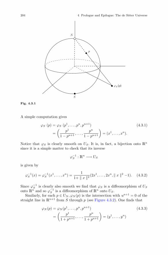
204 4 Prologue and Epilogue: The de Sitter Universe
N
p
S
'S (p)
Fig. 4.3.1
A simple computation gives
ϕS (p) = ϕS (p1, . . . , pn, pn+1) (4.3.1)
=(
p1
1 − pn+1, . . . ,
pn
1 − pn+1
)= (x1, . . . , xn).
Notice that ϕS is clearly smooth on US . It is, in fact, a bijection onto Rn
since it is a simple matter to check that its inverse
ϕ−1S : Rn −→ US
is given by
ϕ−1S (x) = ϕ−1
S (x1, . . . , xn) =1
1+ ‖ x ‖2(2x1, . . . , 2xn, ‖ x ‖2 −1). (4.3.2)
Since ϕ−1S is clearly also smooth we find that ϕS is a diffeomorphism of US
onto Rn and so ϕ−1S is a diffeomorphism of Rn onto US.
Similarly, for each p ∈ UN , ϕN (p) is the intersection with un+1 = 0 of thestraight line in Rn+1 from S through p (see Figure 4.3.2). One finds that
ϕN (p) = ϕN (p1, . . . , pn, pn+1) (4.3.3)
=(
p1
1 + pn+1, . . . ,
pn
1 + pn+1
)= (y1, . . . , yn)
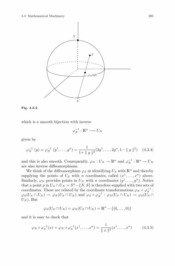
4.3 Mathematical Machinery 205
N
p
S
'N (p)
Fig. 4.3.2
which is a smooth bijection with inverse
ϕ−1N : Rn −→ UN
given by
ϕ−1N (y) = ϕ−1
N (y1, . . . , yn) =1
1+ ‖ y ‖2(2y1, . . . , 2yn, 1− ‖ y ‖2) (4.3.4)
and this is also smooth. Consequently, ϕN : UN → Rn and ϕ−1N : Rn → UN
are also inverse diffeomorphisms.We think of the diffeomorphism ϕS as identifying US with Rn and thereby
supplying the points of US with n coordinates, called (x1, . . . , xn) above.Similarly, ϕN provides points in UN with n coordinates (y1, . . . , yn). Noticethat a point p in US ∩ UN = Sn−{N, S} is therefore supplied with two sets ofcoordinates. These are related by the coordinate transformations ϕN ◦ ϕ−1
S :ϕS(US ∩ UN ) → ϕN (US ∩ UN ) and ϕS ◦ ϕ−1
N : ϕN (US ∩ UN) → ϕS(US ∩UN ). But
ϕS(US ∩ UN ) = ϕN (US ∩ UN ) = Rn − {(0, . . . , 0)}
and it is easy to check that
ϕN ◦ ϕ−1S (x) = ϕN ◦ ϕ−1
S (x1, . . . , xn) =1
‖ x ‖2(x1, . . . , xn) (4.3.5)

206 4 Prologue and Epilogue: The de Sitter Universe
and
ϕS ◦ ϕ−1N (y) = ϕS ◦ ϕ−1
N (y1, . . . , yn) =1
‖ y ‖2(y1, . . . , yn). (4.3.6)
The essential content of all this is that Sn is “locally diffeomorphic to Rn”in the sense that each point of Sn is contained in an open subset of Sn thatis diffeomorphic to Rn. This is the prototype for our next definition.
Let n and m be positive integers with n ≤ m. A subset M of Rm is calledan n-dimensional smooth manifold (or smooth n-manifold) if, for each p ∈ M ,there is an open set U in M containing p and a diffeomorphism ϕ : U → ϕ(U)of U onto an open subset ϕ(U) of Rn. Thus, Sn is an n-dimensional smoothmanifold in Rn+1.
Remark: There is a more general definition of “smooth manifold” that doesnot require M to be a subset of a Euclidean space (see Chapter 5 of [N3]),but this will suffice for our purposes.
Exercise 4.3.1 Show that every open ball in Rn is diffeomorphic to Rn andconclude that every point in a smooth n-manifold M is contained in an opensubset of M that is diffeomorphic to all of Rn.
The pair (U, ϕ) is called a chart on M . A smooth n-manifold is just a subsetM of some Euclidean space for which there exists a family {(Uα, ϕα) : α ∈ A}of charts
ϕα : Uα −→ ϕα(Uα) ⊆ Rn
with⋃
α∈A Uα = M . Each ϕα supplies the points of Uα with n coordinates,namely, those of its image in ϕα(Uα). If Uα ∩Uβ �= ∅, then a point p ∈ Uα ∩Uβ
is supplied with two sets of coordinates, say,
ϕα (p) = (x1, . . . , xn)
andϕβ (p) = (y1, . . . , yn).
These are related by the transformation equations
ϕα ◦ ϕ−1β : ϕβ(Uα ∩ Uβ) −→ ϕα(Uα ∩ Uβ)
(x1, . . . , xn) =(ϕα ◦ ϕ−1
β
)(y1, . . . , yn)
and
ϕβ ◦ ϕ−1α : ϕα(Uα ∩ Uβ) −→ ϕβ(Uα ∩ Uβ)
(y1, . . . , yn) =(ϕβ ◦ ϕ−1
α
)(x1, . . . , xn).
Rn is itself a smooth n-manifold with a global chart (Rn, idRn). The corre-sponding coordinates are just the standard coordinates u1, . . . , un. The same

4.3 Mathematical Machinery 207
is true of any open subset of Rn. To produce more interesting examples wewill need to develop a technique for manufacturing charts. One particularlysimple case is contained in the following exercise.
Exercise 4.3.2 Let V be an open set in Rn and g : V → R a smoothreal-valued function on V . Show that the graph {(x, g(x)) : x ∈ V } of g inRn+1 = Rn ×R is a smooth n-manifold with a global chart.
The sphere Sn is not the graph of a function of n variables, but it canbe covered by open sets each of which is the graph of a function, e.g., thehemispheres with ui > 0 and ui < 0 for i = 1, . . . , n + 1. These functions“parametrize” the hemispheres of Sn and the projections back onto the do-mains provide charts. There are, however, many other ways of parametrizingregions on the sphere. For example, the map
χ : [0, π] × [0, 2π] −→ R3
defined byχ(φ, θ) = (sin φ cos θ, sinφ sin θ, cosφ) (4.3.7)
maps into (in fact, onto) the 2-sphere S2 in R3 and parametrizes S2 bystandard spherical coordinates. The geometrical interpretation of φ and θ is
N
f
q
( sin f cos q, sin f sin q, cos f )
S
Fig. 4.3.3
the usual one from calculus (see Figure 4.3.3). Notice that χ is one-to-one on(0, π) × (0, 2π) and covers all of S2 except the north and south poles andthe longitudinal curve at θ = 0 (or θ = 2π) joining them. On this open setin S2, χ has an inverse and this has a chance of being a chart. In this caseone can actually calculate this inverse explicitly and show that it is, indeed,smooth and therefore a chart. To obtain a chart covering the longitudinal

208 4 Prologue and Epilogue: The de Sitter Universe
curve joining the north and south poles (but not N and S themselves) onecan use the same map χ, but on the open set (0, π) × (−π, π). To cover Nand S themselves one simply defines an analogous map, but measuring theangle φ from a different axis. It is customary to be a bit sloppy and refer toall of these collectively as “spherical coordinates” on S2.
We would like to apply this same idea in much more generality. Givena subset M of Rm we will find parametrizations of regions in M and hopeto “invert” them to obtain charts. More often than not, however, such in-verses are difficult or impossible to compute explicitly. Fortunately, there is aremarkable result from real analysis that can often relieve one of the responsi-bility of doing this. We will now state this result in the form most convenientfor our purposes and refer to [Sp1] for details.
If U is an open set in Rn and F : U → Rm is a smooth map we will writeF = (F 1, . . . , Fm) for the coordinate functions of F, DjF
i for the jth partialderivative of F i and, for each a ∈ U , the Jacobian of F at a will be written
F ′(a) = (Dj F i (a))1 ≤ i ≤ m1 ≤ j ≤ n
=
⎛⎜⎝D1F1(a) · · · DnF 1(a)...
...D1F
m(a) · · · DnFm(a)
⎞⎟⎠ .
The Inverse Function Theorem applies to the special case in which m = nand says that when the Jacobian F ′(a) is nonsingular, then F is a localdiffeomorphism near a. More precisely, we have
The Inverse Function Theorem: Let U be an open subset of Rn andF : U → Rn a smooth map. Suppose a ∈ U and F ′(a) is nonsingular (i.e.,detF ′(a) �= 0). Then there exist open sets V and W in Rn with a ∈ V ⊆ Uand F (a) ∈ W ⊆ Rn such that the restriction of F to V
F | V : V −→ W
is a diffeomorphism onto W, i.e., a smooth bijection with a smooth inverse
(F | V )−1 : W −→ V.
Moreover, ((F | V )−1
)′(F (a)) = (F | V )′ (a) .
Now let us suppose that we did not wish to go to the trouble of invertingthe spherical coordinate parametrization
χ : (0, π) × (0, 2π) −→ R3
χ(φ, θ) = (sin φ cos θ, sin φ sin θ, cosφ)
explicitly on its image in S2. We would like to use the Inverse FunctionTheorem to conclude nevertheless that it provides a chart at each point inthe image. Let’s write χ in more familiar notation as

4.3 Mathematical Machinery 209
x = sin φ cos θ
y = sin φ sin θ. (4.3.8)z = cosφ
Then the Jacobian of χ is given by
χ′(φ, θ) =
⎛⎜⎜⎜⎜⎜⎜⎜⎝
∂x
∂φ
∂x
∂θ
∂y
∂φ
∂y
∂θ
∂z
∂φ
∂z
∂θ
⎞⎟⎟⎟⎟⎟⎟⎟⎠=
⎛⎜⎜⎜⎝cosφ cos θ − sin φ sin θ
cosφ sin θ sin φ cos θ
− sin φ 0
⎞⎟⎟⎟⎠ .
We claim that, at each (φ, θ) ∈ (0, π)× (0, 2π), χ′(φ, θ) has maximal rank(namely, 2). To see this we compute the determinants of the various 2 × 2submatrices. ∣∣∣∣∣∣∣∣
∂x
∂φ
∂x
∂θ
∂y
∂φ
∂y
∂θ
∣∣∣∣∣∣∣∣ = cosφ sin φ
∣∣∣∣∣∣∣∣∂x
∂φ
∂x
∂θ
∂z
∂φ
∂z
∂θ
∣∣∣∣∣∣∣∣ = − sin2 φ sin θ
∣∣∣∣∣∣∣∣∂y
∂φ
∂y
∂θ
∂z
∂φ
∂z
∂θ
∣∣∣∣∣∣∣∣ = sin2 φ cos θ
For φ ∈ (0, π), sin φ �= 0 so, for any (φ, θ) ∈ (0, π) × (0, 2π), at least oneof these is nonzero. Let’s suppose we are at a point a = (φ0, θ0) at which∣∣∣∣∣∣∣∣
∂x
∂φ(a)
∂x
∂θ(a)
∂y
∂φ(a)
∂y
∂θ(a)
∣∣∣∣∣∣∣∣ �= 0
(the other cases are treated in the same way). Define an open set
U = (0, π) × (0, 2π) ×R
210 4 Prologue and Epilogue: The de Sitter Universe
in R3 and extend χ to a smooth map
χ : U −→ R3
by
χ(φ, θ, t) = (x(φ, θ), y(φ, θ), z(φ, θ) + t)= (sin φ cos θ, sin φ sin θ, cosφ + t).
The Jacobian of χ is ⎛⎜⎜⎜⎜⎜⎜⎜⎝
∂x
∂φ
∂x
∂θ0
∂y
∂φ
∂y
∂θ0
∂z
∂φ
∂z
∂θ1
⎞⎟⎟⎟⎟⎟⎟⎟⎠and this is nonsingular at (a, 0) = (φ0, θ0, 0) ∈ R3. Since χ(a, 0) = χ(a),the Inverse Function Theorem implies that there are open sets V and W inR3 with (a, 0) ∈ V ⊆ U and χ(a) ∈ W ⊆ R3 such that χ|V : V → W isa diffeomorphism. The restriction of this diffeomorphism to V ∩ ((0, π) ×(0, 2π)×{0}) is therefore a diffeomorphism of an open set in (0, π)× (0, 2π)(identified with (0, π) × (0, 2π)× {0}) containing a onto the intersection ofthe image of χ : (0, π) × (0, 2π) → R3 with W . But this intersection is anopen set in S2 containing χ(a) so the inverse of this last diffeomorphism is achart for S2 at χ(a).
The bottom line here is this. The smooth parametrization (4.3.8) hasmaximal rank at each point of (0, π) × (0, 2π) and from this alone theInverse Function Theorem implies that it can be smoothly inverted on anopen set about any point in (0, π) × (0, 2π), thus providing a chart in S2
near the image of that point. This is a very powerful technique that we willuse repeatedly, but one should not get carried away. Had we not known inadvance that χ : (0, π) × (0, 2π) → R3 is one-to-one, this would in no wayfollow from what we have done with the Inverse Function Theorem, whichguarantees invertibility only near a point where the Jacobian is nonsingular.Of course, since we do know that χ is one-to-one on (0, π)×(0, 2π) our argu-ments show that its inverse is smooth (a map on S2 is smooth, by definition,if it is smooth on some open set about each point).
In order to avoid repeating the same argument over and over again wewill now prove a general result that can be applied whenever we need tomanufacture a chart. Thus, let us suppose that M is a subset of some Rm, Uis an open set in Rn, where n ≤ m, and
χ : U −→ Rm

4.3 Mathematical Machinery 211
is a smooth map with χ(U) ⊆ M . Write x1, . . . , xn for the standardcoordinates on Rn and χ1, . . . , χn, . . . , χm for the coordinate functions of χ.Suppose a ∈ U is a point at which the Jacobian χ′(a) has rank n. Then somen×n submatrix of χ′(a) is nonsingular and, by renumbering the coordinatesif necessary, we may assume that⎛⎜⎝D1χ
1(a) · · · Dnχ1(a)...
...D1χ
n(a) · · · Dnχn(a)
⎞⎟⎠ =∂(χ1, . . . , χn)∂(x1, . . . , xn)
(a)
is nonsingular. If m = n, then the Inverse Function Theorem implies that χgives a chart at χ(a). Now assume n < m, define U = U ×Rm−n and let
χ : U −→ Rm
be defined by
χ(x, t) = χ(x1, . . . , xn, t1, . . . , tm−n)= (χ1(x), . . . , χn(x), χn+1(x) + t1, . . . , χm(x) + tm−n).
Then χ is smooth and its Jacobian at (a, 0) is⎛⎜⎜⎜⎝∂(χ1, . . . , χn)∂(x1, . . . , xn)
(a) O
∂(χn+1, . . . , χm)∂(x1, . . . , xn)
(a) I
⎞⎟⎟⎟⎠ ,
where O is the n × (m − n) zero matrix and I is the (m − n) × (m − n)identity matrix. This is nonsingular so the Inverse Function Theorem impliesthat there exist open sets V and W in Rm with (a, 0) ∈ V ⊆ U and χ(a, 0) =χ(a) ∈ W ⊆ Rm such that χ|V : V → W is a diffeomorphism. The restrictionof this diffeomorphism to V ∩ (U × {0}) is therefore a diffeomorphism of anopen set in U (identified with U × {0}) containing a onto the intersection ofthe image of χ : U → Rm with W . But this intersection is an open set in Mcontaining χ(a) so the inverse of this last diffeomorphism is a chart for Mat χ(a). We will refer to a smooth map χ : U → M ⊆ Rm, where U is openin Rn and χ′(a) is nonsingular for each a in U , as a coordinate patch for M .Thus, each point in the image χ(U) ⊆ M is contained in an open subset ofM on which χ−1 is a chart for M .
We will have occasion to use a great variety of charts (i.e., coordinatesystems) on the manifolds of interest to us so we will pause now to write outsome of these.
Example 4.3.1 We begin with a simple, but useful generalization of thespherical coordinate parametrization of S2. We define a map
χ : [0, π] × [0, π] × [0, 2π] −→ R4
212 4 Prologue and Epilogue: The de Sitter Universe
by
χ(φ1, φ2, θ)= (sin φ1 cos φ2, sin φ1 sin φ2 cos θ, sin φ1 sin φ2 sin θ, cos φ1).
Thus,
u1 = sin φ1 cosφ2
u2 = sin φ1 sin φ2 cos θ
u3 = sin φ1 sin φ2 sin θ (4.3.9)u4 = cosφ1.
A little trigonometry shows that (u1)2 +(u2)2 +(u3)2 +(u4)2 = 1 so χ mapsinto (in fact, onto) S3. The Jacobian is⎛⎜⎜⎜⎜⎝
cosφ1 cosφ2 − sinφ1 sin φ2 0
cosφ1 sin φ2 cos θ sinφ1 cosφ2 cos θ − sinφ1 sin φ2 sin θ
cosφ1 sinφ2 sin θ sin φ1 cosφ2 sin θ sin φ1 sin φ2 cos θ
− sinφ1 0 0
⎞⎟⎟⎟⎟⎠ .
Computing the determinants of all of the 3 × 3 submatrices we obtain
sin2 φ1 cosφ1 sinφ2
− sin3 φ1 sin2 φ2 sin θ
sin3 φ1 sin2 φ2 cos θ
− sin3 φ1 sin φ2 cosφ2.
Note that φ1 = 0 gives the point N = (0, 0, 0, 1) and φ1 = π gives S =(0, 0, 0,−1) and that all of the 3 × 3 determinants vanish at these points.These determinants also vanish when φ2 = 0 and φ2 = π. For (φ1,, φ2) ∈(0, π)× (0, π) one of the second or third determinants above is nonzero. Weconclude, in particular, that each point of (0, π)×(0, π)×(0, 2π) is containedin an open set on which χ is a diffeomorphism onto an open set in S3 and theinverse of this is a chart on S3 with coordinate functions (φ1,, φ2, θ). As forS2 one obtains charts at the remaining points of S3 by either replacing (0, 2π)with (−π, π) or interchanging the roles of some of the standard coordinateson R4 and these charts are collectively called spherical (or hyper-spherical)coordinates on S3. An obvious modification provides, for any ρ > 0, sphericalcoordinates
u1 = ρ sinφ1 cosφ2
u2 = ρ sinφ1 sinφ2 cos θ
u3 = ρ sinφ1 sinφ2 sin θ (4.3.10)u4 = ρ cosφ1
4.3 Mathematical Machinery 213
on the sphere(u1)2 + (u2)2 + (u3)2 + (u4)2 = ρ2
of radius ρ in R4.
Exercise 4.3.3 Show that, for ρ > 0 and for φ1, φ2 and θ exactly as in thecase of S3, (4.3.10) determines a chart at each point of R4 except the origin.
Next we turn to the manifold that will occupy most of our time. It is a 4-dimensional manifold in R5 and upon it we will build the de Sitter universe.Various different coordinate systems on it elucidate different aspects of itsgeometrical and physical structure so we will spend some time introducing anumber of them.
We consider the subset D of R5 given in terms of standard coordinatesu1, u2, u3, u4, u5 by
(u1)2 + (u2)2 + (u3)2 + (u4)2 − (u5)2 = 1.
Notice that the intersection of D with u5 = 0 is just S3 and, more generally,setting u5 equal to some constant value u5
0 gives a slice of D that is just a
3-sphere of radius√
1 + (u50)
2.
Exercise 4.3.4 Show that, in fact, D is diffeomorphic to S3 × R. Hint:Consider the map F : D → S3 ×R given by
F (u1, u2, u3, u4, u5) =((
1 + (u5)2)− 1
2 u1,(1 + (u5)2
)− 12 u2,(
1 + (u5)2)− 1
2 u3,(1 + (u5)2
)− 12 u4, u5
).
By virtue of the analogy between D and x2 + y2 − z2 = 1 in R3 we picture Das a “hyperboloid” in R5 whose cross-sections at constant u5 are 3-spheresrather than circles (see Figure 4.3.4).
Example 4.3.2 Our first parametrization of D is the most natural one inlight of this picture. We view D as a family of 3-spheres, one for each −∞ <u5 < ∞, with radii evolving hyperbolically and each such sphere parametrizedas in (4.3.10). Specifically, we define
u1 = cosh tG sinφ1 cosφ2
u2 = cosh tG sinφ1 sinφ2 cos θ
u3 = cosh tG sinφ1 sinφ2 sin θ (4.3.11)
u4 = cosh tG cosφ1
u5 = sinh tG

214 4 Prologue and Epilogue: The de Sitter Universe
u5
S3
Fig. 4.3.4
for 0 ≤ φ1 ≤ π, 0 ≤ φ2 ≤ π, 0 ≤ θ ≤ 2π, and −∞ < tG < ∞. Then(u1)2 + (u2)2 + (u3)2 + (u4)2 − (u5)2 = 1 and the image of the map is allof D. For any fixed t0G, the slice at u5 = sinh t0G is the spherical coordinateparametrization of the 3-sphere of radius cosh t0G.
Exercise 4.3.5 Write out the Jacobian of the map (4.3.11) and show thatit has rank 4 on
0 < φ1 < π, 0 < φ2 < π, 0 < θ < 2π, −∞ < tG < ∞
and0 < φ1 < π, 0 < φ2 < π, −π < θ < π, −∞ < tG < ∞
and so provides a chart at the image of each such point. Note that chartsat points with φ1 = 0, π and φ2 = 0, π can be obtained by interchangingstandard coordinates on R5.
We conclude that each point of D is contained in an open set on which(φ1, φ2, θ, tG) are local coordinates and for this reason they are often calledglobal coordinates for D, although the charts themselves are not globallydefined on D. The motivation behind the remaining parametrizations of Dthat we intend to introduce now may appear rather obscure, but will becomeclear after we have introduced some geometry into our picture.

4.3 Mathematical Machinery 215
Example 4.3.3 The parametrization of D we introduce here differs fromthe global coordinates (φ1, φ2, θ, tG) only in that we will replace tG by anew fourth coordinate tC that we would like to be related to tG by
dtG
dtC= cosh tG
tC = 0 ⇐⇒ tG = 0
(the reason we would like this will emerge shortly). Separating variables,integrating the equation and using the initial condition gives
tC = 2 arctan(etG) − π
2(4.3.12)
so that−π
2< tC <
π
2.
Exercise 4.3.6 Show that
cosh tG =1
cos tC
for −π2
< tC < π2.
It follows that the mapping (φ1, φ2, θ, tC) → (φ1, φ2, θ, tG) is smooth withnonsingular Jacobian for −π
2 < tC < π2 and is therefore a local diffeomor-
phism. Composing this with the global coordinate parametrization of D wefind that each point of D is contained in an open set on which (φ1, φ2, θ, tC)are coordinates. For reasons that we will describe in Section 4.5 these arecalled conformal coordinates.
Example 4.3.4 Next we introduce what are called planar coordinates.These are denoted (tP , x1, x2, x3) and cover only half of D. They arisefrom the mapping
χ : R4 −→ R5
defined by
u1 = x1 etP
u2 = x2 etP
u3 = x3 etP (4.3.13)
u4 = cosh tP − 12
((x1)2
+(x2)2
+(x3)2)
etP
u5 = sinh tP + 12
((x1)2
+(x2)2
+(x3)2)
etP .
It is easy to check that (u1)2 + (u2)2 + (u3)2 + (u4)2 − (u5)2 = 1, but in thiscase
u4 + u5 = etP

216 4 Prologue and Epilogue: The de Sitter Universe
so only the portion u4 + u5 > 0 of D is covered by the image. For these,tP = ln(u4 + u5) and so
x1 =u1
u4 + u5
x2 =u2
u4 + u5(4.3.14)
x3 =u3
u4 + u5
tP = ln(u4 + u5).
We will denote by D+ this portion of D. The tP = t0P slices of D+ are theintersections with D+ of the hyperplanes u4 + u5 = et0P (see Figure 4.3.5).
u4 + u5 = etoP
u4 + u5 = 0
u5
Fig. 4.3.5
Exercise 4.3.7 Compute the Jacobian of (4.3.13) and show that it has rank4 at each point of R4.
Thus, each point of D+ is contained in an open subset of D+ on which(x1, x2, x3, tP ) are coordinates.
4.3 Mathematical Machinery 217
Example 4.3.5 Our final parametrization of D provides it with what arecalled hyperbolic coordinates (φ, θ, ψ, tH). We will leave the details to thereader.
Exercise 4.3.8 Define a smooth map of R4 into R5 by
u1 = cosφ sinh tH sinh ψ
u2 = sin φ cos θ sinh tH sinh ψ
u3 = sin φ sin θ sinh tH sinh ψ (4.3.15)u4 = cosh tH
u5 = sinh tH coshψ
(a) Verify that (u1)2 + (u2)2 + (u3)2 + (u4)2 − (u5)2 = 1.(b) Let t0H be a constant and consider the tH = t0H slice of D. Show that if
t0H = 0 this slice is a point and if t0H �= 0 the points on the slice haveu4 = cosh t0H and
(u1)2 + (u2)2 + (u3)2 − (u5)2 = − sinh2 t0H .
(c) Let t0H and ψ0 be two nonzero constants and consider the set of points inD with tH = t0H and ψ = ψ0. Show that u4 and u5 are constant and φand θ parametrize a 2-sphere in (u1, u2, u3)-space.
(d) Compute the Jacobian of (4.3.15) and show that it is nonsingular for0 < φ < π, 0 < θ < 2π, ψ �= 0, and tH �= 0.
With these examples in hand we now return to the general development.Each point on a smooth surface in R3 has associated with it a 2-dimensional“tangent plane” consisting of all the velocity vectors to all smooth curvesin the surface through that point. The analogous construction on a smoothn-manifold M in Rm proceeds as follows. We will write u1, . . . , um for thestandard coordinates in Rm and use x1, . . . , xn for standard coordinates inRn. If I ⊆ R is a (nondegenerate) interval, then a continuous map
α : I −→ M
α(t) = (u1(t), . . . , um(t))
is called a curve in M . α is said to be smooth if each ui(t), i = 1, . . . , m, isC∞ and if α’s velocity vector (or tangent vector)
α′(t) =(
du1
dt, . . . ,
dum
dt
)is nonzero for each t in I. Useful examples of smooth curves can be con-structed from a coordinate patch
χ : U −→ M ⊆ Rm
χ(x1, . . . , xn) = (u1(x1, . . . , xn), . . . , um(x1, . . . , xn)).
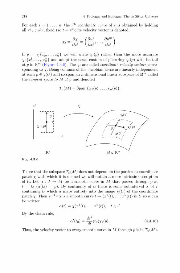
218 4 Prologue and Epilogue: The de Sitter Universe
For each i = 1, . . . , n, the ith coordinate curve of χ is obtained by holdingall xj , j �= i, fixed (so t = xi); its velocity vector is denoted
χi =∂χ
∂xi=(
∂u1
∂xi, . . . ,
∂um
∂xi
).
If p = χ(x1
0, . . . , xn0
)we will write χi(p) rather than the more accurate
χi
(x1
0, . . . , xn0
)and adopt the usual custom of picturing χi(p) with its tail
at p in Rm (Figure 4.3.6). The χi are called coordinate velocity vectors corre-sponding to χ. Being columns of the Jacobian these are linearly independentat each p ∈ χ(U) and so span an n-dimensional linear subspace of Rm calledthe tangent space to M at p and denoted
Tp(M) = Span {χ1(p), . . . , χn(p)}.
�−1( p)
�j( p)
�i( p)
�(U )
p
IRn
xi
�
U
xj
M ⊆ IRm
Fig. 4.3.6
To see that the subspace Tp(M) does not depend on the particular coordinatepatch χ with which it is defined we will obtain a more intrinsic descriptionof it. Let α : I → M be a smooth curve in M that passes through p att = t0 (α(t0) = p). By continuity of α there is some subinterval J of Icontaining t0 which α maps entirely into the image χ(U) of the coordinatepatch χ. Then χ−1 ◦α is a smooth curve t → (x1(t), . . . , xn(t)) in U so α canbe written
α(t) = χ(x1(t), . . . , xn(t)), t ∈ J.
By the chain rule,
α′(t0) =dx i
dt(t0)χi(p). (4.3.16)
Thus, the velocity vector to every smooth curve in M through p is in Tp(M).

4.3 Mathematical Machinery 219
Exercise 4.3.9 Show that, conversely, every nontrivial linear combina-tion of χ1(p), . . . , χn(p) is the velocity vector of some smooth curve in Mthrough p.
Thus, Tp(M) can be identified with the set of velocity vectors to smoothcurves in M through p (together with the zero vector which one can thinkof as the velocity vector to the, admittedly nonsmooth, constant curve inM through p). In particular, the coordinate velocity vectors for any othercoordinate patch
χ : U −→ M
with p ∈ χ(U) lie in Tp(M) and so span the same subspace of Rm.
Exercise 4.3.10 Let x1, . . . , xn and x1, . . . , xn denote the coordinates in Uand U , respectively, and χ : U → M and χ : U → M coordinate patcheswith χ(U) ∩ χ(U) �= ∅. Then on χ−1(χ(U) ∩ χ(U)) the map χ−1 ◦χ givesx1, . . . , xn as functions of x1, . . . , xn
xi = xi(x1, . . . , xn), i = 1, . . . , n,
andχ(x1, . . . , xn) = χ(x1(x1, . . . , xn), . . . , xn(x1, . . . , xn)).
Show that, at each point of χ−1(χ(U) ∩ χ(U )),
χi =∂xj
∂xiχj , i = 1, . . . , n.
Show, moreover, that if p ∈ χ(U) ∩ χ(U) and v ∈ Tp(M) with v = viχi(p)and v = vj χj(p), then
vj =∂xj
∂xi(χ−1(p))vi, j = 1, . . . , n.
The elements of Tp(M) are called tangent vectors to M at p.Since we have determined that the event world is “locally like M” at each
of its points we elect to model it by a smooth 4-manifold whose tangent spacesare all provided with the structure of Minkowski spacetime, i.e., a Lorentzinner product. A smooth assignment of an inner product to each tangentspace of a manifold is called a “metric” on M (not to be confused with theterm used in topology for a “distance function”, although there are someconnections). More precisely, a metric (or metric tensor) g on a manifold Mis an assignment to each tangent space Tp(M), p ∈ M , of an inner productgp = 〈 , 〉p such that the component functions gij defined by
gij (x1, . . . , xn) = gp(χi(p), χj(p)) = 〈χi(p), χj(p)〉p
are smooth on U for each coordinate patch χ : U → M . If each innerproduct gp has index zero, g is called a Riemannian metric on M ; if each

220 4 Prologue and Epilogue: The de Sitter Universe
gp has index 1, then g is a Lorentzian (or Lorentz ) metric. A spacetime isa smooth 4-manifold on which is defined a Lorentzian metric. In Euclideanspace Rn, for example, one can take the identity map χ = idRn as a globalchart so that χ1, . . . , χn are constant and equal to the standard basis vectorse1, . . . , en for Rn. Each Tp(Rn) can therefore be identified with Rn and onecan define a Riemannian metric g on Rn by simply taking gp = 〈 , 〉 foreach p ∈ Rn. Then gij (p) = δij , i, j = 1, . . . , n, for each p. On R4 one candefine a Lorentzian metric g by specifying that the inner product gp on eachTp(R4) = R4 satisfies gp (χi(p), χj(p)) = gp(ei, ej) = ηij , i, j = 1, 2, 3, 4. Theresulting spacetime is often denoted R3,1 although, morally at least, it is justMinkowski spacetime M.
Exercise 4.3.11 Suppose M is a manifold and g is a metric defined onM . Let χ : U → M and χ : U → M be coordinate patches for M withχ(U)∩ χ(U) �= ∅ and with coordinates x1, . . . , xn on U and x1, . . . , xn on U .Show that
gij =∂xk
∂xi
∂xl
∂xjgkl , i, j = 1, . . . , n.
and conclude that, if the gkl are smooth, then so are the gkl . Thus, at anypoint it is enough to check smoothness in a single coordinate patch.
The examples of interest to us here (but certainly not all interesting ex-amples) arise in a very simple way. If M is an n-manifold in Rm, then onecan endow Rm with various inner products and simply “restrict” these toeach Tp(M). We will illustrate the idea first for S2 ⊆ R3.
Consider a spherical coordinate parametrization
χ(φ, θ) = (sin φ cos θ, sin φ sin θ, cosφ)
of S2(x1 = φ, x2 = θ). The coordinate velocity vectors (columns of theJacobian) are
χ1 = χφ = (cosφ cos θ, cosφ sin θ, − sinφ)
andχ2 = χθ = (− sin φ sin θ, sin φ cos θ, 0).
At each point in the image of χ these are tangent vectors which we can regardas vectors in R3 and compute the R3-inner products
〈χ1, χ1〉 = cos2 φ cos2 θ + cos2 φ sin2 θ + sin2 φ = 1〈χ2, χ2〉 = sin2 φ sin2 θ + sin2 φ cos2 θ = sin2 φ
〈χ1, χ2〉 = 〈χ2, χ1〉 = 0.
Thus, if we define a (Riemannian) metric g on S2 by taking gp(v, w) = 〈v, w〉for each p ∈ S2 and all v, w ∈ Tp(S2) ⊆ R3 the components gij , i, j = 1, 2,are given by

4.3 Mathematical Machinery 221(g11 g12
g21 g22
)=(
1 00 sin2 φ
)(4.3.17)
and these are certainly smooth.
Exercise 4.3.12 Define a Riemannian metric on S3 by restricting the usualEuclidean inner product 〈 , 〉 on R4 to each Tp(S3), p ∈ S3. Show that themetric components gij , i, j = 1, 2, 3, relative to the spherical coordinatesx1 = φ1, x2 = φ2, x3 = θ given by (4.3.9) are⎛⎝g11 g12 g13
g21 g22 g23
g31 g32 g33
⎞⎠ =
⎛⎝1 0 00 sin2 φ1 00 0 sin2 φ1 sin2 φ2
⎞⎠ .
To obtain examples of Lorentz metrics in this way we will need to be-gin with an inner product of index one on some Rm to restrict to a man-ifold M ⊆ Rm. This can be done in any dimension, but we will restrictour attention to the one example we would like to understand, that is, thede Sitter spacetime. For this we begin with the 5-dimensional analogue ofMinkowski spacetime. Specifically, on R5 with standard coordinate functionsu1, . . . , u4, u5 we introduce an inner product denoted ( , ) and defined by
(p, q) = ((p1, . . . , p4, p5), (q1, . . . , q4, q5))= p1q1 + · · · + p4q4 − p5q5
= ηij piqj ,
where
ηij =
⎧⎪⎨⎪⎩1 , i = j = 1, 2, 3, 4
−1 , i = j = 50 , i �= j
(using η for this as well as the corresponding matrix for M should lead to noconfusion since the context will always indicate which is intended). We willdenote by M5 the real vector space R5 with this inner product. Notice thatthe manifold D in R5 is just the set of points p in M5 with
(p, p) = 1.
We now appropriate for M5 all of the basic terminology and notation in-troduced for Minkowski spacetime, e.g., v ∈ M5 is spacelike if (v, v) > 0,timelike if (v, v) < 0 and null if (v, v) = 0, the null cone CN (x0) at anyx0 ∈ M5 is the set CN(x0) = {x ∈ M5 : (x−x0, x−x0) = 0}, the time coneat x0 is CT (x0) = {x ∈ M5 : (x − x0, x − x0) < 0}, and so on. Indeed, all ofthe basic geometry of M is completely insensitive to the number of “spatialdimensions” and so generalizes immediately to M5. Use the following fewexercises as an opportunity to persuade yourself that this is true.
222 4 Prologue and Epilogue: The de Sitter Universe
Exercise 4.3.13 Prove that two nonzero null vectors v and w in M5 areorthogonal if and only if they are parallel.
Exercise 4.3.14 Let {e1, . . . , e4, e5} be any orthonormal basis for M5
((ei, ej) = ηij ). Show that if v = viei is timelike and w = wjej is eithertimelike or null and nonzero, then either
(a) v5w5 > 0, in which case (v, w) < 0, or(b) v5w5 < 0, in which case (v, w) > 0.
With this last exercise one can introduce time orientations (future-directedand past-directed) for timelike and nonzero null vectors in M5 in preciselythe same way as it was done in Minkowski spacetime (Section 1.3).
Exercise 4.3.15 Prove that the sum of any finite number of vectors in M5,all of which are timelike or null and all future-directed (resp., past-directed)is timelike and future-directed (resp., past-directed) except when all of thevectors are null and parallel, in which case the sum is null and future-directed(resp., past-directed).
The causality relations � and < are defined on M5 just as they are onM (x � y ⇐⇒ y − x is timelike and future-directed and x < y ⇐⇒ y − x isnull and future-directed) and all of their basic properties are proved in thesame way.
Exercise 4.3.16 Show that, for distinct points x and y in M5,
x < y if and only if
{x /� y andy� z =⇒ x � z
.
An orthogonal transformation of M5 is a linear transformation L :M5 →M5. satisfying (Lx ,Ly) = (x, y) for all x, y ∈ M5 and these have matri-ces Λ =
(Λi
j
)i,j=1,2,3,4,5
relative to orthonormal bases defined exactly as inM (Section 1.2) which satisfy ΛT ηΛ = η, where η = (ηij )i,j=1,2,3,4,5. Thosewhich satisfy, in addition, Λ5
5 ≥ 1 are called orthochronous and these pre-serve the time orientation of all timelike and nonzero null vectors and so pre-serve the causality relations (x � y ⇐⇒ Lx � Ly and x < y ⇐⇒ Lx < Ly).Just as in M, ΛT ηΛ = η implies det Λ = ±1 and we single out those withdetΛ = 1 to refer to as proper. The collection
L5 ={Λ =(Λi
j
)i,j=1,2,3,4,5
: ΛT ηΛ = η, Λ55 ≥ 1, detΛ = 1
}is the analogue in M5 of the proper, orthochronous Lorentz group L.
And so the story goes. Essentially everything purely geometrical that wehave said about M and L is equally true of M5 and L5. Indeed, evenZeeman’s Theorem 1.6.2 remains true for M5. More precisely, a bijectionF : M5 → M5 satisfying x < y if and only if F (x) < F (y) (or, equivalently,
4.3 Mathematical Machinery 223
x � y if and only if F (x) � F (y)) is called a causal automorphism and oneproves, essentially as in Section 1.6, that any such is the composition of anorthochronous orthogonal transformation of M5, a translation of M5 anda dilation of M5. We will not belabor this point any further here, but willsimply leave it to the skeptical reader to check that when we need a resultproved for M to be true in M5, it is.
Of course, something is lost in moving from M to M5 and that is thephysical interpretation (the event world is, to the best of our knowledge,4-dimensional, not 5-dimensional). To return to physics we must return toD ⊆ M5.
Our intention is to do for D ⊆ M5 what we did for S2 ⊆ R3 and S3 ⊆ R4,that is, restrict the inner product of the ambient space to each tangent spaceof the manifold, thereby defining a metric.
Remark: The fact that we actually get a metric in this way is not as obviousas it was in the positive definite case. The restriction of ( , ) to each Tp(D)is surely bilinear and symmetric, but is not obviously nondegenerate nor isit obviously of index one. That it is, in fact, nondegenerate and of index onewill follow from the calculations we are about to perform.
We will describe the metric components first in global coordinates (x1 = φ1,x2 = φ2, x3 = θ, x4 = tG). The coordinate velocity vectors are, fromExample 4.3.2,
χ1 = χφ1 = (cosh tG cosφ1 cosφ2, cosh tG cosφ1 sinφ2 cos θ,
cosh tG cosφ1 sinφ2 sin θ, − cosh tG sin φ1, 0)
χ2 = χφ2 = (− cosh tG sin φ1 sin φ2, cosh tG sin φ1 cosφ2 cos θ,
cosh tG sin φ1 cosφ2 sin θ, 0, 0)
χ3 = χθ = (0, − cosh tG sin φ1 sin φ2 sin θ,
cosh tG sin φ1 sinφ2 cos θ, 0, 0)
χ4 = χtG = (sinh tG sin φ1 cosφ2, sinh tG sinφ1 sinφ2 cos θ,
sinh tG sin φ1 sin φ2 sin θ, sinh tG cosφ1, cosh tG).
Thus, for example,
g11 = (χ1, χ1) = cosh2 tG cos2 φ1 cos2 φ2 + cosh2 tG cos2 φ1 sin2 φ2 cos2 θ
+ cosh2 tG cos2 φ1 sin2 φ2 sin2 θ + cosh2 tG sin2 φ1 − 0
= cosh2 tG [cos2 φ1 cos2 φ2 + cos2 φ1 sin2 φ2 + sin2 φ1]
= cosh2 tG
g44 = (χ4, χ4) = sinh2 tG sin2 φ1 cos2 φ2 + sinh2 tG sin2 φ1 sin2 φ2 cos2 θ
+ sinh2 tG sin2 φ1 sin2 φ2 sin2 θ + sinh2 tG cos2 φ1
− cosh2 tG
224 4 Prologue and Epilogue: The de Sitter Universe
= sinh2 tG[sin2 φ1 cos2 φ2 + sin2 φ1 sin2 φ2 cos2 θ
+ sin2 φ1 sin2 φ2 sin2 θ + cos2 φ1
]− cosh2 tG
= sinh2 tG − cosh2 tG
= −1
g23 = (χ2, χ3) = 0 − cosh2 tG sin2 φ1 sin φ2 cosφ2 sin θ cos θ
+ cosh2 tG sin2 φ1 sin φ2 cosφ2 sin θ cos θ
= 0
Exercise 4.3.17 Compute the rest and show that the only nonzerogij , i, j = 1, 2, 3, 4, are
g11 = cosh2 tG
g22 = cosh2 tG sin2 φ1
g33 = cosh2 tG sin2 φ1 sin2 φ2
g44 = −1
Notice that the restriction of the M5 inner product does, indeed, define aLorentz metric on D since, at each point p ∈ D, there is a basis e1, e2, e3, e4
for the tangent space Tp(D) satisfying g(ei, ej) = ηij , i, j = 1, 2, 3, 4. Indeed,one can take e4 = χ4(p) and let e1, e2, e3 be the normalized versions ofχ1, χ2, χ3, i.e.,
e1 =1
cosh tGχ1(p)
e2 =1
cosh tG sin φ1χ2(p)
e3 =1
cosh tG sin φ1 sin φ2χ3(p).
With this Lorentz metric, D is called the de Sitter spacetime and will bedenoted dS.
Before recording more examples we will introduce a more traditional andgenerally more convenient means of displaying the metric components. Wewill illustrate the idea first for the 2-sphere S2. To facilitate the notation wewill (temporarily) denote the standard spherical coordinates φ and θ on S2
by x1 and x2, respectively.
χ : (0, π) × (0, 2π) −→ S2
χ(x1, x2) = (sin(x1) cos(x2), sin(x1) sin(x2), cos(x1))
4.3 Mathematical Machinery 225
Let α : [a, b] → S2 be a smooth curve in S2 given by
α(t) = χ(x1(t), x2(t))= (sin(x1(t)) cos(x2(t)), sin(x1(t)) sin(x2(t)), cos(x1(t))).
For each t in [a, b], the Chain Rule gives
α′(t) =dx 1
dxχ1(x1(t), x2(t)) +
dx 2
dtχ2 (x1(t), x2(t))
=dx i
dtχi(x1(t), x2(t)).
The Riemannian metric g we have defined on S2 allows us to compute thesquared magnitude of α′(t) as follows.
g(α′(t), α′(t)) = g
(dx i
dtχi,
dx j
dtχj
)
=dx i
dtdx j
dtg(χi, χj)
= gijdx i
dtdx j
dt
The square root of g(α′(t), α′(t)) is the curve’s “speed” which, when inte-grated from a to t gives the arc length s = s(t). Consequently,(
dsdt
)2
= gijdx i
dtdx j
dt
which it is customary to write more succinctly in “differential form” as
ds2 = gij dx i dx j .
Reverting to φ and θ and substituting the values of gij that we have computed((4.3.17)) gives
ds2 = dφ2 + sin2 φdθ2. (4.3.18)
This is generally called the line element of S2. We regard it as a horizontaldisplay of the metric components g11 = 1, g22 = sin2 φ, g12 = g21 = 0 and aconvenient way to remember how to compute arc lengths.
Remark: The symbols in (4.3.18) can all be given precise meanings in thelanguage of differential forms, but we will have no need to do so.
The same notational device is employed for any Riemannian or Lorentzmetric. For example, writing x1 = x, x2 = y, x3 = z for the standardcoordinates on R3 one has
ds2 = dx 2 + dy2 + dz 2

226 4 Prologue and Epilogue: The de Sitter Universe
(g11 = g22 = g33 = 1 and gij = 0 for i, j = 1, 2, 3, i �= j), whereas, in sphericalcoordinates on R3,
ds2 = dρ2 + ρ2(dφ2 + sin2 φdθ2). (4.3.19)
For R3,1 it would be
ds2 = (dx 1)2 + (dx 2)2 + (dx 3)2 − (dx 4)2, (4.3.20)
while for S3 with spherical coordinates φ1, φ2, θ,
ds2 = dφ21 + sin2 φ1
(dφ2
2 + sin2 φ2dθ2). (4.3.21)
Finally, for de Sitter spacetime in global coordinates, Exercise 4.3.17 gives
ds2 = cosh2 tG(dφ2
1 + sin2 φ1
(dφ2
2 + sin2 φ2dθ2))
− dt2G. (4.3.22)
Exercise 4.3.18 Show that the line element for de Sitter spacetime, writtenin conformal coordinates (φ1, φ2, θ, tC) is
ds2 =1
cos2 tC
(dφ2
1 + sin2 φ1
(dφ2
2 + sin2 φ2dθ2)− dt2
C
).
Exercise 4.3.19 Show that the line element for de Sitter spacetime, writtenin planar coordinates (x1, x2, x3, tP ) is ds2 = e2tP ((dx 1)2 + (dx 2)2 +(dx 3)2) − dt2
P , or, using spherical coordinates for x1, x2, x3,
ds2 = e2tP (dρ2 + ρ2(dφ2 + sin2 φdθ2)) − dt2P .
Exercise 4.3.20 Show that the line element for de Sitter spacetime, writtenin hyperbolic coordinates (φ, θ, ψ, tH) is
ds2 = sinh2 tH(dψ2 + sinh2 ψ(dφ2 + sin2 φdθ2)) − dt2H .
One should notice, however, that in the case of dS (or any other Lorentzmanifold) the interpretation of the line element requires some care. Just asin Minkowski spacetime, a curve in dS might well have a velocity vector thatis null at each point so that gij
dx i
dtdx j
dtis zero everywhere and its “arc length”
is zero. If the velocity vector is timelike everywhere, then(dsdt
)2= gij
dx i
dtdxj
dt
would make dsdt pure imaginary. To exercise the proper care we mimic our
definitions for M.If M is a spacetime, then a smooth curve α : I → M is said to be spacelike,
timelike, or null if its tangent vector α′(t) satisfies gα(t)(α′(t), α′(t)) > 0,gα(t)(α′(t), α′(t)) < 0, or gα(t)(α′(t), α′(t)) = 0 for each t ∈ I. If I hasan endpoint t0 we require that these conditions be satisfied there as well inthe sense that any smooth extension of α to an open interval about t0 has atangent vector at t0 satisfying the required condition. Notice that in dS this

4.3 Mathematical Machinery 227
simply amounts to the requirement that each α′(t), regarded as a vector inM5 is spacelike, timelike or null in M5. We will say that a timelike or nullcurve in dS is future-directed (resp., past-directed) if each α′(t), regarded asa vector in M5, is future-directed (resp., past-directed).
Remark: The notion of a spacetime, as we have defined it, is very generaland there are examples in which it is not possible to define unambiguousnotions of future-directed and past-directed (see [HE], page 130). This isessentially a sort of “orientability” issue analogous to the fact that, for somesurfaces in R3 such as the Mobius strip, it is impossible to define a continuousnonzero normal vector field over the entire surface. We care only about Mand dS and so the issue will not arise for us.
A future-directed timelike curve in dS is called a timelike worldline and weascribe to such a curve the same physical interpretation we did in M (theworldline of some material particle). Just as in M one can define the propertime length L(α) of such a curve α : [a, b] → dS by
L(α) =∫ b
a
√−(α′(t), α′(t)) dt
and a proper time parameter τ = τ(t) along α by
τ = τ(t) =∫ t
a
√−(α′(u), α′(u)) du .
We will go even further and induce causality relations on dS from those onM5. Specifically, for distinct points x and y in dS we will define x � y if andonly if y − x is timelike and future-directed in M5 and x < y if and only ify − x is null and future-directed in M5.
Remark: Although we will have no need of the result, we point out that,with these definitions, Zeeman’s Theorem 1.6.2 remains true in dS in thefollowing sense. A bijection F : dS → dS that preserves < in both directionsalso preserves � in both directions and is, in fact, the restriction to dS ofsome orthochronous orthogonal transformation of M5 (see [Lest]).
Let us think for a moment about the sort of timelike curve in dS thatshould model the worldline of a material particle that is “free”, i.e., in freefall. As we saw in Section 4.2, at each point on such a worldline there is alocal inertial frame (freely falling elevator) from which it can be observedand that, relative to such a frame, the worldline will appear (approximately)“straight.” Curves in a manifold with (Riemannian or Lorentz) metric thatare “locally straight” are called geodesics. There are various approaches to theformulation of a precise definition, but we will follow a path that is adaptedto the simplicity of the examples we wish to consider. The motivation for ourapproach is most easily understood in the context of smooth surfaces in R3
so we will first let the reader work through some of this.
228 4 Prologue and Epilogue: The de Sitter Universe
Exercise 4.3.21 Let M be a smooth surface (i.e., 2-manifold) in R3 withRiemannian metric g obtained by restricting the R3-inner product 〈 , 〉 to eachtangent space. Let χ : U → M ⊆ R3 be a coordinate patch for M and letα = α(t) be a smooth curve in M whose image is contained in χ(U). At eacht the tangent vector α′(t) is, by definition, in Tα(t)(M), but the accelerationα′′(t) in general will not lie in Tα(t)(M) since it will have both tangential andnormal components, i.e.,
α′′(t) = α′′tan(t) + α′′
nor(t),
where α′′tan(t) ∈ Tα(t)(M) and 〈α′′
nor(t), v〉 = 0 for every v ∈ Tα(t)(M).
(a) Write α(t) = χ(x1(t), x2(t)) and show that
α′′(t) =d2xi
dt2 χi(x1(t), x2(t)) +dx i
dtdx j
dtχij (x1(t), x2(t)),
where
χij =∂
∂xjχi =
(∂2u1
∂xj∂xi,
∂2u2
∂xj∂xi,
∂2u3
∂xj∂xi
).
(b) Show that the cross product χ1 × χ2 is nonzero at each point of χ(U)and so N = χ1 × χ2/‖χ1 × χ2‖ is a unit normal vector to each pointof χ(U). Note: This normal vector field generally exists only locally onχ(U). There are surfaces (such as the Mobius strip) on which it is notpossible to define a continuous, nonvanishing field of normal vectors.
(c) Resolve χij into tangential and normal components to obtain
χij = Γrijχr + Lij N,
where 〈χij , χk〉 = Γrij grk and Lij = 〈χij , N〉.
(d) Define Γr,ij = grlΓlij and show that
∂gij
∂xk= Γi,jk + Γj,ik . (4.3.23)
(e) Denote by (gij ) the inverse of the matrix (gij ) and show that
Γrij =
12grk
(∂gik
∂xj+
∂gjk
∂xi− ∂gij
∂xk
). (4.3.24)
Hint: Permute the indices i j k in (4.3.23) to obtain expressions for eachof the derivatives in (4.3.24) and combine them using the symmetriesΓi,jk = Γi,kj , i, j, k = 1, 2.

4.3 Mathematical Machinery 229
(f) Conclude that
α′′tan(t) =
(d2xr
dt2+ Γr
ij (x1(t), x2(t))
d xi
dtd xj
dt
)χr(x1(t), x2(t))
andα′′
nor(t) = Lij (x1(t), x2(t)) N(x1(t), x2(t)).
If, in Exercise 4.3.21, t = s is the arc length parameter for α, then α′′(s) isthe curvature vector of α. One regards α′′
nor as that part of α’s curvature thatit must possess simply by virtue of the fact that it is constrained to remainin M , whereas α′′
tan is the part α contributes on its own by “curving in M .”Curves with α′′
tan = 0 are thought to “curve only as much as they must toremain in M” and so are the closest thing in M to a straight line (we willsee shortly that in S2 these are just constant speed parametrizations of greatcircles, i.e., intersections of S2 with planes through the origin in R3).
There is only one obstacle to carrying out the entire calculation inExercise 4.3.21 for any χ(U) on an n-manifold M in Rm and that is ex-istence of the unit normal field N . In Rm, m > 3, there is no naturalconcept of a cross product and, in any case, the tangent space Tp(M) isnot spanned by just two vectors. For the simple examples of interest to us,however, the obstacle is easily overcome. At each point p on the n-sphereSn ⊆ Rn+1, for instance, the vector p in Rn+1 is itself a unit normal vectorto Tp(Sn). Indeed, if α is any smooth curve in Sn through p at t = t0, thenα(t) = (u1(t), . . . , un+1(t)) implies
(u1(t))2 + · · · + (un+1(t))2 = 1
so
2u1(t)du1
dt+ · · · + 2un+1(t)
dun+1
dt= 0
which, at t = t0, gives〈p, α′(t0)〉 = 0.
Similarly, if p ∈ dS ⊆ M5 and α(t) = (u1(t), · · · , u5(t)) is a smooth curve indS with α(t0) = p, then
(u1(t))2 + · · · + (u4(t))2 − (u5(t))2 = 1
gives(p, α′(t0)) = 0
so p is a unit normal vector to Tp(dS ) (“unit” and “normal” now refer to theLorentz metric of dS, of course).
230 4 Prologue and Epilogue: The de Sitter Universe
In either of these cases the calculations in Exercise 4.3.21 (with N replacedby N(p) = p) can be repeated verbatim to resolve the acceleration α′′(t) ofa smooth curve into tangential and normal components with
α′′tan(t) =
(d2xr
d t2+ Γr
ij
d xi
dtd xj
dt
)χr (4.3.25)
in any coordinate patch, where
Γrij =
12grk
(∂gik
∂xj+
∂gjk
∂xi− ∂gij
∂xk
)(4.3.26)
(these are called the Christoffel symbols of the metric in the given coordinatesystem).
Those curves for which α′′tan(t) = 0 for each t are called geodesics and they
satisfyd2xr
dt2 + Γrij
d xi
dtd xj
dt= 0 (4.3.27)
in any coordinate patch.
Remark: Geodesics can be introduced in many ways and in much moregeneral contexts, but the end result is always the system (4.3.27) of ordinarydifferential equations. Notice that equations (4.3.27) are trivially satisfied byany constant curve α(t) = p ∈ M . Even though such constant curves are notsmooth in our sense we would like them to “count” and so we will refer tothem as degenerate geodesics.
To get some sense of the complexity of the equations (4.3.27) we shouldwrite them out in the case of most interest to us. Thus, we consider de Sitterspacetime dS in global coordinates x1 = φ1, x2 = φ2, x3 = θ, x4 = tG. FromExercise 4.3.17,
(gij ) = diag(cosh2 tG, cosh2 tG sin2 φ1, cosh2 tG sin2 φ1 sin2 φ2, −1)
so (gij ) is the diagonal matrix whose entries are the reciprocals of these.Because both of these are diagonal and independent of x3 = θ, the Christoffelsymbols (4.3.26) simplify a bit to
Γrij =
12grr
(∂gir
∂xj+
∂gjr
∂xi− ∂gij
∂xr
),
where there is no sum over r, all x3-derivatives vanish and all gkl with k �= lare zero. We compute a few of these.
Γ411 =
12g44
(0 + 0 − ∂g11
∂x4
)=
12(−1)(−2 cosh tG sinh tG)
= cosh tG sinh tG

4.3 Mathematical Machinery 231
Γ122 =
12g11
(0 + 0 − ∂g22
∂x1
)=
12
(1
cosh2 tG
)(cosh2 tG(−2 sinφ1 cosφ1))
= − sinφ1 cosφ1
Γ343 =
12g33
(0 +
∂g33
∂x4− 0)
=12
(1
cosh2 tG sin2 φ1 sin2 φ2
)·(
2 cosh tG sinh tG sin2 φ1 sin2 φ2
)=
sinh tGcosh tG
Γ221 =
12g22
(∂g22
∂x1+ 0 − 0
)=
12
(1
cosh2 tG sin2 φ1
)·
cosh2 tG(2 sinφ1 cosφ1)
=cosφ1
sinφ1.
Exercise 4.3.22 Show that the only nonvanishing Christoffel symbols fordS in global coordinates are as follows.
Γ411 = cosh tG sinh tG
Γ422 = cosh tG sinh tG sin2 φ1
Γ433 = cosh tG sinh tG sin2 φ1 sin2 φ2
Γi4i = Γi
i4 =sinh tGcosh tG
, i = 1, 2, 3
Γ122 = − sinφ1 cosφ1
Γ133 = − sinφ1 cosφ1 sin2 φ2
Γ233 = − sinφ2 cosφ2
Γ221 = Γ2
12 =cosφ1
sinφ1= Γ3
31 = Γ313
Γ332 =
cosφ2
sinφ2= Γ3
23.
With these one can write out the geodesic equations (4.3.27) for r = 1, 2, 3, 4.For example, if r = 1,
d2x1
dt2+ Γ1
ij
dxi
dtdxj
dt= 0
becomes
d2x1
dt2+ Γ1
22
(dx2
dt
)2
+ Γ133
(dx3
dt
)2
+ 2Γ141
dx4
dtdx1
dt= 0,
232 4 Prologue and Epilogue: The de Sitter Universe
or
d2φ1
dt2− sin φ1 cosφ1
(dφ2
dt
)2
− sin φ1 cosφ1 sin2 φ2
(dθ
dt
)2
+ 2sinh tGcosh tG
dtGdt
dφ1
dt= 0.
Exercise 4.3.23 Write out the r = 2, 3, and 4 equations to obtain a systemof four coupled second order ordinary differential equations for the geodesicsof dS.
The problem of explicitly solving the geodesic equations can be formidable.However, a few basic facts about systems of ordinary differential equations(and some inspired guesswork) will relieve us of this burden. For instance,(4.3.27) is nothing more that a system of second order ordinary differentialequations for the functions xi(t) so that standard existence and uniquenesstheorems for such systems imply that, for any given initial position α(t0) andinitial velocity α′(t0) there is a unique solution α(t) defined on some intervalabout t0 satisfying these initial conditions. More precisely, one obtains the
Existence and Uniqueness Theorem: Let M be a manifold with(Riemannian or Lorentzian) metric g and fix some t0 ∈ R. Then for anyp ∈ M and any v ∈ Tp(M) there exists a unique geodesic αv : Iv → Msuch that
1. αv(t0) = p, α′v(t0) = v, and
2. the interval Iv is maximal in the sense that if α : I → M is any geodesicsatisfying α(t0) = p and α′(t0) = v, then I ⊆ Iv and α = αv | I.
We will find the uniqueness asserted in this result particularly useful sinceit assures us that if we have somehow managed to conjure up geodesics inevery direction v at p, then we will, in fact, have all the geodesics through p.We will apply this procedure to a few examples shortly (e.g., by “guessing”that the geodesics of S2 should be great circles). First, however, we mustcome to understand that a geodesic is more than its image in M , which mustbe parametrized in a very particular way if it is to satisfy (4.3.27). First weshow that a given geodesic can be reparametrized in only a rather trivial wayif it is to remain a geodesic.
Lemma 4.3.1 Let M be a manifold with (Riemannian or Lorentzian) metricg and let α : I → M be a nondegenerate geodesic. Suppose J ⊆ R is aninterval and h : J → I, t = h(s), is a smooth function with h′(s) > 0 foreach s ∈ J . Then the reparametrization
β = α ◦ h : J −→ M
of α is a geodesic if and only if h(s) = as + b for some constants a and b.

4.3 Mathematical Machinery 233
Proof: The Chain Rule gives
β′(s) = α′(h(s))h′(s)
andβ′′(s) = α′′(h(s))(h′(s))2 + α′(h(s))h′′(s)
soβ′′
tan(s) = α′(h(s))h′′(s)
(α is a geodesic). Thus, β is a geodesic if and only if α′(h(s))h′′(s) = 0. Sinceα is a nondegenerate geodesic, α′ is never zero (otherwise uniqueness wouldimply that α is the constant curve). Thus, h′′(s) = 0 for every s in J soh(s) = as + b for some constants a and b. �
We can say much more about the parametrizations of a geodesic, however.We will now prove that geodesics are always constant speed curves.
Theorem 4.3.2 Let M be a manifold with (Riemannian or Lorentzian) met-ric g. Suppose α : I → M is a geodesic. Then g(α′(t), α′(t)) is constant on I.
Proof: We will show that ddt
g(α′(t), α′(t)) = 0 at each t in I. It will clearlysuffice to focus our attention on some subinterval of I that maps into χ(U) forsome coordinate patch χ : U → M ⊆ Rm. Writing α(t) = χ(x1(t), . . . , xn(t))we have
d
dt(g(α′(t), α′(t))) =
d
dt
(gij (x1(t), . . . , xn(t))
d xi
dtd xj
dt
).
To simplify the notation we will drop the arguments x1(t), . . . , xn(t) andcompute
d
dt
(gij
dxi
dtdxj
dt
)= gij
dxi
dtd2xj
dt2 + gijdxj
dtd2xi
dt2 +dg ij
dtdxi
dtdxj
dtd
dt
(gij
dxi
dtdxj
dt
)= 2gij
dxi
dtd2xj
dt2+
∂gij
∂xk
dxk
dtdxi
dtdxj
dt(4.3.28)
Now, d2xj
dt2= −Γj
abdxa
dtdxb
dtsince α is a geodesic so
2 gijd xi
dtd2 xj
dt2 = −2 gijΓjab
d xi
dtd xa
dtd xb
dt.
Moreover,
gijΓjab =
12gij gjk
(∂gak
∂xb+
∂gbk
∂xa− ∂gab
∂xk
)=
12δki
(∂gak
∂xb+
∂gbk
∂xa− ∂gab
∂xk
)=
12
(∂gai
∂xb+
∂gbi
∂xa− ∂gab
∂xi
)
234 4 Prologue and Epilogue: The de Sitter Universe
so
2 gijd xi
dtd2 xj
dt2 = −(
∂gai
∂xb+
∂gbi
∂xa− ∂gab
∂xi
)d xi
dtd xa
dtd xb
dt
= −∂gai
∂xb
d xb
dt
(d xi
dtd xa
dt
)−(
∂gib
∂xa− ∂gab
∂xi
)d xb
dt
(d xi
dtd xa
dt
).
Notice that the second term is skew-symmetric in a and i so the sum vanishes.Consequently,
2 gijdx i
dtd2xj
dt2 = −∂ gai
∂ xb
dx b
dt
(dx i
dtdxa
dt
)
= −∂ gij
∂ xk
dxk
dtdx i
dtdx j
dt
so (4.3.28) gives ddt
(gij
dx i
dtdxj
dt
)= 0 as required. �
Remark: It follows, in particular, from Theorem 4.3.2 that a geodesic ina spacetime manifold has the same causal character (spacelike, timelike, ornull) at each point. This is, of course, not true of an arbitrary smooth curve.
Example 4.3.6 No inspired guesswork is required to compute the geodesicsof Rn, or R3,1, or any manifold with a global chart in which the metriccomponents gij are constant. Here the Christoffel symbols Γr
ij are all zeroso the geodesic equations reduce to d2xr
dt2= 0 and the solutions are linear
functions of the coordinates.
Example 4.3.7 We consider the 2-sphere S2 with the Riemannian metric gobtained by restricting the Euclidean inner product 〈 , 〉 to each Tp(S2). Thus,
Tp(S2) = {v ∈ R3 : 〈p, v〉 = 0}.
We determine all of the geodesics of S2 through a fixed, but arbitrary point p.Of course, the degenerate geodesic is α0 : R → S2, defined by α0(t) = p foreach t ∈ R. Now fix some nonzero v ∈ Tp(S2). Then e = v/〈v, v〉 1
2 is a unitvector in R3 orthogonal to the unit vector p. Thus,
Span{e, p} = {ae + bp : a, b ∈ R}
is a 2-dimensional plane through the origin in R3. Its intersection with S2 isthe great circle on S2 consisting of all ae + bp with 〈ae + bp, ae + bp〉 = 1,i.e., a2 + b2 = 1. If we parametrize this circle by
αv(t) = (sin kt)e + (cos kt)p,−∞ < t < ∞,

4.3 Mathematical Machinery 235
where k = 〈v, v〉 12 , then
αv(0) = p
α′v(0) = ke = v.
Fig. 4.3.7
Moreover, g (α′v(t), α′
v(t)) = k2 = 〈v, v〉 is constant and α′′v (t) = −k2αv(t) =
−〈v, v〉αv(t) is everywhere normal to S2. Thus, αv(t) is the unique geodesicof S2 through p in the direction v. Since p and v were arbitrary we have foundall of the geodesics of S2.
Remark: Two of the fundamental undefined terms of classical planeEuclidean geometry are “point” and “straight line.” Identifying these un-defined terms with “point on S2” and “geodesic of S2,” respectively, oneobtains a system in which all of the axioms of plane Euclidean geometryare satisfied except the so-called Parallel Postulate (any two “straight lines”in S2 intersect; see Figure 4.3.7). This is Riemann’s spherical model ofnon-Euclidean geometry.
Exercise 4.3.24 Show in the same way that the nondegenerate geodesicsof the 3-sphere S3 are the constant speed parametrizations of its great circles(intersections with S3 of 2-dimensional planes through the origin in R4).
Example 4.3.8 Next we consider the de Sitter spacetime dS with theLorentz metric g obtained by restricting the 5-dimensional Minkowski in-ner product of M5 to each tangent space. According to the Remark follow-ing Theorem 4.3.2, we must now expect geodesics of three types (spacelike,timelike, and null), but the procedure for finding them is virtually identicalto what we have done for S2.
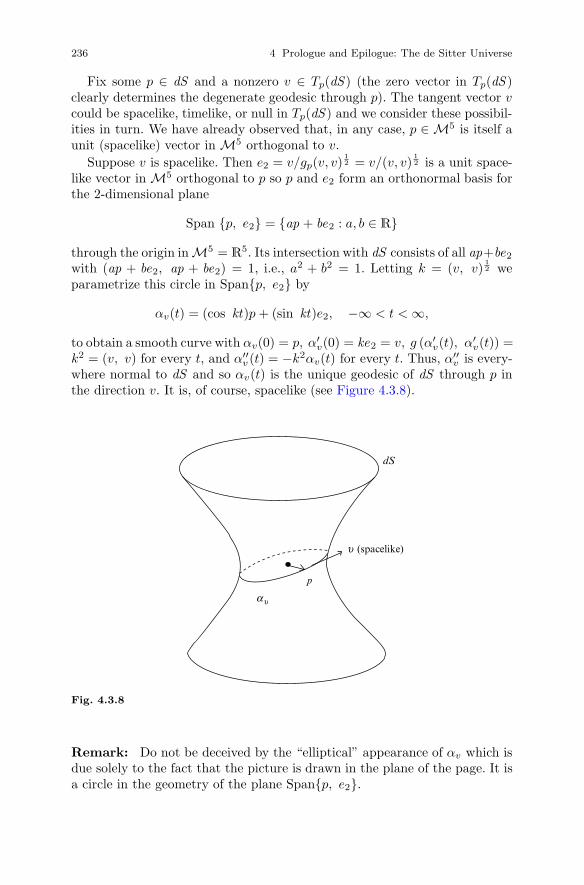
236 4 Prologue and Epilogue: The de Sitter Universe
Fix some p ∈ dS and a nonzero v ∈ Tp(dS ) (the zero vector in Tp(dS )clearly determines the degenerate geodesic through p). The tangent vector vcould be spacelike, timelike, or null in Tp(dS ) and we consider these possibil-ities in turn. We have already observed that, in any case, p ∈ M5 is itself aunit (spacelike) vector in M5 orthogonal to v.
Suppose v is spacelike. Then e2 = v/gp(v, v)12 = v/(v, v)
12 is a unit space-
like vector in M5 orthogonal to p so p and e2 form an orthonormal basis forthe 2-dimensional plane
Span {p, e2} = {ap + be2 : a, b ∈ R}
through the origin in M5 = R5. Its intersection with dS consists of all ap+be2
with (ap + be2, ap + be2) = 1, i.e., a2 + b2 = 1. Letting k = (v, v)12 we
parametrize this circle in Span{p, e2} by
αv(t) = (cos kt)p + (sin kt)e2, −∞ < t < ∞,
to obtain a smooth curve with αv(0) = p, α′v(0) = ke2 = v, g (α′
v(t), α′v(t)) =
k2 = (v, v) for every t, and α′′v (t) = −k2αv(t) for every t. Thus, α′′
v is every-where normal to dS and so αv(t) is the unique geodesic of dS through p inthe direction v. It is, of course, spacelike (see Figure 4.3.8).
au
p
dS
u (spacelike)
Fig. 4.3.8
Remark: Do not be deceived by the “elliptical” appearance of αv which isdue solely to the fact that the picture is drawn in the plane of the page. It isa circle in the geometry of the plane Span{p, e2}.
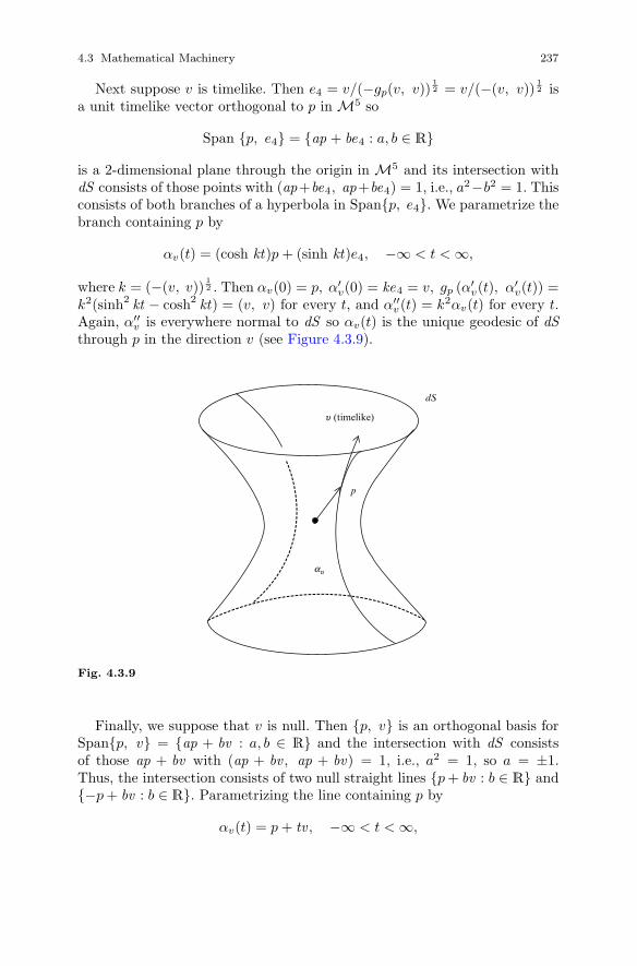
4.3 Mathematical Machinery 237
Next suppose v is timelike. Then e4 = v/(−gp(v, v))12 = v/(−(v, v))
12 is
a unit timelike vector orthogonal to p in M5 so
Span {p, e4} = {ap + be4 : a, b ∈ R}
is a 2-dimensional plane through the origin in M5 and its intersection withdS consists of those points with (ap+be4, ap+be4) = 1, i.e., a2−b2 = 1. Thisconsists of both branches of a hyperbola in Span{p, e4}. We parametrize thebranch containing p by
αv(t) = (cosh kt)p + (sinh kt)e4, −∞ < t < ∞,
where k = (−(v, v))12 . Then αv(0) = p, α′
v(0) = ke4 = v, gp (α′v(t), α′
v(t)) =k2(sinh2 kt − cosh2 kt) = (v, v) for every t, and α′′
v(t) = k2αv(t) for every t.Again, α′′
v is everywhere normal to dS so αv(t) is the unique geodesic of dSthrough p in the direction v (see Figure 4.3.9).
dS
u (timelike)
p
au
Fig. 4.3.9
Finally, we suppose that v is null. Then {p, v} is an orthogonal basis forSpan{p, v} = {ap + bv : a, b ∈ R} and the intersection with dS consistsof those ap + bv with (ap + bv , ap + bv) = 1, i.e., a2 = 1, so a = ±1.Thus, the intersection consists of two null straight lines {p + bv : b ∈ R} and{−p + bv : b ∈ R}. Parametrizing the line containing p by
αv(t) = p + tv , −∞ < t < ∞,
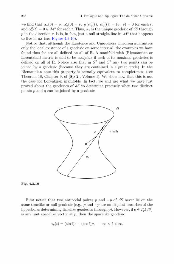
238 4 Prologue and Epilogue: The de Sitter Universe
we find that αv(0) = p, α′v(0) = v, g (α′
v(t), α′v(t)) = (v, v) = 0 for each t,
and α′′v (t) = 0 ∈ M5 for each t. Thus, αv is the unique geodesic of dS through
p in the direction v. It is, in fact, just a null straight line in M5 that happensto live in dS (see Figure 4.3.10).
Notice that, although the Existence and Uniqueness Theorem guaranteesonly the local existence of a geodesic on some interval, the examples we havefound thus far are all defined on all of R. A manifold with (Riemannian orLorentzian) metric is said to be complete if each of its maximal geodesics isdefined on all of R. Notice also that in S2 and S3 any two points can bejoined by a geodesic (because they are contained in a great circle). In theRiemannian case this property is actually equivalent to completeness (seeTheorem 18, Chapter 9, of [Sp 2], Volume I). We show now that this is notthe case for Lorentzian manifolds. In fact, we will use what we have justproved about the geodesics of dS to determine precisely when two distinctpoints p and q can be joined by a geodesic.
dS
u (null)p
au
Fig. 4.3.10
First notice that two antipodal points p and −p of dS never lie on thesame timelike or null geodesic (e.g., p and −p are on disjoint branches of thehyperbolas determining timelike geodesics through p). However, if e ∈ Tp(dS )is any unit spacelike vector at p, then the spacelike geodesic
αe(t) = (sin t)e + (cos t)p, −∞ < t < ∞,
4.3 Mathematical Machinery 239
satisfies αe(0) = p and αe(π) = −p. Thus, antipodal points can be joined by(many) spacelike geodesics.
Now suppose p and q are distinct, non-antipodal points in dS. Being indS, p and q are independent and so determine a unique 2-dimensional plane
Π = Span {p, q}
through the origin in M5. By what we have proved about the geodesics of dS,the only geodesic that could possibly join p and q is some parametrizationof (a part of) dS ∩ Π. Now, the restriction of the M5-inner product to Π,which we continue to denote ( , ), is clearly symmetric and bilinear. It maybe degenerate, or it may be nondegenerate and either of index zero or indexone. We consider these possibilities one at a time.
Suppose first that the restriction of ( , ) to Π is positive definite. Since pand q are unit spacelike vectors, dS ∩ Π is a circle and the parametrization
αq(t) = (cos t)p + (sin t)q, −∞ < t < ∞,
is a geodesic satisfying αq(0) = p and αq
(π2
)= q. In this case we claim that
we must have −1 < (p, q) < 1. To see this note that p ± q are nonzero sothat, since ( , ) is positive definite on Π,
0 < (p + q, p + q) = (p, p) + 2 (p, q) + (q, q) = 2 + 2 (p, q)
implies −1 < (p, q) and, similarly, 0 < (p − q, p − q) gives (p, q) < 1.Next suppose that the restriction of ( , ) to Π is nondegenerate of index one.
Then dS ∩Π consists of two branches of a hyperbola. We show that p and q lieon the same branch if and only if (p, q) > 1 (in which case p and q are joinedby a timelike geodesic) and on different branches if and only if (p, q) < −1 (inwhich case no geodesic joins p and q). To see this we choose an orthonormalbasis {e1, e2, e3, e4, e5} for M5 with (e5, e5) = −1 and Π = Span{e1, e5}.Then dS ∩ Π = {x1e1 +x5e5 : (x1)2−(x5)2 = 1} and the two branches of thehyperbola are given by x1 ≥ 1 and x1 ≤ −1. We parametrize these branchesby α1(t) = (cosh t)e1 + (sinh t)e5 and α2(t) = (− cosh t)e1 + (sinh t)e2. Now,if p and q are on the same branch, then for some i = 1, 2, p = αi(t0) andq = αi(t1) for some t0 �= t1 in R. Thus,
(p, q) = cosh t0 cosh t1 − sinh t0 sinh t1 = cosh (t0 − t1) > 1.
On the other hand, if p and q are on different branches, then p = αi(t0) andq = αj(t1), where i �= j, so
(p, q) = − cosh t0 cosh t1 − sinh t0 sinh t1 = − cosh (t0 + t1) < −1
as required.Finally, suppose that the restriction of ( , ) to Π is degenerate. Then dS ∩Π
consists of two parallel null straight lines
240 4 Prologue and Epilogue: The de Sitter Universe
α1(t) = p + tv
α2(t) = −p + tv,
where v ∈ Tp(dS ) satisfies (p, v) = 0 and (v, v) = 0. If p and q are on thesame line, then q = p + t0v for some t0 ∈ R so
(p, q) = (p, p + t0v) = (p, p) + t0(p, v) = 1.
and, if p and q are on different lines, then q = −p + t0v for some t0 ∈ R so
(p, q) = (p, −p + t0v) = (p, −p) + t0(p, v) = −1.
Now, since the conditions −1 < (p, q) < 1, (p, q) = 1, (p, q) > 1, and(p, q) ≤ −1 are mutually exclusive we can summarize all of this as follows.
Theorem 4.3.3 Let p and q be distinct points of dS and denote by ( , ) theMinkowski inner product on M5. Then
(a) If p and q are antipodal points of dS (q = −p), then p and q cannot bejoined by a timelike or null geodesic, but there are infinitely many spacelikegeodesics joining p and q.
If p and q are not antipodal points, then
(b) (p, q) > 1 ⇐⇒ p and q lie on a unique geodesic of dS which is timelike,(c) (p, q) = 1 ⇐⇒ p and q lie on a unique geodesic of dS which is null,(d) −1 < (p, q) < 1 ⇐⇒ p and q lie on a unique geodesic of dS which is
spacelike,(e) (p, q) ≤ −1 ⇐⇒ there is no geodesic of dS joining p and q.
It is worth pointing out that, for p, q ∈ dS , one has (p−q, p−q) = 2(1−(p, q))so that
(p, q) = 1 ⇐⇒ (p − q, p − q) = 0(p, q) > 1 ⇐⇒ (p − q, p − q) < 0
−1 < (p, q) < 1 ⇐⇒ 0 < (p − q, p − q) < 4(p, q) ≤ −1 ⇐⇒ (p − q, p − q) ≥ 4.
We will leave it to the reader to carry out a similar analysis of the importantexample of hyperbolic 3-space H3(r).
Exercise 4.3.25 M will denote (ordinary, 4-dimensional) Minkowski space-time and we will write x · y for the Minkowski inner product of x, y ∈ M.Standard admissible coordinates on M will be written x1, x2, x3, x4. Forany positive real number r we let H3(r) denote the subset of M defined by
H3(r) = {x ∈ M : x · x = −r2, x4 > 0},
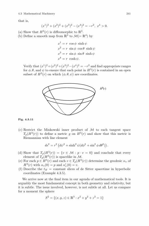
4.3 Mathematical Machinery 241
that is,(x1)2 + (x2)2 + (x3)2 − (x4)2 = −r2, x4 > 0.
(a) Show that H3(r) is diffeomorphic to R3.(b) Define a smooth map from R3 to M(= R4) by
x1 = r cosφ sinh ψ
x2 = r sin φ cos θ sinh ψ
x3 = r sin φ sin θ sinh ψ
x4 = r coshψ.
Verify that (x1)2+(x2)2+(x3)2−(x4)2 = −r2 and find appropriate rangesfor φ, θ, and ψ to ensure that each point in H3(r) is contained in an opensubset of H3(r) on which (φ, θ, ψ) are coordinates.
H3(r)
Fig. 4.3.11
(c) Restrict the Minkowski inner product of M to each tangent spaceTp(H3(r)) to define a metric g on H3(r) and show that this metric isRiemannian with line element
ds2 = r2(dψ2 + sinh2 ψ(dφ2 + sin2 φdθ2)
).
(d) Show that Tp(H3(r)) = {v ∈ M : p · v = 0} and conclude that everyelement of Tp(H3(r)) is spacelike in M.
(e) For each p ∈ H3(r) and each v ∈ Tp(H3(r)) determine the geodesic αv ofH3(r) with αv(0) = p and α′
v(0) = v.(f) Describe the tH = constant slices of de Sitter spacetime in hyperbolic
coordinates (Example 4.3.5).
We arrive now at the final item in our agenda of mathematical tools. It isarguably the most fundamental concept in both geometry and relativity, butit is subtle. The issue involved, however, is not subtle at all. Let us comparefor a moment the sphere
S2 = {(x, y, z) ∈ R3 : x2 + y2 + z2 = 1}

242 4 Prologue and Epilogue: The de Sitter Universe
and the cylinderC = {(x, y, z) ∈ R3 : x2 + y2 = 1}
in R3 (see Figure 4.3.12). From our vantage point in R3 both appear “curved,”but there is a very real sense in which this vantage point is misleading us inregard to the cylinder. Each is a 2-manifold, of course, and so is “locally like”
S2 C
Fig. 4.3.12
the plane, i.e., locally diffeomorphic to R2, but C is “more like” the planethan S2. Intuitively, at least, one can see this as follows. Cutting the cylindervertically along a straight line one can then flatten it out onto the planeand, in the process, all distances, angles, areas, and, indeed, all of the basicingredients of geometry, are unaltered (see Figure 4.3.13). The sphere is adifferent matter. However small a region of S2 one chooses to examine any“flattening out” onto the plane must distort distances, angles, and areas.Since all of the geometry of a surface is ultimately defined from the metricg of the surface one can say this more precisely as follows. Each point of thecylinder is contained in an open set on which there exist coordinates x1 andx2 relative to which the metric components gij are the same as those of theplane in standard coordinates, i.e., gij = δij , i, j = 1, 2, but no such localcoordinates exist on S2. The cylinder is “locally flat”, but the sphere is not.
Exercise 4.3.26 Show that χ : [0, 2π] × (−∞,∞) → R3 defined by
χ(x1, x2) = (cos (x1), sin (x1), x2)
parametrizes the cylinder C. Let g be the Riemannian metric on C obtainedby restricting the R3-inner product 〈 , 〉 to each tangent space Tp(C). Showthat the metric components relative to χ are gij = δij , i, j = 1, 2.
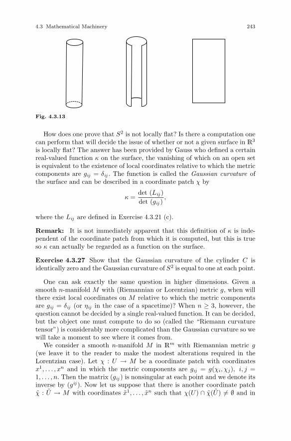
4.3 Mathematical Machinery 243
Fig. 4.3.13
How does one prove that S2 is not locally flat? Is there a computation onecan perform that will decide the issue of whether or not a given surface in R3
is locally flat? The answer has been provided by Gauss who defined a certainreal-valued function κ on the surface, the vanishing of which on an open setis equivalent to the existence of local coordinates relative to which the metriccomponents are gij = δij . The function is called the Gaussian curvature ofthe surface and can be described in a coordinate patch χ by
κ =det (Lij )det (gij )
,
where the Lij are defined in Exercise 4.3.21 (c).
Remark: It is not immediately apparent that this definition of κ is inde-pendent of the coordinate patch from which it is computed, but this is trueso κ can actually be regarded as a function on the surface.
Exercise 4.3.27 Show that the Gaussian curvature of the cylinder C isidentically zero and the Gaussian curvature of S2 is equal to one at each point.
One can ask exactly the same question in higher dimensions. Given asmooth n-manifold M with (Riemannian or Lorentzian) metric g, when willthere exist local coordinates on M relative to which the metric componentsare gij = δij (or ηij in the case of a spacetime)? When n ≥ 3, however, thequestion cannot be decided by a single real-valued function. It can be decided,but the object one must compute to do so (called the “Riemann curvaturetensor”) is considerably more complicated than the Gaussian curvature so wewill take a moment to see where it comes from.
We consider a smooth n-manifold M in Rm with Riemannian metric g(we leave it to the reader to make the modest alterations required in theLorentzian case). Let χ : U → M be a coordinate patch with coordinatesx1, . . . , xn and in which the metric components are gij = g(χi, χj), i, j =1, . . . , n. Then the matrix (gij ) is nonsingular at each point and we denote itsinverse by (gij ). Now let us suppose that there is another coordinate patchχ : U → M with coordinates x1, . . . , xn such that χ(U) ∩ χ(U) �= ∅ and in
244 4 Prologue and Epilogue: The de Sitter Universe
which the metric components gij are gij = δij (so that the line element isds2 = (dx1)2 + · · · + (dxn)2). According to Exercise 4.3.11,
gij =∂xa
∂xi
∂xb
∂xjgab
=∂xa
∂xi
∂xb
∂xjδab
gij =n∑
a=1
∂xa
∂xi
∂xa
∂xj, i, j = 1, . . . , n (4.3.29)
on the intersection. Now, (4.3.29) is equivalent to the matrix equation
(gij ) =(
∂xa
∂xi
)� (∂xa
∂xj
). (4.3.30)
For any invertible matrices A and B,
A = B� B =⇒ A−1 = B−1(B�)−1 =⇒ BA−1 B� = id
so (4.3.30) implies (∂xa
∂xj
)(gij )
(∂xa
∂xi
)�= id.
Written out in detail this gives
∂xa
∂xigij ∂xb
∂xj= δab , a, b = 1, . . . , n. (4.3.31)
Now differentiate (4.3.29) with respect to xk to obtain
∂gij
∂xk=
n∑a=1
(∂xa
∂xj
∂2xa
∂xi∂xk+
∂xa
∂xi
∂2xa
∂xj∂xk
).
Exercise 4.3.28 Write out similar expressions for ∂gik
∂xj and ∂gjk
∂xi and combinethem to get
12
(∂gij
∂xk+
∂gik
∂xj− ∂gjk
∂xi
)=
n∑a=1
∂2xa
∂xj∂xk
∂xa
∂xi. (4.3.32)
Next fix some index b = 1, . . . , n and multiply on both sides of (4.3.32) by
giβ ∂xb
∂xβ(summed over β = 1, . . . , n)

4.3 Mathematical Machinery 245
and then sum over i as required by the summation convention to obtain[12
gβi
(∂gij
∂xk+
∂gik
∂xj− ∂gjk
∂xi
)]∂xb
∂xβ=
n∑a=1
(∂xa
∂xigiβ ∂xb
∂xβ
)∂2xa
∂xj∂xk
=n∑
a=1
δab ∂2xa
∂xj ∂xk
=∂2xb
∂xj∂xk.
Thus,∂2xb
∂xj∂xk= Γβ
jk
∂xb
∂xβ, b, j, k = 1, . . . , n. (4.3.33)
Now fix an index b = 1, . . . , n and let
Jb = (Jb1, . . . , Jbn) =(
∂xb
∂x1, . . . ,
∂xb
∂xn
)be the vector whose components are the entries in the bth row of the Jacobian.Then (4.3.33) can be written
∂Jbj
∂xk= Γβ
jk Jbβ , j, k = 1, . . . , n.
For each j, k, l = 1, . . . , n, we must have
∂2Jbj
∂xl ∂xk=
∂2Jbj
∂xk∂xl
so
∂
∂xl
(Γβ
jk Jbβ
)=
∂
∂xk
(Γβ
jl Jbβ
)Γβ
jk
∂Jbβ
∂xl+
∂Γβjk
∂xlJbβ = Γβ
jl
∂Jbβ
∂xk+
∂Γβjl
∂xkJbβ
Γβjk Γγ
βl Jbγ +∂Γγ
jk
∂xlJbγ = Γβ
jl Γγβk Jbγ +
∂Γγjl
∂xkJbγ(
∂Γγjl
∂xk+ Γβ
jl Γγβk −
∂Γγjk
∂xl− Γβ
jk Γγβl
)Jbγ = 0. (4.3.34)
Now for some notation. For each γ, j, k, l = 1, . . . , n, let
Rγjkl =
∂Γγjl
∂xk+ Γβ
jlΓγβk −
∂Γγjk
∂xl− Γβ
jkΓγβl . (4.3.35)

246 4 Prologue and Epilogue: The de Sitter Universe
Then we can write (4.3.34) as
Rγjkl Jbγ = 0, j, k, l = 1, . . . , n.
We conclude that
Rγjkl
∂xb
∂xγ= 0, b, j, k, l = 1, . . . , n. (4.3.36)
Now, for any fixed j, k, l = 1, . . . , n, (4.3.36) can be regarded as a homoge-neous system of linear equations in
R1jkl , . . . , R
njkl
and, since the Jacobian(
∂xb
∂xγ
)is nonsingular, we conclude that
Rγjkl = 0, γ, j, k, l = 1, . . . , n. (4.3.37)
The conclusion of this long and rather annoying calculation is this. If thereexist coordinates x1, . . . , xn on some open set χ(U) in M relative to whichthe metric components are gij = δij , i, j = 1, . . . , n, then, for any other co-ordinates x1, . . . , xn on some open set χ(U) with χ(U) ∩ χ(U) �= ∅, thefunctions Rγ
jkl of x1, . . . , xn defined by (4.3.35) must vanish identically onχ−1(χ(U) ∩ χ(U)).
Remarkably enough, the converse is also true, in the following sense.Rather than supposing the existence of coordinates x1, . . . , xn with ds2 =(dx1)2 + · · ·+ (dxn)2 and regarding (4.3.29) as a consequence, let us think of
n∑a=1
∂xa
∂xi
∂xa
∂xj= gij , i, j = 1, . . . , n. (4.3.38)
as a system of partial differential equations to be solved for x1, . . . , xn.A solution would provide the transformation equations to a new system ofcoordinates in which gij = δij and it can be shown that a solution existswhenever the “integrability conditions” Rγ
jkl = 0, γ, j, k, l = 1, . . . , n, are sat-isfied (see pages 200–204 of [Sp2], Volume III).
Consequently, the 4n functions Rγjkl defined by (4.3.35) are the replacement
for the Gaussian curvature of a surface in dimensions greater than or equalto 3. These are called the components (relative to χ) of the Riemann curvaturetensor R for M .
Remark: We have not defined the unmodified term “tensor” and will haveno need to do so. However, our experience with 4-tensors in Section 3.1should leave little room for doubt as to the proper definition. Recall thata 4-tensor of contravariant rank 1 and covariant rank 3 can be thought ofas an object described in each admissible frame of reference by 44 = 256

4.3 Mathematical Machinery 247
numbers T abcd , a, b, c, d = 1, 2, 3, 4, with the property that if two admissible
frames are related by xa = Λabx
b, a = 1, 2, 3, 4, then the numbers thatdescribe the 4-tensor in the two frames are related by
T abcd = Λa
α Λbβ Λc
γ Λdδ T α
βγδ,
a, b, c, d = 1, 2, 3, 4. Noting that Λaα = ∂xa
∂xα and Λbβ = ∂xβ
∂xb , etc., this can bewritten
T abcd =
∂xa
∂xα
∂xβ
∂xb
∂xγ
∂xc
∂xδ
∂xdT α
βγδ.
The transformation law for the metric in Exercise 4.3.11 together with a veryhealthy supply of persistence gives an entirely analogous transformation law
Rabcd =
∂xa
∂xα
∂xβ
∂xb
∂xγ
∂xc
∂xδ
∂xdRα
βγδ
for the components of R and it is this transformation law that qualifies R asa “tensor.”
In dimension 4 the Riemann curvature tensor has 44 = 256 components inevery coordinate system, although various symmetries reduce the number ofindependent components to 20. Computing even one of these directly from thedefinition (4.3.35) is, needless to say, an arduous task in general. Nevertheless,everyone should do it once in their lives.
Example 4.3.9 We consider the de Sitter spacetime dS in global coordi-nates x1 = φ1, x2 = φ2, x3 = θ and x4 = tG. The nonvanishing Christoffelsymbols (from Exercise 4.3.22) are
Γ411 = cosh tG sinh tG Γ4
22 = cosh tG sinh tG sin2 φ1
Γ433 = cosh tG sinh tG sin2 φ1 sin2 φ2
Γi4i = Γi
i4 =sinh tGcosh tG
, i = 1, 2, 3
Γ122 = − sin φ1 cosφ1 Γ1
33 = − sinφ1 cosφ1 sin2 φ2
Γ233 = − sin φ2 cosφ2
Γ221 = Γ2
12 = Γ331 = Γ3
13 =cosφ1
sin φ1
Γ332 = Γ3
23 =cosφ2
sin φ2.
We will compute
R4343 =
∂Γ433
∂x4+ Γβ
33Γ4β4 −
∂Γ434
∂x3− Γβ
34Γ4β3.

248 4 Prologue and Epilogue: The de Sitter Universe
First note that
∂Γ433
∂x4=
∂
∂tG(cosh tG sinh tG sin2 φ1 sin2 φ2)
= (cosh2 tG + sinh2 tG) sin2 φ1 sin2 φ2
and∂Γ4
34
∂x3=
∂
∂θ(0) = 0.
Next we have
Γβ33Γ
4β4 = Γ1
33Γ414 + Γ2
33Γ424 + Γ3
33Γ434 + Γ4
33Γ444 = 0
since each Γ4β4 = 0. Finally,
Γβ34Γ
4β3 = Γ1
34Γ413 + Γ2
34Γ423 + Γ3
34Γ433 + Γ4
34Γ443
= 0 + 0 + Γ334Γ
433 + 0
=(
sinh tGcosh tG
)(cosh tG sinh tG sin2 φ1 sin2 φ2)
= sinh2 tG sin2 φ1 sin2 φ2.
Thus,R4
343 = cosh2 tG sin2 φ1 sin2 φ2.
Exercise 4.3.29 Show that, for the de Sitter spacetime in global coordi-nates,
Ri4i4 = −1
for i = 1, 2, 3.
Remark: Observe that, in dS,
δ44g33 − δ4
3g34 = g33 = cosh2 tG sin2 φ1 sin2 φ2 = R4343
(δab = 1 if a = b and 0 if a �= b is just the Kronecker delta). Also,
δiig44 − δi
4g4i = g44 = −1 = Ri4i4
for i = 1, 2, 3. As it happens, one can show that
Rγjkl = δγ
kgjl − δγl gjk (4.3.39)
for all γ, i, j, k = 1, 2, 3, 4. Thus, for example, setting k = γ and summingover γ gives
Rγjγl = δγ
γgjl − δγl gjγ = 4gjl − gjl = 3gjl .
Remark: A manifold M with metric g is said to have constant (sectional)curvature if there is a constant K such that
Rγjkl = K (δγ
kgjl − δγl gjk )
4.4 The de Sitter Universe dS 249
in any local coordinate system. de Sitter spacetime dS therefore has constantcurvature K = 1. We will encounter this notion again in the next section.
The Riemann curvature tensor contains all of the information about amanifold’s local deviations from “flatness” and, in the case of a spacetime,this is precisely what we mean by a gravitational field (see Section 4.1). It is,however, a rather cumbersome creature and one can often make due (bothmathematically and physically) with somewhat simpler objects that we nowintroduce. For any n-manifold M with (Riemannian or Lorentzian) metric gwe define, in any local coordinate system on M , the components of the Riccitensor Rij by
Rij = Rγiγj (sum over γ = 1, . . . , n)
for i, j = 1, . . . , n. The scalar curvature R of M is then defined by
R = gij Rij (sum over i, j = 1, . . . , n).
According to the previous Remark, the Ricci tensor of de Sitter spacetimedS is
Rij = 3gij
and soR = gijRij = gij (3gij) = 3gijgji = 3δj
j = 3(4) = 12.
Remark: The scalar curvature is generally a real-valued function on M ,but in the case of dS happens to be a constant function.
Finally, we define, in any local coordinate system for M , the components ofthe Einstein tensor Gij by
Gij = Rij −12
Rg ij
for i, j = 1, . . . , n. Thus, for dS,
Gij = 3gij −12(12) gij = −3gij .
Exercise 4.3.30 Show that Gij = 0 for all i, j = 1, . . . , n if and only ifRij = 0 for all i, j = 1, . . . , n. Hint: Assuming Gij = 0, consider gijGij .
4.4 The de Sitter Universe dS
A spacetime, as we have defined it, is a 4-dimensional manifold with a Lorentzmetric. The motivation behind the definition was an attempt to model theevent world when gravitational effects cannot be regarded as negligible. Itis certainly not the case, however, that every spacetime represents some

250 4 Prologue and Epilogue: The de Sitter Universe
physically realistic gravitational field. Einstein’s idea was that the space-time should be “determined” by the mass-energy distribution giving rise tothe gravitational field and he struggled for many years to arrive at equationsthat specified just how the latter determined the former. The end result ofthe struggle was a set of ten coupled nonlinear partial differential equationsfor the metric components gij called the Einstein field equations. It is withthese that the general theory of relativity begins and we will not be so boldas to offer a precis of their derivation. We simply record the equations, makea few unremarkable observations and then move on to their relevance to ourstory. A spacetime M with Lorentz metric g is said to satisfy the Einsteinfield equations if, in any local coordinate system,
Rij −12Rg ij + Λgij = 8πTij , i, j = 1, 2, 3, 4, (4.4.1)
where Rij − 12
Rg ij = Gij is the Einstein tensor, Λ is a constant, called thecosmological constant, and Tij is called the energy-momentum tensor and isa direct analogue of the energy-momentum transformation for the electro-magnetic field on Minkowski spacetime that we introduced in Section 2.5.The role of Tij is to describe the mass-energy distribution giving rise to thegravitational field being modeled by gij . The equations relate the geometryof the spacetime, described by the left-hand side, to the mass-energy distri-bution, described by the right-hand side. Together with the so-called geodesichypothesis that free particles have worldlines in M that are timelike or nullgeodesics, (4.4.1) contains essentially the entire content of general relativity.
The left-and right-hand sides of (4.4.1) have the same transformation law
to a new system of local coordinates(
Fij =∂xk
∂xi
∂xl
∂xjFkl
)so, if they are
satisfied for one set of charts covering M , they are satisfied in any coordinatesystem (they are “tensor equations”). In particular, it makes sense to definean empty space solution to Einstein’s equations to be a spacetime satisfying(4.4.1) with Tij = 0, i, j = 1, 2, 3, 4.
Exercise 4.4.1 Show that the de Sitter spacetime dS is an empty spacesolution to the Einstein equations with Λ = 3.
Remark: It may strike the reader as peculiar that we introduce “emptyspace solutions” since our motivation has been to model nontrivial gravita-tional fields. Let us explain. When Λ = 0 the empty space equations areGij = 0 which, by Exercise 4.3.30, are the same as
Rij = 0. (4.4.2)
Manifolds satisfying (4.4.2) are said to be Ricci flat and, in general relativ-ity, they are regarded as an analogue of the source free Maxwell equationsintroduced in Section 2.7. Solutions describe gravitational fields in regions ofspacetime in which the mass-energy giving rise to the field is “elsewhere.”
4.4 The de Sitter Universe dS 251
The best known example is the Schwarzschild solution describing the fieldexterior to a spherically symmetric mass/star (see Chapter Six of [Wald]).On the other hand, when Λ �= 0, the empty space equations are
Gij + Λgij = 0 (4.4.3)
and here the interpretation is more subtle. One might, for example, rewrite(4.4.3) as
Gij = 8π
(− Λ
8πgij
)(4.4.4)
and regardT vac
ij = − Λ8π
gij (4.4.5)
as an energy-momentum tensor for some unspecified mass-energy distributionand (4.4.4) as the Einstein equations with cosmological constant zero. In thisinterpretation, (4.4.5) is often thought of as the energy-momentum of the vac-uum, due perhaps to quantum fluctuations of the vacuum state required byquantum field theory. In this guise, T vac
ij is often attributed to what has cometo be called “dark energy.” Alternatively, one could simply regard the cosmo-logical term Λgij in Einstein’s equations (4.4.1) as a necessary ingredient inthe basic laws of physics, independent of any mass-energy interpretation. Inthis case one has solutions like dS representing a genuinely “empty” universe,but which are, nevertheless, not flat (dS has nonzero curvature tensor). Suchsolutions therefore represent alternatives to Minkowski spacetime with verydifferent mathematical and, as we shall see, physical properties.
It is not the usual state of affairs, of course, to be given a spacetime and anenergy-momentum tensor and be asked to check (as in Exercise 4.4.1) thattogether they give a solution to the Einstein equations. Rather, one wouldbegin with some physical distribution of matter and energy (an electromag-netic field, a single massive object such as a star, or an entire universe fullof galaxies) and one would attempt to solve the equations (4.4.1) for themetric. Aside from the enormous complexity of the equations (express Rij
and R directly in terms of gij and substitute into (4.4.1)) there are subtletiesin this that may not be apparent at first glance. The Einstein equations arewritten in coordinates, but coordinates on what? The objective is to con-struct the manifold and its metric so neither can be regarded as given tous. To solve (4.4.1) one must begin with a guess (physicists prefer the term“ansatz”) based on one’s physical intuition concerning the field being mod-eled as to what at least one coordinate patch on the sought after manifoldmight look like. Even if one should succeed in this, the end result will be nomore than a local expression for the metric in one coordinate system; therest of the manifold is still hidden from view. Moreover, it is the metric it-self that determines the spacetime measurements in the manifold. Since onecannot describe energy and momentum without reference to space and timemeasurements, even Tij cannot be regarded as given, but depends on the un-known metric components gij . Even the true physical meaning of the ansatzcoordinates cannot be known until after the equations are solved.
252 4 Prologue and Epilogue: The de Sitter Universe
All of these subtleties add spice to the problem of solving the Einsteinequations, but this is not really our concern here. We would, however, like tosay a few words about the ansatz appropriate to what are called cosmologicalmodels (spacetimes intended to model the global structure of the universe asa whole). For this we need just one more mathematical tool.
Let M1 and M2 be two smooth manifolds and F : M1 → M2 a smoothmap. At each point p ∈ M , we define the derivative F∗p of F at p to bethe map
F∗p : Tp(M1) → TF (p) (M2)
that carries the velocity vector of a smooth curve α in M1 through p to thevelocity vector of its image F ◦ α under F , i.e.,
F∗p(α′ (t0)) = (F ◦ α)′ (t0).
In this way smooth maps carry tangent vectors in the domain to tangentvectors in the range. Now suppose M1 and M2 have metrics g1 and g2, re-spectively (both Riemannian or both Lorentzian) and that F : M1 → M2 isa diffeomorphism. Then F is called an isometry if it preserves inner productsat each point, i.e., if
g1(α′ (t0), β′ (t1)) = g2 ((F ◦ α)′ (t0), (F ◦ β)′ (t1))
for all smooth curves α and β in M1 with α(t0) = β(t1). In particular,an isometry of a manifold M with metric onto itself is the analogue of anorthogonal transformation of a vector space with inner product onto itself. Inparticular, the collection of all such form a group, called the isometry groupof M . For dS this group is precisely the set of restrictions to dS of orthogonaltransformations of M5 and is called the de Sitter group (this result is notobvious, but we do not need it and so will not prove it). For spacetimes,isometries are our new Lorentz transformations.
The two most basic physical assumptions that go into the construction of acosmological model in general relativity are called “spatial homogeneity” and“spatial isotropy.” Intuitively, these assert that, at any “instant”, all pointsand all directions in “space” should “look the same.” Since “instant” and“space” are the very things that relativity forbids us ascribing a meaning toindependent of some observer, it is not so clear what this is supposed to mean.We will attempt a somewhat more precise statement of what is intended. Aspacetime M is said to be spatially homogeneous and isotropic if the followingconditions are satisfied (see Figure 4.4.1).
(A) There exists a family of free observers (future-directed, timelikegeodesics) with worldlines filling all of M (for each p ∈ M there existsone and only one of these geodesics αp with αp(tp) = p for some valuetp of proper time on αp.
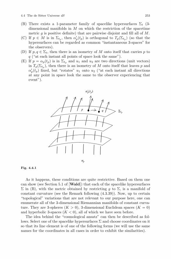
4.4 The de Sitter Universe dS 253
(B) There exists a 1-parameter family of spacelike hypersurfaces Σt (3-dimensional manifolds in M on which the restriction of the spacetimemetric g is positive definite) that are pairwise disjoint and fill all of M .
(C) If p ∈ M is in Σtp , then α′p(tp) is orthogonal to Tp(Σtp) (so that the
hypersurfaces can be regarded as common “instantaneous 3-spaces” forthe observers).
(D) If p, q ∈ Σt, then there is an isometry of M onto itself that carries p toq (“at each instant all points of space look the same”).
(E) If p = αp(tp) is in Σtp and u1 and u2 are two directions (unit vectors)in Tp(Σtp), then there is an isometry of M onto itself that leaves p andα′
p(tp) fixed, but “rotates” u1 onto u2 (“at each instant all directionsat any point in space look the same to the observer experiencing thatevent”).
ap(tp)
p
ap
q Σtp
Fig. 4.4.1
As it happens, these conditions are quite restrictive. Based on them onecan show (see Section 5.1 of [Wald]) that each of the spacelike hypersurfacesΣ in (B), with the metric obtained by restricting g to Σ, is a manifold ofconstant curvature (see the Remark following (4.3.39)). Now, up to certain“topological” variations that are not relevant to our purpose here, one canenumerate all of the 3-dimensional Riemannian manifolds of constant curva-ture. They are 3-spheres (K > 0), 3-dimensional Euclidean spaces (K = 0)and hyperbolic 3-spaces (K < 0), all of which we have seen before.
The idea behind the “cosmological ansatz” can then be described as fol-lows. Select one of the spacelike hypersurfaces Σ and choose coordinates on itso that its line element is of one of the following forms (we will use the samenames for the coordinates in all cases in order to exhibit the similarities).
254 4 Prologue and Epilogue: The de Sitter Universe
dψ2 + sin2 ψ(dφ2 + sin2 φ dθ2) (Σ = S3)
dψ2 + ψ2(dφ2 + sin2 φdθ2) (Σ = R3)
dψ2 + sinh2 ψ(dφ2 + sin2 φ dθ2) (Σ = H3(1))
Each of our free observers has a worldline that intersects Σ at, without lossof generality, t = 0. Now “move” the coordinates of Σ along these worldlinesby fixing each observer’s spatial coordinates ψ, φ, θ at the values they haveat t = 0 on Σ and taking the fourth coordinate of each event to be the propertime t of the observer that experiences that event. Allowing the “scale” of thespatial cross sections to (perhaps) vary with t and recalling that the observerworldlines are orthogonal to these cross sections we conclude that, in thesecoordinates, the line element of M should have one of the forms
−dt2 + a2(t)
⎧⎪⎨⎪⎩dψ2 + sin2 ψ(dφ2 + sin2 φdθ2)
dψ2 + ψ2(dφ2 + sin2 φdθ2)
dψ2 + sinh2 ψ(dφ2 + sin2 φdθ2)
where a(t) is some positive function of t. These are called Robertson-Walkermetrics and our conclusion (or, rather, now our ansatz) is that a spatiallyhomogeneous and isotropic spacetime should admit coordinate systems inwhich the spacetime metric g assumes one of these forms.
If we were in the business of doing cosmology (which we are not) wewould choose one of these, substitute into the Einstein equations (for somechoice of Λ and some Tij ) and determine the scale function a(t). Our inter-est in the Robertson-Walker metrics is that we have seen them all beforeand all in the same place. Indeed, except for the names of the variables,the metric for dS in global coordinates given by (4.3.22) is the Robertson-Walker metric with spherical spatial cross sections and a(t) = cosh t; inplanar coordinates, Exercise 4.3.19 gives the same metric as a Robertson-Walker metric with flat spatial cross sections and a(t) = e2t; in hyperboliccoordinates, Exercise 4.3.20 exhibits the metric of dS as a Robertson-Walker metric with spatial cross sections that are hyperbolic 3-spaces anda(t) = sinh t. These three represent very different physical situations, ofcourse, but they are all simply different descriptions of the same underlyingspacetime (or a part of it).
It is certainly interesting, but perhaps not so terribly surprising thatentirely different physical pictures of the universe can be modeled in a sin-gle spacetime. Certain things about a spacetime manifold are “absolute”,i.e., independent of observer. The geodesics, for example, and the Riemanncurvature tensor, as well as the causality relations between events are all de-termined entirely by the manifold and its metric. However, a spacetime suchas dS admits many families of timelike geodesics filling the manifold (e.g., thetG−, tp−, and tH–coordinate curves), each with as much right as the other toclaim for itself the title of “cosmic observer” and determine its own “instan-taneous 3-spaces.” This is entirely analogous to the situation in Minkowski

4.5 Infinity in Minkowski and de Sitter Spacetimes 255
spacetime where different admissible observers disagree as to which sets ofevents count as instantaneous 3-spaces (although in this case they all agreethat “space” is R3).
Perhaps more interesting is the fact that all of these various observers agreethat they are in an empty universe (Exercise 4.4.1), not unlike an admissibleobserver in Minkowski spacetime, but they see the world quite differentlythan their Minkowskian colleague. Aside from the fact that they may see“space” as spherical or hyperbolic, they also see it as expanding (indeed,expanding at an exponentially increasing rate) due to the presence of thescale factors a(t) = cosh t, e2t, and sinh t. Any two observers in the familyof cosmic observers have fixed spatial coordinates, but even so their spatialseparation is increasing exponentially with t (in the spherical case one mightpicture a balloon being blown up). Remarkably enough, recent astronomicalobservations suggest that the expansion of our universe is, indeed, accelerat-ing and this has prompted a renewed interest in the de Sitter universe as apotential alternative to Minkowski spacetime (see, for example, [CGK]). Aswe have seen, these two models of the empty universe have quite differentproperties and we will conclude by describing yet one more such property,this one related to the asymptotic behavior of worldlines.
4.5 Infinity in Minkowski and de Sitter Spacetimes
We propose to offer a precise definition of “infinity” in both Minkowski andde Sitter spacetimes and then show how the two differ in the behavior oftheir timelike and null curves “at infinity.” This will lead to the notions ofparticle and event “horizons” in dS that do not exist in M (since we are nowregarding Minkowski spacetime as a Lorentzian manifold it would probablybe more appropriate to call it R3,1, but we’ll stick with M). The idea behindall of this is due to Roger Penrose and amounts to “squeezing” both M and dSinto finite regions of yet another spacetime in such a way that the boundariesof these regions can be identified with “infinity” in M and dS. The spacetimeinto which we squeeze them is, moreover, of considerable significance, at leasthistorically. It is called the Einstein static universe and we shall denote it E .
Remark: Here, very briefly, is the story of E . As Einstein originally pro-posed them, the field equations did not contain a cosmological constant (theywere our (4.4.1) with Λ = 0). Einstein applied these equations to a spatiallyhomogeneous and isotropic universe with S3 spatial cross sections and filledwith a uniform “dust” of galaxies (Tij was the energy-momentum tensor forwhat is called a perfect fluid with zero pressure). He found, much to his cha-grin, that the solution described an expanding universe. He was chagrined bythis because, at the time, there was no reason to believe that the universewas anything but what it had been assumed for centuries to be, that is, fixed

256 4 Prologue and Epilogue: The de Sitter Universe
and immutable. He then, very reluctantly, modified his field equations by in-cluding the cosmological term Λgij because he could then, for a very specificchoice of Λ, find a static solution E . Then, of course, along came Edwin Hub-ble who interpreted the observed redshift of light from distant galaxies as aDoppler shift and concluded that the universe is, in fact, expanding. Einstein(and almost everyone else) then abandoned E along with the cosmologicalconstant that gave rise to it. As we have seen however, there may be reasonto resurrect Λ and there are those who believe that E also deserves a reprieve(see [DS]).
Our first task then is to construct the spacetime into which we will squeezeM and dS. Since E can be described in terms very much like those with whichwe described dS we will leave some of the details to the reader. As a set, Econsists of those points (u1, u2, u3, u4, u5) in R5 satisfying
(u1)2 + (u2)2 + (u3)2 + (u4)2 = 1
and so is pictured as a cylinder setting on the 3-sphere in R5.
Exercise 4.5.1 Show that E is diffeomorphic to S3 × R (and thereforeto dS ).
Now define a map from R4 to R5 by
u1 = sin φ1 cos φ2
u2 = sin φ1 sin φ2 cos θ
u3 = sin φ1 sin φ2 sin θ (4.5.1)
u4 = cos φ1
u5 = tE .
Exercise 4.5.2 Show that the image of the map (4.5.1) is all of E and thateach point in E is contained in an open subset of E on which the inverse ofthe map is a chart.
Thus, with the usual caveat regarding appropriate ranges for the variables,(φ1, φ2, θ, tE) are global coordinates on E . In Figure 4.5.1 the cylinder Eis represented by suppressing the coordinates φ2 and θ and regarding φ1 asan angular coordinate on a copy of S1 in S3 (more precisely, Figure 4.5.1represents a slice of E obtained by holding φ2 and θ fixed).
Exercise 4.5.3 Restrict the M5-inner product to each tangent spaceTp(E), p ∈ E , and show that the corresponding line element in (φ1, φ2, θ, tE)-coordinates is
ds2 = dφ12 + sin2 φ1
(dφ2
2 + sin2 φ2 dθ2)− dt2
E . (4.5.2)
Remark: The reader may wish to pause and compare (4.5.2) with the resultof Exercise 4.3.18. We will have more to say about this shortly. It should also
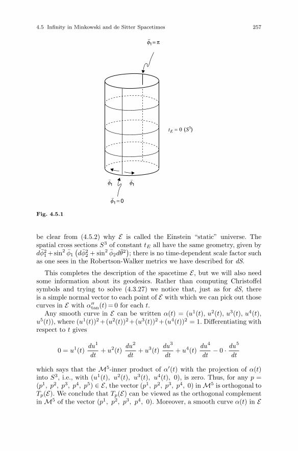
4.5 Infinity in Minkowski and de Sitter Spacetimes 257
−f1−f1
−f1 = 0
−f1 = π
tE = 0 (S3)
Fig. 4.5.1
be clear from (4.5.2) why E is called the Einstein “static” universe. Thespatial cross sections S3 of constant tE all have the same geometry, given bydφ2
1 +sin2 φ1
(dφ2
2 + sin2 φ2dθ2); there is no time-dependent scale factor such
as one sees in the Robertson-Walker metrics we have described for dS.
This completes the description of the spacetime E , but we will also needsome information about its geodesics. Rather than computing Christoffelsymbols and trying to solve (4.3.27) we notice that, just as for dS, thereis a simple normal vector to each point of E with which we can pick out thosecurves in E with α′′
tan(t)= 0 for each t.Any smooth curve in E can be written α(t) = (u1(t), u2(t), u3(t), u4(t),
u5(t)), where (u1(t))2 +(u2(t))2 +(u3(t))2 +(u4(t))2 = 1. Differentiating withrespect to t gives
0 = u1(t)du1
dt+ u2(t)
du2
dt+ u3(t)
du3
dt+ u4(t)
du4
dt− 0 · du5
dt
which says that the M5-inner product of α′(t) with the projection of α(t)into S3, i.e., with (u1(t), u2(t), u3(t), u4(t), 0), is zero. Thus, for any p =(p1, p2, p3, p4, p5) ∈ E , the vector (p1, p2, p3, p4, 0) in M5 is orthogonal toTp(E). We conclude that Tp(E) can be viewed as the orthogonal complementin M5 of the vector (p1, p2, p3, p4, 0). Moreover, a smooth curve α(t) in E
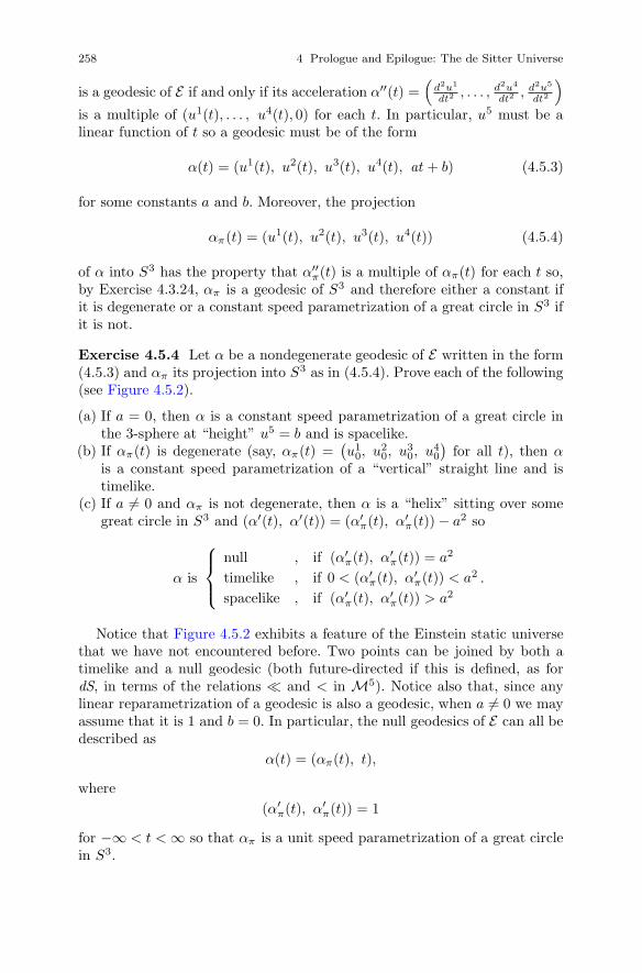
258 4 Prologue and Epilogue: The de Sitter Universe
is a geodesic of E if and only if its acceleration α′′(t) =(
d2u1
dt2, . . . , d2u4
dt2, d2u5
dt2
)is a multiple of (u1(t), . . . , u4(t), 0) for each t. In particular, u5 must be alinear function of t so a geodesic must be of the form
α(t) = (u1(t), u2(t), u3(t), u4(t), at + b) (4.5.3)
for some constants a and b. Moreover, the projection
απ(t) = (u1(t), u2(t), u3(t), u4(t)) (4.5.4)
of α into S3 has the property that α′′π(t) is a multiple of απ(t) for each t so,
by Exercise 4.3.24, απ is a geodesic of S3 and therefore either a constant ifit is degenerate or a constant speed parametrization of a great circle in S3 ifit is not.
Exercise 4.5.4 Let α be a nondegenerate geodesic of E written in the form(4.5.3) and απ its projection into S3 as in (4.5.4). Prove each of the following(see Figure 4.5.2).
(a) If a = 0, then α is a constant speed parametrization of a great circle inthe 3-sphere at “height” u5 = b and is spacelike.
(b) If απ(t) is degenerate (say, απ(t) =(u1
0, u20, u3
0, u40
)for all t), then α
is a constant speed parametrization of a “vertical” straight line and istimelike.
(c) If a �= 0 and απ is not degenerate, then α is a “helix” sitting over somegreat circle in S3 and (α′(t), α′(t)) = (α′
π(t), α′π(t)) − a2 so
α is
⎧⎪⎨⎪⎩null , if (α′
π(t), α′π(t)) = a2
timelike , if 0 < (α′π(t), α′
π(t)) < a2
spacelike , if (α′π(t), α′
π(t)) > a2
.
Notice that Figure 4.5.2 exhibits a feature of the Einstein static universethat we have not encountered before. Two points can be joined by both atimelike and a null geodesic (both future-directed if this is defined, as fordS, in terms of the relations � and < in M5). Notice also that, since anylinear reparametrization of a geodesic is also a geodesic, when a �= 0 we mayassume that it is 1 and b = 0. In particular, the null geodesics of E can all bedescribed as
α(t) = (απ(t), t),
where(α′
π(t), α′π(t)) = 1
for −∞ < t < ∞ so that απ is a unit speed parametrization of a great circlein S3.
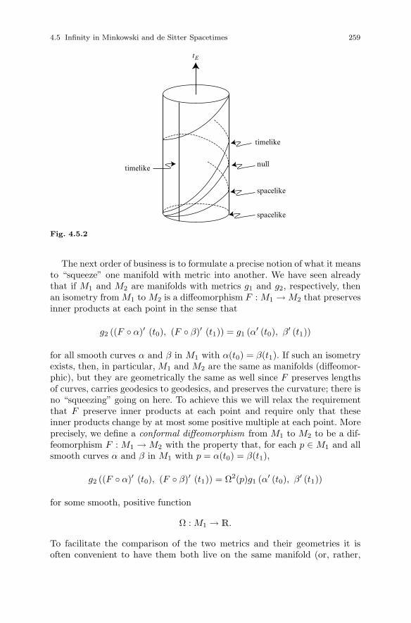
4.5 Infinity in Minkowski and de Sitter Spacetimes 259
tE
spacelike
timelike
timelike
spacelike
null
Fig. 4.5.2
The next order of business is to formulate a precise notion of what it meansto “squeeze” one manifold with metric into another. We have seen alreadythat if M1 and M2 are manifolds with metrics g1 and g2, respectively, thenan isometry from M1 to M2 is a diffeomorphism F : M1 → M2 that preservesinner products at each point in the sense that
g2 ((F ◦ α)′ (t0), (F ◦ β)′ (t1)) = g1 (α′ (t0), β′ (t1))
for all smooth curves α and β in M1 with α(t0) = β(t1). If such an isometryexists, then, in particular, M1 and M2 are the same as manifolds (diffeomor-phic), but they are geometrically the same as well since F preserves lengthsof curves, carries geodesics to geodesics, and preserves the curvature; there isno “squeezing” going on here. To achieve this we will relax the requirementthat F preserve inner products at each point and require only that theseinner products change by at most some positive multiple at each point. Moreprecisely, we define a conformal diffeomorphism from M1 to M2 to be a dif-feomorphism F : M1 → M2 with the property that, for each p ∈ M1 and allsmooth curves α and β in M1 with p = α(t0) = β(t1),
g2 ((F ◦ α)′ (t0), (F ◦ β)′ (t1)) = Ω2(p)g1 (α′ (t0), β′ (t1))
for some smooth, positive function
Ω : M1 → R.
To facilitate the comparison of the two metrics and their geometries it isoften convenient to have them both live on the same manifold (or, rather,
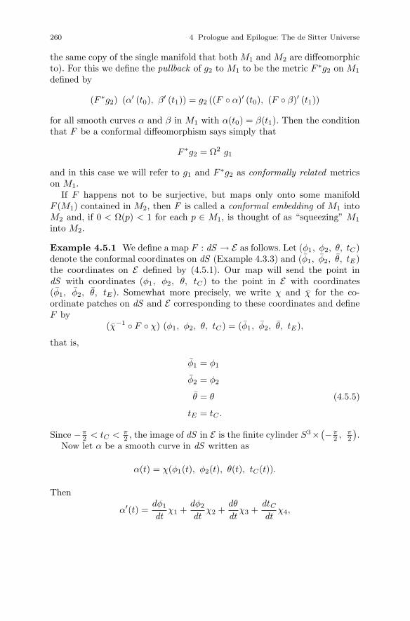
260 4 Prologue and Epilogue: The de Sitter Universe
the same copy of the single manifold that both M1 and M2 are diffeomorphicto). For this we define the pullback of g2 to M1 to be the metric F ∗g2 on M1
defined by
(F ∗g2) (α′ (t0), β′ (t1)) = g2 ((F ◦ α)′ (t0), (F ◦ β)′ (t1))
for all smooth curves α and β in M1 with α(t0) = β(t1). Then the conditionthat F be a conformal diffeomorphism says simply that
F ∗g2 = Ω2 g1
and in this case we will refer to g1 and F ∗g2 as conformally related metricson M1.
If F happens not to be surjective, but maps only onto some manifoldF (M1) contained in M2, then F is called a conformal embedding of M1 intoM2 and, if 0 < Ω(p) < 1 for each p ∈ M1, is thought of as “squeezing” M1
into M2.
Example 4.5.1 We define a map F : dS → E as follows. Let (φ1, φ2, θ, tC)denote the conformal coordinates on dS (Example 4.3.3) and (φ1, φ2, θ, tE)the coordinates on E defined by (4.5.1). Our map will send the point indS with coordinates (φ1, φ2, θ, tC) to the point in E with coordinates(φ1, φ2, θ, tE). Somewhat more precisely, we write χ and χ for the co-ordinate patches on dS and E corresponding to these coordinates and defineF by
(χ−1 ◦ F ◦ χ) (φ1, φ2, θ, tC) = (φ1, φ2, θ, tE),
that is,
φ1 = φ1
φ2 = φ2
θ = θ (4.5.5)
tE = tC .
Since −π2 < tC < π
2 , the image of dS in E is the finite cylinder S3×(−π
2 , π2
).
Now let α be a smooth curve in dS written as
α(t) = χ(φ1(t), φ2(t), θ(t), tC(t)).
Then
α′(t) =dφ1
dtχ1 +
dφ2
dtχ2 +
dθ
dtχ3 +
dtC
dtχ4,
4.5 Infinity in Minkowski and de Sitter Spacetimes 261
where each χi is evaluated at α(t). Moreover,
(F ◦ α) (t) = (F ◦ χ) (φ1(t), φ2(t), θ(t), tC(t))
= χ((χ−1 ◦ F ◦ χ) (φ1(t), φ2(t), θ(t), tC(t))
)= χ(φ1(t), φ2(t), θ(t), tE(t))
so
(F ◦ α)′(t) =dφ1
dtχ1 +
dφ2
dtχ2 +
dθ
dtχ3 +
dtE
dtχ4
=dφ1
dtχ1 +
dφ2
dtχ2 +
dθ
dtχ3 +
dtC
dtχ4
= F∗α(t) (α′(t)),
where each χi is evaluated at F (α(t)). In particular,
F∗p(χi(p)) = χi(F (p)), i = 1, 2, 3, 4.
Writing gE for the restriction to S3×(−π
2 , π2
)⊆ E of the metric on E given by
(4.5.2) we compute the components of F ∗gE in conformal coordinates on dS.
(F ∗gE) (χi(p), χj(p)) = gE(F∗p(χi(p)), F∗p(χj(p))
)= gE(χi(F (p)), χj(F (p)))
=
⎧⎪⎪⎪⎪⎪⎪⎨⎪⎪⎪⎪⎪⎪⎩
0 , i �= j
1 , i = j = 1sin2 φ1(F (p)) , i = j = 2sin2 φ1(F (p)) sin2 φ2(F (p)) , i = j = 3−1 , i = j = 4
=
⎧⎪⎪⎪⎪⎪⎪⎨⎪⎪⎪⎪⎪⎪⎩
0 , i �= j
1 , i = j = 1sin2 φ1(p) , i = j = 2sin2 φ1(p) sin2 φ2(p) , i = j = 3−1 , i = j = 4
Consequently, the line element for the metric F ∗gE on dS in conformal coor-dinates (φ1, φ2, θ, tC) is
dφ21 + sin2 φ1
(dφ2
2 + sin2 φ2 dθ2)− dt2
C
and this, according to Exercise 4.3.18, is cos2 tC times the line element forthe metric gdS of dS in conformal coordinates. We conclude therefore that
F ∗gE = Ω2gdS
262 4 Prologue and Epilogue: The de Sitter Universe
where Ω(φ1, φ2, θ, tC) = cos tC . Thus, F ∗gE and gdS are conformally relatedmetrics on dS or, said otherwise, F is a conformal embedding of dS into E .
We will have more to say about this particular example shortly, but firstwe will need to develop a few general results on conformally related metrics.First observe that a conformal diffeomorphism of one spacetime manifold toanother carries spacelike, timelike and null curves onto curves of the sametype since
g2((F ◦ α)′ (t), (F ◦ α)′ (t)) = Ω2 (α(t)) g1 (α′ (t), α′ (t))
so the causal character of the tangent vector is preserved at each point. It isnot the case, however, that conformal diffeomorphisms always carry geodesicsonto geodesics. However, we will show that a conformal diffeomorphism ona spacetime manifold carries a null geodesic onto a (reparametrization of a)null geodesic.
We begin by having another look at the geodesic equations
d2xr
dt2+ Γr
ij
dx i
dtdx j
dt= 0, r = 1, . . . , n (4.5.6)
in an n-manifold M with metric g. We recall (Lemma 4.3.1) that thesegeodesic equations are not independent of parametrization. Indeed, a geodesicmust be parametrized in a very particular way in order for its coordinatefunctions to satisfy (4.5.6). These are called affine parametrizations and theydiffer from each other by simple linear functions. Of course, any curve can bereparametrized anyway you like and we would like to see what the geodesicequations look like in an arbitrary parametrization. Thus, we assume that(4.5.6) is satisfied and introduce a reparametrization t = h(s), where h issome smooth function with h′(s) > 0 for all s. Then
dxa
ds=
dxa
dtdtds
d2xa
ds2 =d2xa
dt2
(dtds
)2
+dxa
dtd2t
ds2
and so
d2xr
ds2 + Γrij
dx i
dsdx j
ds=
d2xr
dt2
(dtds
)2
+dx r
dtd2t
ds2 + Γrij
dx i
dtdx j
dt
(dtds
)2
=(
dtds
)2(
d2xr
dt2 + Γrij
dx i
dtdx j
dt
)+
dx r
dtd2t
ds2
=d2t
ds2
dx r/dsdt/ds
4.5 Infinity in Minkowski and de Sitter Spacetimes 263
d2xr
ds2 + Γrij
dx i
dsdx j
ds=(
d2t/ds2
dt/ds
)dx r
ds, r = 1, . . . , n. (4.5.7)
Thus, (4.5.7) are the equations satisfied by a geodesic when expressed interms of an arbitrary parameter s. Of course, when s is a linear function ofthe affine parameter t, they reduce to (4.5.6).
Notice that if we are given some smooth curve α(s) in M that satisfies
d2xr
ds2 + Γrij
dx i
dsdx j
ds= f(s)
dx r
ds, r = 1, . . . , n (4.5.8)
for some function f(s), we can introduce a parameter t by setting
d2t/ds2
dt/ds= f(s)
and solved2t
ds2 − f(s)dtds
= 0
to obtaindtds
= e∫
sa
f(ξ)dξ
where a is an arbitrary constant. Reparametrized in terms of t, α(t) satisfies(4.5.6) and is therefore a geodesic of M . We will write out a specific exampleshortly, but first we use this to show that if α(t) is a null geodesic in aspacetime manifold M (with affine parameter t), then α(t) is also a nullgeodesic in any conformally related metric, although t need not be an affineparameter for it. Thus, conformal diffeomorphisms preserve null geodesics, upto parametrization. For the proof we will first need to compute the Christoffelsymbols of a conformally related metric.
We let M denote an n-manifold with metric g and suppose g = Ω2g is aconformally related metric on M . In any coordinate system x1, . . . , xn themetric components are gij and gij = Ω2gij and the entries of the inversematrices are related by gij = Ω−2gij . By definition, the Christoffel symbolsfor g in these coordinates are
Γrij =
12grk
(∂gik
∂xj+
∂gjk
∂xi− ∂gij
∂xk
), r, i, j = 1, . . . , n

264 4 Prologue and Epilogue: The de Sitter Universe
and those for g are
Γrij =
12grk
(∂gik
∂xj+
∂gjk
∂xi− ∂gij
∂xk
)=
12
Ω−2 grk
(∂
∂xj
(Ω2 gik
)+
∂
∂xi
(Ω2 gjk
)− ∂
∂xk
(Ω2 gij
))=
12
Ω−2 grk
(Ω2 ∂gik
∂xj+ 2Ω
∂Ω∂xj
gik +
Ω2 ∂gjk
∂xi+ 2Ω
∂Ω∂xi
gjk −
Ω2 ∂gij
∂xk− 2Ω
∂Ω∂xk
gij
)= Γr
ij + Ω−1
(∂Ω∂xj
grkgik +∂Ω∂xi
grkgik − ∂Ω∂xk
grkgij
)= Γr
ij + Ω−1
(δri
∂Ω∂xj
+ δrj
∂Ω∂xi
− grkgij∂Ω∂xk
).
Thus,
Γrij = Γr
ij + δri
∂
∂xj(ln Ω) + δr
j
∂
∂xi(ln Ω) − grkgij
∂
∂xk(ln Ω). (4.5.9)
Next we consider a curve α(t) in a spacetime M that is null relative to g,and therefore also relative to g. Thus,
gijdx i
dtdx j
dt= 0 (4.5.10)
for all t. We claim that (4.5.10) implies
d2xr
dt2+ Γr
ij
dx i
dtdx j
dt=
d2xr
dt2+ Γr
ij
dx i
dtdx j
dt+
d
dt(2 ln Ω)
dx r
dt(4.5.11)
for r = 1, 2, 3, 4. Indeed, multiplying (4.5.9) by dx i
dtdx j
dtand summing as indi-
cated gives
Γrij
dx i
dtdx j
dt− Γr
ij
dx i
dtdx j
dt
= δri
∂
∂xj(ln Ω)
dx i
dtdx j
dt+ δr
j
∂
∂xi(ln Ω)
dx i
dtdx j
dt
− grk ∂
∂xk(ln Ω) gij
dx i
dtdx j
dt
=
(∂
∂xj(ln Ω)
dx i
dt+
∂
∂xi(ln Ω)
dx i
dt
)dx r
dt− 0
4.5 Infinity in Minkowski and de Sitter Spacetimes 265
=
(2
∂
∂xi(ln Ω)
dx i
dt
)dx r
dt
=(
2d
dt(ln Ω)
)dx r
dt
from which (4.5.11) is immediate.Now we can fulfill our promise about null geodesics. Suppose that α(t) is
a null geodesic of g with affine parameter t. Then (4.5.10) is satisfied and,moreover,
d2xr
dt2+ Γr
ij
dx i
dtdx j
dt= 0, r = 1, 2, 3, 4.
Thus, (4.5.11) gives
d2xr
dt2+ Γr
ij
dx i
dtdx j
dt=
d
dt(2 lnΩ)
dx r
dt, (4.5.12)
for r = 1, 2, 3, 4. It follows from (4.5.8) that α(t) is also a (null) geodesic of g,but that t is not an affine parameter for it. From the discussion immediatelyfollowing (4.5.8) we can introduce an affine parameter μ for this null geodesicof g by
dμ
dt= exp
(∫ t
a
d
dξ(2 ln Ω)dξ
).
Taking the multiplicative constant to be one,
dμ
dt= Ω2
(x1(t), . . . , x4(t)
)(4.5.13)
so μ(t) can be found by integration.
Example 4.5.2 We return to the conformally related metrics gdS andF ∗gE on dS discussed in Example 4.5.1. Here F ∗gE = Ω2gdS , whereΩ(φ1, φ2, θ, tC) = cos tC . Every null geodesic in dS (relative to gdS ) canbe described as follows.
Fix a point p ∈ dS and a null vector v in M5 orthogonal to p in M5((v, v) = 0and (p, v) = 0). Then any linear parametrization α(t) = p + tv , −∞ < t <∞, of the straight line through p in the direction v is a null geodesic ofdS. Any such t is an affine parameter for the geodesic since the accelerationis zero which is certainly M5-orthogonal to Tα(t)(dS ) for each t and this,as we have seen, implies that the geodesic equations (4.3.27) are satisfiedin any coordinate system. Since a null straight line in M5 can be linearlyparametrized by u5 we can assume that p is in the “bottleneck” u5 = 0 in dSand simply take t to be u5.
Exercise 4.5.5 Show that u5 = tan(tC) for −π2 < tC < π
2 .
Now, we have seen that α is also a reparametrization of a null geodesic ofF ∗gE and that an affine parameter μ for this F ∗gE-geodesic is determined by(4.5.13) which, in this case, is

266 4 Prologue and Epilogue: The de Sitter Universe
dμ
dt= cos2 (tC(t))
= cos2 (arctan t) by Exercise 4.5.5
=1
1 + t2
soμ = μ(t) = arctan t + k = tC + k
for some constant k. Taking k = 0 so that
μ = 0 ⇐⇒ t = 0 ⇐⇒ tC = 0
we find thatμ = tC
is an affine parameter for α(t) with respect to F ∗gE .Rephrasing all of this we conclude that the image in E of the null geodesic
α(t) in dS under the conformal diffeomorphism F is that portion of a nullgeodesic (“helix”) in E affinely parametrized by tE = tC for −π
2< tE < π
2(see Figure 4.5.3). The most important conclusion we wish to draw from thisis that, on null geodesics,
t −→ ∞ ⇐⇒ tE −→ π
2
andt −→ −∞ ⇐⇒ tE −→ −π
2.
Thus, the entire history of a null geodesic in dS is “squeezed” into the finiteregion −π
2 < tE < π2 of E and the slices tE = −π
2 and tE = π2 accurately
represent “infinity” for null geodesics in dS. The 3-sphere tE = −π2 in E is
denoted I− and called the past null infinity of dS ; tE = π2 , denoted I+, is
the future null infinity of dS. If we identify dS with its “squeezed” versionin E , one can think of null geodesics as being born on I− in the infinite past(t = −∞) and dying on I+ in the infinite future (t = ∞).
There is a great deal of information in this conformal picture about thecausal structure of dS, much of which contrasts rather sharply with whatwe know about Minkowski spacetime. It is all much more easily visualized,however, if we construct something analogous to the 2-dimensional Minkowskidiagrams employed in Chapter 1. These are called Penrose diagrams and arebased on the simple fact that the helices representing null geodesics of E inFigures 4.5.2 and 4.5.3 are precisely the curves on the cylinder that one getsfrom diagonal straight lines in the plane by wrapping the plane around itselfto build the cylinder. We reverse this procedure by cutting the cylinder inFigure 4.5.3 along the vertical line at φ1 = π and flattening it onto the plane.The result is Figure 4.5.5 which also has labeled a number of additional itemsthat we will now endeavor to explain.

4.5 Infinity in Minkowski and de Sitter Spacetimes 267
f1 = π
tE = 0
f1 = 0
tE = − π (t → - ∞)2−
tE = π (t → ∞)2−
Fig. 4.5.3
We will identify the timelike hyperbolas in Figure 4.5.4 with the worldlinesof a family of cosmic observers in dS for which φ1 (as well as φ2 and θ) areheld fixed and will (arbitrarily) decree that the observer with φ1 = 0 residesat the north pole of S3 Then φ1 = π corresponds to an observer at the southpole. These worldlines map to vertical straight lines in the conformal image ofdS in E and we will now identify these, parametrized by −π
2< tE < π
2, with
our cosmic observers. The points on these vertical straight lines with tE = π2
and tE = −π2 do not arise from points on the hyperbolas in dS. Rather, they
are to be regarded as the asymptotic limits of these worldlines as t → ∞ andt → −∞, respectively.
We begin by focusing attention on some point p on the worldline of theobserver O residing at the north pole. The null geodesics through p (or anyother point) appear as straight lines inclined 45◦ to the horizontal. We will,somewhat inaccurately, refer to this pair of lines as the “null cone” at p(technically, the null cone lives in the tangent space at p). The events on thelower (past) null cone at p are those visible to O at p. Notice that some ofour cosmic observers have worldlines that intersect this past null cone at p(e.g., O′ at p′1), but others. do not (e.g., O′′) and the latter are not visible toO at p. By contrast, in Minkowski spacetime, the past null cone at any eventon any timelike straight line intersects every other timelike straight line. The
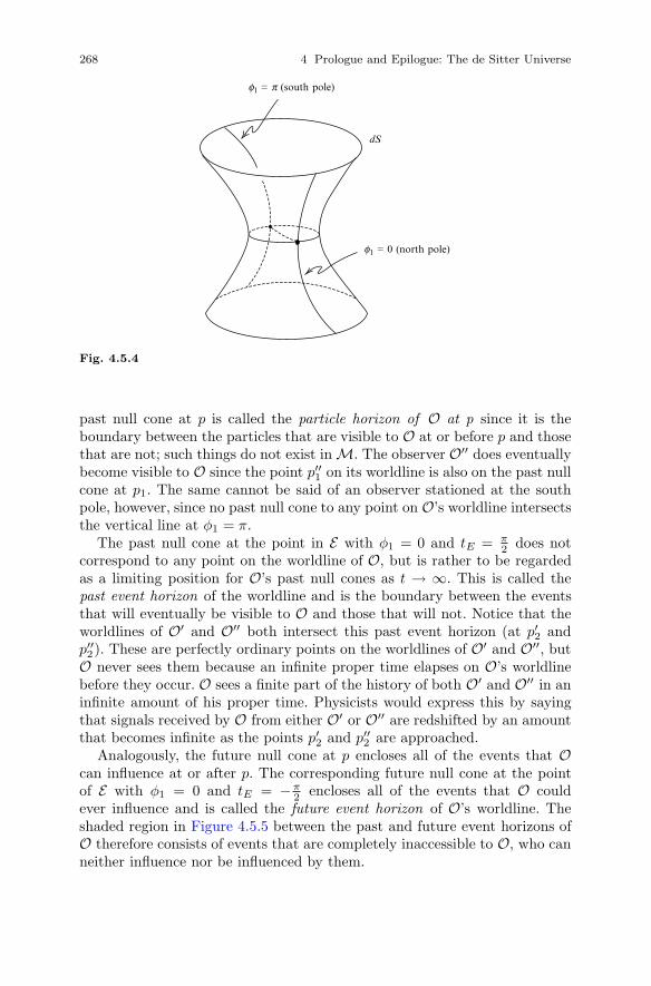
268 4 Prologue and Epilogue: The de Sitter Universe
dS
f1 = p (south pole)
f1 = 0 (north pole)
Fig. 4.5.4
past null cone at p is called the particle horizon of O at p since it is theboundary between the particles that are visible to O at or before p and thosethat are not; such things do not exist in M. The observer O′′ does eventuallybecome visible to O since the point p′′1 on its worldline is also on the past nullcone at p1. The same cannot be said of an observer stationed at the southpole, however, since no past null cone to any point on O’s worldline intersectsthe vertical line at φ1 = π.
The past null cone at the point in E with φ1 = 0 and tE = π2 does not
correspond to any point on the worldline of O, but is rather to be regardedas a limiting position for O’s past null cones as t → ∞. This is called thepast event horizon of the worldline and is the boundary between the eventsthat will eventually be visible to O and those that will not. Notice that theworldlines of O′ and O′′ both intersect this past event horizon (at p′2 andp′′2). These are perfectly ordinary points on the worldlines of O′ and O′′, butO never sees them because an infinite proper time elapses on O’s worldlinebefore they occur. O sees a finite part of the history of both O′ and O′′ in aninfinite amount of his proper time. Physicists would express this by sayingthat signals received by O from either O′ or O′′ are redshifted by an amountthat becomes infinite as the points p′2 and p′′2 are approached.
Analogously, the future null cone at p encloses all of the events that Ocan influence at or after p. The corresponding future null cone at the pointof E with φ1 = 0 and tE = −π
2encloses all of the events that O could
ever influence and is called the future event horizon of O’s worldline. Theshaded region in Figure 4.5.5 between the past and future event horizons ofO therefore consists of events that are completely inaccessible to O, who canneither influence nor be influenced by them.
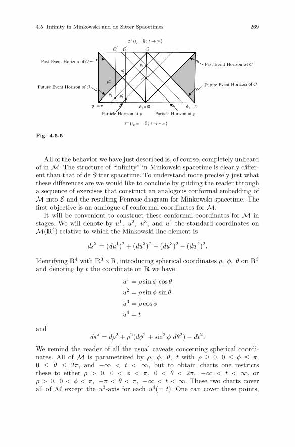
4.5 Infinity in Minkowski and de Sitter Spacetimes 269
f1 = 0f1 = π
Particle Horizon at p Particle Horizon at p
Past Event Horizon of
Future Event Horizon of
Past Event Horizon of
Future Event Horizon of
p
p1
p2
p1 p1
p2
f1 = π
+ (tE = π ; t → ∞ )2−
− (tE = − π ; t → −∞ )2−
" '
"
" '
'
Fig. 4.5.5
All of the behavior we have just described is, of course, completely unheardof in M. The structure of “infinity” in Minkowski spacetime is clearly differ-ent than that of de Sitter spacetime. To understand more precisely just whatthese differences are we would like to conclude by guiding the reader througha sequence of exercises that construct an analogous conformal embedding ofM into E and the resulting Penrose diagram for Minkowski spacetime. Thefirst objective is an analogue of conformal coordinates for M.
It will be convenient to construct these conformal coordinates for M instages. We will denote by u1, u2, u3, and u4 the standard coordinates onM(R4) relative to which the Minkowski line element is
ds2 = (du1)2 + (du2)2 + (du3)2 − (du4)2.
Identifying R4 with R3 ×R, introducing spherical coordinates ρ, φ, θ on R3
and denoting by t the coordinate on R we have
u1 = ρ sinφ cos θ
u2 = ρ sinφ sin θ
u3 = ρ cosφ
u4 = t
andds2 = dρ2 + ρ2(dφ2 + sin2 φ dθ2) − dt2.
We remind the reader of all the usual caveats concerning spherical coordi-nates. All of M is parametrized by ρ, φ, θ, t with ρ ≥ 0, 0 ≤ φ ≤ π,0 ≤ θ ≤ 2π, and −∞ < t < ∞, but to obtain charts one restrictsthese to either ρ > 0, 0 < φ < π, 0 < θ < 2π, −∞ < t < ∞, orρ > 0, 0 < φ < π, −π < θ < π, −∞ < t < ∞. These two charts coverall of M except the u3-axis for each u4(= t). One can cover these points,

270 4 Prologue and Epilogue: The de Sitter Universe
except for ρ = 0, with analogous spherical coordinates with, say, φ measuredfrom the u1-axis and θ in the u2u3-plane. Finally, to cover the points withρ = 0, −∞ < t < ∞, i.e., the t-axis, one selects some other point as the“origin” for an entirely analogous spherical coordinate chart. As is custom-ary, we sweep all of these variants under the rug and use ρ, φ, θ, t for thecoordinates in any one of these charts.
Next we introduce what are called advanced and retarded null coordinatesv and w by letting v = t + ρ and w = t− ρ. In somewhat more detail, we let
ρ =12
(v − w)
φ = φ
θ = θ (4.5.14)
t =12
(v + w)
Exercise 4.5.6(a) Show that v, w, φ, θ parametrize all of M for −∞ < w ≤ v < ∞, 0 ≤
φ ≤ π and 0 ≤ θ ≤ 2π and that each point of M is contained in an openset on which v, w, φ, θ are the coordinates of a chart for M.
(b) Show that, if a and b are constants, then the set of points in M with v = ais the lower half of the null cone at (u1, u2, u3, u4) = (0, 0, 0, a) andw = b is the upper half of the null cone at (u1, u2, u3, u4) = (0, 0, 0, b).
(c) Show that the line element for M in these coordinates is
ds2 =14
(v − w)2(dφ2 + sin2 φ dθ2) − dv dw .
Exercise 4.5.6 (b) provides a nice geometrical and physical interpretation ofthe new coordinates v and w. One finds v and w geometrically at a point xin M by locating points on the u4-axis at which the lower and upper nullcones intersect at x. Physically, one can express this in the following way.For v(x) one finds a spherical electromagnetic wave that is “incoming” tothe origin and experiences x, while for w(x) one finds such a wave that is“outgoing” from the origin. Then v(x) is the time t at which the incomingwave reaches the origin and w(x) is the time t at which the outgoing waveleft the origin. Succinctly, one connects x to the origin with light rays anduses the departure and arrival times as coordinates. Thus, v(x) (respectively,w(x)) is an advanced (respectively, retarded) null coordinate. Suppressing φand θ we can picture this in the ρt-plane as in Figure 4.5.6.
Next we once again use the arctangent function to “make infinity finite”,as Penrose and Rindler [PR2] put it. Specifically, we replace v and w by twonew coordinates p and q defined by p = arctan v and q = arctanw. In moredetail, we define
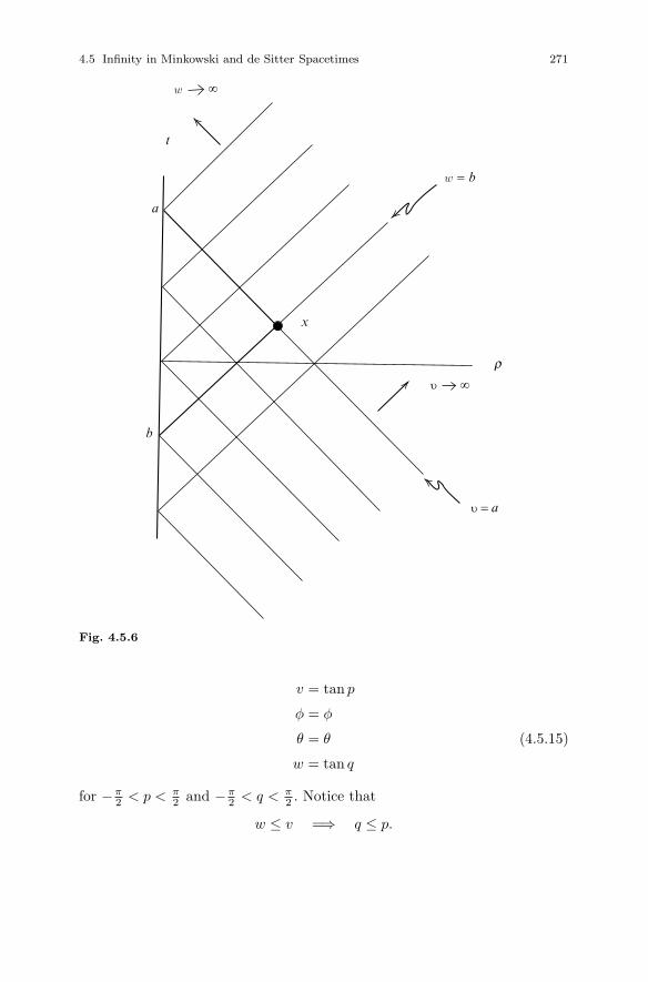
4.5 Infinity in Minkowski and de Sitter Spacetimes 271
∞
∞
w
w = b
t
υ
υ = a
a
b
r
x
Fig. 4.5.6
v = tan p
φ = φ
θ = θ (4.5.15)
w = tan q
for −π2 < p < π
2 and −π2 < q < π
2 . Notice that
w ≤ v =⇒ q ≤ p.
272 4 Prologue and Epilogue: The de Sitter Universe
Exercise 4.5.7(a) Show that p, q, φ, θ parametrize all of M for −π
2< q ≤ p < π
2, 0 ≤ φ ≤ π
and 0 ≤ θ ≤ 2π and that each point of M is contained in an open set onwhich p, q, φ, θ are the coordinates of a chart for M.
(b) Show that the line element for M in these coordinates is
ds2 =14
sec2 p sec2 q(−4dp dq + sin2 (p − q)
(dφ2 + sin2 φ dθ2
)).
Now, one final maneuver to bring this last line element into a more familiarform. Specifically, we introduce two new coordinates t′ and ρ′ by t′ = p + qand ρ′ = p − q, i.e.,
p =12(t′ + ρ′)
φ = φ
θ = θ (4.5.16)
q =12(t′ − ρ′)
for −π < t′ < π and 0 ≤ ρ′ < π.
Exercise 4.5.8(a) Show that ρ′, φ, θ, t′ parametrize all of M for 0 ≤ ρ′ < π, 0 ≤ φ ≤
π, 0 ≤ θ ≤ 2π, −π < t′ < π, and that each point of M is contained inan open set on which ρ′, φ, θ, t′ are the coordinates of a chart for M.
(b) Show that
2t = tan(
12
(t′ + ρ′))
+ tan(
12
(t′ − ρ′))
2ρ = tan(
12
(t′ + ρ′))− tan
(12
(t′ − ρ′))
.
(c) Show that the line element for M in these coordinates is
ds2 =14
sec2
(12
(t′ + ρ′))
sec2
(12
(t′ − ρ′)) (
dρ′2 +
sin2 ρ′(dφ2 + sin2 φdθ2) − dt ′2). (4.5.17)
Now we find ourselves in a familiar position. Except for the names of thevariables, dρ′2 + sin2 ρ′(dφ2 + sin2 φdθ2) − dt ′2 has precisely the same formas the line element (4.5.2) of the Einstein static universe in its standardcoordinates and the line element for M relative to (ρ′, φ, θ, t′) is justa positive multiple of this. We now ask the reader to argue as we did inExample 4.5.1 and draw the same conclusion.

4.5 Infinity in Minkowski and de Sitter Spacetimes 273
Exercise 4.5.9 Define a mapping F of M into E by
φ1 = ρ′
φ2 = φ
θ = θ
tE = t′
for 0 ≤ ρ′ < π, 0 ≤ φ ≤ π, 0 ≤ θ ≤ 2π and −π < t′ < π. Show that F is aconformal embedding of M into the region S3 × (−π, π) in E with
F ∗gE = Ω2gM,
where gM is the Lorentz metric on M and
Ω(ρ′, t′) = 2 cos(
12
(t′ + ρ′))
cos(
12
(t′ − ρ′))
. (4.5.18)
The image of the conformal embedding of dS into E was all ofS3 ×
(−π
2, π
2
), but it is not the case that the map F in Exercise 4.5.9 maps
onto S3 × (−π, π). To find the image we first find its boundary (which willeventually play the role of “infinity” in M)). As before we will construct ourpicture on the 2-dimensional cylinder by holding φ and θ fixed.
The “finite part” of M corresponds to −π2 < q ≤ p < π
2 so −π < t′ + ρ′ <π, −π < t′ − ρ′ < π, and 0 ≤ ρ′ ≤ π. Since φ1 = ρ′ and tE = t′, thesetranslate to −π < tE + φ1 < π, −π < tE − φ1 < π, and 0 ≤ φ1 < π. Thus,the boundary of the image of M in E is determined by tE + φ1 = ±π andtE − φ1 = ±π, subject to 0 ≤ φ1 ≤ π and −π ≤ tE ≤ π. Observe first that
tE + φ1 = −π, tE ≥ −π, and φ1 ≥ 0 =⇒ (tE , φ1) = (−π, 0)
and
tE − φ1 = π, tE ≤ π, and φ1 ≥ 0 =⇒ (tE , φ1) = (π, 0)
These two points in our picture we will denote
i− : tE + φ1 = −π(p = −π
2, q = −π
2
)and
i+ : tE − φ1 = π(p =
π
2, q =
π
2
)and, for reasons to be explained shortly, call them, respectively, past andfuture timelike infinity of M, while those satisfying
tE − φ1 = −π
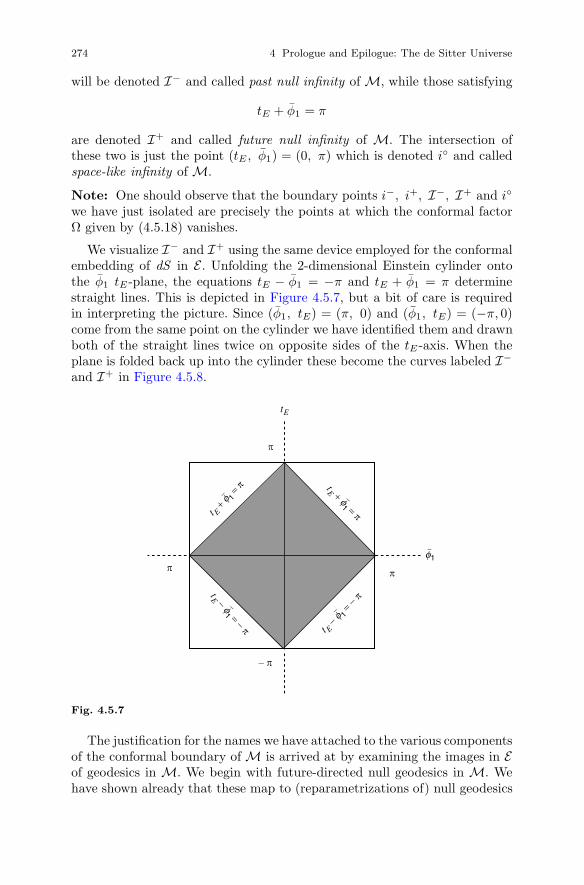
274 4 Prologue and Epilogue: The de Sitter Universe
will be denoted I− and called past null infinity of M, while those satisfying
tE + φ1 = π
are denoted I+ and called future null infinity of M. The intersection ofthese two is just the point (tE , φ1) = (0, π) which is denoted i◦ and calledspace-like infinity of M.
Note: One should observe that the boundary points i−, i+, I−, I+ and i◦
we have just isolated are precisely the points at which the conformal factorΩ given by (4.5.18) vanishes.
We visualize I− and I+ using the same device employed for the conformalembedding of dS in E . Unfolding the 2-dimensional Einstein cylinder ontothe φ1 tE-plane, the equations tE − φ1 = −π and tE + φ1 = π determinestraight lines. This is depicted in Figure 4.5.7, but a bit of care is requiredin interpreting the picture. Since (φ1, tE) = (π, 0) and (φ1, tE) = (−π, 0)come from the same point on the cylinder we have identified them and drawnboth of the straight lines twice on opposite sides of the tE -axis. When theplane is folded back up into the cylinder these become the curves labeled I−
and I+ in Figure 4.5.8.
− π
π π
π
t E + f 1
= π
−
tE + f1 = π
−
t E − f 1
= − π
−
tE − f1 = − π
−
tE
f1−
Fig. 4.5.7
The justification for the names we have attached to the various componentsof the conformal boundary of M is arrived at by examining the images in Eof geodesics in M. We begin with future-directed null geodesics in M. Wehave shown already that these map to (reparametrizations of) null geodesics
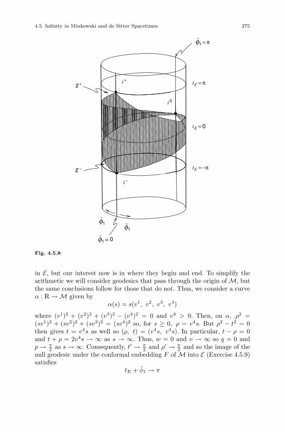
4.5 Infinity in Minkowski and de Sitter Spacetimes 275
f1
−
f1−
f1 = π−
f1 = 0−
tE = −π
tE = π
tE = 0
+ i +
i 0
I −
i −
i 0
I
Fig. 4.5.8
in E , but our interest now is in where they begin and end. To simplify thearithmetic we will consider geodesics that pass through the origin of M, butthe same conclusions follow for those that do not. Thus, we consider a curveα : R → M given by
α(s) = s(v1, v2, v3, v4)
where (v1)2 + (v2)2 + (v3)2 − (v4)2 = 0 and v4 > 0. Then, on α, ρ2 =(sv1)2 + (sv2)2 + (sv3)2 = (sv4)2 so, for s ≥ 0, ρ = v4s. But ρ2 − t2 = 0then gives t = v4s as well so (ρ, t) = (v4s, v4s). In particular, t − ρ = 0and t + ρ = 2v4s → ∞ as s → ∞. Thus, w = 0 and v → ∞ so q = 0 andp → π
2as s → ∞. Consequently, t′ → π
2and ρ′ → π
2and so the image of the
null geodesic under the conformal embedding F of M into E (Exercise 4.5.9)satisfies
tE + φ1 → π

276 4 Prologue and Epilogue: The de Sitter Universe
and so approaches I+. In the same way the image of α approaches I− ass → −∞. Although I− and I+ do not lie in M one thinks of future-directednull geodesics as beginning on I− and ending on I+.
A future-directed timelike geodesic through the origin in M is a curveα : R → M that can be written in the form
α(s) = s(v1, v2, v3, v4)
where (v1)2+(v2)2+(v3)2−(v4)2 = −1 and v4 > 0. The image of α under theconformal embedding of M into E need not be a geodesic, but it is a timelikecurve which we now ask the reader to show must begin on i− and i+.
Exercise 4.5.10 Show that the image in E of the future-directed timelikegeodesic α approaches i− as s → ∞ and i+ as s → ∞.
A spacelike geodesic α :R → M in M can be written as α(s) =s(v1, v2, v3, v4), where (v1)2 +(v2)2 +(v3)2− (v4)2 = 1 and one can assumewithout loss of generality that v4 ≥ 0. The image of α under the conformalembedding of M into E need not be a geodesic, but it is a spacelike curve.
Exercise 4.5.11 Show that the image in E of the spacelike geodesic α ap-proaches i◦ as s → ∞ and also as s → −∞.
i 0i 0
i −
i +
I −I −
I + I +
Fig. 4.5.9
Figure 4.5.9 is just Figure 4.5.7 again with all of the various pieces of the con-formal boundary of M identified by name and images in E of a few geodesicsof each type in M included. This is the Penrose diagram of Minkowski space-time and, contrasted with the corresponding diagram for dS (Figure 4.5.5),it does much to elucidate the differences in causal structure between the two.There are, for example, no particle or event horizons in M precisely becausetimelike geodesics “focus” on i− and i+ rather than I− and I+ so that the
4.5 Infinity in Minkowski and de Sitter Spacetimes 277
null cone at any point “catches” all of the timelike worldlines. This techniquehas been used to great effect in general relativity, but it goes much furtherthan this. Penrose devised the technique to study the asymptotic behaviorof solutions to massless free-field equations in spinor form such as those withwhich we concluded Section 3.6. The behavior of interest is conformally in-variant and so, rather than employing complicated limiting procedures, onecan analyze the behavior at points of I− and I+ using the more familiarlocal techniques of geometry and analysis. This is quite another story, how-ever, and the best service we can provide for those interested in pursuing thematter is to send them from here to [Pen2].

Appendix A
Topologies For M
A.1 The Euclidean Topology
In this appendix we wish to lay before the reader certain material whichrequires a bit more in the way of background than the text itself and whichadmittedly has not had a profound impact on subsequent research in rela-tivity, but which is nonetheless remarkable from both the physical and themathematical points of view. We will assume a very basic familiarity withelementary point-set topology and adopt [Wi] as our canonical reference.
The subject we wish to address had its origins in the extraordinary paper[Z2] of Zeeman in 1967. Zeeman observed that the ordinary Euclidean topol-ogy for M (defined below) has, from the relativistic viewpoint, no physicalsignificance or justification and proposed an alternative he called the “fine”topology. This topology was easy to describe, physically well motivated andhad the remarkable property that its homeomorphism group (also definedbelow) was essentially just the Lorentz group (together with translations andnonzero scalar multiplications). Thus, perhaps the most important group inall of physics is seen to emerge at the very primitive level of topology, i.e.,from just an appropriate definition of “nearby” events. The fine topology is,however, from the technical point of view, rather difficult to work with andthe arguments in [Z2] are by no means simple. In 1976, Hawking, King andMcCarthy [HKM] described another topology on M which seemed physi-cally even more natural, had precisely the same homeomorphism group asZeeman’s fine topology and required for the proof of this nothing beyondthe most rudimentary point-set topology and Zeeman’s Theorem 1.6.2. Thisso-called “path topology” for M is the object of our investigations in thisappendix.
We begin by transferring to M the standard Euclidean topology ofR4 via alinear isomorphism. Specifically, we select some fixed admissible basis {ea}4
a=1
for M (this determines an obvious linear isomorphism of M onto R4). If x =xaea and x0 = xa
0ea are two points in M we define the E-distance from x0 to
, : An Introduction , Applied Mathematical Sciences 92,
G.L. Naber The Geometry of Minkowski Spacetime to the Mathematics of the Special Theory of RelativityDOI 10.1007/978-1-4419-7838-7, © Springer Science+Business Media, LLC 2012
279
280 A Topologies For M
x by dE(x0, x) =((
x1 − x10
)2 +(x2 − x2
0
)2 +(x3 − x3
0
)2 +(x4 − x4
0
)2)1/2
.Then dE is a metric on M, i.e., satisfies (1) dE(x, x0) = dE(x0, x), (2)dE(x0, x) ≥ 0 and dE(x0, x) = 0 if and only if x = x0, and (3) dE(x0, x) ≤dE(x0, y)+dE(y, x) for all x0, x and y in M. Consequently, dE determines, inthe usual way (3.2 of [Wi]) a topology E for M called the Euclidean (or E-)topology. Specifically, if x0 is in M and ε > 0 we define the E-open ball ofradius ε about x0 by
NEε (x0) = {x ∈ M : dE(x0, x) < ε}.
A subset V of M is then said to be E-open if for every x0 in V there existsan ε > 0 such that NE
ε (x0) ⊆ V . The collection of all E-open sets in M con-stitutes the E-topology for M. When thinking of M as being endowed withthe Euclidean topology we will denote it ME . E’s will likewise be appendedto various other terms and symbols to emphasize that we are operating in theEuclidean topology, e.g., maps will be referred to as “E-continuous”, “ClE A”and “bdyE A” will designate the E-closure and E-boundary of A and so on.ME is, of course, homeomorphic to R4 with its customary Euclidean topologyso that its basic topological properties are well-known,1 e.g., it is first count-able, separable, locally compact, but not compact, pathwise connected, etc.
Notice that the definition of the E-metric dE on M is not invariant underLorentz transformations. That is, if dE(x0, x) is computed by the definingformula from the coordinates of x0 and x relative to another admissible basis{ea} for M the result will, in general, be different. The reason for this is clearsince the two bases are related by an element of L and elements of L preservethe Lorentz inner product and not the Euclidean inner product (i.e., theysatisfy Λ−1 = ηΛT η rather than Λ−1 = ΛT ). Nevertheless, two such metrics,while not equal, are equivalent in the sense that they determine the sametopology for M (because an element of L is a one-to-one linear map of Monto M and so an E-homeomorphism).
A.2 E-Continuous Timelike Curves
In Section 1.4 we defined what it meant for a smooth curve in M to be“timelike” and “future- (or past-) directed”. For the definition of the topologywe propose to describe in the next section it is essential to extend thesenotions to the class of curves in M that are E-continuous, but need nothave a velocity vector at each point. Thus, we let I denote a (nondegenerate)interval in R (open, closed, or half-open) and consider a curve α : I → Mthat is E-continuous (i.e., α−1(V ) is open in I for every E-open set V in M).
1 Its not-so-basic topological properties are quite another matter, however. Indeed, in manytopological ways, R4 is unique among the Euclidean spaces Rn (see, for example, [FL]).

A.2 E-Continuous Timelike Curves 281
Fix a t0 in I. We say that α is future-timelike at t0 if there exists a connected,relatively open subset U of I containing t0 such that
t ∈ U and t < t0 =⇒ α(t) � α(t0)
andt ∈ U and t0 < t =⇒ α(t0) � α(t).
(U is an interval which may contain one or both of the endpoints of I, if Ihappens to have endpoints). Past-timelike at t0 is defined similarly. α is saidto be future-timelike (resp., past-timelike) if it is future-timelike (resp., past-timelike) at every t0 in I. Finally, α is timelike if it is either future-timelikeor past-timelike.
Any curve α : I → M that is smooth has component functions rel-ative to any admissible basis that are continuous as maps from I into R.Since ME is homeomorphic to R4 with its product topology, such an α isE-continuous (8.8 of [Wi]). According to Lemma 1.4.7, a smooth curve thatis timelike and future-directed in the sense of Section 1.4 is therefore alsofuture-timelike in our new sense. Of course, the same is true of smooth, time-like and past-directed curves. However, any timelike polygon (which has novelocity vector at its “joints”) can obviously be parametrized so as to becomeeither future-timelike or past-timelike, but is not “smooth-timelike”. Oddlyenough, an E-continuous curve can be timelike and smooth without beingsmooth-timelike in the sense of Section 1.4. For example, if {ea} is an ad-missible basis and if one defines α : R → M by α(t) = (sin t)e1 + te4, thenα is future-timelike and smooth, but α′(t) = (cos t)e1 + e4 which is null att = nπ, n = 0, ±1, ±2, . . . (see Figure A.2.1). This is unfortunate sinceit complicates the physical interpretation of “E-continuous future-timelike”somewhat. One would like to regard such a curve as the worldline of a mate-rial particle which may be undergoing abrupt changes in speed and direction(due, say, to collisions). Of course, having a null velocity vector at some pointwould tend to indicate a particle momentarily attaining the speed of light andthis we prefer not to admit as a realistic possibility. One would seem forcedto accept a curve of the type just described as an acceptable model for theworldline of a material particle only on the intervals between points at whichthe tangent is null (notice that the situation cannot get much worse, i.e.,the velocity vector of a smooth future-timelike curve cannot be null on aninterval, nor can it ever be spacelike).
We proceed now to derive a sequence of results that will be needed in thenext section.
Lemma A.2.1 Let {ea}4a=1 be an admissible basis for M and α : I →
M an E-continuous timelike curve. If α is future-timelike, then x4(α(t)) isincreasing on I. If α is past-timelike, then x4(α(t)) is decreasing on I. Inparticular, if α is timelike, it is one-to-one.

282 A Topologies For M
Fig. A.2.1
Proof: Suppose α is future-timelike (the argument for α past-timelike issimilar). Let t0, t1 ∈ I with t0 < t1. We show that x4(α(t0)) < x4(α(t1)).Suppose, to the contrary, that x4(α(t0)) ≥ x4(α(t1)). x4(α(t)) is a real-valuedcontinuous (8.8 of [Wi]) function on the closed bounded interval [t0, t1] andso achieves a maximum value at some t2 ∈ [t0, t1]. Since α is future-timelikeat t0 and p � q implies x4(p) < x4(q), x4(α(t)) must increase immediatelyto the right of t0 so t2 > t0. But x4(α(t2)) > x4(α(t0)) ≥ x4(α(t1)) impliest2 < t1 so t2 ∈ (t0, t1). But α is future-timelike at t2 and so x4(α(t)) mustincrease immediately to the right of t2 and this contradicts the fact that, on[t0, t1], x4(α(t)) has a maximum at t2. �
Next we show that Theorem 1.4.6 remains true if “smooth future-directedtimelike” is replaced with “E-continuous future-timelike”.
Theorem A.2.2 Let p and q be two points in M. Then p � q if and onlyif there exists an E-continuous future-timelike curve α : [a, b] → M such thatα(a) = p and α(b) = q.
Proof: The necessity is clear from Theorem 1.4.6. For the sufficiency weassume α : [a, b] → M is E-continuous future-timelike with α(a) = p andα(b) = q. For each t in [a, b] we select a connected, relatively open subsetUt of [a, b] containing t as in the definition of future-timelike at t. Then{Ut : t ∈ [a, b]} is an open cover of [a, b] so, by compactness (17.9 of [Wi]),we may select a finite subcover U = {Ua, Ut1 , . . . , Utn}.

A.2 E-Continuous Timelike Curves 283
By definition, a ∈ Ua. Moreover, if b ∈ Ua, then α(a) � α(b) and we aredone. If b /∈ Ua, then the right-hand endpoint s0 of Ua is less than or equalto b and not in Ua.
Select a Uti in U such that s0 ∈ Uti . Then Uti �= Ua, but Ua ∩ Uti �= ∅.Select a T0 ∈ Ua ∩ Uti such that a < T0 < ti. Now, if b ∈ Uti , then α(a) �α(T0) � α(ti) � α(b) and we are done. Otherwise, the right-hand endpoints1 of Uti is less than b and not in Uti . Repeat the process, beginning at T0
rather than a. Select a Utj in U with s1 ∈ Utj . Observe that Utj �= Ua andUtj �= Uti since s1 is in neither Ua nor Uti . However, Uti ∩Utj �= ∅. Select T1
as above and continue to repeat the process. Since U is finite and covers [a, b]the procedure must terminate in a finite number of steps with α(a) � α(b)as required. �
Next we prove that an E-continuous curve that is timelike at each pointin an interval must have the same causal character (future-timelike or past-timelike) at each point. In fact, we prove more.
Lemma A.2.3 Let α : I → M be an E-continuous curve. If α is timelikeat each t0 in the interior Int I of I, then α is timelike.
Proof: We first show that α is either future-timelike at each t0 ∈ Int I orpast-timelike at each t0 ∈ Int I. The procedure will be to show that the setS = {t0 ∈ Int I : α is future-timelike at t0} is both open and closed in IntI and so, since Int I is connected, is either ∅ or all of Int I (26.1 of [Wi]).Suppose then that S �= ∅. Let t0 ∈ S and select some U ⊆ Int I as in thedefinition of “future-timelike at t0”. We show that α is future-timelike ateach t in U so t0 ∈ U ⊆ S and, since t0 ∈ S was arbitrary, conclude that Sis open. First suppose there were a t1 > t0 in U at which α is past-timelike.
Exercise A.2.1 Relative to an admissible basis consider x4(α(t)) on [t0, t1]and argue as in the proof of Lemma A.2.1 to derive a contradiction.A similar argument shows that there can be no t1 < t0 in U at which α ispast-timelike. Thus, U ⊆ S as required so S is open. The same argumentshows that {t0 ∈ Int I : α is past-timelike at t0}, which is the complement ofS in Int I, is open in Int I so S is open and closed in Int I as required. Thus,either S = ∅ or S = Int I so α is either past-timelike at every t0 ∈ Int I orfuture-timelike at every t0 ∈ Int I.
Now we show that if I has endpoints then α must be timelike and have thesame causal character at these points that it has on Int I. The arguments are
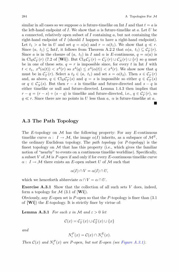
284 A Topologies For M
similar in all cases so we suppose α is future-timelike on Int I and that t = a isthe left-hand endpoint of I. We show that α is future-timelike at a. Let U bea connected, relatively open subset of I containing a, but not containing theright-hand endpoint of I (should I happen to have a right-hand endpoint).Let t1 > a be in U and set q = α(a) and r = α(t1). We show that q � r.Since (a, t1) ⊆ IntI, it follows from Theorem A.2.2 that α(a, t1) ⊆ C−
T (r).Since a is in the closure of (a, t1) in I and α is E-continuous, q = α(a) isin ClEC−
T (r) (7.2 of [Wi]). But ClEC−T (r) = C−
T (r) ∪ C−N (r) ∪ {r} so q must
be in one of these sets. q = r is impossible since, for every t in Int I witht < t1, x4(α(t)) < x4(r) so x4(q) ≤ x4(α(t)) < x4(r). We show now that qmust be in C−
T (r). Select a t2 ∈ (a, t1) and set s = α(t2). Then s ∈ C−T (r)
and, as above, q ∈ ClEC−T (s) and q = s is impossible so either q ∈ C−
T (s)or q ∈ C−
N (s). But then r − s is timelike and future-directed and s − q iseither timelike or null and future-directed. Lemma 1.4.3 then implies thatr − q = (r − s) + (s − q) is timelike and future-directed, i.e., q ∈ C−
T (r), soq � r. Since there are no points in U less than a, α is future-timelike at a.
�
A.3 The Path Topology
The E-topology on M has the following property: For any E-continuoustimelike curve α : I → M, the image α(I) inherits, as a subspace of ME ,the ordinary Euclidean topology. The path topology (or P-topology) is thefinest topology on M that has this property (i.e., which gives the familiarnotion of “nearby” to events on a continuous timelike worldline). Specifically,a subset V of M is P-open if and only if for every E-continuous timelike curveα : I → M there exists an E-open subset U of M such that
α(I) ∩ V = α(I) ∩ U,
which we henceforth abbreviate α ∩ V = α ∩ U .
Exercise A.3.1 Show that the collection of all such sets V does, indeed,form a topology for M (3.1 of [Wi]).Obviously, any E-open set is P -open so that the P -topology is finer than (3.1of [Wi]) the E-topology. It is strictly finer by virtue of:
Lemma A.3.1 For each x in M and ε > 0 let
C(x) = C−T (x) ∪ C+
T (x) ∪ {x}
andNP
ε (x) = C(x) ∩ NEε (x).
Then C(x) and NPε (x) are P-open, but not E-open (see Figure A.3.1).

A.3 The Path Topology 285
Fig. A.3.1
Proof: Neither set contains an NEδ (x) so they both fail to be E-open. Now,
let α : I → M be an E-continuous timelike curve. If α goes through x, thenα(I) is entirely contained in C(x) by Theorem A.2.2 so α ∩ C(x) = α ∩M.If α does not go through x, then α ∩ C(x) = α ∩
(C−
T (x) ∪ C+T (x)). In either
case α ∩ C(x) = α ∩ U for some E-open set U in M so C(x) is P -open. Butthen NP
ε (x) is the intersection of two P -open sets and so is P -open. �
M endowed with the P -topology is denoted MP and we now show that thesets NP
ε (x) form a base (5.1 of [Wi]) for MP .
Theorem A.3.2 The sets NPε (x) for x ∈ M and ε > 0 form a base for the
open sets in MP .
Proof: Let V ⊆ M be P -open and x ∈ V . We must show that there existsan ε > 0 such that NP
ε (x) ⊆ V . We assume that no such ε exists and producean E-continuous timelike curve α such that α∩V cannot be written as α∩Ufor any E-open set U and this is, of course, a contradiction.
We begin with NP1 (x) which, by assumption, is not contained in V . Since
no NPε (x) is contained in V one or the other of C+
T (x) ∩ NP1 (x) or C−
T (x) ∩NP
1 (x) (or both) must contain an infinite sequence {x1, x2, . . .} of points notin V which E-converges to x. Since the proof is the same in both cases weassume that this sequence is in C+
T (x) ∩ NP1 (x). We select a subsequence
{xni}∞i=0 as follows: Let xn0 = x1. Since x ∈ C−T (xn0 ) we may select a δ1 > 0
such that NEδ1
(x) ⊆ C−T (xn0) (see Figure A.3.2). Let ε1 = min{δ1, 1/2}. Select
an xn1 in the sequence which lies in NPε1
(x). Then x � xn1 � xn0 . Repeatthe procedure. Since x ∈ C−
T (xn1) there exists a δ2 > 0 such that NEδ2
(x) ⊆C−
T (xn1). Let ε2 = min{δ2, 1/22} and select an xn2 in the sequence which lies

286 A Topologies For M
Fig. A.3.2
in NEε2
(x). Then x � xn2 � xn1 � xn0 . Continuing inductively we constructa subsequence {xn0 , xn1 , xn2 , . . .} of {xn} such that
x � · · · � xni � · · · � xn2 � xn1 � xn0
and {xni}∞i=0 E-converges to x. Now define α : (0, 1] → M as follows: On[12, 1], α is a linear parametrization of the future-timelike segment from
xn1 to xn0 . On[
13, 1
2
], α is a linear parametrization of the future-timelike
segment from xn2 to xn1 , and so on. Then α is obviously E-continuous andfuture-timelike. Since the xni E-converge to x we can define an E-continuouscurve α : [0, 1] → M by
α(t) ={
α(t), 0 < t ≤ 1x, t = 0;
α is also future-timelike by Lemma A.2.3.Now, suppose α∩V = α∩U for some E-open set U . Since the xni are not in
V, xni �∈α∩V for each i so xni �∈α∩U for each i. Thus, {xni} ⊆ M−(α∩U) =(M−α)∪ (M−U). But xni ∈ α so we must have xni ∈ M−U . But M−Uis E-closed and {xni} E-converges to x so x ∈ M − U , i.e., x �∈U . Thus,x �∈ α∩U = α∩V and this is a contradiction since x is in both α and V . �
A number of basic topological properties of MP follow immediately fromTheorem A.3.2. Since the NP
ε (x) with ε rational form a local base at x, MP isfirst countable (4.4(b) of [Wi]). Since P -open sets have nonempty E-interior,MP is separable (5F of [Wi]). If R is a light ray in M and x ∈ R, then

A.3 The Path Topology 287
any NPε (x) intersects R only at x so, as a subspace of MP , R is discrete
(4G of [Wi]). R is also P -closed since it is, in fact, E-closed and the P -topology is finer than the E-topology. Being separable and containing suchlarge closed discrete subspaces prevents MP from being normal (15.1 of [Wi])since the Tietze Extension Theorem (15.8 of [Wi]) would require that all thecontinuous real-valued functions on any closed subspace extend to MP , butan uncountable closed discrete subspace has too many. In fact, it followseasily from our next lemma that MP is not even regular (14.1 of [Wi]) andtherefore certainly not normal (although it is Hausdorff since any two distinctpoints are contained in disjoint basic open sets).
Lemma A.3.3 The closure in MP of NPε (x) is ClE
(NP
ε (x))− (bdyE(
NEε (x)
)∩ bdyE(C(x))
)(see Figure A.3.3).
Proof: Since P is finer than E, ClP (A) ⊆ ClE(A) for any subset Aof M. Moreover, the points in bdyE
(NE
ε (x))∩ bdyE(C(x)) are not in
ClP(NP
ε (x))
since, if y is such a point, NPε/2(y) does not intersect NP
ε (x)(the null cone at y is tangent to the surface of the Euclidean ball NE
ε (x)at such a y) (see Figure A.3.4.). Thus, ClP
(NP
ε (x))
⊆ ClE(NP
ε (x))−(
bdyE
(NE
ε (x))∩ bdyE(C(x))
). But the reverse containment is also clear
since, if y is in the set on the right-hand side, every NPδ (y) intersects NP
ε (x).�
From Lemma A.3.3 it is clear that MP is not regular since no NPε (x)
contains a ClP(NP
δ (x)). Moreover, since any P -compact set is necessarily
E-compact and no ClP(NP
ε (x))
is E-compact (or even E-closed) we findthat no point in MP has a compact neighborhood. In particular, MP is notlocally compact (18.1 of [Wi]).
Fig. A.3.3
Exercise A.3.2 Show that MP is not countably compact (17.1 of [Wi]),Lindelof (16.5 of [Wi]), or second countable (16.1 of [Wi]).
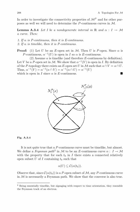
288 A Topologies For M
In order to investigate the connectivity properties of MP and for other pur-poses as well we will need to determine the P -continuous curves in M.
Lemma A.3.4 Let I be a nondegenerate interval in R and α : I → Ma curve. Then:
1. If α is P-continuous, then it is E-continuous.2. If α is timelike, then it is P-continuous.
Proof: (1) Let U be an E-open set in M. Then U is P -open. Since α isP -continuous, α−1(U) is open in I so α is E-continuous.
(2) Assume α is timelike (and therefore E-continuous by definition).Let V be a P -open set in M. We show that α−1(V ) is open in I. By definitionof the P -topology there exists an E-open set U in M such that α∩V = α∩U .Thus, α−1(V ) = α−1(α ∩ V ) = α−1(α ∩ U) = α−1(U)which is open in I since α is E-continuous. �
Fig. A.3.4
It is not quite true that a P -continuous curve must be timelike, but almost.We define a Feynman path2 in M to be an E-continuous curve α : I → Mwith the property that for each t0 in I there exists a connected relativelyopen subset U of I containing t0 such that
α(U) ⊆ C(α(t0)).
Observe that, since C(α(t0)) is a P -open subset of M, any P -continuous curvein M is necessarily a Feynman path. We show that the converse is also true.
2 Being essentially timelike, but zigzaging with respect to time orientation, they resemblethe Feynman track of an electron.

A.3 The Path Topology 289
Theorem A.3.5 A curve α : I → M is P-continuous if and only if it is aFeynman path.
Proof: All that remains is to prove that a Feynman path α : I → M isP -continuous. Fix a t0 ∈ I. We show that α is P -continuous at t0. For thislet NP
ε (α(t0)) be a basic P -neighborhood of α(t0). Now, α−1(NP
ε (α(t0)))
=α−1(NE
ε (α(t0)) ∩ C(α(t0)))
= α−1(NE
ε (α(t0)))∩ α−1(C(α(t0))). Since α is
a Feynman path there exists a connected, relatively open subset U1 of I con-taining t0 such that U1 is contained in α−1(C(α(t0))). Since α is E-continuousby definition, there exists a connected, relatively open subset U2 of I con-taining t0 such that U2 ⊆ α−1
(NE
ε (α(t0))). Thus, if U = U1 ∩ U2 we have
t0 ∈ U ⊆ α−1(NP
ε (α(t0)))
so α(U) ⊆ NPε (α(t0)) and α is P -continuous at t0.
�
Since any two points in NPε (x) can be joined by a Feynman path (in fact,
by a timelike segment or two such segments “joined” at x), MP is locallypathwise connected (27.4 of [Wi]). Moreover, since any straight line in Mcan be approximated by a Feynman path, MP is also pathwise connected(27.1 of [Wi]) and therefore connected (27.2 of [Wi]).
Our next objective is to show that a P -homeomorphism h : MP → MP
of MP onto itself carries timelike curves onto timelike curves, i.e., that α :I → M is timelike if and only if h ◦ α : I → M is timelike. We provethis by characterizing timelike curves entirely in terms of set-theoretic andP -topological notions that are obviously preserved by P -homeomorphisms.
Theorem A.3.6 A curve α : I → M is timelike if and only if the followingtwo conditions are satisfied:
1. α is P-continuous and one-to-one2. For every t0 in I there exists a connected, relatively open subset U of I
containing t0 and a P-open neighborhood V of α(t0) in M such that:
(a) α(U) ⊆ V(b) Whenever t0 is in the interior of I and a and b are in U and satisfy
a < t0 < b, then every P-continuous curve in V joining α(a) and α(b)passes through α(t0).
Proof: First assume α is timelike. Since the proofs are the same in thetwo cases we will assume that α is future-timelike. Then α is P -continuousby Lemma A.3.4(2) and one-to-one by Lemma A.2.1 so (1) is satisfied. Nowfix a t0 in I and select U ⊆ I as in the definition of future-timelike at t0.Let V = C(α(t0)). Then V is a P -open neighborhood of α(t0) with α(U) ⊆V so part (a) of (2) is satisfied. Next suppose t0 is in the interior of Uand let a and b be in U with a < t0 < b. Then α(a) ∈ C−
T (α(t0)) andα(b) ∈ C+
T (α(t0)). Suppose γ : [c, d] → M is a P -continuous curve in Vwith γ(c) = α(a) and γ(d) = α(b). By P -continuity, γ[c, d] is a connected
290 A Topologies For M
subspace of MP (26.3 of [Wi]). But if α(t0) were not in the image of γ, thenγ[c, d] =
[γ[c, d] ∩ C−
T (α(t0))]∪[γ[c, d] ∩ C+
T (α(t0))]
would be a disconnection(26.1 of [Wi]) of γ[c, d]. Thus, (b) of (2) is also satisfied.
Conversely, suppose α : I → M satisfies (1) and (2). Then α is E-continuous by Lemma A.3.4. We show that α is timelike at each t0 in theinterior of I and appeal to Lemma A.2.3. Let U and V be as in (2). Assumewithout loss of generality that V is a basic open neighborhood NP
ε (α(t0)).Let U− = {t ∈ U : t < t0} and U+ = {t ∈ U : t > t0}. Select a ∈ U− andb ∈ U+. Since α is one-to-one, α(a) �= α(t0) and α(b) �= α(t0) so α(a) andα(b) both lie in C−
T (α(t0)) ∪ C+T (α(t0)). Assuming that α(a) is in C−
T (α(t0))we show that α is future-timelike at t0 (if α(a) ∈ C+
T (α(t0)) the same proofshows that α is past-timelike at t0). If α(b) were also in C−
T (α(t0)) we couldconstruct a Feynman path from α(a) to α(b) that is contained entirely inNP
ε (α(t0)) ∩ C−T (α(t0)). But such a Feynman path would be a P -continuous
curve in V joining α(a) and α(b) which could not go through α(t0), thuscontradicting part (b) of (2). Thus, α(b) ∈ C+
T (α(t0)). We conclude thatα(U−) ∩ C−
T (α(t0)) �= ∅ and α(U+) ∩ C+T (α(t0)) �= ∅. Since α is one-to-one,
α(t0) /∈ α(U−) and α(t0) /∈ α(U+). But α is P -continuous so α(U−) andα(U+) are both connected subspaces of MP and so we must have α(U−) ⊆C−
T (α(t0)) and α(U+) ⊆ C+T (α(t0)), i.e., α is future-timelike at t0. �
Corollary A.3.7 If h : MP → MP is a P-homeomorphism of MP ontoitself, then a curve α : I → M is timelike if and only if h ◦ α : I → M istimelike.
Proof: Conditions (1) and (2) of Theorem A.3.6 are both obviously pre-served by P -homeomorphisms. �
Corollary A.3.8 If h : MP → MP is a P-homeomorphism of MP ontoitself, then h carries CT (x) bijectively onto CT (h(x)) for every x in M.
Exercise A.3.3 Prove Corollary A.3.8. �
We wish to show that a P -homeomorphism either preserves or reverses theorder �. First, the local version.
Lemma A.3.9 Let h : MP → MP be a P-homeomorphism and x a fixedpoint in M. Then either
1. h(C−
T (x))
= C−T (h(x)) and h
(C+
T (x))
= C+T (h(x)) or
2. h(C−
T (x))
= C+T (h(x)) and h
(C+
T (x))
= C−T (h(x)).
Proof: Suppose there exists a p in C+T (x) with h(p) ∈ C+
T (h(x)) (the argu-ment is analogous if there exists a p in C+
T (x) with h(p) ∈ C−T (h(x))).
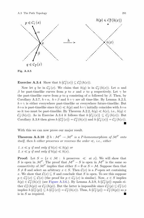
A.3 The Path Topology 291
Fig. A.3.5
Exercise A.3.4 Show that h(C+
T (x))⊆ C+
T (h(x)).
Now let q be in C−T (x). We claim that h(q) is in C−
T (h(x)). Let α andβ be past-timelike curves from p to x and x to q respectively. Let γ bethe past-timelike curve from p to q consisting of α followed by β. Then, byCorollary A.3.7, h ◦ α, h ◦ β and h ◦ γ are all time-like. By Lemma A.2.3,h ◦ γ is either everywhere past-timelike or everywhere future-timelike. Buth◦α is past-timelike since h(x) � h(p) and h◦γ initially coincides with h◦αso it too must be past-timelike. By Theorem A.2.2, h(q) � h(x), i.e., h(q) ∈C−
T (h(x)). As in Exercise A.3.4 it follows that h(C−
T (x))⊆ C−
T (h(x)). ButCorollary A.3.8 then gives h
(C+
T (x))
= C+T (h(x)) and h
(C−
T (x))
= C−T (h(x)).
�
With this we can now prove our major result.
Theorem A.3.10 If h : MP → MP is a P-homeomorphism of MP ontoitself, then h either preserves or reverses the order �, i.e., either
1. x � y if and only if h(x) � h(y) or2. x � y if and only if h(y) � h(x).
Proof: Let S = {x ∈ M : h preserves � at x}. We will show thatS is open in MP . The proof that MP − S is open in MP is the same soconnectivity of MP implies that either S = ∅ or S = M. Suppose then thatS �= ∅ and select an arbitrary x ∈ S. Then C(x) is a P -open set containingx. We show that C(x) ⊆ S and conclude that S is open. To see this supposep ∈ C+
T (x) ⊆ C(x) (the proof for p ∈ C−T (x) is similar). Now, x ∈ S implies
h(p) ∈ C+T (h(x)) (see Figure A.3.6.). By Lemma A.3.9, h
(C+
T (p))
equals ei-ther C+
T (h(p)) or C−T (h(p)). But the latter is impossible since C+
T (p) ⊆ C+T (x)
implies h(C+
T (p))⊆ h(C+
T (x))
= C+T (h(x)). Thus, h
(C+
T (p))
= C+T (h(p)) so p
is in S as required. �

292 A Topologies For M
Fig. A.3.6
From Theorem A.3.10 and Exercise 1.6.3 we conclude that if h : MP → MP
is a P -homeomorphism, then either h or −h is a causal automorphism.
Exercise A.3.5 Show that if h : M → M is a causal automorphism, thenh and −h are both P -homeomorphisms. Hint : Zeeman’s Theorem 1.6.2.Now, if X is an arbitrary topological space the set H(X) of all homeomor-phisms of X onto itself is called the homeomorphism group of X (it is closedunder the formation of compositions and inverses and so is indeed a groupunder the operation of composition). If G is a subset of H(X) we will saythat G generates H(X) if every homeomorphism of X onto itself can be writ-ten as a composition of elements of G. We now know that H(MP ) consistsprecisely of the maps ±h where h is a causal automorphism and Zeeman’sTheorem 1.6.2 describes all of these.
Theorem A.3.11 The homeomorphism group H(MP ) of MP is gener-ated by translations, dilations and (not necessarily orthochronous) orthogonaltransformations.
Modulo translations and nonzero scalar multiplications, H(MP ) is essentiallyjust the Lorentz group L.

Appendix B
Spinorial Objects
B.1 Introduction
Here we wish to examine in some detail the mathematical origin and physicalsignificance of the “essential 2-valuedness” of spinors, to which we alludedin Section 3.5. A genuine understanding of this phenomenon depends ontopological considerations of a somewhat less elementary nature than thoseinvolved in Appendix A. Thus, in Section B.3, we must assume a familiaritywith point-set topology through the construction of the fundamental groupand its calculation for the circle (see Sections 32–34 of [Wi] or Sections 1–4 of[G]). The few additional homotopy-theoretic results to which we must appealcan all be found in Sections 5–6 of [G].
As we left it in Chapter 3, Section 5, the situation was as follows: Eachnonzero spin vector ξA uniquely determines a future-directed null vector vand a 2-dimensional plane F spanned by v and a spacelike vector w or-thogonal to v. The pair (v, F) is called the null flag of ξA, with v theflagpole and F the flag. A phase change (rotation) ξA → eiθξA(θ ∈ R) ofthe spin vector ξA yields another spin vector with the same flagpole v asξA, but whose flag is rotated around this flag pole by 2θ relative to the flagof ξA. The crucial observation is that if ξA undergoes a continuous rotationξA → eiθξA, 0 ≤ θ ≤ π, through π, then the end result of the rotation is anew spin vector eiπξA = −ξA, but the same null flag. Let us reverse our pointof view. Regard the null flag (v,F) as a concrete geometrical representationof the spin vector ξA in much the same way that a “directed line segment”represents a vector in classical physics and Euclidean geometry. One thenfinds oneself in the awkward position of having to concede that rotating thisgeometrical object by 2π about some axis yields an object apparently indis-tinguishable from the first, but representing, not ξA, but −ξA. One mightseek additional geometrical data to append to the null flag (as we added theflag when we found that the flagpole itself did not uniquely determine ξA) inorder to distinguish the object representing ξA from that representing −ξA.
293

294 B Spinorial Objects
It is clear, however, that if “geometrical data” is to be understood in theusual sense, then any such data would also be returned to its original valueafter a rotation of 2π. The sign ambiguity in our geometrical representationof spin vectors seems unavoidable, i.e., “essential”. Perhaps even more curi-ous is the fact that a further rotation of the flag by 2π (i.e., a total rotationof 4π) corresponds to θ = 2π and so returns to us the original spin vectorξA = ei(2π)ξA and the original null flag.
This state of affairs is quite unlike anything encountered in classical physicsor geometry. By analogy, one would have to imagine a “vector” and its geo-metrical representation as a directed line segment with the property that, byrotating the arrow through 2π about some axis one obtained the geometri-cal representation of some other “vector”. But, of course, classical Euclideanvector (and, more generally, tensor) analysis is built on the premise that thiscannot be the case. Indeed, a vector (tensor) is just a carrier of some repre-sentation of the rotation group and the element of the rotation group corre-sponding to rotation by 2π about any axis is the identity. This is, of course,just a mathematical reflection of the conventional wisdom that rotating anisolated physical system through 2π yields a system that is indistinguishablefrom the first.
B.2 The Spinning Electron and Dirac’s Demonstration
“Conventional wisdom” has not fared well in modern physics so it may comeas no surprise to learn that there are, in fact, physical systems at the sub-atomic level whose state is altered by a rotation of the system through 2πabout some axis, but is returned to its orginal value by a rotation through4π. Indeed, any of the elementary particles in nature classified as a Fermions(electrons, protons, neutrons, neutrinos, etc.) possess what the physicists call“half-integer spin” and, as a consequence, their quantum mechanical descrip-tions (“wave functions”) behave in precisely this way (a beautifully lucid andelementary account of the physics involved here is available in Volume IIIof the Feynman Lectures on Physics [Fe]). That the spin state of an elec-tron behaves in this rather bizarre way has been known for many years, but,because of the way in which quantum mechanics decrees that physical infor-mation be extracted from an object’s wave function, was generally thoughtto have no observable consequences. More recently it has been argued that itis possible, in principle, to construct devices in which this behavior under ro-tation is exhibited on a macroscopic scale (see [[AS], [KO] and [M]). Theseconstructions, however, depend on a rather detailed understanding of howelectrons are described in quantum mechanics. Fortunately, Paul Dirac hasdevised a remarkably ingenious demonstration involving a perfectly mundanemacroscopic physical system in which “something” in the system’s state isaltered by rotation through 2π, but returned to its original value by a 4π
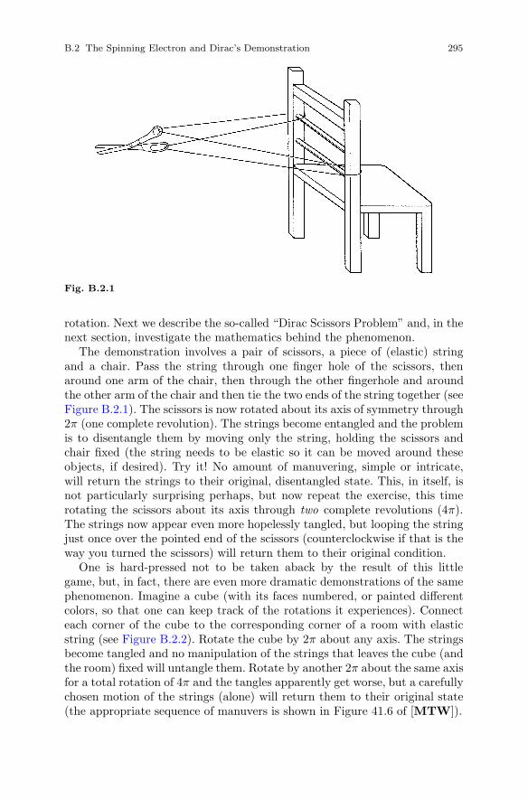
B.2 The Spinning Electron and Dirac’s Demonstration 295
Fig. B.2.1
rotation. Next we describe the so-called “Dirac Scissors Problem” and, in thenext section, investigate the mathematics behind the phenomenon.
The demonstration involves a pair of scissors, a piece of (elastic) stringand a chair. Pass the string through one finger hole of the scissors, thenaround one arm of the chair, then through the other fingerhole and aroundthe other arm of the chair and then tie the two ends of the string together (seeFigure B.2.1). The scissors is now rotated about its axis of symmetry through2π (one complete revolution). The strings become entangled and the problemis to disentangle them by moving only the string, holding the scissors andchair fixed (the string needs to be elastic so it can be moved around theseobjects, if desired). Try it! No amount of manuvering, simple or intricate,will return the strings to their original, disentangled state. This, in itself, isnot particularly surprising perhaps, but now repeat the exercise, this timerotating the scissors about its axis through two complete revolutions (4π).The strings now appear even more hopelessly tangled, but looping the stringjust once over the pointed end of the scissors (counterclockwise if that is theway you turned the scissors) will return them to their original condition.
One is hard-pressed not to be taken aback by the result of this littlegame, but, in fact, there are even more dramatic demonstrations of the samephenomenon. Imagine a cube (with its faces numbered, or painted differentcolors, so that one can keep track of the rotations it experiences). Connecteach corner of the cube to the corresponding corner of a room with elasticstring (see Figure B.2.2). Rotate the cube by 2π about any axis. The stringsbecome tangled and no manipulation of the strings that leaves the cube (andthe room) fixed will untangle them. Rotate by another 2π about the same axisfor a total rotation of 4π and the tangles apparently get worse, but a carefullychosen motion of the strings (alone) will return them to their original state(the appropriate sequence of manuvers is shown in Figure 41.6 of [MTW]).

296 B Spinorial Objects
Fig. B.2.2
In each of these situations there is clearly “something different” about thestate of the system when it has undergone a rotation of 2π and when it hasbeen rotated by 4π. Observe also that, in each case, the “system” is morethan just an isolated pair of scissors or a cube, but includes, in some sense,the way in which that object is “connected” to its surroundings. In the nextsection we return to mathematics to show how all of this can be said preciselyand, indeed, how the mathematics itself might have suggested the possibilityof such phenomena and the relevance of spinors to their description.
B.3 Homotopy in the Rotation and Lorentz Groups
We begin by establishing some notation and terminology and briefly review-ing some basic results related to the notion of “homotopy” in topology (agood, concise source for all of the material we will need is [G], Sections 1–6).Much of what we have to say will be true in an arbitrary topological space,but this much generality is not required and tends to obscure fundamentalissues with tiresome technicalities. For this reason we shall restrict our at-tention to the category of “connected topological manifolds”. A Hausdorfftopological space X is called an (n-dimensional) topological manifold if eachx ∈ X has an open neighborhood in X that is homeomorphic to an openset in Rn (18.3 of [Wi] or (6.8) of [G]). A path in X is a continuous mapα : [0, 1] → X . If α(0) = x0 and α(1) = x1, then α is a path from x0 to x1
in X and X is path connected if such a path exists for every pair of pointsx0, x1 ∈ X (27.1 of [Wi]).
Exercise B.3.1 Show that a topological manifold X that is connected (26.1of [Wi]) is necessarily path connected. Hint : Fix an arbitrary x0 ∈ X andshow that the set of all x1 ∈ X for which there is a path in X from x0 to x1
is both open and closed.

B.3 Homotopy in the Rotation and Lorentz Groups 297
Henceforth, “space” will mean “connected topological manifold”.Let α0 and α1 be two paths in X from x0 to x1. We say that α0 and α1
are (path) homotopic (with endpoints fixed) if there exists a continuous mapH : [0, 1] × [0, 1] → X , called a homotopy from α0 to α1, which satisfies
H(s, 0) = α0(s),H(s, 1) = α1(s),H(0, t) = x0,
H(1, t) = x1
for all s and t in [0, 1]. In this case we write α0 � α1. For each t in [0,1], αt(s) = H(s, t) defines a path in X from x0 to x1 and, intuitively, oneregards H as providing a “continuous deformation” of α0 into α1 through thefamily {αt : t ∈ [0, 1]} of paths. � is an equivalence relation on the set of allpaths from x0 to x1 and we denote the equivalence class of a path α by [α].The inverse of a path α from x0 to x1 is the path α−1 from x1 to x0 definedby α−1(s) = α(1 − s). One verifies that α0 � α1 implies α−1
0 � α−11 so one
may define the inverse of a homotopy equivalence class by [α]−1 = [α−1]. Ifα is a path from x0 to x1 in X and β is a path from x1 to x2 in X , then theproduct path βα from x0 to x2 is defined by
(βα)(s) =
{α(2s), 0 ≤ s ≤ 1
2
β(2s − 1), 12≤ s ≤ 1.
Again, α0 � α1 and β0 � β1 imply β0α0 � β1α1 so one may define theproduct of the homotopy equivalence classes [α] and [β] by [β][α] = [βα],provided the initial point of all the paths in [β] coincides with the terminalpoint of all the paths in [α]. A loop at x0 is a path from α(0) = x0 toα(1) = x0. Then α−1 is also a loop at x0. Moreover, if β is another loop atx0, then βα is defined and is also a loop at x0. Letting
π1(X, x0) = {[α] : α is a loop at x0},
one finds that the operations [α]−1 = [α−1] and [β][α] = [βα] give π1(X, x0)the structure of a group with identity element [x0], where we are here using x0
to designate also the constant (or trivial) loop at x0 defined by x0(s) = x0 forall s in [0, 1]. π1(X, x0) is called the fundamental group of X at x0. If x0 andx1 are any two points in X and γ is a path in X from x1 to x0 (guaranteed toexist by Exercise B.3.1), then [α] → [γ−1αγ] is an isomorphism of π1(X, x0)onto π1(X, x1). For this reason one generally writes π1(X) for any one of theisomorphic groups π1(X, x), x ∈ X , and calls π1(X) the fundamental groupof X. Obviously, homeomorphic spaces have the same (that is, isomorphic)fundamental groups. More generally, any two homotopically equivalent ((3.6)of [G]) spaces have the same fundamental groups.
298 B Spinorial Objects
A space is said to be simply connected if its fundamental group isisomorphic to the trivial group, i.e., if every loop is homotopic to the trivialloop (somewhat loosely one says that “every closed curve can be shrunk toa point”). Any Euclidean space Rn is simply connected ((3.2) of [G]), as isthe n-sphere Sn = {(x1, . . . , xn+1) ∈ Rn+1 : (x1)2 + · · · + (xn+1)2 = 1} forany n ≥ 2 (see Exercise B.3.5 and (4.13) of [G]). For n = 1, however, thesituation is different. Indeed, the fundamental group of the circle, π1(S1), isisomorphic to the additive group Z of integers ((4.4) of [G]). Essentially, aloop in S1 is characterized homotopically by the (integer) number of times itwraps around the circle (positive in one direction and negative in the other).
Exercise B.3.2 Let X and Y be two topological manifolds of dimensions nand m respectively. Show that X × Y , provided with the product topology,is a topological manifold of dimension n + m.
It is not difficult to show ((4.8) of [G]) that the fundamental group of aproduct X×Y is isomorphic to the direct product of the fundamental groupsof X and Y , i.e., π1(X×Y ) ∼= π1(X)×π1(Y ). In particular, the fundamentalgroup of the torus S1 × S1 is Z×Z.
In order to calculate several less elementary examples and, in the process,get to the heart of the connection between homotopy and spinorial objects,we require the notion of a “universal covering manifold”. As motivation letus consider again the circle S1. This time it is convenient to describe S1 asthe set of all complex numbers of modulus one, i.e., S1 = {z ∈ C : zz = 1}.Define a map p : R → S1 by p(θ) = e2πθi = cos(2πθ) + i sin(2πθ). Observethat p is continuous, carries 0 ∈ R onto 1 ∈ S1 and, in effect, “wraps” thereal line around the circle. Notice also that each z ∈ S1 has a neighborhoodU in S1 with the property that p−1(U) is a disjoint union of open sets in R,each of which is mapped homeomorphically by p onto U (this is illustratedfor z = 1 in Figure B.3.1). In particular, the “fiber” p−1(z) above each z ∈ S1
is discrete. Now let us consider a homeomorphism φ of R onto itself which“preserves the fibers of p”, i.e., satisfies p ◦φ = p, so that r ∈ p−1(z) impliesφ(r) ∈ p−1(z). We claim that such a homeomorphism is uniquely determinedby its value at 0 ∈ R (or at any other single point in R), i.e., that if φ1 and φ2
are two p-fiber preserving homeomorphisms of R onto R and φ1(0) = φ2(0),then φ1 = φ2. To see this let E = {e ∈ R : φ1(e) = φ2(e)}. Then E �= ∅since 0 ∈ E and, by continuity of φ1 and φ2, E is closed in R. Since R isconnected the proof will be complete if we can show that E is open. Thus,let e be a point in E so that φ1(e) = φ2(e) = r for some r ∈ R. Noticethat p(φ1(e)) = p(r) and p(φ1(e)) = p(e) imply that p(e) = p(r). Now selectopen neighborhoods Ve and Vr of e and r which p maps homeomorphicallyonto a neighborhood U of p(e) = p(r). Let V = Ve ∩ φ−1
1 (Vr) ∩ φ2−1(Vr).
Then V is an open neighborhood of e contained in Ve and with φ1(V ) ⊆ Vr
and φ2(V ) ⊆ Vr. For each v ∈ V , p(φ1(v)) = p(φ2(v)) since both equal p(v).But φ1(v), φ2(v) ∈ Vr and, on Vr, p is a homeomorphism so φ1(v) = φ2(v).Thus, V ⊆ E so E is open. We find then that the homeomorphisms of R that

B.3 Homotopy in the Rotation and Lorentz Groups 299
preserve the fibers of p are completely determined by their values at 0. Sincethe elements in a single fiber p−1(z) clearly differ by integers, the value of ap-fiber preserving homeomorphism of R at 0 is an integer.
Fig. B.3.1
Exercise B.3.3 For each integer n let φn : R → R be the translation of Rby n, i.e., φn(y) = y + n for each y ∈ R. Show that the set C of p-fiber pre-serving homeomorphisms of R is precisely {φn : n ∈ Z}. Observe, moreover,that φn◦φm = φn+m so, as a group under the operation of composition, C isisomorphic to the additive group Z of integers, i.e., to π1(S1).
Distilling the essential features out of this last example leads to the fol-lowing definitions and results. Let X be a connected topological manifold.A universal covering manifold for X consists of a pair (X, p), where X isa simply connected topological manifold and p : X → X is a continuoussurjection (called the covering map) with the property that every x ∈ X hasan open neighborhood U such that p−1(U) is a disjoint union of open sets inX, each of which is mapped homeomorphically onto U by p. Every connectedtopological manifold has a universal covering manifold (X, p) ((6.8) of [G])that is essentially unique in the sense that if (X ′, p′) is another, then thereexists a homeomorphism ψ of X ′ onto X such that p◦ψ = p′ ((6.4) of [G]). Ahomeomorphism φ of X onto itself that preserves the fibers of p, i.e., satisfiesp◦φ = p, is called a covering transformation and the collection C of all suchis a group under composition. Moreover, C is isomorphic to π1(X) ((5.8) of[G]). C is often easier to contend with than π1(X) and we will now use it tocompute the examples of real interest to us.
We shall construct these examples “backwards”, beginning with a space Xthat will eventually be the universal covering manifold of the desired example

300 B Spinorial Objects
X , which is defined as a quotient (9.1 of [Wi]) of X. First take X to be the2-sphere S2 = {(x1, x2, x3) ∈ R3 : (x1)2 + (x2)2 + (x3)2 = 1} with thetopology it inherits as a subspace of R3.
Exercise B.3.4 Show that S2 is a (Hausdorff, 2-dimensional, connected,compact) topological manifold. Hint : Show, for example, that, on the upperhemisphere {(x1, x2, x3) ∈ S2 : x3 > 0}, the projection map (x1, x2, x3) →(x1, x2) is a homeomorphism onto the unit disc (x1)2 + (x2)2 < 1.
Exercise B.3.5 Show that Sn is a (Hausdorff, n-dimensional, connected,compact) topological manifold for any n ≥ 1.
Now define an equivalence relation ∼ on S2 by identifying antipodal points,i.e., if y, z ∈ S2, then y ∼ z if and only if z = ±y. Let [y] denote theequivalence class of y, i.e., [y] = {y,−y}, and denote by RP 2 the set of allequivalence classes. Define p : S2 → RP 2 by p(y) = [y] for every y ∈ S2
and provide RP 2 with the quotient topology determined by p (i.e., U ⊆ RP 2
is open if and only if p−1(U) is open in S2). RP 2 is then called the realprojective plane.
Exercise B.3.6 Show that RP 2 is a (Hausdorff, 2-dimensional, connected,compact) topological manifold.
Now, since S2 is simply connected and p : S2 → RP 2 clearly satisfies thedefining condition for a covering map and since universal covering manifoldsare unique we conclude that
RP2 ∼= S2.
But then π1(RP 2) is isomorphic to the group of p-fiber preserving home-omorphisms φ : S2 → S2 of S2. We claim that this group contains pre-cisely two elements, namely, the identity map (φ0(y) = y for every y ∈ S2)and the antipodal map (φ1(y) = −y for every y ∈ S2). To see this ob-serve that the fibers of p are just pairs of antipodal points {y,−y} so sucha φ must, for each y ∈ S2, satisfy either φ(y) = y or φ(y) = −y and soS2 = {y ∈ S2 : φ(y) = y} ∪ {y ∈ S2 : φ(y) = −y}. Since both of these setsare obviously closed, connectivity of S2 implies that one is ∅ and the otheris S2 as required. Thus, π1(RP 2) has precisely two elements and so must beisomorphic to the group of integers mod 2, i.e.,
π1(RP 2) ∼= Z2.
It will be important to us momentarily to observe that there is another wayto construct RP 2. For this we carry out the identification of antipodal pointson S2 in two stages. First identify points on the lower hemisphere (x3 < 0)with their antipodes on the upper hemisphere (x3 > 0), leaving the equator(x3 = 0) fixed. At this point we have a copy of the closed upper hemisphere(x3 ≥ 0) which, by projecting into the x1x2-plane, is homeomorphic to the
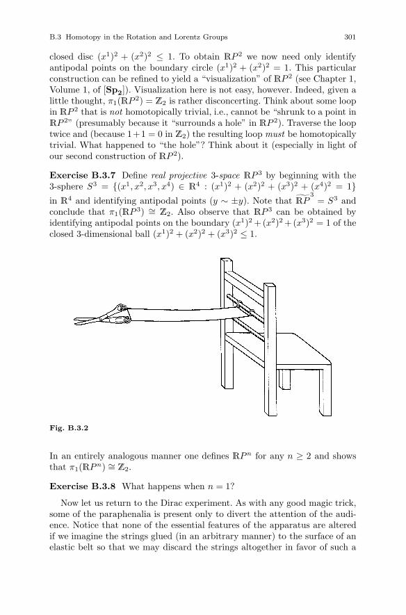
B.3 Homotopy in the Rotation and Lorentz Groups 301
closed disc (x1)2 + (x2)2 ≤ 1. To obtain RP 2 we now need only identifyantipodal points on the boundary circle (x1)2 + (x2)2 = 1. This particularconstruction can be refined to yield a “visualization” of RP 2 (see Chapter 1,Volume 1, of [Sp2]). Visualization here is not easy, however. Indeed, given alittle thought, π1(RP 2) = Z2 is rather disconcerting. Think about some loopin RP 2 that is not homotopically trivial, i.e., cannot be “shrunk to a point inRP 2” (presumably because it “surrounds a hole” in RP 2). Traverse the looptwice and (because 1+1 = 0 in Z2) the resulting loop must be homotopicallytrivial. What happened to “the hole”? Think about it (especially in light ofour second construction of RP 2).
Exercise B.3.7 Define real projective 3-space RP 3 by beginning with the3-sphere S3 = {(x1, x2, x3, x4) ∈ R4 : (x1)2 + (x2)2 + (x3)2 + (x4)2 = 1}in R4 and identifying antipodal points (y ∼ ±y). Note that RP
3= S3 and
conclude that π1(RP 3) ∼= Z2. Also observe that RP 3 can be obtained byidentifying antipodal points on the boundary (x1)2 +(x2)2 +(x3)2 = 1 of theclosed 3-dimensional ball (x1)2 + (x2)2 + (x3)2 ≤ 1.
Fig. B.3.2
In an entirely analogous manner one defines RPn for any n ≥ 2 and showsthat π1(RP n) ∼= Z2.
Exercise B.3.8 What happens when n = 1?
Now let us return to the Dirac experiment. As with any good magic trick,some of the paraphenalia is present only to divert the attention of the audi-ence. Notice that none of the essential features of the apparatus are alteredif we imagine the strings glued (in an arbitrary manner) to the surface of anelastic belt so that we may discard the strings altogether in favor of such a
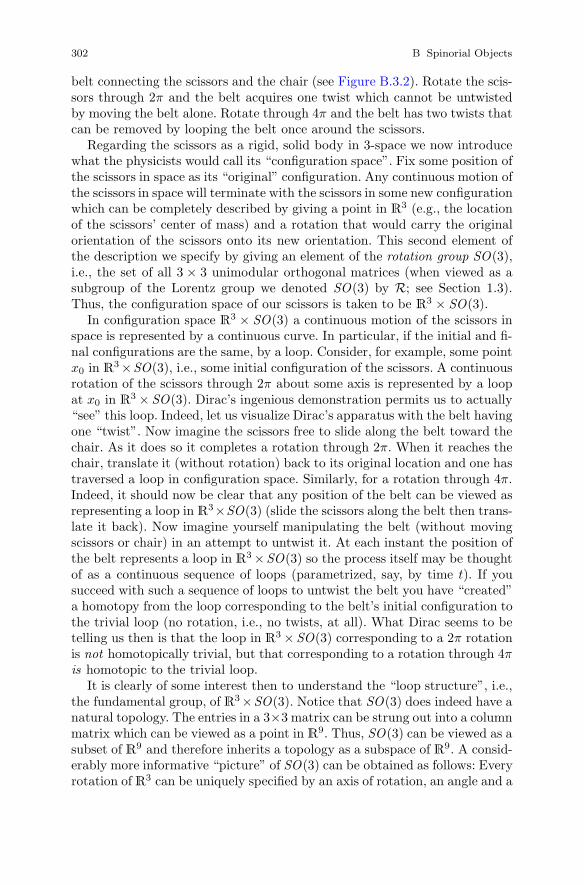
302 B Spinorial Objects
belt connecting the scissors and the chair (see Figure B.3.2). Rotate the scis-sors through 2π and the belt acquires one twist which cannot be untwistedby moving the belt alone. Rotate through 4π and the belt has two twists thatcan be removed by looping the belt once around the scissors.
Regarding the scissors as a rigid, solid body in 3-space we now introducewhat the physicists would call its “configuration space”. Fix some position ofthe scissors in space as its “original” configuration. Any continuous motion ofthe scissors in space will terminate with the scissors in some new configurationwhich can be completely described by giving a point in R3 (e.g., the locationof the scissors’ center of mass) and a rotation that would carry the originalorientation of the scissors onto its new orientation. This second element ofthe description we specify by giving an element of the rotation group SO(3),i.e., the set of all 3 × 3 unimodular orthogonal matrices (when viewed as asubgroup of the Lorentz group we denoted SO(3) by R; see Section 1.3).Thus, the configuration space of our scissors is taken to be R3 × SO(3).
In configuration space R3 × SO(3) a continuous motion of the scissors inspace is represented by a continuous curve. In particular, if the initial and fi-nal configurations are the same, by a loop. Consider, for example, some pointx0 in R3×SO(3), i.e., some initial configuration of the scissors. A continuousrotation of the scissors through 2π about some axis is represented by a loopat x0 in R3 × SO(3). Dirac’s ingenious demonstration permits us to actually“see” this loop. Indeed, let us visualize Dirac’s apparatus with the belt havingone “twist”. Now imagine the scissors free to slide along the belt toward thechair. As it does so it completes a rotation through 2π. When it reaches thechair, translate it (without rotation) back to its original location and one hastraversed a loop in configuration space. Similarly, for a rotation through 4π.Indeed, it should now be clear that any position of the belt can be viewed asrepresenting a loop in R3×SO(3) (slide the scissors along the belt then trans-late it back). Now imagine yourself manipulating the belt (without movingscissors or chair) in an attempt to untwist it. At each instant the position ofthe belt represents a loop in R3 ×SO(3) so the process itself may be thoughtof as a continuous sequence of loops (parametrized, say, by time t). If yousucceed with such a sequence of loops to untwist the belt you have “created”a homotopy from the loop corresponding to the belt’s initial configuration tothe trivial loop (no rotation, i.e., no twists, at all). What Dirac seems to betelling us then is that the loop in R3 × SO(3) corresponding to a 2π rotationis not homotopically trivial, but that corresponding to a rotation through 4πis homotopic to the trivial loop.
It is clearly of some interest then to understand the “loop structure”, i.e.,the fundamental group, of R3×SO(3). Notice that SO(3) does indeed have anatural topology. The entries in a 3×3 matrix can be strung out into a columnmatrix which can be viewed as a point in R9. Thus, SO(3) can be viewed as asubset of R9 and therefore inherits a topology as a subspace of R9. A consid-erably more informative “picture” of SO(3) can be obtained as follows: Everyrotation of R3 can be uniquely specified by an axis of rotation, an angle and a

B.3 Homotopy in the Rotation and Lorentz Groups 303
sense of rotation about the axis. We claim that all of this information can becodified in a single object, namely, a vector
⇀n in R3 of magnitude at most π.
Then the axis of rotation is the line along⇀n , the angle of rotation is |⇀n | and
the sense is determined by the “right-hand rule”. Notice that a rotation along⇀n through an angle θ with π ≤ θ ≤ 2π is equivalent to a rotation along –⇀n through 2π − θ so the restriction on |⇀n | is necessary (although not quitesufficient) to ensure that the correspondence between rotations and vectorsbe one-to-one. The set of vectors
⇀n in R3 with |⇀n | ≤ π is just the closed ball
of radius π about the origin. However, a rotation about⇀n through π is the
same as a rotation about –⇀n through π so antipodal points on the bound-
ary of this ball represent the same rotation and therefore must be identifiedin order that this correspondence with rotations be bijective. Carrying outthis identification yields, according to Exercise B.3.7, real projective 3-space(topologically, the radius of the ball is irrelevant, of course). One can write outanalytically the one-to-one correspondence we have just described geometri-cally to show that it is, in fact, continuous as a map from RP 3 to SO(3) ⊆ R9.Since RP 3 is compact (being a continuous image of S3), we find that SO(3)is homeomorphic to RP 3. In particular, π1(SO(3)) ∼= π1(RP 3) ∼= Z2. Thus,π1(R3 × SO(3)) ∼= π1(R3) × π1(SO(3)) ∼= {0} ×Z2 so
π1(R3 × SO(3)) ∼= Z2
and our suspicions are fully confirmed. In quite a remarkable way, the topol-ogy of the rotation group is reflected in the physical situation describedby Dirac.
Exercise B.3.9 In Z2, 1 + 1 + 1 = 1 and 1 + 1 + 1+ 1 = 0. More generally,2n + 1 = 1 and 2n = 0. What does this have to say about the scissorsexperiment?
But what has all of this to do with spinors? The connection is perhapsbest appreciated by way of a brief digression into semantics. We have calledR3 × SO(3) the “configuration space” of the object we have under consider-ation (the scissors). In the classical study of rigid body dynamics, however,it might equally well have been called its “state space” since, neglecting theobject’s (quite complicated) internal structure, it was (tacitly) assumed thatthe physical state of the object was entirely determined by its configurationin space. Suppressing the (topologically trivial and physically uninteresting)translational part of the configuration (i.e., R3), the body’s “state” was com-pletely specified by a point in SO(3). Based on our observations in Section 3.1,we would phrase this somewhat more precisely by saying that all of the phys-ically significant aspects of the object’s condition (as a rigid body) should bedescribable as carriers of some representation of SO(3) (keep in mind that,from our point of view, a rotated object is just the same object viewed froma rotated frame of reference). We shall refer to such quantities (which dependonly on the object’s configuration and not on “how it got there”) as tensorialobjects.

304 B Spinorial Objects
But the conclusion we draw from the Dirac experiment is that there maywell be more to a system’s “state” than merely its “configuration”. Thisadditional element has been called (see [MTW]) the version or orientation-entanglement relation of the system and its surroundings and at times it mustbe taken into account, e.g., when describing the quantum mechanical state ofan electron with spin. Where is one to look for a mathematical model for sucha system’s “state” if now there are two, where we thought there was one?The mathematics itself suggests an answer. Indeed, the universal coveringmanifold of SO(3) (i.e., of RP 3) is S3 and is, in fact, a double cover, i.e.,the covering map is precisely two-to-one, taking the same value at y and −yfor each y ∈ S3. Will S3 do as the “state space”? That this idea is not theshot-in-the-dark it may at first appear will become apparent once it has beenpointed out that we have actually seen all of this before.
Recall that, in Section 1.7, we constructed a homomorphism, called thespinor map, from SL(2,C) onto L that was also precisely two-to-one andcarried the unitary subgroup SU 2 of SL(2, C) onto the rotation subgroup R(i.e., SO(3)) of L.
Exercise B.3.10 Let I =[1 00 1
], i =
[i 00 −i
], j =
[0 1−1 0
]and k =
[0 ii 0
].
Show that I, i, j and k are all in SU 2 and that, moreover, any A ∈ SU 2 isuniquely expressible in the form
A = aI + bi + cj + dk,
where a, b, c, d ∈ R and a2 + b2 + c2 + d2 = 1. Regard SU 2 as a subset of R8
by identifying
A =
[a + bi c + di
−c + di a − bi
]with the column matrix col [a b c d − c d a − b] ∈ R8 and define a mapfrom SU 2 into R4 that carries this column matrix onto col [a b c d] ∈ R4.Show that this map is a homeomorphism of SU 2 onto S3 ⊆ R4. Finally,observe that the restriction of the spinor map to SU 2 is a continuous maponto R (i.e., SO(3)) which satisfies the defining property of a covering mapfor SO(3).
Thus we find that SU 2 and the restriction of the spinor map to it constitutea concrete realization of the universal covering manifold for SO(3) and itscovering map. Old friends, in new attire. And now, how natural it all appears.Identify a “state” of the system with some y ∈ SU 2. This corresponds to some“configuration” y ∈ SO(3) (the image of y under the spinor map). Rotatingthe system through 2π corresponds to a loop in SO(3) which, in turn, lifts((5.2) of [G]) to a path in SU 2 from y to −y (a different “state”). Furtherrotation of the system through 2π traverses the loop in SO(3) again, but,in SU 2, corresponds to a path from −y to y and so a rotation through 4πreturns the original “state”.
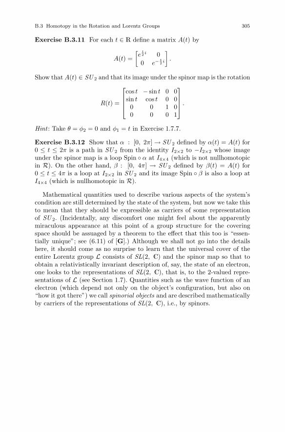
B.3 Homotopy in the Rotation and Lorentz Groups 305
Exercise B.3.11 For each t ∈ R define a matrix A(t) by
A(t) =[e
t2 i 00 e−
t2 i
].
Show that A(t) ∈ SU 2 and that its image under the spinor map is the rotation
R(t) =
⎡⎢⎢⎣cos t − sin t 0 0sin t cos t 0 00 0 1 00 0 0 1
⎤⎥⎥⎦ .
Hint : Take θ = φ2 = 0 and φ1 = t in Exercise 1.7.7.
Exercise B.3.12 Show that α : [0, 2π] → SU 2 defined by α(t) = A(t) for0 ≤ t ≤ 2π is a path in SU 2 from the identity I2×2 to −I2×2 whose imageunder the spinor map is a loop Spin ◦ α at I4×4 (which is not nullhomotopicin R). On the other hand, β : [0, 4π] → SU 2 defined by β(t) = A(t) for0 ≤ t ≤ 4π is a loop at I2×2 in SU 2 and its image Spin ◦ β is also a loop atI4×4 (which is nullhomotopic in R).
Mathematical quantities used to describe various aspects of the system’scondition are still determined by the state of the system, but now we take thisto mean that they should be expressible as carriers of some representationof SU 2. (Incidentally, any discomfort one might feel about the apparentlymiraculous appearance at this point of a group structure for the coveringspace should be assuaged by a theorem to the effect that this too is “essen-tially unique”; see (6.11) of [G].) Although we shall not go into the detailshere, it should come as no surprise to learn that the universal cover of theentire Lorentz group L consists of SL(2, C) and the spinor map so that toobtain a relativistically invariant description of, say, the state of an electron,one looks to the representations of SL(2, C), that is, to the 2-valued repre-sentations of L (see Section 1.7). Quantities such as the wave function of anelectron (which depend not only on the object’s configuration, but also on“how it got there”) we call spinorial objects and are described mathematicallyby carriers of the representations of SL(2, C), i.e., by spinors.


References
[AS] Aharonov, Y. and L. Susskind, “Observability of the sign change ofspinors under 2π rotations”, Phys. Rev., 158(1967), 1237–1238.
[A] Alphors, L., Complex Analysis, McGraw-Hill, New York, 1979.[BJ] Bade, W. L. and H. Jehle, “An introduction to spinors”, Rev. Mod.
Phys., 25(1953), 714–728.[B] Bolker, E. D., “The spinor spanner”, Amer. Math. Monthly,
80(1973), 977–984.[C] Cartan, E., The Theory of Spinors, M.I.T. Press, Cambridge,
MA, 1966.[CGK] Cacciatori, S., V. Girini and A. Kamenshchik, “Special relativity in
the 21st century”, Annalen der Physik, 17(2008), 728–768.[DS] Daigneault, A. and A. Sangalli, “Einstein’s static universe: an idea
whose time has come back”, Notices of AMS, 48(2001), 9–16.[E] Einstein, A., et al., The Principle of Relativity, Dover, New York,
1958.[Fa] Fadell, E., “Homotopy groups of configuration spaces and the string
problem of Dirac”, Duke Math. J., 29(1962), 231–242.[Fe] Feynman, R. P., R. B. Leighton and M. Sands, The Feynman Lec-
tures on Physics, Vol. III, Quantum Mechanics, Addison-Wesley,Reading, MA, 1966.
[FL] Freedman, M. H. and Feng Luo, Selected Applications of Geome-try to Low-Dimensional Topology, A.M.S. University Lecture Series,American Mathematical Society, Providence, RI, 1989.
[GMS] Gelfand, I. M., R. A. Minlos and Z. Ya. Shapiro, Representations ofthe Rotation and Lorentz Groups and their Applications, Pergamon,New York, 1963.
[G] Greenberg, M., Lectures on Algebraic Topology, W.A. Benjamin,New York, 1967.
[HE] Hawking, S.W. and G.F.R. Ellis, The Large Scale Structure ofSpace-Time, Cambridge University Press, Cambridge, England,1973.
307

308 References
[HKM] Hawking, S. W., A. R. King and P. J. McCarthy, “A new topologyfor curved spacetime which incorporates the causal, differential andconformal structures”, J. Math. Phys., 17(1976), 174–181.
[H] Herstein, I. N., Topics in Algebra, Blaisdell, Waltham, MA, 1964.[IS] Ives, H. E. and G. R. Stilwell, “Experimental study of the rate
of a moving atomic clock”, J. Opt. Soc. Am., 28(1938), 215;31(1941), 369.
[KO] Klein, A. G. and G. I. Opat, “Observability of 2π rotations: Aproposed experiment”, Phys. Rev. D, 11(1975), 523–528.
[K] Kuiper, N. H., Linear Algebra and Geometry, North Holland,Amsterdam, 1965.
[La] Lang, S., Linear Algebra, Springer-Verlag, New York, 1987.[LU] Laporte, O. and G. E. Uhlenbeck, “Application of spinor analysis
to the Maxwell and Dirac equations”, Phys. Rev., 37(1931), 1380–1397.
[LY] Lee, T. D. and C. N. Yang, “Parity nonconservation and a two-component theory of the neutrino”, Phys. Rev., 105(1957), 1671–1675.
[Le] Lenard, A., “A characterization of Lorentz transformations”, Amer.J. Phys., 19(1978), 157.
[Lest] Lester, J.A., “Separation-preserving transformations of de Sitterspacetime”, Abh. Math. Sem. Univ. Hamburg Volume 53, Number1, 217–224.
[M] Magnon, A. M. R., “Existence and observability of spinor struc-ture”, J. Math. Phys., 28(1987), 1364–1369.
[MTW] Misner, C. W., K. S. Thorne and J. A. Wheeler, Gravitation, W.H. Freeman, San Francisco, 1973.
[Nan] Nanda, S., “A geometrical proof that causality implies the Lorentzgroup”, Math. Proc. Camb. Phil. Soc., 79(1976), 533–536.
[N1] Naber, G. L., Topological Methods in Euclidean Spaces, Dover Pub-lications, Mineola, New York, 2000
[N2] Naber, G. L., Spacetime and Singularities, Cambridge UniversityPress, Cambridge, England, 1988.
[N3] Naber, G.L., Topology, Geometry and Gauge fields: Foundations,2nd Edition, Springer, New York, 2010.
[N4] Naber, G.L., Topology, Geometry and Gauge fields: Interactions,2nd Edition, Springer, New York, 2011.
[Ne] Newman, M. H. A., “On the string problem of Dirac”, J. LondonMath. Soc., 17(1942), 173–177.
[O’N] O’Neill, B., Semi-Riemannian Geometry, With Applications to Rel-ativity, Academic Press, San Diego, New York, 1983.
[Par] Parrott, S., Relativistic Electrodynamics and Differential Geometry,Springer-Verlag, New York, 1987.
[Pay] Payne, W. T., “Elementary spinor theory”, Amer. J. Phys.,20(1952), 253–262.

References 309
[Pen1] Penrose, R., “The apparent shape of a relativistically movingsphere”, Proc. Camb. Phil. Soc., 55(1959), 137–139.
[Pen2] Penrose, R., “Zero rest-mass fields including gravitation: asymptoticbehavior”, Proc. Roy. Soc. Lond., Series A, 284(1965), 159–203.
[PR] Penrose, R. and W. Rindler, Spinors and Spacetime, Vols. I–II,Cambridge University Press, Cambridge, England, 1984, 1986.
[R] Robb, A. A., Geometry of Space and Time, Cambridge UniversityPress, Cambridge, England, 1936.
[Sa] Salmon, G., A Treatise on the Analytic Geometry of Three Dimen-sions, Vol. 1, Chelsea, New York.
[Sp1] Spivak, M., Calculus on Manifolds, W.A. Benjamin, Inc., MenloPark, CA, 1965.
[Sp2] Spivak, M., A Comprehensive Introduction to Differential Geome-try, Vols. I–V, Publish or Perish, Houston, TX, 1975.
[Sy] Synge, J. L., Relativity: The Special Theory, North Holland,Amsterdam, 1972.
[TW] Taylor, E. F. and J. A. Wheeler, Spacetime Physics, W. H. Freeman,San Francisco, 1963.
[V] Veblen, O., “Spinors”, Science, 80(1934), 415–419.[Wald] Wald, R.M., General Relativity, University of Chicago Press,
Chicago, 1984.[We] Weyl, H., Space-Time-Matter, Dover, New York, 1952.[Wi] Willard, S., General Topology, Addison-Wesley, Reading, MA, 1970.[Z1] Zeeman, E. C., “Causality implies the Lorentz group”, J. Math.
Phys., 5(1964), 490–493.[Z2] Zeeman, E. C., “The topology of Minkowski space”, Topology,
6(1967), 161–170.


Symbols
M Minkowski spacetime, 9O, O, . . . observers, 2Σ, Σ, . . . spatial coordinate systems, 2c speed of light, 3S, S, . . . frames of reference, 3xa, xa, . . . spacetime coordinates, 3ΛT transpose of Λη 10g(v, w) = v · w value of the inner product g on (v, w), 7W⊥ orthogonal complement of W , 7Q quadratic form determined by g, 7v2 = Q(v) = v · v 7{ea}, {ea}, . . . orthonormal bases, 8δab = δab = δa
b = δab 4 × 4 Kronecker delta
ηab = ηab entries of η, 10CN (x0) null cone at x0, 11Rx0,x null worldline through x0 and x, 11Λ = [Λa
b] matrix of an orthogonal transformation, 13[Λa
b] inverse of [Λab]
LGH general homogeneous Lorentz group, 14CT (x0) time cone at x0, 16C±
T (x0) future and past time cones at x0, 16C±
N (x0) future and past null cones at x0, 17L Lorentz group, 19R rotation subgroup of L, 20⇀u,
⇀
u , . . . velocity 3-vectors, 21β relative speed of S and S, 21, 26γ (1 − β2)−
12 , 21
311
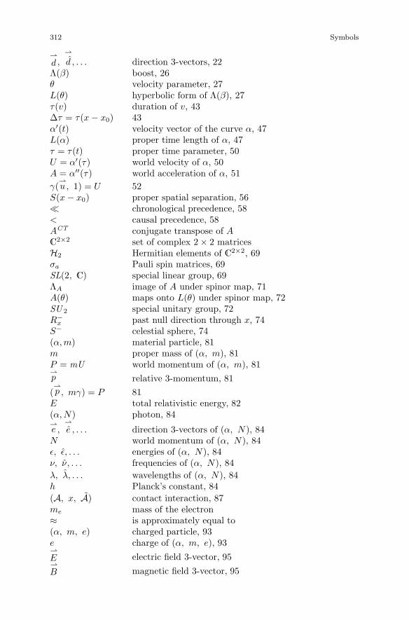
312 Symbols
⇀
d ,⇀
d , . . . direction 3-vectors, 22Λ(β) boost, 26θ velocity parameter, 27L(θ) hyperbolic form of Λ(β), 27τ(v) duration of v, 43Δτ = τ(x − x0) 43α′(t) velocity vector of the curve α, 47L(α) proper time length of α, 47τ = τ(t) proper time parameter, 50U = α′(τ) world velocity of α, 50A = α′′(τ) world acceleration of α, 51γ(
⇀u, 1) = U 52
S(x − x0) proper spatial separation, 56� chronological precedence, 58< causal precedence, 58ACT conjugate transpose of AC2×2 set of complex 2 × 2 matricesH2 Hermitian elements of C2×2, 69σa Pauli spin matrices, 69SL(2, C) special linear group, 69ΛA image of A under spinor map, 71A(θ) maps onto L(θ) under spinor map, 72SU 2 special unitary group, 72R−
x past null direction through x, 74S− celestial sphere, 74(α, m) material particle, 81m proper mass of (α, m), 81P = mU world momentum of (α, m), 81⇀p relative 3-momentum, 81(⇀p , mγ) = P 81
E total relativistic energy, 82(α, N) photon, 84⇀e ,
⇀
e , . . . direction 3-vectors of (α, N), 84N world momentum of (α, N), 84ε, ε, . . . energies of (α, N), 84ν, ν, . . . frequencies of (α, N), 84λ, λ, . . . wavelengths of (α, N), 84h Planck’s constant, 84(A, x, A) contact interaction, 87me mass of the electron≈ is approximately equal to(α, m, e) charged particle, 93e charge of (α, m, e), 93⇀
E electric field 3-vector, 95⇀
B magnetic field 3-vector, 95
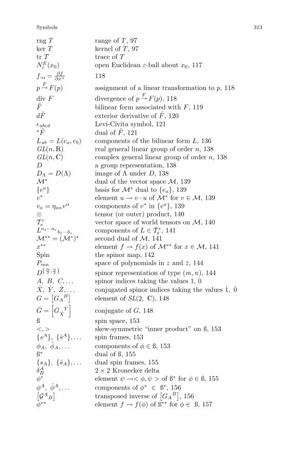
Symbols 313
rng T range of T , 97ker T kernel of T , 97tr T trace of TNE
ε (x0) open Euclidean ε-ball about x0, 117
f,α = ∂f∂xα 118
pF→F (p) assignment of a linear transformation to p, 118
div F divergence of pF→F (p), 118
F bilinear form associated with F , 119dF exterior derivative of F , 120εabcd Levi-Civita symbol, 121∗F dual of F , 121Lab = L(ea, eb) components of the bilinear form L, 136GL(n,R) real general linear group of order n, 138GL(n,C) complex general linear group of order n, 138D a group representation, 138DΛ = D(Λ) image of Λ under D, 138M∗ dual of the vector space M, 139{ea} basis for M∗ dual to {ea}, 139v∗ element u → v · u of M∗ for v ∈ M, 139va = ηaαvα components of v∗ in {ea}, 139⊗ tensor (or outer) product, 140T r
s vector space of world tensors on M, 140La1···ar
b1···bs components of L ∈ T rs , 141
M∗∗ = (M∗)∗ second dual of M, 141x∗∗ element f → f(x) of M∗∗ for x ∈ M, 141Spin the spinor map, 142Pmn space of polynomials in z and z, 144D(m
2 , n2 ) spinor representation of type (m,n), 144
A, B, C, . . . spinor indices taking the values 1, 0X, Y , Z, . . . conjugated spinor indices taking the values 1, 0G =
[GA
B]
element of SL(2, C), 148
G =[G Y
X
]conjugate of G, 148
ß spin space, 153<, > skew-symmetric “inner product” on ß, 153{sA}, {sA}, . . . spin frames, 153φA, φA, . . . components of φ ∈ ß, 153ß∗ dual of ß, 155{sA}, {sA}, . . . dual spin frames, 155δAB 2 × 2 Kronecker delta
φ∗ element ψ →< φ, ψ > of ß∗ for φ ∈ ß, 155φA, φA, . . . components of φ∗ ∈ ß∗, 156[GA
B
]transposed inverse of
[GA
B], 156
φ∗∗ element f → f(φ) of ß∗∗ for φ ∈ ß, 157
314 Symbols
ß = ß × {1} “conjugate” of ß, 157φ (φ, 1) ∈ ß for φ ∈ ß, 157{sX}, {¯sX}, . . . conjugate spin frames, 158φX ,
¯φX , . . . components of φ, 158
G =[GX
Y
]conjugate of G =
[GA
B
], 158
ß∗ dual of ß, 158{sX}, {¯sX}, . . . dual conjugate spin frames, 158φ∗ element of ß∗ conjugate to φ∗ ∈ ß∗, 159φX ,
¯φX , . . . components of φ∗, 159(
r sm n
)valence of a spinor, 159
ξA1···ArX1···XsB1···BmY1···Yn
spinor components, 159
ε =[0 −11 0
]=[ε11 ε10ε01 ε00
]= [εAB] = [εXY ] = εXY , 161
ßrsmn space of spinors of valence
(r sm n
), 164
Ckl(ξ), Ckl(ξ), . . . contractions of ξ, 166, 167ξ spinor conjugate of ξ, 167ξ(AB) symmetrization of ξAB , 168ξ[AB ] skew-symmetrization of ξAB , 169α(AβB) symmetrization of αAβB, 169σa
AX , σaAX Infeld-van der Waerden symbols, 169
V AX spinor equivalent of v ∈ M, 170VAX spinor equivalent of v∗ ∈ M∗, 175FAXBY spinor equivalent of the bilinear form F , 179φAB symmetric spinor determined by FAXBY , 180ξA → eiθξA phase change, 185∇AX spinor differential operator, 197Rn real n-space, 202〈p, q〉 Euclidean inner product on Rn, 202‖p‖ Euclidean norm on Rn, 202Uε(p) open ball of radius ε about p in Rn, 203C∞ smooth, 203Sn n-sphere, 203(U, ϕ) chart, 206χ : U → M coordinate patch, 211χi coordinate velocity vector, 218Tp(M) tangent space to M at p, 218(p, q) Minkowski inner product on R5, 221M5 5-dimensional Minkowski space, 221Γr
ij Christoffel symbols, 230
Symbols 315
H3(r) hyperbolic 3-space, 240R Riemann curvature tensor, 246Rij Ricci tensor, 249R scalar curvature, 249Gij Einstein tensor, 249Tij energy-momentum tensor, 250F∗p derivative of F at p, 252E Einstein static universe, 255F ∗g pullback metric, 260I− past null infinity, 266I+ future null infinity, 266i− past timelike infinity, 273i+ future timelike infinity, 273i0 spacelike infinity, 274dE E-distance, 279NE
ε (x0) open Euclidean ε-ball about x0, 280ME M with the Euclidean topology, 280ClEA, bdyE A, . . . Euclidean closure, boundary,. . . of A ⊆ MC(x) C−
T (x) ∪ C+T (x) ∪ {x}, 284
NPε (x0) P -open ε-ball about x0, 284
MP M with the path topology, 285ClP A, bdyP A, . . . path closure, boundary, . . . of A ⊆ MH(X) homeomorphism group of X , 292[α] homotopy class of the path α, 297α−1 inverse of the path α, 297βα product of the paths α and β, 297π1(X, x0) fundamental group of X at x0, 297π1(X) fundamental group of X , 297(X, p) universal covering manifold of X , 299RP 2 real projective plane, 300Z2 group of integers mod 2RP 3 real projective 3-space, 301RPn real projective n-space, 301SO(3) rotation group, 302

Index
A
aberration formula, 86
accelerations, 38, 48, 49, 82, 201, 228, 230
active transformations, 73, 77, 80
addition of velocities formula, 26
admissible basis, 19
admissible frame of reference, 19
local, 201
nonexistence of, 6
advanced null coordinates, 270
affine parametrization, 262
α-emission, 87
anti-isomorphism, 158
B
barn paradox, 41
bilinear form, 7
components of, 120
matrix of, 120
nondegenerate, 7
skew-symmetric, 119
spinor equivalent of, 192
symmetric, 7
binding energy, 88
binomial expansion, 82, 85, 91
Biot-Savart Law, 127
bivector, 120
spinor equivalent of, 180
boost, 26
C
canonical basis, 107
canonical forms, 107, 109, 195
carriers of a representation, 138
Cartan, E., 135
catenary, 117
causal automorphism, 59, 60, 223, 292
causal precedence, 58
causality assumption, 4
causality relations, 58, 222, 227
Cayley-Hamilton Theorem, 103
change of basis formula, 119
characteristic equation, 99
charge, 93
charge-to-mass ratio, 116
charged particle, 93
Christoffel symbols, 230
chronological precedence, 58
Clock Hypothesis, 48
clocks, 2, 36, 48
atomic, 2
synchronization of, 3
closed
in Rn, 203
in X, 203
commutation relations, 169
Compton effect, 88
Compton wavelength, 90
cone, 4
null, 11, 221, 268
time, 16, 49, 221
configuration space, 302
conformal diffeomorphism, 259
conformal embedding, 260
conformally related metrics, 260
317
318 Index
conjugate isomorphism, 158
conjugate spin covector, 158
conjugate spin vector, 158
conjugate spinor, 158, 168
conjugate transpose, 69
conjugation representation, 146
connectible by a light ray, 14
conservation of energy, 87, 90
conservation of momentum, 81, 87
conservation of 4-momentum, 87
conservation laws, 81, 88
constant curvature, 248, 253
constant electromagnetic fields, 123
constant loop, 297
contact interaction, 87
continuous, 203
contraction, 166
contravariant rank, 141
contravariant vector, 141
coordinate curve, 218
coordinate functions, 50, 202, 203
coordinate patch, 211
coordinate transformation, 219
coordinates
spatial, 2, 10, 29, 253
time, 3, 10, 253
cosmic rays, 23
cosmological constant, 250
cosmological model, 252
Coulomb field, 123
total energy of, 125
covariant rank, 141
covariant vector, 141
covector, 141
covering map, 299
covering transformation, 299
curve, 47, 217
component functions, 47
E-continuous future- (past-) timelike,280
null, 47, 226
reparametrization of, 47
smooth, 47, 217
spacelike, 47, 226
timelike, 47, 226
cylinder, 242
locally flat, 242
D
decay, 87
derivative of a smooth map, 252
de Sitter spacetime, 224
Christoffel symbols for, 231
conformal coordinates, 215
constant curvature, 249
Einstein tensor, 249
geodesics of, 240
global coordinates, 214
hyperbolic coordinates, 217
line element for, 226
Lorentz metric for, 224
null infinity, 266
planar coordinates, 215
Ricci tensor, 249
Riemann curvature tensor, 247
and Robertson-Walker metrics, 254
scalar curvature, 249
diffeomorphism, 203
dilation, 60
time, 22
Dirac
equation, 135, 136
Scissors Problem, 295
direct sum, 43
direction 3-vector, 22
of a photon, 84
of a reference frame, 22
disintegration, 87
displacement vector, 10
null, 10
spacelike, 12
timelike, 12
distance, 57
measured with clocks, 57
divergence, 118
dominant energy condition, 113, 123, 195
Doppler effect, 85
transverse, 85
double cover, 304
dual
basis, 139, 157
of a bivector, 122
duration, 43
E
E-continuous curve, 280
future-timelike, 281
future-timelike at t0, 281
past-timelike, 281
past timelike at t0, 281

Index 319
timelike, 281
timelike vs smooth timelike, 281
E-continuous map, 280
E-distance, 279
E-open ball, 280
E-open set, 280
E-topology, 280
eigenspace, 98
eigenspinor, 190
eigenvalue
of a linear transformation, 98
of a spinor, 190
eigenvector, 98
Einstein field equations, 250
empty space solutions, 250
Einstein static universe, 255
geodesics, 258
line element, 256
Einstein summation convention, xi
electric 3-vector, 95
electromagnetic field, 94, 120
constant, 113, 123
null, 99
regular, 99
spinor, 186
electromagnetic spinor, 186
electromagnetic wave
simple plane, 129
spherical, 3, 17, 35
electron, 88
spin, 135, 294
elevator experiment, 200
energy, 82
Coulomb field, 125
density, 111
of a photon, 84
total relativistic, 82
energy-momentum tensor, 250
energy-momentum transformation, 109
spinor form of, 195
equation of motion, 93
Euler angles, 72
event horizon, 268
events, 1, 9
expanding universe, 255
extended complex plane, 73, 76, 79
exterior derivative, 120
F
Feynman path, 288
Feynman track of an electron, 288
field equations, 198, 250, 255, 277
field of vision, 79
Fizeau procedure, 3
flag pole of a spin vector, 179
4-acceleration, 51
4-momentum
of a material particle, 81
of a photon, 84
4-tensor, 141
4-vector, 169
contravariant, 141
covariant, 141
4-velocity, 50
fractional linear transformation, 73, 77
frame of reference, 3, 10
admissible, 4, 19
free charged particle, 93
free particle, 87
frequency of a photon, 84
fundamental group, 297
of a product, 298
of real projective space, 300, 301
of the rotation group, 303
future-directed
null curve, 47
null vector, 17
timelike curve, 47
timelike vector, 16
future null cone, 17
future null direction, 74
future null infinity, 266, 274
future time cone, 16
future timelike infinity, 273
G
Gaussian curvature, 243
of cylinder, 243
of S2, 243
general linear group, 138
general theory of relativity, 202
geodesic, 230
affine parametrization, 262
causal character, 234
constant speed, 233
degenerate, 230
existence and uniqueness, 232
of de Sitter spacetime, 235
of Minkowski spacetime, 234
of S2, 234
of S3, 235
reparametrization of, 232

320 Index
geodesic hypothesis, 250
gravitation, 6, 199, 249
group representation, 138
H
Hermitian matrix, 170
homeomorphism, 203, 292
homeomorphism group, 292
homomorphism, 14, 138
homotopic paths, 297
homotopy, 297
hyperbolic form of special Lorentztransformations, 27
hyperbolic motion, 55
I
identity representation, 138, 141, 146
index of an inner product, 9
inelastic collision, 90
inertial mass, 81
Infeld-van der Waerden symbols, 173
initial point on a worldline, 87
inner product, 7
indefinite, 7
index of, 9
Lorentz, 9
negative definite, 7
positive definite, 7
instantaneous rest frame, 53
invariant subspace
of a linear transformation, 99
of a representation, 143
Inverse Function Theorem, 208
isometry, 252
K
Kennedy-Thorndike experiment, 3
kernel, 68, 97
L
length, 39contraction, 40
Levi-Civita symbols, 121
spinor equivalent of, 196light cone, 11
future and past, 17
light ray, 11as an intersection of null cones, 11
light signals, 3, 17
light travel time, 3lightlike vector, 10
line element, 225loop, 297
constant (trivial), 297
Lorentz contraction, 40invisibility of, 79
Lorentz 4-Force Law, 93
Lorentz group, 19general homogeneous, 14
inhomogeneous, 19
2-valued representations of, 142, 144Lorentz inner product, 9
spinor equivalent of, 192
Lorentz invariant, 99, 136, 141Lorentz transformations, 14, 19
boost, 26
decomposition of, 28determined by three past null directions,
79
effect on past null directions, 79general homogeneous, 14
hyperbolic form, 27
improper, 19invariant null directions, 79
nonorthochronous, 15
orthochronous, 15proper, 19
special, 25
vs fractional linear transformations, 77Lorentz World Force Law, 93
lowering indices, 162
M
magnetic 3-vector, 95
manifold, 206
complete, 238n-dimensional, 206
smooth, 206
Index 321
mass
inertial, 81
proper, 81
relativistic, 82mass-energy equivalence, 83
massless free-field equations, 198, 277
material particle, 81
worldline of, 47free, 81
matrix group, 137
order of, 137
representation of, 138matrix of a bilinear form, 120
Maxwell’s equations, 118, 122
solutions of, 123, 124, 129, 130
spinor form of, 197measuring rods, 39, 40
metric, 219
component functions, 219
Lorentzian, 220Riemannian, 219
Michelson-Morley experiment, 3
Minkowski diagram, 32, 266
Minkowski spacetime, 9multilinear functional, 140, 159
N
neutrino equation, 198
null basis, 10
null cone, 11future, 17
past, 17
null direction, 61
future, 74past, 74
null electromagnetic field, 99
null flag, 185
null vector, 10future-directed, 17
parallel, 10
past-directed, 17
orthogonal, 10null worldline, 11
O
observer, 1
admissible, 1
open
in Minkowski spacetime, 117
in Rn, 203
in X, 203
orientation-entanglement relation, 304
orthochronous, 15
orthogonal complement, 7
orthogonal transformation, 12, 222
and causal automorphisms, 60, 227
and fractional linear transformations, 77
and homeomorphisms, 292
associated matrices, 13
invariant null directions, 79
orthochronous, 60
orthogonality, 7
of null vectors, 10
of spacelike and null vectors, 58
of spacelike vectors, 57
with timelike vectors, 15
orthonormal basis, 8
outer product, 165
P
P-continuous curve, 289
characterized as Feynman paths, 289
vs E-continuous curves, 288
vs timelike curves, 288
P-open set, 284
not E-open, 284
paradox
barn, 41
twin, 36
parallel postulate, 235
parity nonconservation, 198
particle
charged, 93
free, 87
free charged, 93
horizon, 268
material, 81
passive transformation, 73
past-directed
null curve, 47
null vector, 17
timelike curve, 47
timelike vector, 16
past null cone, 17
past null direction, 74
past null infinity, 266, 274
past time cone, 16
past timelike infinity, 273
322 Index
path, 296
inverse of, 297
products of, 297
path connected, 296
path topology, 284
basis for, 285
homeomorphisms of, 292
topological properties, 286
Pauli spin matrices, 69
Penrose diagram, 266
phase factor, 182
photon, 84
direction 3-vector of, 84
energy, 84
4-momentum of, 84
frequency, 84
propagation of, 2
wavelength, 84
worldline, 4, 11
world momentum of, 84
pions, 36
Planck’s constant, 84
Poincare group, 19
point event, 1
Poynting 3-vector, 111
principal null directions, 108, 109
product path, 297
proper mass, 81
proper spatial separation, 56
proper time function, 50
proper time parameter, 227
proper time separation, 44
pullback, 260
Pythagorean Theorem, 58
Q
quadratic form, 7
quantum mechanics, 88, 142, 198, 294
R
raising indices, 162
range, 97
rank
contravariant, 141
covariant, 141
real projective n-space, 301
fundamental group of, 301
regular electromagnetic field, 99
relative 3-momentum, 81
relativistic electron, 137
relativistic energy, 82
relativistic mass, 82
relativity
of simultaneity, 23
principle, 5
representations, 138
carriers of, 138
equivalent, 143
irreducible, 143
reducible, 143
spinor, 145
two-valued, 144
retarded null coordinates, 270
reversed Schwartz inequality, 44
reversed triangle inequality, 44
Ricci flat, 250
Ricci tensor, 249
Riemann curvature tensor, 246
Riemann sphere, 73
rigidity, 40
Robb’s theorem, 57
Robertson-Walker metrics, 254
rocket twin, 37, 55
rotation group, 302
rotation in the Lorentz group, 20
rotation subgroup, 20
S
Schur’s lemma, 143
Schwartz inequality
for R3, 10
reversed, 44
signals, 3, 33, 57, 268
simply connected, 298
simultaneity, 23
relativity of, 23
simultaneous, 23
skew-symmetric bilinear form, 119
skew-symmetric linear transformation, 94
null, 99
regular, 99
skew-symmetrization, 169
smooth
assignment, 118
map, 203
real-valued function, 203
vector field, 118

Index 323
spacelike displacement, 57
spacelike infinity, 274spacelike vector, 12
spacetime, 220
spatially homogeneous and isotropic, 252spatial coordinates, 29, 254
special linear group, 69special Lorentz transformation, 25
hyperbolic form, 27speed
of light, 3of material particles, 82
spin, 88, 135, 137
spin covector, 155spin frame, 153
spin space, 153spin transformation, 69
spin vector, 153spinor, 135
components of, 159
conjugate, 158, 168contravariant indices, 159
covariant indices, 159dotted indices, 159
electromagnetic field, 186equivalents (See spinor equivalent)
essential two- valuedness of, 185, 293form of Maxwell’s equations, 198
Hermitian, 168
lower indices, 159skew-symmetric, 168
symmetric, 168undotted indices, 159
upper indices, 159valence of, 159
spinor-covector, 172
spinor equivalentof a bilinear form, 192
of a bivector, 180of a covector, 176
of differential operators, 197of the dual of a bivector, 196
of a 4-vector, 172of Levi-Civita symbols, 196
of the Lorentz inner product, 192
of a vector, 172of a world vector, 172
spinor map, 71spinor representation, 145
type of, 145spinorial object, 142, 293, 305
standard configuration, 25
stereographic projection, 75stress tensor, 111
subgroup
of the Lorentz group, 19, 20, 24
of transformations, 72, 138
summation convention, xi
symmetric linear transformation, 110
symmetrization, 168
synchronization, 2
lack of, 36
T
tangent space, 218, 219
tangent vector, 47, 217
temporal order, 2, 4, 34, 56
tensor product, 140
tensorial objects, 303
terminal point of a worldline, 87
3-vector
direction, 22
relative momentum, 81
velocity, 21, 52, 85
time
axis, 43
cone, 16
coordinates, 3
dilation, 22, 36
orientation, 16
in units of distance, 3
timelike curve
E-continuous, 281
smooth, 47
timelike straight line, 43
timelike vector, 12
future-directed, 16
past-directed, 16
timelike worldline, 47
topological manifold, 296
products of, 298
topology
Euclidean (or E-), 280
fine, 279
path (or P-), 284
total 4-momentum, 87
total relativistic energy, 82
total world momentum, 87
trace, 109
trace free, 110
transformation equations, 40, 206, 246
transformation matrix, 13, 137
translation, 4, 60
324 Index
translation of a light ray, 61lifts of, 62
twin paradox, 362-form, 120
U
uniformly moving charge, 125
unit vector, 8unitary matrix, 72universal covering manifold, 299
V
vector field, 118components of, 118smooth, 118
velocity parameter, 27velocity 3-vector, 21, 52, 85velocity vector, 47, 217version, 304
W
wave equation, 132
wave function, 142, 294, 305
wavelength of a photon, 84
weak interaction, 198
Weyl, 1
neutrino equation, 198
world acceleration, 51
world momentum
of a material particle, 81
of a photon, 84
world tensor, 136, 141
world vector, 169
worldline, 1
of a material particle, 47
of a photon, 4, 11
Z
Zeeman’s Theorem, 60, 227, 292


