Download - Multiscale adjoint waveform tomography for surface …€¦ · · 2015-09-10Multiscale adjoint waveform tomography for surface ... of fundamental-mode and overtone SWs via a mode-branch

Multiscale adjoint waveform tomography for surfaceand body waves

Yanhua O. Yuan1, Frederik J. Simons1, and Ebru Bozdağ2

ABSTRACT

We have developed a wavelet-multiscale adjoint scheme forthe elastic full-waveform inversion of seismic data, includingbody waves (BWs) and surface waves (SWs). We start the in-version on the SW portion of the seismograms. To avoid cycleskipping and reduce the dependence on the initial model ofthese dispersive waves, we commence by minimizing anenvelope-based misfit function. Subsequently, we proceed tothe minimization of a waveform-difference (WD) metric appliedto the SWs only. After that, we fit BWs and SWs indiscrimi-nately using a WD misfit metric. In each of these three steps,we guide the iterative inversion through a sequence of nestedsubspace projections in a wavelet basis. SW analysis preservesa wealth of near-surface features that would be lost in conven-

tional BW tomography. We used a toy model to illustrate thedispersive and cycle-skipping behavior of the SWs, and to in-troduce the two ways by which we combat the nonlinearity ofwaveform inversions involving SWs. The first is the wavelet-based multiscale character of the method, and the second theenvelope-based misfit function. Next, we used an industry syn-thetic model to perform realistic numerical experiments to fur-ther develop a strategy for SW and joint SW as well as BWtomography. The effect of incorrect density information onwave-speed inversions was also evaluated. We ultimately for-malize a flexible scheme for full-waveform inversion basedon adjoint methods that includes BWs and SWs, and also con-siders P- and S-wave speeds, as well as density. Our method isapplicable to waveform inversion in exploration geophysics,geotechnical engineering, regional, and global seismology.

INTRODUCTION

Near-surface heterogeneities are responsible for complex scatter-ing and mode conversions. Characterizing near-surface hetero-geneity is crucial for statics corrections and to analyze wavepropagation in the deep structure. Rayleigh and Love waves accountfor the bulk of the energy in the seismic wavefield — two-thirds ofthe total energy input by a circular footing vibrating harmonicallyover a homogeneous isotropic elastic half-space (Miller and Pursey,1955). The energy of surface waves (SWs) is dissipated proportion-ally to the distance from the source (Rayleigh, 1885), whereas thebody-wave (BW) energy decay scales with the square of distancetraveled in the whole space, and even faster near the free surface(Ewing et al., 1957; Richart et al., 1970). Thus, at some distancefrom the source, the seismic wavefield is essentially dominated bySWs. Unlike BWs, which may penetrate to great depths, SW propa-gation paths are concentrated to depths that are on the order of their

wavelength (Dahlen and Tromp, 1998). Especially for S-wavevelocities, SWs provide strong constraints on near-surface structure.Despite this, SWs (“ground roll”) are most commonly removed inexploration-scale industry applications (Dobrin and Savit, 1988),which not only deprives the records of a certain amount of infor-mation, but also tends to introduce errors through transformationand filtering. In global seismology and mantle tomography, “crustalcorrections” (Bozdağ and Trampert, 2008) mutatis mutandis play arole equivalent to SW removal. Involving the SWs in seismictomography eliminates the burdensome step of their removal in pre-processing, and treats them for the signal that they are.

Surface waves: Applications

SW analysis has a long history in global seismology (Wood-house, 1974) and exploration geophysics (McMechan and Yedlin,1981), and it is now widely embraced as a valuable tool to conduct

Manuscript received by the Editor 3 October 2014; revised manuscript received 15 May 2015; published online 17 August 2015.1Princeton University, Department of Geosciences, Princeton, New Jersey, USA. E-mail: [email protected]; [email protected]é de Nice, GéoAzur, Sophia-Antipolis, France. E-mail: [email protected].© 2015 Society of Exploration Geophysicists. All rights reserved.

R281

GEOPHYSICS, VOL. 80, NO. 5 (SEPTEMBER-OCTOBER 2015); P. R281–R302, 18 FIGS.10.1190/GEO2014-0461.1

subsurface characterization (Socco and Strobbia, 2004; O’Neill andMatsuoka, 2005; Socco et al., 2010) in different research fields, in-cluding geotechnical and geoenvironmental engineering (Foti,2000; Rix et al., 2001). SW analysis may be more important eventhan other popular methods such as refraction or resistivity surveysor magnetic imaging (Crice, 2005). SW can characterize a mediumat large (e.g., in regional and global seismology, to determine thestructure of the earth’s crust and upper mantle), intermediate (e.g.,in exploration geophysics, to constrain near-surface structure, or tocorrect statics; or in geotechnical engineering, to infer the shearstiffness of the ground materials), and even at the smallest scales,for the nondestructive evaluation of engineering materials (e.g., us-ing ultrasonic SWs to detect material defects; Thompson and Chi-menti, 1997; Bagheri et al., 2014).Known by their acronyms SWA, SASW, or MASW, surface-

waves analysis and spectral or multichannel analysis (Park et al.,1999) of surface waves are now widely used methods for seismicsite characterization in geotechnical engineering, which values theirnoninvasive nature, good resolution at shallow depth, and efficiencyin time and cost. The methods have been developed greatly duringthe past few decades. Tokimatsu et al. (1992) recognized the effectsof higher modes in some types of soil profiles, when the S-wavespeed profile is not increasing regularly with depth. Foti (2000)used a multistation method for the robust determination ofdispersion curves. Other variants of SW dispersion analysis includef-k (Capon, 1969), τ-p (Buland and Chapman, 1983), and spatialautocorrelation (Aki, 1957) methods. Multichannel methods (Milleret al., 1999; Pratt and Shipp, 1999) have been proposed to improvedata quality control under the influence of noise. A variety of inver-sion algorithms (Yuan and Nazarian, 1993; Xia et al., 1999; Rix et al.,2001) have been developed for determining S-wave speed profilesfrom dispersion curves. In addition to the estimation of stiffness pro-files, e.g., for pavement system evaluation and site characterization,SW analysis has been used to obtain in situ material damping ratioprofiles for general site investigations either separately (Rix et al.,2000; Xia et al., 2002) or simultaneously (Lai and Rix, 1998; Foti,2000) by considering the coupling between phase velocity and at-tenuation as part of two-station or multistation methods.In regional and global seismology, the variation of the propaga-

tion speeds of long-period SWs has been observed and interpretedfor the study of crustal and upper-mantle structure for decades (e.g.,Woodhouse, 1974; Woodhouse and Dziewoński, 1984; Capdevilleand Cance, 2015). By the 1980s, efforts to use SW dispersion andphase-velocity measurements at long periods to constrain regionaland global-scale mantle S-wave structure, including its anisotropy,using tomographic techniques were very well established (Mon-tagner and Nataf, 1988; Montagner and Jobert, 1988; Snieder,1988a, 1988b). To name but a few additional examples: overtoneSWs were used by Cara et al. (1984) and Lévêque and Cara(1985) to provide evidence for upper mantle anisotropy. Nolet et al.(1986) formalized a waveform-fitting approach using the conjugategradient method for Love and Rayleigh waves. Stutzmann andMontagner (1993, 1994) extended the use of higher modes of SWsto study structure in the transition zone. Ekström et al. (1997)mapped phase velocity by minimizing dispersion residuals of fun-damental Love and Rayleigh waveforms, isolated from interferingovertones via phase-matched filters. Van Heijst and Woodhouse(1999) measured global high-resolution phase velocity distributionsof fundamental-mode and overtone SWs via a mode-branch strip-

ping technique (van Heijst and Woodhouse, 1997). Trampert andWoodhouse (2003) used fundamental-mode SWs to map aniso-tropic phase velocities. After S20RTS, Ritsema et al. (2011)developed S40RTS, a shear-velocity model of the mantle, usingRayleigh-wave dispersion, normal-mode splitting function, andS-wave traveltime measurements. Even as (high frequency) BWstudies generally yield sharper tomographic images (Rawlinsonand Sambridge, 2003; Romanowicz, 2003; Nolet, 2008), (low fre-quency) SWs have contributed greatly to our understanding of thelong-wavelength internal structure of the earth. In some areas, suchas beneath the ocean basins, they are crucial to increase vertical res-olution, or to make up for insufficient sampling in regions with poorray coverage due to lack of stations (Romanowicz and Giardini,2001; Simons et al., 2006b).In hydrocarbon exploration, seismic techniques have generally

been based on BW propagation, in particular P-wave reflections.In contrast, SWs, despite their preponderance in the seismic record,are usually considered as coherent noise masking the reflections,hence to be removed by recording and processing procedures(e.g., Dobrin and Savit, 1988). In seismic exploration, McMechanand Yedlin (1981) extracted dispersion curves of Rayleigh wavesfrom common-shot marine seismic profiles based on slant stackingfollowed by 1D Fourier transformation. Gabriels et al. (1987) de-termined S-wave velocities in sediments to a depth of 50 m bymeans of higher mode Rayleigh waves. The industry is increasinglyrecognizing the value of SWs for seismic inversions. Some exam-ples: Ivanov et al. (2006) showed that a reference model derivedfrom SW S-wave speed estimation reduces the nonuniqueness ofthe refraction inversion problem. Gouédard et al. (2012) combinedSW eikonal tomography and crosscorrelation methods for phasearrival-time estimation for velocity analysis of a strongly hetero-geneous and scattering medium in a hydrocarbon-exploration set-ting. Droujinine et al. (2012) developed an integrated workflowwith dispersion curve and full-waveform inversion to retrieve com-plex shallow structure, as needed for the accurate imaging of deepertargets.

Surface waves: Methods and challenges

Most of the applications of SWs in different disciplines operateon the same principle, which is to estimate a set of dispersion curvesfrom the data, and subsequently, to solve an inverse problem forelastic or anelastic parameters (Haskell, 1953; Stokoe et al.,2004; O’Neill and Matsuoka, 2005). SW analysis and its applica-tions have their challenges. First, the success of SW dispersion-curve inversion depends on the clear separation of fundamentaland higher modes, which can be realized only if very dense spatialsampling and long acquisition spreads are used (Socco and Strob-bia, 2004). Many strategies in acquisition and processing have beendeveloped to help identify and separate different modes (Lai andRix, 1999; Beaty et al., 2002; O’Neill and Matsuoka, 2005); how-ever, several authors (e.g., Zhang and Chan, 2003; Maraschini et al.,2010; Socco et al., 2010) show that mode misidentification is noteasy to avoid and may produce significant errors. Second, SWdispersion-curve inversions usually do not consider the effect of3D inhomogeneity in the medium, until many of them are combinedto produce the lateral variations that are precisely the target also inexploration applications. In regional and global seismology, 1Dprofiles are jointly inverted to recover 2D or 3D lateral hetero-geneities (Woodhouse, 1974; Nataf et al., 1986; Nolet, 1990). 1D

R282 Yuan et al.

reference models, such as the Preliminary Reference Earth Model(Dziewoński and Anderson, 1981) are a good starting point formatching SW observations relatively easily.As an alternative, full-waveform inversion of SWs considers the

propagation of SWs in a realistically heterogeneous medium(Snieder, 1988b), in which case the separation of different modesand the prior estimation of dispersion curves are not necessary.Even in that case, due to their strongly dispersive nature, the com-plex interference of fundamental and higher modes and the potentialfor cycle skipping, particularly when an adequate initial estimate isnot available, SWs are much more difficult to handle than BWs. Inaddition to these complications, the low-frequency ground motionmay not be very well recorded in industry applications.Cycle skipping causes local minima in the inversion (VanDecar

and Crosson, 1990). Frequency-dependent phase measurementsbased on crosscorrelations of predicted and observed SWs, andlayer-stripping approaches (Pratt et al., 1996) are designed to mit-igate cycle-skipping problems of SW tomography (Lebedev et al.,2005; Sigloch and Nolet, 2006). Another possible solution to thenonlinearity problem is to use a multiscale approach (Bunks et al.,1995; Sirgue and Pratt, 2004; de Hoop et al., 2012; Yuan and Si-mons, 2014), proceeding from large (low frequencies) to smallscales (high frequencies) in the seismograms, progressively involv-ing higher (temporal) frequencies. Prieux et al. (2013a, 2013b) andOperto et al. (2013) discuss strategies to reduce the nonlinearity ofthe elastic multiparameter inversion with multicomponent data andto control the trade-off between parameters by hierarchically select-ing the data components to invert and the parameter classes to up-date. Brossier et al. (2009) use a frequency-domain preconditioningscheme equivalent to time-domain damping to stabilize elastic in-version. Shin and Cha (2008) transform the wavefield to the Laplacedomain to reduce the sensitivity on the initial model. Pérez Solanoet al. (2014) use a windowed-amplitude waveform inversion methodin the Fourier domain for near-surface imaging using SWs.

Surface waves: A new approach

Reducing the nonlinearity of waveform inversion problems in-volves a judicious choice of the objective function (Luo and Schus-ter, 1991; Gee and Jordan, 1992; Dahlen and Baig, 2002; Fichtneret al., 2008; Bozdağ et al., 2011; Rickers et al., 2012; Masoni et al.,2014). Bozdağ et al. (2011), in particular, discuss several misfitfunctions in seismic tomography. Among those, we develop theenvelope-based objective function to measure SWs in this study.The extraction of envelopes from SWs through the Hilbert trans-form greatly reduces the nonlinearity of waveform inversion bythe separation of phase and amplitude information.In this paper, we explore the sensitivity of SWs in waveform in-

version to estimate near-surface structure. To address the problems ofcycle skipping in the waveform fitting, we develop a strategy basedon a wavelet-multiscale approach, newly combined with an envelope-difference (ED) misfit functional (Yuan et al., 2014). We are moti-vated by the intrinsic multiresolution property of the wavelet trans-form (Mallat, 1989), which provides a simple and natural frameworkfor interpreting signals at different levels of detail. Goals similar tothose that we aim to achieve in this study could possibly be achievedvia traditional, convolutional, or Fourier-domain time-frequency fil-tering approaches (e.g., Pratt, 1999; Sirgue and Pratt, 2004; Fichtneret al., 2013; Prieux et al., 2013a). In this study, we focus exclusivelyon wavelet-based time-scale analysis. Temporal scales of the seismo-

grams illuminate spatial scales in the subsurface structure, but ofcourse the correspondence is not exact in any basis: specific sub-bands of the time-domain seismograms do not map to the same sub-bands of the space-domain structure (see, e.g., Beylkin, 1992; Ecoub-let et al., 2002).Our work should be considered as an extension to our previous pa-

per (Yuan and Simons, 2014), in which we introduced a multiresolu-tion technique to adjoint-based seismic tomography (e.g., Fichtner,2011; Luo et al., 2014), but which excluded SWs (but we includedall reflected, refracted, transmitted BW phases, and multiples). Weused time-domain wavelet-based constructive approximation to pro-gressively model smaller scale features in the seismogram. We treatedSWs as noise and removed them using low pass and dip filtering in ourpreprocessing procedure before performing the inversions, as incommon industry practice. In the present paper, we compare the sen-sitivities of SWs and BWs in full-waveform inversions, and we discussstrategies to combine both of them for elastic inversions. Furthermore,we also discuss the effects of incorrect density information on elasticparameter estimation. Finally, we formalize a flexible workflow to real-ize the goal of truly “full”-waveform inversion, in the form of an iter-ative adjoint tomography method that considers density- and elastic-wavespeed variations, and which treats SWs separately in a first stepbefore conducting a joint analysis of SWs and BWs in the sec-ond stage.

MATHEMATICAL PRELIMINARIES

For the development of our method, we rely on two mathematicaltransforms, the wavelet transform and the Hilbert transform, whichwe briefly introduce here.

Wavelet transform

Readers not familiar with the wavelet transform may wish to con-sult the early work of Morlet et al. (1982a, 1982b), in this journal, orthe textbooks by Daubechies (1992), Strang and Nguyen (1997),Mallat (2008), or Jensen and la Cour-Harbo (2001) before reading on.For a given input signal sðtÞ, we first choose a particular wavelet

basis (see Yuan and Simons, 2014). We consider two sets of scaling

functions, ~ϕjk for the analysis and ϕ

jk for the synthesis, as well as two

sets of wavelet functions ~ψjk for analysis and ψ

jk for synthesis, where

j ¼ 1; : : : ; J indicates the scale, J is the maximal decompositiondepth, and k is a measure of the translation in time. The genericsignal sðtÞ can be represented as the sum over all translates kand scales j ¼ 1; : : : ; J, in the expansion

sðtÞ ¼Xk

aJkϕJkðtÞ þ

XJj¼1

Xk

djkψjkðtÞ; (1)

and a partial reconstruction to scale j, leading to a constructiveapproximation, is

sjðtÞ¼Xk

aJkϕJkðtÞþ

XJj 0¼jþ1

Xk

dj0k ψ

j0k ðtÞ¼

Xk

ajkϕjkðtÞ; (2)

where the scaling (approximation, low frequency, and low pass) andwavelet (detail, high frequency, and high pass) coefficients, respec-tively, whatever the algorithmic implementation, are given by

Wavelet multiscale SW tomography R283

aJk ¼ hs; ~ϕJki; and djk ¼ hs; ~ψk

ji: (3)

Hilbert transform

Following Claerbout (1992), the analytic signal of a real-valuedsignal sðtÞ can be expressed as

saðtÞ ¼ sðtÞ þ iHfsðtÞg ¼ EðtÞeiϕðtÞ; (4)

where HfsðtÞg is the Hilbert transform of the real signal sðtÞ andϕðtÞ and EðtÞ stand for the instantaneous phase and the instantane-ous amplitude (or envelope) of the analytic signal, respectively,

ϕðtÞ ¼ arctanHfsðtÞgsðtÞ ; (5)

EðtÞ ¼ffiffiffiffiffiffiffiffiffiffiffiffiffiffiffiffiffiffiffiffiffiffiffiffiffiffiffiffiffiffiffiffiffiffis2ðtÞ þH2fsðtÞg

q: (6)

The separation of phase and amplitude information via the Hilberttransform can be carried out via the fast Fourier transform, sup-pressing negative frequencies. Additional details can be found inMallat (2008). We now list two properties of the Hilbert transformthat will be used later.The derivative of the Hilbert transform of a real signal sðtÞ is the

Hilbert transform of the derivative of sðtÞ:

δHfsðtÞg ¼ H½δfsðtÞg�: (7)

The Hilbert transform is an anti-self-adjoint operator. For two realsignals sðtÞ and uðtÞ, we have

hHfsðtÞg; uðtÞi ¼ −hsðtÞ;HfuðtÞgi: (8)

A MOTIVATING EXAMPLE

The inversion of waveforms that contain SWs greatly increasesthe nonlinearity of full-waveform inversion. Even a small perturba-tion, especially in S-wave speed structure, to a homogeneous back-ground, will cause dispersion, turning a simple SW pulse into acomplicated wavetrain.We designed a simple 2D toy model to illustrate the dispersion and

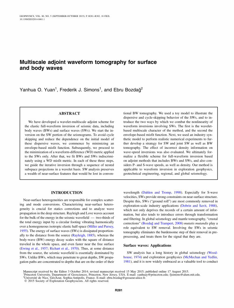
cycle-skipping behavior of SWs. Consider a homogeneous P-wavespeed (VP ¼ 2000 m∕s) and density (ρ ¼ 1200 kg∕m3) model.The S-wave speed model shown in Figure 1a consists of a homo-geneous background shear velocity VS0 ¼ 800 m∕s and an anoma-lous layer of VS1 ¼ 1000 m∕s. The model measures 400 m in thehorizontal direction with 79 uniform mesh nodes (quadrangles in2D), and it is 100 m in the vertical direction with 19 uniform nodes.A total of ð79 × 4þ 1Þ × ð19 × 4þ 1Þ ¼ 24; 409 unique grid pointsand 79 × 19 × ð4þ 1Þ2 ¼ 37; 525 S-wave speeds are used for 2Dspectral element discretization with polynomial degree four (Koma-titsch et al., 2005). The quadrangle mean spacing is 5.3 m.We model horizontal and vertical components of the displace-

ment seismograms using SPECFEM2D, a 2D spectral-elementcode (Komatitsch and Vilotte, 1998). A force is imposed normallyto the surface with a 40-Hz Ricker wavelet, located at 50 m hori-

zontally from the left edge and at 0.5 m in depth. We use a total of401 receivers located at 0.5 m depth and spaced 1 m apart. We alsoconsider a homogeneous S-wave speed model, where VS0 ¼VS1 ¼ 900 m∕s, as an “initial model” for the purpose of ournumerical evaluation, in which we implement SPECFEM2D to com-pute synthetics with the same source-receiver geometry.

Dispersion of surface waves

The dispersive nature of the SWs, waves of different wavelengthsthat travel with different speeds, is manifest by the drawn-out com-plex shapes of the waveform in the target model (Figure 1b and 1d)as compared with the waveforms in a homogeneous background(Figure 1c and 1e).Horizontal components of the SWs are shown as recorded at a

horizontal distance of 350 m from the left edge. The inclusionof the anomalous S-wave layer in the toy model causes the modeledSW to be dispersive. In contrast, the SW trace predicted in a homo-geneous initial model is nondispersive. Figure 1b and 1c shows full-resolution seismograms and their envelopes, whereas Figure 1d and1e shows their approximation after partial reconstruction to scale 8using a Daubechies (1988) wavelet basis (“D12” or “db6” with six“vanishing moments,” see Daubechies, 1992; Strang and Nguyen,1997; Jensen and la Cour-Harbo, 2001). The number of vanishingmoments is one more than the degree of polynomials that can berepresented by the scaling functions without contributions from thewavelets.The traditional analysis of SW would produce dispersion curves

relating measured phase or group velocities to their dominant periodand then invert those for an average 1D S-wave speed profile. In thepresence of 2D or 3D lateral heterogeneity, such procedures wouldbecome necessarily very complex, although they have been a stapleof waveform analysis for many decades.

Cycle skipping of surface waves

Waveform inversions starting from an inadequate initial modelrun the risk of convergence to a secondary minimum becausethe phase difference between observation and prediction may ex-ceed half the period. Such cycle-skipping problems are more severewith a dispersive SW than with BW waveforms. To combat suchnonlinearities, we previously developed a wavelet multiscale strat-egy for BW waveform inversion, in which the initial breakdown ofthe traces to the coarsest scales effectively linearized the inversionproblem (Yuan and Simons, 2014). In this paper, we elaborate onthis framework but, this time, we include the inversion of fre-quency-dependent SW waveforms.Figure 1d and 1e shows the SW waveforms projected onto scale

8, our largest decomposition level in a basis using D12 wavelets.Although the discrepancy between the target and the initial SWwaveforms (thick black lines) is clearly much smaller at thislarge-scale projection than at the original full resolution shownin Figure 1b and 1c, it remains too challenging to attempt waveformfitting with the mean-squared difference as a measure of distance tobe minimized.Thus, to further combat cycle skipping and other confounding

effects caused by the highly oscillatory nature of SW phases evenin this simple toy model, we propose to take the Hilbert transform ofthe waveforms and work with the amplitude information containedin their envelopes (dashed lines in Figure 1) before attempting to

R284 Yuan et al.

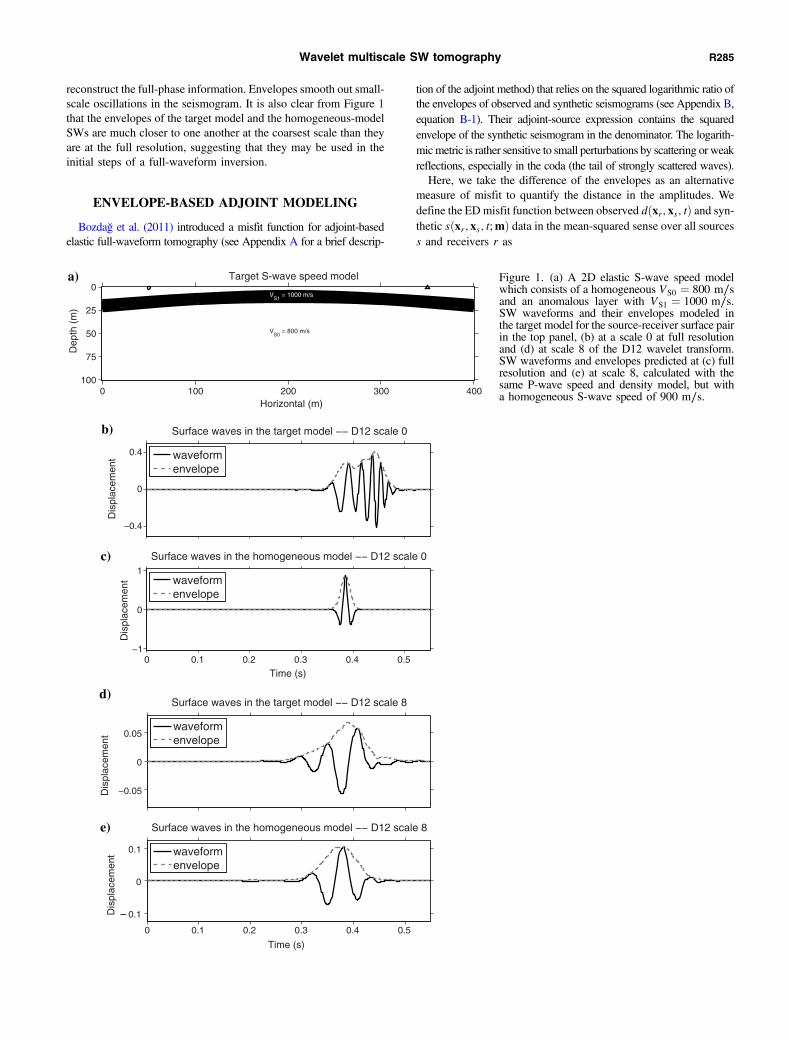
reconstruct the full-phase information. Envelopes smooth out small-scale oscillations in the seismogram. It is also clear from Figure 1that the envelopes of the target model and the homogeneous-modelSWs are much closer to one another at the coarsest scale than theyare at the full resolution, suggesting that they may be used in theinitial steps of a full-waveform inversion.

ENVELOPE-BASED ADJOINT MODELING

Bozdağ et al. (2011) introduced a misfit function for adjoint-basedelastic full-waveform tomography (see Appendix A for a brief descrip-

tion of the adjoint method) that relies on the squared logarithmic ratio ofthe envelopes of observed and synthetic seismograms (see Appendix B,equation B-1). Their adjoint-source expression contains the squaredenvelope of the synthetic seismogram in the denominator. The logarith-micmetric is rather sensitive to small perturbations by scattering or weakreflections, especially in the coda (the tail of strongly scattered waves).Here, we take the difference of the envelopes as an alternative

measure of misfit to quantify the distance in the amplitudes. Wedefine the ED misfit function between observed dðxr; xs; tÞ and syn-thetic sðxr; xs; t;mÞ data in the mean-squared sense over all sourcess and receivers r as

VS0

= 800 m/s

VS1

= 1000 m/s

Horizontal (m)

Dep

th (

m)

Target S-wave speed model

0 100 200 300 400

0

25

50

75

100

−0.4

0

0.4

Dis

plac

emen

t

Surface waves in the target model −− D12 scale 0

waveformenvelope

0 0.1 0.2 0.3 0.4 0.5−1

0

1

Time (s)

Dis

plac

emen

t

Surface waves in the homogeneous model −− D12 scale 0

waveformenvelope

−0.05

0

0.05

Dis

plac

emen

t

Surface waves in the target model −− D12 scale 8

waveformenvelope

0 0.1 0.2 0.3 0.4 0.5

− 0.1

0

0.1

Time (s)

Dis

plac

emen

t

Surface waves in the homogeneous model −− D12 scale 8

waveformenvelope

a)

b)

c)

d)

e)

Figure 1. (a) A 2D elastic S-wave speed modelwhich consists of a homogeneous VS0 ¼ 800 m∕sand an anomalous layer with VS1 ¼ 1000 m∕s.SW waveforms and their envelopes modeled inthe target model for the source-receiver surface pairin the top panel, (b) at a scale 0 at full resolutionand (d) at scale 8 of the D12 wavelet transform.SW waveforms and envelopes predicted at (c) fullresolution and (e) at scale 8, calculated with thesame P-wave speed and density model, but witha homogeneous S-wave speed of 900 m∕s.


χ1ðmÞ ¼ 1

2

Xs;r

ZT

0

kEsðxr; xs; t;mÞ − Edðxr; xs; tÞk2dt; (9)

where T is the window length. We use the symbol k · k throughoutto denote the norm of single-component (s; d) or multicomponent(s; d) seismograms, which we distinguish (by font weight) only inAppendix A. Because EsðtÞ and EdðtÞ are the envelopes of the syn-thetic sðtÞ and the observed data dðtÞ, respectively, they are ob-tained via Hilbert transformation as

Esðxr; xs; t;mÞ ¼ffiffiffiffiffiffiffiffiffiffiffiffiffiffiffiffiffiffiffiffiffiffiffiffiffiffiffiffiffiffiffiffiffiffis2ðtÞ þH2fsðtÞg

q; (10)

Edðxr; xs; tÞ ¼ffiffiffiffiffiffiffiffiffiffiffiffiffiffiffiffiffiffiffiffiffiffiffiffiffiffiffiffiffiffiffiffiffiffiffid2ðtÞ þH2fdðtÞg

q: (11)

Gradient-based methods (see Tarantola, 1984a, 1984b; Trompet al., 2005) require the derivative with respect to the model param-eters of the misfit function χ1ðmÞ in equation 9, which we express interms of δEs, the perturbation in the envelopes of the synthetics dueto a perturbation of the current model δm:

δχ1ðmÞ ¼Xs;r

ZT

0

½Esðxr;xs; t;mÞ−Edðxr;xs; tÞ�δEsðxr;xs; t;mÞdt:

(12)

To avoid notational clutter, we drop the dependence on the space,time, and model coordinates xr, xs, t, and m, and write

δEs ¼sδsþ ½Hfsg�δ½Hfsg�

Es; (13)

where δs and δ½Hfsg� are the perturbations to the synthetic seismo-gram s and its Hilbert transform Hfsg due to a model perturba-tion δm.We introduce the first of three possible envelope ratios (see Ap-

pendix B for the other two), Erat1 , to capture the difference of the

envelopes of the current predicted and the target seismograms rel-ative to the envelope of the predicted seismograms:

Erat1 ¼ Es − Ed

Es; (14)

so that after substituting equation 13 into equation 12, and using thedifferentiation rule (equation 7) and the anti-self-adjointness (equa-tion 8) of the Hilbert transform, we can write

δχ1 ¼Xs;r

ZT

0

Erat1 ðsδsþ ½Hfsg�δ½Hfsg�Þdt;

¼Xs;r

ZT

0

ðErat1 sδsþ Erat

1 ½Hfsg�½Hfδsg�Þdt;

¼Xs;r

ZT

0

ðErat1 s −HfErat

1 ½Hfsg�gÞδsdt: (15)

In short, the derivative of the misfit function is rewritten in thevery compact form of equation 15 (see also Wu et al., 2014). Theadjoint source associated with a single event xs is given by (in time-reversed coordinates)

f†ðx; tÞ ¼Xr

ðErat1 s −HfErat

1 ½Hfsg�gÞδðx − xrÞ: (16)

The adjoint source is retransmitted to generate an adjoint wave-field (see Tromp et al. [2005], their equation 11), which illuminatesthe discrepancy between the observed and the predicted envelopescorresponding to the event located at xs. The zero-lag crosscorre-lation of the forward and the adjoint wavefields yields an eventkernel (associated with one source, see Tape et al. [2007], their Sec-tion 5.1). The sum of all such kernels combines the contributionsfrom all events to define a misfit kernel (see Tromp et al. [2005],their Section 4.2): the gradient of the ED misfit function (summedover all sources and receivers) with respect to the current model m(see also Yuan and Simons, 2014).

A STRATEGY FOR SURFACE-WAVE INVERSION

With the material developed until now, we identify four differenttypes of ways (waveforms or envelopes, full-resolution, or multiscaleanalysis) to incorporate, specifically, SWs into a full-waveform inver-sion procedure that uses wavelets rather than traditional filteringapproaches based on Fourier analysis (for an illustration of their dif-ference, see Simons et al., 2006a). We can consider the waveforms attheir native resolution or in a multiscale framework. Alternatively, wecan work with the waveform envelopes at full resolution or in a multi-scale approximation (see again Figure 1). When it comes to makingmeasurements on (wavelet subspace) waveforms (or their envelopes),various options are available to us. Yuan and Simons (2014) focus onBWs with multiresolution waveform-difference (WD) measurements(their equations 1 and 11), which we restate here (for individualwavelet scales in the notation of our equation 2) as

χjðmÞ ¼ 1

2

Xs;r

ZT

0

ksjðxr; xs; t;mÞ − djðxr; xs; tÞk2dt: (17)

Now, to be able to incorporate SWs, we will discuss multiresolutionwaveform-envelope measurements, whereby for the specific measure-ment made on the envelopes of the seismograms constructively

R286 Yuan et al.

approximated to scale j, we have the choice of misfits χ1, per equa-tion 9 (or, as found in Appendix B, χ2 or χ3, per equations B-1 andB-4). In this paper, only χ1 is used for our numerical experiments thatinvolve envelopes, but equations 9–11 acquire an index, identifyingthe wavelet scale of the reconstruction, with the envelopes calculatedafter the multiscale recomposition. Thus, we finally write the multi-scale ED misfit function between the envelopes of the subspace pro-jections of the observed djðxr; xs; tÞ and the synthetic sjðxr; xs; t;mÞdata as

χ1jðmÞ ¼ 1

2

Xs;r

ZT

0

kEsjðxr; xs; t;mÞ − Edjðxr; xs; tÞk2dt;

(18)

where the envelopes of the partially reconstructed seismograms are,per equations 2, 10, and 11

Esj ¼ffiffiffiffiffiffiffiffiffiffiffiffiffiffiffiffiffiffiffiffiffiffiffiffiffis2j þH2fsjg

q; and Edj ¼

ffiffiffiffiffiffiffiffiffiffiffiffiffiffiffiffiffiffiffiffiffiffiffiffiffiffid2j þH2fdjg

q:

(19)

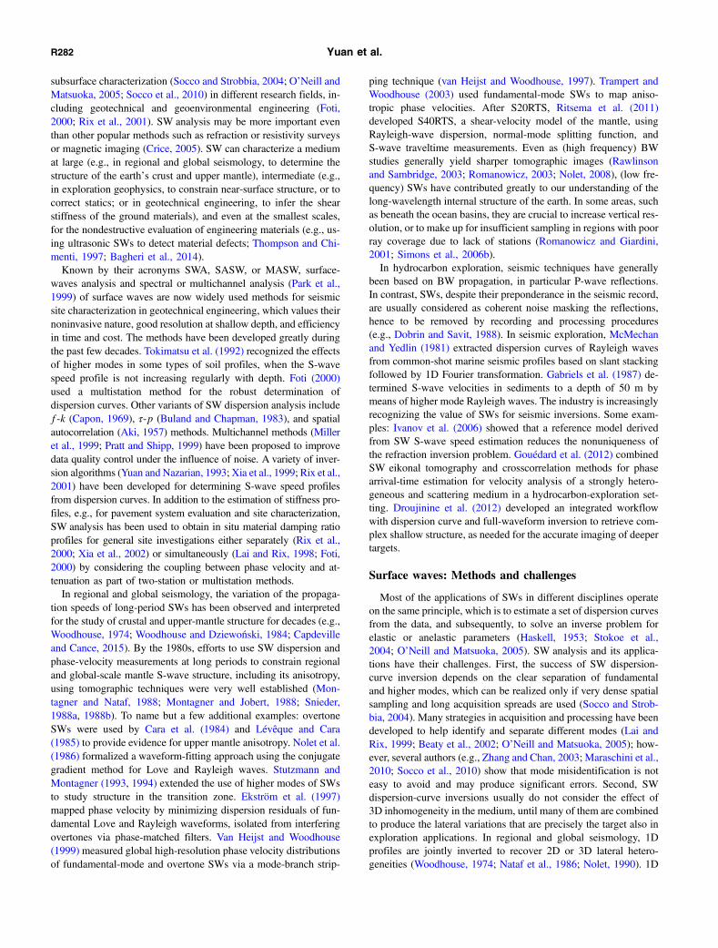
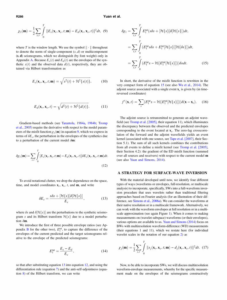
To evaluate the behavior of the various possible measurements inSW inversions, we conduct a numerical experiment in which weconsider four different objective functions. These are: (1) the WDat full resolution, i.e., the “traditional” metric; (2) the WD of seis-mograms progressively reconstructed in a wavelet multiscale fash-ion, i.e., χj of equation 17; (3) the ED at full resolution, i.e., χ1 ofequation 9, or (4) the difference of the envelopes of the seismogramsreconstructed via wavelet multiscale analysis(i.e., χ1j of equation 18).With reference to Figure 1 and again using

SPECFEM2D, we calculate the relevant misfitvalues and plot them as contoured 2D surfacesin the variables VS0 and VS1, the backgroundS-wave speed and the perturbed S-wave speedin the curved layer, respectively. The true valuesare VS0 ¼ 800 m∕s and VS1 ¼ 1000 m∕s andthe calculations range from 600 to 1400 m∕sfor both of them. To evaluate the misfits, weuse one shot gather of a 40 Hz Ricker waveletsource imposed normally to the surface, locatedat 50 m horizontally from the left edge and at0.5 m in depth. We consider the vertical andthe horizontal components of displacement re-corded by a total of 401 receivers spaced 1 mapart and at a depth of 0.5 m below the surface.The total misfit is the sum of the misfits for eachcomponent.The full-resolution (“D12 scale 0”) WD misfit

surface is shown in Figure 2a, and the full-reso-lution ED misfit surface is shown in Figure 2b.The WD misfit displays numerous local minimacaused by the cycle skipping of SWs, which ul-timately will prevent inversions from convergingto the target solution (which lies at the intersec-tion of the white lines) when starting from ahomogeneous model (VS0 ¼ VS1 ¼ 900 m∕s,

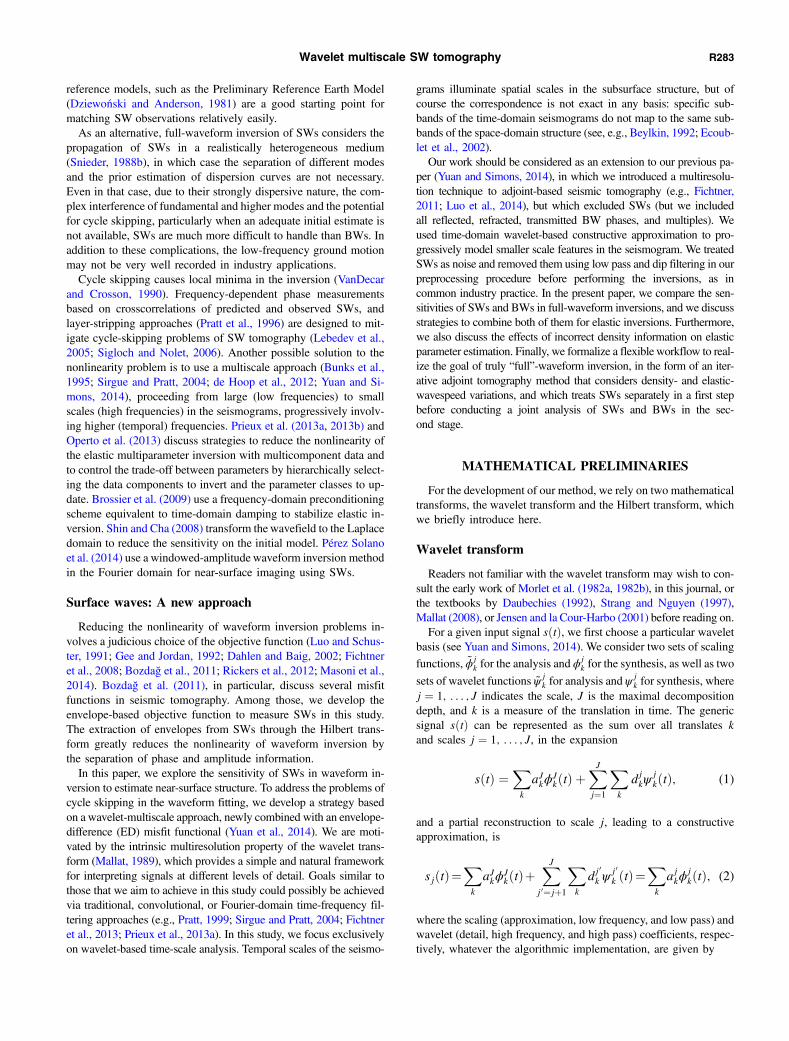
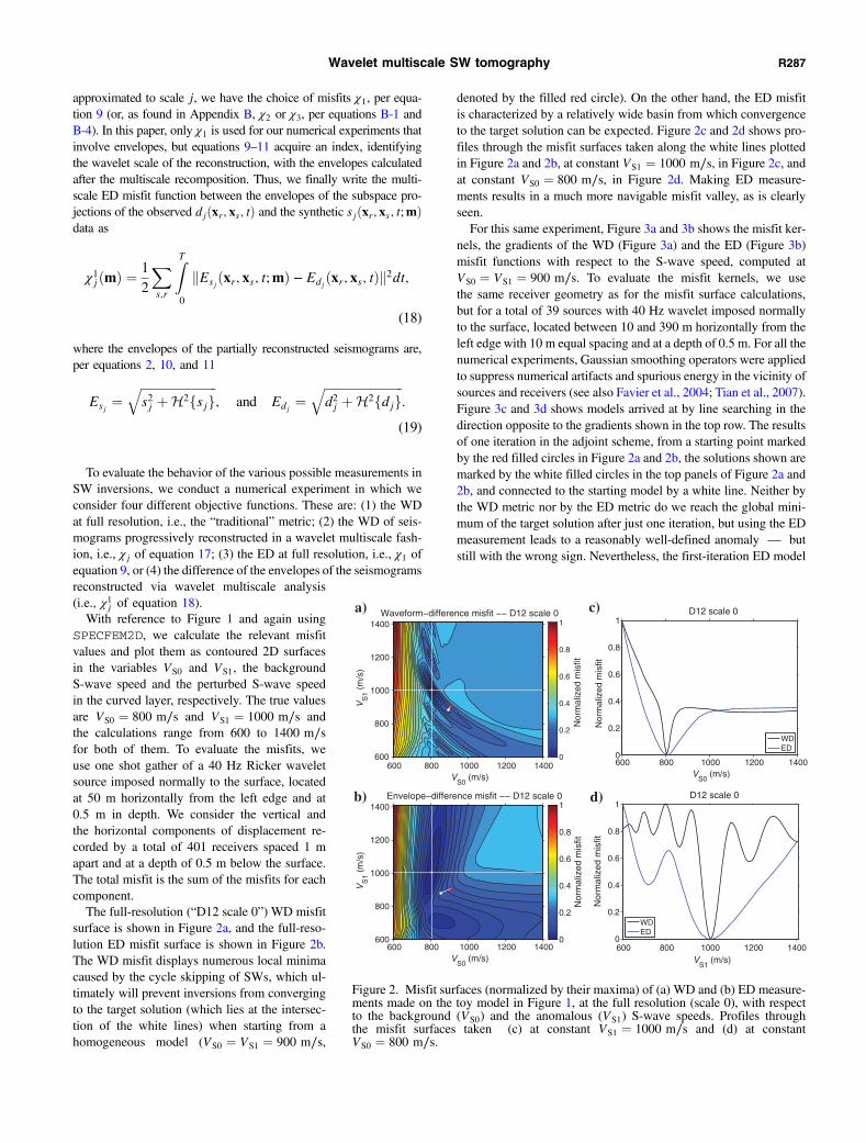
denoted by the filled red circle). On the other hand, the ED misfitis characterized by a relatively wide basin from which convergenceto the target solution can be expected. Figure 2c and 2d shows pro-files through the misfit surfaces taken along the white lines plottedin Figure 2a and 2b, at constant VS1 ¼ 1000 m∕s, in Figure 2c, andat constant VS0 ¼ 800 m∕s, in Figure 2d. Making ED measure-ments results in a much more navigable misfit valley, as is clearlyseen.For this same experiment, Figure 3a and 3b shows the misfit ker-

nels, the gradients of the WD (Figure 3a) and the ED (Figure 3b)misfit functions with respect to the S-wave speed, computed atVS0 ¼ VS1 ¼ 900 m∕s. To evaluate the misfit kernels, we usethe same receiver geometry as for the misfit surface calculations,but for a total of 39 sources with 40 Hz wavelet imposed normallyto the surface, located between 10 and 390 m horizontally from theleft edge with 10 m equal spacing and at a depth of 0.5 m. For all thenumerical experiments, Gaussian smoothing operators were appliedto suppress numerical artifacts and spurious energy in the vicinity ofsources and receivers (see also Favier et al., 2004; Tian et al., 2007).Figure 3c and 3d shows models arrived at by line searching in thedirection opposite to the gradients shown in the top row. The resultsof one iteration in the adjoint scheme, from a starting point markedby the red filled circles in Figure 2a and 2b, the solutions shown aremarked by the white filled circles in the top panels of Figure 2a and2b, and connected to the starting model by a white line. Neither bythe WD metric nor by the ED metric do we reach the global mini-mum of the target solution after just one iteration, but using the EDmeasurement leads to a reasonably well-defined anomaly — butstill with the wrong sign. Nevertheless, the first-iteration ED model

VS0

(m/s)

VS

1 (m

/s)

Waveform−difference misfit −− D12 scale 0

600 800 1000 1200 1400600

800

1000

1200

1400

Nor

mal

ized

mis

fit

0

0.2

0.4

0.6

0.8

1

VS0

(m/s)

VS

1 (m

/s)

Envelope−difference misfit −− D12 scale 0

600 800 1000 1200 1400600

800

1000

1200

1400

Nor

mal

ized

mis

fit

0

0.2

0.4

0.6

0.8

1

600 800 1000 1200 14000

0.2

0.4

0.6

0.8

1

VS0

(m/s)

Nor

mal

ized

mis

fit

D12 scale 0

WDED

600 800 1000 1200 14000

0.2

0.4

0.6

0.8

1

VS1

(m/s)

Nor

mal

ized

mis

fit

D12 scale 0

WDED

a) c)

d)b)

Figure 2. Misfit surfaces (normalized by their maxima) of (a) WD and (b) ED measure-ments made on the toy model in Figure 1, at the full resolution (scale 0), with respectto the background (VS0) and the anomalous (VS1) S-wave speeds. Profiles throughthe misfit surfaces taken (c) at constant VS1 ¼ 1000 m∕s and (d) at constantVS0 ¼ 800 m∕s.


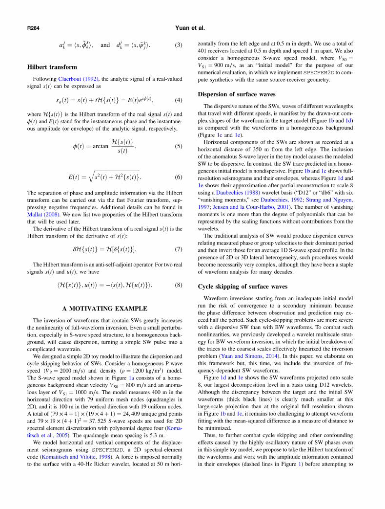
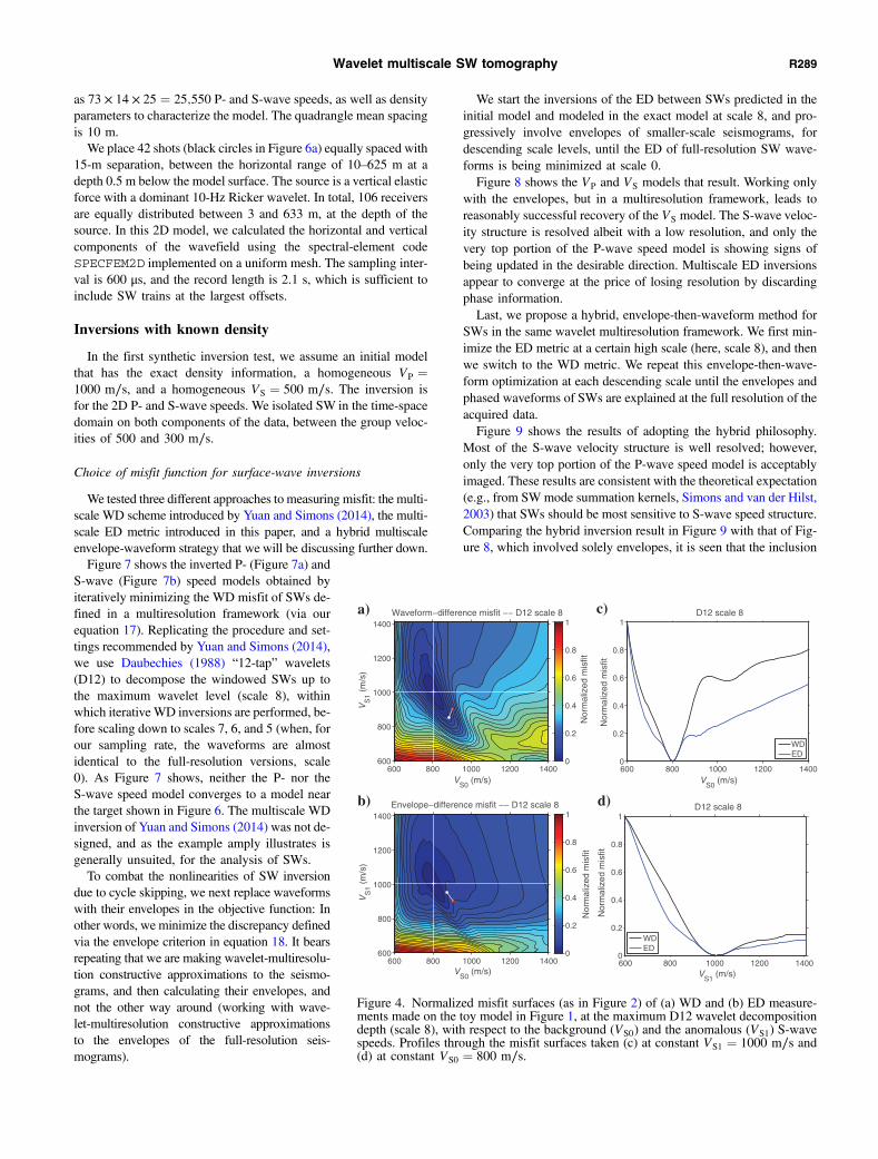
in Figure 3d is a more promising approximation to the target shownin Figure 1a than the WD model shown in Figure 3c.The misfit surface of the WD measured at scale 8 (Figure 4a) is

devoid of the many secondary minima that were present at the fullresolution, at scale 0 (Figure 2a), hinting at an effective remediationof cycle-skipping effects by coarse-scale wavelet approximation ofthe seismograms. Such a finding is consistent with the BW inver-sion experiments of Yuan and Simons (2014), who prove that con-structive approximation by wavelet multiscale analysis reduces thenumber of local minima even when poor initial models are taken asa starting reference. However, unlike with BW waveforms, WDmeasurements made on the coarsest-scale wavelet representationof SW, when used for gradient computations, still insufficiently re-duce the distance between the modeled and the predicted SW wave-forms in the inversion. It is not difficult to encounter examples inwhich convergence to the global optimum remains out of reach dueto the severe nonlinearity of SW inversion caused by cycle skippingof these dispersive and highly oscillatory phases.By ignoring phase variations, ED measurements made at the

coarsest level of a multiscale analysis usefully reduce the non-linearity of SW inversions. Figure 4b shows that the ED misfit

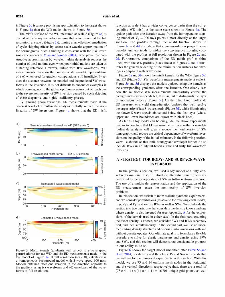
function at scale 8 has a wider convergence basin than the corre-sponding WD misfit at the same scale shown in Figure 4a. Theupdate path after one iteration away from the homogeneous start-ing model of VS ¼ 900 m∕s points almost directly at the targetsolution. The profiles through the misfit function shown inFigure 4c and 4d also show that coarse-resolution projection viawavelet analysis tends to widen the convergence troughs, com-pared with the profiles at full resolution shown in Figure 2c and2d. Furthermore, comparison of the ED misfit profiles (bluelines) with the WD profiles (black lines) in Figures 2 and 4 illus-trates the general widening of the minimization surfaces for enve-lopes compared with waveforms.Figure 5a and 5b shows the misfit kernels for the WD (Figure 5a)

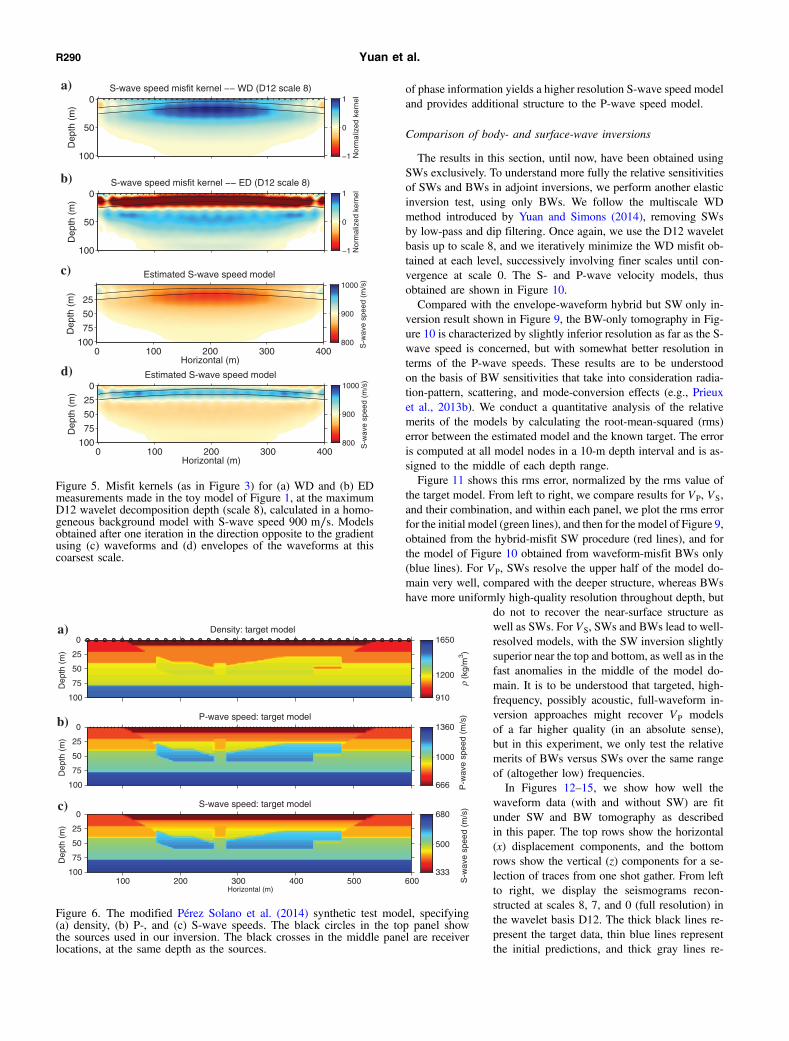
and ED (Figure 5b) SW waveform measurements made at scale 8.Figure 5c and 5d displays the models updated using the kernels asthe corresponding gradients, after one iteration. One clearly seeshow the multiscale WD measurements successfully correct thebackground S-wave speeds but, thus far, fail to distinguish the layerof anomalous velocity (Figure 5c). On the other hand, multiscaleED measurements yield single-iteration updates that well resolvethe target strip of fast S-wave speeds (Figure 5d), while illuminatingthe slower S-wave speeds above and below the fast layer (whoseupper and lower boundaries are drawn with black lines).As far as a toy model can be our guide, the above experiments

lead us to conclude that ED measurements made within a wavelet-multiscale analysis will greatly reduce the nonlinearity of SWtomography, and reduce the critical dependence of waveform inver-sions on the quality of the initial estimates. In the following section,we will elaborate on this initial strategy and develop it further to alsoinclude BWs in an adjoint-based elastic and truly full-waveforminversion.

A STRATEGY FOR BODY- AND SURFACE-WAVEINVERSION

In the previous section, we used a toy model and only con-sidered variations in VS to introduce alternative misfit measuresdedicated to the incorporation of SW in full-waveform inversion.The use of a multiscale representation and the application of theED measurement lessen the nonlinearity of SW inversionproblems.In this section, we switch to more realistic synthetic experiments,

and we consider perturbations (relative to the evolving earth model)in ρ, VS and VP, and we use BWs as well as SWs. We subdivide thesection into two parts: one that considers the density known and onewhere density is also inverted for (see Appendix A for the expres-sions of the kernels used in either case). In the first part, assumingthe exact density is known, we consider SWs and BWs separatelyfirst, and then simultaneously. In the second part, we use an incor-rect starting density structure and discuss elastic inversions with andwithout density updates. Our ultimate goal is to formulate a flexibleprocedure to solve for elastic parameters and density using BWsand SWs, and this section will demonstrate considerable progressin our ability to do so.Figure 6 shows the target model (modified after Pérez Solano

et al., 2014) for density and the elastic P- and S-wave speeds thatwe will use for the numerical experiments in this section. With thismodel, we use 73 and 14 uniform mesh nodes in the horizontaland the vertical directions, respectively; thus, there are a total ofð73 × 4þ 1Þ × ð14 × 4þ 1Þ ¼ 16;701 unique grid points, as well

Dep

th (

m)

S-wave speed misfit kernel −− WD (D12 scale 0)0

50

100 Nor

mal

ized

ker

nel

−1

0

1

Dep

th (

m)

S-wave speed misfit kernel −− ED (D12 scale 0)0

50

100 Nor

mal

ized

ker

nel

−1

0

1

Horizontal (m)

Dep

th (

m)

Estimated S-wave speed model

0 100 200 300 400

0

25

50

75

100 S-w

ave

spee

d (m

/s)

800

900

1000

Horizontal (m)

Dep

th (

m)


0 100 200 300 400

0

25

50

75

100 S-w

ave

spee

d (m

/s)

800

900

1000

a)

b)

c)

d)

Figure 3. Misfit kernels (gradients with respect to S-wave speedperturbations) for (a) WD and (b) ED measurements made in thetoy model of Figure 1a, at full resolution (scale 0), calculated ina homogeneous background model with S-wave speed 900 m∕s.Models obtained after one iteration in the direction opposite tothe gradient using (c) waveforms and (d) envelopes of the wave-forms at full resolution.

R288 Yuan et al.

as 73 × 14 × 25 ¼ 25;550 P- and S-wave speeds, as well as densityparameters to characterize the model. The quadrangle mean spacingis 10 m.We place 42 shots (black circles in Figure 6a) equally spaced with

15-m separation, between the horizontal range of 10–625 m at adepth 0.5 m below the model surface. The source is a vertical elasticforce with a dominant 10-Hz Ricker wavelet. In total, 106 receiversare equally distributed between 3 and 633 m, at the depth of thesource. In this 2D model, we calculated the horizontal and verticalcomponents of the wavefield using the spectral-element codeSPECFEM2D implemented on a uniform mesh. The sampling inter-val is 600 μs, and the record length is 2.1 s, which is sufficient toinclude SW trains at the largest offsets.

Inversions with known density

In the first synthetic inversion test, we assume an initial modelthat has the exact density information, a homogeneous VP ¼1000 m∕s, and a homogeneous VS ¼ 500 m∕s. The inversion isfor the 2D P- and S-wave speeds. We isolated SW in the time-spacedomain on both components of the data, between the group veloc-ities of 500 and 300 m∕s.

Choice of misfit function for surface-wave inversions

We tested three different approaches to measuring misfit: the multi-scale WD scheme introduced by Yuan and Simons (2014), the multi-scale ED metric introduced in this paper, and a hybrid multiscaleenvelope-waveform strategy that we will be discussing further down.Figure 7 shows the inverted P- (Figure 7a) and

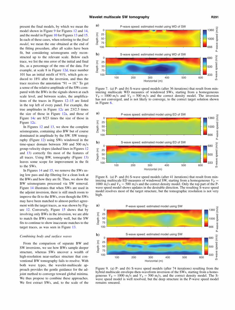
S-wave (Figure 7b) speed models obtained byiteratively minimizing the WD misfit of SWs de-fined in a multiresolution framework (via ourequation 17). Replicating the procedure and set-tings recommended by Yuan and Simons (2014),we use Daubechies (1988) “12-tap” wavelets(D12) to decompose the windowed SWs up tothe maximum wavelet level (scale 8), withinwhich iterativeWD inversions are performed, be-fore scaling down to scales 7, 6, and 5 (when, forour sampling rate, the waveforms are almostidentical to the full-resolution versions, scale0). As Figure 7 shows, neither the P- nor theS-wave speed model converges to a model nearthe target shown in Figure 6. The multiscale WDinversion of Yuan and Simons (2014) was not de-signed, and as the example amply illustrates isgenerally unsuited, for the analysis of SWs.To combat the nonlinearities of SW inversion

due to cycle skipping, we next replace waveformswith their envelopes in the objective function: Inother words, we minimize the discrepancy definedvia the envelope criterion in equation 18. It bearsrepeating that we are making wavelet-multiresolu-tion constructive approximations to the seismo-grams, and then calculating their envelopes, andnot the other way around (working with wave-let-multiresolution constructive approximationsto the envelopes of the full-resolution seis-mograms).

We start the inversions of the ED between SWs predicted in theinitial model and modeled in the exact model at scale 8, and pro-gressively involve envelopes of smaller-scale seismograms, fordescending scale levels, until the ED of full-resolution SW wave-forms is being minimized at scale 0.Figure 8 shows the VP and VS models that result. Working only

with the envelopes, but in a multiresolution framework, leads toreasonably successful recovery of the VS model. The S-wave veloc-ity structure is resolved albeit with a low resolution, and only thevery top portion of the P-wave speed model is showing signs ofbeing updated in the desirable direction. Multiscale ED inversionsappear to converge at the price of losing resolution by discardingphase information.Last, we propose a hybrid, envelope-then-waveform method for

SWs in the same wavelet multiresolution framework. We first min-imize the ED metric at a certain high scale (here, scale 8), and thenwe switch to the WD metric. We repeat this envelope-then-wave-form optimization at each descending scale until the envelopes andphased waveforms of SWs are explained at the full resolution of theacquired data.Figure 9 shows the results of adopting the hybrid philosophy.

Most of the S-wave velocity structure is well resolved; however,only the very top portion of the P-wave speed model is acceptablyimaged. These results are consistent with the theoretical expectation(e.g., from SWmode summation kernels, Simons and van der Hilst,2003) that SWs should be most sensitive to S-wave speed structure.Comparing the hybrid inversion result in Figure 9 with that of Fig-ure 8, which involved solely envelopes, it is seen that the inclusion

VS0

(m/s)

VS

1 (m

/s)

Waveform−difference misfit −− D12 scale 8

600 800 1000 1200 1400600

800

1000

1200

1400

Nor

mal

ized

mis

fit

0

0.2

0.4

0.6

0.8

1

VS0

(m/s)

VS

1 (m

/s)

Envelope−difference misfit −− D12 scale 8

600 800 1000 1200 1400600

800

1000

1200

1400

Nor

mal

ized

mis

fit

0

0.2

0.4

0.6

0.8

1

600 800 1000 1200 14000

0.2

0.4

0.6

0.8

1

VS0

(m/s)

Nor

mal

ized

mis

fitD12 scale 8

WDED

600 800 1000 1200 14000

0.2

0.4

0.6

0.8

1

VS1

(m/s)

Nor

mal

ized

mis

fit

D12 scale 8

WDED

a) c)

b) d)

Figure 4. Normalized misfit surfaces (as in Figure 2) of (a) WD and (b) ED measure-ments made on the toy model in Figure 1, at the maximum D12 wavelet decompositiondepth (scale 8), with respect to the background (VS0) and the anomalous (VS1) S-wavespeeds. Profiles through the misfit surfaces taken (c) at constant VS1 ¼ 1000 m∕s and(d) at constant VS0 ¼ 800 m∕s.


of phase information yields a higher resolution S-wave speed modeland provides additional structure to the P-wave speed model.

Comparison of body- and surface-wave inversions

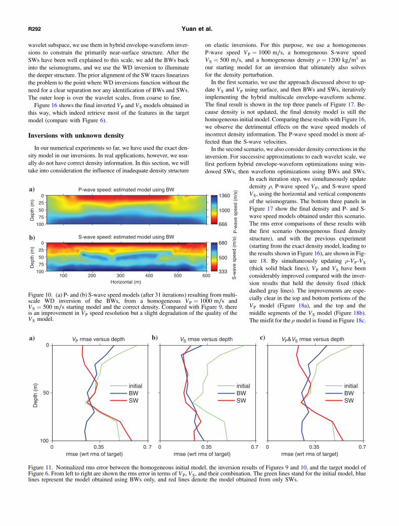
The results in this section, until now, have been obtained usingSWs exclusively. To understand more fully the relative sensitivitiesof SWs and BWs in adjoint inversions, we perform another elasticinversion test, using only BWs. We follow the multiscale WDmethod introduced by Yuan and Simons (2014), removing SWsby low-pass and dip filtering. Once again, we use the D12 waveletbasis up to scale 8, and we iteratively minimize the WD misfit ob-tained at each level, successively involving finer scales until con-vergence at scale 0. The S- and P-wave velocity models, thusobtained are shown in Figure 10.Compared with the envelope-waveform hybrid but SW only in-

version result shown in Figure 9, the BW-only tomography in Fig-ure 10 is characterized by slightly inferior resolution as far as the S-wave speed is concerned, but with somewhat better resolution interms of the P-wave speeds. These results are to be understoodon the basis of BW sensitivities that take into consideration radia-tion-pattern, scattering, and mode-conversion effects (e.g., Prieuxet al., 2013b). We conduct a quantitative analysis of the relativemerits of the models by calculating the root-mean-squared (rms)error between the estimated model and the known target. The erroris computed at all model nodes in a 10-m depth interval and is as-signed to the middle of each depth range.Figure 11 shows this rms error, normalized by the rms value of

the target model. From left to right, we compare results for VP, VS,and their combination, and within each panel, we plot the rms errorfor the initial model (green lines), and then for the model of Figure 9,obtained from the hybrid-misfit SW procedure (red lines), and forthe model of Figure 10 obtained from waveform-misfit BWs only(blue lines). For VP, SWs resolve the upper half of the model do-main very well, compared with the deeper structure, whereas BWshave more uniformly high-quality resolution throughout depth, but

do not to recover the near-surface structure aswell as SWs. For VS, SWs and BWs lead to well-resolved models, with the SW inversion slightlysuperior near the top and bottom, as well as in thefast anomalies in the middle of the model do-main. It is to be understood that targeted, high-frequency, possibly acoustic, full-waveform in-version approaches might recover VP modelsof a far higher quality (in an absolute sense),but in this experiment, we only test the relativemerits of BWs versus SWs over the same rangeof (altogether low) frequencies.In Figures 12–15, we show how well the

waveform data (with and without SW) are fitunder SW and BW tomography as describedin this paper. The top rows show the horizontal(x) displacement components, and the bottomrows show the vertical (z) components for a se-lection of traces from one shot gather. From leftto right, we display the seismograms recon-structed at scales 8, 7, and 0 (full resolution) inthe wavelet basis D12. The thick black lines re-present the target data, thin blue lines representthe initial predictions, and thick gray lines re-

Dep

th (

m)

S-wave speed misfit kernel −− WD (D12 scale 8)0

50

100 Nor

mal

ized

ker

nel

−1

0

1

Dep

th (

m)

S-wave speed misfit kernel −− ED (D12 scale 8)0

50

100 Nor

mal

ized

ker

nel

−1

0

1

Horizontal (m)

Dep

th (

m)


0 100 200 300 400

25

50

75

100 S-w

ave

spee

d (m

/s)

800

900

1000

Horizontal (m)

Dep

th (

m)


0 100 200 300 400

0

25

50

75

100 S-w

ave

spee

d (m

/s)

800

900

1000

a)

b)

c)

d)

Figure 5. Misfit kernels (as in Figure 3) for (a) WD and (b) EDmeasurements made in the toy model of Figure 1, at the maximumD12 wavelet decomposition depth (scale 8), calculated in a homo-geneous background model with S-wave speed 900 m∕s. Modelsobtained after one iteration in the direction opposite to the gradientusing (c) waveforms and (d) envelopes of the waveforms at thiscoarsest scale.

Dep

th (

m)

Density: target model0

25

50

75

100

ρ (k

g/m

3 )

910

1200

1650

Dep

th (

m)

P-wave speed: target model0

25

50

75

100 P-w

ave

spee

d (m

/s)

666

1000

1360

Horizontal (m)

Dep

th (

m)

S-wave speed: target model

100 200 300 400 500 600

0

25

50

75

100

S-w

ave

spee

d (m

/s)

333

500

680

a)

b)

c)

Figure 6. The modified Pérez Solano et al. (2014) synthetic test model, specifying(a) density, (b) P-, and (c) S-wave speeds. The black circles in the top panel showthe sources used in our inversion. The black crosses in the middle panel are receiverlocations, at the same depth as the sources.

R290 Yuan et al.

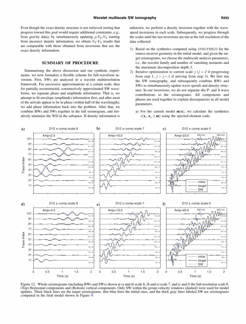
present the final models, by which we mean themodel shown in Figure 9 for Figures 12 and 14,and the model in Figure 10 for Figures 13 and 15.In each of these cases, when referring to the finalmodel, we mean the one obtained at the end ofthe fitting procedure, after all scales have beenfit, but considering seismograms only recon-structed up to the relevant scale. Below eachtrace, we list the rms error of the initial and finalfits, as a percentage of the rms of the data. Forexample, at scale 8 in Figure 12d, trace number101 has an initial misfit of 91%, which gets re-duced to 18% after the inversion, and thus thetrace receives the annotation “91 → 18.” To geta sense of the relative amplitude of the SWs com-pared with the BWs in the signals shown at eachscale level, and between scales, the amplifica-tions of the traces in Figures 12–15 are listedin the top left of every panel. For example, thetrue amplitudes in Figure 12c are 23/2.5 timesthe size of those in Figure 12a, and those ofFigure 14c are 8/23 times the size of those inFigure 12c.In Figures 12 and 13, we show the complete

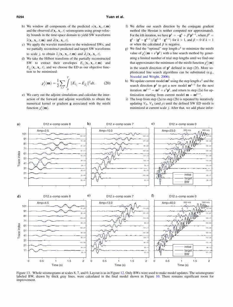
seismograms, containing also BW but of coursedominated in amplitude by the SW. SW tomog-raphy (Figure 12) using SWs windowed in thetime-space domain between 300 and 500 m∕sgroup-velocity slopes (dashed lines in Figures 12and 13) correctly fits most of the features ofall traces. Using BW, tomography (Figure 13)leaves some scope for improvement in the fitto the SWs.In Figures 14 and 15, we remove the SWs us-

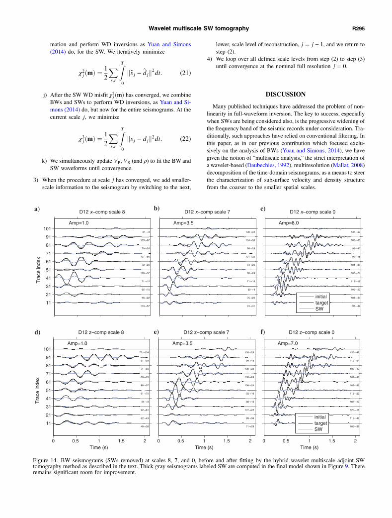
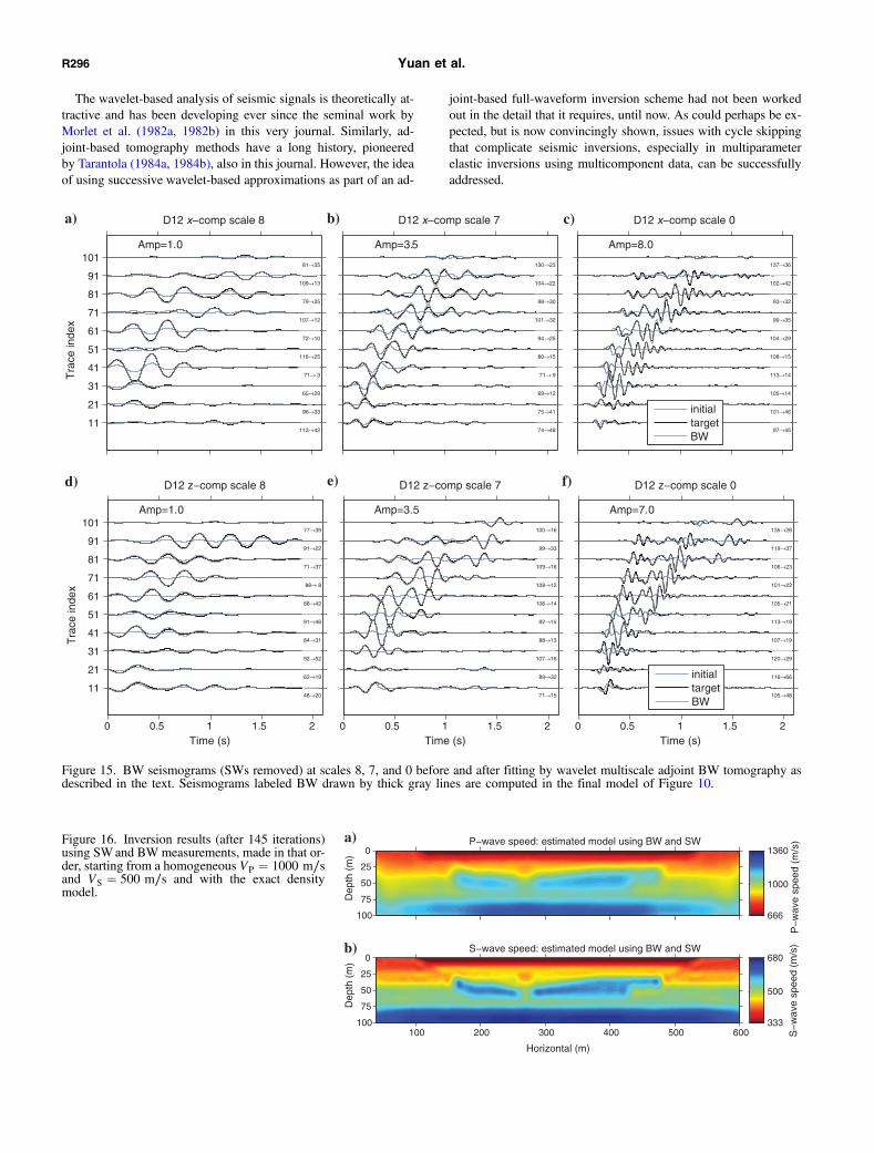
ing low pass and dip filtering for a clean look atthe BWs and how they are fit. Thus, we show theBW seismograms processed via SW removal.Figure 14 illustrates that when SWs are used inthe adjoint inversion, there is still much room toimprove the fit to the BWs, even though the SWsmay have been matched to almost-perfect agree-ment with the target traces, as was shown by Fig-ure 12. Conversely, Figure 15 shows that byinvolving only BWs in the inversion, we are ableto match the BWs reasonably well, but the SWfits to continue to show inaccurate matches to thetarget traces, as was seen in Figure 13.

Combining body and surface waves

From the comparison of separate BW andSW inversions, we see how BWs sample deeperstructure, whereas SWs uncover a wealth ofhigh-resolution near-surface structure that con-ventional BW tomography fails to resolve. Withboth wave types, the wavelet-multiscale ap-proach provides the gentle guidance for the ad-joint method to converge toward global minima.We thus propose to combine these approaches.We first extract SWs, and, to the scale of the

Dep

th (

m)

P-wave speed: estimated model using WD of SW0

25

50

75

100

P-w

ave

spee

d (m

/s)

666

1000

1360

Horizontal (m)

Dep

th (

m)

S-wave speed: estimated model using WD of SW

100 200 300 400 500 600

0

25

50

75

100

S-w

ave

spee

d (m

/s)

333

500

680

a)

b)

Figure 7. (a) P- and (b) S-wave speed models (after 36 iterations) that result from min-imizing multiscale WD measures of windowed SWs, starting from a homogeneousVP ¼ 1000 m∕s and VS ¼ 500 m∕s and the correct density model. The inversionhas not converged, and is not likely to converge, to the correct target solution shownin Figure 6.

Dep

th (

m)

P-wave speed: estimated model using ED of SW0

25

50

75

100

P-w

ave

spee

d (m

/s)

666

1000

1360

Horizontal (m)

Dep

th (

m)

S-wave speed: estimated model using ED of SW

100 200 300 400 500 600

0

25

50

75

100

S-w

ave

spee

d (m

/s)

333

500

680

a)

b)

Figure 8. (a) P- and (b) S-wave speed models (after 41 iterations) that result from min-imizing multiscale ED measures of windowed SW, starting from a homogeneous VP ¼1000 m∕s and VS ¼ 500 m∕s and the correct density model. Only the top part of the P-wave speed model shows updates in the desirable direction. The resulting S-wave speedmodel resolves most of the target structure, but the tomographic resolution is not veryhigh.

Dep

th (

m)

P-wave speed: estimated model using SW0

25

50

75

100

P-w

ave

spee

d (m

/s)

666

1000

1360

Horizontal (m)

Dep

th (

m)

S-wave speed: estimated model using SW

100 200 300 400 500 600

0

25

50

75

100

S-w

ave

spee

d (m

/s)

333

500

680

a)

b)

Figure 9. (a) P- and (b) S-wave speed models (after 74 iterations) resulting from thehybrid multiscale envelope-then-waveform inversion of the SWs, starting from a homo-geneous VP ¼ 1000 m∕s and VS ¼ 500 m∕s, and the correct density model. The S-wave speed model is well resolved, but the deep structure in the P-wave speed modelremains smeared.


wavelet subspace, we use them in hybrid envelope-waveform inver-sions to constrain the primarily near-surface structure. After theSWs have been well explained to this scale, we add the BWs backinto the seismograms, and we use the WD inversion to illuminatethe deeper structure. The prior alignment of the SW traces linearizesthe problem to the point where WD inversions function without theneed for a clear separation nor any identification of BWs and SWs.The outer loop is over the wavelet scales, from coarse to fine.Figure 16 shows the final inverted VP and VS models obtained in

this way, which indeed retrieve most of the features in the targetmodel (compare with Figure 6).

Inversions with unknown density

In our numerical experiments so far, we have used the exact den-sity model in our inversions. In real applications, however, we usu-ally do not have correct density information. In this section, we willtake into consideration the influence of inadequate density structure

on elastic inversions. For this purpose, we use a homogeneousP-wave speed VP ¼ 1000 m∕s, a homogeneous S-wave speedVS ¼ 500 m∕s, and a homogeneous density ρ ¼ 1200 kg∕m3 asour starting model for an inversion that ultimately also solvesfor the density perturbation.In the first scenario, we use the approach discussed above to up-

date VS and VP using surface, and then BWs and SWs, iterativelyimplementing the hybrid multiscale envelope-waveform scheme.The final result is shown in the top three panels of Figure 17. Be-cause density is not updated, the final density model is still thehomogeneous initial model. Comparing these results with Figure 16,we observe the detrimental effects on the wave speed models ofincorrect density information. The P-wave speed model is more af-fected than the S-wave velocities.In the second scenario, we also consider density corrections in the

inversion. For successive approximations to each wavelet scale, wefirst perform hybrid envelope-waveform optimizations using win-dowed SWs, then waveform optimizations using BWs and SWs.

In each iteration step, we simultaneously updatedensity ρ, P-wave speed VP, and S-wave speedVS, using the horizontal and vertical componentsof the seismograms. The bottom three panels inFigure 17 show the final density and P- and S-wave speed models obtained under this scenario.The rms error comparisons of these results withthe first scenario (homogeneous fixed densitystructure), and with the previous experiment(starting from the exact density model, leading tothe results shown in Figure 16), are shown in Fig-ure 18. By simultaneously updating ρ-VP-VS

(thick solid black lines), VP and VS have beenconsiderably improved compared with the inver-sion results that held the density fixed (thickdashed gray lines). The improvements are espe-cially clear in the top and bottom portions of theVP model (Figure 18a), and the top and themiddle segments of the VS model (Figure 18b).The misfit for the ρmodel is found in Figure 18c.

Dep

th (

m)

P-wave speed: estimated model using BW0

25

50

75

100

P-w

ave

spee

d (m

/s)

666

1000

1360

Horizontal (m)

Dep

th (

m)

S-wave speed: estimated model using BW

100 200 300 400 500 600

0

25

50

75

100

S-w

ave

spee

d (m

/s)

333

500

680

a)

b)

Figure 10. (a) P- and (b) S-wave speed models (after 31 iterations) resulting from multi-scale WD inversion of the BWs, from a homogeneous VP ¼ 1000 m∕s andVS ¼ 500 m∕s starting model and the correct density. Compared with Figure 9, thereis an improvement in VP speed resolution but a slight degradation of the quality of theVS model.

0 0.35 0. 7

0

50

100

rmse (wrt rms of target)

Dep

th (

m)

VP rmse versus depth

initialBWSW

0 0.35 0.7


VS rmse versus depth

initialBWSW

0 0.35 0.7


VP&VS rmse versus depth

initialBWSW

a) b) c)

Figure 11. Normalized rms error between the homogeneous initial model, the inversion results of Figures 9 and 10, and the target model ofFigure 6. From left to right are shown the rms error in terms of VP, VS, and their combination. The green lines stand for the initial model, bluelines represent the model obtained using BWs only, and red lines denote the model obtained from only SWs.

R292 Yuan et al.

Even though the exact density structure is not retrieved (noting thatprogress toward this goal would require additional constraints, e.g.,from gravity data), by simultaneously updating ρ-VP-VS startingfrom incorrect density information, we obtain VP-VS results thatare comparable with those obtained from inversions that use theexact density information.

SUMMARY OF PROCEDURE

Summarizing the above discussion and our synthetic experi-ments, we now formalize a flexible scheme for full-waveform in-version. First, SWs are analyzed in a wavelet multiresolutionframework. For successive approximations at a certain scale, thusfor partially reconstructed, constructively approximated SW wave-forms, we separate phase and amplitude information. That is, weattempt to fit envelope (amplitude) information first, and after mostof the arrivals appear to be in phase (within half of the wavelength),we add phase information back into the problem. After that, wecombine BWs and SWs together in the full seismogram, and iter-atively minimize the WD in the subspace. If density information is

unknown, we perform a density inversion together with the wave-speed inversions in each scale. Subsequently, we progress throughthe scales until the last inversions are run at the full resolution of thedata collected.

1) Based on the synthetics computed using SPECFEM2D for thesource-receiver geometry in the initial model, and given the tar-get seismograms, we choose the multiscale analysis parameters,i.e., the wavelet family and number of vanishing moments andthe maximum decomposition depth J.

2) Iterative optimization to current scale j (j ¼ J if progressingfrom step 1, j ¼ j − 1 if arriving from step 3). We first runthe SW tomography, and subsequently combine BWs andSWs to simultaneously update wave speeds and density struc-ture. In our inversions, we do not separate the P- and S-wavecontributions to the seismograms. All components andphases are used together to explain discrepancies in all modelparameters.

a) For the current model mðxÞ, we calculate the syntheticssðxr; xs; t;mÞ using the spectral-element code.

11

21

31

41

51

61

71

81

91

101

65→43

33→21

46→ 9

59→ 5

59→25

97→49

87→32

81→16

70→105

102→88

Amp=2.5

Tra

ce in

dex

D12 x−comp scale 8

50→ 6

102→ 8

29→ 4

76→ 4

102→ 7

121→10

102→17

89→33

127→30

103→28

Amp=10.0


500 m/s 300 m/s

96→ 6

83→10

113→ 9

110→ 8

114→ 9

101→14

109→19

109→21

106→22

114→25

Amp=23.0


initialtargetSW

0 0.5 1 1.5 2

11

21

31

41

51

61

71

81

91

101

29→10

44→20

170→31

59→25

68→35

132→45

68→25

129→83

98→40

91→18

Amp=4.5

Time (s)

Tra

ce in

dex

D12 z−comp scale 8

0 0.5 1 1.5 2

22→ 5

59→ 5

99→ 5

134→ 7

144→17

101→13

99→13

113→15

101→15

114→20

Amp=13.0

Time (s)


0 0.5 1 1.5 2

500 m/s 300 m/s

101→ 5

88→ 4

115→ 4

112→ 6

109→ 7

110→12

104→15

100→20

112→24

116→26

Amp=40.0

Time (s)


initialtargetSW

a) b) c)

d) e) f)

Figure 12. Whole seismograms (including BWs and SWs) shown at (a and d) scale 8, (b and e) scale 7, and (c and f) the full-resolution scale 0.(Top) Horizontal components and (Bottom) vertical components. Only SW within the group-velocity windows (dashed) were used for modelupdates. Thick black lines are the target seismograms, thin blue lines the initial ones, and the thick gray lines labeled SW are seismogramscomputed in the final model shown in Figure 9.


b) We window all components of the predicted sðxr; xs; t;mÞand the observed dðxr; xs; tÞ seismograms using group-veloc-ity bounds in the time-space domain to yield SW waveforms

sðxr; xs; t;mÞ and dðxr; xs; tÞ.c) We apply the wavelet transform to the windowed SWs, and

we partially reconstruct predicted and target SW waveforms

to scale j, to obtain sjðxr; xs; t;mÞ and djðxr; xs; tÞ.d) We take the Hilbert transform of the partially reconstructed

SW to extract their envelopes Esjðxr; xs; t;mÞ andEdj

ðxr; xs; tÞ, and we choose the ED as our objective func-tion to be minimized:

χ1jðmÞ ¼ 1

2

Xs;r

ZT

0

kEsj − Edjk2dt: (20)

e) We carry out the adjoint simulations and calculate the inter-action of the forward and adjoint wavefields to obtain thenumerical kernel or gradient g associated with the misfitfunction χ1j ðmÞ.

f) We define our search direction by the conjugate gradientmethod (the Hessian is neither computed nor approximated).For the kth iteration, we have pk ¼ −gk þ βkpk−1, where βk ¼gk · ðgk − gk−1Þ∕ðgk−1 · gk−1Þ for k > 1, and β ¼ 0 if k ¼ 1

or when the calculated β is negative.g) We find the “optimal” step length νk to minimize the misfit

value of χ1jðmþ νkpkÞ with a line search method by gener-ating a limited number of trial step lengths until we find onethat approximates the minimum of the misfit function χ1j ðmÞin the search direction of pk defined in step (2f). More so-phisticated line search algorithms can be substituted (e.g.,Nocedal and Wright, 2006).

h) We update current modelmk using the step length νk and thesearch direction pk to get a new model mkþ1 for the nextiteration: mkþ1 ¼ mk þ νkpk, and return to step (2a) for op-timization starting from current model m ¼ mkþ1.

i) The loop from step (2a) to step (2h) is repeated by iterativelyupdating VP, VS (and ρ) until the defined SW ED misfit isminimized at current scale j. After that, we add phase infor-

11

21

31

41

51

61

71

81

91

101

65→37

33→55

46→21

59→ 7

59→13

97→15

87→17

81→27

70→35

102→37

Amp=2.5

Tra

ce in

dex


50→ 8

102→46

29→10

76→ 5

102→ 8

121→ 6

102→23

89→22

127→23

103→16

Amp=10.0


500 m/s 300 m/s

96→13

83→17

113→12

110→14

114→33

101→48

109→49

109→54

106→65

114→45

Amp=23.0


initialtargetBW

0 0.5 1 1.5 2

11

21

31

41

51

61

71

81

91

101

29→ 9

44→14

170→56

59→17

68→33

132→47

68→16

129→34

98→24

91→22

Amp=4.5

Time (s)

Tra

ce in

dex


0 0.5 1 1.5 2

22→ 8

59→ 4

99→15

134→ 7

144→28

101→ 7

99→ 9

113→16

101→16

114→23

Amp=13.0

Time (s)


0 0.5 1 1.5 2

500 m/s 300 m/s

101→19

88→13

115→16

112→25

109→40

110→55

104→63

100→70

112→67

116→49

Amp=40.0

Time (s)


initialtargetBW

a) b) c)

d) e) f)

Figure 13. Whole seismograms at scales 8, 7, and 0. Layout is as in Figure 12. Only BWs were used to make model updates. The seismogramslabeled BW, drawn by thick gray lines, were calculated in the final model shown in Figure 10. There remains significant room forimprovement.

R294 Yuan et al.

mation and perform WD inversions as Yuan and Simons(2014) do, for the SW. We iteratively minimize

χ2jðmÞ ¼ 1

2

Xs;r

ZT

0

ksj − djk2dt: (21)

j) After the SW WD misfit χ2jðmÞ has converged, we combineBWs and SWs to perform WD inversions, as Yuan and Si-mons (2014) do, but now for the entire seismograms. At thecurrent scale j, we minimize

χ3jðmÞ ¼ 1

2

Xs;r

ZT

0

ksj − djk2dt: (22)

k) We simultaneously update VP, VS (and ρ) to fit the BW andSW waveforms until convergence.

3) When the procedure at scale j has converged, we add smaller-scale information to the seismogram by switching to the next,

lower, scale level of reconstruction, j ¼ j − 1, and we return tostep (2).

4) We loop over all defined scale levels from step (2) to step (3)until convergence at the nominal full resolution j ¼ 0.

DISCUSSION

Many published techniques have addressed the problem of non-linearity in full-waveform inversion. The key to success, especiallywhen SWs are being considered also, is the progressive widening ofthe frequency band of the seismic records under consideration. Tra-ditionally, such approaches have relied on conventional filtering. Inthis paper, as in our previous contribution which focused exclu-sively on the analysis of BWs (Yuan and Simons, 2014), we havegiven the notion of “multiscale analysis,” the strict interpretation ofa wavelet-based (Daubechies, 1992), multiresolution (Mallat, 2008)decomposition of the time-domain seismograms, as a means to steerthe characterization of subsurface velocity and density structurefrom the coarser to the smaller spatial scales.

11

21

31

41

51

61

71

81

91

101

113→57

96→22

65→15

71→10

116→37

72→20

107→56

79→26

109→67

81→ 8

Amp=1.0

Tra

ce in

dex


74→31

75→20

69→ 9

71→15

80→24

94→26

101→22

98→29

104→36

130→34

Amp=3.5


97→42

101→44

105→23

113→16

108→24

104→35

99→48

93→43

102→60

137→57

Amp=8.0


initialtargetSW

0 0.5 1 1.5 2

11

21

31

41

51

61

71

81

91

101

48→38

62→43

92→61

84→ 8

91→70

88→37

88→29

71→60

91→39

77→134

Amp=1.0

Time (s)

Tra

ce in

dex


0 0.5 1 1.5 2

71→29

89→36

107→22

88→14

92→16

106→24

108→24

109→32

99→43

100→29

Amp=3.5

Time (s)


0 0.5 1 1.5 2

105→36

116→49

120→18

107→17

113→22

105→32

101→41

106→47

119→64

135→49

Amp=7.0

Time (s)


initialtargetSW

a) b) c)

d) e) f)

Figure 14. BW seismograms (SWs removed) at scales 8, 7, and 0, before and after fitting by the hybrid wavelet multiscale adjoint SWtomography method as described in the text. Thick gray seismograms labeled SW are computed in the final model shown in Figure 9. Thereremains significant room for improvement.


The wavelet-based analysis of seismic signals is theoretically at-tractive and has been developing ever since the seminal work byMorlet et al. (1982a, 1982b) in this very journal. Similarly, ad-joint-based tomography methods have a long history, pioneeredby Tarantola (1984a, 1984b), also in this journal. However, the ideaof using successive wavelet-based approximations as part of an ad-

joint-based full-waveform inversion scheme had not been workedout in the detail that it requires, until now. As could perhaps be ex-pected, but is now convincingly shown, issues with cycle skippingthat complicate seismic inversions, especially in multiparameterelastic inversions using multicomponent data, can be successfullyaddressed.

11

21

31

41

51

61

71

81

91

101

113→42

96→33

65→29

71→ 3

116→25

72→10

107→12

79→25

109→13

81→35

Amp=1.0

Tra

ce in

dex


74→48

75→41

69→12

71→ 9

80→15

94→25

101→32

98→30

104→22

130→23

Amp=3.5


97→45

101→46

105→14

113→14

108→15

104→29

99→35

93→32

102→42

137→36

Amp=8.0


initialtargetBW

0 0.5 1 1.5 2

11

21

31

41

51

61

71

81

91

101

48→20

62→19

92→52

84→31

91→46

88→42

88→ 8

71→37

91→22

77→39

Amp=1.0

Time (s)

Tra

ce in

dex


0 0.5 1 1.5 2

71→15

89→32

107→16

88→13

92→15

106→14

108→12

109→16

99→33

100→16

Amp=3.5

Time (s)


0 0.5 1 1.5 2

105→48

116→66

120→29

107→19

113→19

105→21

101→22

106→23

119→37

135→28

Amp=7.0

Time (s)


initialtargetBW

a) b) c)

d) e) f)

Figure 15. BW seismograms (SWs removed) at scales 8, 7, and 0 before and after fitting by wavelet multiscale adjoint BW tomography asdescribed in the text. Seismograms labeled BW drawn by thick gray lines are computed in the final model of Figure 10.

Dep

th (

m)

P−wave speed: estimated model using BW and SW0

25

50

75

100

P−

wav

e sp

eed

(m/s

)

666

1000

1360

Horizontal (m)

Dep

th (

m)

S−wave speed: estimated model using BW and SW

100 200 300 400 500 600

0

25

50

75

100

S−

wav

e sp

eed

(m/s

)

333

500

680

a)

b)

Figure 16. Inversion results (after 145 iterations)using SWand BW measurements, made in that or-der, starting from a homogeneous VP ¼ 1000 m∕sand VS ¼ 500 m∕s and with the exact densitymodel.

R296 Yuan et al.

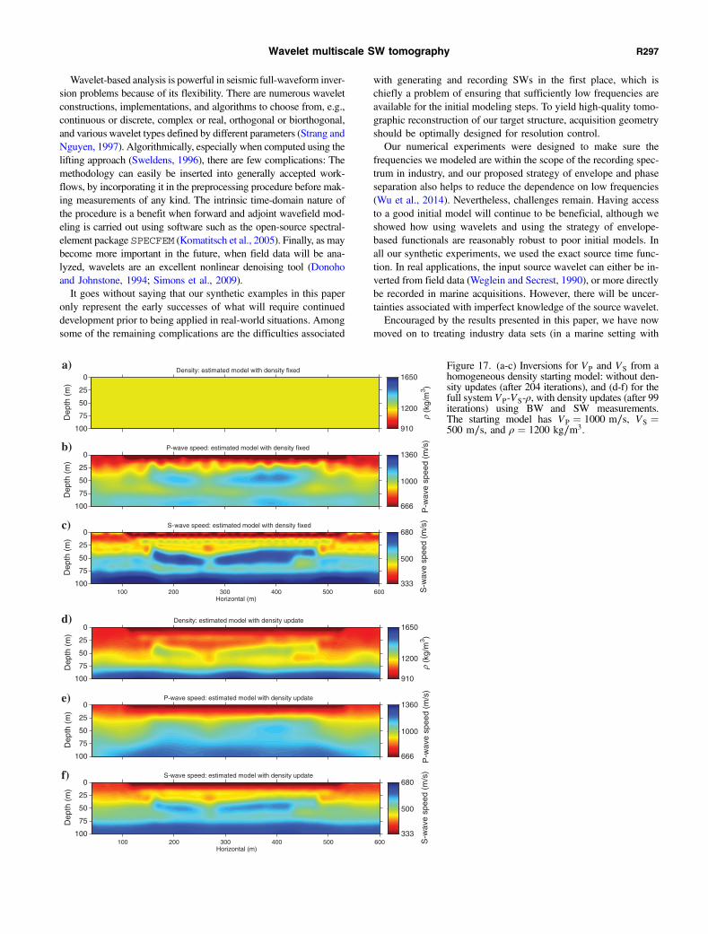
Wavelet-based analysis is powerful in seismic full-waveform inver-sion problems because of its flexibility. There are numerous waveletconstructions, implementations, and algorithms to choose from, e.g.,continuous or discrete, complex or real, orthogonal or biorthogonal,and various wavelet types defined by different parameters (Strang andNguyen, 1997). Algorithmically, especially when computed using thelifting approach (Sweldens, 1996), there are few complications: Themethodology can easily be inserted into generally accepted work-flows, by incorporating it in the preprocessing procedure before mak-ing measurements of any kind. The intrinsic time-domain nature ofthe procedure is a benefit when forward and adjoint wavefield mod-eling is carried out using software such as the open-source spectral-element package SPECFEM (Komatitsch et al., 2005). Finally, as maybecome more important in the future, when field data will be ana-lyzed, wavelets are an excellent nonlinear denoising tool (Donohoand Johnstone, 1994; Simons et al., 2009).It goes without saying that our synthetic examples in this paper

only represent the early successes of what will require continueddevelopment prior to being applied in real-world situations. Amongsome of the remaining complications are the difficulties associated

with generating and recording SWs in the first place, which ischiefly a problem of ensuring that sufficiently low frequencies areavailable for the initial modeling steps. To yield high-quality tomo-graphic reconstruction of our target structure, acquisition geometryshould be optimally designed for resolution control.Our numerical experiments were designed to make sure the

frequencies we modeled are within the scope of the recording spec-trum in industry, and our proposed strategy of envelope and phaseseparation also helps to reduce the dependence on low frequencies(Wu et al., 2014). Nevertheless, challenges remain. Having accessto a good initial model will continue to be beneficial, although weshowed how using wavelets and using the strategy of envelope-based functionals are reasonably robust to poor initial models. Inall our synthetic experiments, we used the exact source time func-tion. In real applications, the input source wavelet can either be in-verted from field data (Weglein and Secrest, 1990), or more directlybe recorded in marine acquisitions. However, there will be uncer-tainties associated with imperfect knowledge of the source wavelet.Encouraged by the results presented in this paper, we have now

moved on to treating industry data sets (in a marine setting with

Dep

th (

m)

Density: estimated model with density fixed0

25

50

75

100ρ

(kg/

m3 )

910

1200

1650

Dep

th (

m)

P-wave speed: estimated model with density fixed0

25

50

75

100 P-w

ave

spee

d (m

/s)

666

1000

1360

Horizontal (m)

Dep

th (

m)

S-wave speed: estimated model with density fixed

100 200 300 400 500 600

0

25

50

75

100

S-w

ave

spee

d (m

/s)

333

500

680

Dep

th (

m)

Density: estimated model with density update0

25

50

75

100

ρ (k

g/m

3 )

910

1200

1650

Dep

th (

m)

P-wave speed: estimated model with density update0

25

50

75

100 P-w

ave

spee

d (m

/s)

666

1000

1360

Horizontal (m)

Dep

th (

m)

S-wave speed: estimated model with density update

100 200 300 400 500 600

0

25

50

75

100

S-w

ave

spee

d (m

/s)

333

500

680

a)

b)

c)

d)

e)

f)

Figure 17. (a-c) Inversions for VP and VS from ahomogeneous density starting model: without den-sity updates (after 204 iterations), and (d-f) for thefull system VP-VS-ρ, with density updates (after 99iterations) using BW and SW measurements.The starting model has VP ¼ 1000 m∕s, VS ¼500 m∕s, and ρ ¼ 1200 kg∕m3.


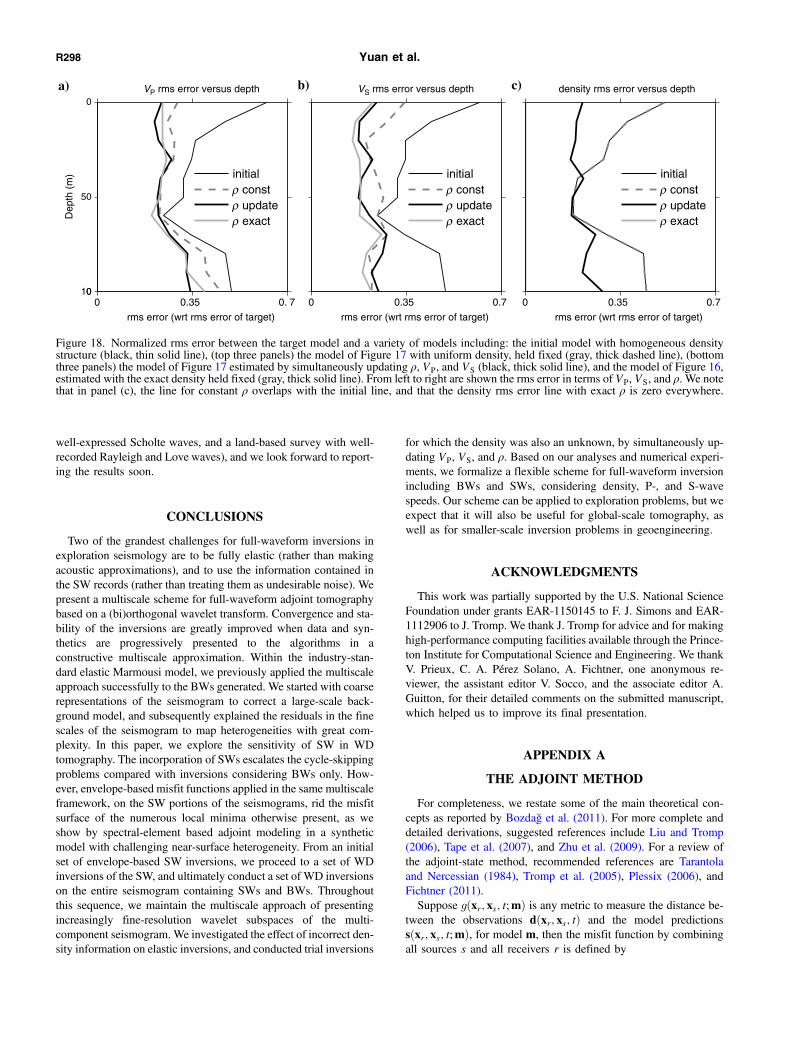
well-expressed Scholte waves, and a land-based survey with well-recorded Rayleigh and Love waves), and we look forward to report-ing the results soon.

CONCLUSIONS

Two of the grandest challenges for full-waveform inversions inexploration seismology are to be fully elastic (rather than makingacoustic approximations), and to use the information contained inthe SW records (rather than treating them as undesirable noise). Wepresent a multiscale scheme for full-waveform adjoint tomographybased on a (bi)orthogonal wavelet transform. Convergence and sta-bility of the inversions are greatly improved when data and syn-thetics are progressively presented to the algorithms in aconstructive multiscale approximation. Within the industry-stan-dard elastic Marmousi model, we previously applied the multiscaleapproach successfully to the BWs generated. We started with coarserepresentations of the seismogram to correct a large-scale back-ground model, and subsequently explained the residuals in the finescales of the seismogram to map heterogeneities with great com-plexity. In this paper, we explore the sensitivity of SW in WDtomography. The incorporation of SWs escalates the cycle-skippingproblems compared with inversions considering BWs only. How-ever, envelope-based misfit functions applied in the same multiscaleframework, on the SW portions of the seismograms, rid the misfitsurface of the numerous local minima otherwise present, as weshow by spectral-element based adjoint modeling in a syntheticmodel with challenging near-surface heterogeneity. From an initialset of envelope-based SW inversions, we proceed to a set of WDinversions of the SW, and ultimately conduct a set of WD inversionson the entire seismogram containing SWs and BWs. Throughoutthis sequence, we maintain the multiscale approach of presentingincreasingly fine-resolution wavelet subspaces of the multi-component seismogram. We investigated the effect of incorrect den-sity information on elastic inversions, and conducted trial inversions

for which the density was also an unknown, by simultaneously up-dating VP, VS, and ρ. Based on our analyses and numerical experi-ments, we formalize a flexible scheme for full-waveform inversionincluding BWs and SWs, considering density, P-, and S-wavespeeds. Our scheme can be applied to exploration problems, but weexpect that it will also be useful for global-scale tomography, aswell as for smaller-scale inversion problems in geoengineering.

ACKNOWLEDGMENTS

This work was partially supported by the U.S. National ScienceFoundation under grants EAR-1150145 to F. J. Simons and EAR-1112906 to J. Tromp. We thank J. Tromp for advice and for makinghigh-performance computing facilities available through the Prince-ton Institute for Computational Science and Engineering. We thankV. Prieux, C. A. Pérez Solano, A. Fichtner, one anonymous re-viewer, the assistant editor V. Socco, and the associate editor A.Guitton, for their detailed comments on the submitted manuscript,which helped us to improve its final presentation.

APPENDIX A

THE ADJOINT METHOD

For completeness, we restate some of the main theoretical con-cepts as reported by Bozdağ et al. (2011). For more complete anddetailed derivations, suggested references include Liu and Tromp(2006), Tape et al. (2007), and Zhu et al. (2009). For a review ofthe adjoint-state method, recommended references are Tarantolaand Nercessian (1984), Tromp et al. (2005), Plessix (2006), andFichtner (2011).Suppose gðxr; xs; t;mÞ is any metric to measure the distance be-

tween the observations dðxr; xs; tÞ and the model predictionssðxr; xs; t;mÞ, for model m, then the misfit function by combiningall sources s and all receivers r is defined by

0 0.35 0. 7

0

50

100

rms error (wrt rms error of target)

Dep

th (

m)

VP rms error versus depth

initialρ constρ updateρ exact

0 0.35 0.7


VS rms error versus depth


0 0.35 0.7


density rms error versus depth


a) b) c)

Figure 18. Normalized rms error between the target model and a variety of models including: the initial model with homogeneous densitystructure (black, thin solid line), (top three panels) the model of Figure 17 with uniform density, held fixed (gray, thick dashed line), (bottomthree panels) the model of Figure 17 estimated by simultaneously updating ρ, VP, and VS (black, thick solid line), and the model of Figure 16,estimated with the exact density held fixed (gray, thick solid line). From left to right are shown the rms error in terms of VP, VS, and ρ. We notethat in panel (c), the line for constant ρ overlaps with the initial line, and that the density rms error line with exact ρ is zero everywhere.

R298 Yuan et al.

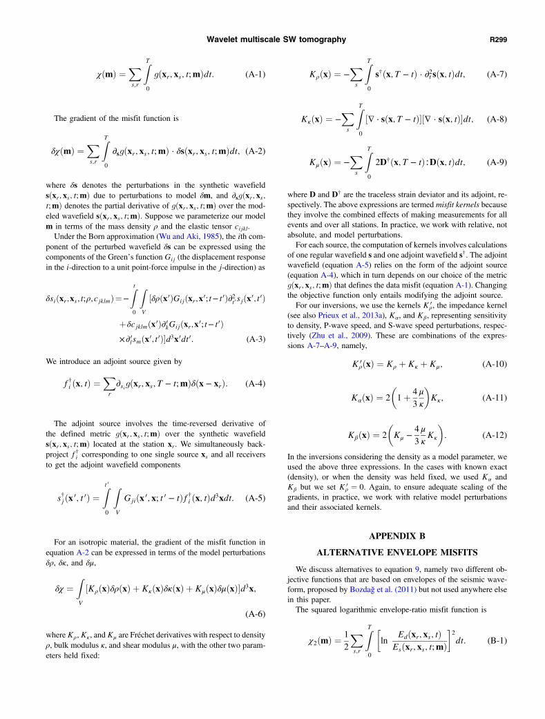
χðmÞ ¼Xs;r

ZT

0

gðxr; xs; t;mÞdt: (A-1)

The gradient of the misfit function is

δχðmÞ ¼Xs;r

ZT

0

∂sgðxr; xs; t;mÞ · δsðxr; xs; t;mÞdt; (A-2)

where δs denotes the perturbations in the synthetic wavefieldsðxr; xs; t;mÞ due to perturbations to model δm, and ∂sgðxr; xs;t;mÞ denotes the partial derivative of gðxr; xs; t;mÞ over the mod-eled wavefield sðxr; xs; t;mÞ. Suppose we parameterize our modelm in terms of the mass density ρ and the elastic tensor cijkl.Under the Born approximation (Wu and Aki, 1985), the ith com-

ponent of the perturbed wavefield δs can be expressed using thecomponents of the Green’s function Gij (the displacement responsein the i-direction to a unit point-force impulse in the j-direction) as

δsiðxr;xs;t;ρ;cjklmÞ¼−Zt

0

ZV

½δρðx 0ÞGijðxr;x 0;t− t 0Þ∂2t0sjðx 0;t 0Þ

þδcjklmðx 0Þ∂ 0kGijðxr;x 0;t− t0Þ×∂ 0lsmðx 0;t 0Þ�d3x 0dt 0: (A-3)

We introduce an adjoint source given by

f†i ðx; tÞ ¼Xr

∂sigðxr; xs; T − t;mÞδðx − xrÞ: (A-4)

The adjoint source involves the time-reversed derivative ofthe defined metric gðxr; xs; t;mÞ over the synthetic wavefieldsðxr; xs; t;mÞ located at the station xr. We simultaneously back-project f†i corresponding to one single source xs and all receiversto get the adjoint wavefield components

s†jðx 0; t 0Þ ¼Zt 0

0

ZV

Gjiðx 0; x; t 0 − tÞf†i ðx; tÞd3xdt: (A-5)

For an isotropic material, the gradient of the misfit function inequation A-2 can be expressed in terms of the model perturbationsδρ, δκ, and δμ,

δχ ¼ZV

½KρðxÞδρðxÞ þ KκðxÞδκðxÞ þ KμðxÞδμðxÞ�d3x;

(A-6)

whereKρ,Kκ , andKμ are Fréchet derivatives with respect to densityρ, bulk modulus κ, and shear modulus μ, with the other two param-eters held fixed:

KρðxÞ ¼ −Xs

ZT

0

s†ðx; T − tÞ · ∂2t sðx; tÞdt; (A-7)

KκðxÞ ¼ −Xs

ZT

0

½∇ ⋅ sðx; T − tÞ�½∇ · sðx; tÞ�dt; (A-8)

KμðxÞ ¼ −Xs

ZT

0

2D†ðx; T − tÞ∶Dðx; tÞdt; (A-9)

where D and D† are the traceless strain deviator and its adjoint, re-spectively. The above expressions are termed misfit kernels becausethey involve the combined effects of making measurements for allevents and over all stations. In practice, we work with relative, notabsolute, and model perturbations.For each source, the computation of kernels involves calculations

of one regular wavefield s and one adjoint wavefield s†. The adjointwavefield (equation A-5) relies on the form of the adjoint source(equation A-4), which in turn depends on our choice of the metricgðxr; xs; t;mÞ that defines the data misfit (equation A-1). Changingthe objective function only entails modifying the adjoint source.For our inversions, we use the kernels K 0

ρ, the impedance kernel(see also Prieux et al., 2013a), Kα, and Kβ, representing sensitivityto density, P-wave speed, and S-wave speed perturbations, respec-tively (Zhu et al., 2009). These are combinations of the expres-sions A-7–A-9, namely,

K 0ρðxÞ ¼ Kρ þ Kκ þ Kμ; (A-10)

KαðxÞ ¼ 2

�1þ 4

3

μ

κ

�Kκ; (A-11)

KβðxÞ ¼ 2

�Kμ −

4

3

μ

κKκ

�: (A-12)

In the inversions considering the density as a model parameter, weused the above three expressions. In the cases with known exact(density), or when the density was held fixed, we used Kα andKβ but we set K 0

ρ ¼ 0. Again, to ensure adequate scaling of thegradients, in practice, we work with relative model perturbationsand their associated kernels.

APPENDIX B

ALTERNATIVE ENVELOPE MISFITS

We discuss alternatives to equation 9, namely two different ob-jective functions that are based on envelopes of the seismic wave-form, proposed by Bozdağ et al. (2011) but not used anywhere elsein this paper.The squared logarithmic envelope-ratio misfit function is

χ2ðmÞ ¼ 1

2

Xs;r

ZT

0

�ln

Edðxr; xs; tÞEsðxr; xs; t;mÞ

�2

dt: (B-1)


Its associated adjoint source takes the same form as equation 16,

f†ðx; tÞ ¼Xr

ðErat2 s −HfErat

2 ½Hfsg�gÞδðx − xrÞ; (B-2)

but with a newly defined ratio Erat2 taking the place of Erat

1 in equa-tion 16, namely,

Erat2 ¼ lnðEsÞ − lnðEdÞ

ðEsÞ2: (B-3)

The weighting of small residuals by the ED misfit function Erat1 is

very different than that by the squared logarithmic envelope ratiomisfit function Erat

2 . In both cases, care has to be taken to avoiddivision by small numbers.A third alternative envelope-based misfit function is to measure

the crosscorrelation envelope-traveltime misfit ΔTE, determined asthe time shift that maximizes the crosscorrelation (Luo and Schus-ter, 1991) of the envelopes of synthetic Es and observed data Ed:

χ3ðmÞ ¼ 1

2

Xs;r

½ΔTEðxr; xs; t;mÞ�2: (B-4)

The corresponding adjoint source has the same expression asequation B-2, but with the ratio Erat

3 replacing Erat2 ,

Erat3 ¼ Mttw

∂tEs

Es; (B-5)

where w is a window function (e.g., from software such as FLEX-WIN; Maggi et al., 2009) applied to the records before taking cross-correlations, and Mtt contains the traveltime shift between theenvelopes of synthetics and observations determined by crosscor-relation, normalized by the temporal integral of the windowed prod-uct of the synthetic envelope and its second time derivative:

Mtt ¼ ΔTERT0 wðtÞ∂ttEsðtÞEsðtÞdt

: (B-6)

The derivations are contained in the work by Luo and Schuster(1991), Marquering et al. (1999), and Dahlen et al. (2000).

REFERENCES

Aki, K., 1957, Space and time spectra of stationary stochastic waves, withspecial reference to microtremors: Bulletin of the Earthquake ResearchInstitute, 35, 415–456.

Bagheri, A., E. Pistone, and P. Rizzo, 2014, Guided ultrasonic wave imagingfor immersed plates based on wavelet transform and probabilistic analy-sis: Research in Nondestructive Evaluation, 25, 63–81, doi: 10.1080/09349847.2013.837212.

Beaty, K. S., D. R. Schmitt, and M. Sacchi, 2002, Simulated annealing in-version of multimode Rayleigh wave dispersion curves for geologicalstructure: Geophysical Journal International, 151, 622–631, doi: 10.1046/j.1365-246X.2002.01809.x.

Beylkin, G., 1992, On the representation of operators in bases of compactlysupported wavelets: SIAM Journal on Numerical Analysis, 29, 1716–1740, doi: 10.1137/0729097.

Bozdağ, E., and J. Trampert, 2008, On crustal corrections in surface wavetomography: Geophysical Journal International, 172, 1066–1082, doi: 10.1111/j.1365-246X.2007.03690.x.

Bozdağ, E., J. Trampert, and J. Tromp, 2011, Misfit functions for full wave-form inversion based on instantaneous phase and envelope measurements:Geophysical Journal International, 185, 845–870, doi: 10.1111/j.1365-246X.2011.04970.x.

Brossier, R., S. Operto, and J. Virieux, 2009, Seismic imaging of complexonshore structures by 2D elastic frequency-domain full-waveform inver-sion: Geophysics, 74, no. 6, WCC105–WCC118, doi: 10.1190/1.3215771.

Buland, R., and C. H. Chapman, 1983, The computation of seismic traveltimes: Bulletin of the Seismological Society of America, 73, 1271–1302.

Bunks, C., F. M. Saleck, S. Zaleski, and G. Chavent, 1995, Multiscale seis-mic waveform inversion: Geophysics, 60, 1457–1473, doi: 10.1190/1.1443880.

Capdeville, Y., and P. Cance, 2015, Residual homogenization for elasticwave propagation in complex media: Geophysical Journal International,200, 984–997, doi: 10.1093/gji/ggu452.

Capon, J., 1969, High-resolution frequency-wavenumber spectrum analysis:Proceedings of the IEEE, 57, 1408–1418, doi: 10.1109/PROC.1969.7278.

Cara, M., J.-J. Lévêque, and V. Maupin, 1984, Density-versus-depth modelsform multimode surface waves: Geophysical Research Letters, 11, 633–636, doi: 10.1029/GL011i007p00633.

Claerbout, J. F., 1992, Earth soundings analysis: Processing versus inver-sion: Blackwell.

Crice, D., 2005, MASW, the wave of the future— Editorial: Journal of Envi-ronmental and Engineering Geophysics, 10, 77–79, doi: 10.2113/JEEG10.2.77.

Dahlen, F. A., and A. Baig, 2002, Fréchet kernels for body-wave amplitudes:Geophysical Journal International, 150, 440–466, doi: 10.1046/j.1365-246X.2002.01718.x.

Dahlen, F. A., S.-H. Hung, and G. Nolet, 2000, Fréchet kernels for finite-frequency traveltimes. Part I: Theory: Geophysical Journal International,141, 157–174, doi: 10.1046/j.1365-246X.2000.00070.x.

Dahlen, F. A., and J. Tromp, 1998, Theoretical global seismology: PrincetonUniversity Press.

Daubechies, I., 1988, Orthonormal bases of compactly supported wavelets:Communications on Pure and Applied Mathematics, 41, 909–996, doi: 10.1002/cpa.3160410705.

Daubechies, I., 1992, Ten lectures on wavelets, CBMS-NSF RegionalConference Series in Applied Mathematics: SIAM.

de Hoop, M. V., L. Qiu, and O. Scherzer, 2012, Local analysis of inverseproblems: Holder stability and iterative reconstruction: Inverse Problems,28, 045001, doi: 10.1088/0266-5611/28/4/045001.

Dobrin, M. B., and C. H. Savit, 1988, Introduction to geophysical prospec-ting, 4th ed.: McGraw-Hill.

Donoho, D. L., and I. M. Johnstone, 1994, Ideal spatial adaptation by wave-let shrinkage: Biometrika, 81, 425–455, doi: 10.1093/biomet/81.3.425.

Droujinine, A., R.-E. Plessix, and F. Ernst, 2012, Integration of dispersioncurve and full waveform inversion techniques for onshore velocity modelbuilding — Inner Mongolia study: 74th Annual International Conferenceand Exhibition, EAGE, Extended Abstracts, doi: 10.3997/2214-4609.20149893.

Dziewoński, A. M., and D. L. Anderson, 1981, Preliminary reference earthmodel: Physics of the Earth and Planetary Interiors, 25, 297–356, doi: 10.1016/0031-9201(81)90046-7.

Ecoublet, P. E., S. C. Singh, C. H. Chapman, and G. M. Jackson, 2002, Bent-ray traveltime tomography and migration without ray tracing: Geophysi-cal Journal International, 149, 633–645, doi: 10.1046/j.1365-246X.2002.01665.x.

Ekström, G., J. Tromp, and E. W. F. Larson, 1997, Measurements and globalmodels of surface wave propagation: Journal of Geophysical Research,102, 8137–8157, doi: 10.1029/96JB03729.

Ewing, W. M., W. S. Jardetzky, and F. Press, 1957, Elastic waves in layeredmedia, International Series in the Earth Sciences: McGraw-Hill.

Favier, N., S. Chevrot, and D. Komatitsch, 2004, Near-field influence onshear wave splitting and traveltime sensitivity kernels: Geophysical JournalInternational, 156, 467–482, doi: 10.1111/j.1365-246X.2004.02178.x.

Fichtner, A., 2011, Full seismic waveform modelling and inversion:Springer.

Fichtner, A., B. L. N. Kennett, H. Igel, and H.-P. Bunge, 2008, Theoreticalbackground for continental-and global-scale full-waveform inversion inthe time-frequency domain: Geophysical Journal International, 175,665–685, doi: 10.1111/j.1365-246X.2008.03923.x.

Fichtner, A., J. Trampert, P. Cupillard, E. Saygin, T. Taymaz, Y. Capdeville,and A. V. nor, 2013, Multiscale full waveform inversion: GeophysicalJournal International, 194, 534–556, doi: 10.1093/gji/ggt118.

Foti, S., 2000, Multistation methods for geotechnical characterization usingsurface waves: Ph.D. thesis, Politecnico di Torino.

Gabriels, P., R. Snieder, and G. Nolet, 1987, In situ measurements of shear-wave velocity in sediments with higher-mode Rayleigh waves: Geophysi-cal Prospecting, 35, 187–196, doi: 10.1111/j.1365-2478.1987.tb00812.x.

Gee, L. S., and T. H. Jordan, 1992, Generalized seismological data function-als: Geophysical Journal International, 111, 363–390, doi: 10.1111/j.1365-246X.1992.tb00584.x.

Gouédard, P., H. Yao, F. Ernst, and R. D. van der Hilst, 2012, Surface waveeikonal tomography in heterogeneous media using exploration data: Geo-physical Journal International, 191, 781–788, doi: 10.1111/j.1365-246X.2012.05652.x.

R300 Yuan et al.

http://dx.doi.org/10.1080/09349847.2013.837212

http://dx.doi.org/10.1080/09349847.2013.837212

http://dx.doi.org/10.1080/09349847.2013.837212

http://dx.doi.org/10.1080/09349847.2013.837212

http://dx.doi.org/10.1080/09349847.2013.837212

http://dx.doi.org/10.1046/j.1365-246X.2002.01809.x






http://dx.doi.org/10.1137/0729097

http://dx.doi.org/10.1137/0729097














http://dx.doi.org/10.1190/1.3215771

http://dx.doi.org/10.1190/1.3215771

http://dx.doi.org/10.1190/1.3215771

http://dx.doi.org/10.1190/1.1443880

http://dx.doi.org/10.1190/1.1443880

http://dx.doi.org/10.1190/1.1443880

http://dx.doi.org/10.1093/gji/ggu452


http://dx.doi.org/10.1109/PROC.1969.7278




http://dx.doi.org/10.1029/GL011i007p00633


http://dx.doi.org/10.2113/JEEG10.2.77

















http://dx.doi.org/10.1002/cpa.3160410705



http://dx.doi.org/10.1088/0266-5611/28/4/045001

http://dx.doi.org/10.1088/0266-5611/28/4/045001

http://dx.doi.org/10.1093/biomet/81.3.425




http://dx.doi.org/10.3997/2214-4609.20149893

http://dx.doi.org/10.3997/2214-4609.20149893

http://dx.doi.org/10.3997/2214-4609.20149893

http://dx.doi.org/10.1016/0031-9201(81)90046-7

http://dx.doi.org/10.1016/0031-9201(81)90046-7







http://dx.doi.org/10.1029/96JB03729

http://dx.doi.org/10.1029/96JB03729













http://dx.doi.org/10.1093/gji/ggt118


http://dx.doi.org/10.1111/j.1365-2478.1987.tb00812.x






http://dx.doi.org/10.1111/j.1365-246X.1992.tb00584.x












Haskell, N. A., 1953, The dispersion of surface waves on multilayered me-dia: Bulletin of the Seismological Society of America, 43, 18–34.

Ivanov, J., R. D. Miller, J. Xia, D. Steeples, and C. B. Park, 2006, Jointanalysis of refractions with surface waves: An inverse solution to the re-fraction-traveltime problem: Geophysics, 71, no. 6, R131–R138, doi: 10.1190/1.2360226.

Jensen, A., and A. la Cour-Harbo, 2001, Ripples in mathematics: Springer.Komatitsch, D., S. Tsuboi, and J. Tromp, 2005, The spectral-elementmethod in seismology, in A. Levander, and G. Nolet, eds., Seismic earth:Array analysis of broadband seismograms: American Geophysical Union,Geophysical Monograph 157, 205–227, doi: 10.1029/157GM13.

Komatitsch, D., and J. P. Vilotte, 1998, The spectral element method: Anefficient tool to simulate the seismic response of 2D and 3D geologicalstructures: Bulletin of the Seismological Society of America, 88, 368–392.

Lai, C. G., and G. J. Rix, 1998, Simultaneous inversion of Rayleigh phasevelocity and attenuation for near-surface site characterization: School ofCivil and Environmental Engineering, Georgia Institute of Technology,Technical report, http://geosystems.ce.gatech.edu/soil_dynamics/docs/Lai_Rix_98.pdf.

Lai, C. G., and G. J. Rix, 1999, Inversion of multi-mode effective dispersioncurves, in M. Jamiolkowski, R. Lancellotta, and D. Lo Presti, eds., Pro-ceedings of the Second International Symposium on pre-failure deforma-tion characteristics of geomaterials: Balkema, 411–418.

Lebedev, S., T. Meier, G. Nolet, and R. D. van der Hilst, 2005, Automatedmulti-mode inversion of surface and S waveforms: Geophysical JournalInternational, 162, 961–964, doi: 10.1111/j.1365-246X.2005.02708.x.

Lévêque, J.-J., and M. Cara, 1985, Inversion of multimode surface wavedata: Evidence for sub-lithospheric anisotropy: Geophysical Journal ofthe Royal Astronomical Society, 83, 753–773, doi: 10.1111/j.1365-246X.1985.tb04336.x.

Liu, Q., and J. Tromp, 2006, Finite-frequency sensitivity kernels based uponadjoint methods: Bulletin of the Seismological Society of America, 96,2383–2397, doi: 10.1785/0120060041.

Luo, Y., R. Modrak, and J. Tromp, 2014, Strategies in adjoint tomography, inW. Freeden, M. Zuhair Nashed, and T. Sonar, eds., Handbook of Geoma-thematics, 2nd ed.: Springer.

Luo, Y., and G. T. Schuster, 1991, Wave-equation traveltime inversion: Geo-physics, 56, 645–653, doi: 10.1190/1.1443081.

Maggi, A., C. Tape, M. Chen, D. Chao, and J. Tromp, 2009, An automatedtime-window selection algorithm for seismic tomography: GeophysicalJournal International, 178, 257–281, doi: 10.1111/j.1365-246X.2009.04099.x.

Mallat, S., 2008, A wavelet tour of signal processing: The sparse way, 3rded.: Academic Press.

Mallat, S. G., 1989, Multifrequency channel decompositions of images andwavelet models: IEEE Transactions on Acoustics, Speech, and SignalProcessing, 37, 2091–2110, doi: 10.1109/29.45554.

Maraschini, M., F. Ernst, S. Foti, and L. V. Socco, 2010, A new misfit func-tion for multimodal inversion of surface waves: Geophysics, 75, no. 4,G31–G43, doi: 10.1190/1.3436539.

Marquering, H., F. A. Dahlen, and G. Nolet, 1999, Three-dimensional sen-sitivity kernels for finite-frequency travel times: The banana-doughnutparadox: Geophysical Journal International, 137, 805–815, doi: 10.1046/j.1365-246x.1999.00837.x.

Masoni, I., R. Brossier, J. Virieux, and J. L. Boelle, 2014, Robust full wave-form inversion of surface waves: 84th Annual International Meeting,SEG, Expanded Abstracts, 1126–1130.

McMechan, G. A., and M. J. Yedlin, 1981, Analysis of dispersive waves bywave field transformation: Geophysics, 46, 869–874, doi: 10.1190/1.1441225.

Miller, G. F., and H. Pursey, 1955, On the partition of energy between elasticwaves in a semi-infinite solid: Proceedings of the Royal Society of Lon-don, Series A, 233, 55–69, doi: 10.1098/rspa.1955.0245.

Miller, R. D., J. Xia, C. B. Park, and J. M. Ivanov, 1999, Multichannel analy-sis of surface waves to map bedrock: The Leading Edge, 18, 1392–1396,doi: 10.1190/1.1438226.

Montagner, J.-P., and N. Jobert, 1988, Vectorial tomography. II: Applicationto the Indian Ocean: Geophysical Journal International, 94, 309–344, doi:10.1111/j.1365-246X.1988.tb05904.x.

Montagner, J.-P., and H.-C. Nataf, 1988, Vectorial tomography. Part I:Theory: Geophysical Journal International, 94, 295–307, doi: 10.1111/j.1365-246X.1988.tb05903.x.

Morlet, J., G. Arens, E. Fourgeau, and D. Giard, 1982a, Wave propagationand sampling theory. Part I: Complex signal and scattering in multilayeredmedia: Geophysics, 47, 203–221, doi: 10.1190/1.1441328.

Morlet, J., G. Arens, E. Fourgeau, and D. Giard, 1982b, Wave propagationand sampling theory. Part II: Sampling theory and complex waves: Geo-physics, 47, 222–236, doi: 10.1190/1.1441329.

Nataf, H.-C., I. Nakanishi, and D. L. Anderson, 1986, Measurements ofmantle wave velocities and inversion for lateral heterogeneities andanisotropy. Part 3: Inversion: Journal of Geophysical Research, 91,7261–7307, doi: 10.1029/JB091iB07p07261.

Nocedal, J., and S. J. Wright, 2006, Numerical optimization: Springer.Nolet, G., 1990, Partitioned waveform inversion and two-dimensional struc-ture under the network of autonomously recording seismographs: Journal ofGeophysical Research, 95, 8499–8512, doi: 10.1029/JB095iB06p08499.

Nolet, G., 2008, A breviary for seismic tomography: Cambridge UniversityPress.

Nolet, G., J. van Trier, and R. Huisman, 1986, A formalism for nonlinearinversion of seismic surface waves: Geophysical Research Letters, 13,26–29, doi: 10.1029/GL013i001p00026.

O’Neill, A., and T. Matsuoka, 2005, Dominant higher surface-wave modesand possible inversion pitfalls: Journal of Environmental and EngineeringGeophysics, 10, 185–201, doi: 10.2113/JEEG10.2.185.

Operto, S., Y. Gholami, R. Brossier, L. Métivier, V. Prieux, A. Ribodetti, andJ. Virieux, 2013, A guided tour of multiparameter full-waveform inver-sion with multicomponent data: From theory to practice: The LeadingEdge, 32, 1040–1054, doi: 10.1190/tle32091040.1.

Park, C. B., R. D. Miller, and J. Xia, 1999, Multichannel analysis of surfacewaves: Geophysics, 64, 800–808, doi: 10.1190/1.1444590.

Pérez Solano, C. A., D. Donno, and H. Chauris, 2014, Alternative waveforminversion for surface wave analysis in 2-D media: Geophysical JournalInternational, 198, 1359–1372, doi: 10.1093/gji/ggu211.

Plessix, R.-E., 2006, A review of the adjoint-state method for computing thegradient of a functional with geophysical applications: Geophysical JournalInternational, 167, 495–503, doi: 10.1111/j.1365-246X.2006.02978.x.

Pratt, R. G., 1999, Seismic waveform inversion in the frequency domain.Part 1: Theory and verification in a physical scale model: Geophysics,64, 888–901, doi: 10.1190/1.1444597.

Pratt, R. G., and R. M. Shipp, 1999, Seismic waveform inversion in the fre-quency domain. Part 2: Fault delineation in sediments using crossholedata: Geophysics, 64, 902–914, doi: 10.1190/1.1444598.

Pratt, R. G., Z.-M. Song, P. Williamson, and M. Warner, 1996, Two-dimen-sional velocity models from wide-angle seismic data by wavefield inver-sion: Geophysical Journal International, 124, 323–340, doi: 10.1111/j.1365-246X.1996.tb07023.x.

Prieux, V., R. Brossier, S. Operto, and J. Virieux, 2013a, Multiparameter fullwaveform inversion of multicomponent ocean-bottom-cable data from theValhall field. Part 1: Imaging compressional wave speed, density and at-tenuation: Geophysical Journal International, 194, 1640–1664, doi: 10.1093/gji/ggt177.

Prieux, V., R. Brossier, S. Operto, and J. Virieux, 2013b, Multiparameter fullwaveform inversion of multicomponent ocean-bottom-cable data from theValhall field. Part 2: Imaging compressive-wave and shear-wave veloc-ities: Geophysical Journal International, 194, 1665–1681, doi: 10.1093/gji/ggt178.

Rawlinson, N., and M. Sambridge, 2003, Seismic traveltime tomography ofthe crust and lithosphere: Advances in Geophysics, 46, 81–198, doi: 10.1016/S0065-2687(03)46002-0.

Rayleigh, J. W. S., 1885, On waves propagated along the plane surface of anelastic solid: Proceedings of the London Mathematical Society, 17, 4–11,doi: 10.1112/plms/s1-17.1.4.

Richart, F. E., J. R. Hall, and R. D. Woods, 1970, Vibrations of soils andfoundations: Prentice-Hall.

Rickers, F., A. Fichtner, and J. Trampert, 2012, Imaging mantle plumes withinstantaneous phase measurements of diffracted waves: Geophysical Jour-nal International, 190, 650–664, doi: 10.1111/j.1365-246X.2012.05515.x.

Ritsema, J., A. A. Deuss, H. J. van Heijst, and J. H. Woodhouse, 2011,S40RTS: A degree-40 shear-velocity model for the mantle from new Ray-leigh wave dispersion, teleseismic traveltime and normal-mode splittingfunction measurements: Geophysical Journal International, 184, 1223–1236, doi: 10.1111/j.1365-246X.2010.04884.x.

Rix, G. J., C. G. Lai, and A. W. S. Jr, 2000, In situ measurement of dampingratio using surface waves: Journal of Geotechnical and GeoenvironmentalEngineering, 126, 472–480, doi: 10.1061/(ASCE)1090-0241(2000)126:5(472).

Rix, G. J., C. G. Lai, M. C. Orozco, G. L. Hebeler, and V. Roma, 2001,Recent advances in surface wave methods for geotechnical site characteri-zation: Presented at XV International Conference on Soil Mechanics andGeotechnical Engineering, 499–502.

Romanowicz, B., 2003, Global mantle tomography: Progress status in the last10 years: Annual Reviews of Geophysics and Space Physics, 31, 303–328.

Romanowicz, B., and D. Giardini, 2001, The future of permanent seismicnetworks: Science, 293, 2000–2001, doi: 10.1126/science.1061771.

Shin, C., and Y. H. Cha, 2008, Waveform inversion in the Laplace domain:Geophysical Journal International, 173, 922–931, doi: 10.1111/j.1365-246X.2008.03768.x.

Sigloch, K., and G. Nolet, 2006, Measuring finite-frequency body-waveamplitudes and traveltimes: Geophysical Journal International, 167,271–287, doi: 10.1111/j.1365-246X.2006.03116.x.

Simons, F. J., B. D. E. Dando, and R. M. Allen, 2006a, Automatic detectionand rapid determination of earthquake magnitude by wavelet multiscaleanalysis of the primary arrival: Earth and Planetary Science Letters, 250,214–223, doi: 10.1016/j.epsl.2006.07.039.


http://dx.doi.org/10.1190/1.2360226

http://dx.doi.org/10.1190/1.2360226

http://dx.doi.org/10.1190/1.2360226

http://dx.doi.org/10.1029/157GM13

http://dx.doi.org/10.1029/157GM13

http://geosystems.ce.gatech.edu/soil_dynamics/docs/Lai_Rix_98.pdf



















http://dx.doi.org/10.1785/0120060041

http://dx.doi.org/10.1785/0120060041

http://dx.doi.org/10.1190/1.1443081

http://dx.doi.org/10.1190/1.1443081

http://dx.doi.org/10.1190/1.1443081







http://dx.doi.org/10.1109/29.45554

http://dx.doi.org/10.1109/29.45554

http://dx.doi.org/10.1109/29.45554

http://dx.doi.org/10.1190/1.3436539

http://dx.doi.org/10.1190/1.3436539

http://dx.doi.org/10.1190/1.3436539

http://dx.doi.org/10.1046/j.1365-246x.1999.00837.x






http://dx.doi.org/10.1190/1.1441225

http://dx.doi.org/10.1190/1.1441225

http://dx.doi.org/10.1190/1.1441225

http://dx.doi.org/10.1098/rspa.1955.0245




http://dx.doi.org/10.1190/1.1438226

http://dx.doi.org/10.1190/1.1438226

http://dx.doi.org/10.1190/1.1438226














http://dx.doi.org/10.1190/1.1441328

http://dx.doi.org/10.1190/1.1441328

http://dx.doi.org/10.1190/1.1441328

http://dx.doi.org/10.1190/1.1441329

http://dx.doi.org/10.1190/1.1441329

http://dx.doi.org/10.1190/1.1441329

http://dx.doi.org/10.1029/JB091iB07p07261










http://dx.doi.org/10.1190/tle32091040.1



http://dx.doi.org/10.1190/1.1444590

http://dx.doi.org/10.1190/1.1444590

http://dx.doi.org/10.1190/1.1444590









http://dx.doi.org/10.1190/1.1444597

http://dx.doi.org/10.1190/1.1444597

http://dx.doi.org/10.1190/1.1444597

http://dx.doi.org/10.1190/1.1444598

http://dx.doi.org/10.1190/1.1444598

http://dx.doi.org/10.1190/1.1444598











http://dx.doi.org/10.1016/S0065-2687(03)46002-0

http://dx.doi.org/10.1016/S0065-2687(03)46002-0

http://dx.doi.org/10.1112/plms/s1-17.1.4
















http://dx.doi.org/10.1061/(ASCE)1090-0241(2000)126:5(472)



http://dx.doi.org/10.1126/science.1061771
















http://dx.doi.org/10.1016/j.epsl.2006.07.039






Simons, F. J., G. Nolet, J. M. Babcock, R. E. Davis, and J. A. Orcutt, 2006b,A future for drifting seismic networks: Eos — Transactions of the Ameri-can Geophysical Union, 87, 305–307, doi: 10.1029/2006EO310002.

Simons, F. J., G. Nolet, P. Georgief, J. M. Babcock, L. A. Regier, and R. E.Davis, 2009, On the potential of recording earthquakes for global seismictomography by low-cost autonomous instruments in the oceans: Journalof Geophysical Research, 114, B05307, doi: 10.1029/2008JB006088.

Simons, F. J., and R. D. van der Hilst, 2003, Seismic and mechanicalanisotropy and the past and present deformation of the Australian litho-sphere: Earth and Planetary Science Letters, 211, 271–286, doi: 10.1016/S0012-821X(03)00198-5.

Sirgue, L., and R. G. Pratt, 2004, Efficient waveform inversion and imaging:A strategy for selecting temporal frequencies: Geophysics, 69, 231–248,doi: 10.1190/1.1649391.

Snieder, R., 1988a, Large-scale waveform inversions of surface waves for lat-eral heterogeneity. Part 1: Theory and numerical examples: Journal of Geo-physical Research, 93, 12055–12065, doi: 10.1029/JB093iB10p12055.

Snieder, R., 1988b, Large-scale waveform inversions of surface waves forlateral heterogeneity. Part 2: Application to surface waves in Europe andthe Mediterranean: Journal of Geophysical Research, 93, 12067–12080,doi: 10.1029/JB093iB10p12067.

Socco, L. V., S. Foti, and D. Boiero, 2010, Surface-wave analysis for buildingnear-surface velocity models — Established approaches and new perspec-tives: Geophysics, 75, no. 5, 75A83–75A102, doi: 10.1190/1.3479491.

Socco, L. V., and C. Strobbia, 2004, Surface-wave method for near-surfacecharacterization: A tutorial: Near Surface Geophysics, 2, 165–185.

Stokoe, K. H., J. Sung-Ho, and R. D. Woods, 2004, Some contributions of insitu geophysical measurements to solving geotechnical engineering prob-lems: Geotechnical and geophysical site characterization: Proceedings ofthe 2nd International Conference on Site Characterization, InternationalSociety of Soil Mechanics and Geotechnical Engineering, 97–132.

Strang, G., and T. Nguyen, 1997, Wavelets and filter banks, 2nd ed.: Well-esley-Cambridge Press.

Stutzmann, E., and J.-P. Montagner, 1993, An inverse technique for retriev-ing higher mode phase velocity and mantle structure: Geophysical JournalInternational, 113, 669–683, doi: 10.1111/j.1365-246X.1993.tb04659.x.

Stutzmann, E., and J.-P. Montagner, 1994, Tomography of the transition zonefrom the inversion of higher-mode surface-waves: Physics of the Earth andPlanetary Interiors, 86, 99–115, doi: 10.1016/0031-9201(94)05064-3.

Sweldens, W., 1996, The lifting scheme: A custom-design construction ofbiorthogonal wavelets: Applied and Computational Harmonic Analysis,3, 186–200, doi: 10.1006/acha.1996.0015.

Tape, C., Q. Liu, and J. Tromp, 2007, Finite-frequency tomography usingadjoint methods — Methodology and examples using membrane surfacewaves: Geophysical Journal International, 168, 1105–1129, doi: 10.1111/j.1365-246X.2006.03191.x.

Tarantola, A., 1984a, Inversion of seismic reflection data in the acousticapproximation: Geophysics, 49, 1259–1266, doi: 10.1190/1.1441754.

Tarantola, A., 1984b, Linearized inversion of seismic reflection data: Geophysi-cal Prospecting, 32, 998–1015, doi: 10.1111/j.1365-2478.1984.tb00751.x.

Tarantola, A., and A. Nercessian, 1984, Three-dimensional inversion with-out blocks: Geophysical Journal of the Royal Astronomical Society, 76,299–306, doi: 10.1111/j.1365-246X.1984.tb05047.x.

Thompson, D. O., and D. E. Chimenti, 1997, Review of progress in quan-titative nondestructive evaluation 16th ed.: Springer.

Tian, Y., R. Montelli, G. Nolet, and F. A. Dahlen, 2007, Computing trav-eltime and amplitude sensitivity kernels in finite-frequency tomography:Journal of Computational Physics, 226, 2271–2288, doi: 10.1016/j.jcp.2007.07.004.

Tokimatsu, K., S. Tamura, and H. Kojima, 1992, Effects of multiple modeson Rayleigh wave dispersion characteristics: Journal of Geotechnical En-gineering, 118, 1529–1543, doi: 10.1061/(ASCE)0733-9410(1992)118:10(1529).

Trampert, J., and J. H. Woodhouse, 2003, Global anisotropic phase velocitymaps for fundamental mode surface waves between 40 and 150 s: Geo-physical Journal International, 154, 154–165, doi: 10.1046/j.1365-246X.2003.01952.x.

Tromp, J., C. Tape, and Q. Liu, 2005, Seismic tomography, adjoint methods,time reversal and banana-doughnut kernels: Geophysical JournalInternational, 160, 195–216, doi: 10.1111/j.1365-246X.2004.02453.x.

VanDecar, J. C., and R. S. Crosson, 1990, Determination of teleseismicrelative phase arrival times using multi-channel cross-correlation andleast squares: Bulletin of the Seismological Society of America, 80,150–169.

van Heijst, H. J., and J. H. Woodhouse, 1997, Measuring surface-wave over-tone phase velocities using a mode-branch stripping technique: Geophysi-cal Journal International, 131, 209–230, doi: 10.1111/j.1365-246X.1997.tb01217.x.

Van Heijst, H. J., and J. H. Woodhouse, 1999, Global high-resolution phasevelocity distributions of overtone and fundamental-mode surface wavesdetermined by mode branch stripping: Geophysical Journal International,137, 601–620, doi: 10.1046/j.1365-246x.1999.00825.x.

Weglein, A. B., and B. G. Secrest, 1990, Wavelet estimation for a multidi-mensional acoustic or elastic earth: Geophysics, 55, 902–913, doi: 10.1190/1.1442905.

Woodhouse, J. H., 1974, Surface waves in a laterally varying layered struc-ture: Geophysical Journal of the Royal Astronomical Society, 37, 461–490, doi: 10.1111/j.1365-246X.1974.tb04098.x.

Woodhouse, J. H., and A. M. Dziewoński, 1984, Mapping the upper mantle:Three-dimensional modeling of earth structure by inversion of seismicwaveforms: Journal of Geophysical Research, 89, 5953–5986, doi: 10.1029/JB089iB07p05953.

Wu, R.-S., and K. Aki, 1985, Scattering characteristics of elastic waves by anelastic heterogeneity: Geophysics, 50, 582–595, doi: 10.1190/1.1441934.

Wu, R.-S., J. Luo, and B. Wu, 2014, Seismic envelope inversion and modu-lation signal model: Geophysics, 79, no. 3, WA13–WA24, doi: 10.1190/geo2013-0294.1.

Xia, J., R. D. Miller, and C. B. Park, 1999, Estimation of near-surface shear-wave velocity by inversion of Rayleigh waves: Geophysics, 64, 691–700,doi: 10.1190/1.1444578.

Xia, J., R. D. Miller, C. B. Park, and G. Tian, 2002, Determining Q of near-surface materials from Rayleigh waves: Journal of Applied Geophysics,51, 121–129, doi: 10.1016/S0926-9851(02)00228-8.

Yuan, D., and S. Nazarian, 1993, Automated surface wave method: Inversiontechnique: Journal of Geotechnical Engineering, 119, 1112–1126, doi: 10.1061/(ASCE)0733-9410(1993)119:7(1112).

Yuan, Y. O., and F. J. Simons, 2014, Multiscale adjoint waveform-differencetomography using wavelets: Geophysics, 79, no. 3, WA79–WA95, doi: 10.1190/geo2013-0383.1.

Yuan, Y. O., F. J. Simons, and E. Bozdağ, 2014, Full-waveform adjointtomography in a multiscale perspective: 84th Annual International Meet-ing, SEG, Expanded Abstracts, 1194–1199.

Zhang, S. X., and L. S. Chan, 2003, Possible effects of misidentified modenumber on Rayleigh wave inversion: Journal of Applied Geophysics, 53,17–29, doi: 10.1016/S0926-9851(03)00014-4.

Zhu, H., Y. Luo, T. Nissen-Meyer, C. Morency, and J. Tromp, 2009, Elasticimaging and time-lapse migration based on adjoint methods: Geophysics,74, no. 6, WCA167–WCA177, doi: 10.1190/1.3261747.

R302 Yuan et al.

http://dx.doi.org/10.1029/2006EO310002

http://dx.doi.org/10.1029/2006EO310002

http://dx.doi.org/10.1029/2008JB006088

http://dx.doi.org/10.1029/2008JB006088

http://dx.doi.org/10.1016/S0012-821X(03)00198-5

http://dx.doi.org/10.1016/S0012-821X(03)00198-5

http://dx.doi.org/10.1016/S0012-821X(03)00198-5

http://dx.doi.org/10.1190/1.1649391

http://dx.doi.org/10.1190/1.1649391

http://dx.doi.org/10.1190/1.1649391





http://dx.doi.org/10.1190/1.3479491

http://dx.doi.org/10.1190/1.3479491

http://dx.doi.org/10.1190/1.3479491







http://dx.doi.org/10.1016/0031-9201(94)05064-3

http://dx.doi.org/10.1016/0031-9201(94)05064-3

http://dx.doi.org/10.1006/acha.1996.0015











http://dx.doi.org/10.1190/1.1441754

http://dx.doi.org/10.1190/1.1441754

http://dx.doi.org/10.1190/1.1441754













http://dx.doi.org/10.1016/j.jcp.2007.07.004

































http://dx.doi.org/10.1190/1.1442905

http://dx.doi.org/10.1190/1.1442905

http://dx.doi.org/10.1190/1.1442905









http://dx.doi.org/10.1190/1.1441934

http://dx.doi.org/10.1190/1.1441934

http://dx.doi.org/10.1190/1.1441934

http://dx.doi.org/10.1190/geo2013-0294.1




http://dx.doi.org/10.1190/1.1444578

http://dx.doi.org/10.1190/1.1444578

http://dx.doi.org/10.1190/1.1444578

http://dx.doi.org/10.1016/S0926-9851(02)00228-8

http://dx.doi.org/10.1016/S0926-9851(02)00228-8






http://dx.doi.org/10.1016/S0926-9851(03)00014-4

http://dx.doi.org/10.1016/S0926-9851(03)00014-4

http://dx.doi.org/10.1190/1.3261747

http://dx.doi.org/10.1190/1.3261747

http://dx.doi.org/10.1190/1.3261747

Download - Multiscale adjoint waveform tomography for surface …€¦ · · 2015-09-10Multiscale adjoint waveform tomography for surface ... of fundamental-mode and overtone SWs via a mode-branch

Top Related