
Department of Electronics and Communication Engineering – MSEC
M.S ENGINEERING COLLEGE
NAVARTNA AGRAHARA,SADAHALLI P.O
BANGALORE-562110
Department of Electronics and Communication
Digital signal Processing Lab [10ECL57]
V SEM
Prepared by:
Naveen H

Page | 1 Department of Electronics and Communication Engineering – MSEC
C O N T E N T S
I. QUESTION BANK…………………………………………………………………………..…………….01
II. MATLAB PROGRAMS
1. SAMPLING…………………………………………………………………………………..……03
2. IMPULSE RESPONSE………………………………………………………………..……….06
3. N-PT DFT………………………………………………………………………………………..…09
4. LINEAR CONVOLUTION…………………………………………………………………….13
5. CIRCULAR CONVOLUTION………………………………………………………………..16
6. LINEAR CONVOLUTION USING DFT AND IDFT METHOD………………… .20
7. CIRCULAR CONVOLUTION USING DFT AND IDFT METHOD……………..24
8. AUTO CORRELATION………………………………………………………………………..28
9. CROSS CORRELATION……………………………………………………………………….32
10. DIFFERENCE EQUATION……………………………………………………………………35
11. IIR BUTTERWORTH FILTER……………………………………………………………….38
12. IIR CHEBYSHEV ………………………………………………………………………………..42
13. FIR FILTER…………………………………………………………………………………………46
III. CCS PROGRAMS
1. LINEAR CONVOLUTION ……………………………………………………………………68
2. CIRCULAR CONVOLUTION………………………………………………………………..70
3. IMPULSE RESPONSE…………………………………………………………………………73
4. COMPUTING DFT………………………………………………………………………………75

Page | 2 Department of Electronics and Communication Engineering – MSEC
Q U E S T I O N B A N K
A. MATLAB Programs:
1) Using MATLAB sample, a band limited-continuous time signal with fm=400Hz under
the following conditions :
a. Nyquist rate (correct sampling)
b. Twice the nyquist rate(oversampling)
c. Under sampling
2) Using MATLAB compute the impulse response of a system described by the
difference equation
3) Using MATLAB compute the N-pt DFT of the sequence x(n) given as:
a) x(n)=1,1,1,1; N=4
b) x(n)=1,1,1,1; N=8
4) Using MATLAB compute the linear convolution of the given two sequences
5) Using MATLAB compute the circular convolution of the given two sequences
6) Using MATLAB compute the linear convolution of the given two sequences using DFT
and IDFT method
7) Using MATLAB compute the circular convolution of the given two sequences using
DFT and IDFT method
8) Using MATLAB compute the auto correlation of the given sequences and verify its
properties
9) Using MATLAB compute the cross correlation of the given two sequences
10) Using MATLAB find a solution for the difference equation
11) Realize an IIR filter with:
a. pass-band edge at 1500Hz
b. stop-band edge at 2000Hz
c. sampling frequency of 8000Hz
d. pass-band attenuation is 1dB
e. stop-band attenuation is 15dB
Use Butterworth prototype design & Bilinear Transformation
12) Realize an IIR filter with:
a. pass-band edge at 1500Hz
b. stop-band edge at 2000Hz
c. sampling frequency of 8000Hz
d. pass-band attenuation is 1dB
e. stop-band attenuation is 15dB
Use Chebyshev prototype design & Bilinear Transformation
13) Using MATLAB design an FIR filter to meet the following specifications choosing
Hamming Window:

Page | 3 Department of Electronics and Communication Engineering – MSEC
a. Window Length N=27
b. Cut-off frequency=10Hz
c. Sampling frequency=1000Hz
B. Code Composer Studio Programs:
1) Find out the discrete time convolution of the sequences x(n)=1,2,3,4,5 and
h(n)=1,2,3,4 using code composer studio. Verify the results graphically.
2) Perform the Circular Convolution of the given sequence using Code Composer
Studio.
3) Compute the response of the system whose co-efficient are a0=0.1311, a1=0.2622,
a2=0.1311 and b0=1, b1= -0.7478, b2=0.2722, when the input is a unit impulse signal.
4) Compute the DFT of a sequence using code composer studio.

Page | 4 Department of Electronics and Communication Engineering – MSEC
M A T L A B P R O G R A M S
P R O G R A M 1
TITLE:
Verification of Sampling Theorem
THEORY:
Sampling theorem can be stated in two forms: -
If a finite energy signal g(t) contains no frequencies higher than ‘w’ Hz, it is completely
determined by specifying its ordinates at a sequence of points spaced 1/2w sec apart.
If a finite energy signal g(t) contains no frequencies higher than ‘w’ Hz, it may be completely
recovered from its ordinates at a sequence of points spaced 1/2w sec apart.
The minimum sampling rate of 2w samples per second, for a signal bandwidth of ‘w’Hz is called
NYQUIST RATE.
fs = 2fm
where,
ƒs=Sampling Frequency
ƒm=Message frequency
We encounter these conditions in Sampling Theorem, they are Right sampling, Under sampling and
Over sampling
.
Right Sampling → ƒs = 2ƒm
Under Sampling → ƒs ≤ 2ƒm
Right Sampling → ƒs ≥ 2ƒm
MATLAB CODE:
%Nyquist Rate Sampling
N=input('Enter the Length: ');

Page | 5 Department of Electronics and Communication Engineering – MSEC
subplot(2,2,1);
n=0:1:N-1;
y=ones(size(n))
stem(n,y);
xlabel('Time');
ylabel('Amplitude');
title('Unit Step');
%Under Sampling
n=0:0;
subplot(2,2,2);
y=ones(size(n))
stem(n,y);
xlabel('Time');
ylabel('Amplitude');
title('Unit Impulse');
%Over Sampling
ƒs=1000;
t=0:1/ ƒs:256/ ƒs;
X=sin(2*pi*400*t);
Xm=abs(fft(X));
K=0:length(X)-1;
Subplot(2,2,3);
Stem(k,Xm);
xlabel(‘Hz’);
ylabel(‘Magnitude’);
title(‘Over Sampling’);

Page | 6 Department of Electronics and Communication Engineering – MSEC
OUTPUT:

Page | 7 Department of Electronics and Communication Engineering – MSEC
P R O G R A M 2
TITLE:
Using MATLAB compute the impulse response of a system described by the difference
equation
THEORY:
The response of the system when the input is an impulse function applied at t=0 or n=0 is
defined as the impulse response or unit sample response of the system. The impulse response
completely characterizes the behavior of any LTI system.
If the input to a linear system is expressed as a weighted superposition of time-shifted
impulses, then the output is a weighted superposition of the system responses to each time-shifted
impulse. If the system is also time-invariant, then the system response to a time-shifted impulse is a
time-shifted version of the system response to an impulse. Hence the output of a LTI system is given
by a weighted superposition of time-shifted impulse responses. This weighted superposition is
known as the convolution sum for discrete-time systems and the convolution integral for
continuous-time systems.
Let us consider a LTI system represented by operator T . having input is x(n) and output y(n)
x(n) y(n)
Then impulse response of the system is Tδ(n) = h(n)
CALCULATIONS:
Y(z) - 3/4 Y(z)z-1 + 1/8 Y(z)z-2 = X(z) - 1/3 X(z) z-1
H(z) = Y(z) / X (z) = (1-1/3 z-1) / (1-3/4 z-1+1/8 z-2)
Applying partial fractions,
H(z) = (1-1/3 z-1) / (1-1/2 z-1)(1-1/4 z-1) = A / (1-1/2 z-1) + B / (1-1/4 z-1)
A=2/3;
B=1/3;
H(z) = (2/3) / (1-1/2 z-1) + (1/3) / (1-1/4 z-1)
h(n) = (2/3) (1/2)n u(n) + (1/3) (1/4)n u(n)
LTI System

Page | 8 Department of Electronics and Communication Engineering – MSEC
h(0)=1 h(4)=0.0429 h(8)=0.0026
h(1)=0.416 h(5)=0.02116 h(9)=0.0013
h(2)=0.187 h(6)=0.0105
h(3)=0.088 h(7)=0.0052
MATLAB CODE:
N=input(‘enter the length of imp response’);
b=input('type in numerator coeff=');
a=input('type in denominator coeff=');
[r ,p ,k]=residuez(b,a)
[h,t]=impz(b,a,N)
stem(t,h);
grid;
xlabel('time index');
ylabel('amplitude');
title('impulse response');
INPUT:
Enter the length of imp response 5
Type in numerator coeff=[1 -1/3]
Type in denominator coeff=[1 -3/4 1/8]
OUTPUT:
r =
0.6667
0.3333
p =

Page | 9 Department of Electronics and Communication Engineering – MSEC
0.5000
0.2500
k =
[]
h =
1.0000
0.4167
0.1875
0.0885
0.0430
t =
0
1
2
3
4

Page | 10 Department of Electronics and Communication Engineering – MSEC
P R O G R A M 3
TITLE:
N-point DFT for a given sequence x(n) = 1,1,1,1 for the following:
i. Take N = 4
ii. Take N = 8
THEORY:
Discrete Fourier Transform (DFT) is defined by
; K=0,1,2,............N-1
Here k indicates the index of frequency.
CALCULATIONS:
Take N=8
; K=0,1,2,............N-1
For 8-pt DFT above equation becomes
; K=0,1,..7
This equation is formulated in the matrix form by equation
; n=0,1..N-1
; n=0,1..7
Where

Page | 11 Department of Electronics and Communication Engineering – MSEC
By solving, we get
Magnitude of X[k]=[4,2.613,0,1.082,0,1.082,0,2,613]
Angle of X[k]=[0,-1.178,0,-0.392,0,0.392,0,1.178]
Take N=4
; K=0,1,2,............N-1
For 4-pt DFT above eqn becomes
; K=0,1,..3
This equation is formulated in the matrix form by equation
; n=0,1..N-1
; n=0,1..3
Where
By solving, we get
Magnitude of X[k]=[4,0,0,0]
Angle of X[k]=[0,0,0,0]
MATLAB CODE:
x1=input('enter the sequence x1=');
N=input('enter the value of N=');
xk=fft(x1,N)
subplot(2,2,1);
n=0:1:length(xk)-1;
stem(n,abs(xk));
disp(abs(xk));
xlabel('time index');
ylabel('amplitude');
title('magnitude plot');
subplot(2,2,2);

Page | 12 Department of Electronics and Communication Engineering – MSEC
stem(n,angle(xk));
disp(angle(xk));
xlabel('time index');
ylabel('amplitude');
title('angle plot');
xk1=ifft(xk,N)
subplot(2,2,3);
stem(n,(xk1));
xlabel('time index');
ylabel('amplitude');
title('inverse fourier transform');
INPUT:
i. Enter the sequence x1= [ 1 1 1 1]
Enter the value of N = 4
ii. Enter the sequence x1= [ 1 1 1 1]
Enter the value of N = 8
OUTPUT:
i.

Page | 13 Department of Electronics and Communication Engineering – MSEC
ii.

Page | 14 Department of Electronics and Communication Engineering – MSEC
P R O G R A M 4
TITLE:
Compute linear convolution of the given two sequences
THEORY:
Linear convolution can be performed on unequal sequences length. if a and b are two sequences
then a * b defined as:
The asterisk operator is used to denote convolution.
CALCULATIONS:
1 2 3 4 5
2 2 4 6 8 10
3 3 6 9 12 15
4 4 8 12 16 20
Y = [2,7,16,25,34,31,20]

Page | 15 Department of Electronics and Communication Engineering – MSEC
MATLAB CODE:
X1=input('First Sequence');
X2=input('Second Sequence');
subplot(2,2,1);$
n1=0:1:length(X1)-1;
stem(n1,);
xlabel('Time');
ylabel('Amplitude');
title('First sequence');
subplot(2,2,2);
n2=0:1:length(X2)-1;
stem(n2,X2);
xlabel('Time');
ylabel('Amplitude');
title('Second Sequence');
Y=conv(X1,X2)
subplot(2,2,3);
n3=0:1:length(Y)-1;
stem(n3,Y);
xlabel('Time');
ylabel('Amplitude');
title('Linear Convolution Output');
INPUT:
Enter the first sequence:[1 2 3 4]
Enter the second sequence:[2 3 4]

Page | 16 Department of Electronics and Communication Engineering – MSEC
OUTPUT:

Page | 17 Department of Electronics and Communication Engineering – MSEC
P R O G R A M 5
TITLE:
Perform the Circular convolution for given sequence
a. x(n) = 1,2,3,4
h(n) = 4,3,2,2
b. x(n) = 1,2,3,1
h(n) = 2,1
THEORY:
Circular convolution can be performed only on sequences with equal length.
Let x(n) and h(n) be the two sequences of equal length N.
Then,
Circular convolution can be defined as
y(n) = x(n) ( * ) N h (n)
= ; 0≤n≤N-1
y(n) =
CALCULATIONS:
Given x(n)=1,2,3,4
h(n)=4,3,2,2
y = y + x(m) * h(mod(n-m, N) +1) ; n, m= 1,2,3,4
Initially y=0,0,0,0
for m=1, (1,2,3,4) (4,3,2,2) y=0,0,0,0+4,3,2,2=4,3,2,2
for m=2, (1,2,3,4) (2,4,3,2,) y=4,3,2,2+4,8,6,4=8,11,8,6
for m=3, (1,2,3,4) (,2,2,4,3) y=6,6,12,9+8,11,8,6=14,17,20,15
for m=4, (1,2,3,4) (3,2,2,4,) y=14,17,20,15+12,8,8,16=26,25,28,31
y(n)=26,25,28,31
(OR)

Page | 18 Department of Electronics and Communication Engineering – MSEC
Matrix method:
Y(n)=26,25,28,31
MATLAB CODE:
x=input('Enter the sequence x(n) ');
h=input('Enter the sequence h(h) ');
N1=length(x);
N2=length(h);
N=max(N1,N2);
N3=N1N2;
if(N3>0)
h=[h zeros(1,abs(N3))];
else
x=[x zeros(1,abs(N3));];
end
disp('Sequence x(n) ');
disp(x);
disp('Sequence h(n) ');
disp(h);
n=1:N;
disp(n);
y=0;
for m=1:N
disp(m);
y=y+x(m)*h(mod(n-m,N)+1)
end

Page | 19 Department of Electronics and Communication Engineering – MSEC
disp('circular covolution');
disp(y);
subplot(2,2,1);
stem(n,x);
title('Sequence x(n)');
xlabel('n');
ylabel('Amplitude');
subplot(2,2,2);
stem(n,h);
title('Sequence h(n)');
xlabel('n');
ylabel('Amplitude');
subplot(2,2,3);
stem(n,y);
title('Sequence y(n)');
xlabel('n');
ylabel('Amplitude');
INPUT:
a. Enter the sequence x(n) = [1 2 3 4]
Enter the sequence h(n) = [4 3 2 2]
b. Enter the sequence x(n) = [1 2 3 1]
Enter the sequence h(n) = [2 1]
OUTPUT:
1.

Page | 20 Department of Electronics and Communication Engineering – MSEC
2.

Page | 21 Department of Electronics and Communication Engineering – MSEC
P R O G R A M 6
TITLE:
To perform linear convolution using DFT and IDFT method
THEORY:
Linear convolution can be performed on unequal sequences length. if a and b are two sequences
then a * b defined as:
The asterisk operator is used to denote convolution.
CALCULATIONS:
x1(n) = 2,3,4 ; length of x1(n) [L1] =3
x2(n) = 2,1 ; length of x2(n) [L2] = 2
N = L1 + L2 – 1 = 4;
Therefore x1(n) = 2,3,4,0
x2(n) = 2,1,0,0
Finding the DFT for x1(n) using matrix method:
X1(k) = 9,-2-3j,3,-2+3j
Finding the DFT for x2(n) using matrix method:
X2(k) = 3,2-j,1,2+j
Finding Y(k), Y(k) = X1(k)Y1(k) according to convolution property in DFT:

Page | 22 Department of Electronics and Communication Engineering – MSEC
Y(k) = 27,-7-4j,3,-7+4j
Taking IDFT to find y(n) using matrix method:
y(n) = 4,8,11,4
MATLAB CODE :
x1=input('Enter the sequence x1(n) ');
x2=input('Enter the sequence x2(n) ');
N1=length(x1);
N2=length(x2);
N3=N1+N2-1;
if (N3>N2)
x2=[x2 zeros(1,N3-N2)];
end
if (N3>N1)
x1=[x1 zeros(1,N3-N1)];
end
X1=fft(x1,N3)
X2=fft(x2,N3)
Y=X1.*X2;
y=ifft(Y,N3)
subplot(3,1,1);
n1=0:1:length(x1)-1;

Page | 23 Department of Electronics and Communication Engineering – MSEC
stem(n1,x1);
xlabel('Time');
ylabel('Amplitude');
title('First Sequence');
subplot(3,1,2);
n2=0:1:length(x2)-1;
stem(n2,x2);
xlabel('Time');
ylabel('Amplitude');
title('Second Sequence');
subplot(3,1,3);
n=0:1:length(y)-1;
stem(n,y);
xlabel('Time');
ylabel('Amplitude');
title('Linear Convolution using DFT and IDFT');
INPUT:
Enter the first sequence=[2 3 4]
Enter the second sequence=[2 1]
OUTPUT:

Page | 24 Department of Electronics and Communication Engineering – MSEC

Page | 25 Department of Electronics and Communication Engineering – MSEC
P R O G R A M 7
TITLE:
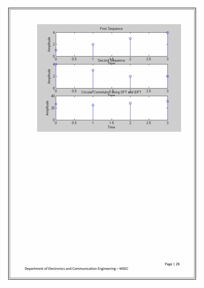
To perform circular convolution using DFT and IDFT
THEORY:
Circular convolution can be performed only on sequences with equal length.
Let x(n) and h(n) be the two sequences of equal length N.
Then,
Circular convolution can be defined as
y(n) = x(n) ( * ) N h (n)
= ; 0≤n≤N-1
y(n) =
CALCULATIONS:
x1(n) = 1,2,3,4
x2(n) = 4,3,2,2
Finding the DFT for x1(n) using matrix method:
X1(k) = 10,-2+2j,-2,-2-2j
Finding the DFT for x2(n) using matrix method:
X2(k) = 11,2-j,1,2+j

Page | 26 Department of Electronics and Communication Engineering – MSEC
Finding Y(k), Y(k) = X1(k)Y1(k) according to convolution property in DFT:
Y(k) = 110,-2+6j,-2,-2-6j
Taking IDFT to find y(n) using matrix method:
y(n) = 26,25,28,31
MATLAB CODE:
x1=input('Enter the sequence x1(n) ');
x2=input('Enter the sequence x2(h) ');
N1=length(x1);
N2=length(x2);
N=max(N1,N2);
N3=N1-N2;
if(N3>0)
x2=[x2 zeros(1,abs(N3))];
else
x1=[x1 zeros(1,abs(N3));];
end
X1=fft(x1,N)
X2=fft(x2,N)
Y=X1.*X2;
y=ifft(Y,N)
subplot(3,1,1);

Page | 27 Department of Electronics and Communication Engineering – MSEC
n1=0:1:length(x1)-1;
stem(n1,x1);
xlabel('Time');
ylabel('Amplitude');
title('First Sequence');
subplot(3,1,2);
n2=0:1:length(x2)-1;
stem(n2,x2);
xlabel('Time');
ylabel('Amplitude');
title('Second Sequence');
subplot(3,1,3);
n=0:1:length(Y)-1;
stem(n,y);
xlabel('Time');
ylabel('Amplitude');
title('Circular Convolution using DFT and IDFT');
INPUT:
Enter the first sequence:[1 2 3 4]
Enter the second sequence:[4 3 2 2]
OUTPUT:
Page | 28 Department of Electronics and Communication Engineering – MSEC

Page | 29 Department of Electronics and Communication Engineering – MSEC
P R O G R A M 8
TITLE:
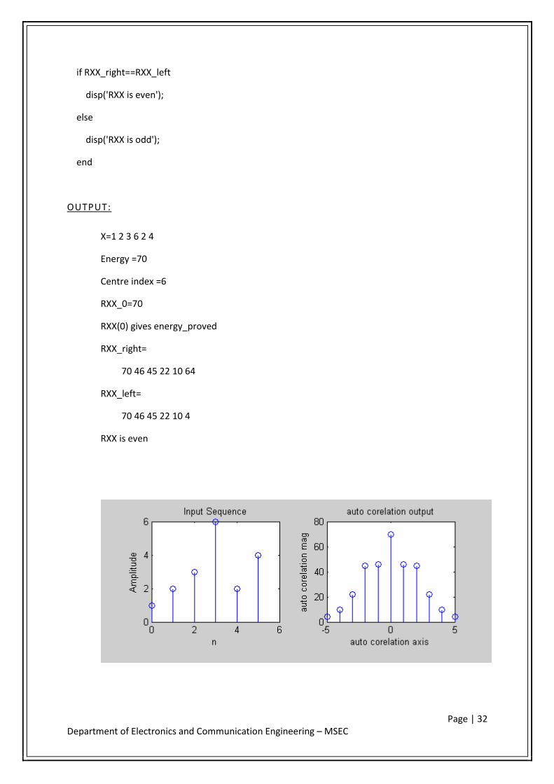
To compute the autocorrelation of the given sequence and to verify its properties
THEORY:
A mathematical operation that closely resembles convolution is correlation. Just as in the
case two signals are involved in correlation. The objective in computing the correlation between the
two signals is to measure the degree to which the signals are similar.
Suppose that we have two real sequences x(n) and y(n) each of which has finite energy. The
cross correlation of x(n) and y(n) is a sequence rxy(l), which is defined as
Where l=0, ±1, ±2…..
In the special case where y(n)=x(n), we have the autocorrelation of x(n),which is defined as
the sequence
The autocorrelation of a sequence x(n) is defined as the sequence
CALCULATIONS:
X=[1,2,3,6,2,4]
1 2 3 6 2 4
4 4 8 12 24 8 16
2 2 4 6 12 4 8
6 6 12 18 36 12 24
3 3 6 9 18 6 12
2 + 2 4 6 12 4 8
1 1 2 3 6 2 4
4 10 22 45 46 70 46 45 22 10 4
Rxx_0

Page | 30 Department of Electronics and Communication Engineering – MSEC
Property1: Energy of the signal is
E=n=-∞∑∞x[n]2=12+22+32+62+22+42=70
Rxx_n= k=-∞∑∞x(k)x(n+k)
Rxx_0= k=-∞∑∞x(k)x(k)=70
Energy =Rxx_0-------proved
Rxx(n)= k=-∞∑∞x(k)x(n+k)
X(n)=[1,2,3,6,2,4]
Put n=1
Rxx(1)= k=-∞∑∞x(k)x(1+k)
=(1*2)+(2*3)+(3*6)+(6*2)+(2*4)=46
Put n=2
Rxx(2)= k=-∞∑∞x(k)x(2+k)
=(1*3)+(2*6)+(3*2)+(6*4)=45
Put n=3
Rxx(3)= k=-∞∑∞x(k)x(3+k)
=(1*6)+(2*2)+(3*4)=22
Put n=4
Rxx(4)= k=-∞∑∞x(k)x(4+k)
=(1*2)+(2*4)=10
Put n=5
Rxx(5)= k=-∞∑∞x(k)x(5+k)
=(1*4)=4
Property2: Auto correlation output is
4 10 22 45 46 70 46 45 22 10 4
n=-5 n=0 n=5
If we fold the signal about n=0,
Rxx(n)=Rxx(-n)

Page | 31 Department of Electronics and Communication Engineering – MSEC
So even.
MATLAB CODE:
X=[1 2 3 6 2 4];
subplot(2,2,1)
n=0:1:length(X)-1;
stem(n,X);
xlabel('n');
ylabel('Amplitude');
title('Input Sequence');
RXX=Xcorr(X,X);
subplot(2,2,2)
nRXX=-length(X)+1:length(X)-1;
stem(nRXX,RXX);
xlabel('auto corelation axis');
ylabel('auto corelation mag');
title('auto corelation output');
% verification of properties
energy=sum(X.^2)
center_index=ceil(length(RXX)/2)
RXX_0=RXX(center_index)
if RXX_0==energy
disp('RXX(0) gives energy_proved');
else
disp('RXX(0) gives enegy_not proved');
end
RXX_right=RXX(center_index:1:length(RXX))
RXX_left=RXX(center_index:-1:1)
Page | 32 Department of Electronics and Communication Engineering – MSEC
if RXX_right==RXX_left
disp('RXX is even');
else
disp('RXX is odd');
end
OUTPUT:
X=1 2 3 6 2 4
Energy =70
Centre index =6
RXX_0=70
RXX(0) gives energy_proved
RXX_right=
70 46 45 22 10 64
RXX_left=
70 46 45 22 10 4
RXX is even

Page | 33 Department of Electronics and Communication Engineering – MSEC
P R O G R A M 9
TITLE:
To compute the cross correlation of the given sequence
THEORY:
Let us consider , X(t) and Y(t) are the two random processes with autocorrelation functions Rx(t,u)
and Ry(t,u), respectively. The two cross-correlation functions of X(t) and Y(t) are defined by
Rxy (t,u) = E [X(t)Y(u)]
and Ryx (t,u) = E [Y(t) X(u)]
Where t and u represent two values of times at which the processes are observed.
FEATURES OF CROSS CORRELATION FUNCTION.
1.The cross-correlation function is not generally an even function of τ
2.It does not have maximum at the origin
3.It obeys the a certain symmetry relationship indicated by following equation
Rxy(τ)=Ryx(-τ)
CALCULATIONS:
x= [1,2,4,6,5] ; y=[1,3,2,1,4]
x/y 1 2 4 6 5
1 4 8 16 24 20
3 1 2 4 6 5
2 2 4 8 12 10
1 3 6 12 18 15
4 + 1 2 4 6 5
4 9 20 35 41 31 32 21 5

Page | 34 Department of Electronics and Communication Engineering – MSEC
MATLAB CODE:
X=[1 2 4 6 5]
Y=[1 3 2 1 4]
n = 0:1:length(X)-1;
m = 0:1:length(Y)-1;
subplot(2,2,1);
stem(n,X);
xlabel('n');
ylabel('amplitude');
title('input1 sequence');
subplot(2,2,2);
stem(m,Y);
xlabel('n');
ylabel('amplitude');
title('input2 sequence');
RXY = Xcorr(X,Y)
nRXY = -length(X) +1:length(X)-1
subplot(2,2,3);
stem(nRXY,RXY);
xlabel('crosscorr axis');
ylabel('crosscorr magnitude');
title('crosscorr output');
OUTPUT:
X=1 2 4 6 5
Y=1 3 2 1 4
RXY=

Page | 35 Department of Electronics and Communication Engineering – MSEC
4.0 9.0 20.0 35.0 41.0 31.0 32.0 21.0 5.0

Page | 36 Department of Electronics and Communication Engineering – MSEC
∑
Z-1
P R O G R A M 1 0
TITLE:
Find a solution for difference equation given . Assume
initial condition as y[-1]=4, y[-2]=10
THEORY:
Family of linear time-invariant systems described by an input-output relation called a difference
equation with constant coefficients.suppose we have
A recursive system with an input-output equation
y(n) = ay(n-1)+x(n)
Where ‘a’ is constant. Figure shows a block diagram realization of the system.
X(n) Y(n)
CLACULATIONS:
Given, y[n]=x[n] +3 y[n-1]/2-y[n-2]/2
w.k.t, u[n]=1 for n>0
i) n=0:
Put n=0 in the above equation,
y[0]=x[0] +3/2 y[-1]-1/2y[-2]
y[0]=1+(3 /2)(4)-(1/2)10
y[0]=1+6-5
y[0] =2
a

Page | 37 Department of Electronics and Communication Engineering – MSEC
ii)n=1:
y[1]=x[1] +(3 /2)y[0]-(1/2)y[-1]
y[1]=1 +(3/2)(2)-4/2
y[1]=1/4+3-2
y[1]=1.25
iii)n=2:
y[2]=x[2] +(3/2) y[1]-(1/2)y[0]
y[2]=(1/4)^2 +(3/2) (1.25)-2/2
y[2]=1/16+1.875-1
y[2]=.9375
iii)n=3:
y[3]=x[3] +(3/2) y[2]-(1/2)y[1]
y[3]=(1/4) ^3 +(3/2) (.9375)-1.25/2
y[3]=.7969
iv)n=4:
y[4]=x[4] +(3/2) y[3]-y[2]/2
y[4]=(1/4) ^4+(3/2) (.7969)-.9375/2
y[4]=.7305
v)n=5:
y[5]=x[5] +(3 /2)y[4]-(1/2)y[3]
y[5]=(1/4) ^5 +(3/2) (.7305)-(1/2).7969
y[5]=.6982

Page | 38 Department of Electronics and Communication Engineering – MSEC
MATLAB CODE:
a = [1 -3/2 1/2]
b = [1]
n = 0:5;
xn=(1/4).^n;
disp('Values of x(n)');
disp(xn);
y = [4 ,10];
xic = filtic(b,a,y);
y = filter(b,a,xn,xic);
disp('The solution for difference Equation');
disp(y);
OUTPUT:
A=
1.00 -1.5 0.5
B=
1.00
Values of x(n)
1.0 0.25 0.0625 0.0156 0.0039 0.0010
The solution of equation is
1.25 0.9375 0.7969 0.7305 0.6982

Page | 39 Department of Electronics and Communication Engineering – MSEC
P R O G R A M 1 1
TITLE:
Using MATLAB design an IIR filter with passband edge frequency 1500Hz and stop band edge at
2000Hz for a sampling frequency of 8000Hz, variation of gain within pass band 1 db and stopband
attenuation of 15 db. Use Butterworth prototype design and Bilinear Transformation.
THEORY:
Butterworth filters have very smooth pass band, which we pay for with a relatively wide transition
region. A Butterworth filter is characterized by its magnitude frequency response,
| H(jΩ) | = 1 / [1+(Ω/Ωc)2N]1/2
Where, N is the order of the filter and Ωc is defined as the cutoff frequency where the filter
magnitude is 1/√2 times the dc gain (Ω=0).
Order N is given by
CALCULATIONS:
W1=(2*pi* F1 )/ Fs = 2*pi*250)/1000 =0.5∏ rad
W2=(2*pi* F2 )/ Fs = 2*pi*375)/1000 =0.75∏ rad
c 0
1
jH
21 NN
3N 32 NN

Page | 40 Department of Electronics and Communication Engineering – MSEC
Prewarp:
Ω1 = 2/T tan (w1/2) T=1sec
= 2 rad/sec
Ω2 = 2/T tan (w2/2)
= 4.8rad/sec
Order:
N = 1.956
= 2
Cut-off Frequency:
Ωc1 = Ω1 / [(10-Ap/10 - 1)](1/2n)
Ωc1 = 2
Ωc2 = Ω2 / [(10-As/10 - 1)](1/2n)
Ωc2 = 2.04
Choose Ωc = 2 rad\sec
Normalized Transfer Function:
Hn(s) = 1/[ s2 + 1.4142s + 1]
Denormalized Transfer Function:
H(s)= Hn(s) |s-s/Ωc H(s)= Hn(s) |s-s/2
H(s) = 1/[(s/2)2 + (s/2) + 1 = 4\[s2 + 2.8484s + 4]
Apply BLT:

Page | 41 Department of Electronics and Communication Engineering – MSEC
H(z) = H(s)|s=(2/T)[(1-z-1)/(1+z-1)]
MATLAB CODE:
%Butterworth Prototype
Ap=input(‘enter passband attenuation =’);
As=input(‘enter stopband attenuation =’);
fp=input(‘enter passband frequency =’);
fs= input(‘enter stopband frequency =’);
Fs=input(‘enter sampling frequency=’);
W1=2* fp / Fs ;
W2=2* fs / Fs ;
[N,Wn]=buttord(W1,W2,Ap,As)
[b,a]=butter(N,Wn)
freqz(b,a);
title(‘Butterworth frequency response’)
INPUT:
enter passband attenuation =1
enter stopband attenuation =15
enter passband frequency =1500
enter stopband frequency =2000
enter sampling frequency=8000
OUTPUT:
N =
6

Page | 42 Department of Electronics and Communication Engineering – MSEC
Wn =
0.4104
b =
0.0117 0.0699 0.1748 0.2331 0.1748 0.0699 0.0117
a =
1.0000 -1.0635 1.2005 -0.5836 0.2318 -0.0437 0.0043

Page | 43 Department of Electronics and Communication Engineering – MSEC
P R O G R A M 1 2
TITLE:
Using MATLAB design an IIR filter with passband edge frequency 1500Hz and stop band edge at
2000Hz for a sampling frequency of 8000Hz, variation of gain within pass band 1 db and stopband
attenuation of 15 db. Use Chebyshev prototype design and Bilinear Transformation.
THEORY:
A Chebyshev filter can be defined by its polynomial and its properties. A Chebyshev polynomial of
degree N is defined as,
TN(x) = cos(Ncosˉ1x),|x|≤1
cosh(Ncoshˉ1x),|x|>1.
Chebyshev polynomials can be generated using recursive formula.
TN(x) = 2 x TN-1(x) - TN-2(x), N≥2
T0(x)=1 and T1(x)=x.
There are two types of Chebyshev filters:
Chebyshev filter1 which is equiripple in the passband and monotonic in stop band. Chebyshev filter2 which is equiripple in the stopband and monotonic in passband
The properties of lowpass Chebyshev filter1 is ,
for N odd and for N even.
The filter has uniform ripples in the passband and is monotonic outside passband.
The sum of number of maxima and minima in passband equals the order of filter.
CALCULATIONS:
ω1 = (2* π * F1 )/ Fs = 2* π *100)/4000 =0.05π rad
ω2 = (2* π * F2 )/ Fs = 2* π *500)/4000 =0.25π rad
Prewarp:
Ω1 = 2/T tan (w1/2) T=1sec
= 0.157 rad/sec

Page | 44 Department of Electronics and Communication Engineering – MSEC
Ω2 = 2/T tan (w2/2)
= 0.828 rad/sec
Order:
ε = 0.765
A= 10-As/20 , A = 1020/20 , A=10
g = 13.01
Ωr= Ω2 / Ω1
Ωr=0.828/0.157 = 5.27 rad\sec
n= 1.388
Therefore, n= 2.
Cut-off Frequency:
Ωc = Ωp = Ω1 = 0.157 rad\sec
Normalized Transfer Function:
b0
= 0.505/[ s2+0.8s+0.036]
Denormalized Transfer Function:
H(s)= Hn(s) |s-s/Ωc
H(s)= Hn(s) |s-s/0.157
H(s) = 0.0125 / [s2+0.125s+0.057]

Page | 45 Department of Electronics and Communication Engineering – MSEC
Apply BLT:
H(z) = H(s)|s=(2/T)[(1-z-1)/(1+z-1)]
MATLAB CODE:
%Chebyshev Prototype
Ap=input(‘enter passband attenuation =’);
As=input(‘enter stopband attenuation =’);
fp=input(‘enter passband frequency =’);
f s= input(‘enter stopband frequency =’);
Fs=input(‘enter sampling frequency=’);
W1=2* fp / Fs ;
W2=2* fs / Fs ;
[N,Wn]=cheb1ord(W1,W2,Ap,As)
[b,a]=cheby1(N,Ap,Wn)
freqz(b,a);
title(‘Chebyshev frequency response’);
INPUT:
enter passband attenuation =1
enter stopband attenuation =15
enter passband frequency =1500
enter stopband frequency =2000
enter sampling frequency=8000

Page | 46 Department of Electronics and Communication Engineering – MSEC
OUTPUT:
N = 4
Wn = 0.3750
b = 0.0191 0.0764 0.1147 0.0764 0.0191
a = 1.0000 -1.7994 1.9637 -1.1513 0.3301

Page | 47 Department of Electronics and Communication Engineering – MSEC
P R O G R A M 1 3
TITLE:
Using MATLAB design an FIR filter to meet the following specifications choosing Hamming window:
i. Window length, N = 27
ii. Cut-off frequency = 100 Hz
iii. Sampling frequency = 1000 Hz
THEORY:
A linear-phase is required throughout the passband of the filter to preserve the shape of the given
signal in the passband. A causal IIR filter cannot give a linear-phase characteristics and only special
types of FIR filters that exhibit center symmetry in its impulse response give the linear-space. An FIR
filter with impulse response h(n) can be obtained as follows:
h(n) = hd(n) 0≤n≤N-1
= 0 otherwise ……………….(a)
The impulse response hd(n) is truncated at n = 0, since we are interested in causal FIR
Filter. It is possible to write above equation alternatively as
h(n) = hd(n)w(n) ……………….(b)
where w(n) is said to be a rectangular window defined by
w(n) = 1 0≤n≤N-1
= 0 otherwise
Taking DTFT on both the sides of equation(b), we get
H(ω) = Hd(ω)*W(ω)
Hamming window:
The impulse response of an N-term Hamming window is defined as follows:
wHam(n) = 0.54 – 0.46cos(2пn / (N-1)) 0≤n≤N-1
= 0 otherwise
CALCULATIONS:
Window length N = 27
Cutoff frequency = 100Hz
Sampling frequency = 1000Hz

Page | 48 Department of Electronics and Communication Engineering – MSEC
Centre of Symmetry / Anti-symmetry
For lowpass from FIR specifications,
hd(n) = =
desired impulse response, h(n) = hd(n) w(n)
where,
w(n) = window fun
w(n) = 0.54 – 0.46 cos ( )
MATLAB CODE:
N=input(‘Enter the window length=’);
fc=input(‘Enter cut-off frequency=’);
Fs=input(‘Enter sampling frequency=’);
Wc=2*fc/ Fs;
Wh = (hamming(N))
b = fir1(N-1, Wc ,Wh)
n hd(n) w(n) h(n)
0 0.023 0.08 1.86 x
1 0.025 0.093 2.35 x
2 0.027 0.1327 2.25 x
3 0.000 0.1957 0.00
4 0.020 0.2787 -5.7 x
5 0.037 0.3769 -0.014
6 0.0800 0.0019

Page | 49 Department of Electronics and Communication Engineering – MSEC
[h,omega] = freqz(b,1,256);
mag = 20*log10(abs(h));
plot(omega/pi,mag);
grid;
xlabel(‘Frequncy in radians in terms of pi’);
ylabel(‘gain in dB’);
title(‘Response of FIR filter using Hamming window’);
INPUT:
Enter the window length=27
Enter cut-off frequency=100
Enter sampling frequency=1000
OUTPUT:
Wh =
0.0800
0.0934
0.1327
0.1957
0.2787
0.3769
0.4846
0.5954
0.7031
0.8013
0.8843
0.9473
0.9866

Page | 50 Department of Electronics and Communication Engineering – MSEC
1.0000
0.9866
0.9473
0.8843
0.8013
0.7031
0.5954
0.4846
0.3769
0.2787
0.1957
0.1327
0.0934
0.0800
b =
Columns 1 through 6
0.0019 0.0023 0.0022 -0.0000 -0.0058 -0.0142
Columns 7 through 12
-0.0209 -0.0185 0.0000 0.0374 0.0890 0.1429
Columns 13 through 18
0.1840 0.1994 0.1840 0.1429 0.0890 0.0374
Columns 19 through 24
0.0000 -0.0185 -0.0209 -0.0142 -0.0058 -0.0000
Columns 25 through 27
0.0022 0.0023 0.0019

Page | 51 Department of Electronics and Communication Engineering – MSEC

Page | 52 Department of Electronics and Communication Engineering – MSEC

Page | 53 Department of Electronics and Communication Engineering – MSEC
G E N E R A L L A Y O U T O F C O D E C O M P O S E R S T U D I O

Page | 54 Department of Electronics and Communication Engineering – MSEC
S T E P S T O E X E C U T E A P R O G R A M U S I N G C C S
1. In the main screen go to project - - > new.. the following screen will appear .
Give a appropriate project name, project type as executable (.out) file.
Select target as TMS320C67xx (depends on the target processor we are using, in our case it’s 67xx),
and click finish in dialog box finally.

Page | 55 Department of Electronics and Communication Engineering – MSEC
2. Now a new project will be created (e.g. linear.pjt) and a tree will be displayed on left hand
side.

Page | 56 Department of Electronics and Communication Engineering – MSEC
3. Now we need to write C source code. Go to File - - > New - - > Source file.

Page | 57 Department of Electronics and Communication Engineering – MSEC
4. Now a blank screen will appear in which we have to write our C source code. Type the
source code and click save.

Page | 58 Department of Electronics and Communication Engineering – MSEC
5. We have to save the source code file as .c file. When we press save icon in main screen,
following dialog box will open. Save the file as C\C++ source file (e.g. “lin.c”).

Page | 59 Department of Electronics and Communication Engineering – MSEC
6. Now we have to add 3 files to our project.
C source code (e.g. lin.c).
A library file (e.g. rts6700.lib).
A linker command file (e.g. hello.cmd).
Firstly add the source code file.
Go to Project - - > Add files to project...

Page | 60 Department of Electronics and Communication Engineering – MSEC
Now dialog box will open ,here browse for the source code file in projects directory and and click
open .(usually the common paths are ..\ti\MyProjects\’projectname’\...)
Similarly Add two more files following same procedure .
First, add a library file from path...\ti\c6000\cgtools\lib\rts6700.lib (here file type is object
and library file).
Secondly, add a linker command file from path …\ti\tutorial\dsk6713\hello1\hello.cmd (here
the file type is linker command file *.lcf,*.cmd).

Page | 61 Department of Electronics and Communication Engineering – MSEC
7. After the addition of all three files, the expanded project tree on left hand side will resemble
this format (observe the LHS project tree which contains a library file, a source code and
linker command file.)

Page | 62 Department of Electronics and Communication Engineering – MSEC
8. Now we need to compile and build our program.
To compile go to project -- > compile file. Now the project will be compiled and any errors will be
displayed below if there.
To build go to project - - >build. Now project will be built and any errors or warnings will be
displayed below.
Page | 63 Department of Electronics and Communication Engineering – MSEC
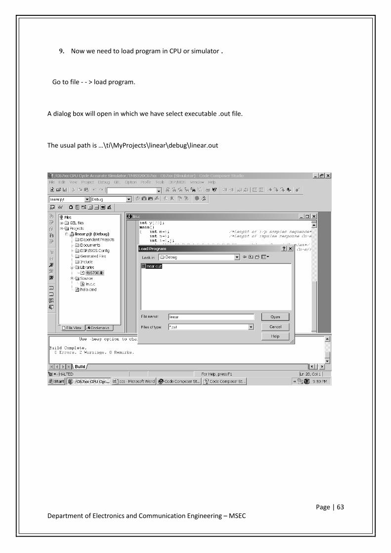
9. Now we need to load program in CPU or simulator .
Go to file - - > load program.
A dialog box will open in which we have select executable .out file.
The usual path is …\ti\MyProjects\linear\debug\linear.out

Page | 64 Department of Electronics and Communication Engineering – MSEC
10. Now we can assembly equivalent of C source code which the simulator has generated.

Page | 65 Department of Electronics and Communication Engineering – MSEC
11. To see the output of the program we have to run the program.
Go to Debug - - > Run .

Page | 66 Department of Electronics and Communication Engineering – MSEC
12. Now we can see output of the program below.
If the program needs any user input, a pop-up window will open.

Page | 67 Department of Electronics and Communication Engineering – MSEC
13. Now we need to see the plot of output .
Go to View - - > Graph - - > Time\frequency..
Now a graph property dialog box will open up.
Select Display type = single time.
Graph title = ‘Any name’.
Start address = “ the variable which we want to display”.
Index increment= 1(usually).
DSP data type = 32-bit signed integer.
DATA plot style = bar(for displaying discrete values).
Grid style = Full grid.

Page | 68 Department of Electronics and Communication Engineering – MSEC
Now the graph will be displayed as shown below:
*We can select different elements by using left and right keys of keyboard.

Page | 69 Department of Electronics and Communication Engineering – MSEC
C O D E C O M P O S E R S T U D I O P R O G R A M S
P R O G R A M 1
TITLE:
Find out the Discrete Time Convolution of the sequences x(n)=1 2 3 4 5 and h(n)=1 2 3 4, using
Code Composer Studio. Verify the results graphically.
PROGRAM:
/* program to implement linear convolution */
#include<stdio.h>
int y[20];
main()
int m=6; /*Lenght of i/p samples sequence*/
int n=6; /*Lenght of impulse response Coeff*/
int i=0,j;
int x[15]=1,2,3,4,5,6,0,0,0,0,0,0; /*Input Signal Samples*/
int h[15]=1,2,3,4,5,6,0,0,0,0,0,0; /*Impulse Response Co-efficients*/
for(i=0;i<m+n-1;i++)
y[i]=0;
for(j=0;j<=i;j++)
y[i]+=x[j]*h[i-j];
for(i=0;i<m+n-1;i++)
printf("%d\n",y[i]);
INPUT:

Page | 70 Department of Electronics and Communication Engineering – MSEC
x(n)=[1,2,3,4,5,6]
h(n)=[1,2,3,4,5,6]
OUTPUT:
y(n)=[1,4,10,20,35,56,70,76,73,60,36]

Page | 71 Department of Electronics and Communication Engineering – MSEC
P R O G R A M 2
TITLE:
Perform the Circular Convolution of the given sequence using Code Composer Studio.
PROGRAM:
/* program to implement circular convolution */
#include<stdio.h>
int m,n,x[30],h[30],y[30],i,j,temp[30],k,x2[30],a[30];
void main()
printf(" enter the length of the first sequence\n");
scanf("%d",&m);
printf(" enter the length of the second sequence\n");
scanf("%d",&n);
printf(" enter the first sequence\n");
for(i=0;i<m;i++)
scanf("%d",&x[i]);
printf(" enter the second sequence\n");
for(j=0;j<n;j++)
scanf("%d",&h[j]);
if(m-n!=0) /*If lenght of both sequences are not equal*/
if(m>n) /* Pad the smaller sequence with zero*/
for(i=n;i<m;i++)
h[i]=0;
n=m;

Page | 72 Department of Electronics and Communication Engineering – MSEC
for(i=m;i<n;i++)
x[i]=0;
m=n;
y[0]=0;
a[0]=h[0];
for(j=1;j<n;j++) /*folding h(n) to h(-n)*/
a[j]=h[n-j];
/*Circular convolution*/
for(i=0;i<n;i++)
y[0]+=x[i]*a[i];
for(k=1;k<n;k++)
y[k]=0;
/*circular shift*/
for(j=1;j<n;j++)
x2[j]=a[j-1];
x2[0]=a[n-1];
for(i=0;i<n;i++)
a[i]=x2[i];
y[k]+=x[i]*x2[i];
/*displaying the result*/
printf(" the circular convolution is\n");

Page | 73 Department of Electronics and Communication Engineering – MSEC
for(i=0;i<n;i++)
printf("%d \t",y[i]);
INPUT:
Length of first sequence = 4
Length of second sequence = 4
First sequence =[1 2 2 1 ]
Second sequence =[1 2 2 1]
OUTPUT:
The circular convolution is [9 8 9 10]

Page | 74 Department of Electronics and Communication Engineering – MSEC
P R O G R A M 3
TITLE:
Compute the response of the system whose co-efficient are a0=0.1311, a1=0.2622, a2=0.1311 and
b0=1, b1= -0.7478, b2=0.2722, when the input is a unit impulse signal.
PROGRAM:
/*program to implement impulse response of the given sequence*/
#include <stdio.h>
float y[3]=0,0,0;
float x[3]=0,0,0;
float z[10];
float impulse[10]=1,0,0,0,0,0,0,0,0,0;
main()
int j;
float a[3]=0.1311, 0.2622, 0.1311;
float b[3]=1, -0.7478, 0.2722;
for(j=0;j<10;j++)
x[0]=impulse[j];
y[0] = (a[0] *x[0]) +(a[1]* x[1] ) +(x[2]*a[2]) - (y[1]*b[1])-(y[2]*b[2]);
printf("%f\n",y[0]);
z[j]=y[0];
y[2]=y[1];
y[1]=y[0];
x[2]=x[1];
x[1] = x[0];

Page | 75 Department of Electronics and Communication Engineering – MSEC
INPUT:
Coefficient of x(n)=0.1311,0.2622,0.1311
Coefficient of y(n)=1,-0.7478,0.2722
OUTPUT:
0.131100
0.360237
0.364799
0.174741
0.031373
-0.024104
-0.026565
-0.013304
-0.002718
0.001589

Page | 76 Department of Electronics and Communication Engineering – MSEC
P R O G R A M 4
TITLE:
Compute the DFT of a sequence using code composer studio.
PROGRAM:
#include<stdio.h>
#include<math.h>
void main(void)
short N=8;
short x[8]=1,1,1,1,1,1,1,1;
float pi=3.1416;
float sumre=0, sumim=0;
float cosine=0, sine=0;
float out_real[8]=0.0, out_imag[8]=0.0;
int i=0,k=0;
for(k=0;k<N;k++)
sumre=0;
sumim=0;
for(n=0;n<N;n++)
cosine=cos(2*pi*k*n/N);
sine=sin(2*pi*k*n/N);
sumre=sumre+x[n]*cosine;
sumim=sumim-x[n]*sine;
out_real[k]=sumre;

Page | 77 Department of Electronics and Communication Engineering – MSEC
out_imag[k]=sumim;
printf("[%d]%7.3f%7.3f\n",k,out_real[k],out_imag[k]);
OUTPUT:
[0] 8.000 0.000
[1] 0.000 0.000
[2] 0.000 0.000
[3] 0.000 0.000
[4] 0.000 0.000
[5] 0.000 0.000
[6] 0.000 0.000
[7] 0.000 0.000


