
Monitoring overburden and reservoir changes from prestack time-lapse seismic data - applications to chalk fields
Thesis for the degree doktor ingeniør
Trondheim, March 2007
Norwegian University of Science and TechnologyFaculty of Engineering Science and Technology Department of Petroleum Engineering and Applied Geophysics
Thomas Røste
I n n o v a t i o n a n d C r e a t i v i t y

NTNUNorwegian University of Science and Technology
Thesis for the degree doktor ingeniør
Faculty of Natural Sciences and TechnologyDepartment of Petroleum Engineering and Applied Geophysics
© Thomas Røste
ISBN 978-82-471-0797-3 (printed version)ISBN 978-82-471-0802-4 (electronic version)ISSN 1503-8181
Doctoral theses at NTNU, 2007:37
Printed by NTNU-trykk

Abstract
Reservoir compaction due to hydrocarbon production has been observed in severalNorth Sea reservoirs, especially the chalk reservoirs in the southern part. This com-paction leads to changes in porosity and permeabilities which have implications forproduction and the production performance. In addition, reservoir compaction isoften associated with stretching and arching of the overburden rocks and subsidenceof the sea bed. The change in geomechanical stress state for the overburden rocksmight cause damage in existing wells. It is therefore of significant importance tomonitor these changes during production not only for the reservoir itself but also forthe overburden rocks. This information can be obtained from well logs; however,wells in most reservoirs are sparse and widely spread, making time-lapse seismicdata an important complementary tool.
Since compaction and stretching cause changes in both layer thickness as well asseismic velocities, it is crucial to develop methods to distinguish between the twoeffects. A new method based on detailed analysis of prestack time-lapse seismicdata is introduced to discriminate between layer thickness and velocity changes.A key parameter in this discrimination process is the dilation factor, α, which isthe relative velocity change divided by the relative thickness change within a givenlayer. This method incorporates lateral variations in relative velocity changes byutilizing zero-offset and offset-dependent time shifts.
Monitoring fault movements is important to avoid the complications associatedwith wells crossing faults that might be reactivated due to reservoir production.In addition, reactivation of overburden faults near the reservoir zone might leadto leakage of hydrocarbons and affect the reservoir drainage patterns. This thesisshows that growing faults can be obtained from prestack time-lapse seismic data.A growing fault tip appears as a distortion pattern with characteristic time shiftversus offset signatures. From raypath considerations and modeling, the positionand vertical extent of a distortion zone can be determined. The distortion patternsdisappear if the time-lapse data is stacked, meaning that prestack data containscrucial information. The correlation between a time-lapse distortion zone and agrowing fault tip is investigated on high quality prestack time-lapse seismic oceanbottom cable (OBC) data from the Valhall Field. A compacting reservoir zone
iii

exists directly beneath this fault tip, validating that a growing fault might causethe observed anomalies. Growing faults complicate the interpretation of time-lapsedata since large vertical (in addition to lateral) variations in thickness and velocitychanges occur. This thesis presents an extended method to estimate the dilationfactor (α) in such cases. This method can be viewed as a simplified version oftime-lapse tomography, but involving fewer unknown parameters, giving more sta-bility to the estimated changes in thickness and velocity. In addition, the presentedmethod is faster and cheaper than a full tomographic method.
In many reservoirs, 30-40% of the oil reserves remain unproduced. To identifyundrained areas and detect drainage patterns, it is crucial to monitor the reservoirchanges during production. Reservoir monitoring leads to saved costs due to re-duced number of misplaced wells and increased production because of optimizedwell planning. From time-lapse amplitude variation with offset (AVO) analysis,it is possible to estimate reservoir pressure and saturation changes. This thesisintroduces a new method which also includes compacting reservoirs. This is ini-tially a three-parameter problem, including pressure and saturation changes andcompaction. However, from laboratory measurements, the reservoir compaction isrelated to the pressure and saturation changes. Using an empirical relation betweenporosity, saturation, and pressure changes, the problem is reduced to involve onlythe pressure and saturation changes, which can be solved from time-lapse AVOanalysis.
iv

Acknowledgments
I am forever grateful to my supervisor, Professor Martin Landrø, for all help andrecommendation. His knowledge and experience has been of great inspiration. To-gether with good humor, he has encouraged and motivated me during the thesiswriting.
Acknowledgments go to TOTAL for financial support, and Jerome Guilbot, YahuiYin, and Ruben Sanchez for valuable discussions. I also want to thank the peopleat TOTAL for several pleasant stays at TOTAL, Pau and TOTAL, Stavanger. AlanBurns, Ottar Minsaas, Ole J. Nydal, Hilde Skeie, and Jon Kleppe are acknowledgedfor interesting meetings between TOTAL and NTNU.
I want to thank Shell, Rijswijk, as well as Paul Hatchell and Peter Wills, for alleffort and support spent to make the article given in chapter 4 possible. The helpand discussions with the people at Shell, Rijswijk have been very useful, and thecollaboration with Paul Hatchell will be remembered.
The Valhall partnership (BP Norge AS, Amerada Hess Norge AS, A/S Norske Shelland Total E&P Norge AS) are acknowledged for permission to publish the articlesgiven in chapters 3 and 4, as well as Ole Jøran Askim, Olav Barkved, and Tron G.Kristiansen for support and discussions.
Thanks to post doc. Alexey Stovas for fruitful discussions and for the collabo-ration during the work of the article given in chapter 3. Thanks to Øyvind Kvamfor advises in the first years of my thesis work and for help regarding finite differencemodeling. All my friends and colleagues at the Department of Petroleum Engineer-ing and Applied Geophysics are acknowledged for support and discussions, not onlyrelated to this thesis, but also for topics which made life easier through 4 years ofhard work. I will particularly mention Ørjan Pedersen, Tor Erik Rabben, SverreJohnsen, Christian Crescente, Sissel Martinsen, Egil Tjaland, Janniche Nordskag,Andre Strupstad, Alf Lackner, Olve Rasmussen, Amir Ghaderi, Rune Holt, Ken-neth Duffaut, and Andreas Evensen.
I acknowledge inspiration from all speed skating friends, especially Arne-Kjell Fold-
v

vik for his enthusiasm regarding this thesis.
I want to thank my parents for all support and encouragement through many yearsof study. This work has been impossible without them.
Special thanks go to my girlfriend, Tone, for her patience during my travels abroadand late night working. She always motivated me not to give up, even in the difficultperiods where an ending of this thesis seemed impossible.
vi

Contents
Abstract iii
Acknowledgments v
1 Thesis Introduction 11.1 Motivation for the thesis . . . . . . . . . . . . . . . . . . . . . . . . 11.2 Linking geomechanics and time-lapse seismic . . . . . . . . . . . . . 31.3 Reservoir changes and time-lapse seismic . . . . . . . . . . . . . . . 41.4 The Valhall Field . . . . . . . . . . . . . . . . . . . . . . . . . . . . 51.5 Thesis content . . . . . . . . . . . . . . . . . . . . . . . . . . . . . . 7
2 Background theory 112.1 The wave equation . . . . . . . . . . . . . . . . . . . . . . . . . . . 112.2 Sedimentary rocks . . . . . . . . . . . . . . . . . . . . . . . . . . . 142.3 Rock physics models . . . . . . . . . . . . . . . . . . . . . . . . . . 15
2.3.1 A pack of uniform spheres . . . . . . . . . . . . . . . . . . . 152.3.2 Velocity-porosity relations with bounds . . . . . . . . . . . . 152.3.3 Critical porosity model . . . . . . . . . . . . . . . . . . . . . 182.3.4 Empirical velocity-porosity relations . . . . . . . . . . . . . . 20
2.4 Determining α from porosity-velocity relations . . . . . . . . . . . . 22
3 Estimation of layer thickness and velocity changes using 4D prestackseismic data 253.1 Abstract . . . . . . . . . . . . . . . . . . . . . . . . . . . . . . . . . 253.2 Introduction . . . . . . . . . . . . . . . . . . . . . . . . . . . . . . . 263.3 Methodology . . . . . . . . . . . . . . . . . . . . . . . . . . . . . . 28
3.3.1 Estimating α based on time shift analysis . . . . . . . . . . 283.3.2 Uncertainty analysis . . . . . . . . . . . . . . . . . . . . . . 31
3.4 Synthetic example . . . . . . . . . . . . . . . . . . . . . . . . . . . 323.4.1 The 2D synthetic model . . . . . . . . . . . . . . . . . . . . 323.4.2 Description of the survey . . . . . . . . . . . . . . . . . . . . 363.4.3 Synthetic results . . . . . . . . . . . . . . . . . . . . . . . . 36
3.5 Field-data example . . . . . . . . . . . . . . . . . . . . . . . . . . . 41
vii

viii CONTENTS
3.5.1 Estimating α for the overburden . . . . . . . . . . . . . . . . 433.5.2 Estimating α for the reservoir layer and overburden rocks . . 483.5.3 Anisotropy . . . . . . . . . . . . . . . . . . . . . . . . . . . . 51
3.6 Discussion . . . . . . . . . . . . . . . . . . . . . . . . . . . . . . . . 523.7 Conclusions . . . . . . . . . . . . . . . . . . . . . . . . . . . . . . . 533.8 Acknowledgments . . . . . . . . . . . . . . . . . . . . . . . . . . . . 543.A Rock physics . . . . . . . . . . . . . . . . . . . . . . . . . . . . . . 553.B Detailed derivation of the method . . . . . . . . . . . . . . . . . . . 563.C Testing equation (3.9) for a two-layer model . . . . . . . . . . . . . 593.D Uncertainty estimates . . . . . . . . . . . . . . . . . . . . . . . . . . 603.E Synthetic model parameters . . . . . . . . . . . . . . . . . . . . . . 633.F Uncertainty in estimated α . . . . . . . . . . . . . . . . . . . . . . . 65
4 Monitoring overburden layer changes and fault movements fromtime-lapse seismic data on the Valhall Field 674.1 Abstract . . . . . . . . . . . . . . . . . . . . . . . . . . . . . . . . . 674.2 Introduction . . . . . . . . . . . . . . . . . . . . . . . . . . . . . . . 684.3 Discrimination between layer thickness and velocity changes . . . . 714.4 Estimate α from permanent OBC data . . . . . . . . . . . . . . . . 734.5 Time-lapse distortions . . . . . . . . . . . . . . . . . . . . . . . . . 854.6 Discussion . . . . . . . . . . . . . . . . . . . . . . . . . . . . . . . . 944.7 Conclusions . . . . . . . . . . . . . . . . . . . . . . . . . . . . . . . 964.8 Acknowledgments . . . . . . . . . . . . . . . . . . . . . . . . . . . . 974.A Detailed derivation of the method . . . . . . . . . . . . . . . . . . . 984.B Extended method . . . . . . . . . . . . . . . . . . . . . . . . . . . . 101
5 Estimation of layer thickness and velocity changes in anisotropicrocks 1035.1 Abstract . . . . . . . . . . . . . . . . . . . . . . . . . . . . . . . . . 1035.2 Introduction . . . . . . . . . . . . . . . . . . . . . . . . . . . . . . . 1035.3 Estimating α for rocks undergoing time-lapse changes in anisotropy 105
5.3.1 Synthetic examples for time-lapse anisotropy changes . . . . 1075.4 Discussion . . . . . . . . . . . . . . . . . . . . . . . . . . . . . . . . 1145.5 Conclusions . . . . . . . . . . . . . . . . . . . . . . . . . . . . . . . 1145.A Detailed derivation of the method . . . . . . . . . . . . . . . . . . . 116
6 Discrimination between pressure and fluid saturation changes incompacting reservoirs from time-lapse seismic data 1216.1 Abstract . . . . . . . . . . . . . . . . . . . . . . . . . . . . . . . . . 1216.2 Introduction . . . . . . . . . . . . . . . . . . . . . . . . . . . . . . . 1226.3 Saturation and stress versus seismic parameters . . . . . . . . . . . 123
6.3.1 Using PP-reflectivity changes . . . . . . . . . . . . . . . . . 133

ix
6.4 Synthetic data example . . . . . . . . . . . . . . . . . . . . . . . . . 1356.5 Discussion . . . . . . . . . . . . . . . . . . . . . . . . . . . . . . . . 1376.6 Conclusions . . . . . . . . . . . . . . . . . . . . . . . . . . . . . . . 1406.7 Acknowledgments . . . . . . . . . . . . . . . . . . . . . . . . . . . . 1416.A The inversion procedure . . . . . . . . . . . . . . . . . . . . . . . . 1426.B Synthetic models undergoing overburden changes . . . . . . . . . . 1446.C Using PP and PS time shifts . . . . . . . . . . . . . . . . . . . . . . 145
7 Closing remarks 147
References 149

x CONTENTS

Chapter 1
Thesis Introduction
Monitoring reservoir and overburden changes during hydrocarbon production is im-portant to identify undrained areas and for planning placement of wells. Repeated(time-lapse) seismic data is important to obtain this information. The objective ofthis thesis is to improve the understanding of time-lapse seismic data analysis ofcompacting hydrocarbon fields. I introduce new methods based on prestack time-lapse seismic data analysis to monitor production-induced reservoir changes andassociated overburden changes. Production-induced compaction of reservoir rockshas been observed in several North Sea reservoirs, especially chalk reservoirs likeValhall and Ekofisk (in the southern part of the North Sea). Reservoir compactionleads to changes in porosity and permeabilities which have implications for produc-tion and the production performance. In addition, reservoir compaction is oftenassociated with stretching of the overburden rocks. The change in geomechanicalstress state for the overburden rocks might lead to damage in existing wells. It istherefore of great interest to the industry to monitor both overburden and reservoirchanges during production.
1.1 Motivation for the thesis
Reservoirs producing oil or gas are subjected to pore pressure depletion. This cre-ates changes in the stress and strain fields of the rock material both inside andoutside the reservoir. For reservoir rocks with high compressibility, such as chalksand unconsolidated sands, pressure depletion leads to compaction, which has im-plications for production by changing permeabilities and, hence, the productionperformance (Hall et al., 2005).
Reservoir compaction due to hydrocarbon production has been observed in severalNorth Sea reservoirs, especially the chalk reservoirs in the southern part. Guilbotand Smith (2002) utilized time isochron differences from 4D seismic data to detectcompaction and subsidence at the Ekofisk Field. They observed seismic time shifts
1

2 Motivation for the thesis
up to 12-16 ms between 1989 and 1999, related to compaction values of up to 6 mfor the reservoir chalk formation.
In many reservoirs, compaction of the reservoir rocks represents the major drivemechanism. Significant volumes of produced hydrocarbons may be credited to thiseffect. However, compaction may also lead to subsidence of the sea bed. At theValhall Field, Barkved and Kristiansen (2005) report a maximum subsidence of thesea bed larger than 5.4 m (since the field came on production in 1982) and increas-ing by 0.25 m per year. At the Ekofisk Field, the extensive compaction resultedin sea bed subsidence of nearly 8 m by 2000 (Chin and Nagel, 2004). It is typicalfor these fields that the sea bed subsidence is less than the corresponding reservoircompaction, meaning that the overburden rocks are stretched. Often the changein geomechanical stress state for the overburden rocks leads to damage in existingwells (especially when significant shear stresses are introduced as a byproduct ofthe reservoir compaction). It is therefore of importance to map the velocity andthickness changes during production not only for the reservoir itself, but also forthe overburden rocks. Time-lapse seismic data can be utilized to obtain this infor-mation.
Reservoir compaction may also lead to movements of faults. Several authors (Ewing,1985; White and Morton, 1997; Morton et al., 2006) discuss the coupling betweenreservoir compaction and slip along growth faults that become active when suffi-ciently large volumes of fluid (oil, gas, or formation water) are produced. Reynoldset al. (2003) determined the relative attendant risk of reactivation of faults in theBight Basin by evaluating the in situ stress field. Mildren et al. (2002) studied re-activation of faults by using the FAST (Fault Analysis Seal Technology) technique.Monitoring fault movements is important for several reasons. Reactivation of faultsmight lead to leakage of hydrocarbons and affect the reservoir drainage patterns.Fault seal breach in the North Sea (Gaarenstroom et al., 1993), the Penola Through(Jones et al., 2000), and the Gulf of Mexico (Finkbeiner et al., 2001) have been re-lated to faulting and fracturing associated with the in situ stress. Based on seismicdata and wellbore information, Allan diagrams (Allan, 1989) are often used to iden-tify potential petroleum leak points along a fault strike. In addition to leakage ofhydrocarbons, hazards are associated with wells crossing reactivated faults (Alsoset al., 2002). Barkved et al. (2003) report a strong correlation between overburdenfaults and drilling problems at the Valhall Field. Maury et al. (1992) discuss fur-ther how slipping faults can pose serious problems in the field since it may causecasing failure. Reactivated faults can also have close relationship with earthquakes.Zoback and Zinke (2002) recorded numerous microearthquakes at the Valhall Fieldduring a six week monitoring period. They found the microearthquakes consistentwith a normal faulting stress regime.

Thesis Introduction 3
Monitoring reservoir and overburden layer changes and movements of faults is there-fore important, and the combined use of time-lapse seismic data and geomechanicalknowledge is expected to be important in future monitoring projects.
1.2 Linking geomechanics and time-lapse seismic
Several authors (Rhett, 1998; Chin et al., 2002; Vikram and Settari, 2005) havecreated geomechanical and fluid flow models of compacting reservoirs based on lab-oratory studies of reservoir rocks. Minkoff et al. (2004) try to predict productionin compacting reservoirs by linking geomechanics and flow models with time-lapseseismic. Hatchell et al. (2005) and Vidal et al. (2002) try to integrate time-lapseseismic and geomechanics to characterize reservoir changes. Hatchell and Bourne(2005a) constructed forward models of time-lapse time shifts from stress and strainfields using geomechanical models and a stress/strain-dependent seismic velocity.They found that a simple linear model relating seismic velocity with vertical normalstrain works well for several locations around the world.
It is important to notice that time-lapse time shifts capture the combined effects ofvelocity and thickness changes within a given layer. For a layer undergoing thick-ness changes, the seismic velocity is altered by the changes in the stress and strainfields. For a layer of thickness, z, I express the relative time shift in terms of therelative thickness change and velocity change as (Landrø and Stammeijer, 2004;Hatchell and Bourne, 2005b; Røste et al., 2005)
∆T0
T0≈ ∆z
z− ∆v
v, (1.1)
where T0 represents seismic two-way vertical traveltime within the layer and v isthe layer velocity. The notations ∆T0, ∆z, and ∆v represent changes in verticaltwo-way traveltime, thickness, and velocity, respectively. (Note that the relativethickness change ∆z/z is identical to the average vertical strain εzz over the layer.)A major challenge for quantitative time-lapse analysis is to discriminate betweenthickness changes and velocity changes for both the reservoir section and the over-burden. Landrø and Janssen (2002) presented a method utilizing near and far offsettraveltime shifts to perform this discrimination procedure.
As a first order approximation for a relation between relative thickness and ve-locity changes for a given subsurface layer it might be reasonable to assume thatthe two changes are proportional to each other:
∆v
v≈ α
∆z
z, (1.2)

4 Reservoir changes and time-lapse seismic
where the ”dilation factor” α < 0 is a parameter dependent on the rock properties ofthe layer. This is a crucial parameter, since it determines the ratio between velocityand thickness changes. The knowledge of the dilation factor from a rock physicspoint of view is limited; there are no measurements available to my knowledge. Ido not know if the dilation factor is the same for compaction and stretching of arock. Furthermore, the dilation factor might also be dependent on the magnitude ofthe relative thickness change. Despite these concerns, I find it fruitful to introducethe dilation factor, since it captures the important relation between velocity andthickness changes. Furthermore, as later shown in section 2.4, the dilation factorcan easily be determined from empirical porosity-velocity relations, e.g. given byMavko et al. (1998).
1.3 Reservoir changes and time-lapse seismic
Hydrocarbon production will cause pore pressure and fluid saturation changes. Bothpressure and saturation changes might influence time-lapse seismic data (Landrø,1999), and it is often difficult to separate the two effects based on stacked PP time-lapse data only. In many time-lapse seismic studies, seismic differences between abaseline and a monitor survey are analyzed as either a pressure effect (Watts etal., 1996) or a fluid effect (Landrø et al., 1999; Gabriels et al., 1999). However,for some fields or segments within the field, both fluid and pressure changes haveapproximately the same degree of impact on the seismic data. In such cases the useof time-lapse amplitude variation with offset (AVO) analysis (see Tura and Lumley,1998, 1999a; Landrø, 1999; Landrø, 2001) or time-lapse PP- and PS-reflectivitystacks (see Landrø et al., 2003; Stovas et al., 2003) offer an opportunity to discrim-inate between the two effects. However, these methods do not include reservoircompaction; that is, porosity changes are neglected. Modifications are thereforeneeded for reservoirs where production or water injection induces porosity changes.
At first, one might assume that changes in saturation, pressure, and porosity arethree independent parameters. However, from laboratory measurements of chalkSylte et al. (1999) found that porosity changes are related to saturation and pres-sure changes; that is, the pressure changes might induce fractures and compactionof the weak chalk matrix, while water has a weakening effect on chalk. The rela-tion between porosity changes (∆φ), saturation changes (∆Sw), and effective stresschanges (∆σ) can be given as (Sylte et al., 1999)
∆φ =∂φ
∂σ∆σ +
∂φ
∂Sw∆Sw, (1.3)
where ∂φ/∂σ and ∂φ/∂Sw are partial differentiations of the porosity with respectto stress and water saturation, respectively.

Thesis Introduction 5
In addition to reservoir stress and saturation changes, time-lapse seismic data mightbe influenced by other effects, such as changes in temperature. Variations in reser-voir temperature are usually small. However, cases where temperature changesmight occur are when steam (temperature around 300◦C) is injected in a shallowreservoir with temperature between 10-30◦C (e.g. the Duri Field, Jenkins et al.,1997), or when cold sea water (temperature 0-15◦C) is injected into deeper reser-voirs with temperature 70-90◦C (Jack, 1997). Such temperature changes mightchange both velocity and density (Mavko et al., 1998; Batzle and Wang, 1992).
1.4 The Valhall Field
The methods proposed in this thesis are mainly tested on prestack time-lapse seis-mic data from the Valhall Field, situated in the southern part of the NorwegianNorth Sea (see Figure 1.1). The Valhall Field is an over-pressured Late Cretaceouschalk reservoir. The field was discovered in 1975 (after exploration drilling in the
Figure 1.1: Location of the Valhall Field in the Norwegian sector of the NorthSea (Barkved et al., 2003).

6 The Valhall Field
period 1969-1974) and started producing in October 1982. Daily production is onthe order of 100 000 barrels of light oil (Barkved and Kristiansen, 2005). Thereservoir layer is at depth 2500 m and ranges in thickness from 0-70 m. Porosityis 35-50% and matrix permeability is generally low, less than 10 mD. Palaeoceneshale provides the cap rock. The water depth is 70 m.
The expected recovery rate in 1982 was 14%, a figure which has now increasedto 40% (Barkved and Kristiansen, 2005). Time-lapse seismic monitoring with highquality in addition to improved methods to interpret and utilize the seismic mightincrease the recovery further. The seismic response is very sensitive to production-induced features (such as reservoir compaction, depletion, stretched overburdenlayers, and seabed subsidence). This was first demonstrated by marine streamerdata, acquired in 1992 and 2002. Figure 1.2 shows time-lapse seismic data from thesouth-east part of the Valhall Field (from 1992 and 2002). Large pull-down effects
Figure 1.2: Time-lapse seismic data from the south-east part of the Valhall Field,acquired in 1992 and 2002. Large time shifts and amplitude changes are observednear the reservoir zone.

Thesis Introduction 7
and amplitude changes are observed at the top and base of the reservoir layer. Thetime-lapse seismic effects are mainly due to compaction of the reservoir (inducedby the pore pressure decrease and fluid saturation changes during hydrocarbon pro-duction).
In 2003, a permanent ocean bottom cable (OBC) array was installed at the ValhallField, initiating the ”Life of Field Seismic” (LoFS) program which includes a seriesof 3D OBC surveys. The first survey was acquired from September to November2003 with subsequent surveys acquired in intervals of approximately 4 months. Re-sults from the earliest surveys confirm that the system can provide high qualitydata with good repeatability (Kommedal et al., 2004; Barkved, 2004).
In January 2004, water injection started in the center of the field. Field and lab ob-servations indicate that water has a weakening effect on the reservoir chalk. For theEkofisk chalk field, this water-weakening phenomenon became the primary mech-anism for reservoir compaction in 1993, 6 years after the start of water injection(Sylte et al., 1999). Reservoir compaction due to water weakening is also expectedat the Valhall Field.
1.5 Thesis content
The thesis contains 7 chapters, including this introduction. The chapters 3, 4, and6 represent independent papers.
This introductory chapter 1 states the motivation for the thesis. The challengesregarding geomechanical changes during hydrocarbon production are mentioned.Also included is a short description of the Valhall Field.
Chapter 2 contains background theory, including a derivation of the wave equa-tion. Several rock physics models are discussed. By assuming uniaxial stress-strainrelations, the dilation factor α is determined based on porosity-velocity relations.
Chapter 3 introduces a new method which discriminates between velocity and thick-ness changes of stretched or compacted rocks. The method is based on detailedanalysis of time-lapse prestack seismic data, and incorporates lateral variations in(relative) velocity changes by utilizing zero-offset and offset-dependent time shifts.The method is tested on a 2D synthetic model that undergoes severe reservoircompaction as well as stretching of the overburden rocks. Finally, the method isutilized to analyze a real 2D prestack time-lapse seismic line from the Valhall Field,acquired in 1992 and 2002. The authors of this paper are T. Røste, A. Stovas,and M. Landrø. The paper was published in the November-December 2006 issue of

8 Thesis content
Geophysics (Røste et al., 2006). The work has been presented at the 67th EAGEConference & Exhibition in Madrid, Spain, June 2005, at the ROSE meeting inTrondheim, Norway, June 2005, and at the FORCE seminar in Stavanger, Norway,September 2005.
In chapter 4, time-lapse changes are investigated on prestack time-lapse seismicocean bottom cable (OBC) data from LoFS survey 1 and survey 3. The OBCrecording system provides data with high quality and good repeatability. By uti-lizing the method introduced in chapter 3, changes in thickness and velocity areestimated for a sequence from the sea bed to the top reservoir horizon. In addition,time-lapse time shift distortion patterns that move systematically with offset areobserved. We show that one of the distortion zones (observed between LoFS sur-vey 1 and 3) correlates with buried faults, indicating that a (time-lapse) distortionzone might be produced by a localized slip in a fault zone. An extended methodis introduced to describe such positions. The authors of this paper are T. Røste,M. Landrø, and P. Hatchell. The paper was submitted to Geophysical Journal In-ternational in May 2006 and accepted for publication in January 2007. In April2006, the paper was presented at the ROSE meeting in Trondheim, Norway and inJanuary 2007, an expanded abstract was submitted to the 69th EAGE Conference& Exhibition.
The time-lapse discrimination method discussed in chapters 3 and 4 is developed forisotropic cases. However, the earth is most probably anisotropic, and an isotropiccase is only a simplified description of the earth. Chapter 5 describes an extendeddiscrimination method which accounts for time-lapse anisotropy changes. Approx-imations regarding the included anisotropy were necessary to avoid large, complexterms. The method is tested on synthetic anisotropic models undergoing differ-ent scenarios of thickness, velocity, and anisotropy changes. Compared with theisotropic method, the proposed method produces better results for the anisotropictime-lapse datasets. For cases with static anisotropy, the derived method becomesidentical to the isotropic method.
Chapter 6 introduces a method which discriminates between pressure and fluidsaturation changes in compacting reservoirs. The proposed method is based ontime-lapse amplitude variation with offset (AVO) analysis. Based on laboratorymeasurements, the reservoir compaction (or porosity loss) is related to the pressureand saturation changes. By using this empirical relation, explicit expressions forcomputing pressure- and saturation-related changes from time-lapse seismic dataare obtained. The method is tested on synthetic models with different productionscenarios. The authors of this paper are T. Røste and M. Landrø. In January 2007,an expanded abstract of this work was submitted to the 69th EAGE Conference &Exhibition.

Thesis Introduction 9
Finally, chapter 7 completes the thesis with closing remarks.

10

Chapter 2
Background theory
2.1 The wave equation
Seismic sound waves can be viewed as subsurface disturbances that propagate withvelocities given by the elastic stiffness and the density of the rock. Seismic waves in-duce elastic deformation along the propagation path in the subsurface. The equationof wave propagation in elastic solids is derived by using Hooke’s law and Newton’ssecond law of motion. Most rocks have an ability to resist and recover from thedeformations produced by forces. This ability is called elasticity. When an elasticmaterial is subjected to stresses, changes in shape and dimensions occur. Thesechanges are referred to as strains. Fjær et al. (1992) evaluate in detail how rockmaterials respond to a dynamic, time harmonic external stress (or strain).
Strain is defined as the relative change in a dimension or shape of a body. It iscommon to discriminate between normal strains, shearing strains, and rotations.Normal strains are related to volumetric changes, shearing strains are related toangular deformations, and rotations occur without any deformations. Adding to-gether the normal strains in the x-, y-, and z-direction of a Cartesian coordinatesystem, gives the relative change in volume, ∆ (Sheriff and Geldart, 1995):
∆ = εxx + εyy + εzz, (2.1)
where εxx, εyy, and εzz denote the relative change in length in x-, y-, and z-direction(respectively) of the material.
Hooke’s law states that for small volumetric changes, a given strain is directlyproportional to the stress producing it. The strains involved in seismic waves areusually less than 10−8 (except very near the source), which validates the use ofHooke’s law. When several stresses exist, each produces strains independently ofthe others. This means that each strain is a linear function of all of the stressesand vice versa. In general, Hooke’s law leads to complicated relations between
11

12 The wave equation
strain and stress. But for an isotropic medium, Hooke’s law can be expressed inthe following relatively simple form (Love, 1944; Timoshenko and Goodier, 1934):
σii = λ∆ + 2µεii, i = x, y, z, (2.2)
σij = 2µεij , i, j = x, y, z; i �= j, (2.3)
where the parameters λ and µ (Lame’s constants) denote elastic stiffness and shearmodulus, respectively. Equations (2.2) and (2.3) represent the stress-strain relationsfor normal components and shear components, respectively, and are often expressedas a matrix equation, σ = Cε:⎡
⎢⎢⎢⎢⎢⎢⎣
σxx
σyy
σzz
σxy
σyz
σzx
⎤⎥⎥⎥⎥⎥⎥⎦
=
⎡⎢⎢⎢⎢⎢⎢⎣
λ + 2µ λ λ 0 0 0λ λ + 2µ λ 0 0 0λ λ λ + 2µ 0 0 00 0 0 µ 0 00 0 0 0 µ 00 0 0 0 0 µ
⎤⎥⎥⎥⎥⎥⎥⎦
⎡⎢⎢⎢⎢⎢⎢⎣
εxx
εyy
εzz
εxy
εyz
εzx
⎤⎥⎥⎥⎥⎥⎥⎦
. (2.4)
Acoustic wave propagation can be described by Newton’s second law of motion.The unbalanced force acting on a small volume element of rock equals the masstimes the acceleration. In the x-direction, this gives the equation of motion on thefollowing form:
ρ∂2u
∂t2=
∂σxx
∂x+
∂σxy
∂y+
∂σxz
∂z, (2.5)
where u is the particle displacement in the x-direction, ρ is the density, and t denotestime. Substituting Hooke’s law into equation (2.5) gives an equation expressing thedisplacement (in x-direction) in terms of strains (e.g. Sheriff and Geldart, 1995):
ρ∂2u
∂t2= (λ + µ)
∂∆
∂x+ µ∇2u, (2.6)
where ∇2u is the Laplacian of u; that is, ∇2u = ∂2u/∂x2 + ∂2u/∂y2 + ∂2u/∂z2.Similar equations can be found for the motion along the y- and z-axis. Addingtogether the equations for motion in x-, y-, and z-direction gives the well-knownwave equation:
ρ∂2∆
∂t2= (λ + 2µ)∇2∆. (2.7)
The Lame constant λ can be related to other elastic constants, e.g. λ = K − 23µ,
where K and µ denote bulk and shear moduli, respectively. Using this relationgives the wave equation on following form:
ρ∂2∆
∂t2= (K +
4
3µ)∇2∆, (2.8)

Background theory 13
which is the most common representation. If the wave propagation is parallel tothe displacement u; that is, a longitudinal (or compressional) wave, equation (2.8)reduces to
vP =
√K + 4
3µ
ρ, (2.9)
where vP denotes the velocity of a compressional or primary wave. For a mode ofmotion in which the particles are displaced only in the x-direction, and the wavepropagation is only in the y-direction, equation (2.8) becomes
vS =
õ
ρ. (2.10)
The subscript S denotes that this is a shear wave. The combined particle and wavemotion of compressional and shear waves are illustrated in Figure 2.1. Equations(2.9) and (2.10) show that vP is always larger than vS. For a fluid media
vP =
√K
ρ, vS = 0, (2.11)
since no shear forces exist.
The relation between velocity (vP or vS), elastic moduli (K, µ), and density (ρ)appears to be straightforward from equations (2.9) and (2.10). However, this isnot the case since K, µ, and ρ are also related to other characteristics of the rock.
Direction ofwave propagation
�
P-wave � � � � � � � � � � �
S-wave� �
��
� � ��
�� �
Figure 2.1: Particle motion of P-wave and S-wave propagation (slightly modifiedfrom Fjær et al., 1992).

14 Sedimentary rocks
These characteristics may be material and structure of the rock, type or lithology,porosity, degree of fluid saturation, pressure, depth, cementation, degree of com-paction, etc. The most notable inhomogeneity of sedimentary rocks is that they areporous and filled with fluid. Wang and Nur (1992) discuss theories relating seismicvelocity to the composition of rocks.
2.2 Sedimentary rocks
Sedimentary rocks (sandstones, limestones, shales, etc.) can be considered as packedgrains. The space between the grains is called the pore space. This pore space isfilled with fluid; that is, oil, water, or gas. Pore pressure is the fluid pressure inthe pore space. For a case with perfect communication between the pores, the porepressure is equal to the hydrostatic pressure caused by the weight of the fluid. Thepore pressure at depth z can then be expressed as
pf (z) =
∫ z
z0
ρf (z)gzdz + pf (z0), (2.12)
where ρf (z) is the fluid density at depth z and g is the gravitational constant.The pressure at depth z0, denoted pf (z0), is usually the atmospheric pressure. Hy-drostatic pressure is often referred to as normal pressure conditions. Rocks thatdeviate from the hydrostatic pressure are either called overpressured or underpres-sured, depending on whether the pressure is greater or less than the normal pressure.
The overburden pressure is defined as the combined weight of sediments and fluidoverlying a formation:
P (z) =
∫ z
z0
ρ(z)gzdz, (2.13)
whereρ(z) = φ(z)ρf + (1 − φ(z))ρS. (2.14)
The parameters ρf and ρS denote the fluid and solid densities and φ is the porosity.The difference between the pore fluid pressure (pf ) and the overburden pressure(P ) is called the effective stress (σ):
σ = P − ηpf , (2.15)
where η is the Biot coefficient. For static compression of the rock frame, the Biotcoefficient is defined as (Mavko et al., 1998)
η = 1 − Kfr
KS, (2.16)
where Kfr and KS are the bulk and solid moduli of the frame, respectively. Forsoft materials, η ≈ 1.

Background theory 15
2.3 Rock physics models
Rock physics models that relate velocity and impedance to porosity and mineralogyform a critical part of seismic analysis for porosity and lithofacies. Illustrations ofvelocity-porosity relations are given by Mavko et al. (1998) and Avseth et al.(2005).
2.3.1 A pack of uniform spheres
The simplest rock model consists of identical spheres arranged in a cubic pattern.The porosity of such a model is 0.48 (that is, 1 − π/6) and the average density canbe estimated to π/6 times the density of the material of the spheres. Based onTimoshenko and Goodier (1951), the effective elastic modulus K can be related tothe compressive pressure and elastic constants of the spheres.
Gassmann (1951) calculated the velocity for a hexagonal packing of identical spheresunder a pressure produced by the overburden spheres. The cubic and hexagonalpacked spheres give the same variation of velocity with depth. This velocity vari-ation with depth is also consistent with Faust (1953), which found an empiricalformula for velocity in terms of depth of burial and formation resistivity. However,individual measurements of the velocity at a given depth deviate largely betweenthese formulas. This is due to the fact that the porosity estimations are inaccurate(Sheriff and Geldart, 1995).
Random packs of well-sorted particles have porosities in the range of 0.4-0.5, butunder pressure, the particles deform at the points of contact, and as a result thedensity increases and the porosity decreases. Clearly, porosity is an important fac-tor controlling velocities. In addition, the velocity is dependent of fluid in the pores,which affect the density as well as the effective elasticity of the rock.
2.3.2 Velocity-porosity relations with bounds
A useful velocity-porosity relation can be provided by upper and lower bounds onthe elastic moduli of rocks. Specifying the volume fractions of the constituentsand their elastic moduli, without any geometric details of their arrangement, it ispossible to predict the upper and lower bounds on the moduli and velocities of thecomposite rock.
The simplest bounds are the Voigt (1910) and Reuss (1929) bounds. The Voigtupper bound on the effective elastic modulus MV of a mixture of N material phases

16 Rock physics models
is given as (Mavko et al., 1998)
MV =N∑
i=1
fiMi, (2.17)
where fi and Mi are the volume fraction and elastic modulus, respectively, of thei-th constituent. The Voigt upper bound (also called isostrain average) representsthe elastically stiffest rock that nature can put together. The Reuss lower bound(also called isostress average) of the effective elastic modulus MR is
1
MR=
N∑i=1
fi
Mi, (2.18)
which represents the elastically softest rock that nature can put together. Thevariable M in the Voigt and Reuss formulas can represent any modulus. However,it is most common to compute Voigt and Reuss averages of the bulk modulusM = K and shear modulus M = µ. Figure 2.2 shows an illustration of Voigtand Reuss bounds for the bulk modulus K for a mixture of two constituents. Theconstituents might be two different minerals or a mineral plus fluid (water, oil, orgas). A well-known example where the Reuss model gives a correct prediction is asuspension of particles in a fluid. The undrained bulk modulus K of the suspensionis given by
1
K=
φ
Kfluid+
1 − φ
Ksolid, (2.19)
where Kfluid and Ksolid are the bulk moduli of the fluid and the solid mineral ma-terial, respectively, and φ is the porosity. Equation (2.19) is also known as Wood’s(1941) equation.
The best bounds, in the sense of giving the narrowest possible range of elasticmoduli without specifying anything about the geometries of the constituents, arethe Hashin-Shtrikman bounds (Hashin and Shtrikman, 1963). For a mixture of twoconstituents, the Hashin and Shtrikman bounds are given by (Mavko et al., 1998)
KHS± = K1 +f2
(K2 − K1)−1 + f1(K1 + 43µ1)−1
, (2.20)
µHS± = µ1 +f2
(µ2 − µ1)−1 + 2f1(K1+2µ1)
5µ1(K1+43µ1)
, (2.21)
where the two individual phases of the bulk modulus K, shear modulus µ, and vol-ume fractions f are denoted with subscripts 1 and 2. Upper and lower bounds arecomputed by interchanging which material is subscripted 1 and which is subscripted

Background theory 17
KV
KR
KV : Voigt upper bound
KR
: Reuss lower bound
StifferSofter
Volume fraction of material 2
Effe
ctiv
e bu
lk m
odul
us
0 1
Figure 2.2: Illustration of the Voigt upper and Reuss lower bounds on the effectivebulk modulus of a mixture of two constituents (modified from Mavko et al., 1998).
2. Generally, the expressions give the upper bound when the stiffest material is sub-scripted 1 in the expressions above, and the lower bound when the softest materialis subscripted 1.
The physical interpretation of the bounds for bulk modulus is shown schemati-cally in Figure 2.3. The space is filled by an assembly of spheres of material 2, eachsurrounded by a shell of material 1. Each sphere and its shell has exactly the volumefractions f1 and f2. The upper bound is obtained when the stiffer material formsthe shell; the lower bound is obtained when it is in the core. A more general formof the Hashin-Shtrikman bounds, which can be applied to more than two phases, isdiscussed by Mavko et al. (1998).
The separation between the upper and lower bounds of Voigt-Reuss and Hashin-Shtrikman depends on the difference in elasticity of the constituents. For mixedsolids that are elastically similar, the bounds are fairly close. In such cases, asimple assumption for predicting the effective medium is the Hill’s (1963) average,which is the average of the upper and lower bounds; that is, KHill = (K+ +K−)/2.

18 Rock physics models
Figure 2.3: Physical interpretation of the Hashin-Shtrikman bounds for bulk mod-ulus of a two-phase material (slightly modified from Mavko et al., 1998): An as-sembly of spheres of material 2, each surrounded by a shell of material 1.
However, when the constituents are quite different (for example minerals and porefluids), the bounds become quite separated, and the prediction is more difficult.
2.3.3 Critical porosity model
Sedimentary rocks form initially as unconsolidated deposits of gravels, sand, or mud(see e.g. Boggs, 2001). Before deposition, sediments exist as particles in suspen-sion. Newly deposited sediments are characterized by loosely packed, uncementedfabrics; high porosities; and high interstitial water content. The porosity of newlydeposited sediments is referred to as the critical porosity φc (Nur, 1992). When theporosity gets below the limiting φc, the grains start to carry load. Porosity may de-crease further during diagenesis, which is the final stage of forming conglomerates,sandstones, and shales (Boggs, 2001). Figure 2.4 illustrates the different stages inthe process of forming sedimentary rocks.
Nur et al. (1995) presented a simple method that separates the mechanical andacoustic behavior of porous materials into two distinct domains separated by thecritical porosity φc. In the suspension domain; that is, φ > φc, the effective bulk andshear moduli are quite accurately described by the Reuss average given in equation(2.18). In the load-bearing domain; that is, φ < φc, the frame (or dry) bulk and

Background theory 19
Fluid−Supported
Suspension
Diagenesis
0 1
Frame−Supported
Quartz Sandstone Sand
Porosity
φc
Figure 2.4: Different stages in the process of forming sedimentary rocks (slightlymodified from Nur et al., 1998). The critical porosity φc is defined as the porosityof newly deposited sediments.
shear moduli can be expressed as the linear functions
Kfr = KS
(1 − φ
φc
), (2.22)
µfr = µS
(1 − φ
φc
), (2.23)
where KS and µS are the solid bulk and shear moduli, respectively. Figure 2.5shows bulk modulus (K/KS) versus porosity for a water saturated rock, accordingto Nur’s critical porosity model, Voigt-Reuss bounds, Voigt-Reuss-Hill, and HashinShtrikman bounds. An empirical curve (dotted line) for clean sandstones, measuredby Murphy et al. (1993), is included for comparison.
The weakness of the critical porosity model is that the critical porosity is not anuniversal constant (not even for a given class of rock, such as sandstones). Thestrength is the simplicity: no other assumptions about the microstructure than theknowledge of critical porosity are needed.
The loosest possible packing of spherical, equally sized grains is simple cubic packingwhich gives a porosity of 0.48, while random loose packing gives porosities between0.4 and 0.45. For clean, well sorted sands, the critical porosity is near 0.4. Chalkhas pores that are most likely spherical in shape, leading to critical porosity as highas 0.6-0.7.
Figure 2.6 shows P-wave velocity versus porosity for a variety of water-saturated

20 Rock physics models
0 0.1 0.2 0.3 0.4 0.5 0.6 0.70
0.1
0.2
0.3
0.4
0.5
0.6
0.7
0.8
0.9
1
Porosity
K/K
s Voigt
HS+
HillReuss = HS−
Criticalporosity
Voigt
HS+
Reuss = HS−
Criticalporosity
Figure 2.5: Bulk modulus versus porosity for a water-saturated rock, according tovarious models (solid lines). For comparison, an empirical curve for clean sandstones(Murphy et al., 1993) is included (dotted line).
sediments, ranging from ocean-bottom suspensions to consolidated sandstones. Thedata is compared with Voigt and Reuss bounds computed for mixtures of quartzand water. In the porosity domain above the critical porosity, sediments follow theReuss average of mineral and fluid (that is, the undrained bulk modulus K is givenby equation (2.19)). Below the critical porosity, the touching grains will induceeffective stress, compaction, and cementing, which lead the sediments off the Reussbound. In this porosity domain, the rock properties follow steep trajectories start-ing at the critical porosity and ending at the mineral end point at zero porosity(Figure 2.6). These trends are often described by empirical relations.
2.3.4 Empirical velocity-porosity relations
Porosity has an enormous impact on P- and S-wave velocities. Several authors (e.g.Wyllie et al., 1956; Raymer et al., 1980; Tosaya and Nur, 1982; and Han et al.,1986) have derived empirical relations for velocity versus porosity in the porositydomain below critical porosity.

Background theory 21
1000
2000
3000
4000
5000
6000
0 0.2 0.4 0.6 0.8 1.0
suspensionssand–clay mixturesand
clay-free sandstone clay-bearing sandstone
P-ve
loci
ty (m
/s)
Porosity
Voigt avg.
Reuss bound
Suspensions
Newly deposited clean sand
Processes that give sediment strength: compaction, stress, diagenesis
Figure 2.6: P-wave velocity versus porosity for a variety of water-saturated sedi-ments (Avseth et al., 2005). The data is compared with the Voigt-Reuss bounds.
Wyllie et al. (1956) introduced a relation that is still commonly used in the oilindustry. For a fluid-saturated rock with high effective pressure, they found thefollowing relation between P-wave velocity vP and porosity φ:
1
vP
=φ
vP,f
+1 − φ
vP,s
, (2.24)
where vP,s and vP,f are the P-wave velocities of the solid and fluid, respectively.The interpretation of equation (2.24) is that the sound wave shares its time passingthrough the rock in a volumetric portion in the solid and pore fluid. This is strictlyvalid only if the wavelength is much shorter than the grain and pore size; that is,for high frequencies. Improvements of Wyllie’s empirical formula are suggested by

22 Determining α from porosity-velocity relations
Raymer et al. (1980).
Han et al. (1986) show that velocity-porosity relations are dependent on the claycontent. These relations are obtained from ultrasonic measurements of sandstoneswith porosities, φ, ranging from 0.03 to 0.3 and clay volume fractions, C , rangingfrom 0 to 0.55. For an effective pressure of 40 MPa, Han’s velocity-porosity relationfor a water-saturated shaley sandstone reads
vP = (5.59 − 2.18C) − 6.93φ, (2.25)
vS = (3.52 − 1.89C) − 4.91φ, (2.26)
where vP and vS are given in km/s. Equations (2.25) and (2.26) indicate parallelvelocity-porosity trends with zero-porosity intercepts dependent on the clay content.
Tosaya and Nur (1982) determined similar trends based on other ultrasonic mea-surements of velocity, porosity, and clay content. For water-saturated rocks at aneffective pressure of 40 MPa, they obtained the following relation:
vP = (5.8 − 2.4C) − 8.6φ, (2.27)
vS = (3.7 − 2.1C) − 6.3φ, (2.28)
where φ is porosity, and C is the clay content. Similar empirical regressions arealso found by Castagna et al. (1985). Klimentos (1991) obtained relations betweenvelocity, porosity, clay content, and permeability.
2.4 Determining α from porosity-velocity relations
The dilation factor α (that is, the relative thickness change divided by the relativevelocity change within a given layer) can be determined from empirical porosity-velocity relations e.g. given by Mavko et al. (1998). If the seismic velocity issome function of porosity, v(φ), where ∆v/∆φ = v′(φ), the α-value can be foundby assuming uniaxial stress-strain relations. For a porous material with uniaxialstress-strain relations (e.g. Guilbot and Smith, 2002), the change in thickness isrelated to the change in porosity approximately as ∆z/z ≈ ∆φ/(1− φ). This givesthe following relation between the velocity change and thickness change (comparewith Hatchell and Bourne, 2005a):
∆v
v= (1 − φ)
v′(φ)
v(φ)
∆z
z, (2.29)
and, hence,
α = (1 − φ)v′(φ)
v(φ). (2.30)

Background theory 23
For rocks with linear relations between porosity and velocity; that is, v = a − bφ,where a and b are positive constants, α can be given as (Appendix 3.A):
α =a − b
v− 1. (2.31)
As an example, using Tosaya’s empirical porosity-velocity relation, given by equa-tion (2.27), I find the following for clean sandstones:
v = 5.8 − 8.6φ, (2.32)
α =5.8 − 8.6
5.8 − 8.6φ− 1, (2.33)
giving α = −1.7 for a sandstone with porosity 0.20. Figure 2.7 shows estimatedα versus porosity for the rock physics models given by Han (equation (2.25)) andTosaya and Nur (equation (2.27)). The estimations are based on clean sandstones(solid lines) and sandstones with clay content 0.5 (dashed lines). (See Hatchell andBourne (2005a) for further estimations based on rock-properties trends.) Figure 2.7shows that the dilation factor α increases in magnitude as the clay content increases.Note, however, that this result gives the same dilation factor for a compacting rockand a stretching rock. In comparison, Hatchell and Bourne (2005a) found that αis larger in absolute value for rock elongation (stretch) than for rock contraction(compaction) for several locations around the world. They estimate α-values around−5 for rocks undergoing elongation strains and α-values ranging from −1 to −3 forrocks undergoing contraction. Different α-values for stretched overburden rocks andcompacted reservoir rocks is also predicted by Røste et al. (2006) at the ValhallField.

24 Determining α from porosity-velocity relations
0 0.05 0.1 0.15 0.2 0.25 0.3
−5
−4
−3
−2
−1
0
Porosity
α−va
lue
Han, clean sandstoneHan, clay = 0.5Tosaya, clean sandstoneTosaya, clay = 0.5
Figure 2.7: Estimated α versus porosity based on Han’s and Tosaya’s empiricalvelocity-porosity relations for clean sandstones and sandstones with clay content of0.5.

Chapter 3
Estimation of layer thickness andvelocity changes using 4Dprestack seismic data
Thomas Røste*, Alexey Stovas*, and Martin Landrø*
*Norwegian University of Science and Technology,Department of Petroleum Engineering and Applied Geophysics,S.P.Andersens vei 15A, N-7491 Trondheim, Norway.
Published in the November-December 2006 issue of Geophysics. Presented at the67th EAGE Conference & Exhibition in Madrid, Spain, June 2005, at the ROSEmeeting in Trondheim, Norway, June 2005, and at the FORCE seminar in Sta-vanger, Norway, September 2005.
3.1 Abstract
In some hydrocarbon reservoirs severe compaction of the reservoir rocks is observed.This compaction is caused by production, and is often associated with stretchingand arching of the overburden rocks. Time-lapse seismic data can be used to mon-itor these processes. Since compaction and stretching cause changes in both layerthickness as well as seismic velocities, it is crucial to develop methods to distinguishbetween the two effects.
We introduce a new method based on detailed analysis of time-lapse prestack seis-mic data. The equations are derived assuming that the entire model consists of
25

26 Introduction
only one single layer with no vertical velocity variations. The method incorporateslateral variations in (relative) velocity changes by utilizing zero-offset and offset-dependent time shifts. To test the method, we design a 2D synthetic model thatundergoes severe reservoir compaction as well as stretching of the overburden rocks.Finally, we utilize the method to analyze a real 2D prestack time-lapse seismic linefrom the Valhall Field, acquired in 1992 and 2002. For a horizon at a depth ofaround 2.5 km, which is near the top reservoir horizon, a subsidence of 2.7 m and avelocity decrease of 4.5 m/s for the sequence from the sea surface to the top reservoirhorizon are estimated. By assuming that the base of the reservoir remains constantin depth, a reservoir compaction of 3.6 % (corresponding to a subsidence of the topreservoir horizon of 2.7 m), and a corresponding reservoir velocity increase of 6.7 %(corresponding to a velocity increase of 200 m/s), are estimated.
3.2 Introduction
Production-related compaction has been observed in several North Sea reservoirs,especially the chalk reservoirs in the southern part. For example, the compactionof the Valhall Field, at 2.5 km depth, has led to 4.5 m of subsidence at the sea bedsince the field came on production in 1982 (Pattillo et al., 1998). Such reservoircompaction will have significant implications for production by changing perme-abilities and, hence, the production performance (Hall et al., 2005). It is typicalfor these fields that the sea bed subsidence is less than the corresponding reservoircompaction, meaning that the overburden rocks are stretched. Often the change ingeomechanical stress state for the overburden rocks might lead to damage in exist-ing wells (especially when significant shear stresses are introduced as byproduct ofthe reservoir compaction). It is therefore of significant importance to map the ve-locity and thickness changes during production not only for the reservoir itself, butalso for the overburden rocks. Between the wells, time-lapse seismic data is a com-plementary tool for obtaining this information, and the combined use of repeatedseismic measurements and geomechanical knowledge is expected to be important infuture monitoring projects.
Guilbot and Smith (2002) utilized time-isochron differences from 4D seismic datato detect compaction and subsidence at the Ekofisk Field. They observed seismictime shifts up to 12-16 ms between 1989 and 1999, related to compaction valuesof up to 6 m for the reservoir chalk formation. They used a 4D tomographic tech-nique where the nonuniqueness between velocity and thickness changes was solvedby introducing a velocity-porosity relationship for the reservoir chalk layer. It isimportant to notice that the 4D time shifts capture the combined effects of velocityand thickness changes within a given layer. For a layer of thickness, z, we expressthe relative time shift in terms of the relative thickness change and velocity change

Estimation of layer thickness and velocity changes using 4D prestack seismic data 27
as (Landrø and Stammeijer, 2004; Hatchell and Bourne, 2005b; Røste et al., 2005)
∆T0(x0)
T0(x0)≈ ∆z(x0)
z(x0)− ∆v(x0)
v(x0), (3.1)
where T0 represents seismic two-way vertical traveltime within the layer and v is thelayer velocity. The parameter x0 denotes the global x-coordinate for a given CDP-location (position), and ∆T0, ∆z, and ∆v represent changes in vertical two-waytraveltime, thickness, and velocity, respectively. A major challenge for quantita-tive time-lapse analysis is to discriminate between thickness changes and velocitychanges for both the reservoir section and the overburden. Landrø and Janssen(2002) presented a method utilizing near and far offset traveltime shifts to performthis discrimination procedure. In this paper we introduce a prestack method whichutilizes all offsets. As a first order approximation for a relation between relativethickness and velocity changes for a given subsurface layer we will simply assumethat the two changes are proportional to each other (Røste et al., 2005):
∆v(x0)
v(x0)≈ α
∆z(x0)
z(x0), (3.2)
where the ”dilation factor” α is a parameter dependent on the rock propertiesof the layer. This is a crucial parameter, since it determines the ratio betweenvelocity and thickness changes. In general, α varies with spatial coordinates. It isimportant to stress that the knowledge of the dilation factor from a rock physicspoint of view is limited; there are no measurements available to our knowledge. Wedo not know if the dilation factor is the same for compaction and stretching of arock. Furthermore, the dilation factor might also be dependent on the magnitude ofthe relative thickness change. Despite these concerns, we find it fruitful to introducethe dilation factor, since it captures the important relation between velocity andthickness changes. Furthermore, it can easily be determined if empirical porosity-velocity relations are available. Assuming uniaxial stress-strain relations and alinear relation between porosity (φ) and velocity (v); that is, v = a − bφ, it can beshown (Appendix 3.A) that α is given by
α =a − b
v− 1. (3.3)
Note that α ≤ 0 because, by equation (3.A-1)), v ≥ a − b. From equation (3.3) itis clear that α is rock (and lithology) dependent. However, in this paper, we willassume that α is constant for the sequence of layers we study.
Using the empirical relations for the chalk reservoir at Valhall we obtain a valuefor the dilation factor of −1.5. If we use the empirical porosity-velocity relationpublished by Tosaya and Nur (1982) we find an α-value of −2.4 for sand and −3.6

28 Methodology
for clay. Han’s (1986) relation gives an α-value equal to −1.6 for sand and −2.7 forclay. These observations indicate that rocks with high clay content will have dilationfactors that are larger in magnitude than clean sands and chalks. (However, notethat Han’s relation is only based on consolidated sandstones, not unconsolidatedsands or shales.)
In the following sections we introduce a method which estimates changes in layerthickness and velocity based on prestack time-lapse seismic data. The developedmethod is tested on a 2D synthetic model which consists of 7 layers, including ananticline reservoir section. Both the reservoir layer and the overburden layers (ofthe synthetic model) undergo changes in layer thickness and velocity that vary withlateral position. Finally, we test the method on a 2D prestack time-lapse seismicline from the Valhall Field.
3.3 Methodology
To discriminate between layer thickness and velocity changes, defined by the dilationfactor α, both zero-offset and offset-dependent time shifts are utilized. From raypathconsiderations we include lateral variations in layer changes, which is normally thecase for both the reservoir layer and overburden layers when the reservoir undergoesstrong compaction.
3.3.1 Estimating α based on time shift analysis
Assume a prestack CDP-gather at position x0. The seismic two-way traveltime for araypath with offset 2h can be expressed as an integral over the total raypath lengthS,
T (x0, h) =
∫S
ds
v(s), (3.4)
where v(s) denotes the P-wave velocity at the ray position s(x0, h). Assume a one-layer model with a P-wave velocity field, v(x), that varies along the lateral positionx, but is nonvarying with depth (Figure 3.1). By assuming straight raypaths, it canbe shown that (similar to assuming average slowness within the offset range 2h)
T (x0, h) =
√1 +
z2(x0)
h2
x0+h∫x0−h
dx
v(x), (3.5)
where z(x0) represents the layer thickness at the CDP-position x0. The straightraypath assumption used above will lead to inaccuracies, so this equation should beused with care if the variations in velocity are significant and heterogeneous. Equa-tion (3.5) describes the initial (or pre-production) case. For the post-production

Estimation of layer thickness and velocity changes using 4D prestack seismic data 29
v(x)ds z
hx0
Figure 3.1: Sketch showing that we assume straight raypaths in a model withlateral variations in velocity.
case, we find that it is essential to include the lateral variations in velocity changes,since it is very likely that such changes will occur both within the reservoir layeras well as the overburden layers of a producing hydrocarbon reservoir. It is alsopossible to include vertical variations in velocity changes. This essentially meansthat we approach time-lapse tomography (Vesnaver et al., 2003). However, the ideaof this paper is to develop something simpler than a full tomographic method, andwe therefore assume no vertical variations in velocity changes. From equation (3.5)the two-way prestack traveltime for the monitor case (for a one-layer model) is thengiven as
T′(x0, h) =
√1 +
z2(x0)
h2
(1 +
∆z(x0)
z(x0)
)2x0+h∫
x0−h
dx
v(x)(1 + ∆v(x)
v(x)
) , (3.6)
where the relative change in velocity, ∆v(x)/v(x), might vary laterally but not withdepth. (Note that variations in thickness changes only affect the multiplier outsidethe integral in equation (3.6) when assuming straight raypaths.) Assuming smallrelative changes in velocity and thickness, the relative change in two-way traveltimebecomes (see Appendix 3.B)
∆T (x0, h)
T (x0, h)≈
(1 + z2(x0)
z2(x0)+h2∆z(x0)z(x0)
) x0+h∫x0−h
dxv(x)
(1 − ∆v(x)
v(x)
)x0+h∫x0−h
dxv(x)
− 1. (3.7)

30 Methodology
From equations (3.1) and (3.2) the relative changes in layer thickness and velocitycan be related to the relative change in two-way vertical traveltime T0:
∆z(x0)
z(x0)≈(
1
1 − α
)∆T0(x0)
T0(x0),
∆v(x0)
v(x0)≈(
α
1 − α
)∆T0(x0)
T0(x0). (3.8)
By assuming small lateral variations in initial layer velocity in the vicinity of eachposition x0; that is, v(x) ≈ v(x0) for x0 − h ≤ x ≤ x0 + h, equation (3.7) canbe written in the simple form given by equation (3.9) (see Appendix 3.B). Note,however, that we include the lateral variations in ∆v; that is, ∆v = ∆v(x).
∆T (x0, h)
T (x0, h)≈ z2(x0)
z2(x0) + h2
(1
1 − α
)∆T0(x0)
T0(x0)− 1
2h
(α
1 − α
) x0+h∫x0−h
dx∆T0(x)
T0(x). (3.9)
The relative change in two-way traveltime (for a given half-offset h) is therefore de-pendent on α and the estimated relative change in vertical traveltime. (Note thatthe integration sign in equation (3.9) in practice means summation, since time shiftestimations only exist for discrete positions (or CDPs).) The parameter α is deter-mined by minimizing the least square error in relative traveltime change (equation(3.9)) over the entire offset range. This α-value is then inserted into equation (3.8)to obtain the changes in layer thickness and velocity.
Equation (3.9) is only valid for one layer. However, equation (3.9) might be appliedfor a sequence of layers if the relative velocity changes (captured by the relativezero offset time shifts inside the integral sign in equation (3.9)) have no verticalvariations. Further, due to the assumption made for equation (3.2), α must be sim-ilar for the layers within the investigated sequence. However, choosing a sequenceconsisting of layers that undergo similar processes, for example, an overburden se-quence that only undergoes stretch, we believe that the vertical variations in therelative velocity changes are less important than the lateral variations. For a two-layer model, it is possible to estimate the relative traveltime shift as a function ofoffset (Appendix 3.C). A comparison between the two-layer traveltime shift and thetraveltime shift estimated using equation (3.9) is shown in Figure 3.2. This exampleshows that the one-layer approximation given by equation (3.9) can be used if theprecautions listed above are taken into account. In addition, for stretched over-burden rocks, Hatchell and Bourne (2005a) find α to be almost constant (around−5) for several worldwide field examples. Equation (3.9) might therefore be testedon an overburden sequence that only undergoes stretch. When applying equation(3.9) to a sequence of layers, we find that the inaccuracies increase with increasedvariations in (relative) velocity changes between the layers.
When both vertical and horizontal variations in velocity changes are significantand appear to be heterogeneous, a full 4D tomographic approach is required.

Estimation of layer thickness and velocity changes using 4D prestack seismic data 31
3.3.2 Uncertainty analysis
The method is strongly influenced by how accurately we can measure zero-offsetand offset-dependent time shifts from time-lapse seismic data. In addition, largesensitivity in α is needed to be able to discriminate the correct α-value; that is, atest of various values of α (for a given position) should give clearly distinct results(from equation (3.9)). (This is later discussed for results from synthetic and fielddata). Errors due to the approximations made from equation (3.6) to equation (3.9)are given step by step in Appendix 3.D.
0 0.5 1 1.5 2 2.5 3 3.5 42.5
3
3.5
4
4.5
5
Max deviation: 3.3 %
Offset (km)
∆T /
T (
10−3
)
Figure 3.2: Comparison between computed relative traveltime shifts for a two-layer model (solid line) and equation (3.9) (dashed line). A maximum error of 3.3%is observed at 4.0 km offset. Initial thickness of each layer is 1.0 km, velocity offirst layer is 1.8 km/s and second layer velocity is 2.5 km/s. The dilation factorα is −4 for both layers, and the stretching of the two layers are 0.6 m and 1.0 m,respectively.

32 Synthetic example
3.4 Synthetic example
3.4.1 The 2D synthetic model
The described method is tested on a 2D synthetic model with a total depth of 3.5km and a total lateral size of 16 km (Figure 3.3). The model consists of 7 layersincluding an anticline-shaped reservoir section with thickness (pre-production) givenas (all units in km)
zres = −5.600 × 10−3x2 + 8.960 × 10⁻²x − 0.2184. (3.10)
The reservoir thickness (equation (3.10)) varies from zero at position x = 3 km to140 m at the crest (x = 8 km) to zero again at x = 13 km. P-wave velocity (vp),S-wave velocity (vs), and density (ρ) for all 7 layers (pre-production) are given inTable 3.1 (layer 1 is the water layer). The reservoir velocity (vp = 2900 m/s and vs
= 1500 m/s) yields a vp/vs-ratio similar to oil-bearing chalk (that is, vp/vs = 1.9 -2.0).
Inside the compacting area (5.5 km < x < 10.5 km) the thickness change of thereservoir, ∆zres, varies from zero at position x = 5.5 km to −10 m at the crest(x = 8 km) to zero again at x = 10.5 km. The polynomial expression (effective onlyinside the compacting area 5.5 km < x < 10.5 km) reads (all units in km)
∆zres = 1.600 × 10−3x2 − 2.560 × 10⁻²x + 9.240 × 10⁻², (3.11)
where negative ∆zres corresponds to reservoir compaction. The reservoir thicknesschanges (equation (3.11)) are shown in bottom of Figure 3.4 together with a plotof the reservoir after compaction (top).
Table 3.1: Initial layer P-wave velocities (vp), S-wave velocities (vs), and densities(ρ) used in the synthetic model. Layer 1 denotes the water layer and layer 6 denotesthe reservoir layer.
Layer vp (m/s) vs (m/s) ρ (g/cm3)1 1476 0 1.002 1700 800 1.553 1800 900 1.604 2000 1000 1.705 2200 1200 1.756 2900 1500 1.807 4000 2500 2.30

Estimation of layer thickness and velocity changes using 4D prestack seismic data 33
Changes in reservoir thickness can be linked to changes in other reservoir param-eters (such as changes in porosity, velocity, and density). Empirical relationshipsbetween reservoir velocity (vp,res, vs,res) and porosity (φres) have previously been used(Guilbot and Smith, 2002) to estimate reservoir compaction. Here we adapt thesame technique to establish our forward compaction model. For a chalk reservoir itis reasonable to assume
vp,res = a − bφres , vs,res = a′ − b′φres, (3.12)
where
a = 5500 m/s , b = 7000 m/s , a′ = 2845 m/s , b′ = 3621 m/s. (3.13)
0 2 4 6 8 10 12 14 16
0
0.5
1
1.5
2
2.5
3
3.5
2D synthetic model
Layer 2
Layer 3
Layer 4
Layer 5
Res
Layer 7
Assume changesonly in this area
Position, x (km)
Dep
th, z
(km
)
Figure 3.3: The initial (pre-production) 7-layer synthetic model, given in kilome-ters. Changes are assumed to occur only in the area between the vertical dashedlines; that is, between the positions 5.5 km and 10.5 km.

34 Synthetic example
0 2 4 6 8 10 12 14 16
2.5
2.6
2.7
2.8
2.9
3
Position, x (km)
Dep
th, z
(km
)
0 2 4 6 8 10 12 14 16
−15
−10
−5
0
5
Position, x (km)
∆z (
m)
Figure 3.4: The compacted reservoir section of the synthetic model (top) afterapplying the thickness changes plotted at bottom. Both figures plotted as a functionof position.
The above parameters are estimated from well logs. We assume that the reservoirdensity follows the relation:
ρres = φresρF + (1 − φres)ρS , (3.14)
where ρF and ρS are the fluid and solid densities of the reservoir, respectively. Byassuming uniaxial strain conditions, differentiation of equations 3.12 and 3.14 reads(see Appendix 3.E)
∆vp,res = −b(1 − φres)∆zres
zres + ∆zres, (3.15)
∆vs,res = −b′(1 − φres)∆zres
zres + ∆zres
, (3.16)
Estimation of layer thickness and velocity changes using 4D prestack seismic data 35
∆ρres = −(ρres − ρF )∆zres
zres + ∆zres
, (3.17)
where we (still for the forward model) use the following reservoir parameters: poros-ity φres = 0.37, fluid density ρF = 0.8 g/cm
3, and reservoir density ρres = 1.8 g/cm
3.
Note that ∆vp,res, ∆vs,res, and ∆ρres vary laterally since zres and ∆zres (given byequations 3.10 and 3.11, respectively) vary laterally. The maximum ∆vp,res (at thecrest, position x = 8 km) is 339 m/s, found from equation (3.15) by substitutingthe maximum reservoir thickness (zres = 140 m) and thickness change (∆zres = −10m). This gives (equation (3.2))
αres ≈ ∆vp,res
vp,res
(∆zres
zres
)−1
=339 m/s
2900 m/s
(−10 m
140 m
)−1
= −1.6, (3.18)
for the crest. Further estimations by equation (3.2) show that αres varies with posi-tion between −1.4 and −1.6. (Note also that αres can be found exactly by equation(3.3), which gives (constant) αres = a−b
vp,res− 1 = −1.5).
For the forward model the thickness changes (or stretch) of an overburden layeri, denoted ∆zi, are directly linked to the reservoir compaction; see Appendix 3.E.The relative changes in P- and S-wave velocities of an overburden layer i (belowthe sea bed) are given by
∆vp,i
vp,i=
∆vs,i
vs,i= −2 × ∆zi
zi, (3.19)
which means that we assume α = −2 within each of the overburden layers (belowthe sea bed) for the synthetic case. When looking at the total overburden sequencefrom the sea surface to the top reservoir horizon the modeled α-value is obtainedfrom equation (3.2). For the crest (position x = 8 km) we get
αoverb ≈ ∆Voverb
Voverb
(∆zoverb
zoverb
)−1
=−4.95 m/s
1888.4 m/s
(10 m
2660 m
)−1
= −0.7, (3.20)
where zoverb and ∆zoverb denote the thickness and thickness change (at the crest) ofthe total overburden sequence, respectively. Note that the estimated αoverb = −0.7(for the total overburden sequence) is independent of the subsidence of the sea bed,meaning that the thickness change, ∆zoverb, is simply equal to the subsidence of thetop reservoir horizon. This leads to the different α-value for the total overburdensequence (−0.7) and the individual overburden layers (−2). The relative change invertical velocity (at the crest of the given overburden sequence), ∆Voverb/Voverb, areobtained from the Dix interval velocity (Sheriff and Geldart, 1995). Substitutingvalues for other positions in equation (3.20) show that αoverb varies with position,between −0.69 and −0.72.

36 Synthetic example
Assuming that the mass within each layer is conserved, and that the stretch onlyoccurs in the z-direction, the relative changes in density can approximately be givenas (see Appendix 3.E)
∆ρi
ρi
≈ −∆zi
zi
. (3.21)
Note also that the overburden layer changes ∆vp,i, ∆vs,i, and ∆ρi vary laterallysince ∆zi is linked to ∆zres (see more details in Appendix 3.E).
3.4.2 Description of the survey
The prestack time-lapse seismic data were modeled by a 2D coarse grid finite dif-ference scheme (Yerneni et al., 2002). A Ricker wavelet with central frequency of23 Hz was used. The temporal step-length was 1 ms and the grid size was 4 m by4 m. The receiver cable consisted of 300 receivers with a spacing of 12.5 m. Thedistance between the source and the first receiver was 150 m, and the shot pointinterval was 25 m. Based on the synthetic time-lapse seismic data, traveltime shiftsfor all offsets were estimated.
3.4.3 Synthetic results
Prior to estimating traveltimes of events in a prestack gather we mute all signalsabove and below the selected events; see Figure 3.5. Traveltimes are then pickedfor interpolated maximum amplitude. Zero offset traveltimes (T0) are estimated byassuming that the picked traveltimes (T ) follow standard hyperbolic moveout (Dix,1955); that is,
T 2(x0, h) = T 20 (x0) +
4
V 2rms(x0)
h2, (3.22)
where h denotes half-offset and Vrms denotes rms velocity. For a given position x0,the picked traveltimes are interpolated along a straight line in the h2-T 2-domain,according to equation (3.22), to obtain T0 (and Vrms). For the synthetic model wehave investigated the overburden sequence from the sea surface to the top reservoirhorizon (for both baseline and monitor). Figure 3.6 shows the estimated (crosses)and lateral smoothed (solid line) relative time shifts for zero offset for the inves-tigated sequence (for positions inside the compacting area, 5.5 km - 10.5 km),together with the modeled values (dashed line). The thickness (pre-production) ofthe investigated sequence, given by
z(x0) ≈ T0(x0)Vrms(x0)
2, (3.23)
is necessary input to equation (3.9), as well as the zero-offset time shift. For an ini-tial guess of α, equation (3.9) gives corresponding (relative) time shifts for different

Estimation of layer thickness and velocity changes using 4D prestack seismic data 37
Figure 3.5: Example of event picking in a prestack gather (pre-production). Wemute above and below the marked lines prior to time shift analysis. After muting,traveltimes are picked for interpolated maximum amplitudes.
half-offsets (h) which can be compared with the picked time shifts. We search forthe α-value that leads to the minimum least square error between the estimatedand picked relative time shifts, for all offsets. Figure 3.7 shows how this procedureworks for position x = 5.6 km: Starting with an initial α-value of 0 in equation(3.9), we search in steps of −0.1 within the span from 0 to −5, until we obtainan optimal α-value (solid line) that gives best fit to the picked relative time shifts(crosses). The dashed lines in Figure 3.7 correspond to the initial and last guessof α. Figure 3.7 shows an example with reasonably good sensitivity in α; that is,inserting various α-values (between 0 and −5) in equation (3.9) gives clearly dis-tinct results making it simpler to determine the correct α-value. The solid line inFigure 3.7 indicates that an optimal α-value of −0.6 correlates best with the pickedoffset-dependent relative time shifts (crosses). Bad (relative) time shift picks (soliddots in Figure 3.7) are automatically excluded prior to estimating the best fit forα. We interpret picked time shifts as bad (or unphysical) if they correspond topicked traveltimes from either baseline or monitor that fit poorly with the hyper-bolic moveout (equation (3.22)). In detail, for a given position (for either baseline

38 Synthetic example
5.5 6 6.5 7 7.5 8 8.5 9 9.5 10 10.5−2
−1
0
1
2
3
4
5
6
7
8
Position, x (km)
∆T0 /
T 0 (10
−3 )
Figure 3.6: Estimated (crosses) and smoothed (solid line) zero-offset relative timeshifts as a function of position (inside the compacted area 5.5 km < x < 10.5 km).The modeled values are shown as a dashed line.
or monitor) this automatic procedure starts with excluding traveltimes that arepicked far away (typically ±10 ms) from an initial hyperbolic fit (equation (3.22)).The existing picked traveltimes will be fitted to a new hyperbolic moveout curve(equation (3.22)). Again, traveltimes picked far away from this new hyperbolic fitare excluded, but this time the excluding limits are more narrow (typically ±8 ms).This procedure is repeated several times until the excluding limits are narroweddown to around ±2 ms (these limits should be larger for cases where undisturbedprestack seismic reflections are expected to be strongly nonhyperbolic). In this waywe are able to exclude time shifts that correspond to picked traveltimes from eitherbaseline or monitor that are (most probably) disturbed (or bad). Investigationsshow that bad time picks correlate well with noise and/or interference with multi-ples.

Estimation of layer thickness and velocity changes using 4D prestack seismic data 39
0.5 1 1.5 2 2.5 3 3.5−0.5
0
0.5
1
1.5
2
2.5
Offset (km)
∆T /
T (
10−3
)
α = 0
α = −5
Figure 3.7: Example of finding α for position x = 5.6 km: The solid line indicatesthe best fit (α = −0.6) of the picked relative time shifts (crosses) as a function ofoffset. Bad picked (relative) time shifts (solid dots) are excluded prior to the bestfit. The dashed lines correspond to the initial and last guess of α (that is, α = 0and α = −5).
Figure 3.8a shows the estimated α-values (for the investigated overburden sequence)for all lateral positions, where positions with acceptable sensitivity in α (crosses)are close to the modeled α = −0.7 (indicated with dotted line). Estimated α-valuesfor positions with low sensitivity in α are marked as solid dots. Examples of posi-tions with low sensitivity in α are shown in figures 3.8b and 3.8c for the positionsx = 6.42 km and x = 6.45 km, respectively. The small window between the initialand last guess of α (dashed lines) (that is, α = 0 and α = −5) makes it difficult tofind a trustable α-value. The optimal α-value for all lateral positions is found tobe −0.6, with a standard deviation as large as 0.7 when both acceptable and lowsensitivity in α are included. However, positions with low sensitivity in α are easyto detect, and by excluding these uncertain α-values (solid dots in Figure 3.8a), we

40 Synthetic example
1 2 3
2
3
4
5
Offset (km)
∆T /
T (
10−
3 )
b)6.42
1 2 3
2
3
4
5
Offset (km)
∆T /
T (
10−
3 )c)
6.45
6 7 8 9 10−5
−4
−3
−2
−1
0
1
Position, x (km)
α
a)
Figure 3.8: Estimated α-values (a) for all lateral positions, showing positionswith both acceptable (crosses) and low (solid dots) sensitivity in α. The dottedline indicates the modeled α = −0.7. Examples of low sensitivity in α are givenfor the positions x = 6.42 km (b) and x = 6.45 km (c). These positions showthe difficulties of fitting an accurate α to the picked time shifts (crosses) when thewindow between the initial and last guess of α (that is, α = 0 and α = −5) (dashedlines) is small. (The solid dots in (b) and (c) indicate bad picked time shifts.)
estimate a standard deviation of 0.2 for the optimal α-value of −0.6.
Substituting the optimal α-value into equation (3.8) gives changes in thickness andvelocity. The results are summarized in Figure 3.9 for the initial guess (α = 0),the optimal α-value (−0.6), and the last guess (α = −5). The optimal result inthickness and velocity changes (solid line in Figure 3.9) are very close to the mod-eled changes (dashed line in Figure 3.9). The average error between estimated andmodeled changes is 3.5% for ∆z and 12.3% for ∆v.

Estimation of layer thickness and velocity changes using 4D prestack seismic data 41
5.5 6 6.5 7 7.5 8 8.5 9 9.5 10 10.5−5
0
5
10
15
20
25
α = 0
α = −5
Position, x (km)
∆z (
m)
5.5 6 6.5 7 7.5 8 8.5 9 9.5 10 10.5−15
−10
−5
0
5
α = 0
α = −5
Position, x (km)
∆v (
m/s
)
Figure 3.9: Results from the synthetic model. Estimated changes (solid line) inthickness (top) and velocity (bottom), as a function of position (inside 5.5 km <x < 10.5 km), for the sequence from the sea surface to the top reservoir horizon.The modeled values are shown as a dashed line. The solid dots correspond to theinitial and last guess of α (that is, α = 0 and α = −5).
3.5 Field-data example
The method is tested on a prestack time-lapse 2D seismic line from the Valhall Field(around well A30B, see top of Figure 3.10), acquired in 1992 and in 2002. Differentsources and source depths were used in the two surveys, causing some frequencyand wavelet differences between the two surveys. It was therefore necessary tomatch the prestack datasets with respect to frequency, amplitudes, and residualtraveltimes prior to testing the method. The differences in amplitudes were notentirely global, but were found to be almost constant inside a specific time windowfor a specific offset range; that is, for a time window between 1.5 s and 3.0 s andoffsets between 0.25 km and 2.5 km. The residual time shifts inside this area werefound to be constant and therefore easy to correct. A frequency-wavenumber filter

42 Field-data example
was applied to decrease the multiple energy (Yilmaz, 1987). Bottom of Figure 3.10shows a poststack section (from 1992) of the selected portion of the 2D line. Thetotal length of the selected portion is 2.5 km and, for simplicity, we define the north-west and south-east ends as positions 0 km and 2.5 km, respectively (see Figure3.10). The top of the reservoir is around 2.6 s (two-way traveltime), corresponding
∆T(ms)
gascloud
A30B��
Near Top Res
Tim
e(s
)
Position (km)
Figure 3.10: Top: Time difference map of the Valhall Field between 1992 and 2002.The selected 2D line (marked) intersects with well A30B. Bottom: Poststack sectionfrom 1992 of the selected 2D line focused on the reservoir section. We investigatea horizon around two-way traveltime 2.6 s, which is near the top reservoir horizon.Results from position 0.93 km (marked) are shown in the next figures.

Estimation of layer thickness and velocity changes using 4D prestack seismic data 43
to approximately 2.5 km in depth.
3.5.1 Estimating α for the overburden
We investigate an overburden sequence from the sea surface to a horizon (at 2.6s) near the top of the reservoir, which will be referred to as the top reservoir hori-zon. Figure 3.11 shows a prestack gather (from 1992) at lateral position 0.93 km(marked vertical line on the poststack section at the bottom of Figure 3.10). Wemute above and below the solid lines (Figure 3.11) to isolate the top reservoir event.After muting, traveltimes are picked for interpolated maximum amplitudes. Similarto the synthetic case, traveltimes for zero offset are estimated from the standardhyperbolic approximation (equation (3.22)). For some positions at the flanks, theevents from the top reservoir horizon are weak. (By flanks we mean the areas out-side the circular anomaly around well A30B; see Figure 3.10.) Figure 3.12 showsthe estimated (crosses) and laterally smoothed (solid line) relative time shifts for
Figure 3.11: Example of event picking in a prestack gather from the ValhallField baseline (1992) at position 0.93 km. We mute above and below the topreservoir horizon (marked with solid lines) prior to time shift analysis. After muting,traveltimes are picked for interpolated maximum amplitudes.

44 Field-data example
zero offset for the top reservoir horizon, where we force unphysical time shifts atthe flanks to be zero prior to smoothing. This zeroing of time shifts at the flankscan be supported by the trend of the time shifts before reaching the flanks, and, inaddition, to the fact that no production effects are expected at the flanks.
Again, using equation (3.9), we search for the α-value which leads to the minimumleast square error between the estimated and picked relative time shifts. Figure3.13 shows the picked time shifts (crosses) together with the best-fitting α (solidline) for position 0.93 km from the investigated sequence. Bad picked time shifts(solid dots in Figure 3.13) are automatically excluded prior to finding the optimalα. The dashed lines in Figure 3.13 correspond to the initial and last guess of α;that is, α = 0 and α = −5.
0 0.5 1 1.5 2 2.5−1
0
1
2
3
4
5
Position, x (km)
∆T0 /
T 0 (10
−3 )
Figure 3.12: Estimated (crosses) and smoothed (solid line) zero-offset relativetime shifts (field data) for the top reservoir horizon. Unphysical estimates at the(anomaly) flanks are set to zero prior to smoothing.

Estimation of layer thickness and velocity changes using 4D prestack seismic data 45
0.5 1 1.5 2 2.51
1.5
2
2.5
3
3.5
4
Offset (km)
∆T /
T (
10−
3 )
α = 0
α = −5
Figure 3.13: Example of finding α for the top reservoir horizon for position 0.93km. The solid line indicates the best fit of the picked relative time shifts (crosses) asa function of offset. Bad picked time shifts (solid dots) are automatically excludedprior to finding the best fit (solid line). The dashed lines correspond to the initialand last guess of α (that is, α = 0 and α = −5).
If too many bad time-shift picks are observed for a given position, we simply excludethis position when searching for the optimal α-value. An example of such a positionis at 0.10 km (see Figure 3.14), where more than 70% of the picked time shifts arebad (solid dots), and hence it is excluded from further analysis. (The bad picks forposition 0.10 km might also be predicted by investigating the estimated zero-offsettime shifts (Figure 3.12). Estimations around position 0.10 km have a larger devia-tion from the smooth curve.) Furthermore, notice that the sensitivity for α is low forposition 0.10 km; that is, as mentioned in the last section, the window between theinitial and last guessed α-values (dashed lines in Figure 3.14) is small, which makes

46 Field-data example
0.5 1 1.5 2 2.5−2
−1.5
−1
−0.5
0
0.5
1
1.5
2
2.5
3
Offset (km)
∆T /
T (
10−
3 )
α = 0
α = −5
Figure 3.14: Example of a position (0.10 km) with poor picked time shifts; thatis, over 70% of the picked relative time shifts are (automatically) found to be bad(solid dots). The existing picked time shifts (crosses) cannot be fitted to an optimalα-value between the initial and last guess of α (that is, α = 0 and α = −5) (dashedlines).
it difficult to determine an optimal α-value with high accuracy. Investigations showthat low sensitivity in α occurs especially at the anomaly flanks (for this dataset),while the middle of the anomaly has higher α sensitivity and generally a smallernumber of bad time shift picks. We therefore decided to estimate an α only basedon a few positions in the middle (that is, the positions from 0.80 km to 1.13 km). Allestimated α-values for the sequence from the sea surface to the top reservoir hori-zon are shown in Figure 3.15, where the chosen α-values are encircled. The chosenestimates indicate an average α-value of −2.1, with a standard deviation of 0.5. Amore detailed uncertainty estimation method is discussed in Appendix 3.F. Assum-ing an uncertainty of 0.3 × 10⁻³ for both zero-offset and offset-dependent relative

Estimation of layer thickness and velocity changes using 4D prestack seismic data 47
0 0.5 1 1.5 2 2.5−5
−4
−3
−2
−1
0
1
Position, x (km)
α
Figure 3.15: Estimated α-values (crosses) for the sequence from the sea surface tothe top reservoir horizon for all positions. From investigations we decided to trustonly the estimates in the middle (encircled). This gives an average α-value of −2.1(with a standard deviation of 0.5).
time shifts gives an uncertainty of 1.7 in the estimated α of −2.1 (see Appendix 3.F).
Figure 3.16 shows estimated thickness and velocity changes (solid line) using theestimated α-value of −2.1, together with initial (α = 0) and last guess (α = −5) ofα (solid dots). The estimated optimal result in Figure 3.16 indicates a maximumsubsidence of the top reservoir horizon of 2.7 m and a maximum velocity decreasefor the overburden sequence of 4.5 m/s. Using the estimated uncertainty in α of 1.7yields corresponding uncertainties in thickness and velocity changes of 1.6 m and1.3 m/s, respectively (indicated with dashed lines in Figure 3.16).

48 Field-data example
0 0.5 1 1.5 2 2.5
0
2
4
6
8
10 α = 0
α = −5
Position, x (km)
∆z (
m)
0 0.5 1 1.5 2 2.5
−6
−4
−2
0α = 0
α = −5
Position, x (km)
∆v (
m/s
)
Figure 3.16: Results from the Valhall data. Estimated changes (solid line) inthickness (top) and velocity (bottom) together with indicated uncertainties (dashedlines), as a function of position, for the sequence from the sea surface to the topreservoir horizon. The solid dots correspond to the initial and last guess of α (thatis, α = 0 and α = −5).
3.5.2 Estimating α for the reservoir layer and overburden
rocks
In addition to the top reservoir horizon, traveltimes are picked for the base reservoirhorizon to find the zero-offset time shifts within the reservoir layer. We assume thatthe base reservoir horizon is constant in depth during production, which means thatthe compaction of the reservoir layer is equal to the subsidence of the top reservoirhorizon (that is, 2.7 m at maximum). Rearranging equation (3.8) gives
αres ≈ 1 − ∆T0,res
T0,res
(∆zres
zres
)−1
, (3.24)
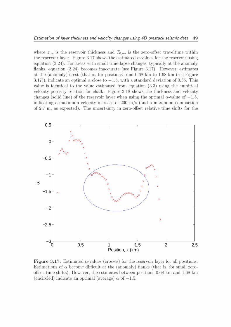
Estimation of layer thickness and velocity changes using 4D prestack seismic data 49
where zres is the reservoir thickness and T0,res is the zero-offset traveltime withinthe reservoir layer. Figure 3.17 shows the estimated α-values for the reservoir usingequation (3.24). For areas with small time-lapse changes, typically at the anomalyflanks, equation (3.24) becomes inaccurate (see Figure 3.17). However, estimatesat the (anomaly) crest (that is, for positions from 0.68 km to 1.68 km (see Figure3.17)), indicate an optimal α close to −1.5, with a standard deviation of 0.35. Thisvalue is identical to the value estimated from equation (3.3) using the empiricalvelocity-porosity relation for chalk. Figure 3.18 shows the thickness and velocitychanges (solid line) of the reservoir layer when using the optimal α-value of −1.5,indicating a maximum velocity increase of 200 m/s (and a maximum compactionof 2.7 m, as expected). The uncertainty in zero-offset relative time shifts for the
0 0.5 1 1.5 2 2.5−3
−2.5
−2
−1.5
−1
−0.5
0
0.5
Position, x (km)
α
Figure 3.17: Estimated α-values (crosses) for the reservoir layer for all positions.Estimations of α become difficult at the (anomaly) flanks (that is, for small zero-offset time shifts). However, the estimates between positions 0.68 km and 1.68 km(encircled) indicate an optimal (average) α of −1.5.

50 Field-data example
0 0.5 1 1.5 2 2.5−4
−3
−2
−1
0
1
Position, x (km)
∆ z
(m)
0 0.5 1 1.5 2 2.5
0
100
200
300
Position, x (km)
∆ v
(m/s
)
Figure 3.18: Estimated changes (solid line) in thickness (top) and velocity (bot-tom) for the reservoir layer (as a function of position) when using an optimal α-valueof −1.5. The dashed lines indicate the uncertainties.
reservoir layer is estimated to be 15 × 10−3 by assuming a deviation in zero-offsetrelative time shifts for both top and base reservoir of 0.3 × 10⁻³. This gives anuncertainty (marked as dashed lines in Figure 3.18) in the maximum estimatedreservoir velocity change (+200 m/s) of 85 m/s, when assuming an uncertainty of0.35 in the estimated α (of −1.5) for the reservoir.
We estimated an average α from the sea surface to the top reservoir horizon of−2.1. If we know the sea bed subsidence, this α-value can be used to estimatethe α-value for overburden rocks only, using equation (3.24). Bathymetry surveys(Hall et al., 2005) show a maximum sea bed subsidence of approximately 0.5 m inour area, corresponding to a maximum stretch of the overburden rocks of 2.2 m.This gives an α-value of −2.6 for the overburden rocks, which is very close to the

Estimation of layer thickness and velocity changes using 4D prestack seismic data 51
rock physics estimate based on equation (3.3) and Han’s (1986) empirical relationfor clay, which is −2.7. Tosaya and Nur’s (1982) relation for clay give a slightlydifferent value (−3.6).
3.5.3 Anisotropy
In cases with overburden thickness and velocity changes, we might expect changesin anisotropy. For simplicity we have chosen not to incorporate anisotropy in the de-veloped method. Investigations show that static anisotropy has almost no effect onthe method (equation (3.9)). However, large time-lapse anisotropy changes must beincluded. We test the method on a synthetic model that consists of one overburdenlayer with thickness 2500 m and velocity 2100 m/s, and a second layer which simu-lates a reservoir. The overburden layer has initially anisotropic parameters similarto Valhall; that is, Thomsen’s (1986) anisotropic parameters δ = 0.05 and ε = 0.05(see Le Rousseau and De Hoop, 2001; Guerrero et al., 2002). For the monitor case,the overburden layer undergoes a stretch of 2.0 m, and a vertical velocity decrease of4.5 m/s. Corresponding changes in the anisotropic parameters δ and ε are tested fortwo cases; that is, 1) 0.5% change in both ε and δ and 2) 1.0% change in both ε and δ.
The choices of change in anisotropic parameters (for the two given cases) are basedon Yongyi (2004). He links the anisotropic parameter ε to vertical (P-wave) veloci-ties and clay volume (based on laboratory measurements) as follows:
ε =0.7Vclay(vp − vp,water)
vp,quartz − vp,water − 2.29Vclay, (3.25)
where vp denotes the vertical velocity and Vclay denotes the clay volume. The pa-rameters vp,quartz = 6050 m/s and vp,water = 1500 m/s are velocities for quartz andwater, respectively. Assuming an average clay volume of 50% for the overburdenlayer gives ε ≈ 0.06 from equation (3.25), when using the initial vertical velocity of2100 m/s. Substituting the vertical velocity for the monitor case (that is, 2095.5m/s) in equation (3.25) gives a change in ε of 0.75% (when assuming constant clayvolume). For simplicity, we assume that δ and ε have changes of the same order;that is, around 0.75%.
For the overburden layer, we found the optimal α to be −2.1 for case 1 (that is, when∆ε/ε = ∆δ/δ = 0.5%) and −1.5 for case 2 (that is, when ∆ε/ε = ∆δ/δ = 1.0%).The modeled α = −2.6, which equals a deviation in the estimated α of 19% for case1 and 42% for case 2. The estimated values of α give ∆z = 2.5 m and ∆v = −4.4m/s for case 1 and ∆z = 3.1 m and ∆v = −3.9 m/s for case 2. The modeled valuesare ∆z = 2.0 m and ∆v = −4.5 m/s, which equals a deviation in the estimated ∆zand ∆v of 25% and 2% (respectively) for case 1, and 55% and 13% (respectively)for case 2. This shows that the uncertainty in estimated thickness and velocity

52 Discussion
changes becomes severe when the changes in anisotropic parameters exceed 1%.
3.6 Discussion
Static anisotropy is found to be much less of a problem than time-lapse changes inanisotropy. We find that changes of only 1% in the anisotropic parameters need tobe taken into account.
For the estimated α of −1.5 for the reservoir layer (field data), we assume thatthe base of the reservoir is constant in depth during reservoir compaction. Thisis not the case for a layer that consists of the same type of material as the sur-roundings, in which case the base of the layer tends to move upward during layercompaction (see Tura et al., 2005). At Valhall, hard chalk underlies the reservoirchalk, and we believe that this hard chalk is less affected by reservoir changes.However, a sequence of 0.4 km right below the reservoir layer shows time shifts(maximum 1-2 ms) that indicate stretch. An uplift of the base reservoir horizon atValhall is also predicted by Hatchell and Bourne (2005b). This means (equation(3.8)) that the magnitude of the estimated α is overestimated, and correspondinglythe velocity increase is also overestimated.
Our estimates of the dilation factor (α) is in good agreement with empirical rockphysics relations. However, it should be noted that these empirical relations arebased on ultrasonic measurements relating velocity to porosity. We do not knowto what extent such empirical relationships can be used for a dynamic case, wherevelocity changes are introduced by for instance stretching of the rock.
The proposed method can be further improved by utilizing data with larger offsets.In addition, new rock physics models can be used to constrain the α-parameterestimation. Geomechanical modeling and reservoir simulation can give additionalinformation (Hatchell et al., 2005; Vidal et al., 2002). Improved results can alsobe achieved by including ray-bending and by accounting for vertical variations in(relative) velocity changes.
The proposed method was tested on a sequence from the sea surface to the topreservoir horizon, and then, indirectly, the thickness and velocity changes for thereservoir layer and overburden rocks (for the Valhall Field) were estimated. It mayalso be possible to apply the method directly on one single layer (for example, thereservoir layer). However, investigations show that picked offset-dependent relativetime shifts become more uncertain when based on picks from both top and base

Estimation of layer thickness and velocity changes using 4D prestack seismic data 53
horizons of a layer, rather than a sequence from the sea surface to one (base) horizononly. In addition, correction terms are needed if the top of the layer is changing indepth, since our method was derived assuming that the top of the layer is constant(zero) in depth.
The proposed method is almost unaffected by velocity-depth ambiguities and er-rors in stacking velocity (see Bickel, 1990; Bube et al., 2004) which are well-knownphenomena in seismic exploration. This is due to the fact that we utilize offset-dependent time shifts (rather than time-lapse changes in stacking velocity). How-ever, it should be noted that stacking velocity is used to estimate the thickness (z),which is needed in equation (3.9). Nevertheless, investigations (of the overburdenestimated α = −2.1) show that the deviation in α is almost unaffected by uncer-tainties in z as large as 20%.
In all time-lapse monitoring, repeatability is crucial. Different sources and sourcedepths were used in the time-lapse surveys (1992-2002) from Valhall. This mightintroduce nonrepeatability (Landrø, 1999b) even though a good match is found.Further examples of nonrepeatability problems in time-lapse seismic are differencesin the source-receiver positions, changes in the water temperature, tidal differences,random noise in the recording units, and coherent noise such as free surface multi-ples. In addition, for cases with reservoir compaction and corresponding overburdenchanges, the elastic wavefield parameters and, further, the quality factor Q (damp-ing), change. Stewart et al. (1984) derived an equation that estimates the delayin traveltimes based on traveltimes, frequency ratios, and quality factor Q. Thequality factor Q can be estimated from a constant-Q model (Kjartansson, 1979).Combining the two models, assuming a constant Q equal to 70 for the baseline and75 for the monitor, gives a difference in traveltime delay of 0.1 ms between baselineand monitor. Another example, using Q equal to 70 and 90 for the baseline andmonitor, respectively, gives a time-lapse difference in traveltime delay of 0.5 ms.
3.7 Conclusions
Prestack analysis of time-lapse seismic traveltime shifts gives an opportunity todiscriminate between layer thickness and velocity changes, for both the reservoirlayer and the overburden layers. We find that the introduction of the dilation fac-tor (ratio between relative velocity changes and relative thickness changes) is bothpractical and a useful concept for the prestack time lapse analysis. The developedmethod links the relative change in traveltime (for a given offset) with the dilationfactor and the relative change in zero-offset traveltime, where lateral variations inrelative velocity changes are incorporated. Basic assumptions in the derivation ofthe equations are the assumption of one single horizontal layer, straight raypaths

54 Acknowledgments
and neglecting vertical changes in the velocity field. If the method is applied toa multilayer case we find that the errors increase if the velocity changes betweenthe layers are significant. For a synthetic model consisting of 5 overburden layersthat are stretched and a compacting reservoir layer, we find that our method can beapplied successfully to estimate the average dilation factor for the overburden layers.
For the top reservoir horizon at the Valhall Field we estimate a maximum sub-sidence of 2.7 m ± 1.6 m and a corresponding velocity decrease for the sequencefrom the sea surface to the top reservoir of 4.5 m/s ± 1.3 m/s. For the reservoirsection a maximum velocity increase of 200 m/s ± 85 m/s is calculated when relatedto the maximum top reservoir subsidence (of 2.7 m).
The method does not require any information or model for the mechanism cre-ating the velocity change. Discrimination between pressure, fluid, or compactionchanges should be performed in a preceding analysis step. Compared to measuredcompaction rates in other areas of this field, the estimated values are reasonable.
3.8 Acknowledgments
Thomas Røste acknowledges TOTAL for financial support, and Jerome Guilbot,Yahui Yin, and Ruben Sanchez for valuable discussions. We thank the Valhallpartnership (BP Norge AS, Amerada Hess Norge AS, A/S Norske Shell, and TotalE&P Norge AS) for providing data from the Valhall Field and permission to publishthis work, as well as Ole Jøran Askim, Olav Barkved, and Tron G. Kristiansen forsupport and discussions. We also acknowledge constructive comments from severalreviewers and Yonghe Sun for discussions in finalizing this paper. Martin Landrøand Alexey Stovas acknowledge the Norwegian Research Council for financial sup-port to the ROSE project at NTNU. Finally, we thank Øyvind Kvam for advice onmaking the synthetic model. The results and opinions presented in this paper donot necessarily reflect the view of the Valhall partnership.

Estimation of layer thickness and velocity changes using 4D prestack seismic data 55
3.A Rock physics
Well log observations show empirical relationships between velocity (v) and porosity(φ)given as (Han, 1986; Rafavich et al., 1984)
v = a − bφ, (3.A-1)
where a and b are positive constants. Differentiation of equation (3.A-1) and sub-stitution of b gives
dv
v=(1 − a
v
) dφ
φ. (3.A-2)
The uniaxial strain relationship reads (Guilbot and Smith, 2002)
dφ
1 − φ=
dz
z + dz, (3.A-3)
where z and dz denote thickness and thickness changes, respectively. By assum-ing small changes and substituting for φ (given by rearranging equation (3.A-1)),equation (3.A-3) reads
dφ
φ=
dz
z
(b
a − v− 1
). (3.A-4)
Substituting equation (3.A-4) into equation (3.A-2) gives
dv
v=
(a − b
v− 1
)dz
z. (3.A-5)
Equation (3.A-5) shows that relative thickness and velocity changes are linked bythe factor:
α =a − b
v− 1, (3.A-6)
which is spatially dependent since a, b, and v are expected to vary spatially.

56 Detailed derivation of the method
3.B Detailed derivation of the method
Assuming a one-layer model with straight raypaths, seismic two-way traveltime fora ray with CDP-position x0 and offset 2h can be expressed as
T (x0, h) =
√1 +
z2(x0)
h2
x0+h∫x0−h
dx
v(x). (3.B-1)
For the post-production (or monitor) case, the two-way traveltime is
T′(x0, h) =
√1 +
z2(x0)
h2
(1 +
∆z(x0)
z(x0)
)2x0+h∫
x0−h
dx
v(x)(1 + ∆v(x)
v(x)
) , (3.B-2)
where ∆v(x)/v(x) is assumed to vary with lateral position x, but not with depth.The square root and functions (1 + ∆z(x0)/z(x0))
2 and (1 + ∆v(x)/v(x))−1 inequation (3.B-2) can be expanded in Taylor series. Assuming small relative changesin velocity and thickness; that is, keeping only the first expanded term, equation(3.B-2) becomes
T′(x0, h) ≈
√1 +
z2(x0)
h2
(1 + 2
∆z(x0)
z(x0)
) x0+h∫x0−h
dx
v(x)
(1 − ∆v(x)
v(x)
)
T′(x0, h) =
√1 +
z2(x0)
h2+ 2
z2(x0)
h2
∆z(x0)
z(x0)
x0+h∫x0−h
dx
v(x)
(1 − ∆v(x)
v(x)
)
T′(x0, h) =
√1 +
z2(x0)
h2
√√√√1 +2z2(x0)
h2∆z(x0)z(x0)
1 + z2(x0)h2
x0+h∫x0−h
dx
v(x)
(1 − ∆v(x)
v(x)
)
T′(x0, h) ≈
√1 +
z2(x0)
h2
⎛⎝1 +
z2(x0)h2
∆z(x0)z(x0)
1 + z2(x0)h2
⎞⎠ x0+h∫
x0−h
dx
v(x)
(1 − ∆v(x)
v(x)
)
T′(x0, h) =
√1 +
z2(x0)
h2
(1 +
z2(x0)
h2 + z2(x0)
∆z(x0)
z(x0)
)
×x0+h∫
x0−h
dx
v(x)
(1 − ∆v(x)
v(x)
). (3.B-3)

Estimation of layer thickness and velocity changes using 4D prestack seismic data 57
From equations (3.B-1) and (3.B-3) the relative change in two-way traveltime be-comes
∆T (x0, h)
T (x0, h)=
(1 + z2(x0)
h2+z2(x0)∆z(x0)z(x0)
) x0+h∫x0−h
dxv(x)
(1 − ∆v(x)
v(x)
)x0+h∫x0−h
dxv(x)
− 1. (3.B-4)
By assuming small lateral variations in initial layer velocity in the vicinity of eachposition x0; that is, v(x) ≈ v(x0) for x0 − h ≤ x ≤ x0 + h, the term 1/v(x) can beput outside the integration signs (given in both the numerator and denominator ofequation (3.B-4)) and be cancelled out. Note, however, that the lateral variationsin ∆v are included; that is, ∆v = ∆v(x):
∆T (x0, h)
T (x0, h)≈
(1 + z2(x0)
h2+z2(x0)∆z(x0)z(x0)
)1
v(x0)
x0+h∫x0−h
dx(1 − ∆v(x)
v(x)
)1
v(x0)
x0+h∫x0−h
dx
− 1
∆T (x0, h)
T (x0, h)=
(1 + z2(x0)
h2+z2(x0)∆z(x0)z(x0)
) x0+h∫x0−h
dx(1 − ∆v(x)
v(x)
)2h
− 1. (3.B-5)

58 Detailed derivation of the method
Rearranging equation (3.B-5) gives
∆T (x0, h)
T (x0, h)=
1
2h
x0+h∫x0−h
dx
(1 − ∆v(x)
v(x)
)
+z2(x0)
h2 + z2(x0)
∆z(x0)
z(x0)
1
2h
x0+h∫x0−h
dx
(1 − ∆v(x)
v(x)
)− 1
∆T (x0, h)
T (x0, h)= 1 − 1
2h
x0+h∫x0−h
dx∆v(x)
v(x)+
z2(x0)
h2 + z2(x0)
∆z(x0)
z(x0)
− z2(x0)
h2 + z2(x0)
∆z(x0)
z(x0)
1
2h
x0+h∫x0−h
dx∆v(x)
v(x)− 1
∆T (x0, h)
T (x0, h)= − 1
2h
x0+h∫x0−h
dx∆v(x)
v(x)+
z2(x0)
h2 + z2(x0)
∆z(x0)
z(x0)
− z2(x0)
h2 + z2(x0)
∆z(x0)
z(x0)
1
2h
x0+h∫x0−h
dx∆v(x)
v(x), (3.B-6)
where the last term in equation (3.B-6) can be neglected for small changes in relativevelocity and thickness changes. This gives
∆T (x0, h)
T (x0, h)≈ − 1
2h
x0+h∫x0−h
dx∆v(x)
v(x)+
z2(x0)
h2 + z2(x0)
∆z(x0)
z(x0). (3.B-7)
The relative changes in thickness and velocity can be related to the relative changein vertical traveltime as
∆z(x)
z(x)≈(
1
1 − α
)∆T0(x)
T0(x),
∆v(x)
v(x)≈(
α
1 − α
)∆T0(x)
T0(x), (3.B-8)
which gives equation (3.B-7) on the following form:
∆T (x0, h)
T (x0, h)≈ z2(x0)
z2(x0) + h2
(1
1 − α
)∆T0(x0)
T0(x0)− 1
2h
(α
1 − α
) x0+h∫x0−h
dx∆T0(x)
T0(x).
(3.B-9)Equation (3.B-9) shows that there exists a relationship between the parameter α,the relative change in traveltime for zero offset, and the relative change in traveltimefor a given half-offset h.

Estimation of layer thickness and velocity changes using 4D prestack seismic data 59
3.C Testing equation (3.9) for a two-layer model
In order to test the accuracy of using the straight-ray approximation used in equa-tion (3.9) and test how accurate it can be when applied to a stack of several layers,we consider a two layer model, with initial layer thicknesses z1 and z2, respectively.Let the incidence angle in the first layer be θ1 and the ray angle in the second layerbe θ2. Then the two-way traveltime for the pre-stretch situation is given as
T = 2
[z1
v1 cos θ1+
z2
v2 cos θ2
]. (3.C-1)
The half-offset is given as
h = z1 tan θ1 + z2 tan θ2. (3.C-2)
After stretching (monitor survey), the offset is conserved; that is,
h = (z1 + ∆z1) tan(θ1 + ∆θ1) + (z2 + ∆z2) tan(θ2 + ∆θ2), (3.C-3)
where ∆θ represents change in ray angle due to stretching. Combining equations(3.C-2) and (3.C-3) and assuming that the changes in ray angles are small due tothe stretching of the layers, lead to
∆z1 tan θ1 + ∆z2 tan θ2 = −z1∆θ1(1 + tan2 θ1) − z2∆θ2(1 + tan2 θ2). (3.C-4)
Now we apply Snell’s law for initial and monitor cases:
sin θ1
v1=
sin θ2
v2, (3.C-5)
sin(θ1 + ∆θ1)
(v1 + ∆v1)=
sin(θ2 + ∆θ2)
(v2 + ∆v2). (3.C-6)
Combining equations (3.C-5) and (3.C-6) and assuming small changes in ray anglesgives
∆θ1 = tan θ1
(∆v1
v1
− ∆v2
v2
)+ ∆θ2
v1 cos θ2
v2 cos θ1
. (3.C-7)
Inserting equation (3.C-7) into equation (3.C-4) gives an explicit expression for thechange in ray angle in layer 2:
∆θ2 = −z1 tan θ1
(∆v1
v1− ∆v2
v2
)(1 + tan2 θ1) + ∆z1 tan θ1 + ∆z2 tan θ2
z1v1 cos θ2
v2 cos θ1(1 + tan2 θ1) + z2(1 + tan2 θ2)
. (3.C-8)
The traveltime after stretching for the two-layer model is given as
T′= 2
[z1 + ∆z1
(v1 + ∆v1) cos(θ1 + ∆θ1)+
z2 + ∆z2
(v2 + ∆v2) cos(θ2 + ∆θ2)
]. (3.C-9)
From equations (3.C-1) and (3.C-9) the relative traveltime shift can be computed,and compared to the one-layer approximation given in equation (3.9). An exampleof such a comparison is shown in Figure 3.2.

60 Uncertainty estimates
3.D Uncertainty estimates
Errors due to the approximations made from equation (3.6) to equation (3.9) canbe investigated step by step. The approximations made from equation (3.6) toequation (3.7) are summarized by equation (3.D-1) (for small thickness changes)and equation (3.D-2) (for small velocity changes).√
1 +z2(x0)
h2
(1 +
∆z(x0)
z(x0)
)2
≈√
1 +z2(x0)
h2
(1 +
z2(x0)
h2 + z2(x0)
∆z(x0)
z(x0)
),(3.D-1)
x0+h∫x0−h
dx
v(x)(1 + ∆v(x)
v(x)
) ≈x0+h∫
x0−h
dx
v(x)
(1 − ∆v(x)
v(x)
). (3.D-2)
These approximation steps lead to negligible error for general cases. As an examplefor equation (3.D-1), assuming h = 0.5 km, z = 2.5 km, and ∆z = 2.5 m (that is,∆z/z = 0.001) gives the left hand side (LHS) of equation (3.D-1) equal to 5.1039225and the right hand side (RHS) equal to 5.1039224, which corresponds to 0.000002 %relative error. Using ∆z/z = 0.01 in equation (3.D-1) gives LHS = 5.1480579 andRHS = 5.1480485 corresponding to 0.0002 % relative error. A similar examplefor equation (3.D-2), assuming h = 0.5 km, v = 2.0 km/s, and ∆v = −5 m/s(that is, ∆v/v = −0.0025, where we for simplicity assume ∆v(x) and v(x) laterallyconstant) gives the LHS in equation (3.D-2) equal to 0.501253 and the RHS equalto 0.501250, which corresponds to 0.0006% relative error. Using ∆v/v = −0.01in equation (3.D-2) gives LHS = 0.505051 and RHS = 0.505000 corresponding to0.010 % relative error.
The approximations from equation (3.7) to equation (3.9) can be summarized inthree steps:
x0+h∫x0−h
dx
v(x)
∆v(x)
v(x)≈ 1
v(x0)
x0+h∫x0−h
dx∆v(x)
v(x), (3.D-3)
1
v(x0)
x0+h∫x0−h
dx∆v(x)
v(x)≈ 1
v(x0)
(α
1 − α
) x0+h∫x0−h
dx∆T0(x)
T0(x), (3.D-4)
z2(x0)
h2 + z2(x0)
∆z(x0)
z(x0)
1
2h
x0+h∫x0−h
dx∆v(x)
v(x)≈ 0, (3.D-5)
where the approximation step given by equation (3.D-4) is only a substitution ofthe relative velocity changes; that is, ∆v(x)/v(x) ≈ (α/(1 − α))∆T0(x)/T0(x). Theapproximation given in equation (3.D-3) is the critical step. As an example, we

Estimation of layer thickness and velocity changes using 4D prestack seismic data 61
assume linear lateral variations in the layer velocity and velocity changes, and thatposition x is defined from zero to h; that is,
v(x) = v(0) + Ax
h, (3.D-6)
∆v(x) = ∆v(0) + Bx
h. (3.D-7)
Inserting equations (3.D-6) and (3.D-7) into equation (3.D-3), we obtain (skippingthe symmetric part of the integral)
h∫0
dx(∆v(0) + B xh)
(v(0) + Axh)2
≈ 1
v(0)
h∫0
dx(∆v(0) + B xh)
(v(0) + Axh)
. (3.D-8)
The integral on the LHS of equation (3.D-8) is equal to
−Ah∆v(0) + Bhv(0)
A2(A + v(0))− −Ah∆v(0) + Bhv(0)
A2v(0)+
B
A2h ln(
A
v(0)+ 1). (3.D-9)
The RHS of equation (3.D-8) is equal to
h
v(0)
[B
A−(
Bv(0)
A2− ∆v(0)
A
)ln(
A
v(0)+ 1)
]. (3.D-10)
As an example, we assume ∆v(0) = 0 (note, however, that the lateral variations in∆v(x) are still included by parameter B). This gives the LHS of equation (3.D-8)on the following form:
h
v(0)
[Bv2(0)
A2(A + v(0))− Bv(0)
A2+
Bv(0)
A2ln(
A
v(0)+ 1)
], (3.D-11)
and the RHS of equation (3.D-8) on the following form:
h
v(0)
[B
A− Bv(0)
A2ln(
A
v(0)+ 1)
]. (3.D-12)
By assuming A = B = 0.01v(0), the LHS of equation (3.D-8) is equal to 0.0049341 hv(0)
(from equation (3.D-11)), and the RHS of equation (3.D-8) is equal to 0.0049669 hv(0)
(from equation (3.D-12)) corresponding to 0.66% relative error. Using A = B =0.1v(0) in equation (3.D-8) gives LHS = 0.0440109 h
v(0)and RHS = 0.0468982 h
v(0)
corresponding to 6.56 % relative error. This means that the approximation givenby equation (3.D-3) holds as long as the lateral variations in the layer velocity andvelocity changes are small (inside the offset range 2h).

62 Uncertainty estimates
The third approximation step from equation (3.7) to equation (3.9), given by equa-tion (3.D-5), leads normally to small errors. As an example, assuming h = 0.5 km,z = 2.5 km, ∆v/v = −0.0025 (laterally constant), and ∆z/z = 0.001 gives the LHSin equation (3.D-5) equal to −2.4× 10⁻⁶. Since RHS = 0, this approximation leadsto an error of −2.4 × 10⁻⁶ in ∆T/T , where ∆T/T ≈ 0.0035 (from the given ∆v/vand ∆z/z); that is, an error of 0.069% in ∆T/T .

Estimation of layer thickness and velocity changes using 4D prestack seismic data 63
3.E Synthetic model parameters
For the forward model of the reservoir layer we express the P- and S-wave velocitiesas a function of porosity (φres); that is,
vp,res = a − bφres , vs,res = a′ − b′φres, (3.E-1)
where
a = 5500 m/s , b = 7000 m/s , a′ = 2845 m/s , b′ = 3621 m/s. (3.E-2)
The above given parameters are based on well logs. Differentiation of equation(3.E-1) yields
∆vp,res = −b∆φres, (3.E-3)
∆vs,res = −b′∆φres, (3.E-4)
where ∆φres denotes porosity changes in the reservoir. The reservoir density isassumed to follow the relation:
ρres = φresρF + (1 − φres)ρS , (3.E-5)
where ρF and ρS denote fluid and solid densities of the reservoir, respectively. As-suming that the fluid density is constant during compaction gives
∆ρres = (ρF − ρS)∆φres =ρF − ρres
(1 − φres)∆φres, (3.E-6)
by substituting ρS (obtained from equation (3.E-5)).
The uniaxial strain condition reads (Guilbot and Smith, 2002)
∆φres = (1 − φres)∆zres
zres + ∆zres
, (3.E-7)
where zres and ∆zres denote the reservoir thickness and thickness changes, respec-tively. Substituting ∆φres from equation (3.E-7) into the equations (3.E-3), (3.E-4),and (3.E-6) gives the following changes in the reservoir parameters:
∆vp,res = −b(1 − φres)∆zres
zres + ∆zres, (3.E-8)
∆vs,res = −b′(1 − φres)∆zres
zres + ∆zres, (3.E-9)
∆ρres = −(ρres − ρF )∆zres
zres + ∆zres
. (3.E-10)

64 Synthetic model parameters
Associated with the reservoir compaction we define overburden changes (for theforward model). For the overburden, Zi denotes the depth (from the sea surface)down to the base interface of layer i and the change in this depth denotes ∆Zi
(where positive ∆Zi corresponds to subsidence). The subsidence of the sea bedinterface is set to
∆Z1 = 0.8 × ∆zres. (3.E-11)
We assume that the subsidence of the overburden interfaces increases linearly withdepth (down to the top reservoir interface); that is,
∆Zi = Fi × ∆zres, (3.E-12)
where Fi is a depth dependent factor given as (only valid for the overburden layersbelow the sea bed; that is, 1 ≤ i ≤ 5)
Fi = 7.634 × 10⁻⁵Zi + 0.7939, (3.E-13)
where Zi (the depth down to the base interface of layer i) is given in meters. Thethickness change of an overburden layer i, ∆zi = ∆Zi−∆Zi−1, is given by equations(3.E-12) and (3.E-13); that is,
∆zi = 7.634 × 10⁻⁵(Zi − Zi−1)∆zres. (3.E-14)
Assuming mass conservation and layer expansion only in the z-direction, the relationbetween changes in thickness (∆zi) and density (∆ρi) for an overburden layer i isgiven as
ρi + ∆ρi
ρi=
zi
zi + ∆zi, (3.E-15)
where zi and ρi denote the thickness and density of layer i, respectively. For smallthickness changes, equation (3.E-15) can be written
∆ρi
ρi= −∆zi
zi. (3.E-16)

Estimation of layer thickness and velocity changes using 4D prestack seismic data 65
3.F Uncertainty in estimated α
The standard deviation of a function S = S(a, b, c, ...), where a, b, c, ... are parame-ters assumed to be independent of each other, is given by (Landrø, 2002)
δS =
√(∂S
∂aδa
)2
+
(∂S
∂bδb
)2
+
(∂S
∂cδc
)2
+ ... , (3.F-1)
where δa denotes the standard deviation or uncertainty in parameter a, etc.
An expression for α is found by rearranging equation (3.9):
α =
z2(x0)z2(x0)+h2
∆T0(x0)T0(x0)
− ∆T (x0,h)T (x0,h)
12h
x0+h∫x0−h
dx∆T0(x)T0(x)
− ∆T (x0,h)T (x0,h)
. (3.F-2)
Using the notations
f1 =z2(x0)
z2(x0) + h2, (3.F-3)
f2 =1
2h
x0+h∫x0−h
dx∆T0(x)
T0(x), (3.F-4)
f3 =∆T0(x0)
T0(x0), (3.F-5)
f4 =∆T (x0, h)
T (x0, h), (3.F-6)
the standard deviation in α can be written as
δα =
√(∂α
∂f1δf1
)2
+
(∂α
∂f2δf2
)2
+
(∂α
∂f3δf3
)2
+
(∂α
∂f4δf4
)2
, (3.F-7)
where
∂α
∂f1
=f3
f2 − f4
, (3.F-8)
∂α
∂f2=
f4 − f1f3
(f2 − f4)2, (3.F-9)
∂α
∂f3=
f1
f2 − f4, (3.F-10)
∂α
∂f4
=f1f3 − f2
(f2 − f4)2. (3.F-11)

66 Uncertainty in estimated α
Normal values for f1 are between 0.5 and 1.0, while f2, f3, and f4 are normally of theorder 10−3. All equations (3.F-8) to (3.F-11) are highly dependent of the differencebetween f2 and f4 which is normally of the order 10−3 to 10−4. Investigations showthat it is crucial to have differences between f2 and f4 larger than 1.0 × 10⁻⁴. Inaddition, any uncertainties in f1, f2, f3, and f4 must be small in order to estimateα accurately.
As an example, we investigate the uncertainty in an estimated α of −2.1 for asequence with thickness z = 2.5 km and half-offset h = 1.0 km. The uncertaintyin f1 is assumed to be 3.9% (which is obtained from equation (3.F-1) by assumingan uncertainty in both z and h of 10%). The difference between f2 and f4 is set to0.66×10−3. The standard deviation in zero-offset relative time shifts is estimated tobe 0.33×10⁻³ for the positions 0.80 km to 1.13 km (see Figure 3.12). The standarddeviation in far offset relative time shifts is estimated to 0.32 × 10⁻³ for position0.93 km (see Figure 3.13), when excluding the bad picked time shifts. Assumingan uncertainty of 0.3 × 10⁻³ for both zero-offset and offset-dependent relative timeshifts gives an uncertainty of 1.7 in the estimated α (of −2.1).

Chapter 4
Monitoring overburden layerchanges and fault movements fromtime-lapse seismic data on theValhall Field
Thomas Røste*, Martin Landrø*, and Paul Hatchell‡
*Norwegian University of Science and Technology,Department of Petroleum Engineering and Applied Geophysics,S.P.Andersens vei 15A, N-7491 Trondheim, Norway .‡Shell International Exploration and Production, Rijswijk, The Netherlands.
Accepted for publication in Geophysical Journal International in January 2007.Presented at the ROSE meeting in Trondheim, Norway, April 2006. Expanded ab-stract submitted to the 69th EAGE Conference & Exhibition, London, England,June 2007.
4.1 Abstract
A method developed by Røste et al. (2005), which discriminates between layer thick-ness and velocity changes, is tested on prestack time-lapse seismic ocean bottomcable (OBC) data from the Valhall Field. A key parameter in this discriminationprocess is the dilation factor, α, which is the relative velocity change divided bythe relative thickness change within a given layer. The high quality and good re-peatability of the OBC data enables us to estimate α with a reasonable accuracy
67

68 Introduction
for α-values between 0 and −5. For α-values below −5, complementary informa-tion, like for instance geomechanics is required. For the top reservoir horizon weestimate a maximum subsidence of 0.50 m ± 0.29 m and a corresponding velocitydecrease for the sequence from the sea bed to the top reservoir of 2.0 m/s ± 0.40 m/s.
Time-lapse distortion patterns with characteristic time shift versus offset signa-tures are observed. The positions and vertical extents of the distortion zones aredetermined from raypath considerations and modeling. The distortion zones cor-relate with buried faults, indicating that a (time-lapse) distortion zone might beproduced by a localized slip in a fault zone. We present an extended method whichallows for vertical (in addition to lateral) variations in the relative thickness andvelocity changes. This method can be viewed as a simplified version of time-lapsetomography, but involving less number of unknown parameters, giving more stabil-ity to the estimated changes in thickness and velocity. Using this technique, we areable to estimate α for positions with localized time-lapse distortions.
4.2 Introduction
Production-induced compaction is a significant drive mechanism for production inseveral North Sea reservoirs, especially the chalk reservoirs in the south. Guilbotand Smith (2002) utilized time isochron differences from 4D seismic data to detectcompaction and subsidence at the Ekofisk Field. They observed seismic time shiftsup to 12-16 ms between 1989 and 1999, related to compaction values of up to 6 mfor the reservoir chalk formation. Røste et al. (2005) developed a method, basedon prestack time-lapse seismic data, which discriminates between changes in layerthickness and velocity. They estimated a subsidence up to 2.7 m for the top reser-voir horizon at the Valhall Field (in the southern part of the field) from 1992 to2002. Reservoir compaction might have implications for production by changingpermeabilities and, hence, the production performance (Hall et al., 2005). In ad-dition, compaction might lead to subsidence of the sea bed. At the Valhall Field,Barkved and Kristiansen (2005) report a maximum subsidence of the sea bed largerthan 5.4 m (since the field came on production in 1982) and increasing at 0.25 m peryear. It is typical for these fields that the sea bed subsidence is less than the cor-responding reservoir compaction, meaning that the overburden rocks are stretched.Often the change in geomechanical stress state for the overburden rocks leads todamage in existing wells (especially when significant shear stresses are introducedas a byproduct of the reservoir compaction). It is therefore of importance to mapthe velocity and thickness changes during production not only for the reservoir it-self, but also for the overburden rocks. Between the wells, time-lapse seismic datais a complementary tool for obtaining this information, and the combined use ofrepeated seismic measurements and geomechanical knowledge is expected to be im-

Monitoring overburden layer changes and fault movements from time-lapse seismicdata on the Valhall Field 69
portant in future monitoring projects.
Several authors (Ewing, 1985; White and Morton, 1997; Morton et al., 2006) showthat there is a coupling between reservoir compaction and slip along growth faultsthat become active when sufficiently large volumes of fluid (oil, gas, or formationwater) are produced. Fluid extraction may cause pore pressure decrease withinthe rocks and alter the state of stress near the faults (Geertsma, 1973). At theValhall and Ekofisk fields, Zoback and Zinke (2002) demonstrate that as a resultof production-induced pore pressure and stress changes, normal faulting appearsto have spread out from the crests of the structures on to the flanks. Reynoldset al. (2003) determined the relative attendant risk of reactivation of faults in theBight Basin by evaluating the in situ stress field. Mildren et al. (2002) tried topredict reactivation of faults by using the FAST (Fault Analysis Seal Technology)technique. Monitoring fault movements is important for several reasons. Most im-portant, hazards are associated with wells crossing reactivated faults (Alsos et al.,2002). Maury et al. (1992) discuss how slipping faults can pose serious problemssince it may cause casing failure. Kristiansen (2004) reviews the drilling history atValhall with main focus on the increasing problems in the late 90’s where severalvery expensive wells were lost. He concludes that wells (particularly high anglewells) are vulnerable for changes in stress changes and cavings from fault zones(see also Kristiansen, 1998). Barkved et al. (2003) report a strong correlationbetween overburden faults and drilling problems at the Valhall Field. Casing de-formations are expected to be part of the operational cost at Valhall (Kristiansenet al., 2000). In the reservoir zone, reactivation of faults might lead to leakage ofhydrocarbons and affect the reservoir drainage patterns. Fault seal breach in theNorth Sea (Gaarenstroom et al., 1993), the Penola Through (Jones et al., 2000),and the Gulf of Mexico (Finkbeiner et al., 2001) has been related to faulting andfracturing associated with the in situ stress. A fault can be a transmitter of orbarrier to fluid and pressure communication. Cerveny et al. (2004) discuss severalfault-seal analysis methods which evaluate the flow potential across a fault. Reviland Cathles (2002) show an example from the Gulf of Mexico where fluids migrateinto active growing faults. Based on seismic data and wellbore information, Allan(1989) diagrams are often used to identify potential petroleum leak points along afault strike. Reactivated faults can also have close relationship with earthquakes.Zoback and Zinke (2002) recorded numerous microearthquakes at the Valhall Fieldduring a six week monitoring period. They found the microearthquakes consistentwith a normal faulting stress regime. Chen and Bai (2006) built a model whichrelates the growth of microcracks with the occurrence of earthquakes.
The Valhall Field, situated in the southern part of the Norwegian North Sea, isa high-porosity Late Cretaceous chalk (porosities between 35-50%). The daily pro-duction is on the order of 100 000 barrels of light oil. The expected recovery rate

70 Introduction
in 1982 was 14%, a figure which has now increased to 40%. Time-lapse seismicmonitoring with high quality in addition to improved methods to interpret and uti-lize the seismic might increase the recovery further. In 2003, a permanent oceanbottom cable (OBC) array was installed at the Valhall Field, initiating the ”Lifeof Field Seismic” (LoFS) program which includes a series of 3D OBC surveys. Thefirst survey was acquired from September to November 2003 with subsequent sur-veys acquired in intervals of approximately 4 months. Results from the earliestsurveys confirm that the system can provide high quality data with good repeata-bility (Kommedal et al., 2004; Barkved, 2004).
In the present paper we investigate time-lapse changes on 2D prestack time-lapseseismic OBC lines from the LoFS survey 1 and survey 3. The 2D lines are situatedin the south-east part of the Valhall Field. By utilizing a method developed byRøste et al. (2005), changes in thickness and velocity are estimated for a sequencefrom the sea bed to the top reservoir horizon for one of the 2D lines. This methodutilizes time-lapse traveltime shifts for all offsets to find the dilation factor α whichdiscriminates between layer thickness changes and velocity changes. An advantageof this method is that no information or model is required for the mechanism cre-ating the velocity and thickness changes.
The LoFS data shows time shift patterns (between surveys 1 and 3) that movesystematically with offset. Analogous signatures have earlier been observed for sin-gle prestack surveys (e.g. Allen and Bruso, 1989; Fagin, 1996; Hatchell, 2000) andare associated with shallow distortion zones. As far as we know, such distortionsin time-lapse seismic are not so common. The location of the distortion zones aredetermined from geometry and raypath considerations. At least one of the distor-tions for the time-lapse time shifts observed between LoFS survey 1 and 3 is locatedin the vicinity of an existing fault. The distortions can be produced by a localizedslip in this observed fault zone creating changes in the rock properties framework.A time-lapse synthetic model is created to match the observed time shifts. To findthe dilation factor α for positions with time-lapse distortions we must account forvertical variations (in addition to lateral variations) in the relative velocity andthickness changes. An extended method is introduced to describe such positions.

Monitoring overburden layer changes and fault movements from time-lapse seismicdata on the Valhall Field 71
4.3 Discrimination between layer thickness and
velocity changes
It is important to notice that time-lapse seismic time shifts capture the combinedeffects of velocity and thickness changes within a given layer. The relative timeshift for zero offset can be expressed in terms of the relative thickness change andvelocity change as (Landrø and Stammeijer, 2004; Røste et al., 2005; Hatchell andBourne, 2005b)
∆T0(x0)
T0(x0)≈ ∆z(x0)
z(x0)− ∆v(x0)
v(x0), (4.1)
where T0 represents two-way traveltime for zero offset, z is the layer thickness, andv is the layer velocity. The parameter x0 denotes the global x-coordinate for agiven CDP-location (position), and ∆T0, ∆z, and ∆v represent changes in verticaltwo-way traveltime, thickness, and velocity, respectively. The basic assumption inequation (4.1) is that all relative changes are small; that is, ∆z
z<< 1 and ∆v
v<< 1.
As a first order approximation for a relation between relative thickness and velocitychanges for a given subsurface layer we assume that the two changes are proportionalto each other (Røste et al., 2005):
∆v(x0)
v(x0)≈ α
∆z(x0)
z(x0), (4.2)
where the dilation factor α < 0 is a parameter dependent on the rock properties ofthe layer. This is a crucial parameter, since it determines the ratio between veloc-ity and thickness changes. In general, α varies with spatial coordinates. However,similar to Røste et al. (2005, 2006), we assume that α is constant for the sequenceof layers we study.
The dilation factor α can be estimated based on time shift analysis. For a prestackCDP gather at position x0, the seismic two-way traveltime for a raypath with offset2h can be expressed as an integral over the total raypath length S,
T (x0, h) =
∫S
ds
v(s), (4.3)
where v(s) denotes the P-wave velocity at the ray position s(x0, h). Assume a one-layer model with a P-wave velocity field, v(x), that varies along the lateral positionx, but is nonvarying with depth. By assuming straight raypaths, it can be shownthat (similar to assuming average slowness within the offset range 2h)
T (x0, h) =
√1 +
z2(x0)
h2
x0+h∫x0−h
dx
v(x), (4.4)

72 Discrimination between layer thickness and velocity changes
where z(x0) represents the layer thickness at the CDP-position x0. Equation (4.4)describes the initial (or pre-production) case. For the post-production case, we findthat it is essential to include the lateral variations in velocity changes, since it isvery likely that such changes will occur both within the reservoir layer as well asthe overburden layers of a producing hydrocarbon reservoir (see also Røste et al.,2006). From equation (4.4), the two-way prestack traveltime for the monitor case(for a one-layer model) is then given as
T′(x0, h) =
√1 +
z2(x0)
h2
(1 +
∆z(x0)
z(x0)
)2x0+h∫
x0−h
dx
v(x)(1 + ∆v(x)
v(x)
) , (4.5)
where the relative change in velocity, ∆v(x)v(x)
, might vary laterally but not with depth.
(Note that variations in thickness changes only affect the multiplier outside the in-tegral in equation (4.5) when assuming straight raypaths.) Assuming small relativechanges in velocity and thickness, the relative change in two-way traveltime becomes(see Appendix 4.A)
∆T (x0, h)
T (x0, h)≈
(1 + z2(x0)
z2(x0)+h2∆z(x0)z(x0)
) x0+h∫x0−h
dxv(x)
(1 − ∆v(x)
v(x)
)x0+h∫x0−h
dxv(x)
− 1. (4.6)
From equations (4.1) and (4.2), the relative changes in layer thickness and velocitycan be related to the relative change in two-way vertical traveltime T0:
∆z(x0)
z(x0)≈(
1
1 − α
)∆T0(x0)
T0(x0),
∆v(x0)
v(x0)≈(
α
1 − α
)∆T0(x0)
T0(x0). (4.7)
By assuming small lateral variations in initial layer velocity in the vicinity of eachposition x0; that is, v(x) ≈ v(x0) for x0 − h ≤ x ≤ x0 + h, equation (4.6) canbe written in the simple form given by equation (4.8) (see Appendix 4.A). Note,however, that we include the lateral variations in ∆v; that is, ∆v = ∆v(x).
∆T (x0, h)
T (x0, h)≈ z2(x0)
z2(x0) + h2
(1
1 − α
)∆T0(x0)
T0(x0)− 1
2h
(α
1 − α
) x0+h∫x0−h
dx∆T0(x)
T0(x). (4.8)
The relative change in two-way traveltime (for a given half-offset h) is thereforedependent on α and the estimated relative change in vertical traveltime. (Notethat the integration sign in equation (4.8) in practice means summation, since timeshift estimations only exist for discrete positions (or CDPs).) The parameter αis determined by minimizing the least square error in relative traveltime change(equation (4.8)) over the entire offset range. This α-value is then inserted intoequation (4.7) to obtain the changes in layer thickness and velocity. Røste et al.,2006 discuss in detail the approximations made for equation (4.8).

Monitoring overburden layer changes and fault movements from time-lapse seismicdata on the Valhall Field 73
4.4 Estimate α from permanent OBC data
The method (given by equation (4.8)) is tested on a prestack time-lapse 2D OBCline situated in the south-east part of the Valhall Field (denoted l in Figure 4.1),acquired from survey 1 and survey 3 in the LoFS project. The selected 2D line
Amplitude difference map
Figure 4.1: Amplitude difference map of the top reservoir horizon in the southpart of the Valhall Field (between LoFS survey 1 and survey 3). The two selectedLoFS 2D lines (marked) follow buried cables. (The buried cables are given as dottedlines.)

74 Estimate α from permanent OBC data
follows a buried receiver cable, leading to excellent inline distribution of offsets.The data is corrected for tidal statics and a frequency-wavenumber filter was ap-plied to decrease multiple energy (Yilmaz, 1987). In addition, the signal to noiseratio and repeatability was increased by stacking 5 shots to each receiver, leadingto normalized root-mean-square (NRMS) of 0.41 for a 1.0 s time gate centered at2.0 s. Further, a 5x5 mixing operation of traces improved the NRMS to 0.19 for thesame time gate (of 1.0 s). This operation resulted in an effective offset spacing of200 m between the traces. The original offset spacing was 50 m. The total lengthof the selected 2D line is 2.3 km and, for simplicity, we define the north-west andsouth-east ends of this selection as positions x = 0 km and x = 2.3 km, respectively.Figure 4.2 shows the quality and repeatability of the LoFS data. Here the data fromLoFS survey 1 for zero offset is shown inside the letters ”NTNU” together with sur-vey 3 given in the background. The top of the reservoir is around 2.6 s (two-way
Figure 4.2: LoFS survey 1 (inside the letters ”NTNU”) shown together withsurvey 3 (in the background) for zero offset, as a function of position. Note thegood quality and high repeatability of the data.

Monitoring overburden layer changes and fault movements from time-lapse seismicdata on the Valhall Field 75
traveltime), corresponding to approximately 2.5 km in depth. We investigate anoverburden sequence from the sea bed to this top reservoir horizon.
The prestack events from the top reservoir horizon are picked for interpolated max-imum amplitudes. To increase the accuracy of the picked zero-offset traveltime(T0) (for a given position x0), it is normal to stack the picked offset-dependenttraveltimes (T ) by assuming standard hyperbolic moveout (Dix, 1955); that is,
T 2(x0, h) = T 20 (x0) +
4
V 2rms(x0)
h2, (4.9)
where h denotes half-offset and Vrms denotes rms velocity. Due to the high quality ofthe LoFS data, zero-offset traveltimes are estimated by stacking only the near offsets(that is, offsets below 1 km). Figure 4.3 shows the estimated (crosses) and laterallysmoothed (solid line) relative time shifts for zero offset for the top reservoir horizon.
0 0.5 1 1.5 2−1
−0.5
0
0.5
1
1.5
2
Position, x (km)
∆T0 /
T 0 (10
−3)
Figure 4.3: Estimated (crosses) and smoothed (solid line) relative zero-offset timeshifts for the top reservoir horizon.
76 Estimate α from permanent OBC data
The LoFS data shows high degree of repeatability, making it possible to detectsubtle traveltime changes. This is shown in Fig. 4.4, where LoFS data from survey1 (solid black line) is shown together with survey 3 (solid blue line) for position 1.6km at 1.0 km offset. For the reservoir section, solid black line is survey 1 and solidred line is survey 3 (top right). By interpolating the seismic we are able to detect atraveltime shift (measured at the maximum amplitude) of around 1.5 ms (bottomright). The repeatability is maintained for increasing offsets. Fig. 4.5 shows LoFSdata from survey 1 (solid black line) together with survey 3 (solid blue line) at 2.0km offset (for same position 1.6 km). For the reservoir section, solid black line issurvey 1 and solid red line is survey 3 (top right). A traveltime shift of 1.0 ms isdetected for interpolated maximum amplitude (bottom left).
Our analysis follows the method of Røste et al. (2005): For an initial guess ofα, equation (4.8) gives corresponding (relative) time shifts for different half-offsets(h) which can be compared with the picked time shifts. We search for the α-valuethat leads to minimum least square error between the estimated and picked relativetime shifts, for all offsets. Figure 4.6 shows this procedure (for the sequence fromthe sea bed to the top reservoir horizon) for the 4 positions x = 0.3 km, x = 0.35km, x = 0.4 km, and x = 0.45 km: Starting with an initial α-value of 0 in equation(4.8), we search in steps of −0.1 within the span from 0 to −5, until we obtain anoptimal α-value (solid line), for each position, that gives the best fit to the pickedrelative time shifts (crosses). (Multiple picked time shifts for a given offset occurdue to opposite shooting directions.) The dashed lines in Figure 4.6 correspond tothe initial and last guess of α; that is, α = 0 and α = −5. The positions shownin Figure 4.6 (especially position x = 0.35 km) indicate an optimal α-value around−5. For position x = 0.3 km, picked relative time shifts seem to be uncertain foroffsets around 0.5 km, which might explain why the optimal α is slightly above−5 for this position. The picked relative time shifts for positions x = 0.4 km andx = 0.45 km indicate an optimal α-value slightly below −5. This might be correct;however, it is difficult to discriminate optimal α-values below −5, and we thereforechoose to stop our search at α = −5.
The difficulty of distinguishing α for decreasing values is shown in Figure 4.7 forposition x = 0.35 km. Here α-values ranging from 0 to −20 are inserted in equation(4.8) to estimate relative time shifts as a function of offset. When the absolutemagnitude of α is large, changes in α of the order 1 have negligible influence onthe factors ( 1
1−α) and ( α
1−α) in equation (4.8), and, consequently, the relative time
shifts are almost unchanged. This is obtained in Figure 4.7 for α-values below −5.
Figure 4.6 shows the positions from the investigated 2D line that have the bestsensitivity in α; that is, various values of α (within the range 0 to −5) give clearlydistinct results from equation (4.8). Acceptable sensitivity in α is also observed for

Monitoring overburden layer changes and fault movements from time-lapse seismicdata on the Valhall Field 77
Figure 4.4: Left: LoFS data from survey 1 (solid black line) together with survey 3(solid blue line) at 1.0 km offset for position 1.6 km. For the reservoir section, blacksolid line is survey 1 and red solid is survey 3 (top right). Due to the high degreeof repeatability we are able to detect subtle traveltime changes. Interpolating theseismic and picking for maximum amplitude gives a time shift (measured at themaximum amplitude) of 1.5 ms (bottom left).
the 4 positions x = 2.15 km, x = 2.2 km, x = 2.25 km, and x = 2.3 km. Thesepositions are shown in Figure 4.8, where the optimal fitted α-values (solid lines) ofthe picked relative time shifts (crosses) again indicate an α-value close to −5. (Thedashed lines indicate the initial and last guess of α; that is, α = 0 and α = −5.)
For the chosen 2D line we found locations characterized by both low sensitivityin α as well as good sensitivity in α. Note that the sensitivity in α is not dependenton the noise-level. Low sensitivity in α seems to occur for positions with small timeshifts, especially observed for the positions from x = 0.9 km to x = 1.4 km. Figure4.9 shows 4 of these positions; that is, positions x = 1.05 km, x = 1.1 km, x = 1.15km, and x = 1.2 km. Here the small size of the window between the initial and last

78 Estimate α from permanent OBC data
Figure 4.5: Repeatability is maintained for higher offsets. At the left, LoFS datafrom survey 1 (solid black line) is shown together with survey 3 (solid blue line)at 2.0 km offset (for position 1.6 km). For the reservoir section, black solid lineis survey 1 and red solid is survey 3 (top right). A subtle time shift of 1.0 ms isdetected for interpolated maximum amplitude (bottom left).
guess of α (that is, α = 0 and α = −5) (dashed lines) makes it impossible to find atrustable α-value. However, such positions are easy to detect and can be excludedwhen determining the optimal α-value for all positions.
Results and uncertainties
The method, given by equation (4.8), is highly dependent on the accuracy of thepicked zero-offset and offset-dependent time shifts. Obviously, data quality hasa significant impact on our ability to estimate α from time-lapse prestack seismicdata. Values of α down to −5 can be determined; however, below this limit, the un-certainties are large (as underlined in Figure 4.7). The standard deviation (denoted

Monitoring overburden layer changes and fault movements from time-lapse seismicdata on the Valhall Field 79
0 0.5 1 1.5 2
0
0.5
1
1.5
2
Position, x = 0.3 km
Offset (km)
∆T/T
(10
−3)
α = 0
α = −5
0 0.5 1 1.5 2
0
0.5
1
1.5
2
Position, x = 0.35 km
Offset (km)
∆T/T
(10
−3)
α = 0
α = −5
0 0.5 1 1.5 2
0
0.5
1
1.5
2
Position, x = 0.4 km
Offset (km)
∆T/T
(10
−3)
α = 0
α = −5
0 0.5 1 1.5 2
−0.5
0
0.5
1
1.5
Position, x = 0.45 km
Offset (km)
∆T/T
(10
−3) α = 0
α = −5
Figure 4.6: Example of finding α (for the sequence from the sea bed to the topreservoir horizon) for the 4 positions x = 0.3 km, x = 0.35 km, x = 0.4 km, andx = 0.45 km. For each position, the solid line indicates the best fit of the pickedrelative time shifts (crosses) as a function of offset. The dashed lines correspondto the initial and last guess of α; that is, α = 0 and α = −5. These 4 positionsindicate an α around −5.
δ) in α can be given as (Røste et al., 2006)
δα =
√(∂α
∂f1δf1
)2
+
(∂α
∂f2δf2
)2
+
(∂α
∂f3δf3
)2
+
(∂α
∂f4δf4
)2
, (4.10)

80 Estimate α from permanent OBC data
0 0.5 1 1.5 2
0
0.5
1
1.5
2
Position, x = 0.35 km
α = 0
α = −1
α = −2 α = −3 α = −4 α = −5 α = −10 α = −20
Offset (km)
∆T/T
(10
−3)
Figure 4.7: Estimated relative time shifts (as a function of offset) for several valuesof α for position x = 0.35 km. The solid line indicates the optimal α = −5. Notethe increased difficulty of distinguishing α-values as α decreases. The red and greenvertical bars indicate the standard and mean deviations (respectively) in pickedrelative time shifts.
where
∂α
∂f1=
f3
f2 − f4, (4.11)
∂α
∂f2=
f4 − f1f3
(f2 − f4)2, (4.12)
∂α
∂f3=
f1
f2 − f4, (4.13)
∂α
∂f4=
f1f3 − f2
(f2 − f4)2, (4.14)

Monitoring overburden layer changes and fault movements from time-lapse seismicdata on the Valhall Field 81
0 0.5 1 1.5 2 2.5−1
−0.5
0
0.5
1Position, x = 2.15 km
Offset (km)
∆T/T
(10
−3)
α = 0
α = −5
0 0.5 1 1.5 2 2.5−1
−0.5
0
0.5
1Position, x = 2.2 km
Offset (km)
∆T/T
(10
−3)
α = 0
α = −5
0 1 2 3−1
−0.5
0
0.5
1Position, x = 2.25 km
Offset (km)
∆T/T
(10
−3)
α = 0
α = −5
0 1 2 3−1
−0.5
0
0.5
1Position, x = 2.3 km
Offset (km)
∆T/T
(10
−3)
α = 0
α = −5
Figure 4.8: Example of finding α (for the sequence from the sea bed to the topreservoir horizon) for the 4 positions x = 2.15 km, x = 2.2 km, x = 2.25 km, andx = 2.3 km. For each position, the solid line indicates the best fit of the pickedrelative time shifts (crosses) as a function of offset. The dashed lines correspond tothe initial and last guess of α; that is, α = 0 and α = −5. Similar to Figure 4.6,the above positions indicate an α close to −5.
and
f1 =z2(x0)
z2(x0) + h2, (4.15)
f2 =1
2h
x0+h∫x0−h
dx∆T0(x)
T0(x), (4.16)
f3 =∆T0(x0)
T0(x0), (4.17)
f4 =∆T (x0, h)
T (x0, h). (4.18)

82 Estimate α from permanent OBC data
0 0.5 1 1.5 2−1
−0.5
0
0.5
1Position, x = 1.05 km
Offset (km)
∆T/T
(10
−3)
α = 0
α = −5
0 0.5 1 1.5 2−1
−0.5
0
0.5
1Position, x = 1.1 km
Offset (km)
∆T/T
(10
−3)
α = 0
α = −5
0 0.5 1 1.5 2−1
−0.5
0
0.5
1Position, x = 1.15 km
Offset (km)
∆T/T
(10
−3) α = 0
α = −5
0 0.5 1 1.5 2−1
−0.5
0
0.5
1Position, x = 1.2 km
Offset (km)
∆T/T
(10
−3) α = 0
α = −5
Figure 4.9: Example of 4 positions (x = 1.05 km, x = 1.1 km, x = 1.15 km, andx = 1.2 km) with low sensitivity in α. The small size of the window between theinitial and last guess of α (that is, α = 0 and α = −5) (dashed lines) makes itimpossible to find a trustable α-value.
Relative time shifts (also denoted f4) can be related to α according to equation(4.8); that is,
∆T (x0, h)
T (x0, h)≈ z2(x0)
z2(x0) + h2
(1
1 − α
)∆T0(x0)
T0(x0)− 1
2h
(α
1 − α
) x0+h∫x0−h
dx∆T0(x)
T0(x). (4.19)
Equations (4.10) to (4.19) make it possible to find the standard deviation in α ver-sus two key parameters: α itself and the uncertainty in the picked time shifts. Anexample is shown in Figure 4.10 for a picked time shift with offset 1.0 km (thatis, h = 0.5 km). Here a layer with initial thickness z = 2.5 km undergoes changescorresponding to relative zero-offset time shifts (∆T0
T0) (laterally constant) equal to
2.0 · 10−3. The uncertainty in z2
z2+h2 (denoted δf1 in equation (4.10)) is assumed
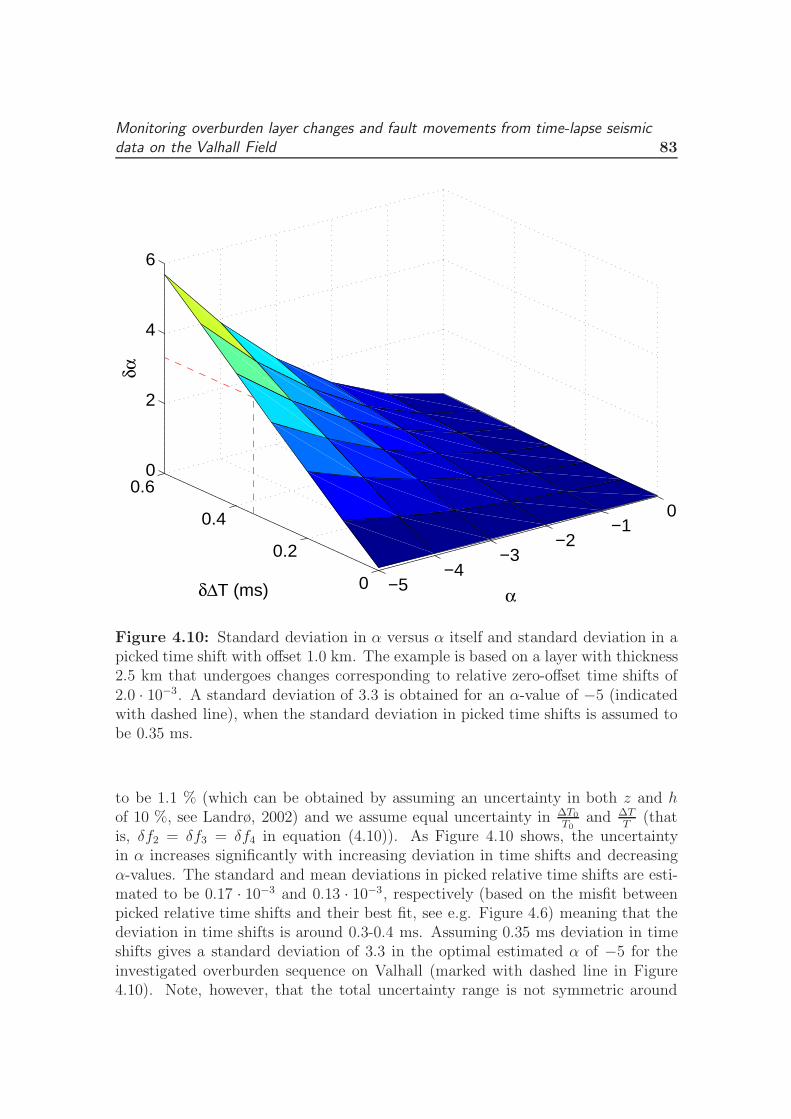
Monitoring overburden layer changes and fault movements from time-lapse seismicdata on the Valhall Field 83
−5−4
−3−2
−10
0
0.2
0.4
0.60
2
4
6
αδ∆T (ms)
δα
Figure 4.10: Standard deviation in α versus α itself and standard deviation in apicked time shift with offset 1.0 km. The example is based on a layer with thickness2.5 km that undergoes changes corresponding to relative zero-offset time shifts of2.0 · 10−3. A standard deviation of 3.3 is obtained for an α-value of −5 (indicatedwith dashed line), when the standard deviation in picked time shifts is assumed tobe 0.35 ms.
to be 1.1 % (which can be obtained by assuming an uncertainty in both z and hof 10 %, see Landrø, 2002) and we assume equal uncertainty in ∆T0
T0and ∆T
T(that
is, δf2 = δf3 = δf4 in equation (4.10)). As Figure 4.10 shows, the uncertaintyin α increases significantly with increasing deviation in time shifts and decreasingα-values. The standard and mean deviations in picked relative time shifts are esti-mated to be 0.17 · 10−3 and 0.13 · 10−3, respectively (based on the misfit betweenpicked relative time shifts and their best fit, see e.g. Figure 4.6) meaning that thedeviation in time shifts is around 0.3-0.4 ms. Assuming 0.35 ms deviation in timeshifts gives a standard deviation of 3.3 in the optimal estimated α of −5 for theinvestigated overburden sequence on Valhall (marked with dashed line in Figure4.10). Note, however, that the total uncertainty range is not symmetric around

84 Estimate α from permanent OBC data
the optimal α-value of −5, since the distribution of α is non-linear (Figure 4.7).The standard deviation in picked relative time shifts of 0.17 · 10−3 indicates thatα lies within the range −3 < α < −25 (marked as vertical red bar in Figure 4.7),while the mean deviation in relative time shifts (of 0.13 · 10−3) indicates a narrowerrange for α; that is, −3.4 < α < −17 (marked as vertical green bar in Figure 4.7).Both results show that we are able to exclude α-values between 0 and −3 for theinvestigated overburden rocks.
Figure 4.11 shows the estimated changes in thickness and velocity (solid line) forthe investigated sequence when using the optimal α-value of −5, together with un-certainties (dashed lines) correlated to an uncertainty of 3.3 in the optimal α (of−5). The solid dots indicate the initial guess of α; that is, α = 0. The estimated
0 0.5 1 1.5 2
−2
0
2α = 0
α = −5
Position, x (km)
∆z (m
)
0 0.5 1 1.5 2
−2
0
2
α = 0
α = −5
Position, x (km)
∆v (m
/s)
Figure 4.11: Estimated changes (solid line) in thickness (top) and velocity (bot-tom), together with indicated uncertainties (dashed lines) as a function of position(for the sequence from the sea bed to the top reservoir horizon) when using theoptimal α-value of −5. The solid dots correspond to the initial guess of α; that is,α = 0.

Monitoring overburden layer changes and fault movements from time-lapse seismicdata on the Valhall Field 85
optimal result in Figure 4.11 indicates a maximum subsidence of the top reservoirhorizon of 0.50 m (with deviation 0.29 m) and a maximum velocity decrease for theoverburden sequence of 2.0 m/s (with deviation 0.40 m/s).
4.5 Time-lapse distortions
In the second 2D line shown in Figure 4.1 (denoted l′) we observe time shift patternsthat move systematically with offset. The positions on line l′ are denoted x′ andrange from x′ = 0 km (north-west) to x′ = 2.3 km (south-east). Figure 4.12 showsthe picked relative time shifts (crosses) for the top reservoir horizon as a functionof offset for the positions x′ = 1.55 km to x′ = 1.8 km. Note the marked positivetime shifts around zero offset for position x′ = 1.55 km (shown by arrow in Figure4.12a). These time shifts move systematically with offset as the position increases(Figure 4.12b-4.12f), as shown by the arrow. In top of Figure 4.13, the same pickedtime shifts are displayed in the offset versus position domain (where the positiveand negative offsets only indicate opposite shooting directions). Here the time shiftpattern from the previous figure is clearly visible as a diagonal feature, moving fromzero offset at position x′ = 1.55 km towards increasing offset distance as the positionincreases. In addition, a similar feature, starting at position x′ = 0.4 km for zerooffset, is observed with marked negative time shifts. Both features are indicatedwith solid lines in top of Figure 4.13.
Similar patterns as shown in Figure 4.13 (top) have been previously observed on 3Dprestack datasets and are attributable to shallow velocity distortion zones. Hatchell(2000) observed transmission distortions that produce anomalous amplitude versusoffset (AVO) signatures on 3D seismic data at two locations in the Gulf of Mexico.He explains the distortion zones by velocity changes across faults and unconformitysurfaces. Fagin (1996) presents an example of seismic distortions (that is, time sagsand time pull-ups) resulting from extensional faults in the Wilcox trend of southTexas. His analysis shows that these distortions are produced by faults related tothe stratigraphic-velocity alternations in the Wilcox Formation. Time anomaliesattributable to growth faults are also discussed by Allen and Bruso (1989). Furtherdiscussions on transmission distortions are given by Kjartansson (1979) and Har-lan (1994). As far as we know, distortions (or anomalies) are not as common intime-lapse seismic.
Interpretation of time-lapse distortion zones
The location of an observed distortion zone, that produces anomalous time-lapsetime shift versus offset, can be determined by using geometry and ray tracing.Bottom of Figure 4.13 illustrates a buried anomaly (marked as star) at depth ZA
that distorts a ray at position x0 for zero offset and a ray at position xh for offset 2h.

86 Time-lapse distortions
0 0.5 1 1.5 2 2.5
0
0.5
1
1.5
2
Relative Time Shifts vs Offset
1.55a)
Offset (km)
∆T/T
(10−3
)
0 0.5 1 1.5 2 2.5
0
0.5
1
1.5
21.6
b)
Offset (km)
∆T/T
(10−3
)
0 0.5 1 1.5 2 2.5
0
0.5
1
1.5
21.65
c)
Offset (km)
∆T/T
(10−3
)
0 0.5 1 1.5 2 2.5
0
0.5
1
1.5
21.7
d)
Offset (km)
∆T/T
(10−3
)
0 0.5 1 1.5 2 2.5
0
0.5
1
1.5
21.75
e)
Offset (km)
∆T/T
(10−3
)
0 0.5 1 1.5 2 2.5
0
0.5
1
1.5
21.8
f)
Offset (km)
∆T/T
(10−3
)
�����
���
����
�
��
���
Figure 4.12: Picked time shifts (crosses), as a function of offset, for the topreservoir horizon for the 6 positions from x′ = 1.55 km to x′ = 1.8 km (from line l’in Figure 4.1). Marked positive time shifts (shown by an arrow) starts at positionx′ = 1.55 km (a) around zero offset and moves systematically with increasing offsetas the position increases (b-f). The solid line represents time shifts from a synthetictime-lapse model.
By assuming straight raypaths and horizontal reflectors, the following expressionfor the anomaly depth can be obtained:
ZA = Z(1 − |x0 − xh|h
), (4.20)
where Z is the depth of the reflector and |x0 − xh| is the absolute value of x0 − xh
(which includes both possibilities x0 < xh and x0 > xh). From equation (4.20), wesee that the slope of the distortion pattern observed in the offset versus positiondomain determines the anomaly depth (ZA). This leads to anomaly depths around

Monitoring overburden layer changes and fault movements from time-lapse seismicdata on the Valhall Field 87
Figure 4.13: Picked time shifts for the top reservoir horizon displayed in the offsetversus position domain (top). Note the diagonal features (indicated with solid lines)starting at positions x′ = 0.4 km and x′ = 1.55 km. The bottom figure shows therelationship between a buried anomaly (marked as a star) and the distortion ofstraight raypaths at position x0 for zero offset and position xh for offset 2h. Thisrelationship correlates the distortion zones shown in the top figure with buriedanomalies at depths around 1.3 km and 1.9 km.
1.3 km and 1.9 km for the observed distortion patterns (Figure 4.13 (top)) startingat positions x′ = 0.4 km and x′ = 1.55 km, respectively.
We tried to match the observed time shift pattern starting at position x′ = 1.55by creating a synthetic model with a time-lapse anomaly. Since we only want tocapture time-lapse time shifts, the synthetic baseline is a constant velocity-modelwith velocity 1.95 km/s. The monitor case is shown in Figure 4.14, where we have

88 Time-lapse distortions
assumed changes only inside an anomaly with depth 1.9 km and position close tox′ = 1.55 km. The maximum velocity decrease is 25 m/s and occurs at the centerof the anomaly. The thickness of the model is 2.45 km, which is representative forthe Valhall overburden layers. Note that the anomaly is tilted and has larger extentin vertical direction than lateral direction, which is found necessary to match thedistorted time shifts in the real data. The time shifts from the synthetic model aregiven as solid line in Figure 4.12 and show good match with the real time shifts(crosses in Figure 4.12).
Since the distortion patterns are observed in time-lapse seismic (and not for asingle dataset) the distortion zones should be connected to changes in buried faults(or anomalies). The offset-dependent time shifts might therefore be produced by
Position, x′ (km)
Dep
th (
km)
1.95
1.925
Vel
ocity
(km
/s)
0 0.5 1 1.5 2
0
0.5
1
1.5
2
Figure 4.14: Synthetic model representing the observed anomaly at position x′ =1.55 km in the monitor case. The initial case is a constant velocity-model withvelocity 1.95 km/s, which means that the model remains unchanged outside theanomaly. A velocity decrease of 25 m/s occurs at the center of the anomaly.

Monitoring overburden layer changes and fault movements from time-lapse seismicdata on the Valhall Field 89
a localized slip in this observed fault zone creating changes in the rock propertiesframework. To strengthen this theory we have investigated the anomaly at positionx′ = 1.55 km. The observations are summarized in Figures 4.15 and 4.16. Top ofFigure 4.15 shows a time-slice coherency map at 1960 ms of the Valhall poststackstreamer data (from 2002). Time 1960 ms is close to depth 1.9 km which is theestimated depth for the anomaly at position x′ = 1.55 km. In bottom of Figure4.15 we show the coherency time-slice with two interpreted faults (given in yellowand red). The yellow fault is clearly older because it is cut by the red fault. Thered fault is a left-lateral strike probably caused by late structural tectonics. Thelocation of the time-lapse distortion anomaly (encircled) occurs at the south-westtip of the red fault. In top of Figure 4.16, the interpreted faults and the anomalylocation (encircled) are shown together with the amplitude changes occurring at thetop reservoir horizon. Here we see large amplitude changes for the positions aroundthe tip of the fault, indicating that the reservoir level (700 m below the fault tip) iscompacting. These observations are significant for several reasons: 1) If any faultwere going to slip, the more recent faults are most expected. 2) The shear stressesat the fault tip will be large and 3) given that a compacting zone exists directlybeneath the fault tip, we could expect changes in the overburden stress fields thatmight cause this fault to grow at the tip. Sure enough, this is exactly where theanomaly appears.
Extended method
Time-lapse distortions indicate locations that undergo relative velocity and thick-ness changes that differ largely from the surrounding changes. This means thatthe relative velocity and thickness changes are irregular in both vertical and lateraldirections. The method of Røste et al. (2005) (as given by equation (4.8)) capturesirregularities (or variations) in the lateral direction, but not in the vertical direction,because relative velocity and thickness changes are assumed to be constant in verti-cal direction. Therefore, we need to extend our method to handle vertical variations.
We divide the investigated sequence (that is, from the sea bed to the top reser-voir horizon) into smaller horizontally sequences that undergo relative velocity andthickness changes assumed to be vertically constant within each sub-sequence. InAppendix 4.A we show an example with 3 divided sub-sequences. Figure 4.17shows the sub-sequences and the intersection points between the interfaces and aray reflected at position x0. Note that the defined interfaces (that separates thesub-sequences) do not necessarily correlate to any geological features. By assumingstraight raypath lines, the method of Røste et al. (2005), given by equation (4.8),can be rewritten as (see Appendix 4.A and Figure 4.17)
∆T (x0, h)
T (x0, h)≈ z2(x0)
z2(x0) + h2
(1
1 − α
)∆T0(x0)
T0(x0)− 1
2h
(α
1 − α
)A(x0, h), (4.21)

90 Time-lapse distortions
Figure 4.15: Top: Coherency slice at time 1960 ms of Valhall poststack streamerdata (from 2002). Bottom: Same coherency slice with two interpreted faults(marked red and yellow). The younger red fault (strike slip) cuts the older yellowfault. The location of the time-lapse distortion zone (encircled) is at the south-westtip of the red fault.

Monitoring overburden layer changes and fault movements from time-lapse seismicdata on the Valhall Field 91
Figure 4.16: The time-slice (at 1960 ms) from last figure shown together withRMS amplitude changes at the top reservoir horizon (top). Marked amplitudechanges occur directly beneath the location of the 4D anomaly (encircled). Oneinline (marked as 1) and one xline (marked as 2) crossing the red and yellow faultsare shown at bottom left and right, respectively.

92 Time-lapse distortions
where
A(x0, h) = F1
⎡⎢⎣
x0−hp1∫x0−h
dx∆T0(x)
T0(x)+
x0+h∫x0+hp1
dx∆T0(x)
T0(x)
⎤⎥⎦
+F2
⎡⎢⎣
x0−hp2∫x0−hp1
dx∆T0(x)
T0(x)+
x0+hp1∫x0+hp2
dx∆T0(x)
T0(x)
⎤⎥⎦
+F3
⎡⎢⎣
x0+hp2∫x0−hp2
dx∆T0(x)
T0(x)
⎤⎥⎦ , (4.22)
where hp1 and hp2 denote the horizontal distances from position x0 to the ray in-tersections at the base interface of the sub-sequences 1 and 2, respectively, and hdenotes the half-offset. The factors F1, F2, and F3 define the vertical variations inthe relative velocity (and thickness) changes, where the case F1 = F2 = F3 = 1leads to no vertical variations (giving equation (4.21) on the same form as equation
Figure 4.17: The investigated sequence (from the sea bed to the top reservoirhorizon) can be divided into 3 smaller horizontal sequences. For simplicity weassume straight raypaths. The points where the ray intersects with the (fictitious)interfaces are given by the depths zp1, zp2, and z, and the horizontal distances fromposition x0, denoted hp1, hp2, and h.

Monitoring overburden layer changes and fault movements from time-lapse seismicdata on the Valhall Field 93
(4.8)). The factors must always follow the relation (Appendix 4.A):
F1
⎡⎢⎣
x0−hp1∫x0−h
dx +
x0+h∫x0+hp1
dx
⎤⎥⎦+ F2
⎡⎢⎣
x0−hp2∫x0−hp1
dx +
x0+hp1∫x0+hp2
dx
⎤⎥⎦+ F3
⎡⎢⎣
x0+hp2∫x0−hp2
dx
⎤⎥⎦ =
x0+h∫x0−h
dx,
(4.23)
where the integration signs mean summation over discrete positions (or CDPs).
Note that the extended method is similar to time-lapse tomography (Vesnaver etal., 2003); however, the advantage of our method is that we typically assume 3-4 dif-ferent factors Fi and that the lateral velocity function is simple (based on zero-offsettime shifts).
Examples with the extended method
The extended method is tested on positions around the buried anomaly that createsthe distortion pattern observed from positions x′ = 1.55 km to x′ = 1.8 km (seeFigure 4.12 or Figure 4.13 (top)). The synthetic model in Figure 4.14 shows that thisanomaly has position close to x′ = 1.55 km and vertical extent ranging from depth1.6 km to 2.3 km. No changes occur above this anomaly. This is also indicated bythe real data for a horizon at depth 1.4 km, where no positive time-lapse changes canbe found in the area around position x′ = 1.55 km. This means that approximately2/3 of the sequence from the sea bed to the top reservoir horizon has no influence onthe marked time shifts observed from positions x′ = 1.55 km to x′ = 1.8 km. In thiscase, we might use the extended method (given by equation (4.21)), and assumeequal thickness for the 3 sub-sequences with values for the factors F1 and F2 closeto zero, giving F3 approximately equal to 3 (from equation (4.23)). These definedfactors indicate that time shifts for the top reservoir horizon contribute only fromthe third sub-sequence (defined between depth 1.7 km and the top reservoir horizonat depth 2.5 km), which might be realistic in this case. Figure 4.18 illustrates thenecessity of including these vertical variations for position x′ = 1.7 km to explain thepicked relative offset-dependent time shifts (crosses) for the top reservoir horizon.Figure 4.18(a) shows that the picked (relative) time shifts are poorly described whenno vertical variations are included; that is, when F1 = F2 = F3 = 1 in equation(4.22): Neither the initial nor the last guess of α (that is, α = 0 and α = −5), givenas dashed lines, reproduce the time shifts in the distorted area around offset 1.8km (shown by an arrow). In comparison, Figure 4.18(b) shows the same position(x′ = 1.7 km) when using the extended method with F1 = 0 and F2 = 0 (leadingto F3 ≈ 3.0). The extended method captures the picked time shifts (crosses) betterin the distorted area around offset 1.8 km (shown by an arrow). The solid linein Figure 4.18(b) indicates that the best fit of α is close to −5. Even though the

94 Discussion
size of the window between the initial and last guess of α (dashed lines in Figure4.18) is fairly small for the given position, this example confirms that the extendedmethod is applicable for cases with strong vertical variations in relative velocity andthickness changes.
0 0.5 1 1.5 2 2.5
−0.5
0
0.5
1
1.5
α = 0
α = −5
1.7b)
Offset (km)
∆T/T
(10
−3)
0 0.5 1 1.5 2 2.5
−0.5
0
0.5
1
1.5
α = 0α = −5
1.7a)
Offset (km)
∆T/T
(10
−3)
�����
�����
Figure 4.18: Picked time shifts (crosses), as a function of offset, for the topreservoir horizon for position x′ = 1.7 km (also shown in Figure 4.12d). The dashedlines indicate the initial and last guess of α (that is, α = 0 and α = −5) when novertical variations are included (a) and when vertical variations are included withF1 = 0, F2 = 0, and F3 ≈ 3 (b). The distorted time shifts around offset 1.8 km(shown by an arrow) are better described in the latter case. The solid line indicatesan optimal α-value close to −5.
4.6 Discussion
The quality of the LoFS data appears to be very good, and the permanent installedOBC array offers a high degree of repeatability (NRMS=0.19). Investigations show

Monitoring overburden layer changes and fault movements from time-lapse seismicdata on the Valhall Field 95
an uncertainty in picked relative time shifts of around 0.17 · 10−3; that is, an un-certainty in time shifts of around 0.4 ms. For the estimated optimal α of −5 forthe overburden layers we find a standard deviation ranging from −3 to −25. Thisuncertainty in α is expected to decrease for time-lapse data with larger time shifts,given that the accuracy of the picked time shifts remains at 0.4 ms.
The α-values estimated in this study correspond well with previous work basedon other techniques. Hatchell et al. (2005) determine α to be −5 by matchingobserved poststack time shift magnitudes for overburden rocks at the Valhall Field.Hatchell and Bourne (2005a) constructed forward models from stress and strainfields using geomechanical models and a stress/strain-dependent seismic velocity.They compared various stress/strain models with observed time shifts for severalworldwide field examples, all leading to good match when using α equal to −5for overburden rocks. A rock physics based study by Carcione et al. (2006) giveα-predictions around −5. Future research will hopefully make this picture clearer:Why is the α-value different for overburden rocks compared to reservoir rocks? Isit the difference between compaction and stretching that is the key issue, or is ita lithological effect? Or maybe a combination of the two effects. It might also bethat one effect is more dominant for shallow depths.
The accuracy of the present method is dependent on the degree of sensitivity inα (that is, on the size of the window between the initial and last guess of α). How-ever, positions with low sensitivity in α are easy to detect, and therefore easilyexcluded when estimating the optimal α-value (of −5) for all lateral positions. Themethod is dependent of small time-lapse changes in anisotropy (less than 1%) andsmall time-lapse changes in layer thickness and velocity (less than 10%). Furtherdiscussions on uncertainties and suggestions for improvements of the method aregiven by Røste et al. (2006).
The estimated results in this paper are based on receivers (or OBC) assumed tobe constant in depth during reservoir compaction (between LoFS surveys 1 and 3).This means that negligible subsidence of the sea bed is assumed, and this is realisticfor the investigated 2D lines since the sea bed subsidence during LoFS 1 and 3 ismuch less than the top reservoir subsidence of the compacting zone studied here.For cases with non-negligible sea bed subsidence, corrections should be made forthe subsided receiver-cables.
Observed anomalous time-lapse time shifts systematically moving with offset canbe interpreted as slipping faults. Further investigations should be made to decideif such features are common in time-lapse data. It is important to note that suchanomalies cannot be detected from poststack time-lapse analysis. In addition, timeshift versus offset signatures might lead to uncertainties in stacked zero-offset time

96 Conclusions
shifts.
Permanent OBC surveys lead to high repeatability. However, non-repeatabilityproblems might still occur. Examples are differences in the source signature andsource positions, changes in the water temperature, random noise in the record-ing units, coherent noise such as free surface multiples, and changes in the qualityfactor (damping). Saunders et al. (2004) studied differences in source signaturefrom shot to shot and survey to survey at Valhall and concluded that the sourcesignature is sufficiently stable. This is also mentioned by Kommedal et al. (2004),which further discuss the non-repeatability sources of noise, such as noise from rigactivity, vessels and other seismic activities on the field. Different traveltime delaysfor baseline and monitor might occur due to changes in elastic wavefield parametersand quality factor. Stewart et al. (1984) derived an equation that estimates thedelay in traveltimes based on traveltimes, frequency ratios, and quality factor Q.
4.7 Conclusions
For reservoir and overburden rocks undergoing compaction and stretching due toreservoir production, it is a challenge to discriminate between velocity and thicknesschanges. By exploiting differences in zero-offset and offset-dependent time-lapsetime shifts, we find that it is possible to estimate thickness and velocity changessimultaneously using high repeatable time-lapse sea bed seismic data from the Val-hall Field. For this field data example, we find that we can reliably estimate theratio between relative velocity and thickness changes, α, for values between 0 and−5. However, for α-values below −5, the uncertainty becomes significant, andother methods, like for instance geomechanical modeling, are needed to constrainthe discrimination process. For the top reservoir horizon we estimate a maximumsubsidence of 0.50 m ± 0.29 m and a corresponding velocity decrease for the se-quence from the sea bed to the top reservoir of 2.0 m/s ± 0.40 m/s.
Two localized time-lapse anomalies with characteristic time shift versus offset pat-terns are observed. The depths and positions of the time shift distortions are deter-mined from geometry and ray tracing. The location of at least one of the time-lapsedistortion zones correlates with the tip of a fault. A compacting zone exists directlybeneath this fault tip, indicating that a growing fault might be producing the ob-served anomalies. Detection of fault movements might decrease drilling problemsand indicate where fluids have migrated. A semi-tomographic approach which al-lows vertical (in addition to lateral) variations in the relative thickness and velocitychanges is introduced and tested on a position with time shift anomalies.
A major conclusion from this work is that given the high repeatability provided
Monitoring overburden layer changes and fault movements from time-lapse seismicdata on the Valhall Field 97
by a stationary 4D recording system, prestack time-lapse analysis will be an impor-tant tool to obtain more precise and quantitative 4D results.
4.8 Acknowledgments
Thomas Røste acknowledges TOTAL for financial support. Special thanks go toShell for all effort and support spent to make this article possible, as well as PeterWills for valuable help and discussions. Alexey Stovas is acknowledged for helpon making the synthetic model. We thank the Valhall partnership (BP NorgeAS, Amerada Hess Norge AS, A/S Norske Shell and Total E&P Norge AS) forpermission to publish this work. The results and opinions presented in this paperdo not necessarily reflect the view of the Valhall partnership.

98 Detailed derivation of the method
4.A Detailed derivation of the method
Assuming a one-layer model with straight raypaths, seismic two-way traveltime fora ray with CDP-position x0 and offset 2h can be expressed as
T (x0, h) =
√1 +
z2(x0)
h2
x0+h∫x0−h
dx
v(x). (4.A-1)
For the post-production (or monitor) case, the two-way traveltime is
T′(x0, h) =
√1 +
z2(x0)
h2
(1 +
∆z(x0)
z(x0)
)2x0+h∫
x0−h
dx
v(x)(1 + ∆v(x)
v(x)
) , (4.A-2)
where ∆v(x)v(x)
is assumed to vary with lateral position x, but not with depth. The
square root and functions (1 + ∆z(x0)z(x0)
)2 and (1 + ∆v(x)v(x)
)−1 in equation (4.A-2) canbe expanded in Taylor series. Assuming small relative changes in velocity andthickness; that is, keeping only the first expanded term, equation (4.A-2) becomes
T′(x0, h) ≈
√1 +
z2(x0)
h2
(1 + 2
∆z(x0)
z(x0)
) x0+h∫x0−h
dx
v(x)
(1 − ∆v(x)
v(x)
)
T′(x0, h) =
√1 +
z2(x0)
h2+ 2
z2(x0)
h2
∆z(x0)
z(x0)
x0+h∫x0−h
dx
v(x)
(1 − ∆v(x)
v(x)
)
T′(x0, h) =
√1 +
z2(x0)
h2
√√√√1 +2z2(x0)
h2
∆z(x0)z(x0)
1 + z2(x0)h2
x0+h∫x0−h
dx
v(x)
(1 − ∆v(x)
v(x)
)
T′(x0, h) ≈
√1 +
z2(x0)
h2
⎛⎝1 +
z2(x0)h2
∆z(x0)z(x0)
1 + z2(x0)h2
⎞⎠ x0+h∫
x0−h
dx
v(x)
(1 − ∆v(x)
v(x)
)
T′(x0, h) =
√1 +
z2(x0)
h2
(1 +
z2(x0)
h2 + z2(x0)
∆z(x0)
z(x0)
)
×x0+h∫
x0−h
dx
v(x)
(1 − ∆v(x)
v(x)
). (4.A-3)

Monitoring overburden layer changes and fault movements from time-lapse seismicdata on the Valhall Field 99
From equations (4.A-1) and (4.A-3), the relative change in two-way traveltime be-comes
∆T (x0, h)
T (x0, h)=
(1 + z2(x0)
h2+z2(x0)∆z(x0)z(x0)
) x0+h∫x0−h
dxv(x)
(1 − ∆v(x)
v(x)
)x0+h∫x0−h
dxv(x)
− 1. (4.A-4)
By assuming small lateral variations in initial layer velocity in the vicinity of eachposition x0; that is, v(x) ≈ v(x0) for x0 − h ≤ x ≤ x0 + h, the term 1
v(x)can be
put outside the integration signs (given in both the numerator and denominator ofequation (4.A-4)) and be canceled out. Note, however, that the lateral variationsin ∆v are included; that is, ∆v = ∆v(x):
∆T (x0, h)
T (x0, h)≈
(1 + z2(x0)
h2+z2(x0)∆z(x0)z(x0)
)1
v(x0)
x0+h∫x0−h
dx(1 − ∆v(x)
v(x)
)1
v(x0)
x0+h∫x0−h
dx
− 1
∆T (x0, h)
T (x0, h)=
(1 + z2(x0)
h2+z2(x0)∆z(x0)z(x0)
) x0+h∫x0−h
dx(1 − ∆v(x)
v(x)
)2h
− 1. (4.A-5)

100 Detailed derivation of the method
Rearranging equation (4.A-5) gives
∆T (x0, h)
T (x0, h)=
1
2h
x0+h∫x0−h
dx
(1 − ∆v(x)
v(x)
)
+z2(x0)
h2 + z2(x0)
∆z(x0)
z(x0)
1
2h
x0+h∫x0−h
dx
(1 − ∆v(x)
v(x)
)− 1
∆T (x0, h)
T (x0, h)= 1 − 1
2h
x0+h∫x0−h
dx∆v(x)
v(x)+
z2(x0)
h2 + z2(x0)
∆z(x0)
z(x0)
− z2(x0)
h2 + z2(x0)
∆z(x0)
z(x0)
1
2h
x0+h∫x0−h
dx∆v(x)
v(x)− 1
∆T (x0, h)
T (x0, h)= − 1
2h
x0+h∫x0−h
dx∆v(x)
v(x)+
z2(x0)
h2 + z2(x0)
∆z(x0)
z(x0)
− z2(x0)
h2 + z2(x0)
∆z(x0)
z(x0)
1
2h
x0+h∫x0−h
dx∆v(x)
v(x), (4.A-6)
where the term z2(x0)h2+z2(x0)
∆z(x0)z(x0)
12h
x0+h∫x0−h
dx∆v(x)v(x)
can be neglected for small changes in
relative velocity and thickness changes. This gives
∆T (x0, h)
T (x0, h)≈ − 1
2h
x0+h∫x0−h
dx∆v(x)
v(x)+
z2(x0)
h2 + z2(x0)
∆z(x0)
z(x0). (4.A-7)
The relative changes in thickness and velocity can be related to the relative changein vertical traveltime as
∆z(x)
z(x)≈(
1
1 − α
)∆T0(x)
T0(x),
∆v(x)
v(x)≈(
α
1 − α
)∆T0(x)
T0(x), (4.A-8)
which gives equation (4.A-7) on the following form:
∆T (x0, h)
T (x0, h)≈ z2(x0)
z2(x0) + h2
(1
1 − α
)∆T0(x0)
T0(x0)− 1
2h
(α
1 − α
) x0+h∫x0−h
dx∆T0(x)
T0(x).
(4.A-9)Equation 4.A-9 shows that there exists a relationship between the parameter α, therelative change in traveltime for zero offset, and the relative change in traveltimefor a given half-offset h.

Monitoring overburden layer changes and fault movements from time-lapse seismicdata on the Valhall Field 101
4.B Extended method
It is possible to extend the method of Røste et al. (2005) to handle vertical (inaddition to lateral) variations in the relative velocity and thickness changes. Thiscan be done by dividing the investigated (overburden) sequence into several smallerhorizontal sequences, where the relative velocity and thickness changes are verticallyconstant within each sub-sequence. By assuming straight raypaths, the method ofRøste et al. (2005), given by equation (4.8), can be rewritten:
∆T (x0, h)
T (x0, h)≈ z2(x0)
h2 + z2(x0)
∆z(x0)
z(x0)
− 1
2h
⎛⎝∫
L1
dx∆v1(x)
v1(x)+
∫L2
dx∆v2(x)
v2(x)+ .... +
∫Li
dx∆vi(x)
vi(x)
⎞⎠ ,(4.A-1)
where L1, L2, and Li denote the lengths of the lateral components of the ray insidethe sub-sequences 1, 2, and i, respectively, and ∆v1
v1, ∆v2
v2, and ∆vi
videnote the relative
(vertical) velocity changes for the sub-sequences 1, 2, and i, respectively. Note thatthe first term on the right side of equation (4.A-1) is unchanged from equation (4.8)since the ray is not influenced by the thickness changes inside each sub-sequence(when assuming straight raypaths), but only by the thickness change for the totalinvestigated sequence at position x0.
In this paper we will (for simplicity) divide the total sequence into 3 smaller se-quences; that is,
∆T (x0, h)
T (x0, h)≈ z2(x0)
h2 + z2(x0)
∆z(x0)
z(x0)
− 1
2h
⎛⎝∫
L1
dx∆v1(x)
v1(x)+
∫L2
dx∆v2(x)
v2(x)+
∫L3
dx∆v3(x)
v3(x)
⎞⎠ .(4.A-2)
Utilizing equation (4.7) and assuming constant α for all the 3 sub-sequences, equa-tion (4.A-2) may be given as
∆T (x0, h)
T (x0, h)≈ z2(x0)
z2(x0) + h2
(1
1 − α
)∆T0(x0)
T0(x0)− 1
2h
(α
1 − α
)A(x0, h), (4.A-3)

102 Extended method
where
A(x0, h) = F1
⎡⎢⎣
x0−hp1∫x0−h
dx∆T0(x)
T0(x)+
x0+h∫x0+hp1
dx∆T0(x)
T0(x)
⎤⎥⎦
+F2
⎡⎢⎣
x0−hp2∫x0−hp1
dx∆T0(x)
T0(x)+
x0+hp1∫x0+hp2
dx∆T0(x)
T0(x)
⎤⎥⎦
+F3
⎡⎢⎣
x0+hp2∫x0−hp2
dx∆T0(x)
T0(x)
⎤⎥⎦ , (4.A-4)
where hp1 and hp2 denote the lateral distances from position x0 to the ray intersec-tions at the base interface of the sub-sequences 1 and 2, respectively, and h denotesthe half-offset (see Figure 4.17). The factors F1, F2, and F3 define the vertical vari-ations in relative velocity and thickness changes (where F1 = F2 = F3 = 1 give novertical variations). By defining two of the factors, the last factor is constrained,since the factors need a valid relation; that is,
F1
⎡⎢⎣
x0−hp1∫x0−h
dx +
x0+h∫x0+hp1
dx
⎤⎥⎦+ F2
⎡⎢⎣
x0−hp2∫x0−hp1
dx +
x0+hp1∫x0+hp2
dx
⎤⎥⎦+ F3
⎡⎢⎣
x0+hp2∫x0−hp2
dx
⎤⎥⎦ =
x0+h∫x0−h
dx,
(4.A-5)
where the integration signs mean summation over discrete positions (or CDPs).

Chapter 5
Estimation of layer thickness andvelocity changes in anisotropicrocks
5.1 Abstract
A method developed by Røste et al. (2005), which estimates the dilation factor, α,to discriminate between changes in layer thickness and velocity, is here further ex-tended to handle weak anisotropic cases. The dilation factor is the relative velocitychange divided by the relative thickness change for a rock undergoing either stretchor compaction. Based on prestack time-lapse seismic data and information aboutthe time-lapse anisotropy changes, the dilation factor α is obtained. The methodis tested on synthetic anisotropic models undergoing changes in layer thickness, ve-locity, and anisotropy. The results are compared with Røste et al.’s (2005) isotropicmethod.
5.2 Introduction
Based on time-lapse seismic data, Røste et al. (2005, 2006) have tried to monitorthickness and velocity changes of compacting reservoir layers and stretched over-burden layers. Since 4D time shifts capture the combined effects of velocity andthickness changes within a given layer, it is a challenge to discriminate the two ef-fects. The relative time shift for zero offset can be expressed in terms of the relativethickness change and velocity change as (Landrø and Stammeijer, 2004; Røste et
103

104 Introduction
al., 2005; Hatchell and Bourne, 2005b)
∆T0(x0)
T0(x0)≈ ∆z(x0)
z(x0)− ∆v(x0)
v(x0), (5.1)
where T0 represents two-way traveltime for zero offset, z is the layer thickness, andv is the layer P-wave velocity. The parameter x0 denotes the global x-coordinatefor a given CDP-location (position), and ∆T0, ∆z, and ∆v represent changes invertical two-way traveltime, thickness, and P-wave velocity, respectively. The basicassumption in equation (5.1) is that all relative changes are small; that is, ∆z/z <<1 and ∆v/v << 1. The relation between relative thickness and velocity changes fora given subsurface layer is approximately proportional to each other (Røste et al.,2005):
∆v(x0)
v(x0)≈ α
∆z(x0)
z(x0), (5.2)
where the dilation factor α < 0 is a parameter dependent on the rock properties ofthe layer. This is a crucial parameter, since it determines the ratio between velocityand thickness changes.
By assuming straight raypaths and small relative changes in velocity and thick-ness, Røste et al. (2006) obtained a relation between the relative change in two-waytraveltime (for a given half-offset h), the dilation factor (α), and relative change inzero-offset traveltime as follows:
∆T (x0, h)
T (x0, h)≈ z2(x0)
z2(x0) + h2
(1
1 − α
)∆T0(x0)
T0(x0)− 1
2h
(α
1 − α
) x0+h∫x0−h
dx∆T0(x)
T0(x). (5.3)
Equation (5.3) is only valid for isotropic cases. However, the earth is most likelyanisotropic, so the isotropic equation (5.3) is a simplification.
Investigations show that static anisotropy has almost no effect on equation (5.3).However, large time-lapse anisotropy changes must be included. Røste et al. (2006)find that changes of only 1% in Thomsen’s (1986) anisotropic parameters δ and εneed to be taken into account. In this paper, I try to extend equation (5.3) to handletime-lapse anisotropy changes. By introducing velocities valid for weak anisotropiclayers, it is possible to discriminate between velocity and thickness changes for caseswith anisotropy changes. Simple synthetic models are made to test the method. Asa comparison, the isotropic method of Røste et al. (2005, 2006) (given by equation(5.3)) is tested on the same synthetic time-lapse dataset.

Estimation of layer thickness and velocity changes in anisotropic rocks 105
5.3 Estimating α for rocks undergoing time-lapse
changes in anisotropy
For layers with weak anisotropy, the P-wave phase velocity can be given as (Thom-sen, 1986)
v(θ) = v0
(1 + δ sin2 θ cos2 θ + ε sin4 θ
), (5.4)
where v0 denotes the vertical P-wave velocity and δ and ε are Thomsen’s anisotropicparameters. The parameter θ denotes the phase (wavefront) angle. For small anglesθ, equation (5.4) can be given as
v(θ) = v0
(1 + δ sin2 θ
). (5.5)
Note that the approximation (5.5) does not include the anisotropic parameter ε. Forweak anisotropy, the phase velocity is approximately equal to the group velocity,which means that the phase angle θ is approximately equal to the ray angle.
Assume a one-layer model with vertical P-wave velocity, v0(x), and weak anisotropy,characterized by δ(x), that vary along the lateral position x, but are nonvaryingwith depth (Figure 5.1). By assuming straight raypaths, it can be shown that
v(x, h) = v0(x)
(1 + δ(x)
h2
h2 + z2(x0)
), (5.6)
where h denotes half offset and z is depth.
For a prestack CDP gather at position x0, the seismic two-way traveltime for araypath with offset 2h can be given as an integral over the total raypath length S,
T (x0, h) =
∫S
ds
v(s), (5.7)
v0(x)
δ(x)
�θ
ds z
hx0
Figure 5.1: Sketch showing that straight raypaths is assumed in an anisotropicmodel with horizontal variations in vertical velocity and anisotropy. For weakanisotropy, the phase angle θ is approximately equal to the ray angle.

106 Estimating α for rocks undergoing time-lapse changes in anisotropy
where v(s) denotes the P-wave velocity at the ray position s(x0, h). For straightraypaths, equation (5.7) can be written as (similar to assuming average slownesswithin the offset range 2h)
T (x0, h) =
√1 +
z2(x0)
h2
x0+h∫x0−h
dx
v(x), (5.8)
where z(x0) represents the layer thickness at the CDP-position x0. Inserting thevelocity given by equation (5.6) for weak anisotropic cases into equation (5.8), givesthe following expression for two-way prestack traveltime:
T (x0, h) =
√1 +
z2(x0)
h2
x0+h∫x0−h
dx
v0(x)(1 + δ(x) h2
h2+z2(x0)
) . (5.9)
Equation (5.9) describes the initial (or preproduction) case for weak anisotropiclayers. Similar to Røste et al. (2006), I find it essential to include the lateralvariations in velocity changes, since it is very likely that such changes will occur bothwithin the reservoir layer as well as the overburden layers of a producing reservoir.For this anisotropic case, I capture the lateral variations in anisotropy changes aswell. From equation (5.9), the two-way prestack traveltime for the monitor case isthen given as
T′(x0, h) =
√1 +
z2(x0)
h2
(1 +
∆z(x0)
z(x0)
)2
×x0+h∫
x0−h
dx
v0(x)(1 + ∆v0(x)
v0(x)
)(1 + (δ(x) + ∆δ(x))
(h2
h2+z2(x0)(1+∆z(x0)z(x0)
)2
)) ,
(5.10)
where the relative change in vertical velocity, ∆v0(x)/v0(x), and change in anisotropy,∆δ(x), might vary laterally but not with depth. (Note that variations in thicknesschanges only affect the multiplier outside the integral in equation (5.10) when as-suming straight raypaths.) Assuming small relative changes in vertical velocity andthickness, and small change in anisotropy, the relative change in two-way traveltimebecomes (Appendix 5.A)
∆T (x0,h)
T (x0,h)=
(1+
z2(x0)
h2+z2(x0)
∆z(x0)
z(x0)
)
×x0+h∫x0−h
dx
(1−∆v0(x)
v0(x)− h2
h2(1+δ(x))+z2(x0)
(∆δ(x)−δ(x)
2z2(x0)
z2(x0)+h2∆z(x0)z(x0)
))
v0(x)
(1+δ(x) h2
h2+z2(x0)
)x0+h∫x0−h
dx
v0(x)
(1+δ(x) h2
h2+z2(x0)
)−1. (5.11)

Estimation of layer thickness and velocity changes in anisotropic rocks 107
From equations (5.1) and (5.2), the relative changes in layer thickness and velocitycan be related to the relative change in two-way vertical traveltime T0:
∆z(x0)
z(x0)≈(
1
1 − α
)∆T0(x0)
T0(x0),
∆v(x0)
v(x0)≈(
α
1 − α
)∆T0(x0)
T0(x0). (5.12)
I assume that the initial anisotropy is small; that is, δ(x) � 1. In addition, I assumesmall lateral variations in initial vertical velocity and anisotropy in the vicinity ofeach position x0; that is, v0(x) ≈ v0(x0) and δ(x) ≈ δ(x0) for x0 − h ≤ x ≤ x0 + h.This gives equation (5.11) on the simpler form given by equation (5.13). Note,however, that I include the lateral variations in ∆v0 and ∆δ; that is, ∆v0 = ∆v0(x)and ∆δ = ∆δ(x) (Appendix 5.A).
∆T (x0, h)
T (x0, h)≈ z2(x0)
z2(x0) + h2
(1
1 − α
)∆T0(x0)
T0(x0)
− 1
2h
(α
1 − α
) x0+h∫x0−h
dx∆T0(x)
T0(x)+ Aδ(x0, h), (5.13)
Thus, compared to the isotropic case (Røste et al, 2006), an additional term isadded:
Aδ(x0, h) ≈ − h2
h2 + z2(x0)
1
2h
x0+h∫x0−h
dx∆δ(x), (5.14)
where the anisotropy change ∆δ is normally unknown. Equation (5.13) shows thatthe relative change in two-way traveltime (for a given half-offset h) for a mediumwith time-lapse anisotropy changes is dependent on the anisotropy change (∆δ),the estimated relative zero-offset time shifts (∆T0/T0), and the dilation factor (α).This means that the anisotropy change ∆δ is needed as input in equation (5.13) aswell as the estimated relative zero-offset time shifts. The parameter α is determinedby minimizing the least square error in relative traveltime change (equation (5.13))over the entire offset range.
Note that the anisotropic term Aδ(x0, h) is not influenced by static anisotropy. Forcases with no time-lapse anisotropy changes; that is, ∆δ(x) = 0, the anisotropicterm Aδ(x0, h) becomes zero, giving equation (5.13) on the isotropic form given byequation (5.3).
5.3.1 Synthetic examples for time-lapse anisotropy changes
To test the described anisotropic method, simple synthetic two-layer models (repre-senting one overburden layer and one reservoir layer) are created. The overburdenlayer models are initially anisotropic and undergo different scenarios of time-lapse

108 Estimating α for rocks undergoing time-lapse changes in anisotropy
anisotropy changes. The rock physical properties of the layer below the reservoirzone (including the base reservoir horizon) are kept constant. The reservoir layermodel preproduction has thickness zres = 100 m and undergoes a compaction of∆zres = 2 m. The initial thickness of the overburden layer is zoverb = 2500 m andthe top horizon of the overburden layer is kept constant in depth, meaning thatthe thickness change of the overburden layer is equal to the reservoir compaction;that is, ∆zres = ∆zoverb = 2 m. The corresponding relative changes in P- and S-wave velocities for the overburden layer model are found by using a dilation factorα = −2.7; that is,
∆vp,overb
vp,overb=
∆vs,overb
vs,overb= −2.7
∆zoverb
zoverb, (5.15)
where vp,overb and vs,overb denote the initial overburden P- and S-wave velocities,respectively. Assuming mass conservation, the relative change in density is given as
∆ρoverb
ρoverb=
∆zoverb
zoverb, (5.16)
where ρoverb denotes the initial overburden density. Different scenarios for the cor-responding time-lapse anisotropy changes for the overburden are created. In allmodels, the initial overburden anisotropic parameters δ and ε are both set to 0.05.Only the overburden layer is investigated, so, for simplicity, the reservoir layer modelis isotropic both pre- and postproduction. The reservoir layer model has a dilationfactor of -1.5 and mass conservation is assumed.
Figure 5.2 shows the baseline (top) and monitor (bottom) prestack synthetic seismo-grams for a scenario with initial anisotropic parameters δ = 0.05 and ε = 0.05 andtime-lapse changes of 1% in both δ and ε. The modeled overburden changes in P-and S-wave velocities and density are given by equations (5.15) and (5.16) for a casewith ∆zoverb = 2 m and zoverb = 2500 m. Prestack traveltimes for the top reservoirhorizon are picked for interpolated maximum amplitudes. Zero-offset traveltime(T0), for a given position x0, is estimated by stacking the picked offset-dependenttraveltimes (T ) according to standard hyperbolic moveout (Dix, 1955):
T 2(x0, h) = T 20 (x0) +
4
V 2rms(x0)
h2, (5.17)
where h denotes half-offset and Vrms is rms velocity. For an anisotropic layer,the relation between rms and vertical P-wave velocities for position x0 is given by(Thomsen, 1986)
Vrms(x0) = v0(x0)√
1 + 2δ(x0). (5.18)
The thickness (preproduction) of the investigated sequence is given by
z(x0) =T0(x0)v0(x0)
2. (5.19)

Estimation of layer thickness and velocity changes in anisotropic rocks 109
0 0.5 1 1.5 2 2.5 3
2.3
2.4
2.5
2.6
2.7
2.8
Baseline
Tim
e (s
)
0 0.5 1 1.5 2 2.5 3
2.3
2.4
2.5
2.6
2.7
2.8
Monitor
Offset (km)
Tim
e (s
)
Figure 5.2: Synthetic seismograms (offset gathers) for baseline (top) and monitor(bottom) for an overburden layer model with initial anisotropy δ = 0.05 and ε = 0.05and 1% change in both δ and ε. The overburden dilation factor α = −2.7.
In contrast to the method of Røste et al. (2005), information about the anisotropychange ∆δ is needed as input in equation (5.13). For all analysis given here, Iassume that the anisotropy change ∆δ is known (however, in practice, estimating∆δ is difficult). When the input parameters are set, the discrimination procedurecan start: For an initial guess of α, equation (5.13) gives corresponding (relative)time shifts for different half offsets (h) which can be compared with the picked timeshifts. I search for the α-value that leads to the minimum least square error betweenthe estimated and picked relative time shifts, for all offsets.
Figure 5.3 shows this procedure for an overburden layer model with α = −2.7and where the anisotropic parameters δ = 0.05 and ε = 0.05 are kept constant;

110 Estimating α for rocks undergoing time-lapse changes in anisotropy
that is, no time-lapse anisotropy changes occur. The solid line indicates the bestfit of the picked relative time shifts (crosses) as a function of offset based on theanisotropic equation (5.13). In this static anisotropic case, the optimal α-value isfound to be equal to the modeled value; that is, −2.7. The dashed lines correspondto the initial and last guess of α; that is, α = 0 and α = −5. Note that the resultshown in Figure 5.3 can also be obtained by using the isotropic equation (5.3), sincethe anisotropic equation (5.13) becomes identical to the isotropic equation (5.3) forcases with static anisotropy (that is, when ∆δ = 0).
Figure 5.4 shows an example of finding α for an overburden layer model with 1%
0 0.5 1 1.5 2 2.5 32.1
2.2
2.3
2.4
2.5
2.6
2.7
2.8
2.9
3
α = 0
α = −5
α =−2.7
Offset (km)
∆T /
T (
10−
3 )
Figure 5.3: Example of finding α for a stretched overburden layer model withα = −2.7 and static anisotropy parameters δ = 0.05 and ε = 0.05. The solid lineindicates the best fit (α = −2.7) of the picked relative time shifts (crosses) as afunction of offset. The dashed lines correspond to the initial and last guess of α(that is, α = 0 and α = −5).

Estimation of layer thickness and velocity changes in anisotropic rocks 111
time-lapse changes in both δ and ε and a dilation factor α of −2.7. The initialoverburden parameters δ and ε are both set to 0.05. The top of Figure 5.4 showsthe result of using the anisotropic equation (5.13), where an optimal α-value of −3.1(solid line) fits best with the relative picked time shifts (crosses). As a comparison,bottom of Figure 5.4 shows the result of using the isotropic equation (5.3) on thesame synthetic dataset. With the isotropic method, an optimal α-value of −1.5(solid line) fits best with the picked relative time shifts (crosses).
0 0.5 1 1.5 2 2.5 3
2.2
2.4
2.6
2.8
3
α = 0
α = −5
α =−3.1
Anisotropic method
∆T /
T (
10−
3 )
0 0.5 1 1.5 2 2.5 3
2.2
2.4
2.6
2.8
3
α = 0
α = −5
α =−1.5
Isotropic method
Offset (km)
∆T /
T (
10−
3 )
Figure 5.4: Comparing α-estimations by using the anisotropic method (top) andthe isotropic method (bottom) on an overburden layer model with 1% change inboth the anisotropic parameters δ and ε. The initial modeled δ = 0.05 and ε = 0.05and the modeled α = −2.7. The solid line indicates the best fit of the pickedrelative time shifts (crosses) as a function of offset. The dashed lines correspond tothe initial and last guess of α (that is, α = 0 and α = −5).

112 Estimating α for rocks undergoing time-lapse changes in anisotropy
Figure 5.5 shows an example of finding α for an overburden layer model that un-dergoes 2% change in both the anisotropic parameters δ and ε. The modeled αis −2.7 and the initial δ and ε are both set to 0.05. The optimal fitted α (solidline) of the picked relative time shifts (crosses) is −3.6 when using the anisotropicmethod (top) and −0.9 when using the isotropic method (bottom). By increasingthe modeled change in both anisotropic parameters δ and ε to 3%, shown in Figure5.6, the optimal fitted α (solid line) of the picked relative time shifts (crosses) is−4.2 when using the anisotropic method (top) and −0.5 when using the isotropic
0 0.5 1 1.5 2 2.5 32
2.2
2.4
2.6
2.8
3Anisotropic method
α = 0
α = −5
α =−3.6
∆T /
T (
10−
3 )
0 0.5 1 1.5 2 2.5 32
2.2
2.4
2.6
2.8
3Isotropic method
α = 0
α = −5
α =−0.9
Offset (km)
∆T /
T (
10−
3 )
Figure 5.5: Comparing α-estimations by using the anisotropic method (top) andthe isotropic method (bottom) on an overburden layer model with 2% change inboth the anisotropic parameters δ and ε. The initial modeled δ = 0.05 and ε = 0.05and the modeled α = −2.7. The solid line indicates the best fit of the pickedrelative time shifts (crosses) as a function of offset. The dashed lines correspond tothe initial and last guess of α (that is, α = 0 and α = −5).

Estimation of layer thickness and velocity changes in anisotropic rocks 113
method (bottom).
Figures 5.4-5.6 show that in anisotropic cases (with time-lapse anisotropy changes),the anisotropic method is better than the isotropic method. However, even theanisotropic method gives inaccurate estimates of α when the changes in anisotropicparameters exceed 3%.
0 0.5 1 1.5 2 2.5 32
2.2
2.4
2.6
2.8
3Anisotropic method
α = 0
α = −5
α =−4.2
∆T /
T (
10−
3 )
0 0.5 1 1.5 2 2.5 32
2.2
2.4
2.6
2.8
3Isotropic method
α = 0
α = −5
α =−0.5
Offset (km)
∆T /
T (
10−
3 )
Figure 5.6: Comparing α-estimations by using the anisotropic method (top) andthe isotropic method (bottom) on an overburden layer model with 3% change inboth the anisotropic parameters δ and ε. The initial modeled δ = 0.05 and ε = 0.05and the modeled α = −2.7. The solid line indicates the best fit of the pickedrelative time shifts (crosses) as a function of offset. The dashed lines correspond tothe initial and last guess of α (that is, α = 0 and α = −5).

114 Discussion
5.4 Discussion
The proposed method makes it possible to estimate the dilation factor (α) inanisotropic cases with time-lapse anisotropy changes. No information about theinitial anisotropic parameters δ and ε is needed. However, the anisotropy change∆δ is necessary input to estimate the dilation factor α. In the analysis given here,I have assumed that ∆δ is known; however, in practice, it is difficult to estimate ∆δ.
Attempts to estimate time-lapse anisotropy changes have been proposed by Angereret al. (2000). Angerer et al. (2002) analyze and identify anisotropic time-lapse ef-fects for a model incorporating saturation and pressure changes in a fractured reser-voir. They observe that changes in crack aspect ratios (due to pore-fluid pressurechanges) influence the shear-wave splitting. This might indicate that shear-wavesplitting can be used to estimate anisotropy changes also for overburden layers.Other ways to estimate ∆δ may be to utilize changes in amplitudes or changes incritical reflection angles. It may also be possible to utilize the anisotropic methodgiven in this chapter; that is, assuming that the dilation factor α is known, ∆δcan approximately be estimated by use of equation (5.13) (for changes in ∆δ lessthan 3%). However, to determine anisotropy changes was not the objective of thischapter.
The derived anisotropic method is based on Thomsen’s (1986) expression for P-wave velocity for layers with weak anisotropy. Further, I have assumed a one-layermodel and straight raypaths with small incidence angles, and that the phase ve-locity is approximately equal to the group velocity. Due to these approximations,the anisotropic parameter ε is excluded, and changes in ε is not captured by theproposed method. It is possible to develop a method that describes the anisotropymore exact. However, this gives the anisotropic equation (5.13) on a more complexform. In addition, more input parameters, such as ∆ε and maybe even δ and ε(dependent on the accuracy of the method) become necessary.
If no time-lapse anisotropy changes exist, the derived equation (5.13) becomes iden-tical to the isotropic case given by Røste et al. (2005).
5.5 Conclusions
Based on prestack time-lapse seismic traveltime shifts and information about theanisotropy change, I propose a method to estimate the dilation factor (ratio betweenlayer thickness and velocity changes) in anisotropic cases with time-lapse anisotropychanges. The developed method links the relative change in traveltime (for a givenoffset) with the dilation factor, the change in anisotropy, and the relative change inzero-offset traveltime.

Estimation of layer thickness and velocity changes in anisotropic rocks 115
The main conclusion from this study is that if there exist time-lapse anisotropychanges, it is important to account for them when determining the dilation factorα. Synthetic results show that the given anisotropic method produces better resultscompared to an isotropic method for an anisotropic time-lapse dataset. However,due to approximations, the proposed method becomes inaccurate when the changesin anisotropic parameters exceed 3%. For a synthetic case with static anisotropy;that is, no time-lapse anisotropy changes, it is possible to estimate α accurately.However, in this static anisotropic case, the proposed method becomes identical tothe isotropic method.

116 Detailed derivation of the method
5.A Detailed derivation of the method
Assume a one-layer model with weak anisotropy defined by the Thomsen parameterδ. Assuming straight raypaths, seismic two-way traveltime for a ray with CDPposition x0 and offset 2h can be expressed as
T (x0, h) =
√1 +
z2(x0)
h2
x0+h∫x0−h
dx
v0(x)(1 + δ(x) h2
h2+z2(x0)
) . (5.A-1)
For the postproduction (or monitor) case, the two-way traveltime is
T′(x0, h) =
√1 +
z2(x0)
h2
(1 +
∆z(x0)
z(x0)
)2
×x0+h∫
x0−h
dx
v0(x)(1 + ∆v0(x)
v0(x)
)(1 + (δ(x) + ∆δ(x))
(h2
h2+z2(x0)(1+∆z(x0)z(x0)
)2
)) ,
(5.A-2)
where ∆v0(x)/v0(x) and ∆δ(x) might vary with lateral position x but not with
depth. The functions (1 + ∆z(x0)z(x0)
)2 and (1 + ∆v(x)v(x)
)−1 in equation (5.A-2) can be ex-panded in Taylor series. Assuming small relative changes in velocity and thickness,and small changes in anisotropy; that is, keeping only the first expanded term, the

Estimation of layer thickness and velocity changes in anisotropic rocks 117
integral in equation (5.A-2) becomes
x0+h∫x0−h
dx
v0(x)(1 + ∆v0(x)
v0(x)
)(1 + (δ(x) + ∆δ(x))
(h2
h2+z2(x0)(1+∆z(x0)z(x0)
)2
))
≈x0+h∫
x0−h
dx(1 − ∆v0(x)
v0(x)
)v0(x)
(1 + (δ(x) + ∆δ(x))
(h2
h2+z2(x0)(1+2∆z(x0)z(x0)
)
))
=
x0+h∫x0−h
dx(1 − ∆v0(x)
v0(x)
)v0(x)
(1 + (δ(x) + ∆δ(x)) 1
z2(x0)
(h2
h2
z2(x0)+1+2
∆z(x0)z(x0)
)
))
=
x0+h∫x0−h
dx(1 − ∆v0(x)
v0(x)
)v0(x)
(1 + (δ(x) + ∆δ(x)) h2
h2+z2(x0)
(1 − z2(x0)
2z2(x0)+h2∆z(x0)z(x0)
))
≈x0+h∫
x0−h
dx(1 − ∆v0(x)
v0(x)
)v0(x)
(1 + δ(x) h2
h2+z2(x0)
(1 − z2(x0)
2z2(x0)+h2∆z(x0)z(x0)
)+ ∆δ(x) h2
h2+z2(x0)
)
=
x0+h∫x0−h
dx(1 − ∆v0(x)
v0(x)
)v0(x)
(1 + δ(x) h2
h2+z2(x0)+ h2
h2+z2(x0)
(∆δ(x)− δ(x) 2z2(x0)
z2(x0)+h2∆z(x0)z(x0)
))
≈x0+h∫
x0−h
dx(1 − ∆v0(x)
v0(x)
)v0(x)
(1 + δ(x) h2
h2+z2(x0)
)
×⎛⎝1 −
h2
h2+z2(x0)
(∆δ(x)− δ(x) 2z2(x0)
z2(x0)+h2∆z(x0)z(x0)
)1 + δ(x) h2
h2+z2(x0)
⎞⎠
=
x0+h∫x0−h
dx(1 − ∆v0(x)
v0(x)
)(1 −
h2
(∆δ(x)−δ(x)
2z2(x0)
z2(x0)+h2∆z(x0)z(x0)
)h2+z2(x0)+δ(x)h2
)
v0(x)(1 + δ(x) h2
h2+z2(x0)
)
≈x0+h∫
x0−h
dx(1 − ∆v0(x)
v0(x)− h2
h2(1+δ(x))+z2(x0)
(∆δ(x)− δ(x) 2z2(x0)
z2(x0)+h2
∆z(x0)z(x0)
))v0(x)
(1 + δ(x) h2
h2+z2(x0)
) .
(5.A-3)
For small relative change in thickness, the square root term in equation (5.A-2) can

118 Detailed derivation of the method
be expanded in Taylor series. This gives√1 +
z2(x0)
h2
(1 +
∆z(x0)
z(x0)
)2
≈√
1 +z2(x0)
h2
(1 + 2
∆z(x0)
z(x0)
)
=
√1 +
z2(x0)
h2+ 2
z2(x0)
h2
∆z(x0)
z(x0)
=
√1 +
z2(x0)
h2
√√√√1 +2z2(x0)
h2∆z(x0)z(x0)
1 + z2(x0)h2
≈√
1 +z2(x0)
h2
⎛⎝1 +
z2(x0)h2
∆z(x0)z(x0)
1 + z2(x0)h2
⎞⎠
=
√1 +
z2(x0)
h2
(1 +
z2(x0)
h2 + z2(x0)
∆z(x0)
z(x0)
). (5.A-4)
Collecting the results from equations (5.A-3) and (5.A-4) gives equation (5.A-2) onthe following form:
T′(x0, h) =
√1 +
z2(x0)
h2
(1 +
z2(x0)
h2 + z2(x0)
∆z(x0)
z(x0)
)
×x0+h∫
x0−h
dx(1 − ∆v0(x)
v0(x)− h2
h2(1+δ(x))+z2(x0)
(∆δ(x)− δ(x) 2z2(x0)
z2(x0)+h2
∆z(x0)z(x0)
))v0(x)
(1 + δ(x) h2
h2+z2(x0)
) .
(5.A-5)
From equations (5.A-1) and (5.A-5) the relative change in two-way traveltime be-comes
∆T (x0,h)T (x0,h)
=(
1+z2(x0)
h2+z2(x0)
∆z(x0)z(x0)
)
×x0+h∫x0−h
dx
(1−∆v0(x)
v0(x)− h2
h2(1+δ(x))+z2(x0)
(∆δ(x)−δ(x)
2z2(x0)
z2(x0)+h2∆z(x0)z(x0)
))
v0(x)
(1+δ(x) h2
h2+z2(x0)
)x0+h∫x0−h
dx
v0(x)
(1+δ(x) h2
h2+z2(x0)
)−1.
(5.A-6)
Assuming small lateral variations in initial vertical velocity and anisotropy in thevicinity of each position x0; that is, v0(x) ≈ v0(x0) and δ(x) ≈ δ(x0) for x0 − h ≤

Estimation of layer thickness and velocity changes in anisotropic rocks 119
x ≤ x0 + h, equation (5.A-6) can be written in the simpler form given by equation(5.A-7). Note, however, that I include the lateral variations in ∆v0 and ∆δ, thatis, ∆v0 = ∆v0(x) and ∆δ = ∆δ(x)).
∆T (x0,h)T (x0,h)
≈(
1+z2(x0)
h2+z2(x0)
∆z(x0)z(x0)
)
×x0+h∫x0−h
dx
(1−∆v0(x)
v0(x)− h2
h2(1+δ(x0))+z2(x0)
(∆δ(x)−δ(x0)
2z2(x0)
z2(x0)+h2∆z(x0)z(x0)
))
v0(x0)
(1+δ(x0) h2
h2+z2(x0)
)x0+h∫x0−h
dx
v0(x0)
(1+δ(x0) h2
h2+z2(x0)
)−1
=(
1+z2(x0)
h2+z2(x0)
∆z(x0)z(x0)
)
×x0+h∫x0−h
dx
(1−∆v0(x)
v0(x)− h2
h2(1+δ(x0))+z2(x0)
(∆δ(x)−δ(x0)
2z2(x0)
z2(x0)+h2∆z(x0)z(x0)
))
x0+h∫x0−h
dx
−1
=(
1+z2(x0)
h2+z2(x0)
∆z(x0)z(x0)
)
×(
1− 12h
x0+h∫x0−h
dx∆v0(x)v0(x)
− h2
h2(1+δ(x0))+z2(x0)
(12h
x0+h∫x0−h
dx∆δ(x)−δ(x0)2z2(x0)
z2(x0)+h2∆z(x0)z(x0)
))−1.
(5.A-7)
Rearranging equation (5.A-7) and assuming small relative changes in thickness andvelocity, and small changes in anisotropy gives
∆T (x0,h)T (x0,h)
=(
1+z2(x0)
h2+z2(x0)
∆z(x0)z(x0)
)
−(
1+z2(x0)
h2+z2(x0)
∆z(x0)z(x0)
)12h
x0+h∫x0−h
dxv0(x)v0(x)
−(
1+z2(x0)
h2+z2(x0)
∆z(x0)z(x0)
)h2
h2(1+δ(x0))+z2(x0)12h
x0+h∫x0−h
dx∆δ(x)
+
(1+
z2(x0)
h2+z2(x0)
∆z(x0)z(x0)
)h2
h2(1+δ(x0))+z2(x0)δ(x0)
2z2(x0)
h2+z2(x0)
∆z(x0)z(x0)
−1
≈ z2(x0)
h2+z2(x0)
∆z(x0)z(x0)
− 12h
x0+h∫x0−h
dx∆v0(x)v0(x)
− h2
h2(1+δ(x0))+z2(x0)
(12h
x0+h∫x0−h
dx∆δ(x)−δ(x0)2z2(x0)
h2+z2(x0)
∆z(x0)z(x0)
). (5.A-8)

120 Detailed derivation of the method
Assuming small δ(x0) (in addition to small ∆z(x0)/z(x0) and ∆δ(x)), equation(5.A-8) becomes
∆T (x0, h)
T (x0, h)≈ z2(x0)
h2 + z2(x0)
∆z(x0)
z(x0)− 1
2h
x0+h∫x0−h
dx∆v0(x)
v0(x)
− h2
h2 + z2(x0)
(1 − δ(x0)
1 + h2
z2(x0)
)⎛⎝ 1
2h
x0+h∫x0−h
dx∆δ(x)
⎞⎠
≈ z2(x0)
h2 + z2(x0)
∆z(x0)
z(x0)− 1
2h
x0+h∫x0−h
dx∆v0(x)
v0(x)
− h2
h2 + z2(x0)
1
2h
x0+h∫x0−h
dx∆δ(x). (5.A-9)
The two first terms on the right hand side of equation (5.A-9) describe the isotropiccase, while the last term includes anisotropic cases. Simplified, the relative changein traveltime can be given as
∆T (x0, h)
T (x0, h)≈ z2(x0)
h2 + z2(x0)
∆z(x0)
z(x0)− 1
2h
x0+h∫x0−h
dx∆v0(x)
v0(x)+ Aδ(x0, h), (5.A-10)
where the anisotropic term Aδ(x0, h) is only dependent on the anisotropy change;that is,
Aδ(x0, h) ≈ − h2
h2 + z2(x0)
1
2h
x0+h∫x0−h
dx∆δ(x). (5.A-11)
The relative changes in thickness and velocity can be related to the relative changein vertical traveltime as
∆z(x)
z(x)≈(
1
1 − α
)∆T0(x)
T0(x),
∆v(x)
v(x)≈(
α
1 − α
)∆T0(x)
T0(x), (5.A-12)
which gives equation (5.A-10) on the following form:
∆T (x0, h)
T (x0, h)≈ z2(x0)
z2(x0) + h2
(1
1 − α
)∆T0(x0)
T0(x0)
− 1
2h
(α
1 − α
) x0+h∫x0−h
dx∆T0(x)
T0(x)+ Aδ(x0, h). (5.A-13)

Chapter 6
Discrimination between pressureand fluid saturation changes incompacting reservoirs fromtime-lapse seismic data
Thomas Røste*, and Martin Landrø*
*Norwegian University of Science and Technology,Department of Petroleum Engineering and Applied Geophysics,S.P.Andersens vei 15A, N-7491 Trondheim, Norway.
Expanded abstract submitted to the 69th EAGE Conference & Exhibition, Lon-don, England, June 2007.
6.1 Abstract
A method based on time-lapse amplitude variation with offset (AVO) analysis ispresented to discriminate between pressure and saturation changes in compactingreservoirs. This might be a three-parameter problem, including pressure, saturation,and porosity changes. However, laboratory measurements show that the porositychanges are related to pressure and saturation changes, which reduces the problemto two parameters.
Due to pressure and saturation changes, the reservoir rocks might undergo changesin porosity, rock framework moduli, fluid density, and fluid bulk modulus. These
121

122 Introduction
processes occur simultaneously; however, we assume that they can be treated inde-pendently. Based on this assumption, explicit expressions for computing pressure-and saturation-related changes from time-lapse seismic data are presented. Theexpressions are tested on 10 synthetic models for different reservoir scenarios. Thefit between estimated and ”real” changes in pressure and water saturation is good,except for cases where the pressure change becomes larger than 2 kpsi (13.8 MPa).
6.2 Introduction
Several researches (Dutta et al., 2002; Carcione et al., 2003) have tried to predictoverpressured zones from seismic data. The basic tool in such studies has beenvelocity analysis. For most reservoirs, pore pressure changes and fluid saturationchanges create abnormal seismic responses. It is difficult to separate the effectsbased on stacked PP seismic data only. In most time-lapse seismic studies, seismicdifferences between a baseline and a monitor survey are analyzed and interpreted aseither a pressure effect or a fluid effect. In the Magnus study (Watts et al., 1996),the main seismic changes were attributed to pore pressure changes, while in theGullfaks (Landrø et al., 1999) and the Draugen (Gabriels et al., 1999) 4D seismicstudies, most of the seismic changes were interpreted as fluid related.
For some fields or segments within the field, both fluid and pressure changes haveapproximately the same degree of impact on the seismic data. In such cases the useof time-lapse amplitude variation with offset (AVO) analysis (see Tura and Lumley,1998, 1999a; Landrø, 1999a; Landrø, 2001) or time-lapse PP- and PS-reflectivitystacks (see Landrø et al., 2003; Stovas et al., 2003) offer an opportunity to discrim-inate the two effects. However, these methods do not include reservoir compaction;that is, porosity changes during hydrocarbon production and water injection areneglected. Modifications are therefore needed for reservoirs where pressure and wa-ter saturation changes induce porosity changes.
At first, one might assume that changes in pressure, saturation, and porosity arethree independent parameters. However, from laboratory measurements Sylte et al.(1999) found that porosity changes are related to pressure and saturation changes.By using this empirical relation, we reduce our three parameter estimation problemto a two-parameter problem. We therefore need two equations to determine thesetwo parameters (for instance pressure and saturation changes), and our approachis to assume that time-lapse amplitude changes versus offset can be used.
Examples of reservoirs compacting due to pressure and saturation changes are theEkofisk and Valhall chalk fields. At the Ekofisk Field, pressure depletion and waterinjection have induced significant compaction of the reservoir, and, as a result, the

Discrimination between pressure and fluid saturation changes in compacting reservoirsfrom time-lapse seismic data 123
sea bed has subsided up to 7.8 meters (Sylte et al., 1999). At the Valhall Field, thecompaction of the chalk reservoir has led to a maximum subsidence of the sea bedof the order of 5-6 meters (Barkved and Kristiansen, 2005). So far, the compactionat Valhall has been primarily due to pressure depletion, but a recent (January 2004)water injection program is expected to induce additional reservoir compaction. Al-though compaction effects are most significant for chalk fields, it is also expectedthat sandstone reservoirs will compact. Tura et al. (2005) show an example froma turbidite field in the deepwater Gulf of Mexico, where production-induced com-paction is the main drive mechanism.
A difficult task for compacting reservoirs is that changes in the solid frameworkand pore-fluid density occur simultaneously with porosity changes. However, inthis paper we assume that the framework and fluid density changes can be treatedindependently of the porosity changes. We describe a method which estimateschanges in fluid saturation and pore pressure in a compacting reservoir based ontime-lapse PP AVO seismic data. The developed method is based on parameterssimilar to the Ekofisk Field. A suggestion on how to use two-way traveltime shiftsfor PP- and PS-waves is given in Appendix 6.C.
6.3 Saturation and stress versus seismic parame-
ters
Distinguishing between fluid saturation and pore pressure changes from seismic datarequires knowledge about how seismic parameters are influenced by such changes.Landrø (2001) and Landrø et al. (1999, 2003) used a rock physics model calibratedwith well-log measurements from the Gullfaks Field to predict the seismic effectof substituting oil with water. Other methods are proposed by Tura and Lumley(1998, 1999a, 1999b) and Brevik (1999). The basic equation in this rock physicsmodeling is the Gassmann equation (Gassmann, 1951). It is assumed that the Gull-faks reservoir sand layers do not compact during production, meaning that thereare no porosity changes. For compacting reservoirs such as Valhall and Ekofisk,additional terms for porosity loss are therefore needed in the rock physics modeling.
In this paper the initial (or preproduction) P-wave velocity, S-wave velocity, anddensity for the cap rock layer are α1, β1, and ρ1, respectively. In layer 2 (which isassumed to be the reservoir layer), the corresponding preproduction parameters aredenoted α2, β2, and ρ2. For chalk reservoir rocks, we might discriminate betweenthe processes that lead to porosity changes, and the processes that lead to reservoirchanges independently of the porosity changes. Simplified, the change in P-wave

124 Saturation and stress versus seismic parameters
velocity for the reservoir can be given as a function of these parameters; that is,
∆α2 =∂α2
∂φ2∆φ2 +
∂α2
∂Sw∆Sw +
∂α2
∂σ∆σ. (6.1)
where ∆φ2, ∆Sw, and ∆σ denote changes in porosity, water saturation, and effectivestress, respectively. According to equation (6.1), we assume that the velocity changeis a function of three independent parameters. However, according to Sylte et al.(1999) there is a relation between the porosity changes and the saturation and stresschanges; that is,
∆φ2 =∂φ2
∂σ∆σ +
∂φ2
∂Sw∆Sw. (6.2)
Combining equations (6.1) and (6.2), we reduce the number of parameters fromthree to two. Equation (6.2) is based on rock physics laboratory measurements.However, based on simple physical considerations, it is reasonable to assume thatporosity might change as stress and saturation changes. The important, remainingquestion is if there are other reservoir parameters that might influence the porosity,which should be included in equation (6.2). One such parameter might be tem-perature, since we know that the rock framework (solid rock) and the pore fluidswill expand at different rates as the temperature changes. Despite these concerns,we choose to disregard other parameters in equation (6.2), and assume that otherterms in this equation can be neglected.
For weak reservoir chalk, porosity changes (or compaction) may occur as a resultof pressure depletion or water injection. Pressure depletion is normally the maincontribution to compaction in the early phases of a chalk field’s life. Later, waterinjection becomes a large additional drive mechanism to reservoir compaction. Thestrong compaction of chalk when reacting with water is confirmed by laboratoryexperiments. Sylte et al. (1999) found a quantitative model of Ekofisk chalk behav-ior, where porosity loss is a function of initial porosity, effective stress, and watersaturation. From extensive rock mechanics testing they found that a good approxi-mation for chalk is that the porosity is a linear function of water saturation over therange of stresses encountered during production from the Ekofisk reservoir. Basedon the result of Sylte et al. (1999) for a chalk sample with initial porosity 42%(Figure 6.1), we find the following relation between porosity (φ), water saturation(Sw), and effective stress (σ):
φ2 = AφSSw + Aφσσ + AφSσSwσ + Aφ, (6.3)
where AφS = 0.128, Aφσ = −0.00283 1kpsi
, AφSσ = −0.064 1kpsi
, and Aφ = 0.426when the effective stress is given in kpsi and the water saturation is given as anumber between 0 and 1. Partial differentiations of equation (6.3) with respect to

Discrimination between pressure and fluid saturation changes in compacting reservoirsfrom time-lapse seismic data 125
0
0.1
0.2
2 3 4 5 6 7 8
0.3
0.35
0.4
0.45
(0.307)
(0.403)
σ (kpsi)
(0.420)
Sw
(0.420)
φ
Figure 6.1: Porosity as a function of effective stress (given in kpsi) and watersaturation for chalk (as given by equation (6.7)) with initial water saturation of 5%and 2 kpsi initial stress. The model is based on laboratory data from Sylte et al.(1999) for a 42% porosity chalk sample.
saturation and stress give
∂φ2
∂Sw= AφS + AφSσσ, (6.4)
∂φ2
∂σ= Aφσ + AφSσSw. (6.5)
The expression for porosity changes can then be written as
∆φ2 = (AφS + AφSσσ)∆Sw + (Aφσ + AφSσSw)∆σ. (6.6)
Substituting initial values for Sw and σ in equation (6.6) gives a first order approxi-mation for ∆φ2. This means that ∆φ2 versus ∆Sw and ∆σ become a plane surface,

126 Saturation and stress versus seismic parameters
which will not capture the curved surface shape of ∆φ2, originating from the crossterm (AφSσSwσ) in equation (6.3) (Figure 6.1). Since porosity changes have largeinfluence on the seismic parameter changes, we choose to capture this cross term.This can be done by inserting the initial value for water saturation (Swi) and thepostproduction value for stress (σi + ∆σ) in equation (6.6):
∆φ2 = (AφS + AφSσσi)∆Sw + (Aφσ + AφSσSwi)∆σ + AφSσ∆Sw∆σ, (6.7)
where Swi and σi denote the initial states of water saturation and stress, respec-tively. Figure 6.2 shows the change in porosity versus water saturation and effectivestress (equation (6.7)) for initial water saturation of 5% and 2 kpsi initial stress,which is similar to the initial reservoir state at Ekofisk (Gauer et al., 2002; Sylte etal., 1999).
0.2
0.4
0.62 2.5 3 3.5 4 4.5 5 5.5 6
−0.2
−0.15
−0.1
−0.05
0
σ (kpsi)Sw
∆φ
Figure 6.2: Change in porosity as a function of water saturation Sw and effectivestress σ based on laboratory data for a 42% porosity chalk sample. Initial watersaturation of 5% and 2 kpsi initial effective stress are assumed.

Discrimination between pressure and fluid saturation changes in compacting reservoirsfrom time-lapse seismic data 127
Changes in reservoir P-wave velocity, S-wave velocity, and density, due to porositychanges only, can be written as
[∆α2]∆φ =∂α2
∂φ2
∆φ2, (6.8)
[∆β2]∆φ =∂β2
∂φ2∆φ2, (6.9)
[∆ρ2]∆φ =∂ρ2
∂φ2∆φ2, (6.10)
where the porosity changes ∆φ2 are given by equation (6.7). The partial derivatives∂α2
∂φ2and ∂β2
∂φ2(given in equations (6.8) and (6.9), respectively) can be estimated from
well logs. Based on ultrasonic measurements on core samples, Han (1986) foundthe following empirical relationships between velocity and porosity:
α2 = Bα + Bαφφ2, (6.11)
β2 = Bβ + Bβφφ2, (6.12)
where Bα, Bαφ, Bβ , and Bβφ are positive constants. Differentiation of equations(6.11) and (6.12) gives
∂α2
∂φ2= Bαφ, (6.13)
∂β2
∂φ2= Bβφ. (6.14)
For a chalk reservoir, we find from well logs that Bαφ = −5500 m/s and Bβφ =−3000 m/s. The partial derivative ∂ρ2
∂φ2(given in equation (6.10)) can be found by
using the following density relation for the reservoir chalk:
ρ2 = φ2 (ρwSw + ρo(1 − Sw)) + (1 − φ2)ρS , (6.15)
where ρw, ρo, and ρS are the water, oil, and solid densities of the reservoir, respec-tively, and Sw is the water saturation. The density change due to porosity changescan then be given as
∂ρ2
∂φ2= Bρφ, (6.16)
where Bρφ = ρwSw−ρo(1−Sw)−ρS . We assume oil density ρo = 0.75 g/cm3, waterdensity ρw = 1.02 g/cm3, solid density ρS = 2.70 g/cm3 (for chalk), and watersaturation Sw = 0.05 (similar to initial saturation state of Ekofisk).

128 Saturation and stress versus seismic parameters
Equations (6.8), (6.9), and (6.10) describe changes in reservoir seismic parame-ters only influenced by porosity changes. However, compacting reservoirs mightalso undergo changes in the solid framework due to stress changes and changes indensity due to pore fluid changes. In practice, these changes occur simultaneouslywith the porosity changes in a compacting reservoir. However, we will assume thatthe framework changes (that is, changes in bulk and shear moduli) and pore fluiddensity changes can be treated independently of the porosity changes. It is im-portant to stress that this stepwise view is idealized. Changes in reservoir P-wavevelocity, S-wave velocity, and density can be given as (assuming constant porosity)
[∆α2]φc=
[∂α2
∂Sw∆Sw +
(∂α2
∂Kfr
∂Kfr
∂σ+
∂α2
∂Gfr
∂Gfr
∂σ
)∆σ
]φc
, (6.17)
[∆β2]φc=
[∂β2
∂Sw∆Sw +
∂β2
∂Gfr
∂Gfr
∂σ∆σ
]φc
, (6.18)
[∆ρ2]φc=
[∂ρ2
∂Sw
∆Sw
]φc
, (6.19)
where φc denotes constant porosity, indicating that the seismic parameter changesgiven by equations (6.17) to (6.19) occur independently of the porosity changes.(Note that the density changes given by equation (6.19) are not influenced by stresschanges under the assumption of constant porosity.) We will use the followingnotations: [
∂α2α2
∂Sw
]φc
= LαS ,
[∂β2β2
∂Sw
]φc
= LβS,
[∂ρ2ρ2
∂Sw
]φc
= LρS ,[∂α2α2
∂Kfr
]φc
= MαK ,
[∂α2α2
∂Gfr
]φc
= MαG,
[∂β2β2
∂Gfr
]φc
= MβG, (6.20)[∂Kfr
∂σ
]φc
= NKσ,[
∂Gfr
∂σ
]φc
= NGσ,
where the first 6 parameters in equation (6.20); that is, LαS, LβS, LρS , MαK , MαG,and MβG, are estimated by calibrating the Gassmann model to parameters valid forthe field under consideration. In general, the Gassmann equation should be usedwith care for compacting reservoirs, since the equation is only valid for static cases.The validity of the Gassmann equation for chalk may also be discussed (see e.g.Røgen et al., 2005). However, we assume that the Gassmann equation is valid forthe static case described by equations (6.17) to (6.19). Figure 6.3 shows the changein P-wave velocity versus saturation for calibrated Gassmann model valid for theEkofisk Field (see Table 6.1). The initial (preproduction) water saturation is set

Discrimination between pressure and fluid saturation changes in compacting reservoirsfrom time-lapse seismic data 129
0 0.2 0.4 0.6 0.8 1−0.02
0
0.02
0.04
0.06
0.08
0.1
range usedin this study
Sw
∆α /
α
Figure 6.3: Relationship between relative change in P-wave velocity and watersaturation based on a calibrated Gassmann model (line with squares). Initial watersaturation is set to 5% (which is similar to Ekofisk) and we assume a maximum watersaturation of 60%. The line with diamonds shows the straight-line approximationused in this study.
to 5% and we assume a maximum water saturation of 60%. Within this span, theslightly nonlinear relationship between seismic parameters and saturation changesare approximated by linear functions (however, we assume uniform saturation dis-tribution). The relationship between change in P-wave velocity and bulk modulus(when assuming constant porosity) for a calibrated Gassmann model is shown inFigure 6.4. The relation is linear and the initial bulk modulus is assumed to be 4.55GPa (similar to Ekofisk).
Dvorkin and Nur (1996) presented a Hertz-Mindlin model (Mindlin, 1949) to de-scribe the stress effect on sandstones. Here we calibrate a Hertz-Mindlin model toultrasonic measurements of a dry chalk sample (with porosity 40%) to obtain the

130 Saturation and stress versus seismic parameters
4 4.5 5 5.5 6 6.5 7 7.5−0.02
0
0.02
0.04
0.06
0.08
0.1
Kfr (GPa)
∆α /
α
Figure 6.4: Relative change in P-wave velocity versus bulk modulus based on acalibrated Gassmann model. The relation is linear. Initial bulk modulus is assumedto be 4.55 GPa (similar to Ekofisk).
two last parameters, NKσ and NGσ, in equation (6.20). Figure 6.5 shows the bulk(left) and shear (right) moduli versus effective stress using the Hertz-Mindlin model(dashed line with diamonds) together with the laboratory measurements (solid linewith squares). The calibrated Hertz-Mindlin model is given by (Yin, 2002)
Kfr = aK × 3
√C2(1 − φ)2G2
S
18π2(1 − νS)2σdK , (6.21)
Gfr = aG × 5 − 4νS
5(2 − νS)3
√3C2(1 − φ)2G2
S
2π2(1 − νS)2σdG, (6.22)
where our calibration gives aK = 16, aG = 13, dK = 0.705, and dG = 0.601. Thecoordination number C denotes the average number of contacts per sphere. Weassume C = 9, which is the case for random packed identical spherical grains. The

Discrimination between pressure and fluid saturation changes in compacting reservoirsfrom time-lapse seismic data 131
2 4 6
4.4
4.6
4.8
5
5.2
5.4
5.6
5.8
6
σ (kpsi)
Kfr (
GP
a)
HMLab
2 4 62.6
2.8
3
3.2
3.4
3.6
σ (kpsi)
Gfr (
GP
a)
HMLab
Figure 6.5: Bulk (left) and shear (right) moduli of the solid framework versuseffective stress for a chalk sample with 40% porosity. The dashed lines are estimatedusing a calibrated Hertz-Mindlin model, while the solid lines are obtained fromlaboratory measurements taken from Yin (2002).
Poisson’s ratio νs is given by
νS =3KS − 2GS
2(3KS + GS). (6.23)
Values for KS , GS , and φ are given in Table 6.1. Differentiation of equations (6.21)and (6.22) give relationships between moduli changes (∆Kfr and ∆Gfr) and stresschanges. Figure 6.6 shows the change in bulk modulus versus effective stress. Ex-pected values of effective stress might range from 2 kpsi to maximum around 6 kpsi(similar to Ekofisk). We approximate the relationships between moduli changes(∆Kfr and ∆Gfr) and stress by linear functions.

132 Saturation and stress versus seismic parameters
1.5 2 2.5 3 3.5 4 4.5 5 5.5 6 6.5−0.05
0
0.05
0.1
0.15
0.2
σ (kpsi)
∆ K
fr /
Kfr
Figure 6.6: Relationship between relative change in bulk modulus and effectivestress (line with squares). The curve is based on a calibrated Hertz-Mindlin model(shown on left side of Figure 6.5). Expected values of effective stress might rangefrom 2 kpsi to maximum around 6 kpsi (similar to Ekofisk). The line with diamondsshows the straight-line approximation used in this study.
The total changes in seismic parameters for a compacting reservoir are found byadding together the changes in seismic parameters due to porosity changes (∆φ)and due to moduli and pore-fluid changes independent of porosity changes (φc);that is,
∆α2 = [∆α2]∆φ + [∆α2]φc, (6.24)
∆β2 = [∆β2]∆φ + [∆β2]φc, (6.25)
∆ρ2 = [∆ρ2]∆φ + [∆ρ2]φc. (6.26)
Expressions for [∆α2]∆φ, [∆β2]∆φ, and [∆ρ2]∆φ are obtained by substituting equa-tions (6.7), (6.13), (6.14), and (6.16) into equations (6.8), (6.9), and (6.10), andexpressions for [∆α2]φc
, [∆β2]φc, and [∆ρ2]φc
are obtained by substituting equa-

Discrimination between pressure and fluid saturation changes in compacting reservoirsfrom time-lapse seismic data 133
Table 6.1: Initial reservoir rock and fluid parameters.
P-wave velocity, α 2339 m/sS-wave velocity, β 1211 m/sDensity, ρ 1.887 g/cm3
Water Saturation, Sw 0.05Stress, σ 2.0 kpsiPorosity, φ 0.42Bulk modulus of dry frame, Kfr 4.55 GPaShear modulus of dry frame, Gfr 2.77 GPaBulk modulus of solid grain, KS 65 GPaShear modulus of solid grain, GS 25 GPaBulk modulus of water, Kw 2.3 GPaBulk modulus of oil, Ko 1.0 GPaDensity of oil, ρo 0.75 g/cm3
Density of water, ρw 1.02 g/cm3
Density of rock matrix, ρS 2.7 g/cm3
tion (6.20) into equations (6.17), (6.18), and (6.19). Adding the results togethergives the following for the total relative changes in reservoir P-wave velocity, S-wavevelocity, and density:
∆α2
α2= Pα∆Sw + Qα∆σ + Zα∆Sw∆σ, (6.27)
∆β2
β2= Pβ∆Sw + Qβ∆σ + Zβ∆Sw∆σ, (6.28)
∆ρ2
ρ2= Pρ∆Sw + Qρ∆σ + Zρ∆Sw∆σ, (6.29)
where Pα, Qα, Zα, Pβ , Qβ, Zβ , Pρ, Qρ, and Zρ are given in Appendix 6.A fora compacting reservoir with parameters similar to Ekofisk Field. For other fieldswith different reservoir properties, other expressions should be used. The unknownreservoir parameters ∆σ and ∆Sw can be found in several ways from time-lapseseismic data. We will focus in detail on a method which utilizes the variation inPP-reflectivity changes versus offset. However, an example using stacked PP- andPS-reflectivity changes can be found in Landrø et al. (2003) for the Gullfaks Field.The parameters ∆σ and ∆Sw can also be found by using traveltime shifts (Appendix6.C).
6.3.1 Using PP-reflectivity changes
For a two-layer model (1 = cap rock, 2 = reservoir rock), let the contrast in P-wavevelocity, S-wave velocity, and density be denoted by ∆α = α2 − α1, ∆β = β2 − β1,
134 Saturation and stress versus seismic parameters
and ∆ρ = ρ2 − ρ1, respectively. We choose to neglect P-wave velocity changesin layer 1 (∆α1) as well as S-wave velocity changes (∆β1) and density changes(∆ρ1), since these changes are expected to be small compared to the changes in thereservoir layer (2). Following the same procedure as outlined in Landrø (2001), weuse the Smith and Gidlow (1987) approximation for the PP-reflection coefficient.The PP-reflection coefficient prior to production is (Smith and Gidlow, 1987)
RPP (θ) =1
2
(∆α
α+
∆ρ
ρ
)− 2
β2
α2
(2∆β
β+
∆ρ
ρ
)sin2 θ +
1
2
∆α
αtan2 θ, (6.30)
where α = (α1+α2)/2, β = (β1+β2)/2, and ρ = (ρ1+ρ2)/2. For the postproductioncase, the reflection coefficient becomes
R′PP (θ) =
1
2
(∆α
′
α′ +∆ρ
′
ρ′
)− 2
β′2
α′2
(2∆β
′
β ′ +∆ρ
′
ρ′
)sin2 θ +
1
2
∆α′
α′ tan2 θ. (6.31)
where ∆α′= α
′2 − α1 = α2 + ∆α2 − α1, α
′= (α1 + α2 + ∆α2)/2, etc. Assuming
∆αα
� 1, ∆ββ
� 1, and ∆ρρ
� 1, and ∆α2
α� 1, etc., we find
R′PP (θ) ≈ RPP (θ) +
1
2
(∆α2
α2+
∆ρ2
ρ2
)
−2β2
α2
(2∆β2
β2+
∆ρ2
ρ2
)sin2 θ +
1
2
∆α2
α2tan2 θ. (6.32)
The change in PP-reflectivity is then given as
∆RPP (θ) =1
2
(∆α2
α2+
∆ρ2
ρ2
)
−2Y 2
(2∆β2
β2+
∆ρ2
ρ2
)sin2 θ +
∆α2
2α2tan2 θ, (6.33)
where Y = β/α. Assuming tan2 θ ≈ sin2 θ, equation (6.33) can be split into oneintercept and one gradient term (similar to Landrø, 2001); that is, ∆RPP (θ) ≈∆RPP
0 + ∆GPP sin2 θ, where
∆RPP0 =
1
2
(∆α2
α2+
∆ρ2
ρ2
), (6.34)
∆GPP = −2Y 2
(2∆β2
β2
+∆ρ2
ρ2
)+
∆α2
2α2
. (6.35)
Substituting equations (6.27), (6.28), and (6.29) into equations (6.34) and (6.35),the intercept and gradient terms become functions of pressure and water saturationchanges; that is, ∆R0 = f1(∆σ, ∆Sw) and ∆G = f2(∆σ, ∆Sw). By direct inversion,

Discrimination between pressure and fluid saturation changes in compacting reservoirsfrom time-lapse seismic data 135
we are then able to find explicit expressions for changes in stress and saturation.The solutions for the estimated saturation change can be written
∆Sw =−b +
√b2 − 4ac
2a, (6.36)
where the constants a, b, and c are given in Appendix 6.A. The correspondingexpression for change in stress (given in kpsi) can be written as
∆σ =2∆R0 − ∆Sw(Pα + Pρ)
∆Sw(Zα + Zρ) + Qα + Qρ
. (6.37)
The parameters Pα, Pβ , Pρ, Qα, Qβ , Qρ, Zα, Zβ , and Zρ, valid for the Ekofisk Field,are given in Appendix 6.A. The corresponding porosity change is given by equation(6.7):
∆φ2 = (AφS + AφSσσi)∆Sw + (Aφσ + AφSσSwi)∆σ + AφSσ∆Sw∆σ, (6.38)
where AφS, Aφσ, and AφSσ are given in appendix C.
6.4 Synthetic data example
Simple synthetic models with two layers are generated to test the validity of themethodology for time-lapse PP AVO seismic data. In all synthetic models, therock physical properties of the layer below the reservoir zone are kept constant andonly the reservoir rock is changed. The reservoir rock is assumed to be buried at3000 m depth, and the initial properties are similar to the Ekofisk chalk field (seee.g. Gauer et al., 2002; Sylte et al., 1999; Yin, 2002), given in Table 6.1. For theoverburden rocks, different scenarios are modeled: In 10 of the models, the rockphysical properties of the overburden undergo changes dependent of the reservoircompaction (Appendix 6.A), while in the remaining 10 models the overburden rockphysical properties are kept constant.
For the reservoir layer models, we assume that framework and pore-fluid den-sity changes occur independently of porosity changes. The relationship betweenframework moduli and stress is found through calibrating a Hertz-Mindlin modelto laboratory measurements (Figure 6.5). The framework moduli are related to P-and S-wave velocities through Gassmann’s equation (Figure 6.4). The relationshipbetween seismic parameters and saturated reservoir rock (independent of poros-ity changes) is calculated using Gassmann’s equation (Figure 6.3). The porositychanges are related to stress, and saturation according to laboratory data for a 42%porosity chalk sample (Figure 6.2). The porosity is related to P- and S-wave ve-locities through empirical relationships (given by equations (6.11) and (6.12)). The

136 Synthetic data example
relation between density and porosity is found from equation (6.15).
Different scenarios of stress and water saturation changes are made. All modelshave the same initial (preproduction) scenario with a water saturation of 5%, effec-tive stress equal to 2 kpsi, and porosity of 42%. For a scenario with given saturationand stress changes, the modeled porosity change is given by equation (6.7). Assum-ing uniaxial strain relations (e.g. Guilbot and Smith, 2002), the modeled relativechange in reservoir thickness can be expressed in terms of the porosity changes; thatis,
∆z2
z2
≈ ∆φ2
1 − φ2
. (6.39)
Figure 6.7 shows PP prestack synthetic seismograms (angle gathers) for baseline(a) and monitor (b) for a model undergoing a water saturation change of 20% and1.5 kpsi change in stress. This means (from equation (6.7)) that the porosity de-crease is 2.8% and the corresponding relative compaction is 4.8% (from equation(6.39)). Amplitude changes (versus angle) between baseline and monitor are pickedfor maximum amplitude. Figure 6.7 shows the picked amplitude changes (c) andrelative amplitude changes (d). Reflection coefficients are calculated using Zoep-pritz’ equations for offsets from 0 m to 3000 m (that is, for angles θ from 0◦ to 27◦),for the different models. By plotting the change in calculated reflection coefficientsas a function of sin2 θ, the change in intercept (∆R0) and gradient (∆G) terms arefound. In the final step, the intercept and gradient changes are substituted into thederived equations (6.36) and (6.37) to obtain changes in saturation and stress. Theresults are given in Table 6.2 together with the modeled values for saturation andstress changes. Here the modeled rock physical properties of the overburden rocksare kept constant. As an example, the first row in Table 6.2 indicates a reservoirmodel with ∆Sw = 0.2 and ∆σ = 1.5 kpsi (which means ∆φ = −0.028 from equa-tion (6.7)). For a test with no noise, we estimate ∆Sw = 0.287 and ∆σ = 1.04,which corresponds to relative errors of 44% in ∆Sw and 31% in ∆σ.
Figure 6.8 shows a plot of the same initial and monitor parameters with randomnoise added. The signal to noise ratio (SNR) is approximately 0.4 for baseline (a)and monitor (b). Amplitude changes (c) and relative amplitude changes (d) areobtained by picking interpolated maximum amplitudes. With this noise level, weestimate the saturation change to be 0.281 and the stress change to be 1.07. Thisgives a relative error of 41% for the saturation change estimate and 29% for thestress change estimate. (Note that random noise might sometimes lead to decreasederror in the estimated saturation and stress changes.)
Tests of synthetic models including overburden changes are given in Table 6.3.The modeled overburden changes are dependent on the modeled porosity change inthe reservoir (see Appendix 6.B). The reservoir models in Table 6.3 are identical to

Discrimination between pressure and fluid saturation changes in compacting reservoirsfrom time-lapse seismic data 137
0 5 10 15 20 25
2.8
2.85
2.9
Tim
e (s
)
a)
0 5 10 15 20 25
2.8
2.85
2.9
Tim
e (s
)
b)
0 5 10 15 20 250.012
0.014
0.016
0.018
∆A
c)
0 5 10 15 20 250.14
0.15
0.16
Angle (deg)
∆A/A
d)
Figure 6.7: Synthetic seismograms for PP reflections (angle gathers) for baseline(a) and monitor (b). For the baseline model, the stress is 2 kpsi and water saturationis 5%. The monitor changes are 1.5 kpsi in stress and 20% in water saturation. Bypicking maximum amplitude for the baseline and monitor seismograms, we obtainamplitude changes (c) and relative amplitude changes (d).
the reservoir models in Table 6.2.
6.5 Discussion
In the methodology we have assumed no overburden changes during reservoir com-paction. However, the method is tested on synthetic models which include overbur-den changes (Table 6.3). For the given tests, we conclude that overburden changesmight be neglected. (Note, however, that the influence of overburden changes mightbe different when using time-lapse time shifts (Appendix 6.C) instead of ampli-tudes.)

138 Discussion
0 5 10 15 20 25
2.8
2.85
2.9
Noisy data
Tim
e (s
)
a)
0 5 10 15 20 25
2.8
2.85
2.9
Tim
e (s
)
b)
0 5 10 15 20 250.012
0.014
0.016
0.018
∆A
c)
0 5 10 15 20 250.12
0.14
0.16
0.18
Angle (deg)
∆A/A
d)
Figure 6.8: Synthetic seismograms for PP reflections (angle gathers) with noisefor baseline (a) and monitor (b) for the same model parameters as used in Figure6.7. By picking maximum amplitude for the baseline and monitor seismograms, weobtain amplitude changes (c) and relative amplitude changes (d).
In this study we predict the reservoir porosity change by assuming that porosity is alinear function of initial porosity, water saturation, and effective stress. This linearrelationship is consistent with laboratory measurements from Sylte et al. (1999) forsmall, intact rock samples. However, nonlinear behavior is often seen in the fielddue to the impact of fractures and other properties of large rock masses (Sylte etal., 1999).
In addition to porosity changes, we have calibrated the Gassmann equation andHertz-Mindlin model with well log measurements (from the Ekofisk Field) to pre-dict the seismic effect of changing the saturation and stress. Results from Landrø

Discrimination between pressure and fluid saturation changes in compacting reservoirsfrom time-lapse seismic data 139
Table 6.2: Estimation of saturation and effective stress changes from time-lapsePP AVO seismic data. Sw1 and Sw2 are the saturation before and after production,and σ1 and σ2 are the effective stress before and after production.
Real Sw Est. Sw with noise σ1/σ2 Real σ Est. σ with noiseSw1/Sw2 change change SNR = 0.4 (kpsi) change change SNR = 0.40.05/0.25 0.2 0.287 0.281 2/3.5 1.5 1.04 1.070.05/0.1 0.05 0.117 0.107 2/4 2 1.40 1.390.05/0.35 0.3 0.376 0.435 2/3 1 0.73 0.570.05/0.3 0.25 0.354 0.390 2/2.5 1.5 1.01 0.860.05/0.45 0.4 0.403 0.389 2/2 0 -0.05 -0.050.05/0.40 0.35 0.723 0.409 2/5 3 1.22 2.090.05/0.05 0 0.014 0.024 2/2.5 0.5 0.64 0.480.05/0.35 0.3 0.322 0.289 2/2.5 0.5 0.42 0.460.05/0.15 0.1 0.117 0.070 2/2.75 075 0.71 0.920.05/0.40 0.35 0.360 0.295 2/2.25 0.25 0.20 0.27
Table 6.3: Estimation of saturation and effective stress changes from time-lapsePP AVO seismic data. Here the forward models include time-lapse overburdenchanges. Sw1 and Sw2 are the saturation before and after production, and σ1 andσ2 are the effective stress before and after production.
Real Sw Est. Sw with noise σ1/σ2 Real σ Est. σ with noiseSw1/Sw2 change change SNR = 0.4 (kpsi) change change SNR = 0.40.05/0.25 0.2 0.287 0.193 2/3.5 1.5 1.04 1.350.05/0.1 0.05 0.118 0.181 2/4 2 1.40 1.010.05/0.35 0.3 0.366 0.378 2/3 1 0.77 0.690.05/0.3 0.25 0.354 0.310 2/2.5 1.5 1.02 1.130.05/0.45 0.4 0.403 0.389 2/2 0 -0.05 -0.060.05/0.40 0.35 0.726 0.623 2/5 3 1.24 1.420.05/0.05 0 0.014 0.009 2/2.5 0.5 0.64 0.560.05/0.35 0.3 0.318 0.275 2/2.5 0.5 0.43 0.500.05/0.15 0.1 0.114 0.191 2/2.75 0.75 0.73 0.410.05/0.40 0.35 0.358 0.480 2/2.25 0.25 0.20 0.07
(2001), show that the Gassmann equation successfully describes the relation be-tween change in seismic parameters and water saturation for the static Gullfakssandstone reservoir. Dvorkin and Nur (1996) presented Hertz-Mindlin theory to

140 Conclusions
describe the relationship between stress and moduli for high porosity sandstones.The validity of the Gassmann and Hertz-Mindlin models may be different for com-pacting chalk reservoirs. However, as an attempt, we assume that these models candescribe processes occurring independently of the porosity changes in a compactingreservoir.
The proposed method does not account for tuning effects between the seismicevents from the top and base of the reservoir layer. Tuning effects might influ-ence the amplitude change and lead to incorrect estimations of the saturation andstress changes. However, for the presented numerical example, we have used datarelevant the Ekofisk Field, which is a relatively thick reservoir. Vertical resolutionof two horizontal reflectors with distance z is gained when the seismic wavelengthis larger than z/4 (Sheriff and Geldart, 1995).
In this paper we have assumed that changes in saturation and stress are the onlyproduction-related changes that lead to porosity changes. However, porosity changesmight also be induced by for instance temperature changes and bacterial changes.It is possible to extend the proposed method to include more than saturation andstress changes, by using PS reflectivity (stacked or AVO) data, in addition to the PPreflectivity AVO data used here. (Another way might be to utilize both reflectivityand traveltime data (Landrø and Stammeijer, 2004).) However, porosity changesof compacting reservoirs are mainly due to saturation and stress changes (Sylte etal., 1999). Other production-related changes are therefore neglected in this paper.
The uncertainty in estimated changes in saturation and stress is strongly dependenton the accuracy of the measured seismic amplitudes. Different synthetic scenarioswith SNR level 0.4 are tested. To reduce the uncertainty, we may use data withlarger offset, improve the quality and repeatability of time-lapse seismic data, andintroduce additional constraints (such as PS-data, well data, rock physics models).
Our analysis is based on the assumption that decrease in porosity in a compactingreservoir occur due to hydrocarbon production (leading to an increase in effectivestress) and water injection. This is an irreversible process, since the increased effec-tive stress leads to fractures and the increased water saturation leads to a weakeningof the chalk. Therefore, for the reverse case, with decrease in effective stress or de-crease in water saturation, we expect negligible porosity changes.
6.6 Conclusions
The proposed method uses time-lapse AVO seismic data to estimate pressure andsaturation changes in compacting reservoirs. According to laboratory measure-

Discrimination between pressure and fluid saturation changes in compacting reservoirsfrom time-lapse seismic data 141
ments, the porosity loss due to reservoir compaction is related to the pressure andsaturation changes. By assuming that the porosity changes of the reservoir rockcan be treated independently of the changes in framework and pore-fluid density,approximate formulas for computing pressure- and saturation-related changes fromtime-lapse AVO data have been derived. Rock physics models calibrated to theGassmann equation and Hertz-Mindlin model are necessary input to relate thechanges in seismic parameters to changes in pressure and water saturation.
The method is tested on synthetic time-lapse seismic data for 10 different produc-tion scenarios, representing various degrees of pressure and saturation changes andcorresponding compaction. The uncertainties in the estimated changes in pressureand saturation changes increase as the modeled pressure changes increase. However,for pressure changes below 2 kpsi, the method captures the modeled changes well,even in cases with large saturation changes (up to 40%).
6.7 Acknowledgments
Thomas Røste acknowledges TOTAL for financial support. We thank Alexey Stovasfor providing programs for the synthetic models. Rune Holt is acknowledged forvaluable discussions. Martin Landrø acknowledges the support from the ROSE-project at NTNU, sponsored by the Norwegian Research Council.

142 The inversion procedure
6.A The inversion procedure
The total changes in seismic parameters for a compacting reservoir are found byadding together the changes in seismic parameters due to porosity changes (∆φ)and due to moduli and pore-fluid density changes independent of porosity changes(φc); that is,
∆α2 = [∆α2]∆φ + [∆α2]φc, (6.A-1)
∆β2 = [∆β2]∆φ + [∆β2]φc, (6.A-2)
∆ρ2 = [∆ρ2]∆φ + [∆ρ2]φc. (6.A-3)
Substituting for [∆α2]∆φ, [∆β2]∆φ, and [∆ρ2]∆φ (given by equations (6.8), (6.9),and (6.10)) and [∆α2]φc
, [∆β2]φc, and [∆ρ2]φc
(given by equations (6.17), (6.18),and (6.19)) gives the following for the total relative changes in reservoir P-wavevelocity, S-wave velocity, and density:
∆α2
α2= Pα∆Sw + Qα∆σ + Zα∆Sw∆σ, (6.A-4)
∆β2
β2= Pβ∆Sw + Qβ∆σ + Zβ∆Sw∆σ, (6.A-5)
∆ρ2
ρ2= Pρ∆Sw + Qρ∆σ + Zρ∆Sw∆σ, (6.A-6)
where
Pα =Bαφ
α2(AφS + AφSσσi) + LαS ,
Qα =Bαφ
α2(Aφσ + AφSσSwi) + MαKNKσ + MαGNGσ,
Zα =Bαφ
α2AφSσ,
Pβ =Bβφ
β2(AφS + AφSσσi) + LβS,
Qβ =Bβφ
β2(Aφσ + AφSσSwi) + MβGNGσ,
Zβ =Bβφ
β2AφSσ,
Pρ =Bρφ
ρ2
(AφS + AφSσσi) + LρS ,
Qρ =Bρφ
ρ2(Aφσ + AφSσSwi),
Zρ =Bρφ
ρ2AφSσ, (6.A-7)

Discrimination between pressure and fluid saturation changes in compacting reservoirsfrom time-lapse seismic data 143
where Swi and σi denote the initial water saturation and stress, respectively. For acompacting reservoir with rock physical properties similar to Ekofisk Field, we find
AφS = 0.128, Aφσ = −0.00283 kpsi−1, AφSσ = −0.064 kpsi−1,
Bαφ = −5500 m/s, Bβφ = −3000 m/s, Bρφ = −3.362 g/cm3,
LαS = 0.054, LβS = −0.030, LρS = 0.060,
MαK = 0.045 GPa−1, MαG = 0.065 GPa−1, MβG = 0.181 GPa−1,
NKσ = 0.231 GPa/kpsi, NGσ = 0.115 GPa/kpsi. (6.A-8)
Based on the Smith and Gidlow (1987) approximation for the PP-reflection co-efficient, the change in PP-reflectivity can be expressed in terms of relative changesin P- and S-wave velocities and density, as given by equation (6.33). Assumingtan2 θ ≈ sin2 θ, the change in PP-reflectivity can be expressed in one intercept andone gradient term; that is, ∆RPP (θ) ≈ ∆RPP
0 + ∆GPP sin2 θ, where
∆RPP0 =
1
2
(∆α2
α2+
∆ρ2
ρ2
), (6.A-9)
∆GPP = −2Y 2
(2∆β2
β2+
∆ρ2
ρ2
)+
∆α2
2α2. (6.A-10)
Substituting equations (6.A-4), (6.A-5), and (6.A-6) into equations (6.A-9) and(6.A-10), the intercept and gradient terms become functions of pressure and watersaturation changes; that is, ∆R0 = f1(∆σ, ∆Sw) and ∆G = f2(∆σ, ∆Sw). By directinversion, the estimated saturation change can be written
∆Sw =−b +
√b2 − 4ac
2a. (6.A-11)
where
a = Pα(Zρ + 4Y 2Zρ + 8Y 2Zβ) − 8Y 2Pβ(Zα + Zρ) − Pρ(Zα + 4Y 2Zα − 8Y 2Zβ),
b = 2∆R0(Zα − 4Y 2Zρ − 8Y 2Zβ) − 2∆G(Zα + Zρ) + Pα(Qρ + 4Y 2Qρ + 8Y 2Qβ)
− 8Y 2Pβ(Qα + Qρ) − Pρ(Qα + 4Y 2Qα − 8Y 2Qβ),
c = 2∆R0(Qα − 4Y 2Qρ − 8Y 2Qβ) − 2∆G(Qα + Qρ). (6.A-12)
The corresponding expression for change in stress (given in kpsi) can be written as
∆σ =2∆R0 − ∆Sw(Pα + Pρ)
∆Sw(Zα + Zρ) + Qα + Qρ. (6.A-13)
The parameters Pα, Pβ , Pρ, Qα, Qβ, Qρ, Zα, Zβ , and Zρ are given by equation(6.A-7).

144 Synthetic models undergoing overburden changes
6.B Synthetic models undergoing overburden changes
In the methodology we have assumed that changes in the overburden layer arenegligible compared with the changes in the reservoir layer. To test the validityof this approximation, we have made synthetic models with overburden time-lapsechanges. The changes in seismic parameters of the overburden are dependent onthe reservoir compaction. Using the uniaxial strain relationship (e.g. Guilbot andSmith, 2002), the change in reservoir thickness can be given as
∆z2 ≈ z2∆φ2
1 − φ2
, (6.B-1)
where φ2 and z2 denote initial porosity and thickness of the reservoir layer. Thechange in porosity (∆φ2) is calculated from a quantitative model of Ekofisk chalkbehavior, given by equation (6.7). A normal assumption for Ekofisk is that the sub-sidence of the seabed is 4/5 of the subsidence of the top reservoir horizon. Keepingthe base reservoir horizon constant during the reservoir compaction will then givethe following relation between the thickness change of the overburden layer (1) andthe thickness change of the reservoir layer (2):
∆z1 ≈ −1
5∆z2. (6.B-2)
As a first order approximation, we assume that the relation between relative velocityand thickness changes is proportional to each other (Røste et al., 2005; Hatchell andBourne, 2005):
∆v1
v1= −R1
∆z1
z1, (6.B-3)
where R1 is a positive constant and v1 represents both the P-wave and S-wavevelocities for the overburden layer. Substituting equation (6.B-2) into equation(6.B-3) and using R1 = 5 for the overburden, gives the following changes in P- andS-wave velocities:
∆α1 = α1R1
5
∆z2
z1= α1
∆z2
z1, (6.B-4)
∆β1 = β1R1
5
∆z2
z1= β1
∆z2
z1, (6.B-5)
Assuming mass conservation, the change in density can be expressed as
∆ρ1 = −ρ1∆z1
z1=
ρ1
5
∆z2
z1, (6.B-6)
by substitution of equation (6.B-2).

Discrimination between pressure and fluid saturation changes in compacting reservoirsfrom time-lapse seismic data 145
6.C Using PP and PS time shifts
For a reservoir layer with thickness z2, the relative PP-traveltime change for zerooffset can be expressed in terms of the relative thickness and velocity change (Landrøand Stammeijer, 2004; Røste et al., 2005; Hatchell and Bourne, 2005); that is,
∆T PPN,2
T PPN,2
=∆z2
z2− ∆α2
α2, (6.C-1)
where T PPN,2 represents seismic two-way vertical traveltime for PP-waves within the
reservoir layer and α2 is the reservoir velocity. The basic assumption in equation(6.C-1) is that all relative changes are small; that is, ∆z2
z2� 1 and ∆α2
α2� 1. For far
offsets, we assume the following approximate expression for relative PP-traveltimeshift (Landrø and Stammeijer, 2004):
∆T PPF,2
T PPF,2
=
(T PP
N,2
T PPF,2
)2∆z2
z2− ∆α2
α2, (6.C-2)
where T PPF,2 represents far offset two-way traveltime for PP-waves within the reservoir
layer. Assuming small relative change in the S-wave velocity (that is, ∆β2
β2� 1) the
relative SS-traveltime shift for zero offset can be given as
∆T SSN,2
T SSN,2
=∆z2
z2− ∆β2
β2, (6.C-3)
where T SSN,2 denotes zero offset two-way traveltime for SS-waves within the reservoir
layer. Note that SS-traveltimes do not exist for zero offset, but can approximatelybe estimated from near- or full-offset SS-stacks. For PS-waves, we use Grechkaand Tsvankin’s (2002) to find the following approximate expression for the relativetraveltime shift for zero offset:
∆T PSN,2
T PSN,2
=∆T PP
N,2 + ∆T SSN,2
T PPN,2 + T SS
N,2
. (6.C-4)
Substituting equations (6.C-1) and (6.C-3) into equation (6.C-4), the PS-traveltimeshift for the reservoir layer is given as
∆T PSN,2
T PSN,2
=T PP
N,2
T PSN,2
(∆z2
z2− ∆α2
α2
)+
T SSN,2
T PSN,2
(∆z2
z2− ∆β2
β2
). (6.C-5)
Based on laboratory measurements of chalk and Ekofisk parameters calibrated toGassmann and Hertz-Mindlin models (e.g. figures 6.2, 6.3, 6.4, and 6.6), the relativechanges in P- and S-wave velocities (∆α2
α2and ∆β2
β2) can be expressed in terms of

146 Using PP and PS time shifts
stress and saturation changes, as given by equations (6.27) and (6.28). Insertingequations (6.27) and (6.28) into equations (6.C-1), (6.C-2), and (6.C-5), gives therelative near and far PP-traveltime shifts and near PS-traveltime shift expressed interms of stress and saturation changes and relative thickness changes; that is,
∆T PPN,2
T PPN,2
= f1(∆σ, ∆S,∆z2
z2), (6.C-6)
∆T PPF,2
T PPF,2
= f2(∆σ, ∆S,∆z2
z2), (6.C-7)
∆T PSN,2
T PSN,2
= f3(∆σ, ∆S,∆z2
z2). (6.C-8)
By direct inversion, we are then able to find explicit expressions for changes in stressand saturation and relative reservoir compaction.

Chapter 7
Closing remarks
Monitoring reservoir and overburden changes during hydrocarbon production leadsto production enhancement by optimizing well placement and by improving pro-duction and injection operations. Time-lapse seismic data is an important tool formonitoring. Several researches have developed methods based on time-lapse seismicdata to monitor changes in layer thickness and velocity (Landrø and Stammeijer,2004; Røste et al., 2005; Hatchell and Bourne, 2005b) and changes in reservoirpressure and saturation (Tura and Lumley, 1998, 1999; Landrø, 2001; Landrø et al.,2003). The focus of this thesis has been to develop new methods based on prestacktime-lapse seismic data to monitor compacting reservoirs and overburden layers.Before this work started, I tried to develop a method based on stacked time-lapsedata to discriminate between layer thickness and velocity changes. By testing thismethod on several synthetic models undergoing reservoir compaction, I concludedthat changes in stacking velocities poorly describe cases with large lateral variationsin the layer changes. Since lateral variations most likely occur in fields with com-pacting reservoirs, a method based on stacked PP-seismic data only was rejectedand a theory based on prestack seismic data was initiated (chapter 3).
This new theory introduces a dilation factor (α), which discriminates the relativethickness changes and relative velocity changes. The introduction of the dilationfactor seems both practical and useful, and during the writing of this thesis I alsodiscovered that other researches (Hatchell and Bourne, 2005b) used (independentlyof my work) a similar dilation factor in their work. The proposed method given inchapter 3 was initially tested on a synthetic model with large lateral variations invelocity and thickness changes, and then later tested on real prestack 2D streamerdata (chapter 3) and real prestack 2D ocean bottom cable (OBC) data (chapter4). An advantage of this method is that no information or model is required forthe mechanism creating the velocity and thickness changes. Chapter 4 proposesan extended method which handles vertical (in addition to lateral) variations invelocity and thickness changes. This can be viewed as a simplified version of time-
147
148
lapse tomography (Vesnaver et al., 2003). However, for cases with significant andheterogeneous variations in both vertical and horizontal velocity changes, a full 4Dtomographic method is required.
In chapter 5, I try to extend the proposed method given in chapter 3 to han-dle anisotropic cases. The given approximate anisotropic expression for relativeprestack seismic time shifts shows that static anisotropy can be neglected (alsodiscussed in chapter 3). However, time-lapse changes in anisotropy influence thetime shifts. To avoid large, complex terms in the anisotropic expression, severalapproximations were necessary in the derivations. Due to these approximations,the methodology given in chapter 5 does not handle cases with relative anisotropicchanges larger than 3%. It is possible to compute expressions for relative prestacktime shifts that include anisotropy changes more accurately. However, this leads tomore complex expressions, and, in addition, more input parameters become neces-sary.
In chapter 4, time-lapse distortion patterns with characteristic time shift versusoffset signatures are observed. The distortion zones are correlated to fault move-ments. As far as I know, distortions in time-lapse seismic are not so common.Monitoring fault movements is important for several reasons. Most important, haz-ards are associated with wells crossing reactivated faults (Alsos et al., 2002). Inaddition, reactivation of faults in the reservoir zone might lead to leakage of hydro-carbons and affect the reservoir drainage patterns (see for example Gaarenstroomet al., 1993; Finkbeiner et al., 2001). For future work, an automatic procedure fordetecting time-lapse distortions and correlate them to growing faults will be helpful.
There are still unexplored methods for time-lapse seismic analysis. In all time-lapse seismic studies, low signal to noise ratio and high repeatability are crucial.In the future, improved acquisition equipment will increase the quality of seismicdata. In addition, installation of ocean bottom cables (OBC) is expected to be morefrequently used. Permanent cable installations lead to improved seismic quality andrepeatability, and make it possible to acquire PS-seismic data. This means that theuse of time-lapse seismic data will be even more valuable in future monitoring.

References
Allan, U.S., 1989, Model for hydrocarbon migration and entrapment within faultedstructures: American Association of Petroleum Geologists Bulletin, 73, 803-811.
Allen, J.L., and J.M. Bruso, 1989, A case history of velocity problems in the shadowof a large growth fault in the Frio formation, Texas Gulf Coast: Geophysics, 54,426-439.
Alsos, T., A. Eide, D. Astratti, S. Pickering, M. Benabentos, N. Dutta, S. Mallick,G. Schultz, L. den Boer, M. Livingston, M. Nickel, L. Sonneland, J. Schlaf, P.Schoepfer, M. Sigismondi, J.C. Soldo, and L.K Stronen, 2002, Seismic Applica-tions Throughout the Life of the Reservoir: Oilfield Review, 14, 48-65.
Angerer, E., S. Crampin, and X.-Y. Li, 2000, Changes in shear wave anisotropyin time-lapse data: A case study: 62nd Meeting, EAGE, Expanded Abstracts,X-38.
Angerer, E., S. Crampin, X.-Y. Li, and T.L. Davis, 2002, Processing, modellingand predicting time-lapse effects of overpressured fluid-injection in a fracturedreservoir: Geophysical Journal International, 149, 267-280.
Avseth, P., T. Mukerji, and G. Mavko, 2005, Quantitative seismic interpretation:Cambridge.
Barkved, O.I., 2004, Continuous seismic monitoring: 74th Annual InternationalMeeting, SEG, Expanded Abstracts, 2537-2540.
Barkved, O., P. Heavey, R. Kjelstadli, T. Kleppan, and T.G. Kristiansen, 2003,Valhall Field - Still on plateau after 20 years of production: SPE 83957.
Barkved, O.I., and T. Kristiansen, 2005, Seismic time-lapse effects and stresschanges: Examples from a compacting reservoir: The Leading Edge, 24, 1244-1248.
Batzle, M., and Z. Wang, 1992, Seismic properties of pore fluids: Geophysics, 57,1396-1408.
149

150
Bickel, S.H., 1990, Velocity-depth ambiguity of reflection traveltimes: Geophysics,55, 266-276.
Boggs, S., 2001, Principles of sedimentology and stratigraphy, 3rd edition: PrenticeHall.
Brevik, I., 1999, Rock model based inversion of saturation and pressure changes fromtime lapse seismic data: 69th Annual International Meeting, SEG, ExpandedAbstracts, 1044-1047.
Bube, K.P., J.A. Kane, T. Nemeth, D. Medwedeff, and O. Mikhailov, 2004, Theinfluence of stacking velocity uncertainties on structural uncertainties: 74th An-nual International Meeting, SEG, Expanded Abstracts, 2192-2195.
Carcione, J., H.B. Helle, N.H. Pham, and T. Toverud, 2003, Pore pressure estima-tion in reservoir rocks from seismic reflection data: Geophysics, 68, 1569-1579.
Carcione, J.M., M. Landrø, A.F. Gangi, and F. Cavallini, 2006, Determining thedilation factor in 4D monitoring of compacting reservoirs by rock-physics models:Geophysical Prospecting, (submitted Jan 30, 2006)
Castagna, J.P., M.L. Batzle, and R.L. Eastwood, 1985, Relationships betweencompressional-wave and shear-wave velocities in clastic silicate rocks: Geo-physics, 50, 571-581.
Cerveny, K., R. Davies, G. Dudley, P. Kaufman, R. J. Knipe, and B. Krantz, 2004,Reducing uncertainty with fault-seal analysis: Oilfield Review, 16, 38-51.
Chen, Z., and W. Bai, 2006, Fault creep growth model and its relationship withoccurrence of earthquakes: Geophysical Journal International, 165, 272-278.
Chin, L.Y., and N.B. Nagel, 2004, Modeling of subsidence and reservoir compactionunder waterflood operations: International Journal of Geomechanics, 4, 28-34.
Chin, L.Y., L.K. Thomas, J.E. Sylte, and R.G. Pierson, 2002, Iterative coupledanalysis of geomechanics and fluid flow for rock compaction in reservoir simula-tion: Oil & Gas Science and Technology, 57, 485-497.
Dix, C.H., 1955, Seismic velocities from surface measurements: Geophysics, 20,68-86.
Dutta, N., T. Mukerji, M. Prasad, and J. Dvorkin, 2002, Seismic detection andestimation of overpressures Part II: Field applications, Recorder, 27, 58-73.
Dvorkin, J., and A. Nur, 1996, Elasticity of high-porosity sandstones: Theory fortwo North Sea data sets: Geophysics, 61, 1363-1370.

References 151
Ewing, T.E., 1985, Subsidence and surface faulting in the Houston-Galveston area,Texas related to deep fluid withdrawal. In: Dorfman, M.H., R.A. Morton (Eds.),Geopressured Geothermal Energy: Proceedings of the 6th U.S. Gulf CoastGeopressured-Geothermal Energy Conference, Pergamon Press, 289-298.
Fagin, S., 1996, The fault shadow problem: Its nature and elimination: The LeadingEdge, 15, 1005-1013.
Faust, L.Y., 1953, A velocity function including lithologic variation: Geophysics,18, 271-288.
Finkbeiner, T., M. Zoback, P. Flemings, and B. Stump, 2001, Stress, pore pres-sure, and dynamically constrained hydrocarbon columns in the South EugeneIsland 330 field, northern Gulf of Mexico: American Association of PetroleumGeologists Bulletin, 85, 1007-1031.
Fjær, E., R.M. Holt, P. Horsrud, A.M. Raaen, and R. Risnes, 1992, Petroleumrelated rock mechanics: Elsevier.
Gaarenstroom, L., R.A.J. Tromp, M.C.D. Jong, and A.M. Brandenburg, 1993,Overpressures in the Central North Sea: implications for trap integrity anddrilling safety. In: Parker, J.R. (Ed.), Petroleum geology of northwest Europe:Proceedings of the 4th Conference. Geological Society London, 1305-1313.
Gabriels, P.W., N.A. Horvei, J.K. Koster, A. Onstein, and R. Staples, 1999, Time-lapse seismic monitoring of the Draugen field: 69th Annual International Meet-ing, SEG, Expanded Abstracts, 2035-2037.
Gassmann, F., 1951, Elastic waves through a packing of spheres: Geophysics, 16,673-685.
Gauer, P.R., J.E. Sylte, N.B. Nagel, 2002, Ekofisk field well log decompaction:SPE/ISRM 78177.
Geertsma J., 1973, Land subsidence above compacting oil and gas reservoirs: Jour-nal of Petroleum Technology, 25, p734-744.
Grechka, V., and I. Tsvankin, 2002, PP + PS = SS: Geophysics 67, 1961-1971.
Guerrero, C., J. Wookey, M. Van der Baan, and J-M. Kendall, 2002, VTI anisotropyparameter in the tau-p domain: An example from the North Sea: 72nd AnnualInternational Meeting, SEG, Expanded Abstracts, 137-140.
Guilbot, J., and B. Smith, 2002, 4-D constrained depth conversion for reservoircompaction estimation: Application to Ekofisk Field: The Leading Edge, 21,302-308.

152
Hall, S.A., C. MacBeth, O.I. Barkved, and P. Wild, 2005, Cross-matching withinterpreted warping of 3D streamer and 3D ocean-bottom-cable data at Valhallfor time-lapse assessment: Geophysical Prospecting, 53, 283-297.
Han, D.-H., 1986, Effects of porosity and clay content on acoustic properties ofsandstones and unconsolidated sediments: Ph.D. dissertation, Stanford Univer-sity.
Han, D., A. Nur, and D. Morgan, 1986, Effects of porosity and clay content on wavevelocities in sandstones: Geophysics, 51, 2093-2107.
Harlan, W.S., 1994, Tomographic correction of transmission distortions in reflectedseismic amplitudes: 64th Annual International Meeting, SEG, Expanded Ab-stracts, 968-971.
Hashin, Z., and S. Shtrikman, 1963, A variational approach to the elastic behaviourof multiphase materials: Journal of the Mechanics and Physics of Solids, 11,127-140.
Hatchell, P.J., 2000, Fault whispers: Transmission distortions on prestack seismicreflection data: Geophysics, 65, 377-389.
Hatchell, P., and S. Bourne, 2005a, Rocks under strain: Strain-induced time-lapsetime shifts are observed for depleting reservoirs: The Leading Edge, 24, 1222-1225.
——–, 2005b, Measuring reservoir compaction using time-lapse timeshifts: 75thAnnual International Meeting, SEG, Expanded Abstracts, 2500-2503.
Hatchell, P.J., R.S. Kawar, and A.A. Savitski, 2005, Integrating 4D seismic, geo-mechanics and reservoir simulation in the Valhall oil field: 67th Meeting, EAGE,Expanded Abstracts, C012.
Hill, R., 1963, Elastic properties of reinforced solids: Some theoretical principles:Journal of the Mechanics and Physics of Solids, 11, 357-372.
Jack, I.G., 1997, Time-lapse seismic in reservoir management: SEG DistinguishedInstructor Series, 1, SEG.
Jenkins, S.D., M.W. Waite, and M.F. Bee, 1997, Time-lapse monitoring of the Duristeamflood: A pilot and case study: The Leading Edge, 16, 1267-1273.
Jones, R.M., P. Boult, R.R. Hillis, S.D. Mildren, and J. Kaldi, 2000, Integratedhydrocarbon seal evaluation in the Penola Trough, Otway Basin: AustralianPetroleum Production and Exploration Association Journal, 40, 194-211.

References 153
Kjartansson, E., 1979, Constant Q-wave propagation and attenuation: Journal ofGeophysical Research, 84, 4737-4748.
Klimentos, T., 1991, The effects of porosity-permeability-clay content on the veloc-ity of compressional waves: Geophysics, 56, 1930-1939.
Kommedal, J.H., O.I. Barkved, and D.J. Howe, 2004, Initial experience operatinga permanent 4C seabed array for reservoir monitoring at Valhall: 74th AnnualInternational Meeting, SEG, Expanded Abstracts, 2239-2242.
Kristiansen, T.G., 1998, Geomechanical characterization of the overburden abovethe compacting chalk reservoir at Valhall: SPE/ISRM 47348.
——–, 2004, Drilling wellbore stability in the compacting and subsiding ValhallField: SPE/IADC 87221.
Kristiansen, T.G., O. Barkved, and P.D. Pattillo, 2000, Use of passive seismicmonitoring in well and casing design in the compacting and subsiding ValhallField, North Sea: SPE 65134.
Landrø, M., 1999a, Discrimination between pressure and fluid saturation changesfrom time-lapse seismic data: 69th Annual International Meeting, SEG, Ex-panded Abstracts, 1651-1654.
——–, 1999b, Repeatability issues of 3-D VSP data: Geophysics, 64, 1673-1679.
——–, 2001, Discrimination between pressure and fluid saturation changes fromtime-lapse seismic data: Geophysics, 66, 836-844.
——–, 2002, Uncertainties in quantitative time-lapse seismic analysis: GeophysicalProspecting, 50, 527-538.
Landrø, M., and R. Janssen, 2002, Estimating compaction and velocity changesfrom time-lapse near and far offset stacks: 64th Meeting, EAGE, ExpandedAbstracts, P036.
Landrø, M., O.A. Solheim, E. Hilde, B.O. Ekren, and L.K. Strønen, 1999, TheGullfaks 4D seismic study, Petroleum Geoscience, 5, 213-226.
Landrø, M., and J. Stammeijer, 2004, Quantitative estimation of compaction andvelocity changes using 4D impedance and traveltime changes: Geophysics, 69,949-957.
Landrø, M., H.H. Veire, K. Duffaut, and N.F. Najjar, 2003, Discrimination betweenpressure and fluid saturation changes from marine multicomponent time-lapseseismic data: Geophysics, 68, 1592-1599.

154
Le Rousseau, J.H., and M.V. De Hoop, 2001, Scalar generalized-screen algorithmsin transversely isotropic media with a vertical symmetry axis: Geophysics, 66,1538-1550.
Love, A.E.H., 1944, A treatise on the mathematical theory of elasticity: Dover.
Maury, V.M.R., J.R. Grasso, and G. Wittlinger, 1992, Monitoring of subsidenceand induced seismicity in the Larq gas field (France): the consequences on gasproduction and field operation: Engineering Geology, 32, 123-135.
Mavko, G., T. Mukerji, and J. Dvorkin, 1998, The rock physics handbook: Cam-bridge.
Mildren, S.D., R.R. Hillis, and J. Kaldi, 2002, Calibrating predictions of fault sealreactivation in the Timor Sea: Australian Petroleum Production and Explo-ration Association Journal, 42, 187-202.
Mindlin, R.D., 1949, Compliance of elastic bodies in contact: Journal of AppliedMechanics, 16, 259-268.
Minkoff, S.E., C.M. Stonez, S. Bryant, and M. Peszynska, 2004, Coupled geome-chanics and flow simulation for time-lapse seismic modeling: Geophysics, 69,200-211.
Morton, R.A., C.B. Julie, and A.B. John, 2006, Evidence of regional subsidenceand associated interior wetland loss induced by hydrocarbon production, GulfCoast region, USA: Environmental Geology, 50, 261-274.
Murphy, W.F., A. Reischer, and K. Hsu, 1993, Modulus decomposition of compres-sional and shear velocities in sand bodies: Geophysics, 58, 227-239.
Nur, A., 1992, Critical porosity and the seismic velocities in rocks: EOS, Transac-tions. American Geophysical Union, 73, 43-66.
Nur, A., G. Mavko, J. Dvorkin, and D. Gal, 1995, Critical porosity: The keyto relating physical properties to porosity in rocks: 65th Annual InternationalMeeting, SEG, Expanded Abstracts, 878-881.
——–, 1998, Critical porosity: A key to relating physical properties to porosity inrocks: The Leading Edge, 17, 357-362.
Pattillo, P.D., T.G. Kristiansen, G.V. Sund, and R.M. Kjelstadli, 1998, Reservoircompaction and seafloor subsidence at Valhall: SPE 47274.
Rafavich, F., C.H.St.C. Kendall, and T.P. Todd, 1984, The relationship betweenacoustic properties and the petrographic character of carbonate rocks: Geo-physics, 49, 1622-1636.

References 155
Raymer, L.L., E.R. Hunt, and J.S. Gardner, 1980, An improved sonic transit timeto porosity transform: 21st Annual Logging Symposium, SPWLA, Paper P.
Reuss, A., 1929, Berechnung der fließgrenze von mischkristallen auf grund der plas-tizitatsbedingung fur einkristalle: Zeitschrift fur angewandte mathematik undmechanik, 9, 49-58.
Revil, A., and L.M. Cathles, 2002, Fluid transport by solitary waves along growingfaults - A field example from the South Eugene Island Basin, Gulf of Mexico:Earth and Planetary Science Letters, 202, 321-335.
Reynolds, S.D., R.R. Hillis, and G.W. O’Brien, 2003, Stress analysis, fault re-activation and fault seal integrity in the Bight Basin. In: O’Brien, G.W., E.Paraschivoiu, J.E. Hibburt, and J.F. Drexel (Eds.), in prep., The petroleum ge-ology of South Australia, Volume 5: Great Australian Bight. South Australia.Department of Primary Industries and Resources. Petroleum Geology of SouthAustralia Series, Ch. 9.
Rhett, D.W., 1998, Ekofisk Revisited: A new model of Ekofisk reservoir geome-chanical behavior: SPE 47273.
Røgen, B., I.L. Fabricius, P. Japsen, C. Høier, G. Mavko, and J.M. Pedersen, 2005,Ultrasonic velocities of North Sea chalk samples: influence of porosity, fluidcontent and texture, Geophysical Prospecting, 53, 481-496.
Røste, T., A. Stovas, and M. Landrø, 2005, Estimation of layer thickness and ve-locity changes using 4D prestack seismic data: 67th Meeting, EAGE, ExpandedAbstracts, C010.
——–, 2006, Estimation of layer thickness and velocity changes using 4D prestackseismic data: Geophysics, 71, S219-S234.
Saunders, M., D. Howe, and J. Kommedal, 2004, Source signature repeatabilityand source array directivity - Measurements from the Valhall 4D survey: 74thAnnual International Meeting, SEG, Expanded Abstracts, 37-40.
Sheriff, R.E., and L.P. Geldart, 1995, Exploration seismology: Cambridge.
Smith, G.C., and P.M. Gidlow, 1987, Weighted stacking for rock property estima-tion and detection of gas: Geophysical Prospecting, 35, 993-1014.
Stewart, R.R., P.D. Huddleston, and T.K. Kan, 1984, Seismic versus sonic velocities:A vertical seismic profiling study: Geophysics, 49, 1153-1168.
Stovas, A., M. Landrø, and B. Arntsen, 2003, Use of PP and PS time-lapse stacks forfluid-pressure discrimination: 65th Annual Conference and Exhibition, EAGE,Extended Abstracts, A-23.

156
Sylte, J.E., L. Thomas, D. Rhett, D. Bruning, and N. Nagel, 1999, Water inducedcompaction in the Ekofisk Field: SPE 56426.
Thomsen, L., 1986, Weak elastic anisotropy: Geophysics, 51, 1954-1966.
Timoshenko, S.P., and J.N. Goodier, 1934, Theory of elasticity: McGraw-Hill.
——–, 1951, Theory of elasticity: McGraw-Hill.
Tosaya, C., and A. Nur, 1982, Effects of diagenesis and clays on compressionalvelocities in rocks: Geophysical Research Letters, 9, 5-8.
Tura, A., T. Barker, P. Cattermole, C. Collins, J. Davis, P. Hatchell, K. Koster,P. Schutjens, and P. Wills, 2005, Monitoring primary depletion reservoirs usingamplitudes and time shifts from high-repeat seismic surveys: The Leading Edge,24, 1214-1221.
Tura, A., and D.E. Lumley, 1998, Subsurface fluid-flow properties form time-lapseelastic-wave reflection data: 43rd Annual Meeting, SPIE, Proceedings, 125-138.
——–, 1999a, Estimating pressure and saturation changes from time-lapse AVOdata: 61st Annual Conference and Exhibition, EAGE, Extended Abstracts, pa-per 1-38.
——–, 1999b, Estimating pressure and saturation changes from time-lapse AVOdata: 69th Annual International Meeting, SEG, Expanded Abstracts, 1655-1658.
Vesnaver, A.L., F. Accaino, G. Bohm, G. Madrussani, J. Pajchel, G. Rossi, andG.D. Moro, 2003, Time-lapse tomography: Geophysics, 68, 815-823.
Vidal, S., P. Longuemare, F. Huguet, and P. Mechler, 2002, Reservoir parametersquantification from seismic monitoring integrating geomechanics: Oil & GasScience and Technology, 57, 555-568.
Vikram, S., and A. Settari, 2005, Coupled geomechanical and flow modeling ofcompacting reservoirs: The Leading Edge, 24, 1284-1286.
Voigt, W., 1910, Lehrbuch der kristallphysik: Teubner.
Wang, Z., and A. Nur, 1992, Seismic and acoustic velocities in reservoir rocks,Volume 2: SEG, Geophysics Reprint Series 10.
Watts, G.F.T., D. Jizba, D.E. Gawith, and P. Gutteridge, 1996, Reservoir moni-toring of the Magnus field through 4D time-lapse seismic analysis: PetroleumGeoscience, 57, 361-372.

References 157
White, W.A., and R.A. Morton, 1997, Wetland losses related to fault movement andhydrocarbon production, southeastern Texas coast: Journal of Coastal Research,13, 1305-1320.
Wood, A.B., 1941, A textbook of sound: MacMillan.
Wyllie, M.R.J., A.R. Gregory, and L.W. Gardner, 1956, Elastic wave velocities inheterogeneous and porous media: Geophysics, 21, 41-70.
Yerneni, S., D. Bhardwaj, and S. Chakraborty, 2002, Finite difference forward mod-eling for complex geological models: 72nd Annual International Meeting, SEG,Expanded Abstracts, 1987-1990.
Yilmaz, O., 1987, Seismic data processing: SEG.
Yin, Y., 2002, Constraining Ekofisk geomodels using 4D seismic modeling: DiplomaThesis, NTNU, Trondheim.
Yongyi, L., 2004, Anisotropic parameter prediction in clastic rocks: CSEG NationalConvention.
Zoback, M.D., and J.C. Zinke, 2002, Production-induced normal faulting in theValhall and Ekofisk oil fields: Pure and Applied Geophysics, 159, 403-420.


