
Munich Personal RePEc Archive
The Impact of Monetary Policy on
Economic Growth and Inflation in Sri
Lanka
Amarasekara, Chandranath
Central Bank of Sri Lanka
2008
Online at https://mpra.ub.uni-muenchen.de/64866/
MPRA Paper No. 64866, posted 10 Jun 2015 09:41 UTC
The Impact of Monetary Policy on Economic Growth and Inflation
in Sri Lanka
Chandranath Amarasekara1
Abstract
Based on a vector autoregressive framework and utilising both recursive and structural
specifications, this study analyses the effects of interest rate, money growth and the movements
in nominal exchange rate on real GDP growth and inflation using monthly data for Sri Lanka
for the period from 1978 to 2005.
The results of the recursive VARs are broadly in line with established empirical findings,
especially when the interest rate is considered the monetary policy variable. Following a
positive innovation in interest rate, GDP growth and inflation decrease while the exchange rate
appreciates. When money growth and exchange rate are used as policy indicators, the impact on
GDP growth contrasts with established findings. However, as expected, an exchange rate
appreciation has an immediate impact on the reduction of inflation. Interest rate innovations are
persistent, supporting the view that the monetary authority adjusts interest rates gradually,
while innovations in money growth and exchange rate appreciation are not persistent. Several
puzzling results emerge from the study: for most sub-samples, inflation does not decline
following a contractionary policy shock; innovations to money growth raises the interest rate;
when inflation does respond, it reacts to monetary innovations faster than GDP growth does;
and exchange rate appreciations almost always lead to an increase in GDP growth.
The results from the semi-structural VARs, that impose identification restrictions only on
the policy block, are not different from those obtained from recursive VARs. The results show
that none of the sub-sample in Sri Lanka since 1978 can be identified with a particular targeting
regime. In contrast, the interest rate, monetary aggregates and the exchange rate, contain
important information in relation to the monetary policy stance. Based on this premise, a
monetary policy index is estimated for Sri Lanka. The index displays that unanticipated
monetary policy forms a smaller portion of monetary policy action in comparison to anticipated
monetary policy. It is also observed that a decline in GDP growth is associated with anticipated
policy with a short lag, while reductions in inflation are associated with both anticipated and
unanticipated components of monetary policy with a longer lag of 28 to 36 months.
1 I wish to thank Dr. George Chouliarakis of the University of Manchester for his valuable comments.

2
I: Introduction
The objective of this paper is to assess the effects of monetary policy on key macroeconomic
variables in the small open developing economy of Sri Lanka. To this end, this paper is
organised as follows: Section I provides an introduction to the established evidence on the
effects of monetary policy in the long-run and short run as well as a brief introduction to
monetary policy in Sri Lanka. Section II reviews the existing literature with regard to the
methods of assessing the effects of monetary policy on macroeconomic variables. Section III
explains the methodology and data used in the analysis. Section IV analyses the results obtained
while Section V summarises and concludes the discussion.
Relationship between Money, Output and Prices
There is a general agreement among economists in relation to the long run relationship
between money, output and inflation. However, this consensus becomes blurred with regard to
short run relationships. Understanding both long run and short run relationships is essential for
the conduct of monetary policy since a central bank aims to influence the macroeconomic
variables mainly through regulating the cost and availability of money (i.e., interest rates and
credit availability). Although monetary aggregates have increasingly fallen out of favour as
intermediate targets, the relationship between monetary policy and macroeconomic variables is
unquestionably at the heart of the study of monetary economics.
McCandless and Weber (1995) examine data for 110 countries over a 30-year period,
and obtain correlations revealing three long-run monetary facts; there is a high (almost unity)
correlation between the rate of growth of the money supply and the rate of inflation; there is no
correlation between the growth rates of money and real output with the exception of a subsample
of countries in the OECD, where the correlation seems to be positive; and there is no correlation
between inflation and real output growth. Walsh (2003) explains that McCandless and Weber’s
analysis “provide evidence on relationships that are unlikely to be dependent on unique,
country-specific events (such as the particular means employed to implement monetary policy)
that might influence the actual evolution of money, prices, and output in a particular country”
(p.9). According to Walsh, the high correlation between inflation and the growth rate of money
supply supports the quantity-theoretic argument that the growth of money supply leads to an
equal rise in the price level. Romer (2006) also confirms this view: “when it comes to
understanding inflation over the longer term, economists typically emphasize just one factor:
growth of the money supply” (p.497). Geweke (1986) finds that money is superneutral on its
effects on real output growth while Boschen and Mills (1995) display that in the United States,

3
permanent monetary shocks do not contribute to permanent shifts in real output. McCandless
and Weber (1995) argue that “[w]hile correlations are not direct evidence of causality, they do
lend support to causal hypotheses that yield predictions consistent with the correlation” (p.2).
Further, they maintain that if these correlations can be interpreted as causal relationships, they
suggest that long-run inflation can be adjusted by adjusting the growth rate of money, while “the
fact that the growth rates of money and real output are not correlated suggests that monetary
policy has no long-run effects on real output” (p.4).
Although the long-run monetary facts explained above reveal that money or monetary
policy could only affect the nominal variables in the long run, with little or no effect on real
variables, they do not rule out the fact that monetary policy could have real effects in the short-
run. According to Walsh (2003), monetary economists give equal weight to understanding how
money or monetary policy “affects the behavior of the macroeconomy over time periods of
months or quarters” (p.12). With regard to the relationship between money and prices, King
(2002) shows that the strong correlation between them disappears as the time horizon shortens
indicating that the effects of money growth should emerge in the changes in real variables. This
confirms Blanchard and Fischer’s (1989) comment that “[i]nnovations in money growth are
positively contemporaneously correlated with innovations in GNP. That correlation –as well as
the wealth of qualitative and other quantitative evidence to the same effect accumulated in
particular by Friedman and Schwartz (1963) – has led to wide acceptance of the view that
movements in money can have large effects on output” (pp.19-20). Moreover, Walsh (2003)
demonstrates that, “[t]he consensus from the empirical literature on the short-run effects of
money is that exogenous monetary policy shocks produce hump-shaped movements in real
economic activity. The peak effects occur after a lag of several quarters (as much as two or three
years in some of the estimates) and then die out” (p.40). Blanchard and Fischer (1989) also show
that “[n]ominal interest rate innovations are positively correlated with current and lagged GNP
innovations but negatively correlated with GNP two to five quarters later” (p.19), while Walsh
(2003) confirms this observation by arguing that “[l]ow interest rates tend to lead output, while a
rise in output tends to be followed by higher interest rates” (p.13).
Unlike long-run relationships, the short-run correlations do not provide conclusive
evidence on causal relationships. For instance, Tobin (1970) shows that Friedman and
Schwartz’s (1963) argument that money leads output movements could be reinterpreted as
output innovations lead to changes in money growth, as monetary authorities react to the state of
the economy. Walsh (2003) explains that since the short-run relationships between money,
inflation, and output incorporate reactions of private economic agents as well as the monetary

4
authority to economic disturbances, “short-run correlations are likely to vary both across
countries, as different central banks implement policy in different ways, and across time in a
single country, as the sources of economic disturbances vary” (p.12).
Monetary Policy in Sri Lanka
Similar to many central banks especially in developing economies, the objectives of
CBSL were stabilisation of the domestic value of the rupee, stabilisation of the external value of
the rupee, and promotion of economic growth. However, CBSL has increasingly focussed on the
stabilisation objectives than the development objective, and with the amendments in 2002 to the
Monetary Law Act under which CBSL is established, these objectives were revised in
accordance with the international trends in central banking and are now stated as maintaining
economic and price stability and maintaining financial system stability.
CBSL has moved away from direct controls towards more market oriented policy tools
since 1977. While credit controls were gradually eliminated and the administratively determined
bank rate was gradually abandoned, CBSL has increasingly utilised open market operations for
the conduct of monetary policy. The floating of the exchange rate in 2001 has added to the
operational independence of monetary policy.
Currently, CBSL conducts monetary policy based on a monetary targeting framework
with interest rates as the policy instrument, with the view of achieving economic and price
stability. A monetary programme is prepared “considering the economic outlook of the country
and projections based on the desired rate of monetary expansion to achieve a target rate of
inflation, consistent with the projected rate of economic growth, balance of payments forecast
and expected fiscal operations of the government. Accordingly, a reserve money target is
established, which is the operating target for monetary policy” (Jayamaha et al (2001/02), p.17).
To meet the reserve money targets, open market operations are conducted with Repo and
reverse Repo rates as the key policy instruments forming the lower and upper bounds of the
interest rate corridor in which the interbank call money market operates. However, in practice,
the fact that CBSL is also concerned about movements of exchange rates, economic growth, as
well as bi-directional relationships between monetary and fiscal policies cannot be ruled out.

5
II: Literature Review
Various Approaches of Measuring the Effects of Monetary Policy
Perhaps the most important problem in measuring the effects of monetary policy is its
endogeneity. This arises because the monetary authorities respond to macroeconomic conditions
similar to other economic agents, and therefore, “[t]he question of practical importance in
central banking is never “should we create some random noise this month?,” but rather “does
this month’s news justify a change in the level of interest rates?”” (Woodford (2003), p.7). One
of the earliest attempts to tackle this problem of endogeneity in analysing the effects of
monetary policy on macroeconomic variables is the work of Friedman and Schwartz (1963) who
use a historical method to isolate exogenous monetary policy shocks. More recent examples for
the use of historical analysis of monetary policy are Romer and Romer (1989) and Boschen and
Mills (1991). Bernanke and Mihov (1995) appreciate the Romer and Romer, and Boschen and
Mills approaches for “being “nonparametric”, in that its implementation does not require any
modelling of the details of the Fed’s operating procedures or of the financial system and is
potentially robust to changes in those structures” (p.4). However, the historical or “narrative”
approach of Friedman and Schwartz, Romer and Romer, and Boschen and Mills, “are of little
use in determining the details of policy’s effects. For example, because Friedman and Schwartz
and Romer and Romer identify only a few episodes, their evidence cannot be used to obtain
precise quantitative estimates of policy’s impact on output or to shed much light on the exact
timing of different variables’ responses to monetary changes” (Romer (2006), p.262). Also,
several economists including Bernanke and Mihov (1995), and Leeper, Sims, and Zha (1996)
show that the narrative indices are inherently subjective and “capture both exogenous shifts in
policy and the endogenous response of monetary policy to economic developments” and “that
most movements in monetary policy instruments represent responses to the state of the
economy, not exogenous policy shifts” (Walsh (2003), p.39).
The major class of alternatives to the historical approach is time series
macroeconometrics, and early examples of this approach include Friedman and Meiselman
(1963), Andersen and Jordon (1968), Sims (1972), and Barro (1977, 1978, 1979). During the
1960s and early 1970s economists used large-scale structural macroeconometric models to
assess the effects of monetary policy. According to Walsh (2003), “[a] key maintained
hypothesis, one necessary to justify this type of analysis, was that the estimated parameters of
the model would be invariant to the specification of the policy rule” (p.35). However, this
hypothesis was challenged by Lucas (1976), who argues that expectations adjust adaptively to
past outcomes and therefore the parameters of the model would not be invariant. This changed

6
the course of macroeconomics drastically and Sims (1980) provides an easy alternative for
economists to analyse the effects of monetary policy on macroeconomic variables through the
introduction of vector autoregression (VAR) to monetary economics.
The Use of Vector Autoregressions in Measuring the Effects of Monetary Policy
Walsh (2003) explains the evolution of VARs as follows: “[t]he use of VARs to estimate
the impact of money on the economy was pioneered by sims (1972, 1980). The development of
the approach as it has moved from bivariate (Sims 1972) to trivariate (Sims 1980) to larger and
larger systems” (p.24). Lütkepohl (2004) argues that VARs “are a suitable model class for
describing the data generation process (DGP) of a small or moderate set of time series variables.
In these models all variables are often treated as being a priori endogenous, and allowance is
made for rich dynamics. Restrictions are usually imposed with statistical techniques instead of
prior beliefs based on uncertain theoretical considerations” (p.86). Stock and Watson (2001)
show that there are three varieties of VARs, namely, reduced form, recursive and structural.
Reduced form VARs impose no structure on the system, and Cooley and LeRoy (1985) argue
that “[e]arly VARs put little or no structure on the system. As a result, attempts to make
inferences from them about the effects of monetary policy suffered from the same problems of
omitted variables, reverse causation, and money-demand shifts that doom the St.Louis equation”
(p.283).
Through the introduction of structural VARs, Economists then attempted to bring in
theoretical foundations to the system through various identification schemes. Breitung,
Brüggemann, and Lütkepohl (2004) show that “[i]nstead of identifying the (autoregressive)
coefficients, identification focuses on the errors of the system, which are interpreted as (linear
combinations of) exogenous shocks” (p.159). Attempts are made to incorporate identification
structures to the system through ordering of variables that resulted in recursive VARs, a first
step towards structural identification. Stock and Watson (2001) distinguish between recursive
and structural VARs as follows: “recursive VARs use an arbitrary mechanical method to model
contemporaneous correlation in the variables, while structural VARs use economic theory to
associate these correlations with causal relationships. Unfortunately, in the empirical literature
the distinction is often murky. It is tempting to develop economic “theories” that, conveniently,
lead to a particular recursive ordering of the variables, so that their “structural” VAR simplifies
to a recursive VAR, a structure called a ‘Wold causal chain’” (p.112). Major works on structural
VARs include Bernanke (1986), Blanchard and Watson (1986), Sims (1986), Shapiro & Watson
(1988), and Blanchard and Quah (1989).

7
Within Structural VARs, Blanchard and Quah (1989) as well as King, Plosser, Stock and
Watson (1991) promote the use of long-run restrictions such as the long-run neutrality of money
to identify monetary policy shocks. Important work involving short-run restrictions include Sims
(1986), Gorden and Leeper (1994), Leeper, Sims, and Zha (1996), Sims and Zha (1998), and
Christiano, Eichenbaum, and Evans (1996, 1999) They impose contemporaneous restrictions on
all economic variables in a VAR system. An interesting alternative is the method suggested by
Bernanke and Mihov (1995), which divides the variables into policy and non-policy sectors, and
imposes short run restrictions only on the policy sector. Whatever the identification scheme is
used, according to Villani and Warne (2003), “successful application of structural VARs hinges
on a proper identification of the structural shocks” (p.14).
VAR methodology uses the term “identification” in another sense, which is also useful
for the present discussion. Gujarati (2003) explains this as follows: “[b]y the identification
problem we mean whether numerical estimates of the parameters of a structural equation can be
obtained from the estimated reduced-form coefficients. If this can be done, we say that the
particular equation is identified. If this cannot be done, then we say that the equation under
consideration is unidentified, or underidentified” (p.739). VAR methodology can only
accommodate exactly (or fully or just) identified or overidentified schemes, and Favero (2001)
shows that “ [t]he validity of over-identifying restrictions can be tested via a statistic distributed
as a 2 with a number of degrees of freedom equal to the number of over-identifying
restrictions” (p. 165).
Results of VARs are typically analysed using Granger-causality tests, impulse responses
and forecast error variance decompositions. Using these techniques, practitioners who use VARs
have obtained results that make economic sense. Sims (1992) who estimates monetary VARs for
France, Germany, Japan, the United Kingdom, and the United States, finds that monetary shocks
lead to a hump-shaped output response, where the negative effect of a contractionary shock on
output peaks after several months and then gradually disappears. Christiano, Eichenbaum and
Evans (1996) present stylised facts on the VAR responses to a contractionary monetary shock:
the initial response of the price level is small; interest rate rises initially; and the initial output
response is negative with no long run impact. Christiano, Eichenbaum and Evans (1999) confirm
their earlier findings as follows: “after a contractionary monetary policy shock, short term
interest rates rise, aggregate output, employment, profits and various monetary aggregates fall,
the aggregate price level responds very slowly, and various measures of wages fall, albeit by
very modest amounts” (p. 69). Walsh (2003) reiterates this agreement: “[w]hile researchers have
disagreed on the best means of identifying policy shocks, there has been a surprising consensus

8
on the general nature of the economic responses to monetary policy shocks. A variety of VARs
estimated for a number of countries all indicate that, in response to a policy shock, output
follows a hump shaped pattern in which the peak impact occurs several quarters after the initial
shock” (p.30).
There is little consensus, however, on the use of variance decompositions to interpret
VAR results. In the VAR analysis, Policy shocks are usually found to explain only a limited
amount of variance in output or inflation. For instance, Christiano, Eichenbaum, and Evans
(1999) find that a very small variance of the price level can be attributed to monetary policy
shocks. This is attributed to the anticipated monetary policy playing a major role in contrast to
unanticipated monetary policy. Leeper, Sims, and Zha (1996) explain that “[a]nother robust
conclusion […] is that a large fraction of the variation in monetary policy instruments can be
attributed to the systematic reaction of policy authorities to the state of the economy. This is
what one would expect of good monetary policy” (p.2). Bernanke and Mihov (1995) also do not
promote the use of variance decompositions: “We do not find variance decomposition analysis
to be particularly informative in the present context, for at least two reasons: First, calculating
the share of the forecast variance of non-policy variables due to policy shocks tells us nothing
about whether policy is stabilizing or not, since the effects of the systematic portion of policy are
excluded. Second, changes in variance decomposition results over subperiods may simply reflect
changes in the variances of the structural shocks; “instability” of variance decomposition results
over time does not necessarily imply anything about the potency or stability of the monetary
policy transmission mechanism. For studying that mechanism, impulse response functions
appear to us to be much more useful” (p.34).
A researcher faces a great dilemma when it comes to selecting variables to be included in
the VAR. Christiano, Eichenbaum, and Evans (1996) show that “we would like, in principle, to
include all of the variables in our analysis in one large unconstrained VAR and report the
implied system of dynamic response functions. However, this strategy is not feasible because of
the large number of variables which we wish to analyze. In particular, if we include q lags of n
variables in the VAR, then we would have to estimate (qn+1)n free parameters. For even
moderate values of n, inference and estimation would be impossible. On the other hand, if we
include too few variables in the VAR then we would encounter significant omitted variable
bias” (p.18). Therefore, researchers have traditionally included an indicator of aggregate
economic activity, an indicator of inflation, and a monetary policy variable at a minimum. Other
variables which are “of potential interest to the [monetary authority] can be included either

9
because they represent ultimate policy objectives or because they provide information about
these objectives” (Kasa and Popper (1997), p.285).
The other problem in relation to the choice of variables is when there is no clear single
policy variable. “There is a long tradition in monetary economics of searching for a single policy
variable – perhaps a monetary aggregate, perhaps an interest rate – that is more or less controlled
by policy and stably related to economic activity. Whether the variable is conceived of as an
indicator of policy or a measure of policy stance, correlations between the variable and
macroeconomic time series are taken to reflect the effects of monetary policy” (Leeper, Sims,
and Zha (1996), p.1).
Studies using different policy variables have led to conflicting results and Walsh (2003)
argues that “The exact manner in which policy is measured makes a difference, and using an
incorrect measure of monetary policy can significantly affect the empirical estimates one
obtains” (p.40). Early VARs such as Sims (1980) and Litterman and Weiss (1985) use money
stock as the policy variables but find that the inclusion of interest rates tend to absorb the
predictive power of money. McCallum (1983) argues that this finding does not mean that
monetary policy is ineffective, but instead the interest rate is perhaps a better indicator of
monetary policy. Building on this argument, Bernanke and Blinder (1992) use a short-term
interest rate or an interest rate spread. Christiano and Eichenbaum (1992), and Christiano,
Eichenbaum, and Evans (1996) use non-borrowed reserves while Strongin (1995) uses the
portion of non-borrowed reserves that is orthogonal to total reserve growth as the monetary
policy variable.
In relation to the choice of policy variables, Bernanke and Mihov’s (1995, 1998) analysis
make some important contributions. Arguing that “it may be the case that we have only a vector
of policy indicators […] which contain information about the stance of policy but are affected by
other forces as well” (Bernanke and Mihov (1995), p.10), they study the reserve market
carefully to identify monetary policy shocks rather than simply assuming a monetary policy
indicator, thereby allow for more than one policy variable in the VAR. Bernanke and Mihov
(1998) list the advantages of their method as follows: “[f]irst, because our specification nests the
best known quantitative indicators of monetary policy used recently in VAR modelling,
including all those mentioned above, we are able to perform explicit statistical comparisons of
these and other potential measures, including hybrid measures that combine the basic indicators.
Second, our analysis leads directly to estimates of a new policy indicator that is optima, in the
sense of being most consistent with the estimated parameters describing the central bank’s
10
operating procedure and the market for bank reserves. Third, by estimating the model over
different sample periods, we are able to allow for changes in the structure of the economy and in
operating procedures, while imposing a minimal set of identifying assumptions. Finally,
although we consider only the post-1965 US case in this paper, our method is applicable to other
countries and periods, and to alternative institutional setups” (p.872). Accordingly, several
researchers have adopted the Bernanke-Mihov approach mutatis mutandis for different
economies and policy frameworks. Fung (2002), who uses this methodology to analyse the
effects of monetary policy in several East Asian countries, shows that it has been applied to
Germany (Bernanke and Mihov (1997)), Italy (De Arcangelis and Di Giorgio (1998)) and
Canada (Fung and Yuan (2000)). Some other applications are Kasa and Popper (1997) and
Nakashima (2004) who apply the methodology to Japan, Piffanelli (2001) to Germany, and De
Arcangelis and Di Giorgio (2001) to Italy.
VARs do not always result in interpretable results. Eichenbaum (1992), and Gordon and
Leeper (1994) discuss how different measures of policy shocks can produce “puzzles” or results
contrary to existing theoretical explanations. Typical puzzles have included the liquidity puzzle
where interest rates decline following innovations in money, price puzzle where prices fall
immediately following a contractionary shock, and exchange rate puzzle where contractionary
monetary policy leads to a depreciation of the domestic currency.
Several economists have attempted to address the puzzling results obtained from VARs.
For instance, in relation to the prize puzzle, economists have argued that the variables included
in the VARs do not control for the information set of the monetary authorities, and including
forward-looking variables in the VAR system often solves the puzzle. Sims (1992), Chari,
Christiano, and Eichenbaum (1995), Christiano, Eichenbaum, and Evans (1996, 1999) show that
commodity prices or nominal exchange rate can be included in the VARs as proxies for forward-
looking information of monetary authorities.
In addition to the simple solution of incorporating one or two forward-variables to the
VAR to address the prize puzzle, there have been at least two advanced methods of broadening
the data horizon covered in VAR systems, the first is by using Baysian VARs while the second
is the use of Factor-augmented VARs.
Stock and Watson (1996) argue that “small VARs of two or three variables are often
unstable and thus poor predictors of the future [but] adding variables to the VAR creates
complications” (p.110). In order to address this problem, Stock and Watson (2001) show that
Litterman (1986) pioneered the use of Baysian methods which impose a common structure on

11
the coefficients. McNees (1990), Sims (1993), and Villani and Warne (2003) are some important
work that use Baysian VARs.
Bernanke, Boivin, Eliasz (2004, 2005) use a novel method to address potential problem
of the information set being too small and real activity often not being adequately represented.
Using factor analysis, they summarise information from a large number of macroeconomic time
series by a relatively small set of estimated indexes, or factors, which are then used to augment
standard VARs. Lagana and Mountford (2005) carry out a similar FAVAR framework for the
UK monetary policy.
Many attempts have been made to extend benchmark closed economy VAR models to
open economies. Such extensions usually add foreign variables such as foreign interest rates and
inflation, as well as the exchange rate movements to the VAR specification. Using a two-
economy model Eichenbaum and Evans (1995) “find that a contractionary shock to US
monetary policy leads to (i) persistent, significant appreciation in US nominal and real exchange
rates and (ii) persistent decreases in the spread between foreign and US interest rates, and (iii)
significant, persistent deviations from uncovered interest rate parity in favor of US investments”
(Christiano, Eichenbaum, and Evans (1999), pp.94-95).
However, according to Christiano, Eichenbaum, and Evans (1999) “[i]dentifying
exogenous monetary policy shocks in an open economy can lead to substantial complications
relative to the closed economy case” (p.94). As De Arcangelis and Di Giorgio (2001) explain,
these difficulties “are usually due to the simultaneous reaction between interest and exchange
rate innovations, which in turn, can be responsible for the emergence of new empirical puzzles,
as the one of an impact depreciation of the exchange rate following a monetary policy
contraction in the domestic country” (p.82). Vonnák, (2005) further explains that that “[d]ue to
the quick reaction of monetary policy to exchange rate movements and the exchange rate to
monetary policy surprises, the simultaneity problem seems to be highly relevant, ruling out a
priori the adoption of recursive identification” (p.9). Favero (2001) concludes that “[v]arious
papers have examined the effects of monetary shocks in open economies, but this strand of
literature has been distinctly less successful in providing accepted empirical evidence than the
VAR approach in closed economies” (p.180).
The interaction between exchange rates and interest rates, which is at the heart of the
open economy framework has attracted much attention in recent times. Structural identification
schemes to address this issue have been introduced by Kim and Roubini (2000), and by
Cushman and Zha (1997), who incorporate the trade sector into the VAR specification. Ball

12
(1998, 2000) among others, attempts to include exchange rates into traditional policy rules,
while many central banks have devised “monetary conditions indices” based on both interest
rates and exchange rates.
A discussion on measuring the effects of monetary policy using VARs will be
incomplete if various criticisms on VARs are not examined. VARs have been criticised on
several grounds by Sheffrin (1995), Rudebusch (1998) and McCallum (1999), etc. With regard
to identification restrictions, this method has been subjected to various criticisms including the
arbitrary ordering and identification assumptions. Many argue that some impulse responses
contradicts economists’ priors, residuals from VAR regressions are not compatible with the
findings of others who use historical analyses with regard to contractionary and expansionary
policies, and the policy reaction functions implied in VARs are different to those obtained using
other direct methods. Other criticism includes that VAR accounts for only unanticipated shocks,
that VAR does not identify the effects of systematic monetary policy rules, and that VARs
usually use final data that are not available to policymakers at the time of making monetary
policy decisions.
Counter-arguments to these criticisms have been presented by Sims (1998) and Stock
and Watson (2001) etc., and many of the criticisms have been met by various improvements to
VARs as described above, while many improvements that are needed are identified. For
instance, Sims (1998) states that “[t]he restriction of identified VAR modeling to handling only
either just-identified models or over-identified models that restrict only contemporaneous
coefficients is artificial. It is time for some move in the direction of relaxing this
computationally based constraint” (p.941). Although economists are yet to reach a consensus,
VARs provide a useful and practical tool for applied monetary economists to measure the effects
of monetary policy.
However, an irony remains valid with regard to the present-day VAR methodology.
Breitung, Brüggemann, and Lütkepohl (2004) summarise this as follows: “it may be worth
remembering that Sims (1980) advocated VAR models as alternatives to econometric
simultaneous equations models because he regarded the identifying restrictions used for them as
“incredible.” Thus, structural VAR modelling may be criticized on the same grounds” (p.195-
196).

13
III: Hypotheses and Methodology
The key hypothesis that will be tested in this paper is whether empirical evidence from
Sri Lanka on the effects of monetary policy on output and prices obtained from VARs accords
with the existing theoretical explanations and empirical findings. Specifically, it will be tested
whether output growth and inflation declines following a contractionary monetary policy shock,
whether the reaction of output growth to monetary policy is faster than the reaction of inflation
to monetary policy, whether money supply contracts following an increase in the interest rate,
and finally, whether the exchange rate appreciates following an increase in the interest rate.
To test the above hypothesis, VARs with recursive structures as well as semi-structural
VARs with a structure imposed only on the policy block, in the lines of Bernanke and Mihov
(1995, 1998) will be utilised. Although a general discussion on estimation of a reduced form
VAR methodology is avoided since it is widely available in textbooks on time-series
econometrics such as Lütkepohl (1993), Hamilton (1994) and Enders (2004), the recursive
identification methodology and the Bernanke-Mihov methodology are described below. Prior to
that, a brief discussion on the requirement of statistical identification is provided.
Breitung, Brüggemann, and Lütkepohl (2004) discuss the problem of statistical
identification and show that “structural shocks are the central quantities in an SVAR model” and
“[t]he shocks are associated with an economic meaning such as an oil price shock, exchange rate
shock, or a monetary shock. Because the shocks are not directly observed, assumptions are
needed to identify them” (p.161). Supposing the relationship between the elements of VAR
residuals and structural residuals (shocks) take the form
BvAu (3.01)
which relates the reduced-form disturbances u to the underlying structural shocks v.
Breitung, Brüggemann, and Lütkepohl (2004) show that the most popular kinds of restrictions
used in structural VAR models “can be classified as follows: 2
i) B=IK. The vector of innovations vt is modeled as an interdependent system of linear
equations such that Au=v…
ii) A=IK. In this case the model for the innovations is u=Bv…
iii) The so-called AB-model of Amisano & Giannini (1997) combines the restrictions for A
and B from (i) and (ii)…
2 Throughout Sections III and IV, notation has been changed to maintain consistency.
14
iv) There may be prior information on the long-run effects of some shocks. They are
measured by considering the responses of the system variables to the shocks…” (p.163).
Given this framework, they compute the number of restrictions required to identify a
Structural VAR: “The number of parameters of the reduced form VAR (leaving out the
parameters attached to the lagged variables) is given by the number of nonredundant elements of
the covariance matrix u, that is, K(K+1)/2. Accordingly, it is not possible to identify more than
K(K+1)/2 parameters of the structural form. However, the overall number of elements of the
structural form matrices A and B is 2K2. It follows that
2
1
2
12 22
KK
KKK
K (3.02)
restrictions are required to identify the full model. If we set one of the matrices A or B
equal to the identity matrix, then K(K-1)/2 restrictions remain to be imposed” (p.163). For
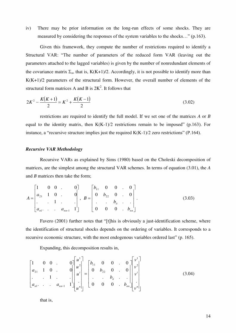
instance, a “recursive structure implies just the required K(K-1)/2 zero restrictions” (P.164).
Recursive VAR Methodology
Recursive VARs as explained by Sims (1980) based on the Choleski decomposition of
matrices, are the simplest among the structural VAR schemes. In terms of equation (3.01), the A
and B matrices then take the form;
1...
..1..
0.01
0.001
11
21
nnn aa
aA ,
nn
ii
b
b
b
b
B
.000
....
0.00
0.00
22
11
. (3.03)
Favero (2001) further notes that “[t]his is obviously a just-identification scheme, where
the identification of structural shocks depends on the ordering of variables. It corresponds to a
recursive economic structure, with the most endogenous variables ordered last” (p. 165).
Expanding, this decomposition results in,
n
i
nn
ii
n
i
nnnv
v
v
v
b
b
b
b
u
u
u
u
aa
a
..000
....
0.00
0.00
.1...
..1..
0.01
0.0012
1
22
112
1
11
21 (3.04)
that is,

15
n
nn
i
ii
n
i
nnnvb
vb
vb
vb
u
u
u
u
aa
a
..1...
..1..
0.01
0.0012
22
1
11
2
1
11
21 (3.05)
Although Sims (1980) used the monetary policy variables first on the assumption that
policy does not respond to the contemporaneous movements in macroeconomic variables
(mainly due to macroeconomic variables being unobserved contemporaneously), later analysts
such as Bernanke and Blinder (1992) have ordered the policy instrument last.
The recursive VAR structure and the notation used by Bernanke and Blinder (1992) are
worth noting as a preamble to introducing the Bernanke-Mihov methodology. Bernanke and
Blinder assume that the “true” economic structure can be written as,
y
t
yk
i
iti
k
i
itit vApCYBY
00
(3.06)
p
t
k
i
iti
k
i
itit vpgYDp
10
(3.07)
where Y represents non-policy variables and p is the policy variable, and A, B,C,D, and g are
relevant matrices and vectors as defined in traditional VAR methodology. To identify this
system econometrically restrictions are needed. Equating D to 0 means that the policy variable is
ordered first since non-policy variables will then, not have a contemporaneous effect on policy.
In a system where i=0,1, this means that
tttt vgpYDp 111 (3.08)
and
ttttt vCupCgCYDCBBIY 01101101
1
0
(3.09)
Alternatively, if C=0, the policy variable would be ordered last, and
tttt upCYBBIY
1111
1
0 (3.10)
and
ttttt uBIDvpCBIDgYBBIDDp1
0011
1
0011
1
001
(3.11)
Bernanke-Mihov Methodology
Bernanke and Blinder’s policy variable p is a scalar measure (i.e., interest rate or interest
rate spread). However, as explained in Section 2, and as Bernanke and Mihov (1998) show “[i]t

16
may be the case that we have only a vector of policy indicators P, which contains information
about the stance of policy” (p.875). If so,
y
t
yk
i
iti
k
i
itit vAPCYBY
10
(3.12)
p
t
pk
i
iti
k
i
itit vAPGYDP
00
(3.13)
With u indicating an (observable) VAR residual and v indicating an (unobservable)
structural disturbance, any policy shock can be measured as,
p
t
pp
t vAGIu1
0
(3.14)
or ignoring the subscripts and superscripts,
AvGuu (3.15)
Bernanke and Mihov (1995) then introduce their ““semi-structural” VAR model which
leaves the relationships among macroeconomic variables in the system unrestricted, but imposes
contemporaneous identification restrictions on a set of variables relevant to the market for
commercial bank reserves” (p.2). Specifically, they use the Federal funds rate, non-borrowed
reserves, borrowed reserves and total reserves in their model of the reserves market. They
assume that one element of the vector vp is a policy disturbance, while it could also include
“shocks to money demand or whatever disturbances affect the policy indicators” (pp.10-11), and
use different restrictions based on various assumptions on the market for commercial bank
reserves to identify policy shocks and their effects on macroeconomic variables.
The relationships between non-policy variables and policy variables in the Bernanke-
Mihov methodology are summarised by De Arcangelis and Di Giorgio (2001). According to
them “[i]n the estimation of the orthogonalized, economically meaningful (structural)
innovations in the second stage, a recursive causal block-order is assumed to form the set of non
policy variables to the set of policy variables. Moreover, the recursive causal order is also
established for the nonpolicy variables in y. In terms of the relationship between the
fundamental innovations, uy and up and the structural innovations vy and vp which are mutually
and serially uncorrelated, this implies
p
y
p
y
v
v
B
B
u
u
AA
A
2,2
1,1
2,21,2
1,1
0
00 (3.16)

17
Where A1,1 is lower-triangular and B1,1 is diagonal so that there is a Wold recursive
(causal) ordering among the nonpolicy variables in y. Moreover, A2,1 is a full matrix so that there
is a Wold block-recursive (causal) ordering between nonpolicy and policy variables” (pp.85-86).
They further explain that “the core of the [Bernanke-Mihov] analysis focuses on the shape that
the matrices A2,2 and B2,2 must take for the different operating procedures to work properly”
(p.86).
Two open economy extensions to the Bernanke-Mihov methodology are provided by De
Arcangelis and Di Giorgio (2001) and Fung (2002). The former consider the exchange rate as a
nonpolicy variable, but since the contemporaneous reaction of the exchange rate to innovations
in the policy variables cannot be excluded, they order it after the policy block. Fung’s (2002)
semi-structural VAR is simpler, and he models the short run monetary policy behaviour and the
foreign exchange market for the analysis of monetary policy in East Asia using the following
two equations:
Interest rate: xs
R vbvu 12 (3.17)
Exchange rate: xs
X vvbu 21 (3.18)
Where vx and v
s represent the exogenous exchange rate and monetary policy shocks,
respectively. Fung shows that “[s]etting b12=0, means that the central bank does not
contemporaneously respond to the exchange rate shock and the innovations in the interest rate
are thus due purely to monetary policy shocks [while] the restriction b21=0 […] implies that the
innovation in the exchange rate does not respond to the interest rate contemporaneously” (p.4).
However, since the policy block has only two variables, this methodology reduces to a recursive
VAR when either restriction advocated by Fung is used.
Deriving a Monetary Policy Index
An important by-product of the Bernanke-Mihov methodology is the derivation of a
monetary policy index. Arguing that “it is also desirable to have indicators of the overall thrust
of policy, including the endogenous or anticipated portion of policy” (p.3), Bernanke and Mihov
(1995) use their semi-structural VAR methodology to derive both measures. They show that an
overall measure of monetary policy derived using their method is similar to a monetary
conditions index “intended to provide assessments of overall tightness or ease, in their day-to-
day policy-making” (Bernanke and Mihov (1998), pp.896-897).

18
Bernanke-Mihov monetary policy index has a simple derivation. From the relationship
given in equation (3.15) and the vector of policy variables P, the following vector of variables
can be obtained
PGIA 1 (3.19)
According to Bernanke and Mihov (1995), these variables, “which are linear
combinations of the policy indicators P, have the property that their orthogonalized VAR
innovations correspond to the structural disturbances v. In particular, one of these variables, call
it p, has the property that its VAR innovations correspond to innovations in the monetary policy
shock” (p.13). They propose using the estimated linear combination of policy indicators p as a
measure of overall monetary policy stance.
Bernanke and Mihov (1998) identify two shortcomings of this measure: “first this
indicator is not even approximately continuous over changes in regime […] Second, this
measure does not provide a natural metric for thinking about whether policy at a given time is
“tight” or “easy”” (p.898). They continue to argue that “a simple transformation of this variable
seems to correct both problems. Analogous to the normalization applied to the reserves
aggregates in the estimation, to construct a final total policy measure we normalize p at each
date by subtracting from it a 36-month moving average of its own past values. This has the
effects of greatly moderating the incommensurable units problem, as well as defining zero as the
benchmark for “normal” monetary policy” (p.898).
Modelling the Policy Block for Sri Lankan Monetary Policy
In the case of Sri Lanka, three time series variables are selected to be included in the
policy block. The first is reserve money (RM), which is the operating target for monetary policy
in Sri Lanka. The second is the interbank call-money market rate (CR) which is an overnight
interest rate closely influenced by CBSL policy action. The third is the exchange rate (Sri
Lankan rupees per SDR) (XRT). The choice of these variables will be discussed in the next
section. However, it should be noted that the inverse of RM and XRT are used in the model, so
that an increase in any variable in the policy block would mean a policy contraction, as
explained at a later point in this analysis. Accordingly, a positive sign in front of NXRT would
mean an appreciation of the Sri Lankan rupee.
The following three equations explain (in innovation terms) the model used for the
present analysis (The derivation is not shown but straight-forward).

19
dNRMNXRTCRNRMvuuu (3.20)
eNXRTCRNXRTvuu (3.21)
seeddCRvvvu (3.22)
Equation (3.20) shows that the demand for RM is negatively related to CR and positively
to an appreciation of the rupee (through its effects on net foreign assets of CBSL). The structural
demand shock is depicted by vd. Equation (3.21) shows that an increase in CR results in an
appreciation of the rupee, while ve represents a structural external shock. Equation (3.22) is
CBSL policy reaction function, and the VAR residual uCR
would include CBSL reaction to
structural demand shocks, structural external shocks, as well as structural monetary policy
innovations.3
Residuals obtained from VAR (u) can then be interpreted as
BvAu1 (3.27)
s
e
d
ed
eNXRTd
eNXRTdNRM
CR
NXRT
NRM
v
v
v
u
u
u
1
(3.36)
Furthermore, structural innovations v, can be isolated as follows:
vAuB 1 (3.44)
CR
NXRT
NRM
NXRT
e
NRM
d
NXRT
e
NRM
d
NRM
d
NXRTNXRT
NRMNRMNRM
s
e
d
u
u
u
v
v
v
1
10
1
(3.51)
The model (3.26) is not identified. The number of restrictions required for just-
identification on A and B matrices is, according to equation (3.02) is
2
1
2
12 22
KK
KKK
K
3 Piffanelli (2001), who uses the Bernanke-Mihov methodology, also employs a policy interest rate, exchange rate
and money supply in the policy block in her study of monetary policy in Germany.

20
=
12392
13332
. (3.55)
whereas there are only 11 restrictions. Just identification can be achieved in the
following ways by imposing one additional restriction:
i) Restricted capital account: This means that the exchange rate does not react to interest
rate innovations, i.e.,
0 (3.56)
Then, the structural shock vs reduces to,
CR
NRM
dNXRT
NXRT
e
NRM
dNRM
NRM
ds
uuuv
1
(3.57)
ii) Fully floating exchange rate regime: This means that the net foreign assets, which is a
part of reserve money remains unchanged, i.e.,
0 (3.58)
Then, the structural innovation becomes
CR
NXRT
e
NRM
dNXRT
NXRT
eNRM
NRM
ds
uuuv
1
(3.59)
iii) Strongin assumption: Following Strongin (1992), Bernanke and Mihov (1995,1998)
assume that reserve money does not react to interest rate innovations
contemporaneously, i.e.,
0 (3.60)
The structural shock then reduces to,
CR
NXRT
eNXRT
NXRT
e
NRM
dNRM
NRM
ds
uuuv
1
(3.61)
However, the need to identify different targeting regimes would mean that the model
may need to be overidentified. Accordingly, the following three targeting regimes are
considered:
i) Interest rate targeting: The imposition of the following two restrictions leads to the
model being overidentified by 1 restriction.

21
0 ed (3.62)
The structural shock then becomes,
CRsuv (3.64)
i.e., the VAR residual uCR
represents the structural shock.
ii) Reserve money targeting: The imposition of the following three restrictions leads to the
model being overidentified by 2 restrictions.
0 and 1NRM (3.65)
Structural innovation vs then reduces to
CR
NXRT
eNXRT
NXRT
eNRMds
uuuv
1
(3.68)
while the innovation to money demand becomes the relevant structural shock.
NRMduv (3.71)
iii) Exchange rate targeting: The following restrictions lead to the model being
overidentified by one restriction.
0 and 1NXRT (3.72)
Structural innovation vs then becomes,
CR
NRM
dNXRTe
NRM
dNRM
NRM
ds
uuuv
1
(3.73)
while the external shock ve becomes the relevant structural shock.
NXRTeuv (3.76)
Deriving a Monetary Policy Index for Sri Lanka
Following equation (3.19), and using the policy block model for Sri Lanka a monetary
policy index can be derived as follows:

22
PAB1
=
CR
NXRT
NRM
NXRT
e
NRM
d
NXRT
e
NRM
d
NRM
d
NXRTNXRT
NRMNRMNRM
1
10
1
CRNXRTNRMNXRT
e
NRM
d
NXRT
e
NRM
d
NRM
d
1
(3.77)
As explained by Bernanke and Mihov (1995, 1998), the monetary policy measure so
derived is a linear combination of all variables in the monetary policy block and is a useful index
for observing the direction of monetary policy.
Data Description
The main data sources in this analysis are the IMF’s International Financial Statistics and
the publications of Central Bank of Sri Lanka. Although many data series required are available
from 1950s, this study uses data since 1978 in order to focus on the effects of Sri Lanka’s
monetary policy in an open economy framework.
Table 1
Data Series Used in the Analysis
Series Units Source Remarks
Gross Domestic
Product at 1996
Constant Factor
Cost Prices
(GDPSA)
Sri Lankan Rupees
Million
Base year=1996
CBSL-Annual Reports
and GDP Press
Releases
Interpolated from Annual series for
the period from 1978-1995 and from
Quarterly Seasonally adjusted series
from 1996-2005
Colombo
Consumers’ Price Index
(CCPISA)
Units: Index No
Base year=2000
(=100)
IFS
Line 64...ZF
CPI:COLOMBO 455
MNUAL WRKRFAM
Seasonally adjusted using Census
X-12 ARIMA
SDR Exchange
Rate
(XRTSDRAVGSA)
Sri Lankan Rupees
per SDR
IFS
Line ..AA.ZF
MARKET RATE
Monthly Average
Seasonally adjusted using Census
X-12 ARIMA
Reserve Money
(RMSA)
Sri Lankan Rupees
Million
IFS
Line 14...ZF
RESERVE MONEY
End Period
Seasonally adjusted using Census
X-12 ARIMA
Interbank Call
Money Market rate
(CALLRTSA)
Percentage points
IFS
Line 60B..ZF
INTERBANK CALL
LOANS
End period
Seasonally adjusted using Census
X-12 ARIMA

23
The key non-policy variables that will be used are real gross domestic product (GDP)
and consumer price level (CPI). Similar to the case of other economies as explained earlier, one
faces some difficulty in choosing a suitable monetary policy variable in the context of Sri Lanka.
Potential monetary policy indicators can be categorised under three broad classes, namely,
monetary aggregates, interest rates, or exchange rate.
Of the monetary aggregates, reserve money, which is the operating target of monetary
policy implementation and closely monitored by the Central Bank on a weekly basis, is a
preferred candidate over the narrow money (M1) or broad money (M2 or M2b) aggregates.
Although the Repo rate and the reverse Repo rate (and earlier the bank rate) are the direct
policy instruments, these do not span over the full sample. For instance the active use of the
bank rate was discontinued in 1985, while the Repurchase rate was introduced only in 1993.
However, the interbank call money market rate, which is not a policy variable per se, is an
overnight interest rate closely monitored by the Central Bank while Central Bank policy actions
are swiftly reflected in the changes in this rate. This suggests that the interbank call money
market rate could be used as an appropriate indicator of monetary policy.
Finally, since the exchange rate has been a managed float through the most of the sample
period, it also has the potential of being used as a monetary policy indicator. Although the
exchange rate was floated in 2001, being a small open economy with heavy trade dependency,
the exchange rate still attracts much attention in monetary policy discussions, which justify its
use as a monetary policy variable in the present analysis. Also, as Fung (2002) states in the
context of East Asian economies “[t]he exchange rate channel is one of the key channels of
monetary transmission. A contractionary monetary policy leads to an appreciation of the local
currency, which in turn will reduce exports and exert downward pressure on inflation. The
currency appreciation will also reduce domestic inflation through lower import prices. The more
open the economy, the more important the exchange rate channel” (p.2).
All series used are monthly. Since a monthly real GDP or aggregate production series is
not available, the annual series (and the quarterly series from 1996) is interpolated using the
Goldstein and Khan (1976) method.4 Using monthly series is important since the identifying
assumption of there being “no feedback from policy variables to the economy within the period
[…] or the alternative assumption that policy-makers do not respond to contemporaneous
4 Attempts to assess the effects of monetary policy in Sri Lanka face a major drawback as a long time series of high
frequency aggregate production is not available. However, several methods exist to derive high frequency (e.g.
monthly) data series from available low frequency (e.g. Annual or Quarterly) data series and the method introduced
by Goldstein and Khan (1976) is used in the current analysis.
24
information” cannot be defended if one uses quarterly or annual data. (Bernanke and Mihov
(1995), pp.19-20) Also, as IMF (2004) states, “[w]hile the CBSL does not observe GDP
contemporaneously (within a quarter) when deciding on interest rates, they do observe variables
strongly correlated with it – such as rainfall, government revenue, exports, or industrial
production; data on prices and reserve money, which is strongly correlated with broad money,
are available with a very short lag” (p.7, n.).
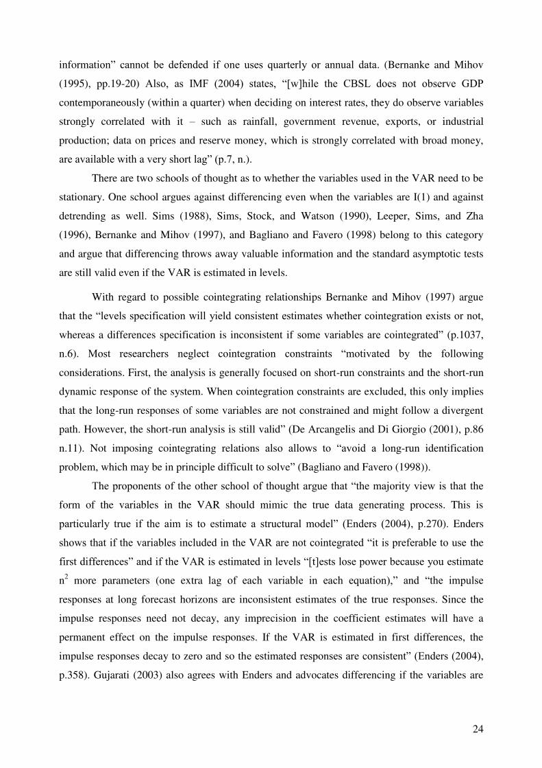
There are two schools of thought as to whether the variables used in the VAR need to be
stationary. One school argues against differencing even when the variables are I(1) and against
detrending as well. Sims (1988), Sims, Stock, and Watson (1990), Leeper, Sims, and Zha
(1996), Bernanke and Mihov (1997), and Bagliano and Favero (1998) belong to this category
and argue that differencing throws away valuable information and the standard asymptotic tests
are still valid even if the VAR is estimated in levels.
With regard to possible cointegrating relationships Bernanke and Mihov (1997) argue
that the “levels specification will yield consistent estimates whether cointegration exists or not,
whereas a differences specification is inconsistent if some variables are cointegrated” (p.1037,
n.6). Most researchers neglect cointegration constraints “motivated by the following
considerations. First, the analysis is generally focused on short-run constraints and the short-run
dynamic response of the system. When cointegration constraints are excluded, this only implies
that the long-run responses of some variables are not constrained and might follow a divergent
path. However, the short-run analysis is still valid” (De Arcangelis and Di Giorgio (2001), p.86
n.11). Not imposing cointegrating relations also allows to “avoid a long-run identification
problem, which may be in principle difficult to solve” (Bagliano and Favero (1998)).
The proponents of the other school of thought argue that “the majority view is that the
form of the variables in the VAR should mimic the true data generating process. This is
particularly true if the aim is to estimate a structural model” (Enders (2004), p.270). Enders
shows that if the variables included in the VAR are not cointegrated “it is preferable to use the
first differences” and if the VAR is estimated in levels “[t]ests lose power because you estimate
n2 more parameters (one extra lag of each variable in each equation),” and “the impulse
responses at long forecast horizons are inconsistent estimates of the true responses. Since the
impulse responses need not decay, any imprecision in the coefficient estimates will have a
permanent effect on the impulse responses. If the VAR is estimated in first differences, the
impulse responses decay to zero and so the estimated responses are consistent” (Enders (2004),
p.358). Gujarati (2003) also agrees with Enders and advocates differencing if the variables are
25
non-stationary. The price for transforming data by first-differencing is however, as Harvey
(1990) notes, the results being not as satisfactory as using levels.
In the present analysis, the latter method is used and appropriate transformations will be
used if some variables are found to be non-stationary.
Descriptive Statistics and Unit Root Tests
Unit root tests confirm that while the interest rate (CALLRTSA) is stationary at the 5 per
cent level of significance, all other variables become stationary only after a log- difference
transformation. That is, CALLRTSA is I(0) while the other series under consideration are I(1).
Although the I(1) variables may be cointegrated, since the interest rate, which is of primary
importance, is I(0) and because estimating long run equilibrium relationships are not the primary
objective of the present analysis, CALLRTSA will be used in levels, while the other series are
transformed by taking log-differences. 5
The descriptive statistics of the final data series used in the analysis after required
transformations for the full Sample are given in Table 2. The logarithmic difference
transformation of GDP, CPI, reserve money, and exchange rate also allow the series to be
interpreted as GDP growth, inflation, reserve money growth and exchange rate depreciation in
percentage points. Note that none of the series used as well as the results obtained is annualised.
Table 2 shows that, on average, GDP has grown by around 0.4 per cent per month, while
prices have increased by around 0.9 per cent monthly. As observed by IMF (2004), “[r]eserve
money has grown on average by less than broad money as reserve requirements have declined
gradually”, but broad money growth is “entirely consistent with the quantity theory and a very
5 Also, as Lütkepohl (2004) notes, cointegration analysis is sometimes used even if the system has both I(1) and I(0)
variables “by calling any linear combination that is I(0) a cointegration relation, although this terminology is not in
the spirit of the original definition because it can happen that a linear combination of I(0) variables is called a
cointegration relation” (p.89).
Table 2
Descriptive Statistics of Data Series after Required Transformations
DLGDPSA DLCCPISA DLRMSA DLXRTSDRSA CALLRTSA
Mean 0.0039 0.0090 0.0115 0.0061 0.1827
Median 0.0041 0.0089 0.0112 0.0050 0.1636
Maximum 0.0136 0.0808 0.0989 0.0879 0.7988
Minimum -0.0136 -0.0357 -0.1613 -0.0614 0.0785
Std. Dev. 0.0030 0.0121 0.0232 0.0176 0.0835
Observations 335 335 335 335 336

26
small decline in the velocity of money” (pp.4-5). Although, the present study covers a longer
period than IMF (2004), their observations seem to apply for this study as well. The Sri Lankan
rupee has depreciated against SDR by around 0.6 per cent per month, while the call rate has
been, on average, around 18 per cent. All variables, perhaps except for GDP growth, show
considerable volatility.
IV: Analysis
This section begins with estimating a series of recursive VAR specifications. The semi-structural
VAR methodology explained in section III will then be executed and its results will be analysed.
Finally, a monetary policy index is derived using the estimated semi-structural VARs.
A clarification is needed with regard to a simple transformation of reserve money growth
and exchange rate depreciation series used in the analysis. An increase in the interest rate
(CALLRTSA) can be obviously treated as a monetary policy contraction. However, an increase
in the exchange rate (DLXRTSDRAVGSA), as defined in the data description in section III,
indicates exchange rate depreciation, while an increase in the series DLRMSA shows a positive
money growth. Both exchange rate depreciation and positive money growth have expansionary
effects on output and prices. To bring the latter two series in line with the interest rate, they are
redefined by inverting. That is, using the negative of reserve money growth (NRM) and the
negative of exchange rate depreciation (NXRT), i.e., exchange rate appreciation, would allow
increases in all three series in the policy block to be treated as contractionary shocks. These
modified series will be used in the analysis hereafter. Note that the modified definitions were
also used in the derivation of the model for the policy block in section III.
Recursive VAR Estimates
The first recursive VAR to analyse is a model with real GDP, inflation, negative of
reserve money growth, exchange rate appreciation, and call rate, in that order. The choice of the
order indicates that the last three variables, which are generally considered as policy variables in
the present analysis are informed contemporaneously by the macroeconomic variables of GDP
growth and inflation. Innovations in policy variables do not affect the macroeconomic variables
contemporaneously. The recursive structure employed assumes that the call rate is the most
endogenous variable since it is affected contemporaneously by the innovations of reserve money
and exchange rate but not vice versa. The ordering of reserve money and exchange rate cannot
27
be theoretically explained, but a different ordering of these two variables do not affect the results
of the analysis significantly.
Lag length selection criteria are considered in determining a suitable number of lags to
be included in the specification. Schwartz and Hannan-Quinn criteria select a short lag length of
one lag, while Akaike criterion selects seven lags. The likelihood ratio statistic prefers a longer
lag length and recommends the selection of 19 lags. Considering these criteria and the fact that
the analysis employs monthly series, an interim approach of using 12 lags is utilised.
However, Wald tests of the null hypotheses of the possibility of exclusion reveal that
some interim lags within the 12-lagged specification may be unimportant. Accordingly, only
lags 1, 2, 4, 5, 6 and 12 which are significant at standard levels of significance are used in this
recursive VAR.
The specification satisfies the stability properties as shown in Figure 4.1, since all
inverse roots of the characteristic polynomial lie inside the unit circle as explained by Lütkepohl
(1993) among others.
Mainly due to the use of log differences in the analysis, the goodness of fit is affected. In
particular, the exchange rate equation has very low adjusted R2 and F-statistics. R
2 and F-
statistics improve significantly when recursive VARs with the same specification is used in log
levels. However, due to the reasons given in Section 3, stationary variables are used in the
current VAR analysis.
Table 3 (Summary)
Recursive VAR – Full Sample
Vector Autoregression Estimates
Sample (adjusted): 1979M02 2005M12
Included observations: 323 after adjustments
DLGDP DLCCPI NDLRM NDLXRTSDR CALLRT
R-squared 0.408577 0.175883 0.194516 0.113073 0.676403
Adj. R-squared 0.347815 0.091214 0.111761 0.021950 0.643157
Sum sq. resids 0.001752 0.036481 0.141684 0.086364 0.723303
S.E. equation 0.002450 0.011177 0.022028 0.017198 0.049770
F-statistic 6.724157 2.077289 2.350501 1.240889 20.34525
Log likelihood 1499.806 1009.495 790.3701 870.3162 527.0879
Akaike AIC -9.094771 -6.058794 -4.701982 -5.197005 -3.071752
Schwarz SC -8.732210 -5.696232 -4.339421 -4.834444 -2.709191
Mean dependent 0.003795 0.008893 -0.011705 -0.006109 0.186183
S.D. dependent 0.003033 0.011725 0.023372 0.017390 0.083316

28
The impulse responses obtained from the first recursive VAR show that as a result of a
one standard deviation shock of the policy rate GDP growth rate falls by around 0.02 per cent
each month for about a year with the peak effect in the fifth month following the shock. The
peak effect of an interest rate shock on inflation occurs in the third month following the shock
with inflation decreasing by around 0.1 per cent. However, the effect on inflation is short-lived
and the reduction in inflation reverses after 6 months. The effect of a positive innovation of
interest rate on reserve money is unclear. Although the exchange rate depreciates for about four
months following an interest rate increase, it is followed by a continuous appreciation till the
13th
month by around 0.05 per cent each month. The increase in the interest rate dies out only
gradually indicating further tightening of monetary policy that follows an initial tightening.
A one standard deviation exchange rate appreciation has a positive effect on GDP which
is counter-intuitive, but it has a significant effect on reducing inflation, with inflation decreasing
by 0.15 per cent in the third month following the shock. Interest rate responds to a one standard
deviation exchange rate appreciation immediately by reducing the interest rate by around 0.75
per cent for two months.
Innovations in reserve money growth do not show any significant result, perhaps because
the inclusion of an interest rate absorbs the predictive power of reserve money.
In respect of accumulated responses, it can be seen that a one standard deviation
innovation to the interest rate reduces GDP growth by a total of around 0.2 per cent within a
year and the output growth recovers only gradually. The accumulated negative effect on
inflation totals 0.2 per cent after 6 months, and the accumulated impact remains positive from 9
months onwards. Reserve money increases at first, but the accumulated result is a decline in
reserve money. Similarly, following a brief depreciation of the exchange rate, the accumulate
effect is a continuous appreciation.
GDP growth remains positive following an exchange rate appreciation, which is a
counter-intuitive result. Inflation declines throughout as a result of an appreciation. An exchange
rate innovation (appreciation) leads to the interest rate declines for a long period.
Variance decompositions show that own variance is very important with respect to all
variables while monetary policy indicators contribute very little in explaining variance of non
policy variables. Perhaps the only exception is the percent call rate variance due to inflation
which is about 15 per cent. Following Bernanke and Mihov (1995, 1998) variance
decompositions will be largely ignored in the ensuing discussion.

29
Table 4.1
Recursive VAR-Full Sample
Direction of Responses to a Contractionary Interest Rate Shock
Variable Expected
Observed
On Impact Peak Accumulated
GDP ↓ ↓ ↓(5) ↓
CPI ↓ ↓ ↓(3), ↑(7) ↑
NRM ↑ ↓ ↑(6) ↑
NXRT ↑ ↓ ↑(5) ↑
IR ↑ ↑ ↑ ↑
Table 4.2
Recursive VAR-Full Sample
Direction of Responses to a Contractionary Exchange Rate Shock (Appreciation)
Variable Expected
Observed
On Impact Peak Accumulated
GDP ↓ ↑ ↑(3) ↑
CPI ↓ ↓ ↓(2) ↓
NRM Ambiguous ↓ ↓(3), ↑(13) ↓
NXRT ↑ ↑ ↑ ↑
IR ↓ ↓ ↓(1) ↑
Table 4.3
Recursive VAR-Full Sample
Direction of Responses to a Contractionary Reserve Money Shock
Variable Expected
Observed
On Impact Peak Accumulated
GDP ↓ ↑ ↓(6) ↓
CPI ↓ ↓ ↑(5) None
NRM ↑ ↑ ↑ ↑
NXRT None ↑ ↓(3) ↓
IR ↑ ↓ ↑(5) None
Notes:
1. Expected column indicates the expected direction at the peak.
2. On impact column indicates the direction of the first available response.
4. In the peak column, the number within parenthesis is the lag of the peak response.
3. Accumulated column indicates the direction of accumulated response after 36 months.
The summary provided in Table 4 assesses the results obtained from the first recursive
VAR against expected results. Results are broadly in line with consensus views when an interest
rate innovation is considered. However, exchange rate and reserve money innovations provide
some puzzling results.
Since the full sample from January 1978 to December 2005 is marked with several
important monetary policy changes, the first recursive VAR specification is tested using several
sub-samples to see whether results obtained for the full sample change for sub-samples. The
determination of sub-samples is as follows:

30
Table 5
Determination of Sub-samples
Sample Period Reason
January 1978-December 2005 Full sample
January 1978-September 1993 Period covers from the beginning of the sample up to the introduction of
the Repo rate
October 1993-December 2000 Period covers from the introduction of the Repo rate up to the floating of
the exchange rate
January 2001-December 2005 Period covers from the floating of the exchange rate up to the end of the
sample period
The sub-samples fail to improve the ambiguous results obtained from the full sample
relating to both reserve money and exchange rate, while recent sub-samples are plagued with the
perverse seasonality problem caused by the behaviour of the real GDP series. Standard errors of
all impulse responses are high, questioning the statistical significance of the findings. However,
some common patterns can be observed from the above results. Innovations to the interest rate
reduce GDP growth. The response of inflation to an interest rate shock is often positive.6 The
increase in inflation following an interest rate innovation is the price puzzle and the inclusion of
crude oil prices does not provide a solution, as in the case of Fung (2002) who finds that
“[i]ncluding the commodity price index or US variables in the VARs, however, does not resolve
this price puzzle” (pp.7-8) for many East Asian economies.
The relationship between interest rates and exchange rate appreciation is positive, as
expected. The persistence of interest rate innovations suggests that CBSL changes interest rate
gradually, and confirms an earlier finding of IMF (2004) for Sri Lanka. Contractionary exchange
rate innovations (appreciations) result in increasing GDP growth at all times. This is somewhat
surprising given the export-oriented nature of Sri Lanka’s economy where one expects an
exchange rate appreciation to discourage exports and thereby reduce GDP growth. IMF (2004)
also finds that “[a]n unexpected depreciation […] is associated with a significant decline in
output, which suggests that such an innovation may be a proxy for some underlying
macroeconomic weakness” (p.11). Innovations in reserve money growth do not lead to
significant findings, and the reserve money contractions and interest rates often have a negative
relationship, giving rise to what Leeper, Sims, and Zha (1996) called the liquidity puzzle. Fung
(2002) also finds a similar puzzling result for Korea.
6 IMF (2004) also finds that in Sri Lanka, “changes in policy interest rate have a significant effect on output but a
small impact on inflation. […] Inflation in Sri Lanka is very volatile and the effect of monetary shocks is dwarfed by supply-side shocks, in particular to agricultural production given the large weight of food in the CPI. […] Since the weight of food in the price index is about 2/3, it is not surprising that the link between monetary policy shocks
and inflation is weak” (pp.9-11).

31
Although the theory dictates that monetary policy does not have a long run impact on
GDP, accumulated responses of GDP growth die out only sluggishly in most occasions.
The next section employs the Bernanke-Mihov methodology instead of recursive VAR
methodology to assess whether impulse responses generated from structural VARs provide
different results to the ones obtained in the present section.
Semi Structural VAR estimates
As explained in detail in Sections II and III, recursive VARs generally assume that a
good scalar policy variable is available, and obtain impulse responses by ordering the policy
variable last. However, the recursive VARs discussed in previous section showed that as in
many other economies, in Sri Lanka also there is a vector of potential policy indicators and one
may need to assess the impact of all these policy variables on macroeconomic variables
simultaneously. Such a requirement can be met by utilising the Bernanke-Mihov methodology
as described in the relationships described in equations (3.20) through (3.22) in Section III.
Accordingly, this section estimates the structural VARs for several sub-samples. The estimates
of the structural VARs with different identification schemes will then be compared.
Just Identified Structural VAR (SVAR-JI)
The first Structural VAR that will be estimated is a just-identified specification for the
full sample period. As described in Section III, there are several ways to achieve just-
identification, and the restriction 0 (equation 3.56) which means that the exchange rate
does not react to interest rate innovations contemporaneously will be utilised in this analysis.
The analysis of impulse responses shows that GDP growth and inflation decline
following a structural interest rate innovation. The reaction of reserve money growth to an
interest rate innovation is still ambiguous, although reserve money growth is negative initially.
The exchange rate initially depreciates, but is followed by a continuous appreciation as a result
of an interest rate shock. An appreciation of the exchange rate (positive innovation), raises GDP
growth, while reducing inflation. A contractionary reserve money growth shock also raises GDP
growth while reducing inflation in the very short-run.

32
The results of the impulse response analysis are summarised in Table 6.
Table 6.1
Structural VAR-JI – Full Sample
Direction of Responses to a Contractionary Interest Rate Shock
Variable Expected Observed
On Impact Peak Accumulated
GDP ↓ ↑ ↓(5) ↓
CPI ↓ ↓ ↓(3), ↑(7) ↑
NRM ↑ ↑ ↑(1) ↑
NXRT ↑ ↓ ↓ (3) ↑
IR ↑ ↑ ↑ ↑
Table 6.2
Structural VAR-JI – Full Sample
Direction of Responses to a Contractionary Exchange Rate Shock (Appreciation)
Variable Expected Observed
On Impact Peak Accumulated
GDP ↓ ↑ ↑(3) ↑
CPI ↓ ↓ ↓(2) ↓
NRM Ambiguous ↑ ↓(3) ↑
NXRT ↑ ↑ ↑ ↑
IR ↓ ↓ ↓(1) ↓
Table 6.3
Structural VAR-JI – Full Sample
Direction of Responses to a Contractionary Reserve Money Shock
Variable Expected Observed
On Impact Peak Accumulated
GDP ↓ ↑ ↓(6) ↓
CPI ↓ ↓ ↑(5) ↓
NRM ↑ ↑ ↑ ↑
NXRT None ↓ ↓(3) ↓
IR ↑ ↓ ↓ (1) ↓
Notes:
1. Expected column indicates the expected direction at the peak.
2. On impact column indicates the direction of the first available response.
4. In the peak column, the number within parenthesis is the lag of the peak response.
3. Accumulated column indicates the direction of accumulated response after 36 months.
The structural VAR results for the sub-sample from January 1978 to September 1993 are
comparable with the recursive VAR for the same sub-sample. As a result of a positive interest
rate innovation, both GDP growth and inflation increases initially, but inflation starts to fall
significantly after nine months for about a further year. Exchange rate appreciates, in general,
after an interest rate shock. Following an exchange rate appreciation, GDP growth rises, while
inflation falls on impact. Interest rate decreases, while the exchange rate innovation shows no
sign of persistence. A negative innovation in reserve money growth has a lagged effect on

33
reducing GDP growth, while inflation starts to decreases four months after the shock. The
puzzling result of interest rate falling after a negative reserve money growth is observed again.
As noted earlier, the sub-sample from October 1993 to December 2000 is marked by the
volatility of responses with the seasonality effect of GDP. Following an interest rate innovation
both GDP growth and inflation fall, although inflation begins to increase seven months after the
shock. Exchange rate appreciates while interest rate innovations are less persistent disappearing
six months after an innovation. As a result of a contractionary exchange rate shock, GDP growth
increases, inflation falls, while interest rate decreases. A contractionary reserve money shock
raises GDP growth but inflation initially falls. Interest rate increases as expected, while reserve
money shocks are less persistent in this sub-sample.
The sub-sample from January 2001 to December 2005 is also plagued with the
seasonality effect. Although innovations to interest rate and reserve money cause expected
negative result on GDP growth, exchange rate shocks continue to affect GDP growth positively.
Interest rate innovations do not help reduce inflation. Exchange rate appreciates following an
interest rate shock, while CBSL appears to have changed interest rates gradually, both in terms
of magnitude and length of adjustment. Another significant result is that interest rate rises
following a negative innovation in reserve money growth similar to the previous sub-sample.
General Discussion on Structural VAR Results
The results obtained from the just-identified structural VARs are not quite different to
the results of recursive VARs. The only puzzle that is resolved is the liquidity puzzle, since in
two sub-samples interest rate rises following a contractionary reserve money shock. Monetary
policy still appears to have little impact on reining-in inflationary pressures while exchange rate
appreciation has a counter-intuitive positive impact on GDP growth.
A logical next-step is to test whether the various sub-samples can be identified as
different targeting regimes. Accordingly, restrictions 0 ed given in equation (3.62) is
used to derive estimates under an interest rate targeting regime, restrictions 0 and
1NRM as in equation (3.65) are utilised to obtain estimates under a reserve money targeting
regime. An exchange rate targeting regime is defined by 0 and 1NXRT as in equation
(3.72). A summary of the results obtained are provided in Table 7.
A comparison of the parameter estimates shows that parameters are broadly consistent
within each sample. Also, most parameters carry the expected sign. Parameter from equation

34
(3.20) is the elasticity of (negative) of reserve money growth to interest rate and is expected to
have a positive sign. For the full sample as well as all sub-samples this is estimated to be
positive. It is also observed that for the sub-sample from January 2001 to December 2005, this
parameter is significantly higher than in other sub-samples. Parameter , which is the elasticity
of (negative of) reserve money growth to an exchange rate appreciation, does not carry the
expected negative sign for the two sub-samples from October 1993 to December 2000, and
January 2001 to December 2005. However, through all samples parameter is statistically
insignificant. Parameter shows the effect of interest rate on the exchange rate. This parameter
has the expected positive values in all estimates and in the most recent sub-sample has a large
and significant value perhaps indicating the impact of the gradual capital account liberalisation
that has been taking place in recent times. Parameters NRM and NXRT
, which show the reaction
of (negative of) reserve money and exchange rate to demand and external shocks, respectively,
have positive signs as expected. Parameters d and e
, which show the reaction of the interest
rate to demand innovations and external shock, respectively, change signs throughout samples
displaying that interest rates have reacted differently to shocks at different times. The analysis of
overidentifying restrictions proves futile since all overidentifying restrictions are rejected by the
model,7 possibly indicating that any sub-sample in the post-1978 monetary history of Sri Lanka
cannot be identified with one targeting regime. CBSL has paid attention to all three policy
variables included in the model in the conduct of monetary policy and VAR estimates using
different identification schemes are unlikely to improve the results obtained from the just-
identified models any further.
7 Bernanke and Mihov (1995) advocates that since tests for overidentifying restrictions “gives only the statistical,
and not economic, significance of model rejections…an alternative strategy is to […] get just-identification; and
then, conditional on that restriction, to observe how closely the estimated parameter values of the more general
model correspond to those assumed by the more restricted models” (p.26), as performed in the current analysis.

35
Table 7
Parameter Estimates for All Structural VAR Models
Sample Model NRM NXRT d e Log
likelihood
1979M02
-2005M12
(Full
Sample)
JI-1 0.0454
[0.9978]
-0.0993
[0.9908] 0
0.0217
[0.0000]
0.0171
[0.0000]
0.0000
[1.0000]
-0.0090
[0.8719] 3814.6
IRT 0.0466
[0.0000]
-0.0988
[0.1683]
0.0625
[0.0000]
0.0217
[0.0000]
0.0168
[0.0000] 0 0 3820.0
RMT 0 0 0.0608
[0.0323] 1
0.0168
[0.0000]
-0.0330
[0.5537]
0.0000
[1.0000] 2744.0
XRTT 0.0456
[0.9833]
-0.0973
[0.9315] 0
0.0217
[0.0000] 1
0.0004
[1.0000]
-0.5207
[0.0000] 2661.9
1979M02
-1993M09
JI-1 0.0470
[0.9846]
-0.0232
[0.9795] 0
0.0180
[0.0000]
0.0175
[0.0000]
-0.0004
[1.0000]
-0.0065
[0.9317] 2234.8
IRT 0.0547
[0.0000]
-0.0212
[0.7870]
0.0767
[0.0000]
0.0180
[0.0000]
0.0173
[0.0000] 0 0 2237.3
RMT 0 0 0.0647
[0.0653] 1
0.0173
[0.0000]
0.0371
[0.6224]
-0.0006
[0.9998] 1618.4
XRTT 0.0514
[0.9908]
-0.0214
[0.9896] 0
0.0180
[0.0000] 1
0.0002
[1.0000]
-0.3686
[0.0000] 1611.0
1993M10
-2000M12
JI-1 0.0745
[0.9907]
0.0054
[0.9996] 0
0.0298
[0.0000]
0.0135
[0.0000]
0.0004
[0.0000]
-0.0248
[0.8170] 1007.0
IRT 0.0720
[0.0000]
0.0010
[0.9969]
0.0608
[0.0000]
0.0298
[0.0000]
0.0128
[0.0000] 0 0 1012.1
RMT 0 0 0.0610
[0.0000] 1
0.0128
[0.0000]
-0.3329
[0.0019]
0.0000
[1.0000] 749.9
XRTT 0.0719
[0.9973]
0.0054
[0.9999] 0
0.0298
[0.0000] 1
0.0001
[1.0000]
-1.7576
[0.0000] 676.2
2001M01
-2005M12
JI-1 0.1398
[0.9359]
0.0529
[0.7585] 0
0.0163
[0.0000]
0.0196
[0.0000]
-0.0009
[1.0000]
-0.0015
[0.9906] 705.7
IRT 0.3240
[0.0000]
0.0732
[0.5020]
0.4400
[0.0000]
0.0162
[0.0000]
0.0192
[0.0000] 0 0 707.4
RMT 0 0 0.1034
[0.4288] 1
0.0194
[0.0000]
-0.0192
[0.8819]
-0.0008
[0.9999] 489.2
XRTT 0.1428
[0.9433]
0.0523
[0.7385] 0
0.0163
[0.0000] 1
-0.0007
[1.0000]
-0.0780
[0.5457] 499.8
Note: P-values are in parentheses
Estimating the Monetary Policy Index
Using the methodology explained in Section III and based on equation (3.77), an attempt
is made to derive a monetary policy index for Sri Lanka. Although many authors, including
Bernanke and Mihov (1995, 1998), and Kasa and Popper (1997) have used the parameter
estimates from the just-identified model for the full sample to derive such an index, in this
analysis, it is proposed to use an average of parameter estimates (ignoring restricted values) to
derive the index. Although, parameter estimates are roughly equal within a sample as already
mentioned, taking average values further helps to avoid estimating an index biased toward any
particular identifying assumption. The average parameter values for the full sample are as
follows:
36
Table 8
Parameter Values used for the Monetary Policy Index
0.0459
-0.0985
0.0616
NRM 0.2170
NXRT 0.0169
d -0.0109
e -0.1766
The estimated monetary policy index is displayed in Figure 1. As suggested by
Bernanke and Mihov (1995), policy variables are transformed by subtracting them from their
own 36-month moving averages before estimating the monetary policy index given by equation
(3.77). The estimated parameter values determine the weight on each policy variable, and as
expected from the foregoing impulse response analyses, the interest rate has a greater weight
than reserve money and the exchange rate. This makes the three policy variables to have
comparable units and defined the zero line as “normal” monetary policy.8 When the index is
above the zero line, it can be interpreted as a contractionary monetary policy stance, and vice
versa.
Figure 13
Monetary Policy Index for Sri Lanka
-0.30
-0.20
-0.10
0.00
0.10
0.20
0.30
0.40
0.50
0.60
19
81
M0
4
19
82
M0
4
19
83
M0
4
19
84
M0
4
19
85
M0
4
19
86
M0
4
19
87
M0
4
19
88
M0
4
19
89
M0
4
19
90
M0
4
19
91
M0
4
19
92
M0
4
19
93
M0
4
19
94
M0
4
19
95
M0
4
19
96
M0
4
19
97
M0
4
19
98
M0
4
19
99
M0
4
20
00
M0
4
20
01
M0
4
20
02
M0
4
20
03
M0
4
20
04
M0
4
20
05
M0
4
Un
its
8 Bernanke and Mihov warn that the index defines “normal” monetary policy compared with the recent past. Kasa
and Popper (1997) concur: “since only second moments are being used here, these plots cannot say anything about the stance of policy in some absolute sense. Only the stance of policy relative to the historical average is identified” (p.291 n.26).
Figure 1

37
Figure 2 plots the estimated structural monetary policy shocks (vs) obtained from the
model with a similar transformation to make it comparable with Figure 1. Structural monetary
policy shocks can be defined as the unanticipated monetary policy. According to Kasa and
Popper (1997) who estimate a similar index for Japan, [t]he overall stance reflects both
endogenous responses to economic conditions and unanticipated changes in the stance of
policy” (p. 291). Similar to their observation for Japan, in Sri Lanka also the unanticipated
component of monetary policy is relatively small compared with the overall stance of monetary
policy. Kasa and Popper, interpret this observation as indicating “that the recent, striking
changes in the stance of Japanese monetary policy took place largely in response to the
prevailing economic condition” (p.292). This interpretation is applicable to Sri Lanka as well.
For instance, even the high interest rate regime observed during the late 1995, it has largely been
in response to the existing economic situation of the country.
Figure 14
Estimated Structural Monetary Policy Shocks (Unanticipated)
-0.30
-0.20
-0.10
0.00
0.10
0.20
0.30
0.40
0.50
0.60
19
81
M0
4
19
82
M0
4
19
83
M0
4
19
84
M0
4
19
85
M0
4
19
86
M0
4
19
87
M0
4
19
88
M0
4
19
89
M0
4
19
90
M0
4
19
91
M0
4
19
92
M0
4
19
93
M0
4
19
94
M0
4
19
95
M0
4
19
96
M0
4
19
97
M0
4
19
98
M0
4
19
99
M0
4
20
00
M0
4
20
01
M0
4
20
02
M0
4
20
03
M0
4
20
04
M0
4
20
05
M0
4
Un
its
The difference between the monetary policy index and exogenous shocks provides the
endogenous responses of monetary policy to the current economic condition, and are presented
in Figure 3.
Figure 2
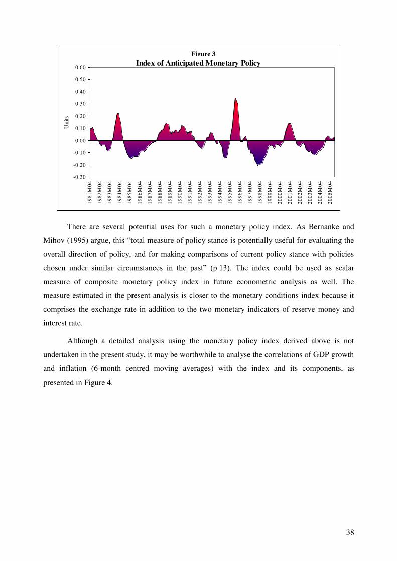
38
Figure 15
Index of Anticipated Monetary Policy
-0.30
-0.20
-0.10
0.00
0.10
0.20
0.30
0.40
0.50
0.60
19
81
M0
4
19
82
M0
4
19
83
M0
4
19
84
M0
4
19
85
M0
4
19
86
M0
4
19
87
M0
4
19
88
M0
4
19
89
M0
4
19
90
M0
4
19
91
M0
4
19
92
M0
4
19
93
M0
4
19
94
M0
4
19
95
M0
4
19
96
M0
4
19
97
M0
4
19
98
M0
4
19
99
M0
4
20
00
M0
4
20
01
M0
4
20
02
M0
4
20
03
M0
4
20
04
M0
4
20
05
M0
4
Units
There are several potential uses for such a monetary policy index. As Bernanke and
Mihov (1995) argue, this “total measure of policy stance is potentially useful for evaluating the
overall direction of policy, and for making comparisons of current policy stance with policies
chosen under similar circumstances in the past” (p.13). The index could be used as scalar
measure of composite monetary policy index in future econometric analysis as well. The
measure estimated in the present analysis is closer to the monetary conditions index because it
comprises the exchange rate in addition to the two monetary indicators of reserve money and
interest rate.
Although a detailed analysis using the monetary policy index derived above is not
undertaken in the present study, it may be worthwhile to analyse the correlations of GDP growth
and inflation (6-month centred moving averages) with the index and its components, as
presented in Figure 4.
Figure 3

39
Fig
ure 4
D
yn
am
ic Co
rrelatio
ns b
etween
the M
on
etary
Policy
Ind
ex a
nd
Macro
econ
om
ic Varia
bles
DL
GD
P
-0.3
-0.2
-0.1 0
0.1
0.2
0.3
MPI(-36)
MPI(-33)
MPI(-30)
MPI(-27)
MPI(-24)
MPI(-21)
MPI(-18)
MPI(-15)
MPI(-12)
MPI(-9)
MPI(-6)
MPI(-3)
MPI
DL
CC
PI
-0.3
-0.2
-0.1 0
0.1
0.2
0.3
MPI(-36)
MPI(-33)
MPI(-30)
MPI(-27)
MPI(-24)
MPI(-21)
MPI(-18)
MPI(-15)
MPI(-12)
MPI(-9)
MPI(-6)
MPI(-3)
MPI
Fig
ure 4
.1.1
F
igu
re 4.2
.1
DL
GD
P
-0.3
-0.2
-0.1 0
0.1
0.2
0.3
EXO(-36)
EXO(-33)
EXO(-30)
EXO(-27)
EXO(-24)
EXO(-21)
EXO(-18)
EXO(-15)
EXO(-12)
EXO(-9)
EXO(-6)
EXO(-3)
EXO
DL
CC
PI
-0.3
-0.2
-0.1 0
0.1
0.2
0.3
EXO(-36)
EXO(-33)
EXO(-30)
EXO(-27)
EXO(-24)
EXO(-21)
EXO(-18)
EXO(-15)
EXO(-12)
EXO(-9)
EXO(-6)
EXO(-3)
EXO
Fig
ure 4
.1.2
Fig
ure 4
.2.2
DL
GD
P
-0.3
-0.2
-0.1 0
0.1
0.2
0.3
ENDO(-36)
ENDO(-33)
ENDO(-30)
ENDO(-27)
ENDO(-24)
ENDO(-21)
ENDO(-18)
ENDO(-15)
ENDO(-12)
ENDO(-9)
ENDO(-6)
ENDO(-3)
ENDO
DL
CC
PI
-0.3
-0.2
-0.1 0
0.1
0.2
0.3
ENDO(-36)
ENDO(-33)
ENDO(-30)
ENDO(-27)
ENDO(-24)
ENDO(-21)
ENDO(-18)
ENDO(-15)
ENDO(-12)
ENDO(-9)
ENDO(-6)
ENDO(-3)
ENDO
Fig
ure 4
.1.3
Fig
ure 4
.2.3
40
As stated earlier, simple correlations do not provide an ultimate proof of causation,
although they can lend support to possible causal relations. Bearing this in mind, the dynamic
correlations shown in Figure 4 can be interpreted as follows: contractionary monetary policy has
a negative impact on GDP growth with a short-lag from about 9 months; GDP growth is affected
mainly by anticipated (endogenous) monetary policy. Agents adjust their economic activity
expecting CBSL to take policy action to address economic conditions; Inflation responds to
contractions in both exogenous and endogenous components of monetary policy with a longer-
lag of about 28 to 36 months. Unanticipated monetary contractions are also negatively correlated
with inflation in the short-run.
Bernanke and Mihov (1995, 1998) compare the index derived using this method with the
existing monetary policy measures such as the Romer and Romer dates and the Boschen and
Mills index. However, in the context of Sri Lanka, no alternative measure is available, and
illustrates the need for further research in this direction.
Section V: Summary and Conclusions
ith the aim of analysing the effects of monetary policy on key macroeconomic variables
in Sri Lanka, this paper employed methods which can be broadly categorised as
structural vector autoregressions. Section I discussed the established findings on the
relationships between monetary policy and macroeconomic variables, and also provided a brief
introduction to Sri Lanka’s monetary policy framework. Section II reviewed literature with
regard to estimating the effects of monetary policy on macroeconomic variables, and discussed
in detail, the vector autoregressive approach to monetary policy. Section III formally defined the
objective of the present analysis, explained the Bernanke-Mihov methodology and described the
data used in the analysis. Section IV presented the results of the analysis. In this Section, a
summary of key findings will be provided while the limitations and possible future extensions
will be discussed.
Summary of Key Findings
Similar to most other economies, in Sri Lanka also, there is a multitude of variables that
characterise the monetary policy stance at any given time. The present study analysed the results
of a series of recursive VARs for various sample periods and observed that the results are
broadly in line with established empirical findings especially when the interest rate is considered
the monetary policy variable. Following a positive innovation in interest rate, GDP growth and
W

41
inflation decreases while the exchange rate appreciates. When money growth and exchange rate
are used as policy indicators, the impact on GDP growth contrasts with established findings.
However, as expected, an exchange rate appreciation has an immediate impact on the reduction
of inflation. Interest rate innovations are persistent supporting the view that the monetary
authority adjusts interest rates gradually, while innovations in money growth and exchange rate
appreciation are not persistent. Several puzzling results emerge from the study: for most sub-
samples, inflation does not decline following a contractionary policy shock; innovations to
money growth raises the interest rate; when inflation does respond, it reacts to monetary
innovations faster than GDP growth does; and, exchange rate appreciations almost always lead
to an increase in GDP growth. Results obtained from the Bernanke-Mihov semi-structural
VARs, which consider the predictive ability of reserve money, exchange rate and interest rate as
monetary policy indicators simultaneously, do not significantly change the impulse responses.
However, it was observed that no sub-sample can be considered as purely an interest rate
targeting regime, a reserve money targeting regime or an exchange rate targeting regime. The
monetary policy index derived using an extension of the Bernanke-Mihov approach revealed
that similar to other economies, the behaviour of policy indicators can be explained as a
combination of both anticipated an unanticipated monetary policy. Unanticipated monetary
policy is relatively a small portion of the overall monetary policy stance, while anticipated
monetary policy, i.e., CBSL’s reaction to economic developments explains a large part of
monetary policy action. It was also observed that anticipated monetary policy contractions are
negatively correlated with GDP growth with a lag of 0-9 months, while both anticipated and
unanticipated monetary policy contractions are negatively correlated with inflation with a lag of
28-36 months. The monetary policy index derived can be used in future research as a combined
measure of monetary policy or to compare findings of similar indices obtained from different
approaches to analyse Sri Lanka’s monetary policy in the future.
Limitations of the Study
Several limitations could be identified in this analysis. As noted in the text, the test
statistics do not display statistical significance, mainly as a result of the log-differencing of the
non-stationary data. Although results improve significantly when log-level series are used, but
following Enders (2004) and Gujarati (2003), the latter approach was not taken. It will be
interesting to perform the complete analysis using log-levels to see how the results change.
Other possible reasons for the lack of significance could be misspecification of the VARs and
the existence of important omitted variables.
42
A number of problems with data series was identified. Reserve money and call money
market rate series were as at end-period (end of the month), and using monthly averages may
have some impact on estimated results. End-period observations are not always random
observations, and this problem could worsen if one used quarterly data. Monthly data for GDP
was not available, and the annual (later quarterly) GDP series had to be interpolated. As noted
earlier, quarterly GDP series for Sri Lanka is plagued with seasonality which cannot be captured
using traditional deseasonalisation methods, and has a perverse impact on econometric
estimates. The exchange rate used in this analysis was the nominal exchange rate, and the
results may change if the real exchange rate was used. However, CBSL commenced computing
the real exchange rate only in the 1990s, indicating that it was perhaps more interested in the
movements in nominal exchange rate. Also, the interest rate used was not a policy rate per se,
but a closely related short-term money market rate. At least for the recent sample periods, it will
be useful to see whether the results change if the policy interest rates are used instead.
Possibly, a major omitted variable in the analysis is an indicator of government finance.
Having a high budget deficit and a high debt/GDP ratio, public finance is an important issue in
Sri Lanka and the conduct of monetary policy cannot be analysed in isolation. However, in the
present analysis, any discussion of government finance was totally avoided for simplicity. The
inclusion of an indicator of public finance may help to solve some puzzling results and also
explain why the international crude oil price does not have a significant impact on the variables
included in the present analysis. Specifically, in Sri Lanka, prices of petroleum products are
administered given their impact on GDP growth and inflation, and oil price shock are absorbed
largely by the government budget, at least in the short-run.
Being a VAR analysis, the current study focused mainly on residuals or innovations
rather than on monetary policy rules. A different model is needed if one is to analyse monetary
policy rules for Sri Lanka.
The policy block used in this analysis contained only three variables, namely, reserve
money, exchange rate and interest rate. Other potential candidates for the policy block are the
international reserve (net foreign assets of CBSL), the interest rate corridor and the reserve
requirement.
Although a monetary policy index was derived using the Bernanke-Mihov methodology,
unlike in the USA, in Sri Lanka there are no other indicators of monetary policy. As noted
earlier, the development of other indicators will allow a comparison of the performance of these
indicators.

43
In concluding this study, an important piece of advice from Breitung, Brüggemann, and
Lütkepohl (2004) is worth noting: “[i]t is much harder to reject a specific theory on the basis of
a VAR or VECM analysis because, if the implications of the theory are not reflected in the
impulse responses, for instance, this can have various reasons. Not choosing the identifying
restrictions properly is only one source of possible error. Other sources may be a wrong choice
of variables, inappropriate data, or poor modeling and estimation. Therefore, conclusions from
analyzing a dynamic model are conditional on several assumptions and choices of the analyst.
These reservations should be kept in mind and they should be a challenge for improving one’s
analysis” (p.195-196).
----------------------
References:
Amisano, G. and Giannini, C. Topics in Structural VAR Econometrics. Second edition, Berlin: Springer-Verlag,
1997.
Andersen, L. and Jordon, J. “Monetary and Fiscal Actions: A Test of their relative importance in Economic Stabilization.” Federal Reserve Bank of St.Louis Review, 1968, 50, pp. 11-24.
Bagliano, F.C. and Favero, C.A. “Measuring Monetary Policy with VAR Models: An Evaluation.” European
Economic Review, 1998, 42, pp. 1069-112.
Ball, L. “Policy Rules for Open Economies.” Reserve Bank of Australia Research Discussion Paper 9806, 1998.
____. “Policy Rules and External Shocks.” NBER Working Paper Series, 2000, WP 7910.
Barro, R.J. “Unanticipated Money Growth and Unemployment in the United States.” American Economic Review,
1977, 67(1), pp. 101-15.
____. “Unanticipated Money, Output, and the Price Level in the United States.” Journal of Political Economy,
1978, 86(4), pp. 549-80.
____. “Unanticipated Money Growth and Unemployment in the United States: Reply.” American Economic
Review, 1979, 69(5), pp. 1004-9.
Bernanke, B.S. “Alternative explanations of the money-income correlation.” Carnegie-Rochester Conference
Series on Public Policy, 1986, 25, pp. 49-100.
Bernanke, B.S. and Blinder, A.S. “The Federal Funds Rate and the Channels of Monetary Transmission.” The
American Economic Review, 1992, 82(4), pp. 901-21.
Bernanke, B.S. and Mihov, I. “Measuring Monetary Policy.” NBER Working Paper Series, 1995, W5145.
____. “What Does the Bundesbank Target?” European Economic Review, 1997, 41, pp. 1025-53.
____. “Measuring Monetary Policy.” The Quarterly Journal of Economics, 1998, pp. 869-902.
Bernanke, B.S.; Boivin, J. and Eliasz, P. “Measuring the Effects of Monetary Policy: A Factor-Augmented
Vector Autoregressive (FAVAR) Approach.” NBER Working Paper Series, 2004, W10220.
____. “Measuring the Effects of Monetary Policy: A Factor-Augmented Vector Autoregressive (FAVAR)
Approach.” The Quarterly Journal of Economics, 2005, 120(1), pp. 387-422.
Blanchard, O.J. and Fischer, S. Lectures on Macroeconomics. Cambridge, MA: The MIT Press, 1989.
Blanchard, O.J. and Quah, D. “The dynamic effects of aggregate demand and supply disturbances.” American
Economic Review, 1989, 79, pp. 655-73.
Blanchard, O.J. and Watson, M.W. “Are Business Cycles all alike?,” R.J.Gorden, The American Business Cycle:
Continuity and Change. Chicago: University of Chicago Press, 1986, pp. 123-56.

44
Boschen, J.F. and Mills, L.O. “The Effects of Countercyclical Monetary Policy on Money and Interest Rates: An Evaluation of Evidence from FOMC Documents.” Federal Reserve Bank of Philadelphia Working Paper
91-20, 1991.
____. “The Relation between Narrative and Money Market Indicators of Monetary Policy.” Economic Inquiry,
1995, 33(1), pp. 24-44.
Breitung, J.; Brüggemann, R. and Lütkepohl, H. “Structural Vector Autoregressive Modeling and Impulse Reponses,” H. Lütkepohl and M. Krätzig, Applied Time Series Econometrics. Cambridge: Cambridge
University Press, 2004, pp. 159-96.
Central Bank of Sri Lanka. Annual Report. Various Issues
Chari, V.V.; Christiano, L.J. and Eichenbaum, M. “Inside Money, Outside Money and Short-Terms Interest
Rates.” Journal of Money, Credit and Banking, 1995, 27(4) Part 2, pp. 1354-86.
Christiano, L.J. and Eichenbaum, M. Liquidity Effects and the Monetary Transmission Mechanism, American
Economic Review, 1992, 82(2), pp. 346-53.
Christiano, L.J.; Eichenbaum, M. and Evans, C. “The Effects of Monetary Policy Shocks: Evidence from the
Flow of Funds.” The Review of Economics and Statistics, 1996, 78, pp. 16-34.
____. “Monetary Policy Shocks: What Have We Learned and to What End?,” J. B. Taylor and M. Woodford, Handbook of Macroeconomics. Amsterdam: Elsevier Science B.V., 1999, pp. 65-148.
Cooley, T.F. and LeRoy, S.F. “Atheretical Macroeconometrics: A critique.” Journal of Monetary Economics,
1985, 16, pp. 283-308.
Cushman, D.O. and Zha, T. “Identifying Monetary Policy in a Small Open Economy under Flexible Exchange
Rates.” Journal of Monetary Economics, 1997, 39(3), pp. 433-48.
De Arcangelis, G. and Di Giorgio, G. “In Search of Monetary Policy Measures: The Case of Italy in the 90s.” Giornale degli Economisti ed Annali di Economia, 1998, 2, pp. 213-50.
____. "Measuring Monetary Policy Shocks in a Small Open Economy." Economic Notes by Banka Monte dei
Paschi di Siena SpA, 2001, 30(1), pp. 81-107.
Eichenbaum, M. “Comments: ‘Interpreting the Macroeconomic Time Series Facts: The Effects of Monetary
Policy’ by Christopher Sims.” European Economic Review, 1992, 36(5), pp. 1001-11.
Eichenbaum, M. and Evans, C.L. “Some Empirical Evidence on the Effects of Shocks to Monetary Policy on Exchange Rates.” Quarterly Journal of Economics, 1995, 110(4), pp. 975-1009.
Enders, W. Applied Econometric Time Series. New Jersey: John Wiley & Sons, Inc., 2004.
Favero, C.A. Applied Macroeconometrics. Oxford: Oxford University Press, 2001.
Friedman, M. and Meiselman, D. “The Relative Stability of Monetary Velocity and the Investment Multiplier in
the United States: 1897-1958,” Stabilisation Policies. Englewood Cliffs: Prentice Hall, 1963, pp. 165-268.
Friedman, M. and Schwartz, A. A Monetary History of the United States, 1867-1960. Princeton: Princeton
University Press, 1963.
Fung, B.S.C. “A VAR Analysis of the Effects of Monetary Policy in East Asia.” BIS Working Papers, 2002, 119.
Fung, B.S.C. and Yuan M. “The Stance of Monetary Policy, in Money, Monetary Policy and Transmission Mechanism.” Proceedings of Conference held by the Bank of Canada, 2000, pp. 233-62.
Garcia, R. and Schaller, H. “Are the Effects of Monetary Policy Asymmetric?” University of Montreal
(Department of Economics) Working Paper No.95-6, 1995.
Geweke, J. “The Superneutrality of Money in the United States: An Interpretation of the Evidence.” Econometrica,
1986, 54(1), pp. 1-22.
Goldstein, M. and Khan, M.S. “Large Versus Small Price Changes in the Demand for Imports.” IMF Staff Papers,
1976, 23, pp. 200-25.
Gorden, D.B. and Leeper, E.M. “The Dynamic Impacts of Monetary Policy: An Exercise in Tentative
Identification.” Journal of Political Economy, 1994, 102(6), pp. 1228-47.
Gujarati, D.N. Basic Econometrics. New York: McGraw-Hill/Irwin, 2003.
Hamilton, J.D. Time Series Analysis. Princeton, New Jersey: Princeton University Press, 1994.

45
Harvey, A. The Econometric Analysis of Time Series. Cambridge, Massachusetts: The MIT Press, 1990.
International Monetary Fund. “Sri Lanka:Selected Issues and Statistical Appendix.” IMF Country Reports, 2004,
04/69.
____. International Financial Statistics, CD-ROM Edition, July 2006. Washington DC: IMF.
Jayamaha, R.; Thenuwara, H.N.; Weerasinghe, P.N.; Silva, B.D.W.A.; Karunathilake, C.P.A.; Ratnasiri,
H.P.G.S.; Chandrawansa, P.H.O.; Perera, R.A. and Gunaratne, S. “Feasibility of Inflation Targeting in
Sri Lanka.” Central Bank of Sri Lanka Staff Studies, 2001/02, 31-32, pp. 15-58.
Kasa, K. and Popper, H. “Monetary Policy in Japan: A Structural VAR Analysis.” Journal of Japanese and
International Economies, 1997, 11, pp. 275-95.
Kim, S. and Roubini, N. “Exchange Rate Anomalies in the Industrial Countries: A Solution with a Structural VAR
Approach.” Journal of Monetary Economics, 2000, 45, pp. 561-86.
King, M. “No Money No Inflation – The Role of Money in the Economy,” Bank of England Quarterly Bulletin,
2002, Summer, pp. 162-177.
King, R.G.; Plosser, C.I.; Stock, J.H. and Watson M.W. “Stochastic Trends and Economic Fluctuations.” American Economic Review, 1991, 81, pp. 819-840.
Lagana, G. and Mountford, A. “Measuring Monetary Policy in the Uk: A Factor-Augmented Vector
Autoregression Model Approach.” The Manchester School Supplement, 2005, pp. 77-98.
Leeper, E.M.; Sims, C.A. and Zha, T. “What Does Monetary Policy Do?” Brookings Papers on Economic
Activity, 1996, 2, pp. 1-78.
Litterman, R.B. “Forecasting with Bayesian vector Autoregressions – Five Years of Experience.” Journal of
Business and Economic Statistics, 1986, 4, pp. 25-37.
Litterman, R.B. and Weiss, L. “Money, Real Interest Rates, and Output: A Reinterpretation of the Postwar U.S.
Data.” Econometrica, 1985, 53(1), pp. 129-156.
Lucas, R.E., Jr. “Econometric Policy Evaluation: A Critique.” Carnegie-Rochester Conference Series on Public
Policy, 1976, 1, pp. 19-46.
Lütkepohl, H. Introduction to Multiple Time Series Analysis. Springer-Verlag, Berlin 1993.
____. “Vector Autoregressive and Vector Error Correction Models,” H. Lütkepohl and M. Krätzig, Applied Time
Series Econometrics. Cambridge: Cambridge University Press, 2004, pp. 86-158.
McCallum, B.T. “On Non-Uniqueness in Rational Expectations Models: An Attempt at Perspective.” Journal of
Monetary Economics, 1983, 11(2), pp. 139-68.
____. “Issues in the Design of Monetary Policy Rules,” J. B. Taylor and M. Woodford, Handbook of
Macroeconomics. Amsterdam: Elsevier Science B.V., 1999, pp. 1483-530.
McCandless, G.T. Jr. and Weber, W.E. “Some Monetary Facts.” Federal Reserve Bank of Minneapolis Quarterly
Review, 1995, 19(3), pp. 2-11.
McNees, S.K. “The Role of Judgement in Macroeconomic Forecasting Accuracy.” International Journal of
Forecasting, 1990, 6(3), pp. 287-299.
Nakashima, K. “The Bank of Japan's Operating Procedures and the Identification of Monetary Policy Shocks: A Reexamination Using the Bernanke-Mihov Approach.” Journal of Japanese and International Economies,
2005 (forthcoming).
Piffanelli, S. “The Instrument of Monetary Policy for Germany: A Structural VAR Approach.” DESA Discussion
Papers, 2001, ST/ESA/2001/DP.19.
Romer, D. Advanced Macroeconomics. New York: McGraw-Hill Irvin, 2006.
Romer, C.D. and Romer, D.H. “Does Monetary Policy Matter? A New Test in the Spirit of Friedman and
Schwartz,” O.J.Blanchard and S.Fischer, NBER Macroeconomics Annual. Cambridge, Massachusetts: The
MIT Press, 1989, pp. 121-70.
Rudebusch, G.D. “Do Measures of Monetary Policy in a VAR Make Sense? A Reply to Christopher A.Sims.” International Economic Review, 1998, 39(4), pp. 943-48.
Shapiro, M. and Watson, M.W. “Sources of Business Cycle Fluctuations,” NBER Macroeconomics Annual, 1988,
3, pp. 111-56.

46
Sheffrin, S.M. “Identifying Monetary and Credit Shocks,” K.D.Hoover and S..Sheffrin, Monetarism and the
Methodology of Economics. Aldershot, U.K.: Edward Elgar, 1995, pp. 151-63.
Sims, C.A. “Money, Income and Causality.” American Economic Review, 1972, 62(4), pp. 540-52.
____. “Macroeconomics and Reality.” Econometrica, 1980, 48(1), pp. 1-48.
____. “Are Forecasting Models usable for policy analysis?,” Federal Reserve Bank of Minneapolis Quarterly
Review, 1986, 10, pp. 2-16.
____. “Baysian Skepticism on Unit Root Econometrics.” Journal of Economic Dynamics and Control, 1988, 12, pp.
463-74.
____. “Interpreting the Macroeconomic Time Series Facts: The Effects of Monetary Policy.” European Economic
Review, 1992, 36(5), pp. 75-1000.
____. “A Nine Variable Probabilistic Macroeconomic Forecasting Model,” J.H.Stock and M.W.Watson, NBER
Studies in Business Cycles: Business Cycles, Indicators, and Forecasting 28. 1993, Chicago: University of
Chicago Press, pp. 179-214.
____. “Comment on Glenn Rudebusch's “Do Measures of Monetary Policy in a VAR Make Sense?”” International
Economic Review, 1998, 39(4), pp. 933-41.
Sims, C.A. and Zha, T. “Does Monetary Policy Generate Recessions?” Federal Reserve Bank of Atlanta, 1998.
Sims, C.A.; Stock, J.H. and Watson, M.W. “Inference in Linear Time Series Models with Some Unit Roots.” Econometrica, 1990, 58, pp. 113-44.
Stock, J.H. and Watson, M.W. “Evidence on Structural Instability in Macroeconomic Time Series Relations.” Journal of Business and Economic Statistics, 1996, 14(1), pp. 11-30.
____. “Vector Autoregressions.” Journal of Economic Perspectives, 2001, 15(4), pp. 101-15.
Strongin, S. “The Identification of Monetry Policy Disturbances: Explaining the Liquidity Puzzle.” Journal of
Monetary Economics, 1995, 35(3), pp. 463-97.
Tobin, J. “Money and Income: Post Hoc Ergo Proctor Hoc?” Quarterly Journal of Economics, 1970, 84(2), pp.
301-17.
Villani, M. and Warne, A. “Monetary Policy Analysis in a Small Open Economy Using Baysian Cointegrated Structural VARs.” European Central Bank Working Paper Series, 2003, 296.
Vonnak, B. “Estimating the Effect of Hungarian Monetary Policy within a Structural VAR Framework.” Nagyar
Nemzeti Bank Working Paper, 2005, 2005/1.
Walsh, C.E. Monetary Theory and Policy. Cambridge, Massachusetts: The MIT Press, 2003.
Woodford, M. Interest & Prices: Foundations of a Theory of Monetary Policy. New Jersey: Princeton University
Press, 2003.


