
UNIVERSITÀ DEGLI STUDI DI TRIESTE Sede Amministrativa del Dottorato di Ricerca
XX Ciclo del Dottorato di Ricerca in NANOTECNOLOGIE
Molecular mobility of trehalose in relation to its bioprotective action.
(Settore scientifico-disciplinare CHIM/04)
Dottorando: Coordinatore del Collegio dei Docenti: Ornela De Giacomo Chiar.mo Prof. Maurizio Fermeglia
Università degli Studi di Trieste
Tutore e Relatore: Chiar.mo Prof. Attilio Cesàro Università degli Studi di Trieste
Correlatore: Dott.ssa Silvia Di Fonzo Sincrotrone Trieste S.C.p.A.


Abstract
Beyond the myth and despite some mistakenly reported exceptional properties
literature is plenty of, the special role of trehalose and its structural organisation at
mesoscale in bioprotection seems to be a fact. This justifies the great effort in the
scientific community trying to understand the molecular mechanism(s) underlying
bioprotection. The comprehension of the bioprotective phenomenon is expected to
have a strong impact in several fields ranging from food industry to biomedical and
nanopharmaceutical applications. In front of the many different hypotheses stated in
the past, the advantages of trehalose nowadays appear to come from a combination of
factors and not from a single exceptional property.
In this thesis work we present some new important features apparently ignored. The
first set of experiments deal with the structural organisation of glassy/amorphous
trehalose in the absence of water. While different crystalline polymorphs have already
been recognised and characterised, in this work for the first time evidence of the
existence of two different glasses is provided. Characterization of the glasses has been
carried out by studying the process of physical aging with the result that different
molecular mobility and different activation energies are deduced for the two glasses. In
addition to discuss the role these findings may have in bioprotection, the other heuristic
result is that the existence of two amorphous forms of trehalose may explain one
literature ambiguous crystallisation behaviour of the amorphous phase (previously
considered random).
In the second set of experiments, Brillouin light scattering (BLS) experiments on a wide
range of concentrations of water-trehalose solutions at different temperatures were
performed to explore the density fluctuations (nanoscale inhomogeneities) in the
solution. A traditional acoustic analysis was carried out and the parameters describing
propagating and dissipative properties were examined in the framework of two different
formalisms for characterising the structural relaxation process present in this frequency
range. It was found that an increase in trehalose concentration slows down the
dynamics, affecting the characteristic time τ. Moreover, the activation energy of the
process has a only slight dependence on temperature for diluted and semi diluted
systems, that could be attributed to local hydrogen bonding.

Introduction
1
The birth of a star
A long time ago, in a desert far, far away, sweet manna rained down from heaven in the
wilderness to feed the Hebrews during the Exodus. Since some manna have been shown to
contain large amounts of the sugar trehalose, this is probably the first episode in the history
of mankind that can be traced back to this sugar, raising trehalose's popularity and
relevance.
Later on, the discovery that some seeds from Nelumbo Nucifera found in the desert
could keep vital and germinate after periods as long as 1000 years, seemed as miraculous
as the manna rain. Breathless scientists found no difficulty in relating this phenomenon to
what was already observed in "certain animalcules found in the sediments in gutters of the
roof of houses". On the early 700's Leeuwenhoek wrote about his experience with these
small animals, describing how they changed shape when dehydrated, but recovered their
original shape and "came back to life" when rain water was poured on them. After repeating
his experiments and obtaining the same results, he arrived to the conclusion that there was
something protecting the animalcules to an extent that they could survive even after months
of dehydration. What he probably didn't know is that this "something" was as simple sugar
molecule and that processes like the one he described are spread in nature. Life of
tardigrades can be suspended for even 100 years. “Large” animals are not capable of
withstanding complete desiccation as some micro-organisms, but earthworms and leeches
can loose a very high proportion of their water (up to 93%), corresponding to about the 70%
of their total body weight (Keilin 1959) Suspended animation was called in many different
ways such as viable lifelessness, latent life, etc; but lately the more diffuse terms are the
Greek descendents anabiosis and anhydrobiosis. Anhydrobiosis means clearly "life without
water" while Anabiosis "return to life". The suspended life taking place at temperatures below
the freezing point of water is called cryobiosis. Here again, cold damage to cells is
widespread known, yet some organisms manage to survive under extreme temperatures.
Today we know there is a link between all these events, which is the disaccharide
trehalose.
The myth
Many organisms presenting suspended animation are known to due their ability to
survive from dehydration to some sugars, mostly sucrose and trehalose. Under harsh
environmental conditions, these organisms accumulate large amounts of sugars, specially
disaccharides. Sucrose is most commonly found in plants while trehalose seems to be

Introduction
2
common among animals and microorganisms. In the past it was believed that these sugars,
including trehalose, had a neat energetic reserve function, and that their function was to
supply simple carbohydrates immediately after rehydration to help cells resume vital
functions. Only recently it has been universally accepted that they may play a more active
role than what imagined before. Evidence suggests that trehalose production is a response
to stress in many organisms. Since the discovery of the exceptional role in nature of this
sugar, many theories and experiments have crowded the scientific, and some times not that
much, literature.
1. Trehalose properties
3
1.1 - When facts meet the myth
Many papers have been published in the last years regarding the protective
effects of this sugar through its interaction with cells, lipids and proteins. Trehalose (α-
D-glucopyranosyl-(1→1)-α-D-glucopyranoside, fig.1.1) is a non reducing disaccharide
as sucrose, fact which makes them attractive for uses where oxidation is a threat. It is
also known as mycose, since in was first found in funghi. In nonenzimatic Browning
reactions the amino (R-NH2) groups from aminoacids react with reducing carbonyl
groups of sugars. They are the main cause of protein functionality loss during storage,
and may induce unacceptable changes to nutritional as well as organoleptic properties
of stored materials like food or drugs. Experiments comparing the performance of
sucrose and trehalose in freeze dried systems at low pH show that rate constants for
brown colour formation 200 to 2000 fold greater for sucrose than for trehalose,
probably due to it’s higher stability to hydrolysis2 Trehalose dissociates only under
extreme conditions as very low pH or the presence of the specific enzyme trehalase.3
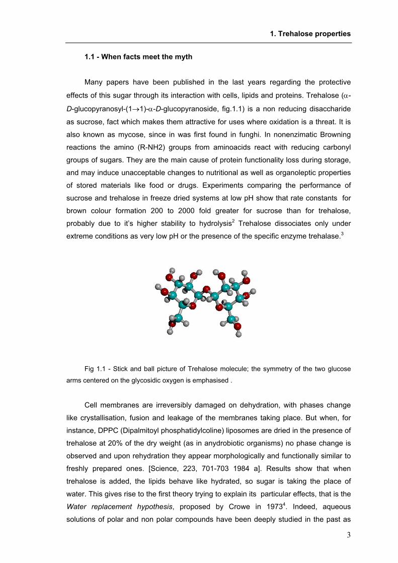
Fig 1.1 - Stick and ball picture of Trehalose molecule; the symmetry of the two glucose
arms centered on the glycosidic oxygen is emphasised .
Cell membranes are irreversibly damaged on dehydration, with phases change
like crystallisation, fusion and leakage of the membranes taking place. But when, for
instance, DPPC (Dipalmitoyl phosphatidylcoline) liposomes are dried in the presence of
trehalose at 20% of the dry weight (as in anydrobiotic organisms) no phase change is
observed and upon rehydration they appear morphologically and functionally similar to
freshly prepared ones. [Science, 223, 701-703 1984 a]. Results show that when
trehalose is added, the lipids behave like hydrated, so sugar is taking the place of
water. This gives rise to the first theory trying to explain its particular effects, that is the
Water replacement hypothesis, proposed by Crowe in 19734. Indeed, aqueous
solutions of polar and non polar compounds have been deeply studied in the past as
1. Trehalose properties
4
model systems for interpreting and predicting the behaviour of functional biological
macromolecules. The interplay of solute-solute and solute-solvent interactions has
been disclosed and sometimes arbitrarily catalogued (see, for example, papers and
references therein in the volume of Biophysical Chemistry 2003 dedicated to Walter
Kauzmann), nonetheless the stabilization of membranes by several solutes is complex
and not assignable to a specific contribution alone.
Yeasts accumulate trehalose in response to stresses. During fermentation, when
ethanol concentration rises, it starts poisoning cells triggering a natural signal for the
them to stop its production. Growth is inhibited, and cell metabolism decreases, so
does nutrient intake and ethanol production. Trehalose is likely to improve ethanol
tolerance by protecting the plasma membrane from leakage.5 Temperature is another
stress to consider on fermentation processes. For example when temperature changes
from 25°C to 40°C, trehalose is synthesized by cells along with heat shock proteins to
enhance their thermotollerance. Proteins would play a key role in the recovery from the
heat-stressed state whereas trehalose should be involved mainly in the protection of
proteins and enzimes from denaturation as discused below.3
Some proteins do not get damaged at all when freeze dried, but more labile ones
suffer degradation and denature, losing the possibility to come back to their original
conformation and as a consequence, losing functionality. Trehalose has proven to
protect this kind of proteins, and some significant results attribute an efficiency of
almost 90%. Apparently, the extreme flexibility around the glycoside bond, conferred by
the lack of intramolecular hydrogen bonding, allows it to adapt to the irregular form of
proteins and bond to them. It can form up to four hydrogen bonds per molecule of
trehalose. In the stable dihydrate molecule of trehalose, these bonds are formed with
water. Nevertheless, IR and Raman experiments studying the interaction between
trehalose and the protein lysozyme suggest that rather than binding to it, trehalose
keeps the remaining water near the protein avoiding complete dehydration.6 Moreover,
there was also the belief that as trehalose would have a considerably large hydrated
radius, it would be excluded from the hydration shell of proteins. According to Sola-
Penna and coworkers, hydrated trehalose occupies 2.5 fold larger volume than
sucrose, maltose, glucose and fructose.7 As a consequence, this preferential exclusion
mechanism would be responsible of the preservation.8 However, an analysis of the
actual experimental viscosity data reported in the paper show that some unclear
mistakes occurred in their elaboration, since their results do not agree with most of
what reported in literature, nor with the experimental data repeated in our laboratory
and reported in another Ph.D. Thesis (F. Sussich, Trieste 2004). In our opinion, both
the wrong conclusions of Sola Penna and the reporting of a visual perception (sic!) of
1. Trehalose properties
5
the larger hydration volume induced other researchers to consider this phenomenon
highly relevant. Indeed, even if the high viscosity attributed to trehalose is not such, as
other measurements show, perhaps this mistake made years ago induced also
Magazù9 to emphasize that trehalose has a bigger hydration ratio than its isomers
sucrose and maltose. Although their calculations are based on a series of
approximations, the difference between sugar volumes is not as drastic as that
reported by Sola Penna. Although the hydrogen bonding protection mechanism can
partially explain the efficiency of trehalose, other mono or disaccharides should act as
well as it, if this was the only cause. Nevertheless, glucose is not that effective, mostly
when considering freeze-drying. It was shown that besides the hydrogen bonding
capability, a good cryoprotectant should be able to conserve the native structure of the
protein in the dry state. Protein conformation is known to be severely conditioned by
the matrix that surrounds it. At this point, another property of trehalose comes to light,
it’s high glass transition temperature. Comparing to the other disaccharides, trehalose
has an exceptionally high glass transition temperature, implying that at drying
conditions it is already a glass. Proteins are immobilised in this viscous glassy matrix
and therefore they cannot denature. Green and Angell mentioned this feature which
constitutes another theory trying to explain the mechanisms behind trehalose
bioprotective action, the glass hypothesis. In their paper10, the comparison of the glass
transition temperatures of trehalose and glucose was made and a Tg = 79 °C was
reported for trehalose, that is higher than sucrose and other disaccharides (Note that
the true Tg of trehalose is as high as 120 °C, nonetheless this work is continuously
quoted for the very high Tg of trehalose; the concept is correct, but the number is
wrong). Anyway, they highlight this elevated glass transition temperature (Tg), which
became to be known as the trehalose anomaly. Experiments were conducted onto
elucidating this issue but even when many features of the glass and solution states are
known there are no satisfactory explanations to it. Part of this PhD thesis deals with it
and the results obtained will be exposed and analysed in the frame of these and other
hypothesis.
All the properties mentioned above make trehalose very attractive for a wide
range of applications, going from the biomedical to the food or cosmetic science ( see
references 11-13 and references therein). It is used in different areas as moisturizer,
preserving agent, sweetener and for the stabilization of liposomes in cosmetics. 14 It
could have an invaluable contribution in stabilising vaccines, immunoconjugates,
antisera ecc. during storage at room temperature or even higher, overcoming problems
arising from a break in the cold chain and decreasing dramatically the cost of
distribution, making them accessible for everyone. After several successful
1. Trehalose properties
6
experiences in freeze-drying of human platelets, mammalian cells, etc the most
ambitious are already talking about stabilisation of organs for transplantations and
Langherans islet transplants 15-22
So it comes out straightforward that understanding the mechanisms underlying
bioprotection would have remarkable implications in the progress of science and
technology.
1.2 - Bioprotection: how does it work? The water replacement, preferential exclusion and glass hypothesis were already
mentioned as they were initially found in literature as the answer to the question of
bioprotection. In the last years, other hypothesis arose as the formers where not
satisfying. The destructuring effect mechanism states that trehalose imposes a
determined spatial location to the water molecules surrounding it, an effect that was
verified with molecular dynamic simulations. According to these simulations23,24 it
conditions the structure of water up to the third hydration shell. Doing so, tetrahedral
coordination is banned and water is unable to nucleate and crystallise, so the damages
produced by the formation of ice do not take place. Many authors believe that this
destructuring effect is possible because trehalose-solvent/solute interactions are
favoured above solvent-solvent ones.9 Water would bind stronger to trehalose than to
other water molecules in what they call “preferential interaction”. It is interesting to
reflect about the implications of these preferential interactions on proteins; several
papers show these interactions occur, contradicting the preferential exclusion
mechanism.
An appealing hypothesis involves the possibility that some crystalline forms
(dihydrate and anhydrous crystals) could be also implied in bioprotection. It was
observed that when dried membranes where rehydrated with water vapour, the
dihydrate crystal was formed.13 The crystal “traps” two water molecules per sugar, so
that part of glassy trehalose converts into its dihydrate minimizing the free water
content. In this way, the rest of the matrix remains as a glass, as there’s no water
plasticizing it.25 This hypothesis was supported by some additional experimental
evidences and it is becoming more and more clear since the conversion between the
dihydrate crystalline and the anhydrous crystalline phase, obtained under certain
particular conditions, is fully reversible.26 In this view, a synergic effect toward the
immobilisation of a biomolecule should be ascribed to the formation of the anhydrous
crystalline/amorphous mixture, starting from the removal of water from the aqueous
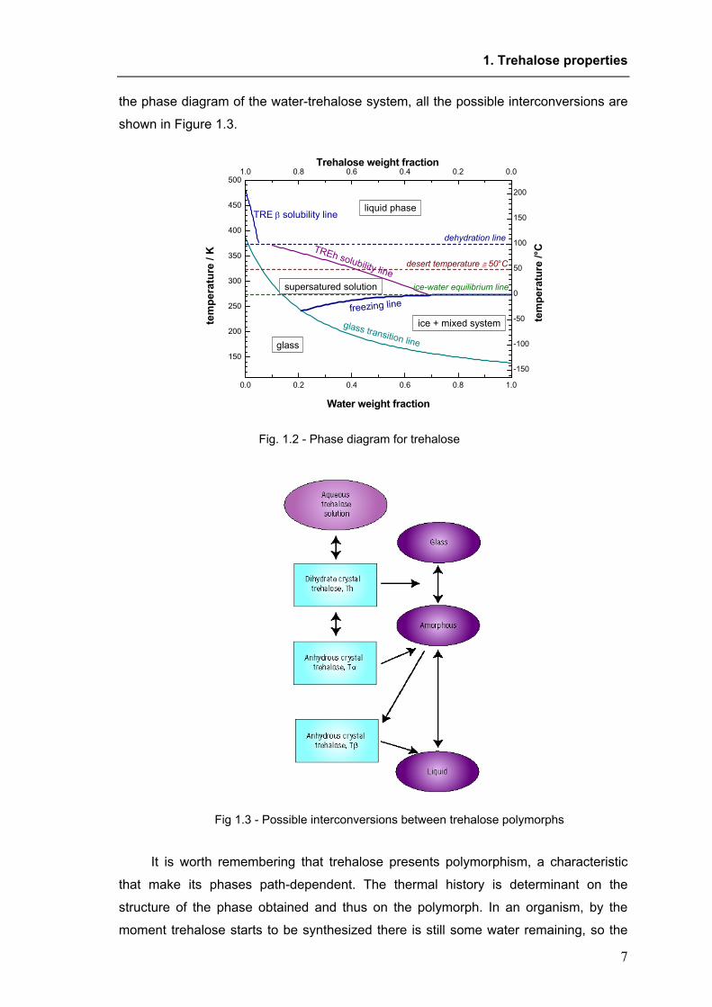
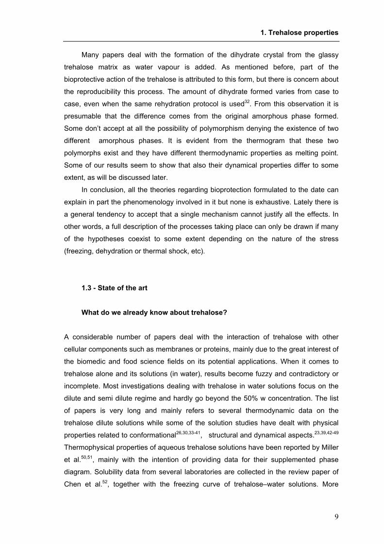
solution of concentrated trehalose (see the phase diagram in Figure 1.2). In addition to
1. Trehalose properties
7
1.0 0.8 0.6 0.4 0.2 0.0
-150
-100
-50
0
50
100
150
200
0.0 0.2 0.4 0.6 0.8 1.0
150
200
250
300
350
400
450
500
dehydration line
ice-water equilibrium line
desert temperature ≅ 50°C
TRE β solubility line
tem
pera
ture
/°C
Trehalose weight fraction
glass transition line
TREh solubility line
freezing line
glass
ice + mixed system
supersatured solution
liquid phase
tem
pera
ture
/ K
Water weight fraction
the phase diagram of the water-trehalose system, all the possible interconversions are
shown in Figure 1.3.
Fig. 1.2 - Phase diagram for trehalose
Fig 1.3 - Possible interconversions between trehalose polymorphs
It is worth remembering that trehalose presents polymorphism, a characteristic
that make its phases path-dependent. The thermal history is determinant on the
structure of the phase obtained and thus on the polymorph. In an organism, by the
moment trehalose starts to be synthesized there is still some water remaining, so the

1. Trehalose properties
8
first species formed is the solution. The latter evolves into the dihydrate crystal as
water decreases and the concentration approaches two water molecules per sugar.
The three-dimensional sketch of the dihydrate crystal is represented in figure 1.4. The
crystal structure27,28 is made up by four sugar units C12H22O11·2H2O in an orthorhombic
cell (P212121). Water and trehalose molecules are held together in the crystal by a
complex system of twelve hydrogen bonds where every hydroxyl group of the trehalose
Fig. 1.4 Three-dimensional structure of the di-hydate crystal of trehalose
molecule is both donor and acceptor in the hydrogen bond net. However, in the crystal
there are no intramolecular hydrogen bonds such as in sucrose or cellobiose. 29
As dehydration proceeds, the dihydrate starts to lose water until when, under mild
conditions, becomes anhydrous. The anhydrous phase formed in this way, called
alpha-trehalose (TRE α) is not amorphous at all in our opinion, but formed by a series
of unstable, tiny crystals, as shown by its powder diffraction pattern.30 These crystals
can be in the order of a few nanometers and this is the reason why its structure hasn’t
been determined yet. Another temperature path, which implies the fast dehydration of
the dihydrate yields the beta-trehalose polymorph (TRE β), a very stable, fully
characterised crystal 31 with a high melting point, around 215 °C. TRE β cannot be
involved in the processes occurring in nature since its formation implies the presence
of environmental conditions and elevated temperatures which are not verified. Yet it is
surely involved in many industrial processes, then it deserves attention for
understanding trehalose transformations implies optimising results.
1. Trehalose properties
9
Many papers deal with the formation of the dihydrate crystal from the glassy
trehalose matrix as water vapour is added. As mentioned before, part of the
bioprotective action of the trehalose is attributed to this form, but there is concern about
the reproducibility this process. The amount of dihydrate formed varies from case to
case, even when the same rehydration protocol is used32. From this observation it is
presumable that the difference comes from the original amorphous phase formed.
Some don’t accept at all the possibility of polymorphism denying the existence of two
different amorphous phases. It is evident from the thermogram that these two
polymorphs exist and they have different thermodynamic properties as melting point.
Some of our results seem to show that also their dynamical properties differ to some
extent, as will be discussed later.
In conclusion, all the theories regarding bioprotection formulated to the date can
explain in part the phenomenology involved in it but none is exhaustive. Lately there is
a general tendency to accept that a single mechanism cannot justify all the effects. In
other words, a full description of the processes taking place can only be drawn if many
of the hypotheses coexist to some extent depending on the nature of the stress
(freezing, dehydration or thermal shock, etc).
1.3 - State of the art What do we already know about trehalose?
A considerable number of papers deal with the interaction of trehalose with other
cellular components such as membranes or proteins, mainly due to the great interest of
the biomedic and food science fields on its potential applications. When it comes to
trehalose alone and its solutions (in water), results become fuzzy and contradictory or
incomplete. Most investigations dealing with trehalose in water solutions focus on the
dilute and semi dilute regime and hardly go beyond the 50% w concentration. The list
of papers is very long and mainly refers to several thermodynamic data on the
trehalose dilute solutions while some of the solution studies have dealt with physical
properties related to conformational26,30,33-41, structural and dynamical aspects.23,39,42-49
Thermophysical properties of aqueous trehalose solutions have been reported by Miller
et al.50,51, mainly with the intention of providing data for their supplemented phase
diagram. Solubility data from several laboratories are collected in the review paper of
Chen et al.52, together with the freezing curve of trehalose–water solutions. More

1. Trehalose properties
10
recently, a particular attention has been given to trehalose in confined state, where
experimentals and MD simulations would be of interest also for the in vivo situation.
On the other hand, many studies have dealt with the thermodynamic, structural
and dynamical properties of the anhydrous undercooled liquid of trehalose, mainly to
characterise the glass transition region. Here, additional quotation is made to the
molecular mobility of undercooled liquid trehalose studied by temperature-modulated
differential scanning calorimetry and by dielectric analysis53 and to the work carried out
by Lefort et al54,55. The greater molecular mobility of trehalose glass with respect to
other sugars, such as lactose and sucrose, has been inferred in this latter recent study
by Lefort et al. on the basis of solid state NMR and computational investigation on
sugar glasses.
The larger internal mobility of trehalose is however accompanied by the ability of
trehalose to form larger clusters than sucrose.56 Subsequently, on the basis of the
enthalpy relaxation studies of the three sugars, lactose, sucrose and trehalose, during
isothermal aging, it has been shown that the size of the cooperative regions in the
temperature range between 298 and 365 K is much larger for trehalose than for
sucrose and lactose57. They all provide some hints in the actual mobility of trehalose
molecules in the amorphous/glassy state.
Quasi elastic and inelastic neutron scattering, neutron spin echo Affouard et al.58
studied the effect of sugar on water by means of QENS and INS, comparing trehalose
and sucrose at 50% w concentration. Their findings suggest that the addition of
trehalose and sucrose to water slow down considerably the dynamics of water. NSE
experiments evidence the kosmotropic character of these sugars. This kind of
molecules impose their own order to water, preventing the formation of the tetrahedral
hydrogen bonded network of water, thus hindering ice crystallisation. In agreement with
NSE, INS results demonstrate how water translational diffusion is slowed down in the
presence of disaccharides and how this effect is more pronounced for trehalose. By
their estimation, the dynamics of a 49%w solution of sugar at T=320 K resembles that
of pure water at temperatures around 268K in the case of trehalose and 277 K for
sucrose solutions. According to this, adding 50% w trehalose to water would have on
its dynamics the effect of cooling down to -5°C (freezing). A comparison among
trehalose, sucrose and maltose shows that the former has a higher “crystalline-like”
behaviour in solution, a higher degree of local order, forming a single entity with water,
what would justify its rigidity comparing to other disaccharide solutions.
Therefore, some effects of the sugar trehalose on the water properties seem to
be distinctive with respect to other sugars. How these effects converge to the
1. Trehalose properties
11
bioprotectant action of trehalose when water molecules are absent or very rare is not
clear yet.
As a further comment, from the literature analysis a gap of information appears
on concentrated solutions. Dilute solutions can give useful information about the
dynamics of water in the presence of sugar. It is obviously the starting point, and some
differences between isomers can already be evident in these range of concentrations.
From the commercial point of view, applications dealing with freeze drying and the
preservation of solutions, mainly at low temperatures, have certainly taken advantage
of these findings. Nevertheless, glass formation in environmental conditions involves
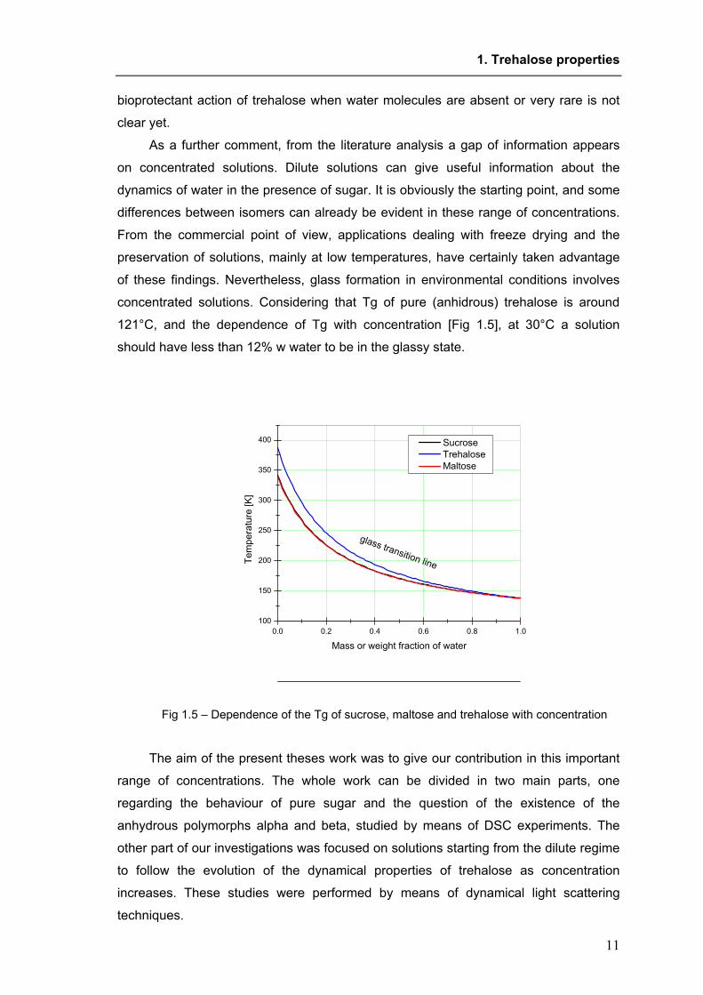
concentrated solutions. Considering that Tg of pure (anhidrous) trehalose is around
121°C, and the dependence of Tg with concentration [Fig 1.5], at 30°C a solution
should have less than 12% w water to be in the glassy state.
0.0 0.2 0.4 0.6 0.8 1.0100
150
200
250
300
350
400
glass transition lineTem
pera
ture
[K]
Mass or weight fraction of water
Sucrose Trehalose Maltose
Fig 1.5 – Dependence of the Tg of sucrose, maltose and trehalose with concentration
The aim of the present theses work was to give our contribution in this important
range of concentrations. The whole work can be divided in two main parts, one
regarding the behaviour of pure sugar and the question of the existence of the
anhydrous polymorphs alpha and beta, studied by means of DSC experiments. The
other part of our investigations was focused on solutions starting from the dilute regime
to follow the evolution of the dynamical properties of trehalose as concentration
increases. These studies were performed by means of dynamical light scattering
techniques.
References for Introduction and Chapter 1
12
References
1. Keilin, D. Proceedings of the Royal Society of London. Series B, Biological
Sciences., pp. 149-191 London,1959).
2. O'BRIEN, J. Stability of Trehalose, Sucrose and Glucose to Nonenzymatic Browning in Model Systems. Journal of Food Science 61, 679-682 (1996).
3. Paiva, C. L. & Panek, A. D. Biotechnological applications of the disaccharide trehalose 1. Biotechnol. Annu. Rev. 2, 293-314 (1996).
4. CROWE, J. H., CROWE, L. M. & CHAPMAN, D. Preservation of Membranes in Anhydrobiotic Organisms: The Role of Trehalose. Science 223, 701-703 (1984).
5. Crowe, J. H. a. J. S. C. Anhydrobiosis. Hutchinson & Ross, Stroundsburg, (1973).
6. Mansure, J. J. C., Panek, A. D., CROWE, L. M. & CROWE, J. H. Trehalose inhibits ethanol effects on intact yeast cells and liposomes. Biochimica et Biophysica Acta (BBA) - Biomembranes 1191, 309-316 (1994).
7. Belton, P. S. & Gil, A. M. IR and Raman spectroscopic studies of the interaction of trehalose with hen egg white lysozyme. Biopolymers 34, 957-961 (1994).
8. Sola-Penna, M. & Meyer-Fernandes, J. R. Stabilization against Thermal Inactivation Promoted by Sugars on Enzyme Structure and Function: Why Is Trehalose More Effective Than Other Sugars? Archives of Biochemistry and Biophysics 360, 10-14 (1998).
9. Xie, G. & Timasheff, S. N. The thermodynamic mechanism of protein stabilization by trehalose. Biophysical Chemistry10 Years of the Gibbs Conference on Biothermodynamics 64, 25-43 (1997).
10. Sussich, F. PhD. Thesis. 2004. University of Trieste. Ref Type: Thesis/Dissertation
11. Branca, C. et al. Tetrahedral order in homologous disaccharide-water mixtures 2. J. Chem. Phys. 122, 174513 (2005).
12. Green, J. L. & Angell, C. A. Phase relations and vitrification in saccharide-water solutions and the trehalose anomaly. Journal of Physical Chemistry 93, 2880-2882 (1989).
13. Crowe, J. H. et al. The trehalose myth revisited: Introduction to a symposium on stabilization of cells in the dry state. Cryobiology 43, 89-105 (2002).
14. Crowe, J. H. Trehalose as a "chemical chaperone": fact and fantasy. Advances in experimental medicine and biology 594, 143-158 (2007).
15. Crowe, L. M., Reid, D. S. & Crowe, J. H. Is trehalose special for preserving dry biomaterials? Biophys. J. 71, 2087-2093 (1996).
16. Schiraldi, C., Di Lernia, I. & De Rosa, M. Trehalose production: exploiting novel approaches. Trends in Biotechnology 20, 420-425 (2002).

References for Introduction and Chapter 1
13
17. Crowe, J. H. et al. The trehalose myth revisited: introduction to a symposium on stabilization of cells in the dry state. Cryobiology 43, 89-105 (2001).
18. Crowe, J. H. & Crowe, L. M. Preservation of mammalian cells-learning nature's tricks. Nat. Biotechnol. 18, 145-146 (2000).
19. Crowe, L. M., Reid, D. S. & Crowe, J. H. Is trehalose special for preserving dry biomaterials? Biophys. J. 71, 2087-2093 (1996).
20. Beattie, G. M. et al. Trehalose: a cryoprotectant that enhances recovery and preserves function of human pancreatic islets after long-term storage 14. Diabetes 46, 519-523 (1997).
21. Chen, F., Nakamura, T. & Wada, H. Development of new organ preservation solutions in Kyoto University 6. Yonsei Med. J. 45, 1107-1114 (2004).
22. Katenz, E. et al. Cryopreservation of primary human hepatocytes: the benefit of trehalose as an additional cryoprotective agent 3. Liver Transpl. 13, 38-45 (2007).
23. Scheinkonig, C., Kappicht, S., Kolb, H. J. & Schleuning, M. Adoption of long-term cultures to evaluate the cryoprotective potential of trehalose for freezing hematopoietic stem cells 8. Bone Marrow Transplant. 34, 531-536 (2004).
24. Tang, M., Wolkers, W. F., Crowe, J. H. & Tablin, F. Freeze-dried rehydrated human blood platelets regulate intracellular pH. Transfusion 46, 1029-1037 (2006).
25. Engelsen, S. B. & Ferez, S. Unique similarity of the asymmetric trehalose solid-state hydration and the diluted aqueous-solution hydration. Journal of Physical Chemistry B 104, 9301-9311 (2000).
26. Lerbret, A. et al. Influence of homologous disaccharides on the hydrogen-bond network of water: Complementary Raman scattering experiments and molecular dynamics simulations. Carbohydrate Research 340, 881-887 (2005).
27. Branca, C. et al. Tetrahedral order in homologous disaccharide-water mixtures 2. J. Chem. Phys. 122, 174513 (2005).
28. Horvat, M., Mestrovic, E., Danilovski, A. & Craig, D. Q. M. An investigation into the thermal behaviour of a model drug mixture with amorphous trehalose. International Journal of Pharmaceutics 294, 1-10 (2005).
29. Sussich, F. & Cesàro, A. Transitions and phenomenology of a,a-trehalose polymorphs inter-conversion. Journal of Thermal Analysis and Calorimetry 62, 757-768 (2000).
30. Brown, G. M. et al. The crystal structure of alpha,alpha-trehalose dihydrate from three independent X-ray determinations. Acta Crystallographica Section B 28, 3145-3158 (1972).
31. Taga, T., Senma, M. & Osaki, K. The crystal and molecular structure of trehalose dihydrate. Acta Crystallographica Section B 28, 3258-3263 (1972).

References for Introduction and Chapter 1
14
32. Cesàro, A., De Giacomo, O. & Sussich, F. Water interplay in trehalose polymorphism. Food Chemistry4th International Workshop on Water in Foods 106, 1318-1328 (2008).
33. Sussich, F., Urbani, R., Princivalle, F. & Cesàro, A. Polymorphic amorphous and crystalline forms of trehalose. Journal of the American Chemical Society 120, 7893-7899 (1998).
34. Jeffrey, G. A. & Nanni, R. The crystal structure of anhydrous alpha,alpha-trehalose at -150 degrees 1. Carbohydr. Res. 137, 21-30 (1985).
35. Akao, K., Okubo, Y., Asakawa, N., Inoue, Y. & Sakurai, M. Infrared spectroscopic study on the properties of the anhydrous form II of trehalose. Implications for the functional mechanism of trehalose as a biostabilizer. Carbohydrate Research 334, 233-241 (2001).
36. Abbate, S., Conti, G. & Naggi, A. Characterisation of the glycosidic linkage by infrared and Raman spectroscopy in the C-H stretching region: a,a-trehalose and a,a-trehalose-2,3,4,6,6-d10. Carbohydr. Res. 210, 1-12 (1991).
37. Batta, G., Kover, K. E., Gervay, J., Hornyak, M. & Roberts, G. M. Temperature dependence of molecular conformation, dynamics, and chemical shift anisotropy of a,a-trehalose in D2O by NMR relaxation. Journal of the American Chemical Society 119, 1336-1345 (1997).
38. Batta, G. & Kover, K. E. Heteronuclear coupling constants of hydroxyl protons in a water solution of oligosaccharides: Trehalose and sucrose. Carbohydrate Research 320, 267-272 (1999).
39. Bonanno, G., Noto, R. & Fornili, S. L. Water interaction with ?,?-trehalose: Molecular dynamics simulation. Journal of the Chemical Society - Faraday Transactions 2755-2762 (1998).
40. Conrad, P. B. & De Pablo, J. J. Computer simulation of the cryoprotectant disaccharide a,a-trehalose in aqueous solution. Journal of Physical Chemistry A 103, 4049-4055 (1999).
41. Liu, Q., Schmidt, R. K., Teo, B., Karplus, P. A. & Brady, J. W. Molecular dynamics studies of the hydration of a,a-trehalose. Journal of the American Chemical Society 119, 7851-7862 (1997).
42. Sakurai, M., Murata, M., Inoue, Y., Hino, A. & Kobayashi, S. Molecular-dynamics study of aqueous solution of trehalose and maltose: Implication for the biological function of trehalose 18. Bulletin of the Chemical Society of Japan 70, 847-858 (1997).
43. Sussich, F., Princivalle, F. & Cesàro, A. The interplay of the rate of water removal in the dehydration of a,a-trehalose. Carbohydrate Research 322, 113-119 (1999).
44. Westh, P. & Raml°v, H. Trehalose accumulation in the tardigrade Adorybiotus coronifer during anhydrobiosis 124. J. Exp. Zool. 258, 303-311 (1991).
References for Introduction and Chapter 1
15
45. Branca, C. et al. The fragile character and structure-breaker role of :á, á-trehalose: Viscosity and Raman scattering findings 21. Journal of Physics Condensed Matter 11, 3823-3832 (1999).
46. Branca, C., Magazù, S., Maisano, G. & Migliardo, P. a,a-trehalose-water solutions. 3. Vibrational dynamics studies by inelastic light scattering 22. Journal of Physical Chemistry B 103, 1347-1353 (1999).
47. Dowd, M. K., Reilly, P. J. & French, A. D. Conformational analysis of trehalose disaccharides and analogues using MM3. J. Comput. Chem. 13, 102-114 (1992).
48. Duda, C. A. & Stevens, E. S. Trehalose Conformation in Aqueous Solution from Optical Rotation 17. J. Am. Chem. Soc. 112, 7406-7407 (1990).
49. Elias, M. E. & Elias, A. M. Trehalose + water fragile system: Properties and glass transition. Journal of Molecular Liquids 83, 303-310 (1999).
50. Galema, S. A. & Hoiland, H. Stereochemical aspects of hydration of carbohydrates in aqueous solutions. 3. Density and ultrasound measurements 24. Journal of Physical Chemistry 95, 5321-5326 (1991).
51. Karger, N. & demann, H. D. Temperature dependence of the rotational mobility of the sugar and water molecules in concentrated aqueous trehalose and sucrose solutions 25. Zeitschrift fur Naturforschung. C, Journal of biosciences 46, 313-317 (1991).
52. Librizzi, F., Vitrano, E. & Cordone, L. Dehydration and crystallization of trehalose and sucrose glasses containing carbonmonoxy-myoglobin 26. Biophysical Journal 76, 2727-2734 (1999).
53. Miller, D. P., De Pablo, J. J. & Corti, H. Thermophysical Properties of Trehalose and Its Concentrated Aqueous Solutions 28. Pharmaceutical Research 14, 578-590 (1997).
54. Miller, D. P., De Pablo, J. J. & Corti, H. R. Viscosity and glass transition temperature of aqueous mixtures of trehalose with borax and sodium chloride 27. Journal of Physical Chemistry B 103, 10243-10249 (1999).
55. Chen, T., Fowler, A. & Toner, M. Literature review: Supplemented phase diagram of the trehalose-water binary mixture. Cryobiology 40, 277-282 (2000).
56. De Gusseme, A., Carpentier, L., Willart, J. F. & Descamps, M. Molecular mobility in supercooled trehalose. Journal of Physical Chemistry B 107, 10879-10886 (2003).
57. Lefort, R., Bordat, P., Cesàro, A. & Descamps, M. Exploring the conformational energy landscape of glassy disaccharides by cross polarization magic angle spinning C13 nuclear magnetic resonance and numerical simulations. II. Enhanced molecular flexibility in amorphous trehalose 31. Journal of Chemical Physics 126, (2007).
58. Lefort, R., Bordat, P., Cesàro, A. & Descamps, M. Exploring conformational energy landscape of glassy disaccharides by cross polarization magic angle spinning 13C NMR and numerical simulations. I. Methodological aspects 32. The Journal of Chemical Physics 126, 014510 (2007).

References for Introduction and Chapter 1
16
59. Lerbret, A., Bordat, P., Affouard, F., Descamps, M. & Migliardo, F. How homogeneous are the trehalose, maltose, and sucrose water solutions? An insight from molecular dynamics simulations. Journal of Physical Chemistry B 109, 11046-11057 (2005).
60. Haque, M. K., Kawai, K. & Suzuki, T. Glass transition and enthalpy relaxation of amorphous lactose glass 1. Carbohydr. Res. 341, 1884-1889 (2006).
61. Affouard, F. et al. A combined neutron scattering and simulation study on bioprotectant systems. Chemical Physics 317, 258-266 (2005).
2. The glassy state
17
2.1 - What is a glass?
So far the glassy state has been mentioned several times as responsible of many
of the exceptional properties of trehalose, but what is a glass?.
Angell1 gave the following definition: “A glass is a condensed state of matter
which has become non-ergodic by virtue of the continuous slow down for one or more
of its degrees of freedom”. On this approach matter is seen having a degree of freedom
that fluctuates at a rate strongly dependent on temperature and pressure and become
so slow for low T or high P that fluctuations are frozen. A phenomenological description
of this state follows.
A straightforward way to obtain a glass is heating a solid (for example, a
crystalline material) above its melting point, then taking energy away from it fast
enough to reach what is called the undercooled liquid state. When going through the
crystallisation temperature, this liquid will either crystallise or face the path leading into
the glassy state, depending on its intrinsic chemical structure and on operative
parameters such as the cooling rate. From the theoretical point of view any liquid,
cooled with a proper rate under its crystallisation point, should become a glass,
although experimentally cooling rates are finite so there is a limit in the possibility to
prove if this affirmation is true for every system. Substances capable of forming glasses
with the experimentally available cooling rates are generally referred as “glass
formers”, in particular “good glass formers” if the cooling rate is slow.
In the glassy state, the material has many solid-like properties but its X-ray
diffraction pattern resembles qualitatively the one for a liquid. In the liquid, molecules
rotate, diffuse, etc. As energy taken away from the system (it is cooled), some motions
decay as their energy barrier becomes too high to overcome. If this process occurs
slowly molecules are able to explore the conformational space and minimise their free
energy. As a consequence, without the presence of other conditions (for example steric
hindrance) ordering takes place and crystallisation arises. The phenomenon involves a
large group of molecules in long range interactions, and is characterised by the
periodicity of distribution, homogeneity reflected in a diffraction pattern as a series of
Bragg peaks. Conversely, when cooling fast, motion is restricted and molecules are
quenched in a configuration away from equilibrium, most commonly in a local energy
minimum, preventing ordering. Thus, long range order is not possible and the material
formed in this way is not homogeneous. This amorphous solid phase is known as
glass.
2. The glassy state
18
2.2 - Stability of the glassy phase
The first conclusion arriving intuitively is the liquid to glass transition is not an
equilibrium process. The system quenched in a local energy minimum could, in
principle, evolve to a global minimum energy state. As there is a finite probability for
this process to occur, the system is considered metastable. According to the level of
probability, the amorphous phase can be classified as relatively stable or unstable .
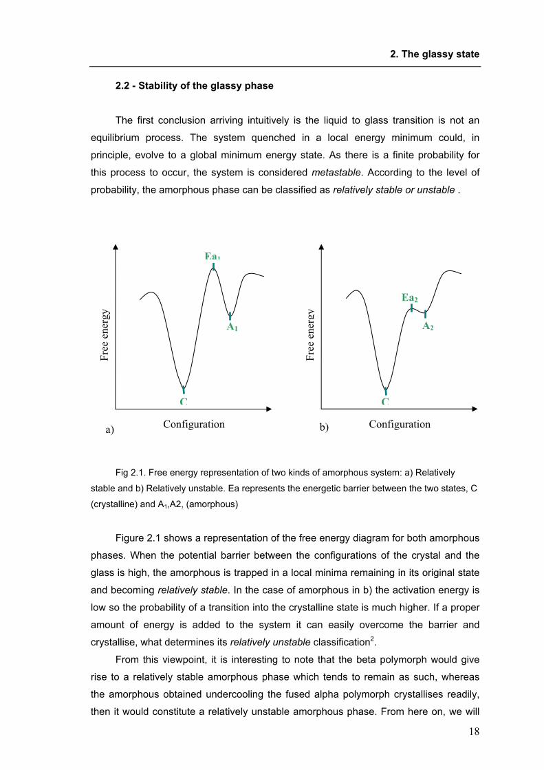
Fig 2.1. Free energy representation of two kinds of amorphous system: a) Relatively
stable and b) Relatively unstable. Ea represents the energetic barrier between the two states, C
(crystalline) and A1,A2, (amorphous)
Figure 2.1 shows a representation of the free energy diagram for both amorphous
phases. When the potential barrier between the configurations of the crystal and the
glass is high, the amorphous is trapped in a local minima remaining in its original state
and becoming relatively stable. In the case of amorphous in b) the activation energy is
low so the probability of a transition into the crystalline state is much higher. If a proper
amount of energy is added to the system it can easily overcome the barrier and
crystallise, what determines its relatively unstable classification2.
From this viewpoint, it is interesting to note that the beta polymorph would give
rise to a relatively stable amorphous phase which tends to remain as such, whereas
the amorphous obtained undercooling the fused alpha polymorph crystallises readily,
then it would constitute a relatively unstable amorphous phase. From here on, we will
A2
Ea2
C
Free
ene
rgy
Configuration
A1
C
Free
ene
rgy
Ea1
Configuration a) b)

2. The glassy state
19
call the amorphous phases obtained from the fusion of alpha and beta crystalline forms
as trehalose A and B, respectively. Figure 2.2 shows the different behaviour of A-
trehalose and B-trehalose phases on the same thermal cycle. The difference between
the amorphous phases could be relevant in the role of trehalose as a bioprotectant. We
propose that if this difference exists, it should be reflected on some property of the
glass and, chosen the right observable, experiments could demonstrate that the two
glasses obtained from alpha and beta behave in a different way under the same
environmental conditions. The search of this difference is one of the main motivations
of the calorimetric measurements performed.
Figure 2.2 – Thermal behaviour of the amorphous phases A trehalose and B trehalose.
It was previously said that the glass can be obtained cooling a liquid under its
melting point and that the state achieved is not in equilibrium, so a question emerges:
how to know when the phase transition takes place?
2.3 - The glass transition 2.3.1 – Thermodynamic considerations.
During a phase transition there is an evident change in the properties of matter. If
a determined property is monitored (e.g. enthalpy, entropy, specific heat, etc.) it is
A
B
2. The glassy state
20
possible to establish when the transition occurs. The glass transition is an exception in
this sense. Many properties show anomalies on their dependence on temperature
when approaching the Tg resembling a II order transition, although it is not the case.
(For a detailed treatment of this argument see ref [1] and references therein). Probably
the reason for this anomalies can be found in the departure from equilibrium, as it was
mentioned before, during the glass transition the thermic equilibrium of the liquid is lost.
This loss is sometimes called “ergodicity breaking” to emphasize the fact that glasses
are non-ergodic. On this scenario, a conventional definition of the glass transition is
needed.
One of the transport properties changing abruptly during the glass transition is the
viscosity. It depends strongly on temperature and can vary up to 14 orders of
magnitude when going through Tg. Experimentally it was observed that the viscosity of
many materials within this transformation range of temperatures was in the order of
1012 Pa.s, so it was adopted universally to define Tg as the temperature at which the
system reaches this viscosity value.
Another definition, regarding the thermodynamic aspects of the transition
describes it as the phenomenon where the derivatives of the amorphous phase
thermodynamic properties change more or less abruptly going from the values for the
liquid state to that of the crystal. The temperature at which a discontinuity is observed
is called the glass transition temperature Tg. However, some authors1 recalling the
kinetic character of this phenomenon prefer to talk about a glass transformation range
rather than temperature and underline the word transformation for what they hesitate to
call a transition.

2. The glassy state
21
Fig. 2.3 – Comparison between three different types of transition. a) Glass transiton; b)
second order transition; c) first order transition.
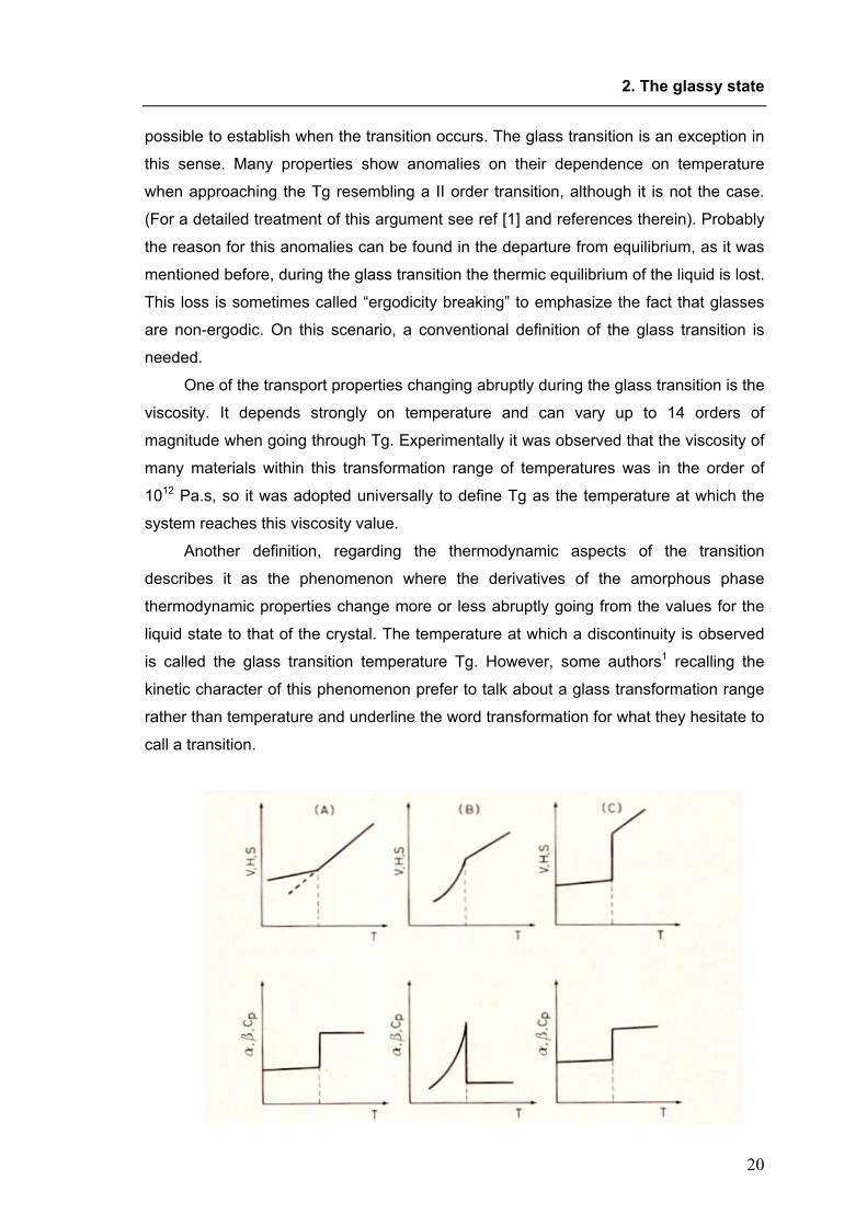
Figure 2.3 shows the temperature behaviour profile for enthalpy, entropy and
specific volume as an example for three different types of transition. A first order
transition (Fig. 6-c) presents a jump in the observed variables and also on the
derivatives, while a continuous change in variables (Fig6-a) characterises the glass
transition. This feature makes it similar to a II order transition (Fig.6-b).
The fact that a property change gradually makes it difficult to establish a unique
Tg. The most widely used technique to determine Tg is calorimetry. In a calorimetric
experiment, energy exchanged between the sample and the instrument is measured
against a reference as a function of time. The representation of that power versus
temperature is called a thermogram. If the system is in equilibrium at all times, the
magnitude represented corresponds to the heat capacity Cp. A typical thermogram
including the glass transition region is shown in 2.4.
Fig. 2.4 – Cp and enthalpy curves for a glass on heating (a) and cooling (b). Definition of
Tg onset, Tg midpoint.
There are several ways of determining Tg from a thermogram. The procedure
consists always in finding the cross point between the extrapolation of the properties of
the glass and the liquid. The most common one is Tg onset, which is the temperature
corresponding to the cross point between the extrapolations of the glass Cp and the
tangent at the inflection point of the sigmoidal baseline representing the glass
2. The glassy state
22
transition. Another used parameter is the Tg midpoint, which represents the point
where half of the mass has trespassed the glass transition. Tg Half-Width represents the
point on the curve that is halfway between the onset and end points. Still the Tg inflection
point is the point between the limits at which the slope of the curve changes from
increasing to decreasing or vice versa. The existence of different criteria for assigning
Tg explains is part the extensive range of temperatures attributed to the Tg of many
compounds, in our case trehalose.3,4 reported a Tg of 79°C; many authors agree that
Tg onset of trehalose is somewhere around 121°C. But there are other more relevant
factors conditioning the determination of Tg as will be discussed next.
2.3.2 – Kinetic considerations
It is clear at this point that the glass transition is a kinetically controlled
phenomenon. The characteristics of the glass are strongly conditioned by the methods
used to reach that state. Tg measured depends not only on the state of the glass
(thermal history, ageing etc) but also, and dramatically, on the scan rate. Generally
speaking, from this viewpoint the liquid has no “memory” and Tg determined during
cooling is more stable than Tg determined by heating. It was proposed that rather than
an arbitrary Tg with no physical meaning, a more representative parameter as Plazek’s
volume crossover or the Hodge cooling fictive temperature could be adopted.1
However, due to intrinsic instrumental problems, determining Tg on cooling may not be
the better choice in terms of precision, Another fact to consider is the entity of the
transition. For some materials, the Cp difference between the liquid and the glass may
be small, so the transition is difficult to detect.
Considering a Tg determined on heating, the higher the scan rate, the more will
the Tg be moving to higher temperatures, and viceversa for the cooling rate. It was
mentioned before that when the cooling rate is high, molecules have little time to
reorganise before the freezing of motion. It follows that a faster cooling will produce a
glass further from equilibrium than one obtained by slow cooling. Then, if the cooling
rate is very slow, the glass transition should be approximately similar to a real phase
transition. On this base, Anderson defined the ideal glass transition as the one
occurring over infinite times (rates near to 0), having the characteristics of a phase
transition.2
2. The glassy state
23
2.3.3 – The Kauzmann’s paradox
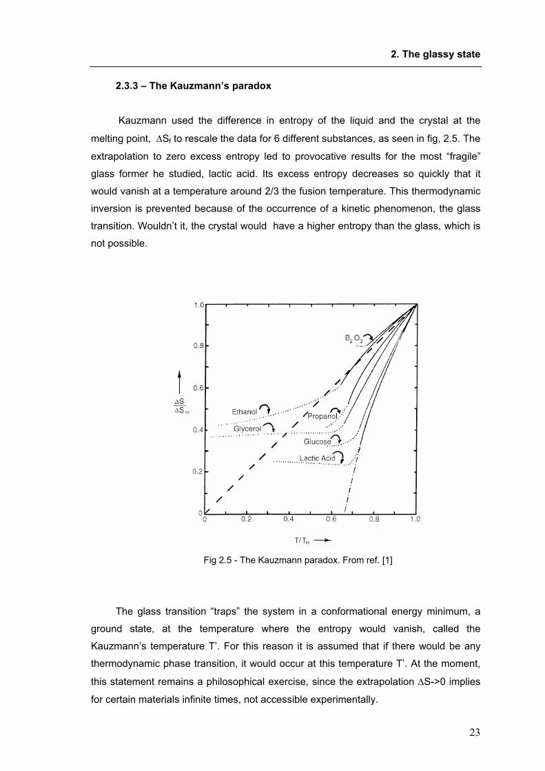
Kauzmann used the difference in entropy of the liquid and the crystal at the
melting point, ∆Sf to rescale the data for 6 different substances, as seen in fig, 2.5. The
extrapolation to zero excess entropy led to provocative results for the most “fragile”
glass former he studied, lactic acid. Its excess entropy decreases so quickly that it
would vanish at a temperature around 2/3 the fusion temperature. This thermodynamic
inversion is prevented because of the occurrence of a kinetic phenomenon, the glass
transition. Wouldn’t it, the crystal would have a higher entropy than the glass, which is
not possible.
Fig 2.5 - The Kauzmann paradox. From ref. [1]
The glass transition “traps” the system in a conformational energy minimum, a
ground state, at the temperature where the entropy would vanish, called the
Kauzmann’s temperature T’. For this reason it is assumed that if there would be any
thermodynamic phase transition, it would occur at this temperature T’. At the moment,
this statement remains a philosophical exercise, since the extrapolation ∆S->0 implies
for certain materials infinite times, not accessible experimentally.
2. The glassy state
24
2.3.4 Structural relaxation
At temperatures below but no so far from Tg, some diffusive motions are still
active in the glass. If a glass is let to “age” at this temperature for some time, molecules
reorganise in a tentative to minimise their energy and approach equilibrium. This
rearrangements are called structural relaxations and they are at the origin of what is
known as physical aging or annealing.
Goldstein and Gibbs5 established that the arrangement of molecules when a
liquid is cooled below Tg must be near the bottom of a potential energy minimum,
otherwise the glass would flow, which is known not to happen at temperatures below
half of the Tg. On the other hand, the existence of the ageing phenomenon on
temperatures near Tg implies that there are many minima which differ slightly in energy
one from another, also called “configurons”, that the particles explore until they arrive to
a sort of ground state. This state has an energy still well above that of the crystal and is
into it that the system tends to settle as excess entropy tends to vanish.
It is well known that ageing is strongly dependent on temperature. It is very fast
near the Tg and becomes slower as T decreases, mainly for two reasons. The first
regards the energy barrier between two minima, which gets harder to overcame as the
system looses energy. The second considers the entropic barriers raised as minima
become more distant. As a consequence, the rearranging group or the number of
successive rearrangements must be larger as temperature decreases.
The dependence of the viscosity with temperature in a simple liquid follows an
exponential behaviour, well represented by an Arrhenius like equation:
RTEaA +=ηln 2.1
This formula is also suitable for describing the viscosity dependence at T ≤Tg for
η intervals of 5 to 6 decades. Experimental data show a bending from this law at a
certain temperature, as if the activation energy would increase with decreasing
temperature. This was accounted for in the Vogel-Fulcher law:
))(exp( 00 TTTVFVFVF −= ηη 2.2

2. The glassy state
25
The VF law fits viscosity data for intervals of η changing 10 to 12 orders of
magnitude and anticipates a singularity at T=T0 forT0 located somewhere below Tg. A
fit of viscosity data with this two models is shown in figure 2.6 for comparison.
From this figure it is also comes out that there is a certain critical temperature
where the curve 1/η vs T changes trend, which implies also a change in the behaviour
of the structural relaxation. This temperature Tc, although not evident for some kind of
glass formers, has an important physical meaning, as the crossover temperature
between the dynamics of the liquid and the glass.
The most widely used expression to describe the evolution of the viscosity when
the Arrhenius behaviour fails is the Williams-Landel-Ferry equation, valid above Tg.
Applied to the viscosity it yields
)()(
loglog
2
1
g
g
Tg TTCTTC
−+
−−=
ηη
2.3
where ηTg is the viscosity at the Tg; C1 and C2 are fitting parameters, with values
around 17.4 and 51.6 respectively, changing slightly depending on the material. The
WLF semiempirical equation relates the viscosity of a liquid to a temperature scaled by
Tg therefore behaving as a universal law. However, Ferry and others expressed their
tri-α-naphtylbenzene
0.4 Ca(NO3)2 – 0.6 KNO3
Fig. 2.6 - Viscosity of CKN, Tg 333K, Tm 438K. fitted with an Arrhenius law: Log10η= -90 + 3430/T and TNB, Tg 69°C, Tm 199 °C fitted with a VF law, Log10h= -17.46 +4100/(T-200). Taken from ref. [6]

2. The glassy state
26
concerns about the interpretation of eq. 2.3 pointing out that it is somehow model
dependent as the value of the parameters C1 and C2 could change according to the
choice of Tg.
The characteristic time of molecular rearrangements τ is known to be in several
systems, according to a simple viscoelasticity model6 proportional to the viscosity by
the relation:
∞= G/ητ 2.4
Where ∞G is the high frequency limit of the shear modulus. By this relation it is
possible to observe that if the viscosity changes in 14 orders of magnitude through the
glass transition, the structural relaxation and as a consequence the characteristic
structural relaxation time τ also does. τ can be in the order of 10-12 s in the liquid state
to 100-102 s near the calorimetric glass transition when the dynamic of the system
slows down. In the approximation od weakly interacting spherical molecules, the
decrease in the translational diffusion can be described quantitatively, as it is also
proportional to the viscosity, by the Stokes-Einstein relation:
aTKD B
πη6= 2.5
Where D is the translational diffusion coefficient and a the effective radius of the
object diffusing, in this case the molecular diameter.
Analogously, the rotational diffusion is inversely proportional to the viscosity by
the Stokes-Einstein-Debye relation
3861
r
B
cr a
TKDπητ
=⟩⟨
≡ 2.6
where Dr is the rotational diffusion coefficient, ⟩⟨ cτ the mean rotational correlation
time and ar the spherical radius,
It is worth noting that although eq. 2.5 holds practically for all temperatures above
Tg, for many substances eq. 2.4 holds only for temperatures T>1.2 Tg 7. The latter was
verified for example, in a solution of sucrose in water, with fluorescein as tracer (similar
in size to sucrose8) , WLF and SE relations were combined with the same results,
supporting the supposition that around Tg diffusion would no longer be controlled by
the viscosity. Apparently, for temperatures below 1.2*Tg there is a pronounced
2. The glassy state
27
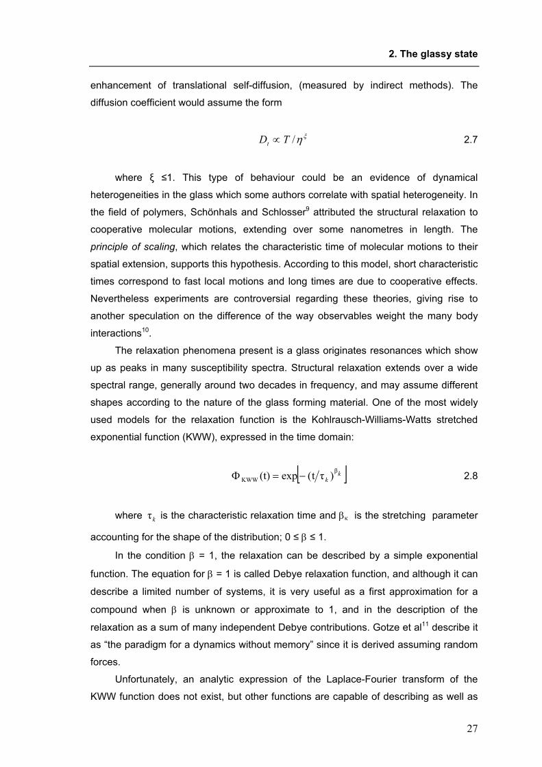
enhancement of translational self-diffusion, (measured by indirect methods). The
diffusion coefficient would assume the form
ξη/TDt ∝ 2.7
where ξ ≤1. This type of behaviour could be an evidence of dynamical
heterogeneities in the glass which some authors correlate with spatial heterogeneity. In
the field of polymers, Schönhals and Schlosser9 attributed the structural relaxation to
cooperative molecular motions, extending over some nanometres in length. The
principle of scaling, which relates the characteristic time of molecular motions to their
spatial extension, supports this hypothesis. According to this model, short characteristic
times correspond to fast local motions and long times are due to cooperative effects.
Nevertheless experiments are controversial regarding these theories, giving rise to
another speculation on the difference of the way observables weight the many body
interactions10.
The relaxation phenomena present is a glass originates resonances which show
up as peaks in many susceptibility spectra. Structural relaxation extends over a wide
spectral range, generally around two decades in frequency, and may assume different
shapes according to the nature of the glass forming material. One of the most widely
used models for the relaxation function is the Kohlrausch-Williams-Watts stretched
exponential function (KWW), expressed in the time domain:
[ ]kkβ
KWW )τt(exp(t) −=Φ 2.8
where kτ is the characteristic relaxation time and βκ is the stretching parameter
accounting for the shape of the distribution; 0 ≤ β ≤ 1.
In the condition β = 1, the relaxation can be described by a simple exponential
function. The equation for β = 1 is called Debye relaxation function, and although it can
describe a limited number of systems, it is very useful as a first approximation for a
compound when β is unknown or approximate to 1, and in the description of the
relaxation as a sum of many independent Debye contributions. Gotze et al11 describe it
as “the paradigm for a dynamics without memory” since it is derived assuming random
forces.
Unfortunately, an analytic expression of the Laplace-Fourier transform of the
KWW function does not exist, but other functions are capable of describing as well as
2. The glassy state
28
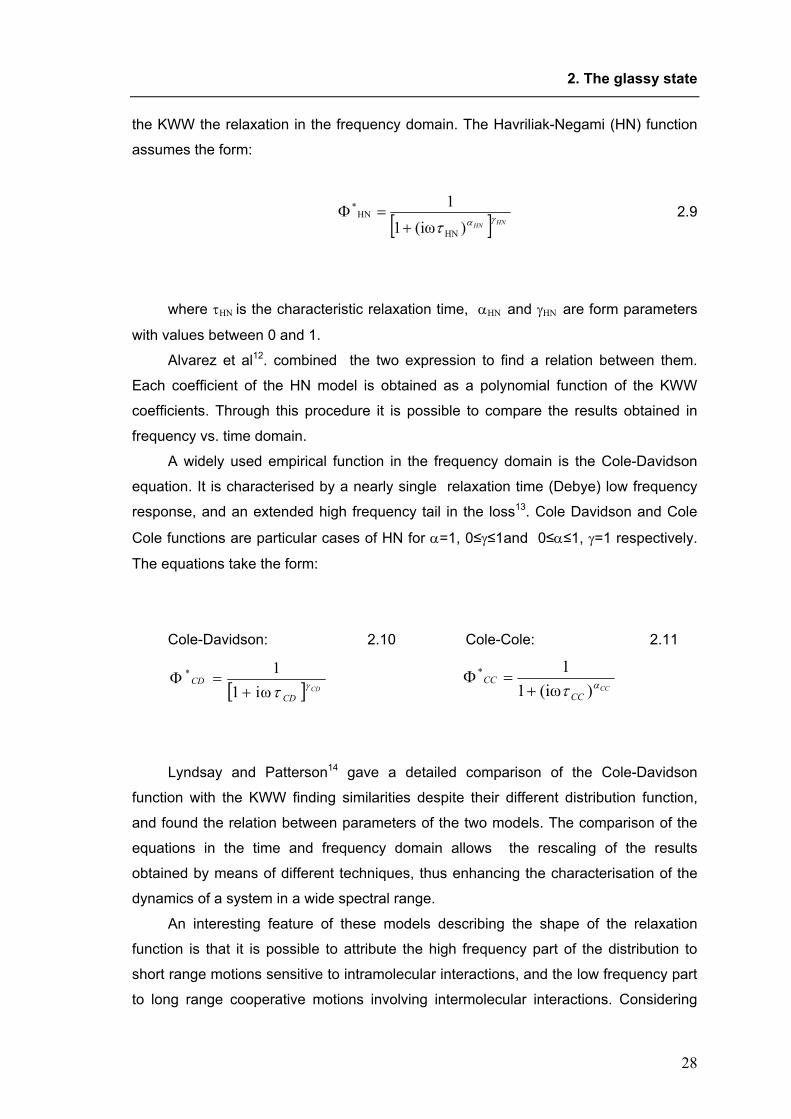
the KWW the relaxation in the frequency domain. The Havriliak-Negami (HN) function
assumes the form:
[ ] HNHNγατ )(iω1
1
HN
HN*
+=Φ 2.9
where τHN is the characteristic relaxation time, αHN and γHN are form parameters
with values between 0 and 1.
Alvarez et al12. combined the two expression to find a relation between them.
Each coefficient of the HN model is obtained as a polynomial function of the KWW
coefficients. Through this procedure it is possible to compare the results obtained in
frequency vs. time domain.
A widely used empirical function in the frequency domain is the Cole-Davidson
equation. It is characterised by a nearly single relaxation time (Debye) low frequency
response, and an extended high frequency tail in the loss13. Cole Davidson and Cole
Cole functions are particular cases of HN for α=1, 0≤γ≤1and 0≤α≤1, γ=1 respectively.
The equations take the form:
Cole-Davidson: 2.10 Cole-Cole: 2.11
[ ] CDCD
CD γτiω11*
+=Φ
CCCC
CC ατ )(iω11*
+=Φ
Lyndsay and Patterson14 gave a detailed comparison of the Cole-Davidson
function with the KWW finding similarities despite their different distribution function,
and found the relation between parameters of the two models. The comparison of the
equations in the time and frequency domain allows the rescaling of the results
obtained by means of different techniques, thus enhancing the characterisation of the
dynamics of a system in a wide spectral range.
An interesting feature of these models describing the shape of the relaxation
function is that it is possible to attribute the high frequency part of the distribution to
short range motions sensitive to intramolecular interactions, and the low frequency part
to long range cooperative motions involving intermolecular interactions. Considering
2. The glassy state
29
these dynamical aspects, Schonhals and Schlosser9 predict two different limit
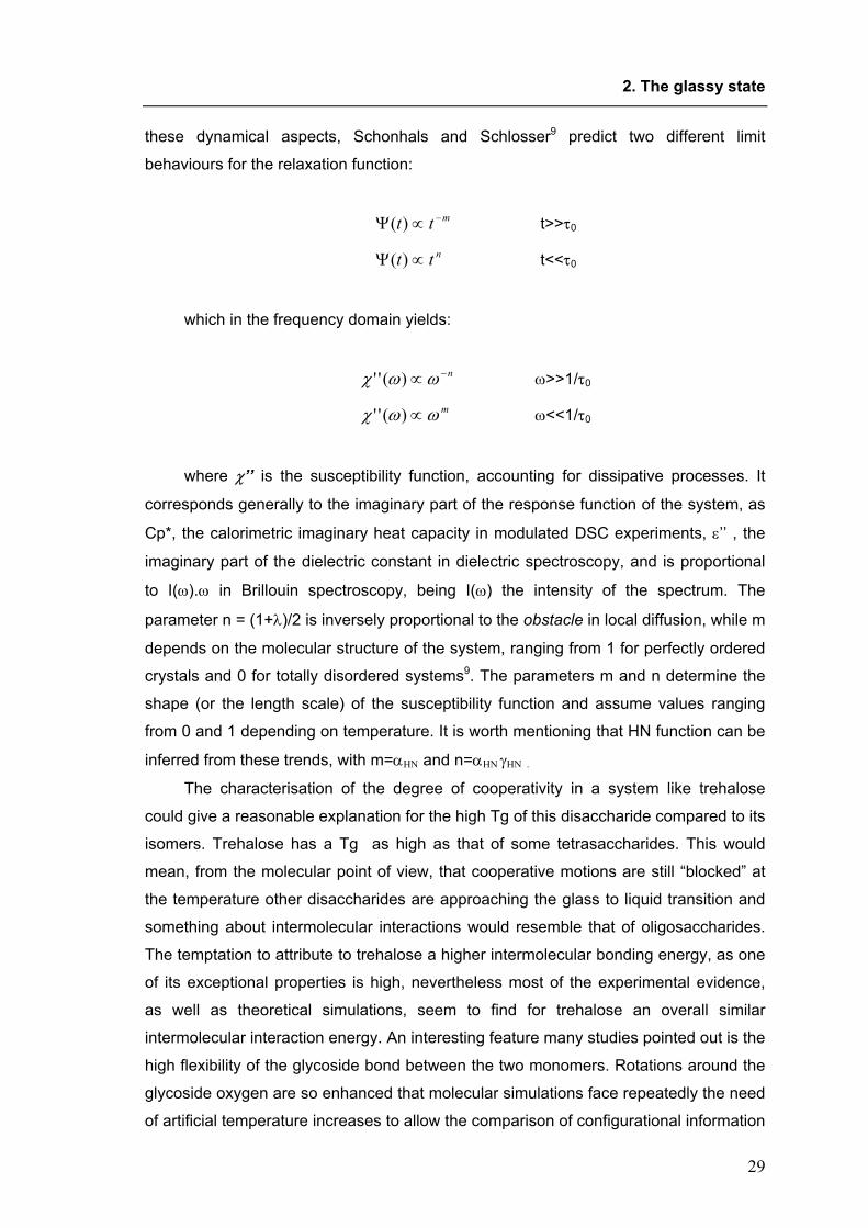
behaviours for the relaxation function:
mtt −∝Ψ )( t>>τ0
ntt ∝Ψ )( t<<τ0
which in the frequency domain yields:
n−∝ ωωχ )('' ω>>1/τ0
mωωχ ∝)('' ω<<1/τ0
where χ’’ is the susceptibility function, accounting for dissipative processes. It
corresponds generally to the imaginary part of the response function of the system, as
Cp*, the calorimetric imaginary heat capacity in modulated DSC experiments, ε’’ , the
imaginary part of the dielectric constant in dielectric spectroscopy, and is proportional
to I(ω).ω in Brillouin spectroscopy, being I(ω) the intensity of the spectrum. The
parameter n = (1+λ)/2 is inversely proportional to the obstacle in local diffusion, while m
depends on the molecular structure of the system, ranging from 1 for perfectly ordered
crystals and 0 for totally disordered systems9. The parameters m and n determine the
shape (or the length scale) of the susceptibility function and assume values ranging
from 0 and 1 depending on temperature. It is worth mentioning that HN function can be
inferred from these trends, with m=αHN and n=αHN γHN .
The characterisation of the degree of cooperativity in a system like trehalose
could give a reasonable explanation for the high Tg of this disaccharide compared to its
isomers. Trehalose has a Tg as high as that of some tetrasaccharides. This would
mean, from the molecular point of view, that cooperative motions are still “blocked” at
the temperature other disaccharides are approaching the glass to liquid transition and
something about intermolecular interactions would resemble that of oligosaccharides.
The temptation to attribute to trehalose a higher intermolecular bonding energy, as one
of its exceptional properties is high, nevertheless most of the experimental evidence,
as well as theoretical simulations, seem to find for trehalose an overall similar
intermolecular interaction energy. An interesting feature many studies pointed out is the
high flexibility of the glycoside bond between the two monomers. Rotations around the
glycoside oxygen are so enhanced that molecular simulations face repeatedly the need
of artificial temperature increases to allow the comparison of configurational information
2. The glassy state
30
with experimental results15,16. Would this high flexibility (or any other property) give
some “polymeric” character to trehalose, it should be reflected in cooperative effects
that would show up in a proper description of the structural relaxation dynamics around
the glass transition.
The study of the mobility in the glass brought to light that even when structural
relaxation arrests, other kind of motions are present, below as well as above Tg. These
fast relaxations involve however only local motions, as vibrations of atoms or bonds,
reorientation of small groups of atoms, etc. They are named with a greek letter
according to their relative position to the main α relaxation, as β, γ ... etc. The most
widely studied of this group are the β or secondary relaxations, perhaps because they
are accessible for many materials with dielectric and other spectroscopic techniques.
Due to their non cooperative character, the activation energy of these processes is
relatively low. Although extensively studied, the nature of their origin is not completely
elucidated and their assignment is controversial. In polysaccharides they have been
attributed to the rotation of lateral groups (at low temperatures) or to local
conformational changes of the main chain8 for Tβ>Tγ . De Gusseme et al.17 found for
pure trehalose two different secondary relaxations, which they called β1 and β2. In
Figure 2.7, extracted from this paper, it is possible to see three different relaxations,
one is the structural (α) and the two β. β1, the one at lower temperatures, shows a non
Debye behaviour with α, the stretching exponential ranging from 0.29 at 193K to 0.55
at 273 K. Conversely, α for β2 remains almost constant in the temperature range 277-
325 K at the value 0.46. The origin of these relaxations is still not clear, but a
comparison with homologous disaccharides, glucose and oligosaccharides led to
suppose that it must be related to some particular feature of oligosaccharides, as the
secondary relaxations present in glucose are completely different, with a nearly Debye
behaviour18 (α=0.94). The activation energy of β1 relaxation is similar to that attributed
to local motions in chain segments of polysaccharides (e.g cellulose), suggesting that
whatever the origin of this relaxations is, it brings to light the “polymeric-like” character
of trehalose dynamics. β2 cannot be related to any physical process but again this kind
of relaxations have been observed in complex polysaccharides.
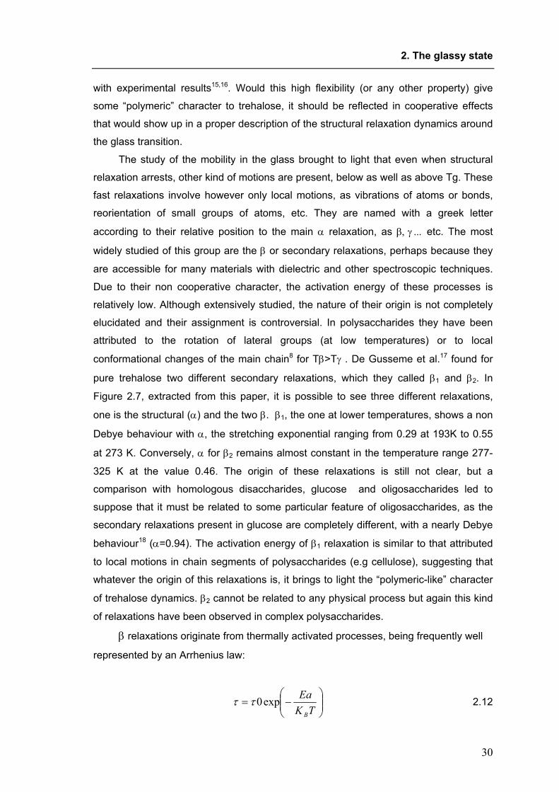
β relaxations originate from thermally activated processes, being frequently well
represented by an Arrhenius law:
−=
TKEa
B
exp0ττ 2.12

2. The glassy state
31
Fig. 2.7- Arrhenius plot of the different relaxations for pure trehalose investigated by
dielectric spectroscopy and temperature-modulated DSC. T=390 K is the calorimetric Tg of
trehalose. The secondary relaxations β1 and β2 show an Arrhenius behaviour for their
characteristic times τ.
The behaviour of this relaxations is generally analogous to the one shown in
figure 9 for trehalose: at low temperatures, the characteristic time of secondary
relaxations becomes more and more divergent, and different relaxations can be
identified and characterised independently. The fact they are referred to as sub-Tg
relaxations reflects they are generally evident at temperatures below Tg away from
primary relaxations. As temperature raises and approaches Tg, relaxations merge and
most of the times are masked by the more intense α structural relaxation.
2.3.5 – Physical ageing
When a liquid is cooled and goes through Tg it forms a glass. If the system is not
cooled enough, structural relaxation generates an evolution of the glass to a more
stable thermodynamic state. As a consequence, the properties of the material change,
i.e a reduction the free volume is seen. This process takes place because of the
presence of molecular motion at temperatures around and below Tg, to at least Tg-50K

2. The glassy state
32
in an observable time scale, and was called physical ageing by Struik19 to distinguish it
from the changes induced by chemical reactions, degradations or changes in
crystallinity, as the effects of this phenomenon should be totally reversible on thermal
cycling. It was already pointed It was already pointed out that this phenomenon is
strongly dependent on control parameters as temperature and pressure, and also on
the intrinsic chemical structure of the material. Therefore a glass near Tg and one 30K
below will age at totally different rates. The technological relevance of ageing comes
out readily, as during this process and due to the structural rearrangements the
physico-mechanical properties (i.e. viscoelasticity, creep, stress-strain, etc) also
change. Many advanced technical materials applications involve the glassy state at a
temperature below Tg. In the field of food and drugs, the stability and properties of the
glassy state have serious implications on the processing and storage. Shelf-life can de
determined by the ageing rate of a material, and some researchers have already tried
to find a connection between this phenomenon and the chemical reactivity of a glass
for applications in drugs20.
Physical ageing had been already noted many years ago, and efforts for its
quantitative treatment can be dated to the early 60’s. Kovacs’ pioneer work21 on
volume relaxations dealt with this phenomenon. Later, physical ageing has been
studied also by means of mechanical techniques (stress-strain, stress-relaxation,
dynamic mechanical and thermo mechanical analysis) and calorimetry.
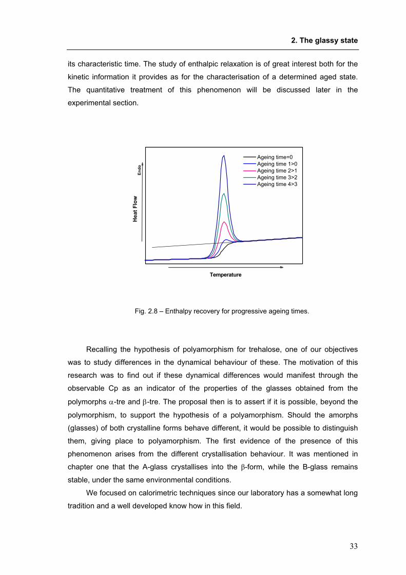
2.3.6 Enthalpy recovery
The changes in properties introduced by the rearrangements during physical
aging can be quantitatively measured through the evolution of a state variable. The
heat capacity is one of the properties affected by aging. The energy minimisation
reached during aging has to be compensated before the system undergoes through the
transformation into a liquid. As a consequence, if energy is added to the material there
will be a more or less regular increase in temperature until the point , in the proximity of
Tg, when part of this energy will be used for breaking the interactions formed during
ageing, what yields an enhancement of the mobility thereafter. In a calorimetric
measurement, this “sink” of enery in represented by an endothermic peak over the
glass transition region, as shown in figure 2.8. As this phenomenon arises as a
consequence of relaxation, it has been also called enthalpic relaxation, or Tg
overshoot. The magnitude of the overshoot peak is determined by the extent of aging,
and it can be studied to obtain precious information about the structural relaxation and
2. The glassy state
33
its characteristic time. The study of enthalpic relaxation is of great interest both for the
kinetic information it provides as for the characterisation of a determined aged state.
The quantitative treatment of this phenomenon will be discussed later in the
experimental section.
Endo
H
eat F
low
Temperature
Ageing time=0 Ageing time 1>0 Ageing time 2>1 Ageing time 3>2 Ageing time 4>3
Fig. 2.8 – Enthalpy recovery for progressive ageing times.
Recalling the hypothesis of polyamorphism for trehalose, one of our objectives
was to study differences in the dynamical behaviour of these. The motivation of this
research was to find out if these dynamical differences would manifest through the
observable Cp as an indicator of the properties of the glasses obtained from the
polymorphs α-tre and β-tre. The proposal then is to assert if it is possible, beyond the
polymorphism, to support the hypothesis of a polyamorphism. Should the amorphs
(glasses) of both crystalline forms behave different, it would be possible to distinguish
them, giving place to polyamorphism. The first evidence of the presence of this
phenomenon arises from the different crystallisation behaviour. It was mentioned in
chapter one that the A-glass crystallises into the β-form, while the B-glass remains
stable, under the same environmental conditions.
We focused on calorimetric techniques since our laboratory has a somewhat long
tradition and a well developed know how in this field.

References for Chapter 2
34
References 1. C.A.Angell INSULATING AND SEMICONDUCTING GLASSES. P Boolchand
(ed.)2000).
2. Comez, L. PhD Thesis. 1996. University of Perugia. Ref Type: Thesis/Dissertation
3. Sussich, F. & Cesaro, A. Transitions and phenomenology of a,a-trehalose polymorphs inter-conversion. Journal of Thermal Analysis and Calorimetry 62, 757-768 (2000).
4. Green, J. L. & Angell, C. A. Phase relations and vitrification in saccharide-water solutions and the trehalose anomaly. Journal of Physical Chemistry 93, 2880-2882 (1989).
5. J.Wong & C.A.Angell Glass structure by Spectroscopy. Marcel Dekler, New York (1976).
6. Gotze, W. LIQUIDS, FREEZING AND THE GLASS TRANSITION. J.-P.Hansen, D.Levesque & J.Zinn-Justin (eds.) (Elsevier,1989).
7. Ngai, K. L. Dynamic and thermodynamic properties of glass-forming substances. Journal of Non-Crystalline Solids 275, 7-51 (2000).
8. Roudaut, G., Simatos, D., Champion, D., Contreras-Lopez, E. & Le Meste, M. Molecular mobility around the glass transition temperature: a mini review. Innovative Food Science & Emerging Technologies 5, 127-134 (2004).
9. Schonhals, A. & Schlosser, E. A new model for the interpretation of the shape of the dielectric relaxation function. Journal of Non-Crystalline Solids 131-133, 1161-1163 (1991).
10. Ngai, K. L. Why the glass transition problem remains unsolved? Journal of Non-Crystalline Solids 353, 709-718 (2007).
11. Franosch, T., Gotze, W., Mayr, M. R. & Singh, A. P. Structure and structure relaxation. Journal of Non-Crystalline Solids 235-237, 71-85 (1998).
12. Alvarez, F., Alegria, A. & Colmenero, J. Interconnection between frequency-domain Havriliak-Negami and time-domain Kohlrausch-Williams-Watts relaxation functions. Phys. Rev. B Condens. Matter 47, 125-130 (1993).
13. Hodge, I. M. Enthalpy relaxation and recovery in amorphous materials. Journal of Non-Crystalline Solids 169, 211-266 (1994).
14. Lindsey, C. P. & Patterson, G. D. Detailed comparison of the Williams--Watts and Cole--Davidson functions. The Journal of Chemical Physics 73, 3348-3357 (1980).
15. Lefort, R., Bordat, P., Cesàro, A. & Descamps, M. Exploring the conformational energy landscape of glassy disaccharides by cross polarization magic angle spinning C13 nuclear magnetic resonance and numerical simulations. II. Enhanced molecular flexibility in amorphous trehalose. Journal of Chemical Physics 126, (2007).
References for Chapter 2
35
16. Lefort, R., Bordat, P., Cesàro, A. & Descamps, M. Exploring conformational energy landscape of glassy disaccharides by cross polarization magic angle spinning 13C NMR and numerical simulations. I. Methodological aspects. The Journal of Chemical Physics 126, 014510 (2007).
17. De Gusseme, A., Carpentier, L., Willart, J. F. & Descamps, M. Molecular mobility in supercooled trehalose. Journal of Physical Chemistry B 107, 10879-10886 (2003).
18. Einfeldt, J., Meisner, D. & Kwasniewski, A. Molecular interpretation of the main relaxations found ID dielectric spectra of cellulose - experimental arguments 33. Cellulose 11, 137-150 (2004).
19. Struik Physical aging in Amorphous polymers and other materials. Elsevier, Amsterdam (1978).
20. Shamblin, S. L., Hancock, B. C. & Pikal, M. J. Coupling between chemical reactivity and structural relaxation in pharmaceutical glasses. Pharmaceutical Research 23, 2254-2268 (2006).
21. A.J.Kovacs Fortschr. Hochpolym.-. Forsch (ed.)1963).

3. DSC experiments
37
3.1 Calorimetry Calorimetry is a technique in which heat flows between the sample and a
reference are measured to determine a variation in chemico-physical properties, or the
temperature at which a certain transition occurs. Typical physical processes studied
(and their relatives changes in enthalpy and specific heat) are fusion, crystallisation,
glass transition, solid-solid transitions (polymorphism) and more generally the evolution
of the specific heat as a function of time or temperature. Other thermal events due to
chemical reactions can be also measured as heat evolution/absorption as a function of
temperature. In modern microcalorimeters, measurements are performed either adding
or subtracting heat to the system and registering the difference in temperature between
the sample and a reference, or measuring the amount of heat necessary to
compensate for the difference in temperature between the sample and the reference.
Experimentally the magnitude registered is the enthalpy variation of the sample against
the reference when both undergo a thermal cycle. Generally, temperature changes
linearly in time defining a scan rate which can go in the most refined instruments from
cents to hundreds of degrees per minute.
The amount of exchanged heat q is measured as a function of time, representing
a power at a given temperature.
Measurements can be visualized as a function of time or temperature, and the
variables represented may be the sample temperature (as a function of time), or the
heat flow. As experiments proceed at normal pressure, and the sample is small
enough, it can be assumed that the material is, at any time, in a condition near
equilibrium. Consequently, the heat flow can be associated with the specific heat at
constant pressure, CP. The latter magnitude is computed by the calorimeter as:
=
tTtqCP
where tq represents the power (heat flow) and tT the scan rate.
Figure 3.1 shows a schematical thermogram with the most typical transitions. The
variable reported as a function of temperature is the heat flow. It is a good practice to
indicate with an arrow the direction of the endothermic processes (e.g fusion). The
DSC schematic diagram corresponds to the thermogram obtained heating a glassy
material which can crystallise when heated to a temperature T > Tg, since the
molecular mobility increases, and the nucleation and growth of crystals becomes

3. DSC experiments
38
feasible. The crystallisation event is represented by an exothermic peak at the
temperature indicated as Tc, since the crystalline state has a lower energy than the
glass. As the system is furtherly heated, an endothermic event occurs, which
corresponds to the fusion of the crystalline material. To signs the temperature at which
the material undergoes local reactions such as decarboxylation, until when, reached a
certain temperature Td, oxidation causes the rupture of molecular bonds, and as a
consequence, the degradation.
Fig. 3.1 Example of a material undergoing different transitions and the thermal events
associated.
Many other methods can be used for the determination of Tg, either by measuring
mechanical or dynamical properties or other thermodynamic properties. Among all type
of measurements, the dilatometric approach has always been considered very tutorial
because changes on the specific volume are directly registered. Dilatometric data are
conceptually simple and easy to analise and the expansion coefficient changes by a
factor of two or three during the transition. However, precision in dilatometric
measurements can be hampered by the preparation of the sample and by the control of
scanning rates on large volumes that are required (in the order of grams), so heating
and cooling rates must be low (in the order of degrees per hours) compared to those
achievable with DSC where samples are of few milligrams1.
3.2 Experimental setup For differential scanning Calorimetry (DSC) the two most widespread instruments
are based on the principles of heat flux or power compensation. We used a power
compensation DSC6 calorimeter, manufactured by Perkin Elmer, for the first part of the
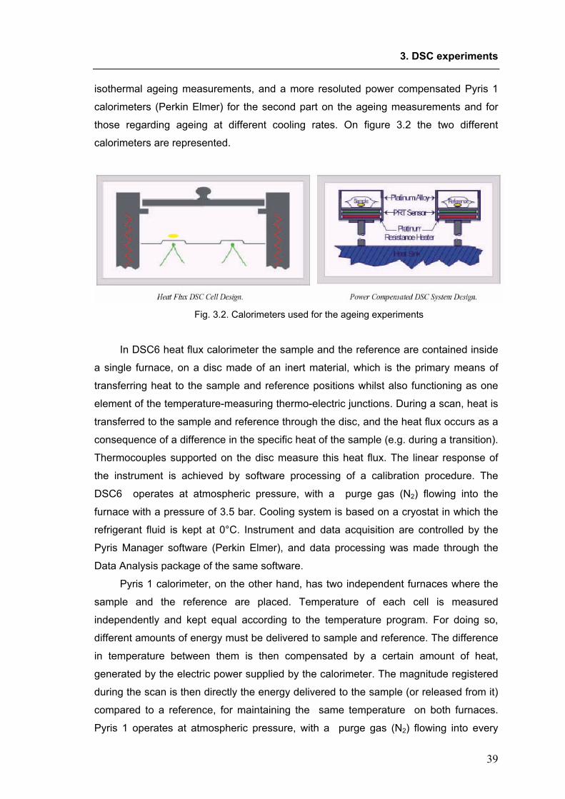
3. DSC experiments
39
isothermal ageing measurements, and a more resoluted power compensated Pyris 1
calorimeters (Perkin Elmer) for the second part on the ageing measurements and for
those regarding ageing at different cooling rates. On figure 3.2 the two different
calorimeters are represented.
Fig. 3.2. Calorimeters used for the ageing experiments
In DSC6 heat flux calorimeter the sample and the reference are contained inside
a single furnace, on a disc made of an inert material, which is the primary means of
transferring heat to the sample and reference positions whilst also functioning as one
element of the temperature-measuring thermo-electric junctions. During a scan, heat is
transferred to the sample and reference through the disc, and the heat flux occurs as a
consequence of a difference in the specific heat of the sample (e.g. during a transition).
Thermocouples supported on the disc measure this heat flux. The linear response of
the instrument is achieved by software processing of a calibration procedure. The
DSC6 operates at atmospheric pressure, with a purge gas (N2) flowing into the
furnace with a pressure of 3.5 bar. Cooling system is based on a cryostat in which the
refrigerant fluid is kept at 0°C. Instrument and data acquisition are controlled by the
Pyris Manager software (Perkin Elmer), and data processing was made through the
Data Analysis package of the same software.
Pyris 1 calorimeter, on the other hand, has two independent furnaces where the
sample and the reference are placed. Temperature of each cell is measured
independently and kept equal according to the temperature program. For doing so,
different amounts of energy must be delivered to sample and reference. The difference
in temperature between them is then compensated by a certain amount of heat,
generated by the electric power supplied by the calorimeter. The magnitude registered
during the scan is then directly the energy delivered to the sample (or released from it)
compared to a reference, for maintaining the same temperature on both furnaces.
Pyris 1 operates at atmospheric pressure, with a purge gas (N2) flowing into every

3. DSC experiments
40
furnace with a pressure of 5 bar. The cooling system is similar to the one described
before, and the software for data acquisition and processing is essentially the same,
differing only in some functionalities enabled or not according to the kind of
measurement performed.
3.3 Materials and methods Trehalose Dihydrate T5251-10g was purchased from Sigma Aldrich and used
without further purification. Sample aluminium pans with 20 µl capacity and covers with
0.1 µm holes were purchased from Perkin Elmer.
3.3.1 Sample preparation For each sample studied, a few milligrams or dihidrate trehalose (TRE h) were
weighted, ranging form 4 to 12 mg, on the Perkin Elmer aluminium sample pans.
Trehalose α and β were prepared in situ (in the calorimeter) according to two different
temperature protocols, in agreement with what already reported in literature2-6
Trehalose α is obtained by dehydration in mild conditions, at low temperatures. Few
milligrams of TRE h sample were weighted in an open sample pan (i.e., without cover)
and heated from 30°C to 142°C with a heating rate of 1°C/min. The thermogram
representing the formation and fusion of the α polymorph, giving rise to the A-
amorphous, can be seen in figure 3.3. Two main events are present, one centered
Figure 3.3 – Formation and fusion of α-trehalose
Fusion of TRE-α
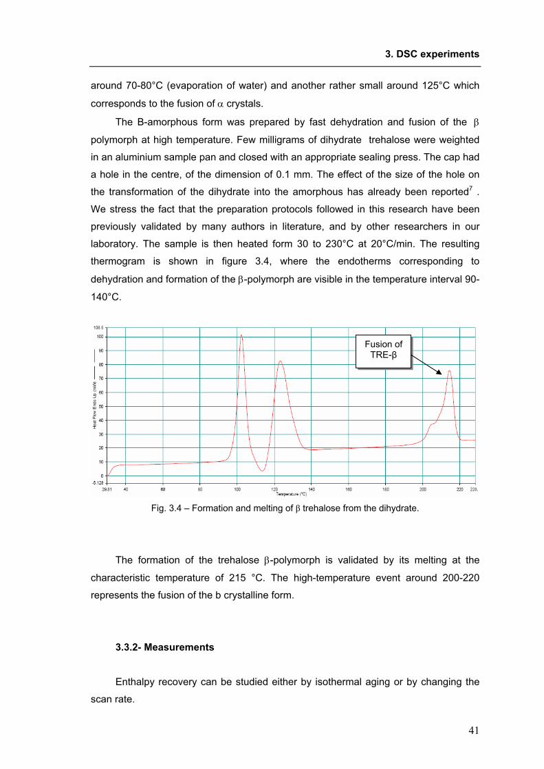
3. DSC experiments
41
around 70-80°C (evaporation of water) and another rather small around 125°C which
corresponds to the fusion of α crystals.
The B-amorphous form was prepared by fast dehydration and fusion of the β
polymorph at high temperature. Few milligrams of dihydrate trehalose were weighted
in an aluminium sample pan and closed with an appropriate sealing press. The cap had
a hole in the centre, of the dimension of 0.1 mm. The effect of the size of the hole on
the transformation of the dihydrate into the amorphous has already been reported7 .
We stress the fact that the preparation protocols followed in this research have been
previously validated by many authors in literature, and by other researchers in our
laboratory. The sample is then heated form 30 to 230°C at 20°C/min. The resulting
thermogram is shown in figure 3.4, where the endotherms corresponding to
dehydration and formation of the β-polymorph are visible in the temperature interval 90-
140°C.
Fig. 3.4 – Formation and melting of β trehalose from the dihydrate.
The formation of the trehalose β-polymorph is validated by its melting at the
characteristic temperature of 215 °C. The high-temperature event around 200-220
represents the fusion of the b crystalline form.
3.3.2- Measurements
Enthalpy recovery can be studied either by isothermal aging or by changing the
scan rate.
Fusion of TRE-β

3. DSC experiments
42
In the first case, the liquid formed by the fusion of one of the crystalline forms is
cooled to a certain temperature Ta (T aging) below Tg and kept there for a time ta.
After that the sample is heated again and the amount of relaxation, represented by the
area of the enthalpic relaxation peak is analysed. The cooling scan rate determines the
initial state of the amorphous formed, and the ageing time the final state. Finally, the
heating scan rate influences the determination of Tg and the position of the event, the
slower the scan rate, the lower the enthalpic recovery finishes.
3.3.2.1 Physical ageing on cooling
This experiments were performed with the Pyris 1 DSC instrument, which allows
good control and stability for cooling rates as low as 0.01 °C/min. The two polymorphs
of trehalose, prepared by the protocols described above, where studied with the same
temperature cycles consisting on different cooling rates and a constant heating rate. In
particular, each trehalose sample was cooled from 140°C to the respective annealing
temperature (87-90-95°C) with the eight following scan rates: 20 – 1 – 0.5 – 0.3 – 0.18
– 0.07 – 0.03 – 0.02 °C/min and heated to 140°C again with a heating rate of 20°C/min.
A scheme is shown in table 3.1.
Ageing on cooling Trehalose A, Trehalose B Cooling Rate (°C/min) 20 1 0.5 0.3 0.18 0.07 0.03 0.02
Heating Rate (°C/min) 20 20 20 20 20 20 20 20
Table 3.1 – Physical ageing on cooling.
All measurements were duplicated, so the reported parameters in the data
analysis section are to be attributed to the mean value between the two analogous
samples.
In the following picture (Fig. 3.5), the different thermal cycles are represented as
an example, for the sample aged cooling until 90°C and then reheating. The higher
baseline curve corresponds to the higher scan rate.
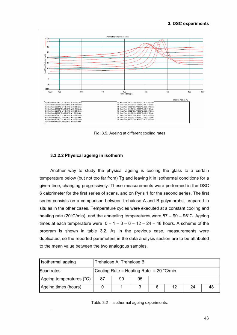
3. DSC experiments
43
Fig. 3.5. Ageing at different cooling rates
3.3.2.2 Physical ageing in isotherm
Another way to study the physical ageing is cooling the glass to a certain
temperature below (but not too far from) Tg and leaving it in isothermal conditions for a
given time, changing progressively. These measurements were performed in the DSC
6 calorimeter for the first series of scans, and on Pyris 1 for the second series. The first
series consists on a comparison between trehalose A and B polymorphs, prepared in
situ as in the other cases. Temperature cycles were executed at a constant cooling and
heating rate (20°C/min), and the annealing temperatures were 87 – 90 – 95°C. Ageing
times at each temperature were 0 – 1 – 3 – 6 – 12 – 24 – 48 hours. A scheme of the
program is shown in table 3.2. As in the previous case, measurements were
duplicated, so the reported parameters in the data analysis section are to be attributed
to the mean value between the two analogous samples.
Isothermal ageing Trehalose A, Trehalose B
Scan rates Cooling Rate = Heating Rate = 20 °C/min
Ageing temperatures (°C) 87 90 95
Ageing times (hours) 0 1 3 6 12 24 48
Table 3.2 – Isothermal ageing experiments.
.

3. DSC experiments
44
Figure 3.6 shows as an example the thermal cycle for one of the trehalose
polymorphs aged at 90°C for different times. The lower enthalpic relaxation
corresponds to the shorter ageing time.
Figure 3.6 – Isothermal ageing at 90°C for progressive times.
A second isothermal aging experiment involves only the A polymorph.
Temperature cycles were performed as before, and ageing proceeded isothermally at
85-90-95 °C. But in this case, before heating again, samples were cooled, immediately
after the annealing, down to a common temperature of 50°C and then heated again
until 143°C, repeating the cycle.
A measurement at an ageing temperature near Tg, in particular at 110°C was
performed to obtain a value of ∆H inf according to the procedure described by
Montserrat8. Finally, a cycle at the ageing temperature of 60°C was performed as a
control of the rate of ageing at temperature values with T-Tg > 50 °C. Table 3.3
represents this part of the experiments.
Isothermal ageing Trehalose A
Scan rates Cooling Rate = Heating Rate = 20 °C/min
Ageing temperatures (°C) 60 85 90 95 110
Ageing times (hours) 0 1 3 6 12 24 48
Table 3.3 – Second part of the ageing experiments
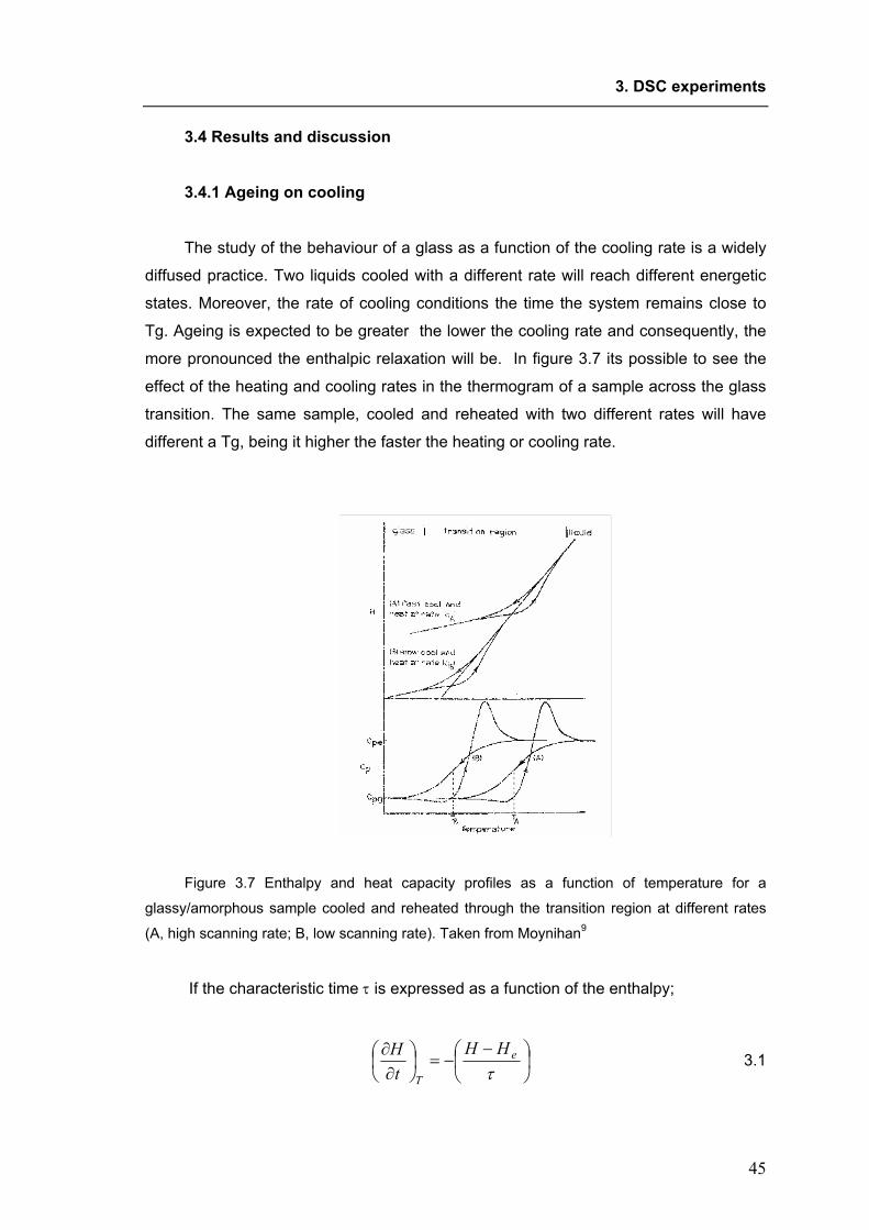
3. DSC experiments
45
3.4 Results and discussion 3.4.1 Ageing on cooling The study of the behaviour of a glass as a function of the cooling rate is a widely
diffused practice. Two liquids cooled with a different rate will reach different energetic
states. Moreover, the rate of cooling conditions the time the system remains close to
Tg. Ageing is expected to be greater the lower the cooling rate and consequently, the
more pronounced the enthalpic relaxation will be. In figure 3.7 its possible to see the
effect of the heating and cooling rates in the thermogram of a sample across the glass
transition. The same sample, cooled and reheated with two different rates will have
different a Tg, being it higher the faster the heating or cooling rate.
Figure 3.7 Enthalpy and heat capacity profiles as a function of temperature for a
glassy/amorphous sample cooled and reheated through the transition region at different rates
(A, high scanning rate; B, low scanning rate). Taken from Moynihan9
If the characteristic time τ is expressed as a function of the enthalpy;
−−=
∂∂
τe
T
HHt
H 3.1

3. DSC experiments
46
where H-He is the deviation of the enthalpy from the equilibrium value in the
liquid, He at a given temperature T, it is evident that τ decreases with increasing
temperature. Thus it is possible to establish three regions according to the conditions:
liquid t∆ >> τ
transition region t∆ ≈ τ
glass t∆ << τ
Now if the scan rate, tT ∆∆ is high, the transition region is shifted to a higher
temperature. As a consequence, the study of the dependence of the Tg from the scan
rate yields information about the relaxation parameter t. It was already pointed out that
the enthalpy relaxation depends on the thermal history of the sample. The enthaly
recovery peak interferes with the accurate determination of Tg on heating, as it masks
the inflection point of the ideal sigmoidal curve representing the transition. However,
Moyhinhan and coworkers established a method for evaluating Tg independently form
the enthalpic relaxation event, as this contribution can be separated analytically9. To
do so, some assumptions must be made. The first one is that the overall enthalpy
relaxation can be considered as the sum of independent relaxations occurring at each
step in temperature:
T
n
i iT tH
tH ∑
=
∂∂
=
∂∂
1 3.2
Second, the difference between equilibrium heat capacities of the liquid and the
glass is nearly constant all over the Tg transformation range considered. Practically,
( )PgPlP CCC −=∆ is known to change, but its variation is so small that this hypothesis
may be considered safe for most glasses.
The third assumption is that the relaxation time τ can be written as.
[ ])(exp)'exp( eii HHcTba −−⋅−⋅=τ 3.3
where b and c are constants, consequently the i relaxation times differ only in
their pre exponential factor, on what is called a temperature independent distribution of
relaxation times.

3. DSC experiments
47
An analogous expression is the one proposed by Narayanaswamy:
∆−⋅
∆
⋅=f
ii RThx
RThxa *).1(exp*expτ 3.4
where ai, ∆h* and x, 0≤ x ≤1 are constants. ∆h* is the activation enthalpy, capable
of describing the evolution of the exponential relaxation times with temperature. An
important parameter in this equation is Tf, the fictive temperature. Tf represents the
temperature at which the ideal glass transition would occur, that is, if the process were
reversible.
Figures 3.8 and 3.9. Physical meaning of the fictive temperature.

3. DSC experiments
48
The meaning of Tf is clear form figure 3.8. A process involving an enthalpy
change ∆H during cooling would follow the path 1. If it were possible to describe a
theoretical path for the same transition, the liquid heat capacity would meet the glass
capacity at a certain temperature Tf .The latter is calculated as the temperature
corresponding to the intersection of the extrapolated curves for the enthalpy of the
liquid and the glass, as shown in figure 3.9. This parameter has the huge advantage of
being independent on the thermal history of the sample. From a thermogram, it can be
calculated from the integral of CP from the relation:
( ) ( )dTCCdTCCTgT
TgT
GlassP
measuredP
Tf
TgT
GlassP
liquidP ∫∫
<<
>>>>
−=− 3.5
as represented in figure 3.9. Tf in a CP measurement can be calculated as the
temperature value where the area between the liquid heat capacity and the
extrapolated glass heat capacity equals that of the experimental curve.
In a linear regime, when H-He is very small, the second exponential in equation
3.3 differs little from 1, so the equation can be expressed:
2*ln)(ln
RThbLim
dTd
T iHeHi eHH
∆−≡−=
=
∂∂
→−ττ 3.6
Considering that under isobaric conditions the enthalpy is a function of
temperature and time:
),( tTHH = and
∂∂
+
∂∂
=dTdt
tH
TH
dTdH
Tt 3.7
where
dTdH
is the total heat capacity and
∂∂
TH
is the heat capacity observed
when temperature is changed instantaneously, and the system has no time to relax.
This can be associated to the glass heat capacity CPG. Introducing the heating or
cooling rate, q, and substituting, eq. 3.6 can be finally rewritten as:
Rh
Tdqd
f
*)/1(
ln ∆−≈ 3.8

3. DSC experiments
49
This equation allows to estimate the *h∆ as the angular coefficient of the
logarithm of the heating or cooling rate as a function of the inverse of Tf.
Borde defined, for liquids approaching the Tg, the fragility parameter m. It
evaluates the variation of a relaxation property in the proximity of the glass transition,
for temperatures T>Tg. m gives an indication of the cooperativity of the relaxation
process, and its analytical form is:
( )
gTT
g
TT
d
dm
→
=τ10log
3.9
It is possible to calculate m from DSC measurements, analogous to the fragility
parameter determined by spectroscopic techniques, but not necessary equal. The
equation is:
RThm
303.2*∆
= 3.10
The amorphous phases A and B were studied as described in table 3, with
different cooling rates and a constant heating rate of 20K/min. The analysis of a
thermogram implies the analysis of every single curve (temperature cycle) in the
following way:
Figure 3.10. Data analysis
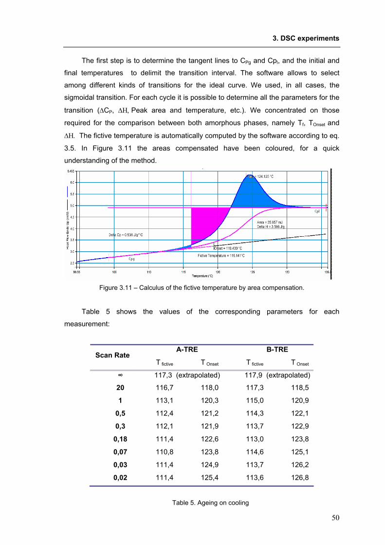
3. DSC experiments
50
The first step is to determine the tangent lines to CPg and Cpl, and the initial and
final temperatures to delimit the transition interval. The software allows to select
among different kinds of transitions for the ideal curve. We used, in all cases, the
sigmoidal transition. For each cycle it is possible to determine all the parameters for the
transition (∆CP, ∆Η, Peak area and temperature, etc.). We concentrated on those
required for the comparison between both amorphous phases, namely Tf, TOnset and
∆Η. The fictive temperature is automatically computed by the software according to eq.
3.5. In Figure 3.11 the areas compensated have been coloured, for a quick
understanding of the method.
Figure 3.11 – Calculus of the fictive temperature by area compensation.
Table 5 shows the values of the corresponding parameters for each
measurement:
A-TRE B-TRE Scan Rate
T fictive T Onset T fictive T Onset
∞ 117,3 (extrapolated) 117,9 (extrapolated)
20 116,7 118,0 117,3 118,5
1 113,1 120,3 115,0 120,9
0,5 112,4 121,2 114,3 122,1
0,3 112,1 121,9 113,7 122,9
0,18 111,4 122,6 113,0 123,8
0,07 110,8 123,8 114,6 125,1
0,03 111,4 124,9 113,7 126,2
0,02 111,4 125,4 113,6 126,8
Table 5. Ageing on cooling

3. DSC experiments
51
The first result comes readily out from the plot of T Onset and T fictive for both
polymorphs (figure 3.12). It is worth noting that eventhough the difference in the
absolute value of each parameter, compared to the analogous for the other polymorph
is not so high, data trend is consistent within each measure.
0.0 0.5 1.0 1.5 2.0 2.5 3.0 3.5 4.0 4.5 5.0 5.5 6.0
110
112
114
116
118
120
122
124
126
TFictive
TOnset
Tre A Tre B
Tem
pera
ture
1/Scan Rate
Figure 3.12. Fictive and onset temperatures for the amorphs A and B trehalose
Temperature behaviour follow a clear trend for T onset as well as for T fictive,
with no random oscillations. For this reason we support the existence of a difference in
the dynamics of the polymorphs. T onset presents the typical increase as the scan rate
decreases, in opposition to T fictive. In the supposition of an ideal transition, with no
enthalpy recovery peak, T fictive ≈T onset. Based on the latter principle, we
extrapolated T fictive and T onset to 0 (infinite scan rate). This corresponds to the two
points reported on the left in figure 3.12.
A further comparison between the two glasses, involving the fragility parameter
m, exposes similar results. The analysis has been made by using equations 3.8-3.10
and the results are reported in figure 3.13 for the two trehalose forms A and B. As in
the previous case, regression analysis demonstrates that the difference between the
amorphous is significative (see the data reported in figure 3.13). The error in the value
of the angular coefficient, *h∆ /R. is less than 7%.

3. DSC experiments
52
0.00258 0.00259 0.00260 0.00261-3.0
-2.5
-2.0
-1.5
-1.0
-0.5
0.0
0.5
o TRE A = 432.1- (166829 +/- 9874)X
log
SR
1/Tf
o TRE B 335.23- (130076 +/- 4802)X
Figure 3.13. Evaluation of the fragility parameter from calorimetric fictive temperature
The values of the fragility parameters m = 183 (±6%) for A-Tre and 143 (±4%) for
B-Tre are then calculated.
These results confirm the existence of two different amorphous phases, gathered
from the fusion and cooling of two different crystalline phases. Not only the
polymorphism is validated with this results, but also the polyamorphism is then
supported.
3.4.2 Isothermal ageing Relaxation phenomena are known to depend strongly also on temperature in
isothermal mode. At a given temperature, the study of the amount of such relaxations
gives an indication on the kinetics of approaching equilibrium in the glassy state.
Several different models have been proposed to deal with non exponentiallity and non
linearity of relaxation parameters. Many of them are based in the equations described
in chapter 2 for structural relaxations. Intuitively is easy to figure out the qualitative
evolution of the thermogram as a function of the ageing time, as the one in figure 3.14.

3. DSC experiments
53
Figure 3.14 Raw experimental data of isothermal aging experiments.
One approach, very diffuse for its simplicity, presumes the calculation of the
hypothetical magnitude of the enthalpy relaxation at a given temperature and infinite
time, hg(∞,Ta). The enthalpy variation at an ageing time t, at the temperature Ta, can
be normalised by the infinite enthalpy to quantify the departure from equilibrium Φ:
Φ = 1- ( ) ( )( )a
aa Th
TthTtZ
,,
1,∞∆
∆−= (0 ≤ Z ≤1 for 0 ≤t ≤ ∞) 3.11
∆h(t, Ta) is calculated as the area between the Cp curves, taking two reference
temperatures, one in the liquid (well above Tg) and one in the glass, well below Tg.
3.12
In principle, ∆h(∞, Ta) can be measured directly from calorimetric measurements,
at temperatures near Tg where this value can be approached (although not reached) in
experimental times; however, it has been shown troublesome in many cases. For this
reason, some authors estimate this parameter assuming a constant specific heat
change, by the relation:
( ) ( )TTCTh gPa −∆≅∞∆ , 3.13
Enthalpic relaxation peak of TRE A at 2880 min
Enthalpic relaxation peak of TRE A at ca. 0 min (first scan)
[ ]∫>
<
−=∆g
g
TT
TTunpagedpaa dTTCTCTth )()(),( )()(
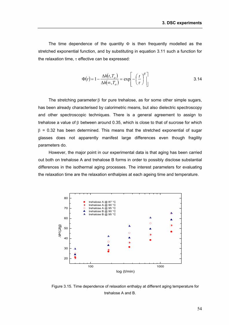
3. DSC experiments
54
The time dependence of the quantity Φ is then frequently modelled as the
stretched exponential function, and by substituting in equation 3.11 such a function for
the relaxation time, τ effective can be expressed:
( ) ( )( )
−=
∞∆∆
−=Φβ
τt
ThTth
ta
a exp,,
1 3.14
The stretching parameter β for pure trehalose, as for some other simple sugars,
has been already characterised by calorimetric means, but also dielectric spectroscopy
and other spectroscopic techniques. There is a general agreement to assign to
trehalose a value of β between around 0.35, which is close to that of sucrose for which
β = 0.32 has been determined. This means that the stretched exponential of sugar
glasses does not apparently manifest large differences even though fragility
parameters do.
However, the major point in our experimental data is that aging has been carried
out both on trehalose A and trehalose B forms in order to possibly disclose substantial
differences in the isothermal aging processes. The interest parameters for evaluating
the relaxation time are the relaxation enthalpies at each ageing time and temperature.
100 1000
20
30
40
50
60
70
80 trehalose A @ 87 °C trehalose A @ 90 °C trehalose A @ 95 °C trehalose B @ 90 °C trehalose B @ 95 °C
∆H (J
/g)
log (t/min)
Figure 3.15. Time dependence of relaxation enthalpy at different aging temperature for
trehalose A and B.
3. DSC experiments
55
Given the number of assumptions above illustrated and the actual quality of data
in some of the experiments, we have not attempted to proceed into calculation of
numerical parameters, but rather to qualitatively present isothermal aging in the form of
relaxation enthalpy of the samples A and B aged at given aging temperatures as a
function of time. These data are reported in figure 3.15 remarking some significant
differences in the aging process of the two trehalose forms.
In conclusion of this short section, we are confident that the experimental results
prove some dynamic difference between the two forms of trehalose A and B, produced
by different protocols. The two protocols can be simply traced back to the undercooled
liquids of the polymorphs trehalose α and β, respectively. Although a larger number of
experimental data in a large range of aging temperature would have provided the
opportunity of fitting the equations above reported, this task will deserve more
experimental time and further attention.

References for Chapter 3
56
References 1. Richardson M. Calorimetry and Thermal Analysis of Polymers. Mathot (ed.) (Carl
Hanser Verlag, Munchen,1994).
2. Akao, K., Okubo, Y., Asakawa, N., Inoue, Y. & Sakurai, M. Infrared spectroscopic study on the properties of the anhydrous form II of trehalose. Implications for the functional mechanism of trehalose as a biostabilizer. Carbohydrate Research 334, 233-241 (2001).
3. Sussich, F., Urbani, R., Cesàro, A., Princivalle, F. & Bruckner, S. New crystalline and amorphous forms of trehalose. Carbohydrate Letters 2, 403-408 (1997).
4. Sussich, F., Urbani, R., Princivalle, F. & Cesàro, A. Polymorphic amorphous and crystalline forms of trehalose. Journal of the American Chemical Society 120, 7893-7899 (1998).
5. Sussich, F. & Cesàro, A. Transitions and phenomenology of a,a-trehalose polymorphs inter-conversion. Journal of Thermal Analysis and Calorimetry 62, 757-768 (2000).
6. Sussich, F., Princivalle, F. & Cesàro, A. The interplay of the rate of water removal in the dehydration of [alpha],[alpha]-trehalose. Carbohydrate Research 322, 113-119 (1999).
7. Sussich, F., Bortoluzzi, S. & Cesàro, A. Trehalose dehydration under confined conditions. Thermochimica Acta 391, 137-150 (2002).
8. Montserrat, S., Cortes, P., Pappin, A. J., Quah, K. H. & Hutchinson, J. M. Structural relaxation in fully cured epoxy resins. Journal of Non-Crystalline Solids 172-174, 1017-1022 (1994).
9. Moynihan, C. T., Easteal, A. J., Wilder, J. & Tucker, J. Dependence of the glass transition temperature on heating and cooling rate. Journal of Physical Chemistry 78, 2673-2677 (1974).

4. BLS experiments
57
SSS OOO UUU RRR CCC EEE (Laser, synchrotron)
ni SS CC AA TT TT EE RR II NN GG VV OO LL UU MM EE
PP OO LL AA RR II SS EE RR
AA NN AA LL YY SS EE RR
θ
nf
q
DDD EEE TTT EEE CCC TTT OOO RRR
4.1 Light scattering
In a scattering experiment a beam of properly polarised light impinges a region of
the sample and is scattered into a detector. The detector is placed at an angle of
interest, the scattering angle θ. Incident photons can either loose or gain energy from
rotational, translational, vibrational and electronic degrees of freedom of molecules.
The electric field of light induces an oscillating polarisation of the electrons in molecules
which at the same time behave as secondary sources of light and as a consequence
radiate (scatter) light. Physically, the instantaneous scattered field can be represented
as the superposition of waves scattered by individual scattering centres, fluctuating as
molecules move. In condensed phases, the presence of destructive interference
between scattered wavelets had to be accounted for. Smoluchowski and Einstein
proposed a model where the fluid is a continuum in which thermal fluctuations originate
local inhomogeneities and as a consequence, density and concentration fluctuations.
The analysis of the time dependence of this fluctuations allows to describe the
structure and dynamics of the system. The frequency shifts, the angular distribution,
the polarisation and the intensity of the scattered light are determined by the size,
shape and molecular interactions of the scattering material1.
4.1.1 Description of the experiment
A scheme of the scattering experiment is shown in figure 4.1, extracted from ref. [1]
ii
nKλπ2
=
=
−=
2sin4 θ
λπinq
KfKiq
Figure 4.1- Schematic scattering experiment f
fnK
λπ2
=
4. BLS experiments
58
The light emitted by the source, most commonly a laser, with wave vector ki
passes through the polarizer to select the polarisation required for the experiment. After
that, part of the radiation with polarisation ni will pass through the sample without
suffering any change, and part will be scattered by the illuminated volume. The beam
scattered at the selected angle and with polarisation nf will reach the detector after
passing through and analyser. The difference between the incident and final wave
vectors will determine the exchanged momentum q. The plane defined by these two
vectors constitutes the scattering plane. The polarisation vectors ni and nf can be
oriented parallel or perpendicular to the scattering plane. When the polarisation is
parallel, it is called H, and V when it is vertical. If the incident light is polarised V and
the diffused light H, the experiment is known as IVH or depolarised scattering.
Conversely when both polarisations are V, IVV is called polarised scattering.The
characteristics of the scattered light depend upon the time scales of the movement of
molecules, thus by means of time correlation functions of the scattered field or intensity
it is possible to achieve a description of such dynamical aspects. The results presented
here correspond to measurements in backscattering configuration, and in the visible
range IVV and IVH where acquired independently for some concentrations.
In the most simple case, the incident light is a plane electromagnetic wave of
wavelength λ, which generates in a point r in space and at a given time t an electric
field Ei(r,t) as follows:
][exp),( 0 trkiEntrE iiii ω−⋅= 4.1
where ωi is the frequency, ni the polarisation, E0 the amplitude and ki the wave
vector.
Assuming light and matter interact weakly, it is possible to describe the scattering
phenomenon by means of the linear response theory, supposing the interaction of light
with matter can be determined knowing how light and matter behave independently
from the presence of each other. Furthermore, the response of one system to the other
is describable in terms of time-correlation functions of dynamical variables1.
4.1.2 Autocorrelation functions
When monitoring the random change in a given property A of a system from the
moment at time t, its value at the moment t+τ will be very close to A(t) if τ is small, but
the difference between A(t) and A(t+ τ) will grow as t becomes large comparing to the

4. BLS experiments
59
period of the fluctuations. This correlation can be expressed by the autocorrelation
function of the property A:
dttAtAT
tAAT
T)()(1
lim)()0(0
τ+⋅= ∫∞→
4.2
The correlation function of a non periodic property decays from 2A to 2A (for
an extensive description of the autocorrelation functions, see ref.[1] as in many
applications it decays like a exponential:
τ
τ tAAA −−+= expAA )()0( 222 4.3
where τ is the “relaxation time” or the correlation time of the property.
Defining the deviation of the instantaneous value of the property A(t) from its
average value as
AtAtA −≡ )()(δ 4.4
it can be demonstrated1 that
2A- )()0( )()0( ττδδ AAAA = 4.5
δA(t) is often called a “fluctuation” since it represents the deviation of the value of
the property from its average value.
In the frequency domain, the spectral density function or power spectrum IE(ω) of
the autocorrelation functions is described as:
)()0(e21 )(I ti
E tEEdt ∗∞
∞−
−⋅= ∫ ω
πω 4.6
where E* is the complex conjugated of E.
)()0( tEE∗ and IE(ω) are the Fourier transform of each other. This means that
measuring one directly allows calculating the other. These quantities are of
fundamental importance since what measured in light scattering experiments is
frequently the autocorrelation function of the electric field scattered by molecules or the
correspondent spectral density.
4. BLS experiments
60
In a classical framework, when an electromagnetic wave perturbs a group of
molecules or atoms in the scattering volume, these get accelerated and, as a
consequence, emit light. Whenever the illuminated region is composed by optically
different sub regions, such is, with a different dielectric constant, scattering will be
verified in other than the forward direction. Local fluctuations in the dielectric constant
take place because molecules are constantly translating and rotating. The scattered
intensity will be proportional to the spectral density of the dielectric constant
fluctuations,
),()0,(e21 )(q,I ti
f tqqdt fifii δεδεπ
ω ω ∗∞
∞−
−⋅∝ ∫ 4.7
In the range energy explored in the experiments of this thesis, the dielectric
fluctuation of wavelengths is considerably larger than intermolecular distances. The
processes contributing to the fluctuations are collective, they involve motions of many
molecules. Then, it is correct to describe them by the laws of macroscopic physics,
hydrodynamics and thermodynamics. The dielectric constant of a pure fluid in
equilibrium is a function of the density ρ and temperature.
4.1.3 Polarised scattering In trehalose, as in many other systems, the greatest contribute to the dielectric
constant fluctuation is due to density fluctuations. Then it becomes necessary to
understand how this fluctuations evolve in time.
Mountain was the first to describe the density fluctuations in terms of
hydrodynamic equations for simple monoatomic liquids, for which transport coefficients
do not depend on frequency, as well as for more complex liquids, where viscoelastic
parameters depend on frequency. The model for calculating the scattered light
supposes that:
a) temperature variations are negligible for the polarizability of molecules is
weakly affected by temperature.
b) concentration gradients are negligible, since homogeneous fluids and
c) density fluctuations are not correlated to orientational fluctuations, for the liquid
is isotropic. The isotropic part of the spectrum of the scattered light then carries all the
information about density fluctuations, and it can be calculated by the double Fourier
transform of the autocorrelation function of the density fluctuations:

4. BLS experiments
61
2)(
),()0,(*).(
q
qqqIISO
δρ
ωδρδρω ∝ 4.8
The second term is called reduced structure factor.
Density fluctuations can be obtained from the linearised hydrodynamic equations
for simple fluids, such as the continuity equation:
00 =⋅∇+∂∂ vt
ρδρ 4.9
the longitudinal part of the Navier-Stokes equation:
)()()(0
02
0
2
vTCC
tv RR ⋅∇∇
+∇−∇−=
∂∂
ρη
δγ
ϕδρ
γρ 4.10
and yet the energy transport equation:
)(1 2
00T
CvtT
tδ
ρλδρ
ϕργδ ∇
+
∂∂
−=
∂∂
4.11
In the last three equations, v is the speed of particles, ρ0 is the equilibrium density
of the fluid, δρ are density fluctuations and δT temperature fluctuations, CR is the speed
of sound at low frequencies,ϕ the thermal expansion coefficient, γ the ratio between
specific heats at constant pressure and temperature: γ=Cp/Cv, and finally, η0 is the
longitudinal viscosity, η0 = 4/3 ηS+ ηΒ, where ηS is the shear viscosity and ηΒ the bulk
viscosity.
For systems where the thermal conductivity is low, as in the case of trehalose,
the hydrodynamic equations can be combined to obtain the following expression2:
0),(002
2
20 =
+
∂∂
+∂∂
tqM
ttqδρη
ρ 4.12
where M0 = ρ0 CR2 is the longitudinal elastic modulus. This equation describes the
temporal evolution of the density fluctuations ),()0,(* ωδρδρ qq .
4. BLS experiments
62
There are three longitudinal modes, which contribute to scattering, and two
transverse modes in a pure liquid, which are purely diffusive shear modes. Among
longitudinal modes, one is a purely diffusive heat-diffusion mode and the remaining two
are propagating modes, due to sound waves. The latter three modes give raise to a
triplet spectrum consisting of a central or Rayleigh line at the incident light frequency ω0
of width determined by the thermal diffusivity and doublets of frequencies ω±ω(q) and
width q2Γ, where Γ is the classical acoustic attenuation coefficient and ±ω(q) (=Csq) are
the Doppler shifts of the scattered light produced by the sound modes, all of which
have adiabatic velocities Cs. This doublet is known as the Brillouin doublet, named
after Leon Brillouin who introduced it on 1914. The position and amplitude depend on
the scatterer. Conversely, in the Rayleigh line, the position of the peak maximum
remains unshifted. The Rayleigh-Brillouin spectrum arises from the inelastic interaction
between a photon and the hydrodynamic modes of a fluid. The photon may gain or lose
energy from the phonons or sound modes in the fluid and as a consequence are
shifted in frequency to ± ω(q). The resultant Brillouin doublet can be regarded as the
Stokes and anti-Stokes translational spectrum of the liquid. The width of the bands
reflect the lifetime ( q2Γ )-1 of a classical phonon of wave vector q. The Rayleigh line,
conversely, represents the entropic or heat fluctuations contribution to the scattering,
which are purely diffusive or dissipative modes of the fluid. Landau and Placzek
proposed that the ratio of the intensity of the Rayleigh line to that of the Brillouin
doublet should equal the ratio of the heat capacities. The latter relation is known as the
Landau-Placzek ratio.
CvCvCp
II
B
R −= 4.13
However, it must be noted that to determine the width of the central line is a
delicate task and requires high resolution measurement as DTq2 is usually less than 10-
7 sec. Moreover, the presence of impurities (e.g powder) derived from sample
preparation will contribute to the intensity of the scattered light in this region, altering
the results.
Assuming that density fluctuations can be described by simple linearised
hydrodynamic equations and that widths are small compared to the shifts, the following
expression for the density fluctuations can be gathered1:
4. BLS experiments
63
+Γ−+−⋅
−= tqtqtDq
qqtqq
Tl
l )(cosexp1exp11)0,()0,(*),()0,(* 22 ω
γγδρδρδρδρ
tω(q)tΓqb(q)γ
sinexp1 2−+ 4.14
where b is
−Γ≡
CsD
b V
γ3
φ ; TD is the thermal diffusivity coefficient, Dv the longitudinal
kinematic viscosity defined as: 0
34
ρ
ηη
mD
SB
V
+
= ; P
T CmD
0ρλ
=
These are “diffusion coefficients” accounting for the diffusion of momentum and
heat, respectively.
The corresponding spectral density is obtained by Fourier transforming the latter
equation, what yields:
[ ] [ ] [ ] [ ] [ ]
+
Γ++
Γ+
Γ+−
Γ+
+
−∝ 222
2
222
2
222
2
)()(
111),(qq
q
q
qD
qDqST
T
ωωωωγωγωρρ
[ ][ ] [ ]
[ ][ ] [ ]
Γ+−
−−
Γ++
+222222 )(
)(
)(
)()(1
q
qqbωω
ωω
ωω
ωωγ
4.15
Thus, the scattering spectrum can be represented by a sum of Lorentzian
functions. The last term is generally difficult to observe. The first term represents the
Rayleigh line, which is a Lorentzian functions with half width at half maximum
∆ωc(q) = DT q2 = (λ/mρ0CP)q2 4.16
The next two terms represents the Brillouin doublets, which are two Lorentzians
symmetrically shifted at ± ω(q) = ± Csq, and their half width at half maximum is:

4. BLS experiments
64
( ) 2
00
2 134
21)( q
Cmmqq
P
SB
B
−
+
+
=Γ=∆ργλ
ρ
ηηω 4.17
The last two terms of equation 4.15 represent a non-Lorentzian correction to the
Brillouin doublet. These terms shift the Brillouin peaks and their position in the
spectrum becomes no longer symmetric. Fortunately, this correction is usually very
small and can be neglected. Rearranging eq. 4.15 and neglecting the last two terms,
yields:
[ ] [ ] [ ]222
22
222
2
2)(
)(22111),(qq
qD
qDqSBB
BB
T
T
Γ+−
Γ+
+
−∝
ωωω
ωγωγ
ωρρ 4.18
where ΓB and ωB are the Brillouin characteristic amplitude and frequency,
respectively. If the parameter γ is set to 1, (CP = Cv) the first term becomes null and the
second term resembles the equation of a mass oscillating in a dissipative medium,
after what it is named the Damped Harmonic Oscillator function (DHO).
[ ] [ ]222
22
)(
)(),(
qqqS
BB
BB
Γ+−
Γ∝
ωωω
ωωρρ 4.19
This equation allows the traditional acoustic analysis of the scattering spectrum
to determine the shift (ω) and the width (Γ) of the Brillouin peaks, the analogous to the
period and amplitude of the oscillation damped by thermal diffusion and viscous
dissipation. This two parameters, used in the framework of a proper model, give the
first characterization of the system as a function of its dissipative (Γ) and propagating
components (ω).
4.2 IUVS and VIS experiments
It is clear from chapter 4.1 that measuring the intensity in a scattering experiment
is a step towards the characterisation of the dynamic properties of the system. Different
models, ranging from the simple DHO to the more complex viscoelastic one, can be
applied to describe the system in terms of attenuation and propagation in the first case,
and of the dynamic transport coefficients in the second case. It is obvious that the
4. BLS experiments
65
complexity of the viscoelastic model requires a careful choice of the memory function
and macroscopic transport and thermodynamic coefficients. The strength of this model
is the huge amount of information it can reveal, but its weakness relies on the
numerous parameters necessary for the fitting procedure. This problem is usually
overcome acquiring spectra in the same experimental conditions (concentration and
temperature) in different energy regions, and fitting them simultaneously. In this way,
free parameters are tightly constrained and can be inferred with a certain accuracy.
BLS has the advantage of accessing a wide range of frequencies. In some
systems it is possible to see with this technique alone the transition between the
adiabatic to the intermediate regime, or the high frequency response, depending on the
intrinsic characteristics of the studied material. Unfortunately, this was not the case for
trehalose-water solutions. In a solution the dynamics are affected by the contribution of
each component, plus the contribution of the interaction solute-solvent couple, which
adds another degree of complexity. A diluted solution would be expected to have a
strong water-like behaviour, with little contribution of the sugar. As sugar content
increases, some water molecules will interact closely with the solute as the hydration
sphere, and water dynamics will be the resultant of the contribute of hydration plus
bulk, free water. When entering the concentrated regime, bulk water disappears and
the principal component is hydrated sugar. Our experiments concentrate in this
situation, as well as the bulk water - hydrated sugar one.
4.2.1 Fitting parameters
Many substances of industrial interest have been fully characterised during years,
their static coefficients being reported in literature. This is obviously not the case for
sugars. Sucrose has been of some interest since it is present in so many large scale
food production processes. The whole process control, dimension and standardisation
requires a good knowledge of the evolution of the system’s parameters in a wide range
of temperature, concentrations and is some cases pressure. For the latter reason there
is a relevant amount of data on sucrose in literature, still many data refer to
fundamental properties that are not strictly related to the parameters of interest for the
equations reported in section 4.1. The situation is even much less lucky with trehalose,
for the spotlights fell on this molecule mainly in the middle 90’s, with the wave of the
first sensationalist papers (many based on wrong data, see the comments to Sola
Penna’s article in chapter 1) yelling to the world the “exceptional” properties of the

4. BLS experiments
66
disaccharide. The growth of the myth biased many results, and we faced the problem
of confronting controversial results on the same system (concentration and range of
temperature) which led no other options than to choose the most reasonable one.
Regarding thermodynamic variables, it is in general a good first approximation to use
the corresponding data for sucrose. In the case of transport coefficients this
approximation gets weaker as the system concentrates, so values for trehalose are
needed. Parameters as the refraction index n and density ρ where considered enough
similar to those of sucrose at a first approximation, but we would realise that small
deviations in n greatly influenced our results. While good quality density data for
trehalose were available in literature, but refraction index references were inexistent
and it became necessary to measure it. An original setup was conceived and
implemented on the IUVS beamline, based on a modification of the fixed angle of
incidence method for a hollow prism3 to measure the refraction index as a function of
temperature, wavelength and concentration.
4.2.2 Experimental setup
Scattering experiments were performed mainly on trehalose solutions, at two
facilities operating in different spectral ranges. In IUVS experiments, carried out at the
Elettra synchrotron facility in Trieste, the incident radiation has a wavelength of 244 nm
(ultraviolet). VIS experiments were performed at the University of Perugia with the
GHOST group, in the laboratory of prof. Daniele Fioretto. The source operated at 532
nm (green light). In both facilities, the backscattering configuration was used. At IUVS,
V spectra were acquired for a traditional acoustic analysis. At Perugia instead, VV (for
all concentrations) and VH (for two of them) were acquired for calculating the isotropic
spectrum.
4.2.2.1 IUVS Beamline
IUVS experiments were performed at the Inelastic UltraViolet Scattering
beamline, at the Elettra Synchrotron radiation Laboratory in Trieste. A schematic
representation is shown in figure 4.2. The energy region probed by this relatively new
beamline renders it unique, as it is situated between conventional BLS (10-6 nm-1≤ q ≤
10-2 nm-1) and INS or IXS (Inelastic neutron scattering or X-ray scattering, 1 nm-1 ≤ q ≤
102 nm-1). Some characteristic features of the mesoscopic dynamics have been
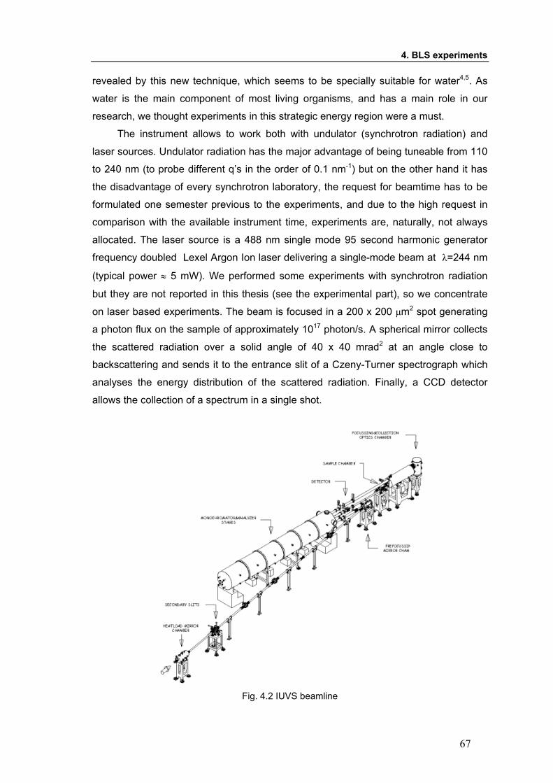
4. BLS experiments
67
revealed by this new technique, which seems to be specially suitable for water4,5. As
water is the main component of most living organisms, and has a main role in our
research, we thought experiments in this strategic energy region were a must.
The instrument allows to work both with undulator (synchrotron radiation) and
laser sources. Undulator radiation has the major advantage of being tuneable from 110
to 240 nm (to probe different q’s in the order of 0.1 nm-1) but on the other hand it has
the disadvantage of every synchrotron laboratory, the request for beamtime has to be
formulated one semester previous to the experiments, and due to the high request in
comparison with the available instrument time, experiments are, naturally, not always
allocated. The laser source is a 488 nm single mode 95 second harmonic generator
frequency doubled Lexel Argon Ion laser delivering a single-mode beam at λ=244 nm
(typical power ≈ 5 mW). We performed some experiments with synchrotron radiation
but they are not reported in this thesis (see the experimental part), so we concentrate
on laser based experiments. The beam is focused in a 200 x 200 µm2 spot generating
a photon flux on the sample of approximately 1017 photon/s. A spherical mirror collects
the scattered radiation over a solid angle of 40 x 40 mrad2 at an angle close to
backscattering and sends it to the entrance slit of a Czeny-Turner spectrograph which
analyses the energy distribution of the scattered radiation. Finally, a CCD detector
allows the collection of a spectrum in a single shot.
Fig. 4.2 IUVS beamline
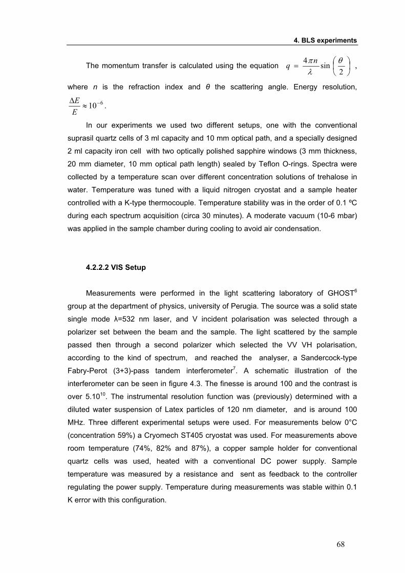
4. BLS experiments
68
The momentum transfer is calculated using the equation
=
2sin4 θ
λπ nq ,
where n is the refraction index and θ the scattering angle. Energy resolution,
610−≈∆EE
.
In our experiments we used two different setups, one with the conventional
suprasil quartz cells of 3 ml capacity and 10 mm optical path, and a specially designed
2 ml capacity iron cell with two optically polished sapphire windows (3 mm thickness,
20 mm diameter, 10 mm optical path length) sealed by Teflon O-rings. Spectra were
collected by a temperature scan over different concentration solutions of trehalose in
water. Temperature was tuned with a liquid nitrogen cryostat and a sample heater
controlled with a K-type thermocouple. Temperature stability was in the order of 0.1 ºC
during each spectrum acquisition (circa 30 minutes). A moderate vacuum (10-6 mbar)
was applied in the sample chamber during cooling to avoid air condensation.
4.2.2.2 VIS Setup
Measurements were performed in the light scattering laboratory of GHOST6
group at the department of physics, university of Perugia. The source was a solid state
single mode λ=532 nm laser, and V incident polarisation was selected through a
polarizer set between the beam and the sample. The light scattered by the sample
passed then through a second polarizer which selected the VV VH polarisation,
according to the kind of spectrum, and reached the analyser, a Sandercock-type
Fabry-Perot (3+3)-pass tandem interferometer7. A schematic illustration of the
interferometer can be seen in figure 4.3. The finesse is around 100 and the contrast is
over 5.1010. The instrumental resolution function was (previously) determined with a
diluted water suspension of Latex particles of 120 nm diameter, and is around 100
MHz. Three different experimental setups were used. For measurements below 0°C
(concentration 59%) a Cryomech ST405 cryostat was used. For measurements above
room temperature (74%, 82% and 87%), a copper sample holder for conventional
quartz cells was used, heated with a conventional DC power supply. Sample
temperature was measured by a resistance and sent as feedback to the controller
regulating the power supply. Temperature during measurements was stable within 0.1
K error with this configuration.
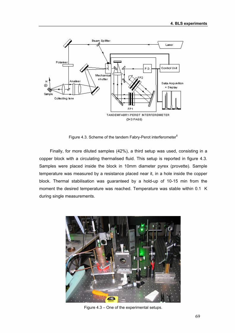
4. BLS experiments
69
Figure 4.3. Scheme of the tandem Fabry-Perot interferometer6
Finally, for more diluted samples (42%), a third setup was used, consisting in a
copper block with a circulating thermalised fluid. This setup is reported in figure 4.3.
Samples were placed inside the block in 10mm diameter pyrex (provette). Sample
temperature was measured by a resistance placed near it, in a hole inside the copper
block. Thermal stabilisation was guaranteed by a hold-up of 10-15 min from the
moment the desired temperature was reached. Temperature was stable within 0.1 K
during single measurements.
Figure 4.3 – One of the experimental setups.
4. BLS experiments
70
4.2.3 Materials and methods Trehalose dihydrate was purchased from Sigma Aldrich. Several lots and
samples produced by different suppliers were tried before finding the one that would
meet the characteristics required for the IUVS experiments. The main problem was the
metal content that, although not declared, was present and gave rise to fluorescence
when illuminated with UV light at 244 nm. A description of the tests and of the
procedures is provided for benefit of future experiments.
4.2.3.1 Pre-treatments
The first test carried out was the absorption characterisation of samples in the UV
range. In principle, UV absorption of aqueous sugar solutions should be zero down to
the far UV absorption bands of the oxygen, although some turbidity is often observed at
low wavelength. By using a spectrophotometer (Cary 4E UV-VIS spectrophotometer)
the absorbance was around what specified by the producer and did not interfere with
the measurements. However, a further characterisation with a spectrofluorimeter
(Perkin Elmer LS 50 B) showed out typical metallic emissions that could be found also
in samples declared to have reduced metal ion content for undergone ionic exchange
chromatography. Since at the beginning some IUVS measurements were performed as
well on maltose and sucrose, also these sugars were characterised. Maltose M9171
from Sigma Aldrich had the same problem than trehalose. Sucrose (p.n. 365157) from
Carlo Erba had absorbance problems and some emission from organic impurities. This
suggested that although the sample was white to the eye, probably some anthocyanin
or other natural colorant, could remain from the plant from which sucrose was extracted
after the purification. Organic dye molecules are generally soluble in ethanol, therefore
a purification with ethanol was carried out. Recrystallisation is widely known in
chemistry as one of the simplest ways to purify a sample. The principle of his technique
consists in the dissolution of the sample in a “good” solvent and the selective
precipitation of the compound of interest, either by decreasing the temperature below
the saturation or by addition of a “bad” co-solvent to facilitate the crystallization.
Therefore, the concentration of the solution is usually as high as possible, that is, near
the saturation to approach easily the critical concentration. Impurities trapped in (or
stacked superficially on) the original crystals are dispersed and solubilised in the
solution step. In our case, about 500 gr of sucrose were dissolved in 500 ml of
deionised MilliQ water, and the solution was heated up to around 50°C to facilitate the

4. BLS experiments
71
complete dissolution (the actual solubility would allow up to about 1300 g). The viscous
and dense solution was filtered through a gouch filter and then poured gradually in 1.5 l
of cold ethanol (kept at -30°C until some minutes before) gently stirred with a magnet.
Ethanol is a poor solvent for all sugars (in this solvent, it is curious to note that sucrose
is slightly more soluble than trehalose). Upon mixing with the non-solvent alcoholic
phase, altogether with the drop in temperature, the instantaneous precipitation of very
tiny crystals of sugar is induced. The solution was then filtered either with a gouch filter
connected to a water pump, or –for small volume preparations- with a disposable
Stericup Millipore filter with 0.45 µm pore diameter, 250 ml capacity connected to a
vacuum pump. The crystalline precipitate was collected and poured on partially opened
(covered but not hermetically closed) Petri dishes let in oven at 60°C for at least 48
hours. The procedure was repeated twice or three times depending on the desired
quality of the purified sample.
This treatment worked quite well for sucrose, since as it was mentioned before,
impurities were essentially organic. In the case of trehalose, it did not show to be that
useful. In general, trehalose had lower yields than sucrose, probably due to the slower
crystallisation rate of the di-hydrate polymorph that is obtained in aqueous mixed
solvents. Moreover (and perhaps for this reason), metals remained still trapped in the
crystals and were not dispersed into the filtered solution. Although, absorbance due to
organic impurities diminished in a significative manner, emitted fluorescence did not.
Therefore an alternative solution had to be explored, by choosing a protocol which
used a specific chelant to complex metals in a form that is soluble in organic solvents.
In the meantime, we were aware of the commercialisation of a new sample of trehalose
obtained by biotechnological treatment from starch which in the analysis showed very
low metal fluorescence emission, so this lot was adopted for the measurements. It is
worth mentioning that fluorescence is not among the characteristics provided in the
technical note of trehalose nor available from the dealer (i.e., Sigma) upon request.
So if not otherwise specified, sucrose in the experiments was a purified (double
crystallised) sample from Carlo Erba (product number 365157) and trehalose was from
a Sigma product (either T5251 or T9449).
Some words are also necessary about the third sugar originally taken into
consideration in the present study, i.e. maltose. Several samples of maltose showed
high metal content which interfered dramatically with the experiments. The purification
procedure for this sugar was also time and resources consuming, but, more important,
we were not certain of having enough available instrument time at our disposition to
carry a full concentrations range comparative analysis of homologous disaccharides,
which happened to be true at the end. For these and other reasons, experiments on

4. BLS experiments
72
maltose were cancelled and the time available for measurements was dedicated
preferentially to trehalose, in search of an exhaustive time-temperature characterisation
of this system.
4.2.3.2 Sample preparation
Sugar solutions, of different concentrations, were obtained by dissolution of a
weighted amount of sugar in a weighted amount of water. We chose not to work with
volumetric fractions to prevent corrections of the concentration with temperature. It is
relevant to recall here that sucrose crystalline powder is in the anhydrous form,
whereas trehalose crystalline powder is commonly prepared as “di-hydrate” form. Not
only this fact had to be taken properly into account for the simple calculation of the
mixed-system concentration (sugar-water) but also introduces a number of non-
obvious problems when preparing the solutions for the experiments. The most
important one comes from the large difference in solubility: while sucrose solubility in
water at 20 °C is of about 2 g of sugar per g of water, that of trehalose (as dihydrate
form) is only about 0.5 g of sugar per g of water. Therefore, it is not surprising that
sucrose solutions were prepared without any problem. For the most concentrated
solutions, heating enhanced dissolution, and then the cooled samples (over-saturated)
remained stable all over measurement times.
Trehalose was quite more troublesome. Dilute or moderately concentrated
samples up to the saturation limit (0-70%) were prepared as sucrose. For more
concentrated solutions, another procedure had to be adopted. After several
unsuccessful tentatives (and many broken quartz cells!) it was evident that preparing
these samples by adding little amount of water to the crystalline solid was not a clever
choice. We would infer that for some reason the theoretical state diagram for trehalose
did not reflect the actual heterogeneous changes occurring in macroscopic samples. In
other words, few millilitres of sample in the rectangular quartz cuvette composed by,
let’s say, 2.5 grams or more of trehalose with 0.5 grams of water were let in oven at
60°C seeking for achieving dissolution. This system showed and heterogeneous
behaviour. The water volume added (0.5 grams do not wet all the powder but only a
little part of it. The sample was then composed by a zone of dry powder, which
remained unchanged even after one week, and a water-rich zone. As a consequence,
this abundant water eventually caused crystallisation nuclei and further crystalline
growing up to the fracture of the quartz cell. The water-trehalose concentration in
equilibrium with the di-hydrate composition is at 90.5% (w/w) of trehalose. Therefore
4. BLS experiments
73
initial crystallisation further facilitates crystalline growing because of decreasing
viscosity of the medium. In conclusion, the readily crystallisation of trehalose was a
serious constraint we faced the whole research through.
A better result for achieving highly concentrated samples was obtained by
preparing moderately concentrated solutions (not more than 70% (w/w) of trehalose),
heating until uniformly clear (around 100°C) and then evaporating the excess water
until reaching approximately the desired concentration (calculated by weight). We
noticed, as some other researchers working with concentrated solutions of trehalose 8
that the apparent boiling point of the system showed a steep increase when
approaching the dihydrate concentration (an analysis of the thermal transitions of the
several trehalose polymorphs has been made elsewhere, see for example the papers
by Sussich and the recent review published in Food Chemistry 2008 in the Annex,
Chapter 6). However, upon progressively increasing trehalose content water
evaporation was more and more difficult. Above 80% weight concentration, it was
necessary to heat over 130°C, otherwise an increase of 1% concentration would not
occur even in 5 or 6 hours. Admittedly, at least the solution was nice to see: when the
temperature is high, convective motions are not enough to give an homogeneous fluid.
Hot masses (with higher content of more mobile water?) from the bottom go up in what
seems a rather laminar flow. When they get in contact with the upper interface, and as
air or vapour bubbles escape from the fluid, a sort of “film” forms at the interface. At this
point two things may happen. If the container (e.g quartz cell) is hot, the film (or more
parallel films) go up like the piston of a syringe, they do not deform or break, and they
break only when they get in contact with the colder teflon cap of the cell. Conversely if
the cell walls are colder than the liquid (e.g the cell is heated only at the bottom) the
film seems to stuck at the walls and its centre moves up and down as the liquid moves
below it. The interesting thing is that when moving, the surface of the film gets
patterned, resembling a spider net, small visible pieces seem to compare as the film is
stretched by the pressure of vapour. When looking at it, I wondered many times if this
effect was somehow related to bioprotection. In my opinion (and I emphasize my
opinion, leaving my tutors out) it is (or it may provide some hints to), that is why I
described it here. I do not have the knowledge to relate what observed to a measurable
property, but in my impression trehalose prevents water from escaping abruptly (at
moderate temperatures, below 130°C).
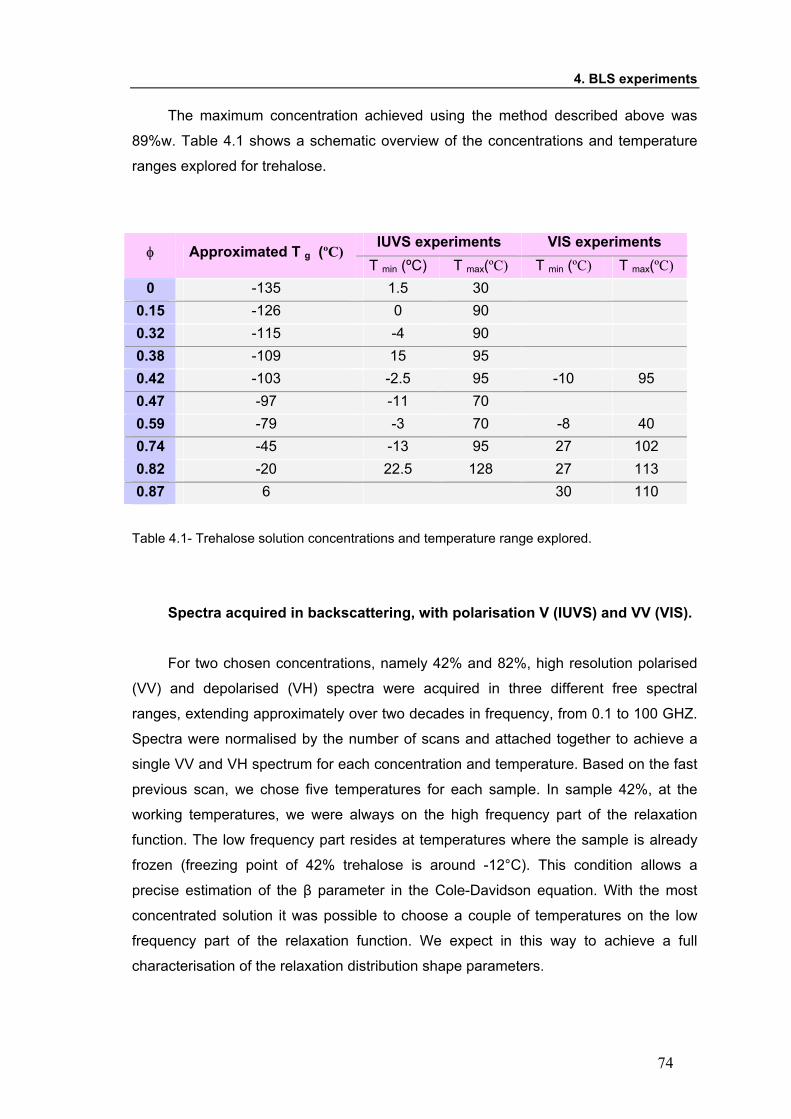
4. BLS experiments
74
The maximum concentration achieved using the method described above was
89%w. Table 4.1 shows a schematic overview of the concentrations and temperature
ranges explored for trehalose.
IUVS experiments VIS experiments φ Approximated T g (ºC)
T min (ºC) T max(ºC) T min (ºC) T max(ºC) 0 -135 1.5 30
0.15 -126 0 90 0.32 -115 -4 90 0.38 -109 15 95 0.42 -103 -2.5 95 -10 95 0.47 -97 -11 70 0.59 -79 -3 70 -8 40 0.74 -45 -13 95 27 102 0.82 -20 22.5 128 27 113 0.87 6 30 110
Table 4.1- Trehalose solution concentrations and temperature range explored.
Spectra acquired in backscattering, with polarisation V (IUVS) and VV (VIS). For two chosen concentrations, namely 42% and 82%, high resolution polarised
(VV) and depolarised (VH) spectra were acquired in three different free spectral
ranges, extending approximately over two decades in frequency, from 0.1 to 100 GHZ.
Spectra were normalised by the number of scans and attached together to achieve a
single VV and VH spectrum for each concentration and temperature. Based on the fast
previous scan, we chose five temperatures for each sample. In sample 42%, at the
working temperatures, we were always on the high frequency part of the relaxation
function. The low frequency part resides at temperatures where the sample is already
frozen (freezing point of 42% trehalose is around -12°C). This condition allows a
precise estimation of the β parameter in the Cole-Davidson equation. With the most
concentrated solution it was possible to choose a couple of temperatures on the low
frequency part of the relaxation function. We expect in this way to achieve a full
characterisation of the relaxation distribution shape parameters.
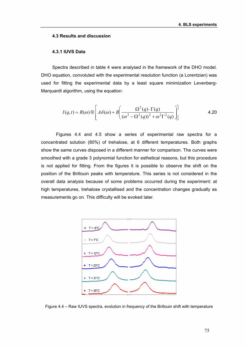
4. BLS experiments
75
4.3 Results and discussion 4.3.1 IUVS Data Spectra described in table 4 were analysed in the framework of the DHO model.
DHO equation, convoluted with the experimental resolution function (a Lorentzian) was
used for fitting the experimental data by a least square minimization Levenberg-
Marquardt algorithm, using the equation:
Γ+Ω−Γ⋅Ω
+⊗=)())((
)()()()(),( 22222
2
qqqqBARtqIωω
ωδω 4.20
Figures 4.4 and 4.5 show a series of experimental raw spectra for a
concentrated solution (80%) of trehalose, at 6 different temperatures. Both graphs
show the same curves disposed in a different manner for comparison. The curves were
smoothed with a grade 3 polynomial function for esthetical reasons, but this procedure
is not applied for fitting. From the figures it is possible to observe the shift on the
position of the Brillouin peaks with temperature. This series is not considered in the
overall data analysis because of some problems occurred during the experiment: at
high temperatures, trehalose crystallised and the concentration changes gradually as
measurements go on. This difficulty will be evoked later.
T = -8°C
T = 35°C
T = 23°C
T = 12°C
T = 7°C
T = 31°C
Figure 4.4 – Raw IUVS spectra, evolution in frequency of the Brillouin shift with temperature
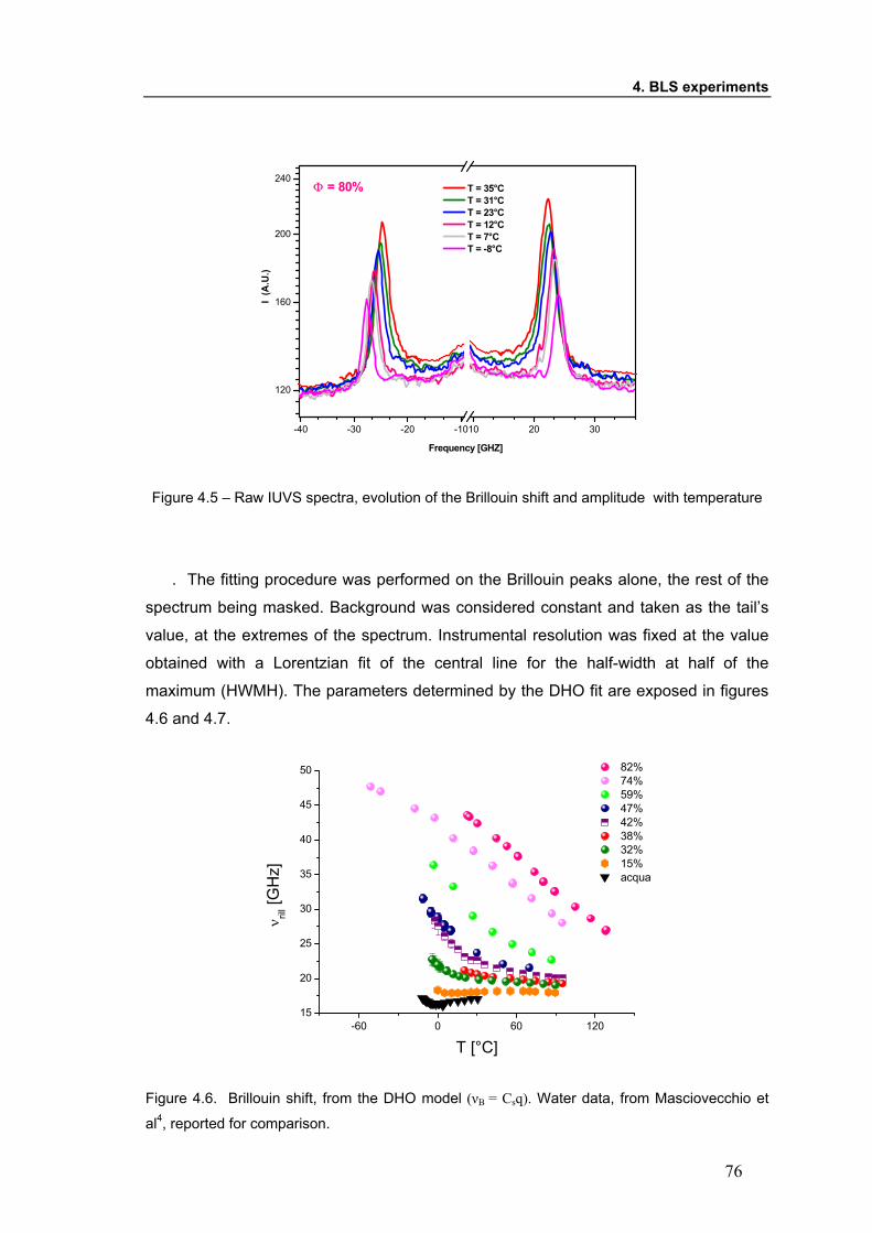
4. BLS experiments
76
-40 -30 -20 -1010 20 30
120
160
200
240Φ = 80% T = 35°C
T = 31°C T = 23°C T = 12°C T = 7°C T = -8°C
I (A
.U.)
Frequency [GHZ]
Figure 4.5 – Raw IUVS spectra, evolution of the Brillouin shift and amplitude with temperature
. The fitting procedure was performed on the Brillouin peaks alone, the rest of the
spectrum being masked. Background was considered constant and taken as the tail’s
value, at the extremes of the spectrum. Instrumental resolution was fixed at the value
obtained with a Lorentzian fit of the central line for the half-width at half of the
maximum (HWMH). The parameters determined by the DHO fit are exposed in figures
4.6 and 4.7.
-60 0 60 12015
20
25
30
35
40
45
50
ν rill [G
Hz]
T [°C]
82% 74% 59% 47% 42% 38% 32% 15% acqua
Figure 4.6. Brillouin shift, from the DHO model (νB = Csq). Water data, from Masciovecchio et
al4, reported for comparison.
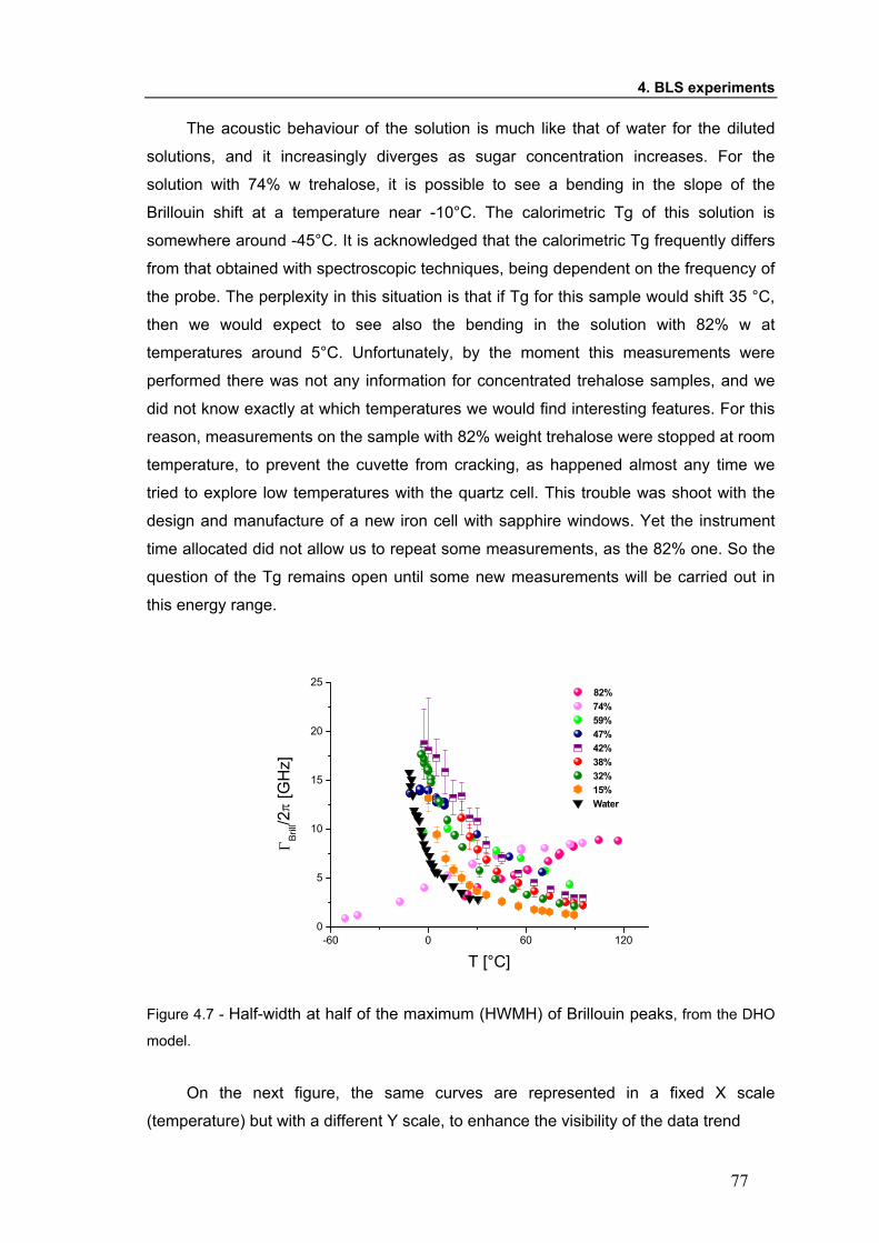
4. BLS experiments
77
The acoustic behaviour of the solution is much like that of water for the diluted
solutions, and it increasingly diverges as sugar concentration increases. For the
solution with 74% w trehalose, it is possible to see a bending in the slope of the
Brillouin shift at a temperature near -10°C. The calorimetric Tg of this solution is
somewhere around -45°C. It is acknowledged that the calorimetric Tg frequently differs
from that obtained with spectroscopic techniques, being dependent on the frequency of
the probe. The perplexity in this situation is that if Tg for this sample would shift 35 °C,
then we would expect to see also the bending in the solution with 82% w at
temperatures around 5°C. Unfortunately, by the moment this measurements were
performed there was not any information for concentrated trehalose samples, and we
did not know exactly at which temperatures we would find interesting features. For this
reason, measurements on the sample with 82% weight trehalose were stopped at room
temperature, to prevent the cuvette from cracking, as happened almost any time we
tried to explore low temperatures with the quartz cell. This trouble was shoot with the
design and manufacture of a new iron cell with sapphire windows. Yet the instrument
time allocated did not allow us to repeat some measurements, as the 82% one. So the
question of the Tg remains open until some new measurements will be carried out in
this energy range.
-60 0 60 1200
5
10
15
20
25
Γ Bril
l/2π
[GH
z]
T [°C]
82% 74% 59% 47% 42% 38% 32% 15% Water
Figure 4.7 - Half-width at half of the maximum (HWMH) of Brillouin peaks, from the DHO
model.
On the next figure, the same curves are represented in a fixed X scale
(temperature) but with a different Y scale, to enhance the visibility of the data trend

4. BLS experiments
78
0 60 120 0 60 120 0 60 120
Water
water-trehalose solutions
15%
32%
Γ Bril
l [GH
z] 38% 42%
47%
59%
T [°C]
74%
82%
Figure 4.8 - HWHM of Brillouin peaks, from the DHO model displayed in individual panels for
clarity.
From this parameter (HWMH of the Brillouin peaks) it can be established in which
regime the solution is being studied. The first graph correspond to pure water. From the
position of the maximum of the curves it can be seen that in the first six solutions, in the
investigated temperature range, we are always in the fully relaxed limit, that is, the
condition ωτ<<1 is verified. The system behaves like a liquid, and is capable of reacting
to perturbations so quickly that when a new pulse hits the system it has already
rearranged and has no memory of the previous pulse. It is also called the
hydrodynamic or viscous regime because in this energy region the hydrodynamic
equations hold. In solutions 42% w 47% w and 59% w (specially in the last two), at low
temperatures, the width of the Brillouin peak has reached its maximum. This
corresponds to the condition ωτ=1, when the frequency of the probe is comparable to
the inverse of the characteristic time of the relaxation processes taking place. This is
the better situation for estimating the relaxation time, as the system is relaxing with a
velocity which is directly accessible by the experimental probe. The last possible
condition is the one we see in the last two graphs of figure 4.8, the so called elastic
regime, when the Deborah number, ωτ>>1, meaning the dynamics of the concentrated
solutions are slowed down by the effect of the addition of sugar and the relaxation time
becomes too high for the system to rearrange between perturbations. As a
consequence, the acoustic wave is damped to a minor extent and the residual energy
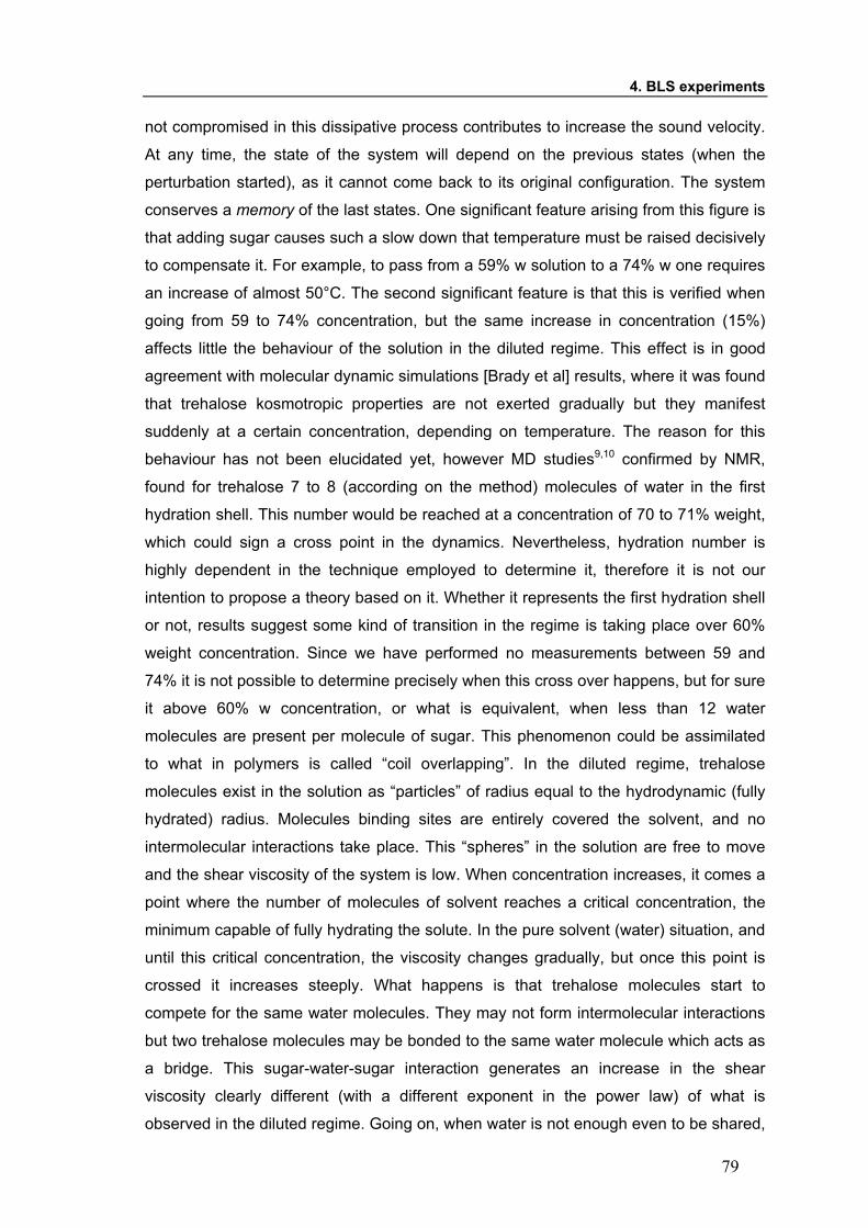
4. BLS experiments
79
not compromised in this dissipative process contributes to increase the sound velocity.
At any time, the state of the system will depend on the previous states (when the
perturbation started), as it cannot come back to its original configuration. The system
conserves a memory of the last states. One significant feature arising from this figure is
that adding sugar causes such a slow down that temperature must be raised decisively
to compensate it. For example, to pass from a 59% w solution to a 74% w one requires
an increase of almost 50°C. The second significant feature is that this is verified when
going from 59 to 74% concentration, but the same increase in concentration (15%)
affects little the behaviour of the solution in the diluted regime. This effect is in good
agreement with molecular dynamic simulations [Brady et al] results, where it was found
that trehalose kosmotropic properties are not exerted gradually but they manifest
suddenly at a certain concentration, depending on temperature. The reason for this
behaviour has not been elucidated yet, however MD studies9,10 confirmed by NMR,
found for trehalose 7 to 8 (according on the method) molecules of water in the first
hydration shell. This number would be reached at a concentration of 70 to 71% weight,
which could sign a cross point in the dynamics. Nevertheless, hydration number is
highly dependent in the technique employed to determine it, therefore it is not our
intention to propose a theory based on it. Whether it represents the first hydration shell
or not, results suggest some kind of transition in the regime is taking place over 60%
weight concentration. Since we have performed no measurements between 59 and
74% it is not possible to determine precisely when this cross over happens, but for sure
it above 60% w concentration, or what is equivalent, when less than 12 water
molecules are present per molecule of sugar. This phenomenon could be assimilated
to what in polymers is called “coil overlapping”. In the diluted regime, trehalose
molecules exist in the solution as “particles” of radius equal to the hydrodynamic (fully
hydrated) radius. Molecules binding sites are entirely covered the solvent, and no
intermolecular interactions take place. This “spheres” in the solution are free to move
and the shear viscosity of the system is low. When concentration increases, it comes a
point where the number of molecules of solvent reaches a critical concentration, the
minimum capable of fully hydrating the solute. In the pure solvent (water) situation, and
until this critical concentration, the viscosity changes gradually, but once this point is
crossed it increases steeply. What happens is that trehalose molecules start to
compete for the same water molecules. They may not form intermolecular interactions
but two trehalose molecules may be bonded to the same water molecule which acts as
a bridge. This sugar-water-sugar interaction generates an increase in the shear
viscosity clearly different (with a different exponent in the power law) of what is
observed in the diluted regime. Going on, when water is not enough even to be shared,
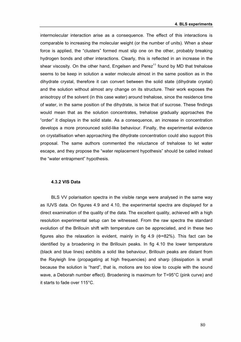
4. BLS experiments
80
intermolecular interaction arise as a consequence. The effect of this interactions is
comparable to increasing the molecular weight (or the number of units). When a shear
force is applied, the “clusters” formed must slip one on the other, probably breaking
hydrogen bonds and other interactions. Clearly, this is reflected in an increase in the
shear viscosity. On the other hand, Engelsen and Perez11 found by MD that trehalose
seems to be keep in solution a water molecule almost in the same position as in the
dihydrate crystal, therefore it can convert between the solid state (dihydrate crystal)
and the solution without almost any change on its structure. Their work exposes the
anisotropy of the solvent (in this case water) around trehalose, since the residence time
of water, in the same position of the dihydrate, is twice that of sucrose. These findings
would mean that as the solution concentrates, trehalose gradually approaches the
“order” it displays in the solid state. As a consequence, an increase in concentration
develops a more pronounced solid-like behaviour. Finally, the experimental evidence
on crystallisation when approaching the dihydrate concentration could also support this
proposal. The same authors commented the reluctance of trehalose to let water
escape, and they propose the “water replacement hypothesis” should be called instead
the “water entrapment” hypothesis.
4.3.2 VIS Data
BLS VV polarisation spectra in the visible range were analysed in the same way
as IUVS data. On figures 4.9 and 4.10, the experimental spectra are displayed for a
direct examination of the quality of the data. The excellent quality, achieved with a high
resolution experimental setup can be witnessed. From the raw spectra the standard
evolution of the Brillouin shift with temperature can be appreciated, and in these two
figures also the relaxation is evident, mainly in fig 4.9 (Φ=82%). This fact can be
identified by a broadening in the Brillouin peaks. In fig 4.10 the lower temperature
(black and blue lines) exhibits a solid like behaviour, Brillouin peaks are distant from
the Rayleigh line (propagating at high frequencies) and sharp (dissipation is small
because the solution is “hard”, that is, motions are too slow to couple with the sound
wave, a Deborah number effect). Broadening is maximum for T=95°C (pink curve) and
it starts to fade over 115°C.

4. BLS experiments
81
-20 -10 0 10 2010-1
100
101
φ=82 %
Inte
nsity
Frequency [GHz]
27.2°C 35°C 42°C 50°C 57°C 65°C 72°C 80°C 87°C 95°C 103°C 113°C
Figure 4.9 – Experimental spectra for a trehalose solution 82% w. Evolution of the Brillouin
peaks with temperature.
-20 -10 0 10 20100
101
102
103
104
105
φ=59 %
Inte
nsity
Frequency [GHz]
40°C 27°C 22°C 17°C 12°C 7°C 2°C -3°C -8°C
Figure 4.10 – Experimental spectra for a trehalose solution 59 % w.
For figure 4.10 this broadening is not so evident. It happens around 17°C (red
curve), so the first and the last curves are sharper, in the case of -8°C getting away as
temperature falls (increasing the shift) and over 40°C the solution approaches the fully
relaxed (liquid like) regime. Classical DHO analysis for these measurements yields the
parameters plotted in figures 4.9 and 4.10.
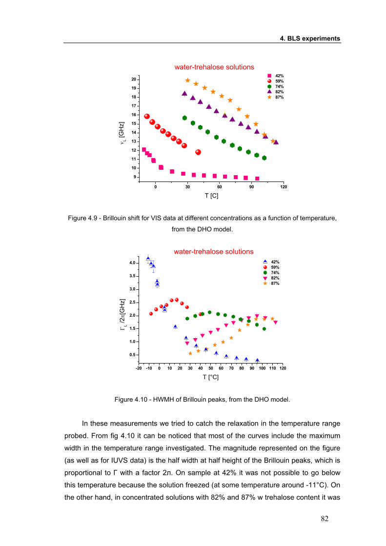
4. BLS experiments
82
0 30 60 90 120
9
10
11
12
13
14
15
16
17
18
19
20 42% 59% 74% 82% 87%
water-trehalose solutions
ν L [GH
z]
T [C]
Figure 4.9 - Brillouin shift for VIS data at different concentrations as a function of temperature,
from the DHO model.
-20 -10 0 10 20 30 40 50 60 70 80 90 100 110 120
0.5
1.0
1.5
2.0
2.5
3.0
3.5
4.0 42% 59% 74% 82% 87%
water-trehalose solutions
ΓL /2
π[G
Hz]
T [°C]
Figure 4.10 - HWMH of Brillouin peaks, from the DHO model.
In these measurements we tried to catch the relaxation in the temperature range
probed. From fig 4.10 it can be noticed that most of the curves include the maximum
width in the temperature range investigated. The magnitude represented on the figure
(as well as for IUVS data) is the half width at half height of the Brillouin peaks, which is
proportional to Γ with a factor 2л. On sample at 42% it was not possible to go below
this temperature because the solution freezed (at some temperature around -11°C). On
the other hand, in concentrated solutions with 82% and 87% w trehalose content it was
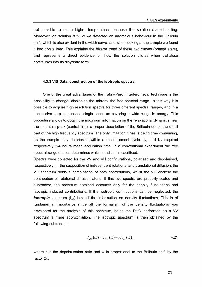
4. BLS experiments
83
not possible to reach higher temperatures because the solution started boiling.
Moreover, on solution 87% w we detected an anomalous behaviour in the Brillouin
shift, which is also evident in the width curve, and when looking at the sample we found
it had crystallised. This explains the bizarre trend of these two curves (orange stars),
and represents a direct evidence on how the solution dilutes when trehalose
crystallises into its dihydrate form.
4.3.3 VIS Data, construction of the isotropic spectra. One of the great advantages of the Fabry-Perot interferometric technique is the
possibility to change, displacing the mirrors, the free spectral range. In this way it is
possible to acquire high resolution spectra for three different spectral ranges, and in a
successive step compose a single spectrum covering a wide range in energy. This
procedure allows to obtain the maximum information on the relaxational dynamics near
the mountain peak (central line), a proper description of the Brillouin doublet and still
part of the high frequency spectrum. The only limitation it has is being time consuming,
as the sample may deteriorate within a measurement cycle. IVV and IVH required
respectively 2-4 hours mean acquisition time. In a conventional experiment the free
spectral range chosen determines which condition is sacrificed.
Spectra were collected for the VV and VH configurations, polarised and depolarised,
respectively. In the supposition of independent rotational and translational diffusion, the
VV spectrum holds a combination of both contributions, whilst the VH enclose the
contribution of rotational diffusion alone. If this two spectra are properly scaled and
subtracted, the spectrum obtained accounts only for the density fluctuations and
Isotropic induced contributions. If the isotropic contributions can be neglected, the
isotropic spectrum (Iρρ) has all the information on density fluctuations. This is of
fundamental importance since all the formalism of the density fluctuations was
developed for the analysis of this spectrum, being the DHO performed on a VV
spectrum a mere approximation. The isotropic spectrum is then obtained by the
following subtraction:
)()()( ωωωρρ VHVV rIII −= , 4.21
where r is the depolarisation ratio and w is proportional to the Brillouin shift by the
factor 2л.
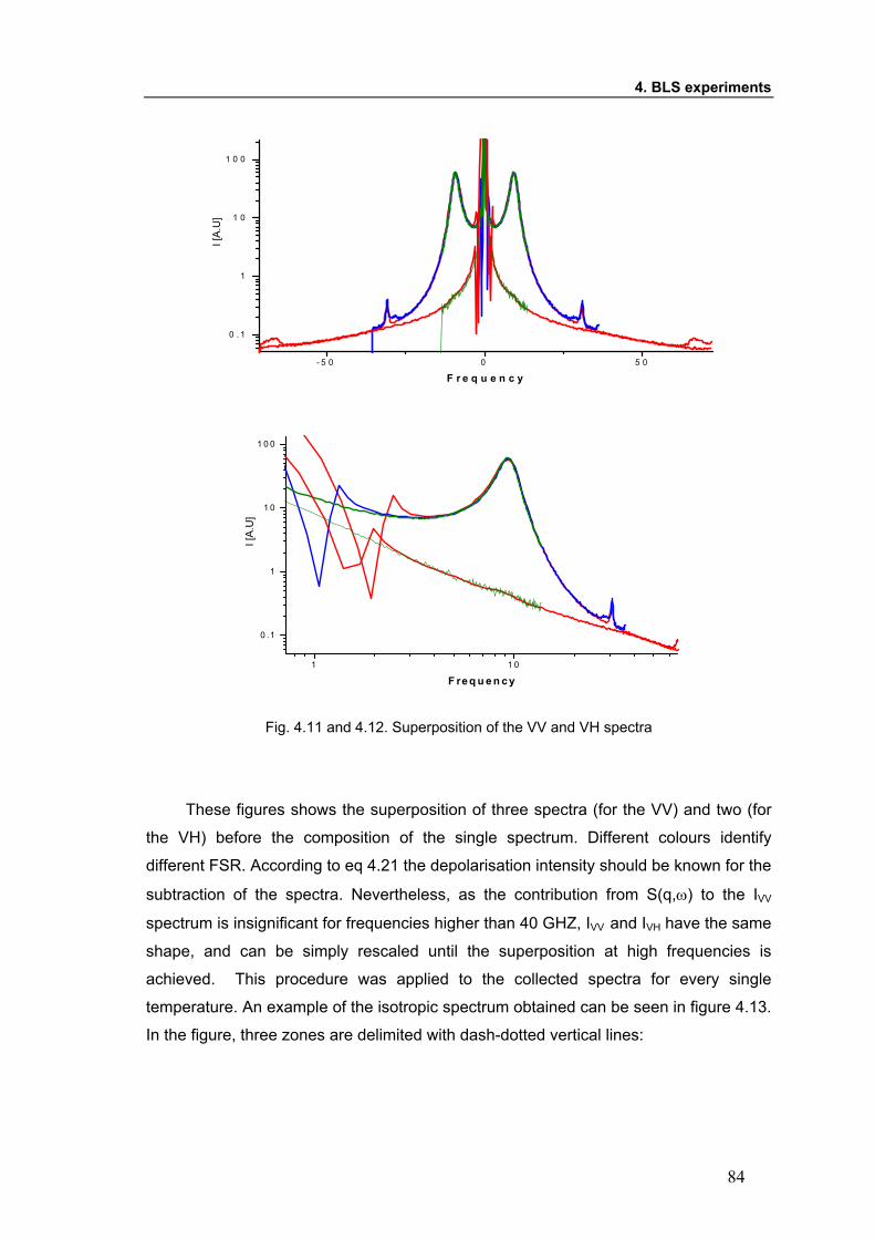
4. BLS experiments
84
- 5 0 0 5 0
0 . 1
1
1 0
1 0 0
I [A.
U]
F r e q u e n c y
1 1 0
0 .1
1
1 0
1 0 0
I [A.
U]
F re q u e n c y
Fig. 4.11 and 4.12. Superposition of the VV and VH spectra
These figures shows the superposition of three spectra (for the VV) and two (for
the VH) before the composition of the single spectrum. Different colours identify
different FSR. According to eq 4.21 the depolarisation intensity should be known for the
subtraction of the spectra. Nevertheless, as the contribution from S(q,ω) to the IVV
spectrum is insignificant for frequencies higher than 40 GHZ, IVV and IVH have the same
shape, and can be simply rescaled until the superposition at high frequencies is
achieved. This procedure was applied to the collected spectra for every single
temperature. An example of the isotropic spectrum obtained can be seen in figure 4.13.
In the figure, three zones are delimited with dash-dotted vertical lines:
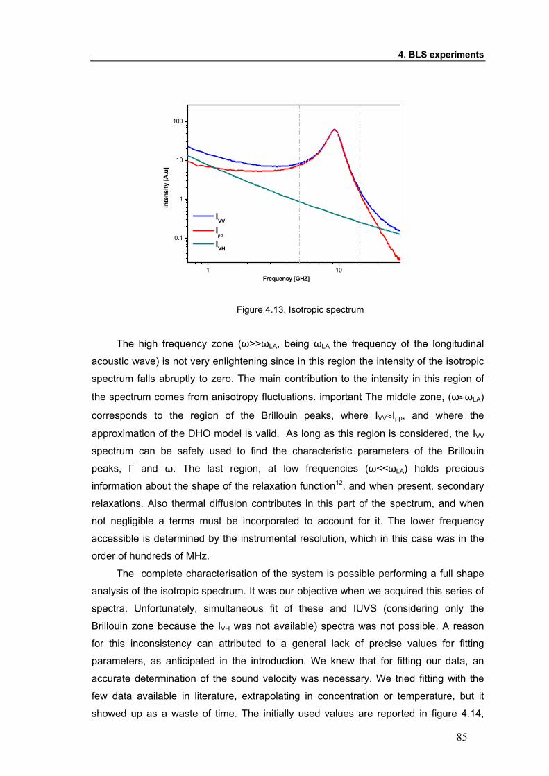
4. BLS experiments
85
1 10
0.1
1
10
100
IVV
Iρρ
IVH
Inte
nsity
[A.u
]
Frequency [GHZ]
Figure 4.13. Isotropic spectrum
The high frequency zone (ω>>ωLA, being ωLA the frequency of the longitudinal
acoustic wave) is not very enlightening since in this region the intensity of the isotropic
spectrum falls abruptly to zero. The main contribution to the intensity in this region of
the spectrum comes from anisotropy fluctuations. important The middle zone, (ω≈ωLA)
corresponds to the region of the Brillouin peaks, where IVV≈Iρρ, and where the
approximation of the DHO model is valid. As long as this region is considered, the IVV
spectrum can be safely used to find the characteristic parameters of the Brillouin
peaks, Γ and ω. The last region, at low frequencies (ω<<ωLA) holds precious
information about the shape of the relaxation function12, and when present, secondary
relaxations. Also thermal diffusion contributes in this part of the spectrum, and when
not negligible a terms must be incorporated to account for it. The lower frequency
accessible is determined by the instrumental resolution, which in this case was in the
order of hundreds of MHz.
The complete characterisation of the system is possible performing a full shape
analysis of the isotropic spectrum. It was our objective when we acquired this series of
spectra. Unfortunately, simultaneous fit of these and IUVS (considering only the
Brillouin zone because the IVH was not available) spectra was not possible. A reason
for this inconsistency can attributed to a general lack of precise values for fitting
parameters, as anticipated in the introduction. We knew that for fitting our data, an
accurate determination of the sound velocity was necessary. We tried fitting with the
few data available in literature, extrapolating in concentration or temperature, but it
showed up as a waste of time. The initially used values are reported in figure 4.14,
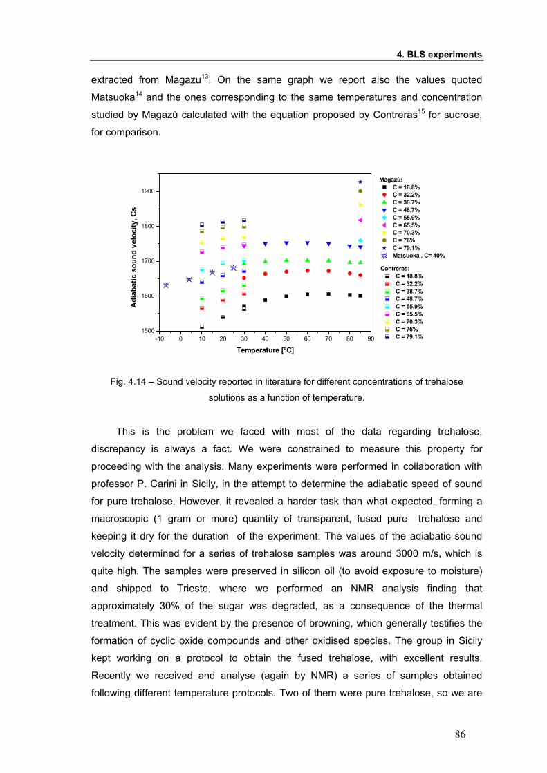
4. BLS experiments
86
extracted from Magazu13. On the same graph we report also the values quoted
Matsuoka14 and the ones corresponding to the same temperatures and concentration
studied by Magazù calculated with the equation proposed by Contreras15 for sucrose,
for comparison.
-10 0 10 20 30 40 50 60 70 80 901500
1600
1700
1800
1900
Magazù: C = 18.8% C = 32.2% C = 38.7% C = 48.7% C = 55.9% C = 65.5% C = 70.3% C = 76% C = 79.1% Matsuoka , C= 40%
Adi
abat
ic s
ound
vel
ocity
, Cs
Temperature [°C]
Contreras: C = 18.8% C = 32.2% C = 38.7% C = 48.7% C = 55.9% C = 65.5% C = 70.3% C = 76% C = 79.1%
Fig. 4.14 – Sound velocity reported in literature for different concentrations of trehalose
solutions as a function of temperature.
This is the problem we faced with most of the data regarding trehalose,
discrepancy is always a fact. We were constrained to measure this property for
proceeding with the analysis. Many experiments were performed in collaboration with
professor P. Carini in Sicily, in the attempt to determine the adiabatic speed of sound
for pure trehalose. However, it revealed a harder task than what expected, forming a
macroscopic (1 gram or more) quantity of transparent, fused pure trehalose and
keeping it dry for the duration of the experiment. The values of the adiabatic sound
velocity determined for a series of trehalose samples was around 3000 m/s, which is
quite high. The samples were preserved in silicon oil (to avoid exposure to moisture)
and shipped to Trieste, where we performed an NMR analysis finding that
approximately 30% of the sugar was degraded, as a consequence of the thermal
treatment. This was evident by the presence of browning, which generally testifies the
formation of cyclic oxide compounds and other oxidised species. The group in Sicily
kept working on a protocol to obtain the fused trehalose, with excellent results.
Recently we received and analyse (again by NMR) a series of samples obtained
following different temperature protocols. Two of them were pure trehalose, so we are
4. BLS experiments
87
optimist that the full shape analysis will be possible soon, but we regret it won’t be for
the time this thesis is presented.
Another way we tried was to measure C∞, the limit of the sound velocity for very
high frequencies. This parameter would be as useful as the adiabatic sound velocity,
as knowing one allows to calculate the other. The main problem is that the available
instruments for this measurement are rare. We submitted a proposal at the ESRF
synchrotron facility but we had no time allocated. Proposals are frequently copious and
the available beamtime is restricted, so we know it is difficult to access this instrument,
but we keep trying.
4.3.4 IUVS and VIS Data
4.3.4.1 Estimation of the activation energy of the relaxation process.
The traditional acoustic analysis yields the parameters Γ and Ω. Under certain
assumptions, they can be used to get, as a good approximation, information about the
characteristic relaxation time τ.
In the formalism of the elastic modulus, from eq. 4.12 it is possible to express the
dynamic structure factor as2:
[ ] [ ]2222 )('')('/
)(''),(ωωρω
ωωMMq
MqS+−
∝ 4.22
where M’ and M’’ are the real and imaginary part of the elastic modulus. Combining this
and eq. 4.18 for γ=1 the following relations are obtained:
2
2
)('q
M BB
ρωω = and 2)(''
qM BB
BΓ
=ρω
ω 4.23; 4.24
so the relaxation can be evenly characterised as a function of M’ and M’’, where
the first one accounts for the propagating processes and the second for the dissipative
ones, showing a peak at 1−= τω corresponding to a maximum in the absorption of the
acoustic energy. In the assumption of a single relaxation (Debye), in the hydrodynamic
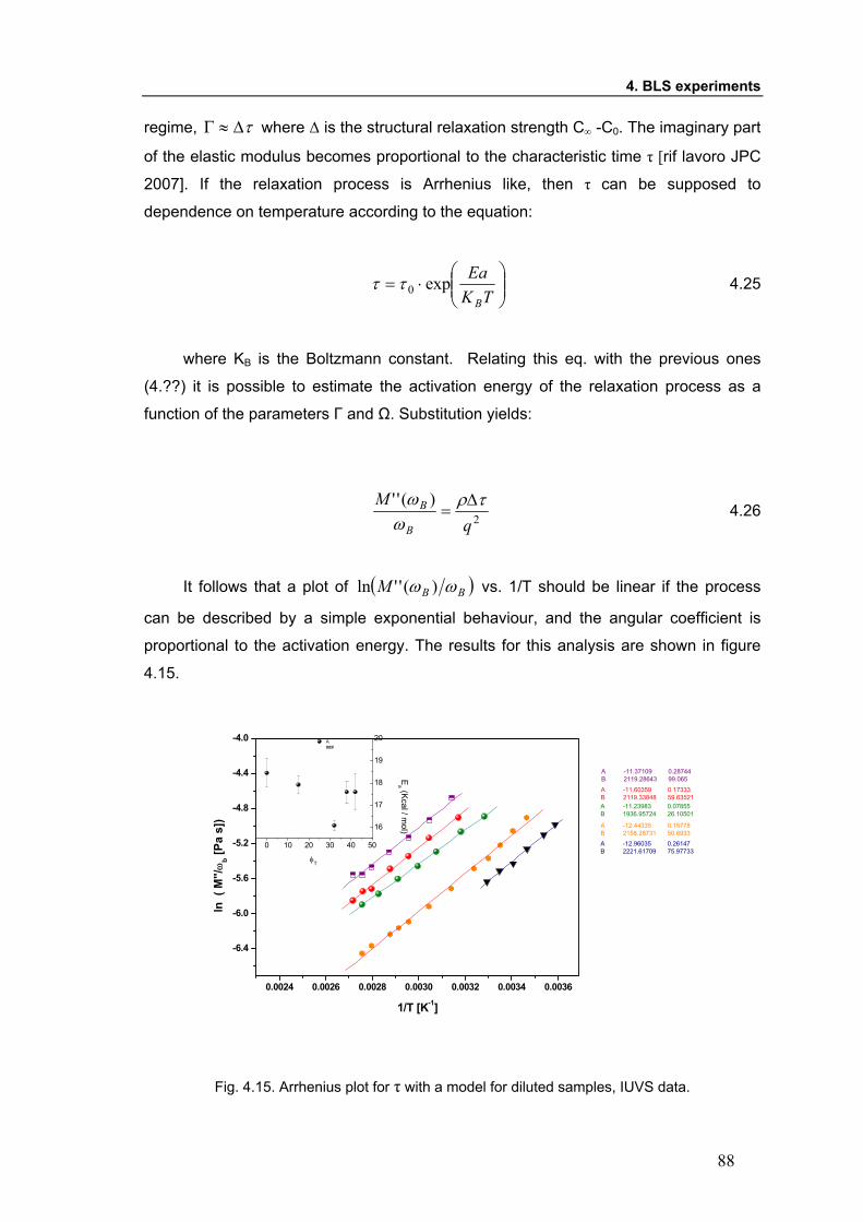
4. BLS experiments
88
regime, τ∆≈Γ where ∆ is the structural relaxation strength C∞ -C0. The imaginary part
of the elastic modulus becomes proportional to the characteristic time τ [rif lavoro JPC
2007]. If the relaxation process is Arrhenius like, then τ can be supposed to
dependence on temperature according to the equation:
⋅=
TKEa
Bexp0ττ 4.25
where KB is the Boltzmann constant. Relating this eq. with the previous ones
(4.??) it is possible to estimate the activation energy of the relaxation process as a
function of the parameters Γ and Ω. Substitution yields:
2)(''
qM
B
B τρω
ω ∆= 4.26
It follows that a plot of ( )BBM ωω )(''ln vs. 1/T should be linear if the process
can be described by a simple exponential behaviour, and the angular coefficient is
proportional to the activation energy. The results for this analysis are shown in figure
4.15.
0.0024 0.0026 0.0028 0.0030 0.0032 0.0034 0.0036
-6.4
-6.0
-5.6
-5.2
-4.8
-4.4
-4.0
A -12.96035 0.26147B 2221.61709 75.97733
A -11.37109 0.28744B 2119.28643 99.065
A -12.44335 0.15778B 2158.28731 50.6933
φT
Ea (K
cal / mol)
A -11.60359 0.17333B 2119.33848 59.63521A -11.23983 0.07855B 1936.95724 26.10501
ln (
M''/
ωb [P
a s]
)
1/T [K-1]
0 10 20 30 40 50
16
17
18
19
20 A ###
Fig. 4.15. Arrhenius plot for τ with a model for diluted samples, IUVS data.

4. BLS experiments
89
The activation energy calculated with this method is in the order of 16±3 KJ/mol,
which is similar to the one found for water16 . This analysis was safe for 1<<ωτ , that is
in the diluted regime, at high temperatures. As our data explore some of the semi
diluted and concentrated regime, a method was needed for evaluating this range. On
the basis of the same hypothesis as before (single relaxation Debye process, γ=1), but
in the framework of the memory function formalism, the relaxation time can be
expressed as follows17
−
Γ= 2
22
11
B
S
B
qCω
τ 4.27
The results of the analysis according to this method can be seen in figure 4.16
(for IUVS data) and 4.17 for VIS spectra. In the latter, two series corresponding to 74%
and 59% of the IUVS data have been included for comparison. It is possible to see that
for low temperatures, linear fitting is appropriate. The activation energy obtained by this
method is in the same order as in the previous case, lower for single IUVS data
(around 12 kJ/mol) and somewhat higher for VIS data (approximately 16 kJ/mol), in
excellent agreement with the first analysis for the diluted regime. What emerges from
this analysis is that even if there may be some degree of uncertainty in the absolute
value of the relaxation time, the trend should not be affected by the assumptions on
the models. In the temperature and concentration ranges where the models were
applied, the system seems to have an Arrhenius like behaviour.
Fig. 4.16. Arrhenius plot for concentrated samples, IUVS data

4. BLS experiments
90
0.0025 0.0030 0.0035 0.0040
1
2
3
4
5
6
60 65 70 75 8012
13
14
15
16
17
BLS 59 % BLS 42%
A -2.43229 0.13664B 1516.43616 43.93488
A -2.72711 0.18307B 1641.87166 55.29682
A -1.72230.06731B 1910.11327 22.59017
A -2.21563 0.19577B 1814.57693 64.9845
A -2.49941 0.15116B 1689.31898 41.88755
BLS 74% BLS 82%IUVS 59% IUVS 74%
IUVS59% Y =-2.85912+1679.27946 X
BLS
Trehalose solutionsComparison of Ea IUVS-BLS
ln (τ
)
1/T[K-1]
ΦT
Fig. 4.17. Arrhenius plot for concentrated solutions, VIS data.
The activation energy found for trehalose-water systems studied by Brillouin light
scattering leads us to conclude that with these techniques we can monitor changes in
the dynamical behaviour of the solutions in terms of formation and breaking of
hydrogen bonds, which is particularly suitable for objectives of our research.
4.3.4.2 Further considerations
Following the line of thought of the first comments about sound dispersion, an
approximate analysis of the curves of Г was performed. As the maximum of the
attenuation should be verified (roughly) at the condition of maximum sensitivity when
1≈ωτ , we wanted to follow the trend in temperature of the relaxation. A Gaussian
curve was simulated on 5 or 6 points (when possible) for every Г around the cusp. In
the most diluted solution (37%) the Gaussian was extrapolated. We displayed the
points calculated as a function of trehalose concentration. The mean error in
temperature should be inferior to 5°C for curves where the peak is evident and
somewhat higher when it was extrapolated. The resulting trend is much like the one of
the glass transition temperature of the solution, but when the difference between peak
temperature and Tg was calculated, we found the curve in the inset of figure 4.18. We
could make a speculative discussion on the divergence in the trend of both

4. BLS experiments
91
30 35 40 45 50 55 60 65 70 75 80 85-120
-100
-80
-60
-40
-20
0
20
40
60
80
100
120
30 60 90
90
100
110
120
130
Peak Temperature from VIS dataPeak temperature from IUVS Tg for the same concentration
Peak
tem
pera
ture
[°C
]
Concentration [Trehalose%w]
T-T
g
temperatures when raising the concentration. T peak and Tg travel parallel for
concentrations below 60%. For superior concentration values the divergence gets more
and more pronounced. This effect suggests that as the solution concentrates, for some
reason (which we will not attempt to explain with so exploratory results) the trend of the
characteristic time of the phenomenon observed with a probe in the Brillouin frequency
range, departs from that determined at 100s, the calorimetric glass transition.
Figure 4.18 – Peak temperature from Г curves Vs calorimetric Tg.
The last step was to evaluate how did the activation energy calculated from our
experiments fit in the overall framework of literature. We report in figure 4.19 the
activation energies reported by De Gusseme et al. 18 for two different β relaxations of
pure trehalose and those provided by Matsuoka et al14 for aqueous solutions of
trehalose from 20 to 50%, obtained by means of dielectric spectroscopy and viscosity.
The interesting element of this comparison is that the activation energy of the alpha
relaxation process reported by Matsuoka seems to evolve in the energy of the beta
relaxation reported by the Gusseme. Moreover, the two different techniques used by
Matsuoka yield two trends that seem to precede De Gusseme’s values for pure
trehalose. Our data do not fit with the rest, probably because of a major sensitivity to
fast motions (water). We stress that these last comments are merely speculative, and
that a further comprehension of the dynamical characteristics of the trehalose-water
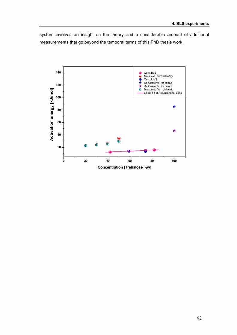
4. BLS experiments
92
0 20 40 60 80 100
20
40
60
80
100
120
140
Ours, BLS Matsuoka, from viscosity Ours, IUVS De Gusseme, for beta 2 De Gusseme, for beta 1 Matsuoka, from dielectric Linear Fit of Activationene_Ean2
Act
ivat
ion
ener
gy [k
J/m
ol]
Concentration [ trehalose %w]
system involves an insight on the theory and a considerable amount of additional
measurements that go beyond the temporal terms of this PhD thesis work.

References for Chapter 4
93
References 1. B.J.Berne and R.Pecora Dynamic Light Scattering. Wiley, New York (1976).
2. Comez, L., Fioretto, D., Scarponi, F. & Monaco, G. Density fluctuations in the intermediate glass-former glycerol: A Brillouin light scattering study. Journal of Chemical Physics 119, 6032-6043 (2003).
3. Zaidi, A. A., Makdisi, Y., Bhatia, K. S. & Abutahun, I. Accurate method for the determination of the refractive index of liquids using a laser. Review of Scientific Instruments 60, 803-805 (1989).
4. Masciovecchio, C. et al. Structural relaxation in liquid water by inelastic UV scattering. Physical Review Letters 92, 255507-1 (2004).
5. Masciovecchio, C., Gessini, A. & Santucci, S. C. Ultraviolet Brillouin scattering as a new tool to investigate disordered systems. Journal of Non-Crystalline Solids 352, 5126-5129 (2006).
6. http://ghost.fisica.unipg.it/. 2008. Ref Type: Generic
7. F.Nizzoli and J.R.Sandercock Dynamical properties of solids. North Holland, Amsterdam (1990).
8. Cummins, H. Z. et al. The liquid-glass transition in sugars: Relaxation dynamics in trehalose. Journal of Non-Crystalline SolidsProceedings of the 5th International Discussion Meeting on Relaxations in Complex Systems, 5th International Discussion Meeting on Relaxations in Complex Systems 352, 4464-4474 (2006).
9. Kawai, H., Sakurai, M., Inoue, Y., Chu?jo?, R. & Kobayashi, S. Hydration of oligosaccharides: Anomalous hydration ability of trehalose. Cryobiology 29, 599-606 (1992).
10. Sakurai, M., Murata, M., Inoue, Y., Hino, A. & Kobayashi, S. Molecular-dynamics study of aqueous solution of trehalose and maltose: Implication for the biological function of trehalose. Bulletin of the Chemical Society of Japan 70, 847-858 (1997).
11. Engelsen, S. B. & Ferez, S. Unique similarity of the asymmetric trehalose solid-state hydration and the diluted aqueous-solution hydration. Journal of Physical Chemistry B 104, 9301-9311 (2000).
12. Fioretto, D. et al. Dynamics of density fluctuations of a glass-forming epoxy resin revealed by Brillouin light scattering. Physical Review E - Statistical Physics, Plasmas, Fluids, and Related Interdisciplinary Topics 59, 1899-1907 (1999).
13. Magazu, S., Migliardo, P., Musolino, A. M. & Sciortino, M. T. -Trehalose-Water Solutions. 1. Hydration Phenomena and Anomalies in the Acoustic Properties. J. Phys. Chem. B 101, 2348-2351 (1997).
14. Matsuoka, T., Okada, T., Murai, K., Koda, S. & Nomura, H. Dynamics and hydration of trehalose and maltose in concentrated solutions. Journal of Molecular Liquids 98-99, 317-327 (2002).

References for Chapter 4
94
15. Contreras, N. I., Fairley, P., McClements, D. J. & Povey, M. J. W. Analysis of the sugar content of fruit juices and drinks using ultrasonic velocity measurements. Int. J. Food Sci. Technol. 27, 515-529 (1992).
16. Monaco, G., Cunsolo, A., Ruocco, G. & Sette, F. Viscoelastic behavior of water in the terahertz-frequency range: an inelastic x-ray scattering study. Phys. Rev. E. Stat. Phys. Plasmas. Fluids Relat Interdiscip. Topics. 60, 5505-5521 (1999).
17. Di Fonzo, S. et al. Concentration-temperature dependencies of structural relaxation time in trehalose-water solutions by brillouin inelastic UV scattering. Journal of Physical Chemistry A 111, 12577-12583 (2007).
18. De Gusseme, A., Carpentier, L., Willart, J. F. & Descamps, M. Molecular mobility in supercooled trehalose. Journal of Physical Chemistry B 107, 10879-10886 (2003).
Conclusions and perspectives
95
This research work discussed some physical features of trehalose and trehalose
water systems that supplement the results of previous studies, both in the field of our
laboratory as well as others. The final aim is to disclose some properties which could
be relevant in bioprotection.
Among the results here presented, the existence of two different “polyamorphic”
forms of trehalose surely adds an additional complexity to the question of its role in
bioprotection. Furthermore, the different dynamic and thermodynamic behaviour of the
amorphous phases A and B can explain, in part, some of the controversial results
reported in literature regarding pure trehalose. As long as experiments (calorimetric,
spectroscopic) are carried out on dynamical properties of trehalose “amorphous phase”
regardless of the existence of these two distinct phases, results will keep on being
discordant. In particular, our ageing experiments led to two different activation energies
for the structural relaxation of the amorphous phases, suggesting that in one of the
glasses molecular mobility is slower than in the other (more homogeneous, compact
structure?). This result may also have a great interest in industrial applications
(pharmaceutical, foods, ...) searching for tailored products and in optimising processes.
As far as the bioprotection is concerned, however, it is necessary to highlight that
whatever the glass formed upon dehydration, the only possible species involved must
derive from moderate temperature processes. According to a previously proposed
mechanism (Sussich 2001) and considering the conditions under which dehydration
occurs in nature, the amorphous trehalose of type A seems to be the one involved.
On the other side, a traditional acoustic analysis of BLS experiments of trehalose-
water mixtures suggest that the overall dynamics of the system slow down with the
increase in trehalose content, which is in qualitative agreement with what so long
reported in literature. However, in the frequency range studied, and with the
approximations considered in the framework of two different models, there are no
evidences of a particular behaviour of water in the presence of trehalose, as suggested
by many studies. The fact that the activation energy of the main relaxation process in
the frequency studied corresponds approximately to that found in pure water lets us
attribute the main relaxation process to the hydrogen bond breaking and formation
during density fluctuations. Nevertheless, a further analysis would validate these
results, since they are based on the assumption of a single Debye relaxation process,
which probably may not be the case, especially for concentrated solutions. The thriving
experiments of Lelong et al. on the dynamics of semi-dilute trehalose confined
solutions, supports the translation of experiments in bulk solutions to the real condition
in organisms, as according to the authors confinement in the dimensions of a cell
should not affect dynamics.
Conclusions and perspectives
96
The attempt to clarify the mechanism of bioprotection is a formidable task in front
of the practical absence of a peculiar behaviour of trehalose solutions, with respect to
other disaccharides, and its “normal behaviour” as a function of increasing
concentration up to about 70% (w/w). The suggestion of a discontinuity on amorphous
mixture properties upon decreasing water content has already been made and involves
the formation of nanocrystalline dihydrate trehalose which evolves into anhydrous TRE
α and amorphous TRE A.
This view would encourage us to continue in the line of our experiments up to
higher concentrations and enlarging the frequency range. In addition, complementary
measurements are necessary for the determination of the shape of the relaxation
distribution function, as with the scarce and contradictory data available in literature it
was not possible to perform a full shape analysis of our experimental spectra.


