
Molecular Magnetic Properties
Workshop on Theoretical Chemistry
Mariapfarr, Salzburg, Austria
February 14–17, 2006
Trygve Helgaker
Department of Chemistry, University of Oslo, Norway
Overview
• The electronic Hamiltonian in an electromagnetic field
• The calculation of molecular magnetic properties
1

Nonrelativistic electronic Hamiltonian in an electromagnetic field
• classical mechanics of particles
– Newtonian mechanics (1687)
– Lagrangian mechanics (1788)
– Hamiltonian mechanics (1833)
• electromagnetic fields
– Maxwell’s equations (1864)
– scalar and vector potentials
– gauge transformations
• spin-free electron in an electromagnetic field
– the Lagrangian and the Hamiltonian of a particle in an electromagnetic field
– the Schrodinger Hamiltonian (1925)
• spinning electron in an electromagnetic field
– the Dirac equation and electron spin (1928)
– the Schrodinger–Pauli Hamiltonian (Pauli, 1927)
2

Classical mechanics
• Matter is described by Newton’s equations:
F (r,v, t) = ma
– the force defines the system and is obtained from experiment
– conservative forces (e.g., gravitational forces) are obtained from potentials:
F (r) = −∇V (r)
• Radiation is described by Maxwell’s equations:
∇ ·E = ρ/ε0 ← Coulomb’s law
∇ ×B− ε0µ0 ∂E/∂t = µ0J ← Ampere’s law
∇ ·B = 0
∇ ×E + ∂B/∂t = 0 ← Faraday’s law of induction
• The interaction between matter and radiation is described by the Lorentz force:
F (r,v) = z (E + v×B)
3

Lagrangian mechanics: the principle of least action
• For a system of n degrees of freedom, there are
– n generalized coordinates qi in configuration space
– n generalized velocities qi
• The principle of least action (Hamilton’s principle):
For each system, there exists a Lagrangian L(qi, qi, t) such that the action
integral
S =
Z t2
t1
L(qi, qi, t) dt
assumes an extremum along the trajectory in configuration space taken by
the system.
t1 t2
qiHt1L
qiHt2L
4

Lagrange’s equations
• From the principle of least action, we obtain
δS = δ
Z t2
t1
L(qi, qi, t) dt =
Z t2
t1
„∂L
∂qi
δqi +∂L
∂qi
δqi
«
dt
=
Z t2
t1
»∂L
∂qi
δqi −
„d
dt
∂L
∂qi
«
δqi
–
dt = 0
• We conclude that the Lagrangian satisfies the following second-order differential
equations (one for each degree of freedom):
ddt
∂L∂qi
=∂L∂qi
← Lagrange’s equations of motion
– the Lagrangian defines the system and is determined so that it reproduces the
equations of motion consistent with experiment.
– Lagrange’s equations preserve their form in any coordinate system.
• A more general formulation than the Newtonian one:
– unified description of matter and fields (Newton’s and Maxwell’s equations)
– springboard for quantum mechanics
5

Arbitrariness of the Lagrangian and gauge transformations
• The scalar Lagrangian is not uniquely defined.
• Assume that the Lagrangian L(q, q, t) satisfies the equations:
d
dt
∂L
∂q=
∂L
∂q.
• Consider now the following transformed Lagrangian where the arbitrary gauge
function f (q, t) is independent of the velocity q:
L′ (q, q, t) = L (q, q, t) +d
dtf (q, t).
• The new Lagrangian satisfies the same equations of motion as the old one:
d
dt
∂L′
∂q=
d
dt
∂L
∂q+
d
dt
∂
∂q
„∂f
∂qq +
∂f
∂t
«
=∂L
∂q+
d
dt
∂f
∂q=
∂
∂q
„
L +d
dtf
«
=∂L′
∂q.
• This is an example of a gauge transformation.
6

Conservative systems
• The Lagrangian of a particle in a conservative field may be written as
L = T (q, q)| z
kinetic energy
− V (q)| z
potential energy
• The Lagrangian is thus easily set up for any conservative system, in any
convenient coordinate system.
• Example: Assuming a Cartesian coordinate system
L =1
2mv2 − V (r) ,
we find that Lagrange’s equations immediately reduce to Newton’s equations:
d
dt
∂L
∂v=
∂L
∂r⇒
d
dtmv = −∇V (r) ⇒ ma = F.
• For particles in a (nonconservative) electromagnetic field, the Lagrangian can be
cast in similar but slightly different form as discussed later.
7

The energy function
• In Lagrangian mechanics, the energy function is defined as:
h (q, q, t) =∂L
∂qq − L (q, q, t) .
• Assume a conservative Cartesian system with Lagrangian L = 12mv2 − V (r):
h =∂L
∂vv− L =
∂T
∂vv − (T − V ) = 2T − T + V = T + V = total energy
– More generally, h is equal to the total energy if T (q) is quadratic in q and
V (q) is independent of q.
• The energy function h is conserved if L does not depend explicitly on time:
dh
dt= −
∂L
∂t
– Proof:
dh
dt=
d
dt
„∂L
«
−dL
dt
=
»„d
dt
∂L
∂q
«
q +∂L
–
−
»∂L
∂qq +
∂L
∂qq +
∂L
∂t
–
= −∂L
∂t
8

Generalized momentum
• The generalized momentum pi conjugate to the generalized coordinate qi is
defined as
pi =∂L∂qi
← generalized momentum
• For a conservative system in Cartesian coordinates L = 12mv2 − V (r),
the conjugate momentum corresponds to the linear momentum:
p =∂L
∂v=
∂T
∂v=
1
2m
∂v2
∂v= mv ← linear momentum
• The momentum conjugate to a coordinate that does not occur in the Lagrangian
is conserved:
dpi
dt=
d
dt
∂L
∂qi
=∂L
∂qi
= 0 ← if L is independent of qi
– such coordinates are said to be cyclic
• Compare: h is conserved if L does not depend explicitly on t,
pi is conserved if L does not depend explicitly on qi
9
Hamiltonian mechanics
• For a system of n degrees of freedom, there are n second-order differential
equations (Lagrange’s equations):
d
dt
∂L
∂qi
=∂L
∂qi
• The motion is completely specified by the initial values of the n coordinates and
the n velocities.
• In this sense, we may view qi and qi as 2n independent variables.
• Alternatively, let us treat qi and pi as 2n independent variables:
qi, qi → qi, pi
• Possible advantages of such a scheme:
– first-order equations
– better suited to cyclic coordinates
10
The Hamiltonian
• The differential of the Lagrangian L (q, q, t) is given by
dL (q, q, t) =∂L
∂qdq +
∂L
∂qdq +
∂L
∂tdt = pdq + p dq +
∂L
∂tdt
• We now introduce the Hamiltonian, whose differential should be given by:
dH (q, p, t) =∂H
∂qdq +
∂H
∂pdp +
∂H
∂tdt. (1)
• The Legendre transformation
H = pq − L ← the Hamiltonian function
gives the required differential:
dH = (pdq + q dp)− (p dq + pdq +∂L
∂tdt) = −pdq + q dp−
∂L
∂tdt. (2)
• A comparison of (1) and (2) yields
∂H∂q
= −p, ∂H∂p
= q ← Hamilton’s equations
11

Prescription for setting up the Hamiltonian
1. Choose n generalized coordinates qi.
2. Set up the Lagrangian L (qi, qi, t) such that
d
dt
∂L
∂qi
=∂L
∂qi
(1)
reproduces the equations of motion.
3. Introduce the conjugate momenta
pi =∂L
∂qi
. (2)
4. Construct the Hamiltonian
H =X
i
piqi − L (qi, qi, t) (3)
and invert (2) to express the Hamiltonian H (qi, pi) in terms of qi and pi.
5. Write down Hamilton’s equations of motion:
qi =∂H
∂pi
, pi = −∂H
∂qi
. (4)
12

Comparison of Lagrangian and Hamiltonian mechanics
Lagrangian mechanics Hamiltonian mechanics
n second-order equations: 2n first-order equations:ddt
∂L∂qi
= ∂L∂qi
qi = ∂H∂pi
, pi = − ∂H∂qi
qi are the primary variables in
configuration space,
qi secondary variables
qi and pi are independent variables in
phase space, connected only by the
equations of motion
the state of the system is determined
when the variables (qi, qi) are known at
a given time t
the state of the system is defined by a
point (qi, pi) in phase space, moving on
a trajectory that satisfies Hamilton’s
equations of motion
13
Poisson brackets
• The Poisson bracket of two dynamical variables A (q, p, t) and B (q, p, t) is defined
as
[A, B] =X
i
„∂A
∂qi
∂B
∂pi
−∂B
∂qi
∂A
∂pi
«
– the fundamental Poisson brackets among conjugate coordinates and momenta:
[qi, qj ] = 0, [pi, pj ] = 0, [qi, pj ] = δij
• The total time derivatives are given by
dA
dt=
∂A
∂qq +
∂A
∂pp +
∂A
∂t=
∂A
∂q
∂H
∂p−
∂A
∂p
∂H
∂q+
∂A
∂t,
and may therefore be expressed compactly as
dA
dt= [A, H] +
∂A
∂t.
– important special cases:
q = [q, H] , p = [p, H] ,dH
dt=
∂H
∂t
14
Quantization of a particle in conservative force field
• The Hamiltonian formulation is more general than the Newtonian formulation:
– it is invariant to coordinate transformations
– it provides a uniform description of matter and radiation
– it constitutes the springboard to quantum mechanics
• The Hamiltonian function (the total energy) of a particle in a conservative force field:
H(q, p) =p2
2m+ V (q)
• Standard rule for quantization (in Cartesian coordinates):
– carry out the substitutions
p→ −ih∇, H → ih∂
∂t
– multiply the resulting expression by the wave function Ψ(q) from the right:
ih∂Ψ(q)
∂t=
»
−h2
2m∇2 + V (q)
–
Ψ(q)
• This approach is sufficient for a treatment of electrons in an electrostatic field.
• It is insufficient for nonconservative systems—that is, for systems in a general
electromagnetic field.
15

Review: Hamiltonian mechanics
• In classical Hamiltonian mechanics, a system of particles is described in terms their
positions qi and conjugate momenta pi.
• For each such system, there exists a scalar Hamiltonian function H(qi, pi) such that the
classical equations of motion are given by:
qi =∂H
∂pi
, pi = −∂H
∂qi
(Hamilton’s equations of motion)
• Example: a single particle of mass m in a conservative force field F (q)
– the Hamiltonian function is constructed from a scalar potential:
H(q, p) =p2
2m+ V (q), F (q) = −
∂V (q)
∂q
– Hamilton’s equations are equivalent to Newton’s equations:
q =∂H(q,p)
∂p= p
m
p = −∂H(q,p)
∂q= −
∂V (q)∂q
9=
;⇒ mq = F (q) (Newton’s equations of motion)
• Whereas Newton’s equations of motion are second-order differential equations,
Hamilton’s equations are first-order.
• We must now generalize this approach to particles in an electromagnetic field!
16

The Lorentz force and Maxwell’s equations
• In the presence of an electric field E and a magnetic field (magnetic induction) B,
a classical particle of charge z experiences the Lorentz force:
F = z (E + v ×B)
– since this force depends on the velocity v of the particle, it is not conservative
• The electric and magnetic fields E and B satisfy Maxwell’s equations (1861–1868):
∇ · E = ρ/ε0 ← Coulomb’s law
∇×B− ε0µ0 ∂E/∂t = µ0J ← Ampere’s law with Maxwell’s correction
∇ ·B = 0
∇×E + ∂B/∂t = 0 ← Faraday’s law of induction
– when the charge and current densities ρ(r, t) and J(r, t) are known,
Maxwell’s equations can be solved for E(r, t) and B(r, t)
– on the other hand, since the charges (particles) are driven by the Lorentz force,
ρ(r, t) and J(r, t) are functions of E(r, t) and B(r, t)
• In the following, we shall consider the motion of particles in a given (fixed)
electromagnetic field.
17

Scalar and vector potentials
• The second, homogeneous pair of Maxwell’s equations involve only E and B:
∇ ·B = 0 (1)
∇×E +∂B
∂t= 0 (2)
1. Equation (1) is satisfied by introducing the vector potential A:
∇ ·B = 0 ⇒ B = ∇×A ← vector potential (3)
2. Inserting Eq. (3) in Eq. (2) and introducing a scalar potential φ, we obtain
∇×
„
E +∂A
∂t
«
= 0 ⇒ E +∂A
∂t= −∇φ ← scalar potential
• The second pair of Maxwell’s equations are thus automatically satisfied by writing
E = −∇φ−∂A
∂tB = ∇×A
• The potentials (φ,A) contain four rather than six components as in (E,B).
• They are obtained by solving the first, inhomogeneous pair of Maxwell’s equations,
which contains ρ and J.
18

Particle in an electromagnetic field
• For a particle in an electromagnetic field, we must set up a Lagrangian such that
d
dt
∂L
∂qi
=∂L
∂qi
reduces to Newton’s equations with the Lorentz force
F = z (E + v ×B) , E = −∇φ−∂A
∂t, B = ∇×A
• This is not a conservative system, for which
L = T − V, Fi = −∂V
∂qi
• Rather, it belongs to a broader class of systems, for which
L = T − U, Fi = −∂U
∂qi
+d
dt
„∂U
∂qi
«
• For a particle subject to the Lorentz force, the generalized potential is given by
U = z (φ− v ·A) ← velocity-dependent potential
and the Lagrangian becomes
L = T − z (φ− v ·A) ← particle in an electromagnetic field
19

Conjugate momentum in an electromagnetic field
• We recall that, for a conservative system described by Lagrangian of the form
L (q, q) = T (q)− V (q) ,
the conjugate momentum in Cartesian coordinates
p =∂L
∂v=
∂T
∂v= mv ≡ π
is equal to the linear (kinetic) momentum π:
p = π ← particle in a conservative field
• By contrast, for a nonconservative system described by Lagrangian
L (q, q) = T (q)− U (q, q) ,
the conjugate and kinetic momenta are no longer the same.
• In particular, for a particle in an electromagnetic field
L = T − z (φ− v ·A)
we obtain
p =∂L
∂v=
∂T
∂v+ zA ⇒ p = π + zA ← particle in an electromagnetic field
20

The Hamiltonian in an electromagnetic field
• We recall that, for a conservative system with Lagrangian
L = T (q)− V (q) ,
where T (q) is quadratic in q, the Hamiltonian is given by
H = T (q) + V (q) .
• Let us now consider the nonconservative system consisting of a particle in a field
L = T (q)− U (q, q) =1
2mv2 − z (φ− v ·A) .
• From the conjugate momentum
p = mv + zA,
we obtain the Hamiltonian
H = p · v − L =`mv2 + zv ·A
´−
„1
2mv2 − zφ + zv ·A
«
=1
2mv2 + zφ = T + zφ.
• Expressed in canonical coordinates, the Hamiltonian now becomes:
H = T + zφ = (p−zA)·(p−zA)2m
+ zφ
– note: H = T + U + zv ·A 6= T + U
21

Gauge transformations
• The scalar and vector potentials φ and A are not unique.
• Consider the following transformation of the potentials:
φ′ = φ− ∂f∂t
A′ = A + ∇f
9=
;f = f(q, t) ← gauge function of position and time
• This gauge transformation of the potentials does not affect the physical fields:
E′ = −∇φ′ −∂A′
∂t= −∇φ + ∇
∂f
∂t−
∂A
∂t−
∂∇f
∂t= E
B′ = ∇× (A + ∇f) = B + ∇×∇f = B
• We are free to choose f(q, t) so as to make φ and A satisfy additional conditions.
• In the Coulomb gauge, the gauge function is chosen such that the vector potential
becomes divergenceless:
∇ ·A = 0 ← Coulomb gauge
• Note: Gauge transformations induce the following transformations:
L′ = L + zdf
dt, p′ = p + z∇f, H′ = H − z
∂f
∂t, T ′ = T
– However, the equations of motion are unaffected!
22

Quantization of a particle in an electromagnetic field
• We have now constructed a Hamiltonian function such that Hamilton’s equations are
equivalent to Newton’s equation with the Lorentz force:
qi =∂H
∂pi
& pi = −∂H
∂qi
⇔ ma = z (E + v ×B)
• To this end, we introduced scalar and vector potentials φ and A such that
E = −∇φ−∂A
∂t, B = ∇×A
• In terms of these potentials, the classical Hamiltonian function takes the form
H =π2
2m+ zφ, π = p− zA ← kinetic momentum
• Quantization is now accomplished in the usual manner, by the substitutions
p→ −ih∇, H → ih∂
∂t
• This results in the following time-dependent Schrodinger equation for a particle in an
electromagnetic field:
ih∂Ψ
∂t=
1
2m(−ih∇− zA) · (−ih∇− zA)Ψ + zφ Ψ
23
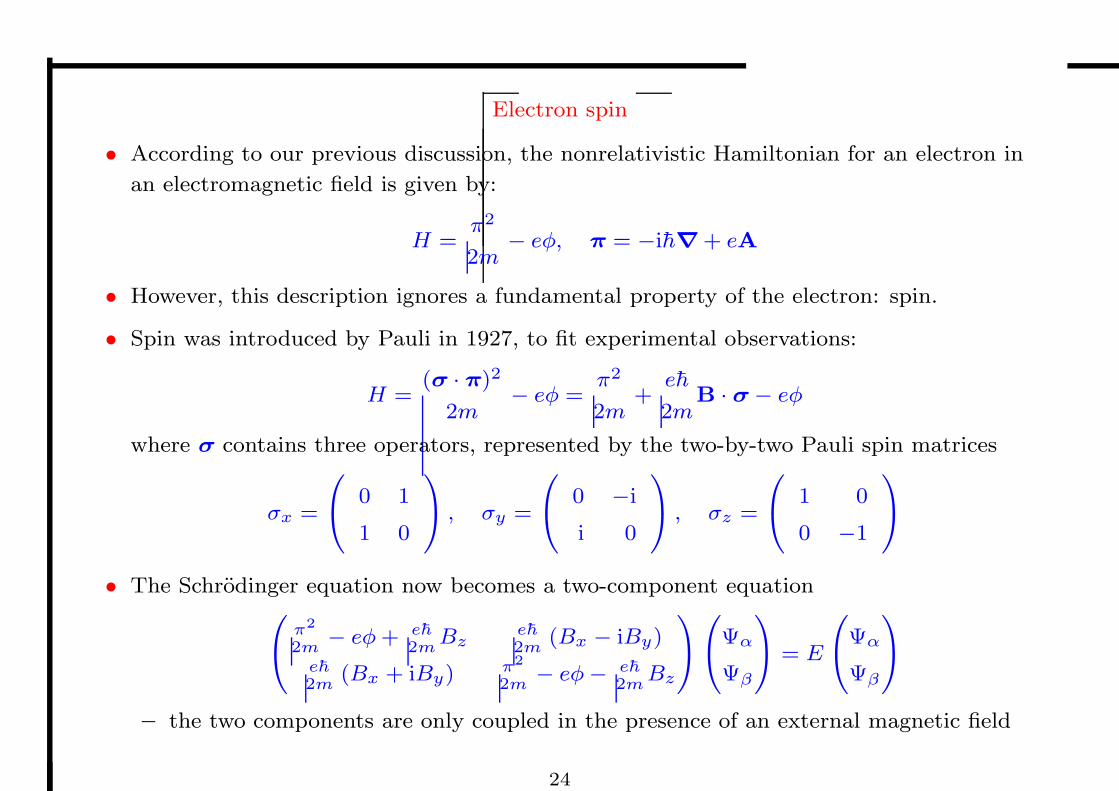
Electron spin
• According to our previous discussion, the nonrelativistic Hamiltonian for an electron in
an electromagnetic field is given by:
H =π2
2m− eφ, π = −ih∇ + eA
• However, this description ignores a fundamental property of the electron: spin.
• Spin was introduced by Pauli in 1927, to fit experimental observations:
H =(σ · π)2
2m− eφ =
π2
2m+
eh
2mB · σ− eφ
where σ contains three operators, represented by the two-by-two Pauli spin matrices
σx =
0
@0 1
1 0
1
A , σy =
0
@0 −i
i 0
1
A , σz =
0
@1 0
0 −1
1
A
• The Schrodinger equation now becomes a two-component equation0
@
π2
2m− eφ + eh
2mBz
eh2m
(Bx − iBy)
eh2m
(Bx + iBy) π2
2m− eφ− eh
2mBz
1
A
0
@Ψα
Ψβ
1
A = E
0
@Ψα
Ψβ
1
A
– the two components are only coupled in the presence of an external magnetic field
24

Spin and relativity
• The introduction of spin by Pauli in 1927 may appear somewhat ad hoc.
• By contrast, spin arises naturally from Dirac’s relativistic treatment in 1928.
– is spin is a relativistic effect?
• However, reduction of Dirac’s equation to nonrelativistic form yields the Hamiltonian
H =(σ · π)2
2m− eφ 6=
π2
2m− eφ
– spin is therefore not a relativistic property of the electron
• Indeed, it is possible to take the factorized form
H =(σ · π)2
2m− eφ
as the starting point for a nonrelativistic treatment, with unspecified operators σ.
• All algebraic properties of σ then follow from the requirement (σ · p)2 = p2:
[σi, σj ]+ = δij , [σi, σj ] = 2ǫijkσk
– these operators are represented by the two-by-two Pauli spin matrices
• We interpret σ by associating an intrinsic angular momentum (spin) with the electron:
s = hσ/2
25

Classical relativistic Hamiltonian
• Hamiltonian for an electron in an electromagnetic field
H =q
m2c4 + c2(p + eA)2 − eφ
• Hamilton’s equations give us
r =∂H
∂p⇒ p = π− eA ← conjugate momentum
p = −∂H
∂r⇒ π = −e(E + v ×B) ← Lorentz force
where the relativistic kinetic momentum is given by
π =mv
p1− v2/c2
← Lorentz factor × nonrelativistic momentum
• Relationship to nonrelativistic mechanics
p
m2c4 + c2π2 = mc2 +π2
2m+O
ˆ(v/c)2
˜
π = mv +Oˆ(v/c)2
˜
– the nonrelativistic limit is obtained as (v/c)2 → 0
26

Linearization of Hamiltonian
• The Hamiltonian is given by
H = cp
π2 + m2c2 − eφ
but we would like time and space coordinates to appear symmetrically in the equation
ih∂Ψ
∂t= HΨ
• Following Dirac, we write
π2 + m2c2 = (αxπx + αyπy + αzπz + α0mc)2
• To determine the αi, we note that
(αxπx + αyπy + · · · )2 = α2xπ2
x + α2yπ2
y + (αxαy + αyαx) πxπy + · · · = π2x + π2
y · · ·
if the αi operators anticommute
α2x = α2
y = 1
αxαy + αyαx = 0
9=
;⇒ [αi, αj ]+ = 2δij
• The Hamiltonian may now be written as
HD = cα · π + βmc2 − eφ, α = [αx, αy , αz ] , β = α0
27

The Dirac equation
• In matrix representation, the anticommuting operators αi are represented by four 4× 4
matrices
αi =
0
@0 σi
σi 0
1
A , β =
0
@I 0
0 −I
1
A ,
where I is the 2× 2 unit matrix and the σi are the usual Pauli spin matrices:
σx =
0
@0 1
1 0
1
A , σy =
0
@0 −i
i 0
1
A , σz =
0
@1 0
0 −1
1
A
• In this representation, the Dirac equation
ih∂Ψ
∂t=
`cα · π + βmc2 − eφ
´Ψ
therefore has a four-component solution:
ih
0
BBBBB@
∂Ψ1∂t
∂Ψ2∂t
∂Ψ3∂t
∂Ψ4∂t
1
CCCCCA
=
0
BBBBB@
mc2 − eφ 0 cπz c(πx − iπy)
0 mc2 − eφ c(πx + iπy) −cπz
cπz c(πx − iπy) −mc2 − eφ 0
c(πx + iπy) −cπz 0 −mc2 − eφ
1
CCCCCA
0
BBBBB@
Ψ1
Ψ2
Ψ3
Ψ4
1
CCCCCA
• Positive solutions are associated with electrons (α and β spin), negative with positrons.
28

The Levy-Leblond equation
• The time-independent Dirac equation may be written in the form:0
@−eφ cσ · π
cσ · π −2mc2 − eφ
1
A
0
@ϕ
χ
1
A =`E −mc2
´
0
@ϕ
χ
1
A .
• Introducing the scaled energy and scaled small component
E′ = E −mc2, χ′ = cχ,
and rearranging, we obtain an equation where c occurs only as c−2:0
@−eφ σ · π
σ · π −2m− c−2eφ
1
A
0
@ϕ
χ′
1
A = E′
0
@ϕ
c−2χ′
1
A .
• Letting c→∞, we obtain the Levy-Leblond equation:0
@−eφ σ · π
σ · π −2m
1
A
0
@ϕ
χ′
1
A = E′
0
@ϕ
0
1
A .
• This is the nonrelativistic limit of the Dirac equation—a useful zero-order equation for
relativistic perturbation theory.
29

The Schrodinger equation
• The Levy-Leblond equation is given by (dropping primes):0
@−eφ σ · π
σ · π −2m
1
A
0
@ϕ
χ
1
A = E
0
@ϕ
0
1
A .
• Solving the second equation for the small component χ
χ =1
2mσ · πϕ
and substituting the result into the first equation, we obtain»
1
2m(σ · π) (σ · π)− eφ
–
ϕ = Eϕ
• Finally, invoking the identity
(σ · u) (σ · v) = u · v + iσ · u× v
we arrive at the two-component Schrodinger equation:»
1
2mπ2 +
1
2miσ · π×π− eφ
–
ϕ = Eϕ
• In the absence of a vector potential, the second term vanishes:
A = 0 ⇒ π×π = p× p = 0
30

Expansion of the kinetic momentum
• Assuming the Coulomb gauge ∇ ·A = 0, we obtain
π2Ψ = (p + eA) · (p + eA)Ψ
= p2Ψ + ep ·AΨ + eA · pΨ + e2A2Ψ
= p2Ψ + e(p ·A)Ψ + 2eA · pΨ + e2A2Ψ
=`p2 + 2eA · p + e2A2
´Ψ
• Recalling the relation ∇×A = B, we obtain
(π× π) Ψ = (p + eA)× (p + eA) Ψ
= ep×AΨ + eA× pΨ
= e (p×A) Ψ + e (pΨ)×A + eA× pΨ
= −ihe (∇×A)Ψ = −iheBΨ
• In the Coulomb gauge, the kinetic energy operator is therefore given by:
T =1
2mπ2 +
1
2miσ · π× π =
1
2mp2 +
e
mA · p +
e
mB · s +
e2
2mA2
where we have used hσ = 2s.
31

Electron spin
• The Dirac Hamiltonian does not commute with the orbital angular momentum operator
but rather with the operator
l +h
2σ
• We therefore assign to the electron an intrinsic spin angular momentum
s =h
2σ
• Likewise, we interpret the Zeeman term by assigning to the electron a magnetic moment
µBσ ·B = −m ·B, µB =eh
2m
where we have introduced is the anomalous spin magnetic moment:
m = −2µBs
• From quantum electrodynamics, one finds that the true spin magnetic moment differs
slightly from that given by Dirac’s theory:
m = −gµBs, g ≈ 2.002
32
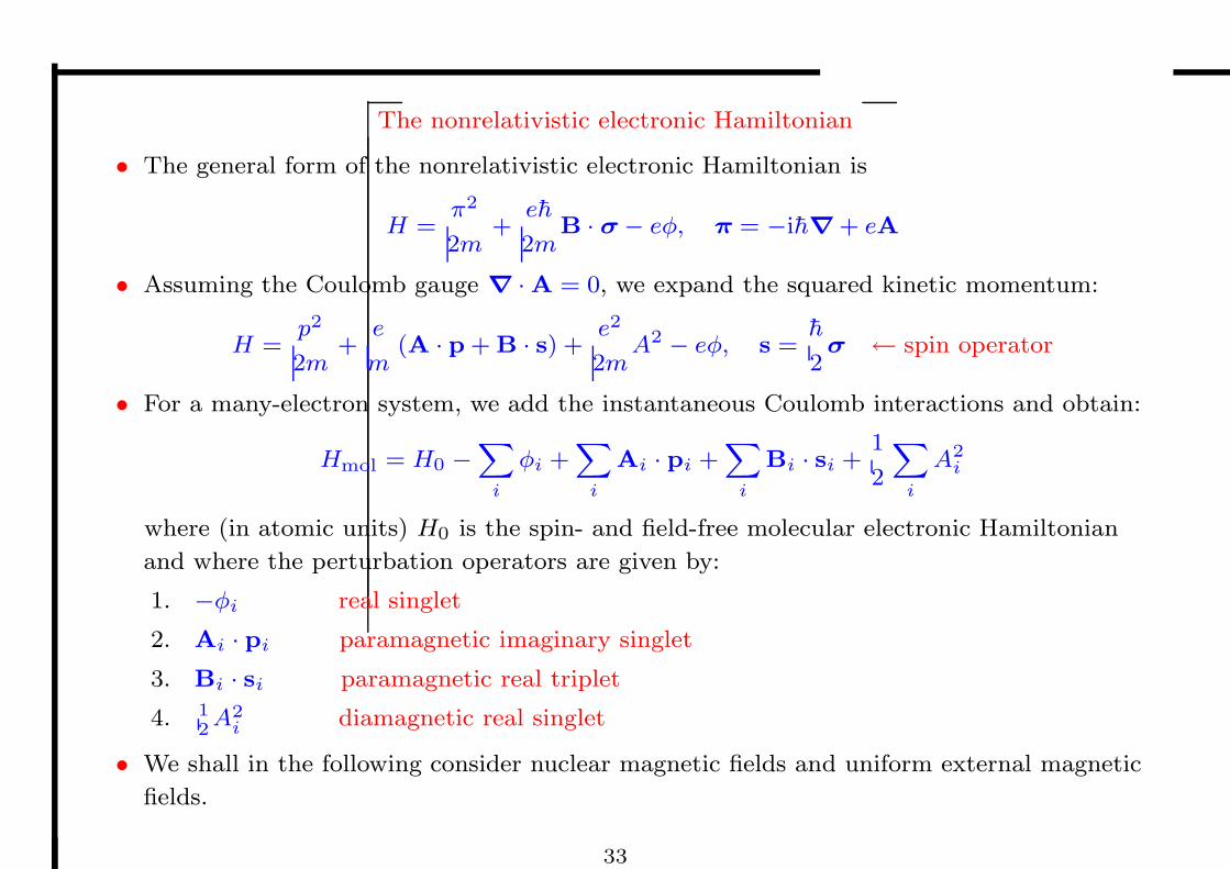
The nonrelativistic electronic Hamiltonian
• The general form of the nonrelativistic electronic Hamiltonian is
H =π2
2m+
eh
2mB · σ− eφ, π = −ih∇ + eA
• Assuming the Coulomb gauge ∇ ·A = 0, we expand the squared kinetic momentum:
H =p2
2m+
e
m(A · p + B · s) +
e2
2mA2 − eφ, s =
h
2σ ← spin operator
• For a many-electron system, we add the instantaneous Coulomb interactions and obtain:
Hmol = H0 −X
i
φi +X
i
Ai · pi +X
i
Bi · si +1
2
X
i
A2i
where (in atomic units) H0 is the spin- and field-free molecular electronic Hamiltonian
and where the perturbation operators are given by:
1. −φi real singlet
2. Ai · pi paramagnetic imaginary singlet
3. Bi · si paramagnetic real triplet
4. 12A2
i diamagnetic real singlet
• We shall in the following consider nuclear magnetic fields and uniform external magnetic
fields.
33

Uniform static electric and magnetic fields
• The scalar and vector potentials of the uniform (static) fields E and B are given by:
E = −∇φ(r, t)−∂A(r,t)
∂t= const
B = ∇×A(r, t) = const
9=
;⇒
8<
:
φ(r) = −E · r
A(r) = 12B× r
• Interaction with the electrostatic field:
−X
i
φ(ri) = E ·X
i
ri = −E · de, de = −X
i
ri ← electric dipole operator
• Orbital paramagnetic interaction with the magnetostatic field:X
i
A · pi = 12
X
i
B× ri · pi = 12B · L, L =
X
i
ri × pi ← orbital ang. mom. op.
• Spin paramagnetic interaction with the magnetostatic field:X
i
B · si = B · S, S =X
i
si ← spin ang. mom. op.
• Total paramagnetic interaction with a uniform magnetic field:
Hz = −B · dm, dm = −1
2(L + 2S) ← Zeeman interaction
34
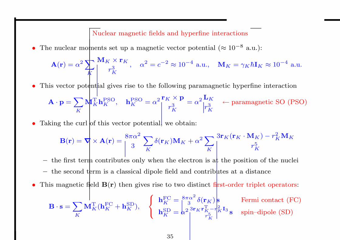
Nuclear magnetic fields and hyperfine interactions
• The nuclear moments set up a magnetic vector potential (≈ 10−8 a.u.):
A(r) = α2X
K
MK × rK
r3K
, α2 = c−2 ≈ 10−4 a.u., MK = γK hIK ≈ 10−4 a.u.
• This vector potential gives rise to the following paramagnetic hyperfine interaction
A · p =X
K
MTKhPSO
K , hPSOK = α2 rK × p
r3K
= α2 LK
r3K
← paramagnetic SO (PSO)
• Taking the curl of this vector potential, we obtain:
B(r) = ∇×A(r) =8πα2
3
X
K
δ(rK)MK + α2X
K
3rK(rK ·MK)− r2KMK
r5K
– the first term contributes only when the electron is at the position of the nuclei
– the second term is a classical dipole field and contributes at a distance
• This magnetic field B(r) then gives rise to two distinct first-order triplet operators:
B · s =X
K
MTK(hFC
K + hSDK ),
8<
:
hFCK = 8πα2
3δ(rK) s Fermi contact (FC)
hSDK = α2 3rKr
TK
−r2K
I3
r5K
s spin–dipole (SD)
35

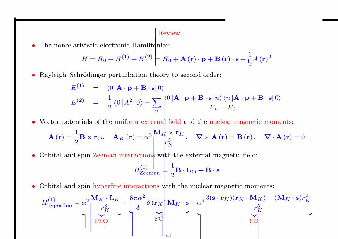
Review
• The nonrelativistic electronic Hamiltonian:
H = H0 + H(1) + H(2) = H0 + A (r) · p + B (r) · s +1
2A (r)2
• Rayleigh–Schrodinger perturbation theory to second order:
E(1) = 〈0 |A · p + B · s| 0〉
E(2) =1
2
˙0
˛˛A2
˛˛ 0
¸−
X
n
〈0 |A · p + B · s|n〉 〈n |A · p + B · s| 0〉
En − E0
• Vector potentials of the uniform external field and the nuclear magnetic moments:
A (r) =1
2B× rO, AK (r) = α2 MK × rK
r3K
, ∇×A (r) = B (r) , ∇ ·A (r) = 0
• Orbital and spin Zeeman interactions with the external magnetic field:
H(1)Zeeman =
1
2B · LO + B · s
• Orbital and spin hyperfine interactions with the nuclear magnetic moments:
H(1)hyperfine = α2 MK · LK
r3K
| z
PSO
+8πα2
3δ (rK)MK · s
| z
FC
+ α2 3(s · rK)(rK ·MK)− (MK · s)r2K
r5K
| z
SD
36

Gauge transformation of the Schrodinger equation
• Consider a general gauge transformation:
A′ = A + ∇f, φ′ = φ−∂f
∂t
• It can be shown that the Hamiltonian then transforms in the following manner
H′ = H +∂f
∂t,
which constitutes a unitary transformation:„
H′ − i∂
∂t
«
= exp (−if)
„
H − i∂
∂t
«
exp (if)
• In order that the Schrodinger equation is still satisfied„
H′ − i∂
∂t
«
Ψ′ ⇔
„
H − i∂
∂t
«
Ψ,
the new wave function must be related to the old one by a compensating unitary
transformation:
Ψ′ = exp (−if) Ψ
• No observable properties such as the electron density are then affected:
ρ′ = (Ψ′)∗Ψ′ = [Ψ exp(−if)]∗[exp(−if)Ψ] = Ψ∗Ψ = ρ
37
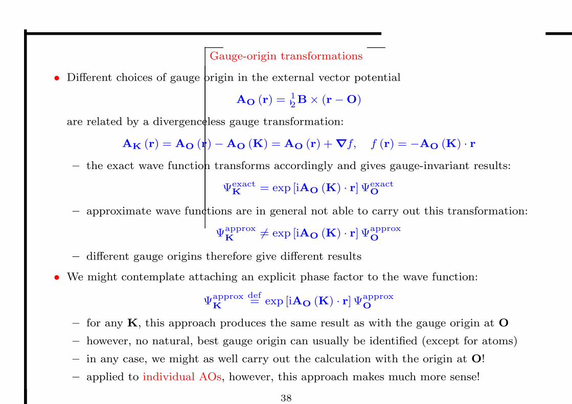
Gauge-origin transformations
• Different choices of gauge origin in the external vector potential
AO (r) = 12B× (r−O)
are related by a divergenceless gauge transformation:
AK (r) = AO (r)−AO (K) = AO (r) + ∇f, f (r) = −AO (K) · r
– the exact wave function transforms accordingly and gives gauge-invariant results:
ΨexactK
= exp [iAO (K) · r] ΨexactO
– approximate wave functions are in general not able to carry out this transformation:
ΨapproxK
6= exp [iAO (K) · r] ΨapproxO
– different gauge origins therefore give different results
• We might contemplate attaching an explicit phase factor to the wave function:
ΨapproxK
def= exp [iAO (K) · r] Ψapprox
O
– for any K, this approach produces the same result as with the gauge origin at O
– however, no natural, best gauge origin can usually be identified (except for atoms)
– in any case, we might as well carry out the calculation with the origin at O!
– applied to individual AOs, however, this approach makes much more sense!
38

Natural gauge origin for AOs
• Assume AOs positioned at K with the following properties:
H0χlm = E0χlm, LKz χlm = mlχlm, LK = −i (r−K)×∇
• We first choose the gauge origin to be at K:
AK (r) =1
2B× (r−K)
– The AOs χlm are then correct to first order in B:
HK (B) χlm =
»
H0 +1
2BLK
z +O`B2
´–
χlm =
»
E0 +1
2mlB +O
`B2
´–
χlm
• Next, we put the gauge origin at O 6= K:
AO (r) =1
2B× (r−O)
– The AOs χlm are now correct only to zero order in B:
HO (B) χlm =
»
H0 +1
2BLO
z +O`B2
´–
χlm 6=
»
E0 +1
2mlB +O
`B2
´–
χlm
• Standard AOs are biased towards K!
39

London orbitals
• A traditional AO gives best description with the gauge origin at its position K.
• Attach to each AO a phase factor that represents the gauge-origin transformation to its
position K from the global origin O:
ωlm = exp [iAK (O) · r] χlm = expˆi 12B× (O−K) · r
˜χlm
• Each AO now behaves as if the global gauge origin were at its position!
• In particular, all AOs are now correct to first order in B, for any global origin O.
• The calculations become gauge-origin independent and uniform (good) quality is
guaranteed.
• These are the London orbitals (1937), also known as GIAOs (gauge-origin independent
AOs).
40
Review
• The nonrelativistic electronic Hamiltonian:
H = H0 + H(1) + H(2) = H0 + A (r) · p + B (r) · s +1
2A (r)2
• Rayleigh–Schrodinger perturbation theory to second order:
E(1) = 〈0 |A · p + B · s| 0〉
E(2) =1
2
˙0
˛˛A2
˛˛ 0
¸−
X
n
〈0 |A · p + B · s|n〉 〈n |A · p + B · s| 0〉
En − E0
• Vector potentials of the uniform external field and the nuclear magnetic moments:
A (r) =1
2B× rO, AK (r) = α2 MK × rK
r3K
, ∇×A (r) = B (r) , ∇ ·A (r) = 0
• Orbital and spin Zeeman interactions with the external magnetic field:
H(1)Zeeman =
1
2B · LO + B · s
• Orbital and spin hyperfine interactions with the nuclear magnetic moments:
H(1)hyperfine = α2 MK · LK
r3K
| z
PSO
+8πα2
3δ (rK)MK · s
| z
FC
+ α2 3(s · rK)(rK ·MK)− (MK · s)r2K
r5K
| z
SD
41

Taylor expansion of the energy
• Expand the energy in the presence of an external magnetic field B and nuclear magnetic
moments MK around zero field and zero moments:
E (B,M) = E0 +
perm. magnetic momentsz |
BTE(10) +
hyperfine couplingz | X
K
MTKE
(01)K
+1
2BTE(20)B
| z
− magnetizability
+1
2
X
K
BTE(11)K MK
| z
shieldings + 1
+1
2
X
KL
MTKE
(02)KL ML
| z
spin–spin couplings
+ · · ·
• The first-order terms vanish for closed-shell systems because of symmetry:D
c.c.˛˛˛ Ωimaginary
˛˛˛ c.c.
E
≡D
c.c.˛˛˛ Ωtriplet
˛˛˛ c.c.
E
≡ 0
• Higher-order terms are negligible since the perturbations are tiny:
1) the magnetic induction B is weak (≈ 10−5 a.u.)
2) the nuclear magnetic moments MK are small (µ0µN ≈ 10−8 a.u.)
• We shall therefore consider only the second-order terms:
the magnetizability, the shieldings, and the spin–spin couplings
42
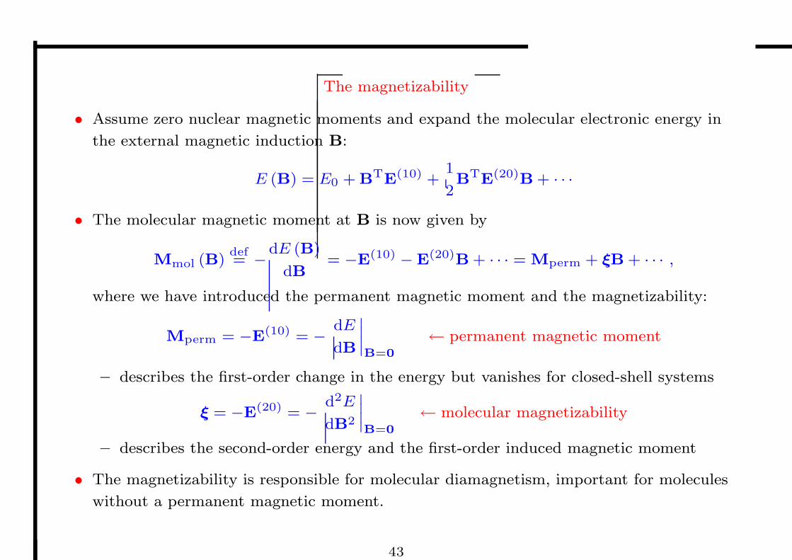
The magnetizability
• Assume zero nuclear magnetic moments and expand the molecular electronic energy in
the external magnetic induction B:
E (B) = E0 + BTE(10) +1
2BTE(20)B + · · ·
• The molecular magnetic moment at B is now given by
Mmol (B)def= −
dE (B)
dB= −E(10) −E(20)B + · · · = Mperm + ξB + · · · ,
where we have introduced the permanent magnetic moment and the magnetizability:
Mperm = −E(10) = −dE
dB
˛˛˛˛B=0
← permanent magnetic moment
– describes the first-order change in the energy but vanishes for closed-shell systems
ξ = −E(20) = −d2E
dB2
˛˛˛˛B=0
← molecular magnetizability
– describes the second-order energy and the first-order induced magnetic moment
• The magnetizability is responsible for molecular diamagnetism, important for molecules
without a permanent magnetic moment.
43

The calculation of magnetizabilities
• The molecular magnetizability of a closed-shell system:
ξ = −d2E
dB2= −
fi
0
˛˛˛˛
∂2H
∂B2
˛˛˛˛ 0
fl
+ 2X
n
D
0˛˛˛
∂H∂B
˛˛˛ n
E D
n˛˛˛
∂H∂B
˛˛˛ 0
E
En − E0
=1
4
D
0˛˛˛rOrT
O−
“
rTO
rO
”
I3
˛˛˛ 0
E
| z
diamagnetic term
+1
2
X
n
〈0 |LO|n〉˙n
˛˛LT
O
˛˛ 0
¸
En − E0| z
paramagnetic term
• The (often) dominant diamagnetic term arises from differentiation of the operator:
1
2A2 (B) =
1
8(B× rO) · (B× rO) =
1
8
ˆB2r2
O− (B · rO)(B · rO)
˜
– the isotropic part of the diamagnetic contribution is given by:
ξdia =1
3Trξdia = −
1
6
˙0
˛˛x2
O+ y2
O+ z2
O
˛˛ 0
¸= −
1
6
˙0
˛˛r2
O
˛˛ 0
¸← system surface
• Only the orbital Zeeman interaction contributions to the paramagnetic term:
S |0〉 ≡ 0 ← singlet state
– for 1S systems (closed-shell atoms), the paramagnetic term vanishes altogether:
12LO
˛˛1S
¸≡ 0 ← gauge origin at nucleus
44

Hartree–Fock magnetizabilities
• Basis-set requirements for magnetizatibilities are modest if London orbitals are used:
basis cc-pVDZ cc-pVTZ cc-pVQZ
HF basis-set error 2.8% 1.0% 0.4%
• The HF model overestimates the magnitude of magnetizabilities by 5%–10%:
10−30 JT−2 HF exp. diff.
H2O −232 −218 −6.4%
NH3 −289 −271 −6.6%
CH4 −315 −289 −9.0%
CO2 −374 −349 −7.2%
PH3 −441 −435 −1.4%
H2S −446 −423 −5.4%
C3H4 −482 −420 −14.8%
CSO −595 −538 −10.6%
CS2 −752 −701 −7.3%
– compare with polarizabilities, which require large basis sets and are underestimated
45

High-resolution NMR spin Hamiltonian
• Consider a molecule in the presence of an external field B along the z axis and with
nuclear spins IK related to the nuclear magnetic moments MK as:
MK = γK hIK ≈ 10−4 a.u.
where γK is the magnetogyric ratio of the nucleus.
• Assuming free molecular rotation, the nuclear magnetic energy levels can be reproduced
by the following high-resolution NMR spin Hamiltonian:
HNMR = −X
K
γK h(1− σK)BIKz
| z
nuclear Zeeman interaction
+X
K>L
γKγLh2KKLIK · IL
| z
nuclear spin–spin interaction
where we have introduced
– the nuclear shielding constants σK
– the (reduced) indirect nuclear spin–spin coupling constants KKL
• This is an effective nuclear spin Hamiltonian:
– it reproduces NMR spectra without considering the electrons explicitly
– the spin parameters σK and KKL are adjusted to fit the observed spectra
– we shall consider their evaluation from molecular electronic-structure theory
46

Simulated 200 MHz NMR spectra of vinyllithium
0 100 200
MCSCF
0 100 200 0 100 200
B3LYP
0 100 200
0 100 200
experiment
0 100 200 0 100 200
RHF
0 100 200
47

Nuclear shielding constants
• Recall the energy expansion for a closed-shell molecule in the presence of an external
field B and nuclear magnetic moments MK :
E (B,M) = E0 +1
2BTE(20)B +
1
2
X
K
BTE(11)K MK +
1
2
X
KL
MTKE
(02)KL ML + · · ·
• In this expansion, E(11)K describes the coupling between the applied field and the nuclear
magnetic moments:
– in the absence of electrons (i.e., in vacuum), this coupling is identical to −I3:
HnucZeeman = −B ·
X
K
MK ← the purely nuclear Zeeman interaction
– in the presence of electrons (i.e., in a molecule), the coupling is modified slightly:
E(11)K = −I3 + σK ← the nuclear shielding tensor
• Since the nuclear shielding constants arise from a hyperfine interaction between the
electrons and the nuclei, it is proportional to α2 ≈ 5 · 10−5 and is measured in ppm.
• The nuclear Zeeman interaction, which does not enter the electronic problem, has here
been introduced in a purely ad hoc fashion. Its status is otherwise similar to that of the
Coulomb nuclear–nuclear repulsion operator.
48

The calculation of nuclear shielding tensors
• Nuclear shielding tensors of a closed-shell system:
σK =d2Eel
dBdMK
=
fi
0
˛˛˛˛
∂2H
∂B∂MK
˛˛˛˛ 0
fl
− 2X
n
D
0˛˛˛
∂H∂B
˛˛˛ n
E D
n˛˛˛
∂H∂MK
˛˛˛ 0
E
En − E0
=α2
2
*
0
˛˛˛˛˛
rTO
rKI3 − rOrTK
r3K
˛˛˛˛˛0
+
| z
diamagnetic term
−α2X
n
˙0
˛˛L
O
˛˛ n
¸ D
n˛˛˛r−3
K LTK
˛˛˛ 0
E
En − E0| z
paramagnetic term
• The (usually) dominant diamagnetic term arises from differentiation of the operator:
A (B) ·A (MK) =1
2α2r−3
K (B× rO) · (MK × rK)
• As for the magnetizability, there is no spin contribution for singlet states:
S |0〉 ≡ 0 ← singlet state
• For 1S systems (closed-shell atoms), the paramagnetic term vanishes completely and the
the shielding is given by (assuming gauge origin at the nucleus):
σLamb =1
3α2
D1S
˛˛˛r
−1K
˛˛˛1S
E
← Lamb formula
49

Benchmark calculations of BH shieldings
HF MP2 CCSD CCSD(T) FCI
σ(11B) −261.3 −220.7 −166.6 −170.5 −170.1
σ(1H) 24.21 24.12 24.74 24.62 24.60
∆σ(11B) 690.1 629.9 549.4 555.2 554.7
∆σ(1H) 14.15 14.24 13.52 13.69 13.70
• TZP+ basis, RBH = 123.24 pm
• J. Gauss and K. Ruud, Int. J. Quantum Chem. S29 (1995) 437
• J. Gauss and J. F. Stanton, J. Chem. Phys. 104 (1996) 2574
50

Calculated and experimental equilibrium shielding constants
HF CAS MP2 CCSD CCSD(T) exp.
HF F 413.6 419.6 424.2 418.1 418.6 410± 6
H 28.4 28.5 28.9 29.1 29.2 28.5± 0.2
H2O O 328.1 335.3 346.1 336.9 337.9 344± 17
H 30.7 30.2 30.7 30.9 30.9 30.05± 0.02
NH3 N 262.3 269.6 276.5 269.7 270.7 264.5
H 31.7 31.0 31.4 31.6 31.6 31.2± 1.0
CH4 C 194.8 200.4 201.0 198.7 198.9 198.7
H 31.7 31.2 31.4 31.5 31.6 30.61
F2 F −167.9 −136.6 −170.0 −171.1 −186.5 −192.8
N2 N −112.4 −53.0 −41.6 −63.9 −58.1 −61.6± 0.2
CO C −25.5 8.2 10.6 0.8 5.6 3.0± 0.9
O −87.7 −38.9 −46.5 −56.0 −52.9 −42.3± 17
• For references and details, see Helgaker, Jaszunski, and Ruud, Chem. Rev. 99 (1999)
293.
51

DFT shielding constants
HF LDA BLYP B3LYP KT2 CCSD(T) exp.
HF F 413.6 416.2 401.0 408.1 411.4 418.6 410± 6
H2O O 328.1 334.8 318.2 325.0 329.5 337.9 344± 17
NH3 N 262.3 266.3 254.6 259.2 264.6 270.7 264.5
CH4 C 194.8 193.1 184.2 188.1 195.1 198.9 198.7
F2 F −167.9 −284.2 −336.7 −208.3 −211.0 −186.5 −192.8
N2 N −112.4 −91.4 −89.8 −86.4 −59.7 −58.1 −61.6± 0.2
CO C −25.5 −20.3 −19.3 −17.5 7.4 5.6 3.0± 0.9
O −87.7 −87.5 −85.4 −78.1 −57.1 −52.9 −42.3± 17
52
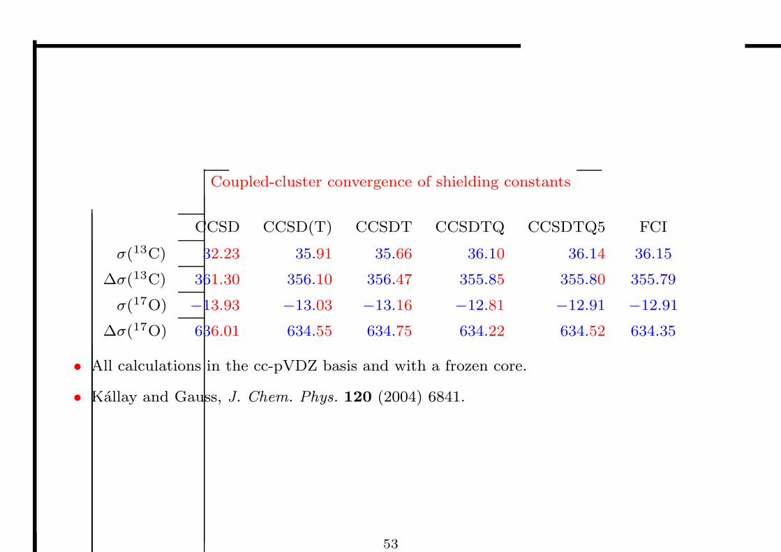
Coupled-cluster convergence of shielding constants
CCSD CCSD(T) CCSDT CCSDTQ CCSDTQ5 FCI
σ(13C) 32.23 35.91 35.66 36.10 36.14 36.15
∆σ(13C) 361.30 356.10 356.47 355.85 355.80 355.79
σ(17O) −13.93 −13.03 −13.16 −12.81 −12.91 −12.91
∆σ(17O) 636.01 634.55 634.75 634.22 634.52 634.35
• All calculations in the cc-pVDZ basis and with a frozen core.
• Kallay and Gauss, J. Chem. Phys. 120 (2004) 6841.
53

Nuclear spin–spin couplings
• The last term in the expansion of the molecular electronic energy in B and MK
E (B,M) = E0 + 12BTE(20)B + 1
2
P
K BTE(11)K MK + 1
2
P
KL MTKE
(02)KL ML + · · ·
describes the coupling of the nuclear magnetic moments in the presence of electrons.
• There are two distinct contributions to the coupling:
the direct and indirect contributions
E(02)KL = DKL + KKL
• The direct coupling occurs by a classical dipole mechanism:
DKL = α2R−5KL
`R2
KLI3 − 3RKLRTKL
´≈ 10−12 a.u.
– it is anisotropic and vanishes in isotropic media such as gases and liquids
• The indirect coupling arises from hyperfine interactions with the surrounding electrons:
– it is exceedingly small: KKL ≈ 10−16 a.u. ≈ 1 Hz
– it does not vanish in isotropic media
– it gives the fine structure of high-resolution NMR spectra
• Experimentalists usually work in terms of the (nonreduced) spin–spin couplings
JKL = h γK
2π
γL
2πKKL ← isotope dependent
54

The calculation of indirect nuclear spin–spin coupling tensors
• The indirect nuclear spin–spin coupling tensor of a closed-shell system is given by:
KKL =d2Eel
dMKdML
=
fi
0
˛˛˛˛
∂2H
∂MK∂ML
˛˛˛˛ 0
fl
− 2X
n
D
0˛˛˛
∂H∂MK
˛˛˛ n
E D
n˛˛˛
∂H∂ML
˛˛˛ 0
E
En − E0
• Carrying out the differentiation, we obtain:
KKL = α4
*
0
˛˛˛˛˛
rTKrLI3 − rKrT
L
r3Kr3
L
˛˛˛˛˛0
+
| z
diamagnetic spin–orbit (DSO)
− 2α4X
n
D
0˛˛˛r
−3K LK
˛˛˛ n
E D
n˛˛˛r
−3L LT
L
˛˛˛ 0
E
En − E0| z
paramagnetic spin–orbit (PSO)
− 2α4X
n
fi
0
˛˛˛˛8π3
δ(rK)s +3rKr
TK
−r2K
I3
r5K
s
˛˛˛˛ n
fl fi
n
˛˛˛˛8π3
δ(rL)sT+3rLr
TL−r2
LI3
r5L
sT˛˛˛˛ 0
fl
En − E0| z
Fermi contact (FC) and spin–dipole (SD)
– the isotropic FC/FC term often dominates short-range coupling constants
– the FC/SD and SD/FC terms often dominate the anisotropic part of KKL
– the orbital contributions (especially DSO) are usually but not invariably small
– for large internuclear separations, the DSO and PSO contributions cancel
55

Calculations of indirect nuclear spin–spin coupling constants
• The calculation of spin–spin coupling constants is a challenging task:
– triplet as well as singlet perturbations are involved
– electron correlation important—the Hartree–Fock model fails abysmally
– the dominant FC contribution requires an accurate description of the electron
density at the nuclei (large decontracted s sets)
• We must solve a large number of response equations:
– 3 singlet equations and 7 triplet equations for each nucleus
– for shieldings, only 3 equations are required, for molecules of all sizes
• Spin–spin couplings are very sensitive to the molecular geometry:
– equilibrium structures must be chosen carefully
– large vibrational corrections (often 5%–10%)
• However, unlike in shielding calculations, there is no need for London orbitals since no
external magnetic field is involved.
• For heavy elements, a relativistic treatment may be necessary.
56

Relative importance of the contributions to spin–spin coupling constants
• The isotropic indirect spin–spin coupling constants can be uniquely decomposed as:
JKL = JDSOKL + JPSO
KL + JFCKL + JSD
KL
• The spin–spin coupling constants are often dominated by the FC term.
• Since the FC term is relatively easy to calculate, it is tempting to ignore the other terms.
• However, none of the contributions can be a priori neglected (N2 and CO)!
H2 HF H2OO-H
NH3N-H
CH4C-H
C2H4C-C
HCNN-C
N2 CO C2H2C-C
-100
0
100
200
FCFC
FC FC FC FCFC FC FC
FCPSO
PSO
PSOSD
SD
SD
57

RHF and the triplet instability problem
• RHF does not in general work for spin–spin calculations:
– the RHF wave function often becomes triplet unstable
– at or close to such instabilities, the RHF description of
spin interactions becomes unphysical
– the spin–spin coupling constants of C2H4:
Hz 1JCC1JCH
2JCH2JHH
3Jcis3Jtrans
exp. 68 156 −2 2 12 19
RHF 1270 755 −572 −344 360 400
CAS 76 156 −1 3 14 211 2 3 4 5 6 7
-1
1
2
1 2 3 4 5 6 7
-1.0
-0.8
-0.6
• Indeed, any method based on the RHF reference state may have problems:
– 1JCN in HCN [Auer and Gauss, JCP 115 (2001) 1619]
Hz RHF CCSD CCSD(T) CC3 CCSDT
relaxed −92.0 −8.1 7.4 −2.6 −14.5
unrelaxed −15.0 −14.7 −14.6
– in CC theory, orbital relaxation should be treated through singles amplitudes
– noniterative CCSD(T) should not be used; use iterative CC3 instead
– all electrons should be correlated in unrelaxed CC calculations
58

Reduced spin–spin coupling constants (1019kg m−2 s−2A−2)
RHF CAS RAS SOPPA CCSD CC3 exp∗ vib
HF 1JHF 59.2 48.0 48.1 46.8 46.1 46.1 47.6 −3.4
CO 1JCO 13.4 −28.1 −39.3 −45.4 −38.3 −37.3 −38.3 −1.7
N21JNN 175.0 −5.7 −9.1 −23.9 −20.4 −20.4 −19.3 −1.1
H2O 1JOH 63.7 51.5 47.1 49.5 48.4 48.2 52.8 −3.3
2JHH −1.9 −0.8 −0.6 −0.7 −0.6 −0.6 −0.7 0.1
NH31JNH 61.4 48.7 50.2 51.0 48.1 50.8 −0.3
2JHH −1.9 −0.8 −0.9 −0.9 −1.0 −0.9 0.1
C2H41JCC 1672.0 99.6 90.5 92.5 92.3 87.8 1.2
1JCH 249.7 51.5 50.2 52.0 50.7 50.0 1.7
2JCH −189.3 −1.9 −0.5 −1.0 −1.0 −0.4 −0.4
2JHH −28.7 −0.2 0.1 0.1 0.0 0.2 0.0
3Jcis 30.0 1.0 1.0 1.0 1.0 0.9 0.1
3Jtns 33.3 1.5 1.5 1.5 1.5 1.4 0.2˛˛∆
˛˛ abs. 180.3 3.3 1.6 1.8 1.2 1.6 ∗at Re
% 5709 60 14 24 23 6
59
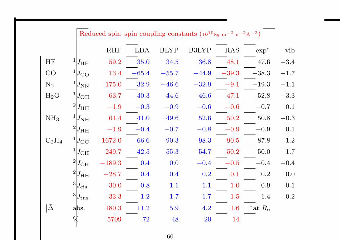
Reduced spin–spin coupling constants (1019kg m−2 s−2A−2)
RHF LDA BLYP B3LYP RAS exp∗ vib
HF 1JHF 59.2 35.0 34.5 36.8 48.1 47.6 −3.4
CO 1JCO 13.4 −65.4 −55.7 −44.9 −39.3 −38.3 −1.7
N21JNN 175.0 32.9 −46.6 −32.9 −9.1 −19.3 −1.1
H2O 1JOH 63.7 40.3 44.6 46.6 47.1 52.8 −3.3
2JHH −1.9 −0.3 −0.9 −0.6 −0.6 −0.7 0.1
NH31JNH 61.4 41.0 49.6 52.6 50.2 50.8 −0.3
2JHH −1.9 −0.4 −0.7 −0.8 −0.9 −0.9 0.1
C2H41JCC 1672.0 66.6 90.3 98.3 90.5 87.8 1.2
1JCH 249.7 42.5 55.3 54.7 50.2 50.0 1.7
2JCH −189.3 0.4 0.0 −0.4 −0.5 −0.4 −0.4
2JHH −28.7 0.4 0.4 0.2 0.1 0.2 0.0
3Jcis 30.0 0.8 1.1 1.1 1.0 0.9 0.1
3Jtns 33.3 1.2 1.7 1.7 1.5 1.4 0.2˛˛∆
˛˛ abs. 180.3 11.2 5.9 4.2 1.6 ∗at Re
% 5709 72 48 20 14
60
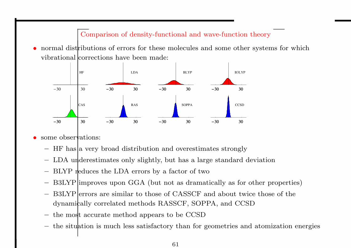
Comparison of density-functional and wave-function theory
• normal distributions of errors for these molecules and some other systems for which
vibrational corrections have been made:
-30 30
CAS
-30 30 -30 30
RAS
-30 30 -30 30
SOPPA
-30 30 -30 30
CCSD
-30 30
-30 30
HF
-30 30
LDA
-30 30 -30 30
BLYP
-30 30 -30 30
B3LYP
-30 30
• some observations:
– HF has a very broad distribution and overestimates strongly
– LDA underestimates only slightly, but has a large standard deviation
– BLYP reduces the LDA errors by a factor of two
– B3LYP improves upon GGA (but not as dramatically as for other properties)
– B3LYP errors are similar to those of CASSCF and about twice those of the
dynamically correlated methods RASSCF, SOPPA, and CCSD
– the most accurate method appears to be CCSD
– the situation is much less satisfactory than for geometries and atomization energies
61

Trends in spin–spin coupling constants
• comparison of calculated (red) and B3LYP (blue) spin–spin coupling
constants
– plotted in order of decreasing experimental value
-100
100
200
300
400
500
-20
-10
10
20
• trends are quite well reproduced by B3LYP, in particular for large couplings
62

Basis-set requirements
• Accurate spin–spin calculations require large basis sets, augmented with steep s functions
– Huz-III-su0: [11s6p2d/6s2p]
– Huz-III-su3: [14s6p2d/9s2p]
• B3LYP calculations on benzene with and without added s functions:
Hz MCSCF B3LYP-su3 B3LYP-su0 emp
1JCC 70.9 60.0 56.7 56.1
2JCC −5.0 −1.8 −1.7 −1.7
3JCC 19.1 11.2 10.7 9.4
1JCH 176.7 166.3 151.7 152.7
2JCH −7.4 2.0 1.7 1.4
3JCH 11.7 8.0 7.3 7.0
4JCH −1.3 −1.2 −1.3 −1.0
3JHH 8.7 7.6 7.0
4JHH 1.3 1.1 1.2
5JHH 0.8 0.7 0.6
• Cancellation of errors gives excellent agreement without added steep functions :)
63

The Karplus curve
• Vicinal couplings depend critically on the dihedral angle:
•3JHH in ethane as a function of the dihedral angle:
25 50 75 100 125 150 175
2
4
6
8
10
12
14
DFT
empirical
• The agreement with the empirical Karplus curve is good.
64
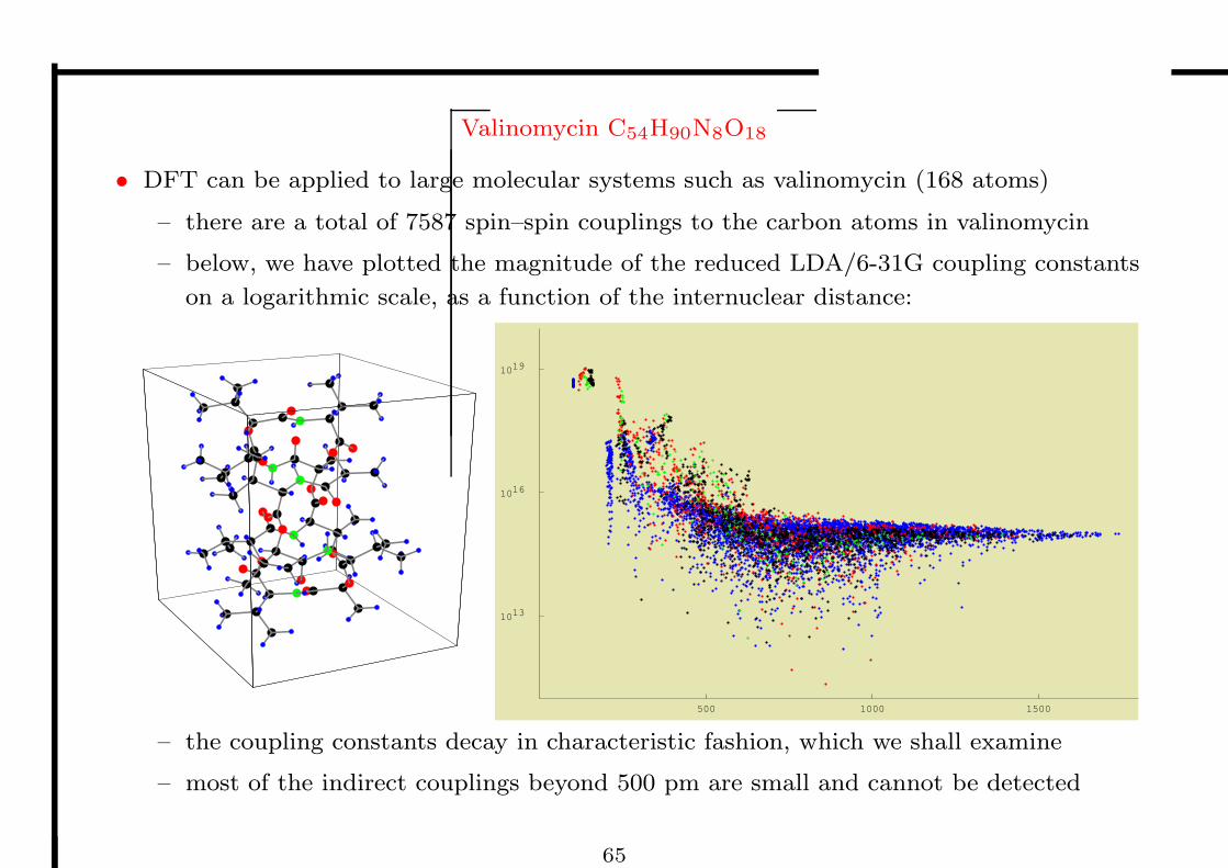
Valinomycin C54H90N8O18
• DFT can be applied to large molecular systems such as valinomycin (168 atoms)
– there are a total of 7587 spin–spin couplings to the carbon atoms in valinomycin
– below, we have plotted the magnitude of the reduced LDA/6-31G coupling constants
on a logarithmic scale, as a function of the internuclear distance:
500 1000 1500
1019
1016
1013
– the coupling constants decay in characteristic fashion, which we shall examine
– most of the indirect couplings beyond 500 pm are small and cannot be detected
65

Valinomycin LDA/6-31G spin–spin couplings to CH, CO, CN, CC greater than 0.01 Hz
100 200 300 400 500 600
100
30
10
3
1
0.3
0.1
0.03
66

Valinomycin LDA/6-31G spin–spin couplings to CH, CO, CN, CC greater than 0.01 Hz
100 200 300 400 500 600
100
30
10
3
1
0.3
0.1
0.03
67

Valinomycin LDA/6-31G spin–spin couplings to CH, CO, CN, CC greater than 0.01 Hz
100 200 300 400 500 600
100
30
10
3
1
0.3
0.1
0.03
68

Valinomycin LDA/6-31G spin–spin couplings to CH, CO, CN, CC greater than 0.01 Hz
100 200 300 400 500 600
100
30
10
3
1
0.3
0.1
0.03
69

Valinomycin LDA/6-31G spin–spin couplings to CH, CO, CN, CC greater than 0.01 Hz
100 200 300 400 500 600
100
30
10
3
1
0.3
0.1
0.03
70

The different long-range decays of the Ramsey terms
• Letting M be the center of the product Gaussian GaGb, we obtainD
Ga
˛
˛
˛hFCK
˛
˛
˛ Gb
E
∝ exp“
−µR2KM
”
,D
Ga
˛
˛
˛hSDK
˛
˛
˛ Gb
E
∝ R−3KM
,
D
Ga
˛
˛
˛hDSOKL
˛
˛
˛ Gb
E
∝ R−2KM
R−2LM
,D
Ga
˛
˛
˛hPSOK
˛
˛
˛ Gb
E
∝ R−2KM
• Insertion in Ramsey’s expression gives (red positive, blue negative)
500 1000 1500
1019
1016
1013
DSO decays as R-2
negative
500 1000 1500
1019
1016
1013
PSO decays as R-2
positive
500 1000 1500
1019
1016
1013
FC decays exponentially
mixed signs
500 1000 1500
1019
1016
1013
SD decays as R-3
mixed signs
71

The long-range orbital contributions
• At large separations, the couplings are dominated by the orbital contributions:
JDSOKL ∝ R−2
KL, JPSOKL ∝ R−2
KL ← large separations
• Moreover, in this limit, the DSO contributions all become negative:
KDSOKL = 2α4
3
D
0˛˛˛r
−3K r−3
L rK · rL
˛˛˛ 0
E
< 0 ← large separations
• Also, the PSO contributions become positive, nearly cancelling the DSO contributions.
– use of Taylor expansion, the virial theorem, and the resolution of identity give:
JDSOKL + JPSO
KL ∝ R−3KL ← large separations, large basis
• However, the PSO contributions converge very slowly to the basis-set limit:
500 1000 1500103
1
10-3
10-7LDA6-31G
500 1000 1500103
1
10-3
10-7LDAHII
72


