
Modelling stellar atmosphereswith full Zeeman treatment
Katharina M. Bischof, Martin J. Stift
M. J. Stift’s Supercomputing GroupFWF project P16003
Institute f. AstronomyVienna, Austria
CP#AP workshop 12th of September 2007
1 / 16

MotivationThe CAMAS Code
Findings
Contents
1 Motivation
2 The CAMAS Code
3 Findings
2 / 16

MotivationThe CAMAS Code
Findings
Contents
1 Motivation
2 The CAMAS Code
3 Findings
2 / 16

MotivationThe CAMAS Code
Findings
Contents
1 Motivation
2 The CAMAS Code
3 Findings
2 / 16

MotivationThe CAMAS Code
FindingsOutline of the problem
Outline of the problem
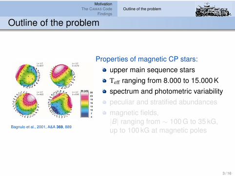
Bagnulo et al., 2001, A&A 369, 889
Properties of magnetic CP stars:upper main sequence starsTeff ranging from 8.000 to 15.000 Kspectrum and photometric variabilitypeculiar and stratified abundancesmagnetic fields,|B| ranging from ∼ 100 G to 35 kG,up to 100 kG at magnetic poles
3 / 16
MotivationThe CAMAS Code
FindingsOutline of the problem
Outline of the problem
Bagnulo et al., 2001, A&A 369, 889
Properties of magnetic CP stars:upper main sequence starsTeff ranging from 8.000 to 15.000 Kspectrum and photometric variabilitypeculiar and stratified abundancesmagnetic fields,|B| ranging from ∼ 100 G to 35 kG,up to 100 kG at magnetic poles
3 / 16

MotivationThe CAMAS Code
FindingsOutline of the problem
Outline of the problem
requirements specification for the atmospheric model codetemperature range (of interest): 8.000 to 15.000 Kpeculiar and stratified abundancesarbitrary inclination of the field in plane parallel modelsfull Zeeman treatment, polarised Feautrier solverhydrostatic equilibrium with magnetic pressureVALD line data, CoCoSsimplifications: plane parallel, Kurucz continuum routines,no dynamic phenomena considered, no microturbulence.
4 / 16

MotivationThe CAMAS Code
Findings
Software engineeringPolarised radiation transferTemperature correction
The CAMAS Code
Program features:ATLAS12 continua for comparabilitywith standard modelsconsistent with spectral synthesis(COSSAM) and radiative diffusion(CARAT) codewritten in Ada95thread parallelmodularised, object oriented
5 / 16

MotivationThe CAMAS Code
Findings
Software engineeringPolarised radiation transferTemperature correction
Polarised radiation transfer equation
ddz I = −K I + K (S,0,0,0)†
Stokes vectorI = (I,Q,U,V )†
absorption matrixK = κc 1 + κo Φ
line absorption matrix
Φ =
φI φQ φU φVφQ φI φ
′
V −φ′UφU −φ′V φI φ
′
QφV φ
′
U −φ′Q φI
γ
χ
~B
~x ′ ~y ′
~z ′,~I
Show details
6 / 16

MotivationThe CAMAS Code
Findings
Software engineeringPolarised radiation transferTemperature correction
Zeeman Feautrier solver
Feautrier equation can be generalised to the magneticcase in the presence of blends (see Alecian and Stift, 2004, A&A
416, 703)
d~Jdτ5000
= X~H and d~Hdτ5000
= X(~J − ~S) with X := Kκ5000µ
ddτ5000
(X−1 d~Jdτ5000
) = X(~J − ~S) (inner points)
dX−1
dτ5000
d~Jdτ5000
+ X−1 d2~Jdτ2
5000= X(~J − ~S) (boundary condition)
N equations, N unknowns
B1~J1 − C1
~J2 = ~L1
− An ~Jn−1 + Bn ~Jn − Cn ~Jn+1 = ~Ln
− AN~JN−1 + BN
~JN = ~LN
7 / 16

MotivationThe CAMAS Code
Findings
Software engineeringPolarised radiation transferTemperature correction
Temperature correction
Dreizler’s Lucy Unsold scheme adapted for polarised radiationtransport equations:(see Dreizler, 2003, ASPC 288, 69)
momenta of the polarised radiation transport equationdifferences (∆X = XEquilibrium − XModel) of flux, intensity andradiation pressuretwo flux criteria
local balance of emitted versus absorbed energyd(HI )zdτ5000
= 0 (constant flux)cannot be used in deep layers where the atmospherebecomes diffusive and S ∼ J ∼ local Planck function.nonlocal condition of constant flux:∞∫0
∮HIdΩdν − σ
4πT 4eff = 0 (desired value of the flux)
inefficient in regions with small opacitiesShow momenta
8 / 16

MotivationThe CAMAS Code
Findings
Software engineeringPolarised radiation transferTemperature correction
Combining the flux criteria
∆T =π
4σT 3„d1
„SR∞
0 [Kν~Jν ]IdνR∞0 [Kν ]I,ISνdν
− S«
| z local energy conservation
+ d2SR∞
0 [Kν~Jν ]IdνJIR∞
0 [Kν ]I,ISνdνf0∆HI(0)
fg| z surface flux
+ d3SR∞
0 [Kν~Jν ]IdνJIR∞
0 [Kν ]I,ISνdν1fZ τ
0
R∞0 [Kν ~Hν ]Idν
HIκ5000∆HIdτ5000| z
global energy conservation
«
9 / 16

MotivationThe CAMAS Code
Findings
Comparison with Carpenter’s resultsComparisons with LLMODELS
Summary
Results and comparisons
Two effectsenhanced line blanketingmagnetic pressure
Comparison with the results ofCarpenter (enhanced line blanketing and magneticpressure see Carpenter, 1985, ApJ 289, 660, Carpenter, 1983, PhD Thesis )LLMODELS (enhanced line blanketing, see Kochukhov et al., 2005,
A&A 433, 671, Khan and Shulyak, 2006a, A&A 448, 1153, Khan and Shulyak,
2006b, A&A 454, 933)
10 / 16

MotivationThe CAMAS Code
Findings
Comparison with Carpenter’s resultsComparisons with LLMODELS
Summary
Comparison with Carpenter’s results
CAMAS results Carpenter, 1985, ApJ 289, 660
11 / 16

MotivationThe CAMAS Code
Findings
Comparison with Carpenter’s resultsComparisons with LLMODELS
Summary
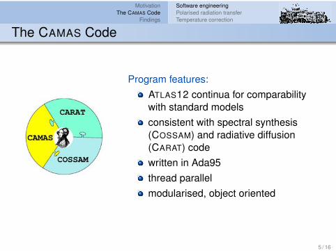
Comparisons with LLMODELS
differences between the field less and the “isotropic” model
CAMAS results Kochukhov et al., 2005, A&A 433, 671
12 / 16
MotivationThe CAMAS Code
Findings
Comparison with Carpenter’s resultsComparisons with LLMODELS
Summary
Comparisons with LLMODELS
differences between the field less and the “isotropic” model
CAMAS results Kochukhov et al., 2005, A&A 433, 671
12 / 16

MotivationThe CAMAS Code
Findings
Comparison with Carpenter’s resultsComparisons with LLMODELS
Summary
Depth scales
τross is affected by
(magnetic) line
blanketing, τ5000 is
not directly affected
13 / 16
MotivationThe CAMAS Code
Findings
Comparison with Carpenter’s resultsComparisons with LLMODELS
Summary
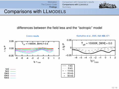
Depth scales
τross is affected by (magnetic) line blanketing, τ5000 is not directly affected
14 / 16
MotivationThe CAMAS Code
Findings
Comparison with Carpenter’s resultsComparisons with LLMODELS
Summary
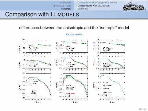
Comparison with LLMODELS
differences between the anisotropic and the “isotropic” modelCAMAS results
15 / 16
MotivationThe CAMAS Code
Findings
Comparison with Carpenter’s resultsComparisons with LLMODELS
Summary
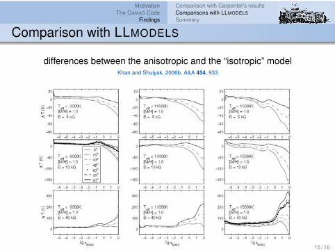
Comparison with LLMODELS
differences between the anisotropic and the “isotropic” modelKhan and Shulyak, 2006b, A&A 454, 933
15 / 16
MotivationThe CAMAS Code
Findings
Comparison with Carpenter’s resultsComparisons with LLMODELS
Summary
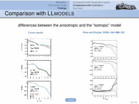
Comparison with LLMODELS
differences between the anisotropic and the “isotropic” model
CAMAS results Khan and Shulyak, 2006b, A&A 454, 933
Zoom15 / 16
MotivationThe CAMAS Code
Findings
Comparison with Carpenter’s resultsComparisons with LLMODELS
Summary
Summary
The Zeeman effect enhances the opacity. This affects theoptical depth and the temperature structure.CAMAS essentially confirms the results of LLMODELS. Theisotropic models are largely identical, however theanisotropic models with strong magnetic fields exhibitnotable differences that need to be clarified.The atmospheres computed with CAMAS will be used(among others) for the modelling of diffusion processes.
Acknowledgements: this work was supported by the Austrian Science Funds(FWF project P16003 of M.J.Stift). KMB wants to thank Bob Kurucz for theuseful discussions on the ATLAS code, Christian Stutz and the VALD team forthe line data and Holger Pikall for tree weeks of CPU-time.
16 / 16
AppendixReferences
Bibliography I
Alecian, G. and Stift, M. J.: 2004, A&A 416, 703Bagnulo, S., Wade, G. A., Donati, J.-F., Landstreet, J. D.,
Leone, F., Monin, D. N., and Stift, M. J.: 2001, A&A 369, 889Carpenter, K. G.: 1983, Ph.D. thesis, AA(Ohio State Univ.,
Columbus.)Carpenter, K. G.: 1985, ApJ 289, 660Dreizler, S.: 2003, in I. Hubeny, D. Mihalas, and K. Werner
(eds.), ASP Conf. Ser. 288: Stellar Atmosphere Modeling,Vol. 288 of ASP Conference Series, p. 69, Review oftemperature correction schemes, Damping
Khan, S. A. and Shulyak, D. V.: 2006a, A&A 448, 1153Khan, S. A. and Shulyak, D. V.: 2006b, A&A 454, 933Kochukhov, O., Khan, S., and Shulyak, D.: 2005, A&A 433, 671
17 / 16
AppendixReferences
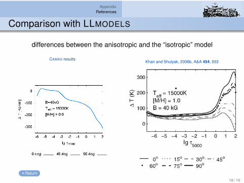
Comparison with LLMODELS
differences between the anisotropic and the “isotropic” model
CAMAS resultsKhan and Shulyak, 2006b, A&A 454, 933
Return
18 / 16

AppendixReferences
first depth point
d~Jdτ5000
|1 = X1(~J1 − (1− e−τ1X1)~S1)
~J1 = ~J2−∆τ(2,1)d~Jdτ |1−
(∆τ(2,1))2
2d2~Jdτ2 |1− . . . (“forward” Taylor series)
A1 = 0
B1 = 1 + ∆τ(2,1)X1 −(∆τ(2,1))2
2X1
dX−1
dτ5000|1X1 +
(∆τ(2,1))2
2X2
1
C1 = 1
~L1 = (∆τ(2,1) −(∆τ(2,1))2
2X1
dX−1
dτ5000|1)X1(1− e−τ1X1 )~S1 +
(∆τ(2,1))2
2X2
1~S1
19 / 16

AppendixReferences
inner depth points
ddτ
X−1 d~Jdτ
∣∣∣∣∣n
=X−1
n+ 12
~Jn+1−~Jn∆τ(n+1,n)
− X−1n− 1
2
~Jn−~Jn−1∆τ(n,n−1)
∆τ(n+1,n)+∆τ(n,n−1)
2
An =(Xn−1 + Xn)−1
∆τ(n,n−1)∆τ(n+1,n−1)
Bn =(Xn−1 − Xn)−1
∆τ(n,n−1)∆τ(n+1,n−1)+
(X−1n+1 + Xn)−1
∆τ(n+1,n)∆τ(n+1,n−1)+ Xn
Cn =(Xn+1 + Xn)−1
∆τ(n+1,n)∆τ(n+1,n−1)
~Ln = Xn~Sn
20 / 16

AppendixReferences
Flowchart of CAMAS
read input, initialiseenter radiative equilibrium loop
check convectionrecompute equidistant τ5000 and interpolate model data
← EXIT if convergence criteria are metpretabulate continua if necessaryreselect lines if necessaryenter integration loop (> 90% of computation time)
independent tasks use a magnetic Feautrier solver for allwavelength points and add the results
calculate temperature correctionscalculate and apply pressure correctionssearch for noise in the flux distribution and checkconvergenceapply temperature corrections if not converged yetapply Ng acceleration (optional)
21 / 16

AppendixReferences
Feautrier solver
solve radiation transport equation as boundary valueproblem
dI±
dτ5000= I± − S
define flux like and intensity like quantitiescombine equations for outward and inward raysdiscretize and add boundary conditions
22 / 16

AppendixReferences
Feautrier solver
solve radiation transport equation as boundary valueproblemdefine flux like and intensity like quantities
Hn =I+n − I−n
2, Jn =
I+n + I−n
2
combine equations for outward and inward raysdiscretize and add boundary conditions
22 / 16

AppendixReferences
Feautrier solver
solve radiation transport equation as boundary valueproblem
dI±
dτ5000= I± − S
define flux like and intensity like quantitiescombine equations for outward and inward rays
dJdτ5000
= H ,dH
dτ5000= J − S︸ ︷︷ ︸
d2Jdτ2
5000= J − S
discretize and add boundary conditions
22 / 16

AppendixReferences
Feautrier solver
solve radiation transport equation as boundary valueproblemdefine flux like and intensity like quantitiescombine equations for outward and inward raysdiscretize and add boundary conditions
I−(τ = 0) = 0, no incident radiation on the surface
dJdτ5000
|τ=0 = J(τ = 0)
HN = I+N − JN , diffusive at innermost depth-point
dJdτ5000
|N = I+N − JN with I+
N = SN +dS
dτ5000|N
22 / 16

AppendixReferences
Angle dependent opacity Return
line absorption terms
φI = 14 (2φp sin 2γ + (φr + φb)(1 + cos2 γ))
φQ = 14 (2φp − (φr + φb)) sin2 γ cos 2χ
φU = 14 (2φp − (φr + φb)) sin2 γ sin 2χ
φV = 12 (φr − φb) cos γ
φ p, b, r ... line absorption profiles
Faraday terms
φ′
Q = 14 (2φ
′p − (φ
′r + φ
′
b)) sin2 γ cos 2χ
φ′
U = 14 (2φ
′p − (φ
′r + φ
′
b)) sin2 γ sin 2χ
φ′
V = 12 (φ
′r − φ
′
b) cos γ
φ′
p, b, r ... anomalous dispersion profiles
θβ
ψ
~B~I
~x ~y
~z
γ
χ
~B
~x ′ ~y ′
~z ′,~I
23 / 16

AppendixReferences
Combining the flux criteria
0th moment: d∆HIdτ5000
=R∞
0 [Kν∆~Jν ]Idνκ5000
−R∞
0 [Kν ]I,I∆Sνdνκ5000
dHeq
dτ5000= 0, 0th moment for dHmod
dτ5000R∞0 [Kν~Xν,eq]I dν
Xeq∼
R∞0 [Kν~Xν,mod]I dν
Xmodel
∆S∆T = 4σT 3
π
4σT 3
π ∆T =S
R∞0 [Kν~Jν ]IdνR∞
0 [Kν ]I,ISνdν − S + SR∞0 [Kν ]I,ISνdν
R∞0 [Kν~Jν ]Idν
JI∆JI
1st moment: d∆KIdτ5000
=R∞
0 [Kν∆~Hν ]Idνκ5000
integrationvariable Eddington factors fτ = Kτ
Jτand g = H0
J0
f ∆JI︸︷︷︸∆KI
= f0g ∆HI(0) +
∫ τ0
R∞0 [Kν∆~Hν ]Idν
κ5000dτ5000
Return
24 / 16


![Theory of Stellar Atmospheres: An Introduction to ...assets.press.princeton.edu/releases/m10407.pdf · [72] L. Aller. Interpretation of normal stellar spectra. In Greenstein [1334],](https://cdn.vdocuments.mx/doc/165x107/5e0a49c4fdd6bd4d6062e3fe/theory-of-stellar-atmospheres-an-introduction-to-72-l-aller-interpretation.jpg)


