
1
MODELLING DAMAGE FOR ELASTOPLASTICITY
A THESIS SUBMITTED TOTHE GRADUATE SCHOOL OF NATURAL AND APPLIED SCIENCES
OFMIDDLE EAST TECHNICAL UNIVERSITY
BY
CELAL SOYARSLAN
IN PARTIAL FULFILLMENT OF THE REQUIREMENTSFOR
THE DEGREE OF DOCTOR OF PHILOSOPHYIN
CIVIL ENGINEERING
DECEMBER 2008

Approval of the thesis:
MODELLING DAMAGE FOR ELASTOPLASTICITY
submitted by CELAL SOYARSLAN in partial fulfillment of the requirements forthe degree ofDoctor of Philosophy in Civil Engineering Department, Middle East Tech-nical University by,
Prof. Dr. Canan OzgenDean, Graduate School of Natural and Applied Sciences
Prof. Dr. Guney OzcebeHead of Department, Civil Engineering
Assoc. Prof. Dr. Ugurhan AkyuzSupervisor, Civil Engineering Dept., METU
Prof. Dr. A. Erman TekkayaCo-supervisor, Manufacturing Engineering Dept., AtılımUniversity
Examining Committee Members:
Prof. Dr. Bilgin KaftanogluManufacturing Engineering Dept., Atılım University
Assoc. Prof. Dr. Ugurhan AkyuzCivil Engineering Dept., METU
Prof. Dr. Hakan GurMetallurgical and Materials Engineering Dept., METU
Assoc. Prof. Dr. Ugur PolatCivil Engineering Dept., METU
Prof. Dr. Turgut TokdemirEngineering Sciences Dept., METU
Date:

I hereby declare that all information in this document has been obtainedand presented in accordance with academic rules and ethical conduct. Ialso declare that, as required by these rules and conduct, I have fully citedand referenced all material and results that are not original to this work.
Name, Last Name: CELAL SOYARSLAN
Signature :
iii

ABSTRACT
MODELLING DAMAGE FOR ELASTOPLASTICITY
Soyarslan, Celal
Ph.D., Department of Civil Engineering
Supervisor : Assoc. Prof. Dr. Ugurhan Akyuz
Co-Supervisor : Prof. Dr. A. Erman Tekkaya
December 2008, 183 pages
A local isotropic damage coupled hyperelastic-plastic framework is formulated in prin-
cipal axes where thermo-mechanical extensions are also addressed. It is shown that, in
a functional setting, treatment of many damage growth models, including ones orig-
inated from phenomenological models (with formal thermodynamical derivations),
micro-mechanical models or fracture criteria, proposed in the literature, is possible.
Quasi-unilateral damage evolutionary forms are given with special emphasis on the
feasibility of formulations in principal axes. Local integration procedures are sum-
marized starting from a full set of seven equations which are simplified step by step
initially to two and finally to one where different operator split methodologies such
as elastic predictor-plastic/damage corrector (simultaneous plastic-damage solution
scheme) and elastic predictor-plastic corrector-damage deteriorator (staggered plastic-
damage solution scheme) are given. For regularization of the post peak response with
softening due to damage and temperature, Perzyna type viscosity is devised. Analyt-
ical forms accompanied with algorithmic expressions including the consistent material
tangents are derived and the models are implemented as UMAT and UMATHT subrou-
tines for ABAQUS/Standard, VUMAT subroutines for ABAQUS/Explicit and UFINITE
iv

subroutines for MSC.Marc. The subroutines are used in certain application problems
including numerical modeling of discrete internal cracks, namely chevron cracks, in
direct forward extrusion process where comparison with the experimental facts show
the predicting capability of the model, isoerror map production for accuracy assess-
ment of the local integration methods, and development two novel necking triggering
methods in the context of a damage coupled environment.
Keywords: continuum damage mechanics, ductile damage, finite elements, thermo-
mechanics, extrusion cracks
v

OZ
ELASTOPLASTISITE ICIN HASAR MODELLENMESI
Soyarslan, Celal
Doktora, Insaat Muhendislig Bolumu
Tez Yoneticisi : Doc. Dr. Ugurhan Akyuz
Ortak Tez Yoneticisi : Prof. Dr. A. Erman Tekkaya
Aralık 2008, 183 sayfa
Izotrop hasarla eslesmis yerel bir hiperelastik plastik catı, termo-mekanik eklentil-
erle, asal eksenlerde formule edilmistir. Gosterilmistir ki, fonksiyonel bir ortamda,
fenomenolojik modelleri (termodinamik turetmeli), mikro-mekanik modelleri ya da
kırılma kriterlerini orijin alan literaturde gecen bir cok hasar evrim modelini kullan-
mak olasıdır. Yarı-tek yonlu hasar evrim formları, asal eksenlerde formulasyonlarının
elverisliligi isaret edilerek sunulmustur. Lokal entegrasyon usulleri, elastik kestirim-
hasarlı plastik duzeltim (es-zamanlı hasar ve plastisite cozum metodu) ve elastik
kestirim-plastik duzeltim-hasar hesabı (bindirmeli hasar ve plastisite cozum metodu)
gibi farklı operator ayırma metodları da verilerek, yedi denklemden olusan tam setin
once ikiye ve nihayetinde bire indirgenerek cozumuyle ozetlenmistir. Hasar ve termal
etkiler nedeni ile yumusamalı doruk sonrası tepkinin regularizasyonunda Perzyna
tipi vizkozite kullanılmıstır. Analitik formlarla birlikte tutarlı malzeme tanjantlarını
da iceren algoritmik ifadeler turetilmis ve modeller ABAQUS/Standart icin UMAT
ve UMATHT, ABAQUS/Explicit icin VUMAT ve MSC.Marc icin UFINITE altyordamları
olarak programlanmıstır. Altyordamlar, direkt ileriye ekstruzyonda, v-seklinde kırık
vi

da denilen, ayrık icsel kırıkların modellenmesi, ki deneysel sonuc karsılastırmaları mod-
elin kestirim kabiliyetini sergilemektedir, lokal entegrasyon yontemlerinin kesinligini
degerlendiren eshata haritasının olusturulması, ve hasarla eslesmis bir ortamda iki yeni
boyun verme tetikleyicisi metodun gelistirilmesini de iceren cesitli uygulama problem-
lerinde kullanılmıstır.
Anahtar Kelimeler: surekli ortamlar hasar mekanigi, sunek hasar, sonlu elemanlar,
termo-mekanik, ekstruzyon kırıkları
vii

I dedicate this thesis to my beloved grand mother Ayse Turan.
viii

ACKNOWLEDGMENTS
I would like to express my gratitude to my supervisors Assoc. Prof. Dr. Ugurhan
Akyuz and Prof. Dr. -Ing. A. Erman Tekkaya. for their instructive comments in
the supervision of the thesis.
I would like to express my special thanks and gratitude to Prof. Dr. Bilgin Kaf-
tanoglu, Prof. Dr. Turgut Tokdemir, Prof. Dr. Hakan Gur and Assoc. Prof.
Dr. Ugur Polat for showing keen interest to the subject matter and accepting to
read and review the thesis.
ix

TABLE OF CONTENTS
ABSTRACT . . . . . . . . . . . . . . . . . . . . . . . . . . . . . . . . . . . . . iv
OZ . . . . . . . . . . . . . . . . . . . . . . . . . . . . . . . . . . . . . . . . . . . vi
DEDICATION . . . . . . . . . . . . . . . . . . . . . . . . . . . . . . . . . . . . viii
ACKNOWLEDGMENTS . . . . . . . . . . . . . . . . . . . . . . . . . . . . . . ix
TABLE OF CONTENTS . . . . . . . . . . . . . . . . . . . . . . . . . . . . . . x
LIST OF TABLES . . . . . . . . . . . . . . . . . . . . . . . . . . . . . . . . . . xiv
LIST OF FIGURES . . . . . . . . . . . . . . . . . . . . . . . . . . . . . . . . . xvi
CHAPTERS
1 INTRODUCTION . . . . . . . . . . . . . . . . . . . . . . . . . . . . . 1
1.1 Motivation . . . . . . . . . . . . . . . . . . . . . . . . . . . . . 1
1.2 Aim and Scope . . . . . . . . . . . . . . . . . . . . . . . . . . . 2
1.3 Modeling Material Weakening . . . . . . . . . . . . . . . . . . 2
1.3.1 FM Models . . . . . . . . . . . . . . . . . . . . . . . 3
1.3.2 MDM Models . . . . . . . . . . . . . . . . . . . . . . 4
1.3.3 CDM Models . . . . . . . . . . . . . . . . . . . . . . 5
1.3.3.1 Fundamental Hypotheses of Utilized Phe-nomenological Damage Models . . . . . . 6
1.4 Organization of the Thesis . . . . . . . . . . . . . . . . . . . . 9
1.5 A Word on Notation . . . . . . . . . . . . . . . . . . . . . . . 11
2 ISOTHERMAL FORMULATION . . . . . . . . . . . . . . . . . . . . 12
2.1 Introduction . . . . . . . . . . . . . . . . . . . . . . . . . . . . 12
2.2 Theory . . . . . . . . . . . . . . . . . . . . . . . . . . . . . . . 13
2.2.1 Multiplicative Factorization . . . . . . . . . . . . . . 13
2.2.2 Thermodynamic Framework . . . . . . . . . . . . . . 15
x

2.2.2.1 Functional Isotropic Hardening Forms . . 17
2.2.2.2 Functional Damage Rate Forms . . . . . . 18
2.2.3 Application to A Model Problem . . . . . . . . . . . 20
2.2.3.1 Spectral Representations . . . . . . . . . 20
2.2.3.2 Free Energies and Regarding State Laws . 22
2.2.3.3 Dissipation Potentials and Regarding Evo-lutionary Forms . . . . . . . . . . . . . . 22
2.2.3.4 A Lemaitre Variant Damage Model . . . 23
2.2.3.5 Quasi-Unilateral Damage Evolution . . . 24
2.2.4 Expansion to Kinematic Hardening . . . . . . . . . . 26
2.2.4.1 Model Free Energies and Dissipation Po-tentials . . . . . . . . . . . . . . . . . . . 28
2.3 Numerical Implementation . . . . . . . . . . . . . . . . . . . . 29
2.3.1 FE Formulation of the Coupled IBVP . . . . . . . . 29
2.3.2 Algorithmic Treatment of the Time Discrete Forms . 30
2.3.2.1 Simultaneous Local Integration Schemes . 35
2.3.2.2 Staggered Local Integration Schemes . . . 41
2.3.3 Consistent Tangent Moduli . . . . . . . . . . . . . . . 44
2.3.4 Expansion to Kinematic Hardening . . . . . . . . . . 47
2.4 Application Problems . . . . . . . . . . . . . . . . . . . . . . . 50
2.4.1 Geometrical Interpretation and Accuracy and Effi-ciency Assessment of the Return Map Algorithms . . 50
2.4.1.1 Geometrical Interpretation . . . . . . . . 51
2.4.1.2 Accuracy Assessment - Isoerror Maps . . 53
2.4.1.3 Efficiency Assessment - Convergence Tests 60
2.4.2 Necking of an Axi-symmetric Bar . . . . . . . . . . . 62
2.4.3 Axi-symmetric Tension of a Notched Specimen . . . 66
2.4.4 Upsetting of an Axi-symmetric Billet . . . . . . . . . 68
2.5 Conclusion . . . . . . . . . . . . . . . . . . . . . . . . . . . . . 71
3 THERMO-INELASTIC FORMULATION . . . . . . . . . . . . . . . . 74
3.1 Introduction . . . . . . . . . . . . . . . . . . . . . . . . . . . . 74
xi

3.2 Theory . . . . . . . . . . . . . . . . . . . . . . . . . . . . . . . 78
3.2.1 Equations of State . . . . . . . . . . . . . . . . . . . 80
3.2.2 Equations of Evolution . . . . . . . . . . . . . . . . . 83
3.2.3 Viscous Regularization and the Penalty Method . . . 84
3.2.4 The Temperature Evolution Equation . . . . . . . . . 85
3.2.5 Application to a Model Problem . . . . . . . . . . . . 86
3.3 Numerical Implementation . . . . . . . . . . . . . . . . . . . . 90
3.3.1 FE Formulation of the Coupled IBVP . . . . . . . . 90
3.3.1.1 Staggered Solution Scheme . . . . . . . . 92
Mechanical Step . . . . . . . . . . . . . . 92
Thermal Step . . . . . . . . . . . . . . . . 94
3.3.2 Return Mapping . . . . . . . . . . . . . . . . . . . . 95
3.3.2.1 Solution of Equations of Local Integration 96
3.3.3 Algorithmic Tangent Matrices . . . . . . . . . . . . . 97
3.3.3.1 Mechanical Pass . . . . . . . . . . . . . . 97
3.3.3.2 Thermal Pass . . . . . . . . . . . . . . . . 99
3.4 Adiabatic Conditions . . . . . . . . . . . . . . . . . . . . . . . 100
3.5 Application Problems . . . . . . . . . . . . . . . . . . . . . . . 101
3.5.1 Necking of an Axi-symmetric Bar . . . . . . . . . . . 101
3.5.2 Localization of a Plane Strain Strip . . . . . . . . . . 106
3.5.2.1 Validation of the Thermoplastic Code . . 107
3.5.2.2 Mesh Dependency and Viscous Regular-ization of the Softening Response . . . . . 108
3.6 Conclusion . . . . . . . . . . . . . . . . . . . . . . . . . . . . . 112
4 MODELING CHEVRON CRACKS . . . . . . . . . . . . . . . . . . . 113
4.1 Introduction . . . . . . . . . . . . . . . . . . . . . . . . . . . . 113
4.2 Explicit FE Formulation . . . . . . . . . . . . . . . . . . . . . 118
4.3 Predicting Chevron Cracks . . . . . . . . . . . . . . . . . . . . 120
4.3.1 Single Pass Reduction of 100Cr6 . . . . . . . . . . . . 121
4.3.1.1 Explicit FE approach . . . . . . . . . . . 121
4.3.1.2 Implicit FE approach . . . . . . . . . . . 131
xii

4.3.2 Double Pass Reduction of Cf53 . . . . . . . . . . . . 137
4.4 Avoiding Chevron Cracks . . . . . . . . . . . . . . . . . . . . . 141
4.4.1 Numerical Chevron-Free Production Curves . . . . . 141
4.4.2 Avoiding Chevrons by Means of Counter Pressure . . 142
4.5 Conclusion . . . . . . . . . . . . . . . . . . . . . . . . . . . . . 153
5 CLOSURE and FUTURE PERSPECTIVES . . . . . . . . . . . . . . 155
5.1 Closure . . . . . . . . . . . . . . . . . . . . . . . . . . . . . . . 155
5.2 Future Perspectives . . . . . . . . . . . . . . . . . . . . . . . . 156
REFERENCES . . . . . . . . . . . . . . . . . . . . . . . . . . . . . . . . . . . . 157
APPENDICES
A EXPONENTIAL MAPPING . . . . . . . . . . . . . . . . . . . . . . . 172
B ABAQUS IMPLEMENTATION . . . . . . . . . . . . . . . . . . . . . 174
C AUXILIARY DERIVATIONS . . . . . . . . . . . . . . . . . . . . . . . 176
C.1 Isothermal Conditions . . . . . . . . . . . . . . . . . . . . . . . 176
C.1.1 Local Tangent . . . . . . . . . . . . . . . . . . . . . . 176
C.1.2 Global Tangent . . . . . . . . . . . . . . . . . . . . . 176
C.1.3 Derivations for, Y = Y d,+ . . . . . . . . . . . . . . . 177
C.1.4 Kinematic Hardening . . . . . . . . . . . . . . . . . . 178
C.2 Thermo-coupled Conditions . . . . . . . . . . . . . . . . . . . 179
C.2.1 Mechanical Tangent Moduli . . . . . . . . . . . . . . 179
C.2.2 Thermal Tangent Modulus . . . . . . . . . . . . . . . 180
C.2.3 Rate of Inelastic Entropies . . . . . . . . . . . . . . . 180
C.2.4 Plastic Dissipation . . . . . . . . . . . . . . . . . . . 181
C.2.5 Thermal State . . . . . . . . . . . . . . . . . . . . . . 181
VITA . . . . . . . . . . . . . . . . . . . . . . . . . . . . . . . . . . . . . . . 182
xiii

LIST OF TABLES
TABLES
Table 1.1 Certain fracture criteria. . . . . . . . . . . . . . . . . . . . . . . . . . 4
Table 2.1 Plasticity isotropic hardening models in the functional setting. . . . 17
Table 2.2 Damage models in the functional setting. . . . . . . . . . . . . . . . 21
Table 2.3 Utilized kinematic hardening models. . . . . . . . . . . . . . . . . . 27
Table 2.4 Two-step operator-split with a simultaneous plastic/damage correction. 35
Table 2.5 Scheme for the elastic predictor. . . . . . . . . . . . . . . . . . . . . 38
Table 2.6 Scheme for the return-mapping algorithm for two-step operator-split
(Elastic predictor-plastic/damage corrector type algorithm). . . . . . . . . 40
Table 2.7 Three-step operator-split with a staggered plastic/damage correction. 42
Table 2.8 Scheme for the return-mapping algorithm for staggered scheme with
three-step operator-split (Elastic predictor-plastic corrector-damage deteri-
orator type algorithm). . . . . . . . . . . . . . . . . . . . . . . . . . . . . . 44
Table 2.9 Material parameters for the example problem. . . . . . . . . . . . . 51
Table 2.10 Initial conditions of the selected points. . . . . . . . . . . . . . . . . 54
Table 2.11 Convergence of equivalent plastic strain and damage through itera-
tions, simultaneous scheme. . . . . . . . . . . . . . . . . . . . . . . . . . . 60
Table 2.12 Convergence of the residuals through iterations, simultaneous scheme. 60
Table 2.13 Convergence of the equivalent plastic strain and residual through
iterations, plastic correction phase of the staggered scheme. . . . . . . . . 61
Table 2.14 Convergence of the damage and residual through iterations, damage
deterioration phase of the staggered scheme. . . . . . . . . . . . . . . . . . 61
Table 2.15 Material parameters for the example problem. . . . . . . . . . . . . 63
xiv

Table 3.1 Material parameters for the example problem. . . . . . . . . . . . . 104
Table 4.1 Numerical damage investigation for direct extrusion/drawing. . . . . 117
Table 4.2 Material parameters for 100Cr6. . . . . . . . . . . . . . . . . . . . . 122
Table 4.3 Material parameters for Cf53. . . . . . . . . . . . . . . . . . . . . . . 138
Table B.1 Objective rates expressions and related constitutive tensor transfor-
mations. . . . . . . . . . . . . . . . . . . . . . . . . . . . . . . . . . . . . . 174
xv

LIST OF FIGURES
FIGURES
Figure 1.1 Progressive deterioration micro-mechanism depending on void nu-
cleation, growth and coalescence. . . . . . . . . . . . . . . . . . . . . . . . 3
Figure 1.2 Effective stress concept. . . . . . . . . . . . . . . . . . . . . . . . . 7
Figure 1.3 Principle of strain equivalence. . . . . . . . . . . . . . . . . . . . . . 8
Figure 2.1 Description of motion and configurations. . . . . . . . . . . . . . . 14
Figure 2.2 Multiplicative kinematics of Lee. . . . . . . . . . . . . . . . . . . . 15
Figure 2.3 Yield locus evolution in Π plane, a) Isotropic hardening, b) Kine-
matic hardening, c) Combined isotropic/kinematic hardening. . . . . . . . 27
Figure 2.4 Geometrical representation of the return map for the simultaneous
integration scheme. . . . . . . . . . . . . . . . . . . . . . . . . . . . . . . . 52
Figure 2.5 Geometrical representation of the return map for the staggered in-
tegration scheme. . . . . . . . . . . . . . . . . . . . . . . . . . . . . . . . . 52
Figure 2.6 Representation of the test points on the Π plane. . . . . . . . . . . 53
Figure 2.7 Isoerror maps for accuracy assessment of integration algorithms for
case I-A. . . . . . . . . . . . . . . . . . . . . . . . . . . . . . . . . . . . . . 56
Figure 2.8 Isoerror maps for accuracy assessment of integration algorithms for
case II-A. . . . . . . . . . . . . . . . . . . . . . . . . . . . . . . . . . . . . 57
Figure 2.9 Isoerror maps for accuracy assessment of integration algorithms for
case I-B. . . . . . . . . . . . . . . . . . . . . . . . . . . . . . . . . . . . . . 58
Figure 2.10 Isoerror maps for accuracy assessment of integration algorithms for
case II-B. . . . . . . . . . . . . . . . . . . . . . . . . . . . . . . . . . . . . . 59
Figure 2.11 20x10 mesh, boundary conditions and the geometry for the simula-
tion of necking of an axi-symmetric bar. . . . . . . . . . . . . . . . . . . . 63
xvi
Figure 2.12 Contour plots for the damage coupled model at ∆u=4.9152 (simulta-
neous two equation solution scheme), (top) Damage distribution, (bottom)
Equivalent plastic strain distribution. . . . . . . . . . . . . . . . . . . . . . 64
Figure 2.13 Load-displacement curves for damage coupled and non-damaged
plasticity models. . . . . . . . . . . . . . . . . . . . . . . . . . . . . . . . . 65
Figure 2.14 Mesh, boundary conditions and the geometry for the simulation of
axi-symmetric tension of a notched specimen. . . . . . . . . . . . . . . . . 66
Figure 2.15 Contour plots of the Damage distribution at different steps (simulta-
neous two equation solution scheme), (top row, from left to right) ∆u=0.032,
0.052 and 0.104, (bottom row, from left to right) ∆u=0.440, 0.800 and 0.916. 67
Figure 2.16 History plots, (left) Load-displacement curves for damage coupled
and non-damaged plasticity models, (right) Damage evolution at center for
various local integration schemes. . . . . . . . . . . . . . . . . . . . . . . . 68
Figure 2.17 Mesh, boundary conditions and the geometry for the simulation of
upsetting of an axi-symmetric billet. . . . . . . . . . . . . . . . . . . . . . 69
Figure 2.18 Resultants at ∆u=9.126 (simultaneous two equation solution scheme),
(left) Deformed mesh, (middle) Equivalent plastic strain distribution with-
out crack closure effect, (right) Equivalent plastic strain distribution with
crack closure effect, h = 0:01. . . . . . . . . . . . . . . . . . . . . . . . . . 70
Figure 2.19 Contour plots of the Damage distribution at ∆u=9.126 (simulta-
neous two equation solution scheme), (left) without crack closure effect,
(right) with crack closure effect, h = 0:01. . . . . . . . . . . . . . . . . . . 70
Figure 2.20 Positive portions of the maximum, intermediate and minimum (from
left to right) Cauchy type principal stresses, at ∆u=9.126 (simultaneous
equation solution scheme. . . . . . . . . . . . . . . . . . . . . . . . . . . . 72
Figure 3.1 Geometry and the boundary conditions for the tensile tests. . . . . 103
Figure 3.2 The regions, on 10x20 mesh, on which the damage conditions are
imposed, for regarding necking triggering methods. . . . . . . . . . . . . . 103
Figure 3.3 Contour plots of the damage distribution at ∆u=6, a) Geometric
imperfection method, b) Thermal triggering method, c) Damage triggering
type 1, d) Damage triggering type 2. . . . . . . . . . . . . . . . . . . . . . 105
xvii

Figure 3.4 History plots for damage-coupled axi-symmetric necking problem,
a) Load-displacement curves, b) Temperature increment evolution at center. 106
Figure 3.5 History plots for thermoplastic plane strain strip tension problem,
a) Load-displacement curves, b) Temperature increment evolution at center. 107
Figure 3.6 Contour plots of temperature distribution at ∆u=8. . . . . . . . . . 108
Figure 3.7 Contour plots of equivalent plastic strain distribution at ∆u=8. . . 109
Figure 3.8 FE meshes, a) 10x20, b) 15x30 and c) 20x40. . . . . . . . . . . . . 109
Figure 3.9 Load-displacement curves for damage-coupled plane strain strip ten-
sion problem, a) Rate independent solution, b) Viscous solution. . . . . . . 110
Figure 3.10 Contour plots of damage distribution at ∆u=4, Rate independent
solution. . . . . . . . . . . . . . . . . . . . . . . . . . . . . . . . . . . . . . 111
Figure 3.11 Contour plots of damage distribution at ∆u=4, Viscous solution. . 111
Figure 4.1 Geometry of the forward extrusion process. . . . . . . . . . . . . . 114
Figure 4.2 Problem dimensions, mesh and the boundary conditions of the single
pass axi-symmetric extrusion problem, mesh size=0.2 mm. . . . . . . . . . 121
Figure 4.3 (left) Flow curve for 100Cr6, (right) Damage-equivalent plastic strain
curve. . . . . . . . . . . . . . . . . . . . . . . . . . . . . . . . . . . . . . . . 123
Figure 4.4 From left to right, tensile portions of max, mid and min principal
and hydrostatic stresses. An intermediate step of simulations without crack
formation, mesh size=0.2 mm., µf=0. . . . . . . . . . . . . . . . . . . . . . 123
Figure 4.5 Damage and equivalent plastic strain accumulation. Final step of
simulations without crack formation, mesh size=0.2 mm., µf=0. . . . . . . 124
Figure 4.6 Damage accumulation that generate cracks throughout the process
history, mesh size=0.2 mm., µf=0. . . . . . . . . . . . . . . . . . . . . . . 125
Figure 4.7 Equivalent plastic strain accumulation throughout the process his-
tory, mesh size=0.2 mm., µf=0. . . . . . . . . . . . . . . . . . . . . . . . . 125
Figure 4.8 Punch force as a function of (normalized) punch displacement, mesh
size=0.2 mm, µf=0. . . . . . . . . . . . . . . . . . . . . . . . . . . . . . . . 126
Figure 4.9 Extent of deleted elements, shown on the undeformed mesh, mesh
size=0.2 mm, µf=0. . . . . . . . . . . . . . . . . . . . . . . . . . . . . . . . 127
xviii

Figure 4.10 Radial displacement at the billet surface, mesh size=0.2 mm, µf=0. 128
Figure 4.11 Effect of the crack closure parameter on extrudate radial damage
distribution (steady state), mesh size=0.4 mm, µf=0. . . . . . . . . . . . . 128
Figure 4.12 Effect of friction on discrete crack morphologies and frequencies,
mesh size=0.2 mm. . . . . . . . . . . . . . . . . . . . . . . . . . . . . . . . 129
Figure 4.13 Comparison of the handled discrete crack periodicity, mesh size=0.2
mm, µf=0.04. . . . . . . . . . . . . . . . . . . . . . . . . . . . . . . . . . . 129
Figure 4.14 Effect of friction on damage distributions, a) center, b) surface, mesh
size=0.2 mm. . . . . . . . . . . . . . . . . . . . . . . . . . . . . . . . . . . 130
Figure 4.15 Hardening curves for the selected saturation paramers. . . . . . . . 131
Figure 4.16 Steady state radial distributions of, a) Damage, b) Equivalent plastic
strain, µf=0. . . . . . . . . . . . . . . . . . . . . . . . . . . . . . . . . . . . 132
Figure 4.17 Damage contour plots, a) ABAQUS/Standard + UMAT, b) ABAQUS/Explicit
+ VUMAT. . . . . . . . . . . . . . . . . . . . . . . . . . . . . . . . . . . . . . 133
Figure 4.18 Steady state radial distributions of, a) Equivalent plastic strains, b)
Damage. . . . . . . . . . . . . . . . . . . . . . . . . . . . . . . . . . . . . . 134
Figure 4.19 Punch force-normalized process time curves for implicit and explicit
analyses without crack formation. . . . . . . . . . . . . . . . . . . . . . . . 134
Figure 4.20 Distributions of positive portions of the hydrostatic pressures (left
halves) and accumulated damage (right halves) throughout the process his-
tory. . . . . . . . . . . . . . . . . . . . . . . . . . . . . . . . . . . . . . . . 135
Figure 4.21 Crack morphologies, a) ABAQUS/Standard + UMAT, b) ABAQUS/Explicit
+ VUMAT, c) Mirror comparison of implicit (left) and explicit (right) anal-
yses results on deformed mesh, d) Mirror comparison of implicit (left) and
explicit (right) analyses results on undeformed mesh. . . . . . . . . . . . . 136
Figure 4.22 Punch force-normalized process time curves for implicit analyses
with and without crack formation. . . . . . . . . . . . . . . . . . . . . . . . 137
Figure 4.23 Oscillations in a) Punch force-normalized process time curves, b) Ra-
dial deformation of the billet surface curves, of implicit and explicit analyses.138
Figure 4.24 Problem dimensions and the mesh of the double pass axi-symmetric
extrusion problem, mesh size=0.4 mm. . . . . . . . . . . . . . . . . . . . . 138
xix

Figure 4.25 Damage accumulation and crack propagation at different stages of
double reduction of Cf53. . . . . . . . . . . . . . . . . . . . . . . . . . . . . 139
Figure 4.26 Equivalent plastic strain accumulation and crack propagation at
different stages. . . . . . . . . . . . . . . . . . . . . . . . . . . . . . . . . . 140
Figure 4.27 Punch force as a function of normalized process time. . . . . . . . . 140
Figure 4.28 Comparison of the experimental and numerical cracks. . . . . . . . 141
Figure 4.29 a) Iso-damage contours for maximum central damage accumulation
at steady-state, b) Simulations with and without cracks, µf=0. . . . . . . 142
Figure 4.30 Application of the counter pressure. . . . . . . . . . . . . . . . . . . 144
Figure 4.31 Isomaps for no counter pressure, µf=0. . . . . . . . . . . . . . . . . 144
Figure 4.32 Isomaps for counter pressure=200 MPa, µf=0. . . . . . . . . . . . . 145
Figure 4.33 Central line, a) hydrostatic stress, b) damage rate values, for differ-
ent counter pressure levels, µf=0. . . . . . . . . . . . . . . . . . . . . . . . 146
Figure 4.34 Mean crack dimensions and crack patterns for various counter pres-
sure levels, µf=0. . . . . . . . . . . . . . . . . . . . . . . . . . . . . . . . . 147
Figure 4.35 Punch force demand curves for different counter pressure levels, µf=0.148
Figure 4.36 Mean crack dimensions and crack patterns for various counter pres-
sure levels, µf=0.04. . . . . . . . . . . . . . . . . . . . . . . . . . . . . . . 149
Figure 4.37 Punch force demand curves for different counter pressure levels,
µf=0.04. . . . . . . . . . . . . . . . . . . . . . . . . . . . . . . . . . . . . . 150
Figure 4.38 Mean crack dimensions for various counter pressure levels and fric-
tion coefficients. . . . . . . . . . . . . . . . . . . . . . . . . . . . . . . . . . 150
Figure 4.39 Damage contours, a) counter pressure=100 MPa, µf=0, b) counter
pressure=200 MPa, µf=0, c) counter pressure=100 MPa, µf=0.04, d) for
counter pressure=200 MPa, µf=0.04. . . . . . . . . . . . . . . . . . . . . . 151
Figure 4.40 Radial damage distribution for different counter pressure levels (steady
state), a) µf=0, b) µf=0.04. . . . . . . . . . . . . . . . . . . . . . . . . . . 152
Figure 4.41 Radial equivalent plastic strain distribution for different counter
pressure levels (steady state), a) µf=0, b) µf=0.04. . . . . . . . . . . . . . 153
xx
CHAPTER 1
INTRODUCTION
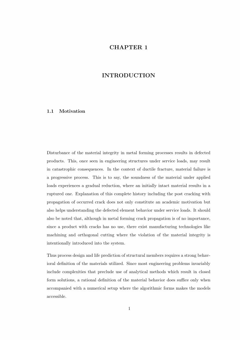
1.1 Motivation
Disturbance of the material integrity in metal forming processes results in defected
products. This, once seen in engineering structures under service loads, may result
in catastrophic consequences. In the context of ductile fracture, material failure is
a progressive process. This is to say, the soundness of the material under applied
loads experiences a gradual reduction, where an initially intact material results in a
ruptured one. Explanation of this complete history including the post cracking with
propagation of occurred crack does not only constitute an academic motivation but
also helps understanding the defected element behavior under service loads. It should
also be noted that, although in metal forming crack propagation is of no importance,
since a product with cracks has no use, there exist manufacturing technologies like
machining and orthogonal cutting where the violation of the material integrity is
intentionally introduced into the system.
Thus process design and life prediction of structural members requires a strong behav-
ioral definition of the materials utilized. Since most engineering problems invariably
include complexities that preclude use of analytical methods which result in closed
form solutions, a rational definition of the material behavior does suffice only when
accompanied with a numerical setup where the algorithmic forms makes the models
accessible.
1

1.2 Aim and Scope
With this motivation, the aim of this study is to present a theoretical and numerical
framework for ductile damage modeling for metal plasticity. The treatment is con-
tent with directional independence in material response which excludes any initial or
deformation induced anisotropy. Besides it does not assume particular restrictions
on the extent of strains. The theoretical side follows principles of thermodynamics,
where purely mechanical (isothermal) and thermo-mechanical derivations are sepa-
rately presented. Formulation of nonlinear isotropic hardening plasticity and com-
bined nonlinear isotropic/linear kinematic hardening plasticity are given. As a post
peak regularizer of the softening response, an over-stress type viscous formulation is
discussed. The presentations are accompanied with intuitive application problems,
involving those with discrete crack formations.
1.3 Modeling Material Weakening
Plasticity and damage are two softening mechanisms that differ on micro-mechanical
foundations. The former entails crystal slip through dislocation movements. The lat-
ter, in the context of ductile damaging materials, requires a progressive deterioration
process, which shows itself in three steps, namely nucleation, growth and coalescence
of micro-voids. Nucleation of micro-voids results in free surface development and
occurs around secondary phase particles or impurities with stress concentrations un-
der plastic flow conditions by particle-matrix debonding, or by inclusion cracking.
Positive hydrostatic stresses cause growth of nucleated and/or already existing micro-
voids to decrease material homogenized stiffness and strength. Under increased loads
the enlarged micro-voids tend to coalesce to form unified macro-crack (failure). This
explains the fact that compressive stress fields promote deformation range whereas tri-
axial stress fields lead premature cracks, see e.g. [149] and [142]. The steps involved
in the deterioration process are illustrated in Figure 1.1. A broad review of governing
mechanisms to give account for material deterioration can be found in [103].
2

Figure 1.1: Progressive deterioration micro-mechanism depending on void nucleation,growth and coalescence.
The failure concept, which can be summarized as the complete loss of load carrying
capacity, has been worked by three different approaches, which are fracture mechanics
(FM), micro-based damage mechanics (MDM) and meso-based damage mechanics (i.e.
continuum damage mechanics (CDM)). For an overview of the methods, the reader is
referred to [24] and the references therein.
1.3.1 FM Models
FM takes into account an accumulated plastic work threshold for material failure.
There are various models proposed in the literature, see e.g. [135] for Oyane cri-
terion, [58] for Freudenthal criterion, [46] for Cockroft Latham criterion and
finally [30] for Brozzo criterion, among others, which are listed in Table 1.1. On the
table, σ represents the Cauchy stress tensor whose maximum principal component is
denoted by σ1. The pressure is given by p. α stands for the rate of equivalent plastic
strain whereas A stands for a material parameter. B1, B2, B3, B4 represent material
dependent fracture thresholds. According to the criteria, once the accumulated plastic
work reaches one of these predefined critical values, fracture occurs.
3
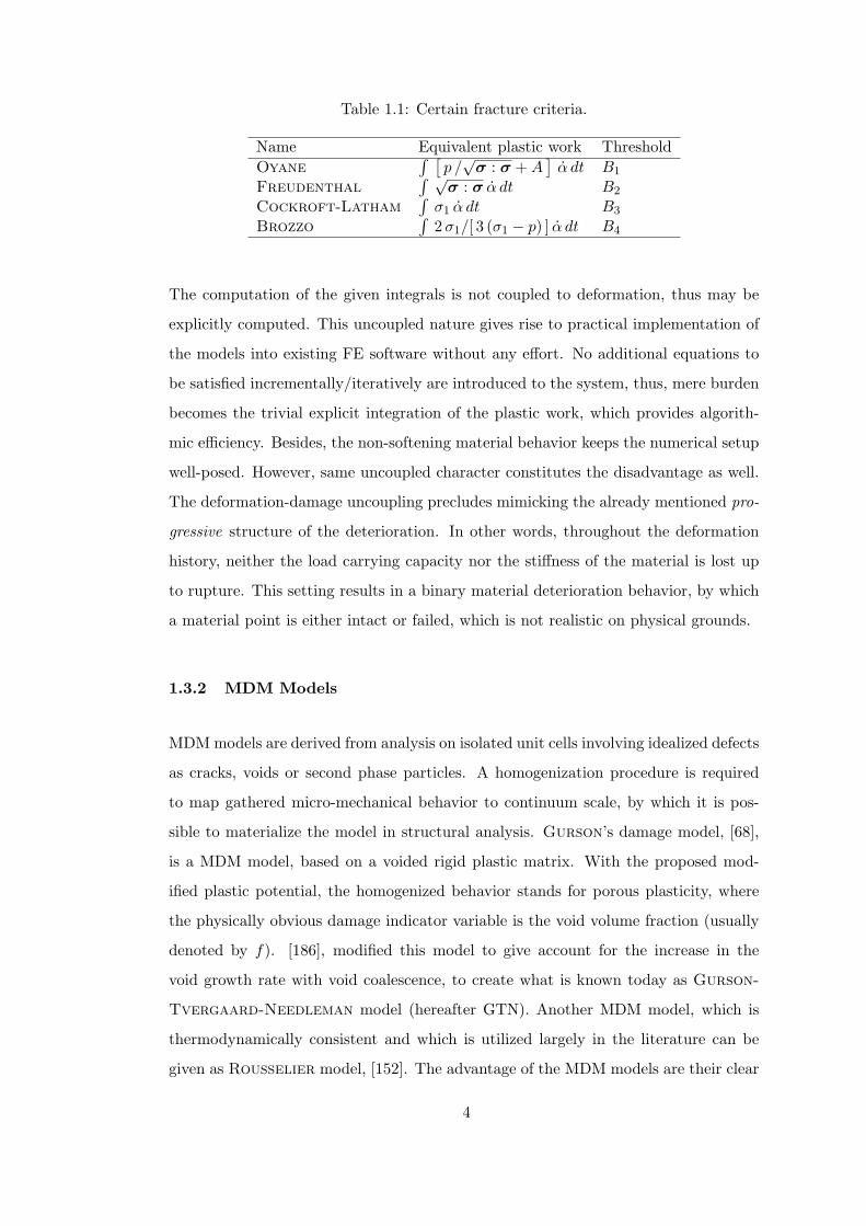
Table 1.1: Certain fracture criteria.
Name Equivalent plastic work ThresholdOyane
∫ [p /√
σ : σ + A]
α dt B1
Freudenthal∫ √
σ : σ α dt B2
Cockroft-Latham∫
σ1 α dt B3
Brozzo∫
2 σ1/[ 3 (σ1 − p) ] α dt B4
The computation of the given integrals is not coupled to deformation, thus may be
explicitly computed. This uncoupled nature gives rise to practical implementation of
the models into existing FE software without any effort. No additional equations to
be satisfied incrementally/iteratively are introduced to the system, thus, mere burden
becomes the trivial explicit integration of the plastic work, which provides algorith-
mic efficiency. Besides, the non-softening material behavior keeps the numerical setup
well-posed. However, same uncoupled character constitutes the disadvantage as well.
The deformation-damage uncoupling precludes mimicking the already mentioned pro-
gressive structure of the deterioration. In other words, throughout the deformation
history, neither the load carrying capacity nor the stiffness of the material is lost up
to rupture. This setting results in a binary material deterioration behavior, by which
a material point is either intact or failed, which is not realistic on physical grounds.
1.3.2 MDM Models
MDM models are derived from analysis on isolated unit cells involving idealized defects
as cracks, voids or second phase particles. A homogenization procedure is required
to map gathered micro-mechanical behavior to continuum scale, by which it is pos-
sible to materialize the model in structural analysis. Gurson’s damage model, [68],
is a MDM model, based on a voided rigid plastic matrix. With the proposed mod-
ified plastic potential, the homogenized behavior stands for porous plasticity, where
the physically obvious damage indicator variable is the void volume fraction (usually
denoted by f). [186], modified this model to give account for the increase in the
void growth rate with void coalescence, to create what is known today as Gurson-
Tvergaard-Needleman model (hereafter GTN). Another MDM model, which is
thermodynamically consistent and which is utilized largely in the literature can be
given as Rousselier model, [152]. The advantage of the MDM models are their clear
4

micro-mechanical motivations reflecting the complete physical phenomena. However,
there are certain disadvantages noted in the literature. The determination of the ma-
terial parameters is impractical 1. Their primarily hydrostatic stress dependent struc-
ture cannot predict shear dominated failure, see e.g. [73]. [64] and more recently [126]
constitute attempts to extent Gurson’s damage model to shear-dominated failure.
Although the shrinkage of the yield locus is reflected which results in the decrease in
load carrying capacity with damage extent, the elastic stiffness degradation in unload-
ing is not captured. Besides, the local conventional setting of MDM formulations give
rise to spurious mesh dependence and nonphysical localization problems in numerical
treatment of the post peak responses. Finally, the micro-mechanical construction of
the formulation constitutes a barrier in transferability of the model to the materials
having different micro-structures.
1.3.3 CDM Models
CDM, which constitutes the main subject matter of this thesis, making use of internal
state variable theory of thermo-mechanics, solves the problem of material weakening
with mathematical phenomenological constructs (i.e. damage variable) which stand
for the internal variables responsible for irreversible micro-structural deterioration.
With its thermodynamic soundness and relative simplicity, the method has been ex-
tensively used to quantify many deterioration types such as elastic, plastic, brittle,
ductile, creep and fatigue, for small and finite strains including directional, thermal
and rate effects. Besides, nonlocal extensions based on integral averaging or gradient
formulations have been proposed to cure the unphysical localization and pathological
mesh dependency of the post peak response, in numerical simulations. The nature of
the approach allows algorithmic treatment in a strain driven framework, which gives
account for a convenient integration into existing nonlinear mechanical solvers, [35].
Such attempts, in the context of isotropic damage coupled finite plasticity, have been
made by [165], [85], [86], [87], [181], [171], [61], [174], [107], [153]; and more recently
with nonlocal extensions by [7], [5] and [116)]. Isotropic damage assumption takes
at hand a randomly and statistically homogeneously distributed, shaped and oriented
1 Calibration of material parameters are relatively easy for three parameter Rousselier damagemodel.
5

micro-void cluster. This postulate of damage isotropy, has proved validity and effi-
ciency for ductile damaging materials. In a general setting, distributed micro-cracks,
i.e. damage, even in a homogeneous and isotropic body create induced anisotropic
and inhomogeneous character of the overall response, [92]. For cases where the pro-
portional loading conditions are violated, anisotropy is favored, [98]. Recently, in the
finite strain context, thermodynamics based anisotropic formulations depending on
multiplicative decomposition of metric transformation tensor are given in [31] and
with nonlocal extensions in [32]. Frameworks with introduction of fictitious undam-
aged configurations are proposed by [117], [53] and [118] to resolve damage induced
anisotropy. Another noteworthy framework, treating anisotropic (visco)damage cou-
pled with (visco)plasticity and its nonlocal extensions can be found in [2] and [189],
respectively. Recently, proposing functional forms for inelastic hardening variables in
damage and plasticity, [190] resolves the coupled problem including directional effects.
The advantage of CDM is the existence of consistent derivation through thermody-
namics of irreversible processes. Besides, these models are capable to reflect both
the shrinkage of the admissible stress space and the elastic stiffness degradation with
material deterioration. Like in the case of MDM models, this softening behavior in
turn creates an ill-posed initial boundary value problem, with the loss of ellipticity
for quasi-static cases, and loss of hyperbolicity for dynamic problems, where spuri-
ous mesh dependence and nonphysical localization problems are due for post peak
responses.
The literature on CDM has reached to a mature level. Reader may refer to the texts
of [98], [92], [169], and [99]. Additional references having chapters on the subject are
[97], [50], [38] and [154].
1.3.3.1 Fundamental Hypotheses of Utilized Phenomenological Damage
Models
In the current presentation, the formulations are based on the concept of effective
stress and the principle of strain equivalence. In order to illustrate these members
of the foundation, a geometrical insight into the meaning of the damage variable is
possible by considering a one dimensional tensile test specimen which is represented
6

in two spaces one of which is physical and the other is fictitious, as given in Figure
1.2. Physical space stands for the actual case where the effect of micro-cracks and
micro-voids persist, whereas the fictitious space is assumed to be defect-free.
Figure 1.2: Effective stress concept.
Considering the cross section of the specimen, the nominal area, which takes place in
the physical space, is represented by A, and the defect-free area, which takes place
in the effective space, is represented by A. Once the damaged area, AD = A − A, is
scaled with A, one reaches an objective measure for damage, which verbally stands
for the ratio of the damaged area to the total area, at the plane of interest,
D =AD
A
with D ∈ [0, 1], where the lower bound, D = 0, represents the intact material without
any damage, and the upper bound, D = 1, represents complete rupture2.
2 A noteworthy point is that, although CDM provides a strong coupling environment where theprogressive deterioration of the material is resolved, for high strength and low ductility materials(like high carbon steels), critical damage values (which denotes the local material failure) can beconsiderably small (Dcr can even be in the order of 0.05, see e.g. [188]. The micro-mechanical pictureis in correlation to this fact, the critical void volume fraction for element failure is taken as f = 0.05to f = 0.2, where f = 1.0 is never practically reached, [61]). This may lead to a FM-like uncoupledapplication. However, the model produced should be applicable to larger extent of materials togetherwith less mathematical restrictions and provide soundness on physical grounds. Thus, in this studya fully coupled progressive deterioration mechanism is presented in chevron prediction.
7

The Cauchy stress acting in the physical space is named as the nominal stress,
whereas the effective Cauchy stress, σ, acts at the undefected material sub-scale, i.e.
in the effective space. This phenomenological approach has the roots from the works
of [88] and [144], where the creep rupture in metals is considered.
Once nominal-effective separation is introduced to the field variables, the construction
of the constitutive setup in between dual forms constitutes the central problem. For
this purpose, in the literature, certain equivalence principles, such as strain equiva-
lence, stress equivalence and energy equivalence, are proposed. These have certain
advantages and disadvantages over each-other, investigation of which is beyond the
aim of the current work3. The strain equivalence principle, [95], as illustrated in Fig-
ure 1.3, states the equivalence of the strain under actual nominal stresses with the
strain computed at the fictitious undamaged state under effective stresses. In other
words, it assumes the validity of canonical constitutive forms, once the stress measure
is selected in terms of the effective one.
Figure 1.3: Principle of strain equivalence.
3 We content with noting that, the principle of energy equivalence is especially utilized togetherwith anisotropic damage modeling.
8

1.4 Organization of the Thesis
The thesis is organized in the form of a collection of the following self-contained
chapters,
In Chapter 2, a local, isotropic damage coupled hyperelastic-plastic framework is for-
mulated in principal axes using an eigenbases representation. It is shown that, in a
functional setting, treatment of many damage growth models, including ones orig-
inated from phenomenological models (with formal thermodynamical derivations),
micro-mechanics or fracture criteria, proposed in the literature, is possible. Quasi-
unilateral damage evolutionary forms are given with special emphasis on the fea-
sibility of formulations in principal axes. Moreover local integration procedures are
summarized starting from a full equation set which are simplified step by step initially
to two and finally to one. Also different operator split methodologies such as elas-
tic predictor-plastic/damage corrector (simultaneous plastic-damage solution scheme)
and elastic predictor-plastic corrector-damage deteriorator (staggered plastic-damage
solution scheme) are given. Besides possible extensions to involve linear kinematic
hardening are formulated in a thermodynamically consistent manner. To this end
regarding consistent material moduli are derived. The model is implemented as a user
defined material subroutine UMAT for ABAQUS/Standard and UFINITE MSC.Marc and
tested for a set of sample problems evaluating the accuracy and predictive capabilities
of the developed algorithms in a purely mechanical setting.
In Chapter 3, a thermo-mechanical framework for damage-coupled finite (visco) plas-
ticity with nonlinear isotropic hardening is presented in an eigenvalue representation.
The formulation makes use of the internal variable theory of thermodynamics and,
following in the footsteps of [162], introduces inelastic entropy as an additional state
variable. It is shown that, given a temperature dependent damage dissipation po-
tential, the evolution of inelastic entropy assumes a split form relating to plastic and
damage portions, respectively. For regularization of the doubly induced softening due
to damage and temperature, a simple Perzyna type viscosity is devised. Analyti-
cal forms, which provide an account of the effect of damage on heat conduction, and
provide a thermo-mechanical framework accompanied by algorithmic forms for a stag-
gered scheme based on the so-called isothermal split, are derived. A possible setting
9

for the adiabatic formulation is also presented. The model is implemented as UMAT
and UMATHT subroutines for ABAQUS/Standard and used in a set of application prob-
lems, among which, two novel necking triggering methods (similar to the thermal and
geometric imperfection methods) are introduced in the context of a damage coupled
environment.
In Chapter 4, materializing Continuum Damage Mechanics (CDM), numerical model-
ing of discrete internal cracks, namely central bursts, in direct forward extrusion pro-
cess is presented. For this purpose, a thermodynamically consistent Lemaitre-variant
damage model with quasi-unilateral evolution which is coupled with hyperelastic-
plasticity is utilized. With VUMAT subroutine combined with an element deletion
method and with a UMAT subroutine combined with an appropriately implemented
ramped element degradation method, the model is used in the simulation of central
crack formations in forward extrusion of 100Cr6 with single reduction and Cf53 with
double reduction, using explicit and implicit FE schemes, respectively. On the physi-
cal side, relative predictive performances are observed. The investigations reveal that,
in application of the quasi-unilateral conditions, the crack closure parameter has an
indispensable effect on the damage accumulation zones by determining their internal
or superficial character. Combining a suitably selected crack closure parameter with
the element deletion procedure, discrete cracks are obtained. The periodicity of the
cracks shows well accordance with the experimental facts. Besides, investigations on
the effect of many process parameters on the final distribution of mechanical fields are
presented. Moreover, it is demonstrated that, application of counter pressure intro-
duces a marked decrease in the central damage accumulation, which in turn increases
the formability of the material through keeping the tensile triaxiality in tolerable lim-
its. It is also shown that, for a crack involving process, through systematic increase
of the counter pressure, the crack sizes diminish; where at a certain level of counter
pressure chevron cracks can be completely avoided.
Finally, Chapter 5 shortly summarizes the thesis work and addresses the future per-
spectives.
10

1.5 A Word on Notation
Throughout the thesis, following notations will be used. Assuming a, b, and c as three
second order tensors, together with the Einstein’s summation convention on repeated
indices, c = a • b represents the product with [c]ik = [a]ij [b]jk. d = a : b represents
the inner product with d = [a]ij [b]ij where d is a scalar. E = a ⊗ b, F = a⊕ b and
G = a b represent the tensor products with [E]ijkl=[a]ij [b]kl, [F]ijkl=[a]ik[b]jl and
[G]ijkl=[a]il[b]jk, where E, F and G represent fourth order tensors. [F]t and [F]−1
denote the transpose and the inverse of [F], respectively. DIV[F], GRAD[F] and
div[F], grad[F] respectively designate the divergence and gradient operators with re-
spect to the coordinates in the reference and current configurations. [F]sym and [F]skw
are associated with the symmetric and skew-symmetric parts of [F] respectively, with
[F] = [F]sym + [F]skw.
11

CHAPTER 2
ISOTHERMAL FORMULATION
2.1 Introduction
The purpose of this Chapter is to present, in an Euclidean setting, a sound finite
strain hyperelastic-plastic framework coupled with local isotropic damage, formulated
in the principal axes. For this purpose, using the concepts of effective stress, [88]
and [144], and principle of strain equivalence, [95], a strongly coupled plasticity and
damage formulation is followed through a single yield function. With this, damage
occurrence is strictly accompanied by plastic flow which is realistic for ductile damage.
The computational features of the current framework that are worth mentioning can
be listed as follows:
• Presented framework in principal axes provides convenience in formulation of
the damage coupled finite hyperelastic-plasticity reducing the tensorial differen-
tials to simple scalar differentials, [80]. This simplicity is especially apparent in
consistent linearization of the problem,
• The principal axes representation of the damage (pseudo)conjugate variable can
readily be extended to give account for the formulation of the active-passive
conditions, which serves handiness compared to tensorial representations,
• There are no particular restrictions on the forms of the governing functions of
plasticity in terms of nonlinear isotropic hardening,
• With the proposed functional setting, there are also no particular restrictions
on the damage evolutionary forms as well. Possible forms, that can be treated
12

in this setting, include damage models derived from various damage dissipation
potentials. Besides, exploiting the proportionality of the plastic multiplier and
the equivalent plastic strain rate for a class of plasticity models, without violat-
ing the second principle of thermodynamics, it is possible to expand the existing
set of damage models together with a broad range of possible progressive dete-
rioration formulations, including fracture criteria based and micro-mechanically
based ones.
• The complete numerical setting is constructed on eigen-bases rather then eigen-
vectors, which is more efficient, as far as especially the fourth order tangent
moduli computations are concerned, [119].
• The local integration schemes, which results in different operator-split method-
ologies such as elastic predictor-plastic/damage corrector type (simultaneous
plastic/damage solution scheme) and elastic predictor-plastic corrector-damage
deteriorator type (staggered plastic/damage solution scheme), are thoroughly
presented. These schemes are supported with systematic reductions applied to
the total number of governing equations at the local stress update problem.
This chapter has the following outline. Local constitutive forms are derived in § 2.2
in a thermodynamic consistency and a functional damage rate form, which unifies
the ductile damage models utilized in the literature, is proposed. In § 2.2.3, a model
problem with J2 plasticity and a Lemaitre variant damage model is presented to-
gether with unilateral damage evolutionary forms formulated in principal stress space.
Numerical aspects, including the algorithmic forms and the consistent tangent moduli
are given in § 3.3. The example problems take place in § 2.4.
2.2 Theory
2.2.1 Multiplicative Factorization
With reference to Figure 2.1, let x ∈R3 and X ∈R3designate the positions of the
particle in the current configuration, B ⊂ R3, and the reference configuration, ϕ(B) ⊂
R3, respectively. F is the deformation gradient via F =∂Xx. The motion ϕ(X, t) :
13

B× R → R3 is responsible for the mapping x = ϕ(X, t).
Figure 2.1: Description of motion and configurations.
The multiplicative framework, according to the kinematics of [94], is micro-mechanically
justified in [11] for single crystals, where the same setup preserves validity for the
use together with the macroscopic phenomenological theory of polycrystalline media
due to similarity of deformation mechanisms between single and polycrystals, [140].
Multiplicative kinematics postulates the local multiplicative decomposition of the de-
formation gradient into elastic and plastic portions as 1,
F = Fe • Fp. (2.1)
The illustration of this decomposition, together with valid Eulerian and Lagrangian
strain measures is given in Figure 2.2. The local character of this factorization is re-
flected by the circles which represent the neighborhood of the regarding placements.
1 Arguments on the non-uniqueness of this decomposition, stemming from the arbitrariness ofthe intermediate configuration, can be found in e.g. [50, p. 398], [106, pp. 455–456] and [163, pp.337–338] among others. The definition of proper state variables to give account for an appropriatefinite strain multiplicative framework, supplying the invariance requirement, is a rather much debatedissue and it is beyond the scope of the current study. Here, merely, the exploitation of [163, pp. 337–338] is followed. Accordingly, together with the isotropy condition the orientation of the intermediateconfiguration is irrelevant. Thus the non-uniqueness of the decomposition does not arise as a problemin this context and does not affect the derivations once the stored energy is constructed in terms ofbe. A recent investigation on the internal dissipation inequalities for finite strain constitutive lawstogether with their theoretical and numerical consequences is given in [102].
14

Figure 2.2: Multiplicative kinematics of Lee.
For numerical modeling of this formulation, to give account for finite strain elasto-
plastic formulation, see e.g. [158], [159], [161] and [164] among others. The principal
axes formulation of finite (visco)plasticity, in manifold and Euclidean settings2, can
be found in [79], [80], [81] and the references therein.
2.2.2 Thermodynamic Framework
In coupling isotropic damage with plasticity using multiplicative kinematics, it is
started with the definition of free energy potentials, where isotropic hardening plastic-
ity is taken into account only. Expansion of the current setting to kinematic hardening
is given in the following pages. Merging the finite strain plasticity framework of [163]
and thermodynamics of internal variables, [98], in definition of damage including pro-
cesses, an additively decoupled total free energy, Ψ, in terms of elastic and isotropic
hardening plastic portions, i.e. Ψe and Ψp,iso, respectively, is selected as follows,
Ψ(be, α,D) = Ψe(be, D) + Ψp,iso(α), with Ψe(be, D) = (1−D) Ψe(be). (2.2)
In Equation 2.2, be and α denote the elastic left Cauchy-Green deformation tensor
and the isotropic hardening (strain like) internal variable, respectively. D ∈ [0, 1],
2 Advantage of a manifold formalism, together with a coordinate free representation, where theframework is equipped with a metric, is obvious (e.g. for space curved membranes and shells). Eu-clidean setting, where 3D, 2D plane stress, plane strain and axi-symmetric formulations of continuumare due, constitutes a particular choice of coordinate representation where the metric boils down to aunit tensor.
15

represents the isotropic damage variable and has a clear geometrical definition as the
damaged area density at the plane of attention, [88]. Effective elastic potential, i.e.
Ψe(be), is the free elastic energy of the fictitious undamaged continuum. In this setting
damage is coupled to elasticity with state coupling.
In pure local mechanical form, a non-negative dissipation, which is the difference
between the local stress power and the local rate of change of free energy, according
to the second principle of thermodynamics, can be set as follows,
Ω = τ : d− ∂tΨe + ∂tΨp,iso︸ ︷︷ ︸=∂tΨ
≥ 0, (2.3)
with ∂t [F] := ∂ [F] /∂t, and d := sym [l] representing the rate of deformation tensor
which is the work conjugate of the Kirchhoff stress tensor, where l := ∂tF • F−1
denotes the spatial velocity gradient. (2.3) gives the state equations between dual
variables, after proper modifications,
τ = 2 (1−D) ∂beΨe • be, (2.4)
q = −∂αΨ = −∂αΨp,iso, (2.5)
Y d = −∂DΨ = Ψe. (2.6)
where, q is responsible for isotropic hardening, in the form of yield locus expansion,
and Y d is the thermodynamically formal damage conjugate variable, in the form of
the elastic strain energy energy release rate. This form is in accordance with the
canonical Lemaitre damage model. Using the effective Kirchhoff stress definition
as, τ = τ/(1−D), it is seen that, due to the strain equivalence principle, the effective
stresses do not depend explicitly on D. Substituting (2.4), (2.5) and (2.6) in (2.3),
the following dissipation potential expression is carried out,
Ω = −τ : [12£vbe • be,−1] + [−∂αΨp,iso]︸ ︷︷ ︸
=:q
∂tα + [−∂DΨ]︸ ︷︷ ︸=:Y d
∂tD, (2.7)
where £v [F] stands for the objective Lie derivative of [F], [109]. The evolutionary
forms are defined postulating a combined loading function, in an additively decoupled
combination of the plastic potential, i.e. φ, and a damage dissipation potential, i.e.
φd,
φt(τ, q, Y d;α, D) = φ(τ , q) + φd(Y d;α, D). (2.8)
16

The plastic flow is physically possible at undamaged material sub-scale, which corre-
sponds to the formulation of φ in the effective Kirchhoff stress space. Following the
hypothesis of generalized standard materials, which proposes the existence of normal-
ity rules, [111], one derives the plastic flow rule and the rate expressions for α and D
as,
£vbe = −2γ
(1−D)∂τ φ • be, (2.9)
∂tα = γ ∂qφ, (2.10)
∂tD = γ ∂Y dφd, (2.11)
which are conventional, associative evolutionary rules. In the following, plastic isotropic
hardening and many damage softening forms are unified within respective functional
settings.
2.2.2.1 Functional Isotropic Hardening Forms
Selection of the form for the plastic potential will naturally yield a set of state equa-
tions for isotropic hardening plasticity. For (2.5), a generalized function, K ′ (α) :=
−∂αΨp,iso with q = K ′ (α), can be defined using various forms proposed in the
literature as given in Table 2.1.
Table 2.1: Plasticity isotropic hardening models in the functional setting.
ID Name K ′ (α)A. Linear K αB. Saturation K α + (τ∞ − τ0) (1− exp [−δ α])C. Swift τ0 [(c + α)− 1]D. Ramberg-Osgood K αn
E. Logarithmic τ0 [ ln (c + α)− 1]
On the table, K stands for the linear hardening parameter, whereas τ0 and τ∞ repre-
sent yield stress and saturation stress, respectively. δ and c constitute other material
constants.
17

2.2.2.2 Functional Damage Rate Forms
Following thermodynamics of internal variables, and using the effective stress concept,
strain equivalence principle, state coupling with elasticity and kinematic coupling with
plasticity, different isotropic damage evolutionary models can be postulated propos-
ing different damage dissipation potentials, i.e. φd. Eventual integration of the de-
rived rate forms supplies diverse patterns for damage curves with increasing plastic
strain. Together with proposing an exponential ductile continuum damage model, [39]
presents a comparative study showing relative performances of some damage models
utilized in literature. The models such as Lemaitre damage model, [96], Tai’s dam-
age model, [182], Chandrakanth and Pandey’s damage model, [39] and [40], are
capable of reflecting concave-up type damage evolution with plastic strain. On the
other hand, there are more general damage models, by taking into account the de-
pendence of damage dissipation potential on equivalent plastic strains, give rise to a
potential of mimicking a larger range of nonlinear damage evolutionary forms, ranging
from concave-down to concave-up. The model of Tie-Jun, [184], and the model of
Bonora, [23], later validated in [24] for low alloy steels under various triaxialities
and in [25] for ferritic steels, are of this kind. [23] shows that for Al2024 and Al-
Li alloys, where the damage evolution rate is dominated by the nucleation process,
which includes nucleation of multiple voids, damage accumulation patterns other than
concave-up are observed.
Derivation of a dissipation potential may not seem to be an easy task. Without for-
mally tracking the scheme given in § 2.2.2, a consistent definition of damage rate,
which does not violate the Clausius Duhem inequality, is possible (i.e. no damage
healing, D > 0). This gives rise to a broad range of progressive damage evolution-
ary forms such as the three invariant damage model, given in [97], also used in [155]
for chevron predictions in cold axi-symmetric extrusion or those based on fracture
criteria or some micro-mechanical damage models. An example for the fracture cri-
teria based CDM model may be given as the triaxiality dependent damage model of
[63], also used in [116)], which proposes the progressive deterioration counterpart of
the Oyane’s ductile fracture criterion originally proposed in [136]. For this class of
models, as progressive counterparts of accumulated plastic work dependent models,
18

it is possible to exploit Freudenthal criterion, [58], Cockroft Latham criterion,
[46], or Brozzo criterion, [30]. The phenomenological CDM version of the micro-
mechanically based void growth model of [149], given in [65] and also used in [51],
constitutes an example for the micro-mechanically based CDM model.
The possibility of collecting the mentioned damage forms in a unified framework,
together with a functional setting, suitable for the current finite plasticity in principal
axes, forms the main motivation of this section. This has the apparent advantage of
robust implementation of a user defined material routine for a broad range of damage
models with minimum effort.
To set the stage, in the internal variable setting, damage growth models are postulated
to have the following generalized functional form, without specifying any particular
damage potential, i.e. φd,
D = f(τ ; ξ, D), (2.12)
where ξ represents the vector of hardening internal variables (possibly together with
their rates) in the form of scalars/tensors (e.g. isotropic/kinematic hardening vari-
ables respectively). In the present strong plastic-damage coupled environment, in the
absence of kinematic hardening, following modification of (2.12) holds, making use of
the proportionality of γ and α,
D = γ g(Y ;α, D), with Y = Y (τ). (2.13)
Additional function Y may seem superfluous, however the form (2.13) is proposed
to catch an accordance with the thermodynamically formally derived damage rate
form given in (2.11), together with g = ∂Y dφd/∂qφ, and Y = Y d. Hence (2.13)
covers all thermodynamically consistent damage models where φd = φd(Y d;α, D),
including those mentioned at the beginning of the section. Moveover, (2.13) may
emerge as many functional forms in Y , where Y , an isotropic function of τ3, is not
necessarily a formal damage work conjugate variable4. Table 2.2 lists some of the
damage growth rules used in the literature in the context of ductile damage mentioned
in the previous paragraphs, which are modified to fit (2.13), in the current finite strain
framework. Model E constitutes a generalization of the model proposed in [65]. The3 Thus, Y can be represented in terms of principal stresses, i.e. τ1, τ2, τ3, and it is feasible to be
tackled in a principal axes formulation.4 Y , where Y 6= −∂DΩ, is named as damage pseudo-conjugate variable.
19

components p, τ1 and τeq represent the effective Kirchhoff type pressure, maximum
principal Kirchhoff stress and equivalent von Mises stress respectively. All the
other variables except for Y , α and D refer to the appropriate material parameters
defined in the original references.
2.2.3 Application to A Model Problem
2.2.3.1 Spectral Representations
Starting with, the link between the tensorial forms and the principal values are con-
structed through the following spectral decompositions,
be =3∑
A=1
beA mA, εe =
3∑A=1
εeA mA, τ =
3∑A=1
τA mA, s =3∑
A=1
sA mA, (2.14)
where εe denotes the elastic logarithmic strain tensor and s represents the deviatoric
Kirchhoff stress tensor together with the respective eigenvalues (principal values) as
εeA and sA. Thanks to isotropy, among the tensors given in (2.14), identical eigen-bases,
i.e. mA = νA ⊗ νA, are shared, where νA represents the corresponding eigenvectors
with (A = 1, 2, 3). The principal values of the logarithmic elastic strains are defined in
terms of elastic principal stretches, i.e. λeA, as, εe
A = log[λeA]. The deviatoric portion
of λeA =
√beA and εe
A are represented by λeA and εe
A. respectively.
In what follows, the presented framework is specialized for a specific model including a
hyperelastic potential quadratic in logarithmic elastic strains represented by principal
stretches, von Mises plasticity represented in principal effective stress space and a
quasi-unilaterally evolving Lemaitre variant damage model. Initially the derivations
are made for mere isotropic hardening plasticity. Formulations for kinematic hardening
follow for the sake of completeness.
20

Tab
le2.
2:D
amag
em
odel
sin
the
func
tion
alse
ttin
g.
IDR
efer
ence
g=
g(Y
;α,D
)Y
=Y
(τ)
A.
Lemait
re
(198
5)(Y
/S0)s
Yd(τ
)
B.
Lemait
re
and
Chaboche
(199
0)(Y
/S0)s
/(1−
D)b
α1〈p〉+
α2〈τ
1〉+
(1−
α1−
α2)τ
eq
C.
Tai(1
990)
D(Y
/S0)
Yd(τ
)
D.
Tie
-Jun
(199
0)(Y
/S0)1
/[(
1−
α/α
cr)(
1−
b)α
(2/n) ]
Yd(τ
)
E.
Gunawardena
etal
.(19
91)
(m1+
m2D
)ex
p[(3
/2)Y
]〈p
/τ e
q〉
F.
Chandrakanth
and
Pandey
(199
3)(Y
/S0)[
1/(1−
D)n−
(1−
D)]
Yd(τ
)
G.
Dhar
etal
.(1
996)
a0+
(a1+
a2D
)YS/(1−
D)q
Yd(τ
)
H.
Bonora
(199
7)(Y
/S0)(
Dcr−
D)(
q−
1/q) /
[(1−
D)α
(2+
n)/
n]
Yd(τ
)
I.G
oijaerts
etal
.(20
01)
〈1+
aY〉α
p/τ e
q
21

2.2.3.2 Free Energies and Regarding State Laws
For isothermal conditions, one postulates the following deviatoric volumetric split for
the effective elastic potential,
Ψe(be) := Ψe,vol(Je) + Ψe,dev(λeA), (A = 1, 2, 3), (2.15)
where the frame invariance lets one use the principals of the tensor arguments in
representation of the isotropic functions,
Ψe,vol(Je) :=12
H log[Je]2, (2.16)
Ψe,dev(λeA) := µ (log[λe
1]2 + log[λe
2]2 + log[λe
3]2)
= µ (εe,21 + εe,2
2 + εe,23 ). (2.17)
This quadratic form, although preserves validity for a large class of materials up
to moderately large deformations [3], [4], does not satisfy the polyconvexity condition
[102]. For the plastic portion, following isotropic hardening potential is common which
is associated with the combined linear and saturation type hardening,
Ψp,iso(α) :=12K α2 + (K∞ −K0) (δ + exp[−δα]/δ). (2.18)
Accordingly, one finds the following state equation for τ ,
τ = (1−D)[Htr[ε e]︸ ︷︷ ︸=:p
1 + 2µ εe︸ ︷︷ ︸=:s
], (2.19)
where p = (τ1 + τ2 + τ3)/3. One also may derive,
q = K α + (K∞ −K0) (1− exp[−δα]), (2.20)
Y d = Ψe,vol(Je) + Ψe,dev(λeA). (2.21)
2.2.3.3 Dissipation Potentials and Regarding Evolutionary Forms
The definition of the yield potential, which is of von Mises type, is made in the
effective Kirchhoff stress space in terms of the principal values of the effective
Kirchhoff stresses, as,
φ(τA, q) :=
√23
(τ21 + τ2
2 + τ23 − τ1 τ2 − τ1 τ3 − τ2 τ3)
12 −
√23
y(q) ≤ 0, (2.22)
22

where y(q) = (τ0 + q) represents the hardening/softening function for isothermal
conditions, and τ0 is the initial yield stress of the virgin material. Using this weakly5
coupled potential, the expressions for ∂τ φ and ∂qφ, taking place in (2.9) and (2.10)
respectively, can be derived as follows,
∂τ φ =3∑
A=1
nA νA ⊗ νA ⇒ £vbe = −2γ
(1−D)(
3∑A=1
nA νA ⊗ νA) • be, (2.23)
∂qφ =
√23
⇒ ∂tα = γ
√23, (2.24)
where nA = ∂τA φ = sA/ 2√
s21 + s2
2 + s23. Pay attention to the fact that the eigen-bases
for the effective and the homogenized stresses are equivalent, i.e. mA = νA ⊗ νA ≡
mA = νA ⊗ νA.
2.2.3.4 A Lemaitre Variant Damage Model
For the damage evolutionary form, preserving generality g(Y ;α, D) with Y = Y d, i.e.
the formal damage conjugate variable defined in (2.6), is selected, as in the case of
Lemaitre damage model. (2.21), which is given in elastic logarithmic strains, can be
reformulated in the effective principal Kirchhoff stress space together with (2.19),
to give Y d(τA), (A = 1, 2, 3) as follows,
Y d(τA) =1 + ν
2E(τ2
1 + τ22 + τ2
3 )− ν
2E(τ1 + τ2 + τ3)2, (2.25)
or shortly
Y d(τA) =1 + ν
2E(τ2
1 + τ22 + τ2
3 )− 9ν
2Ep2, (2.26)
where p = (τ1 + τ2 + τ3)/3. This form involves the effect of triaxiality intrinsically as
follows
Y d =τ2eq Rv
2E, (2.27)
where Rv is the triaxiality function,
Rv =23
(1 + ν) + 3 (1− 2ν)(
p
τeq
), (2.28)
5 Here, weakly coupled refers to no hardening-damage coupling, where merely the effective stresscontributions take place in the yield function but not the effective counterparts of the hardeningvariables, [20]. The plasticity-damage coupling is referred to as strong on the other hand due to theuse of a single plastic potential coupled to damage, restricting damage by not allowing its growthwithout accompanying plastic flow. Comparison of possible coupling mechanisms can be found in[107].
23

and τeq is the equivalent von Mises stress which is defined in terms of principal
components as τeq = (τ21 + τ2
2 + τ23 − τ1 τ2 − τ1 τ3 − τ2 τ3)1/2.
Remark 2.2.1 In the original Lemaitre damage model, the conjugate damage force,
Y d, is defined as, [98]
Y d =1 + ν
2E(1−D)2τ : τ − ν
2E(1−D)2tr[τ ]2,
which is identical to (2.25) with the effective stress definition.
2.2.3.5 Quasi-Unilateral Damage Evolution
Physical facts show that, the damage evolution is amplified in tensile conditions
whereas under compressive loads the rates of deterioration dramatically reduce. This
is due to the partial micro-crack closure. Accordingly, quasi-unilateral damage takes
into account evolution fully in tension and partially (or none) in compression. For a
3D stress state, the tensile and the compressive characters of the tensor components
may not be apparent. For this purpose, two common resolutions are due.
The former, being a rather simplistic approach, proposed in [178] and [141] where
the damage accumulation rate for cyclic plasticity is analyzed, relies on the character
of the triaxiality (or equivalently the hydrostatic stress component). Hence, damage
accumulates under positive (tensile) hydrostatic stresses where the damaged mate-
rial stiffness is utilized. For negative triaxialities on the other hand, neither damage
accumulates (not even partially), nor a reduction in the tangent is given account for.
In the latter more rigorous method, decision is made using the distinct principal ten-
sor (stress or strain) components. Accordingly, the tensile and compressive principal
tensor components are sought, where, for the extraction of these components, use of
projection operators are proposed, see, e.g. [104] and [92], as well as spectral decom-
positions, see, e.g. [199]. In view of that, the damage conjugate variable definitions
are refined to support quasi-lateral damage evolutionary forms, fully contributed by
tensile stresses and partially contributed by compressive stresses, parameterized by
the crack closure parameter.
Two methods have relative advantages and disadvantages. The form given in [178] and
24

[141] is very efficient and supplies rapid qualification of the evolutionary conditions.
Besides, it does not require a crack closure parameter. However, this simplicity may be
seen as a drawback of the method, where there is no space for partial damage evolution
under compressive hydrostatic stresses. As far as the void nucleation with shear
decohesion under compressive stresses is taken into account, this requirement may be
seen over-restrictive. The principal stress/strain projection method on the other hand
intrinsically takes into account these mechanisms to a certain level governed by the
crack closure parameter. However, the method results in a more complicated algorithm
as far as the computation of the evolutionary forms and the material tangents are
concerned.
The advantage of the current framework using the principal stress space formulation
comes to scene at this stage with its ease of application of the quasi-unilateral dam-
age evolutionary forms (i.e. active/passive damage evolutionary conditions). Since
the existing formulation is already a principal axes one, it is naturally devised for
the active/passive conditions, thus does not necessitate an additional labor for ex-
tracting the principal tensile and principal compressive portions of stress tensors with
projection operators or spectral decompositions. Accordingly, one may propose the
following refined damage conjugate variable to give account for the quasi-lateral dam-
age evolution, with fully contributed by tensile stresses and partially contributed by
compressive stresses as,
Y d,+(τA) =1 + ν
2E(〈τ1〉2 + 〈τ2〉2 + 〈τ3〉2)−
9ν
2E〈p〉2
+h (1 + ν)
2E(〈−τ1〉2 + 〈−τ2〉2 + 〈−τ3〉2)−
9h ν
2E〈−p〉2,
(2.29)
where 〈F〉 is the Macauley bracket with 〈F〉 := 1/2 (F + |F|) and h ∈ [0, 1] is
the crack closure parameter. The two extremes where h = 0 and h = 1 correspond
to complete and no crack closure respectively, where for steels h is generally taken
as 0.2, [98]. The use of effective principal Kirchhoff stresses highly simplifies not
only the form of the expressions, but also the consequent derivations. This apparent
simplicity is applicable to all of the isotropic damage models given in Table 2.2, where
Y (τ) is reformulated as Y (τA) with (A = 1, 2, 3) . In the current framework, unlike
[99, p. 105], identical damage independent effective stress definition for elasticity and
plasticity is used.
25

Application of the quasi-unilateral conditions with anisotropic damage is prone to
certain anomalies, which is beyond the purpose of the current study. For a general
perspective, the reader is referred to [38] and the references therein.
2.2.4 Expansion to Kinematic Hardening
Inclusion of kinematic hardening is made in the simplest manner by introducing an
additional term to the plastic free energy in (2.2). Accordingly, an additively decou-
pled form into isotropic, i.e. Ψp,iso, and kinematic, i.e. Ψp,kin, portions are assumed,
such as,
Ψp(α, z) = Ψp,iso(α) + Ψp,kin(z), (2.30)
where an additional dissipation term due to the kinematic hardening, Ωp,kin, is added
to the pure local mechanical inequality,
Ω = τ : [−12£vbe • be,−1] + Ωp,kin(z) + q ∂tα + Y d ∂tD ≥ 0, (2.31)
with z and β being kinematic hardening strain-like and stress-like variables, respec-
tively. β is also called the backstress, associated with the center of the yield surface,
i.e. elastic range. Geometrical interpretation of the isotropic, kinematic and combined
isotropic/kinematic hardening models are respectively given in Figure 2.3.a, Figure
2.3.b and Figure 2.3.c in the Π plane, defined at the effective Kirchhoff stress space,
for an initially virgin yield locus, given by the dashed circles. More complicated hard-
ening models can be developed by distorting the locus by accompanied plastic flow.
For kinematic hardening, in the context of multiplicative kinematics, two possible
approaches that are proposed in the literature, which are named as Model A and
Model B, are utilized. Model A is due to [81] and Model B is due to [102], where the
details are in Table 2.3.
26

Figure 2.3: Yield locus evolution in Π plane, a) Isotropic hardening, b) Kinematichardening, c) Combined isotropic/kinematic hardening.
Table 2.3: Utilized kinematic hardening models.
Expression Model A Model Bβ 2∂zΨ • z ∂zΨ
Ωp,kin β :[−1
2£vz • z−1]
β :[−4ξ
]Objective rate £vz = z− l • z− z • lt
4z =
3∑A=1
zA νA ⊗ νA
In both of the formulations, it is hypothesed that, be is coaxial with z, (equivalently,
so are τ and β). Also z and β are deviatoric and symmetric tensors. Accordingly
following expressions are valid,
z =3∑
A=1
zA νA ⊗ νA; zA = γ2A, (2.32)
β =3∑
A=1
βA νA ⊗ νA. (2.33)
In Model A, the form of the Kirchhoff type kinematic hardening stress like variable is
analogous to the Kirchhoff stress definition. The dissipation potential is constructed
in terms of Lie derivative of z. This form is direct extension of the dissipation potential
to give account for damage derived in the reference configuration in [81], as,
0 ≤ Ω := −S :12C • ∂tGp •Gp,−1 −A :
12C • ∂tΞ •Ξ−1 + q ∂tα + Y d ∂tD, (2.34)
27

where z = F •Ξ • Ft, β = F •A • Ft, be = F •Gp • Ft. Accordingly one finds
∂tbe − l • be−be • lt︸ ︷︷ ︸=:£vbe
= F • ∂tGp • Ft, (2.35)
∂tz− l • z− z • lt︸ ︷︷ ︸=:£vz
= F • ∂tΞ • Ft. (2.36)
Except for the trivial case of q ∂tα ≡ q ∂tα, Y d ∂tD ≡ Y d ∂tD, for scalars, one can
derive the following equivalences to complete the case,
−S :12C • ∂tGp •Gp,−1 ≡ τ : [−1
2£vbe • be,−1], (2.37)
−A :12C • ∂tΞ •Ξ−1 ≡ β :
[−1
2£vz • z−1
], (2.38)
where the details of the derivations are given in Appendix C. In Model B, the con-
ventional form of the state laws is utilized, where the objective rate of the strain like
variable in the dissipation potential expression is in a corotational rate form. As seen
in both of the models, the definition for the back stress, with 2∂zΨ • z or ∂zΨ for
Model A and B, respectively, strictly depends on the form of Ψp,kin(z).
The flow rules are carried out through the dissipation potentials which involve the
back stress, β, as an additional argument,
φt(τ, β, q, Y d;α, D) = φ(τ ,β, q) + φd(Y d;α, D). (2.39)
Existing flow equations does not alter, whereas the evolutionary forms for z, in Model
A and Model B yield two objective rate forms. For Model A, together with the
normality condition, one derives
£vz = −2 γ ∂βφ • z, (2.40)
whereas for Model B, one carries out,
4z= −γ ∂βφ. (2.41)
2.2.4.1 Model Free Energies and Dissipation Potentials
As model free energy definitions, for Model A, a form, quadratic in logarithmic kine-
matic hardening strains, i.e. κ = log [γ] is utilized, where γA =√
zA stands for
the kinematic hardening stretch with the deviatoric portion represented, [81]. For
28

Model B a form quadratic in kinematic hardening strain-like variable, z, is selected,
[102]. These two forms are generalizations of the Prager-Ziegler type of kinematic
hardening to the finite strain regimes,
Ψp,kin(γA) =
13C (log[γ1]2 + log[γ2]2 + log[γ3]2); Model A;13C(γ4
1 + γ42 + γ4
3), with z2A = γ4
A; Model B.(2.42)
Accordingly one finds the following state equations for β,
β =
23C κ; Model A;23C z; Model B.
(2.43)
The definition of the yield potential, which is of von Mises type, is made in the
effective Kirchhoff stress space in terms of the principal values of the effective
Kirchhoff stresses and Kirchhoff type back-stress as,
φ(sA, βA, q) := [(s1 − β1)2 + (s2 − β2)2 + (s3 − β3)2]1/2 −√
23
y(q) ≤ 0. (2.44)
Utilizing above form, evolutionary forms can be handled as follows,
∂τ φ =3∑
A=1
nA νA ⊗ νA ⇒ £vbe = −2γ
(1−D)(
3∑A=1
nA νA ⊗ νA) • be, (2.45)
∂βφ =3∑
A=1
nA νA ⊗ νA ⇒
£vz = −2 γ (
3∑A=1
nA νA ⊗ νA) • z; Model A;
4z = − γ
3∑A=1
nA νA ⊗ νA; Model B.(2.46)
where nA = ∂τA φ = ξA/ 2√
ξ21 + ξ2
2 + ξ23 , with ξA = sA − βA. Pay attention to the fact
that the eigen-bases for the effective and the homogenized stresses are equivalent, i.e.
mA = νA ⊗ νA ≡ mA = νA ⊗ νA.
2.3 Numerical Implementation
2.3.1 FE Formulation of the Coupled IBVP
In an Eulerian description, the local equation of motion is constructed as,
div σ + ρζ = ργ. (2.47)
where σ denotes the Cauchy stress tensor defined at current configuration. ρ is the
density, whereas ζ and γ are the body forces and accelerations respectively.
29

Following a (Bubnov-)Galerkin approach, both sides are multiplied by a sufficiently
smooth virtual displacement field, η, integrate at the current configuration and apply
the divergence theorem to carry out a weak statement of the quasi static (global)
equilibrium of the body, where accelerations are neglected (i.e. γ = 0),
g(ϕ,η) =∫
ϕ(B)σ : [gradη]sym dv −
∫ϕ(B)
ρζ • η dv −∫
ϕ(∂Bσ)t • η da = 0, (2.48)
where t denotes the surface tractions. Linearization of the given weak form, for only
the internal virtual work, in the direction of ϕ, i.e. Dg(ϕ,η)•dϕ is,
Dg(ϕ,η) • dϕ =∫
ϕ(B)[gradη]sym : c : [gradϕ]sym dv
+∫
ϕ(B)gradη • σ • gradϕ dv.
(2.49)
On the right hand side, the first term is due to material stiffness and the second term
is due to geometric stiffness. A consistent derivation of c, i.e. spatial material tangent,
is vital for quadratic convergence quality of the Newton-Raphson method, which is
listed in §2.3.3.
2.3.2 Algorithmic Treatment of the Time Discrete Forms
In the following, isotropic damage coupled hyperelastic-plastic framework formulated
in principal axes, local integration procedures are summarized starting from a full set
of seven equations which are simplified systematically at first to two and finally to
one. In addition, possible operator-split methodologies, which emanate from product
formulas, such as elastic predictor-plastic/damage corrector (simultaneous plastic-
damage solution scheme) and elastic predictor-plastic corrector-damage deteriorator
(staggered plastic-damage solution scheme) are given. Isoerror maps, listed in § 2.4,
are utilized for the accuracy and stability evaluation taking into account the effect of
various process parameters.
The accessibility of any mathematical material model to the engineering practice in the
solution of random complex problems is possible invariably through implementing user
material subroutines into existing finite element software. For a quasi static problem,
these subroutines require stress, internal variable and material tangent matrix updates
at the end of the time step. This scheme is generally named as the return mapping,
30

which boils down to a radial return for isotropic von Mises type yield loci, [93]. Such a
scheme generally requires simultaneous satisfaction of a set of differential equations, in
the form of the rates of inelastic variables, mostly of nonlinear character which requires
satisfaction of B-stability, [160]. A general approach for solving this set is application
of the Newton-Raphson method together with a backward-Euler integration. For
quasi-static problems, this helps definition of the global algorithmic moduli also, which
may not be the case for different integration methods, such as those belonging to RK
family, [194]. On the local integration schemes for inelasticity, there is a vast amount
of literature. Among others, [93] and [131] can be given as examples which studies
local integration schemes for pure plasticity. [163] includes an indepth treatment of
the subject. [170], [194] and [128] constitute examples for damage coupled plasticity.
For a larger evaluation of the methods, user is referred to [194] and the references
therein. The Newton-Raphson method requires the analytical derivation of local
system Jacobian which may not be possible for complicated material models. As
the mathematical rigor in the material model is increased, certain justifications may
be possible from the accuracy. Accordingly, numerical evaluation of the Jacobian is
possible, see e.g. [120] or [138]. Another option is application of quasi-Newton type
methods, [54]. Making use of staggered routines which falls into the class of product
formulas, [45], is one remedy which has certain advantages:
• Since the staggering breaks up the coupled environment of the system, the off-
diagonal terms in the Jacobian are not computed. This subtracts from the
local computational load for the integration, which results in a considerable
time gain in staggered schemes. This is more apparent in the dynamic explicit
analysis where the global tangent is not utilized in the analysis thus the pure
computational time depends on the performance of the local integration routines.
• For the staggered portions, different time steps and different numerical integra-
tion methods can be devised among staggered integration steps,
• It is easy to implement a staggered routine into the existing return mapping
routines. Unlike the monolithic schemes the modifications are decreased to min-
imum where the code changes are limited to explicit implementations (like in-
dependent function additions) rather than implicit ones. 6,6 For example, in the adiabatic processes where high velocity loading is due, the heat cannot find
31

• In the context of damage mechanics, where isotropic damage variable is due, the
advantage of staggering the plastic correction and damage deterioration may
not be apparent, where two scalar nonlinear equations are due. However as far
as anisotropy is concerned, the efficiency is obvious, where the dimension of the
problem is significantly increased due to additional tensorial components, see
e.g. [54].
Besides the having proved the mentioned advantages, staggered routines are only
conditionally stable thus require accuracy and stability analysis. The accuracy re-
quirements may need smaller time steps, compared to monolithic schemes. The aim
of this study is to assess the stability and accuracy of the staggered routines in con-
tinuum damage mechanics for finite strains. The stability and the accuracy of the
use of product formulas in the context of simultaneous differential equation solutions
were investigated by [45]. In the context of damage coupled plasticity, such stag-
gered algorithms are proposed by[165], [85], [86] for isotropic damage models where
multi-surface damage-plasticity models are utilized. For anisotropic damage models,
[54] investigates the performance of staggered schemes. [128] also applies another ap-
proach in damage integration. As a tool to evaluate the numerical accuracy, isoerror
maps are utilized, which are known to lack the mathematical rigor however show rea-
sonable performance. Isoerror analysis is used by [93] and [131] for pure plasticity
and [170] and [194] for damage coupled plasticity. The presentation in [194] utilizes
a small strain framework. Besides none of these studies involve the application of a
staggered approach. In the present study, for a finite strain hyperelastic plastic model
coupled to a Lemaitre variant damage model, the parametric effects, such as degree
of nonlinearity of the damage function (where the concave up and down models are
diagnosed), the effect of the initial damage in the system, on the accuracy and sta-
bility of the staggered integration are evaluated. The latter is of special importance.
Although the physical evidences prove that failure may occur far below the upper
time to conduct or convect over the problem domain. This lack of conduction leads to a simplifiedcase of solution in the local integration in the expense of increasing number of equations handled atthe radial return. The heat equation is treated now at its strong form where the derivation of theweak form is not required. Such schemes, which are implemented in the dynamic explicit codes, oncetreated by staggered routines, this amount to four step elastic predictor/plastic corrector/damagedeteriorator/temperature deteriorator type algorithm. Whereas the physics of the problem is compli-cated, once a plastic return map routine is available, expansion to damage and thermal coupling is amatter addition of two uncoupled initial value problems.
32

mathematical limit of damage which is D = 1, numerical instabilities may occur for
D ≥ 0.80, [99]. A functional damage framework is utilized which gives the possibility
to observe the response of different damage models.
These methods emerge as a special form of the closest point projection which boils
down to the radial return mapping when von Mises yield surface is utilized, [164],
[93]. The radial return map in a damage coupled framework takes place in the effective
Kirchhoff stress space. Using the effective Kirchhoff stress definition as, τ =
τ/(1−D), it is seen that, due to the strain equivalence principle, the effective stresses
do not depend explicitly on D.
[F]n and [F]n+1 give the definitions of any state variable denoted by [F], at times tn
and tn+1 respectively. It is assumed that the state variables at time tn are known and
using the deformation computed at ∆t = tn+1 − tn, the state at time tn+1 is sought
for. Using a strain driven process, an elastic trial left Cauchy Green deformation
tensor, b e, tri, at time tn+1, can be defined making use of relative deformation gradient
tensor at current step, i.e. fn+1, with fn+1 = Fn+1 • F−1n , and elastic left Cauchy
Green deformation tensor of the previous step, i.e. b en, as follows,
b e, trin+1 = fn+1 • b e
n • f tn+1. (2.50)
The spectral decomposition of b e, trin+1 reads, with b e
n+1, A = λe, tri, 2n+1, A,
b e, trin+1 =
3∑A=1
λe, 2tri, A mtri, A
n+1 . (2.51)
Following [167], the eigen-bases, mtri, An+1 , can be explicitly given as,
mtri, An+1 =
be, trin+1 • be, tri
n+1 − (I1 − λe, tri, 2n+1, A)b e, tri
n+1 + I3 λe, tri,−2n+1, A 1
DA, (2.52)
where 1 is the second order identity tensor. DA is defined as,
DA = 2λe, tri, 4n+1, A − I1λ
e, tri 2n+1, A + I3λ
e, tri,−2n+1, A , (2.53)
using the following invariant definitions for I1, I2 and I3,
I1 = λe, tri, 2n+1, 1 + λe, tri, 2
n+1, 2 + λe, tri, 2n+1, 3 , (2.54)
I2 = λe, tri, 2n+1, 1 λe, tri, 2
n+1, 2 + λe, tri, 2n+1, 1 λe, tri, 2
n+1, 3 + λe, tri, 2n+1, 2 λe, tri, 2
n+1, 3 , (2.55)
I3 = λe, tri, 2n+1, 1 λe, tri, 2
n+1, 2 λe, tri, 2n+1, 3 . (2.56)
33

(2.52) is restricted to the case of discrete eigenvalues, i.e. λe, trin+1, 1 6= λe, tri
n+1, 2 6= λe, trin+1, 3.
The case of coincident or nearly coincident eigenvalues are treated with the perturba-
tion technique presented in § 2.3.3. The algorithmic counterpart of the flow rule (2.9)
is,
£vb en+1 = −2
γn+1
(1−Dn+1)∂τ φ
∣∣∣n+1
• b en+1, (2.57)
where for a typical time step ∆t, using ∆γ := ∆t γ n+1 , the exponential mapping
approximation for integration of flow rule, as a solution of the first order differential
equation (2.57), yields7,
b en+1 = exp
[−2
∆γ
(1−Dn+1)∂τ φ
∣∣∣n+1
]• b e, tri
n+1 . (2.58)
Rewriting (2.58) to constitute the principal stretches, one carries out,
λ en+1, A = exp
[− ∆γ
(1−Dn+1)∂φ
∂τA
∣∣∣∣∣n+1
]λ e, tri
n+1, A. (2.59)
Taking the natural logarithms of both sides,
ε en+1, A = ε e, tri
n+1, A −∆γ
(1−Dn+1)∂φ
∂τA
∣∣∣∣∣n+1
, (2.60)
gives rise to the following form,
ε en+1, A = ε e, tri
n+1, A −∆ε pn+1, A, (2.61)
where the principal logarithmic plastic strain increments are defined as follows,
∆ε pn+1, A =
∆γ
(1−Dn+1)∂φ
∂τA
∣∣∣∣∣n+1
. (2.62)
It is noteworthy that, making use of the Hencky model, from a multiplicative de-
composition of the deformation gradient into elastic and plastic portions one comes
up with the damage coupled counterpart of the canonical stress-space return mapping
algorithm of the small strain elasto-plasticity. Using (2.57), the plastic/damage cor-
rection of trial elastic logarithmic strains in (2.60) furnishes the following definitions
for the current total effective principal Kirchhoff stresses,
τn+1, A = τ trin+1, A − 2µ
∆γ
(1−Dn+1)nn+1, A, with τ tri
n+1, A = p + s trin+1, A, (2.63)
and for the corrected current deviatoric effective principal Kirchhoff stresses,
sn+1, A = s trin+1, A − 2µ
∆γ
(1−Dn+1)nn+1, A, with s tri
n+1, A = 2µ ε e, trin+1, A. (2.64)
7 See Appendix C.2.5 as a reminder, for a general treatment for the exponential mapping.
34

2.3.2.1 Simultaneous Local Integration Schemes
In what follows, the coupled nonlinear equation set of the local integration problem, for
a known constant displacement increment, is presented. The solution results in a two-
step operator-split with a simultaneous plastic/damage correction for a given elastic
prediction, i.e. (2.50). Table 2.7 shows the schematic illustration of the problem.
Table 2.4: Two-step operator-split with a simultaneous plastic/damage correction.
Total Elastic Predictor Plastic/Damage Corrector∂tε 6= 0£vbe 6= 0∂tα 6= 0∂tD 6= 0
=
∂tε 6= 0£vbe = 0∂tα = 0∂tD = 0
+
∂tε = 0£vbe 6= 0∂tα 6= 0∂tD 6= 0
.
Techniques, used in reduction of totally seven coupled equations, initially to two and
finally to one, are also given. For this purpose, one necessitates the subsequent defi-
nition of the yield function computed at the current step,
φn+1 := ‖sn+1‖ −√
23
y (qn+1) = 0. (2.65)
Defining a family of generalized mid-point integration rules parameterized in θ, as,
[F]n+1 = [F]n + ∆t [F]n+θ, with [F]n+θ = (1 − θ) [F]n + θ [F]n+1, for an arbitrary
variable denoted by [F], one may supply the rather trivial integration of the scalars
α and D. This method is second order accurate for θ = 1/2, [110], whereas θ = 1
gives account for the first order accurate and unconditionally stable backward Euler
method which is highly efficient in the integration of α, in computational plasticity,
[83], and utilized in this section. The techniques, used in reduction of totally seven
coupled equations, initially to two and finally to one, are also given. In the simulta-
neous local integration schemes, implicit backward Euler method is utilized for both
plasticity and damage, which reads,
αn+1 = αn + ∆t αn+1 = αn +
√23
∆γ, (2.66)
Dn+1 = Dn + ∆t Dn+1 = Dn + ∆γ gn+1, (2.67)
35

with gn+1 = g(Y d,+n+1;αn+1, Dn+1), where, Y d,+
n+1 = Y d,+n+1(αn+1, Dn+1). In a residual
setting, using the effective stresses definition with (2.63), for the current and the trial
principal stress components, the complete simultaneous set of equations can be given
as,
rn+1 = rn+1(xn+1) =
τn+1, 1 − τ trin+1, 1 + 2µ∆γ nn+1,1
τn+1, 2 − τ trin+1, 2 + 2µ∆γ nn+1,2
τn+1, 3 − τ trin+1, 3 + 2µ∆γ nn+1,3
αn+1 − αn −√
23 ∆γ
qn+1 −K ′ (αn+1)
φn+1 := ‖sn+1‖ −√
23 y (qn+1)
Dn+1 −Dn −∆γ gn+1
; xn+1
τn+1, 1
τn+1, 2
τn+1, 3
∆γ
Dn+1
αn+1
qn+1
.
(2.68)
where rn+1(xn+1) = 0. The array of unknowns is represented by xn+1. This set of
nonlinear equations can be treated with the standard Newton-Raphson solution
scheme. Accordingly the linearized version of the equations can be given as drn+1 =
Drn+1 • dxn+1, where the Jacobian of the system is denoted by Drn+1, with,
Drn+1 =
∂r1, n+1
∂τn+1, 1
∂r1, n+1
∂τn+1, 2
∂r1, n+1
∂τn+1, 3
∂r1, n+1
∂∆γ∂r1, n+1
∂Dn+1
∂r1, n+1
∂αn+1
∂r1, n+1
∂qn+1
∂r2, n+1
∂τn+1, 1
∂r2, n+1
∂τn+1, 2
∂r2, n+1
∂τn+1, 3
∂r2, n+1
∂∆γ∂r2, n+1
∂Dn+1
∂r2, n+1
∂αn+1
∂r2, n+1
∂qn+1
∂r3, n+1
∂τn+1, 1
∂r3, n+1
∂τn+1, 2
∂r3, n+1
∂τn+1, 3
∂r3, n+1
∂∆γ∂r3, n+1
∂Dn+1
∂r3, n+1
∂αn+1
∂r3, n+1
∂qn+1
∂r4, n+1
∂τn+1, 1
∂r4, n+1
∂τn+1, 2
∂r4, n+1
∂τn+1, 3
∂r4, n+1
∂∆γ∂r4, n+1
∂Dn+1
∂r4, n+1
∂αn+1
∂r4, n+1
∂qn+1
∂r5, n+1
∂τn+1, 1
∂r5, n+1
∂τn+1, 2
∂r5, n+1
∂τn+1, 3
∂r5, n+1
∂∆γ∂r5, n+1
∂Dn+1
∂r5, n+1
∂αn+1
∂r5, n+1
∂qn+1
∂r6, n+1
∂τn+1, 1
∂r6, n+1
∂τn+1, 2
∂r6, n+1
∂τn+1, 3
∂r6, n+1
∂∆γ∂r6, n+1
∂Dn+1
∂r6, n+1
∂αn+1
∂r6, n+1
∂qn+1
∂r7, n+1
∂τn+1, 1
∂r7, n+1
∂τn+1, 2
∂r7, n+1
∂τn+1, 3
∂r7, n+1
∂∆γ∂r7, n+1
∂Dn+1
∂r7, n+1
∂αn+1
∂r7, n+1
∂qn+1
. (2.69)
Using Dr−1n+1•drn+1 = dxn+1, the solution for xn+1, which constitutes the local return
mapping realized at each Gauss point, can be carried out with the following iterative
scheme,
x(k+1)n+1 = x(k)
n+1 − δ(k) Dr−1, (k)n+1 • r(k)
n+1, (2.70)
where δ(k) ∈ (0, 1] is the proper line-search parameter.
The linearization of the global FE equilibrium equations requires a slight difference in
36

the definition of the vector of residuals and the vector of unknowns as,
rn+1 = rn+1(xn+1) = 0; xn+1
εn+1, 1
εn+1, 2
εn+1, 3
τn+1, 1
τn+1, 2
τn+1, 3
∆γ
Dn+1
αn+1
qn+1
. (2.71)
With this current manipulation, the total differential of rn+1 with drn+1 = 0, yields
the consistent tangent. At this level, the number of the components of the Jacobian
for governing equations is considerable. Further refinements are possible with little
effort.
Reduction to Two Equations: Following [166], the local governing equations col-
lected in (2.68) can be reduced, particularly for the chosen yield criterion, making use
of the substitution, sn+1, A = ‖sn+1‖ nn+1, A
‖sn+1‖ nn+1, A =∥∥s tri
n+1
∥∥ n trin+1, A − 2µ
∆γ
(1−Dn+1)nn+1, A. (2.72)
37

Table 2.5: Scheme for the elastic predictor.
1. Database at x ∈ B, ben, αn, Dn
2. Given the current one, i.e. Fn+1, compute the relative deformation gradient,fn+1 = Fn+1 • F−1
n
3. Compute the trial elastic left Cauchy Green deformation tensor,
b e, trin+1 = Fn+1 • be
n • Ftn+1
4. Apply the spectral decomposition,
btri, An+1 =
3∑A=1
b e, trin+1, A mtri, A
n+1 , with λ e, trin+1, A = (b e, tri
n+1, A)1/2
with the following definition for eigen-bases,
mtri, An+1 =
be, trin+1 • be, tri
n+1 − (I1 − λe, tri, 2n+1, A)be, tri
n+1 + I3 λe, tri,−2n+1, A 1
DA
which is computed for perturbed eigen-values for sufficiently close principalstretches.5. Compute the trial elastic logarithmic strains,
ε e, trin+1, A = ln(λ e, tri
n+1, A)
6. Compute the effective principal Kirchhoff stress predictions,
τ trin+1, A = pn+1 + s tri
n+1, A
pn+1 = H log [Jn+1]s tri
n+1, A = 2µ ε e, trin+1, A.
Applying the following arrangements,(‖sn+1‖+ 2µ
∆γ
(1−Dn+1)
)nn+1, A =
∥∥s trin+1
∥∥ n trin+1, A, (2.73)
and exploiting the condition of collinear flow and the trial Kirchhoff stress tensor,
where, nn+1 ≡ n trin+1, [166], the uniqueness of the spectral decomposition yields,
n trin+1, A mtri, A
n+1 = nn+1, A mAn+1, (2.74)
which gives mtri, An+1 ≡ mA
n+1 and nn+1, A ≡ n trin+1, A. Utilizing this equivalence one can
write,
‖sn+1‖+ 2µ∆γ
(1−Dn+1)=∥∥s tri
n+1
∥∥ . (2.75)
Finally, representing the hardening/softening function definition in terms of the plastic
38
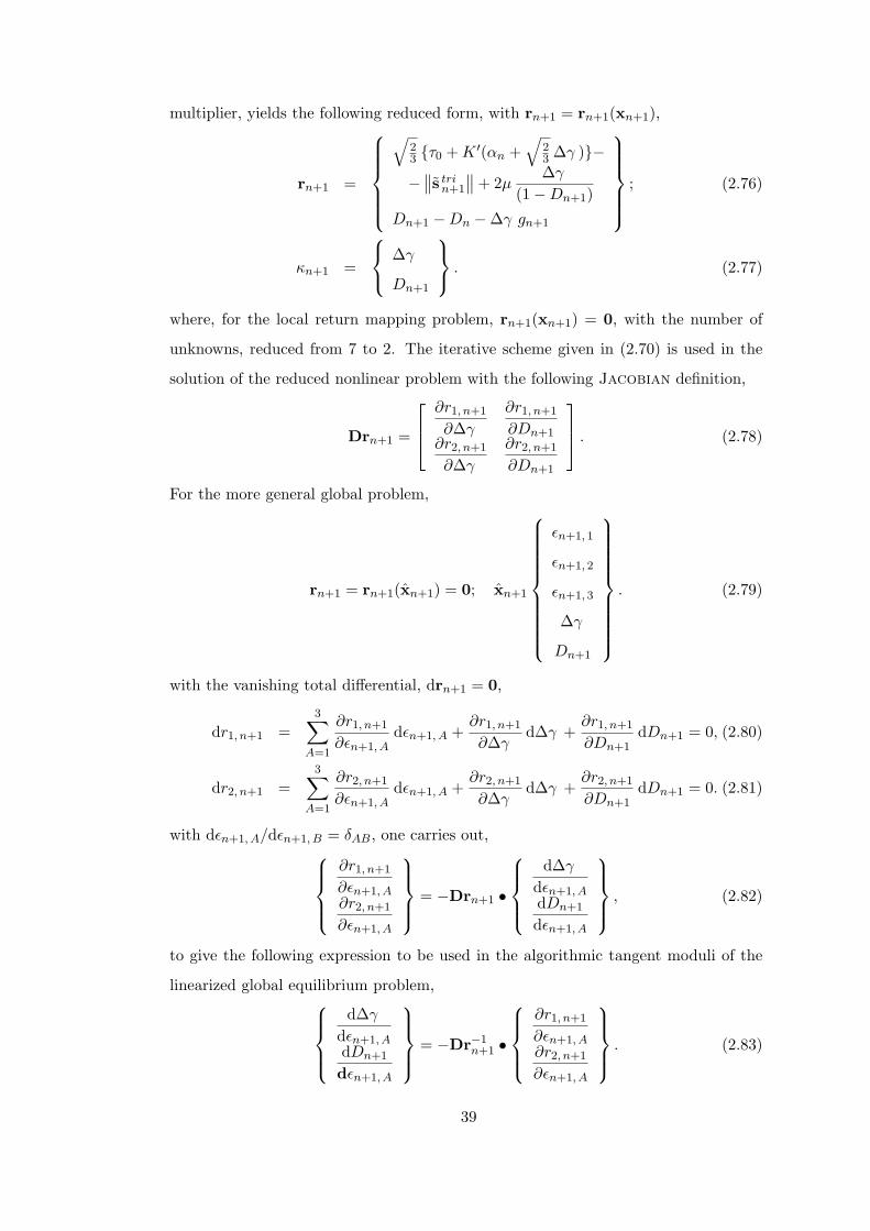
multiplier, yields the following reduced form, with rn+1 = rn+1(xn+1),
rn+1 =
√23 τ0 + K ′(αn +
√23 ∆γ )−
−∥∥s tri
n+1
∥∥+ 2µ∆γ
(1−Dn+1)
Dn+1 −Dn −∆γ gn+1
; (2.76)
κn+1 =
∆γ
Dn+1
. (2.77)
where, for the local return mapping problem, rn+1(xn+1) = 0, with the number of
unknowns, reduced from 7 to 2. The iterative scheme given in (2.70) is used in the
solution of the reduced nonlinear problem with the following Jacobian definition,
Drn+1 =
∂r1, n+1
∂∆γ
∂r1, n+1
∂Dn+1∂r2, n+1
∂∆γ
∂r2, n+1
∂Dn+1
. (2.78)
For the more general global problem,
rn+1 = rn+1(xn+1) = 0; xn+1
εn+1, 1
εn+1, 2
εn+1, 3
∆γ
Dn+1
. (2.79)
with the vanishing total differential, drn+1 = 0,
dr1, n+1 =3∑
A=1
∂r1, n+1
∂εn+1, Adεn+1, A +
∂r1, n+1
∂∆γd∆γ +
∂r1, n+1
∂Dn+1dDn+1 = 0, (2.80)
dr2, n+1 =3∑
A=1
∂r2, n+1
∂εn+1, Adεn+1, A +
∂r2, n+1
∂∆γd∆γ +
∂r2, n+1
∂Dn+1dDn+1 = 0. (2.81)
with dεn+1, A/dεn+1, B = δAB, one carries out,∂r1, n+1
∂εn+1, A∂r2, n+1
∂εn+1, A
= −Drn+1 •
d∆γ
dεn+1, AdDn+1
dεn+1, A
, (2.82)
to give the following expression to be used in the algorithmic tangent moduli of the
linearized global equilibrium problem,d∆γ
dεn+1, AdDn+1
dεn+1, A
= −Dr−1n+1 •
∂r1, n+1
∂εn+1, A∂r2, n+1
∂εn+1, A
. (2.83)
39

Derivations for the components of the local Jacobian, i.e. Drn+1, are listed in
Appendix C, preserving the functional setting. The algorithmic treatment of the
simultaneous approach with reduced two equation system is summarized in Table 2.6.
Table 2.6: Scheme for the return-mapping algorithm for two-step operator-split (Elas-tic predictor-plastic/damage corrector type algorithm).
1. Process Table 2.5. (Elastic predictor),2. Check for plastic-damage loading on effective Kirchhoff stress space,
φtrin+1 = (stri
n+1, 1)2 + (stri
n+1, 2)2 + (stri
n+1, 3)21/2 −
√23τ0 + K(αn)
IF φtrin+1 ≤ 0 THEN
Set (•)n+1 = (•)trin+1, EXIT. (Elastic step)
ELSEGOTO 3. (Plastic-damage corrector)ENDIF3. Find the plastic multiplier and the damage, ∆γ (0) = 0, D
(0)n+1 = Dn, with line-
search,∆γ (k+1)
D(k+1)n+1
=
∆γ (k)
D(k)n+1
− δ(k)
∆(k)n+1
(
∂r2, n+1
∂Dn+1
)(k)
−(
∂r1, n+1
∂Dn+1
)(k)
−(
∂r2, n+1
∂∆γ
)(k) (∂r1, n+1
∂∆γ
)(k)
•
r(k)1, n+1
r(k)2, n+1
with ∆(k)n+1 = det(Dr(k)
n+1) and δ(k) ∈ (0, 1] which denotes the proper line-searchparameter. 4. Return map with the plastic/damage correction,
sn+1, A = s trin+1, A − 2µ
∆γ
(1−Dn+1)s tri
n+1, A∥∥s trin+1
∥∥αn+1 = αn +
√23
∆γ
5. Find the homogenized total Kirchhoff stresses,
τn+1, A = (1−Dn+1) (sn+1, A + pn+1)
6. Update the intermediate configuration,
b en+1, A = J
23 exp
[sn+1, A
µ
], with be
n+1 =3∑
A=1
b en+1, A mtri, A
n+1
40

Reduction to a Single Equation: Following [172], one can further reduce the
number of equations, making use of the condition where, Dn+1 can explicitly be
represented in terms of ∆γ , as follows,
Dn+1(∆γ ) = 1− 2µ∆γ1∥∥s tri
n+1
∥∥−√23 τ0 + K ′(αn +
√23 ∆γ )
. (2.84)
Substituting (2.84) in (2.67), one may carry out a single highly nonlinear equation, in
the residual form,
rn+1 = Dn+1(∆γ )−Dn −∆γ g(Dn+1(∆γ ), Yn+1(∆γ )), (2.85)
where rn+1 = rn+1(κn+1) = 0. The local problem is solved following similar steps as
before, with κn+1 = ∆γ and drn+1 = (∂rn+1/∂∆γ ) dκn+1. For the global problem,
rn+1 = rn+1(xn+1) = 0; xn+1
εn+1, 1
εn+1, 2
εn+1, 3
∆γ
. (2.86)
the vanishing total differential, drn+1 = 0, reads,
drn+1 =3∑
A=1
∂rn+1
∂εn+1, Adεn+1, A +
∂rn+1
∂∆γd∆γ = 0, (2.87)
which gives the following expression, used in the algorithmic material tangent moduli,
d∆γ
dεn+1, A= −(∂rn+1∂∆γ )−1 ∂rn+1
∂εn+1, A, (2.88)
where the derivation of dDn+1/dεn+1, A requires the application of the chain rule of
differentiation, using (2.84), as follows,
dDn+1
dεn+1, A=
∂Dn+1
∂∆γ
∂∆γ
∂εn+1, A, (2.89)
which concludes the simultaneous plasticity-damage solution schemes.
2.3.2.2 Staggered Local Integration Schemes
The plastic/damage corrector phase can be taken in a staggered approach where an
initial plastic correction is done without damage evolution and damage is realized
under frozen plasticity conditions. The result is a three-step, elastic predictor, plastic
41

corrector and damage deteriorator type algorithm, which results in a quite handy
code. This is because simultaneous satisfaction of the whole equation set, given in
(2.68), is not required. The efficiency of such an approach, by bypassing the obligation
of concurrent fulfillment of two nonlinear equations, is also mentioned in [85], in the
context of a two surface damage coupled plasticity model.
To solve the system of equations in a staggered manner, one has to numerically de-
couple the plastic correction and the damage deterioration steps. Below setting shows
the schematic illustration of the problem.
Table 2.7: Three-step operator-split with a staggered plastic/damage correction.
Total Elastic Predictor Plastic Corrector Damage Deteriorator∂tε 6= 0£vbe 6= 0∂tα 6= 0∂tD 6= 0
=
∂tε 6= 0£vbe = 0∂tα = 0∂tD = 0
+
∂tε = 0£vbe 6= 0∂tα 6= 0∂tD = 0
+
∂tε = 0£vbe = 0∂tα = 0∂tD 6= 0
.
Accordingly the plastic correction under frozen damage conditions, i.e. D = Dn,
reads,
rn+1 = rn+1(xn+1)
τn+1, 1 − τ trin+1, 1 + 2µ∆γ nn+1,1
τn+1, 2 − τ trin+1, 2 + 2µ∆γ nn+1,2
τn+1, 3 − τ trin+1, 3 + 2µ∆γ nn+1,3
αn+1 − αn −√
23 ∆γ
qn+1 −K ′(αn+1)
φn+1 := ‖sn+1‖ −√
23 y (qn+1)
; xn+1
τn+1, 1
τn+1, 2
τn+1, 3
∆γ
αn+1
qn+1
.
(2.90)
where rn+1(xn+1) = 0. Following the solution of this set, the damage integration
under constant plastic flow, for the recently found ∆γ , takes place, with the following
modified general mid-point integration,
Dn+1 = Dn + ∆γ [(1− θ) gn + θ gn+θ] , (2.91)
where gn = g(Y d,+n ;αn+1, Dn) with Y d,+
n = Y d,+n (αn+1, Dn), and gn+θ = g(Y d,+
n+θ;
αn+1, Dn+θ) with Y d,+n+θ = Y d,+(αn+1, Dn+θ). In these forms, the requirement of the
42

use of the currently converged equivalent plastic strains, i.e. αn+1, of the plastic cor-
rection step, should be emphasized. (2.91) is merely solved for Dn+1. As a final stage,
damage deterioration is applied to the plastically corrected homogenized principal
stresses, exploiting the effective stress definition as follows,
τn+1, A = (1−Dn+1)τn+1, A
(1−Dn). (2.92)
Reducing the number of equations, the decoupled residuals for plastic correction and
damage integration can be simply written as follows,
rn+1 =
√
23 τ0 + K ′(αn +
√23 ∆γ ) −
∥∥s trin+1
∥∥+ 2µ ∆γ(1−Dn)
Dn+1 −Dn −∆γ [(1− θ) gn + θ gn+θ]
, (2.93)
where rn+1 = 0. With the uncoupled nature of the staggered approach, plasticity
evolves under constant damage and damage evolves under the recently converged
constant plastic multiplier. The linearized version can be given in a compact form as
follows,
dr1, n+1
dr2, n+1
=
∂r1, n+1
∂∆γ
∣∣∣∣D=Dn
0
0∂r2, n+1
∂Dn+1
∣∣∣∣α=αn+1
• d∆γ
dDn+1
. (2.94)
For the global more general problem, using (2.83) together with (2.94) reveals the fol-
lowing explicitly derived forms, which will be used in the algorithmic material tangent
computations,
d∆γ
dεn+1, AdDn+1
dεn+1, A
= −
(∂r1, n+1
∂∆γ
)−1 ∂r1, n+1
∂εn+1, A
∣∣∣∣∣D=Dn(
∂r2, n+1
∂Dn+1
)−1 ∂r2, n+1
∂εn+1, A
∣∣∣∣∣α=αn+1
. (2.95)
The algorithmic treatment of the staggered approach is summarized in Table 2.8. The
efficiency of the use of staggered approach together with an explicit damage integra-
tion, with significantly reduced number of operations, is apparent for the explicit FE
solution procedures, where the process time is controlled mainly by the local integra-
tion computations. Now, the algorithmic moduli derivations for the global solution
schemes, which supplies the quadratic convergence of the iterative procedure once the
sufficiently close initial guess is realized, [166], are visited.
43

Table 2.8: Scheme for the return-mapping algorithm for staggered scheme with three-step operator-split (Elastic predictor-plastic corrector-damage deteriorator type algo-rithm).
1. Process Table 2.5. (Elastic predictor),2. Check for plastic loading on effective Kirchhoff stress space,
φtrin+1 = (stri
n+1, 1)2 + (stri
n+1, 2)2 + (stri
n+1, 3)21/2 −
√23τ0 + K(αn)
IF φtrin+1 ≤ 0 THEN
Set (•)n+1 = (•)trin+1, EXIT. (Elastic step)
ELSEGOTO 3. (Plastic corrector)ENDIF3. Find the plastic multiplier, ∆γ (0) = 0,
∆γ (k+1) = ∆γ (k) − ∂r1, n+1
∂∆γ
∣∣∣∣(k)
D=Dn
r1, n+1|(k)D=Dn
4. Correct plastically the effective Kirchhoff stresses,
sn+1, A = s trin+1, A − 2µ
∆γ
(1−Dn)s tri
n+1, A∥∥s trin+1
∥∥αn+1 = αn +
√23
∆γ
5. Find the current damage, D(0)n+1 = Dn, with line-search,
D(m+1)n+1 = D
(m)n+1 − δ(m) ∂r2, n+1
∂Dn+1
∣∣∣∣(m)
α=αn+1
r2, n+1|(m)α=αn+1
with δ(m) ∈ (0, 1], which denotes the proper line-search parameter.6. Apply the damage deterioration,
τn+1, A = (1−Dn+1) (sn+1, A + pn+1)
7. Update the intermediate configuration,
b en+1, A = J
23 exp
[sn+1, A
µ
], with be
n+1 =3∑
A=1
b en+1, A mtri, A
n+1 .
2.3.3 Consistent Tangent Moduli
In the global more general problem, τ = τ (ε,∆γ (ε), D(ε)), where the spectral decom-
position of the homogenized Kirchhoff stress tensor, i.e. τn+1 = (1 −Dn+1) τn+1,
44

for t = tn+1 is,
τn+1 =3∑
A=1
τn+1, A mtri, An+1 . (2.96)
Following relation gives the definition of the spatial elasto-plastic-damage tangent
moduli, [161],
cijkl = 2FiI FjJ FkK FlL∂SIJ
∂CKL, (2.97)
which is a push-forward transformation of material tangent. S = F−1 • τ • F−T ,
is the Second Piola Kirchhoff stress tensor, i.e. the pull-back transform of the
Kirchhoff stress tensor and C is the right Cauchy-Green deformation tensor. An
explicit representation of the tensor can be given as,
C =3∑
A=1
3∑B=1
aepdn+1, AB mtri, A
n+1 ⊗mtri, Bn+1 + 2
3∑A=1
τn+1, ACtri,An+1 . (2.98)
Starting with the first part of (3.84), aepdn+1, AB is the following 3× 3 matrix 8,
aepdn+1, AB =
dτn+1, A
dεtrin+1, B
, (2.99)
the computation of which requires the following chain rule of differentiation,
dτn+1, A
dεtrin+1, B
=∂τn+1, A
∂εtrin+1, B
+∂τn+1, A
∂∆γ
∂∆γ
∂εtrin+1, B
+∂τn+1, A
∂Dn+1
∂Dn+1
∂εtrin+1, B
, (2.100)
with
∂τn+1, A
∂εtrin+1, B
= (1−Dn+1)∂τ tri
n+1, A
∂εtrin+1, B
− 2µ∆γ∂nn+1, A
∂εtrin+1, B
(2.101)
∂τn+1, A
∂∆γ= −2µnn+1, A (2.102)
∂τn+1, A
∂Dn+1= −τ tri
n+1, A. (2.103)
Using δdevAB = δAB− 1
3 , with δAB representing the Kronecker delta which is given as,
δAB =
1, if A = B;
0, otherwise.(2.104)
one can find,
∂τ trin+1, A
∂εtrin+1, B
= H + 2µδdevAB, (2.105)
∂nn+1, A
∂εtrin+1, B
=2µ∥∥s trin+1
∥∥ δdevAB − nn+1, A nn+1, B. (2.106)
8 Taking the differential of the trial logarithmic elastic strains, i.e. ε e, trin+1 = ε n+1− ε p
n, will result
in, dε e, trin+1 = dε n+1 − dε p
n. Since for t = tn+1, dε pn = 0, dε e, tri
n+1 = dε n+1.
45

In § 2.3.2.1 and § 2.3.2.2, the expressions, ∂∆γ /∂εn+1 and ∂Dn+1/∂εn+1 in principal
components, are already supplied for different integration schemes. Exploiting the
previously derived dε e, trin+1 = dεn+1, the outcomes for ∂∆γ /∂ε e, tri
n+1 and ∂Dn+1/∂ε e, trin+1
can be found. Accordingly, making use of (2.83) for the simultaneous scheme with two
equations, (2.88) and (2.89) for the simultaneous scheme with a single equation, and
finally (2.95) for the staggered approach with two equations, with the substitution
∂εn+1 → ∂ε e, trin+1 , is sufficient. Unreduced sets involve rather lengthy derivations,
which are not included here.
It is noteworthy that, in case of no damage coupling, aepdn+1 boils down to aep
n+1 given in
[161], for nonlinear isotropic hardening finite plasticity formulated in principal axes.
Coming to the second part of (3.84), Ctri,An+1 is the spectral direction variation in the
form of eigen-dyad derivatives with respect to the Eulerian metric tensor (rota-
tion of the eigen-bases). The derivation reveals the following expression with eigen-
projections9, see, e.g. [167] and [161].
Ctri,An+1 =
1DA
[Ibe, trin+1 − b e, tri
n+1 ⊗ b e, trin+1 + I3 λe, tri,−2
n+1, A (1⊗ 1− I)]
+1
DA[λe, tri, 2
n+1, A (b e, trin+1 ⊗mtri, A
n+1 + mtri, An+1 ⊗ b e, tri
n+1 )
− 12D′
A λe, trin+1, Amtri, A
n+1 ⊗mtri, An+1 ]
− 1DA
[I3 λe, tri,−2n+1, A (1⊗mtri, A
n+1 + mtri, An+1 ⊗ 1)],
(2.107)
where,
I =12(1⊕ 1 + 1 1), (2.108)
Ibe, trin+1 =
12(be, tri
n+1 ⊕ be, trin+1 + be, tri
n+1 be, trin+1 ), (2.109)
and,
D′A = 8λe, tri, 3
n+1, A − 2I1λe, trin+1, A − 2I3λ
e, tri,−3n+1, A . (2.110)
(2.73) and (2.107) require computation of DA, which is given in (2.53). An explicit
designation of DA may be furnished as, DA = (λe, tri, 2n+1, A − λe, tri, 2
n+1, B) (λe, tri, 2n+1, A − λe, tri, 2
n+1, C),
where an even permutation of indices (1, 2, 3) is denoted by (A,B, C), [167]. (2.73)
and (2.107), suffer from singularities or ill-conditioning, for equal or nearly equal
9 The fourth order tensor can also be computed using eigenvectors. [121] shows that an use ofeigen-bases ends up with a faster computation.
46

eigenvalues, respectively, with DA → 0. In treatment of such cases, different methods,
analytical or numerical, are suggested. As an analytical approach, [130, pp. 338–
341], in the context of eigen-vector formulation, uses systematic application of the
L’Hospital rule to create special expressions for diverse situations. Coming to the
numerical methods, the use of perturbation schemes are common, where equal or
numerically close eigenvalues are perturbed to have distinct values. This enables
treatment of these special cases in the general class of distinct eigenvalues, making
use of (2.73) and (2.107). In the current study, due to its feasibility, this latter
approach is used. Accordingly for sufficiently close λe, trin+1, A and λe, tri
n+1, B, the following
perturbation scheme is applied, [119],λe, tri
n+1, A
λe, trin+1, B
λe, trin+1, C
=
(1 + δ) λe, tri
n+1, A
(1− δ) λe, trin+1, B
1/[(1 + δ)(1− δ)]λe, trin+1, C
, with δ 1. (2.111)
2.3.4 Expansion to Kinematic Hardening
For the sake of completeness, the algorithmic forms for the simultaneous scheme are
involved for combined isotropic kinematic hardening plasticity coupled with damage.
Accordingly, the definition of the trial state additionally requires,
z trin+1 = zn. (2.112)
The spectral decomposition of z trin+1, A read, z tri
n+1, A = γ tri, 2n+1, A = γ 2
n, A, for both Model
A and Model B,
z trin+1 =
3∑A=1
γ tri, 2n+1, A νtri, A
n+1 ⊗ νtri, An+1 , (2.113)
where the algorithmic counterpart of the evolution equation of the kinematic hardening
strain like variable is,
£vzn+1 = −2 γn+1 ∂βφ∣∣∣n+1
• zn+1; Model A;4z n+1 = −γn+1 ∂βφ
∣∣∣n+1
; Model B.(2.114)
Utilizing exponential mapping and backward Euler method for integration of Model
A and Model B, respectively, one has,
zn+1 = exp[2 ∆γ ∂βφ
∣∣∣n+1
]• z tri
n+1; Model A;
zn+1 = z trin+1 + ∆γ ∂βφ
∣∣∣n+1
; Model B.(2.115)
47

Refining (2.115) to constitute the principal stretches, one carries out,
γn+1, A = exp[∆γ ∂φ
∂βA
∣∣∣n+1
]γ tri
n+1, A; Model A;
γn+1, A = γ trin+1, A + ∆γ ∂φ
∂βA
∣∣∣n+1
; Model B.(2.116)
For Model A, taking the natural logarithms of both sides, one obtains the following
relation,
κn+1, A = κ trin+1, A + ∆γ
∂φ
∂βA
∣∣∣∣∣n+1
, (2.117)
Eventually one has,
κn+1, A = κ trin+1, A −∆κn+1, A; Model A;
zn+1, A = z trin+1, A −∆z p
n+1, A; Model B.(2.118)
where the principal strain corrections read,
∆κn+1, A = ∆γ ∂φ∂βA
∣∣∣n+1
; Model A;
∆zn+1, A = ∆γ ∂φ∂βA
∣∣∣n+1
; Model B.(2.119)
In the current setting, since the back stress and the stress tensors commute, the
exponential mapping is exactly satisfied, [57], and the use of the principal components
rather than tensorial descriptions become available. Unless the coaxiality is presumed,
the reduction of the forms to the principal space is not possible.
It is noteworthy that since the stress corrections in the deviatoric Kirchhoff stress
space for the back stress give identical results for Model A and Model B, such as,
βn+1, A = β trin+1, A +
23C ∆γ nn+1, A. (2.120)
Final equation to be satisfied is the yield function computed at the current step,
φn+1 := ‖ξ n+1‖ −√
23
y (qn+1) = 0. (2.121)
In a residual setting, using the effective stresses definition with (2.63), for the current
and the trial principal stress components, the complete simultaneous set of equations
48

can be given as,
rn+1 =
τn+1, A − τ trin+1, A + 2µ∆γ nn+1, A
βn+1, A − β trin+1, A − (2/3)C(θ) ∆γ nn+1, A
αn+1 − αn −√
23 ∆γ
qn+1 −K ′ (αn+1)
φn+1 := ‖ξ n+1‖ −√
23 y (qn+1)
Dn+1 −Dn −∆γ gn+1
; xn+1
τn+1, A
βn+1, A
∆γ
Dn+1
αn+1
qn+1
.
(2.122)
with (A = 1, 2, 3). where rn+1(xn+1) = 0. Following [166], the local governing equa-
tions collected in (2.122) can be reduced, particularly for the chosen yield criterion,
making use of the substitution, ξn+1, A = ‖ξ n+1‖ nn+1, A
sn+1−βn+1 = s trin+1−β tri
n+1 −
2µ∆γ
(1−Dn+1)+
23C ∆γ
nn+1, (2.123)
‖ξ n+1‖ nn+1, A =∥∥ξ tri
n+1
∥∥ n trin+1, A (2.124)
−
2µ∆γ
(1−Dn+1)+
23C ∆γ
nn+1, A.
Applying the following arrangements,(‖ξ n+1‖+ 2µ
∆γ
(1−Dn+1)+
23C ∆γ
)nn+1, A =
∥∥ξ trin+1
∥∥ n trin+1, A, (2.125)
and exploiting the condition of collinear flow and the trial Kirchhoff stress tensor,
where, nn+1 ≡ n trin+1, [166], the uniqueness of the spectral decomposition yields,
n trin+1, A mtri, A
n+1 = nn+1, A mAn+1, (2.126)
which gives mtri, An+1 ≡ mA
n+1 and nn+1, A ≡ n trin+1, A. Utilizing this equivalence, one can
write,
‖ξ n+1‖+ 2µ∆γ
(1−Dn+1)+
23C ∆γ =
∥∥ξ trin+1
∥∥ . (2.127)
Finally, representing the hardening/softening function definition in terms of the plastic
multiplier, yields the following reduced form,
rn+1 = rn+1(xn+1) =
√23 τ0 + K ′(αn +
√23 ∆γ )
−∥∥ξ tri
n+1
∥∥+ 2µ∆γ
(1−Dn+1)+
23C ∆γ
Dn+1 −Dn −∆γ gn+1
;(2.128)
xn+1 =
∆γ
Dn+1
. (2.129)
49

where, for the local return mapping problem follows identical steps with the previously
proposed simultaneous routines.
2.4 Application Problems
The given framework is implemented as a user defined material subroutines, UMAT for
ABAQUS/Standard, VUMAT for ABAQUS/Explicit and UFINITE10, for MSC.Marc,
for return mapping in the company of reduced equation couple, together with the
simultaneous and the staggered solution schemes which are listed in Table 2.6 and
Table 2.8. The staggered solution schemes are supplied with forward (explicit) and
backward (implicit) Euler integration for the D. The codes are materialized in
accuracy and efficiency assessment of the integration routines and in the simulation of
a set of axi-symmetric application problems. Throughout the simulations, a saturation
type isotropic hardening function is utilized for plasticity, which is given as,
K ′ (α) = K α + (K∞ −K0) (1− exp [−δ α]) .
For damage evolution, following simplified Lemaitre model is selected,
g(Y ;α, D) =a
(1−D)Y,
with Y = Y d, +.
2.4.1 Geometrical Interpretation and Accuracy and Efficiency Assess-
ment of the Return Map Algorithms
In this first set of application problems, the geometrical insight into the simultaneous
and staggered return mapping algorithms is presented. Moreover accuracy and effi-
ciency assessment studies are given which shows relative reliability and performance
of the methods for a given strain increment.
10 UFINITE serves a suitable environment for isotropic finite strain elasto-plasticity defined byprincipal stretches. Implementation details of UFINITE are well documented in [125, Chp. 3, pp.280–282].
50

2.4.1.1 Geometrical Interpretation
Damage softening and isotropic plastic hardening are in competition for a damage
coupled plasticity. A geometrical insight into the problem may be supplied by pre-
senting the iterative return map for a given trial stress state on the Π plane. For this
purpose, following hypothetical material properties given in Table 2.9, which gives
geometrically clear resultants, are selected. Besides, an initial 1D stress state on the
yield surface is selected, free of any initial plastic strains or damage.
Table 2.9: Material parameters for the example problem.
Parameter Symbol Magnitude UnitBulk modulus H 175 GPaShear modulus µ 80.7692 GPaFlow stress τ0 0.750 GPaSaturation stress τ∞ 5 GPaLinear hardening K 0.1 GPaHardening exponent δ 10 -Damage multiplier a 30 -
Resultant return mapping patterns for a set of strain increments on the Π plane are
given for the simultaneous integration algorithm in Figure 2.4. It is seen that an
arbitrary elastic trial state is followed by a single plastic/damage correction step. The
first observation is the radial character of the return map, where any trial stress state
is mapped with a direction normal to the circular yield locus. A noteworthy fact is
that, the yield locus on the effective stress space is expanding with plastic hardening
whereas damage effect results in a shrinkage on the yield locus represented at the
homogenized stress space.
Once the same problem is repeated for the staggered routine, the pattern given in
Figure 2.5 is carried out. This time, the radial return requires two additional steps,
51

Figure 2.4: Geometrical representation of the return map for the simultaneous inte-gration scheme.
named as plastic correction and damage deterioration, for an arbitrary elastic trial
state. Other observations follows the previous solution’s results where the difference
in between Figure 2.4 and Figure 2.5 is hardly observed which shows the performance
of a staggered routine which assumes uncoupled plasticity and damage.
Figure 2.5: Geometrical representation of the return map for the staggered integrationscheme.
52

2.4.1.2 Accuracy Assessment - Isoerror Maps
Isoerror maps lack mathematical rigor however they are very effective in evaluation of
the accuracy of the integration routines. The effect of damage integration approaches,
such as simultaneous or staggered implicit/explicit, damage functional degree of non-
linearity and initial damage on the effect of integration accuracies, is investigated.
The material parameters utilized are in variance with those of the previous case where
τ∞=1 GPa and a=1.5 are utilized.
Use of isoerror maps goes back to [93]. An example use may be seen in [131] among
others. In damage mechanics, use of isoerror maps is seen in [194]. In the current
context, the method is applied for a 3D case. Test point locations are shown Figure
2.6 for the effective Kirchhoff stress space where totally four conditions, namely
I-A, I-B, II-A and II-B, are analyzed.
Figure 2.6: Representation of the test points on the Π plane.
I stands for the stress states for no initial pressure and II stands for the pressurized
initial state, as seen in selected planes in Haigh-Westergaard space in Figure
2.6.a. Pressurized cases are to investigate the effect of initial pressure on damage
evolution. Figure 2.6.b represents the yield locus on the Π plane, where the marked
53

point A stands for the uniaxial stress state whereas point B stands for the state with
pure shear condition. Deviatoric loads, on the Π plane, tangential and normal to
the circular yield locus, as shown in Figure 2.6.b, are applied for the test points and
regarding isoerror maps are plotted. Any point on the Π plane on the yield locus can
be uniquely defined for a given pressure, Lode angle and yield stress. Depending on
the x and y coordinates of the point on the yield locus, the initial principal stress state
definition given in (2.130) can be derived for a given pressure, p, and yield stress, τ0,
[76, p. 18],
τ p = W • v, (2.130)
where following definitions are valid
τ p =
τ1
τ2
τ3
, W =
−1/2 −1/6 1
1/2 −1/6 1
0 1/3 1
, (2.131)
together with the specialized v values, vA and vB, for points A and B, respectively,
which are given as,
vA =
0
2τ0
p
, vB =
2τ0/
√3
0
p
. (2.132)
Accordingly, for points I-A, I-B, II-A, II-B, the initial stress and strain states are
quantitatively given in Table 2.10, for τ0 = 750 MPa,
Table 2.10: Initial conditions of the selected points.
Test Point τ =
τ1, τ2, τ3
tεe=
εe1, εe
2, εe3
t
I-A
−250−250
500
−1.547619047619048e-003−1.547619047619048e-003
3.095238095238095e-003
I-B
−4.330127018922194e+002
4.330127018922194e+0020
−2.680554821237549e-0032.680554821237549e-003
0
II-A
00
750
−1.071428571428571e-0031.071428571428571e-0033.571428571428571e-003
II-B
−1.830127018922193e+002
6.830127018922194e+0022.500000000000000e+002
−2.204364345047072e-0033.156745297428025e-0034.761904761904762e-004
54

As seen for cases of I no initial pressure is due and for II initial pressure with τ0/3 is
assigned. Since the loads applied lie on the deviatoric Π plane, they also are deviatoric.
In numerical accuracy assessment of the integration algorithms, true percent relative
errors are computed for different fields. For the stress field, the definition of the error
in stress, ERRτ , follows as,
ERRτ =
√[τexact − τapproximate] : [τexact − τapproximate]√
τexact : τexact× 100. (2.133)
Error is also computed for D and α, which is the radial location of the point on the
circular yield surface. For these scalar fields, error formulation utilizes the conventional
form. Accordingly for [F] representing any one of D or α, the error ERRF becomes,
ERRF =|Fexact−Fapproximate|
|Fexact|× 100. (2.134)
In above computations approximate values are computed with a single step application
of the algorithm for the given loading whereas the exact values utilizes 1000 steps,
following the common approach in the literature. A 5 percent error can be taken as
an acceptable threshold in evaluation of the results. Resultant isoerror maps are given
in Figures 2.7, 2.8, 2.9 and 2.10 for test points I-A, II-A, I-B and II-B, respectively.
In the representations, columns 1 to 3, respectively designate the isoerror plots for
effective stress, equivalent plastic strain and damage errors. Coming to the rows,
simultaneous, staggered implicit and staggered explicit schemes are respectively given
in row a, b and c.
The difference in the results for difference test points is hardly recognizable. Among
the results for integration routines, it is seen that for small strain increments the differ-
ence is not obvious however for large strain increments the difference gets importance.
Thus one should utilize staggered explicit routines only for small strain increments.
In this setting, increasing the number of steps to gain accuracy may increase the com-
putational time thus tempting staggered routine may not be so efficient. However, the
result is problem specific. It is shown that once the coupling in between damage and
plasticity is omitted, the implicit integration of damage can only increase the damage
integration quality to a certain level especially for large loading steps.
55

Figure 2.7: Isoerror maps for accuracy assessment of integration algorithms for caseI-A.
56

Figure 2.8: Isoerror maps for accuracy assessment of integration algorithms for caseII-A.
57

Figure 2.9: Isoerror maps for accuracy assessment of integration algorithms for caseI-B.
58

Figure 2.10: Isoerror maps for accuracy assessment of integration algorithms for caseII-B.
59

2.4.1.3 Efficiency Assessment - Convergence Tests
In this section, the concentration is devoted to the number of iterations required in
different solution algorithms for a given initial condition and applied load step. For a
point lying on the yield locus a logarithmic strain based loading with a magnitude of
0.015 in radial and tangential directions are applied, which for an exact solution cre-
ates, a final equivalent plastic strain of 0.018925584826 and damage of 0.033566948053.
In the solutions, a convergence threshold of 10e-6 is utilized.
Table 2.11 lists of the equivalent plastic strain and damage values at each iteration
for the simultaneous scheme with two reduced equations. As seen, desired precision
is satisfied at the sixth iteration.
Table 2.11: Convergence of equivalent plastic strain and damage through iterations,simultaneous scheme.
Iteration α D
1 4.706284481469381E-003 0.6213810306702642 1.459249815639381E-002 2.202923716197214E-0023 1.863027071136262E-002 8.214544668329469E-0034 1.819276851166353E-002 3.457503808154121E-0025 1.819101038280528E-002 3.458794550210217E-0026 1.819101021947922E-002 3.458795530809459E-002
The residuals of the reduced equations are given in Table 2.12 from which the quadratic
convergence quality of the local integration scheme is observed.
Table 2.12: Convergence of the residuals through iterations, simultaneous scheme.
Iteration r1 r2
1 -1674.96750537952 0.3344838008748142 -1015.13544326820 -0.1570435474480213 -14.1780168970472 -2.787756928654985E-0024 0.406715354483822 2.728864735388609E-0055 -5.422106369223911E-006 -1.037531647402057E-0086 -9.094947017729282E-013 -1.387778780781446E-017
60

For the same problem, once a staggered routine is utilized, plastic integration is fol-
lowed by damage integration. Accordingly, the plastic correction, which is identical for
implicit and explicit damage integration, results in the convergence behavior, which
requires only three iterations for convergence, due to the character of hardening plas-
ticity models, as given in Table 2.13.
Table 2.13: Convergence of the equivalent plastic strain and residual through itera-tions, plastic correction phase of the staggered scheme.
Iteration α r1
1 1.882513792587752E-002 -3.400262476735412 1.883826792142717E-002 -1.457530743209645E-0063 1.883826792705538E-002 0.000000000000000E+000
With an implicit damage integration, convergence is captured in three iterations as
given in Table 2.14.
Table 2.14: Convergence of the damage and residual through iterations, damage de-terioration phase of the staggered scheme.
Iteration D r2
1 2.339278937801977E-002 -5.682196415299837E-0042 2.378950956521546E-002 -1.997380615348376E-0073 2.378964911673556E-002 -2.477532068390076E-014
For explicit damage integration, obviously the first line of the implicit damage inte-
gration may be taken, which stands for a forward damage integration. The results
show that, maximum error in damage is observed in the explicit damage integration
together with the staggered routine. Since number of iterations is a direct measure
of number of floating point calculations, it has an indispensable effect on the overall
computational time required thus the efficiency. However, although total number of
iterations seems identical in simultaneous and staggered routine with implicit damage
integration, number of floating point operations of the simultaneous routine is larger
due to the requirement for additional computations of the off diagonal members of the
61

Jacobian. It should be noted that, although their implementation is much easier, as
the coupled terms of the Jacobian are not computed, there is a trade off between
accuracy and efficiency for staggered routines. Thus, the selection of whether a fully
coupled or uncoupled solution scheme depends on the problem nature which is related
to the degree of nonlinearity of the damage function, and degree of coupling between
plasticity and damage. As the results represent, for favorable conditions staggered
routines with explicit integration may be quite efficient. This property is valid espe-
cially for dynamic explicit problems where the time steps in global solution may be
quite small which satisfies the conditional stability of the global problem.
2.4.2 Necking of an Axi-symmetric Bar
This example is well documented in the literature, see, e.g. [181], [161]. The problem
illustrates the necking of an axi-symmetric bar with a total length of 53.334 and radius
of 6.413. In order to trigger necking a total 98.2% radial reduction is introduced to the
center, which is linearly distributed throughout the length of the bar. This way, the
bifurcation problem, where the necking can emanate at any section, is transferred into
a limit load problem, [80]. The geometry of the modeled quarter, 20x10 FE mesh (20
elements on longitudinal direction, 10 elements on radial direction) and the boundary
conditions can be seen in Figure 2.11. It should be noted that, this problem does not
reflect the active-passive conditions of damage evolution, as it is mainly an overall
tensile processes.
The problem is solved for damage coupled and no damage (plain von Mises plastic-
ity) cases where damage coupled simulations are conducted using simultaneous and
staggered solution schemes with two local equations, presented in the previous sec-
tions. For the staggered schemes, explicit and implicit damage integration procedures
are followed. In the simulations, 250 load steps are applied for a total top displace-
ment of ∆u=7.68. Premature failure (termination before increment 250) is observed
in damage coupled models, whereas for the no damage case all load increments are
successfully applied.
62

Figure 2.11: 20x10 mesh, boundary conditions and the geometry for the simulation ofnecking of an axi-symmetric bar.
A large strain, updated Lagrange formulation is selected where multiplicative de-
composition is set as a plasticity procedure. Mechanical Element 10, with a selective
integration scheme is used for axi-symmetric analyses 11.
The material parameters, fully compatible with [181], are given in Table 2.15. Unless
otherwise stated, these parameters apply for all the other example problems.
Table 2.15: Material parameters for the example problem.
Parameter Symbol Magnitude UnitBulk modulus H 164.206 GPaShear modulus µ 80.1938 GPaFlow stress τ0 0.450 GPaSaturation stress τ∞ 0.715 GPaLinear hardening K 0.12914 GPaHardening exponent δ 16.93 -Damage multiplier a 200 -
11 It should be noted that the derivations of this chapter are made within the context of standardFE formulations. The plastic incompressibility acts as an over-constraint on the pressure field whichresults in locking of the standard finite elements. MSC.Marc, utilizes a mixed formulation, to bemore specific a two-field, perturbed Lagrangian form of a variational principle, for treatment ofquasi-incompressibility, in the multiplicative framework. The formulations are well documented in[124, Chp. 5, pp. 158–162]. Since proposing a variational structure is beyond the scope of this thesis,we are contented with a suitable application of the exactly derived forms to the given framework inthe space of approximation errors.
63

Damage and equivalent plastic strain distributions, just before the fracture, at ∆u=4.9152,
computed with the simultaneous scheme, are given in Figure 2.12. At the mid zone
of the bar, due to the localized deformation together with necking, equivalent plastic
strains and damage shows a marked accumulation. Moreover, it is observed that the
distribution of highly localized damage has a central character which causes the local
failure. This finding is in correlation with the actual experimental facts, where cen-
ter constitutes the zone of ductile failure initiation (cup-cone fracture). Unlike [181],
where a deviatoric variant of Lemaitre damage model is utilized, the patterns of
damage and equivalent plastic strains show a certain deviation. This is due to domi-
nating effect of the triaxiality in the current model. For metal plasticity, disregarding
the volumetric response is not realistic on physical grounds.
Figure 2.12: Contour plots for the damage coupled model at ∆u=4.9152 (simultane-ous two equation solution scheme), (top) Damage distribution, (bottom) Equivalentplastic strain distribution.
The load-displacement curves in Figure 2.13 show that, introduction of damage cou-
pling results in a steeper post peak response with a premature termination of the anal-
ysis at smaller strains. This anticipated result with a considerable loss in ductility, is
due to the strength loss of the material with damage deterioration. The same figure
also shows that, the resultant responses for the simulated local integration schemes,
64

such as simultaneous, staggered with explicit damage integration and staggered with
implicit damage integration, do not deviate from each other. This is primarily due to
the selected functional forms for plasticity and damage and used material parameters,
which govern the mathematical character of the problem at the space of unknowns,
in terms of the degrees of functional nonlinearities. Besides, utilized sufficiently large
number of loading steps has a stabilizing effect by improving the accuracy of the ex-
plicit damage integration steps. Use of implicit plastic integration as a first step for
both of the staggered cases helps as well. The excessive number of tests conducted by
the researchers show that, simultaneous scheme and the damage implicit integration
in the staggered scheme should be supplied with appropriately defined line-searches
and backtracking. For this purpose, Table 2.6 and Table 2.8 use particular Newton
iteration steps, scaled with a line-search parameter, regarding these cases.
Figure 2.13: Load-displacement curves for damage coupled and non-damaged plastic-ity models.
65

2.4.3 Axi-symmetric Tension of a Notched Specimen
This example includes a notched specimen under tensile loading. The notch creates a
radius dependent nonuniform stress state, which affects the damage deriving mecha-
nisms. The geometry is the one utilized in [37] and [187]. Dimensions, the FE mesh
and the imposed boundary conditions are given in Figure 2.14. In the simulations 250
load steps are applied for a total top displacement of ∆u=1.00. Just like the previous
one, this problem is also solved for damage coupled (with simultaneous and staggered
schemes) and no damage cases. Due to its overall tensile character, this problem also
does not reflect the effect of quasi-unilateral damage evolution.
Figure 2.14: Mesh, boundary conditions and the geometry for the simulation of axi-symmetric tension of a notched specimen.
The results follow a similar fashion with the ones recorded in the literature as far
as the damage evolution throughout the tensile process is taken into account. An
initially notch concentrated damage, tends to slowly move towards the center and
localize. This triaxiality dependent trend throughout the deformation history, given
in Figure 2.15, is in complete accordance with the experimental evidences showing
central failure initiation for certain notch geometries, [74].
The load-displacement curves in Figure 2.16 (left) show that, deteriorative mecha-
nism of damage results in a softer response for damage coupled models compared to
no damage case. The deviation between damage coupled and no damage cases’ curves
66

Figure 2.15: Contour plots of the Damage distribution at different steps (simulta-neous two equation solution scheme), (top row, from left to right) ∆u=0.032, 0.052and 0.104, (bottom row, from left to right) ∆u=0.440, 0.800 and 0.916.
increase with increasing damage accumulation controlled by the plastic deformation.
The response curves for the utilized local integration schemes are in complete corre-
lation within each other with the identical reasons listed for the previous example.
Figure 2.16 (right) shows the damage histories computed at the notch center with dif-
ferent integration schemes, which also are in perfect harmony. The curves get steeper,
with a concave up structure, towards the local failure point, where damage reaches
the limit value, i.e. D = 1. This marked increase in damage increments near failure
creates numerical difficulties in implicit schemes, [187], where the use of line-search
becomes indispensable.
67

Figure 2.16: History plots, (left) Load-displacement curves for damage coupled andnon-damaged plasticity models, (right) Damage evolution at center for various localintegration schemes.
2.4.4 Upsetting of an Axi-symmetric Billet
Final problem is concerned with the upsetting of an axi-symmetric billet, which aims
to investigate the effect of crack closure effect on the resultant damage distributions.
For this purpose, on a cylindrical billet with a total undeformed length of 30.0 and
radius of 10.0, two simulations are realized one of which involves the crack closure
effect with the crack closure parameter, h = 0.01, and the other does not give account
for the quasi-unilateral damage evolution. The geometry, mesh and imposed boundary
conditions are given in Figure 2.17. At the die-billet interface, tangential movement
is completely restrained using the glue contact option. A similar problem is studied
for isotropic porous plasticity in [174]. The material parameters are the ones listed in
Table 2.15, with a slight difference with a = 2.0. In determination of the results, the
simultaneous local integration scheme with two equations, is utilized.
The upsetting is realized for over 60% height reduction. With the applied friction
conditions, which provides a perfect stick at the die-billet interface, barreling occurs.
Figure 2.18 (left) shows the deformed FE mesh at ∆u=9.126. The equivalent plastic
68

Figure 2.17: Mesh, boundary conditions and the geometry for the simulation of up-setting of an axi-symmetric billet.
strain contours plotted for two simulations, with and without crack closure effect,
show a complete accordance as seen in Figure 2.18 (right) and (middle) respectively.
With J2 theory, the plastic flow and the accumulated equivalent plastic strains, which
stands for the numerical construct for the micro-mechanical dislocation pile-ups, are
functions of the distortional elastic energies. In the damage coupled framework, the
plasticity is assumed to perform on the effective material subscale. Mathematically,
this is realized by the damage free effective stress space formulation of plasticity, where
for low levels of damage, the effective isochoric energies do not deviate considerably,
which reveals the correlation of these plots.
A marked difference, in terms of intensity and distribution, is observed in the final
damage contours between two simulations as seen in Figure 2.19. The reason for the
difference in intensities, where the damage model without quasi-unilateral conditions
has a peak damage value of more than 15 times of the model with crack closure
effect for ∆u=9.126, is apparent. Without incorporation of the crack closure effect,
the intensity of damage increments utilize complete elastic energy release without
making distinction about the governing stress terms’ compressive or tensile characters,
which results in a higher rate of accumulation. With crack closure effect however,
69

Figure 2.18: Resultants at ∆u=9.126 (simultaneous two equation solution scheme),(left) Deformed mesh, (middle) Equivalent plastic strain distribution without crackclosure effect, (right) Equivalent plastic strain distribution with crack closure effect,h = 0:01.
Figure 2.19: Contour plots of the Damage distribution at ∆u=9.126 (simultaneoustwo equation solution scheme), (left) without crack closure effect, (right) with crackclosure effect, h = 0:01.
although the involvement of the energy release due to tensile principal stresses is
complete, for compressive principal stresses it is only partial, where the extent of its
contribution is scaled by the selected crack closure parameter. On the deviation in
70

distributions, following comments can be made. As Figures 2.18 and 2.19 reveal, the
damage distribution primarily follows a pattern similar to the ones of the equivalent
plastic strains, in the absence of the crack closure effect. This anticipated result is
due to the strong-coupled plasticity-damage framework.
Figure 2.20, which shows the stress state, at ∆u=9.126, in terms of three principal
components of Cauchy type, is helpful in evaluation of the case with crack closure
effect. Comparison of the zones of the positive principal stresses, which are purposely
highlighted in Figure 2.20, and the damage accumulations given in Figure 2.19 (right),
one may conclude that, in the advancing steps of frictional upsetting, together with
barreling, the tensile pressures at the equator line has a dominating role on the dam-
age evolution if the crack closure effect is incorporated. Occurrence of surface cracks
due to barreling in frictional upsetting processes is a known experimental fact. Conse-
quently, recalling previously mentioned ductile damage micro-mechanism, formed of
micro-voids nucleation, growth and coalescence, use of quasi-unilateral evolutionary
conditions is motivated. Accordingly, in engineering practice, utilizing a combined
experimental-numerical procedure, in the definition of an appropriate crack closure
parameter is vital. Utilizing this fact, one may also make a final remark on the ob-
vious role of friction on the eventual damage distributions, [174]. For the frictionless
upsetting where a homogeneous deformation is due, a quasi-unilaterally evolving dam-
age model with the current utilization predicts a homogeneous damage accumulation,
which is merely due to partially contributed uniform compressive stresses, where the
extent of this contribution depends solely on the selected crack closure parameter.
2.5 Conclusion
In this chapter, a local, damage coupled isotropic finite strain hyperelastic-plastic
framework is formulated in the principal axes, in a Euclidean setting. The unified
functional framework for the governing functions of isotropic hardening plasticity and
damage does not assume particular restrictions on the forms. This gives rise to im-
plementation of a broad range of isotropic hardening plasticity and damage models,
71
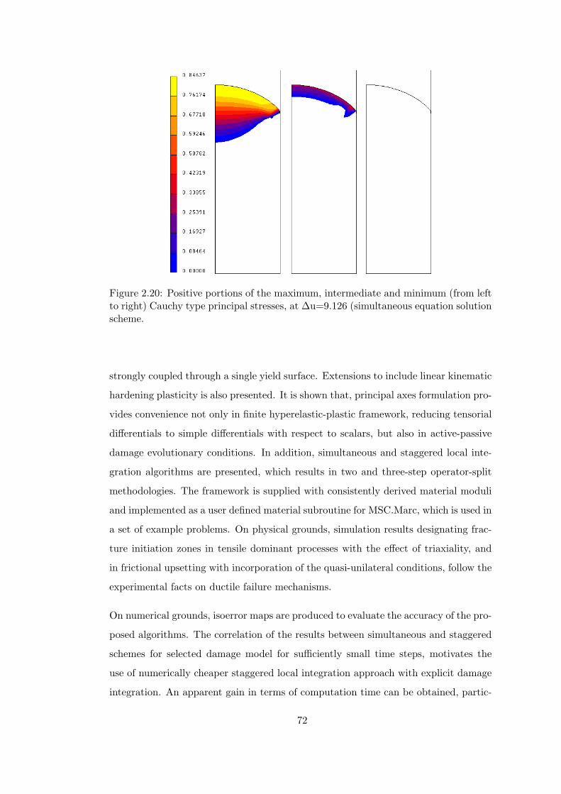
Figure 2.20: Positive portions of the maximum, intermediate and minimum (from leftto right) Cauchy type principal stresses, at ∆u=9.126 (simultaneous equation solutionscheme.
strongly coupled through a single yield surface. Extensions to include linear kinematic
hardening plasticity is also presented. It is shown that, principal axes formulation pro-
vides convenience not only in finite hyperelastic-plastic framework, reducing tensorial
differentials to simple differentials with respect to scalars, but also in active-passive
damage evolutionary conditions. In addition, simultaneous and staggered local inte-
gration algorithms are presented, which results in two and three-step operator-split
methodologies. The framework is supplied with consistently derived material moduli
and implemented as a user defined material subroutine for MSC.Marc, which is used in
a set of example problems. On physical grounds, simulation results designating frac-
ture initiation zones in tensile dominant processes with the effect of triaxiality, and
in frictional upsetting with incorporation of the quasi-unilateral conditions, follow the
experimental facts on ductile failure mechanisms.
On numerical grounds, isoerror maps are produced to evaluate the accuracy of the pro-
posed algorithms. The correlation of the results between simultaneous and staggered
schemes for selected damage model for sufficiently small time steps, motivates the
use of numerically cheaper staggered local integration approach with explicit damage
integration. An apparent gain in terms of computation time can be obtained, partic-
72

ularly in the context of explicit FE procedures, where the overall computational time
is dominantly governed by the local return mapping at integration points. This possi-
bility is investigated by the researchers for bulk metal forming simulations, conducted
with the developed subroutines for explicit commercial FE solvers in which powerful
contact algorithms are available. An apparent gain in terms of computation time can
be obtained, particularly in the context of explicit FE procedures, where the overall
computational time is dominantly governed by the local return mapping at integration
points. This possibility is investigated by the researchers for bulk metal forming simu-
lations, conducted with the developed subroutines for explicit commercial FE solvers
in which powerful contact algorithms are available.
73

CHAPTER 3
THERMO-INELASTIC FORMULATION
3.1 Introduction
In a thermo-mechanical problem, heat is produced by dissipated mechanical work in
addition to external heat sources if any exist. Produced heat is conducted/convected
over the problem domain where rate sensitivity is applicable even to rate-independent
models due to the time-dependence of heat flux, [198]. In order to solve the cou-
pled problem for deformation and temperature one has to take into account a set of
complicated mutual interactions among fields. In the absence of damage, problems
of interest in thermoplasticity often display a two sided coupling, which according to
[162] exhibits the following effects:
• The influence of the thermal field on the mechanical field
– Thermal expansion
– Temperature induced elastic softening, temperature dependence of elastic
material properties
– Temperature induced plastic softening, yield locus shrinkage
• The influence of the mechanical field on the thermal field
– Geometric coupling on heat flux
– Heat generation by plastic dissipation
– Structural elastic heating (Gough-Joule Effect)
74

In the current context, plasticity and damage accounts for the irreversible dissipative
processes. In addition to the mentioned above, conditions that must be analyzed in
the presence of damage include:
• The action of the damage field on the other mechanical fields
– Damage induced elastic softening, deteriorated elastic stiffness
– Damage induced yield locus shrinkage
• The influence of the damage field on the thermal field
– Heat generation by damage dissipation
– Damage dependent heat flux
• The influence of the thermal field on the damage field
– Direct effect through temperature dependence of the damage dissipation
functions,
– Indirect effect through reconstruction of other damage deriving mechanical
fields (e.g. triaxiality).
This highly complicated picture is the norm rather than the exception for many en-
gineering applications. In the context of isotropic damage coupled finite plasticity,
different numerical models are presented by [165], [85], [86], [87], [181], [171], [107],
[5], among others. These frameworks, however, are presented in a purely isothermal
setting. [48] presents a damage coupled finite strain thermoplastic framework utiliz-
ing Gurson damage model, whereas Lemaitre damage model is presented in [154],
[155] and [100]. These involve the hypoelastic formulations relying on objective stress
integrators. Formulations based on multiplicative framework are given in [59] where
a continuum sensitivity method is developed for porous metal plasticity using Gur-
son damage model. In the mentioned applications, the effect of damage on the heat
conduction is not reflected. However, at micro-scale the deterioration of the material
continuity through void nucleation, growth and coalescence inherently affects con-
duction quality. At the extreme where D = 1 the conduction is naturally precluded
whereas the convection on the produced free surface is due. Mathematically this is
supplied by a damage dependent heat conduction coefficient, [60].
75

Bracketing anisotropy and reducing the symmetry class to simple isotropy, the current
chapter aims to formulate a consistent thermodynamic framework for finite multiplica-
tive thermoplasticity coupled with damage which gives account for the listed mutual
effects. Recently, in the finite strain context depending on pure mechanical theory,
thermodynamics based anisotropic formulations depending on multiplicative decom-
position of metric transformation tensor are given in [31]. Frameworks with introduc-
tion of fictitious undamaged configurations are proposed by [117], [53]. [118]. Present
formulation expands on representation of the damage-coupled framework given in
[173] (which uses a dynamic explicit setup) to include thermal coupling together with
a quasi-static formulation. Finite strain kinematics utilizes multiplicative split of the
deformation gradient into elastic and plastic portions. A principal axes formulation
is used based on a hyperelastic potential quadratic in Hencky strains and nonlinear
isotropic hardening von Mises plasticity (which is typical for metals). This way, the
stress from properly articulated definition of elastic potential supplies a precise elas-
tic prediction. The total hyperelastic relations for the stress, have proved reliability
for the cases where small elastic strain assumption may fall short, like in the case of
high velocity impact and explosion, in which high elastic dilatations may be observed.
Besides, hypoelastic stress formulations lead dissipation for even elastic cycles, [196].
The treatment of scalars rather than tensors, together with the principal axes formu-
lation, serves handiness. The present formulation of finite kinematics is resolved in
eigenvectors rather than eigenbases. In eigenbases representation, the determination
of discrete eigenvalues are not required as the closed form solution for the eigenbases
is due, [161], whereas in the eigenvalue solution, eigenvalues have to be computed uti-
lizing the eigenvalue problem, [148]. In resolution of damage, conventional isotropic
Lemaitre damage model is selected, where the effective stress concept, [88] and [144],
together with strain equivalence principle, [95], form the bases.
The thermodynamic framework is formed along the same lines with [162]. Exploiting
the additivity or extensive property of the entropy, its decomposition into the elastic
and inelastic portions is postulated. It is shown that, together with temperature
dependent plastic and damage dissipation potentials, the internal variable inelastic
entropy has a natural split form in plastic and damage portions. This amounts to
a generalization of the postulated results suggested by [162] to the case of damage
76

coupling. Consequently, not only the plastic structural changes but also the damage
structural changes are consistently linked to their regarding entropies. [14] also argues
thermo-mechanical resolutions along the same lines with [162], however for anisotropic
concrete damage. An interesting irreversible thermodynamics theory is presented in
[16], where the entropy production is utilized as a metric for damage evolution, and
consequently phenomenological damage potential definitions are bypassed, unlike the
present study.
The numerical resolution of the thermo-mechanical problem is addressed as well, where
a staggered scheme with the so-called isothermal split is utilized. Accordingly, the
mechanical problem is realized under fixed temperature and the thermal problem
under fixed configuration, both utilizing the other’s result as their own boundary
conditions. Although the isothermal split is practically implemented into the exist-
ing codes and serves certain numerical advantages such as adoption of different time
scales to uncoupled mechanical and thermal steps; it, however, is, at its best, only
conditionally stable. Another staggered resolution, the adiabatic split, based on an
isentropic mechanical step, overcomes this problem of conditionality. For a detailed
analysis involving the comparison of staggered and simultaneous thermo-mechanical
resolutions, the reader may refer to [198], [162], [9], [10] and the references therein.
A covariant principal axis formulation of the same framework is given in [81]. More
recently, [34] expands the formulations and application problems to give account for
temperature dependent elastic properties. Thermoplasticity with kinematic harden-
ing is investigated in [69]. These applications exclude the void growth mechanism,
i.e. damage, and accompanying softening in metallic materials. A thermo-plastic
framework with a staggered resolution is presented in [70)] for porous plasticity. [176]
addresses the numerical consequences isothermal and isentropic split for a nonlocal
thermo-damage model. Finally, [133, pp. 637–672] supplies detailed information on
the various methodologies of the solution of thermo-mechanical problems.
Numerical solution of the post-peak responses of material models including soften-
ing regimes via finite element procedures is prone to mesh sensitivity and related
nonphysical localization. This is described as the loss of ellipticity in the context of
quasi-static problems. In this regard, for a physically admissible solution, the material
models should be enhanced with localization limiters, which keep the numerical prob-
77

lem well-posed. In the current study, strain hardening effects are in competition with
a doubly softening mechanism induced by damage and temperature. Thus, a simple
Perzyna type viscous regularization is adopted into the existing framework in the
spirit of [147] and [168]. Accordingly, the initial boundary value problem subjected to
this doubly softening mechanism is kept well-posed. The effect of devising material
rate dependence on the change of the character of the governing differential equation
is presented in [127], in which it is shown that, in the context of quasi-static problems,
the ellipticity loss is precluded by the incorporation of the viscosity and the patholog-
ical mesh sensitivity is thus healed. However, as shown in the application problems,
this localization limitation property of the viscous regularization schemes is limited
to certain deformation levels. More advanced models, such as gradient type localiza-
tion limiters, are presented, in a pure mechanical setting, by [7], [37] and [116)] for
isotropic damage models. [32] expands the nonlocal framework to anisotropic models.
Treatment of anisotropic (visco)damage coupled with (visco)plasticity can be found in
[2]. With nonlocal extensions, an isotropic Gurson damage model coupled thermo-
plastic framework is presented in [70)]. More general thermo-mechanical frameworks
with viscous and nonlocal enhancements accompanying anisotropic damage take place
in [189] and [190].
This chapter has the following outline. Local constitutive forms are derived in § 3.2
in a thermodynamic consistency. Numerical aspects, including the FE formulation of
the coupled thermo-mechanical problem, algorithmic forms and the consistent tangent
moduli are given in § 3.3. § 3.4 constructs the formulations for adiabatic conditions.
The example problems take place in § 3.5. Two damage triggering methods depending
on the imposed conditions on damage field are presented, which, to the authors knowl-
edge, haven’t been presented in the literature yet. Besides the localization prevention
characteristics of the viscous regularization in existence of two softening mechanism
are investigated. ABAQUS implementation details are presented in Appendix B.
3.2 Theory
Based on the kinematic assumptions presented in Chapter 2, and following the ratio-
nal thermodynamics approach followed by [162], the internal energy, e(Fe, ξ, ηe), is
78
postulated where ηe stands for the elastic entropy associated with the lattice and ξ
denotes the vector of strain like internal variables responsible for irreversible mech-
anisms. For thermo-mechanical applications, an additively decoupled form of total
entropy, η, with η = ηe + ηpd is claimed, utilizing its extensive property. ηpd is the
inelastic (configurational) entropy, which stands for the scalar internal variable, conju-
gate to the temperature, associated with the dissipative mechanisms such as plasticity,
hardening and damage. Through the associative evolutionary forms emanating from
conventional normality conditions together with a temperature dependent damage
dissipation potential, one ends up with a natural additive split, ηpd = ηp + ηd, where
the inelastic entropy is found as the summation of the plastic, ηp, and damage, ηd,
entropies. With this phenomenological statement, the interpretation of the evolution
of inelastic entropy is made in terms of the flow stress changes in a plastic process, and
the damage dissipation potential changes, which is a nonlinear function of the elastic
energy release rate, in a damage process, with respect to temperature. By this way,
the framework given in [162] is expanded to give account for damage induced effects.
Hence, ηp is linked to the irreversible plastic structural changes, such as dislocation
motion and lattice defects and ηd is linked to the dissipative micro-structural changes
accompanied by nucleation, growth and coalescence of micro-voids and micro-cracks.
Both of ηp and ηd do involve inputs to the total entropy which are not covered by the
inputs of the mechanical dissipation.
In the current context, the vector of strain like internal variables is defined as ξ =
α, Dt, with α and D ∈ [0, 1] being responsible for isotropic hardening and damage,
respectively. Invariance requirements for constitutive model under arbitrary rigid
body rotations on the intermediate configuration motivate the use of e(Fe, ξ, ηe) 7→
e(be, ξ, ηe), where be represents the elastic left Cauchy-Green deformation ten-
sor, with be = Fe • Fe,t. One may apply the Legendre transformation to derive,
e(be, ξ, ηe) = Ψ(be, ξ, θ) + θηe, in which Ψ(be, ξ, θ) represents the Helmholtz free
energy, which is set in terms of the absolute temperature, θ, instead of elastic entropy.
An additively decoupled form of Ψ(be, ξ, θ) reads
Ψ(be, ξ, θ) := Ψe(be, D) + Ψtd(Je, θ,D) + Ψt(θ) + Ψp(α, θ), (3.1)
where Ψe(be, D) denotes the damage affected pure elastic free energy1. Ψp(α, θ) stands1 To supply this form, for the sake of simplicity, temperature independent elastic material param-
79

for the plastic free energy blocked in the dislocations. Ψt(θ) is associated with the
purely thermal entropy. Elastic structural entropy is constructed through the thermo-
dilatational potential, Ψtd(Je, θ,D). The relations between the nominal (homogenized)
and the effective free energies follow
Ψe(be, D) = (1−D) Ψe(be), (3.2)
Ψtd(Je, θ,D) = (1−D) Ψtd(Je, θ), (3.3)
with,[F]
:= [F] /(1 − D), where[F]
and [F] are associated with the effective
and nominal forms of any tensorial or scalar quantity. Effective forms act on the
intact material subscale whereas nominal forms reflect mathematically homogenized
behavior under the influence of damage deterioration.
3.2.1 Equations of State
The second principle of thermodynamics for a thermo-mechanical problem postulates
a nonnegative difference between the local stress power and the local rate of change
of free energy. This, as a measure for the thermodynamic admissibility, supplies the
following so-called the Clausius-Duhem inequality,
0 ≤ Ω = τ : d+θ∂η
∂t− ∂e
∂t− 1
θq • g, (3.4)
where τ is the Kirchhoff stress tensor which is the work conjugate of the spatial
rate of deformation tensor, d := sym [l] , with l := ∂F/∂t • F−1 denoting the spatial
velocity gradient. q stands for the Kirchhoff type heat flux, analogous with the
weighted Cauchy stress. g is associated with the spatial gradient of θ with g := ∇θ.
This inequality can be split into two more restrictive inequalities, namely, the local
thermo-mechanical, i.e reduced Clausius-Planck form, and the conductive thermal,
i.e. Fourier Form,
Ω = Ωlthm + Ωcth ≥ 0, Ωlthm ≥ 0, Ωcth ≥ 0. (3.5)
where the respective dissipation potentials are denoted by Ωlthm and Ωcth, with
Ωlthm := τ : d + θ∂η
∂t− ∂e
∂t, (3.6)
Ωcth := −1θq • g. (3.7)
eters are assumed, µ(θ) 7→ µ, H(θ) 7→ H. For a treatment including temperature dependent elasticconstants for thermoplasticity, see [34].
80

Natural satisfaction of the condition, Ωcth ≥ 0, is supplied with (3.55) of § 3.2.5. The
remaining inequality, Ωlthm ≥ 0, postulates a stronger form of the original setup. By
making appropriate substitutions for Ωlthm and using previously postulated Legen-
dre transformation, one has,
∂e
∂t=
∂Ψ∂t
+∂θ
∂tηe +
∂ηe
∂tθ. (3.8)
Using the main inequality, (3.5.b) supplies,
0 ≤ Ωlthm = τ : d+θ
[∂η
∂t− ∂ηe
∂t
]︸ ︷︷ ︸
= ∂ηpd
∂t
−∂Ψ∂t
− ∂θ
∂tηe. (3.9)
Applying the chain rule of differentiation
∂Ψ∂t
=∂Ψ∂be
:∂be
∂t+
∂Ψ∂ξ
• ∂ξ
∂t+
∂Ψ∂θ
∂θ
∂t, (3.10)
with∂be
∂t= £vbe + l • be + be • lt, (3.11)
where £v [F] stands for the objective Lie derivative of [F] via,
£vbe = F • ∂Gp
∂t• Ft, (3.12)
in which Gp := Cp,−1 = Fp,−1 • Fp,−t, [109]. Cp is the plastic right Cauchy-Green
deformation tensor whose inverse is designated by Gp. Substituting (3.11) back into
(3.9), together with certain manipulations, one finds,
0 ≤ Ωlthm =[τ−2
∂Ψ∂be •b
e
]︸ ︷︷ ︸
=0
: d + 2∂Ψ∂be •b
e︸ ︷︷ ︸=:τ
:[−1
2£vbe • be,−1
]+ θ
∂ηpd
∂t
+[−∂Ψ
∂ξ
]• ∂ξ
∂t+[−∂Ψ
∂θ− ηe
]︸ ︷︷ ︸
=0
∂θ
∂t.
(3.13)
Accordingly following state equations are derived,
τ =∂Ψ∂be • be, ς = −∂Ψ
∂ξ, ηe = −∂Ψ
∂θ, (3.14)
where elastic entropy is found out to be the conjugate variable of the temperature. ς is
the vector of stress like internal variables which are dual with ξ, where ς = q, Y dt. q
is responsible for isotropic hardening in the form of yield locus expansion whereas Y d is
the thermodynamically formal damage conjugate variable. Substitution of the derived
81

state equations yields the following reduced dissipation inequality, whose maximization
furnishes the base for state variable evolution equations,
0 ≤ Ωlthm = τ :[−1
2£vbe • be,−1
]+[−∂Ψ
∂α
]︸ ︷︷ ︸
=:q
∂α
∂t+[−∂Ψ
∂D
]︸ ︷︷ ︸
=:Y d
∂D
∂t+ θ
∂ηpd
∂t, (3.15)
Specified additively decoupled potentials given in (3.1) result in the following explicit
representations for the state equations2,
τ = (1−D)
[∂Ψe
∂be +∂Ψtd
∂be
]• be, (3.16)
q = −∂Ψp
∂α, (3.17)
Y d = Ψe + Ψtd, (3.18)
ηe = −(1−D)∂Ψtd
∂θ− ∂Ψt
∂θ− ∂Ψp
∂θ. (3.19)
Due to its dependence on Ψtd, the definition of total Kirchhoff stress tensor gives
account for additional temperature dependent dilatational terms, compared to the
isothermal solution. Also in this setting, damage conjugate variable includes ther-
mally motivated portions, as an extension of the canonical Lemaitre damage model.
Meanwhile, the strain equivalence principle gives that the effective Kirchhoff stress,
i.e. τ = τ/(1−D), does not explicitly depend on D.
2 A remarkable fact is that, once the temperature dependence of the elasticity parameters aretaken into account, one has Ψe = Ψe(be, θ), and
ηe = −(1−D)
[∂Ψe
∂θ+
∂Ψtd
∂θ
]− ∂Ψt
∂θ− ∂Ψp
∂θ.
82

3.2.2 Equations of Evolution
The local thermo-mechanical dissipation, Ωlthm, that should be maximized, can be
split into mechanical, Ωmech, and thermal, Ωther, portions3, [47],
0 ≤ Ωlthm := τ :[−1
2£vbe • be,−1
]+ q
∂α
∂t+ Y d ∂D
∂t︸ ︷︷ ︸=:Ωmech
+ θ∂ηpd
∂t︸ ︷︷ ︸=:Ωther
. (3.20)
The evolutionary forms exploit the standard arguments of the maximization of the
inelastic dissipation, [105], where the plastic yield potential as a constraint function is
now modified to involve the damage dissipation potential as well. The hypothesis of
generalized standard materials, which proposes the existence of normality rules, [111],
applies equally valid. Accordingly, a loading function, φt, additively decoupled into
a temperature dependent plastic potential, φ, and a temperature dependent damage
dissipative potential, φd, is postulated,
φt(τ , q, Y d;D, θ) = φ(τ , q; θ) + φd(Y d;D, θ). (3.21)
Owing to the fact that the plastic flow is physically possible at undamaged material
sub-scale, the formulation of φ takes place in the effective Kirchhoff stress space.
Within the context of isotropy, associated plasticity is recovered, where the plastic
flow represented by the flow rule is coaxial with the Kirchhoff stress,
£vbe = −2γ
(1−D)∂φ
∂τ• be, (3.22)
3 Utilizing Ωmech = Ωmech,p + Ωmech,d, with,
Ωmech,p = τ :
[−1
2£vb
e • be,−1
]+ q
∂α
∂t,
and
Ωmech,d = Y d ∂D
∂t,
this form accounts for
Ωlthm + Ωmech,p + Ωmech,d ≥ 0.
which is implied by the additive decomposition η = ηe + ηp + ηd, and which is in accordance withEquation 29 of [189].
83

where γ is the single plastic multiplier. Coming to the rates of the scalar internal
variables, α, D and ηpd, one derives,
∂α
∂t= γ
∂φ
∂q, (3.23)
∂D
∂t= γ
∂φd
∂Y d, (3.24)
∂ηpd
∂t= γ
[∂φ
∂θ+
∂φd
∂θ
]. (3.25)
which are conventional, associative evolutionary rules. Since the growth of both α
and D depend on γ, damage concurrently occurs with plasticity. In the context of
inelastic dissipation maximization postulate, multi-surface damage-plasticity models,
which give account for separate plastic and damage multipliers, in the form of La-
grange multipliers, damage evolution in absence of plastic flow is possible, [75)].
Current treatment supplies the source of kinematic coupling between plasticity and
damage. Such an application has proved convenient in ductile metal damage, where
the dislocation pile-ups supply as a void nucleation source. This definition also pos-
tulates that the evolution of the inelastic entropy depends on both the plasticity and
the damage dissipation potentials, which is an expanded version of [162], in which no
damage mechanism is taken into account. It is remarkable that, one may represent
the inelastic entropy production in an additive form in terms of plastic and damage
parts as follows,
∂ηpd
∂t=
∂ηp
∂t+
∂ηd
∂t,
∂ηp
∂t= γ
∂φ
∂θ,
∂ηd
∂t= γ
∂φd
∂θ. (3.26)
For the sake of completeness, Kuhn-Tucker optimality conditions end this section.
γ ≥ 0, φ(τ , q; θ) ≤ 0, γφ(τ , q; θ) = 0. (3.27)
3.2.3 Viscous Regularization and the Penalty Method
It is a well known fact that softening regimes are prone to numerical difficulties.
These difficulties show themselves as non-uniqueness of the solution or mesh-non-
objectivity which is frequently pronounced as pathological mesh dependency. These
can be regularized, however partially, through encountering viscosity. In the context
of damage-coupled plasticity, using Perzyna type rate dependence, single surface
overstress type viscous forms are utilized by [147] and [168] among others. It is
84

notable that taking a viscous plasticity model affects the structure of the damage
evolutionary form through a single plastic potential and enforces it to have a viscous
character also. In this method, the viscoplastic multiplier, γvp , is not found via the
consistency condition, ∂φ/∂t = 0, but computed through an overstress form,
γvp =〈φ〉η
,
with 〈F〉 standing for the Macaulay brackets where 〈F〉 = 1/2 [F+ |F|]. The vis-
cosity parameter, η, should be selected as sufficiently small positive number to mimic
instantaneous plasticity with care, not to create numerical difficulties. This formu-
lation of plasticity falls in the class of penalty formulations rather than Lagrange
multiplier methods. For η 7→ 0 inviscid plasticity is recovered, whereas instantaneous
elasticity is obtained for η 7→ ∞4. From now on, the evolutionary forms are subjected
to the modification γ 7→ γvp, to involve regularizing rate effects.
3.2.4 The Temperature Evolution Equation
Following temperature evolution equation constitutes the boundary value problem for
temperature,
Cv∂θ
∂t= Ωmech − H− Jdiv
[qJ
]+ R, (3.28)
where Cv denotes the specific heat and H denotes the elastic-plastic-damage structural
heating which is related to the latent (non-dissipative) elastic and inelastic structural
changes. R and q represent the heat source and the Kirchhoff type heat flux,
respectively, both of which are omitted in adiabatic processes. The temperature evo-
lution equation can be found through the local energy balance equation, i.e. the first
principle of thermodynamics,
−Jdiv[qJ
]+ R ≥ ∂e
∂t− τ : d. (3.29)
Substituting the local thermo-mechanical dissipation definition
Ωlthm := τ : d+θ∂η
∂t− ∂e
∂t⇒ ∂e
∂t− τ : d = −Ωlthm + θ
∂η
∂t, (3.30)
4 Treatment of creep can be carried out the same setting, exploiting the equivalence of bothelastoviscoplastic and creep formulations. Creep may be seen as a special case of viscoplasticitywhere the elastic domain is null, [179].
85

and using Ωlthm = Ωmech+Ωther, where Ωther = θ[∂ηpd/∂t
], and [∂η/∂t] = [∂ηe/∂t]+[
∂ηpd/∂t], one has,
∂e
∂t− τ : d = −Ωmech + θ
[∂η
∂t− ∂ηpd
∂t
]. (3.31)
Since ηe = η − ηpd = −∂Ψ/∂θ and [∂Ψ/∂t] = τ : d − Ωmech + [∂θ/∂t] ηe, one carries
out,
θ
[∂η
∂t− ∂ηpd
∂t
]=[−θ
∂
∂θ
[τ : d− Ωmech
]]︸ ︷︷ ︸
=:H
+∂θ
∂t
[−θ
∂2Ψ∂θ2
]︸ ︷︷ ︸
=:Cv
. (3.32)
Note that, (3.32) checks with [162]. However in the preceding form, Ωmech inherently
involves damage effects. Moreover H is found as,
H = −θ
∂
∂θ
[∂Ψ∂be
]:∂be
∂t+
∂
∂θ
[∂Ψ∂α
]∂α
∂t+
∂
∂θ
[∂Ψ∂D
]∂D
∂t
. (3.33)
3.2.5 Application to a Model Problem
In this section the potentials are specified in order to derive the explicit represen-
tations of the state laws and the evolutionary equations. For elasticity, one may
postulate a deviatoric-volumetric split for the effective elastic potential, Ψe(be) =
Ψe,vol(Je) + Ψe,dev(λeA), (A = 1, 2, 3), where use of the principals of the tensor argu-
ments in representation of the isotropic tensor functions is possible,
Ψe,vol(Je) :=12
H log[Je]2, (3.34)
Ψe,dev(λeA) := µ (log[λe
1]2 + log[λe
2]2 + log[λe
3]2) (3.35)
= µ (εe,21 + εe,2
2 + εe,23 ).
with H and µ being the bulk and the shear modulus, respectively. λeA =
√beA stands
for the principal elastic stretch with the deviatoric portion represented by λeA. εe
denotes the elastic logarithmic strain tensor with principals represented by εeA. This
quadratic form in terms of Hencky measure of elastic strains although preserves
validity for a large class of materials up to moderately large deformations, [196],
does not satisfy the polyconvexity condition [102]. The deviatoric contribution of the
elastic logarithmic strain tensor and its principal components are denoted by, εe and
εeA, respectively.
86

For the plastic portion, following isotropic hardening potential is common which is
associated with a combined linear and saturation type. In the presence of thermal
coupling, this potential reads,
Ψp,iso(α, θ) =12K(θ) α2 + τ0,∞(θ)
[δ +
exp[−δα]δ
], (3.36)
with, τ0,∞(θ) := τ∞(θ) − τ0(θ), where and τ0(θ) and τ∞(θ) denote the initial and
the final yield stress of the material at temperature θ, respectively. Following [162],
linear thermal softening, with hardening softening parameter, ωh, acting on plasticity
parameters is assumed,
τ0(θ) = τ0(θ0) [1− ωh(θ − θ0)] , (3.37)
K(θ) = K(θ0) [1− ωh(θ − θ0)] ,
τ0,∞(θ) = τ0,∞(θ0) [1− ωh(θ − θ0)] .
Volumetric elastic deformation is associated with the thermal effects through the fol-
lowing thermo-dilatational potential,
Ψtd(Je, θ) = −3 H αt log[Je]Je
(θ − θ0). (3.38)
Pure thermal potential is defined as
Ψt(θ) = Cv
[(θ − θ0)− θ log
[θ
θ0
]], (3.39)
which satisfies the condition, −Cv =[∂2Ψt/∂θ2
]. These definitions let one find the
following state equation for the homogenized Kirchhoff stress,
τ = (1−D)
H
tr[ε e] − 3 αt(θ − θ0)
1− log[Je]Je
︸ ︷︷ ︸
=:p
1 + 2µ εe︸ ︷︷ ︸=:s
, (3.40)
where p = (τ1+ τ2+ τ3)/3 and s represent the temperature dependent effective Kirch-
hoff type hydrostatic stress and the deviatoric effective Kirchhoff stress tensor,
respectively. The eigenvalues of the latter is denoted by sA. Thanks to isotropy, εe
and s are coaxial thus share identical eigenbases, mA = νA⊗νA, where νA represents
the corresponding eigenvectors with (A = 1, 2, 3). As a consequence of the preceding
87

definitions, the rest of the state equations read,
q = −K(θ) α− [τ∞(θ)− τ0(θ)] [1− exp[−δα]] , (3.41)
Y d =12
H log[Je]2 + µ (εe,21 + εe,2
2 + εe,23 )− 3 H αt log[Je]
Je(θ − θ0), (3.42)
ηe =12ωhK(θ0) α2 + ωhτ0,∞(θ0)
[δ +
exp[−δα]δ
](3.43)
+(1−D)3 H αt log[Je]Je
+ Cv log[
θ
θ0
].
The damage conjugate variable, Y d, is associated with the temperature dependent
total thermo-elastic energy release rate. The expression for ηe is in accordance with
the one given in [81, Equation 70], except for the fact that it includes the damage
effect at the third term on the right hand side of equivalence. The definition of the
yield potential, which is of J2 type, is made in the effective Kirchhoff stress space in
terms of the principal values of the effective Kirchhoff stress and a two parameter
simple damage dissipation potential, chosen as a power function in Y d, is utilized for
the damage dissipation, which read,
φ(sA, q; θ) := [s21 + s2
2 + s23]
1/2 −√
23
y(q, θ) ≤ 0, (3.44)
φd(Y d;D, θ) :=a(θ)
(s + 1)1
(1−D)
[Y d
a(θ)
]s+1
, (3.45)
with y(q, θ) = [τ0(θ) − q(α, θ)] representing the hardening/softening function for
thermo-coupled conditions. A linear temperature dependence is chosen for the damage
parameter, a(θ), via
a(θ) = a(θ0) [1− ωd(θ − θ0)] . (3.46)
Consequently, with the definition of ∂φ/∂τ , the plastic flow rule can be defined,
∂φ
∂τ=
3∑A=1
nA νA ⊗ νA ⇒ £vbe = −2γvp
(1−D)
[3∑
A=1
nA νA ⊗ νA
]• be, (3.47)
where nA = ∂φ/∂τA = sA/ 2√
s21 + s2
2 + s23. It is notable that the eigenbases for the
effective and the homogenized stresses are equivalent, i.e. νA ⊗ νA ≡ νA ⊗ νA. The
rates of the scalar strain like variables, α and D, read,
∂φ
∂q= −
√23
⇒ ∂α
∂t= −γvp
√23,
∂φd
∂Y d=
1(1−D)
[Y d
a(θ)
]s
⇒ ∂D
∂t= γvp 1
(1−D)
[Y d
a(θ)
]s
.
(3.48)
88
Following similar arguments, the growth of the plastic portion of the inelastic entropy
reads,
∂ηp
∂t= γvp
√23
[ω0τ0(θ0)− ωhq(α, θ0)] , (3.49)
which is identical to [162]. The growth of the inelastic entropy associated with damage
is,
∂ηd
∂t= γvp 1
(1−D)
[Y d
a(θ)
]s [ωda(θ0)
Y d
a(θ)− 3 H αt log[Je]
Je
]. (3.50)
The details of these derivations are given in Appendix C. The expressions add up
to the rate of total inelastic entropy production, ∂ηpd/∂t, utilizing (3.26). The sec-
ond principle of thermodynamics places a restriction on the definition of the thermal
dissipation via Ωther = θ[∂ηpd/∂t
]≥ 0. Accordingly one may suggest two stronger
inequalities, such as ∂φ/∂θ ≥ 0 and ∂φd/∂θ ≥ 0. The former is naturally satisfied,
where in the view of (3.37) thermal softening of the plastic potential, is addressed5.
This condition, also named as the yield locus contraction with temperature, reflects
the experimental evidences.
Following simplification, introduced in [162], is invariably valid for the current damage-
coupled plasticity,
Ωmech,p = γvp
√23τ0(θ),
where the details of this derivation can be found in Appendix C. Together with the
definition of damage dissipation,
Ωmech,d := Y d ∂D
∂t︸︷︷︸γ ∂φd
∂Y d
= γvp a(θ)(1−D)
[Y d
a(θ)
]s+1
, (3.51)
5 For two-surface damage coupled plasticity models, where independent plasticity-damage evo-lution can be observed, analogical to the plasticity, damage softening amounts for the thermal con-traction of the separately defined damage surface which is related to the free surface energy of themicro-void/micro-crack formation.
89

one may find the following total mechanical dissipation6, Ωmech,
Ωmech = Ωmech,p + Ωmech,d = γvp
[√23τ0(θ) +
a(θ)(1−D)
[Y d
a(θ)
]s+1]
. (3.52)
This expression has a crucial importance in the current thermo-inelastic framework.
Besides constituting the heat source, it also accounts for the term that is used in
linearization of the weak form of the thermal problem.
Coming to the time sensitive thermal dissipation analysis, a damage affected potential,
Φ, is utilized, [60],
Φ = (1−D)Φ; Φ = −12k g • g, (3.53)
where k is the (isotropic) heat conduction coefficient. This equation eventually defines
the following damage affected heat flux vector, which is in the form of the classical
Fourier’s linear heat flow equation,
q = −∂Φ∂g
= −(1−D)k g ⇒ q = −(1−D)k g. (3.54)
Substituting the values in the conductive thermal Fourier inequality, supplies,
Ωcth = −1θq • g = (1−D)
1θk g • g ≥ 0. (3.55)
It is clearly seen that this inequality is unconditionally satisfied for a positive heat
conduction coefficient, k> 0.
3.3 Numerical Implementation
3.3.1 FE Formulation of the Coupled IBVP
Let P := τ • F−t stand for the first (unsymmetric) Piola-Kirchhoff stress and
Q := F−1 • q stand for the heat flux of equivalent type, analogically. Utilizing the6 In the presence of damage, since Ωmech,d Ωmech,p, it may be advocated that, Y d ∂D/∂t ≈ 0.
With this cancelation one has,Ωmech ≈ Ωmech,p.
Also, following the experimental observations of [183], for instantaneous plasticity, one may constructa modified plastic mechanical dissipation, Ωmech 7−→ Ωmech,p, in terms of the plastic power,
Ωmech,p := κ
[γvp
√2
3y(q, θ)
].
where the so-called Taylor-Quinney empirical constant, κ ∈ [0, 1], defines the extent of the plasticpower which is defined as the plastic dissipation. κ is commonly selected in the range 0.85 ≤ κ ≤ 0.95.
90
Piola transform, one has Jdiv [q/J ] 7→DIV[Q] and Jdiv [τ/J ] 7→DIV[P] , with J =
det[F]. The primary unknowns of the thermo-mechanical problem, ϕ,v, θt , with v
denoting the velocity vector, are resolved at the global solution stage by considering the
following coupled differential equation set constructed at the reference configuration,∂ϕ/∂t− v
DIV [P] + ζ − ρ0v
Cv [∂θ/∂t]− Ωmech + H + DIV [Q]−R
= 0. (3.56)
Apart from the trivial velocity vector definition given in the first row; in a residual
setting, the second and third rows stand for the local equation of motion and the first
law of thermodynamics, which supplies the equation for thermal condition. v is the
acceleration vector and ρ0 is the referential density. ζ denotes the body forces. The
boundary conditions for the problem can be listed as follows,
ϕ = ϕ at ∂Bϕ;
θ = θ at ∂Bθ;
T = P •N at ∂Bσ;
Q = Q •N at ∂Bq;
∂Bϕ ∩ ∂Bσ = ∅;
∂Bθ ∩ ∂Bq = ∅;
∂Bϕ ∪ ∂Bσ = ∂B.
∂Bθ ∪ ∂Bq = ∂B.
(3.57)
with N being the outward unit normal to the boundary, ∂B, in the reference con-
figuration ∂Bϕ ⊂ ∂B and ∂Bθ ⊂ ∂B denote the parts of the boundary on which
the Dirichlet boundary conditions are specified with the prescribed displacements,
ϕ, and temperatures, θ, respectively. With the prescribed tractions, T, and the out-
ward normal heat flux, Q, Neumann type boundary conditions respectively act on
the boundary parts ∂Bσ ⊂ ∂B and ∂Bq ⊂ ∂B. The conditions satisfied on these
boundary parts are given in (3.57). In the current context, temperature increase is
merely associated with the mechanical dissipation due to irreversible processes such
as plasticity and damage. Accordingly, the heat source and the temperature varia-
tions due to elastic loading are omitted, by canceling R and H respectively, to give
Cv [∂θ/∂t]− Ωmech+DIV[Q] = 0.
(3.56) can be solved in a monolithic or a staggered manner. Monolithic scheme stands
for concurrent satisfaction of the equation set to describe the unknowns, where the
system is solved in a fully coupled manner. For this approach, see e.g. [8] and [162].
For the simultaneous solution of the global problem, consequent numerically costly
tangent stiffness matrix of thermoplasticity is usually not symmetric. Besides since
the difference of the orders of the thermal and mechanical problems, it is not well-
91

conditioned and needs post processing. In the staggered approach, the coupling is
split into mechanical and thermal branches and corresponding equations are solved
with successive decrease of mechanical and thermal residuum, where the linear mo-
mentum and the energy conservation requirements are satisfied, respectively. If the
former mechanical step is realized under constant temperature, then the split is called
an isothermal split. The isothermal staggered approaches are numerically cheaper at
the expense of numerical instability risk. Unconditionally stable algorithms may be
produced by following an isentropic mechanical step, in which the total entropy is held
constant. The code may take advantage of using different time scales for the split me-
chanical and thermal steps which is not possible with monolithic approaches. Details
of the staggered split algorithms may be found in [162] and the follow-up studies [198],
[9], [10]. For kinematic hardening thermoplasticity, staggered approach is utilized by
[69]. Similar generalizations of the staggered approach to damage involved analysis
can be found in [174] and [70)]. It should be noted that, the quadratic convergence
quality of the Newton-Raphson scheme is preserved only for the simultaneous ap-
proach, whereas the staggered algorithm does provide only super-linear convergence,
[162], [198].
3.3.1.1 Staggered Solution Scheme
In solution of the above problem, an isothermal staggered solution scheme is followed,
where an isothermal mechanical step is followed by a thermal step on fixed configura-
tion.
Mechanical Step For the mechanical problem, the equation is modified as follows
in order to preclude the temperature evolution,∂ϕ/∂t− v
DIV [P] + ζ − ρ0v
Cv [∂θ/∂t]
= 0, (3.58)
Following a Galerkin approach, both sides are multiplied by a sufficiently smooth
virtual displacement field, ηu, and integrate at the reference configuration. Applying
integration by parts followed by the divergence theorem gives the following internal
92

part of the mechanical weak statement,
gintηu
(ηu;ϕ) =∫
B0
τ : [gradηu]sym dV, (3.59)
Linearization of the internal virtual work in the direction of displacement increment
u, i.e. Dg(ϕ,ηu)[u] , reads,
Dgintηu
(ηu;ϕ)[u] :=ddε
∣∣∣∣ε=0
gintηu
(ηu;ϕ + εu). (3.60)
Time discrete forms of the above split at the quasi-static limit with, ρ0 7→ 0, is
constructed through a backward-Euler scheme. In the following, [F]n and [F]n+1
give the definitions of any variable denoted by [F], at time tn and tn+1 respectively.[F]n+1
stands for the regarding definition at the end of the isothermal mechanical
step. It is assumed that the state variables at time tn are known and using the
deformation and temperature computed at ∆t = tn+1 − tn, through a split scheme,
the state at time tn+1 is sought for. Accordingly, the isothermal mechanical step
realized under constant temperature, θn+1 7→ θn, reads
ϕn+1 −ϕn − un+1
DIV[Pn+1
]+ ζn+1
θn+1 − θn
= 0. (3.61)
Consequently, one carries out the following linearization, for the internal part of the
mechanical weak form,
KMM (ηu,un+1) := Dgintηu
=∫
B[gradηu]sym : cMM,n+1 : [gradun+1]
sym dV
+∫
Bgradηu • τn+1 • gradun+1 dV,
(3.62)
which gives the isothermal stiffness matrix, with the assembly following a spatial
discretization. On the right hand side, the first term is due to material stiffness and
the second term is due to geometric stiffness. A consistent derivation of cMM,n+1,
the spatial material tangent matrix, is vital for quadratic convergence quality of the
Newton-Raphson method. Together with the solution of this step, appropriate
updates are realized to give, ben, ξn, θn 7→
be
n+1, ξn+1, θn+1
.
93

Thermal Step After isothermal mechanical convergence is supplied, the thermal
step is solved for v
v
Cv [∂θ/∂t]− Ωmech + DIV [Q]
= 0, (3.63)
Analogically to the mechanical problem under fixed temperature, the weak statement7
for the thermal problem can be carried out by multiplying both sides of the thermal
equation with a continuous temperature field, η%. Following similar steps as given
in the preceding equations, the weak statement for the internal part of the energy
balance is carried out,
gintη%
(η%; θ) =∫
Bη%Cv
∂θ
∂tdV −
∫B
η%ΩmechdV +∫
Bη% • k∇θ dV. (3.64)
This expression is consistently linearized in the direction of temperature change %, to
give
Dgintη%
(η%; θ)[%] :=ddε
∣∣∣∣ε=0
gintη%
(η%; θ+ε%). (3.65)
Introducing the time discretization for the thermal step at fixed configuration, together
with backward-Euler method, one has,ϕn+1 − ϕn+1
vn+1 − vn+1
Cv
[θn+1 − θn+1
]/∆t− Ωmech
n+1 + DIV [Qn+1]
= 0. (3.66)
Together with this setting, the linearization of the internal part yields,
KTT (η%, %n+1) := Dgintη%
=∫
Bη%
[Cv
∆t−
∂Ωmechn+1
∂θn+1
]%n+1 dV
+∫
B∇η% • k∇%n+1 dV,
(3.67)
where dΩmechn+1 /dθn+1 =: cTT,n+1 is called the thermo-inelastic coupling modulus. The
derivation of this term is crucial for application of the Newton-Raphson scheme for
the thermal portion of the problem. At this step, the variable update is realized with,be
n+1, ξn+1, θn+1
7→be
n+1, ξn+1, θn+1
.
7 It should be noted that, for an adiabatic case which is assumed for processes taking placein a very short time duration, the heat source and the heat dissipation through conduction areomitted. Consequently, the thermal resolution can be made at material level, at an expense of anincreased dimension of the local unknowns array. This is conducted utilizing the strong form of theenergy balance equation without a need for tracking a Galerkin approach. The usual trend is theapplication of the backward-Euler method in the integration of the temporal evolutionary forms.
94

Throughout the preceding global solution scheme, switching between the split prob-
lems, mutual effects of thermal and mechanical fields on each other are reflected.
Accordingly temperature change induced by inelastic dissipative mechanisms such
as plasticity and damage are taken into account as well as softening and expansion
induced by temperature. Besides heat conduction is affected by deformation and
damage.
3.3.2 Return Mapping
Update of the state variables with local integration follows a two-step operator-split
with a simultaneous plastic/damage correction for a given elastic prediction. Using a
strain driven process, elastic trial left Cauchy-Green deformation tensor, b e, tri, can
be defined at time tn+1, making use of relative deformation gradient tensor at current
step, i.e. fn+1, with fn+1 = Fn+1 •F−1n , and elastic left Cauchy-Green deformation
tensor of the previous step, i.e. b en, as follows,
b e, trin+1 = fn+1 • b e
n • f tn+1; where b e, tri
n+1 =3∑
A=1
λe, tri, 2n+1, A νtri, A
n+1 ⊗ νtri, An+1 . (3.68)
Construction of the algorithmic counterpart of the continuum equations and applying
the exponential mapping approximation for flow rule integration, utilizing the coaxi-
ality of the plastic flow and the elastic trial state, yields the following plastic-damage
correction on trial elastic principal strains, where the strain corrections in the form of
the principal plastic strain increments, ∆ε pn+1, A, are defined as follows,
ε en+1, A = ε e, tri
n+1, A −∆γ
(1−Dn+1)∂φ
∂τA
∣∣∣∣∣n+1︸ ︷︷ ︸
∆ε pn+1, A
, (3.69)
with ∆γ = ∆t γvpn+1. For α and D, implicit backward-Euler method yields,
αn+1 = αn +
√23
∆γ , (3.70)
Dn+1 = Dn + ∆γ1
(1−Dn+1)
[Y d
n+1
a(θn+1)
]s
. (3.71)
The components of the inelastic entropy also exploit the backward-Euler method.
Accordingly the plastic portion reads,
ηpn+1 = ηp
n + ∆γ
√23
[ω0τ0(θ0)− ωhq(αn+1, θ0)] , (3.72)
95

and the damage portion reads,
ηdn+1 = ηd
n + ∆γ1
(1−Dn+1)
[Y d
n+1
a(θn+1)
]s [ωda(θ0)
Y dn+1
a(θn+1)− 3 H αt log[Je
n+1]Je
n+1
],
(3.73)
which add up to ηpdn+1 = ηp
n+1 + ηdn+1. It is remarkable that, the local integration
expressions for ηpn+1 and ηd
n+1have explicit representations in ∆γ and Dn+1. Thus,
setting the inelastic entropy as an additional internal variable does not complicate the
local integration scheme and conventional finite thermoplastic algorithmic structure
presented in [162], even for damage-coupled conditions. Resultant plastic/damage
correction of principal Kirchhoff stresses yield,
τn+1, A = τ trin+1, A − 2µ
∆γ
(1−Dn+1)nn+1, A, with τ tri
n+1, A = p + s trin+1, A. (3.74)
Plastic potential, which forms the constraint condition reads,
φn+1 := ‖sn+1‖ −√
23
y (qn+1, θn+1) = 0. (3.75)
3.3.2.1 Solution of Equations of Local Integration
Following [166], local governing equations collected so far can be reduced, particularly
for the chosen yield criterion, making use of the substitution, sn+1, A = ‖sn+1‖ nn+1, A,
and exploiting the condition of collinear flow and the trial Kirchhoff stress tensor,
finally, representing the hardening/softening function definition in terms of the plastic
multiplier, to reach,
rn+1(xn+1) =
√23
[τ0(θn+1) + K ′(αn +
√23
∆γ , θn+1)
]−∥∥s tri
n+1
∥∥+ 2µ∆γ
(1−Dn+1)+
η
∆t∆γ
Dn+1 −Dn −∆γ1
(1−Dn+1)
[Y d
n+1
a(θn+1)
]s
, (3.76)
where rn+1 = rn+1(xn+1) = 0. In above, −q = K ′ (α, θ) = ∂K (α, θ) /∂α|θ is utilized.
The array of unknowns is represented by xn+1 = ∆γ, Dn+1t. (3.76) can be treated
with the standard Newton-Raphson solution scheme. Accordingly, the linearized
version of the equations is given as drn+1 = Drn+1•dxn+1, where Drn+1 denotes the
96

Jacobian of the system which reads,
Drn+1 =
∂r1, n+1
∂∆γ
∂r1, n+1
∂Dn+1∂r2, n+1
∂∆γ
∂r2, n+1
∂Dn+1
, (3.77)
where the component derivations are given in the Appendix C. Using Dr−1n+1•drn+1 =
dxn+1, the solution for xn+1, which constitutes the local return mapping realized at
each Gauss point, can be carried out with the following iterative scheme,
x(k+1)n+1 = x(k)
n+1 − δ(k) Dr−1, (k)n+1 • r(k)
n+1, (3.78)
where δ(k) ∈ (0, 1] is the proper line-search parameter.
3.3.3 Algorithmic Tangent Matrices
For the monolithic solution of the global equilibrium problem of coupled thermo-
mechanical analysis, one has,
rn+1 = rn+1(xn+1) = 0; xn+1
εn+1, A
θn+1
∆γ
Dn+1
. (3.79)
where ∆γ = ∆γ(εn+1, θn+1) and Dn+1 = Dn+1(εn+1, θn+1). A mechanical-thermal
staggered approach introduces following simplifications into the solution scheme.
3.3.3.1 Mechanical Pass
Mechanical pass is realized under constant temperature, where θn+1 = θ which results
in ∆γ = ∆γ(εn+1)|θ=θ and Dn+1 = D(εn+1)|θ=θ. For this stage,
rn+1 = rn+1(xn+1) = 0; xn+1
εn+1, A
∆γ
Dn+1
∣∣∣∣∣∣∣∣∣θn+1=θ
. (3.80)
with the vanishing total differential, dr = 0, yieldsd∆γ
dεn+1, AdDn+1
dεn+1, A
= −Dr−1n+1 •
∂r1, n+1
∂εn+1, A∂r2, n+1
∂εn+1, A
. (3.81)
97

Accordingly the computation of the mechanical tangent matrix, in the form of the
spatial elastoplastic-damage tangent moduli, [161], reads
cMM, ijkl = 2FiI FjJ FkK FlL CIJKL, (3.82)
which is a push-forward transformation of Lagrangian constitutive moduli, CIJKL,
which is defined by,
CIJKL =∂SIJ
∂CKL, (3.83)
where S = F−1 • τ •F−t, is the second Piola Kirchhoff stress tensor, i.e. the pull-
back transform of the Kirchhoff stress tensor and C is the right Cauchy-Green
deformation tensor. An explicit representation of cMM,n+1 can be given as,
cMM,n+1Jn+1 =3∑
A=1
3∑B=1
aepdn+1, AB νtri, A
n+1 ⊗ νtri, An+1 ⊗ νtri, B
n+1 ⊗ νtri, Bn+1
−3∑
A=1
2(1−D)τn+1, Aνtri, An+1 ⊗ νtri, A
n+1 ⊗ νtri, An+1 ⊗ νtri, A
n+1
+3∑
A=1
3∑B=1A6=B
ϑABνtri, An+1 ⊗ νtri, B
n+1 ⊗ νtri, An+1 ⊗ νtri, B
n+1 .
(3.84)
Utilizing the condition dεn+1 7→dε e, trin+1 , aepd
n+1, AB is posed as the following 3×3 matrix,
aepdn+1, AB =
dτn+1, A
dεe, trin+1, B
. (3.85)
Since the mechanical step in the staggered approach assumes
τn+1(εn+1, θn+1,∆γ (εn+1, θn+1), D(εn+1, θn+1))
7→ τn+1(εn+1,∆γ (εn+1), D(εn+1))|θ=θ ,(3.86)
the computation of aepdn+1, AB requires the following chain rule of differentiation,
dτn+1, A
dεe, trin+1, B
=∂τn+1, A
∂εe, trin+1, B
+∂τn+1, A
∂∆γ
d∆γ
dεe, trin+1, B
+∂τn+1, A
∂Dn+1
dDn+1
dεe, trin+1, B
, (3.87)
where the details of the derivation are given in Appendix C and the definitions for
d∆γ/dεtrin+1, B and dDn+1/dεtri
n+1, B require (3.81). The designation of ϑAB is given as
ϑAB = 2τn+1, Aλe, tri, 2
n+1, B − τn+1, Bλe, tri, 2n+1, A
λe, tri, 2n+1, A − λe, tri, 2
n+1, B
, (3.88)
which suffers from singularity or ill-conditioning, for equal or nearly equal eigen-
values, respectively, where λe, trin+1, A − λe, tri
n+1, B 7→ 0. [130, pp. 338–341] includes an
98

analytical treatment of such cases in the context of finite elasticity materializing
L’Hospital rule. Accordingly, as also shown in [22, pp. 138–138, p. 202], for
λen+1, A = λe
n+1, B, the definition of ϑAB boils down to ϑAB = 2µ − 2τn+1, A. How-
ever, for inelasticity, the application of the L’Hospital rule is not straightforward
and requires significant computational time. Thus, numerical perturbation technique
serves an efficient substitute. Consequently, equal or numerically close eigenvalues
with, λe, trin+1, A ' λe, tri
n+1, B, are perturbed with a perturbation factor8, δ 1, which gives
λe, trin+1, A 7→ (1 + δ) λe, tri
n+1, A, λe, trin+1, B 7→ (1 − δ) λe, tri
n+1, B, and for volumetric consistency
λe, trin+1, C 7→ 1/[(1 + δ)(1− δ)]λe, tri
n+1, C , [119].
3.3.3.2 Thermal Pass
Coming to the second pass, the configuration is held fixed, εn+1, A = εA, which results
in ∆γ = ∆γ(θn+1)|ε=ε and Dn+1 = D(θn+1)|ε=ε . Consequently one has,
rn+1 = rn+1(xn+1) = 0; xn+1
θ
∆γ
Dn+1
∣∣∣∣∣∣∣∣∣εn+1, A=εA
. (3.89)
Analogous to the mechanical step, exploitation of the condition, dr = 0, reads,d∆γ
dθn+1dDn+1
dθn+1
= −Dr−1n+1 •
∂r1, n+1
∂θn+1∂r2, n+1
∂θn+1
. (3.90)
It should be noted that, in both the mechanical pass and the thermal pass the internal
variables are changing. The thermal portion is due only if there exists plastic flow and
induced damage. Accordingly the Jacobian for the thermal problem, cTT , becomes,
cTT,n+1 :=dΩmech
n+1
dθn+1, (3.91)
where the mechanical dissipation at the current increment is,
Ωmechn+1 =
∆γ
∆t
√23τ0(θn+1) +
a(θn+1)(1−Dn+1)
[Y d
n+1
a(θn+1)
]s+1 . (3.92)
Since the thermal step is realized under fixed configuration, one assumes,
Ωmechn+1 (εn+1, θn+1,∆γ (εn+1, θn+1), D(εn+1, θn+1))
7→ Ωmechn+1 (θn+1,∆γ (θn+1), D(θn+1))
∣∣∣ε=ε
.(3.93)
8 δ=1.0e-12 constitutes a reasonable assumption.
99

Accordingly one has,
cTT,n+1 :=∂Ωmech
∂θn+1+
∂Ωmech
∂∆γ
d∆γ
dθn+1+
∂Ωmech
∂Dn+1
dDn+1
dθn+1. (3.94)
The details of the derivation are given in Appendix C and the definitions for d∆γ/dθn+1
and dDn+1/dθn+1 require (3.90). This concludes the numerical setup.
3.4 Adiabatic Conditions
For processes which takes place in very small time zones, such as high velocity impact
or explosion, heat cannot find time to be conducted over the problem domain. Besides
large dilatational changes may occur due to high pressures, [196], which makes use
of total hyperelastic stress formulation more reasonable compared to hypoelasticity.
When the heat flux is omitted, system can be modeled under adiabatic conditions.
Accordingly, since no boundary value problem for temperature is due, the heat equa-
tion can be solved in material level. The only difference is that the local equations
become a bit more rigorous, [133]. Accordingly, the reduced set of two local equations
is increased to three, to become,
rn+1 = rn+1(xn+1) =
√23 τ0(θn+1) + K ′(αn +
√23 ∆γ )
−∥∥s tri
n+1
∥∥+ 2µ ∆γ(1−Dn+1)
Dn+1 −Dn −∆γ 1(1−Dn+1)m
(Y d
n+1
S
)s
θn+1 − θn − 1ρc∆t χ(ρwn+1)
; (3.95)
xn+1 =
∆γ
Dn+1
θn+1
. (3.96)
where the solution of simultaneous equations require a systematic application of the
Newton-Raphson method where
Drn+1 =
∂r1, n+1
∂∆γ
∂r1, n+1
∂Dn+1
∂r1, n+1
∂θn+1∂r2, n+1
∂∆γ
∂r2, n+1
∂Dn+1
∂r2, n+1
∂θn+1∂r3, n+1
∂∆γ
∂r3, n+1
∂Dn+1
∂r3, n+1
∂θn+1.
(3.97)
It should be noted that, for high velocity processes, such as machining or impact
and penetration problems, strain rate dependence should be involved in the material
100

formulation. Accordingly, strain rate hardening is taken into account. As a conse-
quence, the macroscopic material behavior gives account for a competing mechanism
in between strain hardening, strain rate hardening, thermal softening and damage
softening. A damage coupled version of the Johnson-Cook model, [84], which is
an expansion of already utilized hardening/softening function, y(q, θ), to give account
for the thermal and strain rate effects is a widely used alternative for this choice9.
In the current context, to include strain rate effects, previously presented harden-
ing/softening form can be modified to involve strain rate hardening effects as follows,
y(q, θ) = [τ0(θ)− q(α)][1 + Clog
[α
α0
]] [1− (θ − θ0)
(θm − θ0)
], (3.98)
where C is a material parameter scaling the strain rate effect. α0 denotes the ref-
erence plastic strain rate. θ0 and θm represent reference and melting temperatures,
respectively.
3.5 Application Problems
Preceding algorithmic resolutions are implemented as ABAQUS subroutines where
the implementation details are included in Appendix B. In what follows, a set of
example problems solved with these subroutines are given.
3.5.1 Necking of an Axi-symmetric Bar
Necking of an axi-symmetric bar is investigated in the context of damage-coupled
thermoplastic framework. Contrary to the common idea, in the FE simulations with
a typical free contracting (shear-free grip conditions) tensile test specimen of a certain
gauge length, central refinement of the mesh does not suffice to transform the bifurca-
tion problem, where the necking can emanate at any section, to a limit load problem.
This is due to the fact that, necking emanation requires the break up of the stress
uniformity. For this purpose, two necking triggering methods widely used in the liter-
ature are the geometric imperfection method and the thermal triggering method. The
9 Such an approach is utilized by many researchers, see e.g. [28] and [29], for an applicationon a projectile penetration into steel plate problem. Another application for the Johnson-Cookmodel may be given as the hard machining simulations, where large strains, high strain rates andhigh temperatures are experienced, see e.g. [66] and [67].
101
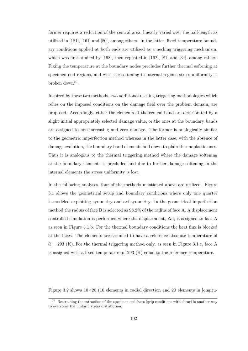
former requires a reduction of the central area, linearly varied over the half-length as
utilized in [181], [161] and [80], among others. In the latter, fixed temperature bound-
ary conditions applied at both ends are utilized as a necking triggering mechanism,
which was first studied by [198], then repeated in [162], [81] and [34], among others.
Fixing the temperature at the boundary nodes precludes further thermal softening at
specimen end regions, and with the softening in internal regions stress uniformity is
broken down10.
Inspired by these two methods, two additional necking triggering methodologies which
relies on the imposed conditions on the damage field over the problem domain, are
proposed. Accordingly, either the elements at the central band are deteriorated by a
slight initial appropriately selected damage value, or the ones at the boundary bands
are assigned to non-increasing and zero damage. The former is analogically similar
to the geometric imperfection method whereas in the latter case, with the absence of
damage evolution, the boundary band elements boil down to plain thermoplastic ones.
Thus it is analogous to the thermal triggering method where the damage softening
at the boundary elements is precluded and due to further damage softening in the
internal elements the stress uniformity is lost.
In the following analyses, four of the methods mentioned above are utilized. Figure
3.1 shows the geometrical setup and boundary conditions where only one quarter
is modeled exploiting symmetry and axi-symmetry. In the geometrical imperfection
method the radius of face B is selected as 98.2% of the radius of face A. A displacement
controlled simulation is performed where the displacement, ∆u, is assigned to face A
as seen in Figure 3.1.b. For the thermal boundary conditions the heat flux is blocked
at the faces. The elements are assumed to have a reference absolute temperature of
θ0 =293 (K). For the thermal triggering method only, as seen in Figure 3.1.c, face A
is assigned with a fixed temperature of 293 (K) equal to the reference temperature.
Figure 3.2 shows 10×20 (10 elements in radial direction and 20 elements in longitu-
10 Restraining the extraction of the specimen end faces (grip conditions with shear) is another wayto overcome the uniform stress distribution.
102

Figure 3.1: Geometry and the boundary conditions for the tensile tests.
dinal direction) mesh composed of element CAX4T, which is a 4-node axi-symmetric
thermally coupled quadrangular element with bilinear displacement and temperature
interpolations. For the central damage deterioration method (hereafter damage trig-
gering type 1), an initial nonzero damage field, smoothly varied over a certain length, is
introduced at the central zone. Accordingly, the regions numbered with n = 1, 2, 3, 4, 5
in Figure 3.2.a are deteriorated by an initial damage of, D = 2(1−n) × 10−6. The rest
of the domain has zero initial damage. For the necking triggering method which relies
on the imposed damage conditions at support regions (hereafter damage triggering
type 2), the Gauss points at the elements of zone 6, seen in Figure 3.2.b, are selected
as purely thermoplastic; that is to say, uncoupled to damage.
Figure 3.2: The regions, on 10x20 mesh, on which the damage conditions are imposed,for regarding necking triggering methods.
103

The material parameters used in the analyses are given in Table 3.1, where for mere
thermoplasticity the damage deterioration effect is cancelled.
Table 3.1: Material parameters for the example problem.
Parameter Symbol Magnitude UnitBulk modulus H 164.206 GPaShear modulus µ 80.1938 GPaFlow stress τ0 0.450 GPaSaturation stress τ∞ 0.715 GPaLinear hardening K 0.12914 GPaHardening exponent δ 16.93 -Density ρ 7.8×10⁹ Ns2/mm2
Damage multiplier a 0.1 -Damage exponent s 1.0 -Coefficient of thermal expansion αt 1×10⁻⁵ K−1
Conductivity k 45.0 N/sKSpecific capacity Cv 0.46×109 mm2/s2KHardening softening wh 0.002 K−1
Damage softening wd 0.002 K−1
Figure 3.3.a, b, c and d, respectively show the resultant deformed mesh profiles and
the damage contours of the geometric imperfection, thermal triggering, damage trig-
gering type 1 and type 2 methods for ∆u=6 (mm). Starting with, it can be observed
that, proposed necking triggering methods are capable of successfully developing the
neck by means of breaking up the stress uniformity over the problem domain. Central
damage accumulation is due for all of the models. Maximum radial thinning occurs in
the geometric imperfection method with 3.61 (mm) where the minimum occurs in the
damage triggering type 1 with 2.38 (mm). Specimens belonging to thermal triggering
and damage triggering type 2 methods experience a thinning of 3.07 (mm) and 2.07
(mm), respectively. The differences in the radial reductions are accompanied by differ-
ent central damage intensities. As expected, maximum damage accumulation is seen
in the geometric imperfection method. The rest follows the order of the magnitude of
the experienced radial reductions, which changes the effective stress contributions to
damage accumulation considerably.
104

Figure 3.3: Contour plots of the damage distribution at ∆u=6, a) Geometric im-perfection method, b) Thermal triggering method, c) Damage triggering type 1, d)Damage triggering type 2.
Figure 3.4.a and b show, respectively, the resultant load-displacement and central
temperature increase history curves. Due to considerable initial central area loss in the
geometric imperfection method, regarding load values of the load-displacement curve
follows a considerably lower trend compared to the other cases. Besides, the peak is
reached at an earlier displacement state. The latest peak is reached by the damage
triggering type 1 where the given initial centrally distributed damage is considerably
small. These results are compatible with the maximum and minimum central thinning
of the geometric imperfection and damage triggering type 1 methods, illustrated in
Figure 3.3. These results are in accordance with the radial thinning values given.
The model with the earlier neck emanation experiences further radial thinning and
damage accumulation for a given time at the domain of post peak response. The
slopes of the central temperature history curves experience an increase at the point
where the peak load response is reached. Besides the apparent shift of the bifurcation
points among the curves of different necking triggering methods, the similarity of the
105

post peak trends of both the load-displacement diagrams and the temperature history
diagrams is noteworthy.
Figure 3.4: History plots for damage-coupled axi-symmetric necking problem, a) Load-displacement curves, b) Temperature increment evolution at center.
3.5.2 Localization of a Plane Strain Strip
This part is composed of two case studies based on tension of a plane strain strip.
Initially a validation study is performed which relies on the comparison of the current
thermoplastic material model with the built in model in ABAQUS. Then, the obser-
vation of mesh dependence in the localization of deformation and damage together
with the investigation of the performance of the viscous regularization take place.
For both of the problems, the geometry, displacement and thermal boundary condi-
tions are the same as those in the previous section (Figure 3.1) where in the current
case the quarter is assumed for a plane strain case. Unless otherwise stated, the ma-
terial parameters are the ones given in Table 3.1. Element CPE4T is used, which is
4-node plane strain thermally coupled quadrilateral with bilinear displacement and
temperature interpolations. In the models thermal triggering method is utilized.
106

3.5.2.1 Validation of the Thermoplastic Code
Mere heat source is assumed to be the plastic work with the Taylor-Quinney em-
pirical constant as, χ = 0.90. Damage evolution is bypassed for this set of analyses.
In two additional analyses Perzyna type viscous regularization11 is utilized with
η = 500 and η = 1000. A fixed 10×20 mesh is used.
The load-displacement and the central temperature increment history plots are given
in Figure 3.5.a and b respectively. As seen the curves of the ABAQUS built-in model
which utilizes the corotational formulation and current hyperelastic thermoplastic
results are in perfect correlation. The effect of viscosity is also illustrated in the plots.
The abrupt loss in the load carrying capacity together with necking is precluded in
the viscously regularized solutions.
Figure 3.5: History plots for thermoplastic plane strain strip tension problem, a)Load-displacement curves, b) Temperature increment evolution at center.
In Figure 3.6.a, b, c and d deformed meshes together with temperature contour plots
can be seen. Figure 3.6.a and b belong to ABAQUS built-in model and present
thermoplastic model respectively. Figure 3.6.c and d respectively belong to the results
for thermo-viscoplastic solutions with η = 500 and η = 1000 utilizing the developed
subroutine.
11 In the most general case, instantaneous elasticity and inviscid plasticity bound the expansion ofthe damage affected yield surface with 0 ≤ η ≤ ∞.
107

Figure 3.6: Contour plots of temperature distribution at ∆u=8.
The same order is valid also for the equivalent plastic strain contour plots given in
Figure 3.7. All results belong to ∆u= 8 (mm). As seen again, ABAQUS built-in
model and the thermoplastic code that was implemented in this study, give perfectly
matching results where the extremes are located at the center, as expected. The figures
show that together with the inclusion of viscosity, highly localized behavior of the rate
independent analyses diffuse; that is, the deformation localized at the elements of the
central band is distributed over a wider band. This also decreases the radius reduction
at the center. In the inviscid analyses, intensities of both the maximum equivalent
plastic strain and the temperature are higher than those of viscous analysis.
3.5.2.2 Mesh Dependency and Viscous Regularization of the Softening
Response
In the second problem, the mesh dependency of the doubly induced softening mecha-
nism due to temperature and damage is tested together with the regularization effect
of viscosity, where η = 500. 10×20, 15×30 and 20×40 meshes, shown in Figure 3.8.a,
108

Figure 3.7: Contour plots of equivalent plastic strain distribution at ∆u=8.
b and c, respectively, are used. The heat source is the one presented in the current
thesis which is composed of plastic and damage dissipation contributions.
Figure 3.8: FE meshes, a) 10x20, b) 15x30 and c) 20x40.
Figure 3.9.a and b show load-displacement curves for inviscid and viscous solutions,
109

respectively. In the non-regularized behavior the branching among solutions start just
after the peak whereas in the viscously regularized softening behavior, the branching
is delayed considerably until which the mesh dependence is postponed and completely
healed. Thus, one may conclude that, the viscous regularization cannot cure the
pathological mesh dependence for the whole range of deformation, which means it
only works partially. This is parallel to the observations in the literature on viscous
regularization, [195]. In the rate independent solution, together with the refined mesh
the analysis is terminated at a lower load level at smaller deformations. Besides, the
post peak response has a sharper decrease compared to the rate dependent solution.
Figure 3.9: Load-displacement curves for damage-coupled plane strain strip tensionproblem, a) Rate independent solution, b) Viscous solution.
Figure 3.10 and 3.11 show damage contour plots, respectively, for inviscid and viscous
solutions at ∆u= 4 (mm) for different mesh refinement levels. For the non-regularized
solution given in Figure 3.10, together with mesh refinement, both the intensity and
the pattern of the damage becomes strongly mesh dependent, where a localized defor-
mation, in the form of a shear band having an orientation of 45 with respect to the
vertical axis, is observed. The width of this band is primarily a function of mesh size.
110

Figure 3.10: Contour plots of damage distribution at ∆u=4, Rate independent solu-tion.
Together with the introduction of viscosity, this localized deformation problem is
transformed into a diffuse necking problem as seen in Figure 3.11. Accordingly, both
the distribution and the intensities of the damage field and the deformation pattern at
∆u= 4 (mm) are in perfect correlation, which is confirmed by the load-displacement
plots given in Figure 3.9.
Figure 3.11: Contour plots of damage distribution at ∆u=4, Viscous solution.
111

3.6 Conclusion
In this chapter, an extension of [162] and its follow up works [9], [10], to the damage-
coupled thermo-mechanical response is proposed. It is shown that, once the extensive
property of the entropy is exploited, together with a temperature dependent damage
dissipation potential, its decomposition into elastic, plastic and damage portions is
possible, which depend on their regarding structural changes. Besides it is shown
that, in addition to those mutual interactions of the mechanical and thermal fields
presented in [162], there exists damage induced effects on thermal and other me-
chanical fields besides their effects on damage fields. Adiabatic formulations are also
presented. The framework utilizes a principal axes formulation where the stresses are
derived utilizing a hyperelastic potential quadratic elastic Hencky strains. This sup-
plies handiness in derivations and implementation of the framework. The resulting
thermo-mechanical problem is solved for a staggered approach with the isothermal
split where the derived forms are implemented as ABAQUS UMAT and UMATH sub-
routines and utilized in a set of example problems. The problems reveal that, for a
quasi-static analysis, doubly softening mechanism is prone to the problem of spurious
mesh dependence due to the loss of ellipticity of the IBVP. The use of Perzyna type
viscous regularizations however is efficient to an extent for the purpose of localization
limitation. Two necking triggering methods in addition to the proposed ones in the
literature are also added to the example problems, which are analogically linked to
the geometrical imperfection method and thermal boundary fix methods which are
already presented in the literature.
112

CHAPTER 4
MODELING CHEVRON CRACKS
4.1 Introduction
In metal forming processes, the aim is not to exhaust the formability reserve of the
material. Once the reserve is exhausted, the physical properties are degraded or even
cracks occur resulting in a defected product. The forming design aims defining ap-
propriate kinematics, and predicting forces and stresses which do not induce excessive
damage accumulation. This requires the knowledge on micro-mechanism of the ma-
terial weakening.
In the present chapter, numerical damage analysis including discontinuous crack for-
mation in the process of direct axi-symmetric extrusion with explicit FEM, is aimed.
Besides, devising FEM as an economical and practical tool for manufacturing safe
products without defects, by means of systematic construction of chevron free pro-
duction curves or conduction of counter pressure, is presented1.
By definition, direct axi-symmetric extrusion, classified as a massive metal forming
process, is an area reduction method where a round billet is forced by a ram through
a conical die. The process geometry is given in Figure 4.1. Two deterioration zones,
as possible crack emanation regions, are typical for an extrusion process, which are
surface and center. The cracks occurred accordingly are named as surface cracks
(also named as snake skin, or fir-tree) or central bursts (also named as chevrons),
respectively. The driving parameters affecting the mechanism of failure through re-
distribution of the mechanical and thermal fields are semi-cone die angle, i.e. α, area
1 A part of the analysis results of this section can also be found in [173].
113

reduction, i.e. 1 − [d1/d0]2, lubrication (friction), temperature, and mechanical and
micro-structural quality of the raw material2. Resultant surface damage accumula-
tions are due to surface tearing/shearing in the die exit zones where unloading strains
(elastic) form tensile residual pressures. Central damage accumulations are due to
positive central hydrostatic pressures in die reduction zones accompanied by plastic
flow. This internal cracks result in a drastic reduction in the service capacity of the
product. Investigation of these hidden cracks, to avoid the faulty product transfer
to market, requires, nondestructive ultrasonic testing on every one of products, [201],
which is neither practical nor cheap. Thus, proper investigation is required on the
governing mechanisms of damage accumulation in extrusion.
Figure 4.1: Geometry of the forward extrusion process.
The defect formations in extrusion processes have been of interest since early ex-
perimental investigations of [82]. Analytical works of [13] materialized upper bound
theorem to separate safe and unsafe regions on the plane of semi-cone die angle and
area reduction ratio. [200] expanded this work to give account for hardening. With-
out specific reference to the material, [175] created a similar diagram for spherical dies
2 Like grain size and morphology, non-metallic inclusion content, [89], see e.g. [101] for inclusionof particulate reinforcement.
114

making use of numerical analysis3. According to these studies, the favorable central
bursting conditions are the ones with low area reductions and high semi-cone angles,
see e.g. [89], [6], [201], among others. Usually, increasing area reduction together
with friction has an effect of damage transfer from interior to billet face, motivating
superficially dominated deterioration and surface cracks, [101].
For a practising engineer, such forming limit diagrams are quite useful in avoiding
defected products. In this context, the macro crack emanation and its propagation
may seem to be of second interest, compared to investigating damage accumulation
mechanisms to define barriers between safe and unsafe, [89]. However, the prediction
and control of cracks gains importance expanding the application area to include
deteriorative processes such as machining, orthogonal cutting or blanking, [36]. In
the literature, considerable labor is devised for numerical prediction of damage in
forward extrusion. Table 4.1 summarizes a number of up to date chronologically
ordered numerical damage analysis of extrusion and drawing4 processes. In Table 4.1,
the listed references are evaluated according to the investigated process (extrusion or
drawing, abbreviated as ext. or drw., respectively), damage model utilized, inclusion
of the thermal and friction effects in the analysis, and finally macro crack formation
and the method of crack modeling in use. The deletion procedures utilized are element
deletion (Elem. Del.), element degradation (Elem. Deg.) and node separation (Node
Sep.). The methods have relative advantages and disadvantages.
In presenting the periodic central bursts, the present work utilizes a Lemaitre-variant
local isotropic damage strongly coupled to a physically sound finite strain hyperelastic-
plastic framework through a single von Mises yield potential. A principal axes for-
mulation, which provides convenience in active-passive damage evolutionary forms,
besides in formulation of finite plasticity (the detailed evaluation of the principal
stress space formulation for finite plasticity is elsewhere, [80]), is constructed in an
Euclidean setting. It is shown that the active-passive evolutionary conditions con-
trolled by the crack closure parameter have an important effect on the damage ac-
3 See also e.g. [101] in which the [201] diagram is reproduced for reinforced metal matrix compositeswhere strain hardening and friction is neglected, or the envelope curves plotted in [89] utilizing a FMmodel which is Cockroft Latham model.
4 Drawing is very similar to extrusion where the driving force is applied to the front tip of thebillet creating a tension dominated zone unlike extrusion where the force is applied from the rear tipto result in mainly a compression dominated zone, this gives rise to higher possibility of central crackformation increasing the extent of material regions subjected to positive hydrostatic stresses.
115

cumulation zones. In the case of complete crack closure, the internal character is
amplified rather than the superficial one.
Both explicit and implicit FE solution schemes are conducted, where crack propagation
and contact conditions are efficiently resolved. The discrete crack formations are
carried out applying element deletion procedure5, where the elements whose Gauss
points have reached the critical damage threshold are eliminated from the analysis, for
the explicit procedure and ramped stiffness degradation, where the elastic properties
of the Gauss points which have reached the critical damage threshold are degraded,
for the implicit procedure.
The outline of the rest of this chapter is as follows. Utilizing identical theoretical steps
for mathematical material model development as in the case for isothermal theory,
numerical treatment of the algorithmic forms in the explicit finite element solution
environment is given in § 4.2. A detailed analysis of the discrete chevron predictions
under the effect of certain process and material parameters is given in § 4.3.
5 The element deletion procedure is served as a built in procedure in many widely used commercialpackages, see e.g., ABAQUS/Explicit, MSC.Marc and Deform2D, among others.
116

Tab
le4.
1:N
umer
ical
dam
age
inve
stig
atio
nfo
rdi
rect
extr
usio
n/dr
awin
g.
Mac
roID
Ref
eren
ceP
roce
ssM
odel
Tem
pera
ture
Fric
tion
Cra
ck/
Met
hod
1A
ravas
[198
6]E
xt.
MD
M−
−−
/−
2Liu
and
Chung
[199
0]E
xt.
FM
−X
−/
−
3G
iardin
iet
al.
[199
4]E
xt.
FM
−X
−/
−
4C
erettiet
al.
[199
6]E
xt.
FM
XX
X/
Ele
m.
Del
.
5Lim
and
Dunne
[199
7]E
xt.
MD
M−
−−
/−
6Lee
and
Hahm
[199
7]E
xt./
Drw
.M
DM
−X
−/
−
7G
elin
[199
8]E
xt.
MD
M−
−−
/−
8C
hoiet
al.
[199
8]E
xt.
FM
−−
−/
−
9Srik
anth
and
Zabaras
[199
9]D
rw.
MD
MX
X−
/−
10K
omori[1
999]
Drw
.M
DM
−X
X/
Nod
eSe
p.
11K
oan
dK
im[2
000]
Ext
./D
rw.
FM
−X
−/
−
12H
amblian
dB
adie
-Levet
[200
0]E
xt.
CD
M−
X−
/−
13R
eddy
etal
.[2
000]
Drw
.FM
/CD
M−
X−
/−
14K
omori[2
003]
Drw
.FM
/MD
M−
XX
/N
ode
Sep.
15Saanouniet
al.
[200
4]†
Ext
.C
DM
−X
X/
Ele
m.
Del
.
16M
cA
llen
and
Phelan
[200
5]D
rw.
MD
M+
FM
−X
X/
Ele
m.
Deg
.
17C
hamacho
etal
.[2
006]
Drw
.FM
−−
−/
−
18M
cV
eig
han
dLiu
[200
6]E
xt.
MD
MX
XX
/E
lem
.D
el.
19M
cA
llen
and
Phelan
[200
7]D
rw.
MD
M+
FM
−X
X/
Ele
m.
Deg
.
20Soyarsl
an
etal
.[2
008]
Ext
.C
DM
−X
X/
Ele
m.
Del
.
† In
Saanouniet
.al
.[2
004]
,al
thou
gha
ther
mo-
mec
hani
calfr
amew
ork
ispr
esen
ted,
the
extr
usio
npr
oces
sis
sim
ulat
edfo
ris
othe
rmal
cond
itio
ns,th
us,th
eth
erm
aleff
ects
onth
ech
evro
npr
edic
tion
are
not
inve
stig
ated
.
117

4.2 Explicit FE Formulation
The generalized momentum balance in an Eulerian description, so-called the strong
form, reads,
div σ + ρζ = ργ, (4.1)
where σ denotes the Cauchy stress tensor defined at current configuration. ρ is the
density, whereas ζ and γ are the body forces and accelerations respectively. Mul-
tiplying both sides by a sufficiently smooth virtual velocity field, η, integrating at
the current configuration and applying the divergence theorem, one carries out the
following weak statement of the (global) equilibrium of the body,
g(ϕ,η) =∫
ϕ(B)σ : gradη dv −
∫ϕ(B)
ρζ • η dv −∫
ϕ(∂Bσ)t • η da
+∫
ϕ(B)ρ γ • η dv = 0,
(4.2)
in which η satisfies the condition, η = 0, at ϕ(∂Bu), where ϕ(∂Bu) ⊂ ϕ(∂B)
denotes the part of the boundary, ϕ(∂B), on which the Dirichlet boundary con-
ditions are specified with the prescribed displacements, u. Neumann type bound-
ary conditions acts on ϕ(∂Bσ) ⊂ ϕ(∂B) with the tractions, t = σ • n, where
n denotes the spatial normal vector. The boundary parts satisfy the conditions,
ϕ(∂Bu)⋃
ϕ(∂Bσ) = ϕ(∂B) and ϕ(∂Bu)⋂
ϕ(∂Bσ) = Ø. In a compact setting,
(4.2) stands for the principle of virtual power,
P = δPint − δPext + δPkin = 0, (4.3)
where δP, δPint, δPext and δPkin respectively denote virtual total, virtual internal,
virtual external and virtual kinetic (inertial) power, with
δPint =∫
ϕ(B)σ : [gradη]sym dv, (4.4)
δPext =∫
ϕ(B)ρζ • η dv +
∫ϕ(∂Bσ)
t • η da, (4.5)
δPkin =∫
ϕ(B)ρ γ • η dv. (4.6)
with σ : [gradη]skw = 0, due to symmetry of σ. Application of the finite element
discretization, with the subdivision of the domain, i.e. B, into non-overlapping sub-
domains (elements), i.e. Be, where B = Anel
e=1Be, and representing the vector of
118

approximation functions with Ne, and discrete gradient operator (strain displacement
matrix) with Be, one obtains the following semi-discrete momentum equation6,
Fint − Fext + M • u = 0, (4.7)
in which Fint, Fext and M denote the internal loads, externally applied loads and
the mass matrix respectively. Explicit definitions for Fint and Fext can be given as
follows,
Fint =nel
Ae=1
[∫ϕ(Be)
Be, t • σedve
], (4.8)
Fext =nel
Ae=1
[∫ϕ(Be)
Ne, t • ρζ dve +∫
ϕ(∂Beσ)
Ne, t • t dae
]. (4.9)
(4.10)
Finally M reads,
M =nel
Ae=1
[∫ϕ(Be)
ρNe, t •Nedve
]. (4.11)
Solution of the resultant problem is possible through implicit or explicit procedures.
Making use of an explicit FE procedure, serves advantages for the problems involv-
ing severe discontinuities, where an implicit solution scheme may fail to converge.
Besides, the resolution of the complicated contact conditions are more efficiently han-
dled compared to implicit procedures. The memory saving behavior for very large
problems and amenability to parallelization are other apparent advantages of the ex-
plicit codes. Moreover, since the momentum iterations are irrelevant, the procedure
does not require computation of the material tangent matrix. This is advantageous
for especially the mathematically complicated material models, where a closed form
expression for the material consistent moduli is not available7. Although there exists
a minimum for the time step which preserves conditional stability, [77], in the context
of slow (quasi-static) processes, where the inertia effects can be discarded, increasing
the density (mass scaling), or the loading rate, artificially, may help expanding this
6 A denotes the assembly operator, [78].7 It should be noted that, once closed form solution is not available, a material independent
numerical means of computation of the algorithmic tangent moduli, which depends on the sensitivityanalysis of the algorithmic stress terms with respect to the change in the deformation measures ispossible, see e.g. [120] or [138], among others. The performance of such approximations depends onthe selected step size; such that, convergence qualities close to the quadratic one, handled with theanalytically computed tangent moduli, may be supplied.
119

limitation, which accelerates the process solution. For explicit FE applications in bulk
metal forming, reader may refer to [151] and [150].
For the temporal discretization, a notation where, [F]n−1/2, [F]n, [F]n+1/2 and
[F]n+1 give the definitions of any variable denoted by [F], at times tn−1/2, tn, tn+1/2
and tn+1, respectively, is followed. Using an explicit time integration scheme, the
kinematics can be integrated with central differences as
un+1 = un + ∆tn+1 un+1/2, (4.12)
where
un+1/2 = un−1/2 +∆tn+1 + ∆tn
2un, (4.13)
un = M−1 • (Fintn − Fext
n ), (4.14)
with u, u and u representing displacement, velocity and acceleration vectors, respec-
tively. The algorithmic setting requires the determination of the current state at time
tn+1, from a presumably known state at time tn. As a first step, in a strain driven
procedure, un+1, i.e. the deformation at ∆t = tn+1 − tn, is integrated using (4.12),
where the local integration algorithms follow the ones presented in Chapter 2, thus
are not involved here.
4.3 Predicting Chevron Cracks
The given framework in Chapter 2 is implemented as a user defined material subrou-
tine, VUMAT, for ABAQUS/Explicit, for return mapping in the company of reduced
equation couple, together with the simultaneous solution scheme listed in Table 2.6.
The code is materialized in the simulation of a set of damage accumulation stud-
ies in axi-symmetric forward extrusion, for a single pass reduction of the billet. A
large strain explicit solution procedure is followed. CAX4R elements, which stand for
4-node bilinear axi-symmetric quadrilateral elements with reduced integrations, are
utilized together with a combined stiffness-viscous hourglass control (where the weight
factor is selected as 0.5). The friction at the interfaces are modeled with Coulomb
friction with µf denoting the coefficient of friction. A double precision computation
is sought, with second order accuracy and distortion control. The conducted simula-
tions aim to investigate the effects of certain phenomena, such as friction and crack
120

closure parameter, on damage accumulation zones, and frequency and morphology of
the obtained crack.
4.3.1 Single Pass Reduction of 100Cr6
4.3.1.1 Explicit FE approach
The problem geometry and the boundary conditions are given in Figure 4.2, where
a mesh size of 0.2 mm is utilized in the simulations. A velocity controlled loading is
applied.
Figure 4.2: Problem dimensions, mesh and the boundary conditions of the single passaxi-symmetric extrusion problem, mesh size=0.2 mm.
Bearing steel 100Cr6 is selected as a material, for which the experimental chevron
outputs are available. For the material plasticity parameters, the outcomes of the
standard upsetting experiments are utilized, as given in Table 4.2. Neglecting dam-
age accumulation with void nucleation as a consequence of shear decohesion under
121

Table 4.2: Material parameters for 100Cr6.
Parameter Symbol Magnitude UnitBulk modulus H 175.0 GPaShear modulus µ 80.7692 GPaLinear hardening K 0.1151 GPaSaturation stress τ∞ 0.9879 GPaFlow stress τ0 0.752 GPaSaturation parameter δ 14.3 -Damage parameter a 0.3 -
compressive stresses with the presumption of perfect frictionless upsetting conditions,
damage is assumed not to affect the parameter identification for plasticity, with the
aid of complete crack closure effect. Coming to damage, for the simplest possible dam-
age rate form, in the crack propagation problems, the single parameter, a, is selected
as a = 0.3 as also given in Table 4.2. Damage coupled and uncoupled flow curves
are given in Figure 4.3 (left) for the selected material parameters for the simple plane
strain loading of a unit square shown on the figure, utilizing a single finite element
having a single Gauss point. Figure 4.3 (right) shows the concave-up nature of the
damage-equivalent plastic strain curve for the whole range of damage accumulation.
Admittedly, at this stage of preliminary studies, in the selection of the damage pa-
rameter a, the obtained cracks patterns are utilized assuming complete crack closure
effect with h = 0, where the cracks are supplied with removal of the elements with
integration points, satisfying D ≥ Dcr. Without detailed reference to the underlying
micro-structure, Dcr = 0.27 is selected, taking into account the listed critical damage
values of certain materials, [99]. Proper selection of h, a and Dcr requires further
experimental studies. Besides, more complicated damage evolutionary forms, which
are nonlinear in Y , may be selected, which can be adapted into the listed framework
easily.
122

Figure 4.3: (left) Flow curve for 100Cr6, (right) Damage-equivalent plastic straincurve.
Figures 4.4 and 4.5 belong to the frictionless extrusion simulations, where the critical
damage value is relaxed to Dcr = 1.0, which is never actually reached, not to create
cracks. Neglecting friction at this stage, aims, isolating the system from additional
effects of external agencies in addition to precluding any additional punch force de-
mands. Accordingly, selecting the crack closure parameter, h, as, h = 0, the damage
deriving stress mechanisms are investigated. Figure 4.4 shows the positive portions of
the principal stresses which contribute to the evolution of damage.
Figure 4.4: From left to right, tensile portions of max, mid and min principal andhydrostatic stresses. An intermediate step of simulations without crack formation,mesh size=0.2 mm., µf=0.
123

The central damage accumulation given in Figure 4.5 reveals that, although at the
die exit surface involves considerable amount of tensile residual stresses, damage is
centrally located where equivalent plastic strain rate at the reduction zone meets with
positive tensile principal stress components. In the current geometry, the maximum
principal stress seems to be the mere damage source. The hydrostatic stress field plots
also show the central location of the tensile triaxial stress field.
Figure 4.5: Damage and equivalent plastic strain accumulation. Final step of simula-tions without crack formation, mesh size=0.2 mm., µf=0.
The given damage accumulation is utilized to produce cracks by simply reducing Dcr,
from 1.0 to 0.27, and applying element deletion for the elements where the damage
accumulation on the Gauss point comes out to be higher than the threshold. Removal
of a finite element from the existing mesh affects the mass matrix and the internal force
vector with elimination of the regarding Gauss point from the computational stack.
Accordingly, the mass and the internal force contributions of the deleted element
are not assembled8. The obtained cracks, together with damage and equivalent strain
fields are listed in Figures 4.6 and 4.7 throughout the process history. As seen in Figure
4.6, after the occurrence of any free surface by production of a crack, the accumulation
of the central damage to produce another crack requires a certain period. This time
to accumulation creates the periodicity of the discrete crack formation.
8 Adaptive element sizing gains importance at this point for a smooth solution, where the desta-bilizing effects of the element removable are scaled by the element size.
124

Figure 4.6: Damage accumulation that generate cracks throughout the process history,mesh size=0.2 mm., µf=0.
Figure 4.7 shows that, the distribution of the equivalent plastic strains are affected by
the central bursts. The crack tip experiences a considerable plastic strain concentra-
tion.
Figure 4.7: Equivalent plastic strain accumulation throughout the process history,mesh size=0.2 mm., µf=0.
125

A comparison between the simulations with crack formation and the ones without
crack formation is quite intuitive. Figure 4.8 shows the punch displacement versus
punch force demand curves for crack producing and non-producing simulations. Com-
parison of the plotted curve trends reveals that, the frequency of the oscillations of the
force-displacement curve of the crack involving simulation is in accordance with the
crack periodicity. The emanation of the force reduction after every oscillatory peak is
coincident with the discrete central macro-crack nucleation. The force-displacement
curve of the crack-free simulation, on the other hand, follows a constant trend at the
steady state, which is typical for a frictionless axi-symmetric extrusion test.
Figure 4.8: Punch force as a function of (normalized) punch displacement, meshsize=0.2 mm, µf=0.
The element deletion procedure is criticized for its violation of mass conservation.
Figure 4.9, which shows the deleted elements for the frictionless analysis mapped on
the undeformed mesh, is used to clarify the extent of this violation. This is to show
that, in the meridian plane the large crack gap is not completely due to the deleted
elements, but it is primarily due to the separation (displacement, falling apart) of
the produced free surfaces, under the redistribution of stress fields. Consequently,
together with the efficiency served by element deletion in crack propagation problems,
one concludes that, this violation is justifiable. Besides, the deleted material percent
126

can be calibrated through proper damage controlled adaptive remeshing schemes,
which allocate the smallest possible element size to the maximum damage area, see
e.g. [27] and [155].
Figure 4.9: Extent of deleted elements, shown on the undeformed mesh, mesh size=0.2mm, µf=0.
Figure 4.10 shows the periodic character of the radial displacement response of the
top surface, for the frictionless simulation. This phenomenon stands for the bamboo
lines observed on the surface of the extruded specimens which involve internal cracks.
For crack-free extrudates, such radial surface oscillations are irrelevant.
The effect of the crack closure parameter, h, is investigated utilizing 0.4 mm. mesh,
and frictionless conditions. Simulations are conducted for h = 0.0, h = 0.1, h = 0.2,
h = 1.0 where the resultant radial extrudate damage accumulations are plotted on
a logarithmic scale. To observe the full extent of the closure parameter, the damage
rate multiplier a is selected as a = 0.003, where damage growth is significantly de-
celerated. The results, given in Figure 4.10, show the major effect of crack closure
parameter on damage accumulation zones. For complete crack closure, i.e. h = 0,
central accumulation governs whereas making use of standard Lemaitre form, i.e.
h = 1.0, surface damage dominates. For h = 0.10 the central and surfacial damage
accumulations are nearly equal9. In obtaining the cracks carried out in the current
9 The works of [72] has the applications of standard Lemaitre model where significant dam-
127

research, a complete crack closure is assumed. Moreover, for h = 0.20, which is the
proposed crack closure parameter for most of the metals, [98], surfacial rather than
central cracks can be carried out as shown in the plot. Thus, proper determination of
the crack closure parameter as a material constant requires significant research.
Figure 4.10: Radial displacement at the billet surface, mesh size=0.2 mm, µf=0.
Figure 4.11: Effect of the crack closure parameter on extrudate radial damage distri-bution (steady state), mesh size=0.4 mm, µf=0.
age accumulation is observed for even not very steep die angles. The main reason, as reveals thisobservation, is dematerialized crack closure effect.
128

The effect of friction at the die-billet interface is also investigated. For this purpose, a
set of simulations for a set of friction coefficients, such as µf = 0, µf = 0.02, µf = 0.04,
µf = 0.06 and µf = 0.08, are utilized. The resultant crack patterns are given in Figure
4.12. Accordingly, it can be concluded that, wider and more frequent central cracks
are due, with the reduction of friction. These results are in complete accordance with
those listed in [155].
Figure 4.12: Effect of friction on discrete crack morphologies and frequencies, meshsize=0.2 mm.
Figure 4.13 shows that, the periodicity of the discrete cracks, for µf = 0.04, are
compatible with the experimental observations. This represents the predictive perfor-
mance of the selected damage model.
Figure 4.13: Comparison of the handled discrete crack periodicity, mesh size=0.2 mm,µf=0.04.
129

The effect of friction on central and surfacial damage formations can more clearly be
seen in Figures 4.14, where observations for µf = 0 and µf = 0.08 are compared.
Also, for these simulations, the variations of the observed damage distributions follow
a similar frequency pattern with the observed cracks. Besides, with increased friction,
an anticipated increase in the surface damage formation occurs.
Figure 4.14: Effect of friction on damage distributions, a) center, b) surface, meshsize=0.2 mm.
In order to observe the effect of isotropic hardening regime on damage accumulation
profile in extrusion, a set of simulations are run for a mere saturation type hardening
plasticity model with different exponents. The yield stress is assumed to be 750 MPa
whereas the saturation stress is taken as 950 MPa. Selected exponents define how fast
the hardening curve levels off to the saturation stress. Related hardening curves are
shown in Figure 4.15.
130

Figure 4.15: Hardening curves for the selected saturation paramers.
Resulting steady state radial damage and equivalent plastic strain distributions are
given in Figure 4.16.a and b respectively, for frictionless simulations. It is observed
that, although the differences among radial equivalent plastic strain distributions are
hardly observed, there occurs a marked disparity among radial damage distributions.
Accordingly, central damage accumulation is increased for plastic hardening regimes
with rapid saturation. This is due to the stress field distributions over the problem
domain under the effect of further resistance to flow together with a rapidly governed
plastic hardening. The experiences of the author show that, once the material has a
mild hardening regime, the surface flow governs whereas a nonuniform equivalent plas-
tic strain distribution occurs for steady state sections. For steeper hardening regimes,
a more uniform flow distribution may be carried out with enhanced central flow. The
consequence of this observation shows itself in occurrence of various extrudate tip
shapes which can take a form in between concave or convex morphologies.
4.3.1.2 Implicit FE approach
Current section involves an attempt for the resolution of the presented problem in
the preceding section, using the implicit finite element setup proposed in Chapter
2. In accordance with the previous section, the problem is first solved for no crack
formation, and the results of the implicit scheme are utilized in comparison studies
131

Figure 4.16: Steady state radial distributions of, a) Damage, b) Equivalent plasticstrain, µf=0.
with those of explicit scheme. Admitting the apparent difference in element tech-
nologies, utilizing different numerical integration order for ABAQUS/Standard and
ABAQUS/Explicit10, to the author’s knowledge, this is the first implicit/explicit com-
parison study for damage accumulation and crack formation in extrusion processes.
In the second part, cracks are carried out by assignment of a critical damage limit,
together with the so-called element degradation method11. The outcomes are also
compared with those carried out with the explicit scheme results which are realized
using the element deletion technique using ABAQUS/Explicit. In order to appropri-
ately12 supply stiffness and load carrying capacity degradation, a ramped degradation
of the elastic constants is applied, where at every iteration in a load increment, which
is sufficiently small, the elasticity modulus of a failed Gauss point is reduced to 50%
of the previous step. At the end, an elastic Gauss point persists where the elastic
stiffness is about 1e-3 of its initial value, which is a sufficiently close approximation.
10 In the analyses, for ABAQUS/Standard, CAX4 elements are employed which are 4-node bi-linear axi-symmetric quadrilaterals with full integration, whereas for ABAQUS/Explicit CAX4Relements which stand for reduced integration 4-node bilinear axi-symmetric quadrangulars with acombined stiffness-viscous hourglass control are utilized. Element type CAX4 is not available inABAQUS/Explicit, for ABAQUS Version 6.5-1.
11 For variants of the current utilization of the element degradation method, see e.g. [112] and[113].
12 A built in element deletion procedure together with the implicit solution scheme is not supported.Thus the deletion requires multiple restart analysis together with MODEL CHANGE and REMOVEELEMENT commands. Although by scripting this can be achieved without user intervention, elementdeletion does not guarantee convergence. For certain cases, zero pivoting may occur as a result ofunder-constrained degrees of freedom. Stiffness degradation is relatively fast compared to elementdeletion due to no necessity for termination of the analysis upon element failure. However abruptstiffness and stress drop may introduce ill-conditioning to the system.
132

Since the degrees of freedoms are still supplied with a small but nonzero stiffness, zero
pivoting due to under-constraints does not occur.
Frictionless interface conditions are assumed. The problem geometry and the bound-
ary conditions are the ones given in the previous section. Mesh size of 0.30 mm is
utilized in both of the ABAQUS/Standard and ABAQUS/Explicit simulations. A
velocity controlled loading is applied. The crack closure parameter is selected as,
h = 0, where only the positive (tensile) portions of the principal stresses are assumed
to contribute to damage evolution.
Figure 4.17.a and b show the damage distributions for implicit and explicit analyses
for crack free simulations, respectively. It is notable that, the contours are in perfect
correlation where the halves appear as the mirror images of each other. This corre-
lation is a clue for the correction of the implemented codes in implicit and explicit
simulations.
Figure 4.17: Damage contour plots, a) ABAQUS/Standard + UMAT, b)ABAQUS/Explicit + VUMAT.
Figure 4.18.a and b, respectively show the radial distributions of the equivalent plastic
strain and damage at a certain section which has reached the steady state, for implicit
and explicit analyses. As seen, the outcomes are in a good correlation, where the slight
differences seem to emerge due to the different element technologies and global solution
scheme differences of CAX4 of ABAQUS/Standard and CAX4R of ABAQUS/Explicit.
133

Figure 4.18: Steady state radial distributions of, a) Equivalent plastic strains, b)Damage.
The force demand curves for implicit and explicit analyses are given in Figure 4.19.
Due to the boundary condition discontinuity, the curved die surface cannot be traced
by the quadrilateral elements exactly. This is the reason for the element size dependent
oscillatory load response in the implicit solution, [197]. Due to the sensitivity of the
explicit analysis for such discontinuities, although the trend is similar, the kinks in
the diagram are larger. In both of the analyses, the driving load saturates to a steady
state which is expected for a friction-free extrusion.
Figure 4.19: Punch force-normalized process time curves for implicit and explicitanalyses without crack formation.
134

The given damage accumulation is utilized to produce cracks by simply applying a
critical damage threshold, Dcr = 0.27, and applying element degradation for implicit
analysis and element deletion for explicit analysis to the Gauss points which violate
the critical limit. Figure 4.20 shows the mechanism of crack occurrence, where the left
halves demonstrate the positive portions of the hydrostatic stresses over the deformed
mesh and the right halves show the accumulated damage contours. The discontinuous
accumulation of the damage is in accordance with the crack periodicity.
Figure 4.20: Distributions of positive portions of the hydrostatic pressures (left halves)and accumulated damage (right halves) throughout the process history.
The respective chevron patterns of implicit and explicit schemes are given in Figure
4.21.a and b. For a detailed comparison, Figure 4.21.c and d are included which
correspond to the crack patterns for undeformed and deformed meshes, in which left
halves belong to the implicit and right halves to the explicit solution schemes. As
seen in Figure 4.21.a, the periodicity and the morphology of the chevron cracks are
well-captured. This proves the capability of the ramped element stiffness degradation
method in crack propagation problems. The comparison between results belonging
to implicit and explicit schemes shows that, although the emanation of the very first
135

cracks coincides in both solution schemes, there occurs an accumulated gap in between
every successive chevron. This is a result of the difference in the crack tip propagation
of the implicit and explicit schemes, where, in the implicit scheme, in which the
stiffness degradation is utilized, the extent of the crack tip propagation is larger in both
radial and longitudinal direction, which is due to the difference in element technologies
besides the macro-crack simulation techniques. Accordingly, in the implicit scheme,
each crack is delayed in an accumulated manner, due to the fact that, the extension
of free surface by means of further propagated crack tip postpones central damage
accumulation. It is also notable that, with the element deterioration method, the
extent of deteriorated elements has a larger proportion as compared to the deleted
elements of explicit schemes, which makes use of element deletion. This may be one
of the reasons for the further crack tip extension in the implicit scheme.
Figure 4.21: Crack morphologies, a) ABAQUS/Standard + UMAT, b)ABAQUS/Explicit + VUMAT, c) Mirror comparison of implicit (left) and ex-plicit (right) analyses results on deformed mesh, d) Mirror comparison of implicit(left) and explicit (right) analyses results on undeformed mesh.
Figure 4.22 shows the punch load-normalized process time diagrams for implicit solu-
tions. This figure clearly demonstrates the characteristic differences between the force
demand curves of chevron-free and chevron-involving extrusions. Once the sizes of the
136

central cracks are considerable, there occurs apparent oscillations whose periodicities
match with those of discrete cracks.
A final note is on the comparison of the force demand, and radial deformation of the
billet surface curves of implicit and explicit schemes. The oscillatory behavior is also
observed in the radial deformation of the billet surface, which is in correlation with
the experimental facts. Besides, the observations listed in the previous paragraphs
agree well with the force demand curves given in Figure 4.23.a and b, where the
propagating shifts between the oscillations of both the force demand curves and the
radial deformation of the billet surface curves of implicit and explicit solutions are
respectively given. For a better match between the crack patterns carried out, the
methods of crack simulation should be refined. Besides, certain enhancements such as
adaptive mesh refinement can be devised.
Figure 4.22: Punch force-normalized process time curves for implicit analyses withand without crack formation.
4.3.2 Double Pass Reduction of Cf53
This section is devoted to the simulation of double pass reduction of Cf53, where the
material parameters are listed in Table 4.3.
137

Figure 4.23: Oscillations in a) Punch force-normalized process time curves, b) Radialdeformation of the billet surface curves, of implicit and explicit analyses.
Table 4.3: Material parameters for Cf53.
Parameter Symbol Magnitude UnitBulk modulus H 175.0 GPaShear modulus µ 80.7692 GPaLinear hardening K 0.0223 GPaSaturation stress τ∞ 0.9354 GPaFlow stress τ0 0.6259 GPaSaturation parameter δ 10.1 -Damage parameter a 0.7 -
Figure 4.24 gives the geometrical setting of the problem. In the analysis CAX4R
elements are utilized where the details are the ones given for the single pass simulations
with explicit framework.
Figure 4.24: Problem dimensions and the mesh of the double pass axi-symmetricextrusion problem, mesh size=0.4 mm.
138

The simulations show that, in both of the passes, for the damage model which merely
gives account for damage occurrence driven by tensile principle stress states, central
damage accumulation is due. The crack threshold is not satisfied at the first pass.
However in the second pass, with further damage accumulation, the cracks can be
carried out. Figure 4.25 shows how the mechanism of damage accumulation is realized.
Figure 4.25: Damage accumulation and crack propagation at different stages of doublereduction of Cf53.
Equivalent plastic strain distributions at various stages of the simulation are given in
Figure 4.26. Together with crack occurrence, significant plastic strain concentration
occurs at the crack tip, as anticipated and observed from the previously given single
extrusion of 100Cr6 simulations with cracks.
The punch force demand curve is given in Figure 4.27, where the central crack occur-
rence instances are also marked. It is seen that although the simulation is conducted
making use of an explicit scheme, the scatters of the graphs are in tolerable ranges.
Together with the comparison of the internal strain energy and kinetic energy curves,
139

Figure 4.26: Equivalent plastic strain accumulation and crack propagation at differentstages.
it is seen that the inertia effects are sufficiently decreased, thus the quasi-static analysis
is safely and physically realistically realized.
Figure 4.27: Punch force as a function of normalized process time.
140
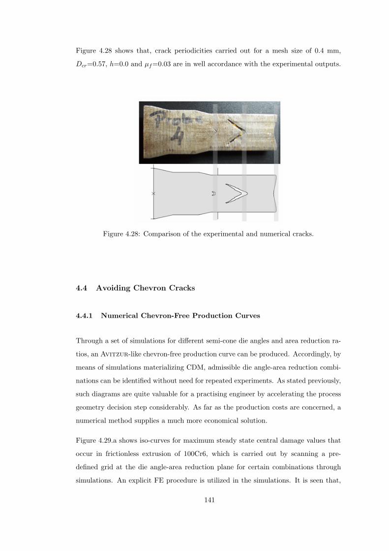
Figure 4.28 shows that, crack periodicities carried out for a mesh size of 0.4 mm,
Dcr=0.57, h=0.0 and µf=0.03 are in well accordance with the experimental outputs.
Figure 4.28: Comparison of the experimental and numerical cracks.
4.4 Avoiding Chevron Cracks
4.4.1 Numerical Chevron-Free Production Curves
Through a set of simulations for different semi-cone die angles and area reduction ra-
tios, an Avitzur-like chevron-free production curve can be produced. Accordingly, by
means of simulations materializing CDM, admissible die angle-area reduction combi-
nations can be identified without need for repeated experiments. As stated previously,
such diagrams are quite valuable for a practising engineer by accelerating the process
geometry decision step considerably. As far as the production costs are concerned, a
numerical method supplies a much more economical solution.
Figure 4.29.a shows iso-curves for maximum steady state central damage values that
occur in frictionless extrusion of 100Cr6, which is carried out by scanning a pre-
defined grid at the die angle-area reduction plane for certain combinations through
simulations. An explicit FE procedure is utilized in the simulations. It is seen that,
141

most desirable conditions with smallest central damage accumulation occur for small
die angles and high area reduction ratios. Critical damage threshold is satisfied for
cases where high reduction ratios meet with high die angles. Figure 4.29.b shows the
scanned grid points on the plane where safe (without crack formation) and unsafe
(with crack formation) simulations are also marked.
Figure 4.29: a) Iso-damage contours for maximum central damage accumulation atsteady-state, b) Simulations with and without cracks, µf=0.
4.4.2 Avoiding Chevrons by Means of Counter Pressure
In this section it is demonstrated that, application of counter pressure introduces a
marked decrease in the central damage accumulation, which in turn increases the
formability of the material through keeping the central tensile triaxiality in tolerable
limits. It is also shown that, for a crack involving process, through systematic increase
of the counter pressure, the crack sizes diminish; where at a certain level of counter
pressure chevron cracks can be completely avoided. Since, in avoiding cracks, the main
motivation is to obtain a hydrostatic compression at the forming zone, for fixed die
geometry and process parameters one could supply additional central compression by
means of employing counter pressure at the extruded nose part of the workpiece. The
142

experimental studies of [191], [192], [193] show that, application of counter pressure
promotes material formability in extrusion by which it becomes possible to extrude
even relatively brittle materials, like MMC of aluminum alloy matrix with SiC par-
ticles, similar to low carbon steels, where the cracks are suppressed. Moreover, it is
demonstrated in these studies that, counter pressure application results in decreased
die exit residual tensile stresses and more homogeneous plastic deformation distribu-
tions at the extrudate where strain gradients are lowered. Besides its advantages,
counter pressure increases the punch force demand of the process and thus has certain
limits governed by the allowable punch and die stresses13.
To the author’s knowledge, there exist no numerical studies on the use of counter pres-
sure to give account for defect-free extrusion. Accordingly, in this follow up section,
the aim is to investigate what (explicit) finite element method suggests on the role of
counter pressure in suppressing crack formations in axi-symmetric forward extrusion.
For this purpose, for single pass reduction of 100Cr6, it is shown that, proper appli-
cation of counter pressure suppresses central crack formation completely, by keeping
the forming zone hydrostatic stress levels in tolerable limits. The deviations of crack
morphologies and sizes with counter pressure application are also examined. Fig-
ure 4.30 shows the employed axi-symmetric model boundary conditions, where for
counter pressure a rather simplistic approach, in which a compressive normal traction
is applied at the workpiece nose with an opposing direction to the punch movement
direction, is pursued. Such an application of the counter pressure in the form of nor-
mal compressive surface pressure deviates from the actual practice where a counter
punch is utilized. However, various trials of the authors show that, simulations in-
volving a counter pressure applied through a counter deformable body increases the
computational time considerably due to additional contact iterations, where, although
the nose deformation pattern may depart at high pressure levels in between two meth-
ods, these differences diminish at distances sufficiently far away from the nose due to
Saint-Venant’s principle.
13 Counter pressure application is also employed as a precision extrusion method, where the under-filling defects are eliminated, [132]. However this type of utilization falls beyond the context of thisstudy.
143

Figure 4.30: Application of the counter pressure.
Starting with, frictionless workpiece-die interface is assumed for a clear demonstration
of the central damage accumulation mechanism. Without any counter pressure, with
the aid of positive triaxial stress state which meets with plastic flow at the forming
zone, a localized damage growth is observed, as demonstrated in Figure 4.31.a, b and c,
which respectively represent the iso-curves for positive hydrostatic stress, equivalent
plastic strain rate and damage rate, one step before the first element deletion, i.e.
occurrence of the first crack. At the die exit, there exists a small amount of surface
deterioration due to residual tensile stresses. At Figure 4.31.d and e, total equivalent
plastic strain and total damage iso-curves are given, respectively. As seen, central
damage rates accumulate to create a continuous damage zone at the central region.
It is not hard to guess that, when this value exceeds the critical threshold, together
with coalescence of micro-voids, macro-crack formations in the form of chevrons take
place.
Figure 4.31: Isomaps for no counter pressure, µf=0.
144

When a counter pressure of 200 MPa is applied to the frictionless simulation, a decrease
is observed in both the intensity and area extent of the central positive hydrostatic
stresses, for the same time increment, as seen in Figure 4.32.a. This amounts for a no-
ticeable decrease in the damage rates, as seen in Figure 4.32.c, where the effectiveness
of the counter pressure application is clearly observed.
Figure 4.32: Isomaps for counter pressure=200 MPa, µf=0.
For the same time step, hydrostatic stress and damage growth distributions for a
certain path defined at the axis of symmetry on the forming zone are respectively
given in Figure 4.33.a and b, for different counter pressure values. Figure 4.33.a shows
that, for a counter pressure of 400 MPa, triaxial stress distribution over the path is
kept compressive through the anticipated stress increase in the central zone in the
compressive direction by means of counter pressure employment. Consequent damage
rates, given in Figure 4.33.b, although show a considerable decrease with increasing
counter pressure, do not boil down to zero for 400 MPa counter pressure. This is
due to the fact that, in the selected mathematical damage model, damage evolution
depends on the sign of each principal stress component but not merely the sign of the
pressure.
145

Figure 4.33: Central line, a) hydrostatic stress, b) damage rate values, for differentcounter pressure levels, µf=0.
In order to further evaluate the effectiveness of intensity of the counter pressure,
analyses for different counter pressure magnitudes, ranging from 0 to 200 MPa, are
conducted for frictionless and frictional conditions. As given in Figure 4.34, for fric-
tionless conditions, it is seen that, a counter pressure of 200 MPa suffices to suppress
crack formation. This finding is analogous to the experimental findings of Wagener
and his colleagues which show the efficiency of the counter pressure in promotion of the
material formability in cold extrusion. It should be noted that, damage accumulation
at the center is not completely bypassed however decreased under the crack threshold,
where the material integrity at the macro-scale is preserved. The experiences of the
author show that, for the selected damage model, the counter pressure values that
should completely withdraw the central damage accumulation should be considerable,
which in turn require unreasonable punch force demands and thus become impracti-
cal. Besides, die and punch stress limitations act as the main obstacles for excessive
amplification of counter pressures. Figure 4.34 also represents the effect of the counter
pressure intensity on crack morphologies. Accordingly, the outputs suggest that, the
crack opening and the crack half width, measured as the arithmetic mean of first three
cracks, show a monotonic decrease with increased counter pressure, which is physically
reasonable, thus anticipated. It is notable that, unlike friction, counter pressure does
not seem to have an effect on the periodicity of the cracks.
146

Figure 4.34: Mean crack dimensions and crack patterns for various counter pressurelevels, µf=0.
For frictionless simulations, the punch force-normalized process time curves are given
in Figure 4.35 for the analyses without counter pressure and with counter pressure of
100 MPa and 200 MPa. Crack involving simulations experience an oscillatory behav-
ior whereas in the simulation without any cracks, no oscillations are observed where
a steady trend is captured in the absence of friction. Moreover, the extent of the
oscillations is strictly dependent on the internal crack size, where in the simulations
with larger cracks, oscillations become more dominant compared to those with smaller
cracks. The anticipated increase in the punch force demand with increasing counter
pressure values reminds one that, in the actual applications, reasonable counter pres-
sure values should be selected for feasibility.
Once a friction of µf=0.04 is applied at die-workpiece interface, crack patterns for
147

Figure 4.35: Punch force demand curves for different counter pressure levels, µf=0.
different counter pressure values take the form demonstrated in Figure 4.36. A re-
markable point is that, in the presence of friction, the counter pressure required for
the crack-free simulations decreases considerably from 200 MPa to 125 MPa. This
is due to the fact that both friction and counter pressure act analogically similar, as
a counter force agent which works in opposite direction with respect to the applied
external pressure of the punch. Another point is that, with the increase of friction,
damage accumulation zones are carried over to the surface rather than center. Thus
under frictional conditions, cracks can be healed with employment of a reduced counter
pressure. The change of the crack sizes as a function of the applied counter pressure
follows a similar trend with the frictionless simulations.
For the frictional conditions, the punch force-normalized process time diagrams are
given in Figure 4.37, for the analyses without counter pressure and with counter
pressure for 75 and 125 MPa, respectively. In accordance with the previous outcomes,
148

Figure 4.36: Mean crack dimensions and crack patterns for various counter pressurelevels, µf=0.04.
the crack size dependent oscillations in the force demand diminish with smaller cracks.
In addition to the counter pressure, the effect of friction also increases the peak load
levels for analyses. Besides, due to friction, the steady trend of the frictionless force
demand curve now experiences a monotonic drop off with the reduction of contacting
surfaces.
Figure 4.38 is to compare the crack morphologies for frictional and frictionless anal-
ysis, at different counter pressure values. The dimensions of the cracks in frictional
simulations come out to be considerably small compared to frictionless simulation
results, which is anticipated.
149

Figure 4.37: Punch force demand curves for different counter pressure levels, µf=0.04.
Figure 4.38: Mean crack dimensions for various counter pressure levels and frictioncoefficients.
As previously shown in Figure 4.33.a and b, employment of counter pressure, although
heals crack occurrence for certain intensities, does not necessarily eliminate the cen-
150

tral damage accumulation completely. Figure 4.39 shows the damage iso-error plots
for certain counter pressure levels in frictionless and frictional simulations. As seen,
for both µf=0, and µf=0.04, once the counter pressure is 100 MPa, discontinuous
chevron crack formations arise. For these cases, damage iso-curves have a discontinu-
ous structure, similar to the crack patterns, where maximum damage values occur at
the crack free-surfaces. The cracks are eliminated for a counter pressure of 200 MPa,
at both of the frictional conditions. It is remarkable that, this time central damage
accumulation has a continuous distribution. Another notable point is that, central
damage intensities in the frictional case are less than those seen in the frictionless
simulation, which is in agreement with the previously stated observations.
Figure 4.39: Damage contours, a) counter pressure=100 MPa, µf=0, b) counter pres-sure=200 MPa, µf=0, c) counter pressure=100 MPa, µf=0.04, d) for counter pres-sure=200 MPa, µf=0.04.
Our final attempt is investigation of the steady state radial damage and equivalent
plastic strain distributions for chevron-free simulations subjected to frictionless and
frictional conditions, as given in Figure 4.40 and 4.41 respectively. Damage plots, given
in Figure 4.40, reveal that, for both frictionless and frictional simulations, counter
pressure decreases damage accumulation in both center and surface considerably. A
comparison of Figure 4.40.a and b shows that, for equal levels of counter pressure,
151

frictional interface conditions result in lower central however higher surface damage
accumulations, compared to the frictionless conditions which is in accordance with
the previous observations.
Figure 4.40: Radial damage distribution for different counter pressure levels (steadystate), a) µf=0, b) µf=0.04.
Coming to Figure 4.41, current employment of counter pressure introduces a difference
in central equivalent plastic strain accumulations for both frictionless and frictional
experiments, where with the increase of applied pressure, central plastic flow is pro-
moted which, although slightly, decreases the overall radial equivalent plastic strain
gradients. This is also in accordance with the experimental findings of Wagener and
his colleagues, where uniform equivalent plastic strain distributions are carried out
with the aid of counter pressure employment. Besides, it is shown that, unlike center,
friction introduces a marked increase in the plastic strain intensities at the surface
region. Accordingly the distribution of equivalent plastic strain has a steeper trend
at the half radial distance closer to the surface.
152
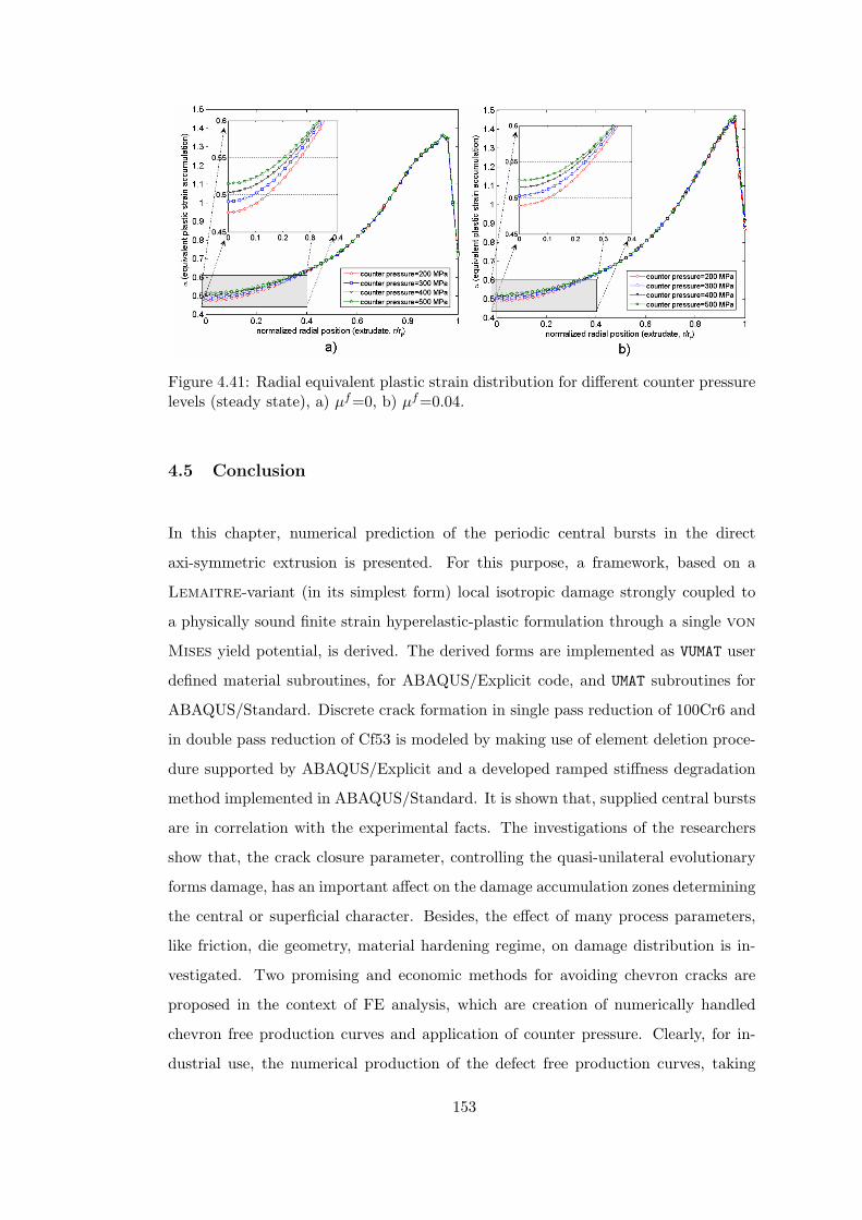
Figure 4.41: Radial equivalent plastic strain distribution for different counter pressurelevels (steady state), a) µf=0, b) µf=0.04.
4.5 Conclusion
In this chapter, numerical prediction of the periodic central bursts in the direct
axi-symmetric extrusion is presented. For this purpose, a framework, based on a
Lemaitre-variant (in its simplest form) local isotropic damage strongly coupled to
a physically sound finite strain hyperelastic-plastic formulation through a single von
Mises yield potential, is derived. The derived forms are implemented as VUMAT user
defined material subroutines, for ABAQUS/Explicit code, and UMAT subroutines for
ABAQUS/Standard. Discrete crack formation in single pass reduction of 100Cr6 and
in double pass reduction of Cf53 is modeled by making use of element deletion proce-
dure supported by ABAQUS/Explicit and a developed ramped stiffness degradation
method implemented in ABAQUS/Standard. It is shown that, supplied central bursts
are in correlation with the experimental facts. The investigations of the researchers
show that, the crack closure parameter, controlling the quasi-unilateral evolutionary
forms damage, has an important affect on the damage accumulation zones determining
the central or superficial character. Besides, the effect of many process parameters,
like friction, die geometry, material hardening regime, on damage distribution is in-
vestigated. Two promising and economic methods for avoiding chevron cracks are
proposed in the context of FE analysis, which are creation of numerically handled
chevron free production curves and application of counter pressure. Clearly, for in-
dustrial use, the numerical production of the defect free production curves, taking
153

the change of many previously mentioned process parameters into account, is pos-
sible. It is shown that, chevron crack formations can be prevented at the expense
of increased load demand, not mentioning the mechanism complications, by devising
counter pressure, which helps keeping the tensile triaxial stress fields under tolerable
limits. Further micro-mechanical and experimental research should be conducted for
proper determination of the material parameters of the actual material together with
more advanced damage rate forms.
154

CHAPTER 5
CLOSURE and FUTURE PERSPECTIVES
5.1 Closure
An extensive theoretical and numerical study on modeling isotropic ductile damage for
finite strain plasticity is presented. For this purpose a framework for damage coupled
hyperelastic-(visco)plasticity is presented in principal axes in an Euclidean setting
in a local basis. The unified functional framework for the governing functions of plas-
ticity and damage does not assume particular restrictions on the forms. This gives
rise to implementation of a broad range of damage and plasticity models, strongly
coupled through a single yield surface. It is shown that, principal axes formulation
provides convenience in active-passive damage evolutionary conditions which depends
on eigen-projections besides finite hyperelastic-plastic framework, reducing tensorial
differentials to simple differentials with respect to scalars. Inclusion of thermal effects
is also presented. Unilateral damage evolutionary forms are given with special em-
phasis on the practicality and efficiency of formulations in principal axes. Moreover
local integration procedures are summarized starting from a full equation set which
are simplified step by step initially to two and finally to one. Also different operator
split methodologies such as elastic predictor-damage plastic corrector (simultaneous
plastic-damage solution scheme) and elastic predictor-plastic corrector-damage dete-
riorator (staggered plastic-damage solution scheme) are given. To this end regarding
consistent material moduli are derived. The models are implemented as user defined
material subroutines for ABAQUS and MSC.Marc. The efficiency and the predictive
performances of the models are studied with a set of sample problems.
155

5.2 Future Perspectives
Following topics constitute current and future research interests,
• Extension of the thermo-mechanical setting to include material anisotropy, where
damage induced anisotropic behavior together with hyperelastic and plastic
anisotropies will also be developed.
• Investigations on additional damage models, which are micro-mechanically based.
• Nonlocal material modelling with special emphasis of the ellipticity and hyper-
bolicity loss in the IBVPs of quasi static and dynamic frameworks, respectively.
Besides, investigation of localization limiting properties of the integral and gra-
dient localizers.
• Evaluation of local integration algorithms together with efficiency and accuracy
observations.
• Use of adaptive mesh refinement methods with consistent error measures for
crack propagation.
• Extension of the explicit adiabatic framework to cope with impact and projectile
penetration problems.
• Material parameter identification through inverse methods.
156

REFERENCES
[1] ABAQUS User Subroutines Reference Manual - ABAQUS Version 6.6, [2006]:ABAQUS, Inc.
[2] Abu Al-Rub, R. K.; Voyiadjis, G. Z. [2003]: “On the coupling of anisotropicdamage and plasticity models for ductile materials”, International Journal ofSolids and Structures, Vol. 40, 2611–2643.
[3] Anand, L. [1979]: “On Hencky’s Approximate Strain-Energy Function for Mod-erate Deformations”, ASME Journal of Applied Mechanics, Vol. 46, 78–82.
[4] Anand, L. [1986]: “Moderate Deformations in Extension-Torsion of Incom-pressible Isotropic Elastic Materials”, Journal of the Mechanics and Physics ofSolids, Vol. 34, 293–304.
[5] Andrade Pires, F. M.; de Souza Neto, E. A.; Owen, D. R. J. [2004]:“On the finite element prediction of damage growth and fracture initiation infinitely deforming ductile materials”, Computer Methods in Applied Mechanicsand Engineering , Vol. 193, 5223–5256.
[6] Aravas, N. [1986]: “The analysis of void growth that leads to central burstsduring extrusion”, Journal of Engineering for Ind , Vol. 34, 55–79.
[7] Areias, P. M. A.; Cesar de Sa, J. M. A.; Conceicao Antonio, C. A.[2003]: “A gradient model for finite strain elastoplasticity coupled with damage”,Finite Elements in Analysis and Design, Vol. 39, 1191–1235.
[8] Argyris, J. H.; Doltsinis, J. St. [1981]: “On the natural formulation andanalysis of large deformation coupled thermomechanical problems”, ComputerMethods in Applied Mechanics and Engineering , Vol. 25, 195–253.
[9] Armero, F.; Simo, J. C. [1993]: “A new unconditionally stable fractionalstep method for non-linear coupled thermomechanical problems”, InternationalJournal for Numerical Methods in Engineering , Vol. 35, 737–766.
[10] Armero, F.; Simo, J. C. [1993]: “A priori stability estimates and uncondition-ally stable product formula algorithms for nonlinear coupled thermoplasticity”,International Journal of Plasticity , Vol. 9, 749–782.
[11] Asaro, R. J. [1983]: “Micromechanics of crystals and polycrystals. Advancesin Applied Mechanics, Vol. 23, 1–115.
[12] Auricchio, F.; Taylor, R. L. [1999]: “A return-map algorithm of generalassociative isotropic elastoplastic materials in large deformation regimes”, In-ternational Journal of Plasticity , Vol. 15, 1359–1378.
157

[13] Avitzur, B. [1968]: “Analysis of central bursting defects in extrusion and wiredrawing”, Journal of Mechanics and Physics of Solids, Vol. 90, 79–91.
[14] Baker, G.; de Borst, R. [2005]: “An anisotropic thermomechanical damagemodel for concrete at transient elevated temperatures”, Philosophical Transac-tions of the Royal Society A, Vol. 363, 2603–2628.
[15] Bakhshi-Jooybari, M. [2002]: “A theroretical and experimental study of fric-tion in metal forming by the use of the forward extrusion process”, Journal ofMaterials Processing Technology , Vol. 125-126, 369–374.
[16] Basaran, C.; Nie, S. [2004]: “An irreversible thermodynamics theory fordamage mechanics of solids”, Intertational Journal of Damage Mechanics, Vol.13, 205–223.
[17] Bazant, Z. [2000]: “Structural stability”, International Journal of Solids andStructures, Vol. 37, 55–67.
[18] Bellenger, E.; Bussy, P. [1998]: “Plastic and viscoplastic damage modelswith numerical treatment for metal forming processes”, Journal of MaterialsProcessing Technology , Vol. 80-81, 591–596.
[19] Berski, S.; Dyja, H.; Banaszek, G.; Janik, M. [2004]: “Theoretical anal-ysis of bimetallic rods extrusion process in double reduction die”, Journal ofMaterials Processing Technology , Vol. 153-154, 583–588.
[20] Bielski, J.; Skrzypek, J. J.; Kuna-Ciskal, H. [2006]: “Implementation ofa model of coupled elastic-plastic unilateral damage material to finite elementcode”, International Journal of Damage Mechanics, Vol. 15, 5–39.
[21] Bigoni, D.; Zaccaria, D. [1994]: “Eigenvalues of the elastoplastic constitutiveoperator”, Z. angew. Math. Mech., Vol. 74, No. 8, 355–357.
[22] Bonnet, J.; Wood, R.[1997]: Nonlinear Continuum Mechanics for FiniteElement Analysis, Cambridge University Press.
[23] Bonora, N. [1997]: “A nonlinear CDM model for ductile failure”, EngineeringFracture Mechanics, Vol. 58, 11–28.
[24] Bonora N.; Gentile D.; Pirondi A.; Newaz G. [2005]: “Ductile damageevolution under triaxial state of stress: theory and experiments”, InternationalJournal of Plasticity , Vol. 21(5), 981–1007.
[25] Bonora N.; Ruggiero A.; Esposito L.; Gentile D. [2006]: “CDM mod-eling of ductile failure in ferritic steels: Assessment of the geometry transfer-ability of model parameters”, International Journal of Plasticity , Vol. 22(11),2015–2047.
[26] Borja, R. I.; Sama, K. M.; Sanz, P. F. [2003]: “On the numerical integra-tion of three-invariant elastoplastic constitutive models”, Computer Methods inApplied Mechanics and Engineering , Vol. 192, 1227–1258.
[27] Borouchaki, H.; Laug, P.; Cherouat, A.; Saanouni, K. [2005]: “Adap-tive remeshing in large plastic strain with damage”, International Journal forNumerical Methods in Engineering , Vol. 63, 1–36.
158

[28] Børvik, T.; Hopperstad, O. S.; Berstad, T.; Langseth, M. [2001]: “Nu-merical solution of plugging failure in balistic penetration”, International Jour-nal of Solids and Structures, Vol. 38, 6241–6264.
[29] Børvik, T.; Hopperstad, O. S.; Berstad, T.; Langseth, M. [2002]: “Per-foration of 12mm thick steel plates by 20mm diameter projectiles with flat,hemispherical and conical noses Part II: numerical simulations”, InternationalJournal of Impact Engineering , Vol. 27, 37–64.
[30] Brozzo, P.; Deluca, B.; Rendina, R. [1972]: “A new method for the pre-diction of formability limits in metal sheets, sheet metal forming and formabil-ity”, Proceedings of the Seventh Biannual Conference of the International DeepDrawing Research Group.
[31] Brunig, M. [2003]: “An anisotropic ductile damage model based on irreversiblethermodynamics”, International Journal of Plasticity , Vol. 19, 1679–1713.
[32] Brunig, M.; Ricci, S. [2005]: “Nonlocal continuum theory of anisotropicallydamaged metals. International Journal of Plasticity , Vol. 21, 1346–1382.
[33] Camacho, A. M.; Gonzales, C.; Rubio, E. M.; Sebastian, M. A. [2006]:“Influence of geometrical conditions on central burst appearance in axisymmetricdrawing procsses”, Journal of Materials Processing Technology , Vol. 177, 304–306.
[34] Canadija, M.; Brnic, J. [2004]: “Associative coupled thermoplasticity atfinite strain with temperature-dependent material parameters”, InternationalJournal of Plasticity , Vol. 20, 1851–1874.
[35] Cervera, M.; Chiumenti, M.; de Saracibar, A. C. [2004]: “Shear bandlocalization via local J2 continuum damage mechanics”, Computer Methods inApplied Mechanics and Engineering , Vol. 193, 849–880.
[36] Ceretti, E.; Taupin, E.; Altan, T. [1997]: “Simulation of metal flow andfracture applications in orthogonal cutting, blanking, and cold extrusion”, An-nals of the CIRP , Vol. 46, 187–190.
[37] Cesar de Sa, J. M. A.; Areias, P. M. A.; Zheng, C. [2006]: “Damage mod-elling in metal forming problems using an implicit non-local gradient model”,Computer Methods in Applied Mechanics and Engineering , Vol. 195, 6646–6660.
[38] Chaboche, J. L. [2003]: Chapter 2.04, Damage Mechanics. In: ComprehensiveStructural Integrity. Elsevier Ltd., 213–284.
[39] Chandrakanth, S.; Pandey, P. C. [1993]: “A new ductile damage evolutionmodel”, International Journal of Fracture, Vol. 60, R73–R76.
[40] Chandrakanth, S.; Pandey, P. C. [1995]: “An exponential ductile con-tinuum damage model for metals”, International Journal of Fracture, Vol. 72,293–310.
[41] Chen, C. C.; Oh, S. I.; Kobayashi, S. [1979]: “Ductile fracture in axisym-metric extrusion and drawing”, J. Eng. Ind., Vol. 101, 13–35.
159

[42] Chen, D.; Syu, S.; Wu, C.; Lin S. [2007]: “Investigation into cold extrusionof aliminum billets using three-dimensional finite element method”, Journal ofMaterials Processing Technology , Vol. 192-193, 188–193.
[43] Cherouat, A.; Saanouni, K.; Hammi, Y. [2002]: “Numerical improvement ofthin tubes hydroforming with respect to ductile damage”, International Journalof Mechanical Sciences, Vol. 44, 2427–2446.
[44] Cherouat, A.; Saanouni, K.; Hammi, Y. [2003]: “Improvement of forgingprocess of a 3D complex part with respect to damage occurence”, Journal ofMaterials Processing Technology , Vol. 142, 307–317.
[45] Chorin, A. J.; Hughes, T. J. R.; McCracken, M. F.; Marsden, J. E.[1978]: “Product formulas and numerical algorithms”, Communications on Pureand Applied Mathematics, Vol. XXXI, 205–256.
[46] Cockroft, M. G.; Latham, D. J. [1968]: “Ductility and the workability ofmetals”, Journal of the Institute of Metals Vol. 96, 33–39.
[47] Coleman, B.; Gurtin, M.[1967]: “Thermodynamics of internal state vari-ables”, The J. Chemical Physics, Vol. 47, 597–613.
[48] da Cunda, L. A. B.; Bittencourt, E.; Creus, G. [1998]: “Analysis ofductile damage coupled with thermoplasticity by the FEM”, In: Idelsohn, S.;Onate, E.; Dvorkin, E. (Eds.), Computational Mechanics New Trends andApplications, CIMNE, Barcelona, Spain, 1–13.
[49] Dhar, S.; Sethuraman, R.; Dixit, P. [1996]: “A continuum damage me-chanics model for void growth and micro-crack initiation”, Engineering FractureMechanics, Vol. 53, 917–928.
[50] Doghri, I. [2000]: Mechanics of Deformable Solids, Linear and Nonlinear,Analytical and Computational Aspects, Springer-Verlag, Berlin Heidelberg.
[51] Drabek, T.; Bohm, H. J. [2005]: “Damage models for studying ductile matrixfailure in composites”, Computational Materials Science, Vol. 32, 329–336.
[52] Elgueta, M.; Cortes, C. [1999]: “Application of continuum damage theoryin metalforming processes”, Journal of Materials Processing Technology , Vol.95, 122–127.
[53] Ekh, M.; Lillbacka, R.; Runesson, K. [2004]: “A model framework foranisotropic damage coupled to crystal (visco)plasticity”, International Journalof Plasticity , Vol. 20, 2143–2159.
[54] Ekh, M.; Menzel, A. [2006]: “ Efficient iteration schemes for anisotropichyperelasto-plasticity”, International Journal for Numerical Methods in Engi-neering, Vol. 66, 707–721.
[55] Enakoutsa, K.; Leblond, J. B.; Perrin, G. [2007]: “Numerical implemen-tation and assessment of a phenomenological nonlocal model of ductile rupture”,Computer Methods in Applied Mechanics and Engineering , Vol. 196, 1946–1957.
[56] Engelen, R. A. B. [2005]: Plasticity induced damage in metals, PhD thesis,Technische Universiteit Eindhoven
160

[57] Eterovic, A. L.; Bathe, K., J. [1990]: “A hyperelastic-based large strainelasto-plastic constitutive formulation with combined isotropic-kinematic hard-ening using the logarithmic stress and strain measures”, International Journalof Numerical Methods in Engineering , Vol. 30, 1099–1114.
[58] Freudenthal, A. M. [1950]: The Inelastic Behavior in Solids, Wiley, NewYork.
[59] Ganapathysubramanian, S.; Zabaras, N. [2003]: “Computational designof deformation processes for materials with ductile damage”, Computer Methodsin Applied Mechanics and Engineering , Vol. 192, 147–183.
[60] Ganczarski, A. [2003]: “Chapter 10. Thermo-Damage Coupling Modellingand Applications for Creep Conditions”, In: Skrzypek, J. J; Ganczarski,A. W. (Eds.), Anisotropic Behavior of Damaged Materials, Springer-VerlagBerlin Heidelberg, 317–349.
[61] Gelin, J. C. [1998]: “Modelling of damage in metal forming simulations”,Journal of Materials Processing Technology , Vol. 80–81, 24–32.
[62] Giardini C.; Ceretti, E.; Maccarini, G. [1995]: “Formability in extru-sion forging: the influence of die geometry and friction conditions”, Journal ofMaterials Processing Technology , Vol. 54, 302–308.
[63] Goijaerts, A. M.; Govaert, L. E.; Baaijens, F. P. T. [2001]: “Evaluationof ductile fracture models for different metals in blanking”, J. Mater. Process.Technol., Vol. 110, 312–323.
[64] Gologanu, M.; Leblond, J.-B.; Perrin, G.; Devaux, J. [1997]: “Trans-verse ductility of metal matrix composites”, In: Suquet, P. (Eds.), ContinuumMicromechanics, CISM Lecture Series, Springer, 61–130.
[65] Gunawardena, S. R.; Jansson, S.; Leckie, F. A. [1991]: “Transverse duc-tility of metal matrix composites”, In: Haritos, K.; Newaz, K.; Mall, S.(Eds.), Failure Mechanisms in High Temperature Composite Naterials, ASME,New York, NY, 23–30.
[66] Guo, Y. B.; Yen, D. W. [2004]: “A FEM study on mechanisms of discon-tinuous chip formation in hard machining”, Journal of Materials ProcessingTechnology , Vol. 155–156, 1350–1356.
[67] Guo, Y. B.; Yen, D. W.; Woodbury, K. A. [2004]: “Dynamic materialbehavior modeling using internal state variable plasticity and its applications inhard machining”, Journal of Manufacturing Science and Engineering , Vol. 128,749–759.
[68] Gurson, A. L. [1977]: “Continuum theorie of ductile rupture by void nucleationand growth: Part I. Yield criteria and flow rules for porous ductile media”, J.Eng. Mater. Technol. Trans. ASME , Vol. 99, 2–15.
[69] Hakansson, P.; Wallin, M.; Ristinmaa, M.[2005]: “Comparison ofisotropic hardening and kinematic hardening in thermoplasticity”, InternationalJournal of Plasticity, Vol. 21, 1435–1460.
161

[70)] Hakansson, P.; Wallin, M.; Ristinmaa, M.[2006]: “Thermomechanicalresponse of non-local porous material”, International Journal of Plasticity, Vol.22, 2066–2090.
[71] Hambli, R.; Potiron, A. [2000]: “Finite element modelling of sheet-metalblanking operations with experimental verification”, Journal of Materials Pro-cessing Technology , Vol. 102, 257–265.
[72] Hambli, R.; Badie-Levet, D. [2000]: “Damage and fracture simulation dur-ing the extrusion process”, Computer Methods in Applied Mechanics and Engi-neering , Vol. 186, 109–120.
[73] Hambli, R. [2001]: “Comparison between Lemaitre and Gurson damage modelsin crack growth simulation during blanking process”, International Journal ofMechanical Sciences, Vol. 43, 2769–2790.
[74] Hancock, J. W.; Mackenzie, A. C. [1950]: “On the mechanisms of ductilefracture in high-strength steels subjected to multi-axial stress states”, Journalof Mechanics and Physics of Solids, Vol. 24, 147–169.
[75)] Hansen, N. R.; Schreyer, H. L. [1994]: “A thermodynamically consistentframework for theories of elastoplasticity coupled with damage”, InternationalJournal of Solids and Structures, Vol. 31, 359–389.
[76] Hill, R. [1950]: The Mathematical Theory of Plasticity , Oxford UniversityPress, London.
[77] Hughes, T. J. R. [1983]: “Analysis of transient algorithms with particular ref-erence to stability behavior”, In: Belytschko, T.; Hughes, T. J. R. (Eds.),Computational Methods for Transient Analysis, North-Holland, 67–155.
[78] Hughes, T. J. R. [2000]: The Finite Element Method–Linear Static and Dy-namic Finite Element Analysis, Dover Publishers, New York.
[79] Ibrahimbegovic, A. [1994]: “Equivalent spatial and material descriptions offinite deformation elastoplasticity in principal axes”, International Journal ofSolids and Structures, Vol. 31, 3027–3040.
[80] Ibrahimbegovic, A.; Gharzeddine, F. [1999]: “Finite deformation plasticityin principal axes: from a manifold to the Euclidean setting”, Computer Methodsin Applied Mechanics and Engineering , Vol. 171, 341–369.
[81] Ibrahimbegovic, A.; Chorfi, L. [2000]: “Viscoplasticity model at finite de-formations with combined isotropic and kinematic hardening”, Computers andStructures, Vol. 77, 509–525.
[82] Jennison, H. C. [1930]: “Certain types of defects in copper wire caused byimproper dies and drawing practice”, Proc. Inst. Metal Div. AIME , Vol. 89.
[83] Jirasek, M.; Bazant, Z. [2001]: Inelastic Analysis of Structures, John Wileyand Sons, England.
[84] Johnson, G. R.; Cook, H. W [1985]: “Fracture Characteristics of ThreeMetals Subjected to Various Strains, Strain Rates, Temperature and Pressures”,Engineering Fracture Mechanics, Vol. 21(1), 31–48.
162

[85] Ju, J. W. [1989a]: “Energy-based coupled elastoplastic damage models at finitestrains”, Journal of Engineering Mechanics, Vol. 115, 2507–2525.
[86] Ju, J. W. [1989b]: “On energy-based coupled elastoplastic damage theories:constitutive modelling and computational aspects”, International Journal forSolids and Structures, Vol. 25, 803–833.
[87] Ju, J. W. [1990]: “Isotropic and anisotropic damage variables in continuumdamage mechanics”, Journal of Engineering Mechanics, Vol. 116, 283–287.
[88] Kachanov, L. M. [1958]: “Time of the rupture process under creep condi-tions”, Izv. Akad. Nauk. SSR, Vol. 8, 26–31.
[89] Ko, D.; Kim, B. [2000]: “The prediction of central burst defects in extrusionand wire drawing”, Journal of Materials Processing Technology , Vol. 102, 19–24.
[90] Komori, K. [1999]: “Simulation of chevron crack formation and evolution indrawing”, International Journal of Mechanical Sciences, Vol. 41, 1499–1513.
[91] Komori, K. [2003]: “Effect of ductile fracture criteria on chevron crack forma-tion and evolution in drawing”, International Journal of Mechanical Sciences,Vol. 45, 141–160.
[92] Krajcinovic, D. [1996]: Damage Mechanics, Elsevier, Amsterdam.
[93] Krieg, R. D.; Krieg, D. B. [1977]: “Accuracies of numerical solution methodsfor the elastic-perfectly plastic model”, J. Pressure Vessel Tech., A.S.M.E., Vol.99, 510–515.
[94] Lee, E. H. [1969]: “Elasto-plastic deformation at finite strains”, ASME Journalof Applied Mechanics, Vol. 36, 1–6.
[95] Lemaitre, J. [1971]: Evaluation of dissipation and damage in metals. In: Pro-ceedings of I.C.M. 1, Kyoto, Japan.
[96] Lemaitre, J. [1985]: “A continuous damage mechanics model for ductilefracture”, Journal of Engineering Materials and Technology, Transactions ofASME , Vol. 107, 83–89.
[97] Lemaitre, J.; Chaboche, J. [1990]: Mechanics of Solid Materials, CambridgeUniversity Press, Cambridge.
[98] Lemaitre, J. [1996]: A Course on Damage Mechanics, Springer-Verlag, Berlin.
[99] Lemaitre, J.; Desmorat, R. [2005]: Engineering Damage Mechanics,Springer-Verlag, Berlin Heidelberg.
[100] Lestriez, P.; Saanouni, K.; Mariage, J. F.; Cherouat, A. [2004]: “Nu-merical prediction of ductile damage in metal forming proceses including thermaleffects”, International Journal of Damage Mechanics, Vol. 13, 59–80.
[101] Lim, L. G.; Dunne, F. P. E. [1997]: “Modelling central bursting in the extru-sion of particulate reinforced metal matrix composite materials”, Int. J. Mach.Tools Manufact., Vol. 37, 901–915.
163

[102] Lin R. C.; Brocks W.; Betten J. [2006]: “On internal dissipation inequali-ties and finite strain inelastic constitutive laws: Theoretical and numerical com-parisons”, International Journal of Plasticity , Vol. 22, 1825–1857.
[103] Lin, J.; Liu, Y.; Dean, T. A. [2005]: “A review on damage mechanisms,models and calibration methods under various deformation conditions”, Inter-national Journal of Damage Mechanics, Vol. 14, 299–319.
[104] Lubarda, V. A.; Krajcinovic, D.; Mastilovic, S. [1994]: “Damage modelfor brittle elastic solids with unequal tensile and compressive strength”, Engi-neering Fracture Mechanics, Vol. 49, 681–697.
[105] Lubliner, J. [1984]: “A maximum-dissipation principle in generalized plastic-ity”, Acta Mechanica, Vol. 52, 225–237.
[106] Lubliner, J. [1990]: Plasticity Theory , Macmillan Publishing Company, NewYork.
[107] Lammer, H.; Tsakmakis, Ch. [2000]: “Discussion of coupled elastoplasticityand damage constitutive equations for small and finite deformations”, Interna-tional Journal of Plasticity , Vol. 16, 495–523.
[108] Mackerle, J. [2006]: “Finite element modelling and simulation of bulk mate-rial forming”, International Journal for Computer-Aided Engineering and Soft-ware, Vol. 23, 250–342.
[109] Marsden, J. E.; Hughes, T. J. R. [1994]: Mathematical Foundations ofElasticity , Dover, New York.
[110] Mathews, J. H.; Fink, K. D. [1999]: Numerical Methods Using MATLAB ,Prentice Hall, Upper Saddle River, NJ.
[111] Maugin, G. A. [1992]: The Thermomechanics of Plasticity and Fracture, Cam-bridge University Press, Cambridge.
[112] McAllen, P. J.; Phelan, P. [2005]: “Ductile fracture by central bursts indrawn 2011 aliminium wire”, International Journal of Fracture, Vol. 135, 19–33.
[113] McAllen, P. J.; Phelan, P. [2007]: “Numerical analysis of axisymmetric wiredrawing by means of a coupled damage model”, Journal of Materials ProcessingTechnology , Vol. 183, 210–218.
[114] McVeigh, C.; Liu, W. K. [2006]: “Prediction of central bursting during ax-isymmetric cold extrusion of a metal alloy containing particles”, InternationalJournal of Solids and Structures, Vol. 43, 3087–3105.
[115] Mediavilla, J. [2005]: Continuous and discontinuous modelling of ductile frac-ture, PhD thesis, Technische Universiteit Eindhoven.
[116)] Mediavilla, J.; Peerlings, R. H. J.; Geers, M. G. D. [2006]: “A non-local triaxiality-dependent ductile damage model for finite strain plasticity”,Computer Methods in Applied Mechanics and Engineering , Vol. 195, 4617–4634.
164

[117] Menzel, A.; Steinmann, P. [2001]: “A theoretical and computational frame-work for anisotropic continuum damage mechanics at large strains”, Interna-tional Journal of Solids and Structures, Vol. 38, 9505–9523.
[118] Menzel, A.; Ekh, M.; Runesson, K.; Steinmann, P. [2005]: “A frame-work for multiplicative elastoplasticity with kinematic hardening coupled toanisotropic damage”, International Journal of Plasticity , Vol. 21, 397–434.
[119] Miehe, Ch. [1994]: “Aspects of the formulation and finite element implemen-tation of large strain isotropic elasticity”, International Journal for NumericalMethods in Engineering , Vol. 37, 1981–2004.
[120] Miehe, Ch. [1996]: “Numerical application of algorithmic (consistent) tangentmoduli in large-strain computational inelasticity”, Computer Methods in AppliedMechanics and Engineering , Vol. 134, 223–240.
[121] Miehe, Ch. [1998]: “Comparison of two algorithms for the computation offourth-order isotropic tensor functions”, Computers and Structures, Vol. 66,37–43.
[122] Moritoki, H.; Okuyama, E. [1998]: “Prediction of central bursting in extru-sion”, Journal of Materials Processing Technology , Vol. 80-81, 579–584.
[123] Mousavi, S. A. A. A.; Feizi, H.; Madoliat, R. [2007]: “Investigations onthe effects of ultrasonic vibrations in extrusion process”, Journal of MaterialsProcessing Technology , Vol. 187-188, 657–661.
[124] MSC.Marc Volume A: Theory and User Information, [2006]: MSC.Software Cor-poration.
[125] MSC.Marc Volume D: User Subroutines and Special Routines, [2006]:MSC.Software Corporation.
[126] Nahshon, K.; Hutchinson, J. W. [2008]: “Modification of the Gurson Modelfor shear failure ”, European Journal of Mechanics - A/Solids, Vol. 27, 1–17.
[127] Needleman, A. [1988]: “Material rate dependence and mesh sensitivity in lo-calization problems”, Computer Methods in Applied Mechanics and Engineering ,Vol. 67, 69–85.
[128] Nesnas, K.; Saanouni, K. [2002]: “Integral formulation of coupled damageand viscoplastic constitutive equations”, International Journal of Damage Me-chanics, Vol. 11, 367–397.
[129] Norasethasopon, S.; Yoshida, K. [2008]: “Prediction of chevron crack ini-tiation in inclusion copper shaped-wire drawing”, Engineering Failure Analysis,Vol. 15, 378–393.
[130] Ogden, R. W. [1984]: Non-Linear Elastic Deformations, Ellis Horwood Lim-ited, Chichester.
[131] Ortiz, A.; Popov, E. P. [1985]: “Accuracy and stability of integration al-gorithms for elastoplastic constitutive relations”, International Journal for Nu-merical Methods in Engineering, Vol. 21, 1561–1576.
165

[132] Osakada, K.; Matsumoto, R.; Otsu, M.; Hanami, S. [2005]: “Precisionextrusion methods with double axis servo-press using counter pressure”, Annalsof the CIRP, Vol. 1, 245–248.
[133] Ottosen, N. S.; Ristinmaa, M. [2005]: The Mechanics of Constitutive Mod-elling , Elsevier.
[134] Ottosen, N., S.; Runesson, K. [1991]: “Acceleration waves in elasto-plasticity”, International Journal of Solids and Structures, Vol. 28, No. 2, 135–159.
[135] Oyane, M. [1972]: “Criteria of ductile fracture strain”, Bulletin of JSME , Vol.15, 1507–1513.
[136] Oyane, M.; Sato, T.; Okimoto, K.; Shima, S. [1979]: “Criteria for ductilefracture and their applications”, J. Mech. Work. Technol., Vol. 4, 65–81.
[137] Peng, X.; Qin, Y.; Balendra, R. [2003]: “FE analysis of springback andsecondary yielding effect during forward extrusion”, Journal of Materials Pro-cessing Technology , Vol. 135, 211–218.
[138] Pe rez-Foguet, A.; Rodrıguez-Ferran, A.; Huerta, A. [2000]: “Nu-merical differentiation for local and global tangent operators in computationalplasticity”, Computer Methods in Applied Mechanics and Engineering , Vol. 189,277–296.
[139] Perzyna, P. [1968]: “Fundamental problems in viscoplasticity”, Advances inApplied Mechanics, Vol. 9, 243–322.
[140] Perzyna, P. [1990]: “Constitutive equations of dynamic plasticity”, In:Kleiber, M.; Konig, J.A. (Eds.), Inelastic Solids and Structures, AntoniSawczuk Memorial Volume, Pineridge Press, Swansea, UK, pp. 111–129.
[141] Pirondi, A.; Bonora, N.; Steglich, D.; Brocks W.; Hellmann, D.[2006]: “Simulation of failure under cyclic plastic loading by damage models”,International Journal of Plasticity , Vol. 22(11), 2146–2170.
[142] Plancak, M. [1990]: “Stress distribution within the specimen in cold forwardextrusion of steel”, Journal of Materials Processing Technology , Vol. 24, 387–394.
[143] Prot, V.; Skallerud, B.; Holzapfel, G. A. [2007]: “Transversely isotropicmembrane shells with application to mitral valve mechanics. Constitutive mod-elling and finite element implementation”, International Journal for NumericalMethods in Engineering , (in press).
[144] Rabotnov, Y. [1968]: “Creep rupture”, In: Hetenyi, M.; Vincenti, W.(Eds.), Applied Mechanics. Proceedings of the 12th International Congress ofApplied Mechanics, Springer-Verlag, Berlin, 342–320.
[145] Ragab, A. R.; Samy, S. N.; Saleh, Ch. A. R. [2005]: “Prediction of centralbursting in drawing and extrusion of voided metals”, J. Manufacturing Scienceand Engineering, ASME , Vol. 127, 698–702.
166

[146] Rajak, S. A.; Reddy, N. V. [2005]: “Prediction of internal defects in planestrain rolling”, Journal of Materials Processing Technology , Vol. 159, 409–417.
[147] Reckwerth, D.; Tsakmakis, Ch. [2003]: “The principle of generalized energyequivalence in the continuum damage mechanics”, In: Hutter, K.; Baaser,H., Eds. Deformation and Failure in Metallic Materials, Springer-Verlag BerlinHeidelberg, 381–406.
[148] Reese, S.; Wriggers, P. [1997]: “A material model for rubber-like polymersexhibiting plastic deformation: computational aspects and a comparison withexperimental results”, Computer Methods in Applied Mechanics and Engineer-ing , Vol. 148, 279–298.
[149] Rice, J. R.; Tracey, D. M. [1969]: “On the ductile enlargement of voidsin triaxial stress fields”, Journal of Mechanics and Physics of Solids, Vol. 17,201–217.
[150] Rojek, J.; Zienkiewicz, O. C.; Onate, E.; Postek, E. [2001]: “Advancesin FE explicit formulation for simulation of metalforming processes”, Journal ofMaterials Processing Technology , Vol. 119, 41–47.
[151] Rojek, J.; Onate, E.; Postek, E. [1998]: “Application of explicit FE codesto simulation of sheet and bulk metal forming processes”, Journal of MaterialsProcessing Technology , Vol. 80-81, 620–627.
[152] Rousselier, G. [1987]: “Ductile fracture models and their potential in localapproach of fracture”, Nucl. Eng. Design, Vol. 105, 97–111.
[153] Saanouni, K.; Hammi, Y. [2000]: “Numerical simulation of damage in metalforming processes”, In: Benallal, A. (Eds.), Continuous Damage and Frac-ture, Elsevier, Amsterdam, 353–363.
[154] Saanouni, K.; Chaboche, J. L. [2003]: Chapter 3.06, Computational Dam-age Mechanics: Application to Metal Forming Simulation. In: ComprehensiveStructural Integrity. Elsevier Ltd., 319–374.
[155] Saanouni, K.; Mariage, J. F.; Cherouat, A.; Lestriez, P. [2004]: “Nu-merical prediction of discontinuous central bursting in axisymmetric forwardextrusion by continuum damage mechanics”, Computers and Structures, Vol.82, 2309–2332.
[156] Saleh, Ch. A. R.; Ragab, A. R.; Samy, S. N. [2005]: “Prediction of voidgrowth in drawing and extrusion of voided metals”, Mechanics of Materials,Vol. 37, 915–924.
[157] Shabaik, A. H. [1991]: “Mechanics of plastic deformation in metal forming pro-cesses: Experimental and numerical methods”, Journal of Materials ProcessingTechnology , Vol. 27, 3–24.
[158] Simo, J. C. [1988a]: “A framework for finite strain elastoplasticity based ona maximum plastic dissipation and the multiplicative decomposition. Part I:Continuum Formulation”, Computer Methods in Applied Mechanics and Engi-neering , Vol. 66, 199–219.
167

[159] Simo, J. C. [1988b]: “A framework for finite strain elastoplasticity based ona maximum plastic dissipation and the multiplicative decomposition. Part II:Computational aspects”, Computer Methods in Applied Mechanics and Engi-neering , Vol. 68, 1–31.
[160] Simo, J. C.; Govindjee, S. [1991]: “Non-linear B-stability and symmetrypreserving return mapping algorithms for plasticity and viscoplasticity”, Inter-national Journal for Numerical Methods in Engineering, Vol. 31, 151–176.
[161] Simo, J. C. [1992]: “Algorithms for multiplicative plasticity that preserve theform of the return mappings of the infinitesimal theory”, Computer Methods inApplied Mechanics and Engineering , Vol. 99, 61–112.
[162] Simo, J. C.; Miehe, Ch. [1992]: “Associative coupled thermoplasticity atfinite strains: Formulation, numerical analysis and implementation”, ComputerMethods in Applied Mechanics and Engineering, Vol. 98, 41–104.
[163] Simo, J. C. [1994]: “Topics on the numerical analysis and simulation of plastic-ity”, In: Ciarlet, P.G.; Lions, J.L. (Eds.), Handbook of numerical analysis,Elsevier Science Publishers, North Holland, Vol. III.
[164] Simo, J. C.; Hughes, T. J. R. [1998]: Computational Inelasticity , Springer-Verlag, Berlin.
[165] Simo, J. C.; Ju, J. W. [1989]: “On continuum damage-elastoplasticity at finitestrains”, Computational Mechanics, Vol. 5(5), 375–400
[166] Simo, J. C.; Taylor, R. L. [1985]: “Consistent tangent operators for rate-independent elastoplasticity”, Computer Methods in Applied Mechanics and En-gineering , Vol. 48, 101–118.
[167] Simo, J. C.; Taylor, R. L. [1991]: “Quasi-incompressible finite elasticityin principle stretches: continuum basis and numerical algorithms”, ComputerMethods in Applied Mechanics and Engineering , Vol. 85, 273–310.
[168] Simone, A. [2003]: Continuous-Discontinuous Modelling of Failure , PhD The-sis, Technische Universiteit Delft.
[169] Skrzypek, J. J.; Ganczarski, A. [1999]: Modelling of Material Damage andFailure of Structures, Springer-Verlag, Berlin.
[170] de Souza Neto, E. A.; Peric, D. [1994]: “A computational model for ductiledamage at finite strains: Algorithmic issues and applications”, Engng. Comput.,Vol. 11, 257–281.
[171] de Souza Neto, E. A.; Peric, D. [1995]: “A computational framework fora class of fully coupled models for elastoplastic damage at finite strains withreference to the linearization aspects”, Computer Methods in Applied Mechanicsand Engineering , Vol. 130, 179–193.
[172] de Souza Neto, E. A. [2002]: “A fast, one-equation integration algorithm forthe Lemaitre ductile damage model”, Communications in Numerical Methodsin Engineering , Vol. 18, 541–554.
168

[173] Soyarslan, C.; Tekkaya, A. E.; Akyuz, U. [2008]: “Application of Con-tinuum Damage Mechanics in discontinuous crack formation: Forward extru-sion chevron predictions”, Journal of Applied Mathematics and Mechanics /Zeitschrift fur Angewandte Mathematik und Mechanik , Vol. 88, 436–453.
[174] Srikanth, A.; Zabaras, N. [1999]: “A computational model for the finite ele-ment analysis of thermoplasticity coupled with ductile damage at finite strains”,International Journal for Numerical Methods in Engineering , Vol. 45, 1569–1605.
[175] Sriram, S.; Van Tyne, C. J. [2002]: “Criterion for prevention of centralbursting in forward extrusions through spherical dies using the finite elementmethod”, J. Manufacturing Science and Engineering, ASME , Vol. 124, 65–70.
[176] Stabler, J.; Baker, G. [2000]: “Fractional step methods for thermomechani-cal damage analyses at transient elevated temperatures”, International Journalfor Numerical Methods in Engineering, Vol. 48, 761–785.
[177] Staub, C.; Boyer, J. C. [1998]: “A ductile growth model for elasto-plasticmaterial”, Journal of Materials Processing Technology , Vol. 77, 9–16.
[178] Steglich, D.; Pirondi, A.; Bonora, N.; Brocks, W. [2005]: “Simulationof failure under cyclic plastic loading by damage models”, International Journalof Solids and Structures, Vol. 42(2), 337–351.
[179] Stein, E.; Muller-Hoeppe, N. [1991]:“A concept for modelling and computa-tion of finite inelastic deformations”, in: Bruller, O., Mannl, V., Najar, J., Eds.Advances in Continuum Mechanics, 88–99. Springer-Verlag Berlin Heidelberg.
[180] Stein, E.; Steinmann, P.; Miehe, Ch. [1995]: “Instability phenomena inplasticity: Modelling and computation”, Computational Mechanics, Vol. 17,74–87.
[181] Steinmann, P.; Miehe, Ch.; Stein, E. [1994]: “Comparison of different finitedeformation inelastic damage models within multiplicative elastoplasticity forductile material”, Computational Mechanics, Vol. 13, 458–474.
[182] Tai, W. H. [1990]: “Plastic damage and ductile fracture in mild steels”, Engi-neering Fracture Mechanics, Vol. 37(4), 853–880.
[183] Taylor, G. I.; Quınney, M. A. [1933]: “The latent energy remaining in ametal after cold working”, Proc. Roy. Soc. London Ser. A, A 143, 307–325.
[184] Tie-Jun, W. [1990]: “A new ductile fracture theory and its applications”, En-gineering Fracture Mechanics, Vol. 42, 177–183.
[185] Tiernan, P.; Hillery, M. T.; Draganescu, B.; Gheorghe, M. [2005]:“Modelling cold extrusion with experimental verification”, Journal of MaterialsProcessing Technology , Vol. 168, 360–366.
[186] Tveergaard, V.; Needleman A. [1984]: “Analysis of the cup-cone fracturein a round tensile bar”, Acta Metall., Vol. 32, 157–169.
169

[187] Vaz Jr., M.; Owen, D. R. J. [2001]: “Aspects of ductile fracture and adaptivemesh refinement in damaged elasto-plastic materials”, International Journal forNumerical Methods in Engineering , Vol. 50, 29–54.
[188] Venkata Reddy, N.; Dixit, P. M.; Lal, G. K. [2000]: “Ductile fracturecriteria and its prediction in axisymmetric drawing”, International Journal ofMachine Tools and Manufacture Design, Research and Application, Vol. 40, 95–111.
[189] Voyiadjis, G. Z.; Abu Al-Rub, R. K.; Palazotto, A. N. [2004]: “Thermo-dynamic formulations for non-local coupling of viscoplasticity and anisotropicviscodamage for dynamic localization problems using gradient theory”, Inter-national Journal of Plasticity , Vol. 20, 981–1038.
[190] Voyiadjis, G. Z.; Dorgan, R. K. [2007]: “Framework using functional formsof hardening internal state variables in modeling elasto-plastic-damage behav-ior”, International Journal of Plasticity , Vol. 20, 981–1038.
[191] Wagener, H. W.; Haats, J.; Wolf, J. [1992]: “Increase of workability ofbrittle materials by cold extrusion”, Journal of Materials Processing Technology ,Vol. 32, 451–460.
[192] Wagener, H. W.; Wolf, J. [1993]: “Cold forging of MMCs of aluminiumalloy matrix”, Journal of Materials Processing Technology , Vol. 37, 253–265.
[193] Wagener, H. W.; Haats, J. [1995]: “Crack prevention and increase of work-ability of brittle materials by cold extrusion”, in: Material Processing Defects,Elsevier Science B. V., pp. 373–385.
[194] Wallin, M.; Ristinmaa, M. [2007]: “An alternative method for the integra-tion of continuum damage evolution laws”, Computational Mechanics, Vol. 41,347–359.
[195] Wang, W. M.; Sluys, L. J.; de Borst, R. [1997]: “Viscoplasticity for insta-bilities due to strain softening and strain-rate softening”, International Journalof Numerical Methods in Engineering , Vol. 40, 3839–3864.
[196] Weber, G.; Anand, L. [1990]: “Finite deformation constitutive equationsand a time integration procedure for isotropic, hyperelastic-viscoplastic solids”,Computer Methods in Applied Mechanics and Engineering , Vol. 79, 173–202.
[197] Wertheimer, T. B. [1982]: Problems in Large Deformation Elasto-plasticAnalysis Using the Finite Element Method , PhD thesis, Standord University.
[198] Wriggers, P.; Miehe, Ch.; Kleiber, C.; Simo, J. C. [1992]: “On the cou-pled thermodynamic treatment of necking problems via finite element methods”,International Journal for Numerical Methods in Engineering , Vol. 33, 869–883.
[199] Zhu, Y. Y.; Cescetto, S. [1995]: “A fully coupled elasto-visco-plastic damagetheory for anisotroic materials”, International Journal of Solids and Structures,Vol. 32, 1607–1641.
[200] Zimerman, Z.; Avitzur, B. [1970]: “Analysis of central bursting defects inextrusion and wire drawing”, J. Eng. Ind., Vol. 90, 135–145.
170
[201] Zimerman, Z.; Darlington, H.; Kottcamp, E. H. [1971]: “Selection ofoperating parameters to prevent central bursting defects during cold extrusion”,In: Hoffmanner, A.L. (Eds.), Metal Forming - Interrelations between Theoryand Practice Plenum Press, New York-London, 47–62.
171

APPENDIX A
EXPONENTIAL MAPPING
Let y be a function of time, and take a linear ODE in the standard form as,
dy
dt+ p(t) y = q(t). (A.1)
Specify an IVP as a combination of the given ODE with q(t) = 0 and an initial value
defined at time t = 0,
dy
dt+ p(t) y = 0, where y(0) = ytri. (A.2)
The solution of the ODE is to be found by applying an integrating factor of exp[∫
p(t)dt]
and multiplying both sides following form is carried out,
0 = exp[∫
p(t)dt]dy
dt+ exp[
∫p(t)dt] p(t) y
= exp[∫
p(t)dt]dy
dt+
d
dt
[exp[
∫p(t)dt]
]y
=d
dt
[exp[
∫p(t)dt] y
].
(A.3)
Integrating both sides will yield,
exp[∫
p(t)dt] y = C, (A.4)
where C is the constant of integration and will trivially be found using the following
form,
exp[∫ t
0p(t)dt] y(t) = C, (A.5)
and specifying for t = 0 by substituting y(0) = ytri
C = exp[∫ 0
0p(t)dt] y(0)
= exp[0] ytri
= ytri.
(A.6)
172
Substituting the final form in A.4 we find the solution as
y(t) = exp[−∫
p(t)dt] ytri. (A.7)
Using∫
p(t)dt ≈ p(t)∆t for a typical time step ∆t, we can finalize the integration by
exponential mapping as follows,
y(∆t) = exp[−p(t)∆t] ytri. (A.8)
If the ODE is defined in a nonconventional setting as commonly seen in rate definitions
as,
dy
dt= r(t) y, (A.9)
then the solution will require a simple sign change which may seem to be a minor
modification however drastically changes the picture if mistakenly handled,
y(∆t) = exp[r(t)∆t]. ytri (A.10)
173

APPENDIX B
ABAQUS IMPLEMENTATION
Current framework is implemented into UMAT and UMATH subroutines for ABAQUS.
A detailed representation of implementation conventions can be found in [1]. For the
thermo-mechanical resolution of the problem, the derived staggered approach stands
for the SEPERATE solution flag in ABAQUS. For the mechanical problem update of
stresses, STRESS, and material tangent matrix, DDSDDE, is crucial. For the thermal
problem, definitions of the mechanical dissipation, RPL, and the thermal tangent,
DRPLDT, suffice. These definitions are supplied with appropriate update of state vari-
ables which monitor the irreversible micro-structural processes. Below, mapping is
supplied among already derived expressions and ABAQUS subroutine variables.
For continuum elements ABAQUS requires Jaumann rate form for stress integrations,
for which the proper material tangent matrix DDSDDE should be introduced. In the
above derived forms, the consistent material tangent supports the Oldroyd rate of
the Kirchhoff stress. Accordingly a modification is required for the currently derived
Oldroyd type tangent, cMM , to reach the Jaumann type operator,O
cMM , in order
to supply compatibility. Table B.1 gives this conversion whereτ and
∇τ stand for the
objective Oldroyd and Jaumann rates of the Kirchhoff stress tensor respectively,
Table B.1: Objective rates expressions and related constitutive tensor transformations.
Objective Rate Explicit Form Material Tangent Moduliτ :=cMM : d τ − τ • lt − l • τ [cMM ]ijkl∇τ :=
OcMM : d τ − τ • w −w • τ [
OcMM ]ijkl = [cMM ]ijkl + [τ ]ik[1]jl + [1]ik[τ ]lj
174

Final attempt should be applied to the standard arguments to gather the matrix form
for DDSDDE from the tensorial expressionO
cMM .
For the thermal part of the problem, RPL stands for the mechanical dissipation, Ωmech.
DRPLDT is cTT indeed. Through UMATH the linear Fourier heat conduction with
damage deterioration is implemented.
175

APPENDIX C
AUXILIARY DERIVATIONS
C.1 Isothermal Conditions
C.1.1 Local Tangent
Components for the local Jacobian, for the simultaneous local integration scheme, can
be given as,
∂r1, n+1
∂∆γ=
23
K ′′(αn+1) + 2µ1
(1−Dn+1), (C.1)
∂r1, n+1
∂Dn+1= 2µ
∆γ
(1−Dn+1)2, (C.2)
∂r2, n+1
∂∆γ= −gn+1 −∆γ
gn+1
∂∆γ, (C.3)
∂r2, n+1
∂Dn+1= 1−∆γ
gn+1
∂Dn+1, (C.4)
where K ′′(α) = ∂2K(α)/∂α2.
C.1.2 Global Tangent
Derivations required for the global tangent are,
∂r1, n+1
∂εtrin+1, B
= −2µnn+1, B, (C.5)
∂r2, n+1
∂εtrin+1, B
= −∆γ∂gn+1
∂εtrin+1, B
. (C.6)
For a general damage rate form, g = g(Yn+1;αn+1, Dn+1). In the current setting
one may use g = g(Yn+1(εtrin+1, A;∆γ ,Dn+1),∆γ ,Dn+1), together with chain rule of
176

differentiation, to reach the following expressions,
∂gn+1
∂εtrin+1, B
= g′n+1
∂Yn+1
∂εtrin+1, B
, (C.7)
∂gn+1
∂∆γ=
∂gn+1
∂∆γ+ g′n+1
∂Yn+1
∂∆γ, (C.8)
∂gn+1
∂Dn+1=
∂gn+1
∂Dn+1+ g′n+1
∂Yn+1
∂Dn+1, (C.9)
where, g′ = ∂g/∂Yn+1. Derivations of the following partial differentials are also re-
quired,
∂τn+1, A
∂εtrin+1, B
= H + 2µ δdevAB − 2µ ∆γ
(1−Dn+1)2µ∥∥s trin+1
∥∥ [δdevAB (C.10)
−nn+1, A nn+1, B]∂τn+1, A
∂∆γ= −2µ
1(1−Dn+1)
nn+1, A, (C.11)
∂τn+1, A
∂Dn+1= −2µ
∆γ
(1−Dn+1)2nn+1, A. (C.12)
C.1.3 Derivations for, Y = Y d,+
In the present context, the specific damage conjugate variable is selected as the ther-
modynamically consistent one with the crack closure effect, given in (2.29). Hence
any of the following,
∂Y d,+n+1
∂εtrin+1, B
,∂Y d,+
n+1
∂∆γ,
∂Y d,+n+1
∂Dn+1, (C.13)
will exploit the chain rule as follows,
∂Y d,+n+1
∂(•)=
3∑A=1
∂Y d,+n+1
∂τn+1, A
∂τn+1, A
∂(•), (C.14)
where (•) represents one of εtrin+1, B, ∆γ or Dn+1. Accordingly one may derive the
following,
∂Y d,+n+1
∂τn+1, A=
(1 + ν)E
〈τn+1, A〉 −3ν
E〈p〉+ h
(1 + ν)E
〈−τn+1, A〉 − h3ν
E〈−p〉, (C.15)
which concludes the formulations.
177

C.1.4 Kinematic Hardening
Analogical to the rate expression for the left Cauchy-Green deformation tensor,
∂tbe = ∂tF •Gp • Ft + F • ∂tGp • Ft + F •Gp • ∂tFt
= ∂tF • F−1 • F •Gp • Ft + F • ∂tGp • Ft + F •Gp • Ft • F−t • ∂tFt
= l • be + F • ∂tGp • Ft + be • lt. (C.16)
one can construct the rate expression for the strain like expression responsible for the
kinematic hardening,
∂tz = ∂tF •Ξ • Ft + F • ∂tΞ • Ft + F •Ξ • ∂tFt
= ∂tF • F−1 • F •Ξ • Ft + F • ∂tΞ • Ft + F •Ξ • Ft • F−t • ∂tFt
= l • z + F • ∂tΞ • Ft + z • lt. (C.17)
This parallelism in between derivations can be captured for the Lagrangean dissi-
pation expressions. Accordingly for plastic dissipation one has,
S :12C • ∂tGp •Gp,−1 =
[F−1 • τ • F−t
]:12[Ft • F
]•[F−1 •£vbe
• F−t]•[F−1 • be • F−t
]−1
= F−1 • τ • F−t :12Ft • F • F−1︸ ︷︷ ︸
=I
•£vbe
•F−t • Ft︸ ︷︷ ︸=I
•be,−1 • F
= F−1 • τ • F−t :12Ft •£vbe • be,−1 • F
= tr[F−1 • τ • F−t • 1
2Ft •£vbe • be,−1 • F
]
= tr
F−1 • τ • 12
F−t • Ft︸ ︷︷ ︸=I
•£vbe • be,−1 • F
= tr
[τ • 1
2£vbe • be,−1
]= τ :
[−1
2£vbe • be,−1
], (C.18)
178

whereas for the kinematic hardening counterpart one has,
A :12C • ∂tΞ •Ξ−1 =
[F−1 • β • F−t
]:12[Ft • F
]•[F−1 •£vz
• F−t]•[F−1 • z • F−t
]−1
= F−1 • β • F−t :12Ft • F • F−1︸ ︷︷ ︸
=I
•£vz
•F−t • Ft︸ ︷︷ ︸=I
•z−1 • F
= F−1 • β • F−t :12Ft •£vz • z−1 • F
= tr[F−1 • β • F−t • 1
2Ft •£vz • z−1 • F
]
= tr
F−1 • β • 12
F−t • Ft︸ ︷︷ ︸=I
•£vz • z−1 • F
= tr
[β • 1
2£vz • z−1
]= β :
[−1
2£vz • z−1
]. (C.19)
C.2 Thermo-coupled Conditions
C.2.1 Mechanical Tangent Moduli
For a given principal stress component, τn+1, A, one has,
∂τn+1, A
∂εe, trin+1, B
= (1−Dn+1)∂τ tri
n+1, A
∂εe, trin+1, B
− 2µ∆γ∂nn+1, A
∂εe, trin+1, B
, (C.20)
∂τn+1, A
∂∆γ= −2µnn+1, A, (C.21)
∂τn+1, A
∂Dn+1= −τ tri
n+1, A. (C.22)
Using δdevAB = δAB− 1
3 , with δAB representing the Kronecker delta which is given as,
δAB =
1, if A = B;
0, otherwise.(C.23)
Accordingly one can find,
∂τ trin+1, A
∂εtrin+1, B
= H
[1− 3 αt(θ − θ0)
log[Je]− 2Je
]+ 2µδdev
AB, (C.24)
∂nn+1, A
∂εtrin+1, B
=2µ∥∥s trin+1
∥∥ [δdevAB − nn+1, A nn+1, B
]. (C.25)
179
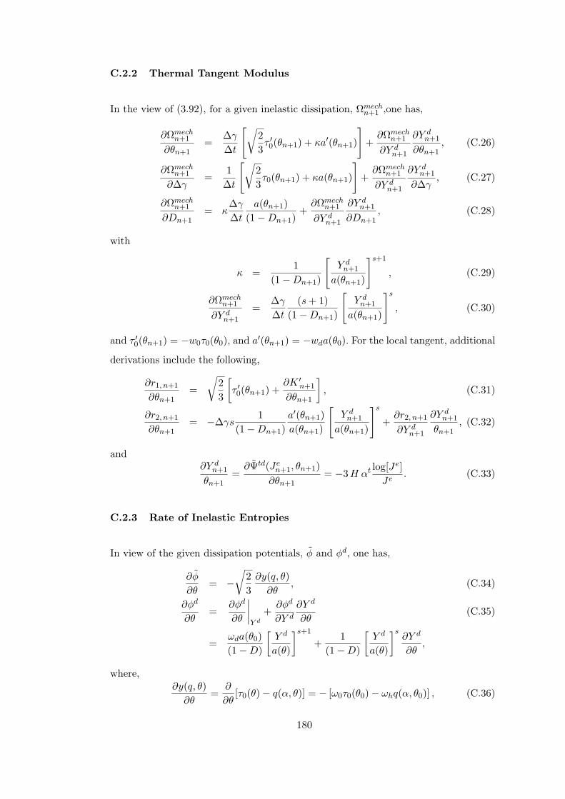
C.2.2 Thermal Tangent Modulus
In the view of (3.92), for a given inelastic dissipation, Ωmechn+1 ,one has,
∂Ωmechn+1
∂θn+1=
∆γ
∆t
[√23τ ′0(θn+1) + κa′(θn+1)
]+
∂Ωmechn+1
∂Y dn+1
∂Y dn+1
∂θn+1, (C.26)
∂Ωmechn+1
∂∆γ=
1∆t
[√23τ0(θn+1) + κa(θn+1)
]+
∂Ωmechn+1
∂Y dn+1
∂Y dn+1
∂∆γ, (C.27)
∂Ωmechn+1
∂Dn+1= κ
∆γ
∆t
a(θn+1)(1−Dn+1)
+∂Ωmech
n+1
∂Y dn+1
∂Y dn+1
∂Dn+1, (C.28)
with
κ =1
(1−Dn+1)
[Y d
n+1
a(θn+1)
]s+1
, (C.29)
∂Ωmechn+1
∂Y dn+1
=∆γ
∆t
(s + 1)(1−Dn+1)
[Y d
n+1
a(θn+1)
]s
, (C.30)
and τ ′0(θn+1) = −w0τ0(θ0), and a′(θn+1) = −wda(θ0). For the local tangent, additional
derivations include the following,
∂r1, n+1
∂θn+1=
√23
[τ ′0(θn+1) +
∂K ′n+1
∂θn+1
], (C.31)
∂r2, n+1
∂θn+1= −∆γs
1(1−Dn+1)
a′(θn+1)a(θn+1)
[Y d
n+1
a(θn+1)
]s
+∂r2, n+1
∂Y dn+1
∂Y dn+1
θn+1, (C.32)
and∂Y d
n+1
θn+1=
∂Ψtd(Jen+1, θn+1)
∂θn+1= −3 H αt log[Je]
Je. (C.33)
C.2.3 Rate of Inelastic Entropies
In view of the given dissipation potentials, φ and φd, one has,
∂φ
∂θ= −
√23
∂y(q, θ)∂θ
, (C.34)
∂φd
∂θ=
∂φd
∂θ
∣∣∣∣Y d
+∂φd
∂Y d
∂Y d
∂θ(C.35)
=ωda(θ0)(1−D)
[Y d
a(θ)
]s+1
+1
(1−D)
[Y d
a(θ)
]s∂Y d
∂θ,
where,∂y(q, θ)
∂θ=
∂
∂θ[τ0(θ)− q(α, θ)] = − [ω0τ0(θ0)− ωhq(α, θ0)] , (C.36)
180

and∂Y d
∂θ=
∂Ψtd
∂θ= −3 H αt log[Je]
Je, (C.37)
Accordingly following time rate of change of the plastic entropy is carried out,
∂ηp
∂t= γ vp
√23
[ω0τ0(θ0)− ωhq(α, θ0)] , (C.38)
which is identical to [162]. The growth of the inelastic entropy associated with damage
is,∂ηd
∂t=
ωda(θ0)(1−D)
[Y d
a(θ)
]s+1
− 3 H αt 1(1−D)
[Y d
a(θ)
]s log[Je]Je
. (C.39)
C.2.4 Plastic Dissipation
Using the proposed von Mises yield potential, one may derive the following equivalence
for the plastic portion of the dissipation expression,
Ωmech,p = τ :[−1
2£vbe • be,−1
]︸ ︷︷ ︸
γ ∂φ∂τ
+q∂α
∂t︸︷︷︸γ ∂φ
∂q
(C.40)
= τ :[
γ
(1−D)s‖s‖
]+ q(α, θ)
[√23γvp
]
= γvp ‖s‖+
√23γvpq(α, θ)
= γvp
√23τ0(θ),
with γvpφ = 0 also τ = τ/(1 − D), τ = p1 + s and p1 : s = 0, and consequently
[τ/(1−D)] : s = s : s = ‖s‖2 .
C.2.5 Thermal State
For the given potentials Ψtd(Je, θ) and Ψt(θ), one may derive the following expressions,
∂Ψtd(Jen+1, θn+1)
∂θn+1= −3 Hαt log[Je]
Je, (C.41)
∂Ψt(θn+1)∂θn+1
= −Cv log[
θ
θ0
]. (C.42)
181

VITA
PERSONAL INFORMATION
Surname, Name: Soyarslan, Celal
Nationality: Turkish (TC)
Date and Place of Birth: 7 December 1977 , Elazıg
Marital Status: Single
Phone: +90 312 586 83 52
Fax: +90 312 586 80 91
email: [email protected]
EDUCATION
Degree Institution Year of Graduation
MS METU, Civil Eng. 2002
BS METU, Civil Eng. 2000
High School Yalova High School, Yalova 1995
WORK EXPERIENCE
Year Place Enrollment
2006-Present Atılım Univ., Manuf. Eng. Instructor
2000-2006 METU, Civil Eng. Research Assistant
FOREIGN LANGUAGES
Advanced English, Intermediate German.
182
PUBLICATIONS
1. Soyarslan, C.; Tekkaya, A. E.; Akyuz, U. [2008]: “Application of Contin-
uum Damage Mechanics in discontinuous crack formation: Forward extrusion chevron
predictions”, Journal of Applied Mathematics and Mechanics / Zeitschrift fur Ange-
wandte Mathematik und Mechanik , Vol. 88, 436–453.
HOBBIES
Reading, Programming, Running, Movies.
183


