
Chapter 9
Modeling and Linear Programming inEngineering Management
William P. Fox and Fausto P. Garcia
Additional information is available at the end of the chapter
http://dx.doi.org/10.5772/54500
1. Introduction
Consider planning the shipment of needed items from the warehouses where they aremanufactured and stored to the distribution centers where they are needed.
There are three warehouses at different cities: Detroit, Pittsburgh and Buffalo. They have 250,130 and 235 tons of paper accordingly. There are four publishers in Boston, New York, Chicagoand Indianapolis. They ordered 75, 230, 240 and 70 tons of paper to publish new books. Thereare the following costs in dollars of transportation of one ton of paper:
From \ To Boston (BS) New York (NY) Chicago (CH) Indianapolis (IN)
Detroit (DT) 15 20 16 21
Pittsburgh (PT) 25 13 5 11
Buffalo (BF) 15 15 7 17
Management wants you to minimize the shipping costs while meeting demand. This probleminvolves the allocation of resources and can be modeled as a linear programming problem aswe will discuss.
In engineering management the ability to optimize results in a constrained environment iscrucial to success. Additionally, the ability to perform critical sensitivity analysis, or “what ifanalysis” is extremely important for decision making. Consider starting a new diet whichneeds to healthy. You go to a nutritionist that gives you lots of information on foods. Theyrecommend sticking to six different foods: Bread, Milk, Cheese, Fish, Potato and Yogurt: andprovides you a table of information including the average cost of the items:
© 2013 Fox and Garcia; licensee InTech. This is an open access article distributed under the terms of theCreative Commons Attribution License (http://creativecommons.org/licenses/by/3.0), which permitsunrestricted use, distribution, and reproduction in any medium, provided the original work is properly cited.
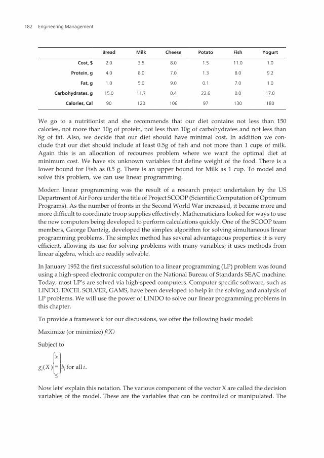
Bread Milk Cheese Potato Fish Yogurt
Cost, $ 2.0 3.5 8.0 1.5 11.0 1.0
Protein, g 4.0 8.0 7.0 1.3 8.0 9.2
Fat, g 1.0 5.0 9.0 0.1 7.0 1.0
Carbohydrates, g 15.0 11.7 0.4 22.6 0.0 17.0
Calories, Cal 90 120 106 97 130 180
We go to a nutritionist and she recommends that our diet contains not less than 150calories, not more than 10g of protein, not less than 10g of carbohydrates and not less than8g of fat. Also, we decide that our diet should have minimal cost. In addition we con‐clude that our diet should include at least 0.5g of fish and not more than 1 cups of milk.Again this is an allocation of recourses problem where we want the optimal diet atminimum cost. We have six unknown variables that define weight of the food. There is alower bound for Fish as 0.5 g. There is an upper bound for Milk as 1 cup. To model andsolve this problem, we can use linear programming.
Modern linear programming was the result of a research project undertaken by the USDepartment of Air Force under the title of Project SCOOP (Scientific Computation of OptimumPrograms). As the number of fronts in the Second World War increased, it became more andmore difficult to coordinate troop supplies effectively. Mathematicians looked for ways to usethe new computers being developed to perform calculations quickly. One of the SCOOP teammembers, George Dantzig, developed the simplex algorithm for solving simultaneous linearprogramming problems. The simplex method has several advantageous properties: it is veryefficient, allowing its use for solving problems with many variables; it uses methods fromlinear algebra, which are readily solvable.
In January 1952 the first successful solution to a linear programming (LP) problem was foundusing a high-speed electronic computer on the National Bureau of Standards SEAC machine.Today, most LP’s are solved via high-speed computers. Computer specific software, such asLINDO, EXCEL SOLVER, GAMS, have been developed to help in the solving and analysis ofLP problems. We will use the power of LINDO to solve our linear programming problems inthis chapter.
To provide a framework for our discussions, we offer the following basic model:
Maximize (or minimize) f(X)
Subject to
gi(X ){≥=≤
}bi for all i.
Now lets’ explain this notation. The various component of the vector X are called the decisionvariables of the model. These are the variables that can be controlled or manipulated. The
Engineering Management182

function, f(X), is called the objective function. By subject to, we connote that there are certainside conditions, resource requirement, or resource limitations that must be met. Theseconditions are called constraints. The constant bi represents the level that the associatedconstraint g (Xi) and is called the right-hand side in the model.
Linear programming is a method for solving linear problems, which occur very frequently inalmost every modern industry. In fact, areas using linear programming are as diverse asdefense, health, transportation, manufacturing, advertising, and telecommunications. Thereason for this is that in most situations, the classic economic problem exists - you want tomaximize output, but you are competing for limited resources. The 'Linear' in Linear Pro‐gramming means that in the case of production, the quantity produced is proportional to theresources used and also the revenue generated. The coefficients are constants and no productsof variables are allowed.
In order to use this technique the company must identify a number of constraints that willlimit the production or transportation of their goods; these may include factors such as laborhours, energy, and raw materials. Each constraint must be quantified in terms of one unit ofoutput, as the problem solving method relies on the constraints being used.
An optimization problem that satisfies the following five properties is said to be a linearprogramming problem.
• There is a unique objective function, f(X).
• Whenever a decision variable, X, appears in either the objective function or a constraintfunction, it must appear with an exponent of 1, possibly multiplied by a constant.
• No terms contain products of decision variables.
• All coefficients of decision variables are constants.
• Decision variables are permitted to assume fractional as well as integer values.
Linear problems, by the nature of the many unknowns, are very hard to solve by humaninspection, but methods have been developed to use the power of computers to do the hardwork quickly. We will illustrate with two variables, graphically.
Supply Chain Management: A company owns railroad freight cars that can be sent all over thecountry. They need to work out what movements will be the most efficient in order to meetcurrent customer needs and future needs on a probability basis, while minimizing time takenand costs incurred.
2. Formulating linear programming problems
A linear programming problem is a problem that requires an objective function to be maxi‐mized or minimized subject to resource constraints. The key to formulating a linear program‐ming problem is recognizing the decision variables. The objective function and all constraintsare written in terms of these decision variables.
Modeling and Linear Programming in Engineering Managementhttp://dx.doi.org/10.5772/54500
183

The conditions for a mathematical model to be a linear program (LP) were:
• all variables continuous (i.e. can take fractional values)
• a single objective (minimize or maximize)
• the objective and constraints are linear i.e. any term is either a constant or a constantmultiplied by an unknown.
• The decision variables must be non-negative
LP's are important - this is because:
• many practical problems can be formulated as LP's
• there exists an algorithm (called the simplex algorithm) that enables us to solve LP's numer‐ically relatively easily.
We will return later to the simplex algorithm for solving LP’s but for the moment we willconcentrate upon formulating LP's.
Some of the major application areas to which LP can be applied are:
• Blending
• Production planning
• Oil refinery management
• Distribution
• Financial and economic planning
• Manpower planning
• Blast furnace burdening
• Farm planning
We consider below some specific examples of the types of problem that can be formulated asLP's. Note here that the key to formulating LP's is practice. However a useful hint is thatcommon objectives for LP's are minimize cost/maximize profit.
Example 1 Manufacturing
Consider the following problem statement:
A company wants to can two new different drinks for the holiday season. It takes 2 hours tocan one gross of Drink A, and it takes 1 hour to label the cans. It takes 3 hours to can one grossof Drink B, and it takes 4 hours to label the cans. The company makes $10 profit on one grossof Drink A and a $20 profit of one gross of Drink B. Given that we have 20 hours to devote tocanning the drinks and 15 hours to devote to labeling cans per week, how many cans of eachtype drink should the company package to maximize profits?
Required Submission for Formulation solution:
Engineering Management184

Problem Identification: Maximize the profit of selling these new drinks.
Define variables:
X1=the number of gross cans produced for Drink A per week
X2= the number of gross cans produced for Drink B per week
Objective Function:
Z=10X1+20X2
1. Canning with only 20 hours available per week
2 X1 + 3 X2 ≤ 20
2. Labeling with only 15 hours available per week
X1 + 4 X2 ≤ 15
3. Non-negativity restrictions
X1≥0 (non-negativity of the production items)
X2≥0 (non-negativity of the production items)
The Complete FORMULATION:
MAXIMIZE Z =10X1+20X2
subject to
2 X1 + 3 X2 ≤ 20
X1 + 4 X2 ≤ 15
X1≥0
X2≥0
We will see in the next section how to solve these two-variable problems graphically.
Example 2 Financial planning
A bank makes four kinds of loans to its personal customers and these loans yield the followingannual interest rates to the bank:
• First mortgage 14%
• Second mortgage 20%
• Home improvement 20%
• Personal overdraft 10%
The bank has a maximum foreseeable lending capability of $250 million and is furtherconstrained by the policies:
1. first mortgages must be at least 55% of all mortgages issued and at least 25% of all loansissued (in $ terms)
2. second mortgages cannot exceed 25% of all loans issued (in $ terms)
Modeling and Linear Programming in Engineering Managementhttp://dx.doi.org/10.5772/54500
185

3. to avoid public displeasure and the introduction of a new windfall tax the average interestrate on all loans must not exceed 15%.
Formulate the bank's loan problem as an LP so as to maximize interest income while satisfyingthe policy limitations.
Note here that these policy conditions, while potentially limiting the profit that the bank canmake, also limit its exposure to risk in a particular area. It is a fundamental principle of riskreduction that risk is reduced by spreading money (appropriately) across different areas.
2.1. Financial planning formulation
Note here that as in all formulation exercises we are translating a verbal description of theproblem into an equivalent mathematical description.
A useful tip when formulating LP's is to express the variables, constraints and objective inwords before attempting to express them in mathematics.
2.2. Variables
Essentially we are interested in the amount (in dollars) the bank has loaned to customers ineach of the four different areas (not in the actual number of such loans). Hence let
xi= amount loaned in area i in a million of dollars (where i=1 corresponds to first mortgages,i=2 to second mortgages etc) and note that each xi >= 0 (i=1,2,3,4).
Note here that it is conventional in LP's to have all variables >= 0. Any variable (X, say) whichcan be positive or negative can be written as X1-X2 (the difference of two new variables) whereX1 >= 0 and X2 >= 0.
2.3. Constraints
a. limit on amount lent
x1 + x2 + x3 + x4≤250
b. policy condition 1
x1≥0.55(x1 + x2)
i.e. first mortgages >= 0.55(total mortgage lending) and also
x1≥0.25(x1 + x2 + x3 + x4)
i.e. first mortgages ≥ 0.25(total loans)
c. policy condition 2
x2≤0.25(x1 + x2 + x3 + x4)Inline formula
Engineering Management186

d. policy condition 3 - we know that the total annual interest is 0.14x1 + 0.20x2 + 0.20x3 +0.10x4 on total loans of (x1 + x2 + x3 + x4). Hence the constraint relating to policy condition(3) is
( )1 2 3 4 1 2 3 40.14 0.20 0.20 0.10 0.15 x x x x x x x x+ + + £ + + + (1)
2.4. Objective function
To maximize interest income (which is given above) i.e.
Maximize Z = 0.14x1 + 0.20x2 + 0.20x3 + 0.10x4
Example 3 Blending and Formulation
Consider the example of a manufacturer of animal feed who is producing feed mix for dairycattle. In our simple example the feed mix contains two active ingredients. One kg of feed mixmust contain a minimum quantity of each of four nutrients as below:
Nutrient A B C D
gram 90 50 20 2
The ingredients have the following nutrient values and cost
A B C D Cost/kg
Ingredient 1 (gram/kg) 100 80 40 10 40
Ingredient 2 (gram/kg) 200 150 20 0 60
What should be the amounts of active ingredients in one kg of feed mix that minimizes cost?
2.5. Blending problem solution
Variables
In order to solve this problem it is best to think in terms of one kilogram of feed mix. Thatkilogram is made up of two parts - ingredient 1 and ingredient 2:
x1= amount (kg) of ingredient 1 in one kg of feed mix
x2= amount (kg) of ingredient 2 in one kg of feed mix
where x1 ≥ 0, x2 ≥ 0
Essentially these variables (x1 and x2) can be thought of as the recipe telling us how to makeup one kilogram of feed mix.
Constraints
• nutrient constraints
Modeling and Linear Programming in Engineering Managementhttp://dx.doi.org/10.5772/54500
187

100x1+ 200x2>= 90 (nutrient A)
80x1+ 150x2>= 50 (nutrient B)
40x1+ 20x2>= 20 (nutrient C)
10x1>= 2 (nutrient D)
• balancing constraint (an implicit constraint due to the definition of the variables)
x1 + x2 = 1
Objective function
Presumably to minimize cost, i.e.
Minimize Z= 40x1+ 60x2
This gives us our complete LP model for the blending problem.
Example 4 Production planning problem
A company manufactures four variants of the same table and in the final part of the manu‐facturing process there are assembly, polishing and packing operations. For each variant thetime required for these operations is shown below (in minutes) as is the profit per unit sold.
Variant 1 Assembly Polish Pack Profit ($)
2 3 2 1.50
2 4 2 3 2.50
3 3 3 2 3.00
4 7 4 5 4.50
Given the current state of the labor force the company estimate that, each year, they have100,000 minutes of assembly time, 50,000 minutes of polishing time and 60,000 minutes ofpacking time available. How many of each variant should the company make per year andwhat is the associated profit?
Variables
Let:
xi be the number of units of variant i (i=1,2,3,4) made per year, where xi ≥ 0 i=1,2,3,4
Constraints
Resources for the operations of assembly, polishing, and packing
2x1+ 4x2+ 3x3+ 7x4<=100,000 (assembly)
3x1+ 2x2+ 3x3+ 4x4< = 50,000 (polishing)
2x1+ 3x2+ 2x3+ 5x4< = 60,000 (packing)
Objective function
Engineering Management188

Maximize Z= 1.5x1+ 2.5x2+ 3.0x3+ 4.5x4
Example 5 Shipping
Consider planning the shipment of needed items from the warehouses where they are manufac‐tured and stored to the distribution centers where they are needed as shown in the introduc‐tion. There are three warehouses at different cities: Detroit, Pittsburgh and Buffalo. They have250, 130 and 235 tons of paper accordingly. There are four publishers in Boston, New York,Chicago and Indianapolis. They ordered 75, 230, 240 and 70 tons of paper to publish new books.
There are the following costs in dollars of transportation of one ton of paper:
From \ To Boston (BS) New York (NY) Chicago (CH) Indianapolis (IN)Detroit (DT) 15 20 16 21
Pittsburgh (PT) 25 13 5 11Buffalo (BF) 15 15 7 17
Management wants you to minimize the shipping costs while meeting demand.
We define xij to be the travel from city i (1 is Detroit, 2 is Pittsburg, 3 is Buffalo) to city j (1 isBoston, 2 is New York, 3 is Chicago, and 4 is Indianapolis).
Minimize Z= 15x11+20x12+16x13+21x14+25x21+13x22+5x23+11x24+15x31+15x32+7x33+17x34
Subject to:
x11+x12+x13+x14≤250 (availability in Detroit)
x21+x22+x23+x24≤130 (availability in Pittsburg)
x31+x32+x33+x34≤235 (availability in Buffalo)
x11+x21+x31≥ 75 (demand Boston)
x12+x22+x32≥230 (demand New York)
x13+x23+x334≥240 (demand Chicago)
x14+x24+x34≥70 (demand Indianapolis)
xij≥0
3. LP geometry
Many applications in business and economics involve a process called optimization. Inoptimization problems, you are asked to find the minimum or the maximum result. Thissection illustrates the strategy in graphical simplex of linear programming. We will restrictourselves in this graphical context to two-dimensions. Variables in the simplex method arerestricted to positive variables (for example x ≥ 0).
Modeling and Linear Programming in Engineering Managementhttp://dx.doi.org/10.5772/54500
189

A two-dimensional linear programming problem consists of a linear objective function and asystem of linear inequalities called constraints. The objective function gives the linear quantitythat is to be maximized (or minimized). The constraints determine the set of feasible solutions.
Memory chips for CPUs
Let’s start with a manufacturing example. Suppose a small business wants to know how manyof two types of high-speed computer chips to manufacturer weekly to maximize their profits.First, we need to define our decision variables. Let,
x1= number of high speed chip type A to produce weekly
x2= number of high speed chip type B to produce week
The company reports a profit of $140 for each type A chip and $120 for each type B chip sold.The production line reports the following information:
Chip A Chip B Quantity availableAssembly time (hours) 2 4 1400
Installation time (hours) 4 3 1500Profit ( per unit) 140 120
The constraint information from the table becomes inequalities that are written mathematicalas:
2x1+ 4x2≤1400 (assembly time)
4x1+ 3x2≤1500 (installation time)
x1≥0, x2≥0
The profit equation is:
Profit = 140x1+ 120x2
The feasible region
The constraints of a linear program, which include any bounds on the decision variables,essentially shape the region in the x-y plane that will be the domain for the objective functionprior to any optimization being performed. Every inequality constraint that is part of theformulation divides the entire space defined by the decision variables into 2 parts: the portionof the space containing points that violate the constraint, and the portion of the space contain‐ing points that satisfy the constraint.
It is very easy to determine which portion will contribute to shaping the domain. We can simplysubstitute the value of some point in either half-space into the constraint. Any point will do, butthe origin is particularly appealing. Since there's only one origin, if it satisfies the constraint,then the half-space containing the origin will contribute to the domain of the objective function.
When we do this for each of the constraints in the problem, the result is an area representingthe intersection of all the half-spaces that satisfied the constraints individually. This intersection
Engineering Management190

is the domain for the objective function for the optimization. Because it contains points that
satisfy all the constraints simultaneously, these points are considered feasible to the problem.
Naturally, the common name for this domain is the feasible region.
Consider our constraints:
2x1+ 4x2≤1400 (assembly time)
4x1+ 3x2≤1500 (installation time)
x1≥0,x2≥0
For our graphical work we use the constraints: x1 ≥ 0, x2 ≥ 0 to set the region. Here, we are
strictly in the x1-x2 plane (the first quadrant).
Let’s first take constraint #1 (assembly time) in the first quadrant: 2x1 + 4x2 ≤ 1400
Figure 1. Shaded Inequality
We see the shaded region for constraint 1 that makes the inequality true. We repeat this process
for all constraints to obtain Figure 2.
Modeling and Linear Programming in Engineering Managementhttp://dx.doi.org/10.5772/54500
191

Figure 2. Plot of (1) the assembly hour’s constraint and (2) the installation hour’s constraint in the first quadrant
Figure 2 shows a plot of (1) the assembly hour’s constraint and (2) the installation hour’sconstraint in the first quadrant. Along with the non-negativity restrictions on the decisionvariables, the intersection of the half-spaces defined by these constraints is the feasible regionshown in yellow. This area represents the domain for the objective function optimization.
Finding the feasible region
Shade in the feasible region defined by the following set of constraints:
x+ 2y≤202x+y≤20x≥0,y≥0
The feasible region is the set of ordered pairs (x, y) that satisfy all four constraints simultane‐ously. They are points that lie below x + 2y ≤ 20, below 2x+y ≤ 20, and above y = 0 and to theright of x=0. We note that the non-negativity constraints, x ≥ 0, y ≥ 0, restrict the feasible regionto the first quadrant. ≤
If the problem is well behaved, this should be a closed and bounded polyhedral shape, calleda polyhedron, such as the one shown in yellow. It does not have to be so. Sometimes theorientation and location of the constraints fail to hold back the objective function in thedirection of the optimization. When this happens, the problem is unbounded; the objective
Engineering Management192

function value goes off to positive or negative infinity. Can you draw a sketch of a situationin which this will happen?
Other times, the intersection of the half-spaces is an empty set. In this case, the problem isinfeasible; there are no possible solutions that will satisfy the requirements of all the constraintssimultaneously. Can you draw a sketch of a situation in which this will happen?
3.1. Solving a linear programming problem graphically
Recall that we have decision variables defined and an objection function that is to be maximizedor minimized. Although all points inside the feasible region provide feasible solutions thesolution, if one exists, occurs according to the Fundamental Theorem of Linear Programming:
If the optimal solution exists, then it occurs at a corner point of the feasible region.
Notice the various corners formed by the intersections of the constraints in example. Thesepoints are of great importance to us. There is a cool theorem (didn't know there were any ofthese, huh?) in linear optimization that states, "if an optimal solution exists, then an optimalcorner point exists." The result of this is that any algorithm searching for the optimal solutionto a linear program should have some mechanism of heading toward the corner point wherethe solution will occur. If the search procedure stays on the outside border of the feasible region
Figure 3. Shaded Feasible Region
Modeling and Linear Programming in Engineering Managementhttp://dx.doi.org/10.5772/54500
193

while pursuing the optimal solution, it is called an exterior point method. If the search procedurecuts through the inside of the feasible region, it is called an interior point method.
Thus, in a linear programming problem, if there exists a solution, it must occur at a cornerpoint of the set of feasible solutions (these are the vertices of the region). Note that in Figure3 the corner points of the feasible region are the coordinates: (0,0), (0,10) (10, 0), and (20/3, 20/3).
How did we get the point (20/3, 20/3)?
This point is the intersection of the lines: x + 2y = 20 and 2x+y=20. You have solved theseproblems before. In the second constraint, let y = 20-2x and substitute (20-2x) for y in the firstequation, so x + 2(20-2x) = 20 and solve for x. We find 3x = 20 or x =20/3. Since y = 20-2x, wesubstitute x = 20/3 for x and solve for y. Now, y =20/3.
Now, that we have all the possible solution coordinates for (x, y), we need to know which isthe optimal solution. Here is how we determine that:
We evaluate the objective function at each point and choose the best solution.
Assume our objective function is to Maximize Z = 2 x + 2y. We can set up a table of coordinatesand corresponding Z-values as follows.
Coordinate of Corner Point Z= 2x + 2y
(0,0) Z= 0
(0,10) Z = (2)(0) + (2)(10) =20
(20/3, 20/3) Z=(2)(20/3)+(2)(20/3)= 80/3 *
(10,0) Z = (2)(10) + (2)(0)= 20
Best solution is (20/3,20/3) Z =80/3=26.666
Graphically, we see the result by plotting the objective function line, Z = 2x + 2y, with thefeasible region. Determine the parallel direction for the line to maximize (in this case) Z. Movethe line parallel until it crosses the last point in the feasible set. That point is the solution. Theline that goes through the origin at a slope of -2/2 is called the ISO-Profit line. We have providedthis Figure 4 below:
Here are the steps for solving a linear programming problem involving only two variables.
Engineering Management194

1. Sketch the region corresponding to the system of constraints. The points satisfying allconstraints make up the feasible solution.
2. Find all the corner points (or intersection points in the feasible region).
3. Test the objective function at each corner point and select the values of the variables thatoptimize the objective function. For bounded regions, both a maximum and a minimumwill exist. For an unbounded region, if a solution exists, it will exist at a corner.
3.2. Minimization problem
Minimize Z = 5 x + 7y
Subject to:
2 x + 3 y≥63 x - y≤15-x + y≤42x + 5y≤27x≥0y≥0
Figure 4. Iso-Profit Lines Added
Modeling and Linear Programming in Engineering Managementhttp://dx.doi.org/10.5772/54500
195

The corner points in Figure 5 are (0,2), (0,4,) (1,5), (6,3), (5,0), and (3,0). See if you can find allthese corner points.
If we evaluate Z = 5x + 7y at each of these points, we find:
Corner Point Z = 5x + 7y (MINIMIZE)
(0,2) Z=14
(1,5) Z= 40
(6,3) Z= 51
(5,0) Z=25
(3,0) Z=15
(0,4) Z=28
The minimum value occurs at (0, 2) with a Z value of 14. Notice in our graph that the blue ISO-Profit line will last cross the point (0,2) as it move out of the feasible region in the direction thatMinimizes Z.
Engineering Management196

3.3. Unbounded case
Let's examine the concept of an unbounded feasible region. Look at the constraints:
x + 2 y≥43 x + y≥7x≥0 and y≥0
Note that the corner points are (0, 7), (2, 1) and (4, 0) and the region is unbounded. If our solutionis to Minimize Z=x+y then our solution is: (2, 1) with Z =3. Determine why there is no solutionto the LP to Maximize Z = x + y.
4. Graphical sensitivity analysis
One of the most important topics in linear programming is sensitivity analysis. In this sectionwe illustrate the concept of sensitivity analysis through a graphical example. Sensitivityanalysis is concerned with how changes in the parameters (coefficient and right-hand-sidevalues) affect the LP’s optimal solution. Very often, we can ascertain whether the optimalsolution variables remain the same (perhaps with different solution values) or whether thevariables will change.
Modeling and Linear Programming in Engineering Managementhttp://dx.doi.org/10.5772/54500
197

Reconsider the following example:
Maximize 2x+ 2y
Subject to:
x+ 2y≤202x+y≤20x≥0,y≥0
The corners of the feasible region with the respective objective function values are shown inthe following table:
Point Coordinates Z-Value
A (0,0) Z=0
B (10,0) Z=20
C (0,10) Z=20
D (20/3,20/3) Z= 80/3=26.66666 Optimal
The optimal solution is currently x= 20/3, y = 20/3 and Z = 80/3.
Engineering Management198

4.1. Graphical analysis of the effect of an objective function coefficient
Recall our objective function:
Z= 2x+ 2y
The slope of this objective function line is –1. The solution is currently at Point D, the coordi‐nates (20/3, 20/3). Recall that the optimal solution, if it exists, must lie at the corner point of thefeasible region. The next closest points to D are B and C. B lies on constraint (2) and C lies onconstraints (1). The slope of constraint (1) is –1/2 and the slope of constraint (2) is –2.
You can see that if we change the coefficients, let say, A x + 2 y, its slope is –A/2. Currently, Ais 2 with a slope of –1. The bounds for the slope to retain Point D as a solution is between –2≤ slope≤ –1/2 (Note at equality we will have alternate optimal solutions). We can easily solvefor the values of A that keep the slope within its bounds. 1≤A≤4. Since A is currently 2, it candecrease by 1 unit or increase by 2 units and still keep Point D optimal.
Let’s try 2 x + by with its slope –2/b. Currently, B is 2 with a slope of –1. The bounds for theslope to retain Point D as a solution is between –2 ≤ slope≤ –1/2 (Note at equality we will havealternate optimal solutions). We can easily solve for the values of B that keep the slope withinits bounds. 1≤B≤4. Since B is currently 2, it can decrease by 1 unit or increase by 2 units andstill keep Point D optimal.
4.2. Graphical analysis of the effect of a change in a right-hand side coefficient
The right-hand side value for each constraint controls the y-intercept of the problem. The slopeswill remain the same. Changing the right-hand side yields a parallel line to the originalconstraint. Point D is the intersection of constraints (1) and (2). Points B and C are the inter‐sections of constraints (1) and Constraint (2) each with non-negativity.
Let’s consider constraint (1), x+ 2y ≤ B
The value of B is currently 20. If it is reduced then the line moves down until it intersects point(10, 0). Using (10, 0) in the equation yields a B value of 10. If we increase B, then we move upto an original infeasible point (0, 20), which will now become feasible. Using (0, 20) in theequation yields a B value of 40.
Thus, 10≤B≤40. This is a decrease of 10 units and an increase of 20 units.
Let’s consider constraint (2), 2x + y ≤ C
The value of C is currently 20. If it is reduced then the line moves down until it intersects point(0, 10). Using (0, 10) in the equation yields a C value of 10. If we increase C, then we move upto an original infeasible point (20, 0), which will now become feasible. Using (20, 0) in theequation yields a C value of 40.
Thus, 10≤C≤40. This is a decrease of 10 units and an increase of 20 units.
Maximize Z= 20x1+30 x2
Subject to:
Modeling and Linear Programming in Engineering Managementhttp://dx.doi.org/10.5772/54500
199

2x1+ 4x3≤1400 (assembly time)
4x1+ 3x3≤1500 (installation time)
The solution is (180,260), Z =11400.
Let’s see the effects of changing the coefficients of the objective function since managementhas some leeway with the revenues and costs
Z= 20x1+ 30x2
The slope of this objective function line is –2/3. The solution is currently at Point D, thecoordinates (180,260). Recall that the optimal solution, if it exists, must lie at the corner pointof the feasible region. The next closest points to D are B and C. B lies on constraint (2) and Clies on constraints (1). The slope of constraint (1) is –1/2 and the slope of constraint (2) is –4/3.
You can see that if we change the coefficients, let say, A x1 + 30 x2, its slope is –A/30. Currently,A is 20 with a slope of –2/3. The bounds for the slope to retain Point D has a solution between–4/3 ≤ slope≤ –1/2. We can easily solve for the values of A that keep the slope within its bounds.15≤A≤40. Since A is currently 20, it can decrease by 5 units or increase by 20 units and still keepPoint D optimal.
Now, let’s try changing the coefficient of the other variable: 20 x + B y with its slope –20/B.Currently, B is 30 with a slope of –2/3. The bounds for the slope to retain Point D as a solutionis between –4/3 ≤ slope≤ –1/2 We can easily solve for the values of B that keep the slope within
Engineering Management200

its bounds. 15≤B≤40. Since B is currently 30, it can decrease by 15 units or increase by 10 unitsand still keep Point D optimal.
5. The simplex method
In the previous sections we discussed formulating linear programming problems, solving two-dimensional linear programming problems by graphical methods, and graphical sensitivityanalysis. The graphical method illustrates some key concepts, but is only practical for problemswith two variables. As you see linear programming problems often have more than twovariables. With problems with more than two variables, an algebraic method may be used.This method is called the Simplex Method. The Simplex Method, developed by George Dantzigin 1947 incorporates both optimality and feasibility tests to find the optimal solution(s) to a linearprogram (if one exists).
An optimality test shows whether or not an intersection point corresponds to a value of theobjective function better than the best value found so far.
A feasibility test determines whether the proposed intersection point is feasible. It does notviolate any of the constraints.
Modeling and Linear Programming in Engineering Managementhttp://dx.doi.org/10.5772/54500
201

The simplex method starts with the selection of a corner point (usually the origin if it is afeasible point) and then, in a systematic method, moves to adjacent corner points of the feasibleregion until the optimal solution is found or it can be shown that no solution exists.
5.1. Steps of the simplex method
1. Tableau Format: Place the linear program in Tableau Format, as explained below.
Maximize Z = 25x1+30x2
Subject to:
20x1+30x2≤6905x1+4x2≤120x1, x2,≥0
To begin the simplex method, we start by converting the inequality constraints (of the form <)to equality constraints. This is accomplished by adding a unique, non-negative variable, calleda slack variable, to each constraint. For example the inequality constraint 20x1+30x2 ≤ 690 isconverted to an equality constraint by adding the slack variable S1 to obtain:
20x1+30x2+S1= 690, where S1≥0.
The inequality 20x1+30x2 ≤ 690 states that the sum 20x1+30x2 is less than or equal to 690. Theslack variable “takes up the slack” between the values used for x1 and x2 and the value 690. Forexample, if x1=x2 =0, the S1 =690. If x1=24, x2=0 then 20(24) +30(0) +S1=690, so S1 = 210.
A unique slack variable must be added to each inequality constraint.
Maximize Z = 25x1+30x2
Subject to:
20x1+30x2+S1= 6905x1+4x2+S2=120x1≥0, x2≥0, S1≥0, S2≥0
Adding slack variables makes the constraint set a system of linear equations. We write thesewith all variables on the left side of the equation and all constants on the right hand side.
We will even rewrite the objective function by moving all variables to the left-hand side.
Maximize Z = 25x1+30x2 is written as
Z- 25x1-30x2=0
Now, these can be written in the following form:
Z- 25x1-30x2 = 020x1+30x2+S1 = 6905x1+4x2+S2=120
Engineering Management202

or more simply in a matrix. This matrix is called the simplex tableau.
Z x1 x2 S1 S2 RHS
1 -25 -30 0 0 = 0
0 20 30 1 0 = 690
0 5 4 0 1 = 120
2. Initial Extreme Point: The Simplex Method begins with a known extreme point, usually theorigin (0, 0) for many of our examples. The requirement for a basic feasible solution givesrises to special Simplex methods such as Big M and Two-Phase Simplex, which can bestudied in a linear programming course.
The Tableau previously shown contains the corner point (0, 0) is our initial solution.
Z x1 x2 S1 S2 RHS
1 -25 -30 0 0 = 0
0 20 30 1 0 = 690
0 5 4 0 1 = 120
We read this solution as follows:
x1= 0x2= 0S1=690S2=120Z=0
Let’s continue to define a few of these variables further. We have 5 variables {Z, x1, x2, S1, S2}and 3 equations. We can have at most 3 solutions. Z will always be a solution by conventionof our tableau. We have two non-zero variables among {x1, x2, S1, S2}. These non-zero variablesare called the basic variables. The remaining variables are called the non-basic variables. Thecorresponding solutions are called the basic feasible solutions (FBS) and correspond to cornerpoints. The complete step of the simplex method produces a solution that corresponds to acorner point of the feasible region. These solutions are read directly from the tableau matrix.
We also note the basic variables are variables that have a column consisting of one 1 and therest zeros in their column. We will add a column to label these as shown below:
Basic
Variable
Basic variableBasic variable
Z x1 x2 S1 S2 RHS
Z 1 -25 -30 0 0 = 0
Modeling and Linear Programming in Engineering Managementhttp://dx.doi.org/10.5772/54500
203

Basic
Variable
Basic variableBasic variable
S1 0 20 30 1 0 = 690
S2 0 5 4 0 1 = 120
3. Optimality Test: We need to determine if an adjacent intersection point improves the valueof the objective function. If not, the current extreme point is optimal. If an improvementis possible, the optimality test determines which variable currently in the independent set(having value zero) should enter the dependent set as a basic variable and become nonzero.For our maximization problem, we look at the Z-Row (The row marked by the basicvariable Z). If any coefficients in that row are negative then we select the variable whosecoefficient is the most negative as the entering variable.
Basic
Variable
Basic variableBasic variable
Z x1 x2 S1 S2 RHS
Z 1 -25 -30 0 0 = 0
S1 0 20 30 1 0 = 690
S2 0 5 4 0 1 = 120
In the Z-Row the coefficients are:
Z x1 x2 S1 S2
Z 1 -25 -30 0 0
The variable with the most negative coefficient is x2 with value –30. Thus, x2 wants to becomea basic variable. We can only have three basic variables in this example (because we have threeequations) so one of the current basic variables {S1, S2} must be replaced by x2. Let’s proceedto see how we determine which variable exists being a basic variable.
4. Feasibility Test: To find a new intersection point, one of the variables in the basic variableset must exit to allow the entering variable from Step 3 to become basic. The feasibility testdetermines which current dependent variable to choose for exiting, ensuring we stayinside the feasible region. We will use the minimum positive ratio test as our feasibilitytest. The Minimum Positive Ratio test is the MIN( RHSj/aj > 0). Make a quotient of therh sj
aj.
Engineering Management204

Most negative
coefficient (-30)
Ratio Test
Z x1 x2 S1 S2 RHS Quotient
Z 1 -25 -30 0 0 = 0
S1 0 20 30 1 0 = 690 690/30=23
S2 0 5 4 0 1 = 120 120/4=30
Note that we will always disregard all quotients with either 0 or negative values in thedenominator. In our example we compare {23, 30} and select the smallest non-negative value.This gives the location of the matrix pivot that we will perform.
Most negative
coefficient (-30)
Ratio Test
Z x1 x2 S1 S2 RHS Quotient
Z 1 -25 -30 0 0 = 0
S1 0 20 30 Pivot 1 0 = 690 690/30=23
S2 0 5 4 0 1 = 120 120/4=30
5. Pivot: We can form a new equivalent system by using row operations to change the pivotelement to a 1 and all other numbers in the pivot column to zero. We do the row operationsby adding a suitable multiple of the pivot row to a multiple of each row in the tableau,thus eliminating the new basic variable. Then set the new non-basic variables to zero inthe new system to find the values of the new basic variables, thereby determining anintersection point.
Pivot
Column
Z x1 x2 S1 S2 RHS
Z 1 -25 -30 0 0 = 0
S1 0/30 20/30 30/30 1/30 0/30 = 690/30 Pivot Row
S2 0 5 4 0 1 = 120
Modeling and Linear Programming in Engineering Managementhttp://dx.doi.org/10.5772/54500
205

Make the entry in the intersection of the pivot column and pivot row equal to 1.
Pivot
Column
Z x1 x2 S1 S2 RHS
Z 1 -25 -30 0 0 = 0
S1 0 2/3 1 1/30 0/ = 23 Pivot Row
S2 0 5 4 0 1 = 120
Using row operations make all other entries in the pivot column equal to 0.
Pivot Column
Z x1 x2 S1 S2 RHS
Z 1 -5 0 1 0 = 690 30R2+R1 àR1
x2 0 2/3 1 1/30 0 = 23
S2 0 7/3 0 -4/30 1 = 28 -4R2+R3 àR3
Let’s interpret our current basic feasible solution.
Basic Variables:
x2=23S2=32Z= 690
Non-Basic Variables x1 = 0, S1 =0
6. Repeat Steps 3-5 until an optimal extreme point is found.
We note that x1 has a coefficient of –5 in the Z-Row therefore, we are not optimal.
Step 3.
Negative
Coefficient
Z x1 X2 S1 S2 RHS
Z 1 -5 0 1 0 = 690
x2 0 2/3 1 1/30 0 = 23
S2 0 7/3 0 -4/30 1 = 28
Engineering Management206

Step 4.
Pivot
Column
Ratio Test
Z x1 x2 S1 S2 RHS Quotient
Z 1 -5 0 1 0 = 690
x2 0 2/3 1 1/30 0 = 23 69/2=34.5
S2 0 7/3 0 -4/30 1 = 28 84/7=12* Min
The minimum non-negative quotient is 12. This indicates that to remain in the feasible region
that x1 enters as a basic variable and S2 leaves being a basic variable.
Pivot
Column
Ratio Test
Z x1 x2 S1 S2 RHS Quotient
Z 1 -5 0 1 0 = 690
x2 0 2/3 1 1/30 0 = 23
S2 0 7/3 0 -4/30 1 = 28 Pivot Row
Step 5. We make the highlighted position a 1 and all other column entries 0 for the column of
x1. We divide the entire S2 row by 7/3.
Z x1 x2 S1 S2 RHS
Z 1 -5 0 1 0 = 690
x2 0 2/3 1 1/30 0 = 23
S2 0 1 0 -12/210 3/7 = 12
Z x1 x2 S1 S2 RHS
Z 1 0 0 5/7 15/7 = 750 5R3+R1 àR1
x2 0 0 1 1/14 -2/7 = 15 -2/3R3+R2 àR2
x1 0 1 0 -2/35 3/7 = 12
Modeling and Linear Programming in Engineering Managementhttp://dx.doi.org/10.5772/54500
207

The current solution is read as follows:
Basic Variables
x2= 15x1= 12Z = 750
Non-basic variables
S1=S2=0
There are no negative coefficients in the Z-Row, so we are optimal.
Z x1 x2 S1 S2
Z 1 0 0 5/7 15/7
Figure 5. The set of points satisfying the constraint of this linear programming problem (the convex set as a shadedregion)
Engineering Management208

Each solution found in the tableau corresponds to a corner point. We went from corner (0, 0)to corner (0, 23) to corner (12, 15).
Maximize Z=3x1+x2
Subject to:
2x1+ x2≤6x1+ 3x2≤9x1, x2≥0
The Tableau Format with slack variables y1, y2:
Basic Var. Z x1 x2 y1 y2 RHS
Z 1 -3 -1 0 0 0
y1 0 2 1 1 0 6
y2 0 1 3 0 1 9
Basic variable {Z, y1, y2}
Non-basic Variable {x1, x2}
Extreme Point (0, 0) ---Corresponding to the values of (x1, x2)
Value of objective function: Z=0
Optimality Test: The entering variable is x1 (corresponding to -3 in the Z- row.)
Feasibility Test: Compute the ratios of the ``RHS'' divided by the column labeled x1 to deter‐mine the minimum positive ratio.
Basic Var. Z x1 x2 y1 y2 RHS Quotient
Z 1 -3 -1 0 0 0
y1 0 2 1 1 0 6 6/2=3
y2 0 1 3 0 1 9 9/1=9
Choose y1 to leave since it corresponds to the minimum positive ratio test value of 3.
Pivot: Divide the row containing the exiting variable (the first row in this case) by the coefficientof the entering variable in that row (the coefficient of x1 in this case), giving a coefficient of 1for the entering variable in this row. Then eliminate the entering variable x1 from the remainingrows (which do not contain the exiting variable y1 and have a zero coefficient for it). The resultsare summarized in the next tableau.
Modeling and Linear Programming in Engineering Managementhttp://dx.doi.org/10.5772/54500
209

Basic Var. Z x x2 y1 y2 RHS
Z 1 0 0.5000 1.5 0 9
x1 0 1 0.5000 .5 0 3
y2 0 0 2.5000 -.5 1 6
Basic variable {Z, x1, y2}
Non-basic Variable {y1, x2}
Extreme Point (3, 0) ---Corresponding to the values of (x1, x2)
Value of objective function: Z=9
The pivot determines that the dependent variables have the values x1=3, y2=6 and Z=9.
Optimality Test: There are no negative coefficients in the Z- row. Thus x1=3 (a basic variable)and x2=0 (a non-basic variable) is an extreme point giving the optimal objective function valueZ=9.
We read the solution as Z=9, x1=3, and s2=6.
Remarks: We have assumed that the origin is a feasible extreme point. If it is not, then an extremepoint must be found before the Simplex Method, as presented, can be used. We have alsoassumed that the linear program is not ``degenerate'' in the sense that no more than twoconstraints intersect at the same point. These and other topics are studied in more advancedoptimization courses.
6. Linear programming with technology
Technology is critical to solving, analyzing, and performing sensitivity analysis on linearprogramming problems. Technology provides a suite of powerful, robust routines for solvingoptimization problems, including linear programs (LPs). Technology, that we briefly discuss,includes Excel, LINDO, and LINGO as these appear to be used often in engineering. We testedall these software packages and found them useful.
We present our previous example solved via each technology.
Maximize Z = 25x1+30x2
Subject to:
20x1+30x2≤6905x1+4x2≤120x1, x2,≥0
Engineering Management210

EXCEL
Modeling and Linear Programming in Engineering Managementhttp://dx.doi.org/10.5772/54500
211

Solver
Constraints into solver
Engineering Management212

Reports
Answer Report
Modeling and Linear Programming in Engineering Managementhttp://dx.doi.org/10.5772/54500
213

Sensitivity Report
We find our solution is x1=9, x2=24, P=$972. From the standpoint of sensitivity analysis Excelis satisfactory in that it provides shadow prices.
Limitation: No tableaus are provided making it difficult to find alternate solutions.
Engineering Management214

LINDO
MAX 25 X1 + 30 X2 SUBJECT TO 2) 20 X1 + 30 X2 <= 690 3) 5 X1 + 4 X2 <= 120 END
THE TABLEAU ROW (BASIS) X1 X2 SLK 2 SLK 3 1 ART -25.000 -30.000 0.000 0.000 0.000 2 SLK 2 20.000 30.000 1.000 0.000 690.000 3 SLK 3 5.000 4.000 0.000 1.000 120.000 ART ART -25.000 -30.000 0.000 0.000 0.000
LP OPTIMUM FOUND AT STEP 2 OBJECTIVE FUNCTION VALUE 1) 750.0000
VARIABLE VALUE REDUCED COST X1 12.000000 0.000000 X2 15.000000 0.000000
ROW SLACK OR SURPLUS DUAL PRICES 2) 0.000000 0.714286 3) 0.000000 2.142857
NO. ITERATIONS= 2
RANGES IN WHICH THE BASIS IS UNCHANGED: OBJ COEFFICIENT RANGES
VARIABLE CURRENT ALLOWABLE ALLOWABLE
COEF INCREASE DECREASE X1 25.000000 12.500000 5.000000 X2 30.000000 7.500000 10.000000
RIGHTHAND SIDE RANGES
ROW CURRENT ALLOWABLE ALLOWABLE
RHS INCREASE DECREASE 2 690.000000 210.000000 209.999985 3 120.000000 52.499996 28.000000
THE TABLEAU
ROW (BASIS) X1 X2 SLK 2 SLK 3 1 ART 0.000 0.000 0.714 2.143 750.000 2 X2 0.000 1.000 0.071 -0.286 15.000 3 X1 1.000 0.000 -0.057 0.429 12.000
Modeling and Linear Programming in Engineering Managementhttp://dx.doi.org/10.5772/54500
215

LINGO
MODEL:
MAX = 25 * x1 + 30 * x2;
20 * x1 + 30 * x2 <= 690; 5 * x1 + 4 * x2 <= 120; x1>=0; x2>=0;
END
Variable Value Reduced Cost X1 12.00000 0.0000000 X2 15.00000 0.0000000
Row Slack or Surplus Dual Price 1 750.0000 1.000000 2 0.0000000 0.7142857 3 0.0000000 2.142857 4 12.00000 0.0000000 5 15.00000 0.0000000
7. Case study
In our case study we present linear programming for supply chain design. We considerproducing a new mixture of gasoline. We desire to minimize the total cost of manufacturingand distributing the new mixture. There is a supply chain involved with a product that mustbe modeled. The product is made up of components that are produced separately.
Crude Oil type Compound A (%) Compound B (%) Compound C (%) Cost/Barrel Barrel Avail (000
of barrels)
X10 35 25 35 $26 15000
X20 50 30 15 $32 32000
X30 60 20 15 $55 24000
Demand information is as follows:
Gasoline Compound A (%) Compound B (%) Compound C (%) Expected Demand
(000 of barrels)
Premium ≥ 55 ≤23 14000
Super ≥25 ≤35 22000
Regular ≥40 ≤25 25000
Engineering Management216

Let i = crude type 1, 2, 3 (X10,X20,X30 respectively)Let j = gasoline type 1, 2, 3 (Premium, Super, Regular respectively)
We define the following decision variables:
Gij= amount of crude i used to produce gasoline j
For example,
G11= amount of crudeX10used to produce Premium gasoline.G12= amount of crude typeX20used to produce Premium gasolineG13= amount of crude typeX30used to produce Premium gasolineG12= amount of crude typeX10used to produce Super gasolineG22= amount of crude typeX20used to produce Super gasolineG32= amount of crude typeX30used to produce Super gasolineG13= amount of crude typeX10used to produce Regular gasolineG23= amount of crude typeX20used to produce Regular gasolineG33= amount of crude typeX30used to produce Regular gasoline
LP formulation
Minimize Cost= $86 (G11+G21+G31)+$92(G12+G22+G32)+$95(G13+G23+G33)
Subject to: Demand
G11+G21+G31>14000 (Premium)G12+G22+G32>22000 (Super)G13+G23+G33>25000 (Regular)
Availability of products
G11+G12+G13 < 15000 (crude 1)G21+G22+G23 < 32000 (crude 2)G31+G32+G33 < 24000 (crude 3)
Product mix in mixture format
(0.35 G11 + 0.50 G21 + 0.60 G31) / (G11 + G21 + G31)≥ 0.55 (X 10 in Premium)(0.25 G11 + 0.30 G21 + 0.20 G31) / (G11 + G21 + G31)≤0.23 (X 20 in Premium)(0.35 G13 + 0.15 G23 + 0.15 G33) / (G13 + G23 + G33)≥0.25 (X 20 in Regular)(0.35 G13 + 0.15 G23 + 0.15 G33) / (G13 + G23 + G33)≤0.35 (X 30 in Regular)(0.35G12 + 0.50G22 + 0.60 G23) / (G12 + G22 + G32)≤0.40 (Compound X 10 in Super)(0.35G12 + 0.15G22 + 0.15 G32) / (G12 + G22 + G32)≤0.25 (Compound X 30 in Super)
The solution was found using LINDO and we noticed an alternate optimal solution. Twosolutions are found yielding a minimum cost of $1,904,000.
Modeling and Linear Programming in Engineering Managementhttp://dx.doi.org/10.5772/54500
217

Decision variable Z=$1,940,000 Z=$1,940,000
G11 0 1,400
G12 0 3,500
G13 14,000 9,100
G21 15,000 1,100
G22 7,000 20,900
G23 0 0
G31 0 12,500
G32 25,000 7,500
G33 0 4,900
Depending on whether we want to additionally minimize delivery (across different locations)
or maximize sharing by having more distribution point involved then we have choices.
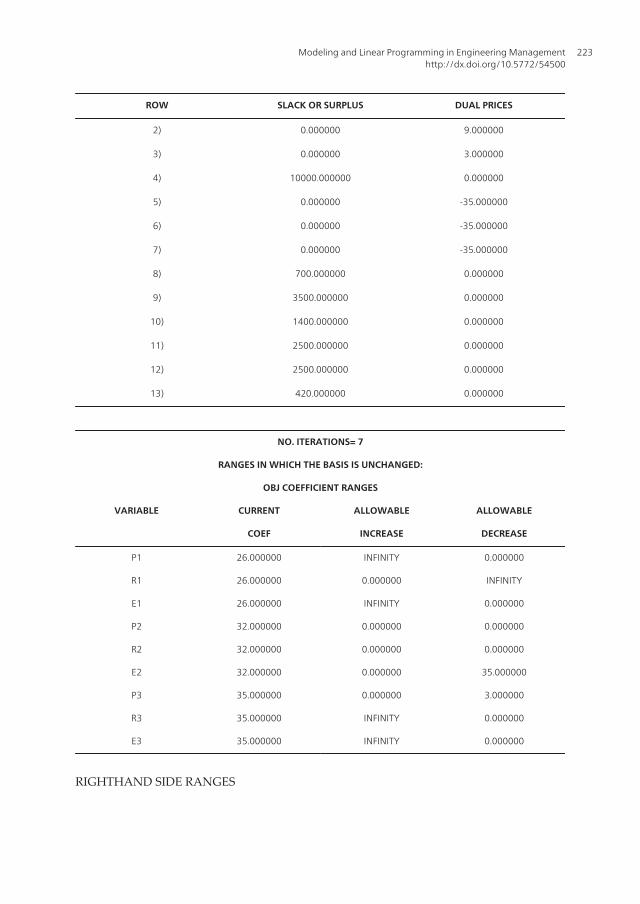
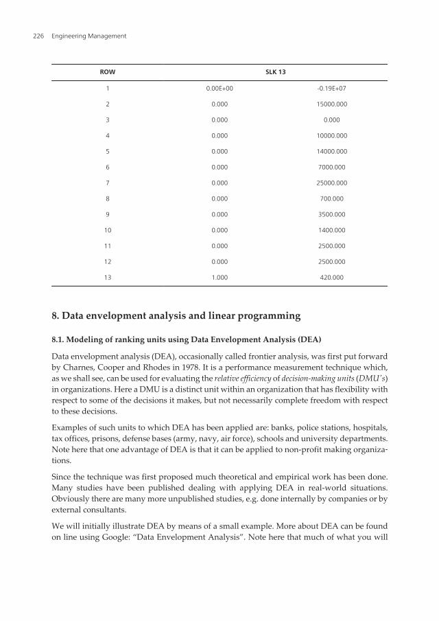
We present one of the solutions below with LINDO.
LP OPTIMUM FOUND AT STEP 7
OBJECTIVE FUNCTION VALUE
1) 1904000.
VARIABLE VALUE REDUCED COST
P1 0.000000 0.000000
R1 15000.000000 0.000000
E1 0.000000 0.000000
P2 0.000000 0.000000
R2 7000.000000 0.000000
E2 25000.000000 0.000000
P3 14000.000000 0.000000
R3 0.000000 0.000000
E3 0.000000 0.000000
Engineering Management218

ROW SLACK OR SURPLUS DUAL PRICES
2) 0.000000 9.000000
3) 0.000000 3.000000
4) 10000.000000 0.000000
5) 0.000000 -35.000000
6) 0.000000 -35.000000
7) 0.000000 -35.000000
8) 700.000000 0.000000
9) 3500.000000 0.000000
10) 1400.000000 0.000000
11) 2500.000000 0.000000
12) 2500.000000 0.000000
13) 420.000000 0.000000
NO. ITERATIONS= 7
RANGES IN WHICH THE BASIS IS UNCHANGED:
OBJ COEFFICIENT RANGES
VARIABLE CURRENT ALLOWABLE ALLOWABLE
COEF INCREASE DECREASE
P1 26.000000 INFINITY 0.000000
R1 26.000000 0.000000 INFINITY
E1 26.000000 INFINITY 0.000000
P2 32.000000 0.000000 0.000000
R2 32.000000 0.000000 0.000000
E2 32.000000 0.000000 35.000000
P3 35.000000 0.000000 3.000000
R3 35.000000 INFINITY 0.000000
E3 35.000000 INFINITY 0.000000
Modeling and Linear Programming in Engineering Managementhttp://dx.doi.org/10.5772/54500
219

RIGHTHAND SIDE RANGES
ROW CURRENT ALLOWABLE ALLOWABLE
RHS INCREASE DECREASE
2 15000.000000 4200.000000 0.000000
3 32000.000000 4200.000000 0.000000
4 24000.000000 INFINITY 10000.000000
5 14000.000000 10000.000000 14000.000000
6 22000.000000 0.000000 4200.000000
7 25000.000000 0.000000 4200.000000
8 0.000000 700.000000 INFINITY
9 0.000000 3500.000000 INFINITY
10 0.000000 INFINITY 1400.000000
11 0.000000 2500.000000 INFINITY
12 0.000000 INFINITY 2500.000000
13 0.000000 INFINITY 420.000000
THE TABLEAU
ROW (BASIS) P1 R1 E1 P2 R2 E2
1 ART 0.000 0.000 0.000 0.000 0.000 0.000
2 R1 1.000 1.000 1.000 0.000 0.000 0.000
3 P2 1.000 0.000 0.000 1.000 0.000 0.000
4 SLK 4 0.000 0.000 0.000 0.000 0.000
5 P3 0.000 0.000 0.000 0.000 0.000 0.000
6 R2 -1.000 0.000 -1.000 0.000 1.000 0.000
7 E2 0.000 0.000 1.000 0.000 0.000 1.000
8 SLK 8 0.150 0.000 0.000 0.000 0.000
9 SLK 9 -0.500 0.000 -0.500 0.000 0.000
10 SLK 10 -0.200 0.000 -0.200 0.000 0.000
11 SLK 11 0.000 0.000 0.150 0.000 0.000
12 SLK 12 0.000 0.000 0.200 0.000 0.000
13 SLK 13 -0.050 0.000 0.000 0.000 0.000
Engineering Management220

ROW P3 R3 E3 SLK 2 SLK 3 SLK 4 SLK 5
1 0.000 0.000 0.000 9.000 3.000 0.000 35.000
2 0.000 0.000 0.000 1.000 0.000 0.000 0.000
3 0.000 -1.000 -1.000 1.000 1.000 0.000 0.000
4 0.000 0.000 0.000 1.000 1.000 1.000 1.000
5 1.000 1.000 1.000 -1.000 -1.000 0.000 -1.000
6 0.000 1.000 0.000 -1.000 0.000 0.000 0.000
7 0.000 0.000 1.000 0.000 0.000 0.000 0.000
8 0.000 0.100 0.100 -0.100 -0.100 0.000 -0.050
9 0.000 1.000 0.000 -0.500 0.000 0.000 0.000
10 0.000 0.000 0.000 -0.200 0.000 0.000 0.000
11 0.000 0.000 -0.100 0.000 0.000 0.000 0.000
12 0.000 0.000 0.000 0.000 0.000 0.000 0.000
13 0.000 0.100 0.100 -0.100 -0.100 0.000 -0.030
ROW SLK 6 SLK 7 SLK 8 SLK 9 SLK 10 SLK 11 SLK 12
1 35.000 35.000 0.000 0.000 0.000 0.000 0.000
2 0.000 0.000 0.000 0.000 0.000 0.000 0.000
3 1.000 1.000 0.000 0.000 0.000 0.000 0.000
4 1.000 1.000 0.000 0.000 0.000 0.000 0.000
5 -1.000 -1.000 0.000 0.000 0.000 0.000 0.000
6 -1.000 0.000 0.000 0.000 0.000 0.000 0.000
7 0.000 -1.000 0.000 0.000 0.000 0.000 0.000
8 -0.100 -0.100 1.000 0.000 0.000 0.000 0.000
9 -0.500 0.000 0.000 1.000 0.000 0.000 0.000
10 -0.200 0.000 0.000 0.000 1.000 0.000 0.000
11 0.000 -0.100 0.000 0.000 0.000 1.000 0.000
12 0.000 -0.100 0.000 0.000 0.000 0.000 1.000
13 -0.100 -0.100 0.000 0.000 0.000 0.000 0.000
Modeling and Linear Programming in Engineering Managementhttp://dx.doi.org/10.5772/54500
221

ROW SLK 13
1 0.00E+00 -0.19E+07
2 0.000 15000.000
3 0.000 0.000
4 0.000 10000.000
5 0.000 14000.000
6 0.000 7000.000
7 0.000 25000.000
8 0.000 700.000
9 0.000 3500.000
10 0.000 1400.000
11 0.000 2500.000
12 0.000 2500.000
13 1.000 420.000
LP OPTIMUM FOUND AT STEP 7
OBJECTIVE FUNCTION VALUE
1) 1904000.
VARIABLE VALUE REDUCED COST
P1 0.000000 0.000000
R1 15000.000000 0.000000
E1 0.000000 0.000000
P2 0.000000 0.000000
R2 7000.000000 0.000000
E2 25000.000000 0.000000
P3 14000.000000 0.000000
R3 0.000000 0.000000
E3 0.000000 0.000000
Engineering Management222
ROW SLACK OR SURPLUS DUAL PRICES
2) 0.000000 9.000000
3) 0.000000 3.000000
4) 10000.000000 0.000000
5) 0.000000 -35.000000
6) 0.000000 -35.000000
7) 0.000000 -35.000000
8) 700.000000 0.000000
9) 3500.000000 0.000000
10) 1400.000000 0.000000
11) 2500.000000 0.000000
12) 2500.000000 0.000000
13) 420.000000 0.000000
NO. ITERATIONS= 7
RANGES IN WHICH THE BASIS IS UNCHANGED:
OBJ COEFFICIENT RANGES
VARIABLE CURRENT ALLOWABLE ALLOWABLE
COEF INCREASE DECREASE
P1 26.000000 INFINITY 0.000000
R1 26.000000 0.000000 INFINITY
E1 26.000000 INFINITY 0.000000
P2 32.000000 0.000000 0.000000
R2 32.000000 0.000000 0.000000
E2 32.000000 0.000000 35.000000
P3 35.000000 0.000000 3.000000
R3 35.000000 INFINITY 0.000000
E3 35.000000 INFINITY 0.000000
RIGHTHAND SIDE RANGES
Modeling and Linear Programming in Engineering Managementhttp://dx.doi.org/10.5772/54500
223

ROW CURRENT ALLOWABLE ALLOWABLE
RHS INCREASE DECREASE
2 15000.000000 4200.000000 0.000000
3 32000.000000 4200.000000 0.000000
4 24000.000000 INFINITY 10000.000000
5 14000.000000 10000.000000 14000.000000
6 22000.000000 0.000000 4200.000000
7 25000.000000 0.000000 4200.000000
8 0.000000 700.000000 INFINITY
9 0.000000 3500.000000 INFINITY
10 0.000000 INFINITY 1400.000000
11 0.000000 2500.000000 INFINITY
12 0.000000 INFINITY 2500.000000
13 0.000000 INFINITY 420.000000
THE TABLEAU
ROW (BASIS) P1 R1 E1 P2 R2 E2
1 ART 0.000 0.000 0.000 0.000 0.000 0.000
2 R1 1.000 1.000 1.000 0.000 0.000 0.000
3 P2 1.000 0.000 0.000 1.000 0.000 0.000
4 SLK 4 0.000 0.000 0.000 0.000 0.000
5 P3 0.000 0.000 0.000 0.000 0.000 0.000
6 R2 -1.000 0.000 -1.000 0.000 1.000 0.000
7 E2 0.000 0.000 1.000 0.000 0.000 1.000
8 SLK 8 0.1500.000
0.0000.000 0.000
9 SLK 9 -0.500 0.000 -0.500 0.000 0.000
10 SLK 10 -0.200 0.000 -0.200 0.000 0.000
11 SLK 11 0.000 0.000 0.150 0.000 0.000
12 SLK 12 0.000 0.000 0.200 0.000 0.000
13 SLK 13 -0.050 0.000 0.000 0.000 0.000
Engineering Management224

ROW P3 R3 E3 SLK 2 SLK 3 SLK 4 SLK 5
1 0.000 0.000 0.000 9.000 3.000 0.000 35.000
2 0.000 0.000 0.000 1.000 0.000 0.000 0.000
3 0.000 -1.000 -1.000 1.000 1.000 0.000 0.000
4 0.000 0.000 0.000 1.000 1.000 1.000 1.000
5 1.000 1.000 1.000 -1.000 -1.000 0.000 -1.000
6 0.000 1.000 0.000 -1.000 0.000 0.000 0.000
7 0.000 0.000 1.000 0.000 0.000 0.000 0.000
8 0.000 0.100 0.100 -0.100 -0.100 0.000 -0.050
9 0.000 1.000 0.000 -0.500 0.000 0.000 0.000
10 0.000 0.000 0.000 -0.200 0.000 0.000 0.000
11 0.000 0.000 -0.100 0.000 0.000 0.000 0.000
12 0.000 0.000 0.000 0.000 0.000 0.000 0.000
13 0.000 0.100 0.100 -0.100 -0.100 0.000 -0.030
ROW SLK 6 SLK 7 SLK 8 SLK 9 SLK 10 SLK 11 SLK 12
1 35.000 35.000 0.000 0.000 0.000 0.000 0.000
2 0.000 0.000 0.000 0.000 0.000 0.000 0.000
3 1.000 1.000 0.000 0.000 0.000 0.000 0.000
4 1.000 1.000 0.000 0.000 0.000 0.000 0.000
5 -1.000 -1.000 0.000 0.000 0.000 0.000 0.000
6 -1.000 0.000 0.000 0.000 0.000 0.000 0.000
7 0.000 -1.000 0.000 0.000 0.000 0.000 0.000
8 -0.100 -0.100 1.000 0.000 0.000 0.000 0.000
9 -0.500 0.000 0.000 1.000 0.000 0.000 0.000
10 -0.200 0.000 0.000 0.000 1.000 0.000 0.000
11 0.000 -0.100 0.000 0.000 0.000 1.000 0.000
12 0.000 -0.100 0.000 0.000 0.000 0.000 1.000
13 -0.100 -0.100 0.000 0.000 0.000 0.000 0.000
Modeling and Linear Programming in Engineering Managementhttp://dx.doi.org/10.5772/54500
225
ROW SLK 13
1 0.00E+00 -0.19E+07
2 0.000 15000.000
3 0.000 0.000
4 0.000 10000.000
5 0.000 14000.000
6 0.000 7000.000
7 0.000 25000.000
8 0.000 700.000
9 0.000 3500.000
10 0.000 1400.000
11 0.000 2500.000
12 0.000 2500.000
13 1.000 420.000
8. Data envelopment analysis and linear programming
8.1. Modeling of ranking units using Data Envelopment Analysis (DEA)
Data envelopment analysis (DEA), occasionally called frontier analysis, was first put forwardby Charnes, Cooper and Rhodes in 1978. It is a performance measurement technique which,as we shall see, can be used for evaluating the relative efficiency of decision-making units (DMU's)in organizations. Here a DMU is a distinct unit within an organization that has flexibility withrespect to some of the decisions it makes, but not necessarily complete freedom with respectto these decisions.
Examples of such units to which DEA has been applied are: banks, police stations, hospitals,tax offices, prisons, defense bases (army, navy, air force), schools and university departments.Note here that one advantage of DEA is that it can be applied to non-profit making organiza‐tions.
Since the technique was first proposed much theoretical and empirical work has been done.Many studies have been published dealing with applying DEA in real-world situations.Obviously there are many more unpublished studies, e.g. done internally by companies or byexternal consultants.
We will initially illustrate DEA by means of a small example. More about DEA can be foundon line using Google: “Data Envelopment Analysis”. Note here that much of what you will
Engineering Management226

see below is a graphical (pictorial) approach to DEA. This is very useful if you are attemptingto explain DEA to those less technically qualified (such as many you might meet in the militaryor management world). There is a mathematical approach to DEA that can be adoptedhowever. We will present the single measure first to demonstrate the idea and then move tomultiple measures and use linear programming methodology from our course.
Example 1. Ranking Banks
Consider a number of bank branches. For each branch we have a single output measure(number of personal transactions completed) and a single input measure (number of staff).
The data we have is as follows:
Branch Personal transactions ('000s) Number of staff
Branch 1 125 18
Branch 2 44 16
Branch 3 80 17
Branch 4 23 11
For example, for the Branch 2 in one year, there were 44,000 transactions relating to personalaccounts and 16 staff members were employed.
How then can we compare these branches and measure their performance using this data?
Ratios
A commonly used method is ratios. Typically we take some output measure and divide it bysome input measure. Note the terminology here, we view branches as taking inputs andconverting them (with varying degrees of efficiency, as we shall see below) into outputs.
For our bank branch example we have a single input measure, the number of staff, and a singleoutput measure, the number of personal transactions. Hence we have:
Branch Personal transactions per staff member ('000s)
Branch 1 6.94
Branch 2 2.75
Branch 3 4.71
Branch 4 2.09
Here we can see that Branch1 has the highest ratio of personal transactions per staff member,whereas Branch 4 has the lowest ratio of personal transactions per staff member.
Modeling and Linear Programming in Engineering Managementhttp://dx.doi.org/10.5772/54500
227

As Branch 1 has the highest ratio of 6.94 we can compare all other branches to it and calculatetheir relative efficiency with respect to Branch 1. To do this we divide the ratio for any branchby 6.94 (the value for Croydon) and multiply by 100 to convert to a percentage. This gives:
Branch Relative efficiency
Branch 1 100(6.94/6.94) = 100%
Branch 2 100(2.75/6.94) = 40%
Branch 3 100(4.71/6.94) = 68%
Branch 4 100(2.09/6.94) = 30%
The other branches do not compare well with Branch 1, so are presumably performing lesswell. That is, they are relatively less efficient at using their given input resource (staff members)to produce output (number of personal transactions).
We could, if we wish, use this comparison with Branch 1 to set targets for the other branches.
For example we could set a target for Branch 4 of continuing to process the same level of outputbut with one less member of staff. This is an example of an input target as it deals with an inputmeasure.
An example of an output target would be for Branch 4 to increase the number of personaltransactions by 10% (e.g. by obtaining new accounts).
Plainly, in practice, we might well set a branch a mix of input and output targets which wewant it to achieve. We can use linear programming.
8.2. Linear Programming example of DEA
Example 2. Ranking banks with linear programming
Typically we have more than one input and one output. For the bank branch example supposenow that we have two output measures (number of personal transactions completed andnumber of business transactions completed) and the same single input measure (number ofstaff) as before.
The data we have is as follows:
Branch
Personal
transactions
('000s)
Business
transactions
('000s)
Number of
staff
Branch 1 125 50 18
Branch 2 44 20 16
Branch 3 80 55 17
Branch 4 23 12 11
Engineering Management228

We start be scaling (via ratios) the inputs and outputs to reflect the ratio of 1 unit.
BranchPersonal transactions
('000s)
Business transactions
('000s)Per employee or staff
Branch 1 125/18=6.94 50/18=2.78 18/18=1
Branch 2 44/16=2.75 20/16=1.25 16/16=1
Branch 3 80/17=4.71 55/17=3.24 17/17=1
Branch 4 23/11=2.09 12/11=1.09 11/11=1
Pick a DMU to maximize: E1, E2, E3, or E4
Let W1 and W2 be the personal and business transactions at branch
In this example we choose to maximize branch two, E2.
Here is the LP formulation for this DEA problem:
Maximize E2
Subject to
E1 = 6.94 W 1 + 2.78 W 2E2 = 2.75 W 1 + 1.25 W 2E3 = 4.71 W 1 + 3.24 W 2E4 = 2.09 W 1 + 1.09 W 2E1≤1E2≤1E3≤1E4≤1
Now, what did we learn from this. If we ranked ordered the branches on efficiency perform‐ance of our inputs and outputs, we find
Branch 1 100%
Branch 3 100%
Branch 2 43.2%
Branch 4 36.2%
Modeling and Linear Programming in Engineering Managementhttp://dx.doi.org/10.5772/54500
229
We know we need to improve on branch 2 and branch 4 performances while not losing ourefficiency in branches 1 and 3. A better interpretation could be that the practices and proceduresused by the other branches were to be adopted by Branch 4, they could improve their per‐formance.
This invokes issues of highlighting and disseminating examples of best practices. Equally thereare issues relating to identification of poor practices.
In DEA the concept of the reference set can be used to identify best performing branches withwhich to compare poorly performing branches. If you use this procedure, use it wisely.
Author details
William P. Fox1 and Fausto P. Garcia2
1 Naval Postgraduate School, USA
2 Universidad Castilla-La Mancha, Spain
References
[1] Apaiah, R. & E. Hendrix ((2006). Linear programming for supply chain design: Acase on Novel protein foods. Ph.D. Thesis, Wageningen University, Netherlands.
[2] Balakrishnan, N. B, & Render, R. Stair. ((2007). Managerial Decision Making, 2nd Ed.Saddle River, NJ: Prentice Hall.
[3] Bazarra Mokhtar S. J.J. Jarvis, and H. D. SheralliLinear Programming and NetworkFlows, New York. John Wiley & Sons, (1990).
[4] EckerJoseph and M. Kupperschmid, Introduction to Operations Research, John Wi‐ley and Sons, (1988).
[5] Fox, W. P. (2012). Mathematical Modeling with Maple. Boston, MA: Cengage Pub‐lishers.
[6] Giordano, F, Fox, W, Horton, S, & Weir, M. (2009). A First Course in MathematicalModeling, 4th Ed. Belmont, CA: Brooks-Cole.
[7] Hiller Fredrick S and Gerald J. LibermanIntroduction to Mathematical Programming,McGraw Hill Publishing Company, (1990).
[8] Winston Wayne L. Introduction to Mathematical Programming Applications and Al‐gorithms, 4th Edition. Belmont, CA. Duxbury Press. (2002).
Engineering Management230


![[PPT]Table of Contents Chapter 2 (Linear Programming: …iuj.ac.jp/faculty/kucc625/policy/modeling/hillier/Chap... · Web viewTable of Contents Chapter 2 (Linear Programming: Basic](https://cdn.vdocuments.mx/doc/165x107/5adaf71c7f8b9ae1768de5a2/ppttable-of-contents-chapter-2-linear-programming-iujacjpfacultykucc625policymodelinghillierchapweb.jpg)