
Model Sensitivity, Performance
and Evaluation Techniques
for
The Air Pollution Model
in Southeast Queensland
Natalie Joanne Leishman
Bachelor of Applied Science
In partial fulfilment of the requirements for the degree of
Master of Applied Science
School of Natural Resource Sciences
2005


Keywords
Meteorology, TAPM, statistics, synoptic cluster type, modelling, performance, wind speed,
wind direction, temperature.
Abstract
One important component for successful air quality modelling is the utilisation of a
reliable meteorological simulator. Evaluating the model with respect to its overall
performance in predicting natural processes is no easy task. The problem is twofold,
firstly there is the availability and suitability of field data with which to compare a
model with and secondly there is the method of evaluation. The Air Pollution Model
(TAPM), developed by the CSIRO was used to simulate the winds in Southeast
Queensland (SEQ). The complex nature of the airshed makes it difficult to compare
modelled data with observational data as the observational data may be influenced by
local phenomena. Evaluation of the model through the use of standard statistics and
monthly and seasonal statistics illustrated that overall the model predicted the annual
average wind speeds and temperatures well. Through the use of synoptic clustering,
more detail on model performance was gained and it was found that TAPM predicted
sea breezes that occurred on high pollution days. The sensitivity of the model to the
selection of input parameters such as soil type, land use, vegetation, and rain
processes was also investigated.

TABLE OF CONTENTS
1. Introduction...........................................................................................................1
1.1 Prognostic modelling .................................................................................4
1.2 Method of evaluation .................................................................................5
1.3 The Southeast Queensland Airshed ...........................................................7
1.4 Previous work ............................................................................................8
2. TAPM .................................................................................................................11
3. Methodology for performance evaluation ..........................................................17
3.1 Statistical approaches...............................................................................17
3.2 Clustering .................................................................................................18
3.3 Meteorological data sets...........................................................................25
3.3.1 Surface characteristics .................................................................28
3.3.2 Likely boundary layer structure at each site ................................28
4. Model configuration............................................................................................31
5. Results.................................................................................................................33
5.1 One year of modelling: 1999 ...................................................................33
5.1.1 Mean wind speed and temperature ..............................................33
5.1.2 Diurnal profiles for temperature and wind speed ........................35
5.1.3 Wind direction .............................................................................40
5.1.4 Statistical analysis........................................................................49
5.2 Sensitivity analysis...................................................................................51
5.2.1 Soil moisture and rain ..................................................................51
5.2.2 Selection of roughness length ......................................................56
5.2.3 Sensitivity to soil type..................................................................59
5.2.4 Sensitivity to data assimilation ....................................................61
5.2.5 Sensitivity to grid resolution........................................................61
5.3 Performance of model based on cluster types..........................................62
5.3.1 Diurnal profiles of wind speed and temperature..........................64
5.3.2 Case day 30 January 1999............................................................67
5.3.3 Case day 5 March 1999................................................................70
5.3.4 Case day 21 June 1999.................................................................73
6. Discussion...........................................................................................................77
7. Conclusions.........................................................................................................81

8. References...........................................................................................................85
Appendix A: Meteorological component of TAPM
Appendix B: Statistical Formulae
Appendix C: Cluster definitions for cluster types
Appendix D: Summer and winter/autumn pollution conducive days

TABLES
Table 3.1: Meteorological parameters (3am and 9am) for Eagle Farm Airport
1952 - 2000...........................................................................................20
Table 3.2: Meteorological parameters (9am and 3pm) for Amberley Airport 1952
- 2000....................................................................................................22
Table 3.3: Cluster types most conducive to pollution events ................................23
Table 3.4: Cluster definitions for significant cluster types for pollution events ...24
Table 3.5: Description of monitoring stations .......................................................27
Table 3.6: Surface roughness and soil type characteristics for each monitoring
site. .......................................................................................................28
Table 5.1: Predicted and observed mean temperature...........................................34
Table 5.2: Predicted and observed mean wind speed (ms-1) .................................34
Table 5.3: Statistics for (a) temperature (oC), (b) wind speed, (c) wind speed
component u and (d) wind speed component v....................................50
Table 5.4: Statistics for (a) temperature (oC), (b) wind speed, (c) wind speed
component u and (d) wind speed component v, for Flinders View and
Rocklea, with and without rain processes. ...........................................52
Table 5.5: Predicted annual temperature and wind speed for various grid
resolutions at Flinders View.................................................................62
Table 5.6: Best (IOA>0.8) and worst (IOA<0.5) cluster types based on IOA based
on predictions of the model (wspd and wdir).......................................63

FIGURES
Figure 1.1: Modelling domain including Local Government Authorities and
selected monitoring stations used in this study ......................................7
Figure 3.1: Location of monitoring sites used for model validation ......................26
Figure 4.1: Classification of vegetation types for Southeast Queensland ..............31
Figure 4.2: Classification of soil types for Southeast Queensland .........................32
Figure 5.1: Hourly profile of predicted and observed mean wind speed for
Deception Bay ......................................................................................37
Figure 5.2: Hourly profile of predicted and observed mean temperature and wind
speed for Eagle Farm............................................................................37
Figure 5.3: Hourly profile of predicted and observed mean temperature wind speed
for Rocklea ...........................................................................................38
Figure 5.4: Hourly profile of predicted and observed mean temperature and wind
speed for Flinders View .......................................................................38
Figure 5.5: Hourly profile of predicted and observed mean temperature and wind
speed for Moreton Island......................................................................39
Figure 5.6: Distribution of wind direction for predicted and observed at Deception
Bay for (a) summer, (b) autumn, (c) winter and (d) spring..................41
Figure 5.7: Distribution of wind direction for predicted and observed at Eagle
Farm for (a) summer, (b) autumn, (c) winter and (d) spring................42
Figure 5.8: Distribution of wind direction for predicted and observed at Rocklea
for (a) summer, (b) autumn, (c) winter and (d) spring .........................43
Figure 5.9: Distribution of wind direction for predicted and observed at Flinders
View for (a) summer, (b) autumn, (c) winter and (d) spring................44
Figure 5.10: Distribution of wind direction for predicted and observed at Moreton
Island for (a) summer, (b) autumn, (c) winter and (d) spring ..............45
Figure 5.11: Wind speed versus wind direction for Deception Bay (a) observations
(b) predictions ......................................................................................47

Figure 5.12: Wind speed versus wind direction for Eagle Farm (a) observations (b)
predictions ............................................................................................47
Figure 5.13: Wind speed versus wind direction for Rocklea (a) observations (b)
predictions ............................................................................................48
Figure 5.14: Wind speed versus wind direction for Flinders View (a) observations
(b) predictions ......................................................................................48
Figure 5.15: Comparison of observed temperature with predicted temperature (with
and without rain and change in soil moisture) for Rocklea..................54
Figure 5.16: Comparison of observed wind speed with predicted wind speed (with
and without rain and change in soil moisture) for Rocklea..................54
Figure 5.17: Comparison of observed temperature with predicted temperature (with
and without rain and change in soil moisture) for Flinders View........55
Figure 5.18: Comparison of observed wind speed with predicted wind speed (with
and without rain and change in soil moisture) for Flinders View........55
Figure 5.19: Timeseries of temperature and wind speed at Flinders View ..............57
Figure 5.20: Timeseries of (a) evaporative heat flux and (b) sensible heat flux at
Flinders View for vegetation of grassland and vegetation of urban.....58
Figure 5.21: Timeseries of (a) temperature, (b) wind speed, (c) evaporative heat
flux and (d) sensible heat flux for sandy clay loam soil and clay soil .59
Figure 5.22: Predicted wind speed at Flinders View for the 1 km, 3 km and 6 km
resolution grids. ....................................................................................62
Figure 5.23: Box and whisker plot of IOA for each cluster type for wind speed each
site. .......................................................................................................63
Figure 5.24: Wind speed difference profiles for Deception Bay (a) summer and (b)
winter pollution conducive days ..........................................................66
Figure 5.25: Temperature difference profiles for Flinders View (a) summer and (b)
winter pollution conducive days ..........................................................66
Figure 5.26: Timeseries plots of wind direction and wind speed for (a) Deception
Bay, (b) Eagle Farm, (c) Rocklea and (d) Flinders View, 30 January
1999, ozone pollution conducive day...................................................68

Figure 5.27: Timeseries plots of wind direction and wind speed for (a) Deception
Bay, (b) Eagle Farm, (c) Rocklea and (d) Flinders View, 5 March 1999,
ozone pollution conducive day.............................................................71
Figure 5.28: Timeseries plots of wind direction and wind speed for (a) Deception
Bay, (b) Eagle Farm, (c) Rocklea and (d) Flinders View, 21 June 1999,
NOx pollution conducive day ...............................................................74

Statement of original authorship
The work contained in this thesis has not been previously submitted for a degree or
diploma at any other higher education institution. To the best of my knowledge and
belief, the thesis contains no material previously published or written by another
person except where due reference is made.
Signed: _____
Date:

Acknowledgements
I could not have written this thesis without the support of many people. I would like to
thank the Queensland University of Technology for their support of me as a
postgraduate student. To my supervisor Neville Bofinger, thank you for your belief in
me when I turned up unannounced at your door, your guidance and inspiration. For all
your quotes, my life is richer. Thank you to my co-supervisor Aaron Wiegand, for
helping me with the fundamentals. To Mum, this is for you, for your continuing
support and encouragement. And Nana may you look upon me wherever you may be
and know that without your love of science and maths, I may never have known the
wonders. And to my friends, it’s been a long time, but here it is.

1
1. Introduction
The accuracy of an air quality simulation model relies upon the assumptions made
about physical and chemical processes in the atmosphere involving the transport and
transformation of pollutants, as well as the quality of meteorological information and
simulation scheme and emissions data (Elbir, 2003).
One important component for successful air quality modelling is the utilisation of a
reliable meteorological simulator. There are various models in circulation, each with
its own set of algorithms in place to simulate the real life meteorological processes.
The uptake of these models is varied. Difficulties in obtaining detailed site-specific
data on temporal and spatial scales for a region of interest have seen prognostic
models being used more readily.
The Air Pollution Model, TAPM (Hurley, 2001) is one such model. TAPM is the next
stage in modelling in Australia on from the Lagrangian Atmospheric Dispersion
Model developed by CSIRO which involved intensive computer modelling on a
supercomputer and detailed meteorological information. TAPM can be used for
pollution modelling, but its main benefit is that it can be used as a meteorological
preprocessor for other models that require site-specific data in order to carry out air
pollution modelling.
For a minimal cost TAPM can be purchased along with default databases for terrain,
soil type, land use and vegetation. This enables the user to execute the model without
the necessity to assemble large data sets from external sources, and requiring the
selection of only a limited number of adjustable parameters. But how sensitive is the
model to these selections? Makar et al (2005) discovered that, for weather forecasting,
while surface roughness alone did not have a significant effect on temperature and
wind speeds, heat flux did.
This thesis investigates the effects of changes in the selection of soil type, vegetation
and land use and deep soil moisture content and the subsequent changes in surface
roughness and heat fluxes. While this work does not resolve whether the physical

2
processes within the model algorithms adequately represent the natural processes
(recommended for future work), it identifies which of these areas the user must
carefully prescribe and where possible incorporate additional observational data
within the modelling.
Evaluating the model with respect to its overall performance in predicting natural
processes is no easy task. The problem is twofold, firstly there is the availability and
suitability of field data with which to compare a model and secondly there is the
method of evaluation.
In this study, the performance of TAPM is evaluated in the Southeast Queensland
airshed. Southeast Queensland is situated approximately at latitude 28 oS and
longitude 153.9 oE and has a subtropical climate influenced to some extent by its
position on the eastern coastline. The well-vegetated mountain ranges to the north and
west near the coast make Southeast Queensland naturally susceptible to spatially
complex wind and recirculation patterns. Southeast Queensland consists of rural and
sub-rural areas as well as a large populated and industrial metropolitan area
(Brisbane) which is located at the centre of the airshed resulting in anthropogenic heat
fluxes contributing to the already complex nature of the airshed.
Southeast Queensland has an established and extensive meteorological and air quality
monitoring network with monitoring stations spread across the region recording the
standard meteorological parameters of wind speed, wind direction and temperature.
Due to the complexity of the region, each monitoring station tends to represent its
own unique local air system.
The five monitoring stations selected for this work represent quite different locations
within the airshed. The performance of the model in predicting the surface
characteristics of wind speed, wind direction and temperature at these sites will be
investigated with regard to the suitability of each site and to whether direct
comparison between modelled and observed information is appropriate.
The application of TAPM to the Southeast Queensland airshed will provide
significant insight into the prevailing meteorological conditions and the

3
photochemistry in the airshed. Use of the model will assist in the understanding of
the processes in the airshed, thus becoming a management tool for policy and
legislation implementation on air quality for Queensland.
There are no set guidelines for correctly evaluating a mesoscale meteorological
model. The German Association of Engineers, VDI, has been working on an
evaluation guideline to evaluate the performance of a single model and to compare the
performance of different models (Schlünzen et al, 2004). ASTM (2000) in providing
guidance for air quality modelling suggests, “There has also been a consensus
reached on the philosophical reasons that models of earth science processes can
never be validated, in the sense that a model is truthfully representing natural
processe.” While this may be the case, understanding the performance of the model
and the areas in which it may perform well, and those instances where it may not, are
important.
Standard statistical techniques, such as the mean and standard deviation can be used,
along with Index of Agreement (Willmott, 1981), fractional bias and investigating the
percentage of modelled results in an allowable range determined by the quality of the
observational data (Schlünzen, 2004). However, these statistics over the entire
simulation database alone are incapable of discriminating between differences in
model performance. In this thesis, the model performance will be evaluated over
particular subsets of synoptic day type as well as detailed investigation of seasonal
and diurnal components.
Wind field studies for the Southeast Queensland airshed have been conducted for the
last fifteen years. The Coffey (1993) study (involving Katestone Scientific and
CSIRO) and Ischtwan and Cope (1996) have focused on reproducing windfields for
specific days, representative of high pollution events and recirculation (which is of
particular importance for winter time pollution events). In this thesis further
evaluation of a newer model will be undertaken by using synoptic cluster types to
categorise those days with conditions conducive to pollution events and the model’s
performance evaluated.

4
The objectives of this thesis are to:
• Evaluate the performance of TAPM in simulating key day types identified as
being important for high pollution events for the Southeast Queensland airshed.
• Determine a method for model evaluation that will allow reasonable
assessment of the model performance, taking into consideration the quality and
appropriateness of observational data, statistical measures and synoptic
clustering that can be used to elicit detailed information on model performance.
• Understand the sensitivity of the model with respect to selection of user-
defined parameters to maximise model performance.
1.1 Prognostic modelling
One important component for successful air quality modelling is the utilisation of a
reliable meteorological simulator. Prognostic meteorological modelling (which
includes full numerical solutions of mass, energy and momentum conservation
equations) removes the need to have site-specific data to be input into the model other
than basic synoptic data, eliminating the cost and time associated with compiling a
comprehensive data set for inclusion into a model. However, reproducing reality with
a reasonable degree of accuracy is more difficult than simply executing a model and
extracting the meteorological results. There are many questions such as:
• How to adequately represent surface flows when using synoptic scale
information as the base information?
• Is the resolution of the model adequate to simulate the surface roughness and
therefore reproduce the flows close to the surface?
• Does the model represent and differentiate between the air flows in the urban
areas and the air flows in the rural areas? This is important in transition areas
(e.g. at the outskirts of an urban area where wind flows may have either quasi-
urban or quasi-rural characteristics, depending on wind direction) and in the
interior of cities, forests or ranges of hills where the roughness elements give
rise to a surface roughness layer of considerable vertical extent.

5
• How to set the lower boundary conditions through selection of soil moisture
(the only tunable parameter in TAPM once landuse is chosen) to correctly
determine the heat fluxes occurring and subsequent temperature differences at
the surface?
• How to resolve sharp gradients in temperature and wind speed which may be
induced as a result of sea and land interfaces?
Once the modelling has been completed, a comprehensive evaluation of model
performance is required.
1.2 Method of evaluation
There is no agreed scheme for evaluating mesoscale meteorological models. The
most simplistic method is to use graphical analysis such as scatter plots, timeseries
comparisons and cumulative plots of predicted and observed parameters at a given
location. This allows for obvious differences in data to be detected immediately.
Basic statistics as recommended by Skjøth (2005), such as the mean, standard
deviation, correlation, bias and root mean square error of the observed and predicted
data sets also give insight into the predictive capability of the model, such as whether
the observations and predictions are linearly independent, whether the variance within
the two data sets is similar and whether the model is underpredicting or
overpredicting.
The utility of windfield simulations is usually judged by various measures that look at
overall correlation structure, indices of agreement (IOA) or biases at a given location
for a time period. Various studies show the IOA to be a good measure in assessing
the general predictive capabilities of a model but it can be limiting as it is only
assessing a given location for a particular time period.
Such overall measures may be less useful in determining whether the critical features
of the near-surface met fields are well described for a given application (e.g. if a
model predicts the mean to be twice the measured mean, the correlation could still be
high. Meanwhile the IOA reflects the absolute difference between observations and
predictions, rather than the relative differences between the observations and the
predictions. This may result in significant differences in one parameter for one hour to
be lost.).The IOA and simple measures give little information on the reproducibility

6
of the spatial correlations in the meteorological fields or whether the regular cycles
such as diurnal and synoptic periodicities are well represented by the model. A
detailed investigation of seasonal, weekly and diurnal components is also
advantageous to see how well the model does at various time resolutions (Rao et al,
1999).
The use of monitoring information to generate a synoptic classification of days allows
the results of the modelling to be divided into distinct and useful categories for a more
detailed analysis (for example, days where an afternoon sea breeze is evident). The
above-mentioned performance measures can then be reviewed based on these
synoptic day types.
All methods of performance evaluation have advantages and disadvantages but all
rely on the use of unfiltered or adjusted observational data and in some cases it is the
quality and limited generality of the observational data that governs the quality of the
validation. If too much faith is put in to the measurements at these monitoring
stations, it is possible to expect too much from a model if you expect the model to
predict the observed data exactly.
Further detailed performance analysis can be conducted looking at:
• Multiscaling techniques to downscale or upscale between point measurements
and model predictions at various resolutions to eliminate the error of
“representativeness” that arises when comparing data from different sources
(Tustison et al, 2003).
• Performance measures based on the information content for the application at
hand. An example of this is the fractional bias between any predicted and
observed parameter X, evaluated over different synoptic clusters and weighted
by hourly factors reflecting the user’s view of the importance of the hour in a
given application (Jackson et al, 2003).
• Defining the percentage of model results within an allowable range (Schlünzen
et al, 2004). A hit is defined by the percentage of model results within an
allowable range (D) set based on the measured data. D also accounts for the
likely accuracy of the measurements themselves. If wind speed measurements

7
were accurate to +/- 0.5 ms-1 than if the model predictions were within this
range, it would be counted as a hit.
1.3 The Southeast Queensland Airshed
The Southeast Queensland airshed covers an area of about 57,600 km2, centred on
southeast of Brisbane and encompassing the eighteen local government areas between
the Gold and Sunshine Coasts, and from Toowoomba in the west to the Moreton Bay
Islands in the east. Most urban and associated development is located in the lowland
areas close to the coast. Half of this region is classed as urban and half as non-urban.
Although situated on relatively flat ground, Brisbane is a city surrounded by complex
terrain, with the D’Aguilar Range to the northwest, Flinders Peak to the southeast and
Tamborine Mountain to the south, all situated within 40km of the city and the Great
Dividing Range further a field to the southwest and northwest. To the east lies a
complex coastline, with several major islands within 20km of the city (refer to Figure
1-1 for map of Southeast Queensland).
Figure 1.1: Modelling domain including Local Government Authorities and selected monitoring stations used in this study

8
This orography is known to lead to complex wind patterns. The terrain, valleys and
the Brisbane River may add to the channelling of local winds or the subsequent
blocking of winds. Drainage flows (the flow of cooler air travelling down a slope as a
result of nocturnal cooling) impact on the airshed due to the range to the north and
south. Katestone Scientific (As part of Coffey, 1993) identified four main types of
drainage flow patterns as follows:
• "West to northwesterlies in the area to the west of Ipswich.
• West to southwesterlies in the Rocklea area (Rocklea is situated 6 km southwest
of the Brisbane CBD).
• Southwesterly winds in the north of Brisbane.
• South to south-southwesterly drainage flows near Beaudesert which
presumably re-inforce the northerly drift of pollutants in the general Brisbane
area in the early mornings".
The coastal siting of Brisbane and its sub-tropical climate result in the late morning
and afternoon winds being dominated by sea breezes (even on many days in winter
for the coastal strip). Depending on other factors within the airshed, the sea breeze can
penetrate as far inland as Dalby on the Darling Downs, some 200 km from the
Brisbane CBD.
This topography generates local wind flows that play an important role in dispersion
of air pollutants in the Southeast Queensland region (DOE, 1997) and therefore
accurate characterisation of the meteorology is essential for understanding the factors
that influence air quality in the region.
1.4 Previous work
Simpson and Auliciems (1989) highlighted that the topography of Southeast
Queensland was a strong influence in retaining pollutants in Brisbane under suitable
meteorological conditions.
Various studies have been conducted by Johnson (1992), CSIRO and Katestone
Scientific in conjunction with Coffey Partners (1993) that investigate the
meteorological conditions which are conducive to pollution events in Southeast
Queensland. Techniques such as clustering have been used to assist in determining

9
“like days” - days with similar synoptic conditions. From these studies three day
types that are conducive to smog events were defined from air quality and
meteorology at the three long-term sites to 1992. The recirculation of air within the
airshed gives rise to high pollution days, particularly when the pollution from the City
in the afternoon moves out to the southwest during the night, before passing back to
the City the next morning to combine with the fresh City emissions.
As classified by Johnson these day types were:
“Type 1: Clear morning southwesterly winds at Rocklea, with the photochemical
event occurring with the north-northeasterly sea breeze front. Smog
concentrations are likely to increase downwind from Rocklea in the
sea breeze.
Type 2: Recirculated smog from the previous day occurs during the morning at
Rocklea with the wind from the southwest. A second photochemical
event occurs later with a north-northeasterly sea breeze front similar
to type 1.
Type 3: A polluted air mass persists all day at Rocklea, at least. The morning
wind is from the northwest with a sea breeze in the afternoon. Many
multiday pollution events consist of this day type.”
Based on this work, the Environmental Protection Agency of Queensland (EPA)
modelled for the following days:
• January 15, 1987
• August 17, 1979
• September 22, 1986
• November 9, 1995
The simulation of these ozone events, which were the foundation of early studies and
reports of the Brisbane Airshed, are based on only two of the four available
windfields: January 15, 1987 and November 9, 1995 (DOE, 1997). These days were
modelled as they represented typical air flow for a summer and winter day.
These simulations were produced with the Lagrangian Atmospheric Dispersion Model
(LADM), developed by the Division of Atmospheric Research at Australia’s

10
Commonwealth Scientific and Industrial Research Organisation, CSIRO. This model
essentially solves the equations governing the behaviour of the atmosphere. LADM
was a key component of many major Australian air pollution studies including the
Metropolitan Air Quality Strategy for the New South Wales Environment Protection
Authority; and the design of the Brisbane air quality monitoring network design for
Queensland Environmental Protection Agency, Brisbane City Council and QEC.
(http://www.dar.csiro.au/ladm)
Continual improvements and development of CSIRO models has led to the
development of The Air Pollution Model (TAPM), a model which does not require
site-specific meteorological data as an input. Although TAPM has been verified for
regions in Australia and overseas such as Kwinana, Perth, Cape Grim (Tasmania), and
Mt Isa (Queensland), as well as Kuala Lumpur (http://www.dar.csiro.au/tapm/), the
validation of TAPM for the Southeast Queensland domain is yet to be documented.
The Queensland EPA and Brisbane City Council have advocated TAPM as the basis
for a regional air quality model.

11
2. TAPM
TAPM is a three dimensional prognostic model used to predict concentrations of
pollutants over a gridded domain. Configuration and execution of the model is
simplified with the inclusion of a graphical user interface (GUI). The GUI is also used
in the analysis of output data.
The model includes synoptic scale meteorology in conjunction with terrain which
induces airflows and sea breezes predicted by the fluid dynamics approach. This
minimises the need for detailed site-specific meteorological data. The mean
horizontal wind components are determined using the momentum equation and the
terrain-following vertical velocity is solved using the continuity equation. Weighted
averages of soil and vegetation values are used to calculate the surface temperature
and moisture. Relevant equations are included in Appendix A.
A nested grid approach is utilised. The size of the outer grid is best suited to less than
1000 km x 1000 km but recommended to be greater than 650 km x 650 km. This is to
make sure that the mesoscale effects are taken into account and the upper limit is due
to the model not accounting for the curvature of the earth.
Air pollution is modelled using predicted meteorology and turbulence from the
meteorology component.
TAPM is continually evolving from its early inception in 1997. An early validation of
the model was conducted in the Kwinana Coastal Fumigation Study performed by
Hurley and Luhar (2000). The model was extended to allow for nesting of the domain,
non-hydrostatic simulations and a vegetative canopy at the surface. The performance
of the model was investigated for four case studies. It was found that the model
generally captured the features of strong sea breeze circulation and that it modelled
the wind speed, wind direction and temperature parameters successfully. Wind speed
was generally within 1-2 ms-1 of that observed below 500 m, and wind direction
within10-20o of that observed.

12
Various model validation studies have been carried out for TAPM. The studies have
ranged from one day studies in which TAPM was validated by replication of an ozone
event such as by Azzi et al (2002). In this study the performance of the model to
predict the temperature and vertical structure was investigated and it was concluded
that further studies of ozone events were to be investigated to confirm the
performance of the model as there was differences in the predicted results and the
observed data.
The model has also been investigated for monthly periods characterised by high air
pollution concentrations and was found to predict near-surface meteorology well
(Hurley, 2000). The model has also been validated for one year simulations in
Melbourne (Hurley, 2000) and Pilbara Region (Physick et al, 2002) also validated the
model for one year simulations in Melbourne and Pilbara Region. In Melbourne the
model was used to confirm the accuracy of a recently developed emissions inventory.
The performance of the model under various conditions has also been investigated.
These have ranged from the urban and coastal dispersion of point sources, where the
model was applied to Indianapolis, USA and Kwinana, Australia (Luhar and Hurley
2002).
TAPM has also been used for air quality management. Graham and Bridgman (2002)
investigated the suitability of the model to be used as a modelling tool for the Lake
Macquarie Council. Ischtwan (2002 and unpublished) is investigating the suitability
of the model for summer ozone predictions in Southeast Queensland. In Gladstone,
Queensland the model has been used coupled with CALPUFF and used as an air
quality management tool (Killip et al, 2002).
In general, for the various studies mentioned as well as others such as Physick et al
(2002a), Physick et al (2002b), Luhar et al (2004), Hibberd et al (2003) and Jackson et
al (2003) the model has predicted the surface meteorology (wind speed, wind speed
vector components u and v and temperature) successfully when using annual statistics
for comparison. Jackson et al (2003) highlighted that for multiple sites around
Australia, the model consistently overpredicted the average wind speed. At 21 sites
(out of 26) the wind speed was overpredicted. Eight of these sites had the wind speed

13
overpredicted by more than 20 %. Further analysis of the location and height above
sea-level of each site failed to find a relationship between model performance and
each of the sites.
Physick et al (2002) and Luhar et al (2004) looked at sea breezes and other
phenomena that are characteristic wind patterns at coastal sites. Physick et al (2002)
investigated the ability of the model to adequately represent the thermal profiles that
are important in predicting fumigation and recirculation patterns that occurred at the
coastal site in Western Australia. Recirculation patterns have been documented
previously as an example of meteorological conditions that are significant in air
quality events in Southeast Queensland (Johnson, 1992 and Coffey, 1993). The
temperature profiles were predicted adequately by the model, and the statistical
analysis showed there was very good agreement, apart from the slight overprediction
of wind speeds, giving confidence that the dispersion modelling would adequately
represent plume dispersion of tall stacks in the area, whether the dispersion event be
fumigation or plume trapping above the mixing height. Luhar et al (2004)
investigated the effect that inclusion of data assimilation in the model had on
predicted winds. Comparison of observed winds and predicted winds (model run with
data assimilation) found that for the particular site a significant improvement was
made, with nearly perfect correlation between the observed and predicted data. The
winds at another site close by also improved with data assimilation included, however
not to the same extent.
Hibberd et al (2003) conducted a verification study of TAPM at multiple sites in
Western Australia. Once again, annual statistics were used to determine model
performance. This particular study found quite different results for model comparison
with the various monitoring stations. In general, the wind speed was overpredicted,
with wind speeds 31 – 105 % higher at some sites. It was thought that the location of
the monitoring sites close to trees and/or creeks may have contributed to the
differences in predicted and observed winds and therefore it was concluded that it was
not actually model performance but poor siting of the observational sites. The wind
speed at two monitoring sites that were located in paddocks was predicted well,
comparatively to the others. The domain studied was also heavily forested in areas,
not unlike Southeast Queensland. The author conducted landuse experiments by

14
changing the surface roughness from 1.0 m (typical of tall forests) to 0.3 m as the drag
along densely populated forest is expected to be less than for a less dense forest.
Changing the surface roughness resulted in a 15 % lowering of the predicted wind
speeds. The subsequent pollution modelling results showed the predicted
concentrations remained unchanged at some sites while a 14 % change was observed
at another, attributed to the change in wind speed due to the change in the surface
roughness. Further discussion of possible differences between the predicted and
observed wind speeds highlighted the difficulty in comparing the winds recorded at a
monitoring site (typically at 10 m elevation) and the winds predicted by the model (at
10 m above the zero-plane displacement). For areas of tall vegetation where heights of
trees may be 15 m this means TAPM 10 m winds are actually at a height of 22 m,
which naturally would result in higher wind speeds as the observed meteorology is
usually recorded at a height of 10 m. Which once again raises the issue of how to
eliminate the error of “representativeness” that arises when comparing data from
different sources.
As TAPM has evolved over the last few years, it has become an important tool for
meteorological and air quality simulation modelling in many Australian areas as it
does not need site specific data. TAPM is also being utilised as a source of
meteorological data for local pollution modelling investigations where there is a lack
of site representative measurements. TAPM meteorological data is commonly used
with regulatory models such as AUSPLUME (Lorimer, 1986) CALPUFF.
There are a few variables that the user can vary to improve the performance of the
model. For sensitivity analysis of TAPM the user can change
• The land use option, which governs the roughness length and roughness height;
• The deep soil moisture content which is used for the lower boundary condition
in the soil, however the evaporative and rain processes in the model determine
the soil moisture for each grid cell throughout the model run;
• Rain processes which can be switched on/off; and
• Whether the non-hydrostatic option is on or off.

15
To also improve the model predictions, data assimilation can be included (where data
are available) to nudge the model solution towards the observed surface wind speed
and direction at the site for which the data are included.
The inputs into TAPM are:
• Six-hourly synoptic data (LAPS) at 0.75 degree spacing;
• terrain height data;
• vegetation and soil type data;
• monthly mean sea surface temperatures; and
• soil moisture content.
Meteorological parameters output from the model include temperature, wind speed,
wind direction, relative humidity, net radiation, sensible heat flux and evaporative
heat flux, output as hourly averages for the run period at a particular location of
interest in the grid. Vertical profiles are also available for meteorological parameters
such as wind speed, wind direction, temperature, specific humidity of water vapour,
specific humidity of cloud water, turbulence kinetic energy and height above ground
at a particular location. These can be viewed as hourly averages or overall averages
for the entire run time. TAPM also allows output files to be extracted for input into
other models, such as AUSPLUME, CALMET and AERMOD.

16

17
3. Methodology for performance evaluation
Statistical methods provide a way of evaluating the model performance by comparing
the modelled data with observations from the field. Standard measures can provide an
overview of model performance. Synoptic classification can provide more detail as to
what day types TAPM may or may not predict well. Limitations to the evaluation can
arise from the quality and appropriateness of the observational data being used for the
comparison.
3.1 Statistical approaches
TAPM has been used to predict hourly average temperature and horizontal wind
components u and v at 10m above the ground (first model layer) at the nearest grid
point to each of the Qld EPA and Bureau of Meteorology monitoring stations in
Southeast Queensland. A statistical analysis has been undertaken using the
recommendations of Willmott (1981) to evaluate the performance of the model.
Statistics used included:
• Mean and standard deviation of the modelled and observed data;
• Root mean square error (rmse). Low rmse values in a model indicate that the
model is explaining most of the variation in the observations; and
• Systematic (rmse_s) and unsystematic (rmse_u) components. If the model is
unbiased, rmse_s should approach 0 and rmse_u should be close to rmse.
Measures of variational skill were also used. According to Pielke (1984) a model is
predicting with skill if:
(a) the standard deviations of the predictions and observations are approximately the
same. OstdPstdvskill =_ , skill_v should =1 where Pstd is the standard deviation of
the modelled data and Ostd is the standard deviation of the observed data.
(b) rmse is less than the standard deviation of the observations
Ostdrmserskill =_ , skill_r should be less than 1, ideally, where rmse is the root
mean square error and Ostd is the standard deviation of the observations.
18
The Index of Agreement (IOA) determines the degree to which magnitudes and signs
of the observed deviation about the mean observed value are related to the predicted
deviation about the mean observed value. Hurley (2000) suggests that an IOA of 0.5
or greater represents a good result based on his analysis of modelling results from
TAPM and other models. Elbir (2003), in his study into the performance of
CALPUFF in Turkey concluded that the model performed well with an IOA of 0.68.
Full details of the statistics used can be found in Appendix B.
3.2 Clustering
The performance of the TAPM model has also been assessed for particular types of
day. It is as important to know when the model performs poorly as it is to quantify
overall performance. The simplest method of categorizing days with similar
meteorological and air pollution characteristics is via cluster analysis. A cluster
analysis has been performed on daily meteorological parameters for two
representative regional monitoring stations to produce synoptic day types.
The advantage of synoptic clustering is that it can allow a large meteorological dataset
to be defined meteorologically with particular characteristics (e.g. strong northeasterly
winds in the afternoon). These cluster types can then be used to categorise other
meteorologically-affected events such as pollution episodes.
Stone (1989) used cluster analysis together with synoptic chart analysis to show that
automated approaches for choosing breakpoints in cluster resolution did indeed
categorise the surface pressure and rainfall charts in a systematic and understandable
manner. Various other authors have used similar techniques. For this thesis a simpler
approach has been adopted using various set levels of discrimination to determining
experimentally which is the best for the thesis objectives.
The synoptic clustering requires at least twice daily measurements of wind speed and
wind direction, temperatures and rainfall over a sufficiently long period to encompass
most possible events for a given climatic region. Long-term meteorological data sets
from 1950 onwards from the Bureau of Meteorology’s (BOM) monitoring stations
Amberley and Eagle Farm were used to define synoptic types. This period of 54

19
years is sufficiently long to allow for inter-annual variability in the meteorology due
to climatic cycles and El Nino and La Nina events. Recent climatic studies suggest
that information prior to 1950 may not be relevant to the current long-term climatic
cycle and, indeed, that conditions since the mid-1970’s have been different to the
previous 25 years.
The cluster analyses were conducted using the k-means (iterative partitioning)
method. This method works to minimise variance within a cluster type and
maximises variance between clusters.
Three hourly data was available from 1950 for Eagle Farm and 1952 for Amberley.
For consistency between data sets the clustering was performed on Eagle Farm data
from June 1952. The meteorological parameters used in the clustering are 10 m wind
speed, wind direction, screen dry bulb temperature, pressure and dew point
temperatures measured at 3 am, 9 am, 3 pm and 9 pm for Eagle Farm and 9 am and 3
pm for Amberley as well as daily measurements of rainfall.
Previous synoptic clustering studies by Katestone Scientific on Australian
meteorological data have shown that the number of cluster types to define a region
can vary from 15 – 20 to 40 - 65 depending on the nature of the site. In this thesis 30,
40, 50 and 60 clusters were tested. The level of discrimination was chosen as 30
cluster types. This division between clusters was found to be relatively equal with a
few dominant clusters and only a few clusters to which only limited days have been
allocated (due to extreme meteorological conditions and therefore rarity of event).
Table 3.1 and 3.2 detail the values of temperature, dew point, wind speed and wind
direction (vector averaged) for Eagle Farm and Amberley (rainfall is included for
Amberley) for each of the 30 clusters.

20
Table 3.1: Meteorological parameters (3am and 9am) for Eagle Farm Airport 1952 - 2000
EAG Temp 3am
DewPt 3am
Wspd 3am
Wdir 3am
Press 3am
Temp 9am
DewPt 9am
Wspd 9am
Wdir 9am
Press 9am
cluster 1 11.2 7.4 1.01 228 1015 15.2 7.8 1.6 225 1017
cluster 2 16.4 13.7 0.92 189 1021 21.0 14.0 1.6 117 1023
cluster 3 15.3 10.1 0.76 234 1011 21.3 8.6 1.9 221 1014
cluster 4 16.2 14.3 0.24 264 1013 18.5 15.0 0.5 266 1014
cluster 5 12.9 8.5 0.73 279 1012 17.0 7.3 2.7 264 1013
cluster 6 19.2 17.8 1.46 166 1014 20.7 18.1 1.8 150 1016
cluster 7 9.5 2.6 1.63 242 1017 13.2 2.4 2.9 234 1019
cluster 8 20.8 17.9 2.60 203 1007 23.8 18.2 3.7 195 1008
cluster 9 19.2 18.5 9.72 124 1007 16.5 15.0 2.6 90 1011
cluster 10 22.0 20.7 5.03 68 1010 23.1 20.7 3.4 88 1011
cluster 11 20.0 16.4 2.87 194 1014 23.4 16.5 4.9 170 1016
cluster 12 18.4 16.0 1.55 206 1017 21.8 16.4 2.1 191 1019
cluster 13 19.3 18.2 1.94 182 1008 20.6 17.8 2.9 196 1009
cluster 14 13.9 11.7 1.37 212 1019 17.1 12.2 2.2 210 1021
cluster 15 10.3 6.0 1.97 215 1021 13.9 6.0 3.3 213 1023
cluster 16 18.3 14.0 1.07 288 1007 23.0 10.4 4.2 262 1008
cluster 17 20.4 16.9 2.25 166 1017 24.3 16.6 5.0 130 1019
cluster 18 21.3 18.6 0.84 357 1011 26.1 18.4 2.9 0 1013
cluster 19 17.2 14.2 2.62 195 1021 20.3 14.7 3.7 176 1023
cluster 20 16.3 13.9 0.16 356 1017 21.8 14.4 2.0 0 1018
cluster 21 21.2 18.4 1.56 189 1011 25.2 18.4 3.1 153 1013
cluster 22 22.5 20.1 0.25 181 1009 26.2 20.3 0.6 81 1010
cluster 23 19.9 17.5 0.37 220 1013 24.2 17.7 0.4 252 1015
cluster 24 21.1 18.1 0.48 144 1016 25.4 18.0 2.3 88 1017
cluster 25 22.7 19.8 4.72 110 1011 24.5 19.9 6.0 107 1013
cluster 26 13.3 3.6 5.06 262 1010 14.8 2.8 6.6 258 1012
cluster 27 21.5 19.0 0.44 325 1006 26.4 18.6 1.1 332 1007
cluster 28 21.4 19.9 0.14 91 1007 23.9 20.2 0.1 5 1008
cluster 29 14.1 10.1 3.33 214 1019 16.5 10.5 4.5 207 1020
cluster 30 13.3 10.5 2.39 207 1025 16.1 11.1 3.2 200 1027

21
Table 3-1 cont: Meteorological parameters (3pm and 9pm) for Eagle Farm Airport 1952 - 2000
EAG Temp 3pm
DewPt 3pm
Wspd 3pm
Wdir 3pm
Press 3pm
Temp 9pm
DewPt 9pm
Wspd 9pm
Wdir 9pm
Press 9pm
cluster 1 21.5 7.2 1.0 359 1013 14.5 9.8 0.4 303 1015
cluster 2 23.1 13.3 4.3 66 1020 18.7 14.3 0.9 63 1022
cluster 3 25.6 9.0 2.1 49 1010 19.0 13.6 0.3 71 1013
cluster 4 21.3 15.0 0.9 330 1011 17.4 14.0 1.1 264 1012
cluster 5 21.7 3.1 6.3 261 1010 15.7 3.5 3.1 258 1014
cluster 6 22.2 17.8 2.6 114 1013 19.9 17.5 1.3 150 1015
cluster 7 19.6 0.1 2.4 252 1016 12.0 4.0 1.1 255 1019
cluster 8 25.8 18.6 3.7 145 1006 22.3 18.3 2.3 176 1008
cluster 9 16.1 15.0 1.1 178 1010 15.8 14.5 2.1 109 1012
cluster 10 24.4 20.4 3.2 71 1009 22.7 20.1 2.6 80 1011
cluster 11 25.2 16.4 6.2 139 1014 21.3 16.2 3.5 167 1016
cluster 12 24.8 16.2 3.6 93 1016 20.4 16.9 0.7 147 1018
cluster 13 23.1 16.7 2.2 172 1007 20.1 16.5 2.2 197 1010
cluster 14 21.7 12.5 2.5 62 1018 16.4 13.6 0.1 189 1020
cluster 15 20.3 7.1 2.0 85 1020 13.4 9.3 0.4 183 1022
cluster 16 27.7 5.1 6.4 261 1005 20.8 7.9 2.0 244 1010
cluster 17 25.4 15.8 6.4 113 1017 21.7 16.5 2.6 135 1019
cluster 18 27.7 19.8 7.4 21 1009 24.3 20.3 4.6 7 1010
cluster 19 22.6 14.3 5.3 125 1021 18.7 14.5 2.3 168 1023
cluster 20 24.0 15.4 6.6 22 1014 20.3 16.4 3.4 5 1016
cluster 21 26.7 18.0 5.8 107 1011 22.9 18.2 2.4 135 1014
cluster 22 27.9 20.4 4.1 58 1008 24.2 20.7 0.9 64 1010
cluster 23 27.2 17.8 3.6 40 1011 22.6 18.8 0.6 29 1013
cluster 24 26.9 17.5 4.6 71 1015 23.1 18.2 1.5 69 1017
cluster 25 24.9 19.9 6.1 105 1011 23.0 19.8 4.6 108 1013
cluster 26 19.3 1.3 7.6 256 1010 14.2 2.8 4.1 258 1013
cluster 27 29.0 19.6 4.2 22 1003 24.1 19.9 0.2 30 1006
cluster 28 26.2 20.5 2.5 48 1006 23.2 20.4 0.8 20 1008
cluster 29 19.9 10.8 4.5 167 1018 15.6 10.9 2.9 199 1020
cluster 30 20.2 11.3 3.8 113 1024 15.4 11.9 1.2 173 1026

22
Table 3.2: Meteorological parameters (9am and 3pm) for Amberley Airport 1952 - 2000
AMB Temp 9am
DewPt 9am
Wspd 9am
Wdir 9am
Press 9am
Temp 3pm
DewPt 3pm
Wspd 3pm
Wdir 3pm
Press 3pm RAIN
cluster 1 12.9 7.6 0.4 288 1014 22.5 5.2 1.7 290 1010 0.3
cluster 2 20.4 13.9 0.9 92 1020 24.6 12.5 4.4 62 1016 0.6
cluster 3 20.3 8.6 0.7 270 1011 27.9 3.9 1.8 278 1007 0.4
cluster 4 17.2 14.5 0.6 304 1012 21.5 13.9 1.6 284 1008 3.3
cluster 5 15.9 7.7 3.0 293 1011 21.4 2.7 6.3 263 1008 1.8
cluster 6 20.0 17.6 1.1 156 1013 22.5 17.4 1.9 106 1011 27.9
cluster 7 10.8 3.1 0.9 282 1016 20.0 -0.6 2.4 265 1013 0.1
cluster 8 23.9 17.7 3.0 172 1006 26.8 17.6 3.6 155 1003 4.4
cluster 9 16.2 15.5 1.1 131 1009 15.8 14.5 1.1 63 1008 205.1
cluster 10 22.2 20.5 2.6 83 1009 24.3 20.2 2.3 82 1006 80.5
cluster 11 23.5 15.8 3.9 164 1013 26.1 15.4 4.4 137 1011 2.2
cluster 12 21.1 16.2 0.6 172 1016 26.0 14.9 2.2 83 1013 1.0
cluster 13 20.0 17.4 2.0 190 1007 23.2 16.5 1.9 175 1005 75.2
cluster 14 15.3 11.7 0.2 239 1019 22.9 10.7 0.9 41 1015 0.6
cluster 15 11.2 6.0 0.2 257 1021 21.1 4.9 0.2 95 1017 0.1
cluster 16 22.6 10.6 4.0 280 1006 27.5 4.9 6.4 262 1003 3.8
cluster 17 24.2 16.1 4.1 118 1016 26.5 15.2 5.3 90 1014 1.1
cluster 18 25.9 18.3 1.7 332 1010 31.5 18.2 4.0 50 1005 0.9
cluster 19 20.2 14.0 2.5 160 1020 23.3 13.2 3.5 110 1018 1.2
cluster 20 20.9 14.3 1.0 341 1016 27.3 13.1 3.4 42 1010 0.4
cluster 21 24.9 18.0 1.5 134 1011 28.1 17.4 4.0 81 1008 1.8
cluster 22 25.8 20.2 0.3 51 1008 30.0 19.7 4.0 58 1004 1.9
cluster 23 23.4 17.7 0.5 310 1012 29.8 15.2 1.0 38 1008 1.1
cluster 24 25.1 18.0 1.6 80 1015 28.7 16.7 5.2 62 1012 0.8
cluster 25 24.1 19.8 4.4 104 1010 25.0 19.6 5.1 92 1008 10.5
cluster 26 14.5 3.5 5.3 269 1010 19.1 1.4 6.6 256 1007 1.3
cluster 27 26.1 18.4 2.0 311 1004 32.7 14.6 2.3 293 1000 1.8
cluster 28 23.1 20.0 0.3 345 1006 27.3 19.9 1.3 51 1003 31.1
cluster 29 16.2 10.4 3.0 185 1018 20.1 9.8 4.6 166 1016 3.4
cluster 30 14.9 10.7 0.9 172 1024 20.9 10.2 2.4 98 1021 0.5 A description of the synoptic conditions defined for significant cluster types for
Brisbane air quality is shown in Table 3.4. The "significance" of a cluster was
determined based on air quality information to determine days that had high pollution
for this thesis. Synoptic clusters can be defined to be significant for events other than
air quality such as for heat stress in cattle. For a description of all clusters refer to

23
Appendix C. Long-term monitoring information of pollution at Rocklea, Deception
Bay, Eagle Farm and Flinders View has been used to determine significant cluster
types for pollution events for the region. Two methods have been used to identify
pollution conducive clusters (a) selecting days for a period of 1995 – 2004 when the
hourly ozone concentration measured at all sites was greater than 6 pphm; and, (b)
selecting days for a period of 1995 – 2004 when the hourly oxides of nitrogen
concentrations were greater than 15 pphm.
The most significant meteorological cluster for ozone-conducive days has been found
to be cluster 27. When a day was categorised as a cluster 27 there was a 25% chance
that a pollution episode would occur. These days occurred predominately during
summer. The other significant pollution-conducive cluster types can be identified
from Table 3.3 and are described in more detail in Table 3.4.
Table 3.3: Cluster types most conducive to pollution events Cluster
type Predominant
season % chance of ozone event*
% chance of NOx event
1 Winter 2 63 2 Spring 3 4 3 Spring 16 18 4 Not obvious 0 27 5 Winter 0 27 6 Not obvious 1 0 7 Winter 0.4 68 8 Summer 2 0 9 Not obvious 0 0
10 Not obvious 7 0 11 Summer/autumn 0.4 0 12 Autumn 5 10 13 Autumn 0 0 14 Autumn/winter 3 46 15 winter 2 56 16 Spring 2 12 17 Summer/spring 0 1 18 Summer 12 1 19 Autumn 0 4 20 Spring 8 7 21 Summer 5 1 22 Summer 20 0 23 Summer 15 6 24 Summer 4 0 25 Summer/spring 0 0 26 Winter 0.7 8 27 Summer 25 0 28 Summer 8 0 29 Winter 0 8 30 Winter 0.4 33
* Percent chance = (Number of events with ozone>6pphm or NOx>15 pphm /number of cluster events)

24
Table 3.4: Cluster definitions for significant cluster types for pollution events
Cluster 1
EAG AMB
Cold light southwesterly winds in the morning changing to warm light northerly winds by the afternoon followed by very light west-northwesterly winds overnight. Cold light west-northwesterly winds in the morning changing to warm light northwesterly winds in the afternoon.
Cluster 3
EAG AMB
Warm light southwesterly winds in the morning changing to light northeasterly winds in the afternoon. Winds remaining from the northeasterly direction in the evening. Warm light westerly winds in the morning becoming slightly warmer in the afternoon.
Cluster 7
EAG AMB
Cold moderate west-southwesterly winds in the morning warming slightly during the day before becoming cooler light overnight winds. Cool light west-northwesterly winds in the morning changing to moderate westerly winds in the afternoon. High atmospheric pressure, no rain.
Cluster 14
EAG AMB
Cool moderate southwesterly winds changing to warm moderate east-northeasterly winds in the afternoon before cooling and becoming still overnight. Cool very light west-southwesterly winds changing to warm light northeasterly winds. High pressure system
Cluster 15
EAG AMB
Cold moderate southwesterly winds changing to easterly winds in the afternoon becoming cold light southerly winds in the evening. Cool light west-southwesterly winds changing to warm very light easterly winds in the afternoon. High pressure system
Cluster 18
EAG AMB
Warm moderate northerly winds becoming warmer in the afternoon with strong north-northeasterly winds before cooling slightly in the evening, as winds are moderate northerly. Warn light north-northwesterly winds in the morning changing to hot moderate easterly winds in the afternoon.
Cluster 22
EAG AMB
Very light warm easterly winds in the morning becoming warmer during the day with moderate east-northeasterly winds in the afternoon. Still warm in the evening with winds light and from the northerly direction. Warm light northeasterly winds becoming hot moderate east-northeasterly winds in the afternoon.
Cluster 23
EAG AMB
Warm very light west-southwesterly winds in the morning becoming warmer moderate easterly winds in the afternoon before easing in the evening with north-northeasterly winds. Warm light northwesterly winds becoming hot easterly winds in the afternoon.
Cluster 27
EAG AMB
Warm light north-northwesterly wind changing to very warm moderate north-northeasterly winds in the afternoon. Lighter winds in the evening. Very warm light northwesterly winds, changing to hot moderate west-northwesterly winds. Low pressure system

25
3.3 Meteorological data sets
Having categorised the regional weather types, the performance of TAPM
meteorological simulator can be tested against a wider array of spatially distributed
meteorological monitoring stations in the region. There is a network of 17 at least
surface stations across Southeast Queensland. Eight Bureau of Meteorology stations
that measure wind direction, wind speed, temperature, gust, dewpoint, humidity,
pressure and rain at the surface. The measurements are taken for a 10-minute period
on the hour, 24 hours a day. Data are also available from nine EPA monitoring
stations that measure wind direction, wind speed, temperature, and rain, as well as
various pollutants such as ozone, oxides of nitrogen, sulfur dioxide, carbon monoxide
and coarse particles (PM10). These measurements are recorded continuously and a 30-
minute average reported.
For this analysis, five sites (mainly from the EPA network) were chosen. The sites are
Rocklea, Eagle Farm, Flinders View, Deception Bay and Moreton Island. Rocklea and
Eagle Farm represent urban locations, while Flinders View is located on the urban
fringe. Deception Bay is also located on the urban fringe but is very close to the coast.
Each of these sites also measures air pollutant concentrations. The Moreton Island
monitoring station is run by the Bureau of Meteorology and is located up on a cliff at
least 80 m above sea level and is dominated by marine influences and the sea breeze.
The location and pictures of the sites are shown in Figure 3.1. A description of each
site is found in Table 3.5.

26
Figure 3.1: Location of monitoring sites used for model validation
*Source: Environmental Protection Agency, Queensland
Deception Bay*
Moreton Island
Eagle Farm*
Flinders View Rocklea*

27
Table 3.5: Description of monitoring stations
Meteorological site Distance from CBD
Description
Deception Bay (DCB)
30 km N Is a coastal site that has been erected in a residential area. It began in 1994 and records wind speed and wind direction (10 m) as well as ozone and nitrogen dioxide (4 m). The site is compliant with the Australian Standards for Siting at a Station with the exception of trees within 20 m of the site. It is open to sea breezes but screened to the southwest of the site.
Rocklea (ROC) 6 km SW Established as a regional monitoring station, has been relocated in 1994 in an open area surrounded by residential and commercial areas. It began in 1978 and records wind speed, wind direction relative humidity and temperature (10 m) as well as ozone, nitrogen dioxide, visibility reducing particles and particulates (4 m). It is compliant with the Australian Standards for Siting at a Station.
Eagle Farm (EAG) 10 km NE Currently located in an industrial area the site was established to monitor the local air quality particularly due to the industrial activities at the mouth of the Brisbane River. It began in 1978 and records wind speed, wind direction relative humidity and temperature (10 m) as well as ozone, nitrogen dioxide and particulates (4 m).
Flinders View (RFV)
30 km SW Located in the Swanbank Exchange Grounds, the monitoring site is surrounded by a residential area. Monitoring commenced in 1995 and records wind speed, wind direction, temperature and relative humidity (10 m) as well as ozone, nitrogen dioxide, sulfur dioxide, visibility reducing particles and particulates (4 m). It is compliant with the Australian Standards for Siting at a Station except for a tree which is located within 20 m of the instrumentation. The height of the tree is kept below that of the inlet.
Moreton (MOR) Located on the northern tip of Moreton Island, the Cape Moreton site is located approximately 80 m above sea level. The site measures wind speed, wind direction and temperature.

28
3.3.1 Surface characteristics
The expected surface roughness length based on inspections of the site and those
included in the model are listed in Table 3.6.
Table 3.6: Surface roughness and soil type characteristics for each monitoring site.
Expected surface roughness (m)
Expected soil type TAPM surface roughness (m)
TAPM soil type
Moreton Island 0.01 sandy 0.06 Sandy clay loam Deception Bay 0.20 sandy 0.25 Coarse sand Eagle Farm 0.40 clay 1 Uniform cracking
clay Rocklea 0.40 clay 1 Uniform cracking
clay Flinders View 1 clay 0.06 Sandy clay loam
3.3.2 Likely boundary layer structure at each site
As air moves over different surface types it is affected by the properties of the surface
resulting in changes to the temperature and moisture content of the air and
consequently can lead to changes in temperature and wind speed profiles close to the
surface. Often rapid changes can produce distinct local phenomena. Each monitoring
site represents entirely different meteorological characteristics due to its location.
Moreton Island is probably the most complex site, because of its location on the edge
of a cliff 80 m above sea level. It is possible that when winds are from the northeast
and easterly directions, the monitoring station may measure enhanced winds due to
the steep terrain and a possible cavity region may develop. Also there may be some
deviation in the wind direction due to headland similar to what is experienced at Cape
Grim.
Deception Bay, is perhaps in a transitional zone due to its proximity to the sheltered
Moreton Bay. The wind speeds from the sea will change significantly when they cross
the coastline, resulting in a rapidly growing boundary layer. At the same instance
there may be some curvature in the wind direction at the coastline.
Eagle Farm is also relatively close to the coast, but at 2 km west of the coastline, the
boundary layer growth will not be as steep as for Deception Bay. Rocklea is
surrounded by residential and commercial areas. While it was once in the centre of an

29
agricultural zone, commercial industries are slowly encroaching on its surrounding
areas. Major transport corridors exist 1 km and 2 km from the site as well.
Flinders View, south of Ipswich, is located on the urban fringe. The surrounding areas
are residential, forestland and grassland with a major transport corridor running
between the two vegetation types. Due to the proximity of the site to the Great
Dividing Range its local wind flows may be affected by the drainage flows from
elevated terrain.

30

31
4. Model configuration
TAPM v2.0 was used to model hourly meteorology for 1999. Set up was as follows:
• There were three nested grids of 55 x 55 x 25 at 15 000, 6 000, 3 000 and 1 000
km resolution.
• The grid was centred at latitude –27deg-25.5min, longitude 153deg 1.5min.
• The vertical levels 10, 25, 50, 100, 150, 200, 250, 300, 400, 500, 600, 750,
1000, 1250, 1500, 1750, 2000, 2500, 3000, 3500, 4000, 5000, 6000, 7000,
8000m.
The following databases were used for input into the model:
• Six-hourly synoptic data (LAPS, Bureau of Meteorology Local Area Prediction
Scheme) at 75 km spacing from the Bureau of Meteorology;
• 0.3 km DEM terrain height data from Australian Land Information Group
(AUSLIG);
• 5 km vegetation and soil type data from CSIRO Wildlife and Ecology; and
• Rand’s global monthly mean sea surface temperatures from the US National
Center for Atmospheric Research (NCAR).
Figure 4.1: Classification of vegetation types for Southeast Queensland

32
Figure 4.2: Classification of soil types for Southeast Queensland
Each month was run separately with the model run commencing 24 hours before the
time of interest to allow the model to stabilise.
The following default options were used:
• Maximum synoptic wind speed was set to 30ms-1;
• Synoptic pressure gradient scaling factor = 1;
• Synoptic pressure, gradient, temperature and moisture filtering factor = 1;
• Synoptic conditions vary with 3D space and time. Boundary conditions on
outer grid were from synoptic analyses;
• Rain processes were ignored; and
• The model was run in hydrostatic mode.
• The deep soil moisture content was set to 0.15 all months.
The default options were used for the initial run, for how a user may run the model
should they not have any site specific information to include in the modelling.

33
5. Results
5.1 One year of modelling: 1999
5.1.1 Mean wind speed and temperature
A “Base Case” was set up in TAPM v 2.0 for the year 1999, with all default settings
for deep soil moisture content, sea-surface temperature, land-use/vegetation and soil
type. Rain processes were not included. The first stage of analysis evaluated the
performance of TAPM on an annual basis, by comparing the mean temperature and
wind speed for each of the sites. Table 5.1 contains the predicted and observed mean
temperatures for the year, each season and each month.
The mean observed temperature was overpredicted at each site by TAPM. The mean
temperatures for the mainland sites were more accurately predicted with annual mean
temperatures predicted to be warmer by up to 1.9 oC. On average the monthly
temperature was overpredicted by 1.9 oC at Rocklea and 1.3 oC at Eagle Farm while at
Flinders View it was slightly less at 0.1 oC. Moreton Island is an extremely complex
observational site, due to its location at the top of a cliff and that within the model the
corresponding grid cell is surrounded by water. The annual mean temperature was
5.3oC warmer than the observed temperature. Differences between the observed and
modelled temperatures were smaller in summer and spring than in winter.
The mean observed and predicted wind speeds for the entire period, each season and
each month are shown in Table 5.2.
The mean wind speed at Moreton Island was modelled satisfactorily using TAPM.
The mean wind speed in summer and spring was underpredicted slightly (less than 0.5
ms-1 difference), while the winter and autumn mean wind speed was overestimated
slightly. The mean wind speed predicted at Rocklea, was on average, different by 0.5
ms-1. For Flinders View, further inland, the predicted wind speeds were 2 ms-1
stronger on average than the observed data. For the two coastal sites of Eagle Farm
and Deception Bay the predicted wind speeds were higher on average by 0.5 ms-1 and
1 ms-1 on a monthly basis.

34
Table 5.1: Predicted and observed mean temperature
Rocklea Eagle Farm Flinders View Moreton Obs Pred Obs Pred Obs Pred Obs Pred All 19.4 21.3 20.3 21.6 19.1 19.2 15.8 21.1 Summer 23.4 25.0 24.1 25.0 23.3 23.2 20.0 24.3 Autumn 20.2 22.2 21.1 22.6 20.0 20.1 16.5 22.4 Winter 14.7 17.1 15.8 17.6 14.2 14.6 10.9 17.5 Spring 19.5 21.1 20.3 21.2 19.2 19.1 16.4 20.4 Jan 25.0 25.9 25.4 25.9 24.9 24.4 21.6 25.0 Feb 23.8 25.3 24.4 25.3 23.7 23.7 20.1 24.8 Mar 23.3 25.1 24.1 25.1 23.2 23.3 19.8 24.4 Apr 19.4 21.1 20.2 21.6 19.0 18.8 15.2 21.7 May 18.0 20.4 18.8 20.9 17.7 18.1 14.4 20.9 June 18.8 17.2 15.5 17.7 13.8 14.5 10.5 17.9 July 14.9 17.1 15.8 17.6 14.3 14.7 10.8 17.4 Aug 14.8 17.1 16.0 17.6 14.3 14.7 11.6 17.1 Sept 17.6 19.3 18.6 19.6 17.1 17.0 14.6 19.0 Oct 20.7 22.0 21.4 22.0 20.4 20.4 17.9 20.8 Nov 20.2 21.8 20.9 22.1 20.0 19.9 16.7 21.2 Dec 21.5 23.8 22.5 23.9 21.5 21.6 18.5 23.0
Table 5.2: Predicted and observed mean wind speed (ms-1)
Rocklea Eagle Farm Flinders View Moreton Deception Bay Obs Pred Obs Pred Obs Pred Obs Pred Obs Pred All 2.36 2.42 2.41 2.92 1.46 3.55 5.77 6.03 2.41 4.29 Summer 2.77 2.53 2.72 2.96 1.68 3.82 6.39 5.88 2.94 4.36 Autumn 1.92 2.37 2.25 2.84 1.28 3.49 5.44 6.13 2.06 4.28 Winter 2.13 2.40 2.36 3.07 1.34 3.48 5.39 6.44 1.88 4.40 Spring 2.63 2.38 2.30 2.79 1.54 3.42 5.91 5.66 2.78 4.09 Jan 2.77 2.36 2.67 2.69 1.58 3.46 6.65 5.29 2.86 3.92 Feb 2.62 2.76 2.84 3.22 1.67 4.34 5.57 6.62 3.03 4.83 Mar 1.93 2.20 2.15 2.57 1.22 3.21 5.95 5.08 2.25 3.82 Apr 1.95 2.44 2.34 2.99 1.22 3.59 5.16 6.51 1.91 4.47 May 1.89 2.45 2.27 2.96 1.39 3.68 5.20 6.81 2.02 4.57 June 2.12 2.55 2.45 3.33 1.33 3.65 5.57 6.90 1.80 4.70 July 2.27 2.44 2.54 3.11 1.41 3.55 5.02 6.63 1.80 4.48 Aug 2.00 2.20 2.10 2.78 1.28 3.24 5.57 5.80 2.03 4.05 Sept 2.28 2.19 2.11 2.64 1.44 3.19 5.84 5.25 2.49 3.85 Oct 2.57 2.18 2.08 2.39 1.43 3.02 5.68 4.75 2.88 3.48 Nov 3.04 2.79 2.74 3.34 1.77 4.05 6.23 6.99 2.96 4.95 Dec 2.98 2.48 2.65 3.01 1.77 3.72 6.80 5.79 2.95 4.37

35
Similarly to the temperature predictions, wind speeds for months in summer and
spring tended to be modelled better and in some cases the differences in the mean
wind speeds in winter and autumn were double those in summer and spring. The
model underestimated the mean wind speed at Rocklea for spring and by less than 0.3
ms-1.
5.1.2 Diurnal profiles for temperature and wind speed
The performance required of a model depends on the required application. The
airshed in Southeast Queensland is dominated by the arrival of the sea breeze in the
afternoon on most days. The sea breeze plays an important role in the dispersion of
pollutants and it is the timing of the sea breeze, which is significant for accurately
predicting concentrations downwind of the Brisbane area. The following diurnal plots
(refer to Figure 5.1-5.5) of wind speed and temperature illustrate the differences
between the model predictions at each of the sites.
The mean wind speed at Deception Bay is consistently overestimated (2 ms-1) by the
model throughout the day. The diurnal plot for Rocklea shows a different profile
particularly in the afternoon when the winds were underpredicted. The magnitude of
the difference in the predicted and observed winds may be significant depending on
the application of interest.
The performance at Flinders View is very similar to the other urban fringe site of
Deception Bay, with mean wind speeds consistently higher than observed throughout
the day, in particular the morning flows. This apparent offset in the results suggest
that the surface roughness of the Flinders View area may not be adequately
represented in the model. With both Deception Bay and Flinders View monitoring
stations perhaps located within transitional zones (refer to Section 3.3) this may make
it more difficult to make a direct comparison between modelled results and
observations as resolving the wind parameters at this level may not be within the
model’s ability. In addition trees within the surrounding area of the stations could
shelter the sites from the breeze on occasions. The wind speed for Moreton Island is
overestimated in the early morning and late afternoon.

36
The diurnal plot of predicted mean temperature for Moreton Island (Figure 5.5)
suggests that the site is being treated mostly as a water location within TAPM due to
the minimal difference between maximum and minimum temperatures. For the other
sites where temperature is monitored, the model appears to predict the average diurnal
profile satisfactorily.

Figure 5.1: Hourly profile of predicted and observed mean wind speed for Deception Bay wind speed
0
1
2
3
4
5
6
1 2 3 4 5 6 7 8 9 1 0 1 1 1 2 13 14 15 1 6 1 7 18 19 20 2 1 2 2 23 24
ho ur o f d ay
win
d sp
eed
(m/s
)
D C B _O B S D C B _T A P M
Figure 5.2: Hourly profile of predicted and observed mean temperature and wind speed for Eagle Farm
(a) temperature (b) wind speed
0
5
10
15
20
25
30
1 2 3 4 5 6 7 8 9 10 11 12 13 14 15 16 17 18 19 20 21 22 23 24
hour of day
tem
pera
ture
o C
EA G _O BS E AG _TAPM
0
1
2
3
4
5
1 2 3 4 5 6 7 8 9 10 11 12 13 14 15 16 17 18 19 20 21 22 23 24
hou r o f day
win
d sp
eed
(m/s
)
E A G _O B S E A G _T A P M

Figure 5.3: Hourly profile of predicted and observed mean temperature wind speed for Rocklea
(a) temperature (b) wind speed
0
5
10
15
20
25
30
1 2 3 4 5 6 7 8 9 10 11 12 13 14 15 16 17 18 19 20 21 22 23 24
hour of day
tem
pera
ture
o C
R O C_O B S RO C_TAPM
0
0.5
1
1.5
2
2.5
3
3.5
4
4.5
5
1 2 3 4 5 6 7 8 9 10 11 12 13 14 15 16 17 18 19 20 21 22 23 24
hour of day
win
d sp
eed
(m/s
)
RO C_O BS RO C_TAPM
Figure 5.4: Hourly profile of predicted and observed mean temperature and wind speed for Flinders View (a) temperature (b) wind speed
0
5
10
15
20
25
30
1 2 3 4 5 6 7 8 9 10 11 12 13 14 15 16 17 18 19 20 21 22 23 24
hour of day
tem
pera
ture
o C
RFV_O B S RFV_TAPM
0
1
2
3
4
5
6
1 2 3 4 5 6 7 8 9 10 11 12 13 14 15 16 17 18 19 20 21 22 23 24
hour of day
win
d sp
eed
(m/s
)
R FV_O BS RFV_TAP M

Figure 5.5: Hourly profile of predicted and observed mean temperature and wind speed for Moreton Island (a) temperature (b) wind speed
0
5
10
15
20
25
30
1 2 3 4 5 6 7 8 9 10 11 12 13 14 15 16 17 18 19 20 21 22 23 24
hour of day
tem
pera
ture
o C
M O R_O B S M O R_TAPM
0
1
2
3
4
5
6
7
1 2 3 4 5 6 7 8 9 10 11 12 13 14 15 16 17 18 19 20 21 22 23 24
hour of day
win
d sp
eed
(m/s
)
M O R _O BS M O R _TAP M

40
5.1.3 Wind direction
Accurate prediction of the wind direction in conjunction with wind speed across the
region of Southeast Queensland is important because it tells us about the occurrence
of the sea breeze and recirculation events. If drainage flows from the ranges to the
north and south are not adequately represented this could affect the ability of the
model to satisfactorily replicate the conditions conducive to pollution transport.
The distributions of wind direction at each site for each season are shown in Figure
5.6 to 5.10.
Because of the siting of the monitoring station at Moreton Island, it is expected that
the site would be dominated by marine flows, typically on the synoptic scale and
therefore the model should be able to predict the wind direction quite well. Although
the winds appear to be out of phase by 22.5 degrees this slight deviation may be a
result of winds being channelled around the headland; the frequency distribution of
wind direction is quite accurate. The terrain in the model may be too small to have a
significant effect on model flows and therefore TAPM would not be able to predict
the deviation.
For mainland sites, wind directions are not reproduced as well by TAPM. The
frequency distributions of the wind direction for the observational sites suggest that
for each season there is a particular wind direction that is predominant. This is not
evident in the predictions.
For summer months, the general wind direction is modelled well but not necessarily
the frequency of winds. At all sites the modelled and observed distributions are
significantly different for winter and autumn. This could cause major problems for
dispersion modelling as ozone events in these periods are typically due to stagnation,
or recirculation and if the winds are not from the correct sector the pollution profiles
may be different. Further analysis is required to determine whether it is particular
days within each season that the wind direction is not adequately predicted by the
model.

Figure 5.6: Distribution of wind direction for predicted and observed at Deception Bay for (a) summer, (b) autumn, (c) winter and (d) spring
(a) summer (b) autumn
0
5
10
15
20
25
N N NE NE EN E E E SE SE SSE S SSW S W W SW W W NW NW NNWW ind d irection
perc
enta
ge o
f win
ds %
DCB_O BS DCB_TAP M
0
5
10
15
20
25
N N NE NE EN E E E SE SE SSE S SSW S W W SW W W NW NW NNWW ind d irection
perc
enta
ge o
f win
ds %
DCB_O BS DCB_TAP M
(c) winter (d) spring
0
5
10
15
20
25
N N NE NE EN E E E SE SE SSE S SSW S W W SW W W NW NW NNWW ind d irection
perc
enta
ge o
f win
ds %
DCB_O BS DCB_TAP M
0
5
10
15
20
N N NE NE EN E E E SE SE SSE S SSW S W W SW W W NW NW NNWW ind d irection
perc
enta
ge o
f win
ds %
DCB_O BS DCB_TAP M

Figure 5.7: Distribution of wind direction for predicted and observed at Eagle Farm for (a) summer, (b) autumn, (c) winter and (d) spring
(a) summer (b) autumn
0
5
10
15
20
25
N N NE NE E NE E E SE SE SSE S SS W SW W SW W W N W N W NNWW ind d irection
perc
enta
ge o
f win
ds %
EAG _O BS EAG _TAPM
0
5
10
15
20
25
N N NE NE E NE E E SE SE SSE S SS W SW W SW W W N W N W NNWW ind d irection
perc
enta
ge o
f win
ds %
EAG _O BS EAG _TAPM
(c) winter (d) spring
0
5
10
15
20
25
N N NE NE E NE E E SE SE SSE S SS W SW W SW W W N W N W NNWW ind d irection
perc
enta
ge o
f win
ds %
RFV_O BS RFV_TAPM
0
5
10
15
20
N N NE NE E NE E E SE SE SSE S SS W SW W SW W W N W N W NNWW ind d irection
perc
enta
ge o
f win
ds %
EAG _O BS EAG _TAPM

Figure 5.8: Distribution of wind direction for predicted and observed at Rocklea for (a) summer, (b) autumn, (c) winter and (d) spring
(a) summer (b) autumn
0
5
10
15
20
25
N N NE NE E NE E E SE SE SSE S SS W SW W SW W W N W N W NNWW ind d irection
perc
enta
ge o
f win
ds %
RO C _O BS RO C _TAP M
0
5
10
15
20
N N NE NE E NE E E SE SE SSE S SS W SW W SW W W N W N W NNWW ind d irection
perc
enta
ge o
f win
ds %
RO C_O BS RO C_TAP M
(c) winter (d) spring
0
5
10
15
20
N N NE NE E NE E E SE SE SSE S SS W SW W SW W W N W N W NNWW ind d irection
perc
enta
ge o
f win
ds %
RO C _O BS RO C _TAP M
0
5
10
15
20
N N NE NE E NE E E SE SE SSE S SS W SW W SW W W N W N W NNWW ind d irection
perc
enta
ge o
f win
ds %
RO C _O BS RO C _TAP M

Figure 5.9: Distribution of wind direction for predicted and observed at Flinders View for (a) summer, (b) autumn, (c) winter and (d) spring
(a) summer (b) autumn
0
5
10
15
20
25
N N NE NE E NE E E SE SE SSE S SS W SW W SW W W N W N W NNWW ind d irection
perc
enta
ge o
f win
ds %
RFV_O BS RFV_TAPM
0
5
10
15
20
25
N N NE NE E NE E E SE SE SSE S SS W SW W SW W W N W N W NNWW ind d irection
perc
enta
ge o
f win
ds %
RFV_O BS RFV_TAPM
(c) winter (d) spring
0
5
10
15
20
25
N N NE NE E NE E E SE SE SSE S SS W SW W SW W W N W N W NNWW ind d irection
perc
enta
ge o
f win
ds %
RFV_O BS RFV_TAPM
0
5
10
15
20
N N NE NE E NE E E SE SE SSE S SS W SW W SW W W N W N W NNWW ind d irection
perc
enta
ge o
f win
ds %
RFV_O BS RFV_TAPM

Figure 5.10: Distribution of wind direction for predicted and observed at Moreton Island for (a) summer, (b) autumn, (c) winter and (d) spring
(a) summer (b) autumn
0
10
20
30
40
50
60
N N NE NE E NE E E SE SE SSE S SS W SW W SW W W N W N W NNWW ind d irection
perc
enta
ge o
f win
ds %
M O R _O BS M O R_TAP M
0
10
20
30
40
50
60
N N NE NE E NE E E SE SE SSE S SS W SW W SW W W N W N W NNWW ind d irection
perc
enta
ge o
f win
ds %
M O R _O BS M O R_TAP M
(c) winter (d) spring
0
5
10
15
20
25
30
35
40
45
N N NE NE E NE E E SE SE SSE S SS W SW W SW W W N W N W NNWW ind d irection
perc
enta
ge o
f win
ds %
M O R _O BS M O R_TAP M
0
5
10
15
20
25
30
35
40
N N NE NE E NE E E SE SE SSE S SS W SW W SW W W N W N W NNWW ind d irection
perc
enta
ge o
f win
ds %
M O R _O BS M O R_TAP M

46
Figure 5.11-10 illustrate wind speed versus wind direction for each site for the entire
year of 1999. Preliminary analysis shows that for all wind directions and all sites that
lower wind speeds (less than 1 m/s) are observed, however the minimum predicted
wind speeds tend to be approximately 1 m/s. At Deception Bay the winds from the
southerly sector tend to be much higher for the predicted results than the observations,
however both predicted and observed winds show the stronger winds are usually from
the southeast. The scatterplots for Eagle Farm show that while the overall distribution
of wind speed and wind directions are similar the stronger winds are predicted to be
from the southwest, whilst the stronger wind speeds are actually observed from the
southeast.
The most noticeable differences between the observed and predicted winds are shown
in the figures for Rocklea and Flinders View. For Rocklea the predicted winds are
predominantly form the east to southeast sector and wind speeds are moderate (~4-5
m/s) whereas the observed results show that the stronger winds are from the westerly
sector. Wind speeds predicted at Flinders View are generally twice as strong as those
observed at the site for all wind directions. These overpredictions in wind speeds may
influence the dispersion of pollutants and therefore it is important that the wind speeds
for the important wind directions are modelled adequately.

Figure 5.11: Wind speed versus wind direction for Deception Bay (a) observations (b) predictions
Figure 5.12: Wind speed versus wind direction for Eagle Farm (a) observations (b) predictions

Figure 5.13: Wind speed versus wind direction for Rocklea (a) observations (b) predictions
Figure 5.14: Wind speed versus wind direction for Flinders View (a) observations (b) predictions

49
5.1.4 Statistical analysis
The statistical analysis shown in Table 5.3 gives some information about the
performance of the model. The indices of agreement suggest that the temperature, and
wind speed components u and v are modelled satisfactorily as the IOAs are above 0.6.
Of particular note for the temperature is Moreton Island. The systematic root mean
square error is significantly higher than the unsystematic root mean square error
suggesting that there is bias within the model. Given the location of the grid point, this
may be explained by the model treating the site as a water site. The northern tip of
Moreton Island (where the monitoring station is located) is represented by four grid
cells surrounded by water to the east and north in the model. There are probably
insufficient grid cells with land for the model to treat this properly.
The measure of skill for wind speed components u and v suggest that the model
overpredicts these for Deception Bay, Eagle Farm and Flinders View, whereas at
Rocklea the model underpredicts slightly.
The IOA for wind speed at Moreton Island is 0.51, which can be assessed as a
reasonable measure. However the correlation coefficient is 0.19, hinting at poor
model performance.
While the statistics give some information it is only limited and more detailed analysis
is warranted to determine more about model performance.

Table 5.3: Statistics for (a) temperature (oC), (b) wind speed, (c) wind speed component u and (d) wind speed component v (a)
Location Pr_Mean Ob_Mean Pr_SD Ob_SD Pearson_C_C RMSE RMSE_s RMSE_u IOA Skill_E Skill_V Skill_R Eagle Farm 21.6 20.3 4.64 4.54 0.90 2.43 1.36 2.01 0.93 0.44 1.02 0.54 Rocklea 21.3 19.4 5.27 5.06 0.90 3.02 1.93 2.32 0.92 0.46 1.04 0.60 Flinders View 19.2 19.1 5.82 5.60 0.90 2.56 0.34 2.54 0.95 0.45 1.04 0.46
Temperature
Moreton 21.1 15.8 3.26 5.03 0.85 5.88 5.61 1.77 0.68 0.35 0.65 1.17 (b)
Location Pr_Mean Ob_Mean Pr_SD Ob_SD Pearson_C_C RMSE RMSE_s RMSE_u IOA Skill_E Skill_V Skill_R Deception Bay 4.29 2.41 1.71 1.72 0.47 2.57 2.08 1.51 0.57 0.88 1.00 1.50 Eagle Farm 2.92 2.41 1.22 1.37 0.68 1.17 0.74 0.90 0.79 0.66 0.90 0.86 Rocklea 2.42 2.36 1.10 1.81 0.65 1.39 1.10 0.84 0.75 0.47 0.61 0.77 Flinders View 3.55 1.46 1.73 1.19 0.68 2.46 2.10 1.28 0.57 1.08 1.46 2.07
Wind Speed
Moreton 6.03 5.77 2.44 2.37 0.19 3.13 1.92 2.47 0.51 1.04 1.03 1.32 (c)
Location Pr_Mean Ob_Mean Pr_SD Ob_SD Pearson_C_C RMSE RMSE_s RMSE_u IOA Skill_E Skill_V Skill_R Deception Bay 1.58 0.87 3.10 2.02 0.65 2.47 0.71 2.36 0.76 1.17 1.54 1.23 Eagle Farm 1.09 0.58 2.15 1.96 0.77 1.50 0.59 1.38 0.86 0.70 1.09 0.76 Rocklea 0.81 0.58 1.86 2.31 0.67 1.75 1.08 1.38 0.81 0.60 0.81 0.76 Flinders View 1.48 0.50 2.67 1.42 0.76 2.09 1.16 1.75 0.74 1.24 1.89 1.48
Wind speed U
Moreton 2.93 3.58 3.79 4.79 0.72 3.44 2.20 2.64 0.82 0.55 0.79 0.72 (d)
Location Pr_Mean Ob_Mean Pr_SD Ob_SD Pearson_C_C RMSE RMSE_s RMSE_u IOA Skill_E Skill_V Skill_R Deception Bay -1.41 -0.28 2.70 1.93 0.76 2.09 1.14 1.76 0.79 0.91 1.40 1.09 Eagle Farm -0.90 -0.63 1.86 1.78 0.82 1.13 0.38 1.06 0.90 0.60 1.04 0.63 Rocklea -0.72 -0.36 1.61 1.71 0.71 1.33 0.68 1.14 0.83 0.67 0.94 0.78 Flinders View -1.27 -0.18 2.21 1.07 0.65 2.06 1.16 1.68 0.63 1.58 2.08 1.93
Wind Speed V
Moreton -2.00 -0.21 4.18 2.21 0.45 4.16 1.87 3.71 0.57 1.68 1.89 1.88

51
5.2 Sensitivity analysis
5.2.1 Soil moisture and rain
The month of June was one of the worst modelled months based on mean wind speed
and temperature as well as using the index of agreement. Investigation of the
meteorological conditions in June shows that although winter is typically the driest
season, winter rainfall for 1999 was higher than usual. In particular for the month of
June in 1999, 198.2 mm of rainfall was measured at Brisbane compared with the 25
year average of 57.3 mm.
TAPM was rerun for the month of June. The deep soil moisture content was changed
to 0.4 (compared with initial selection of 0.15) and rain processes were included.
The changes to temperature and wind speed at Rocklea and Flinders View due to the
changes in soil moisture and rain selection are illustrated in Figure 5.15 to 5.18. The
timeseries plot of temperature would suggest that the correct levels of cloud cover
(comparison of observational data with TAPM with no rain) were not predicted by
TAPM for the period from June 17 – 25 and June 27 – 30 when the predicted
minimum temperatures were much warmer than the observed temperatures.
Interestingly, the model predicts the maximums quite well for this same period at
Flinders View, but not at Rocklea.
The incorrect cloud cover may result in difficulties calculating the correct heat
balances and temperatures over night. With the inclusion of rain processes, there was
an improvement in wind speed and temperature predictions, depending on the site.
For days that were sunny and cloudless, there were no changes in the predictions. For
the end of June at Rocklea, the predicted minimum temperatures with the rain
processes included were similar to the observed temperatures as was the case with
Flinders View. However, the wind speed predictions did not necessarily improve.
The wind speed at Flinders View was significantly overestimated in June. Table 5.4
illustrates the predicted and observed means for the surface meteorology parameters
of temperature, wind speed and wind speed components u and v. Overall there is no
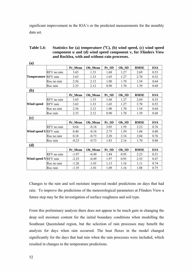
52
significant improvement in the IOA’s or the predicted measurements for the monthly
data set.
Table 5.4: Statistics for (a) temperature (oC), (b) wind speed, (c) wind speed component u and (d) wind speed component v, for Flinders View and Rocklea, with and without rain processes.
(a) Pr_Mean Ob_Mean Pr_SD Ob_SD RMSE IOA
RFV no rain 3.65 1.33 1.68 1.27 2.69 0.53 RFV rain 3.63 1.33 1.65 1.27 2.70 0.52 Roc no rain 2.56 2.12 1.00 1.70 1.54 0.64
Temperature
Roc rain 2.33 2.12 0.90 1.70 1.39 0.68 (b)
Pr_Mean Ob_Mean Pr_SD Ob_SD RMSE IOA RFV no rain 3.65 1.33 1.68 1.27 2.69 0.53 RFV rain 3.63 1.33 1.65 1.27 2.70 0.52 Roc no rain 2.56 2.12 1.00 1.70 1.54 0.64
Wind speed
Roc rain 2.33 2.12 0.90 1.70 1.39 0.68 (c)
Pr_Mean Ob_Mean Pr_SD Ob_SD RMSE IOA RFV no rain 0.64 -0.18 3.05 1.59 2.23 0.76 RFV rain 0.40 -0.18 2.75 1.59 1.88 0.80 Roc no rain 0.18 -0.73 2.20 2.16 2.04 0.76
Wind speed U
Roc rain -0.23 -0.73 1.83 2.16 1.70 0.80 (d)
Pr_Mean Ob_Mean Pr_SD Ob_SD RMSE IOA RFV no rain -1.97 -0.49 1.84 0.95 2.23 0.51 RFV rain -2.25 -0.49 1.97 0.95 2.52 0.47 Roc no rain -1.26 -1.01 1.13 1.16 1.11 0.74
Wind speed V
Roc rain -1.35 -1.01 1.09 1.16 1.08 0.75
Changes to the rain and soil moisture improved model predictions on days that had
rain. To improve the predictions of the meteorological parameters at Flinders View a
future step may be the investigation of surface roughness and soil type.
From this preliminary analysis there does not appear to be much gain in changing the
deep soil moisture content for the initial boundary conditions when modelling the
Southeast Queensland region, but the selection of rain processes may benefit the
analysis for days when rain occurred. The heat fluxes in the model changed
significantly for the days that had rain when the rain processes were included, which
resulted in changes to the temperature predictions.

53
The high wind speed observed on the 14th of June was observed at all sites, but it was
not predicted by the model at any of them. (While the wind speed was predicted at
Flinders View it was only due to the model continually overpredicting at this site.) On
closer investigation this was because this phenomenon was not included in the
synoptic information that is fed into TAPM as an input. Therefore, the model cannot
be expected to be able to pick this event if the information is not available to it.

54
Figure 5.15: Comparison of observed temperature with predicted temperature (with and without rain and change in soil moisture) for Rocklea
Figure 5.16: Comparison of observed wind speed with predicted wind speed (with and without rain and change in soil moisture) for Rocklea

55
Figure 5.17: Comparison of observed temperature with predicted temperature (with and without rain and change in soil moisture) for Flinders View
Figure 5.18: Comparison of observed wind speed with predicted wind speed (with and without rain and change in soil moisture) for Flinders View

56
5.2.2 Selection of roughness length
Closer inspection of the vegetation category in TAPM for the area surrounding
Flinders View, identified grassland as the default land use type. The canopy height
for this category is 0.6 m, resulting in a roughness length of approximately 0.06 m.
Visual inspection of the monitoring site showed that the roughness length was much
greater. Since the monitoring site is located within a residential area, with forest
within a few kilometers, the urban land use was selected (as the canopy height of 10
m gives an approximate surface roughness of 1.0 m) and the month of June was re-
modelled (with rain processes on).
The results (Figure 5.19-20) illustrated a significant improvement in the prediction of
wind speed throughout the month of June even though the wind speed remained
overestimated. The mean observed wind speed for June was 1.3 ms-1 compared with
2.3 ms-1 for urban landuse and 3.6 ms-1 for the original TAPM run. The temperature
predictions did not improve, in fact generally for the month of June the results were
worse with the predicted minimum temperatures significantly higher (2-4oC) than the
observations. This is due to Flinders View not being an urban site. The heat fluxes
such as sensible heat and evaporative heat were investigated to check whether
temperature was dependent on these values. If it was, one would expect little change
in the fluxes between model runs, however there was a significant difference in the
heat fluxes for the different land use categories. It can be concluded that temperature
is very dependent on the heat fluxes.
The selection of urban land use with TAPM selects an alternate group of algorithms in
the model that deal with reproducing the wind parameters over urban areas (with the
model assuming that the land surface has the properties of concrete). This would
explain why the temperatures are much warmer and a better option would have been
to select a vegetation category with parameters similar to the vegetation at Flinders
View as it is on the edge of the urban area, not within it.
The wind direction is not improved by changes in the roughness length.

57
Figure 5.19: Timeseries of temperature and wind speed at Flinders View
(a) temperature
(b) wind speed
NOTE: Observations denoted by blue line, original TAPM run (vegetation = grassland) denoted by pink line and new TAPM run (vegetation = urban) denoted by green dashes).

58
Figure 5.20: Timeseries of (a) evaporative heat flux and (b) sensible heat flux at Flinders View for vegetation of grassland and vegetation of urban
(a) evaporative heat flux
(b) sensible heat flux
NOTE: Original TAPM run (vegetation = grassland) denoted by pink line and new TAPM run (vegetation =
urban) denoted by green dashes).

59
5.2.3 Sensitivity to soil type
Weather forecasting work conducted by Makar et al (2005) indicted that changes to
the heat fluxes had a significant impact on wind speed and temperature at the surface.
Soil type is another variable in TAPM that the user can select that can have a
significant effect on evaporative heat flux and sensible heat flux. A brief comparison
between two different soil types (with all other defaults kept the same was
conducted). For Flinders View the default soil type was sandy clay loam. The grid
point next to this one within the model was designated as clay. Figure 5.21 shows the
differences in wind speed and temperature between the two sites as well as the heat
fluxes. There are significant differences in the wind speed particularly and the
temperature and consideration should be given to the soil type chosen.
Figure 5.21: Timeseries of (a) temperature, (b) wind speed, (c) evaporative heat flux and (d) sensible heat flux for sandy clay loam soil and clay soil
(a) temperature

60
(b) wind speed
(c) evaporative heat flux

61
(d) sensible heat flux
5.2.4 Sensitivity to data assimilation
TAPM v 2.0 includes data assimilation as an option to help force the surface winds to
be modelled correctly. The month of June was rerun with the inclusion of Amberley
wind speed and wind direction data for June 1999. The weighting of the input data
was given as 1.0 and the radius of influence was 10 km. As expected there were
improvements in wind speed predictions at Flinders View due to its close proximity to
Amberley.
Data assimilation was not included in this work for the sites used for model
comparison. Good model evaluation should include comparison of modelled
information with field data unrelated to the inputs within the model.
5.2.5 Sensitivity to grid resolution
An analysis of TAPM’s sensitivity to the grid resolution was conducted to determine
whether local features such as topography in each nested grid were influencing air
movements. This was important due to the complexity of the topography in Southeast
Queensland, particularly with the Range to the north and south. Figure 5.22 illustrates

62
the similarity between the 1 km, 3 km and 6 km grid resolutions for wind speed.
Table 5.5 shows there is not much difference in the annual mean temperatures and
wind speeds for modelled data.
Table 5.5: Predicted annual temperature and wind speed for various grid resolutions at Flinders View.
Temperature Wind Speed
Observed mean 19.1 1.45
Predicted mean 1 km 19.23 3.55
Predicted mean 3 km 19.18 3.71
Predicted mean 6 km 19.21 3.51
Figure 5.22: Predicted wind speed at Flinders View for the 1 km, 3 km and 6 km resolution grids.
5.3 Performance of model based on cluster types
To seek more detailed information on performance, the index of agreement was
calculated for each cluster type to determine whether particular day types were
modelled more accurately by the model than others.

63
Figure 5.23 illustrates a box and whiskers plot of the index of agreement for each
cluster type. The cluster types with high and low IOAs are listed in Table 3.4.
Figure 5.23: Box and whisker plot of IOA for each cluster type for wind speed each site.
Table 5.6: Best (IOA>0.8) and worst (IOA<0.5) cluster types based on IOA based on predictions of the model (wspd and wdir)
Sites Good agreement Poor agreement
Rocklea 24, 21 1, 3, 6, 14
Eagle Farm 24, 22, 23, 20, 21, 2 3, 4, 6
Flinders View 22, 23, 20 6, 29, 11, 8, 15
Deception Bay 23, 22, 24, 20 1, 29, 3
Moreton 5, 16 23, 18, 26
Assessment of the best and worst cluster types using the index of agreement,
suggested that the day types that were more typical of summer and spring days were
modelled more accurately than winter days. Clusters 24 and 22 were predominantly
summer days with hot moderate northeasterly winds in the afternoon, while clusters
14 and 15 are more typical of winter days with cool light to moderate winds in the
afternoon from the north to easterly sector.

64
Investigating model performance based on cluster type provides more detail than
looking at 1999 as a whole year. However, in appreciating which cluster types are
predicted better than others, better clarification can be sought through looking at
cluster types that are important for a particular application. Assuming, that dispersion
of pollution is the application of interest, assessing the accuracy of the model for
cluster types that are known to be pollution-conducive days may give substantially
more information than the general annual statistics. Based on information in Section
3.2, days with warm light north-northwesterly winds in the morning changing to hot
moderate north-northeasterly winds in the afternoon at Eagle Farm (BOM station),
can be conducive to high ozone events (Cluster 27) as can very warm light
southwesterly winds in the morning changing to moderate northeasterly winds in the
afternoon (Cluster 23). The winter days with cool light to moderate winds in the
afternoon from the north to easterly sector associated with high pressure systems
(Cluster 14 and 15) can also be conducive high pollution events, with elevated NOx
concentrations observed during the morning between 7 am and 9 am. Further analysis
of the diurnal profile for these days could elicit more information about the model’s
performance. In Appendix D the diurnal profiles for summer and winter cluster types
reviewed here are presented.
5.3.1 Diurnal profiles of wind speed and temperature
Previously in this work the diurnal profile for the mean wind speed was presented for
Deception Bay. The results showed that on average the predicted wind speed was
consistently 2 ms-1 higher than the observed wind speeds for each hour. The
differences between the predicted wind speed and observed wind speed for a summer
cluster type day and a winter cluster type day for Deception Bay are shown in Figure
5.24. The results illustrated very different profiles for wind speed. For the summer
day type the late afternoon breeze is underpredicted by the model (mean difference
approximately 2 ms-1), whereas for the winter day type for the same period the wind
speed was overpredicted by the model (mean difference 3 ms-1).
The mean difference between predicted and observed wind speeds during the day for
summer cluster day types is less than 0.5 m/s whereas for winter it is much higher.
This difference in wind speeds is due to the wind direction. For the summer cluster

65
days the wind direction during the day (7 am to 4pm), predicted by the model was
predominantly northwesterly, whereas for the winter days investigated the
predominant wind direction was southeasterly for the same time period. Analysis of
the overall wind speed for the year showed that the greatest difference in predicted
and observed wind speeds at Deception Bay resulted when winds were blowing from
the southeast, therefore it is not surprising that the diurnal profile for the winter days
demonstrates a different profile than for summer.
The diurnal profiles of the difference between predicted and observed temperatures at
Flinders View for the two synoptic cluster types is shown in Figure 5.25. The annual
predicted mean temperature shown previously showed very little difference to the
observed mean temperature. The mean difference in temperature at Flinders View for
the winter cluster type illustrates that the temperatures before midday are over
predicted compared with the afternoon, night temperatures. The frequency of winds
tends to be from the southeast in the afternoon (better prediction), where as the wind
direction tends to be predominantly south to southwesterly in the morning.
The profiles of wind speed at Flinders View illustrate that the sea breeze on the
summer days tends to be overpredicted by the model, whereas the winter wind speed
seems to be consistently overpredicted.
Each profile provides a little more detail about every site. For Rocklea the wind
speed profiles are very similar for the summer and winter cluster type. The afternoon
wind speeds are underpredicted for each season by the model. This appears to be
independent of wind direction (for this example) as the main wind direction in the
afternoon for winter is southeasterly and northeasterly for summer, yet the same
profiles are seen. Whereas TAPM overpredicts the afternoon wind speed for winter
day types and underpredicts for the summer day types at Eagle Farm.
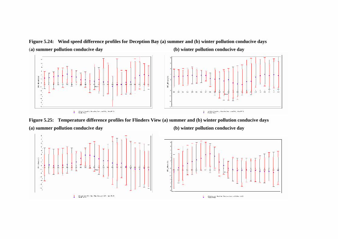
Figure 5.24: Wind speed difference profiles for Deception Bay (a) summer and (b) winter pollution conducive days (a) summer pollution conducive day (b) winter pollution conducive day
Figure 5.25: Temperature difference profiles for Flinders View (a) summer and (b) winter pollution conducive days
(a) summer pollution conducive day (b) winter pollution conducive day

67
5.3.2 Case day 30 January 1999
January 30, 1999 was selected for further investigation into model performance. It is
an example of a typical summer day that is conducive to high pollution episodes.
Based on monitoring information of ozone concentrations at each of the four
monitoring locations it was selected as a high pollution day for 1999. Hourly ozone
concentrations at all sites were above 6 pphm with the highest concentrations
recorded at Deception Bay (9.15 pphm) and Flinders View (6.75 pphm). There were
no records of bush fires or dust events that may have contributed to the higher
concentrations.
Time series figures of wind speed and wind direction for the 30th January provide
important information about the northeasterly change in the afternoon. For Deception
Bay and Eagle Farm the highest ozone concentrations were recorded at 11 am in the
morning of the 30th January.
Figure 5.26a illustrates the arrival of a moderate sea breeze by 10 am which remains
for most of the day as observed at Deception Bay. The sea breeze is predicted to occur
for a similar time period, with slightly stronger winds in the afternoon. This may lead
to the dispersion of the pollution to be greater than in reality for the afternoon.
Figure 5.26c and d illustrate the early prediction of the sea breeze by the model at
Rocklea (3 hours early) and Flinders View (2 hours early). Of particular interest is
that when the sea breeze arrives at Flinders View as predicted by the model the wind
speed increases dramatically from 1 ms-1 to 7 ms-1 which is not mirrored in the
observational data. This could have a significant impact on the subsequent prediction
of pollution concentrations at this site, particularly as the elevated levels of ozone
were observed to occur at 4 pm (same time as the model predicted 7 ms-1 winds).

Figure 5.26: Timeseries plots of wind direction and wind speed for (a) Deception Bay, (b) Eagle Farm, (c) Rocklea and (d) Flinders View, 30 January 1999, ozone pollution conducive day
(a) Deception Bay
(b) Eagle Farm

(c) Rocklea
(d) Flinders View

70
5.3.3 Case day 5 March 1999
The other example of a day identified as significant for ozone pollution was the 5th of
March (Cluster type 23). This day is characteristic of the typical sea breeze afternoons
that are experienced in summer in Southeast Queensland. The arrival and strength of
this sea breeze is extremely important in the dispersion of pollutants from the City to
the more southwestern districts. Days that fit into this category exhibit abrupt changes
in wind direction in the afternoon with an onshore wind blowing all the way to
Amberley. The 5th of March was selected for closer examination as the IOA suggested
that the model predicted the wind direction, wind speed and temperature satisfactorily.
It is interesting that for this day the model was able to predict the change in the wind
direction at all four sites, on the hour, with the easterly winds remaining for up to five
hours. Closer inspection of the pollution data for this day, suggested that perhaps
dispersion could be modelled well as the change in wind direction to the east and the
arrival of the sea breeze at each of the sites coincided with the maximum ozone
concentrations observed.
The maximum wind speed is over predicted by the model for most of the sites.

Figure 5.27: Timeseries plots of wind direction and wind speed for (a) Deception Bay, (b) Eagle Farm, (c) Rocklea and (d) Flinders View, 5 March 1999, ozone pollution conducive day
(a) Deception Bay
(b) Eagle Farm

(c) Rocklea
(d) Flinders View

73
5.3.4 Case day 21 June 1999
The 21st June was identified as a high NOx pollution day, typical of winter time
pollution. For winter time NOx pollution events, elevated concentrations of NOx are
observed generally between 7 am to 9 am when the wind speeds are light, and the air
more stagnant leading to an accumulation of pollution until the wind speed picks up
and disperses the pollution. This accumulation of pollution may on occasions be
emissions from the previous day.
The indices of agreement have shown that TAPM generally predicts these day types
less satisfactorily than summer day types. In particular the wind speed in the early
hours of the morning is overpredicted on this day by 50 to 200 % before 10 am at all
locations. The wind direction is predicted quite well in the early hours of the morning
at the coastal sites of Deception Bay and Eagle Farm while there is quite different
wind directions predicted at the more inland sites of Rocklea and Flinders View. It is
interesting to note that on these winter pollution type days the days are more stable.
The overprediction of the nighttime winds by the model may lead to very significant
differences to any pollution modelling conducted and the pollution observed.
Overprediction of these morning winds could lead to early dispersion of pollution and
the morning peak concentrations will not be predicted.
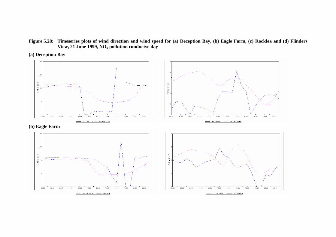
Figure 5.28: Timeseries plots of wind direction and wind speed for (a) Deception Bay, (b) Eagle Farm, (c) Rocklea and (d) Flinders View, 21 June 1999, NOx pollution conducive day
(a) Deception Bay
(b) Eagle Farm

(c) Rocklea
(d) Flinders View


77
6. Discussion
Due to the growing use of TAPM as a meteorological processor for areas where there
is no or poor observational data the model was run for one year using the defaults for
soil moisture and sea surface temperatures as well as without rain processes on.
The model was compared to observational data at five monitoring sites across
Southeast Queensland. Each site was unique due to its location A preliminary
analysis of the mean wind speed and temperature showed that the meteorology at the
urban sites were modelled well, while the difference in predicted and observed data at
the urban fringe sites was slightly greater, with the general trend being that the wind
speed is overpredicted by the model. The wind speed was overpredicted by 12 % to
143% depending on the location of the site, which was quite similar to the results
found by Hibberd et al (2003), where for various sites studied in Western Australia
the wind speed was overpredicted between 31% to 105%. Jackson et al (2003) also
found that overall wind speeds were overpredicted at a variety of sites across
Australia, irrespective of their relative location to the coast. This then suggests that
how the surface rougheness is treated in the model, may not adequately represent
reality. For Moreton Island, a complex site for any model to adequately predict, the
temperature was significantly overpredicted but this was due to the model treating the
site as a water location. The seasonal months of summer and spring tended to be
modelled to better accuracy than the autumn and winter months. Investigation of the
frequency distributions of the wind direction suggested that there may be a few
problems with the wind direction.
Closer examination of the observational data for the month of June, showed that for
1999, it was an extremely wet month. Wetter than the average in the last 25 years.
TAPM was rerun for June with the inclusion of rain. (Inspection of the temperature
timeseries suggested that the model was not adequately predicting the cloud cover,
hence not correctly determining the heat fluxes and subsequent temperature as the
predicted minimum temperatures were much warmer than observed across the sites.)
The model predictions (with the inclusion of rain processes) provided better
agreement between observational and modelled data at Rocklea for days on which it

78
actually rained. From this it can be recommended that if there is knowledge of high
rain that the inclusion of rain processes within the model may give some
improvement. Therefore for all model runs rain processes should be included.
However, the issue of inadequate cloud cover calculations (resulting in much warmer
predicted minimum temperatures) is still unresolved and further work is needed.
The model performance at the urban fringe site of Flinders View was not satisfactory
for the prediction of wind speed but this may be a consequence of the monitoring site
location rather than model performance. The high wind speeds predicted from the
model suggested that the monitoring site may not be adequately represented through
the selection of vegetation, similar to results discussed in Hibberd et al (2003). The
high wind speeds would suggest that there was not enough surface roughness to slow
the winds down. The vegetation was changed from grassland to urban (as the actual
monitoring location is in a residential area surrounded by forest) for a radius of 6 km
around the site. Re-running the model showed a significant improvement in the wind
speeds. The effect of soil type selection was also investigated. Changes to the soil
type affected the heat fluxes, but the full extent of the impact this has on the
modelling is yet to be evaluated. These studies confirmed that the user must carefully
prescribe the vegetation and soil type parameters within the model.
Data assimilation was used for a site 6 km from Flinders View. While this improved
the wind speed performance yet again, there was no improvement to the wind
direction or temperature profiles at Flinders View due to the distance away from the
site. Luhar et al (2004) found there was significant improvement in all surface
meteorological parameters (temperature, wind speed and wind speed components U
and V when data assimilation was included, however the sites investigated in that
study where much closer to the actual location of the observed data included for data
assimilation.
Using the index of agreement as a statistical measure allows for a quick evaluation of
model performance, however can be limiting in providing information where a model
may or may not perform well.

79
Cluster analysis was used to categorise days into smaller subgroups based on synoptic
characteristics. This allowed for more detailed interest as one could look at days of
interest for a particular application. It enabled the identification of the types of days
that the model predicted well and the ones the model didn't. Days that were typical of
summer conditions were modelled better than days typical of winter conditions.
Cluster types were then grouped further through determining pollution conducive
days, that is the cluster types that are typical for ozone pollution conducive days and
cluster types for winter pollution days.
Cluster 27, which was extremely similar to the day types previously investigated by
Coffey (1993), Physick (1993). These days in the morning had light north-
northwesterly winds which changed to very warm moderate north-northeastlery winds
in the afternoon at Eagle Farm. The model over predicted parameters at some sites
and underpredicted at others. Further investigation of the diurnal profiles determined
that for that particular day it is the onshore winds in the afternoon that are important
for polllution dispersion. The 30th January was investigated further Sea breeze was
predicted early in some cases and at twice the strength.
Another ozone conducive day type was evaluated, Cluster 23. These days typically
had light very light west-southwesterly winds in the morning before coming warm
moderate easterly winds in the afternoon at Eagle Farm. At Amberley Airport light
northwesterly morning winds were observed to change to hot easterly winds in the
afternoon. The daily wind direction and wind speed profiles for the 5th March were
evaluated. On this occasion the model predicted the sea breeze very well. Further
investigation is required to determine why this day the afternoon breeze was predicted
well, while there was a delay for the 30th January.
Winter pollution conducive days (elevated NOx concentrations) were investigated
(Cluster 14 and 15). These days were typically associated with cool, light to moderate
winds in the afternoon from the north to easterly sector combined with a high pressure
system. The results illustrated very different profiles for wind speed at each of the
sites compared with the summer profiles. In the early hours of the morning wind
speeds were generally overpredicted for most sites in winter.

80
Viewing the diurnal profiles of significant cluster types provided more information
about the performance of the model, than the mean profiles for wind speed and wind
direction. It showed that across sites, the differences in wind speed and temperature
can vary, and understanding why these variations occur is very important for correct
analysis of model outcomes.
Depending on the application for the modelling work being undertaken the additional
methods of evaluating the model performance such as the fractional bias will assist in
assessing the parameters that are significant for the particular application.

81
7. Conclusions
TAPM is a powerful prognostic meteorological modelling tool. Databases for terrain,
synoptic meteorology, land use and vegetation, and soil types are included with the
package on purchase eliminating the need for additional site-specific information to
be included in the model inputs. It appears very simple to use if the defaults and
databases are used. TAPM is being increasingly used to generate surface
meteorological statistics for dispersion modelling assessments, particularly (but not
exclusively) where there are not field data/observations.
The results showed that TAPM predicted the surface meteorology satisfactorily. The
use of synoptic clusters helps in data validation because it helps to understand what
wind speed and wind direction phenomenon is predicted or not predicted in the
model. This may provide useful feedback for ongoing model fine-tuning. It is
essential to include the appropriate land use, vegetation and soil type to maximise
model performance.
Overall TAPM adequately represented the air flows in the Southeast Queensland
airshed. The following were found:
• Annual average temperature and wind speed statistics were modelled well. At
most sites the annual average temperature was overpredicted by 1.3 oC and the
annual average wind speed by 0.5 m/s.
• The distribution of wind direction frequency remains a concern, however if the
regional wind flows (which were modelled satisfactorily) are the winds of
interest rather than the local winds then perhaps the prediction of local flows
around each station is not as important.
• TAPM satisfactorily predicts the sea breeze on synoptic day types
representative of sea breeze days. On some days in particular the arrival of the
sea breeze in the afternoon is predicted within an hour of what is observed at
the monitoring stations. On other days it may be a few hours late.
• The strength of the sea breeze is over predicted at the sites such as Deception
Bay and Flinders View. The wind speed was underpredicted at the urban sites.

82
• The wind direction on winter mornings (that may see recirculation) does not
appear to be modelled well.
• The wind speed on winter pollution conducive days was modelled
satisfactorily. The accuracy of the wind speed predictions tended to be reliant
on the direction of the wind flows. Windspeeds from the northeast and
northwest were predicted better than winds from the southeast.
• The differences in modelled and observed temperatures also seemed to be
dependent on wind direction.
The method of evaluation used in this work provided useful information about the
model performance and reliability on observational data.
• The standard statistical methods of mean, standard deviation and index of
agreement allowed for assessment of annual averages of wind speed and
temperature.
• Subsets of the annual data into seasonal and diurnal variation provided insight
into when TAPM predicted the observations well and when it didn't.
• Synoptic clustering and determination of significant clusters based on summer
ozone and winter pollution conducive days allowed easy evalution of the
performance of the model for days which were deemed important for
dispersion. This allowed another level of detail that the previous statistical
methods didn't. It provided a good first step, especially if diurnal behaviour of
residuals is investigated.
• Selection of observational data sets is important. In identifying the surface
boundary layer conditions of each of the monitoring stations it was easy to
ascertain which sites the model should not be expected to predict accurately.
For Flinders View and Deception Bay the locations of trees within a few metres
of the sites, caused concern that the monitoring instruments may be sheltered
and therefore deviations of wind speed, wind direction and temperature
paramters may result. The complexity of both of these sites due to surrounding
terrain and coastline could cause local effects that would not be expected to be
predicted by the model.
Varying the inputs into the model showed the following when the model is used for
the Southeast Queensland airshed:

83
• The selection of vegetation type/land use is very important. Changes in the heat
fluxes, tempertures and wind speed predictions occurred. Care should be taken
when determining whether an area is to be classified as urban as it appears that
the workings within the model may cause overestimation of surface
temperature to be greater than what is observed.
• The selection of soil type affected the surface heat fluxes significantly and
subsequently affected ground-level temperature and wind speed predictions
within the model.
• The effect of the selection of rain processes varied for each site, however, this
variation at each site was probably more to do with the way the site was
represented rather than the selection of the rain processes. The inclusion of rain
processes is not expected to hamper the performance of TAPM, therefore
should be selected as on.
• Data assimilation did improve wind speed at Flinders View when it was
included for a site nearby. Should reliable wind speed and wind direction data
exist within 10 km of the site, this can be included within the model to assist in
predicting the correct wind flows. At a distance further than this it is unlikely
that data assimilation will improve performance because it will beyond the
radius of influence.
• The various grid resolutions used for this modelling showed little variation
between annual average predictions of wind speed and wind direction.
However, this may not be the case for all model set ups. Verifying that terrain
information is adequately represented is important as the averaging of terrain of
1km2 or greater may cause a loss of features such as valleys and mountains.
Going to much finer resolution, may have showed quite different results.
• The selection of deep soil moisture content alone did not improve the overall
performance of TAPM significantly.

84

85
8. References
ASTM (2000) Standard guide for statistical evaluation of atmospheric dispersion
model performance, Designation: D6589-00. American Society for Testing and
Materials, West Conohocken, PA.
Azzi M., Hyde R., and Duc H. (2002) Comparison of predicted and observed
temperature and wind profiles on a high ozone event in Sydney. Proceedings of the
16th International Clean Air and Environment Conference. Christchurch, New
Zealand, 2002, Clean Air Society of Australia & New Zealand.
Coffey Partners International Pty. Ltd., (1993) Brisbane Wind-field Study: Final
report to Department of Environment and Heritage. Report E184/1 May 1993.
Department of Environment (Qld), 1997 Air Quality in the southeast Queensland air
shed – State of Knowledge Report.
Elbir T. (2003) Comparison of model predictions with the data of an urban air quality
monitoring network in Izmir, Turkey. Atmospheric Environment 37, 2149-2157.
Graham L. and Bridgman H. (2002) Applying The Air Pollution Model (TAPM), in
the Lake Macquarie airshed. Proceedings of the 16th International Clean Air and
Environment Conference. Christchurch, New Zealand, 2002, Clean Air Society of
Australia & New Zealand. pp 270-273
Hibberd M, Physick, B and Park G. (2003) Verification of several aspects of TAPM
against multi-year monitoring data at Collie. Proceedings of the 17th International
Clean Air Conference. Newcastle, New South Wales, 2003, Clean Air Society of
Australia.
86
Hurley P. (2000) Verification of TAPM meteorological predictions in the Melbourne
region for a winter and summer month. Aust. Met. Mag 49, 97-107.
Hurley P. (2001) The Air Pollution Model (TAPM) Version 2. Part 1: Technical
Description. CSIRO Atmospheric Research Technical Paper No.55
Ischtwan and Cope (1996) Modelling of photochemical smog in the South East
Queensland airshed. Environment Protection Authority, Victoria, 1996.
Ischtwan (2002) Prognostic modelling of a summer period of photochemical smog in
southeast Queensland. Proceedings of the 16th International Clean Air and
Environment Conference. Christchurch, New Zealand, 2002, Clean Air Society of
Australia & New Zealand.pp360 - 365
Internet: http://www.dar.csiro.au/ladm/
Internet: http://www.dar.csiro.au/tapm/
Jackson L, Leishman N, Killip C and Best P (2003) Windfield prediction and
verification for a variety of sites across Australia. Proceedings of the 17th
International Clean Air Conference. Newcastle, New South Wales, 2003, Clean Air
Society of Australia.
Johnson GM, (1992) An evaluation of selected photochemical smog events for the
Brisbane region. Report to Brisbane City Council.
Killip C.A., Brooke A.S., Jackson L.D., Best P.R., Verrall K. and Wainwright D.
(2002) Advanced modelling tools for air quality management – Gladstone 10 years
on. Proceedings of the 16th International Clean Air and Environment Conference.
Christchurch, New Zealand, 2002, Clean Air Society of Australia & New Zealand.
422-428

87
Lorimer G. (1986) The AUSPLUME Gaussian dispersion model. Environment
Protection Authority of Victoria, publications no.264
Luhar A.K. and Hurley P.J. (2002) Evaluation of TAPM using the Indianapolis
(urban) and Kwinana (coastal) field data sets. Proceedings of the 16th International
Clean Air and Environment Conference. Christchurch, New Zealand, 2002, Clean Air
Society of Australia & New Zealand.
Luhar A.K. and Hurley P.J (2004) Application of a prognostic model TAPM to sea-
breeze floes, surface concentrations, and fumigating plumes. Environmental
Modelling & Software. 19, 591-601
Makar P.A., Gravel S., Chirkov V., Belair S., Strawbridge K., and Froude F. (2005)
The impact of anthropogenic heat and surface roughness on an operational weather
forecast. Geophysical Research Abstracts, 7. 01768,
Pielke, R.A. (1984) Mesocscale Meteorological Modelling Academic Press, Orlando.
Physick B., Blockley A., Farrar D., Rayner K, and Mountford P. (2002a) Application
of three air quality models to the Pilbara region. Proceedings of the 16th International
Clean Air and Environment Conference. Christchurch, New Zealand, 2002, Clean Air
Society of Australia & New Zealand.629-634.
Physick B.L., Hurley P.J, Blockley A., Rayner K.N. and Mountford P. (2002b)
Verification of the air quality models TAPM and DISPMOD in coastal regions.
Presented at 4th International Conference on Environmental Problems in Coastal
Regions. 16-18 September 2002. Rhodes, Greece.
Rao S.T., Zurbenco I., Neagu R., Porter P., Ku J.Y., Henry R. (1999) Space and time
scales in ambient ozone data. Bulletin of American Meteo. Soc., 78, 2153-2166.
Schlünzen K.H., Baechlin W., Brünger H., Eichhorn J., Grawe D., Schenk R., and
Christof Winkler (2004) 9th Int. Conf. on Harmonisation within Atmospheric
Dispersion Modelling for Regulatory Purposes, 147-150

88
Simpson RW and Auliciems A, (1989) Air pollution in Brisbane. Institute of Applied
Environmental Research, Griffith University, Nathan, Q4111, 109 pp.
Skjøth CA., Brandt J. and Christensen JH (2005) Validation methods in
meteorological and air pollution modelling. Paul Scherrer Institute www.psi.ch
Stone RC (1989) Weather types at Brisbane, Queensland: an example of the use of
principal components and cluster analysis. International Journal of Climatology, 9:3-
32.
Tustison, Foufoula-Georgiou E, and Harris D. (2003) Scale-recursive estimation for
multisensor Quantitative Precipitation Forecast verification: A preliminary
assessment. J Geophys Res. 107, D8, 2-1 – 2-14
Wilmott C.J. (1981) On the Validation of Models. Phys. Geography 2 184-94.

89
Appendix A - Meteorological component of TAPM
The mean horizontal wind components u and v are derived from the momentum equations (Hurley, 2001).
)()(''
ssv uuNfvxxz
uwuFdtdu
−−+⎟⎠⎞
⎜⎝⎛
∂∂
∂∂
+∂∂
−∂∂
∂∂
+=σ
σππθσ
σ
)()(''
ssv vvNfuyyz
vwvFdtdv
−−+⎟⎟⎠
⎞⎜⎜⎝
⎛∂∂
∂∂
+∂∂
−∂∂
∂∂
+=σ
σππθσ
σ
⎟⎟⎠
⎞⎜⎜⎝
⎛∂∂
∂∂
+⎟⎠⎞
⎜⎝⎛∂∂
∂∂
+⎟⎟⎠
⎞⎜⎜⎝
⎛∂∂
+∂∂
−=∂∂
yv
xu
yv
xu σ
σσ
σσσ&
where:
x,y, σ are the components of the coordinate system (m) θv is the potential virtual temperature, π is 3.14159265, Ns is the large scale nudging coefficient (1/(24x3600)) us, vs and θs are the large scale synoptic winds and potential virtual temperature,
⎟⎟⎠
⎞⎜⎜⎝
⎛−−
=sT
sT zz
zzzσ , where z is the Cartesian vertical coordinate (m), zT is the
height of the model top (m) and zs is the terrain height (m). Scalar equations are solved for potential virtual temperature
)()(''
vsvsv
vv NS
zw
Fdt
dv
θθσσθ
θθ
θ −−+∂∂
∂∂
+=
1−
⎟⎠⎞
⎜⎝⎛∂∂
−=∂∂
zg
v
H σθσ
π
where g is the gravitational constant (8.91ms-2)
vv qpradiation
v Sct
TT
S λθθ −⎟
⎠⎞
⎜⎝⎛∂∂
=
where T is temperature (K) λ is the latent heat of vaporisation of water (2.5x10⁶ Jkg-1) cp is the specific heat at constant pressure (1006 Jkg-1K-1)

90

91
Appendix B – Statistical Formulae
Statistics (based on Willmott, 1981 and Pielke, 1984) were calculated as follows:
Observed mean: ∑=
=N
iimean O
NO
1
1
Predicted mean: ∑=
=N
iimean P
NP
1
1
Observed Standard Deviation: ∑=
−−
=N
imeanistd OO
NO
1
2)(1
1
Predicted Standard Deviation: ∑=
−−
=N
imeanistd PP
NP
1
2)(1
1
Pearson Correlation Coefficient
⎥⎥⎦
⎤
⎢⎢⎣
⎡⎟⎠
⎞⎜⎝
⎛−⎟⎠
⎞⎜⎝
⎛
⎥⎥⎦
⎤
⎢⎢⎣
⎡⎟⎠
⎞⎜⎝
⎛−⎟⎠
⎞⎜⎝
⎛
⎟⎠
⎞⎜⎝
⎛⎟⎠
⎞⎜⎝
⎛−⎟⎠
⎞⎜⎝
⎛
=
∑∑∑∑
∑∑∑===
22
22
111
N
Ii
N
ii
N
Ii
N
ii
N
ii
N
ii
N
iii
PPNOON
POPONr
Root Mean Square Error: ( )∑=
−=N
iii OP
NRMSE
1
21
Unsystematic Root Mean Square Error: ( )∑=
−=N
iii PP
NURMSE
1
2ˆ1_
Systematic Root Mean Square Error: ( )∑=
−=N
iii OP
NSRMSE
1
2ˆ1_
Index of Agreement: ( )
( )∑
∑
=
=
−+−
−−= N
imeanimeani
N
iii
OOOP
OPIOA
1
2
1
2
1

92
P̂
Measures of Skill: stdP
URMSEESKILL __ =
std
std
OP
VSKILL =_
SKILL_R = stdP
SRMSEURMSE __ +
Where: N is the number of observations/predictions O is the Observed data P is the Predicted data
is the linear regression fitted formula with intercept a and slope b

93
Appendix C - Cluster definitions for cluster types
Cluster 1 EAG: Cold light southwesterly winds in the morning changing to warm light northerly winds by the afternoon followed by very light west-northwesterly winds overnight. AMB: Cold light west-northwesterly winds in the morning changing to warm light northwesterly winds in the afternoon.
Cluster 2 EAG: Warm light to moderate east-southeasterly winds in the afternoon changing to moderate northeasterly winds in the afternoon. AMB: Warm light easterly winds in the morning changing to moderate east-northeasterly winds in the afternoon High pressure system
Cluster 3 EAG: Warm light southwesterly winds in the morning changing to light northeasterly winds in the afternoon. Winds remaining from the northeasterly direction in the evening. AMB: Warm light westerly winds in the morning becoming slightly warmer in the afternoon.
Cluster 4 EAG: Very light cool winds in the morning, with north-northwesterly winds in the afternoon. Still very light conditions. AMB: Cool very light west-northwesterly winds in the morning, remaining light throughout the day
Cluster 5 EAG: Cool light to moderate westerly winds in the morning with winds strengthening in the afternoon. AMB: Cool moderate west-northwesterly winds strengthening to warm strong westerly winds.
Cluster 6 EAG: Warm light south-southeasterly winds. East-southeasterly winds in the afternoon. AMB: light south-southeasterly winds in the morning changing slightly to easterly in the afternoon. Warm day. Some rain
Cluster 7 EAG: Cold moderate west-southwesterly winds in the morning warming slightly during the day before becoming cooler light overnight winds. AMB: Cool light west-northwesterly winds in the morning changing to moderate westerly winds in the afternoon. High-pressure system, no rain.
Cluster 8 EAG: Warm moderate southerly winds becoming warmer throughout the day AMB: Warm moderate southerly winds becoming warmer throughout the day Low pressure system
Cluster 9 EAG: Cold moderate easterly winds, with a cool change in the afternoon.

94
AMB: Cool light southeasterly winds remaining light changing to easterly in the afternoon. Low pressure system, Very wet
Cluster 10 EAG: Warm moderate easterly winds in the morning, remaining the same throughout the day. AMB: Moderate easterly winds warming during the day but easing slightly Low-pressure system, Wet.
Cluster 11 EAG: Warm moderate to strong southerly winds becoming stronger southeasterly winds in the afternoon. AMB: Moderate warm south-southwesterly winds in the morning strengthening during the day.
Cluster 12 EAG: Warm light to moderate southerly winds changing to easterly in the afternoon. AMB: Very light southerly winds changing to light to moderate easterlies in the afternoon.
Cluster 13 EAG: Warm light to moderate south-southwesterly winds remaining the same throughout the day. AMB: Light to moderate southerly winds remaining the same throughout the day.
Cluster 14 EAG: Cool moderate southwesterly winds changing to warm moderate east-northeasterly winds in the afternoon before cooling and becoming still overnight. AMB: Cool very light west-southwesterly winds changing to warm light northeasterly winds.
Cluster 15 EAG: Cold moderate southwesterly winds changing to easterly winds in the afternoon becoming cold light southerly winds in the evening. AMB: Cool light west-southwesterly winds changing to warm very light easterly winds in the afternoon.
Cluster 16 EAG: Warm strong westerly winds strengthening throughout the day. Temperatures reaching the high 20s. AMB: Warm moderate westerly winds in the morning strengthening to very strong westerlies Low pressure system
Cluster 17 EAG: Warm very strong southeasterlies becoming stronger during the day. Temperatures reaching the high 20s. AMB: Warm moderate east-southeasterly winds in the morning. Winds in the afternoon are very strong easterly winds. High pressure system
Cluster 18 EAG: Warm moderate northerly winds becoming warmer in the afternoon with strong north-northeasterly winds before cooling slightly in the evening as winds are moderate northerly.

95
AMB: Warm light north-northwesterly winds in the morning changing to hot moderate easterly winds in the afternoon.
Cluster 19 EAG: Warm moderate southerly winds in the morning changing slightly to southeasterly in the afternoon. AMB: light to moderate south-southeasterly winds in the morning changing to east-southeasterly in the afternoon. High pressure system
Cluster 20 EAG: Warm light to moderate northerly winds, changing to very strong north-northeasterlies throughout the day. AMB: Temperatures in the low 20s. Light northerly winds becoming hotter in the day as the winds become northeasterly.
Cluster 21 EAG: Warm moderate south-southeasterlies in the morning changing to easterlies in the afternoon. AMB: Temperatures in the mid 20s. Light southeasterly winds becoming moderate easterly winds in the afternoon.
Cluster 22 EAG: Very light warm easterly winds in the morning becoming warmer during the day with moderate east-northeasterly winds in the afternoon. Still warm in the evening with winds light and from the northerly direction. Temperatures reaching the high 20s. AMB: Warm light northeasterly winds becoming hot moderate east-northeasterly winds in the afternoon.
Cluster 23 EAG: Warm very light west-southwesterly winds in the morning becoming warmer moderate easterly winds in the afternoon before easing in the evening with north-northeasterly winds. Temperatures reaching the high 20s. AMB: Warm light northwesterly winds becoming hot easterly winds in the afternoon.
Cluster 24 EAG: Temperatures in the mid 20s, moderate easterly winds in the morning becoming warmer during the day. AMB: Warm light easterly winds with temperatures reaching high 20s as the moderate east-northeasterly winds arrive in the afternoon.
Cluster 25 EAG: Very strong easterlies throughout the entire day. AMB: warm moderate easterly winds in the morning becoming stronger during the day. Rain
Cluster 26 EAG: Cold strong west-southwesterly winds AMB: Temperatures in the low teens, with strong westerly winds. These winds strengthen throughout the day.
Cluster 27 EAG: Warm light north-northwesterly wind changing to very warm moderate north-northeasterly winds in the afternoon. Lighter winds in the evening. Temperatures reaching the high 20s. AMB: Very warm light northwesterly winds, changing to hot moderate west-

96
northwesterly winds. Cluster 28 EAG: Temperatures in the low twenties. Still morning with light to moderate
easterly wins in the afternoon. AMB: Very light northerly wind in the morning changing to easterly in the afternoons. Moderate rain
Cluster 29 EAG: Cold moderate south-southwesterly winds in the morning, warmer moderate southerly winds in the afternoon. AMB: Cold moderate southerly winds warming slightly during the day. Light Rain
Cluster 30 EAG: Temperatures in the mid teens before reaching twenties in the afternoon. Light to moderate south-southwesterly winds changing to easterly in the afternoon. AMB: very light southerly winds, becoming stronger slightly and easterly in the afternoon.

97
Appendix D Summer and winter/autumn pollution conducive days
Difference between predicted and observed data for autumn day type (Cluster 14); wind speed and wind direction for Deception Bay (a) wind speed
(b) wind direction

98
Difference between predicted and observed data for autumn day type (Cluster 14); temperature, wind speed and wind direction for Eagle Farm (a) temperature
(b) wind speed
(c) wind direction

99
Difference between predicted and observed data for autumn day type (Cluster 14); temperature, wind speed and wind direction for Rocklea (a) temperature
(b) wind speed
(c) wind direction

100
Difference between predicted and observed data for autumn day type (Cluster 14); temperature, wind speed and wind direction for Flinders View (a) temperature
(b) wind speed
(c) wind direction

101
Difference between predicted and observed data for autumn day type (Cluster 14); temperature, wind speed and wind direction for Moreton Island (a) temperature
(b) wind speed
(c) wind direction

102
Difference between predicted and observed data winter day type (Cluster 15); wind speed and wind direction for Deception Bay (a) wind speed
(b) wind direction

103
Difference between predicted and observed data for winter day type (Cluster 15); temperature, wind speed and wind direction for Eagle Farm (a) temperature
(b) wind speed
(c) wind direction

104
Difference between predicted and observed data for winter day type (Cluster 15); temperature, wind speed and wind direction for Rocklea (a) temperature
(b) wind speed
(c) wind direction

105
Difference between predicted and observed data for winter day type (Cluster 15); temperature, wind speed and wind direction for Flinders View (a) temperature
(b) wind speed
(c) wind direction

106
Difference between predicted and observed data for winter day type (Cluster 15); temperature, wind speed and wind direction for Moreton Island (a) temperature
(b) wind speed
(c) wind direction

107
Difference between predicted and observed data for summer day type (Cluster 23); wind speed and wind direction for Deception Bay (a) wind speed
(b) wind direction

108
Difference between predicted and observed data summer day type (Cluster 23); temperature, wind speed and wind direction for Eagle Farm (a) temperature
(b) wind speed
(c) wind direction

109
Difference between predicted and observed data summer day type (Cluster 23); temperature, wind speed and wind direction for Rocklea (a) temperature
(b) wind speed
(c) wind direction

110
Difference between predicted and observed data summer day type (Cluster 23); temperature, wind speed and wind direction for Flinders View (a) temperature
(b) wind speed
(c) wind direction

111
Difference between predicted and observed summer day type (Cluster 23); temperature, wind speed and wind direction for Moreton Island (a) temperature
(b) wind speed
(c) wind direction

112
Difference between predicted and observed data for summer day type (Cluster 27); wind speed and wind direction for Deception Bay (a) wind speed
(b) wind direction

113
Difference between predicted and observed data for summer day type (Cluster 27); temperature, wind speed and wind direction for Eagle Farm (a) temperature
(b) wind speed
(c) wind direction

114
Difference between predicted and observed data for summer day type (Cluster 27); temperature, wind speed and wind direction for Rocklea (a) temperature
(b) wind speed
(c) wind direction

115
Difference between predicted and observed for summer day type (Cluster 27); temperature, wind speed and wind direction for Flinders View (a) temperature
(b) wind speed
(c) wind direction

116
Difference between predicted and observed data for summer day type (Cluster 27); temperature, wind speed and wind direction for Moreton Island (a) temperature
(b) wind speed
(c) wind direction


