
Mobile Robotics and Olfaction Lab, AASS, Örebro University
# 1
Achim J. Lilienthal
Room T1227, Mo, 11-12 o'clock (please drop me an email in advance)

# 3 DIP'14 © A. J. Lilienthal (Dec 16, 2014)
Now the Exam!?!
0

# 4 DIP'14 © A. J. Lilienthal (Dec 16, 2014)
Allowed Aids?
Exam?

# 5 DIP'14 © A. J. Lilienthal (Dec 16, 2014)
First Rule
Exam?

# 6 DIP'14 © A. J. Lilienthal (Dec 16, 2014)
Grading – ECTS o labs x 3
» all need to be passed » extra points for the exam possible (1/10 of the exam per lab)
o exam » counts 100% » > 50% of the points to pass » another example
• exam has 100 points, you have 63 + 15 = 77 points
Examination
<50 50 – 59 60 – 69 70 – 79 80 – 89 90 – 100 – E D C B A
<50 50 – 74 75 – 100 U G VG

# 9 DIP'14 © A. J. Lilienthal (Dec 16, 2014)
Relevant Topics?
Examination
# 10 DIP'14 © A. J. Lilienthal (Dec 16, 2014)
Part 1 - Introduction
1
# 11 DIP'14 © A. J. Lilienthal (Dec 16, 2014)
1.
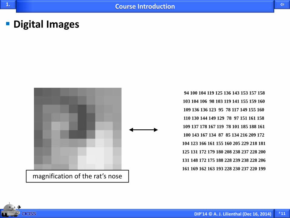
Digital Images
Course Introduction
94 100 104 119 125 136 143 153 157 158
103 104 106 98 103 119 141 155 159 160
109 136 136 123 95 78 117 149 155 160
110 130 144 149 129 78 97 151 161 158
109 137 178 167 119 78 101 185 188 161
100 143 167 134 87 85 134 216 209 172
104 123 166 161 155 160 205 229 218 181
125 131 172 179 180 208 238 237 228 200
131 148 172 175 188 228 239 238 228 206
161 169 162 163 193 228 230 237 220 199
magnification of the rat’s nose

# 12 DIP'14 © A. J. Lilienthal (Dec 16, 2014)
1.
Digital Images
Human Visual Perception o the human eye
Course Introduction

# 13 DIP'14 © A. J. Lilienthal (Dec 16, 2014)
1.
Digital Images
Human Visual Perception, E-M Spectrum
Course Introduction
νλ c=
νhE =

# 14 DIP'14 © A. J. Lilienthal (Dec 16, 2014)
1.
Digital Images
Human Visual Perception, E-M Spectrum
Image Formation – Pinhole Camera Model
Course Introduction
from Per-Erik Forssén "Visual Object Recognition"

# 15 DIP'14 © A. J. Lilienthal (Dec 16, 2014)
1.
Example Task
Exam?
Answer the following statements with either True or False. Note that you do not have to answer all the questions. Correct answers will be counted as +1 point and wrong answers as -1 point. Thus you should only answer those questions you are certain about. The total for this task cannot be, however, below 0. If the question ends with the sentence "explain your answer", you can get additional points by providing a more detailed answer to the corresponding question. No minus points will be assigned if the detailed answer is wrong.
a) The relation between subjective brightness and light intensity is approximately a log function. (1p) b) The visible spectrum can be specified in units of energy or in
wavelengths. Explain your answer. (3p)

# 17 DIP'14 © A. J. Lilienthal (Dec 16, 2014)
1.
Digital Images
Human Visual Perception, E-M Spectrum
Image Formation – Pinhole Camera Model
Image Formation – Illumination / Reflectivity o f(x,y) = i(x,y) r(x,y)
Course Introduction
# 18 DIP'14 © A. J. Lilienthal (Dec 16, 2014)
1.
Digital Images
Human Visual Perception, E-M Spectrum
Image Formation – Pinhole Camera Model
Image Formation – Illumination / Reflectivity
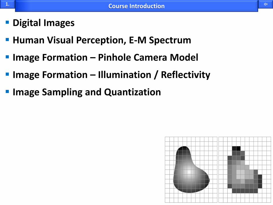
Image Sampling and Quantization
Course Introduction
# 19 DIP'14 © A. J. Lilienthal (Dec 16, 2014)
1.
Digital Images
Human Visual Perception, E-M Spectrum
Image Formation – Pinhole Camera Model
Image Formation – Illumination / Reflectivity
Image Sampling and Quantization
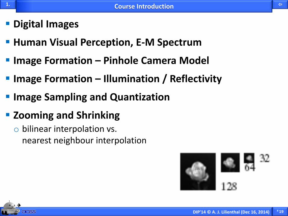
Zooming and Shrinking o bilinear interpolation vs.
nearest neighbour interpolation
Course Introduction
# 20 DIP'14 © A. J. Lilienthal (Dec 16, 2014)
1.
Digital Images
Human Visual Perception, E-M Spectrum
Image Formation – Pinhole Camera Model
Image Formation – Illumination / Reflectivity
Image Sampling and Quantization
Zooming and Shrinking and Rotation o bilinear interpolation vs.
nearest neighbour interpolation
Course Introduction

# 21 DIP'14 © A. J. Lilienthal (Dec 16, 2014)
Part 2 – Image Enhancement in the Spatial Domain
2

# 22 DIP'14 © A. J. Lilienthal (Dec 16, 2014)
2.
Image Enhancement
Spatial Domain Image Enhancement
more suitable for visual interpretation

# 23 DIP'14 © A. J. Lilienthal (Dec 16, 2014)
2.
Image Enhancement
Grey Level Transformations o 1x1 neighbourhood (point processing)
Spatial Domain Image Enhancement
)(rTs =)(rTs =

# 24 DIP'14 © A. J. Lilienthal (Dec 16, 2014)
2.
Matlab Questions?
Exam?
Which of the three images on the right is image fp (see Matlab code below) if the image on the left is f?
f = imread('bubbles.tif'); fp = imadjust(f, [0.1 0.9], [1.0 0.0], 0.5); imshow(fp);
f fp? (a) fp? (b) fp? (c)
⇒

# 26 DIP'14 © A. J. Lilienthal (Dec 16, 2014)
2.
Image Enhancement
Grey Level Transformations
Histogram Processing o what is a histogram o histogram equalization
Spatial Domain Image Enhancement

# 27 DIP'14 © A. J. Lilienthal (Dec 16, 2014)
2.
Image Enhancement
Grey Level Transformations
Histogram Processing o what is a histogram o histogram equalization o adaptive / localized
histogram equalization
Spatial Domain Image Enhancement

# 31 DIP'14 © A. J. Lilienthal (Dec 16, 2014)
2.
Linear Spatial Filtering o neighbourhood relations
» 4-neighborhood, 8-neighborhood
Spatial Filtering

# 32 DIP'14 © A. J. Lilienthal (Dec 16, 2014)
2.
Linear Spatial Filtering o neighbourhood relations o smoothing filters
» mean filter (box filter), Gaussian filter
Spatial Filtering
# 33 DIP'14 © A. J. Lilienthal (Dec 16, 2014)
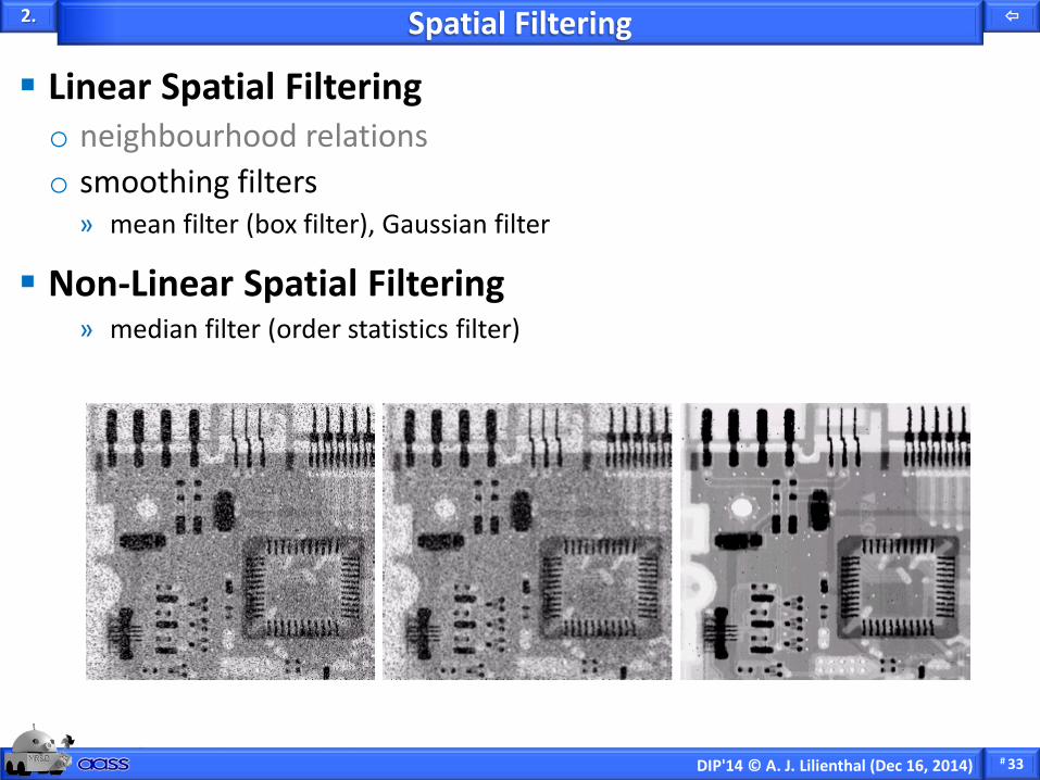
2.
Linear Spatial Filtering o neighbourhood relations o smoothing filters
» mean filter (box filter), Gaussian filter
Non-Linear Spatial Filtering » median filter (order statistics filter)
Spatial Filtering

# 34 DIP'14 © A. J. Lilienthal (Dec 16, 2014)
2.
Linear Spatial Filtering o neighbourhood relations o smoothing filters o sharpening filters (Sobel)
Spatial Filtering
1 0 -1
2 0 -2
1 0 -1
1 -2 -1
0 0 0
1 2 1

# 35 DIP'14 © A. J. Lilienthal (Dec 16, 2014)
2.
Linear Spatial Filtering o neighbourhood relations o smoothing filters o sharpening filters (Sobel, Laplacian)
Spatial Filtering
0 -1 0
-1 5 -1
0 -1 0
# 36 DIP'14 © A. J. Lilienthal (Dec 16, 2014)
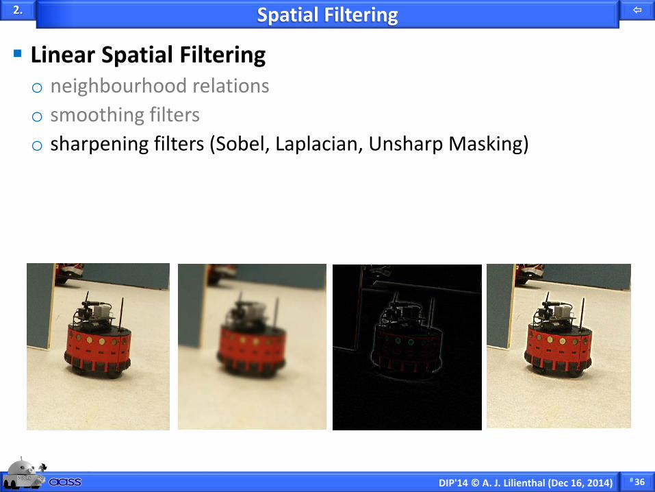
2.
Linear Spatial Filtering o neighbourhood relations o smoothing filters o sharpening filters (Sobel, Laplacian, Unsharp Masking)
Spatial Filtering

# 38 DIP'14 © A. J. Lilienthal (Dec 16, 2014)
Part 3 – Bilateral Filtering
3

# 39 DIP'14 © A. J. Lilienthal (Dec 16, 2014)
3.
Definition of the Bilateral Filter
Bilateral Filtering
space weight
not new
range weight
I
new
normalization factor
new
( ) ( )∑∈
−−=S
IIIGGW
IBFq
qqpp
p qp ||||||1][rs σσ
# 40 DIP'14 © A. J. Lilienthal (Dec 16, 2014)
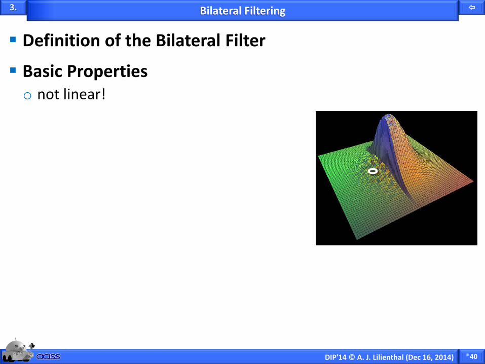
3.
Definition of the Bilateral Filter
Basic Properties o not linear!
Bilateral Filtering
# 41 DIP'14 © A. J. Lilienthal (Dec 16, 2014)
3.
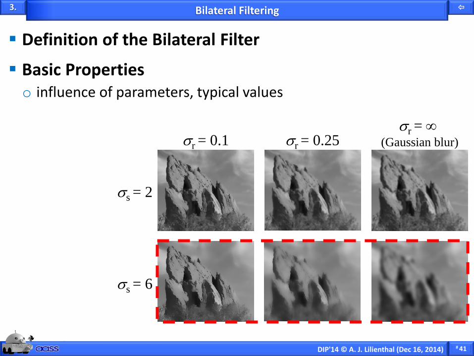
Definition of the Bilateral Filter
Basic Properties o influence of parameters, typical values
Bilateral Filtering
σs = 2
σs = 6
σr = 0.1 σr = 0.25 σr = ∞
(Gaussian blur)
# 42 DIP'14 © A. J. Lilienthal (Dec 16, 2014)
3.
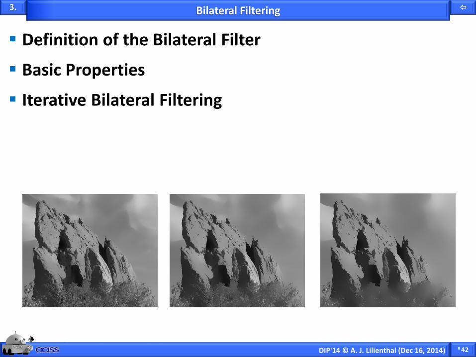
Definition of the Bilateral Filter
Basic Properties
Iterative Bilateral Filtering
Bilateral Filtering

# 43 DIP'14 © A. J. Lilienthal (Dec 16, 2014)
3.
Definition of the Bilateral Filter
Basic Properties
Iterative Bilateral Filtering
Bilateral Filtering Color Images
Bilateral Filtering
( ) ( )∑∈
−−=S
GGW
IBFq
qqpp
p CCCqp ||||||||1][rs σσ
3D vector (RGB, Lab, …)

# 44 DIP'14 © A. J. Lilienthal (Dec 16, 2014)
3.
Definition of the Bilateral Filter
Basic Properties
Iterative Bilateral Filtering
Bilateral Filtering Color Images
Many Applications o general idea useful in many different contexts
Bilateral Filtering

# 46 DIP'14 © A. J. Lilienthal (Dec 16, 2014)
Part 4 – Fourier Transform and Filtering in the Frequency Domain
4

# 47 DIP'14 © A. J. Lilienthal (Dec 16, 2014)
4.
Discrete Fourier Transform
Filtering in the Frequency Domain
→
sampled (0, 1, …, 128-1) spectrum = |F(u)| →
# 48 DIP'14 © A. J. Lilienthal (Dec 16, 2014)
4.
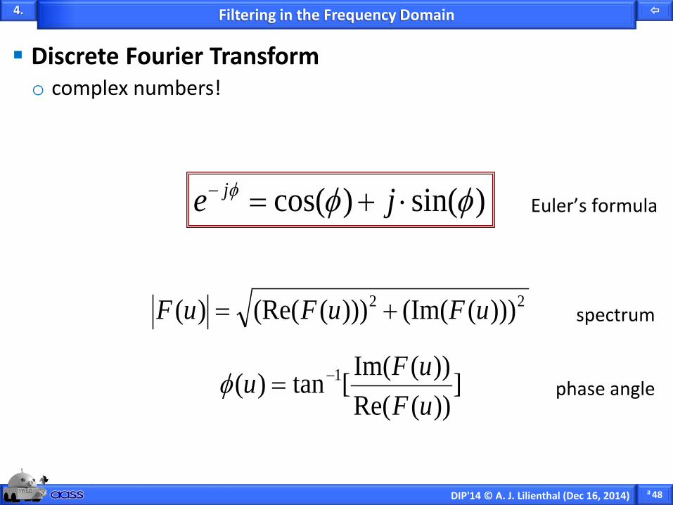
Discrete Fourier Transform o complex numbers!
Filtering in the Frequency Domain
Euler’s formula )sin()cos( φφφ ⋅+=− je j
22 )))((Im()))((Re()( uFuFuF +=
]))(Re())(Im([tan)( 1
uFuFu −=φ
spectrum
phase angle

# 49 DIP'14 © A. J. Lilienthal (Dec 16, 2014)
4.
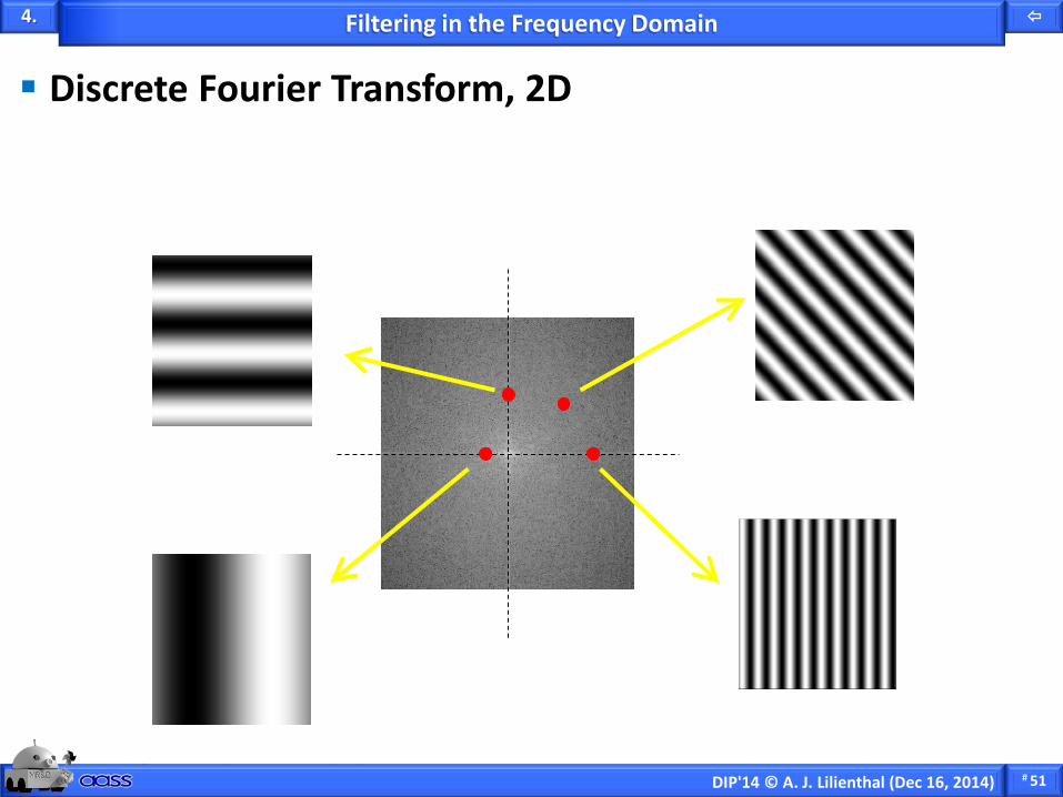
Discrete Fourier Transform, 2D
Filtering in the Frequency Domain
∑∑−
=
−
=
+−=1
0
1
0
)//(2),(1),(M
x
N
y
NvyMuxjeyxfMN
vuF π
1...,,1,0 −= Nv1...,,1,0 −= Mu

# 50 DIP'14 © A. J. Lilienthal (Dec 16, 2014)
4.
Discrete Fourier Transform, 2D
Filtering in the Frequency Domain
⋅ (-1)x+y
•F
log
→
c · log(1+|F(u,v)|)
# 51 DIP'14 © A. J. Lilienthal (Dec 16, 2014)
4.
Discrete Fourier Transform, 2D
Filtering in the Frequency Domain

# 52 DIP'14 © A. J. Lilienthal (Dec 16, 2014)
4.
Discrete Fourier Transform
Filtering in the Frequency Domain
Filtering in the Frequency Domain
Input Image ⋅ (-1)x+y F(u,v)
center the transform DFT
⋅ H(u,v)
apply filter
f(x,y)
inverse DFT
Re[f(x,y)]
Output Image
⋅ (-1)x+y

# 53 DIP'14 © A. J. Lilienthal (Dec 16, 2014)
4.
Discrete Fourier Transform
Filtering in the Frequency Domain o ideal low-pass, high-pass filters
» ringing
Filtering in the Frequency Domain

# 54 DIP'14 © A. J. Lilienthal (Dec 16, 2014)
4.
Understanding Questions o why does ringing occur?
Exam?

# 55 DIP'14 © A. J. Lilienthal (Dec 16, 2014)
4.
Discrete Fourier Transform
Filtering in the Frequency Domain o ideal low-pass, high-pass filters
» ringing o convolution theorem
Filtering in the Frequency Domain
),(),(),(),( vuHvuFyxhyxf ⋅⇔∗
),(),(),(),( vuHvuFyxhyxf ∗⇔⋅

# 56 DIP'14 © A. J. Lilienthal (Dec 16, 2014)
4.
Discrete Fourier Transform
Filtering in the Frequency Domain o ideal low-pass, high-pass filters
» ringing o convolution theorem
» link between spatial and frequency domain
» wrap around problem importance of padding
Filtering in the Frequency Domain
),(),( vuHyxh ⇔

# 57 DIP'14 © A. J. Lilienthal (Dec 16, 2014)
4.
Discrete Fourier Transform
Filtering in the Frequency Domain o ideal low-pass, high-pass filters
» ringing o convolution theorem
» link between spatial and frequency domain o Gaussian / Laplacian filter in the frequency domain
Filtering in the Frequency Domain
# 58 DIP'14 © A. J. Lilienthal (Dec 16, 2014)
4.
Discrete Fourier Transform
Filtering in the Frequency Domain
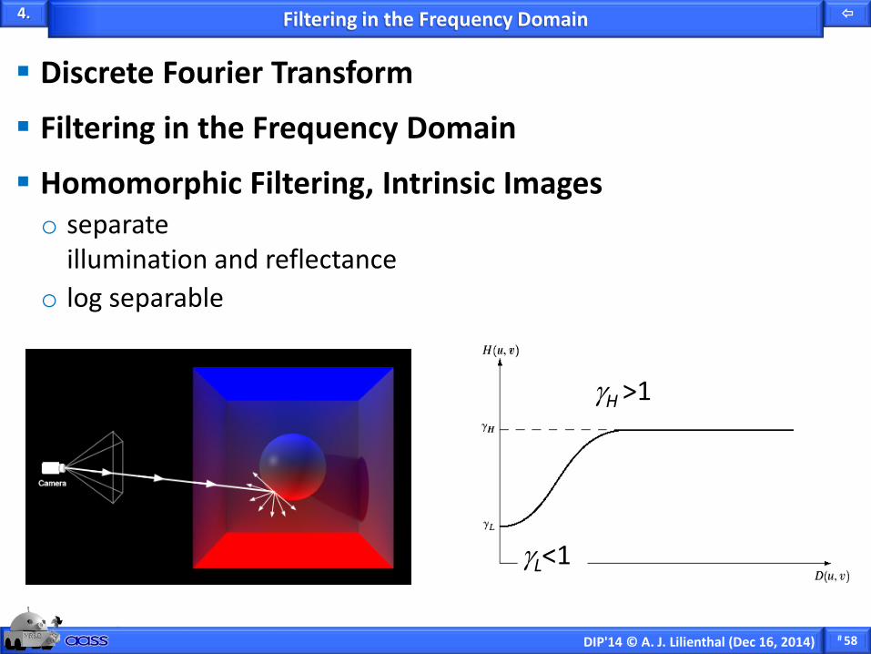
Homomorphic Filtering, Intrinsic Images o separate
illumination and reflectance o log separable
Filtering in the Frequency Domain
γL<1
γH >1
# 59 DIP'14 © A. J. Lilienthal (Dec 16, 2014)
4.
Discrete Fourier Transform
Filtering in the Frequency Domain
Homomorphic Filtering
Properties of the Fourier Transform o distributive? (over addition? over multiplication?) o scaling?, rotation?, ... o separability
Filtering in the Frequency Domain

# 62 DIP'14 © A. J. Lilienthal (Dec 16, 2014)
4.
Discrete Fourier Transform
Filtering in the Frequency Domain
Homomorphic Filtering
Properties of the Fourier Transform
Correlation, Template Matching
Filtering in the Frequency Domain
# 63 DIP'14 © A. J. Lilienthal (Dec 16, 2014)
4.
Discrete Fourier Transform
Filtering in the Frequency Domain
Homomorphic Filtering
Properties of the Fourier Transform
Correlation, Template Matching
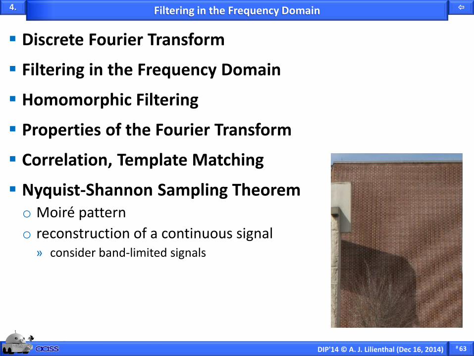
Nyquist-Shannon Sampling Theorem o Moiré pattern o reconstruction of a continuous signal
» consider band-limited signals
Filtering in the Frequency Domain

# 64 DIP'14 © A. J. Lilienthal (Dec 16, 2014)
4.
Discrete Fourier Transform
Filtering in the Frequency Domain
Homomorphic Filtering
Properties of the Fourier Transform
Correlation, Template Matching
Nyquist-Shannon Sampling Theorem o Moiré pattern o reconstruction of continuous signal
» consider band-limited signals
Filtering in the Frequency Domain
# 65 DIP'14 © A. J. Lilienthal (Dec 16, 2014)
4.
Discrete Fourier Transform
Filtering in the Frequency Domain
Homomorphic Filtering
Properties of the Fourier Transform
Correlation, Template Matching
Nyquist-Shannon Sampling Theorem
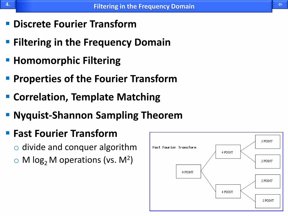
Fast Fourier Transform o divide and conquer algorithm o M log2 M operations (vs. M2)
Filtering in the Frequency Domain
# 66 DIP'14 © A. J. Lilienthal (Dec 16, 2014)
Part 5 – Image Restoration
5

# 67 DIP'14 © A. J. Lilienthal (Dec 16, 2014)
5.
Image Degradation and Restoration o model of the image degradation process
Image Restoration
Hdeg(x,y) f(x,y) +
n(x,y)
g(x,y)
# 69 DIP'14 © A. J. Lilienthal (Dec 16, 2014)
5.
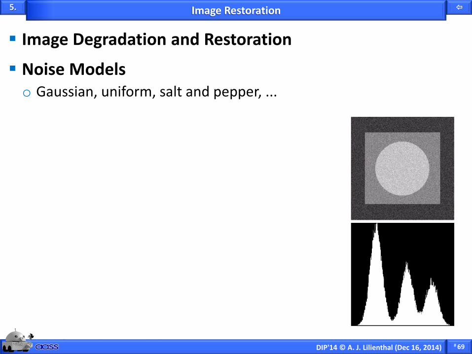
Image Degradation and Restoration
Noise Models o Gaussian, uniform, salt and pepper, ...
Image Restoration
# 70 DIP'14 © A. J. Lilienthal (Dec 16, 2014)
5.
Image Degradation and Restoration
Noise Models
Noise Reduction o assume additive noise
» uncorrelated with the image o estimation of noise shape and noise parameters
» by observation » by experimentation » by modelling
o apply appropriate filter (mean, median, adaptive mean, ...)
Image Restoration

# 71 DIP'14 © A. J. Lilienthal (Dec 16, 2014)
5.
Adaptive Mean Filter
o behaviour based on the local variance (σL average contrast) o if the noise has zero variance (σn = 0) then f(x,y)=g(x,y) o if the local variance σL is large compared to the noise variance σn then
f(x,y)≈g(x,y) → preserve edges
o if σL ≈ σn then f(x,y)≈mL (mean over the neighbourhood) → average out noise
Noise Reduction
( ) [ ]LL
n myxgyxgyxf −−= ),(),(,ˆ2
2
σσ
^
^
^

# 72 DIP'14 © A. J. Lilienthal (Dec 16, 2014)
5.
Image Degradation and Restoration
Noise Models
Noise Reduction o apply appropriate filter (notch filter)
» additive, periodic (approximately sinusoidal) noise
Image Restoration
F
→
# 73 DIP'14 © A. J. Lilienthal (Dec 16, 2014)
5.
Image Degradation and Restoration
Noise Models
Noise Reduction
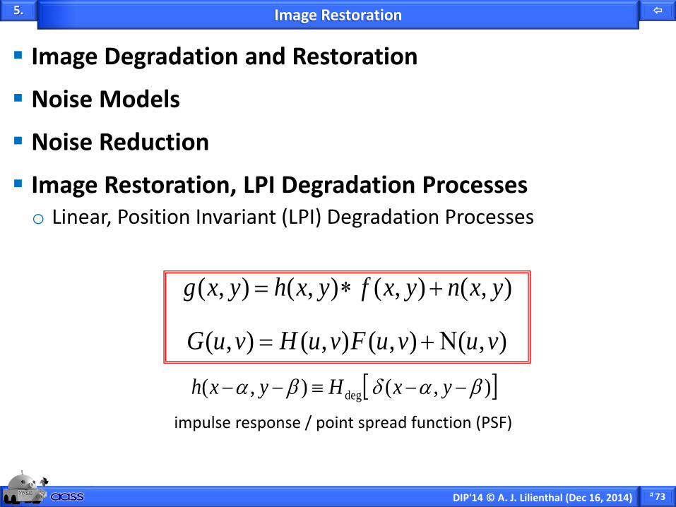
Image Restoration, LPI Degradation Processes o Linear, Position Invariant (LPI) Degradation Processes
Image Restoration
),(),(),(),( yxnyxfyxhyxg +∗=
),(),(),(),( vuvuFvuHvuG Ν+=
[ ]),(),( deg βαδβα −−≡−− yxHyxhimpulse response / point spread function (PSF)

# 74 DIP'14 © A. J. Lilienthal (Dec 16, 2014)
5.
Image Degradation and Restoration
Noise Models
Noise Reduction
Image Restoration, LPI Degradation Processes o Linear, Position Invariant (LPI) Degradation Processes o Inverse Filtering, Deconvolution
Image Restoration
),(),(),(
),(),(),(),(0),(
vuHvuGvuF
vuvuFvuHvuGvu
=⇔
Ν+==Ν
# 75 DIP'14 © A. J. Lilienthal (Dec 16, 2014)
5.
Image Degradation and Restoration
Noise Models
Noise Reduction
Image Restoration, LPI Degradation Processes o Linear, Position Invariant (LPI) Degradation Processes o Inverse Filtering, Deconvolution o estimating H
» by experimentation, image observation, modelling
Image Restoration

# 76 DIP'14 © A. J. Lilienthal (Dec 16, 2014)
5.
Image Degradation and Restoration
Noise Models
Noise Reduction
Image Restoration, LPI Degradation Processes o Linear, Position Invariant (LPI) Degradation Processes o Inverse Filtering, Deconvolution o estimating H
Wiener Filtering
Image Restoration
),(ˆ),(
),(/),(ˆ),(ˆ
),(ˆ),(ˆ
2
2
vuHvuG
vuSvuSvuH
vuHvuF
fn
+=

# 77 DIP'14 © A. J. Lilienthal (Dec 16, 2014)
5.
Image Degradation and Restoration
Noise Models
Noise Reduction
Image Restoration, LPI Degradation Processes o Linear, Position Invariant (LPI) Degradation Processes o Inverse Filtering, Deconvolution o estimating H
Wiener Filtering
Image Restoration
),(ˆ),(
),(ˆ
),(ˆ),(ˆ
2
2
vuHvuG
KvuH
vuHvuF
+=

# 78 DIP'14 © A. J. Lilienthal (Dec 16, 2014)
Part 6 – Colour Image Processing
6

# 79 DIP'14 © A. J. Lilienthal (Dec 16, 2014)
6.
Colour Fundamentals
Colour Image Processing
detector rods and cones

# 80 DIP'14 © A. J. Lilienthal (Dec 16, 2014)
6.
Colour Fundamentals o brightness, hue, saturation, chromaticity (hue+saturation)
Colour Image Processing

# 81 DIP'14 © A. J. Lilienthal (Dec 16, 2014)
6.
Colour Fundamentals
Colour Models o CIE
» colour perceived by a standard observer (gamut of human vision)
» tri-stimulus model
Colour Image Processing

# 82 DIP'14 © A. J. Lilienthal (Dec 16, 2014)
6.
Colour Fundamentals
Colour Models o CIE o RGB, CMYK
Colour Image Processing
# 83 DIP'14 © A. J. Lilienthal (Dec 16, 2014)
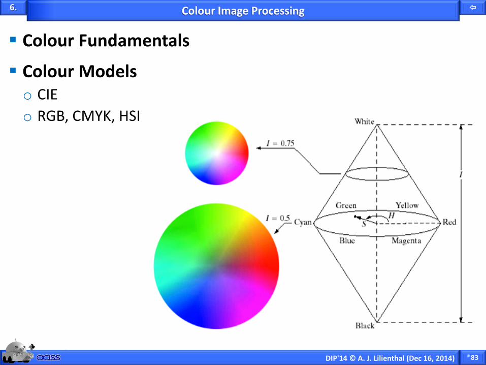
6.
Colour Fundamentals
Colour Models o CIE o RGB, CMYK, HSI
Colour Image Processing

# 85 DIP'14 © A. J. Lilienthal (Dec 16, 2014)
6.
Colour Fundamentals
Colour Models
Pseudo Color Processing
Colour Image Processing

# 86 DIP'14 © A. J. Lilienthal (Dec 16, 2014)
6.
Colour Fundamentals
Colour Models
Pseudo Color Processing
Colour Transformations o per-colour-component or vector transformation? o histogram equalization
» better in HSI or RGB?
Colour Image Processing
in
out
in
out
in
out
# 87 DIP'14 © A. J. Lilienthal (Dec 16, 2014)
6.
Colour Fundamentals
Colour Models
Pseudo Color Processing
Colour Transformations
Smoothing and Sharpening of Colour Images
Colour Image Processing

# 101 DIP'14 © A. J. Lilienthal (Dec 16, 2014)
Part 8 – Image Segmentation
8

# 102 DIP'14 © A. J. Lilienthal (Dec 16, 2014)
8.
Image Segmentation o in general a very difficult problem o full?, partial? o edge-based, region-based, motion-based
» idea: search for discontinuities and/or similarities in the image
Image Segmentation

# 103 DIP'14 © A. J. Lilienthal (Dec 16, 2014)
8.
Image Segmentation
Edge Detection o edge model
Image Segmentation

# 104 DIP'14 © A. J. Lilienthal (Dec 16, 2014)
8.
Image Segmentation
Edge Detection o edge model o edge detectors
» Prewitt, Sobel » Laplacian of a Gaussian
Image Segmentation

# 105 DIP'14 © A. J. Lilienthal (Dec 16, 2014)
8.
Image Segmentation
Edge Detection o edge model o edge detectors
» Prewitt, Sobel, Laplacian of a Gaussian » Canny edge detector
Image Segmentation

# 106 DIP'14 © A. J. Lilienthal (Dec 16, 2014)
8.
Image Segmentation
Edge Detection o edge model o edge detectors
» Prewitt, Sobel, Laplacian of a Gaussian » Canny edge detector
• noise reduction • edge enhancement • determination of the intensity gradient • non-maximum suppression • tracing edges through the image
• thresholds Thigh and Tlow
Image Segmentation
# 107 DIP'14 © A. J. Lilienthal (Dec 16, 2014)
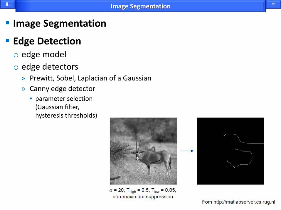
8.
Image Segmentation
Edge Detection o edge model o edge detectors
» Prewitt, Sobel, Laplacian of a Gaussian » Canny edge detector
• parameter selection (Gaussian filter, hysteresis thresholds)
Image Segmentation

# 108 DIP'14 © A. J. Lilienthal (Dec 16, 2014)
8.
Image Segmentation
Edge Detection o edge model o edge detectors
» Prewitt, Sobel, Laplacian of a Gaussian » Canny edge detector
o edge detection in colour Images
Image Segmentation
# 109 DIP'14 © A. J. Lilienthal (Dec 16, 2014)
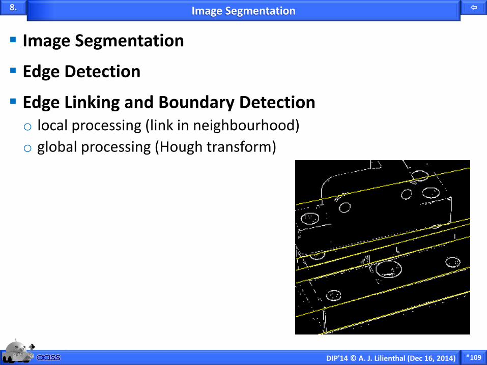
8.
Image Segmentation
Edge Detection
Edge Linking and Boundary Detection o local processing (link in neighbourhood) o global processing (Hough transform)
Image Segmentation
# 119 DIP'14 © A. J. Lilienthal (Dec 16, 2014)
Part 8 – Image Segmentation (Deep Questions)
8

# 120 DIP'14 © A. J. Lilienthal (Dec 16, 2014)
8.
What is Noise? What is Texture? o wet sand by Jay Sekora
Deep Questions

# 121 DIP'14 © A. J. Lilienthal (Dec 16, 2014)
8.
What is Noise? What is Texture? o human skin by Ken Perlin
Deep Questions

# 122 DIP'14 © A. J. Lilienthal (Dec 16, 2014)
8.
What is an Edge in Human Vision? o illusory contours by G. Kanizsa (1955)
Deep Questions

# 123 DIP'14 © A. J. Lilienthal (Dec 16, 2014)
8.
Does Absolute Intensity Matter? o often perceived intensity ≠ pixel values
o center strip has constant intensity
Deep Questions
# 124 DIP'14 © A. J. Lilienthal (Dec 16, 2014)
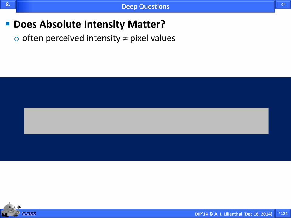
8.
Does Absolute Intensity Matter? o often perceived intensity ≠ pixel values
o center strip has constant intensity
Deep Questions

# 125 DIP'14 © A. J. Lilienthal (Dec 16, 2014)
8.
What is an Illumination Edge? o sometimes it isn’t a large intensity change …
Deep Questions

# 126 DIP'14 © A. J. Lilienthal (Dec 16, 2014)
8.
What is a Geometric Edge in Images? o some silhouettes are
suggested by shape cues » 3D "peanut" shape
Deep Questions

# 127 DIP'14 © A. J. Lilienthal (Dec 16, 2014)
8.
What Is an Edge at The Finest Scales? o scale problems:
can’t resolve every hair and fiber in fur » Albrecht Dürer (1502)
Deep Questions

# 128 DIP'14 © A. J. Lilienthal (Dec 16, 2014)
8.
Very Difficult Images o edge? o noise? o regions? o texture? o silhouette? o …
Deep Questions

Mobile Robotics and Olfaction Lab, AASS, Örebro University
# 150
Achim J. Lilienthal
Room T1227, Mo, 11-12 o'clock (please drop me an email in advance)


