
Mining at scale with latent factor
models for matrix completion
Fabio Petroni
Sapienza University of Rome, 2015


Mining at scale with latent factor
models for matrix completion
Fabio Petroni
Ph.D. program in Engineering in Computer Science.
Department of Computer, Control, and Management
Engineering Antonio Ruberti
at Sapienza University of Rome
presented by
Fabio Petroni
Rome, 02/02/2016

Author:
Fabio Petroni
http://www.fabiopetroni.com
Thesis Committee:
Prof. Aris Anagnostopoulos
Prof. Leonardo Querzoni (Advisor)
Reviewers:
Prof. Irwin King
Prof. Sebastian Riedel
Contents
Sommario vi
Abstract ix
1 Introduction 1
1.1 Contributions . . . . . . . . . . . . . . . . . . . . . . 8
2 Matrix Completion 13
2.1 Recommender Systems . . . . . . . . . . . . . . . . . 14
2.1.1 Collaborative Filtering . . . . . . . . . . . . . 15
2.2 The Matrix Completion Problem . . . . . . . . . . . 19
2.3 Latent Factor Models . . . . . . . . . . . . . . . . . . 20
2.4 Optimization Criteria . . . . . . . . . . . . . . . . . . 22
2.4.1 Regularized Squared Loss . . . . . . . . . . . 23
2.4.2 Bayesian Personalized Ranking . . . . . . . . 24
2.5 Stochastic Gradient Descent . . . . . . . . . . . . . . 26
2.6 Summary . . . . . . . . . . . . . . . . . . . . . . . . 28
vi CONTENTS
3 Distributed Matrix Completion 31
3.1 Distributed Stochastic Gradient Descend . . . . . . . 33
3.1.1 Stratified SGD . . . . . . . . . . . . . . . . . 34
3.1.2 Asynchronous SGD . . . . . . . . . . . . . . . 35
3.2 Input Partitioner . . . . . . . . . . . . . . . . . . . . 39
3.2.1 Problem Definition . . . . . . . . . . . . . . . 40
3.2.2 Streaming Algorithms . . . . . . . . . . . . . 43
3.2.3 The HDRF Algorithm . . . . . . . . . . . . . 46
3.2.4 Theoretical Analysis . . . . . . . . . . . . . . 50
3.3 Evaluation . . . . . . . . . . . . . . . . . . . . . . . . 54
3.3.1 Experimental Settings and Test Datasets . . . 54
3.3.2 Performance Evaluation . . . . . . . . . . . . 59
3.4 Summary . . . . . . . . . . . . . . . . . . . . . . . . 72
4 Context-Aware Matrix Completion 75
4.1 Context-Aware Algorithms . . . . . . . . . . . . . . . 76
4.2 Open Relation Extraction . . . . . . . . . . . . . . . 78
4.2.1 Relation Extraction Algorithms . . . . . . . . 79
4.3 Context-Aware Open Relation Extraction . . . . . . 83
4.3.1 The CORE Model . . . . . . . . . . . . . . . 85
4.4 Evaluation . . . . . . . . . . . . . . . . . . . . . . . . 93
4.4.1 Experimental Setup . . . . . . . . . . . . . . . 93
4.4.2 Results . . . . . . . . . . . . . . . . . . . . . . 97
4.5 Summary . . . . . . . . . . . . . . . . . . . . . . . . 101

Contents vii
5 Conclusion and Outlook 103
5.1 Future Work . . . . . . . . . . . . . . . . . . . . . . . 106
5.1.1 Improvements . . . . . . . . . . . . . . . . . . 106
5.1.2 Open research problems . . . . . . . . . . . . 107

viii Sommario

Sommario
Predire quali relazioni e probabile che si verifichino tra oggetti del
mondo reale e un compito fondamentale per diverse applicazioni. Ad
esempio, i sistemi di raccomandazione automatici mirano a predire
l’esistenza di relazioni sconosciute tra utenti e oggetti, e sfruttano
tali informazioni per fornire suggerimenti personalizzati di oggetti
potenzialmente d’interesse per uno specifico utente. Le tecniche di
completamento di matrice mirano a risolvere questo compito, in-
dentificando e sfruttando i fattori latenti che hanno innescato la
creazione di relazioni note, al fine di dedurre quelle mancanti.
Questo problema, tuttavia, e reso difficile dalle dimensioni dei data-
set odierni. Un modo per gestire tale mole di dati, in un ragionevole
lasso di tempo, e quello di distribuire la procedura di completamento
della matrice su un cluster di macchine. Tuttavia, gli approcci cor-
renti mancano di efficienza e scalabilita, poiche, per esempio, non
minimizzano la comunicazione o garantiscono un carico di lavoro
equilibrato nel cluster.

x Sommario
Un ulteriore aspetto delle tecniche di completamento di matrice pre-
so in esame e come migliorare la loro capacita predittiva. Questo puo
essere fatto, per esempio, considerando il contesto in cui le relazioni
vengono catturate. Tuttavia, incorporare informazioni contestuali
generiche all’interno di un algoritmo di completamento matrice e un
compito difficile.
Nella prima parte di questa tesi vengono studiate soluzioni distri-
buite per il completamento della matrice e affrontate le questioni di
cui sopra esaminando tecniche di suddivisione dell’input, basate su
algoritmi di partizionamento di grafi. Nella seconda parte della tesi
ci si concentra su tecniche di completamento di matrice consapevo-
li del contesto, fornendo soluzioni che possono essere applicate sia
(i) quando le voci note nella matrice assumono piu valori e sia (ii)
quando assumono tutte lo stesso valore.

Abstract
Predicting which relationships are likely to occur between real-world
objects is a key task for several applications. For instance, recom-
mender systems aim at predicting the existence of unknown rela-
tionships between users and items, and exploit this information to
provide personalized suggestions for items to be of use to a specific
user. Matrix completion techniques aim at solving this task, identi-
fying and leveraging the latent factors that triggered the the creation
of known relationships to infer missing ones.
This problem, however, is made challenging by the size of today’s
datasets. One way to handle such large-scale data, in a reasonable
amount of time, is to distribute the matrix completion procedure
over a cluster of commodity machines. However, current approaches
lack of efficiency and scalability, since, for instance, they do not
minimize the communication or ensure a balance workload in the
cluster.
xii Abstract
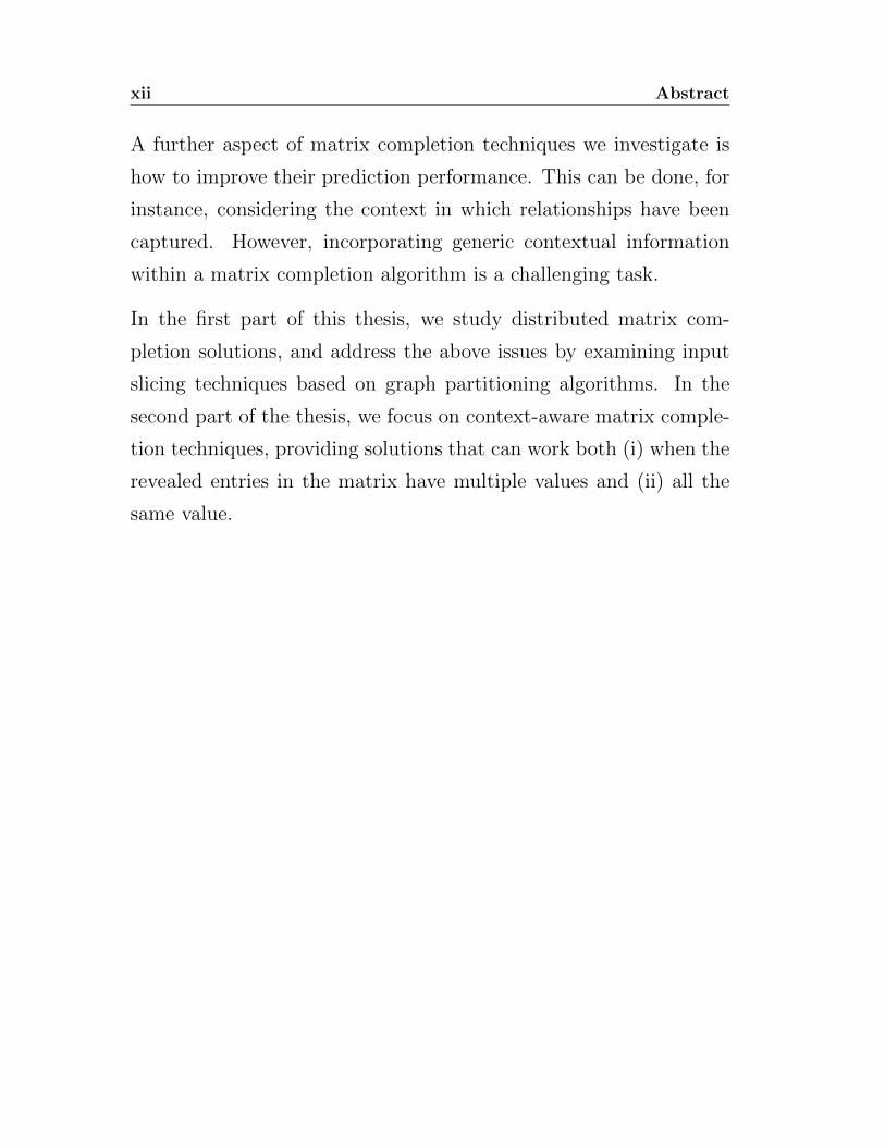
A further aspect of matrix completion techniques we investigate is
how to improve their prediction performance. This can be done, for
instance, considering the context in which relationships have been
captured. However, incorporating generic contextual information
within a matrix completion algorithm is a challenging task.
In the first part of this thesis, we study distributed matrix com-
pletion solutions, and address the above issues by examining input
slicing techniques based on graph partitioning algorithms. In the
second part of the thesis, we focus on context-aware matrix comple-
tion techniques, providing solutions that can work both (i) when the
revealed entries in the matrix have multiple values and (ii) all the
same value.

CHAPTER 1
Introduction
The Web, they say, is leaving the era of search and
entering one of discovery. What’s the difference? Search
is what you do when you’re looking for something.
Discovery is when something wonderful that you didn’t
know existed, or didn’t know how to ask for, finds you.
Jeffrey M. O’Brien
Understanding the underlying causes that lead to the creation of
relationships among objects is a crucial task to acquire a deeper
knowledge of the world, and predict its evolution. While some rela-
tionships are relatively easy to capture and model, others, although
present in the world, are by their nature difficult to represent, es-
pecially when their interpretation is hidden inside large amounts of
data. The study of such relationships is essential in several scientific

2 1. Introduction
fields, ranging from biology to sociology, from physics to engineer-
ing, and its exploitation has led to several important advances in
recent years. For instance, recent techniques for mineral exploration
avoid deep holes to look for regions containing desirable materials,
but just analyze samples near the surface [25]. By understanding the
relationships among deeply buried mineral deposit and near-surface
geochemistry it is possible to predict the location of the former with-
out drilling, therefore minimizing the environmental impact. Simi-
larly, the relationships between users in online social networks, which
drastically changed the way people interact and communicate, are a
rich source of information for computer and social sciences, but also
for commercial purposes. For instance, by understanding the fac-
tors that led to two users to be friends, it is possible to predict and
suggest other users with whom they might be interested to connect
[77].
The current data production rate, however, poses additional chal-
lenges to the task of understanding and modeling such relationships.
The last few years, in particular, have witnessed a huge growth in
information production. Some corporations like IBM estimate that
“2.5 quintillion bytes of data are created every day”, amounting
to 90% of the data in the world today having been created in the
last two years [37]. For this reason, legacy approaches, based, for
instance, on manual inspection, are being rapidly replaced by auto-
matic data mining methods based on machine learning techniques,
able to cope with data at such massive scale and to produce far
better results. The term “data mining”, indeed, derives from the
metaphor of data as something that is very large, contains far too
3
much information to be used, but can be mined to extract nuggets
of valuable knowledge.
One successful approach to represent relationships, whose interpre-
tation is hidden inside large scale dataset, is to model the objects as
points in a d dimensional space. The dimensions of such space rep-
resent latent factors that originate the relationships. Each object is
therefore modeled as a vector of real values, one for each considered
latent factor. For instance, consider a person that likes the band
Sex Pistols. A possible explanation for this “like” relationship is
that the musical tastes of the person are geared toward punk music
(factor one) and that he has a rebel character (factor two). Such
explanation can be represented in a two-dimensional space, where
dimensions correspond to the factor punk music and the factor rebel
character. A two-dimensional vector is associated with both the user
and the band, with and high value for the two factors, i.e., they lie
close in the latent factor space. These factors are called “latent” be-
cause they are not directly observable in the data. Moreover, unlike
this example, in real applications (1) it is often impossible to provide
a clear interpretation for them and (2) the number of considered la-
tent factors is much higher. By comparing the latent representations
of different objects it is possible to derive the existence of unknown
relationships among them. For instance, the system might predict
that the above person also likes the band Ramones, since also this
object has a vector representation with an high value for the two
considered latent factors.
In this thesis we restrict our focus to binary relationships, that can
be represented in the form of a matrix, where rows and columns rep-

4 1. Introduction
resent objects, and entries report the interactions among them. For
example, a matrix might represent friendship relationships between
users in an online social network. In this case, rows and columns
represent users and an entry equal to one indicates that the row
user and the column user are friends. In many practical problems of
interest, only a (usually really small) portion of entries in the data
matrix are known. By leveraging the latent vector representation
of objects is possible to complete the missing part of the matrix,
adding new entries as coherent as possible with the observed data.
For the sake of clarity, consider the following two scenarios, where
such kind of matrix completion techniques have been successfully
applied, as prototypical applications.
Collaborative Filtering in Recommender Systems. A recom-
mender system collects the preferences that a set of users express on
a set of items and, by exploiting this information, tries to provide
personalized recommendations that fit the users’ personal tastes.
Several e-commerce leaders, like Amazon.com, Pandora and Net-
flix, have made recommender systems a crucial cornerstone of their
data management infrastructure to boost their business offerings. In
the last two decades, a consistent research effort has been devoted to
the task of developing algorithms able to generate recommendations.
The resulting research progress has established collaborative filter-
ing (CF) techniques as the dominant framework for recommender
systems [1, 121, 39, 103, 63]. Such methods look at the ratings of
like-minded users to provide recommendations, with the idea that
users who have expressed similar interests in the past will share
common interests in the future. A large bunch of machine learn-

5
ing techniques have been exploited for collaborative filtering (see
section 2.1.1). Among this multitude of algorithms, matrix comple-
tion techniques based on latent factor models have emerged as the
best approach to collaborative filtering, due to their advantages with
respect to both scalability and accuracy [123, 66, 73, 91]. The as-
sumption behind such solutions is that only a few factors contribute
to an individual’s tastes or preferences. The data matrix in this
case is composed with users as rows, item as columns and ratings
as entries. By completing this matrix is possible to infer users’ pref-
erences for unrated items, and exploit these predictions to provide
personalized recommendations.
Open Relation Extraction in Natural Language Processing.
Relation extraction is concerned with predicting the existence of
unknown relations (e.g., “was born in”) among real word entities
(e.g., persons, locations, organizations). These systems take in input
a set of real word facts, expressed as relation-subject-object triples,
and correlate them to estimate the likelihood of unobserved facts.
For example, a relation extraction system may be fed with facts
such as “is the singer of”(“Thom Yorke”, “Radiohead”), “is band
member of”(“Ringo Starr”, “The Beatles”), etc. Several machine
learning methods have been leveraged for relation extraction (see
section 4.2.1); they can be broadly classified in closed and open
approaches. Closed approaches [80, 86, 22] aim at predicting new
facts for a predefined set of relations, usually taken from an existing
knowledge base. Open relation extraction techniques [104, 30, 90],
instead, aim at predicting new facts for a potentially unbounded
set of relations, which come from various sources, such as natural

6 1. Introduction
language text and knowledge bases. One of the most successful
techniques for open relation extraction is based on matrix completion
[104, 90]. The corresponding data matrix is usually represented with
relations as columns and subject-object pairs as rows; an entry equal
to one means that a fact has been observed in input referring to the
subject-object pair (in the row) and the relation (in the column).
By completing the matrix it is possible to estimate the likelihood of
each unobserved fact, associated with a missing entry in the data
matrix, and to exploit this information to predict new facts. In the
above example, for instance, the system might predict the fact “is
band member of”(“Thom Yorke”, “Radiohead”).
The above application scenarios have some peculiar characteristics
and difficulties; for instance, one fundamental difference between the
two is that in recommender systems users can usually provide both
positive and negative feedback (e.g., on a zero-to-five scale) while a
fact in natural language is either observed or not, i.e., there are only
positive observations in input and no explicit negative evidence. The
data matrix reflects these two scenarios, in that revealed entries have
multiple values in the former case, all the same value in the latter
case. This leads to two different ways to learn latent factor models
able to complete the matrix.
One common characteristics of the above scenarios, and of general
instances of the matrix completion problem, is that real applica-
tions may involve millions of objects and billions of entries in the
matrix; for instance, Amazon.com offers thousands of products to
more than 200M active customers, and, only in 2014, the number
of purchases was estimated around 2B [120]. The amount of data
7
available for such kind of systems is indeed a key factor for their
effectiveness [49]. In order to cope with datasets at such massive
scales, in a reasonable amount of time, parallel and distributed ap-
proaches are essential. Here we consider a general shared-nothing
distributed architecture which allows asynchronous communication
between computing nodes. The main challenges in this environment
are concerned with the partitioning of the data matrix among the
computing nodes; the goal is to distribute the data so that (1) each
computing nodes operates on subsets of the data with minimum
overlap with each other, in order to minimize the communication
and (2) the workload is fairly balanced among nodes to maximize
the efficiency. However, current solutions only partially solve the
above challenges, in that they use simple or general purpose parti-
tioning algorithms. For example, these techniques do not take into
consideration common characteristics of the input data that can help
in optimizing the data placement over the two aforementioned lines,
as, for instance, the relationships power-law distribution, often vis-
ible in real data, i.e., most objects have relatively few relationships
(e.g., niche movies rated by few) while a few have many (e.g., pop-
ular movies rated by many).
The overall performance of matrix completion solutions can be boosted
not only feeding the system with more data [49], but also integrat-
ing contextual information in the model [90]. To have some insights
on the economic value that a performance improvement in such sys-
tems can generate, consider that Netflix awarded a 10% boost in
prediction accuracy for its recommendation system with $1M via
the widely-publicized Netflix prize [12]. In many application do-
8 1. Introduction
mains, a context-agnostic approach to matrix completion may lose
predictive power because potentially useful information from mul-
tiple contexts is aggregated. Even human understanding often re-
quires the use of context. For example, the natural language relation
“plays with”(x,y) is unspecific, possible meanings include play sports
or play in a band. However, the comprehension can be facilitated
if contextual information is available, for instance the topic of the
document where the relation is extracted (e.g., sport, music, etc.).
The integration of generic contextual information within a matrix
completion model is a relatively new line of research [2, 96, 97, 114];
some solutions have been proposed, mainly focused on collabora-
tive filtering in recommender systems (see section 4.1). An open
challenge in this domain is how to incorporate such contextual data
when the system is fed only with positive feedback, that is when the
revealed entries in the matrix have all the same value.
1.1 Contributions
This thesis deals with the aforementioned challenges, and provides
scalable solutions for matrix completion, as well as efficient ways
to integrate contextual information in the predictive model, even in
those cases when the revealed entries in the matrix have all the same
value (i.e., there is no negative evidence in input). Our contributions
can be summarized as follows.
1.1 Contributions 9
Distributed Matrix Completion.
We investigated distributed matrix completion solutions, able to per-
form the training procedure over a shared noting cluster of com-
puting nodes, using as application scenario collaborative filtering
in recommender systems. We review existing centralized, parallel
(i.e., working on shared memory) and distributed approaches based
on stochastic gradient descent, a popular technique used to learn
the latent factor representations for the objects. We focus on asyn-
chronous version of the stochastic gradient descend algorithm for
large-scale matrix completion problems, and we propose a novel vari-
ant, namely GASGD, that leverages data partitioning schemes based
on graph partitioning techniques and exploits specific characteristics
of the input data to tackle the above challenges, that is to reduce
the communication among computing nodes while maintaining the
load balanced in the system. This approach looks at the input data
as a graph where each vertex represents an object (i.e., either a row
or a column) and each edge represents a relationship between the
two vertices (i.e, an entry in the data matrix).
To partition the input data, we considered several state-of-the-art
graph partitioning algorithms that consume the input data in a
streaming fashion, thus imposing a negligible overhead to the over-
all execution time. However, existing graph partitioning solutions
only partially exploit the skewed power-law degree distribution of
real world dataset. To fill this gap, we propose high degree (are)
replicated first (HDRF ), a novel stream-based graph partitioning
algorithm based on a greedy vertex-cut approach that effectively ex-
ploits skewed degree distributions by explicitly taking into account
10 1. Introduction
vertex degree in the placement decision. HDRF is characterized by
the following desirable properties: (1) it outputs a partition with
the smallest average replication factor among all competing solu-
tions and (2) it provides close to optimal load balancing, even in
those cases where classic greedy approaches typically fail. On the
one hand, lowering the average replication factor is important to
reduce network bandwidth cost, memory usage and replica synchro-
nization overhead at computation time. A fair distribution of load
in the partition, on the other hand, allows a more efficient usage
of available computing resources. Both aspects, when put together,
can positively impact the time needed to execute matrix completion
and, in general, graph computation algorithms. Our experimental
evaluation, conducted on popular real-word datasets, confirm that
HDRF combines both these aspects; matrix completion algorithms
run up to two times faster using HDRF as input partitioner with
respect to state-of-the-art partitioning algorithms. We also report a
theoretical analysis of the HDRF algorithm, and provide an upper
bound for the replication factor.
Context-Aware Matrix Completion. We study context aware
matrix completion solutions, able to incorporate generic contextual
information within the predictive model. We review existing ap-
proaches, mainly proposed for collaborative filtering, that work with
a matrix in which revealed entries have multiple values, that is when
the system is fed with both positive and negative evidence. We
proposed a novel algorithm to incorporate contextual data even in
those cases in which the revealed entries in the matrix have all the
same value, using as application scenario relation extraction, a pop-

1.1 Contributions 11
ular natural language processing task. In particular, we propose
CORE, a novel matrix completion model that leverages contextual
information for open relation extraction. Our model integrates facts
from various sources, such as natural language text and knowledge
bases, as well as the context in which these facts have been observed.
CORE employs a novel matrix completion model that extends ex-
isting context-aware solutions so as to work in those situations in
which the system receive in input only positive feedback (i.e., ob-
served facts). Our model is extensible, i.e., additional contextual
information can be integrated when available. We conducted an ex-
perimental study on a real-world dataset; even with limited amount
of contextual information used, our CORE model provided higher
prediction performance than previous solutions.

12 1. Introduction

CHAPTER 2
Matrix Completion
Essentially, all models are wrong, but some are useful.
George E. P. Box
Matrix completion is at its heart a technique to reconstruct a matrix
for which only a small portion of entries are available. This task is re-
lated with general matrix factorization models, such as matrix recon-
struction or non-negative matrix factorization [119]. In those cases,
however, all entries in the matrix are available and need to be taken
into consideration, and computing a low-rank model is relatively
easy (e.g., through singular value decomposition [13, 108]). Matrix
completion is, instead, impossible without additional assumptions,
and, even with those, the problem is not only NP-hard, but all known
algorithms require time doubly exponential in the dimension of the
matrix [24, 21].

14 2. Matrix Completion
Approximated matrix completion methods have been proposed to
reduce the computational cost of exact solutions, and, therefore, to
be of practical interest. Such techniques are currently experiencing
a growing interest in several fields of the data mining and machine
learning community, driven by the enormous success they achieve in
recommender systems, an application scenario that we will use as
baseline for exposition.
2.1 Recommender Systems
For users today’s world wide web it’s the tyranny of choice. Consider
that people on average read around ten megabytes (MB) worth of
material a day; hear 400MB a day, and see one MB of information
every second [38]. However, every 60 seconds 1500 blog entries are
created, 98000 tweets are shared, and 600+ videos are uploaded
to YouTube [84]. Studies have repeatedly shown that when people
are confronted with too many choices their ability to make rational
decisions declines [110]. Recommender systems aims at reducing
such choices and make the life of the users easier.
Many of todays internet businesses strongly base their success in
the ability to provide personalized user experiences. This trend,
pioneered by e-commerce companies like Amazon [75], has spread
to many different sectors. As of today, personalized user recom-
mendations are commonly offered by internet radio services (e.g.,
Pandora Internet Radio), social networks (e.g., Facebook), media
sharing platforms (e.g., YouTube) and movie rental services (e.g.,
Netflix). To estimate the economic value of such recommendations,
2.1 Recommender Systems 15
consider that 2/3 of the movies watched on Netflix are recommended,
recommendations generate 38% more clickthrough in Google news
and 35% sales in Amazon came from recommendations [6]. In gen-
eral, personalization techniques are considered the lifeblood of the
social web [106].
A widely adopted approach to build recommendation engines is rep-
resented by collaborative filtering algorithms.
2.1.1 Collaborative Filtering
Collaborative filtering (CF) is a thriving subfield of machine learn-
ing, and several surveys expose the achievements in this fields [1,
121, 39, 103, 63]. The essence of CF lies in analyzing the known
preferences of a group of users to make predictions of the unknown
preferences for other users.
The first work on the field of CF was the Tapestry system [46], de-
veloped at Xerox PARC, that used a manual collaborative filtering
system to filter mails, using textual queries, based on the opinion
of other users, expressed with simple annotations (such as “use-
ful survey” or “excellent”). Shortly after, the GroupLens system
[102, 62] was developed, a pioneer application that gave users the
opportunity to rate articles on a 1 to 5 scale and receive automatic
suggestions. Quickly recommender systems and collaborative filter-
ing became a hot topic in several research communities, ranging
from machine learning to human–computer interaction, and a large
number of algorithms started to be proposed. Moreover, in the same
period, commercial deployments of recommender systems, pioneered

16 2. Matrix Completion
SVD PMFuser based PLS(A/I)
memory based
collaborative filtering
item based
model based
probabilistic methods
neighborhood models
dimensionality reduction
matrix completion
latent Dirichlet allocation
other machine learning methods
Bayesian networks
Markov decision processes
neural networks
Figure 2.1: Taxonomy of collaborative filtering algorithms.
by companies such as Amazon.com, Yahoo! and Netflix, began to
spread all over the world wide web. The effort of the community
in this field experienced a significant boost in 2006, when Netflix
launched a competition to improve their recommendation engine:
the Netflix prize [12]. The objective of this open competition was to
build a recommender algorithm that could improve the internal Net-
flix solution on a fixed dataset by 10%. The reward for the winner
was US$1,000,000, an amount that demonstrate the importance of
accurate recommendations for vendors. The Netflix prize triggered
a feverish activity, both in academia and among hobbyists, that led
to several advances and novel solutions.
It is possible to divide existing CF techniques in two main groups:
memory-based and model-based [19, 1, 39] (see figure 2.1).
Memory-based algorithms operate on the entire database of ratings
to compute similarities between users or items. Such similarities con-
stitute the “memory” of the collaborative filtering system, and are
successively exploited to produce recommendations. Similar users
or items are identified using a similarity metric, such as the Pearson
2.1 Recommender Systems 17
correlation coefficient [102] and the cosine similarity [10, 118], that
analyzes and compares the rating vectors of either users or items.
The basic idea is to generate predictions by looking at the ratings of
the most similar users or items; for this reason such techniques are
called neighborhood models.
Neighborhood models are categorized as user based or item based.
User based methods compute a similarity score between each pair of
users, and then estimate unknown ratings based on recorded ratings
of similar users [51, 133, 113]. Item-oriented methods, instead, use
the known ratings to compute similarities between items, and then
provide recommendations by looking at similar items to those that
an user has previously rated [109, 68, 33].
Memory-based methods are used in a lot of real-world systems be-
cause of their simple design and implementation. However, they
impose several scalability limitations, since the computation of simi-
larities between all pairs of users or items is expensive (i.e., quadratic
time complexity with respect to the number of users or items), that
makes their use impractical when dealing with large amounts of data.
Model-based approaches have been investigated to overcome the short-
comings of memory-based algorithms. They use the collection of
ratings to estimate or learn a model and then apply this model to
make rating predictions. A large amount of machine learning tech-
niques have been used to build such model. In this multitude of
algorithms, a noteworthy families of solutions are dimensionality re-
duction techniques.
The idea behind such solutions is to reduce the dimensionality of
the rating space, in order to discover underlying structures that can

18 2. Matrix Completion
be leveraged to predict missing ratings. Traditional collaborative
filtering solutions, in fact, view the user-item ratings domain as a
vector space, where a vector with an entry for each user is associated
to each item, and vice-versa. These solutions aims at reducing the
dimensionality of such vectors, and therefore of the domain space, to
some fixed constant number d, so that both users and items can be
represented as a d-dimensional vector. The underlying assumption is
that the interaction between users and items (i.e., the ratings) can be
modeled using just d factors. Such factors can be modeled explicitly,
i.e., topics of interest, or can be considered latent in the ratings
data. Latent representation of users and items can be extracted
using singular value decomposition (SVD) [13, 108], a technique that
decompose the rating matrix in three constituent matrices of smaller
size, and exploit the factorization of them to predict missing ratings.
However, SVD-based models can be applied only when the input
matrix is complete. Since the rating matrix contains, by its nature,
a large portion of missing values, some heuristics must be applied
to pre-fill missing values; examples include, use the item’s average
rating or consider missing values as zeros.
Matrix completion techniques [64, 66, 123] avoid the necessity of
pre-filling missing entries by reasoning only on the observed ratings.
They can be seen as an estimate or an approximation of the SVD,
computed using application specific optimization criteria. Such so-
lutions are currently considered as the best single-model approach
to collaborative filtering, as demonstrated, for instance, by several
public competitions, such as the Netflix prize [12] and the KDD-Cup
2011 [35], and they will be extensively described in the rest of this
2.2 The Matrix Completion Problem 19
thesis.
Another remarkable families of collaborative filtering solutions are
probabilistic methods, that use statistical probability theory rather
than linear algebra to predict missing ratings. Example of such
methods include probabilistic matrix factorization (PMF) [81, 71],
probabilistic latent semantic analysis/indexing (PLSA/I) [52, 56, 29]
and latent Dirichlet allocation [14]. Other machine learning tech-
niques for collaborative filtering include Markov decision processes
[111], Bayesian networks [19, 137], and neural networks [105]. The
main advantage of dimensionality reduction techniques over other
existing solution is the availability of efficient parallel and distributed
implementations, that make it possible to handle very large-scale in-
stances of the problem, in a reasonable amount of time.
2.2 The Matrix Completion Problem
We consider a system constituted by U = (u1, · · · , un) users and
X = (x1, · · · , xm) items. Items represent a general abstraction that
can be case by case instantiated as news, tweets, shopping items,
movies, songs, etc. Users can either explicitly express their opinion
by rating items with values from a predefined range (i.e., explicit
feedback) or just provide an implicit indication of their taste (i.e.,
implicit feedback), for instance by clicking on a website. Without
loss of generality, here we assume that ratings are represented with
real numbers. By collecting user ratings it is possible to build a n×mrating matrix R that is usually a sparse matrix as each user rates
a small subset of the available items. Denote by O ⊆ {1, ..., n} ×
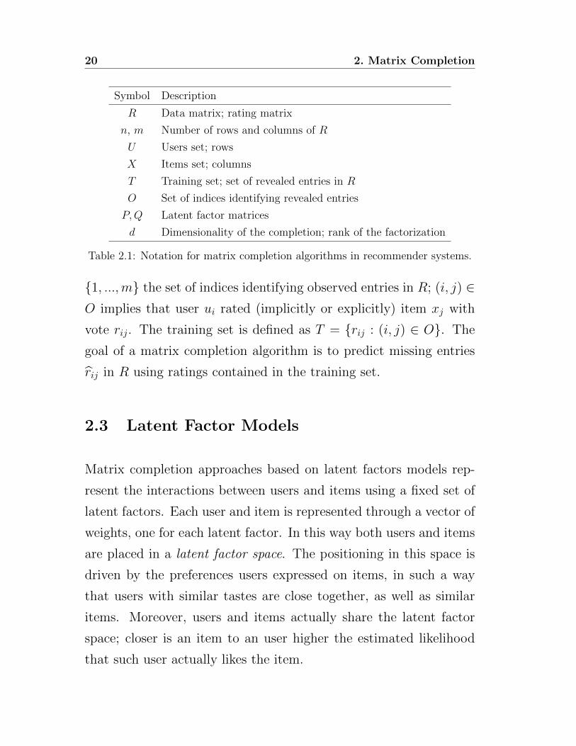
20 2. Matrix Completion
Symbol Description
R Data matrix; rating matrix
n, m Number of rows and columns of R
U Users set; rows
X Items set; columns
T Training set; set of revealed entries in R
O Set of indices identifying revealed entries
P,Q Latent factor matrices
d Dimensionality of the completion; rank of the factorization
Table 2.1: Notation for matrix completion algorithms in recommender systems.
{1, ...,m} the set of indices identifying observed entries in R; (i, j) ∈O implies that user ui rated (implicitly or explicitly) item xj with
vote rij. The training set is defined as T = {rij : (i, j) ∈ O}. The
goal of a matrix completion algorithm is to predict missing entries
rij in R using ratings contained in the training set.
2.3 Latent Factor Models
Matrix completion approaches based on latent factors models rep-
resent the interactions between users and items using a fixed set of
latent factors. Each user and item is represented through a vector of
weights, one for each latent factor. In this way both users and items
are placed in a latent factor space. The positioning in this space is
driven by the preferences users expressed on items, in such a way
that users with similar tastes are close together, as well as similar
items. Moreover, users and items actually share the latent factor
space; closer is an item to an user higher the estimated likelihood
that such user actually likes the item.
2.3 Latent Factor Models 21
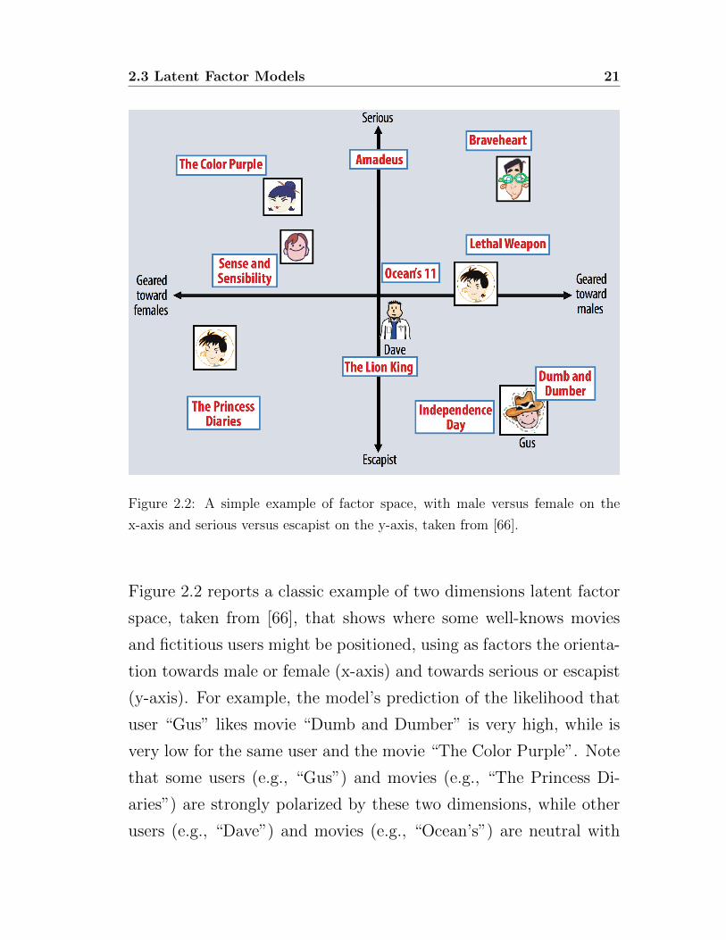
Figure 2.2: A simple example of factor space, with male versus female on the
x-axis and serious versus escapist on the y-axis, taken from [66].
Figure 2.2 reports a classic example of two dimensions latent factor
space, taken from [66], that shows where some well-knows movies
and fictitious users might be positioned, using as factors the orienta-
tion towards male or female (x-axis) and towards serious or escapist
(y-axis). For example, the model’s prediction of the likelihood that
user “Gus” likes movie “Dumb and Dumber” is very high, while is
very low for the same user and the movie “The Color Purple”. Note
that some users (e.g., “Gus”) and movies (e.g., “The Princess Di-
aries”) are strongly polarized by these two dimensions, while other
users (e.g., “Dave”) and movies (e.g., “Ocean’s”) are neutral with

22 2. Matrix Completion
respect to them.
In real applications the number of latent factors is much higher (usu-
ally more than 100), and the dimension are often completely unin-
terpretable.
Denote by d� min(n,m) the number of such latent factors, i.e., the
dimensionality of the completion. Concretely, latent factors models
for matrix completion aim at finding an n× d row-factor matrix P ∗
(user vectors matrix ) and an d×m column-factor matrix Q∗ (item
vectors matrix ) such that R ≈ P ∗Q∗. Denote with pi, the i-th row
of P – the d-dimensional latent factor vector associated with user ui
– and qj, the j-th column of Q – the d-dimensional vector of item
xj.
The positioning of users and items in the latent factor space, as
well as the likelihood estimations (e.g., rating prediction), hence the
completion of the matrix, is performed computing the dot product
between user and item vectors. The latent factor vectors are learned
by minimizing (or maximizing) an application dependent objective
function.
2.4 Optimization Criteria
In this section two classical optimization criteria for matrix com-
pletion are presented that, in recommender systems, are usually as-
sociated with the presence of explicit feedback (e.g., a rating from
1 to 5) or implicit feedback (e.g., purchase history) in the system.
The main difference between these two scenarios is that in the former
the matrix completion algorithm receives both negative and positive
input, while in the latter only positive evidence exists.
2.4 Optimization Criteria 23
2.4.1 Regularized Squared Loss
The regularized square loss [66, 123, 125, 136] is typically used when
both positive and negative evidence is present in input, that is when
the revealed entries in the matrix have multiple values. Classic ex-
amples are systems in which users are given the opportunity to ex-
press ratings on a zero to five stars scale (e.g., Netflix, Amazon.com,
TripAdvisor, etc.).
The basic idea for the completion of the input matrix is that the
new values (added to fill missing entries) must be as much coherent
as possible with the existing data. If the portion of revealed en-
tries is sufficiently large and close to uniformly distributed, one way
to reconstruct the original matrix is adding entries in such a way
to minimize the rank of the final matrix, that is seeking the sim-
plest explanation that fits the observed data [21]. However, this ap-
proach is impractical since the corresponding optimization problem
is NP-hard, and the time complexity of existing rank minimization
algorithms is double exponential in the dimension of the matrix [21].
In practice, the most used optimization criterion is a relaxation of the
rank minimization problems, that aims at minimizing the regularized
square loss, defined as follows:
L(P,Q) =∑
(i,j)∈O
(rij − piqj)2 + λ(||P ||2F + ||Q||2F ) (2.1)
where || · ||F is the Frobenius norm and λ ≥ 0 is a model specific
regularization parameter. The main advantage of this formulation
is that it leads to a significant reduction in computation time: there
24 2. Matrix Completion
exist algorithms to minimize L(P,Q) that can efficiently handle very
large instances of the matrix completion problem (see below). On
the other hand, this optimization function is non-convex and thus it
potentially has local minima that are not globally optimal.
The loss function can be more sophisticated than Equation 2.1, in-
cluding user and item bias [123], time [65], implicit feedback [64],
attributes and contextual data [100].
Finally note that Equation 2.1 is in summation form as it is ex-
pressed as a sum of local losses [125] Lij for each element in R:
Lij(P,Q) = (rij − piqj)2 + λ
r∑k=1
(P 2ik +Q2
kj) (2.2)
2.4.2 Bayesian Personalized Ranking
In real-world applications most feedback are implicit rather than
explicit. Examples for such feedback include purchases in an online
shop, views in a video portal or clicks on a website. Implicit feedback
are much easier to collect, since users have not to express their taste
explicitly. When only positive observations are present in input, the
revealed entries in the matrix have all the same values. For ease
of exposition, denote such entries with 1s in the matrix R. The
previous optimization criterion is not effective when dealing with
this situation, since the system simply complete the matrix with all
1s (in this way the final matrix has a minimum rank that is equal to
one), and the resulting trained model is unable to predict anything
(i.e., it predicts that everything is true or liked).
2.4 Optimization Criteria 25
Actually, the underling matrix completion problem when dealing
with revealed entries that have multiple values (e.g., explicit feed-
back) or all the same value (e.g., implicit feedback) is quite similar,
the data is just different. In fact, even when the system detects
only positive feedback, the original matrix is supposed to contain a
mixture of both positive and negative data; however, the revealed
entries are not uniformly distributed but all positive.
One of the most successful approaches to cope with this situation is
based on the observation that the problem is actually related with
ranking more than prediction. For instance, in recommender system
the goal is to provide a personalized ranked list of items that the user
might like the most. The Bayesian personalized ranking (BPR) [99,
89] is a well-known optimization criterion for this task, that has been
successfully applied in several application scenarios, including tweet
recommendation [23], link prediction [77], open relation extraction
[104] and point of interest recommendation [67]. The BPR criterion
adopts a pairwise approach, in that it aims at predicting whether
item xj is more likely to be bought than xk from a specific user u
(i.e. the user-specific order of two items), rather than the probability
for pair (u, xj) or (u, xk). In particular, BPR assumes that user u
prefers all the items for which a positive feedback exists (e.g., all
the items that have been bought by user u) with respect to items
without a feedback (e.g., not bought items). To formalize, denote
with DT : U ×X ×X the training data, defined as:
DT := {(ui, xj, xk)|ui ∈ U ∧ xj, xk ∈ I, j 6= k ∧ rij = 1 ∧ rik =?}
The semantics of (ui, xj, xk) ∈ DS is that user ui is assumed to prefer
item xj over xk. In practice, the BPR criterion aims at maximizing
26 2. Matrix Completion
the following objective function:
BPR-Opt(P,Q) =∑
(ui,xj ,xk)∈DT
[lnσ(piqj−piqk)
]+λ(||P ||2F + ||Q||2F )
(2.3)
where σ(x) = 11+e−x denotes the logistic function and λ ≥ 0 is a
model specific regularization parameter.
A different application scenario for the BPR optimization criterion
will be presented in chapter 4.
2.5 Stochastic Gradient Descent
The most popular technique to minimize or maximize the above
objective functions is stochastic gradient descent (SGD). To be rig-
orous, this technique works in a “descendent” fashion when it is
used to minimize a target objective function, such as L(P,Q), while
it works in an “ascendent” fashion when used to maximize a target
objective function, such as BPR-Opt(P,Q). In this latter case, the
algorithm can be called stochastic gradient ascent.
It has been originally proposed by Simon Funk in a famous article
on its blog [44] during the Netflix prize, and it radically changed
the way in which the matrix completion problem is tackled. For
instance, SGD was the approach chosen by the top three solutions
of KDD-Cup 2011 [35]. SGD can be seen as a noisy version of
gradient descent (GD). Starting from some initial point, GD works
by iteratively updating current estimations of P and Q with values
proportional to the negative of the gradient of the objective function.

2.5 Stochastic Gradient Descent 27
For example, to minimize the regularized squared loss it iteratively
computes:
P ← P − η∂L(P,Q)
∂P
Q← Q− η∂L(P,Q)
∂Q
where η is the learning rate (a non-negative and finite parameter).
GD is slow in practice, since the complete gradient of the objec-
tive function is expensive to compute. SGD, instead, combines im-
plementation ease with a relatively fast running time. The term
stochastic means that P and Q are updated by a small step for
each given training point toward the average gradient descent. Intu-
itively, SGD performs many quick-and-dirty steps toward the min-
imum whereas GD perform a single expensive careful step. For ex-
ample, to minimize the regularized squared loss, for each observed
entry (i, j) ∈ O the model variables are updated proportionally to
the sub-gradient of the local loss (equation 2.2) over pi and qj, as
follows:
pi ← pi − η∂Lij(P,Q)
∂pi= pi + η(εij · qj − λpi) (2.4)
qj ← qj − η∂Lij(P,Q)
∂qj= qj + η(εij · pi − λqj) (2.5)
where εij = rij − piqj is the error between the real and predicted
ratings for the (i, j) entry, and η is again the learning rate. There-
fore, in each SGD step only the involved user and item vectors are
updated; all other rows and columns remain unaffected. The algo-
rithm proceeds performing several iterations through the available
ratings until a convergence criterion is met. Several studies [83, 18]

28 2. Matrix Completion
have shown that shuffling the training data before each epoch, that
is a single iteration over the data, improve the convergence time for
the algorithm.
The same technique can be applied to maximize the BPR objective
function of equation 4.2. In this case the algorithm works by it-
eratively updating current estimations in the same direction of the
stochastic gradient, in an ascendent fashion. A complete example of
this will be exposed in chapter 4.
The SGD success stems also from the availability of efficient parallel
and distributed implementations that make it possible to efficiently
exploit modern multi-processor or cluster computing architectures
to handle large scale matrix completion problems. Such solutions
will be discussed in the next chapter.
2.6 Summary
The matrix completion problem arises in various applications in data
mining including collaborative filtering in recommender systems, re-
lational learning, and link prediction in social networks.
In this chapter, latent factor models for matrix completion have been
presented, using as example application scenario collaborative filter-
ing in recommender systems. Two standard optimization criteria
have been exposed, to deal with both the presence of explicit and
implicit feedback in the system, as well as a popular algorithm for
parameter estimation, namely stochastic gradient descent.
CHAPTER 3
Distributed Matrix Completion
There are two possible outcomes: if the result confirms
the hypothesis, then you’ve made a measurement. If the
result is contrary to the hypothesis, then you’ve made a
discovery.
Enrico Fermi
The SGD algorithm for matrix completion is, by its nature, inher-
ently sequential; however, sequential implementations are usually
considered poorly scalable as the time to convergence for large-scale
problems may quickly grow to significant amounts. Parallel ver-
sions of SGD have been designed to overcome this problem by shar-
ing the computation among multiple processing cores working on
shared memory. The main challenge for parallel SGD solutions is
that SGD updates might depend on each other. In particular, two
threads may select training points referring to the same user (i.e.,

30 3. Distributed Matrix Completion
that lie in the same row) or to the same item (i.e., that lie in the
same column). This brings both threads to concurrently update the
same latent factor vector, associated with either the user or the item.
This means that both threads might overwrite the work of the other,
thus potentially affecting the final computation.
A natural approach to parallelize SGD across multiple threads is to
divide the training points evenly among available t threads, such
that each thread performs |T |/t steps per epoch. To manage con-
current updates of shared variables and prevent overwriting each
thread locks, before processing a training point (i, j) ∈ O, both row
pi and column qj. However, lock-based approaches are known to
adversely affect concurrency and, in the end, limit the scalability of
the algorithm. HogWild [87] proposed a lock-free version of PSGD,
where inconsistent updates are allowed. The idea in that, since the
number of threads is usually much smaller than the number of rows
or columns in the matrix, it is unlikely that two threads process the
same vector. Even if this happen, it has been shown that these rare
overwrites negligibly affect the final computation [87].
Other remarkable examples of shared memory SGD include Jellyfish
[94] and two fast cache conscious approaches, namely CSGD [73] and
FPSGD [136].
Beside these recent improvements, parallel SGD algorithms are hardly
applicable to large-scale datasets, since the time-to-convergence may
be too slow or, simply, the input data may not fit into the main
memory of a single computer. Storing training data on disk is in-
convenient because the two-dimensional nature of the rating matrix
R will force non-sequential I/O making disk-based SGD approaches

3.1 Distributed Stochastic Gradient Descend 31
unpractical and poorly performant, although technically feasible.
These problems recently motivated several research efforts toward
distributed versions of SGD.
3.1 Distributed Stochastic Gradient Descend
This kind of algorithms [45, 125, 31, 3, 73, 91] are designed to work
in a distributed shared-nothing environment, like, for instance, a
cluster of commodity machines. This design allows to handle large
scale instances of the matrix completion problem, which may exceed
the main memory capacity of a single computing node. The key
challenges faced by distributed SGD algorithms are: (1) minimize
the communication while (2) balancing the workload, so that com-
puting nodes are fed with roughly the same amount of data. An
ideal solution should partition the input data in independent parts
of equal size, such that each node operates on a disjoint part, no
concurrent updates occur and the workload is balanced. In general,
however, this is not achievable. To see this, depict the input data as
a graph, where users and items are vertices and training points (e.g.,
ratings) edges. The ideal solution is achievable only when this graph
is formed by several connected components (one for each computing
node) with roughly the same number of edges. But this is in general
not true as graphs representing real instances of the problem are
usually connected.
In the sequel two families of distributed approaches will be discussed:
stratified SGD [45, 125, 73] and asynchronous SGD [31, 3, 73, 91].

32 3. Distributed Matrix Completion
3.1.1 Stratified SGD
Stratified SGD (SSGD) [45] exploits the fact that some blocks of
the rating matrix R are mutually independent (i.e., they share nei-
ther any row nor any column) so that the corresponding user and
item vectors can be updated concurrently. For each epoch, several
sequences of independent blocks of equal size (that constitute a stra-
tum) are selected to cover the entire available data set. Then the
algorithm proceeds by elaborating each stratum sequentially, assign-
ing each block to a different computing node, until all the input data
have been processed; at that point a new epoch starts. Figure 3.1
R11
R21
R31
R12
R22
R32
R13
R23
R33
R11
R21
R31
R12
R22
R32
R13
R23
R33
R11
R21
R31
R12
R22
R32
R13
R23
R33
Figure 3.1: Example of stratum schedule used by SSGD in an epoch for a 3 × 3
blocking of R.
shows an example of a strata schedule during a single epoch, for a
distributed setting with three computing nodes. The epoch starts
with the first node processing block R11, the second R22 and the
third R33. The blocks are independent so all vectors updates can be
done concurrently. When computing nodes finish, they communi-
cate all the updated column vectors to the next node. For instance,
the first node send its updated column vectors (the first third of the
entire columns set) to the third node, because it will need them to
process block R31. Then, a new stratum is processed, and so on for
all strata.
3.1 Distributed Stochastic Gradient Descend 33
The SSGD algorithm forms the basis of DSGD-MR [125], a MapRe-
duce extension of SSGD, and DSGD++ [73], an efficient version of
SSGD where a thread in each computing node is reserved to contin-
uously communicate vectors’ updates.
However, these solutions only partially solve the above challenges.
On the one side, the workload balance is not guaranteed, since dif-
ferent blocks might contain a different number of entries; this is
partially mitigated by shuffling rows and columns of R before cre-
ating the blocks, but the behavior with respect to load balancing
remains only probabilistic. On the other side, the communication
is quite intensive because, in each epoch, all item vectors (or user
vectors) are exchanged between computing nodes.
3.1.2 Asynchronous SGD
An alternative approach to distribute SGD is represented by asyn-
chronous SGD (ASGD) [31, 3, 73, 91]. ASGD distributes the matrix
R among the set of available computing nodes, so that each of them
only owns a slice of the input data. A problem with such approach
is that, in general, the input partitioner is forced to assign ratings
expressed by a single user (resp. received by a single item) to dif-
ferent computing nodes, in order to maintain the load in the system
balanced. Thereby, user and item vectors must be concurrently up-
dated, during the SGD procedure, by multiple nodes. A common
solution is to replicate vectors on all the nodes that will work on
them, forcing synchronization among the replicas via message ex-
change.

34 3. Distributed Matrix Completion
Given that each node has a local view of the vectors it works on,
the algorithm needs to keep vector replicas on different nodes from
diverging. This is achieved in two possible ways: either by main-
taining replicas always in synch by leveraging a locking scheme
(synchronous approach), or by letting nodes concurrently update
their local copies and then periodically resynchronizing diverging
vectors (asynchronous approach). Synchronous distributed SGD al-
gorithms all employ some form of locking to maintain vector copies
synchronized. This approach is however inefficient, because com-
puting nodes spend most of their time in retrieving and delivering
vector updates in the network, or waiting for lock to be released.
The strictly sequential computation order imposed by this locking
approach on shared vector updates negatively impacts the perfor-
mance of such solutions.
Differently from synchronous algorithms, in ASGD computing nodes
are allowed to concurrently work on shared user/item vectors, that
can therefore deviate inconsistently during the computation. The
system defines for each vector a unique master copy and several
working copies. In the following we will refer to the node that store
the master copy of a vector as master node. Each computing node
updates only the local working copy of pi and qj1 while processing
training point (i, j) ∈ O. The synchronization between working
copies and master is performed periodically according to the Bulk
Synchronous Processing (BSP) model [47].
Initially all the vector copies are synchronized with their correspond-
ing masters. At the beginning of an epoch, each computing node
1Also the vector master node updates a local working copy.

3.1 Distributed Stochastic Gradient Descend 35
shuffles the subset data that it owns. Then, each epoch consists of:
1. a computation phase, where each node updates the local work-
ing copy of user and item vectors using data it owns;
2. a global message transmission phase, where each node sends
all the vector working copies that have been updated in the
previous phase to the corresponding masters;
3. a barrier synchronization, where each master node collects all
the vector working copies, compute the new vector values, and
sends back the result.
New vector values, computed in phase three, are usually obtained by
averaging the working copies [76]. In [127] an exhaustive theoretical
study of the convergence of ASGD is presented.
The algorithm can also work in a completely asynchronous fashion
[125, 73], avoiding the BSP model. With this setting nodes can
communicate continuously, they do not wait that every other node
has completed its pass (the concept of epoch vanishes), and masters
continuously average received working copies and send back updated
values.
The problem is, again, how to balance the load among the comput-
ing nodes and minimize the communication. A common approach to
input data partition is to grid the rating matrix R in |C| blocks and
then assign each block to a different computing node [125]. This par-
titioning approach clearly cannot guarantee a balanced number of
ratings for each block, thus can possibly cause strong load imbalance
36 3. Distributed Matrix Completion
among computing nodes. The problem can be mitigated by apply-
ing some random permutations of columns and rows. While this
approach improves the load balancing aspect, it still lead to non
negligible skews in the rating distributions (see section 3.3 for an
empirical evaluation of this aspect). Furthermore, a second prob-
lem of the grid partitioning approach is that the communication
cost between the computing nodes is not considered as a factor to
be minimized. Matrix blocking, in fact, is performed without con-
sidering the relationships connecting users with items in R. As a
consequence, the number of replicas for each user/item vector can
possibly grow to the number of available computing nodes.
Graph-based Asynchronous Stochastic Gradient Descend
Graph-based asynchronous SGD (GASGD) [91] is a variant of ASGD
that represents the input data as a bipartite graph, where users and
items are associated with vertices and ratings with edges. This new
data format doesn’t change the ASGD algorithm, but allows (1)
to provide input slicing solution based on graph partitioning algo-
rithms and (2) to implement the SGD algorithm on top of distributed
graph-computing (DGC) frameworks (such as GraphLab [69] or Pre-
gel [74]). We consider a part in the partitioning for each computing
node.
The above challenges can be easily adapted to the graph based rep-
resentation. One goal is to fairly balance the edges (i.e., the training
points) among parts. A second goal is to replicate each vertex in the
minimum number of parts (ideally in a single part), so that only few

3.2 Input Partitioner 37
computing nodes own a working copy of the corresponding latent
factor vector, and the communication among them is minimized.
Note that graphs representing real instances of the matrix comple-
tion problem usually have a skewed power-law degree distribution,
that is most users (resp. items) express (resp. receive) relatively
few ratings while a few express (resp. receive) many. Exploiting this
characteristic might be beneficial for a input partitioning algorithm,
and, as a result, for the execution time of the matrix completion
procedure.
3.2 Input Partitioner
The way the input dataset is partitioned has a large impact on the
performance of GASGD and, in general, to whichever computation
on the graph. A naive partitioning strategy may end up replicat-
ing a large fraction of the input elements on several parts, severely
hampering performance by inducing a large replica synchronization
overhead during the computation phase. Furthermore, the parti-
tioning phase should produce evenly balanced parts (i.e., parts with
similar sizes) to avoid possible load skews in a cluster of machines
over which the data is partitioned.
Several recent approaches have looked at this problem. Here we
focus our attention on stream-based graph partitioning algorithms,
i.e., algorithms that partition incoming elements one at a time on
the basis of only the current element properties and on previous as-
signments to parts (no global knowledge on the input graph). Fur-
thermore, these algorithms are usually one-pass, i.e., they refrain
38 3. Distributed Matrix Completion
from changing the assignment of a data element to a part once this
has been done. Such algorithms are the ideal candidates in settings
where input data size and constraints on available resources restrict
the type of solutions that can be employed, as, for instance, those
situations in which the graph exceeds the main memory capacity or
the partitioning time should be minimized.
Other characteristics of input data also play an important role in
partitioning. It has been shown that vertex-cut algorithms are the
best approach to deal with input graphs characterized by power-law
degree distributions [5, 47]. This previous work also clearly outlined
the important role high-degree nodes play from a partitioning qual-
ity standpoint. Nevertheless, few algorithms take this aspect into
account [131, 93]. Understandably, this is a challenging problem to
solve for stream-based approaches due to their one-pass nature.
3.2.1 Problem Definition
The problem of optimally partitioning a graph to minimize vertex-
cuts while maintaining load balance is a fundamental problem in
parallel and distributed applications as input placement significantly
affects the efficiency of algorithm execution [128]. An edge-cut par-
titioning scheme results in parts that are vertex disjoint while a
vertex-cut approach results in parts that are edge disjoint. Both
variants are known to be NP-Hard [60, 42, 7] but have different
characteristics and difficulties [60]; for instance, one fundamental
difference between the two is that a vertex can be cut in multiple
ways and span several parts while an edge can only connect two
parts.

3.2 Input Partitioner 39
One characteristic observed in real-world graphs from social net-
works or the Web is their skewed power-law degree distribution:
most vertices have relatively few connections while a few vertices
have many. It has been shown that vertex-cut techniques perform
better than edge-cut ones on such graphs (i.e., create less storage
and network overhead) [47]. For this reason modern graph parallel
processing frameworks, like GraphLab [70], adopt a vertex-cut ap-
proach to partition the input data over a cluster of computing nodes.
Here we focus on streaming vertex-cut partitioning schemes able to
efficiently handle graphs with skewed power-law degree distribution.
Notation. Consider a graph G = (V,E), where V is the set of
vertices and E the set of edges. We define a partition of edges
S = (s1, .., sw) to be a family of pairwise disjoint sets of edges (i.e.,
si, sj ⊆ E, si ∩ sj = ∅ for every i 6= j). Let A(v) ⊆ S be the
set of parts each vertex v ∈ V is replicated. The size |s| of each
part s ∈ S is defined as its edge cardinality, because computation
steps are usually associated with edges. Since we consider G having
a power-law degree distribution, the probability that a vertex has
degree d is P (d) ∝ d−α, where α is a positive constant that controls
the “skewness” of the degree distribution, i.e., the smaller the value
of α, the more skewed the distribution.
Balanced k-way vertex-cut problem. Given a graph G and a number
of parts |S|, the problem consists in defining a partition of edges
such that (i) the average number of vertex replicas (i.e., the number

40 3. Distributed Matrix Completion
Symbol Description
G Graph
V Vertices
E Edges
S Partition
A(v) Set of parts each vertex v ∈ V is replicated
Table 3.1: Notation for graph partitioning algorithms.
of parts each vertex is associated to as a consequence of edge parti-
tioning) is minimized and (ii) the maximum partition load (i.e., the
number of edges associated to the biggest part) is within a given
bound from the theoretical optimum (i.e., |E|/|S|) [7]. More for-
mally, the balanced |S|-way vertex-cut partitioning problem aims at
solving the following optimization problem:
min1
|V |∑v∈V
|A(v)| s.t. maxs∈S|s| < σ
|E||S|
(3.1)
where σ ≥ 1 is a small constant that defines the system tolerance
to load imbalance. The objective function (equation (3.1)) is called
replication factor (RF ), which is the average number of replicas per
vertex.
Streaming setting. Without loss of generality, here we assume that
the input data is a list of edges, each identified by the two connect-
ing vertices and characterized by some application-related data. We
consider algorithms that consume this list in a streaming fashion,
requiring only a single pass. This is a common choice for several
reasons: (i) it handles situations in which the input data is large
enough that fitting it completely in the main memory of a single

3.2 Input Partitioner 41
grid PDS HDRFDBH greedy
hashing
stream-based vertex-cut graph
partitioning
hashing
constrained partitioning
ignore the history of the edge assignments
(Gonzalez et al., 2012)(Jain et al., 2013) (Petroni et al., 2015)(Xie et al., 2014)
greedy
(Jain et al., 2013)(Gonzalez et al., 2012)
use the entire history of the edge assignments
Figure 3.2: Taxonomy of stream-based vertex-cut graph partitioning algorithms.
computing node is impractical; (ii) it can efficiently process dynamic
graphs; (iii) it imposes the minimum overhead in time and (iv) it’s
scalable, providing for straightforward parallel and distributed im-
plementations. A limitation of this approach is that the assignment
decision taken on an input element (i.e., an edge) can be based only
on previously analyzed data and cannot be later changed.
3.2.2 Streaming Algorithms
Balanced graph partitioning is a well known NP-hard problem with
a wide range of applications in different domains. It is possible to
divide existing streaming vertex-cut partitioning techniques in two
main families: “hashing and constrained partitioning algorithms”
and “greedy partitioning algorithms” (see figure 3.2).
42 3. Distributed Matrix Completion
Hashing and constrained partitioning algorithms. All of these algo-
rithms ignore the history of the edge assignments and rely on the
presence of a predefined hash function h : N→ N. The input of the
hash function h can be either the unique identifier of a vertex or of
an edge. All these algorithms can be applied in a streaming setting
and achieve good load balance if h guarantees uniformity. Four well-
known existing heuristics to solve the partitioning problem belong to
this family: hashing, DBH, grid and PDS. The simplest solution is
given by the hashing technique that pseudo-randomly assigns each
edge to a part: for each input edge e ∈ E, A(e) = h(e) mod |S|is the identifier of the target part. This heuristic results in a large
number of vertex-cuts in general and performs poorly on power-law
graphs [47]. A recent paper describes the Degree-Based Hashing
(DBH ) algorithm [131], a variation of the hashing heuristic that
explicitly considers the degree of the vertices for the placement deci-
sion. DBH leverages some of the same intuitions as HDRF by cut-
ting vertices with higher degrees to obtain better performance. Con-
cretely, when processing edge e ∈ E connecting vertices vi, vj ∈ Vwith degrees di and dj, DBH defines the hash function h(e) as fol-
lows:
h(e) =
h(vi), if di < dj
h(vj), otherwise
Then, it operates as the hashing algorithm.
The grid and PDS techniques belong to the constrained partitioning
family of algorithms [54]. The general idea of these solutions is to
allow each vertex v ∈ V to be replicated only in a small subset
of parts Z(v) ⊂ S that is called the constrained set of v. The
3.2 Input Partitioner 43
constrained set must guarantee some properties; in particular, for
each vi, vj ∈ V : (i) Z(vi) ∩ Z(vj) 6= ∅; (ii) Z(vi) 6⊆ Z(vj) and
Z(vj) 6⊆ Z(vi); (iii) |Z(vi)| = |Z(vj)|. It is easy to observe that
this approach naturally imposes an upper bound on the replication
factor. To position a new edge e connecting vertices vi and vj, it picks
a part from the intersection between Z(vi) and Z(vj) either randomly
or by choosing the least loaded one. Different solutions differ in
the composition of the vertex constrained sets. The grid solution
arranges parts in a a × b matrix such that |S| = ab. It maps each
vertex v to a matrix cell using a hash function h, then Z(v) is the
set of all the parts in the corresponding row and column. It this way
each constrained sets pair has at least two parts in their intersection.
PDS generates constrained sets using Perfect Difference Sets [48].
This guarantees that each pair of constrained sets has exactly one
part in their intersection. PDS can be applied only if |S| = a2+a+1,
where a is a prime number.
Greedy partitioning algorithms. This family of methods uses the
entire history of the edge assignments to make the next decision.
The standard greedy approach [47] breaks the randomness of the
hashing and constrained solutions by maintaining some global status
information. In particular, the system stores the set of parts A(v)
to which each already observed vertex v has been assigned and the
current size of each part. Concretely, when processing edge e ∈E connecting vertices vi, vj ∈ V , the greedy technique follows this
simple set of rules:
Case 1: If neither vi nor vj have been assigned to a part, then e is

44 3. Distributed Matrix Completion
placed in the part with the smallest size in S.
Case 2: If only one of the two vertices has been already assigned
(without loss of generality assume that vi is the assigned vertex)
then e is placed in the part with the smallest size in A(vi).
Case 3: If A(vi)∩A(vj) 6= ∅, then edge e is placed in the part with
the smallest size in A(vi) ∩ A(vj).
Case 4: If A(vi) 6= ∅, A(vj) 6= ∅ and A(vi) ∩ A(vj) = ∅, then e is
placed in the part with the smallest size in A(vi)∪A(vj) and a
new vertex replica is created accordingly.
Symmetry is broken with random choices. An equivalent formulation
consists of computing a score Cgreedy(vi, vj, s) for all parts s ∈ S, and
then assigning e to the part s∗ that maximizes Cgreedy. The score
consists of two elements: (i) a replication term CgreedyREP (vi, vj, s) and
(ii) a balance term CgreedyBAL (s). It is defined as follows:
Cgreedy(vi, vj, s) = CgreedyREP (vi, vj, s) + Cgreedy
BAL (s) (3.2)
CgreedyREP (vi, vj, s) = f(vi, s) + f(vj, s) (3.3)
f(v, s) =
1, if s ∈ A(v)
0, otherwise
CgreedyBAL (s) =
maxsize− |s|ε+ maxsize−minsize
(3.4)
where maxsize is the maximum part size, minsize is the minimum
part size, and ε is a small constant value.
3.2 Input Partitioner 45
3.2.3 The HDRF Algorithm
High degree are replicated first (HDRF ) [92] is a greedy algorithm
tailored for skewed power-law graphs. In the context of robust-
ness to network failure, Cohen et al. [26, 27] and Callaway et al
[20] have analytically shown that if only a few high-degree vertices
(hubs) are removed from a power-law graph then it is turned into
a set of isolated clusters. Moreover, in power-law graphs, the clus-
tering coefficient distribution decreases with increase in the vertex
degree [34]. This implies that low-degree vertices often belong to
very dense sub-graphs and those sub-graphs are connected to each
other through high-degree vertices.
HDRF leverages these properties by focusing on the locality of low-
degree vertices. In particular, it tries to place each strongly con-
nected component with low-degree vertices into a single part by cut-
ting high-degree vertices and replicating them on a large number of
parts. As the number of high-degree vertices in power-law graphs is
very low, encouraging replication for only these vertices leads to an
overall reduction of the replication factor.
Concretely, when HDRF creates a replica, it does so for the vertex
with the highest degree. However, obtaining degrees of vertices for
a graph that is consumed in a streaming fashion is not trivial. To
avoid the overhead of a pre-processing step (where the input graph
should be fully scanned to calculate the vertex exact degrees), a
table with partial degrees of the vertices can be maintained that is
continuously updated while input is analyzed. As each new edge
is considered in the input, the degree values for the corresponding
46 3. Distributed Matrix Completion
vertices are updated in the table. The partial degree values collected
at runtime are usually a good indicator for the actual degree of a
vertex since it is more likely that an observed edge belongs to a
high-degree vertex rather than to a low-degree one.2
More formally, when processing edge e ∈ E connecting vertices vi
and vj, the HDRF algorithm retrieves their partial degrees and in-
crements them by one. Let δ(vi) be the partial degree of vi and δ(vj)
be the partial degree of vj. The degree values are then normalized
such that they sum up to one:
θ(vi) =δ(vi)
δ(vi) + δ(vj)= 1− θ(vj) (3.5)
As for the greedy heuristic, the HDRF algorithm computes a score
CHDRF(vi, vj, s) for all parts s ∈ S, and then assigns e to the part s∗
that maximizes CHDRF. The score for each part s ∈ S is defined as
follows:
CHDRF(vi, vj, s) = CHDRFREP (vi, vj, s) + CHDRF
BAL (s) (3.6)
CHDRFREP (vi, vj, s) = g(vi, s) + g(vj, s) (3.7)
g(v, s) =
1 + (1− θ(v)), if s ∈ A(v)
0, otherwise
CHDRFBAL (s) = µ · Cgreedy
BAL (s) = µ · maxsize− |s|ε+ maxsize−minsize
(3.8)
The µ parameter allows control of the extent of part size imbalance
in the score computation. We introduced this parameter because
the standard greedy heuristic may result in an highly imbalanced
2While evaluating HDRF performance, we noticed no significant improvements in the algo-
rithm performance when using exact degrees instead of their approximate values.

3.2 Input Partitioner 47
partition, especially when the input is ordered somehow. To see this
problem note that CgreedyBAL (s) (equation 3.4) is always smaller than
one, while CgreedyREP and CHDRF
REP are either zero or greater than one. For
this reason, the balance term CBAL in the greedy algorithm or when
0 < µ ≤ 1 is used only to choose among parts that exhibit the same
value for the replication term CREP, thereby breaking symmetry.
However, this may not be enough to ensure load balance. For in-
stance, if the stream of edges is ordered according to some visit order
on the graph (e.g., breadth first search or depth first search), when
processing edge e ∈ E connecting vertices vi and vj there is always a
single part s∗ with CgreedyREP (vi, vj, s
∗) ≥ 1 (resp. CHDRFREP (vi, vj, s
∗) > 1)
and all the other parts s ∈ S s.t. s 6= s∗ have CgreedyREP (vi, vj, s) = 0
(resp. CHDRFREP (vi, vj, s) = 0). In this case, the balance term is useless
as there is no symmetry to break, and the heuristic ends up placing
all edges in a single part s∗. This problem can be solved by setting
a value for µ > 1. In our evaluation (section 3.3), we empirically
studied the trend of the replication factor and the load balance by
varying µ (figure 3.12). Moreover, note that when µ → ∞ the al-
gorithm resembles a random heuristic, where past observations are
ignored and it only matters to have parts with equal size. The follow-
ing summarizes the behavior of the HDRF algorithm with respect
to the µ parameter:
µ = 0, agnostic of the load balance
0 < µ ≤ 1, balance used to break the symmetry
µ > 1, balance importance proportional to µ
µ→∞, random edge assignment
48 3. Distributed Matrix Completion
When µ = 1 the HDRF algorithm can be represented by a set of
simple rules, exactly as in greedy, with the exception of Case 4 that
is modified as follows:
3.2 Input Partitioner 49
Case 4 If A(vi) 6= ∅, A(vj) 6= ∅ and A(vi) ∩ A(vj) = ∅, then
- if δ(vi) < δ(vj), e is assigned to the part with the smallest size
s∗ ∈ A(vi) and a new replica of vj is created in s∗;
- if δ(vj) < δ(vi), e is assigned to the part with the smallest size
s∗ ∈ A(vj) and a new replica of vi is created in s∗.
HDRF can be run as a single process or in parallel instances to speed
up the partitioning phase. As with greedy, HDRF also needs some
state to be shared among parallel instances during partitioning. In
particular, we noticed that sharing the values of A(v), ∀v ∈ V is
sufficient to let HDRF perform at its best.
3.2.4 Theoretical Analysis
In this section we characterize the HDRF algorithm behavior from
a theoretical perspective, focussing on the vertex replication factor.
In particular we are interested in an average-case analysis of HDRF.
A worst-case analysis would provide poor performance, as expected
for any similar greedy algorithm, while failing to capture the typical
behavior of HDRF in real cases. In the rest of this section we assume
µ = 1 for the sake of simplicity.
Cohen et al. [27] considered the problem of a scale-free network
(characterized as a power-law graph) attacked by an adversary able
to remove a fraction c of vertices with the largest degrees. In particu-
lar they characterized the approximate maximum degree M observ-
able in the graph’s largest component after the attack. If |V | � 1/c
this value can be approximated by the following equation:
M = mc1/(1−α) (3.9)

50 3. Distributed Matrix Completion
where m is the (global) minimum vertex degree and α is the param-
eter characterizing the initial vertex degree distribution.
Let us now consider the algorithm aHDRF as an approximation of
HDRF : aHDRF performs exactly as HDRF, but for the fact that
we assume it knows the exact degree of each input vertex (and not
the observed degree as for HDRF ).
Theorem 1. Algorithm aHDRF achieves a replication factor, when
applied to partition a graph with |V | vertices on |S| parts, that can
be bounded by:
RF ≤ τ |S|+ 1
|V |(1− τ)
|V |(1−τ)−1∑i=0
[1 +m
(τ +
i
|V |
) 11−α]
τ =
(|S| − 1
m
)1−α
Proof. The replication factor bound is the sum of two distinct pieces.
The first piece considers the fraction τ of vertices with the largest
degrees in the graph, referred to as hubs. The worst case for hubs
is to be replicated in all the parts, with a corresponding replication
factor of τ |S|. τ represents the fraction of vertices that must be
removed from the graph such that the maximum vertex degree in
the remaining graph is |S| − 1; this value is obtainable through
equation (3.9) by imposing M = |S| − 1.
The second piece of the equation considers the contribution to the
replication factor from non-hub vertices, i.e., all vertices whose de-
gree is expected to be smaller than |S| − 1 after the τ vertices with
the largest degrees have been removed from the graph (together with
3.2 Input Partitioner 51
their edges). When aHDRF processes an edge connecting a hub ver-
tex with a non-hub vertex, it always favors the replication of the hub
vertex (that has a larger degree) and replicates the non-hub vertex
only if executes Case 1 or Case 2, that is only if it is the first time
it observes that vertex. Since the degree of non-hub vertices, ig-
noring the connections with hub vertices, is bounded by mτ 1/(1−α),
and since the connections with hub vertices can produce at most
one replica, the worst case replication factor for non-hub vertices is
bounded by:1
|V |(1− τ)
(1 +mτ
11−α
)This bound can be further improved by considering what happens
to the graph once the non-hub vertex v0 with the largest degree is
removed. The previous bound is valid for v0. However, the removal
of v0 from the graph will change the degree distribution, thus also
reducing the bound for the next non-hub vertex with the largest
degree. Using this consideration, it is possible to iteratively bound
the degree of each non-hub vertex vi with m(τ + i/|V |)1/(1−α) where
0 ≤ i ≤ |V |(1− τ)−1. Hence, the total worst case replication factor
for non-hub vertices, is bounded by:
1
|V |(1− τ)
|V |(1−τ)−1∑i=0
[1 +m
(τ +
i
|V |
) 11−α]
If edges arrive in random order, aHDRF gives an approximation of
HDRF. In this case, the observed values for vertex degrees are a
good estimate for the actual degrees. We can conclude that, assum-
ing random order arrival for edges, HDRF is expected to achieve a
52 3. Distributed Matrix Completion
replication factor, when applied to partition a graph with |V | ver-
tices on |S| parts, of at most RF of Theorem 1.
For example, consider a graph with α = 2.2, |S| = 128, m = 1 and
1M vertices. The average-case upper bound for the replication factor
of HDRF is ≈ 5.12 while the actual result it achieves is ≈ 1.37. The
bounds for DBH and hashing [47, 131] with this configuration are
respectively ≈ 5.54 and ≈ 5.88, while the actual results they achieve
are ≈ 1.89 and ≈ 2.52.
The upper bound given by Theorem 1 cannot be extended to other
algorithms (e.g., greedy). Informally, HDRF breaks network at hubs
by replicating a small fraction of vertices with large degrees. In
contrast, greedy and other algorithms are agnostic to the degree of
vertices when replicating them. Intuitively, these algorithms try to
break network by removing random vertices. Unfortunately, power-
law graphs are resilient against removing random vertices (see [26]
for details). This implies that, in order to fragment a scale-free
network, a very large number of random vertices should be removed.
In other words, greedy and other algorithms tend to replicate a large
number of vertices in different parts. This intuition is verified in our
experiments (see section 3.3).
3.3 Evaluation
This section presents experimental results for the HDRF partition-
ing algorithm, with a particular focus to the benefits it generates on
the GASGD algorithm when used as input partitioner. The evalu-
ation was performed on real-world graphs by running the proposed

3.3 Evaluation 53
algorithm both in a stand-alone partitioner (useful for scaling up to
large parts number) and running an implementation of HDRF in-
tegrated into GraphLab.3 The evaluation also reports experiments
on synthetic graphs generated randomly with increasingly skewed
distributions to study the extent to which HDRF performance is
sensitive to workload characteristics.
3.3.1 Experimental Settings and Test Datasets
Evaluation Metrics. We evaluate the performance of HDRF by mea-
suring the following metrics:
Replication factor: is the average number of replicas per vertex.
This metric is a good measure of the synchronization overhead and
should be minimized.
Load relative standard deviation: is the relative standard deviation of
the number of edges hosted in target parts. An optimal partitioning
strategy should have a value for this metric close to 0.
Max part size: is the number of either vertices or edges hosted in the
largest part. We consider this metric with respect to both vertices
and edges as each conveys different information. Edges are the main
input for the computation phase, thus more edges in a part mean
more computation for the computing node hosting it; conversely, the
number of vertices in the system, and, therefore, in the largest part,
also depends on the number of replicas generated by the partitioning
algorithm.3HDRF has been integrated into the official GraphLab PowerGraph source code https:
//github.com/dato-code/PowerGraph. The stand-alone software package for one-pass vertex-
cut balanced graph partitioning is available at https://github.com/fabiopetroni/VGP.

54 3. Distributed Matrix Completion
Dataset |V | |E|Tencent Weibo 1.4M 140M
Netflix 497.9K 100.4M
MovieLens 10M 80.6K 10M
twitter-2010 41.7M 1.47B
uk-2002 18.5M 298M
arabic-2005 22.7M 640M
Table 3.2: Statistics for real-world graphs.
Execution time: is the number of seconds needed by the DGC
framework to perform the indicated computation on the whole in-
put graph. Better partitioning, by reducing the number of replicas,
is expected to reduce the synchronization overhead at runtime and
thus reduce the execution time as well.
Datasets. In our evaluation, we used as datasets both synthetic
power-law graphs and real-word graphs. The former were used to
study how HDRF performance vary when the degree distribution
skewness of the input graph gradually increases. In particular, each
synthetic graph was generated with 1M vertices, minimum degree of
5 and edges using a power law distribution with α ranging from 1.8
to 4.0. Therefore, the number of edges in the graphs ranges from
∼ 60M (α = 1.8) to ∼ 3M (α = 4). Graphs were generated with
gengraph [129].
We also tested the performance of HDRF on real-world graphs. We
selected three bipartite preference graphs from the recommender sys-
tems community: Tencent Weibo from KDD-Cup 2012 [88], Netflix
from the Netflix Prize [12] and MovieLens 10M made available by
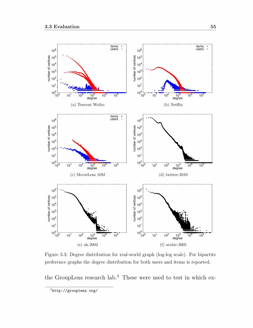
3.3 Evaluation 55
100
101
102
103
104
105
106
100
101
102
103
104
105
num
ber
of vert
ices
degree
itemsusers
(a) Tencent Weibo
100
101
102
103
104
105
106
100
101
102
103
104
105
num
ber
of vert
ices
degree
itemsusers
(b) Netflix
100
101
102
103
104
105
106
100
101
102
103
104
105
num
ber
of vert
ices
degree
itemsusers
(c) MovieLens 10M
100
101
102
103
104
105
106
100
101
102
103
104
105
num
ber
of vert
ices
degree
(d) twitter-2010
100
101
102
103
104
105
106
100
101
102
103
104
105
num
ber
of vert
ices
degree
(e) uk-2002
100
101
102
103
104
105
106
100
101
102
103
104
105
num
ber
of vert
ices
degree
(f) arabic-2005
Figure 3.3: Degree distribution for real-world graph (log-log scale). For bipartite
preference graphs the degree distribution for both users and items is reported.
the GroupLens research lab.4 These were used to test in which ex-
4http://grouplens.org/

56 3. Distributed Matrix Completion
tent the GASGD algorithm benefits from the HDRF partitioning
scheme, both in execution time and convergence speed. We also
selected another 3 graphs from LAW (Laboratory for Web Algorith-
mics) [16, 15]: twitter-2010, uk-2002 and arabic-2005. The latter
were used to test the behavior of HDRF in a more general environ-
ment.
Table 3.2 reports some statistics for these 6 datasets, while figure
3.3 shows their degree distribution.
System Setup. We implemented a stand-alone version of a graph
partitioner that captures the behavior of a DGC framework during
the graph loading and partitioning phase. Within our partitioner,
we implemented the five different algorithms described so far: hash-
ing, DBH, grid, PDS, greedy and HDRF. Furthermore, we compared
HDRF against two offline methods: Ginger [93], an hybrid solu-
tion that tries to combine both edge-cut and vertex-cut approaches
together, and METIS [59], a well-known edge-cut partitioning algo-
rithm. To compute the replication factor delivered by METIS, we
used the same strategy of [47]: every edge-cut forces the two spanned
parts in maintaining a replica of both vertices and a copy of the edge
data. Experiments were run on an Intel Xeon 8-core machine with
32GB of memory running the GNU/Linux 64-bit operating system.
To run realistic tests needed to measure execution time, we imple-
mented and integrated HDRF into GraphLab v2.2. In each test,
we loaded and partitioned the input graph using HDRF or one
of the comparison algorithms. Experiments with GraphLab where

3.3 Evaluation 57
conducted both: (1) on an Amazon EC2 cluster, consisting of 315
m3.large6 Linux instances in the US West (Oregon) region, and (2)
on a cluster consisting of 8 machines with dual 16-core Intel Xeon
CPUs and 128GB of memory each, where we experimented with 32,
64 and 128 parts by running multiple instances on a single machine.
We also evaluated the convergence of GASGD with respect to dif-
ferent input partitioner strategy, using a simulator.7 As parameters,
we used d = 100 latent factors, λ = 0.05 for all variables, a constant
learning rate of η = 0.005, and ran 100 epochs.
Data input order. Since the input dataset is consumed as a stream
of edges, the input order can affect the performance of the parti-
tioning algorithm. We considered three different stream orders as
in [128]: random, where edges arrive according to a random per-
mutation; BFS, where the edge order is generated by selecting a
vertex uniformly at random and performing a breadth first search
visit starting from that vertex; DFS, that works as BFS except for
the visit algorithm that is depth-first search. All reported results
are based on a random input order unless otherwise mentioned in
the text.
3.3.2 Performance Evaluation
The experimental results reported in this section are organized as
follows: we first report on experiments that show the benefits that
5This number of parts fits constraints for PDS.62 vCPU and 7.5 Memory (GB)7The source code is available at https://github.com/fabiopetroni/GASGD.

58 3. Distributed Matrix Completion
1
2
4
8
16
4 8 16 32 64 128 256
replic
ation facto
r
parts
(a) Tencent Weibo
1
2
4
8
16
4 8 16 32 64 128 256
replic
ation facto
r
parts
PDSgrid
hashingDBH
greedyHDRF
(b) Netflix
1
2
4
8
16
4 8 16 32 64 128 256
replic
ation facto
r
parts
PDSgrid
hashingDBH
greedyHDRF
(c) MovieLens 10M
Figure 3.4: Replication factor varying the number of target parts (log-log scale).
HDRF brings to GASGD and, in general, the ability of HDRF to
deliver the best overall performance in terms of execution time with
the smallest overhead (replication factor) and close to optimal load
balance when executed on real-world graphs. We then study how
HDRF performance is affected by changes in the characteristics of
the input dataset and changes in the target number of parts. Fi-
nally, the last set of results analyze the sensitivity of HDRF to input
stream ordering.

3.3 Evaluation 59
1
2
4
8
16
Tencent Weibo Netflix MovieLens 10M
replic
ation facto
r
PDS
7.9
11.3 11.5greedy
2.8
8.1
10.7
DBH
1.5
7.1
12.9HDRF
1.3
4.9
9.1
1
2
4
8
16
Tencent Weibo Netflix MovieLens 10M
replic
ation facto
r
PDS
greedy
DBH
HDRF
(a) Streaming algorithms
1
2
4
8
16
Tencent Weibo Netflix MovieLens 10M
replic
ation facto
r
38.6 40.9METIS
14.8
Ginger
1.4
5.2
10.9
HDRF
1.3
4.9
9.1
(b) Offline algorithms
Figure 3.5: Replication factor (log scale) with |S| = 133. HDRF is compared
against both streaming and offline solutions.
GASGD Runtime
We first measured HDRF performance against other streaming par-
titioning algorithms on our set of real-world bipartite preference
graphs. These experiments were run by partitioning the input graphs
on a set of target parts in the range [3, 256] with our stand-alone par-
titioner. Figure 3.4 reports the replication factor that the consid-
ered partitioning algorithms achieve on the different input graphs.8
Moreover, figure 3.5a provides a snapshot of the evaluation, by set-
ting the number of target parts to 133, a number compliant with
PDS constraints. It can be observed that HDRF is the algorithm
that provides the smallest replication factor for all the considered
datasets.
In particular, for the Weibo dataset it is possible to observe how
HDRF and DBH are the best performers as they both exploit ver-
tex degrees. In all the other datasets HDRF is always the best per-8Due to specific constraints imposed by the PDS and grid algorithms on the total number
of parts, their data points are not aligned with those of the other algorithms.

60 3. Distributed Matrix Completion
former, albeit with larger absolute RF values. Summarizing, on the
considered datasets HDRF achieves on average a replication factor
about 40% smaller than DBH, more than 50% smaller than greedy,
almost 3× smaller than PDS, more than 4× smaller than grid and
almost 14× smaller than hashing.
Next, we compared HDRF against two offline partitioning algo-
rithms: Ginger and METIS. Note that these offline solutions have
full knowledge of the input graph that can be exploited to drive their
partitioning choices. Figure 3.5b compares the replication factor
achieved by these two solutions and HDRF (we maintain |S| = 133
to be coherent with figure 3.5a). The poor performance of METIS
was an expected result since it has been proved that edge-cut ap-
proaches perform worse than vertex-cut ones on power-law graphs
[47]. Moreover, the scope of Metis is to balance vertex load among
parts. However, HDRF outperforms Ginger as well, by reducing
its replication factor by 10% on average. In addition, HDRF has
the clear advantage of consuming the graph in a one-pass fashion
while Ginger needs several passes over the input data to converge.
These results show that HDRF is always able to provide a smaller
average replication factor with respect to all other algorithms, both
streaming and offline.
Figure 3.6 reports the load relative standard deviation produced by
the tested streaming algorithms when run on the MovieLens 10M
dataset with a variable number of target parts (results for other
datasets showed similar behavior so we omit them). The curves show
that HDRF and greedy provide the best performance as the number
of target parts grows. As expected, hashing provides well balanced

3.3 Evaluation 61
0
1
2
3
4
5
6
7
8 16 32 64 128 256lo
ad r
ela
tive s
tandard
devia
tion (
%)
parts
PDSgridgreedyDBHHDRFhashing
Figure 3.6: Load relative standard deviation produced by different partitioning
algorithms on the MovieLens 10M dataset.
parts, but it still performs worse that the other algorithms as its ex-
pected behavior with respect to load balancing is only probabilistic.
Grid performs similarly, even if its more complex constraints induce
some skew in load. DBH and PDS are the worse performers, with
load skew growing at a fast pace as the number of target parts grows.
Note that replication factor reflects communication cost, and edge-
imbalance reflects workload-imbalance; providing good performance
with these two metrics means that HDRF can provide partition-
ing results that make the execution of application algorithms more
efficient.
To this end, we studied how much all of this translates to a per-
formance improvement with respect to the execution time. To in-
vestigate the impact of the different partitioning techniques we ran
the GASGD algorithm on GraphLab. Figure 3.7a shows the result
of experiments that were run on an EC2 cluster with 31 machines.
Figure 3.7b reports the results for the Tencent Weibo, with 32, 64
and 128 parts respectively, using a cluster of eight machines. Both
figures report the measured speed-up, obtained by using HDRF to
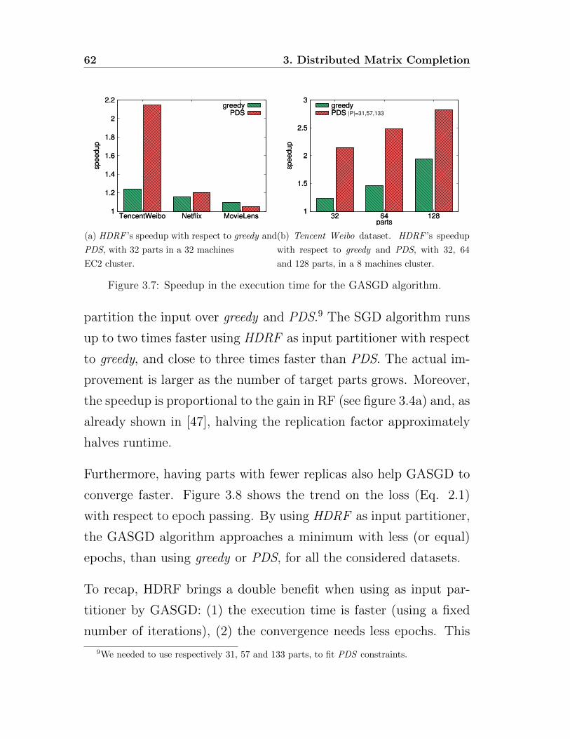
62 3. Distributed Matrix Completion
1
1.2
1.4
1.6
1.8
2
2.2
TencentWeibo Netflix MovieLens
speedup
greedyPDS
1
1.2
1.4
1.6
1.8
2
2.2
TencentWeibo Netflix MovieLens
speedup
greedyPDS
(a) HDRF ’s speedup with respect to greedy and
PDS, with 32 parts in a 32 machines
EC2 cluster.
1
1.5
2
2.5
3
32 64 128
speedup
parts
greedyPDS
1
1.5
2
2.5
3
32 64 128
speedup
parts
greedyPDS |P|=31,57,133
(b) Tencent Weibo dataset. HDRF ’s speedup
with respect to greedy and PDS, with 32, 64
and 128 parts, in a 8 machines cluster.
Figure 3.7: Speedup in the execution time for the GASGD algorithm.
partition the input over greedy and PDS.9 The SGD algorithm runs
up to two times faster using HDRF as input partitioner with respect
to greedy, and close to three times faster than PDS. The actual im-
provement is larger as the number of target parts grows. Moreover,
the speedup is proportional to the gain in RF (see figure 3.4a) and, as
already shown in [47], halving the replication factor approximately
halves runtime.
Furthermore, having parts with fewer replicas also help GASGD to
converge faster. Figure 3.8 shows the trend on the loss (Eq. 2.1)
with respect to epoch passing. By using HDRF as input partitioner,
the GASGD algorithm approaches a minimum with less (or equal)
epochs, than using greedy or PDS, for all the considered datasets.
To recap, HDRF brings a double benefit when using as input par-
titioner by GASGD: (1) the execution time is faster (using a fixed
number of iterations), (2) the convergence needs less epochs. This
9We needed to use respectively 31, 57 and 133 parts, to fit PDS constraints.
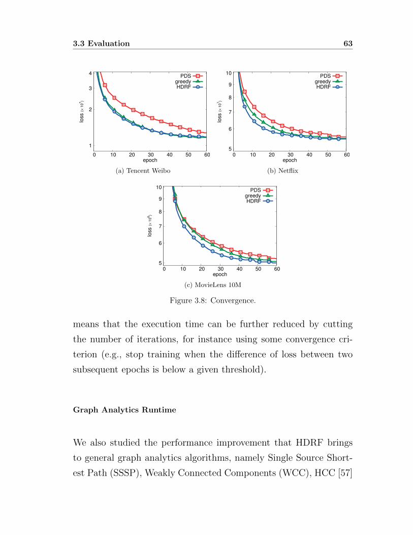
3.3 Evaluation 63
1
2
3
4
0 10 20 30 40 50 60
loss (
× 1
07)
epoch
PDSgreedyHDRF
(a) Tencent Weibo
5
6
7
8
9
10
0 10 20 30 40 50 60
loss (
× 1
07)
epoch
PDSgreedyHDRF
(b) Netflix
5
6
7
8
9
10
0 10 20 30 40 50 60
loss (
× 1
06)
epoch
PDSgreedyHDRF
(c) MovieLens 10M
Figure 3.8: Convergence.
means that the execution time can be further reduced by cutting
the number of iterations, for instance using some convergence cri-
terion (e.g., stop training when the difference of loss between two
subsequent epochs is below a given threshold).
Graph Analytics Runtime
We also studied the performance improvement that HDRF brings
to general graph analytics algorithms, namely Single Source Short-
est Path (SSSP), Weakly Connected Components (WCC), HCC [57]

64 3. Distributed Matrix Completion
algorithm cpu network
SSSP low low
WCC low medium
HCC low medium
PR medium high
GASGD high high
Table 3.3: Algorithms used when measuring execution time with different input
graphs.
and Page Rank (PR). Table 3.3 provides more information on the al-
gorithms in terms of cpu and network resource usage. Here, clearly,
the tested application algorithm plays an important role: some al-
gorithms may concentrate computation on high-degree nodes while
others may place a uniform load on the input graph. In these cases,
we expect different improvements. However, the reduction in syn-
chronization overhead among replicas induced by a smaller average
replication factor shall in any case positively impact performance.
These experiments were run on an EC2 cluster with 31 machines
running GraphLab.
Figure 3.9 reports the replication factor for the twitter-2010, uk-
2002 and arabic-2005 datasets. In all our tests HDRF outperforms
competing solutions.
Figure 3.10 reports the measured speed-up of graph analytics algo-
rithms, obtained by using HDRF to partition the input over greedy
(figure 3.10a) and PDS (figure 3.10b). The results confirmed our
intuitions: the speedup is proportional to both the advantage in
replication factor and the actual network usage of the algorithm.
The speedup it is larger for IO-intensive algorithms (e.g., GASGD
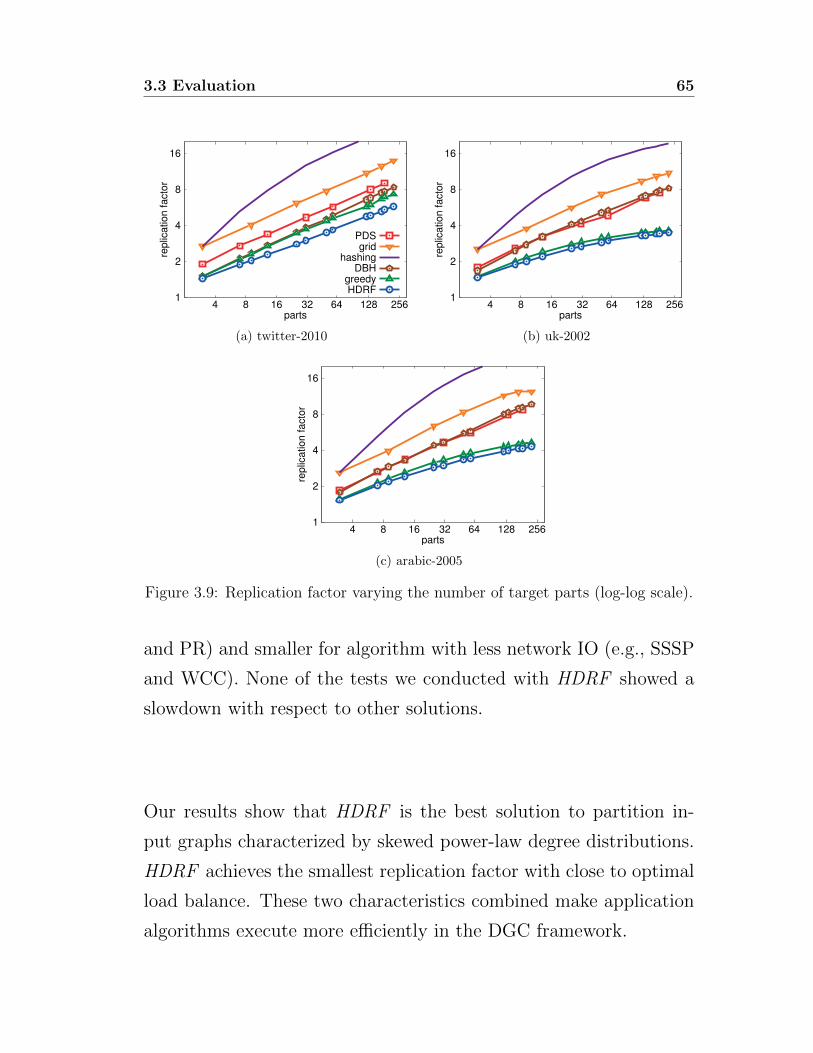
3.3 Evaluation 65
1
2
4
8
16
4 8 16 32 64 128 256
replic
ation facto
r
parts
PDSgrid
hashingDBH
greedyHDRF
(a) twitter-2010
1
2
4
8
16
4 8 16 32 64 128 256
replic
ation facto
r
parts
(b) uk-2002
1
2
4
8
16
4 8 16 32 64 128 256
replic
ation facto
r
parts
(c) arabic-2005
Figure 3.9: Replication factor varying the number of target parts (log-log scale).
and PR) and smaller for algorithm with less network IO (e.g., SSSP
and WCC). None of the tests we conducted with HDRF showed a
slowdown with respect to other solutions.
Our results show that HDRF is the best solution to partition in-
put graphs characterized by skewed power-law degree distributions.
HDRF achieves the smallest replication factor with close to optimal
load balance. These two characteristics combined make application
algorithms execute more efficiently in the DGC framework.
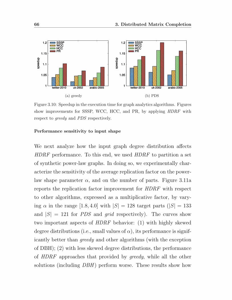
66 3. Distributed Matrix Completion
1
1.05
1.1
1.15
1.2
twitter-2010 uk-2002 arabic-2005
speedup
SSSPWCCHCCPR
1
1.05
1.1
1.15
1.2
twitter-2010 uk-2002 arabic-2005
speedup
SSSPWCCHCCPR
(a) greedy
1
1.05
1.1
1.15
1.2
twitter-2010 uk-2002 arabic-2005
speedup
SSSPWCCHCCPR
1
1.05
1.1
1.15
1.2
twitter-2010 uk-2002 arabic-2005
speedup
SSSPWCCHCCPR
(b) PDS
Figure 3.10: Speedup in the execution time for graph analytics algorithms. Figures
show improvements for SSSP, WCC, HCC, and PR, by applying HDRF with
respect to greedy and PDS respectively.
Performance sensitivity to input shape
We next analyze how the input graph degree distribution affects
HDRF performance. To this end, we used HDRF to partition a set
of synthetic power-law graphs. In doing so, we experimentally char-
acterize the sensitivity of the average replication factor on the power-
law shape parameter α, and on the number of parts. Figure 3.11a
reports the replication factor improvement for HDRF with respect
to other algorithms, expressed as a multiplicative factor, by vary-
ing α in the range [1.8, 4.0] with |S| = 128 target parts (|S| = 133
and |S| = 121 for PDS and grid respectively). The curves show
two important aspects of HDRF behavior: (1) with highly skewed
degree distributions (i.e., small values of α), its performance is signif-
icantly better than greedy and other algorithms (with the exception
of DBH); (2) with less skewed degree distributions, the performance
of HDRF approaches that provided by greedy, while all the other
solutions (including DBH ) perform worse. These results show how
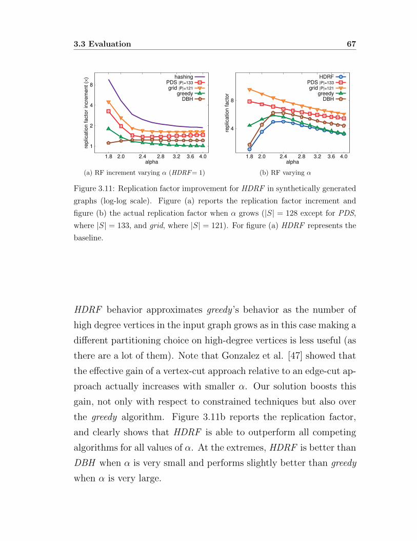
3.3 Evaluation 67
1
2
4
8
1.8 2.0 2.4 2.8 3.2 3.6 4.0
replic
ation facto
r in
cre
ment (×
)
alpha
hashingPDS |P|=133
grid |P|=121
greedyDBH
(a) RF increment varying α (HDRF= 1)
4
8
1.8 2.0 2.4 2.8 3.2 3.6 4.0
replic
ation facto
r
alpha
HDRFPDS |P|=133
grid |P|=121
greedyDBH
(b) RF varying α
Figure 3.11: Replication factor improvement for HDRF in synthetically generated
graphs (log-log scale). Figure (a) reports the replication factor increment and
figure (b) the actual replication factor when α grows (|S| = 128 except for PDS,
where |S| = 133, and grid, where |S| = 121). For figure (a) HDRF represents the
baseline.
HDRF behavior approximates greedy ’s behavior as the number of
high degree vertices in the input graph grows as in this case making a
different partitioning choice on high-degree vertices is less useful (as
there are a lot of them). Note that Gonzalez et al. [47] showed that
the effective gain of a vertex-cut approach relative to an edge-cut ap-
proach actually increases with smaller α. Our solution boosts this
gain, not only with respect to constrained techniques but also over
the greedy algorithm. Figure 3.11b reports the replication factor,
and clearly shows that HDRF is able to outperform all competing
algorithms for all values of α. At the extremes, HDRF is better than
DBH when α is very small and performs slightly better than greedy
when α is very large.

68 3. Distributed Matrix Completion
100
101
100
101
replic
ation facto
r
µ
hashing
PDS
greedyBFSDFS
random
(a) replication factor
|E|
100
101
max p
art
siz
e (
ed
ge
ca
rdin
alit
y)
µ
pds, hashing
greedy
|E||
|S|BFSDFS
random
(b) max edge cardinality
|V|
100
101
max p
art
siz
e (
ve
rte
x c
ard
ina
lity)
µ
hashing
pds
greedy
|V|||S|
BFSDFS
random
(c) max vertex cardinality
Figure 3.12: HDRF behavior on the Netflix dataset varying µ, with input edge
stream either random or ordered (DFS or BFS graph visits). Reference grey lines
represent greedy, hashing and PDS performance.
Performance sensitivity to input order
A shortcoming of the standard greedy algorithm is its inability to
effectively handle streaming of input edges when they are ordered.
If the algorithm receives the edges ordered such that two subsequent
edges always share a vertex, the greedy algorithm always places all
the edges and their adjacent vertices in a single part. This leads to
a degenerate partitioning where, whatever the target parts number
is, only a single part holds the whole input graph with the other

3.3 Evaluation 69
parts being empty. While this eliminates the need for vertex repli-
cas, the final result is clearly far from being desirable as all of the
computation load will be incurred by a single node in the computing
cluster.
To overcome this limitation, we explicitly introduced the parameter
µ in the computation of the score for each part in HDRF (equations
(3.6) and (3.8)), that defines the importance of the load balance in
the edge placement decision (section 3.2.3). Figure 3.12 shows the
result of an experiment run on the Netflix dataset, where the input
stream of edges is ordered according to either a depth-first-search
(DFS) or a breadth-first-search (BFS) visit on the graph. The figure
shows the average replication factor (figure 3.12a), the size of the
largest part expressed as number of contained edges (figure 3.12b)
and the size of the largest part expressed as number of contained
vertices (figure 3.12c) all while varying the value of µ in the range
[0.1, 100] (log-log axes). All three figures report the performance
obtained with the greedy, hashing and PDS algorithms as horizontal
grey lines for reference.
If we first consider the average replication factor (Figure 3.12a), we
can see that as long as µ ≤ 1 HDRF, the CBAL term in HDRF ’s
cost function is always smaller than 1 and thus makes the algorithm
behave exactly as the standard greedy algorithm (curves BFS and
DFS); all edges are placed in a single part and no vertex is replicated.
This behavior is confirmed by the size of the largest part that in this
case contains exactly |E| edges and |V | vertices (Figures 3.12b and
3.12c).
70 3. Distributed Matrix Completion
For µ > 1, even for values only slightly larger than 1, the CBAL fac-
tor starts to play a fundamental role in balancing the load among
the available parts: the average replication factor for HDRF with
both DFS and BFS inputs is just slightly larger than what is achiev-
able with a random input and still substantially lower than what is
achievable with PDS or hashing (figure 3.12a). At the same time,
the size of the largest part drops to its minimum (figures 3.12b and
3.12c) indicating that the algorithm immediately delivers close to
perfect load balancing (i.e., |E|/|S| edges per part). With these
values of µ, the number of vertices hosted in the largest part ap-
proaches its theoretical minimum |V |/|S|; this value is hypothetical
as it is achievable only when the graph is composed of |S| connected
components with the same number of vertices. The difference shown
by HDRF itself when run over a BFS or DFS ordered input with
respect to the randomized input can be traced back to our hypothe-
sis that partial information on vertex degrees collected at runtime is
a good proxy for the actual degree of the vertices; this hypothesis,
in fact, is not true if the input is not randomized: when vertices of
the input graph are visited in a non random order, we cannot expect
the partitioner to see incoming vertices as a completely uniform ran-
dom stream. As a consequence, the partial information on vertex
degrees can be wrong and drive HDRF toward inefficient placement
decisions.
By increasing µ toward larger values, the effect of CBAL dominates
the HDRF cost function; instead of selecting vertices to be replicated
on the basis of their degree, the algorithm tries to simply balance
parts sizes. In this case, its behavior quickly approaches the behavior
3.4 Summary 71
typical of the hashing algorithm: large average replication factor,
with close to perfect load balancing and the largest part containing
a number of vertices that approaches |V |.
These results show that (1) the CBAL term in HDRF score computa-
tion plays an effective role in providing close-to-perfect load balanc-
ing among parts while keeping a low average replication factor, and
(2) by setting the value of µ slightly larger than 1, it is possible to
let HDRF work at a “sweet spot” where it can deliver the best per-
formance, even when working on an ordered stream of edges. This
last point makes HDRF particularly suitable for application settings
where it is not possible to randomize the input stream before feeding
it to the graph partitioning algorithm.
3.4 Summary
Distributed matrix completion algorithms are designed for large
scale instances of the problem. Remarkable examples are stratified
SGD and asynchronous SGD. For these algorithms, system perfor-
mance is often determined by the input partitioning strategy, which
impacts the communication cost and the workload balance among
compute resources. We proposed a transition to a to a graph-based
data representation model. This allows to use graph partitioning
algorithm to tackle the above challenges.
We proposed HDRF, a novel stream-based graph partitioning algo-
rithm. HDRF is based on a greedy vertex-cut approach that lever-
ages information on vertex degrees. Through a theoretical analysis

72 3. Distributed Matrix Completion
and an extensive experimental evaluation on real-world as well as
synthetic graphs using both a stand-alone partitioner and implemen-
tation of HDRF in GraphLab, we showed that HDRF is overall the
best performing partitioning algorithm for graphs characterized by
power-law degree distributions, that is HDRF provides the smallest
average replication factor with close to optimal load balance. These
two characteristics put together allow HDRF to significantly reduce
the time needed to perform computation on graphs and makes it the
best choice for partitioning graph data. In particular, distributed
matrix completion algorithms execute and converge faster when us-
ing HDRF as input partitioner.

CHAPTER 4
Context-Aware Matrix Completion
Computers are useless. They can only give you answers.
Pablo Picasso
The context in which relationships are observed is an important
source of information, whose exploitation can help in the task of
understanding and modeling them, therefore to the ultimate goal of
providing better predictions. For example, leveraging the purpose
of a travel, a hotel recommender system would provide more accu-
rate accommodation suggestions, targeted to, for instance, business
trips rather than holidays. However, incorporating generic contex-
tual information inside a latent factor model is challenging. In the
following, we review some of the current context-aware matrix com-
pletion techniques, developed mostly to enhance the performance of
recommender systems.
74 4. Context-Aware Matrix Completion
4.1 Context-Aware Algorithms
There is a large body of research that aims at extending matrix
completion models to include such contextual information, mainly
focused on collaborative filtering in recommender systems (see [2,
96, 114] for excellent surveys on this topic). Most of the proposed
solutions are customized algorithms that integrate a specific infor-
mation, such as timestamps [65], user tags [134], geolocations [135],
but fail in capturing generic contextual data.,
A remarkable example of a general framework are collective matrix
factorization (or joint matrix factorization) models [116, 72], which
simultaneously factorize the user-item rating matrix and other ma-
trices containing attributes of both users (e.g., user’s gender, age,
and hobbies) and items (e.g., category and content). However, such
models are unable to consider the information associated with the
interaction between user and item, e.g., the rating event.
One way to integrate interaction-associated contextual information
is using tensor completion models [61, 58, 101, 82, 112]. Such al-
gorithms add a dimension to the user-item rating matrix with con-
textual data, creating a tensor, that can be factorized using existing
techniques, as, for instance, Candecomp/Parafac [61] or Tucker [58]
decompositions. Tensor completion models, however, suffer from
limited scalability with respect to the amount of contextual infor-
mation considered. The computational complexity of such models is,
in fact, exponential with the number of contextual variables included
in the model, and this hampers their applicability in real-world sce-
narios.
4.1 Context-Aware Algorithms 75
Factorization machines [100, 97, 98] are currently considered the
best solutions for context-aware matrix completion, due to their ad-
vantages with respect to both scalability and accuracy. In fact, they
solve the scalability issues of tensor completion models, experiencing
a linear time complexity in the number of contextual variables con-
sidered. Factorization machines associate a latent factor vector with
each contextual variable. The innovative idea is to model all itera-
tion between pairs of variables (e.g., users, items and context) with
the target (e.g., the rating) using factorized interaction parameters.
Such parameters are obtained computing the dot product between
the latent factor vectors associated with the two variables in the pair
(see below for further details).
All existing solutions for context-aware matrix completion require
in input both positive and negative evidence, that is the revealed
entries in the data matrix have multiple values, a situation that
correspond to the presence of explicit feedback in recommender sys-
tems and that can be managed using the regularized squared loss
optimization criterion.
In what follows we will show how to integrate contextual informa-
tion inside a matrix completion model in those cases in which only
positive evidence exist in input, that is the revealed entries in the
matrix have all the same value, a situation that correspond to the
presence of implicit feedback in recommender systems and that can
be managed using the Bayesian personalized ranking optimization
criterion. To this end, we use, as baseline application scenario, a
popular natural language processing task: open relation extraction.
76 4. Context-Aware Matrix Completion
4.2 Open Relation Extraction
New generation algorithms for web information retrieval (IR) make
use of a knowledge base (KB) to increase their accuracy. A clear
example of this is the Google knowledge graph [117]. The basic idea
of these techniques is to match the words in a query to real world
entities (e.g., a person, a location, etc.) and use real world connec-
tions among these entities to improve the task of providing the user
with the proper content s/he was looking for. One popular way to
represent such KB is through a graph structure, where entities are
connected to each other through relations (ex, ”born in”, ”contained
by”). This is the idea, for instance, of the web’s linked open data
cloud [28, 8, 9], a public accessible KB consisting of over 60 billion
known facts. Such structures provide exciting opportunities, not
only for IR but also for the entire scientific community. However,
despite their size, these KBs are still far from being completed. For
instance 75% of the people in Freebase [17] have unknown nation-
ality, the place of birth attribute is missing for 71% of all people
[130], and coverage for less common relations is even lower. More-
over, relational data can not only be incomplete but also uncertain,
noisy and include false information. Automatic methods for relation
extraction are therefore needed in order to fill missing information
and remove incorrect facts. These algorithms should not only use
the information already present in the KB but also scan the web,
extracting new information from natural language text in web pages.
Open relation extraction (open RE) is the task of extracting new
facts for a potentially unbounded set of relations from various sources
4.2 Open Relation Extraction 77
such as knowledge bases or natural language text. The task is closely
related to targeted information extraction (IE) [80, 122, 78], which
aims to populate a knowledge base (KB) with new facts for the KB’s
relations, such as wasBornIn(Sepp Herberger, Mannheim). However,
targeted IE methods are inherently limited to an (often small) set of
predefined relations, i.e., they are not “open”. The open RE task is
also related to open information extraction (open IE) [11, 40, 32],
which extracts large amounts of surface relations and their argu-
ments from natural language text. In contrast to targeted IE, the
goal of open IE is to extract all (or most) relations expressed in
natural-language text, whether or not these relations are defined in
a KB. The facts obtained by open IE methods are often not dis-
ambiguated, i.e., the entities and/or the relation are not linked to
a knowledge base; e.g., “criticizes”(“Dante”, “Catholic Church”).1
Although open IE is a domain-independent approach, the extracted
surface relations are purely syntactic and often ambiguous or noisy.
Moreover, open IE methods usually do not “predict” facts that have
not been explicitly observed in the input data. Open RE combines
the above tasks by predicting new facts for an open set of relations.
The key challenge in open RE is to reason jointly over the universal
schema consisting of KB relations and surface relations [104].
4.2.1 Relation Extraction Algorithms
Figure 4.1 presents a taxonomy of existing relation extraction algo-
rithms. The main distinction is between closed and open techniques.
1We mark (non-disambiguated) mentions of entities and relations in quotation marks.
78 4. Context-Aware Matrix Completion
Closed relation extraction solutions aim at predicting new facts for
a set of predefined relations, usually taken from a KB. Existing
methods either reason within the KB itself [43, 85, 36] or lever-
age large text corpora to learn patterns that are indicative of KB
relations [80, 122, 78].
The latter solutions typically make use of distant supervision, i.e.,
they start with a set of seed instances (pairs of entities) for the
relations of interest, search for these seed instances in text, learn a
relation extractor from the so-obtained training data, and optionally
iterate [80, 122, 78].
The former techniques are typically based on tensor completion mod-
els, which use the available data to learn latent semantic representa-
tions of entities (i.e., subjects and objects) and relations in a domain-
independent way; the latent representations are subsequently used to
predict new facts. Tensor completion models conceptually model the
input data as a subject×relation×object tensor, in which non-zero
values correspond to input facts. The tensor is factored to construct
a new tensor in which predicted facts take large non-zero values.
Examples of such tensor factorization models are TripleRank [43],
RESCAL [85, 86], or PITF [36]. Tensor factorization models are
generally well-suited to reason within a KB because they are able to
predict relations between arbitrary pairs of subjects and objects.
Open relation extraction algorithms aim at predicting new facts for
an unbounded set of relations, that came from various sources, such
that natural language text or knowledge bases. Tensor factorization
model are not well-suited for open RE, since these methods suffer
from limited scalability with the number of relations as well as from

4.2 Open Relation Extraction 79
distant supervision
relation extraction
tensor completion
matrix completion
RESCAL PITF NFE CORE
relation clustering
set of predefined relations
"black and white" approach
limited scalability with the number of relations; large prediction space
latent factors models
openclosein-KB in-KB
out of-KB
restricted prediction space(Nickel et al., 2011) (Drumond et al., 2012) (Petroni et al., 2015)(Riedel et al., 2013)
Figure 4.1: Taxonomy of relation extraction algorithms.
their large prediction space [22]. In fact, open RE models are more
general then targeted IE methods in that they additionally reason
about surface relations that do not correspond to KB relations. For
this reason, [104] argued and experimentally validated that open RE
models can outperform targeted IE methods.
One way to jointly reason about KB and surface relations is to clus-
ter the relations : whenever two relations appear in the same cluster,
they are treated as synonymous [50, 115, 132, 124, 79, 4, 30]. For ex-
ample, if “criticizes” and “hates” are clustered together, then we may
predict “hates”(“Dante”, “Catholic Church”) from the fact “crit-
80 4. Context-Aware Matrix Completion
icizes”(“Dante”, “Catholic Church”) (which is actually not true).
The general problem with relation clustering is its “black and white”
approach to relations: either two relations are the same or they are
different. This assumption generally does not hold for the surface re-
lations extracted by open IE systems [104]; examples of other types
of relationships between relations include implication or mutual ex-
clusion.
Matrix completion approaches try to address the above problem: in-
stead of clustering relations, they directly predict facts, by learning
and making use of semantic representations of relations and their
arguments. The semantic representations ideally captures all the
information present in the data; it does not, however, establish a di-
rect relationship (such as synonymy) between different KB or surface
relations. The key difference between matrix and tensor completion
models is that the former restrict the prediction space, i.e., these
models generally cannot predict arbitrary facts. Similar to distant
supervision approaches, matrix completion models focus on predict-
ing facts for which some direct evidence exists. In more detail, most
methods restrict the prediction space to the set of facts for which the
subject and the object share at least some relation in the input data.
For this reason, matrix completion models are not suited for in-KB
reasoning; an individual pair of entities usually does not occur in
more than one KB relation. In the open RE context, however, input
relations are semantically related so that many subject-object pairs
belong to multiple relations. The key advantage of matrix methods
is (1) that this restriction allows them to use additional features—
such as features for each subject-object pair—and (2) that they scale

4.3 Context-Aware Open Relation Extraction 81
(Caesar,Rome)
(Fermi,Rome)
(Fermi,Sapienza)
(de Blasio,NY)
1
1
1
1
1
KB relationsurface relation
employee born in professor at mayor of
tuples x relations
?
? ??
? ??
?
? ? ?
Figure 4.2: Example for representing open RE as a matrix completion problem.
much better with the number of relations. Examples of such matrix
factorization models include [126, 55, 104, 41, 53].
Figure 4.2 shows an example for representing open RE as a matrix
completion problem. The ones correspond to observed fact, either
inside or outside the KB (i.e., containing a surface relation), for
instance employee(Fermi,Sapienza) (in-KB) or “mayor of”(de Bla-
sio,NY) (out of-KB). By completing the matrix is possible to esti-
mate the likelihood of missing facts, for instance, in the example, of
the fact “mayor of”(Caesar,Rome) or “born in”(de Blasio,NY).
4.3 Context-Aware Open Relation Extraction
CORE [90] is a novel matrix completion model that leverages generic
contextual information for open relation extraction. CORE inte-
grates facts from various sources, such as knowledge bases or open

82 4. Context-Aware Matrix Completion
information extractors, as well as the context (e.g., metadata about
extraction sources, lexical context, or type information) in which
these facts have been observed.
Consider for example the sentence “Tom Peloso joined Modest Mouse
to record their fifth studio album”. Open IE systems may extract
the surface fact “join”(TP, MM) from this sentence. Note that sur-
face relation “join” is unspecific; in this case, it refers to becoming
a member of a music band (as opposed to, say, an employee of a
company). Most existing open RE systems use the extracted sur-
face fact for further reasoning, but they ignore the context from
which the fact was extracted. Actually, exploiting contextual in-
formation might be beneficial for open RE. For our example, we
may use standard natural language processing tools like a named
entity recognizer to detect that TP is a person and MM an organi-
zation. These coarse-grained types give us hints about the domain
and range of the “join” relation for the surface fact, although the
actual meaning of “join” still remains opaque. Now imagine that the
above sentence was extracted from a newspaper article published in
the music section. This information can help to infer that “join” in-
deed refers to joining a band. Other contextual information, such as
the words “record” and “album” that occur in the sentence, further
strengthen this interpretation. A context-aware open RE system
should leverage such information to accurately predict facts like “is
band member of”(TP, MM) and “plays with”(TP, MM).
Note that the prediction of the fact “is band member of”(TP, MM) is
facilitated if we make use of a KB that knows that TP is a musician
and MM is a music band. If TP and/or MM are not present in

4.3 Context-Aware Open Relation Extraction 83
the knowledge base, however, such a reasoning does not apply. In
our work, we consider both linked entities (in-KB) and non-linked
entity mentions (out of-KB). Since KB are often incomplete, this
open approach to handle named entities allows us to extract facts
for all entities, even if they do not appear in the KB.
4.3.1 The CORE Model
Input data. We model the input data as a set of observations of
the form (r, t, c), where r refer to a KB or surface relation, t re-
fer to a subject-object pair of entities (or entity mentions) and c to
contextual information. An observation obtained from the above ex-
ample may be (“join”, (TP, MM), { types:(person,org), topic:music,
word:record, word:album, . . . }). Denote by R the set of all observed
relations, by E the set of all observed entities, and by T ⊆ E × Ethe set of all observed entity pairs, which we refer to as tuples. A
fact takes form r(t) and is composed of a relation r ∈ R and a tuple
t ∈ T ; e.g., “join”(TP, MM). Note that there may be multiple ob-
servations for a fact. Finally, denote by C the set of all contextual
variables ; each observation is associated with a set c ⊆ C of context
variables.
Problem definition. The open RE task is to produce a ranked list
of tuples Tr ⊆ T for each relation r ∈ R; the list is restricted to new
tuples, i.e., tuples t ∈ T for which r(t) has not been observed in the
input. The rank of each tuple reflects the model’s prediction of the
likelihood that the corresponding fact is indeed true. A good model
thus ranks correct facts higher than incorrect ones.

84 4. Context-Aware Matrix Completion
Symbol Description
R Relations set
T Tuples set
E Entities set
C Contextual variables set
Tr Ranked list of tuples for relation r
V Variables set; R ∪ T ∪ E ∪ C; Columns set
X Training points; Rows set
d Dimensionality of the completion; rank of the factorization
Table 4.1: Notation for matrix completion algorithms in open relation extraction.
Modeling facts. Denote by V = R ∪ T ∪ E ∪ C the set of all ob-
served relations, tuples, entities, and contextual variables. For ease
of exposition, we refer to the elements of V as variables. We model
the input data in terms of a matrix in which each row corresponds
to a fact (i.e., not an observation) and each column to a variable.
We group columns according to the type of the variables; e.g, there
are relation columns, tuple columns, entity columns, and a group
of columns for each type of contextual information. The matrix is
populated such that in each row the values of each column group
sum up to unity, i.e., we normalize values within column groups.
In particular, we set to 1 the values of the variable of the relation
and the tuple of the corresponding fact. We set to 0.5 the variables
corresponding to the two entities referred to by the fact.
An example is shown in Fig. 4.3. Here the first row, for instance,
corresponds to the fact “born in”(Caesar, Rome). Note that we
model tuples and entities separately: the entity variables expose
which arguments belong to the fact, the tuple variables expose their
order.
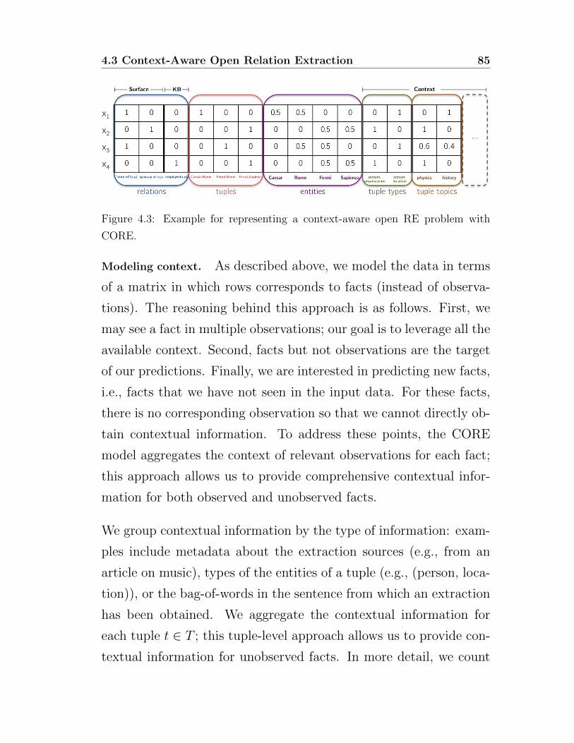
4.3 Context-Aware Open Relation Extraction 85
Figure 4.3: Example for representing a context-aware open RE problem with
CORE.
Modeling context. As described above, we model the data in terms
of a matrix in which rows corresponds to facts (instead of observa-
tions). The reasoning behind this approach is as follows. First, we
may see a fact in multiple observations; our goal is to leverage all the
available context. Second, facts but not observations are the target
of our predictions. Finally, we are interested in predicting new facts,
i.e., facts that we have not seen in the input data. For these facts,
there is no corresponding observation so that we cannot directly ob-
tain contextual information. To address these points, the CORE
model aggregates the context of relevant observations for each fact;
this approach allows us to provide comprehensive contextual infor-
mation for both observed and unobserved facts.
We group contextual information by the type of information: exam-
ples include metadata about the extraction sources (e.g., from an
article on music), types of the entities of a tuple (e.g., (person, loca-
tion)), or the bag-of-words in the sentence from which an extraction
has been obtained. We aggregate the contextual information for
each tuple t ∈ T ; this tuple-level approach allows us to provide con-
textual information for unobserved facts. In more detail, we count
86 4. Context-Aware Matrix Completion
in how many observations each contextual variable has been associ-
ated with the tuple, and then normalize the count values to 1 within
each group of columns. The so-obtained values can be interpreted
as the relative frequencies with which each contextual variable is as-
sociated with the tuple. The contextual information associated with
each fact is given by the aggregated, normalized context of its tuple.
Fig. 4.3 shows context information arranged in two groups: tuple
types and tuple topics. We capture information such as that the
tuple (Caesar, Rome) has only been seen in articles on history or
that tuple (Fermi, Rome) is mentioned in both physics and history
articles (slightly more often in the former). Since context is associ-
ated with tuples, facts 2 and 4 on (Fermi, Sapienza) share contextual
information. This form of context sharing (as well as entity shar-
ing) allows us to propagate information about tuples across various
relations.
Factorization model. CORE employs a matrix completion model
based on factorization machines and the open-world assumption to
capture latent semantic information about the individual variables.
In particular, we associate with each variable v ∈ V a bias term bv ∈R and a latent feature vector f v ∈ Rd, where the dimensionality d of
the latent feature space is a hyperparameter of the model. Denote by
X the set of rows in the input matrix, which we henceforth refer to
as training points. For each training point x ∈ X, denote by xv the
value of variable v ∈ V in the corresponding row of the matrix. Our
model associates with training point x ∈ X a score s(x) computed

4.3 Context-Aware Open Relation Extraction 87
as follows:
s(x) =∑v∈V
xvbv +∑v1∈V
∑v2∈V \{v1}
xv1xv2fTv1f v2 (4.1)
Here the bias terms model the contribution of each individual vari-
able to the final score, whereas the latent feature vectors model the
contribution of all pairwise interactions between variables. Note that
only bias terms and feature vectors corresponding to non-zero en-
tries in x affect the score and that x is often sparse. Since we can
compute s(x) in time linear to both the number of nonzero entries
in x and the dimensionality d [97], score computation is fast. As dis-
cussed below, we (roughly) estimate bias terms and feature vectors
such that observed facts achieve high scores. We may thus think of
each feature vector as a low-dimensional representation of the global
information contained in the corresponding variable.
Prediction. Given estimates for bias terms and latent feature vec-
tors, we rank unobserved facts as follows. Fix a relation r ∈ R and
a tuple t ∈ T such that r(t) has not been observed. As indicated
above, the CORE model overcomes the key problem that there is
no observation, and thus no context, for r(t) by context aggregation
and sharing. In particular, we create an test point x for tuple r(t) in
a way similar to creating data points, i.e., we set the relation, tuple,
and entity variables accordingly and add the aggregated, normal-
ized context of t. Once test point x has been created, we can predict
its score s(x) using Eq. (4.1). We then rank each unobserved tuple
by its so-obtained score, i.e., tuples with higher scores are ranked

88 4. Context-Aware Matrix Completion
higher. The resulting ranking constitutes the list Tr of predicted
facts for relation r.
Bayesian personalized ranking. The parameters of the CORE model
are given by Θ = { bv,f v | v ∈ V }. In approaches based on the
closed-world assumption, Θ is estimated by minimizing the error
between model predictions and target values (e.g., 1 for true facts,
0 for false facts). In our setting of open RE, all our observations
are positive, i.e., we do not have negative training data. One way
to handle the absence of negative training data is to associate a
target value of 0 to all unobserved facts. This closed-world approach
essentially assumes that all unobserved facts are false, which may not
be a suitable assumption for the sparsely observed relations of open
RE. Following [104], we adopt the open-world assumption instead,
i.e., we treat each unobserved facts as unknown. Since factorization
machines originally require explicit target values (e.g., feedback in
recommender systems), we need to adapt parameter estimation to
the open-world setting.
In more detail, we employ a variant of the Bayesian personalized
ranking (BPR) optimization criterion [99]. We associate with each
training point x a set of negative samples X−x . Each negative sample
x− ∈ X−x is an unobserved fact with its associated context (con-
structed as described in the prediction section above). Generally,
the negative samples x− should be chosen such that they are “less
likely” to be true than fact x. We maximize the following optimiza-

4.3 Context-Aware Open Relation Extraction 89
tion criterion:
1
|X|∑x∈X
∑x−∈X−
x
lnσ(δ(x, x−))
|X−x |− λ‖Θx‖2
(4.2)
where σ(x) = 11+e−x denotes the logistic function, δ(x, x−) = s(x)−
s(x−) denotes the difference of scores, and Θx = { bv,f v | xv 6= 0 }the subset of the model parameters relevant for training point x.
Here we use L2 regularization controlled by a single hyperparameter
λ. In essence, the BPR criterion aims to maximize the average
“difference” ln σ(δ(x, x−)) between the score of fact x and each of
its negative samples x−, averaged over all facts. In other words, we
aim to score x higher than each x−. (Note that under the closed-
world assumption, we would instead consider x− as being false.) For
a more in-depth discussion of BPR, see [99].
Sampling negative evidence. To make BPR effective, the set of neg-
ative samples needs to be chosen carefully. A naive approach is to
take the set of all unobserved facts between each relation r ∈ R and
each tuple t ∈ T (or E × E) as the set X−x . The reasoning is that,
after all, we expect “random” unobserved facts to be less likely to be
true than observed facts. This naive approach is problematic, how-
ever, because the set of negative samples is independent of x and
thus not sufficiently informative (i.e., it contains many irrelevant
samples).
To overcome this problem, the negative sample set needs to be re-
lated to x in some way. Since we ultimately use the model to rank

90 4. Context-Aware Matrix Completion
tuples for each relation individually, we consider as negative evi-
dence for x only unobserved facts from the same relation [104]. In
more detail, we (conceptually) build a negative sample set X−r for
each relation r ∈ R. We include into X−r all facts r(t)—again, along
with their context—such that t ∈ T is an observed tuple but r(t)
is an unobserved fact. Thus the subject-object pair t of entities is
not observed with relation r in the input data (but with some other
relation). The set of negative samples associated with each training
point x is defined by the relation r of the fact contained in x, that
is X−x = X−r . Note that we do not actually construct the negative
sample sets; see below.
Parameter estimation. We maximize Eq. (4.2) using stochastic gra-
dient ascent. This allows us to avoid constructing the sets X−x , which
are often infeasibly large, and worked well in our experiments. In
particular, in each stochastic gradient step, we randomly sample a
training point x ∈ X, and subsequently randomly sample a negative
sample x− ∈ X−x . This sampling procedure can be implemented very
efficiently. We then perform the following ascent step with learning
rate η:
Θ← Θ + η∇Θ
(lnσ(δ(x, x−))− λ‖Θx‖2
)One can show that the stochastic gradient used in the formula above
is an unbiased estimate of the gradient of Eq. (4.2). To speed up
parameter estimation, we use a parallel lock-free version of stochastic
gradient ascent as in [95]. This allows the CORE model to handle
(reasonably) large datasets.

4.4 Evaluation 91
size info
facts 453.9k
14.7k Freebase,
174.1k surface linked,
184.5k surface partially-linked,
80.6k surface non-linked.
relations 4.7k94 Freebase,
4.6k surface.
tuples 178.5k
69.5k linked,
71.5k partially-linked,
37.5k non-linked.
entities 114.2k36.8k linked,
77.4k non-linked.
Table 4.2: Dataset statistics.
4.4 Evaluation
We conducted an experimental study on real-world data to com-
pare the CORE model with other state-of-the-art approaches.2 Our
experimental study closely follows the one of [104].
4.4.1 Experimental Setup
Dataset. We made use of the dataset of [104], but extended it with
contextual information. The dataset consisted of 2.5M surface facts
extracted from the New York Times corpus [107], as well as 16k
facts from Freebase [17]. Surface facts have been obtained by using
a named-entity recognizer, which additionally labeled each named
entity mention with its coarse-grained type (i.e., person, organiza-
tion, location, miscellaneous). For each pair of entities found within
2Source code, datasets, and supporting material are available at https://github.com/
fabiopetroni/CORE
92 4. Context-Aware Matrix Completion
a sentence, the shortest dependency path between these pairs was
taken as surface relation. The entity mentions in each surface fact
were linked to Freebase using a simple string matching method. If
no match was found, the entity mention was kept as is. There were
around 2.2M tuples (distinct entity pairs) in this dataset, out of
which 580k were fully linked to Freebase. For each of these tuples,
the dataset additionally included all of the corresponding facts from
Freebase. Using the metadata3 of each New York Times article, we
enriched each surface fact by the following contextual information:
news desk (e.g., sports desk, foreign desk), descriptors (e.g., finances,
elections), online section (e.g., sports, business), section (e.g., a, d),
publication year, and bag-of-words of the sentence from which the
surface fact has been extracted.
Training data. From the raw dataset described above, we filtered out
all surface relations with less than 10 instances, and all tuples with
less than two instances, as in [104]. Tab. 4.2 summarizes statistics
of the resulting dataset. Here we considered a fact or tuple as linked
if both of its entities were linked to Freebase, as partially-linked if
only one of its entities was linked, and as non-linked otherwise. In
contrast to previous work [104, 22], we retain partially-linked and
non-linked facts in our dataset.
Evaluation set. Open RE models produce predictions for all rela-
tions and all tuples. To keep the experimental study feasible and
comparable to previous studies, we use the full training data but
evaluate each model’s predictions on only the subsample of 10k tu-
ples (≈ 6% of all tuples) of [104]. The subsample consisted of 20%
3Further information can be found at htps://catalog.ldc.upenn.edu/LDC2008T19.
4.4 Evaluation 93
linked, 40% partially-linked and 40% non-linked tuples. For each
(surface) relation and method, we predicted the top-100 new facts
(not in training) for the tuples in the subsample.
Considered methods. We compared various forms of the CORE model
with PITF and the matrix factorization model NFE. Our study fo-
cused on these two factorization models because they outperformed
other models (including non-factorization models) in previous stud-
ies [104, 22]. All models were trained with the full training data
described above.
PITF [36]. PITF is a recent tensor factorization method designed
for within-KB reasoning. PITF is based on factorization machines
so that we used our scalable CORE implementation for training the
model.
NFE [104]. NFE is the full model proposed in the “universal schema”
work of [104]. It uses a linear combination of three component mod-
els: a neighborhood model (N), a matrix factorization model (F),
and an entity model (E). The F and E models together are similar
(but not equal) to the CORE model without context. The NFE
model outperformed tensor models [22] as well as clustering meth-
ods and distantly supervised methods in the experimental study of
[104] for open RE tasks. We use the original source code of [104] for
training.
CORE. We include multiple variants of the model in the experi-
mental study, each differing by the amount of context being used.
We consider as context the article metadata (m), the tuple types (t)
94 4. Context-Aware Matrix Completion
and the bag-of-words (w). Each tuple type is a pair of subject-object
types of (e.g. (person, location)). The basic CORE model uses rela-
tions, tuples and entities as variables. We additionally consider the
CORE+t, CORE+w, CORE+mt, and CORE+mtw models, where
the suffix indicates which contextual information has been included.
The total number of variables in the resulting models varied be-
tween 300k (CORE) to 350k (CORE+mtw). We used a modified
version of libfm for training.4 Our version adds support for BPR
and parallelizes the training algorithm.
Methodology. To evaluate the prediction performance of each
method, we followed [104]. We considered a collection of 19 Freebase
relations (Tab. 4.3) and 10 surface relations (Tab. 4.4) and restrict
predictions to tuples in the evaluation set.
Evaluation metrics. For each relation and method, we computed the
top-100 evaluation set predictions and labeled them manually. We
used as evaluation metrics the mean average precision defined as:
MAP100# =
∑100k=1 Ik · P@k
min{100,#}(4.3)
where indicator Ik takes value 1 if the k-th prediction is true and
0 otherwise, and # denotes the number of true tuples for the rela-
tion in the top-100 predictions of all models. The denominator is
included to account for the fact that the evaluation set may include
less than 100 true facts. MAP100# reflects how many true facts are
found by each method as well as their ranking. If all # facts are
found and ranked top, then MAP100# = 1. Note that this definition
4the surce code is available at https://github.com/fabiopetroni/libfm

4.4 Evaluation 95
of MAP100# differs slightly from [104]; this metric is more robust be-
cause it is based on completely labeled evaluation data. To compare
the prediction performance of each system across multiple relations,
we averaged MAP100# values, in both an unweighted and a weighted
(by #) fashion.
Parameters. For all systems, we used d = 100 latent factors, λ =
0.01 for all variables, a constant learning rate of η = 0.05, and ran
1000 epochs of stochastic gradient ascent. These choices correspond
to the ones of [104]; no further tuning was performed.
4.4.2 Results
Prediction performance. The results of our experimental study are
summarized in table 4.3 (Freebase relations) and table 4.4 (surface
relations). As mentioned before, all reported numbers are with re-
spect to our evaluation set. Each entry shows the number of true
facts in the top-100 predictions and, in parentheses, the MAP100#
value. The # column list the total number of true facts found by at
least one method. The last two lines show the aggregated MAP100#
scores.
We start our discussion with the results for Freebase relations (ta-
ble 4.3 and figure 4.4). First note that the PITF model generally
did not perform well; as discussed before, tensor factorization mod-
els such as PITF suffer from a large prediction space and cannot
incorporate tuple-level information. NFE and CORE, both matrix
factorization models, performed better and were on par with each
other. This indicates that the use of factorization machines does not
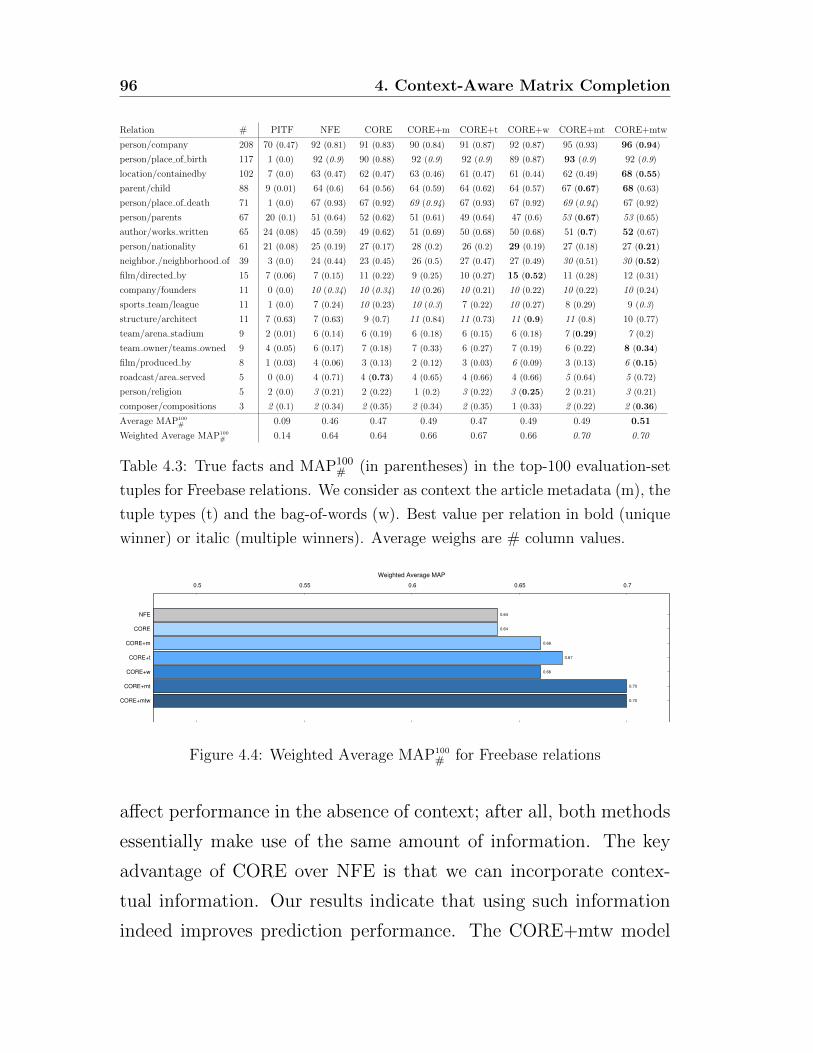
96 4. Context-Aware Matrix Completion
Relation # PITF NFE CORE CORE+m CORE+t CORE+w CORE+mt CORE+mtw
person/company 208 70 (0.47) 92 (0.81) 91 (0.83) 90 (0.84) 91 (0.87) 92 (0.87) 95 (0.93) 96 (0.94)
person/place of birth 117 1 (0.0) 92 (0.9) 90 (0.88) 92 (0.9) 92 (0.9) 89 (0.87) 93 (0.9) 92 (0.9)
location/containedby 102 7 (0.0) 63 (0.47) 62 (0.47) 63 (0.46) 61 (0.47) 61 (0.44) 62 (0.49) 68 (0.55)
parent/child 88 9 (0.01) 64 (0.6) 64 (0.56) 64 (0.59) 64 (0.62) 64 (0.57) 67 (0.67) 68 (0.63)
person/place of death 71 1 (0.0) 67 (0.93) 67 (0.92) 69 (0.94) 67 (0.93) 67 (0.92) 69 (0.94) 67 (0.92)
person/parents 67 20 (0.1) 51 (0.64) 52 (0.62) 51 (0.61) 49 (0.64) 47 (0.6) 53 (0.67) 53 (0.65)
author/works written 65 24 (0.08) 45 (0.59) 49 (0.62) 51 (0.69) 50 (0.68) 50 (0.68) 51 (0.7) 52 (0.67)
person/nationality 61 21 (0.08) 25 (0.19) 27 (0.17) 28 (0.2) 26 (0.2) 29 (0.19) 27 (0.18) 27 (0.21)
neighbor./neighborhood of 39 3 (0.0) 24 (0.44) 23 (0.45) 26 (0.5) 27 (0.47) 27 (0.49) 30 (0.51) 30 (0.52)
film/directed by 15 7 (0.06) 7 (0.15) 11 (0.22) 9 (0.25) 10 (0.27) 15 (0.52) 11 (0.28) 12 (0.31)
company/founders 11 0 (0.0) 10 (0.34) 10 (0.34) 10 (0.26) 10 (0.21) 10 (0.22) 10 (0.22) 10 (0.24)
sports team/league 11 1 (0.0) 7 (0.24) 10 (0.23) 10 (0.3) 7 (0.22) 10 (0.27) 8 (0.29) 9 (0.3)
structure/architect 11 7 (0.63) 7 (0.63) 9 (0.7) 11 (0.84) 11 (0.73) 11 (0.9) 11 (0.8) 10 (0.77)
team/arena stadium 9 2 (0.01) 6 (0.14) 6 (0.19) 6 (0.18) 6 (0.15) 6 (0.18) 7 (0.29) 7 (0.2)
team owner/teams owned 9 4 (0.05) 6 (0.17) 7 (0.18) 7 (0.33) 6 (0.27) 7 (0.19) 6 (0.22) 8 (0.34)
film/produced by 8 1 (0.03) 4 (0.06) 3 (0.13) 2 (0.12) 3 (0.03) 6 (0.09) 3 (0.13) 6 (0.15)
roadcast/area served 5 0 (0.0) 4 (0.71) 4 (0.73) 4 (0.65) 4 (0.66) 4 (0.66) 5 (0.64) 5 (0.72)
person/religion 5 2 (0.0) 3 (0.21) 2 (0.22) 1 (0.2) 3 (0.22) 3 (0.25) 2 (0.21) 3 (0.21)
composer/compositions 3 2 (0.1) 2 (0.34) 2 (0.35) 2 (0.34) 2 (0.35) 1 (0.33) 2 (0.22) 2 (0.36)
Average MAP100
# 0.09 0.46 0.47 0.49 0.47 0.49 0.49 0.51
Weighted Average MAP100
# 0.14 0.64 0.64 0.66 0.67 0.66 0.70 0.70
Table 4.3: True facts and MAP100# (in parentheses) in the top-100 evaluation-set
tuples for Freebase relations. We consider as context the article metadata (m), the
tuple types (t) and the bag-of-words (w). Best value per relation in bold (unique
winner) or italic (multiple winners). Average weighs are # column values.
0.5 0.55 0.6 0.65 0.7
NFE
CORE
CORE+m
CORE+t
CORE+w
CORE+mt
CORE+mtw
Weighted Average MAP
0.64
0.64
0.66
0.67
0.66
0.70
0.70
Figure 4.4: Weighted Average MAP100
# for Freebase relations
affect performance in the absence of context; after all, both methods
essentially make use of the same amount of information. The key
advantage of CORE over NFE is that we can incorporate contex-
tual information. Our results indicate that using such information
indeed improves prediction performance. The CORE+mtw model
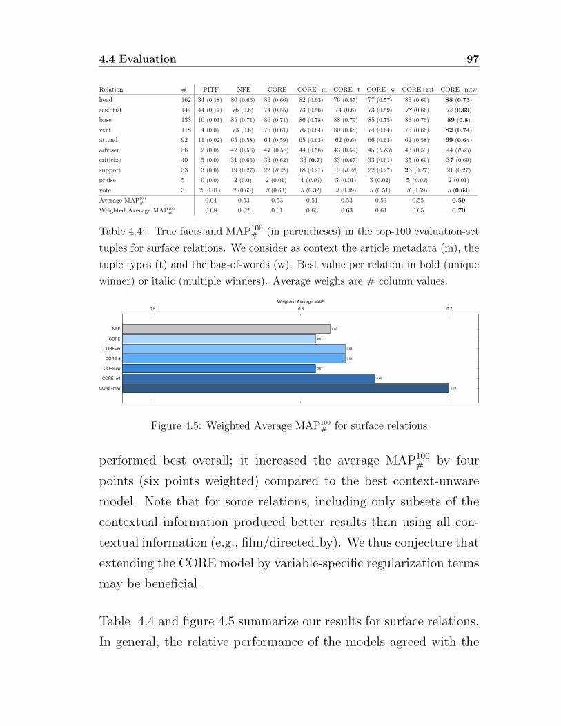
4.4 Evaluation 97
Relation # PITF NFE CORE CORE+m CORE+t CORE+w CORE+mt CORE+mtw
head 162 34 (0.18) 80 (0.66) 83 (0.66) 82 (0.63) 76 (0.57) 77 (0.57) 83 (0.69) 88 (0.73)
scientist 144 44 (0.17) 76 (0.6) 74 (0.55) 73 (0.56) 74 (0.6) 73 (0.59) 78 (0.66) 78 (0.69)
base 133 10 (0.01) 85 (0.71) 86 (0.71) 86 (0.78) 88 (0.79) 85 (0.75) 83 (0.76) 89 (0.8)
visit 118 4 (0.0) 73 (0.6) 75 (0.61) 76 (0.64) 80 (0.68) 74 (0.64) 75 (0.66) 82 (0.74)
attend 92 11 (0.02) 65 (0.58) 64 (0.59) 65 (0.63) 62 (0.6) 66 (0.63) 62 (0.58) 69 (0.64)
adviser 56 2 (0.0) 42 (0.56) 47 (0.58) 44 (0.58) 43 (0.59) 45 (0.63) 43 (0.53) 44 (0.63)
criticize 40 5 (0.0) 31 (0.66) 33 (0.62) 33 (0.7) 33 (0.67) 33 (0.61) 35 (0.69) 37 (0.69)
support 33 3 (0.0) 19 (0.27) 22 (0.28) 18 (0.21) 19 (0.28) 22 (0.27) 23 (0.27) 21 (0.27)
praise 5 0 (0.0) 2 (0.0) 2 (0.01) 4 (0.03) 3 (0.01) 3 (0.02) 5 (0.03) 2 (0.01)
vote 3 2 (0.01) 3 (0.63) 3 (0.63) 3 (0.32) 3 (0.49) 3 (0.51) 3 (0.59) 3 (0.64)
Average MAP100
# 0.04 0.53 0.53 0.51 0.53 0.53 0.55 0.59
Weighted Average MAP100
# 0.08 0.62 0.61 0.63 0.63 0.61 0.65 0.70
Table 4.4: True facts and MAP100# (in parentheses) in the top-100 evaluation-set
tuples for surface relations. We consider as context the article metadata (m), the
tuple types (t) and the bag-of-words (w). Best value per relation in bold (unique
winner) or italic (multiple winners). Average weighs are # column values.
0.5 0.6 0.7
NFE
CORE
CORE+m
CORE+t
CORE+w
CORE+mt
CORE+mtw
Weighted Average MAP
0.62
0.61
0.63
0.63
0.61
0.65
0.70
Figure 4.5: Weighted Average MAP100
# for surface relations
performed best overall; it increased the average MAP100# by four
points (six points weighted) compared to the best context-unware
model. Note that for some relations, including only subsets of the
contextual information produced better results than using all con-
textual information (e.g., film/directed by). We thus conjecture that
extending the CORE model by variable-specific regularization terms
may be beneficial.
Table 4.4 and figure 4.5 summarize our results for surface relations.
In general, the relative performance of the models agreed with the

98 4. Context-Aware Matrix Completion
Figure 4.6: Some facts predicted by the CORE+mtw model for the Freebase
relation author(x,y) and the surface relation “scientist at”(x,y). Most similar
relations also reported, using cosine similarity between the corresponding latent
feature vectors as distance.
one on Freebase relations. One difference is that using bag-of-word
context significantly boosted prediction performance. One reason for
this boost is that related surface relations often share semantically
related words (e.g., “professor at” and “scientist at”) and may occur
in similar sentences (e.g., mentioning “university”, “research”, ...).
Anecdotal results. Fig. 4.6 shows the top test-set predictions of
CORE+mtw for the author and “scientist at” relations. In both
cases, we also list relations that have a similar semantic represen-
tation in the CORE model (highest cosine similarity). Note that

4.5 Summary 99
semantic similarity of relations is one aspect of the model; predic-
tions incorporate other aspects such as context (i.e., two “similar”
relations in different contexts are treated differently).
Training time. We used a machine with 16-cores Intel Xeon proces-
sor and 128GB of memory. Training CORE took roughly one hour,
NFE roughly six hours (single core only), and training CORE+mtw
took roughly 20 hours. Our implementation can handle reasonably
large data, but an investigation of faster, more scalable training
methods appears worthwhile.
4.5 Summary
Context-aware matrix completion aims at integrating additional in-
formation inside the model, in order to increase the overall predic-
tion performance. In this chapter we presented current solutions for
this task, and extended them in order to work in those settings in
which only positive observations are present in input, using relation
extraction as application scenario.
In particular, we presented CORE, a matrix completion model for
open relation extraction that incorporates contextual information.
Our model is based on factorization machines and the open-world
assumption, integrates various forms of contextual information, and
is extensible, i.e., additional contextual information can be inte-
grated when available. Our experimental study on a large real-world
dataset indicates that CORE has significantly better prediction per-
formance than state-of-the-art relation extraction approaches when
contextual information is available.

100 4. Context-Aware Matrix Completion
CHAPTER 5
Conclusion and Outlook
Prediction is very difficult, especially about the future.
Niels Bohr
In this thesis, we addressed efficient solutions for large-scale matrix
completion problems based on latent factor models. We worked over
two lines, respectively tackling the scalability of such solutions and
their prediction quality.
To handle large-scale instances of the matrix completion problem,
asynchronous algorithms based on latent factor models have been
proposed. Such solutions distribute the input over a cluster of
computing nodes, that can communicate asynchronously, and then
perform the training procedure in a distributed fashion. In order
to achieve a fast execution time, a key challenge is to minimize
the communication between computing nodes while balancing the
102 5. Conclusion and Outlook
workload. With this aim, we proposed GASGD, a variant of the
asynchronous stochastic gradient descend algorithm that represents
the data matrix as a graph. This allows GASGD to make use of
graph partitioning algorithms for the distributed placement of the
input. As partitioning solution, we proposed HDRF, a novel vertex-
cut stream-based graph partitioning algorithm that exploits a com-
mon characteristic of real graphs to improve the performance, that is
their power-law degree distribution. The distributed matrix comple-
tion procedure is more scalable when using HDRF to partition the
input data, since it experiments less data overlap among the com-
puting nodes, hence the communication in the system is reduced. It
is also more efficient, since computing nodes receive almost perfectly
equal slices of the input to process. Our empirical studies on real
and synthetic datasets showed the effectiveness of this approach, in
that the distributed asynchronous stochastic gradient descent algo-
rithm proved to converge and run faster when using HDRF as input
partitioner. We also provided a theoretical study for the HDRF
algorithm and an analysis of its behavior when applied on general
graph computation algorithms.
Several studies have shown that feeding the algorithm with more
data might be beneficial for the overall prediction quality of the sys-
tem. To further improve the performance, it is necessary to some-
how incorporate contextual information inside the model, that helps
(even as humans) the refining of the input data. However incorpo-
rating such information in the model, especially when the system
detects only positive evidence in input, that is when the revealed
entries in the data matrix have all the same value, is a challenging
103
task. We proposed a latent factor based matrix completion model
than can exploit contextual information even in the above case, using
as prototypical application scenario a popular natural language pro-
cessing task: relation extraction. In particular, we proposed CORE,
a novel context-aware matrix completion solution for open relation
extraction. Our model takes in input real-word facts from several
sources, such as natural language text and knowledge bases, together
with the context (e.g., the metadata of the newspaper article, the
entity types, the words in the sentence) in which such facts have
been extracted. We showed how to represent facts and relative con-
textual information employing an extended factorization machine
model, that, differently from the original version, also works with
positive only observations, under the open-world assumption. We
discussed an efficient and parallel method for parameter estimation
based on the Bayesian personalized ranking optimization criterion.
Our experimental study on a real-world dataset validated the useful-
ness of contextual data in open relation extraction tasks; our CORE
model provided higher prediction performance than state-of-the-art
solutions.
We believe that the contributions presented have the potential of
large practical applicability. The whole code used in the experi-
ments has been released under the GPLv3 open source license and
is available at https://github.com/fabiopetroni. Moreover, an
implementation of our HDRF partitioning algorithm has been inte-
grated inside GraphLab, a popular graph-based, high performance,
distributed computation framework.
104 5. Conclusion and Outlook
5.1 Future Work
We list some interesting directions for future research, dividing them
in improvements that can be made to our methods and open research
problems.
5.1.1 Improvements
We didn’t investigate efficient implementations for our HDRF algo-
rithm. Currently the algorithm, when processing an incoming edge,
computes a score associated with each partition and selects the one
with the largest value for it. We believe that some optimizations can
be made to speed up the partitioning. For instance, the algorithm
could check if the two vertices already share a partition before com-
puting all scores, and maintain an incrementally updated balance
factor in memory.
We conjecture that introducing a specific regularization term for
each variables group in the CORE model, automatically updated
during the learning procedure on a disjoint validation set, may in-
crease the overall prediction quality. In fact, the CORE model is
composed of several groups of variables, each with its peculiar pre-
dictive power. For instance, the group containing entity types might
carry more information than the group containing articles metadata
for the task of extracting new facts for a specific relation, and this
should be reflected in the associated regularization terms.

5.1 Future Work 105
5.1.2 Open research problems
An open research problem is how to distribute the training proce-
dure for context-aware matrix completion algorithms. For instance,
factorization machines are designed to work on a single core. We pro-
vided a lock-free solution to parallelize the training procedure among
multiple processing cores working on shared memory. Exploring the
feasibility of distributed solutions, able to work in a shared-nothing
environment, is an interesting line of research. One possible ap-
proach could be an asynchronous restyling of the algorithm, where
computing nodes work on a local copy of the data and synchronize
periodically. In this case, however, the input data placement is very
challenging, since the data can’t be represented anymore as a graph
but as an hypergraph. In fact, each training point (an hyperedge)
connects several objects (vertices), e.g., relations, tuples, entities
and several contextual information in the open relation extraction
application scenario.
Another interesting investigation, connected with the previous point,
is concerned with the adaptation of the HDRF graph partitioning
algorithm to hypergraphs. The goal should always be (1) to mini-
mize the vertex replication and (2) to balance the hyperedge load.
We suppose that, also in this case, high degree vertices play a crucial
role for the final quality of the partitioning.
A further line for future research might be the investigation of dis-
tributed solutions for the Bayesian personalized ranking optimiza-
tion criterion. We remark that in a distributed shared-nothing envi-
ronment each computing node has just a partial view on the entire
106 5. Conclusion and Outlook
input data. This setting is compliant, for instance, with the regular-
ized square loss optimization criterion, where each update depend on
a single training point included in the partial view. The Bayesian
personalized ranking criterion, instead, requires the sampling of a
negative counterpart for each given training point, that might not
be present in the partial view of a computing node. A straightfor-
ward solution might, for instance, force the sampling procedure to
draw only from the local portion of the dataset the current com-
puting node owns. Some interesting questions in this regard are:
does this affect the final quality of the algorithm? If yes, which
countermeasures can be put in place?
Finally, scalable version of factorization machines and the BPR cri-
terion might be composed to create a distributed matrix completion
algorithm able to handle those cases in which only positive evidence
exists in input.

Bibliography
[1] G. Adomavicius and A. Tuzhilin. Toward the next genera-
tion of recommender systems: A survey of the state-of-the-art
and possible extensions. IEEE Transactions on Knowledge and
Data Engineering, 17(6):734–749, 2005.
[2] G. Adomavicius and A. Tuzhilin. Context-aware recommender
systems. In Recommender systems handbook, pages 217–253.
Springer, 2011.
[3] A. Ahmed, N. Shervashidze, S. Narayanamurthy, V. Josifovski,
and A. J. Smola. Distributed large-scale natural graph factor-
ization. In Proceedings of the 22nd international conference on
World Wide Web, 2013.
[4] A. Akbik, L. Visengeriyeva, P. Herger, H. Hemsen, and
A. Loser. Unsupervised discovery of relations and discrimi-
native extraction patterns. In Proceedings of the 24th Interna-
tional Conference on Computational Linguistics (COLING),
pages 17–32, 2012.

108 BIBLIOGRAPHY
[5] R. Albert, H. Jeong, and A.-L. Barabasi. Error and attack
tolerance of complex networks. Nature, 406(6794):378–382,
2000.
[6] X. Amatriain. Recommender systems lecture, machine learn-
ing summer school (mlss) 2014. url: https://youtu.be/
bLhq63ygoU8.
[7] K. Andreev and H. Racke. Balanced graph partitioning. In
Proceedings of the 16th Annual ACM Symposium on Paral-
lelism in Algorithms and Architectures, 2004.
[8] S. Auer, C. Bizer, G. Kobilarov, J. Lehmann, R. Cyganiak, and
Z. Ives. Dbpedia: A nucleus for a web of open data. Springer,
2007.
[9] S. Auer, J. Demter, M. Martin, and J. Lehmann. Lodstats–an
extensible framework for high-performance dataset analytics.
In Knowledge Engineering and Knowledge Management, pages
353–362. Springer, 2012.
[10] R. Baeza-Yates, B. Ribeiro-Neto, et al. Modern information
retrieval, volume 463. ACM press New York, 1999.
[11] M. Banko, M. J. Cafarella, S. Soderl, M. Broadhead, and
O. Etzioni. Open information extraction from the web. In
Proceedings of the 20th International Joint Conference on Ar-
tificial Intelligence (IJCAI), 2007.
[12] J. Bennett and S. Lanning. The netflix prize. In Proceedings
of KDD cup and workshop, 2007.

BIBLIOGRAPHY 109
[13] D. Billsus and M. J. Pazzani. Learning collaborative informa-
tion filters. In ICML, volume 98, pages 46–54, 1998.
[14] D. M. Blei, A. Y. Ng, and M. I. Jordan. Latent dirichlet
allocation. the Journal of machine Learning research, 3:993–
1022, 2003.
[15] P. Boldi, M. Rosa, M. Santini, and S. Vigna. Layered la-
bel propagation: A multiresolution coordinate-free ordering
for compressing social networks. In Proceedings of the 20th
international conference on World Wide Web, 2011.
[16] P. Boldi and S. Vigna. The webgraph framework i: compres-
sion techniques. In Proceedings of the 13th international con-
ference on World Wide Web, 2004.
[17] K. Bollacker, C. Evans, P. Paritosh, T. Sturge, and J. Taylor.
Freebase: a collaboratively created graph database for struc-
turing human knowledge. In Proceedings of the 2008 ACM
SIGMOD international conference on Management of data,
pages 1247–1250. ACM, 2008.
[18] O. Bousquet and L. Bottou. The tradeoffs of large scale learn-
ing. In Advances in neural information processing systems,
pages 161–168, 2008.
[19] J. S. Breese, D. Heckerman, and C. Kadie. Empirical analysis
of predictive algorithms for collaborative filtering. In Proceed-
ings of the Fourteenth conference on Uncertainty in artificial
intelligence, pages 43–52. Morgan Kaufmann Publishers Inc.,
1998.

110 BIBLIOGRAPHY
[20] D. S. Callaway, M. E. Newman, S. H. Strogatz, and D. J.
Watts. Network robustness and fragility: Percolation on ran-
dom graphs. Physical review letters, 85(25):5468, 2000.
[21] E. J. Candes and B. Recht. Exact matrix completion via con-
vex optimization. Foundations of Computational mathematics,
9(6):717–772, 2009.
[22] K.-W. Chang, W.-t. Yih, B. Yang, and C. Meek. Typed ten-
sor decomposition of knowledge bases for relation extraction.
In Proceedings of the 2014 Conference on Empirical Methods
in Natural Language Processing (EMNLP), pages 1568–1579,
2014.
[23] K. Chen, T. Chen, G. Zheng, O. Jin, E. Yao, and Y. Yu.
Collaborative personalized tweet recommendation. In Proceed-
ings of the 35th international ACM SIGIR conference on Re-
search and development in information retrieval, pages 661–
670. ACM, 2012.
[24] A. L. Chistov and D. Y. Grigor’ev. Complexity of quantifier
elimination in the theory of algebraically closed fields. In Math-
ematical Foundations of Computer Science 1984, pages 17–31.
Springer, 1984.
[25] D. Cohen, D. Skillicorn, S. Gatehouse, and I. Dalrymple. Sig-
nature detection in geochemical data using singular value de-
composition and semi-discrete decomposition. In 21st Inter-
national Geochemical Exploration Symposium (IGES), 2003.

BIBLIOGRAPHY 111
[26] R. Cohen, K. Erez, D. Ben-Avraham, and S. Havlin. Resilience
of the internet to random breakdowns. Physical review letters,
85(21):4626, 2000.
[27] R. Cohen, K. Erez, D. Ben-Avraham, and S. Havlin. Break-
down of the internet under intentional attack. Physical review
letters, 86(16):3682, 2001.
[28] R. Cyganiak and A. Jentzsch. The linking open data cloud
diagram. url: http://lod-cloud.net.
[29] A. S. Das, M. Datar, A. Garg, and S. Rajaram. Google news
personalization: scalable online collaborative filtering. In Pro-
ceedings of the 16th international conference on World Wide
Web, pages 271–280. ACM, 2007.
[30] O. L. de Lacalle and M. Lapata. Unsupervised relation ex-
traction with general domain knowledge. In Proceedings of the
2013 Conference on Empirical Methods in Natural Language
Processing (EMNLP), pages 415–425, 2013.
[31] J. Dean, G. Corrado, R. Monga, K. Chen, M. Devin, Q. V.
Le, M. Z. Mao, M. Ranzato, A. W. Senior, P. A. Tucker, et al.
Large scale distributed deep networks. In Conference on Neu-
ral Information Processing Systems, 2012.
[32] L. Del Corro and R. Gemulla. Clausie: clause-based open in-
formation extraction. In Proceedings of the 22nd International
Conference on World Wide Web (WWW), 2013.
112 BIBLIOGRAPHY
[33] M. Deshpande and G. Karypis. Item-based top-n recommen-
dation algorithms. ACM Transactions on Information Systems
(TOIS), 22(1):143–177, 2004.
[34] S. N. Dorogovtsev and J. F. Mendes. Evolution of networks.
Advances in physics, 51(4):1079–1187, 2002.
[35] G. Dror, N. Koenigstein, Y. Koren, and M. Weimer. The
yahoo! music dataset and kdd-cup’11. Journal of Machine
Learning Research-Proceedings Track, 18:8–18, 2012.
[36] L. Drumond, S. Rendle, and L. Schmidt-Thieme. Predicting
rdf triples in incomplete knowledge bases with tensor factor-
ization. In Proceedings of the 27th Annual ACM Symposium
on Applied Computing (SAC), 2012.
[37] C. Eaton, D. Deroos, T. Deutsch, G. Lapis, and P. Zikopoulos.
Understanding Big Data. Mc Graw Hill, 2012.
[38] T. Economist. The phone of the future. url: http://www.
economist.com/node/8312260.
[39] M. D. Ekstrand, J. T. Riedl, and J. A. Konstan. Collaborative
filtering recommender systems. Foundations and Trends in
Human-Computer Interaction, 4(2):81–173, 2011.
[40] A. Fader, S. Soderland, and O. Etzioni. Identifying relations
for open information extraction. In Proceedings of the 2011
Conference on Empirical Methods in Natural Language Pro-
cessing (EMNLP), 2011.

BIBLIOGRAPHY 113
[41] M. Fan, D. Zhao, Q. Zhou, Z. Liu, T. F. Zheng, and E. Y.
Chang. Distant supervision for relation extraction with matrix
completion. In Proceedings of the 52nd Annual Meeting of the
Association for Computational Linguistics (ACL), 2014.
[42] U. Feige, M. Hajiaghayi, and J. R. Lee. Improved approxima-
tion algorithms for minimum weight vertex separators. SIAM
Journal on Computing, 38(2):629–657, 2008.
[43] T. Franz, A. Schultz, S. Sizov, and S. Staab. Triplerank: Rank-
ing semantic web data by tensor decomposition. In Proceedings
of the 8th International Semantic Web Conference (ISWC),
2009.
[44] S. Funk. Netflix update: Try this at home. url: http:
//sifter.org/simon/Journal/20061211.html.
[45] R. Gemulla, E. Nijkamp, P. J. Haas, and Y. Sismanis. Large-
scale matrix factorization with distributed stochastic gradient
descent. In Proceedings of the 17th ACM SIGKDD interna-
tional conference on Knowledge discovery and data mining,
2011.
[46] D. Goldberg, D. Nichols, B. M. Oki, and D. Terry. Using
collaborative filtering to weave an information tapestry. Com-
munications of the ACM, 35(12):61–70, 1992.
[47] J. E. Gonzalez, Y. Low, H. Gu, D. Bickson, and C. Guestrin.
Powergraph: Distributed graph-parallel computation on natu-
ral graphs. In Proceedings of the 10th USENIX Symposium on
Operating Systems Design and Implementation (OSDI), 2012.

114 BIBLIOGRAPHY
[48] H. Halberstam and R. Laxton. Perfect difference sets. In Pro-
ceedings of the Glasgow Mathematical Association, 1964.
[49] A. Halevy, P. Norvig, and F. Pereira. The unreasonable effec-
tiveness of data. Intelligent Systems, IEEE, 24(2):8–12, 2009.
[50] T. Hasegawa, S. Sekine, and R. Grishman. Discovering rela-
tions among named entities from large corpora. In Proceedings
of the 42nd Annual Meeting on Association for Computational
Linguistics (ACL), 2004.
[51] J. L. Herlocker, J. A. Konstan, A. Borchers, and J. Riedl. An
algorithmic framework for performing collaborative filtering.
In Proceedings of the 22nd annual international ACM SIGIR
conference on Research and development in information re-
trieval, pages 230–237. ACM, 1999.
[52] T. Hofmann. Latent semantic models for collaborative fil-
tering. ACM Transactions on Information Systems (TOIS),
22(1):89–115, 2004.
[53] Y. Huang, V. Tresp, M. Nickel, A. Rettinger, and H.-P.
Kriegel. A scalable approach for statistical learning in semantic
graphs. Semantic Web, 5(1):5–22, 2014.
[54] N. Jain, G. Liao, and T. L. Willke. Graphbuilder: Scalable
graph etl framework. In 1st International Workshop on Graph
Data Management Experiences and Systems, 2013.
[55] X. Jiang, V. Tresp, Y. Huang, and M. Nickel. Link prediction
in multi-relational graphs using additive models. In Proceed-

BIBLIOGRAPHY 115
ings of the 2012 International Workshop on Semantic Tech-
nologies meet Recommender Systems & Big Data (SeRSy),
2012.
[56] X. Jin, Y. Zhou, and B. Mobasher. Web usage mining based
on probabilistic latent semantic analysis. In Proceedings of the
tenth ACM SIGKDD international conference on Knowledge
discovery and data mining, pages 197–205. ACM, 2004.
[57] U. Kang, C. E. Tsourakakis, and C. Faloutsos. Pegasus: A
peta-scale graph mining system implementation and observa-
tions. In Data Mining, 2009. ICDM’09. Ninth IEEE Interna-
tional Conference on, pages 229–238. IEEE, 2009.
[58] A. Karatzoglou, X. Amatriain, L. Baltrunas, and N. Oliver.
Multiverse recommendation: n-dimensional tensor factoriza-
tion for context-aware collaborative filtering. In Proceedings of
the fourth ACM conference on Recommender systems, pages
79–86. ACM, 2010.
[59] G. Karypis and V. Kumar. A fast and high quality multilevel
scheme for partitioning irregular graphs. SIAM Journal on
scientific Computing, 20(1):359–392, 1998.
[60] M. Kim and K. S. Candan. SBV-Cut: Vertex-cut based graph
partitioning using structural balance vertices. Data & Knowl-
edge Engineering, 72:285–303, 2012.
[61] T. G. Kolda and B. W. Bader. Tensor decompositions and
applications. SIAM review, 51(3):455–500, 2009.

116 BIBLIOGRAPHY
[62] J. A. Konstan, B. N. Miller, D. Maltz, J. L. Herlocker, L. R.
Gordon, and J. Riedl. Grouplens: applying collaborative filter-
ing to usenet news. Communications of the ACM, 40(3):77–87,
1997.
[63] J. A. Konstan and J. Riedl. Recommender systems: from al-
gorithms to user experience. User Modeling and User-Adapted
Interaction, 22(1-2):101–123, 2012.
[64] Y. Koren. Factorization meets the neighborhood: a multi-
faceted collaborative filtering model. In Proceedings of the 14th
ACM SIGKDD international conference on Knowledge discov-
ery and data mining, pages 426–434. ACM, 2008.
[65] Y. Koren. Collaborative filtering with temporal dynamics.
Communications of the ACM, 53(4):89–97, 2010.
[66] Y. Koren, R. Bell, and C. Volinsky. Matrix factorization
techniques for recommender systems. Computer, 42(8):30–37,
2009.
[67] X. Li, G. Cong, X.-L. Li, T.-A. N. Pham, and S. Krish-
naswamy. Rank-geofm: A ranking based geographical fac-
torization method for point of interest recommendation. In
Proceedings of the 38th International ACM SIGIR Conference
on Research and Development in Information Retrieval, pages
433–442. ACM, 2015.
[68] G. Linden, B. Smith, and J. York. Amazon. com recommenda-
tions: Item-to-item collaborative filtering. Internet Comput-
ing, IEEE, 7(1):76–80, 2003.

BIBLIOGRAPHY 117
[69] Y. Low, D. Bickson, J. Gonzalez, C. Guestrin, A. Kyrola, and
J. M. Hellerstein. Distributed graphlab: a framework for ma-
chine learning and data mining in the cloud. Proceedings of
the VLDB Endowment, 5(8):716–727, 2012.
[70] Y. Low, J. Gonzalez, A. Kyrola, D. Bickson, C. Guestrin, and
J. M. Hellerstein. Graphlab: A new framework for parallel
machine learning. In Proceedings of the 26th Conference on
Uncertainty in Artificial Intelligence, 2010.
[71] H. Ma, H. Yang, M. R. Lyu, and I. King. Sorec: social recom-
mendation using probabilistic matrix factorization. In Proceed-
ings of the 17th ACM conference on Information and knowl-
edge management, pages 931–940. ACM, 2008.
[72] H. Ma, T. C. Zhou, M. R. Lyu, and I. King. Improving rec-
ommender systems by incorporating social contextual infor-
mation. ACM Transactions on Information Systems (TOIS),
29(2):9, 2011.
[73] F. Makari, C. Teflioudi, R. Gemulla, P. Haas, and Y. Sisma-
nis. Shared-memory and shared-nothing stochastic gradient
descent algorithms for matrix completion. Knowledge and In-
formation Systems, 42(3):493–523, 2014.
[74] G. Malewicz, M. H. Austern, A. J. Bik, J. C. Dehnert, I. Horn,
N. Leiser, and G. Czajkowski. Pregel: a system for large-scale
graph processing. In Proceedings of the 2010 ACM SIGMOD
International Conference on Management of data, 2010.
118 BIBLIOGRAPHY
[75] J. Mangalindan. Amazon’s recommendation secret. http://
tech.fortune.cnn.com/2012/07/30/amazon-5 CNN Money, 2012.
[76] R. McDonald, K. Hall, and G. Mann. Distributed train-
ing strategies for the structured perceptron. In Human Lan-
guage Technologies: The 2010 Annual Conference of the North
American Chapter of the Association for Computational Lin-
guistics, pages 456–464. Association for Computational Lin-
guistics, 2010.
[77] A. K. Menon and C. Elkan. Link prediction via matrix fac-
torization. In Machine Learning and Knowledge Discovery in
Databases, pages 437–452. Springer, 2011.
[78] B. Min, R. Grishman, L. Wan, C. Wang, and D. Gondek.
Distant supervision for relation extraction with an incomplete
knowledge base. In Proceedings of the 2013 Conference of the
North American Chapter of the Association for Computational
Linguistics: Human Language Technologies (HLT-NAACL),
2013.
[79] B. Min, S. Shi, R. Grishman, and C.-Y. Lin. Ensemble seman-
tics for large-scale unsupervised relation extraction. In Pro-
ceedings of the 2012 Joint Conference on Empirical Methods
in Natural Language Processing and Computational Natural
Language Learning (EMNLP-CoNLL), 2012.
[80] M. Mintz, S. Bills, R. Snow, and D. Jurafsky. Distant super-
vision for relation extraction without labeled data. In Pro-
ceedings of the Joint conference of the 47th Annual Meeting
BIBLIOGRAPHY 119
of the Association for Computational Linguistics and the 4th
International Joint Conference on Natural Language Process-
ing of the Asian Federation of Natural Language Processing
(ACL-IJCNLP), 2009.
[81] A. Mnih and R. Salakhutdinov. Probabilistic matrix factor-
ization. In Advances in neural information processing systems,
pages 1257–1264, 2007.
[82] S. Moghaddam, M. Jamali, and M. Ester. Etf: extended ten-
sor factorization model for personalizing prediction of review
helpfulness. In Proceedings of the fifth ACM international con-
ference on Web search and data mining, pages 163–172. ACM,
2012.
[83] A. Nedic and D. Bertsekas. Convergence rate of incremental
subgradient algorithms. In Stochastic optimization: algorithms
and applications, pages 223–264. Springer, 2001.
[84] A. H. B. News). The age of information overload. url:
http://news.bbc.co.uk/2/hi/programmes/click_online/
9742180.stm.
[85] M. Nickel, V. Tresp, and H.-P. Kriegel. A three-way model for
collective learning on multi-relational data. In Proceedings of
the 28th international conference on machine learning (ICML),
2011.
[86] M. Nickel, V. Tresp, and H.-P. Kriegel. Factorizing yago: scal-
able machine learning for linked data. In Proceedings of the

120 BIBLIOGRAPHY
21st International Conference on World Wide Web (WWW),
2012.
[87] F. Niu, B. Recht, C. Re, and S. J. Wright. Hogwild!: A lock-
free approach to parallelizing stochastic gradient descent. Ad-
vances in Neural Information Processing Systems, 24:693–701,
2011.
[88] Y. Niu, Y. Wang, G. Sun, A. Yue, B. Dalessandro, C. Perlich,
and B. Hamner. The tencent dataset and kdd-cup’12. In KDD-
Cup Workshop, volume 170, 2012.
[89] W. Pan, H. Zhong, C. Xu, and Z. Ming. Adaptive bayesian
personalized ranking for heterogeneous implicit feedbacks.
Knowledge-Based Systems, 73:173–180, 2015.
[90] F. Petroni, L. D. Corro, and R. Gemulla. Core: Context-
aware open relation extraction with factorization machines. In
Proceedings of the 2015 Conference on Empirical Methods in
Natural Language Processing (EMNLP), 2015.
[91] F. Petroni and L. Querzoni. Gasgd: stochastic gradient descent
for distributed asynchronous matrix completion via graph par-
titioning. In Proceedings of the 8th ACM Conference on Rec-
ommender Systems (RecSys), pages 241–248. ACM, 2014.
[92] F. Petroni, L. Querzoni, K. Daudjee, S. Kamali, and G. Ia-
coboni. Hdrf: Stream-based partitioning for power-law graphs.
In Proceedings of the 24th ACM International Conference
on Conference on Information and Knowledge Management
(CIKM), 2015.

BIBLIOGRAPHY 121
[93] Y. C. R. Chen, J. Shi and H. Chen. Powerlyra: Differen-
tiated graph computation and partitioning on skewed graphs.
In Proceedings of the 10th ACM SIGOPS European Conference
on Computer Systems, 2015.
[94] B. Recht and C. Re. Parallel stochastic gradient algorithms
for large-scale matrix completion. Mathematical Programming
Computation, 5(2):201–226, 2013.
[95] B. Recht, C. Re, S. Wright, and F. Niu. Hogwild: A lock-free
approach to parallelizing stochastic gradient descent. In Pro-
ceedings of the 25th Annual Conference on Neural Information
Processing Systems (NIPS), 2011.
[96] S. Rendle. Context-aware ranking with factorization models.
Springer, 2011.
[97] S. Rendle. Factorization machines with libfm. ACM Transac-
tions on Intelligent Systems and Technology (TIST), 3(3):57,
2012.
[98] S. Rendle. Scaling factorization machines to relational data.
In Proceedings of the VLDB Endowment, volume 6, pages 337–
348. VLDB Endowment, 2013.
[99] S. Rendle, C. Freudenthaler, Z. Gantner, and L. Schmidt-
Thieme. Bpr: Bayesian personalized ranking from implicit
feedback. In Proceedings of the 25th Conference on Uncer-
tainty in Artificial Intelligence (UAI), 2009.
[100] S. Rendle, Z. Gantner, C. Freudenthaler, and L. Schmidt-
Thieme. Fast context-aware recommendations with factoriza-

122 BIBLIOGRAPHY
tion machines. In Proceedings of the 34th international ACM
conference on Research and development in Information Re-
trieval (SIGIR), 2011.
[101] S. Rendle and L. Schmidt-Thieme. Pairwise interaction tensor
factorization for personalized tag recommendation. In Proceed-
ings of the third ACM international conference on Web search
and data mining, pages 81–90. ACM, 2010.
[102] P. Resnick, N. Iacovou, M. Suchak, P. Bergstrom, and J. Riedl.
Grouplens: an open architecture for collaborative filtering of
netnews. In Proceedings of the 1994 ACM conference on Com-
puter supported cooperative work, pages 175–186. ACM, 1994.
[103] F. Ricci, L. Rokach, and B. Shapira. Introduction to recom-
mender systems handbook. Springer, 2011.
[104] S. Riedel, L. Yao, A. McCallum, and B. M. Marlin. Relation
extraction with matrix factorization and universal schemas.
In Proceedings of the 2013 Conference of the North Ameri-
can Chapter of the Association for Computational Linguistics:
Human Language Technologies (HLT-NAACL), 2013.
[105] R. Salakhutdinov, A. Mnih, and G. Hinton. Restricted boltz-
mann machines for collaborative filtering. In Proceedings of
the 24th international conference on Machine learning, pages
791–798. ACM, 2007.
[106] M. Saleem. Collaborative filtering: Lifeblood of the social web.
url: http://readwrite.com/2008/06/30/collaborative_
filtering_social_web.

BIBLIOGRAPHY 123
[107] E. Sandhaus. The New York Times Annotated Corpus. Lin-
guistic Data Consortium, Philadelphia, 6(12), 2008.
[108] B. Sarwar, G. Karypis, J. Konstan, and J. Riedl. Application of
dimensionality reduction in recommender system-a case study.
Technical report, DTIC Document, 2000.
[109] B. Sarwar, G. Karypis, J. Konstan, and J. Riedl. Item-based
collaborative filtering recommendation algorithms. In Proceed-
ings of the 10th international conference on World Wide Web,
pages 285–295. ACM, 2001.
[110] B. Schwartz. The paradox of choice: Why more is less. Ecco
New York, 2004.
[111] G. Shani, R. I. Brafman, and D. Heckerman. An mdp-based
recommender system. In Proceedings of the Eighteenth confer-
ence on Uncertainty in artificial intelligence, pages 453–460.
Morgan Kaufmann Publishers Inc., 2002.
[112] Y. Shi, A. Karatzoglou, L. Baltrunas, M. Larson, A. Hanjalic,
and N. Oliver. Tfmap: Optimizing map for top-n context-
aware recommendation. In Proceedings of the 35th interna-
tional ACM SIGIR conference on Research and development
in information retrieval, pages 155–164. ACM, 2012.
[113] Y. Shi, M. Larson, and A. Hanjalic. Exploiting user similarity
based on rated-item pools for improved user-based collabora-
tive filtering. In Proceedings of the third ACM conference on
Recommender systems, pages 125–132. ACM, 2009.
124 BIBLIOGRAPHY
[114] Y. Shi, M. Larson, and A. Hanjalic. Collaborative filtering
beyond the user-item matrix: A survey of the state of the
art and future challenges. ACM Computing Surveys (CSUR),
47(1):3, 2014.
[115] Y. Shinyama and S. Sekine. Preemptive information extrac-
tion using unrestricted relation discovery. In Proceedings of
the 2006 Conference of the North American Chapter of the
Association for Computational Linguistics: Human Language
Technologies (HLT-NAACL), 2006.
[116] A. P. Singh and G. J. Gordon. Relational learning via col-
lective matrix factorization. In Proceedings of the 14th ACM
SIGKDD international conference on Knowledge discovery and
data mining, pages 650–658. ACM, 2008.
[117] A. Singhal. Introducing the knowledge graph: things, not
strings. url: http://googleblog.blogspot.co.uk/2012/05/
introducing-knowledge-graph-things-not.html.
[118] A. Singhal. Modern information retrieval: A brief overview.
IEEE Data Eng. Bull., 24(4):35–43, 2001.
[119] D. Skillicorn. Understanding complex datasets: data mining
with matrix decompositions. CRC press, 2007.
[120] C. Smith. By the numbers: 80+ amazing amazon
statistics. url: http://expandedramblings.com/index.php/
amazon-statistics.

BIBLIOGRAPHY 125
[121] X. Su and T. M. Khoshgoftaar. A survey of collaborative fil-
tering techniques. Advances in Artificial Intelligence, 2009:4,
2009.
[122] M. Surdeanu, J. Tibshirani, R. Nallapati, and C. D. Manning.
Multi-instance multi-label learning for relation extraction. In
Proceedings of the 2012 Joint Conference on Empirical Meth-
ods in Natural Language Processing and Computational Natu-
ral Language Learning (EMNLP-CoNLL), 2012.
[123] G. Takacs, I. Pilaszy, B. Nemeth, and D. Tikk. Scalable col-
laborative filtering approaches for large recommender systems.
The Journal of Machine Learning Research, 10:623–656, 2009.
[124] S. Takamatsu, I. Sato, and H. Nakagawa. Probabilistic ma-
trix factorization leveraging contexts for unsupervised relation
extraction. In Advances in Knowledge Discovery and Data
Mining, pages 87–99. Springer, 2011.
[125] C. Teflioudi, F. Makari, and R. Gemulla. Distributed ma-
trix completion. In International Conference on Data Mining,
2012.
[126] V. Tresp, Y. Huang, M. Bundschus, and A. Rettinger. Ma-
terializing and querying learned knowledge. In Proceedings of
the 2009 International Workshop on Inductive Reasoning and
Machine Learning for the Semantic Web (IRMLeS), 2009.
[127] J. N. Tsitsiklis, D. P. Bertsekas, M. Athans, et al. Dis-
tributed asynchronous deterministic and stochastic gradient

126 BIBLIOGRAPHY
optimization algorithms. IEEE transactions on automatic con-
trol, 31(9):803–812, 1986.
[128] C. Tsourakakis, C. Gkantsidis, B. Radunovic, and M. Vojnovic.
Fennel: Streaming graph partitioning for massive scale graphs.
In Proceedings of the 7th ACM international conference on
Web search and data mining, 2014.
[129] F. Viger and M. Latapy. Efficient and simple generation of ran-
dom simple connected graphs with prescribed degree sequence.
In Computing and Combinatorics. Springer, 2005.
[130] R. West, E. Gabrilovich, K. Murphy, S. Sun, R. Gupta, and
D. Lin. Knowledge base completion via search-based question
answering. In Proceedings of the 23rd international conference
on World wide web, pages 515–526. ACM, 2014.
[131] C. Xie, L. Yan, W.-J. Li, and Z. Zhang. Distributed power-
law graph computing: Theoretical and empirical analysis. In
Advances in Neural Information Processing Systems, 2014.
[132] L. Yao, A. Haghighi, S. Riedel, and A. McCallum. Structured
relation discovery using generative models. In Proceedings of
the 2011 Conference on Empirical Methods in Natural Lan-
guage Processing (EMNLP), pages 1456–1466, 2011.
[133] J. Zhang and P. Pu. A recursive prediction algorithm for col-
laborative filtering recommender systems. In Proceedings of the
2007 ACM conference on Recommender systems, pages 57–64.
ACM, 2007.
127
[134] Y. Zhen, W.-J. Li, and D.-Y. Yeung. Tagicofi: tag informed
collaborative filtering. In Proceedings of the third ACM con-
ference on Recommender systems, pages 69–76. ACM, 2009.
[135] V. W. Zheng, Y. Zheng, X. Xie, and Q. Yang. Collaborative
location and activity recommendations with gps history data.
In Proceedings of the 19th international conference on World
wide web, pages 1029–1038. ACM, 2010.
[136] Y. Zhuang, W.-S. Chin, Y.-C. Juan, and C.-J. Lin. A fast
parallel sgd for matrix factorization in shared memory systems.
In Proceedings of the 7th ACM conference on Recommender
systems, 2013.
[137] P. Zigoris and Y. Zhang. Bayesian adaptive user profiling with
explicit & implicit feedback. In Proceedings of the 15th
ACM international conference on Information and knowledge
management, pages 397–404. ACM, 2006.


