Midterm Exam Solutions

CS 682: Computer Vision (J. Kosecka)

April 13, 2004

HONOR SYSTEM: This examination is strictly individual. You are not allowed to talk, discuss,exchange solutions, etc., with other fellow students. Furthermore, you are only allowed to use the book andyour class notes. You may only ask questions to the class instructor. Any violation of the honor system,or any of the ethic regulations, will be immediately reported according to George Mason University honorcourt.

1. (15) Filtering. The image below is an image of a 3 pixel thick vertical line.

(a) Show the resulting image obtained after convolution of the original with the following approx-imation of the derivative filter [−1, 0, 1] in the horizontal direction. How many local maximaof the filter response do you obtain ?0 0 0 1 1 1 0 0 00 0 0 1 1 1 0 0 00 0 0 1 1 1 0 0 00 0 0 1 1 1 0 0 00 0 0 1 1 1 0 0 00 0 0 1 1 1 0 0 00 0 0 1 1 1 0 0 00 0 0 1 1 1 0 0 00 0 0 1 1 1 0 0 0

Solution The response of each row after convolution with the above filter will be

0 0 1 1 0 −1 −1 0 0

There are two local extrema at 1 and -1.

(b) Suggest a filter which when convolved with the same image would yield a single maximum inthe middle of the line. Demonstrate the result of the convolution on the original image.

0 0 0 1 1 1 0 0 00 0 0 1 1 1 0 0 00 0 0 1 1 1 0 0 00 0 0 1 1 1 0 0 00 0 0 1 1 1 0 0 00 0 0 1 1 1 0 0 00 0 0 1 1 1 0 0 00 0 0 1 1 1 0 0 00 0 0 1 1 1 0 0 0

Solution Convolving the image with the following filter will yield single maximum in themiddle of the line g = [1, 2, 1]T .

(c) What is a difference between Gaussian smoothing and median filtering? How would you decideto use one vs. another ?

Median filter is more used for noise removal, more suitable for salt and pepper noise. Gaussianis used for smoothing and its better when the noise is not spiky.

1

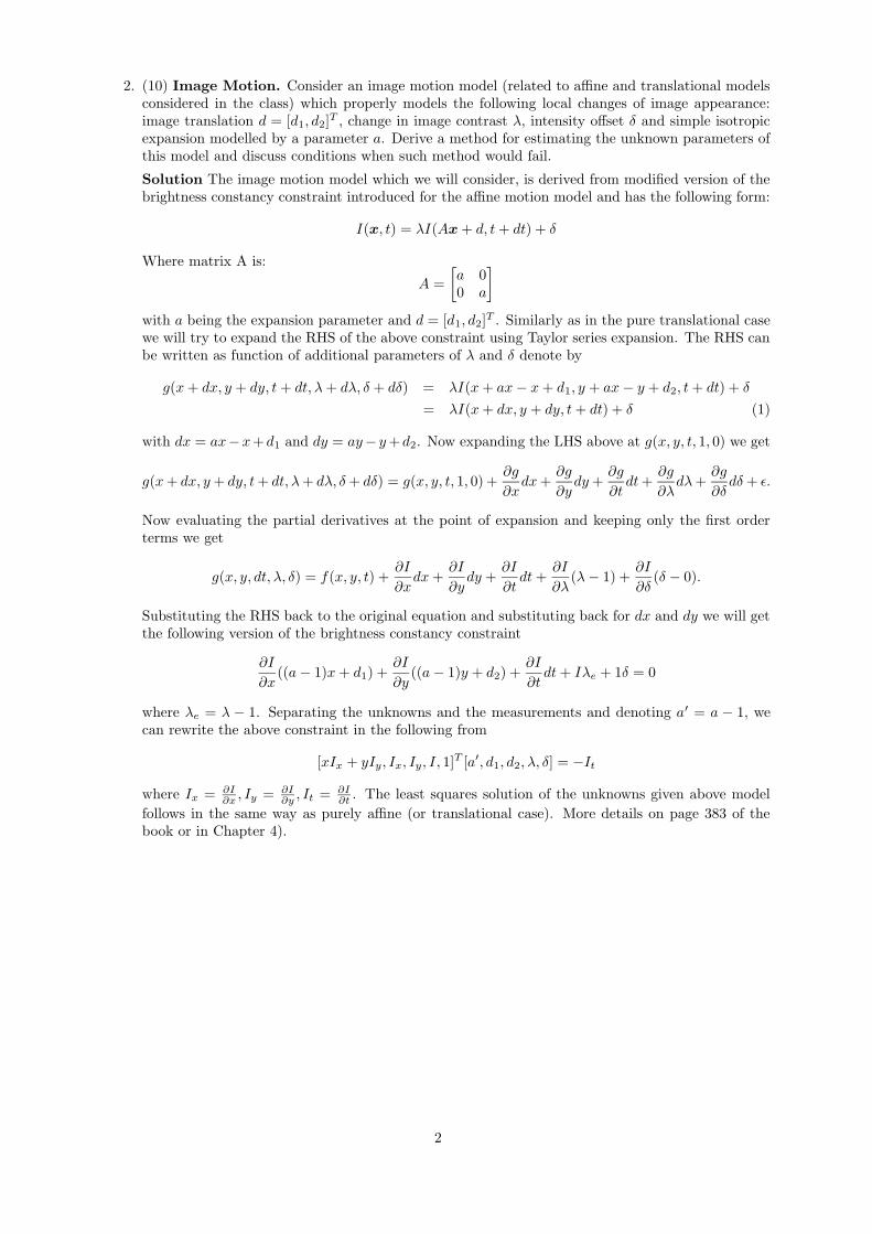
2. (10) Image Motion. Consider an image motion model (related to affine and translational modelsconsidered in the class) which properly models the following local changes of image appearance:image translation d = [d1, d2]

T , change in image contrast λ, intensity offset δ and simple isotropicexpansion modelled by a parameter a. Derive a method for estimating the unknown parameters ofthis model and discuss conditions when such method would fail.

Solution The image motion model which we will consider, is derived from modified version of thebrightness constancy constraint introduced for the affine motion model and has the following form:

I(x, t) = λI(Ax + d, t + dt) + δ

Where matrix A is:

A =

[a 00 a

]

with a being the expansion parameter and d = [d1, d2]T . Similarly as in the pure translational case

we will try to expand the RHS of the above constraint using Taylor series expansion. The RHS canbe written as function of additional parameters of λ and δ denote by

g(x + dx, y + dy, t + dt, λ + dλ, δ + dδ) = λI(x + ax − x + d1, y + ax − y + d2, t + dt) + δ

= λI(x + dx, y + dy, t + dt) + δ (1)

with dx = ax−x+d1 and dy = ay− y +d2. Now expanding the LHS above at g(x, y, t, 1, 0) we get

g(x + dx, y + dy, t + dt, λ + dλ, δ + dδ) = g(x, y, t, 1, 0) +∂g

∂xdx +

∂g

∂ydy +

∂g

∂tdt +

∂g

∂λdλ +

∂g

∂δdδ + ε.

Now evaluating the partial derivatives at the point of expansion and keeping only the first orderterms we get

g(x, y, dt, λ, δ) = f(x, y, t) +∂I

∂xdx +

∂I

∂ydy +

∂I

∂tdt +

∂I

∂λ(λ − 1) +

∂I

∂δ(δ − 0).

Substituting the RHS back to the original equation and substituting back for dx and dy we will getthe following version of the brightness constancy constraint

∂I

∂x((a − 1)x + d1) +

∂I

∂y((a − 1)y + d2) +

∂I

∂tdt + Iλe + 1δ = 0

where λe = λ − 1. Separating the unknowns and the measurements and denoting a′ = a − 1, wecan rewrite the above constraint in the following from

[xIx + yIy, Ix, Iy, I, 1]T [a′, d1, d2, λ, δ] = −It

where Ix = ∂I∂x

, Iy = ∂I∂y

, It = ∂I∂t

. The least squares solution of the unknowns given above model

follows in the same way as purely affine (or translational case). More details on page 383 of thebook or in Chapter 4).

2

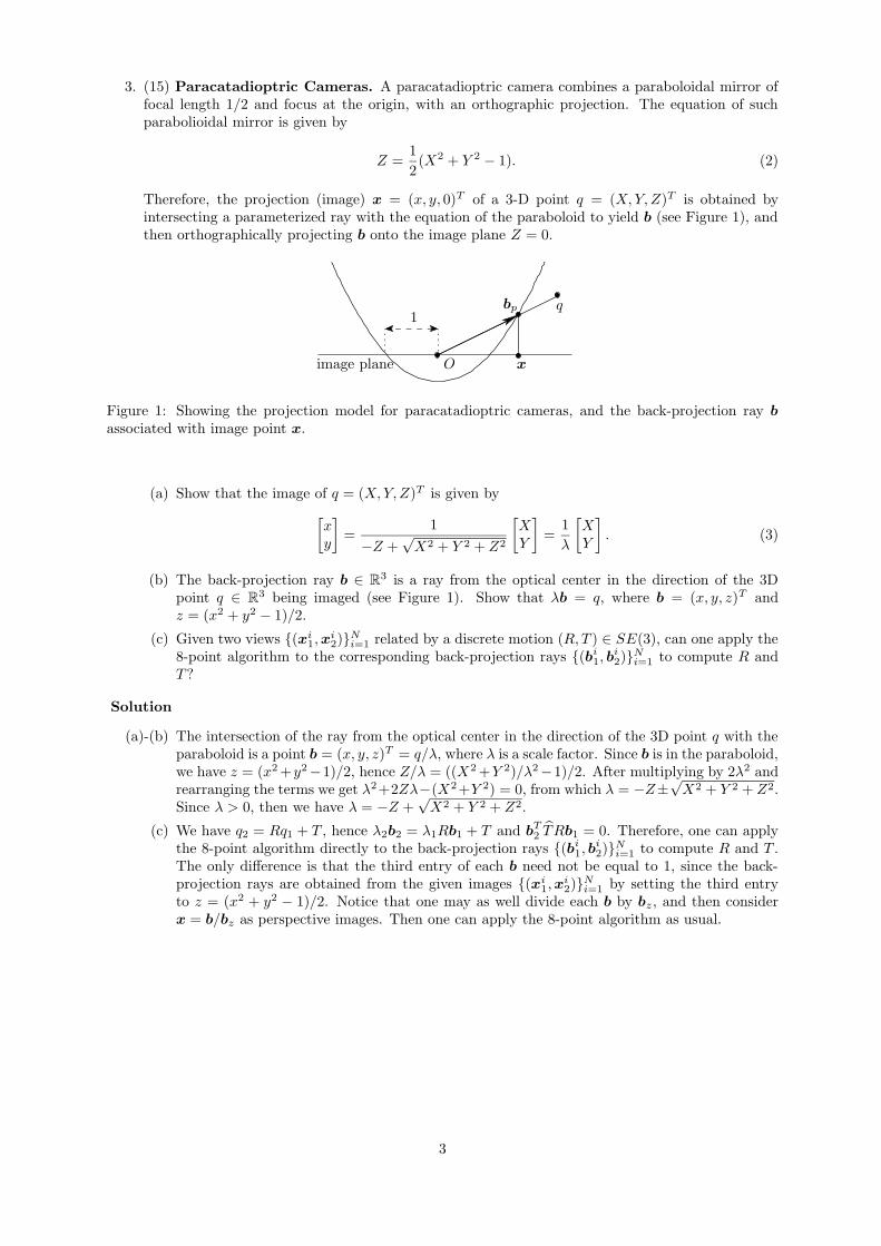
3. (15) Paracatadioptric Cameras. A paracatadioptric camera combines a paraboloidal mirror offocal length 1/2 and focus at the origin, with an orthographic projection. The equation of suchparabolioidal mirror is given by

Z =1

2(X2 + Y 2 − 1). (2)

Therefore, the projection (image) x = (x, y, 0)T of a 3-D point q = (X,Y, Z)T is obtained byintersecting a parameterized ray with the equation of the paraboloid to yield b (see Figure 1), andthen orthographically projecting b onto the image plane Z = 0.

PSfrag replacements

bp

O

q1

ximage plane

Figure 1: Showing the projection model for paracatadioptric cameras, and the back-projection ray b

associated with image point x.

(a) Show that the image of q = (X,Y, Z)T is given by

[xy

]=

1

−Z +√

X2 + Y 2 + Z2

[XY

]=

1

λ

[XY

]. (3)

(b) The back-projection ray b ∈ R3 is a ray from the optical center in the direction of the 3D

point q ∈ R3 being imaged (see Figure 1). Show that λb = q, where b = (x, y, z)T and

z = (x2 + y2 − 1)/2.

(c) Given two views {(xi1,xi

2)}N

i=1related by a discrete motion (R, T ) ∈ SE(3), can one apply the

8-point algorithm to the corresponding back-projection rays {(bi1, bi

2)}N

i=1to compute R and

T?

Solution

(a)-(b) The intersection of the ray from the optical center in the direction of the 3D point q with theparaboloid is a point b = (x, y, z)T = q/λ, where λ is a scale factor. Since b is in the paraboloid,we have z = (x2 +y2−1)/2, hence Z/λ = ((X2 +Y 2)/λ2−1)/2. After multiplying by 2λ2 andrearranging the terms we get λ2+2Zλ−(X2+Y 2) = 0, from which λ = −Z±

√X2 + Y 2 + Z2.

Since λ > 0, then we have λ = −Z +√

X2 + Y 2 + Z2.

(c) We have q2 = Rq1 + T , hence λ2b2 = λ1Rb1 + T and bT2TRb1 = 0. Therefore, one can apply

the 8-point algorithm directly to the back-projection rays {(bi1, bi

2)}N

i=1to compute R and T .

The only difference is that the third entry of each b need not be equal to 1, since the back-projection rays are obtained from the given images {(xi

1,xi

2)}N

i=1by setting the third entry

to z = (x2 + y2 − 1)/2. Notice that one may as well divide each b by bz, and then considerx = b/bz as perspective images. Then one can apply the 8-point algorithm as usual.

3

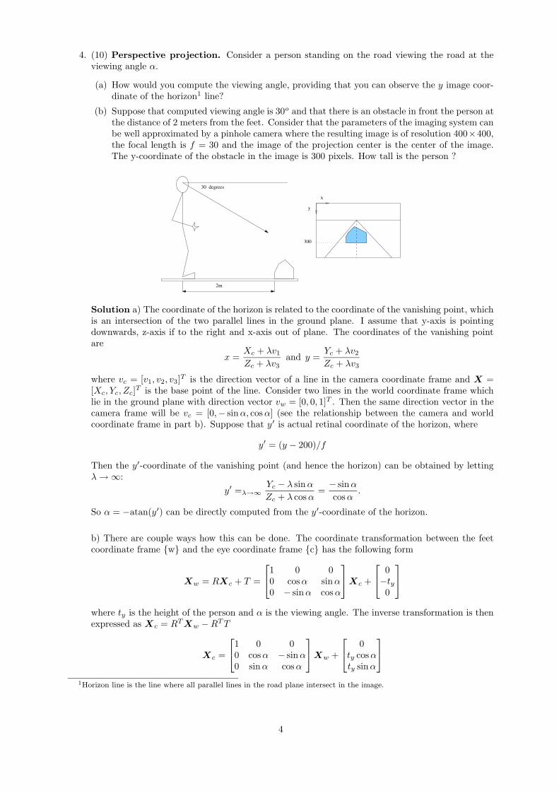
4. (10) Perspective projection. Consider a person standing on the road viewing the road at theviewing angle α.

(a) How would you compute the viewing angle, providing that you can observe the y image coor-dinate of the horizon1 line?

(b) Suppose that computed viewing angle is 30o and that there is an obstacle in front the person atthe distance of 2 meters from the feet. Consider that the parameters of the imaging system canbe well approximated by a pinhole camera where the resulting image is of resolution 400×400,the focal length is f = 30 and the image of the projection center is the center of the image.The y-coordinate of the obstacle in the image is 300 pixels. How tall is the person ?

300

y

x

2m

30 degrees

Solution a) The coordinate of the horizon is related to the coordinate of the vanishing point, whichis an intersection of the two parallel lines in the ground plane. I assume that y-axis is pointingdownwards, z-axis if to the right and x-axis out of plane. The coordinates of the vanishing pointare

x =Xc + λv1

Zc + λv3

and y =Yc + λv2

Zc + λv3

where vc = [v1, v2, v3]T is the direction vector of a line in the camera coordinate frame and X =

[Xc, Yc, Zc]T is the base point of the line. Consider two lines in the world coordinate frame which

lie in the ground plane with direction vector vw = [0, 0, 1]T . Then the same direction vector in thecamera frame will be vc = [0,− sin α, cos α] (see the relationship between the camera and worldcoordinate frame in part b). Suppose that y′ is actual retinal coordinate of the horizon, where

y′ = (y − 200)/f

Then the y′-coordinate of the vanishing point (and hence the horizon) can be obtained by lettingλ → ∞:

y′ =λ→∞

Yc − λ sin α

Zc + λ cos α=

− sin α

cosα.

So α = −atan(y′) can be directly computed from the y′-coordinate of the horizon.

b) There are couple ways how this can be done. The coordinate transformation between the feetcoordinate frame {w} and the eye coordinate frame {c} has the following form

Xw = RXc + T =

1 0 00 cos α sinα0 − sin α cos α

Xc +

0−ty0

where ty is the height of the person and α is the viewing angle. The inverse transformation is thenexpressed as Xc = RT

Xw − RT T

Xc =

1 0 00 cos α − sin α0 sinα cos α

Xw +

0ty cos αty sinα

1Horizon line is the line where all parallel lines in the road plane intersect in the image.

4

Suppose that the coordinate of the obstacle in the feet coordinate system is [Xw, 0, Zw]T , then theretinal y-coordinate y′ (computed as in a) ) is related to its 3D counterpart as

y′ =Yc

Zc

=− sin αZw + cos αtycosαZw + sinαty

.

Since all the above quantities except ty are known we can compute it as

ty =y′ cos αZw + sin αZw

cos α − y′ sin α.

5

5. (15) Rotational motion. Consider set of corresponding points x′

1and x

′

2in pixel coordinates in

two views, which are related by pure rotation R. Assume that all the parameters of the calibrationmatrix K are known except the focal length f . Describe in detail following steps of an algorithmfor recovering R and the focal length of the camera f .

(a) The projection points in two views are related by an unknown 3 × 3 matrix H. Write downthe parametrization of matrix H in terms of rotation matrix entries rij and the focal lengthf .

(b) Describe a linear least squares algorithm for estimation of matrix H. What is the minimalnumber of corresponding points needed in order to solve for H ?

(c) Given the parametrization of H derived in a) describe a method for estimating the actualrotation and the focal length of the camera.

Solution

Rigid body motion equation in case of pure rotation and partial calibration can be written as

λ2x2 = KfRK−1

f λ1x1

where the intrinsic calibration matrix Kf has the following form (the only unknown is the focallength)

Kf =

f 0 00 f 00 0 1

and x1,x2 are the partially calibrated image coordinates (center of the image has beeb subtractedand aspect ration is assumed to be 1). Eliminating the unknown scales λi and denoting H =KfRK−1

f we obtain a following constraint between the measurements and the unknown H:

x2Hx1 = 0

This constraint will give us two linearly independent equations per corresponding pair which canbe written in the form:

a1iHs = 0 (4)

a2iHs = 0 (5)

where Hs = [h11, h12, h13, h21, h22, h23, h31, h32, h33]T is a stacked form of matrix H. Given at least

4 points (two equations each) we can collect all the constraints as rows of matrix A and solve forHs as

AHs = 0

Least squares solution to the above system of homogeneous equations is obtained as eigenvectorassociated with the smallest eigenvalue. Given the least squares solution of Hs, gives us H up to anunknown scale γ. Now given this H we need to recover Kf and R. Note that H has the followingform

H = γ

r11 r12 fr13

r21 r22 fr23

r31/f r32/f r33

Given H the focal length can be then estimated using the constraints between rows of rotationmatrix as rT

1r2 = 0. From this constraint f can be recovered as

f =

√h11h12 + h21h22

−h31h32

.

Given f we can divide the entries h13, h23 by f and multiply the entries h31, h32 by f to eliminatethe unknown focal length factor. The unknown scale γ can be obtained by normalizing the rows ofthe new H (corrected by dividing appropriate entries by f) to be unit norm so as to yield a properrotation matrix.

6

6. (10) 6-point Algorithm for the Recovery of Fundamental (Essential) Matrix. The re-

lationship between a planar homography H and the Fundamental (Essential) matrix F = T ′H(section 5.3.4), suggests a simple alternative algorithm for the recovery of F . Outline the steps ofthe algorithm by assuming that you have available correspondences between at least 4 planar pointsand at least two points which do not lie in the plane. Proceed by first recovering H, followed byT ′.

Solution

First recover the homography H using the 4 planar points. Since xT2Fx1 = 0, we have x

T2T ′Hx1 =

0, hence lT T ′ = 0, where l = x2Hx1. Therefore, one can get the epipole T ′ by taking an intersection

of two epipolar lines l1 and l

2 defined by the two non-planar points in the second view and their

correspondences in the first view warped by homography. That is, T ′ = l2l1. Given H and T ′ the

F becomes F = T ′H.

7