Metrics Programmierung Paralleler und Verteilter Systeme (PPV)
Sommer 2015
Frank Feinbube, M.Sc., Felix Eberhardt, M.Sc., Prof. Dr. Andreas Polze
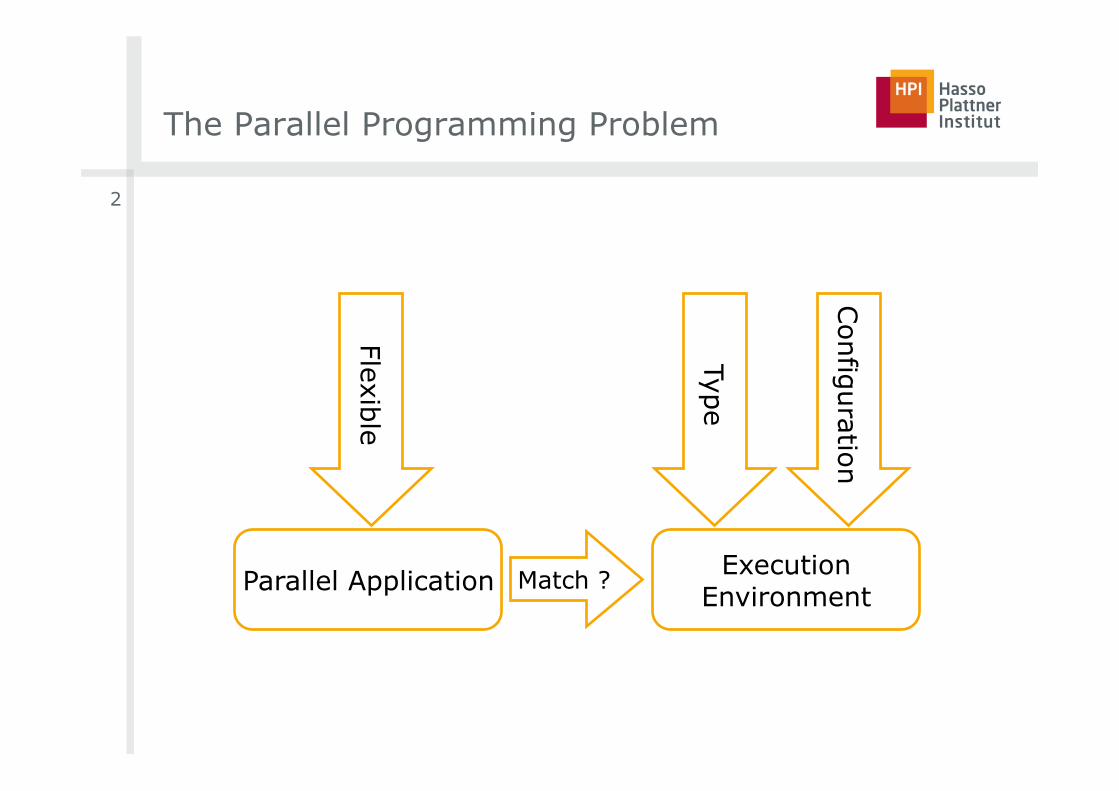
The Parallel Programming Problem
2
Execution Environment Parallel Application Match ?
Configuration
Flexible
Type
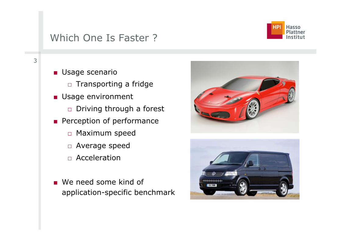
Which One Is Faster ?
■ Usage scenario
□ Transporting a fridge
■ Usage environment
□ Driving through a forest
■ Perception of performance
□ Maximum speed
□ Average speed
□ Acceleration
■ We need some kind of application-specific benchmark
3
Benchmarks
■ Parallelization problems are traditionally speedup problems
■ Traditional focus of high-performance computing
■ Standard Performance Evaluation Corporation (SPEC)
□ SPEC CPU – Measure compute-intensive integer and floating point performance on uniprocessor machines
□ SPEC MPI – Benchmark suite for evaluating MPI-parallel, floating point, compute intense workload
□ SPEC OMP – Benchmark suite for applications using OpenMP
■ NAS Parallel Benchmarks
□ Performance evaluation of HPC systems
□ Developed by NASA Advanced Supercomputing Division
□ Available in OpenMP, Java, and HPF flavours
■ Linpack
Parallel Programming Concepts | 2013 / 1014
4
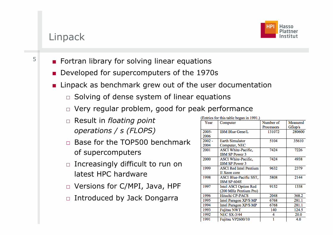
Linpack
■ Fortran library for solving linear equations
■ Developed for supercomputers of the 1970s
■ Linpack as benchmark grew out of the user documentation
□ Solving of dense system of linear equations
□ Very regular problem, good for peak performance
□ Result in floating point operations / s (FLOPS)
□ Base for the TOP500 benchmark of supercomputers
□ Increasingly difficult to run on latest HPC hardware
□ Versions for C/MPI, Java, HPF
□ Introduced by Jack Dongarra
5
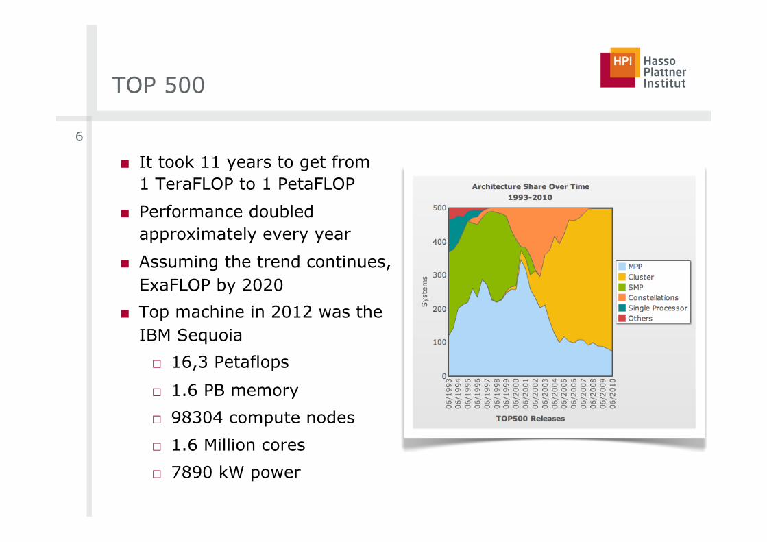
TOP 500
■ It took 11 years to get from 1 TeraFLOP to 1 PetaFLOP
■ Performance doubled approximately every year
■ Assuming the trend continues, ExaFLOP by 2020
■ Top machine in 2012 was the IBM Sequoia
□ 16,3 Petaflops
□ 1.6 PB memory
□ 98304 compute nodes
□ 1.6 Million cores
□ 7890 kW power
6
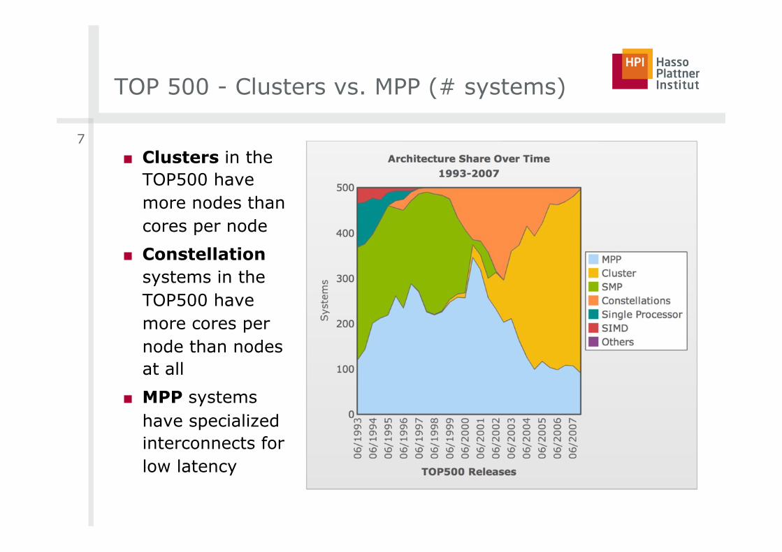
TOP 500 - Clusters vs. MPP (# systems)
■ Clusters in the TOP500 have more nodes than cores per node
■ Constellation systems in the TOP500 have more cores per node than nodes at all
■ MPP systems have specialized interconnects for low latency
7
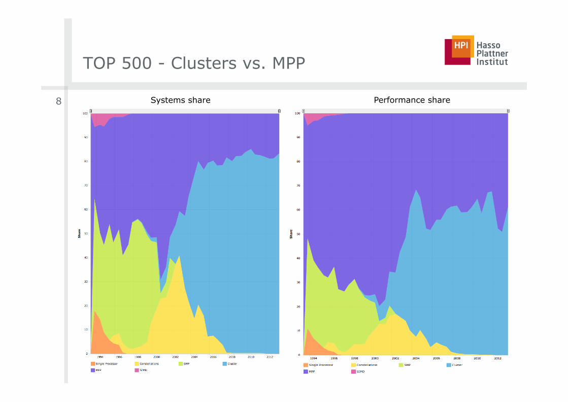
TOP 500 - Clusters vs. MPP
8 Systems share Performance share
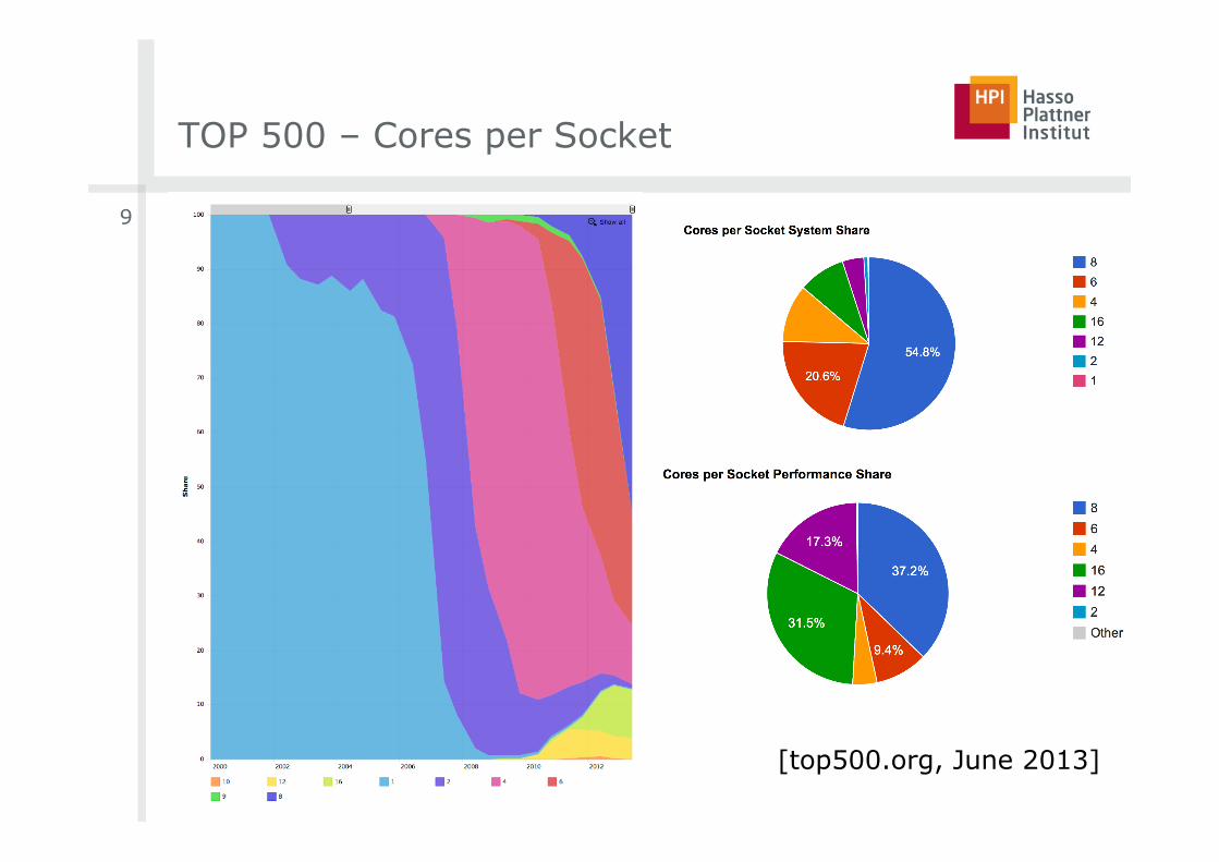
TOP 500 – Cores per Socket
9
[top500.org, June 2013]
Metrics
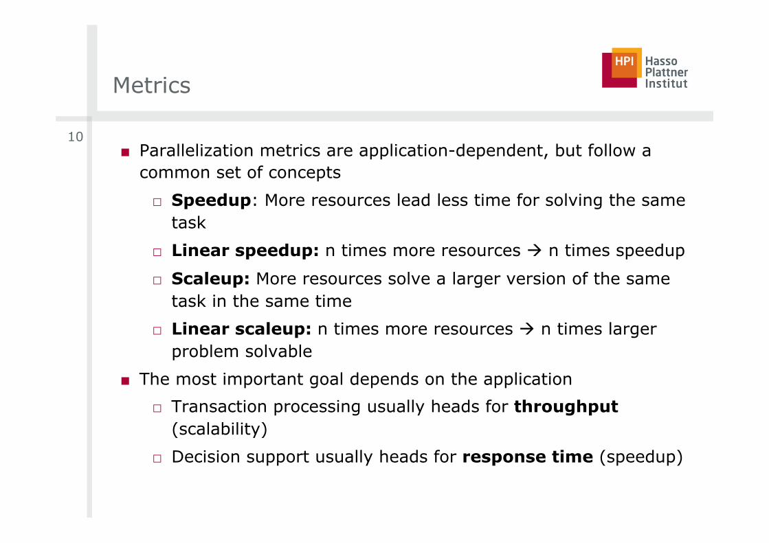
■ Parallelization metrics are application-dependent, but follow a common set of concepts
□ Speedup: More resources lead less time for solving the same task
□ Linear speedup: n times more resources à n times speedup
□ Scaleup: More resources solve a larger version of the same task in the same time
□ Linear scaleup: n times more resources à n times larger problem solvable
■ The most important goal depends on the application
□ Transaction processing usually heads for throughput (scalability)
□ Decision support usually heads for response time (speedup)
10
Speedup
Parallel Programming Concepts | 2013 / 1014
11
Speedup
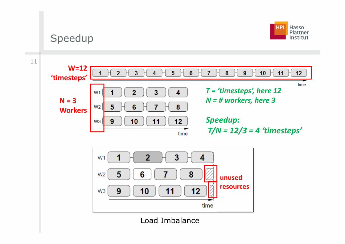
� Consider simple situation: All processing units execute their assigned work in exactly the same amount of time� Solving a problem would take Time T sequentially (1 Worker essentially)� Having N workers solve the problem now ideally only in T/N� This is a speedup of N
Modified from [1] Introduction to High Performance Computing for Scientists and Engineers
T = ‘timesteps’, here 12N = # workers, here 3
Speedup:T/N = 12/3 = 4 ‘timesteps’
N = 3Workers
W=12‘timesteps’
Lecture 2 – Parallelization Fundamentals 19 / 31
Loal Imbalance
� Consider a more realistic situation: Not all workers might execute their tasks in the same amount of time� Reason: The problem simply can not be properly partitioned
into pieces with equal complexity � Nearly worst case: All but a few have nothing to do but wait
for the latecomers to arrive (because of different execution times)
Lecture 2 – Parallelization Fundamentals
Modified from [1] Introduction to High Performance Computing for Scientists and Engineers
unusedresources
� Load imbalance hampers performance, because someresources are underutilized
20 / 31
Load Imbalance
Speedup
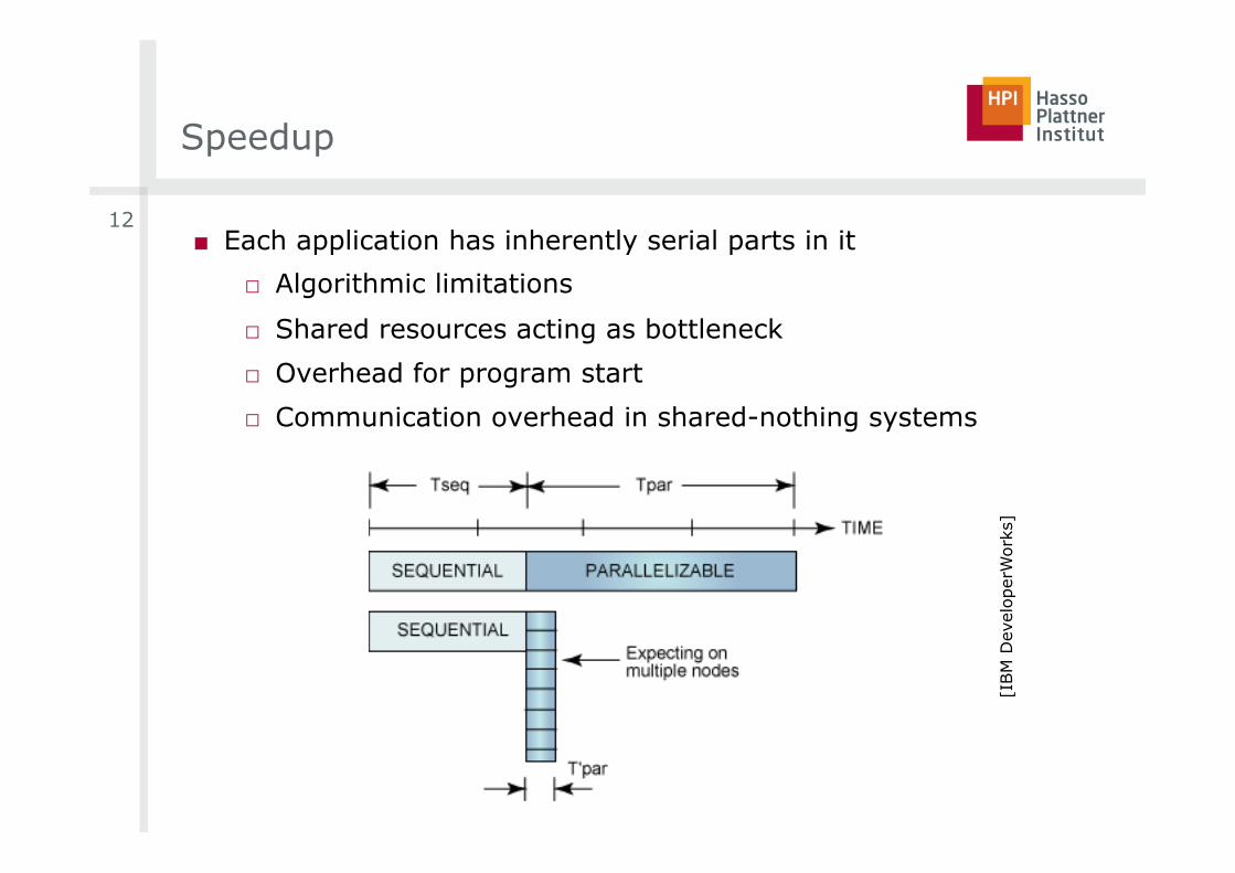
■ Each application has inherently serial parts in it
□ Algorithmic limitations
□ Shared resources acting as bottleneck
□ Overhead for program start
□ Communication overhead in shared-nothing systems
12
[IBM
Dev
elop
erW
orks
]
Amdahl’s Law (1967)
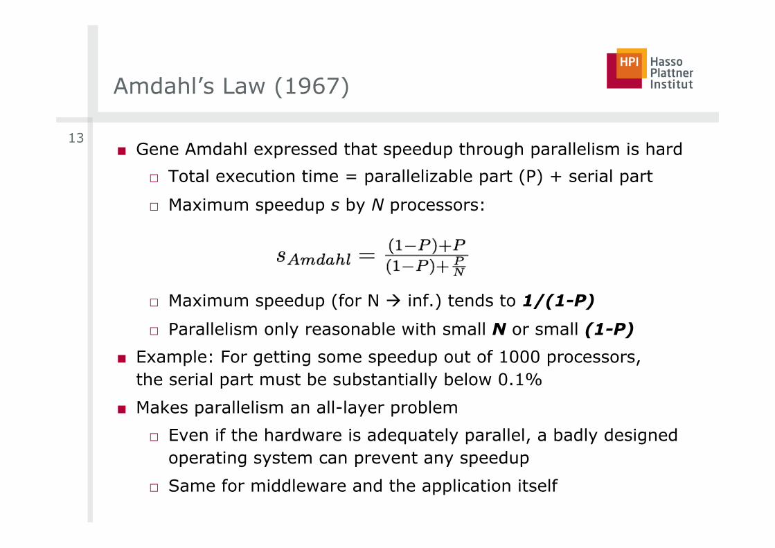
■ Gene Amdahl expressed that speedup through parallelism is hard
□ Total execution time = parallelizable part (P) + serial part
□ Maximum speedup s by N processors:
□ Maximum speedup (for N à inf.) tends to 1/(1-P)
□ Parallelism only reasonable with small N or small (1-P)
■ Example: For getting some speedup out of 1000 processors, the serial part must be substantially below 0.1%
■ Makes parallelism an all-layer problem
□ Even if the hardware is adequately parallel, a badly designed operating system can prevent any speedup
□ Same for middleware and the application itself
13
Amdahl’s Law
14
Amdahl’s Law
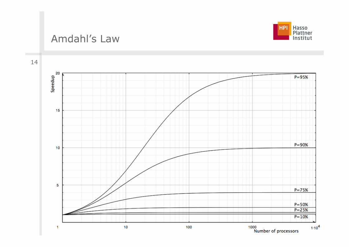
■ 90% parallelizable code leads to not more than speedup by factor 10, regardless of processor count
■ Result: Parallelism is useful for small number of processors, or highly parallelizable code
■ What’s the sense in big parallel / distributed machines?
■ “Everyone knows Amdahl’s law, but quickly forgets it.” [Thomas Puzak, IBM]
■ Relevant assumptions
□ Maximum theoretical speedup is N (linear speedup)
□ Assumption of fixed problem size
□ Only consideration of execution time for one problem
15
Gustafson-Barsis’ Law (1988)
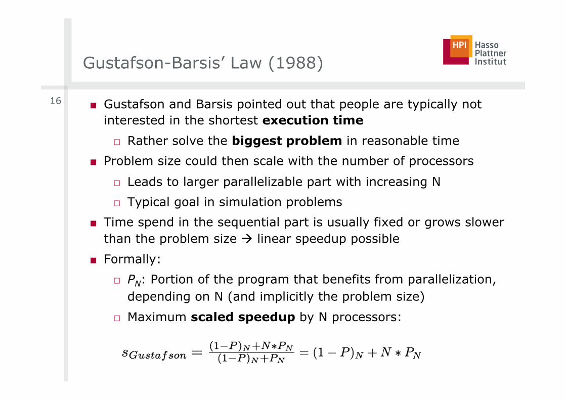
■ Gustafson and Barsis pointed out that people are typically not interested in the shortest execution time
□ Rather solve the biggest problem in reasonable time
■ Problem size could then scale with the number of processors
□ Leads to larger parallelizable part with increasing N
□ Typical goal in simulation problems
■ Time spend in the sequential part is usually fixed or grows slower than the problem size à linear speedup possible
■ Formally:
□ PN: Portion of the program that benefits from parallelization, depending on N (and implicitly the problem size)
□ Maximum scaled speedup by N processors:
16
Karp-Flatt-Metric
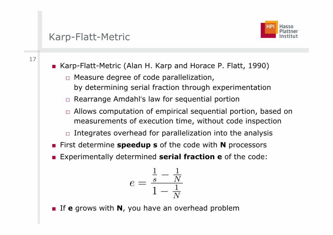
■ Karp-Flatt-Metric (Alan H. Karp and Horace P. Flatt, 1990)
□ Measure degree of code parallelization, by determining serial fraction through experimentation
□ Rearrange Amdahl‘s law for sequential portion
□ Allows computation of empirical sequential portion, based on measurements of execution time, without code inspection
□ Integrates overhead for parallelization into the analysis
■ First determine speedup s of the code with N processors
■ Experimentally determined serial fraction e of the code:
■ If e grows with N, you have an overhead problem
17
e =1s � 1
N
1� 1N
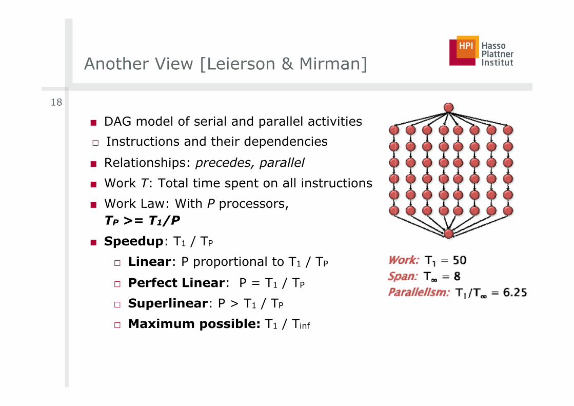
Another View [Leierson & Mirman]
■ DAG model of serial and parallel activities
□ Instructions and their dependencies
■ Relationships: precedes, parallel
■ Work T: Total time spent on all instructions
■ Work Law: With P processors, TP >= T1/P
■ Speedup: T1 / TP
□ Linear: P proportional to T1 / TP
□ Perfect Linear: P = T1 / TP
□ Superlinear: P > T1 / TP
□ Maximum possible: T1 / Tinf
18
Examples
■ Fibonacci function FK+2=FK+FK+1
□ Each computed value depends on earlier one
□ Cannot be obviously parallelized
■ Parallel search
□ Looking in a search tree for a ‚solution‘
□ Parallelize search walk on sub-trees
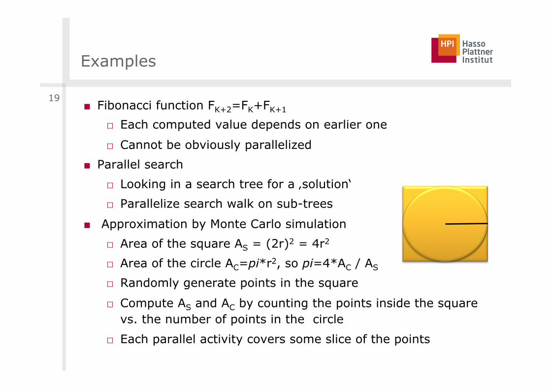
■ Approximation by Monte Carlo simulation
□ Area of the square AS = (2r)2 = 4r2
□ Area of the circle AC=pi*r2, so pi=4*AC / AS
□ Randomly generate points in the square
□ Compute AS and AC by counting the points inside the square vs. the number of points in the circle
□ Each parallel activity covers some slice of the points
19


