
Master-slave Force-reflecting Resolved Motion Control of Hydraulic Mobile Machines
by M i n g Zhu
B . S c , Shanghai Jiao Tong University, China, 1987
A T H E S I S S U B M I T T E D I N P A R T I A L F U L F I L L M E N T O F
T H E R E Q U I R E M E N T S F O R T H E D E G R E E O F
M A S T E R O F A P P L I E D S C I E N C E
in
T H E F A C U L T Y O F G R A D U A T E S T U D I E S
D E P A R T M E N T O F E L E C T R I C A L E N G I N E E R I N G
We accept this thesis as conforming
to the required standard
T H E U N I V E R S I T Y O F B R I T I S H C O L U M B I A
A p r i l 1994
© M i n g Zhu, 1994

In presenting this thesis in partial fulfilment of the requirements for an advanced
degree at the University of British Columbia, I agree that the Library shall make it
freely available for reference and study. I further agree that permission for extensive
copying of this thesis for scholarly purposes may be granted by the head of my
department or by his or her representatives. It is understood that copying or
publication of this thesis for financial gain shall not be allowed without my written
permission.
Department of £ J '& CAY t
The University of British Columbia Vancouver, Canada
DE-6 (2/88)

Abstract
Issues concerning the design and implementation of master-slave force-reflecting resolved
motion control of hydraulic mobile machines are addressed i n this thesis.
Network concepts and linear system theory are used to design and analyze general force-
reflecting teleoperator systems to achieve high performance while maintaining stability. A new
control structure is proposed to achieve "transparency" for teleoperator systems under rate control.
A novel approach to stability analysis of the stiffness feedback strategy proposed i n previous
work is provided which, under certain condition, guarantees global asymptotic stability of the
teleoperator system. The system could be either under rate or position control and could be
subject to time-delays, nonlinearities or active environments.
The closed-form inverse kinematics solutions of an excavator and a feller-buncher, which
are four and five degree-of-freedom manipulators respectively, are provided to achieve resolved-
motion of the manipulator's end-effector.
Using the U B C magnetically levitated joystick, the master-slave force-reflecting resolved
motion control has been successfully implemented on a C A T - 2 1 5 excavator and a CAT-325
feller-buncher. Machine experiments demonstrate the effectiveness of this control strategy i n
improving productivity and safety of general hydraulic mobile machines.
i i

Table of Contents
Abstract i i
List of Tables v i
List of Figures v i i
Acknowledgments x
1 Introduction 1
1.1 Motivation 3
1.2 Previous Work 6
1.3 Thesis Overview 9
2 Resolved Motion 10
2.1 Overview 10
2.2 Inverse Kinematics of an Excavator 12
2.3 Inverse Kinematics of a Feller-buncher 16
2.3.1 Inverse Kinematics: Approach 1 18
2.3.2 Inverse Kinematics: Approach 2 20
2.3.3 Some Comments on the Inverse Kinematics 24
3 Force Reflection 25
3.1 Network Representation of Teleoperator System 26
3.2 General Teleoperator Structure 28
3.3 Force-reflecting Control 32
3.3.1 Coordinating Force 32
i i i

3.3.2 Force Feedback 34
3.4 Transparency 37
3.4.1 Achieving Transparency Under Position Control 37
3.4.2 Achieving Transparency Under Rate Control 43
3.4.3 Achieving Transparency V i a Impedance Identification 48
4 Stiffness Feedback 50
4.1 Principle 50
4.2 Stability 52
5 System Overview 62
5.1 Master — Maglev Joystick 63
5.1.1 System Configuration 64
5.1.2 Sensor and actuator 65
5.1.3 Control about the Remote Center of Compliance 66
5.2 Slave — Hydraulic Mobi le Machines 69
5.3 Computing System . ; 70
6 Machine Experiments 72
6.1 Endpoint Force Sensing 72
6.1.1 Model ing 72
6.1.2 Torque Computations 78
6.1.3 Recursive Least-squares L i n k Parameter Estimation 81
iv

6.2 Excavator Experiments 90
6.2.1 Resolved Mot ion Control 91
6.2.2 Apply ing a Desired Force 96
63 Feller-buncher Experiments 99
6.3.1 Desired Force Tracking 102
6.3.2 Complete Tree Cutting Process 105
6.3.3 Practical Issues 107
7 Conclusions 111
7.1 Thesis Contributions I l l
7.2 Further Work 112
References 113
v

List of Tables
2.1 Excavator l ink Denavit-Hartenberg parameters 13
2.2 Feller-buncher l ink Denavit-Hartenberg parameters 17
6.3 Piston geometry of the excavator 78
6.4 Piston geometry of the feller-buncher 78
6.5 Joint linkage geometry of the excavator 80
6.6 Joint Linkage geometry o f the feller-buncher 80
6.7 Gain selections for the excavator experiments 90
6.8 M a x i m u m feedback force for the excavator experiments 91
6.9 Gain selections for the feller-buncher experiments 99
6.10 M a x i m u m feedback force for the feller-buncher experiments 100
6.11 Detent parameters for the feller-buncher experiments 102
vi

List of Figures
1.1 Kinemaucally similar master-slave system 1
1.2 Kinematically dissimilar master-slave system 2
1.3 Excavator schematic 4
1.4 Photograph of a typical excavator 4
1.5 Feller-buncher schematic . 5
1.6 Photograph of a typical feller-buncher 5
2.7 Excavator configuration 13
2.8 Projection of excavator onto plane 14
2.9 Feller-buncher configuration 16
3.10 Ideal teleoperator system 25
3.11 Network concepts 26
3.12 Network representation of teleoperator system 27
3.13 General teleoperator structure: After Lawrence, 1992 29
3.14 Closed-loop stability analysis 31
3.15 Position-position structure 32
3.16 Network representation of position-position structure 33
3.17 Mechanical equivalence of position-position structure 33
3.18 Rate-position structure 34
3.19 Position-force structure 35
3.20 Intervenient impedance 40
3.21 Achieving transparency under rate control 44
3.22 Achieving transparency v ia parameter identification 49
vii

4.23 Comparison of two rate control structures 50
4.24 Stiffness adjustment scheme 51
4.25 Stiffness feedback control block diagram 52
4.26 Trajectory i n phase plane 57
4.27 Trajectory i n phase plane 58
4.28 Trajectory i n phase plane 60
4.29 Trajectory i n phase plane 61
5.30 Overall system configuration 62
5.31 Maglev Joystick system configuration 64
5.32 Maglev Joystick assembly 65
5.33 Frame assignment 67
5.34 V M E cage configuration 70
6.35 Two-bar mechanical linkage 79
6.36 Four-bar mechanical linkage 79
6.37 Excavator l ink parameter identification 82
6.38 Excavator l ink parameter identification 83
6.39 Excavator l ink parameter identification 84
6.40 Excavator l ink parameter identification 85
6.41 Feller-buncher l ink parameter identification 86
6.42 Feller-buncher l ink parameter identification 87
6.43 Feller-buncher l ink parameter identification 88
6.44 Feller-buncher l ink parameter identification 89
6.45 Excavator resolved motion control: bucket straight up 92
6.46 Excavator resolved motion control: bucket straight down 93
vii i
6.47 Excavator resolved motion control: bucket straight out . . . 94
6.48 Excavator resolved motion control: bucket straight i n 95
6.49 Excavator stiffness control: applying a desired force 97
6.50 Excavator force control: applying a desired force 98
6.51 Detent implementation 100
6.52 Conventional position control 101
6.53 Feller-buncher stiffness control: force tracking 103
6.54 Feller-buncher control without force-reflection: force tracking 104
6.55 Feller-buncher stiffness control: tree cutting process 106
6.56 Feller-buncher step response: boom 108
6.57 Feller-buncher step response: stick 109
6.58 Feller-buncher step response: tilt 110
ix

Acknowledgments
I would l ike to thank my supervisor T i m Salcudean for his support and guidance i n my
thesis work. I wish to thank Peter Lawrence and Dan Chan for their invaluable assistance and
encouragement during the enduring machine experiments. I would also l ike to thank N i a l l Parker
and T i m Vlaar for their helpful discussions and advice.
Special thanks to my wife Jane Zhang for her support and understanding.

Chapter 1 Introduction
Due to the fact that fully autonomous robots could not be realized using the latest technology,
researchers began to concentrate on combining human versatility and expertise with machines.
In some applications such as microsurgery, perhaps it w i l l never be possible to have a robot
acting alone.
The idea of using a master manipulator to command a slave manipulator can be traced back
to the pioneering work by Goertz and his colleagues i n the late 1940s when the first recognizable
mechanical master-slave manipulator was built. Later i n the early 1950s, the electrical servo was
introduced. Most of these early designs exploit a kinematically similar master and slave because
of the simplicity of the required controller, see Figure 1.1. Corresponding joint servos between
the master and slave are tied together through electrical means. A s a result, only position control
i n which the position of the master is interpreted as a position command to the slave, can be used.
Master Manipulator Slave Manipulator
Figure 1.1 Kinematically similar master-slave system
1

Chapter 1: Introduction 2
Later, multi-degree-of-freedom joysticks were used as the input device to command the slave
manipulator (see Figure 1.2). This structure soon gained its popularity due to the fact that the
joystick can be used universally and usually takes less space. Rate control, i n which the position
of the master is interpreted as a velocity command to the slave, combined with conventional
position control can be realized. For example, the space shuttle remote manipulator system is
provided with both position and rate control modes [1]. When the joystick controls the motion
of the endpoint of the slave directly, we call it resolved motion control.
Hand Controller S | ave Manipulator
Figure 1.2 Kinematically dissimilar master-slave system
Contact information is helpful to the operator i n reducing contact force, therefore reducing
damages to the remote object. It also helps an operator probing i n an uncertain environment,
and reduces task completion time. Although this information can be provided by visual display,
the most natural and efficient way is to transmit it directly to the operator's hand. In the case
of multiaxial operation, a visual display is not acceptable to the user. When the contact force
is reflected v ia the master actuator to the operator's hand, the teleoperator system is said to be
controlled bilaterally, and the operator is said to be kinesthetically coupled to the environment.
The early application of teleoperator systems were mainly i n the nuclear industry to remove
radioactive materials without involving the human i n the hazardous environment. The original

Chapter 1: Introduction 3
idea of manipulating objects remotely was soon broadened to include working on a different
power scale, for instance, as a "man-amplifier" [2]. Teleoperator systems have the potential to
play an important role i n future remote or hazardous operations, such as space servicing, undersea
exploration, and mining and i n delicate operations such as microsurgery, microassembly and
microchemistry.
1.1 Motivation
Hydraulic mobile machines can be found in various industries including forestry, mining and
construction. To operate a conventional hydraulic mobile machine such as an excavator (Figure
1.3) or a feller-buncher (Figure 1.5), an operator uses two joysticks to control the individual
displacements of the hydraulic cylinders o f the machine i n an uncoordinated way. In order to
achieve a desired end-effector motion, e.g. a straight line motion, a complicated two-handed
maneuver must be executed. It usually takes a few months to train an operator.
The advantages of applying resolved motion control to these machines are the following:
1. Simple, intuitive, single-hand operation.
2. H i g h performance, since accurate motion, such as a straight line, can be obtained.
3. Reduced machine wear, since unnecessary joint motion is reduced to a minimum.
4. Increased productivity and safety, since the machine moves i n an intuitive way.

Chapter 1: Introduction
Drawing by S. Tafazoli

Chapter I: Introduction 5

Chapter I: Introduction 6
Currently, an experienced operator depends solely on cues such as engine noise and machine
motion to determine its load. H igh contact force can easily cause damage to the task, even to
the machine itself.
The advantages of applying force reflection to the control of these machines are the following:
1. Improved performance, as more delicate tasks can be achieved.
2. Improved safety, since machine tip-over can be avoided by pushing the joystick back to the
center under computer control.
3. Reduced machine wear, as the operator is more able to determine the machine load.
For a detailed description of applications of these hydraulic mobile machines i n construction
and forestry industry, refer to [3].
The application of resolved motion control to general hydraulic machines was first investi
gated by Lawrence et al. [4]. Later, force-reflecting resolved control was applied by Parker [3]
to a three degree-of-freedom log-loader. Our goal i n this project was focusing on the applica
tion of force-reflecting resolved control to a wider variety of machines such as excavators and
feller-bunchers and addressing related issues.
1.2 Previous Work
The first recognizable mechanical master-slave manipulator was built i n the late 1940s by
Goertz and his colleagues. Later i n the early 1950s, an electric servomanipulator system with
force reflection capacity was introduced [5].
A survey on different universal joysticks can be found i n [6].

Chapter 1: Introduction 1
A dissimilar master and slave teleoperator system was studied by Jansen et al. [7] i n which
force-reflection based on the master and slave Jacobians was proposed to control a 7 - D O F slave
manipulator.
A comparison between position and rate control was done by K i m et al. [8]. Position control
is recommended for small workspaces with fast manipulators, while rate control is recommend
for large workspaces with slow manipulators.
The design of force-reflecting teleoperator systems for robot surgery were reported by Sabatini
et al. [9]. A min i six-degree-of-freedom magnetically levitated wrist designed for microsurgery
experiments was designed by Yan [10].
The human dynamics i n response to visual and force feedback was modelled and incorporated
into the controller design and evaluation by Lee et al. [11]. The role of the controller was defined
as modifying the dynamic characteristics of the master and slave arms to achieve a desirable one.
In [12], the force applied by the operator was used locally at the master side to modify its
dynamics so that a "heavier" or a "lighter" master can be easily realized.
Hard contact with direct force feedback was examined by Hannaford et al. [13]. The effect
of the operator i n stabilizing the system was reported as i n much the same manner as local
damping feedback of the hand controller. It was suggested that the human operator impedance
be estimated on-line i n order to find the minimum necessary damping for the system. Salcudean
and Wong [14] added damping which is proportional to the amount of contact force to the system
to maintain hard contact stability, therefore avoiding "sluggishness" during free motion.
Force reflection under time delay was investigated by Spong and Anderson [15], v ia scattering
theory. Stability was achieved by introducing a control law that prevents the communication block
from generating energy. However, L a w n and Hannaford [16] reported a 50% increase of task

Chapter 1: Introduction 8
completion time with these passivity based methods. K i m et al. [17] proposed compliant control
i n which the feedback of the contact force is done locally at the slave side without kinesthetic
force feedback so that the force feedback loop does not include a long communication time
delay. Hannaford [18] argued that local force feedback reduces stability problem at the price
of telemanipulation fidelity.
Bilateral impedance control was proposed by Hannaford [19], i n which force and velocity
sensing were used at both the master and slave side to identify the impedances of the operator
and environment to make the system transparent. Raju et al. [20] introduced a teleoperator
structure i n which with velocity sensing the gains of the controller are selected based on the
knowledge of the human operator and the task impedance. In order to achieve "transparency",
infinite gains are required.
It has been suggested by authors such as Salcudean [21], Lawrence [22] and Yokokohji
[23] that the operator hand force should be fed forward to the slave side i n order to achieve
transparency. Salcudean and Wong applied this approach to a master-slave manipulator system
with identical six-degree-of-freedom magnetically levitated wrists. Yokokohji and Yoshikawa
reported similar work on a single degree of freedom system.
Force reflection based on a kinematically similar master-slave teleoperator structure was
proposed for the control of excavators by Ostoja-Starzewski and Skibniewski [24]. A "Smart
Shovel" which can be controlled remotely to remove hazardous waste with force reflection
capability was reported i n [25].
The application of teleoperation ideas to general hydraulic machines was investigated by
Lawrence et al. [4]. Resolved motion control of such machines was found to be useful i n reducing
operator training time [26]. Force-reflection for hydraulic machines was previously treated by

Chapter 1: Introduction 9
Parker et al. [3]. A three degree-of-freedom log-loader was controlled by a magnetically levitated
joystick; a stiffness adjustment scheme was used for force reflection under rate control to realize
stable operation.
1.3 Thesis Overview
The remainder of this thesis is divided into 7 chapters. Resolved motion control of hydraulic
mobile machines is treated i n Chapter 2. Transparency and stability issues related to force
reflecting control of teleoperator system are investigated i n Chapter 3. The analysis of stiffness
feedback control is provided i n Chapter 4. Chapter 5 gives an overview of the entire system
which includes the master, slave and computing system. Chapter 6 presents results of machine
experiments. Final ly Chapter 7 draws a conclusion and makes some suggestions for future work.

Chapter 2 Resolved Motion
Resolved motion control requires on-line computation of inverse kinematics. In this chapter,
closed-form inverse kinematics solutions are provided for typical hydraulic mobile machines,
excavators and feller-bunchers, which are four and five DOF manipulators respectively.
2.1 Overview
There are two types of problems in the kinematic analysis of manipulators. The first type is
forward kinematics, in which the endpoint location has to be found given the joint displacement.
The second type is inverse kinematics, which is the other way around. For serial manipulators, the
forward kinematics can be easily carried out by a matrix recursion while the inverse kinematics
is complicated because the governing equations are highly nonlinear. In the case of rate control,
one approach is to transform the manipulator velocity from Cartesian space to joint space via
an inverse Jacobian mapping, that is
q = J-\q)V (2.1)
where V and q are the manipulator's velocities in Cartesian space and joint space respectively
and J is the manipulator's Jacobian. Since position error can accumulate, the inverse Jacobian
method suffers from low accuracy.
It is known that in order to place an endpoint frame freely in three dimensional space, the
manipulator must have at least 6 DOF. For manipulators with 6 or more DOF, the inverse
kinematics problem can be formulated as follows: given the endpoint frame position and
orientation, find the joint displacements.
10

Chapter 2: Resolved Motion 11
The methods of solving the inverse kinematics problem fall into two categories:
1. Closed-form solution, i.e. an algebraic equation relating the given position and orientation
of the endpoint to only joint displacements (see [27]).
2. Numerical solution, i.e. an iterative algorithm for solving a system of six nonlinear equations
(see [28, 29, 30, 31]).
When the manipulator has 6 D O F , the system of six nonlinear equations has a solution. When
the manipulator has more than 6 D O F , the system of six nonlinear equations is underdetermined,
thus there may be multiple solutions. In this case, an objective function can be used to select
a "best" solution among them.
When the manipulator has less than 6 D O F , the system of six nonlinear equations is
overdetermined, so there may be no solution at all . Instead of solving a system of nonlinear
equations, one approach is to solve an optimization problem, that is, find a "best" fit i n some
sense. This usually requires an iterative procedure. Another approach is to carefully formulate
the problem with some constraint i n mind so that the solutions can be guaranteed ( hopefully a
closed-form solution). The philosophy behind this is never to force a manipulator to do anything
beyond its capacity while, at the same time, fully utilizing the degrees of freedom the manipulator
provides. For a simple example, we should not expect a planar manipulator to go out of that
plane. The inverse kinematics problem can be easily formulated and solved i n this manner for
a manipulator with few degrees of freedom, but as the number of degrees of freedom increases,
the problem becomes more difficult.
A few comments about closed-form solutions versus numerical solutions are in order.
Generally speaking, closed-form solutions are preferred. There are two major reasons. First, most
of the iterative algorithms are considered "local methods" which requires an initial close guess to

Chapter 2: Resolved Motion 12
the exact solution; they may lack stability and reliability. Numerical solution can not find multiple
solutions. Second, iterative algorithms usually require more time to compute a solution, so they
are used mainly for off-line applications. The disadvantage of closed-form solutions are their
dependence on manipulator structure, that is only certain classes of manipulators allow closed-
form solutions. For example, it was found that a sufficient condition for a closed-form solution
for a six D O F manipulator is to have three adjacent joint axes intersecting at a common point
or any three adjacent joints axes parallel to each other. The problem becomes more critical for
kinematically redundant robots, for which the number of D O F exceeds the required six coordinates
necessary to attain arbitrary location in the three-dimensional work space. In comparison, many
iterative algorithms can treat general manipulators without special considerations.
2.2 Inverse Kinematics of an Excavator
A n excavator schematic is shown i n Figure 2.7. Considering the four D O F nature of
excavator, the inverse kinematics problem can be formulated as follows: given the endpoint
frame position and its rotation angle along Za of frame Cj_, find the four joint angles. The
endpoint frame position is given in cylindrical coordinates, that is (ze, re, 8e); the rotation
angle is expressed as 0Zl.
The relationship between Cartesian coordinates and cylindrical coordinates is
x = re cos 9e
y = re sin 6e (2.2)
z = ze
There are two reasons for using cylindrical coordinates: first, as we w i l l see later, it is easier to
solve the inverse kinematics using cylindrical coordinates; second, it is more natural to map the
hand control command into cylindrical coordinates since the operator moves with the cabin.

Chapter 2: Resolved Motion 13
Figure 2.7 Excavator configuration
Index Oi di a; a,-
1 0 a a 7T
2
2 h d2 0
3 h 0 0
4 0 4 0 a4 0
Tkble 2.1 Excavator link Denavit-Hartenberg parameters
Figure 2.8 shows the projection of excavator onto a plane. There are many ways i n solving
this inverse kinematics problem. Here we use a geometrical method. First we examine the case
when endpoint frame is at the end of stick, that is, the origins of frame three and frame four
coincide. Due to the physical constraint, only the right and above arm configuration is considered.

Chapter 2: Resolved Motion 14
Given (ze, re, Oe), after a few algebraic manipulations [3], it is easy to derive the following
9i = 6e + tan~l (^L
93= -{IT-a)
i ( ai + al — f a - cos'1 — -
V 2 a 2 a 3
/ = )/z2 + ( r - a 1 ) 2
I (2-3) r = \jrl-cl\
/3 = tan-1 (-^—] \ r - a i J
. _, /azsina\ 1 = 3 m -

Chapter 2: Resolved Motion 15
and
04 = 6Zl - d 2 - 0 3 (2.4)
If the endpoint frame is not at the end of stick, the following procedure can be used. Let
the position and orientation of the endpoint frame be C'4:(z'e, r'e1 0'e, 9'Zi). Define the origins
of frame C\ and C4 as 0\ and 0'4 respectively. If the relation between the two origins is
O'4 = C4[dx,dy,0]' + 04 (2.5)
the inverse kinematics solution becomes
+ tan-' (-**-)
0 3 = -(ir-a)
-i / Q2 + °3 - / 2
a = cos 2a2a3
r, = y/d* + d* cos [tan-' ^ + 4,) (2-6)
*e = *e- \ l d l + dl [tan'1 j - +
02=P + J
(3 - tan - l r — ai
• _ i (a3sina\
04 = —02-03
assuming the specified endpoint frame is within the manipulator's work space; Otherwise, solution
does not exist.

Chapter 2: Resolved Motion
2.3 Inverse Kinematics of a Feller-buncher
16
The feller-buncher is a five D O F manipulator which is mainly used for forestry harvesting.
Figure 2.9 shows its schematic. The additional degree of freedom makes its inverse kinematics
problem more difficult to handle than the excavator. In the following, we introduce two closed-
form solutions for which one is preferred to the other depending on operation situation. We w i l l
Z5 xmj Y5
95
a5 d5
Figure 2.9 Feller-buncher configuration
show how the inverse kinematics problem should be formulated so that a closed-form solution
is guaranteed.
We add a frame C'5 attached to the feller-buncher head, such that its initial position coincides
with C 4 (see Figure 2.7).
Define Xn' rt' 1 Xn r\ 1
5o'T (2.7) \c* o'5] 'Co _ 0 1 _ . 0 1—
1

Chapter 2: Resolved Motion 17
where 5
0 T is the homogeneous transformation, having the following special structure
5 rp o1
e<t>kx £6jX eipkx
0
y z T
where (<j> 0 ip) are Euler angles w.r.t. Co. We observe that <
are independent variables.
(2.8)
atan2(y, x), but 0, tp, x, y, z
Index 6{ di
1 0i 0 «1 7T
2
2 ^2 0 0
3 03 0 0
4 04 0 a 4 7T
2
5 1 05 rf5 a 5 0
Table 2.2 Feller-buncher link Denavit-Hartenberg parameters
The introduction of frame C'5 is important i n solving the inverse kinematics of feller-buncher.
Assume the relationship between C 5 and C'5 is
nil 17 rf„1 (2.9)
where d 0 is a arbitrarily chosen constant vector. This assumption indicates that C 5 can be
positioned arbitrarily on the feller-buncher head. Wi th C'5, we can conclude that the homogeneous
transformation between Co and C 5 is in the following special form
e<f>kX e6jX gifrkx e<t>kX e9jX eifikX ^ _|_
" C 5 05" 05 1 ' / do' 0 1 0 1 0 1
/ d0
0 1 (2.10)
0 1
where d0 is a constant vector, and <f> = atan2(y, x). Note d,ip,x,y, z are independent variables.
Since the manipulator only has five D O F , we can not achieve arbitrary position with arbitrary
orientation. Hence the target frame should be specified to be within the manipulator subspace;
otherwise the solution may not exist at al l . Here we propose two approaches.

Chapter 2: Resolved Motion 18
2.3.1 Inverse Kinematics: Approach 1
Generally, i f the operator specifies
5fTJ 0J<* -
e<t>dkxe6djxeipdkx
0
yd
Zd 1
(2.11)
there may be no solution at all . On the other hand, i n some applications, it may not be crucial to
specify <j>d, for instance, when the operator moves with the cabin. Thus, one solution is given by:
(0 = ed
~x~ '*d'
y = yd z
Define
to obtain that
{ cf> = atan2(y, x)
ee*ixe^kx d g = d l = [ d i x d i y duf
(2.12)
(2.13)
<f> = atan2(y, x)
Xd
Vd (2.14)
Since we have
COScf) —sincp 0 ' e ^ x d1 = sincf) COScf) 0 —
0 0 1_
cos<f> d\x — sincf) d\y
sincp d\x + coscf> d\y (2.15)
thus the equation set (2.14) is equivalent to
coscf) d\x — sincf) diy + x = Xd
sincf) dlx + coscf) dly + y = yd
diz + z = Zd
cf> = atan2(y, x)
(2.16)
Substituting <f> = atan2(y, x) into the second equation of equation set (2.16), we get
(2.17) coscp d\x — sincf) d\y + x = xd
sincf) d\x + coscf) d\y + tancp x Vd

Chapter 2: Resolved Motion 19
Mult ip lying the first equation i n (2.17) by sincp and the second by coscf), we obtain that
xdsincf> - ydcoscf> - -dly (2.18)
Define « = -Vd
b* = xd (2.19)
c* = -dly
thus we have
a* coscp + b* sincf) = c* (2.20)
The solution for this equation is
cf> = atan2(b*, a*) ± atan2^y/a*2 + 6*2 - c*% c*) (2.21)
Final ly we have
' a: = xd — coscf) d\x + sincp d\y
V = Vd - sincf) dlx - coscf) dly
(2.22)
' X = *d - coscf) d\x + sm^> i i l 2 /
2/ = Ste - sincp d\x — coscf) d\y
< z = Zd - d\z
0 = od
^d
Here we have located the position and orientation of C'5. We can see there are at most two
possible solutions. Equations (2.14) should be checked to eliminate any extraneous solutions.
It is clear that
0 5 = V> (2-23)
Solving for 0 1 ; 82, 03, 94 is equivalent to the inverse kinematics problem of the excavator
we have seen before.

Chapter 2: Resolved Motion 20
Define z„ = z
r'e = 1 / z 2 + y2
0'e = <t>
the solution can be summarized as following
Ol = 0'e
0 3 = - ( 7 T - a )
_1 / O2 + a 3 - / 2
a = cos 2 a 2 « 3
(2.24)
(O'z) (2-25)
l=y/z* + {r-ai)
r = r'e-ri
T\ = a4 cos
ze = ze — 0,4 sin
02 = P + 7
/? = tori-1 (—^-"i \ r - a j
. _ i / a 3 s m a \
04 = 0^j - 02 - 03
2.3.2 Inverse Kinematics: Approach 2
A five DOF manipulator can easily be found in applications such as welding or spray painting.
Since the rotation along the gun axis direction is not important in these applications, five DOF
is enough to do the job. In [27], the author joined the end effector to the grounded joint of
the arm by a pair of hypothetical joints and links, then a complicated procedure was required to
solved this hypothetical closed-loop spatial mechanism for joint displacements. Here we propose

Chapter 2: Resolved Motion 21
an algebraic method. The inverse kinematics problem can be formulated as follows: given the
position of frame C5 and direction of X5, find the corresponding joint angles, that is, given
5/Tl (2.26)
rri\ Tij pi m2 n\ o\ p2
m3 »5 03 Ps . 0 0 0 1 .
where only ( m l 5 m 2 , m 3 ) and (pi , p 2 ) P3) are user specified. Compared with approach 1,
this method is desirable in the case where the operator controls the machine from a fixed ground-
based location.
As before, we have
IT = %T T d0
0 1 e<f>kxe9jxeipkx e4>kx e9jx gi/>fcX ^ _|_
(2.27) 0 1
where d0 is a constant vector, <j> = atan2(y, x) and 0, x , y, 2 are independent variables.
Since we have
do = [05 0 d6]a
and e4>kxe6jX £ipkX
C^CgC^ - S^S^ -C^CgS^ - C^Sg
S^CgC^ + -S^CgS^, + Cfty S^Sg
-SgC^ SgS^ Cg
where = cos<j>, = sin<j) etc., we obtain ' C<j>CgC^ - s^s^ - m-i
< S^CgC^ + c^s^ - m 2
s -sgc^ = m 3
and 'm-ia5 + d5c^sg in2a5 + d5s(j>sg
. m3a5 + d5c9
+ L»3j
(2.28)
(2.29)
(2.30)
(2.31)
(2.32) cp = atan2(y, x)
Now we have six unknowns (x,y,z,(/>,0,ip) and six equations (only two of (2.30) are
independent).
The procedure to solve these equations is given by the following steps:

Chapter 2: Resolved Motion
Step (A) If se ± 0, from (2.31), we have that
sin<f> p2 - m2a5 -y y tancp = - = = —
coscp pi — m^as — x x
Solving for y/x, we get
y_ _ p2 - m 2 a 5
x P\ — mifl5
thus we have
<f> — atan2(p2 — rn2a5, p\ — m\a$) or (f> — <f> + 7r
If se = 0, from (2.31) we get
( V = P2 - m2a5
\ x = pi - m ! a 5
we have the similar result
(j> = atan2(p2 — m2a5, pi —
We conclude that there are at most two solutions for <j>, that is
(f> = atan2(p2 — m2a5, p\ — m i as) or <f> — <f> + 7r
Step (B) If ^ 0, from (2.30), we can get
0 = atan2(—ni3, + m 2 « 0 ) or 0 = 0 + 7r
If = 0 then

Chapter 2: Resolved Motion 23
From (2.30) we have
y/x = s^/c^ = -m1/m2
m 3 = 0 (2.41)
From (2.31) we have
f m\.a5 + \ m\ah -
d5mim2sg + rri\X = m\p\ d5mim2sg + m2y = m2p2
(2.42)
Note the fact that
m\ + m\ + ml = 1 (2.43)
Adding the two equations in (2.42), we get
a5 - mipi + m2p2 (2.44)
We conclude that there are infinite number of solutions for 0 if = 0. The necessary condition
for Sip = 0 is
a 5 = m a p i + m2p2 (2.45)
and
m 3 = 0 (2.46)
Step (C) From (2.30) we have
{ -SgC^ = m 3
cgc^ = mic^ + m2s</> (2.41) •V = c<j>m2 ~ s<t>m\
Multiplying the first equation in (2.30) by -s9 and the second by eg, we have [CTP = -m3s9 + c e (mic^ + m 2s^)
thus
^ = atan2(c(f>m2 - s$mi,-m3sg + cg^m^ + m 2 ^ ) ) (2.49)

Chapter 2: Resolved Motion
Step (D) The solutions for a;, y, z can be obtained as
24
Pi P2
U>3
m2a5 + d^s^so m3a5 + d5ce
(2.50)
From the above procedure, we can see that there are at most four solutions to this problem,
but (2.30) and (2.32) should be checked to eliminate extraneous solutions i f any. N o w that we
have (f>, 0, ip, x, y, z, the next step to find the required joint angles is the same as seen
i n Approach 1.
It is clear that approach 1 is easier than approach 2, and introduces fewer extraneous solutions.
2.3.3 Some Comments on the Inverse Kinematics
If we know that the target frame is within the manipulator subspace, namely
5/T> Vd *d 1
e4>dkx e9djx ei/jdkx
0
satisfies the constraint, then the inverse kinematics is straightforward, that is
<f> = fa
O = 0d
and
_e<f>*kxeedjxeTfidkx d o
(2.51)
(2.52)
X ~Xd~
y — yd
z .Zd. (2.53)
In practice, it is very difficult, i f at all possible, to obtain the desired ^Td within the
manipulator subspace without first solving the inverse kinematics. In fact, the two methods
we propose here amount to avoid using this assumption.
Chapter 3 Force Reflection
Two fundamental issues in force-reflection control of master-slave teleoperator system are
stability and transparency. In fact, the stability problem is common for almost any closed-loop
system. A n ideal teleoperator system should be "transparent"; i n other words, the operator should
feel as i f the task object were being handled directly.
Yokokhoji and Yoshikawa [23] define an ideal response of master-slave system is that the
position and force responses of the master and slave arms are absolutely equal respectively.
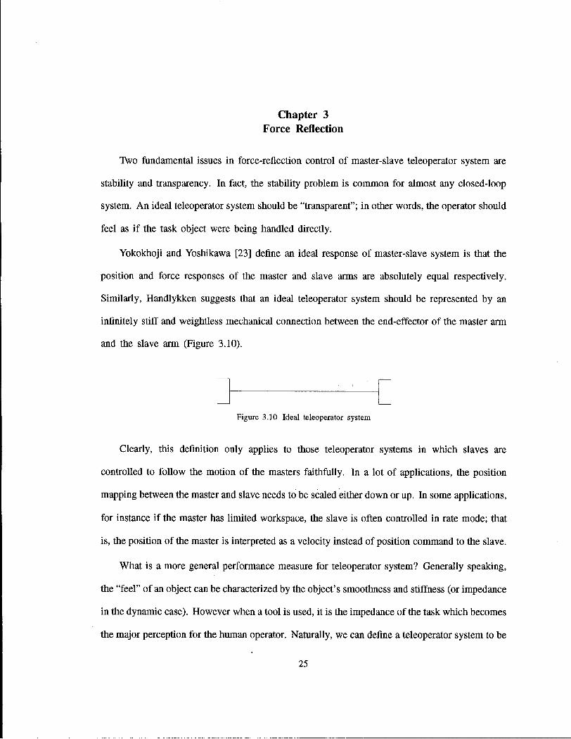
Similarly, Handlykken suggests that an ideal teleoperator system should be represented by an
infinitely stiff and weightless mechanical connection between the end-effector of the master arm
and the slave arm (Figure 3.10).
Figure 3.10 Ideal teleoperator system
Clearly, this definition only applies to those teleoperator systems i n which slaves are
controlled to follow the motion of the masters faithfully. In a lot of applications, the position
mapping between the master and slave needs to be scaled either down or up. In some applications,
for instance i f the master has limited workspace, the slave is often controlled i n rate mode; that
is, the position of the master is interpreted as a velocity instead of position command to the slave.
What is a more general performance measure for teleoperator system? Generally speaking,
the "feel" of an object can be characterized by the object's smoothness and stiffness (or impedance
i n the dynamic case). However when a tool is used, it is the impedance of the task which becomes
the major perception for the human operator. Naturally, we can define a teleoperator system to be
25

Chapter 3: Force Reflection 26
"transparent" i f the impedance "felt" by the operator, or i n other words transmitted to the operator
v ia the master-slave system, equals that of the task [22]. O f course, i n certain applications, such
as microsurgery dealing with human tissue, it would be desirable to have a scaled version of
the task impedance [32].
3.1 Network Representation of Teleoperator System
In network theory, an n-port is characterized by the relationship between effort, / (force,
voltage) and flow, v (velocity, current). For a linear time-invariant (LTI) lumped one port network,
this relationship is specified by its impedance, Z(s), according to
F(s) Z(s) =
V(s) (3.1)
where F(s) and V(s) are the Laplace transforms of / and v respectively. A L T I lumped two-port
network can be represented by its hybrid matrix which is defined as
= H(s) -V2
Vi F2
hn h\2
h2\ h22
Vi F2
(3.2)
one-port
H(S)
V2
H(S) H(S)
two-port
Figure 3.11 Network concepts

Chapter 3: Force Reflection 27
A suggested network representation of a master and slave telemanipulation system is a two-
port connected between two one-ports, the operator and the environment [15,19], see Figure 3.12.
v h
Operator +
H(S) +
Task
Z t o n e - P o r t two-port one-port
Figure 3.12 Network representation of teleoperator system
Using the hybrid matrix of the two-port and the task impedance
e ve
we can express the impedance "felt" by the operator as
Fh _ h\\{l + h22Ze) - h21h12Ze
(3.3)
Zt~vh
= 1 + h22Ze
(3.4)
Thus we have the following necessary and sufficient condition for transparency: / i n = h22 = 0
(3.5) hi2h2\ — — 1
Another useful concept in network theory is passivity. In the case of master-slave systems,
the condition for the total system to be stable is that the system itself must be passive if the
operator and environment can be regarded as passive system [23]. One useful tool in determining
passivity of a network is scattering theory .
Theorem [15]: A system is passive if and only if the norm of its scattering operator is less
than or equal to one, that is
1150)11 = sup \->[S*(jw)S(jw)} < 1 (3.6)

Chapter 3: Force Reflection 28
where * denotes complex conjugate transpose and A i ( . ) denotes the square root of the maximum
eigenvalue.
For a two-port network, the scattering operator can be related to its hybrid matrix as follows:
1 0 0 - 1
(H(s) -I)(H(s) + (3.7)
Anderson etc. [15] apply the scattering theory to the two-port time delayed communication
circuit which has the following hybrid matrix
H(s) 0 e~sT
-e-sT 0 (3.8)
where T is the time delay i n the communication line. It can be shown that the standard method of
communicating forces and velocity between the master and slave in a teleoperator system leads
to a nonpassive system for any time delay. This is the major cause of instabihty for position-
position architecture. Traditionally, a large amount of damping is added to the system to deal
with this problem. This i n turn degrades the system performance making it feel "sluggish". The
authors thus introduce an active control law to make the communication block identical to a
two-port lossless transmission line.
Passivity is a sufficient, but not necessary condition for stability. Quite often the two-port
master-slave subsystem is nonpassive while the entire system is stable. The passivity of the
master-slave system guarantee the stability when connected to any passive load. However this
guaranteed stability does not come without price. L a w n and Hannaford [16] reported a 50%
increase of task completion time with the above passivity based methods.
3.2 General Teleoperator Structure
In a conventional position control teleoperator system, either the contact force or the slave
position is fed back to the master to provide force reflection. The first is called direct force

Chapter 3: Force Reflection 29
feedback method, and the second is called coordinating force method. From the network point
of view, there are no specific reasons for not using the position and force information bilaterally.
The four-channel communication scheme gives us more freedom to achieve the desired hybrid
matrix which fulfill the requirement for transparency. Here, we adopt much of the formalism
presented in the earlier work by Lawrence [22]. A block diagram of a general teleoperator
structure is shown in Figure 3.13.
Figure 3.13 General teleoperator structure: After Lawrence, 1992

Chapter 3: Force Reflection 30
The symbols are defined as follow:
Z-m — MmS
Cm = Bm + Km J S
Zs = Mss
CS = BS + K./s (3.9)
Zh = the impedance of the operator's hand
= Mhs + Bh + Kh/s
Ze = the impedance of the environment - Mes + Be + Kjs
where Mm and Ms are the masses of the master and the slave respectively; Cm and Cs are the
transfer functions of the controllers; Assuming the operator's hand is a mass, damper and spring
system, Mh, Bh, and Kh are the mass, damper and spring coefficients; Me, Be, and Ke are
the mass, damper and spring coefficients of the task.
We can see the position-position and position-force structure are just two special cases of
this general structure.
The hybrid matrix of this two-port teleoperator system can be easily derived as
_ [Zm + Cm)(Zs + Cs) + C 1 C 4
D , C2(ZS + Cs) — C4
C3(Zm + Cm) + C\ ' ">21 =
h22 —
D 1 — C 2 C 3
D
where
D = Zs + Cs - C3C4 (3.11)

Chapter 3: Force Reflection 31
The transmitted impedance felt by the operator can be derived in terms of the block transfer
functions as
_ [{Zm + Cm)(Zs + Cs) + CiC4] + Ze(Zm + Cm + dC2)
1 (zs + cs- C3C4) + ze(i - c2c3) X i- }
Zt can be thought as the measure of transparency.
In linear control theory, stability of a closed-loop system can be checked by applying Nyquist
criterion to its loop transfer function LG = G{s)H(s). Thus LG can be regarded as the measure
of stability. Assuming the task is just a passive impedance and reorganizing the block diagram
of the general teleoperator system, we have the following for stability analysis.
C1~ C3Zh 2m + C m + Z .
1 Z s + C s
C1~ °3Zh Z m + C m + Z .
Figure 3.14 Closed-loop stability analysis
Assume that the individual master and slave control system are stable. C i , C2, C3 and C\ are
user specified transfer functions which should also be designed to be stable. In order to ensure
stability of the entire system, the Nyquist plot of the inner loop transfer function LG\ and the
outer loop transfer function LG2
C4{C\ - ZhC3)
1- r..\ (3.13)
LGi = (Zm + Cm + Zh)(Zs + Cs)
J^Q _ Ze(Zm + Cm + Zh(l - C2C3) + C\C2) {Zm + Cm + Zh)(Zs + Cs) - C4(ZhC-i - Ci)
can not encircle the critical point ( -1 + jO) on the Nyquist plot.

Chapter 3: Force Reflection
3.3 Force-reflecting Control
32
3.3.1 Coordinating Force
The position error between the desired and actual machine positions is usually proportional
to the contact force; therefore it is often used for force reflection instead of direct force feedback.
Other reasons for its popularity are: position sensing is much easier and less expensive to
implement than direct force measuring, and secondly coordinating force (position error) method
can be shown to be passive under position control. A block diagram of a position-position
structure is shown in Figure 3.15.
Operator
Figure 3.15 Position-position structure
If we choose Cm = Cs, the position-position structure can be reformulated using the network

Chapter 3: Force Reflection 33
concept, see Figure 3.16. It is known that any circuit network made up of strictly passive
• : 6
Figure 3.16 Network representation of position-position structure
components is itself passive, thus the system can not go unstable. The mechanical equivalent of
the above two-port teleoperator system is shown in Figure 3.17.
Operator
HAAAAM
Master-slave
—V\AAV— H H H
Task
K e
Me FVWWH--8-
Figure 3.17 Mechanical equivalence of position-position structure
It is quite often that the slave is controlled by the master under rate mode, that is the salve
velocity is proportional to the master position. For position servo, this is realized by adding an
integrator to the position forward channel, that is
Ci = Cs Bs +
Kvs Kvs (3.14)
where Kv is the velocity gain.

Chapter 3: Force Reflection 34
The coordinating force method can be easily be adapted to rate control. A block diagram
of such a rate-position structure is shown i n Figure 3.18. However, a " s t i f f controller (high
v d
KyS
Figure 3.18 Rate-position structure
position gain) can make the position error smaller than noise. Therefore it is not always possible
to implement this method in practice. For instance, the position gain is so high for hydraulic
mobile machines such as excavators and feller-bunchers that there is virtually no position error
for feedback considering the noise.
3.3.2 Force Feedback
It is wel l known that direct force feedback with position control can cause instabihty. Parker
[3] pointed out that stability problem is even more serious when direct force feedback is used

Chapter 3: Force Reflection
for rate control.
35
For general position control with direct force feedback, we have the following block transfer
functions (see Figure 3.19)
Kp
C2 = Kj (3-!5)
Cz = C4 = 0
where Kp, Kj are the position gain and force feedback gain respectively. The inner loop does
not appear i n this structure. The outer loop transfer function becomes
Z& (^Zm + Cm + Zh + ^C^j
2 (Zs + Cs){Zm + Cm + Zh)

Chapter 3: Force Reflection 36
The corresponding characteristic equation is
^ Ze (^Zm + Cm + Zfi + 7 ? ^ s )
(Zs + Cs)(Zm + Cm + Zk)
which can be rewritten as
T^-CsZe
^ (Zs + Cs + Ze)(Zm + Cm + Zh) ' ^
For stability analysis, it is equivalent to use the following loop transfer function:
LG ^r 3 jo, (Zs + Cs + Ze)(Zm + cm + zh)
For position control with direct force feedback, stability can be achieved by reducing the loop
gain J^J, but at the cost of reduced sensitivity.
For general rate control with direct force feedback, we have the following block transfer
functions
Kvs
C2 = K} (3-20)
C 3 = C 4 = 0
where Kv, Kf are the velocity and force feedback gain respectively. Compared with position
control, the difference is that the position gain Kp is replaced by Kvs. For stability analysis,
we have the following loop transfer function:
(Zs + Cs + Ze)(Zm + Cm + Zh)
It is wel l known from linear system theory, that the addition of pole at s = 0 to the transfer
function has an adverse effect on the system stability. In general, the result is to push the original
root loc i toward the right-half plane. On the Nyquist plot, adding a pole at s = 0 causes the
original Nyquist locus of G(jw)H(jw) to be rotated by - 9 0 degree making it easy for it to cross

Chapter 3: Force Reflection 37
the critical point (-1,0) on the complex plane. Therefore rate control with direct force feedback
tends to be unstable even without time-delay in the system.
Therefore it is not trivial to develop a scheme in which contact information is transmitted to
the operator while keeping the system stable under rate control. As we pointed out before, the
coordinating force method may be one option. However, as we discussed before, it might not be
possible in some applications where there are almost no position errors at all.
3.4 Transparency
3.4.1 Achieving Transparency Under Position Control
As Lawrence [22] pointed out, the position-position structure does not provide transparency,
nor does the position-force structure if the dynamics of the system can not be neglected.
It has been suggested by authors such as Salcudean [14], Lawrence [22] and Yokokohji [23]
that operator hand applied force should be fed forward to achieve transparency. Salcudean and
Wong applied this approach to a master-slave teleoperator system which consists of two identical
six DOF magnetically levitated wrist. Yokokohji and Yoshikawa reported similar work on a
single degree of freedom system.
It is clear that from the structure of the transmitted impedance
Zt = [(Zm + Cm)(Zs + Ca) + CiC 4] + Ze(Zm + Cm + CiC 2 )
(Zs + C S - C3C4) + Z e ( l - C2C3) (3.22)
that in order to make system fully transparent, i.e.,
Zt = Ze for any Ze (3.23)

Chapter 3: Force Reflection 38
the following conditions must be satisfied:
(Zm + Cm)(Zs + C.) + C 1 C 4 = 0
1 - c2c3 = 0
Zm + Cm + C\C2 = Zs + Cs — C 3 C 4
For position control, if we set
(3.24)
Ci — zs + Cs (3.25)
Solving the above system of equations, we have two possible solutions
C2 = 1
C 3 = 1
C 4 — —(Zm + Cm)
Zm ~\~ Cm
and C2
C3 = -
Zs + Cs
Zs -\- Cs
(3.26)
Zm ~\~ Cm
C4 = —{Zm + Cm)
where the second solution results in Z e = \, and therefore it should be eliminated.
The hybrid matrix for this "transparent" telemanipulator system can be derived as
(3.27)
H 0 1
- 1 0 (3.28)
Remarks:
1. It is interesting to note that the end point impedance of the system viewed from the slave
side equals:

Chapter 3: Force Reflection 39
which is the impedance of the human hand. In robotics control, the goal of impedance
control of a manipulator is to create a desired impedance at its end-effector. However, i n
practice, it is not very clear what the best impedance for the manipulator to contact its tasks
is. Experiences show human hands offer an adjustable impedance, which makes them ideal
for manipulating almost any object without encountering stability problem. Thus, from the
impedance control point of view, the above fully transparent teleoperator structure provides
a way to reconstruct the human impedance at the manipulator end-effector.
2. We have
Fh-Fe = (Zm + Cm){Vh - Ve) (3.30)
Fh - Fe = (Zs + Cs)(Ve - Vh)
the position error dynamics can be formed as
s(Zm + Cm +Zs + Cs)(xh-xe) = 0 (3.31)
where xh and xe are the positions of the master and slave respectively. Thus the slave tracks
the master position asymptotically. Therefore we indeed have realized the ideal weighdess
infinitely stiff bar asymptotically.
Apply ing Scattering Theory, we can compute the scattering matrix of the two-port as follows
1 0 0 - 1
{H(s)-I)(H(s) + i y 1 0 1 1 0
(3.32) S(s)
The norm of this scattering matrix is
\\S(jw)\\ = sup \*[S*{jw)S(jw)] = 1 (3.33)
Therefore, from the network point of view, this two-port is passive ("lossless" to be exact). Hence
when it is connected to any strictiy passive load, the system stability is ensured. Let ' s assume

Chapter 3: Force Reflection 40
the system is connected to two passive one-ports with impedance Zh (operator's hand) and Ze
(payload). The inner and outer loop transfer functions become
—(zm + Cm)(Zs + Cs — Zh) LGi
LG2 =
(Zm + Cm + Zh)(Zs + Cs) _ Ze(Zm + Cm + Zs -f Cs)
Zh{Zm + Cm + Zs + Cs)
(3.34)
The corresponding characteristic equations are
J^Q _|_ ̂ _ Zh{Zm + Cm + Zs -f Cs) _ Q (Zm + Cm + Zh)(Zs + Cs)
IQ2 -)- 1 - (^e + Zh)(Zm + Cm + Zs + Cs) _ Q (3.35)
Zh(Zm + Cm + Zs Cs)
A n y mass-damper-spring system is stable i f the mass, damping and spring coefficients are al l
positive. Thus, the inner loop and outer loop are stable; therefore, the entire system is stable.
The above teleoperator control strategy requires acceleration measurement. Furthermore, it
needs accurate knowledge of the mass of master and slave i n order to completely compensate for
their dynamics. This makes it difficult to implement i n practice. On the other hand, complete
transparency might not be desirable since an infinitely stiff and weightless'mechanical bar would
drift around i f it is not connected to a load and an operator. A s it is suggested by Salcudean and
Wong [21], a small centering force is desirable to "f ix" the. master and slave system to prevent
drifting. This, i n fact, can be interpreted as an intervenient impedance [23] added to the ideal
mechanical bar as shown i n Figure 3.20.
H W W \ H >
Figure 3.20 Intervenient impedance

Chapter 3: Force Reflection 41
Consequently, a small force is always needed to move the telemanipulator even without
payload. A s we w i l l see that the adding of intervenient impedance makes it unnecessary to
measure accelerations.
(3.36)
First let us add some damping and spring term to the master-slave subsystems
Zm = Mms + Bmc + Kmc/s
Zs = Mss + Bsc + Ksc/s
and set the block transfer function as
Ci = C s
C 2 = C 3 = 1 (3.37)
C4 = —Cm
Thus the corresponding transmitted impedance becomes
[(Zm + Cm)(Zs + Ca) + C1C4] + Ze{Zm + Cm + CiC 2 ) Z t (ZS + CS-C3C4) + Ze(l-C2C3) (3.38)
_ [ZmCs + ZsCm ~f ZmZs) -\~ Ze{Zm ~h C m + Cs) (Zs + Cs + Cm)
If we have identical master and slave subsystem, that is Zm = Zs, the transmitted impedance
becomes
Zt = Zm + Ze (3.39)
Thus the operator indeed feels the object's impedance and an intervenient impedance as we
expected.
The hybrid matrix for this telemanipulator structure becomes
H = Zm 1
. - 1 0 .
The end point impedance of the system viewed from the slave side equals:
(3.40)
Zend = -y = Zm + Zh (3.41)

Chapter 3: Force Reflection 42
which is the impedance of the human hand plus an intervenient impedance.
Since we have
Fh-Fe = ZmVh + Cm(Vh - ye) (3.42)
Fh - Fe = ZsVe + Cs(Ve - Vh)
In case of identical master and slave, that is Zm = Zs, the position error dynamics can be
formed as
s(Zm + Cm + Cs)(xh -xe) = 0 (3.43)
thus the slave tracks the master's position asymptotically. Therefore, we indeed have asymptoti
cally realized the ideal weightless infinitely stiff bar with an intervenient impedance.
The stability can be checked as before, starting from inner loop transfer function,
LG\ = -Cm{Cs - Zh) ^ 44) (Zm + Cm + Zh)(Zs + Cs)
The characteristic equation is
J^Q . | _ ] _ _ ( Z s + CS + Cm)(Zh + Zm) _ Q (Zm + CM + Zh)(Zs + CS)
(3.45)
Clearly the inner loop is stable.
For the outer loop
LQ2 Ze(Zm + Cm + Cs) ^ (Zs + Cs)(Zm + Cm + Zh) + Cm(Zh — Cs)
Again if we assume the master and slave subsystems are identical Zm = Zs, then
J^Q _|_]_— (Zfe + Zm + Ze)(Zm + Cm + Cs) _ Q (Zm + Zh)(Zs + Cs + Cm)
Therefore, the outer loop is stable.
(3.47)

Chapter 3: Force Reflection 43
However, the above stability analysis is based on the assumption that the master subsystem
is exactly the same as the slave subsystem, and the force feedback and feed-forward is accurate.
Salcudean [14] reported an error of only 5% i n the force feed forward could drive the system
unstable. In addition, as we discussed before, time delay is always a destabilizing factor i n the
system. The robust implementation of above scheme needs further study.
3.4.2 Achieving Transparency Under Rate Control
The position-force structure does not provide transparency nor does the rate-force structure.
Let 's have a look at what the operator feels i f the slave is controlled i n rate mode and direct
force feedback is used. The block transfer functions for rate-force control are
cx = ̂ - = Bs + ^ Kvs Kvs
c 3 = c 4 = 0
where Kv, Kj are the velocity gain and force feedback gain respectively.
The transmitted impedance becomes
_ (Zm + Cm)(Zs + Cs) + Ze \[Zm +Cm +
Zs + Cs + ze ^ Therefore it is difficult to say what the operator could feel from this transmitted impedance. For
large Ze , the impedance can be approximated as
Z t ^ Zm + Cm + ^p^1 (3.50) Rvs
For small Ze,
Z t ^ Zm + Cm (3.51)
A t these extremes, the operator could only feel some dynamics of the master-slave system; it has
nothing to do with the dynamics of the task.

Chapter 3: Force Reflection 44
A s we discussed before, for position control, the bilateral communication of force information
is important to achieve transparency. Here we can extend it to rate control.
In position control, a coordinating force is generated by the error between the desired and
actual slave position according to
Fco. — Cms(Xh — Xey (3.52)
where Cm = Bm + We can apply the same idea to rate control. However the coordinating
force under rate control takes the form of (see Figure 3.18)
Fco. — CmS [ -rr^ Xt (3.53)
Therefore it is natural to replace the block transfer function Cm i n the general teleoperator
structure with as shown i n Figure 3.21.
Operator
Figure 3.21 Achieving transparency under rate control

Chapter 3: Force Reflection 45
The transmitted impedance becomes
( Z ™ + fe) (Zs + Cs) + C l C 4 ] + Ze (Zm + + C1C2)
(Zs + C S - C3C4) + Ze(l - C2C3)
In order to achieve complete transparency, the following constraints must be satisfied:
(zm + ̂ yzs + cs) + c1c4 = o
1 - c 2 c 3 = 0
Cn Zm + ~rj V C\ C2 — Zs + Cs — C3C4 7̂ 0
For rate control, we set
C i Zs + Cs
K„s
After a few algebraic manipulations, we have the following solutions
C2 = Kvs
C 3 = 1
C4 = -Kvs \ Zm + Cn
and
C2
C3
C4
-K„s Zm +
Zs + Cs
1 Zs + Cs
— Iivs ( Zm -f
(3.54)
(3.55)
(3.56)
(3.57)
(3.58)
where the second solution results i n Ze = therefore it should be eliminated.
Unfortunately, the control law C 4 = -Kvs(^Zm + jf^) requires the measure of jerk which
is impossible i n practice. Instead, we can use the following simplified control law:
Kvs
C2 = Kvs
1 (3.59)
C
CA — —Cn

Chapter 3: Force Reflection 46
The corresponding impedance felt by the operator is as follows
(zmc. + Zfe + zmzs) + ze (zm + cs + f^)
(3. + Cs + fe) (3.60)
If we have identical master and slave subsystem, that i s " Z m = Zs, the transmitted impedance
becomes
Zt — Zm + Ze (3.61)
Thus we have the same impedance as for position control, which can be interpreted as the master
impedance plus the task impedance. The teleoperator system is transparent.
The hybrid matrix of the master-slave system can be computed as
H = L Kv
KyS 0
The transfer function between the master and slave velocities can be derived. Since
-Ve
hence
Vh Kvs
therefore the slave is indeed under rate control.
The stability can be checked as before, using the loop transfer functions,
_n (MM ZjA ^ m \ K v s Kvs)
LG2
(Zm + Jt; + zh)(Zs + Cs)
ze [zm + + C s ^
(zs + cs)(zm +cTs + zh)+cm(£-s-fe)
(3.62)
(3.63)
(3.64)
(3.65)
(3.66)

Chapter 3: Force Reflection 47
Under the assumption the master and slave are identical Zm — Zs, we have the following
characteristic equations,
(Zm + zh)(zs + cs + fc) LG1 + 1 = -. — ^ r *-L (3.67)
{Zm + j ^ + Zh)(Zs + Cs)
( Zm + + Cs ) (Zh + Zm + Ze) LG2 + l = ± - j-L —r— (3.68)
(Zm + Zh)[Zs + Cs + fe)
In order to guarantee stability, we must choose a control law such that the zeros of
Zm + %PL + C, = 0 (3.69) KyS
fall in the left half of the complex plane.
Compared with the position control, we have an additional feedback subsystem in this rate
control structure which is no longer guaranteed to be stable. In other words, we also have to make
the zeros of the following characteristic equations to be in the left half of the complex plane,
Zrn + ̂ L + Zh = 0 (3.70)
Zn + ^ - O - (3.71) Kvs
which are related to the master subsystem.
Equation 3.71 can be written as
KvMms3 + BmcKvs2 + (KvKmc + Bm)s + Km = 0 . (3.72)
It is known that in order for a polynomial equation to have no roots with positive real part, it
is necessary that
1. All the coefficients of the polynomial have the same sign
2. None of the coefficients vanishes.

Chapter 3: Force Reflection 48
Thus for stability reason, it is important to have Bmc ^ 0; otherwise, the system can not be stable.
During rate control, the position correspondence between the master and slave is lost.
Therefore the increase of spring force w i l l not be felt by the operator i f he can only feel the
impedance of the task. This can cause machine tip over (for instance, an excavator) or damage to
the tool. For these applications, it is more important to transmit the contact force to the operator
than to feel the task dynamics. However, as we discussed before, stability is still a problem.
3.4.3 Achieving Transparency Via Impedance Identification
A s we discussed before, it is not necessary to cancel the dynamics of the master-slave system
completely. Another interesting structure which could be used to make the system transparent is
v ia parameter identification [19]. Assume the task is merely a linear mass-spring-damper, that is
Ze = Mes + Be + - i s . (3.73)
A regression model can be formulated as
fe = [xe xe xe][Me Be Ke]T = yTe (3.74)
where ip = [xe xe xe]T and 9 = [Me Be Ke]T
On-line recursive least-squares estimation can be used to identify the task impedance param
eters. In addition, the resetting and forgetting factor technique can be employed to deal with a
changing environment. The estimated task impedance Ze then can be implemented i n the master
subsystem control as
Fh = ZmVh + ZeVh (3.75)
where Zm = Mms + Bmc +

Chapter 3: Force Reflection 49
Thus the impedance felt by the operator becomes
Zt = Zm + Ze (3.76)
which makes the system transparent.
A block diagram of the rate control with impedance identification scheme is shown in Figure
3.22.
Figure 3.22 Achieving transparency via parameter identification

Chapter 4 Stiffness Feedback
4.1 Principle
It has been shown that direct force feedback under rate control can easily introduce instabihty.
Parker [3] proposed a method in which the contact force is used to adjust the stiffness of the
joystick instead of being applied directiy to the operator's hand. A comparison of direct force
feedback and stiffness feedback is shown in Figure 4.23.
z„
Vd
( Rate-force Structure ) ( Rate-stiffness Structure)
Figure 4.23 Comparison of two rate control structures
The stiffness of the joystick can be adjusted according to
Km = Knom + feKrsgn(xh) (4.1)
Km is bounded by [Kmin, Kmax]
where Knom is a constant gain when there is no contact, KT is the ratio of stiffness and contact
force, see Figure 4.24.
50

Chapter 4: Stiffness Feedback 51
(X h > 0)
(xh < 0)
— : • f e
F_max '
Figure 4.24 Stiffness adjustment scheme
Within the linear area, the operator hand applied force equals to
fh = Mmxh + Bmxh + Kmxh
(4.2) = Mmxh + Bmxh + Knomxh + feKr\xh\
Thus, within this linear area, this stiffness adjustment scheme can be thought of as a special case
of direct force feedback whose feedback gain is linearly proportional to the master position. In
the case where the operator holds the master position constant, this gain is fixed; it is the same
as direct force feedback.
Clearly, this stiffness adjustment scheme does deliver the contact force information to the
operator to a certain extent. Numerical simulation and machine experiments show rate control
with stiffness adjustment can easily make the system stable. However, a stability analysis is
difficult to carry out for such a highly nonlinear system. The nonlinearity comes not only from
the stiffness adjusting mechanism but also from the master position deadband since a position
deadband is always needed for rate control. Stiffness feedback can be used for position control
as well .

Chapter 4: Stiffness Feedback 52
4.2 Stability
Rate control with stiffness adjustment makes the system highly nonlinear. Liapunov stability
analysis seems elusive for such a system [3]. However, careful examination of this control struc
ture reveals that the system can actually be divided into two separate second-order subsystems:
a master system with a varying spring and a slave system which tracks a desired path set by the
master (see Figure 4.25). We assume the operator's hand is modeled as a constant mass, damper
Master Subsystem Stable Slave Subsytem
Figure 4.25 Stiffness feedback control block diagram
and spring system. Since the slave subsystem is stable, one only needs to be concerned about
the stability of the master system (mass-damper-spring), that is
Mmxh + Bmxh + Km(fe)xh = fh, Bm > 0, Km(fe) > 0 (4.3)
where Km(fe) is only a function of the contact force fe and bounded as K m a x > Km(fe) >
It is helpful to study the following time-varying system which is quite similar to our problem
x + Bx + K(t)x = Q, B>0,K(t)>0 (4.4)
where for simplicity we assume unit mass.

Chapter 4: Stiffness Feedback 53
The behavior of a linear time^varying ( L T V ) system can be quite different from a L T I system.
We know that a mass-damper-spring system with constant positive coefficients x + Bx + Kx =
0 (B > 0, K > 0) is always asymptotically stable. However as we w i l l see, its time-varying
counterpart x + B(t)x + K(t)x = 0 (B(t) > 0, K(t) > 0) might be unstable. Special care
should be taken when dealing with L T V system. Before we start, let us have a taste of such a
difference. Consider the following second-order system
x + B(t)x + Kx = 0, B(t) > 0, K > 0 (4.5)
Instead of having a time-varying spring coefficient, the above system has a time-varying damping
coefficient. One might conclude that the equilibrium point (0, 0) is asymptotically stable i f the
damping coefficient B(t) remains larger than a strictiy positive constant, which implies constant
energy dissipation by the damper. Surprisingly this is not always true! Let 's have a look at
the following example:
x+ (2 + et)x + Kx = 0 (4.6)
with initial condition z(0) = 2, x(0) = - 1 , the above system has solution x(t) = 1 + e _ t
which goes to x(oo) = 1 instead. In fact, additional constraints are needed i n order to make
the equihbrium of above system asymptotic stable. It can be shown [Slotine and L i ] that one
sufficient condition is to satisfy the following
B(t) > a > 0
(4.7) B(t) <b<K
where a, b are positive numbers.
N o w we come back to our problem, that is a second-order system with time-varying spring
coefficient
x + Bx + K(t)x = 0, B > 0, K(t) > 0 (4.8)
Chapter 4: Stiffness Feedback 54
Without any additional constrains, it is easy to show that the system can be driven unstable by
changing K(t) even if it is bounded. For instance, a slightly damped mass-damper-spring system
goes unstable if we set the spring constant to a large value whenever the mass moves towards
the equihbrium point and a small value whenever the mass moves away from it. However, as
we will see later, the asymptotic stability can be guaranteed if certain conditions are satisfied.
First, we introduce some stability concepts from general LTV system theory.
Definition: A linear dynamical equation
E: X = A(t)X + D(t)U (4.9)
Y = C(t)X
is said to be totally stable, or T-stable for short, if and only if for any initial state and for any
bounded input, the output as well as all the state are bounded (refer to [33]).
It is clear total stability implies BIBO (bounded input/bounded output) stability. The
following theorem states that with some conditions on D(t) and C(t), uniformly asymptotic
stability implies total stability.
Theorem 4-1: Consider the dynamical equation
E : X = A(t)X + D(t)U (4.10)
Y = C(t)X
if the matrix D(t) and C(t) are bounded on ( - o o , oo ), then the uniformly asymptotic stability
of the zero state implies the system is T-stable (refer to [33]).
It is clear that for a LTI system, if its equUibrium point is asymptotically stable, then the
system is T-stable.
Next we will prove the following useful theorem, which provides a sufficient condition for
asymptotic stability for the master subsystem.

Chapter 4: Stiffness Feedback 55
Theorem 4-2: Consider the second-order time-varying mass-damper-spring system
x + Bx + K[t)x = 0, B > 0, K(t) > 0 (4.11)
Suppose K(t) is bounded by K m a x > K{t) > K m i n > 0 and
B2 - AKmax > 0 (4.12)
Under these conditions, the system is uniformly asymptotically stable. Further the trajectory on
phrase plan can cross the x axis at most once.
Remarks:
1. Since K{t) is bounded by K m a x > K(t) > K m i n > 0, condition B2 - 4Kmax > 0 implies
B2 - 4K(t) > 0 for all time. Thus; at each time instant, the system can be thought as a
overdamped, time-invariant, mass-damper-spring system.
2. This theorem makes no assumption on K(t).
Apply ing Theorem 4-1 and Theorem 4 -2 to the master-slave system, we have the following:
Corollary Consider the master subsystem
Mmxh + Bmxh + Km(fe)xh = fh, B> 0, Km(fe) > 0 (4.13)
where Km(fe) is only a function of the contact force fe and bounded by K m a x > Km(fe) >
Kmin > 0. Suppose
B2
m - 4MmKmax > 0 (4.14)
Under these conditions, the equihbrium point is uniformly asymptotically stable. Further this
system is T-stable; that is, any bounded input fh and arbitrary initial condition result i n bounded

Chapter 4: Stiffness Feedback
states, and bounded output i f the output takes the form of Y
bounded.
56
= C(t)[xh xh]T where C(t) is
It is interesting to note that the rate of change of Km(fe) does not affect the system asymptotic
stability as long as the its upper bound satisfies Bm - 4MmKmax > 0. In reality, the task
impedance can be strongly nonlinear, e.g. at the transition between contact and free space
motion. A quick contact with a hard surface could make the change of Km(fe) very rapid, even
nonsmooth. Addit ional nonlinearity comes from the master's position deadband. Nevertheless,
stiffness feedback under the condition Bm - 4MmKmax > 0 can guarantee asymptotic stability no
matter i f the payload is passive or active, linear or nonlinear; no matter i f there is a nonlinearity
such as the master position deadband; no matter i f there is a time delay i n the communication line.
Proof of Theorem 4-2
<Part 1> First, we show that starting from any arbitrary initial state on the phase plane, after
certain time, its trajectory must reach the x axis.
Assume the initial state is i n quadrant I V . Since in this quadrant the velocity is negative,
x w i l l decrease all the time. After a certain time, there are at most two possibilities as shown
i n Figure 4.26.

Chapter 4: Stiffness Feedback 57
dt
I I
X
\ 2 \ 1
I 3 v. \ E
Figure 4.26 Trajectory in phase plane
1. Trajectory reaches the x axis with x > 0.
2. Trajectory reaches the x axis with x < 0.
We only need consider the second case x < 0 and x = 0. It is clear the trajectory w i l l go into
quadrant 3. It can be treated later.
Assume that the initial state (x0, x0) is i n quadrant III. Since i n this quadrant, velocity is
still negative, x w i l l decrease. Secondly, since we have x = —Bx — K(t)x > Kmin\xo\ > 0 i n
this quadrant, x w i l l increase. Therefore, the trajectory reaches the x axis with x < 0 i n finite
time, as shown i n Figure 4.27.

Chapter 4: Stiffness Feedback 58
dX dt
I I
X
I I
Figure 4.27 Trajectory in phase plane
The same analysis applies to the other two quadrants due to symmetry.
<Part 2> Next we show that any trajectory starting from x axis (x — 0) goes to the origin
asymptotically without crossing the x axis.
We only need to consider the right half of the x axis due to symmetry.
Consider the time-invariant overdamped mass-damper-spring system
We have the following two observations:
(Observation 1): Any trajectory starting from (x = 0) goes to the origin asymptotically
without crossing the x axis.
x + Bx + Kx - 0, B > 0, K > 0 (4.15)
where
B - AK > 0 (4.16)

Chapter 4: Stiffness Feedback 59
Proof: The zero-input response of the system can be derived as follows:
x(t) = aeXlt + be*2*
x(t) = a A i e A l < + 6 A 2 e A ^
where A i , A 2 are the roots of the characteristic equation, that is
A i = VB2-4K)
a, b are two constants depending on initial state (x0, x0)
_ x0(Xi + B) + x0
(4.17)
(4.18)
b =
A i — A 2
x 0 ( A 2 + B) + xQ
(4.19)
A i — A 2
It is clear the system is asymptotically stable asi—>-oo, a ; , x - > 0 .
B y way of contradiction, we assume that the trajectory reaches the x axis at finite time
t = tc, that is
x(tc) = aeXlt° + beX2t° = 0 (4.20)
B y assumption we have xQ ^ 0 , x0 = 0, thus
= ( A i - A 2 ) t c
b A i + B (4.21)
a A 2 + B
Since we know A a - A 2 = ^B2 - AK > 0, the above equation implies
A 4- B Y—z > 1 or A i < A 2 (4.22) A 2 + n
which contradicts the fact that A i > A 2 . Therefore, it is not possible for any trajectory to reach
the x axis i n finite time.
(Observation 2): A t any state i n quadrant I V of the phase plane, the trajectory corresponding
to the system with higher stiffness has higher tangent.

Chapter 4: Stiffness Feedback 60
Proof: The tangent of a trajectory at state (x, x) for the time-invariant mass-damper-spring
system can be derived as
, „. dx x —Bx — Kx Tangent(K) = — = - = (4.23)
dx x x
Thus we have
Tangent(K + A) - Tangent(K) -Ax
> 0 (4.24)
i n quadrant I V .
From the above two observations, we can sketch the trajectories which correspond to the
systems with constant stiffness K m a x and i f m , - n respectively when starting from the same state P
on positive x axis, see Figure 4.28. The two trajectories can not intersect each either. Otherwise
it contradicts observation 2.
Qudrant four
_i i_
Figure 4.28 Trajectory in phase plane
N o w consider the second-order time-varying mass-damper-spring system
x + Bx + K(t)x = 0, B>0,K(t)>0 (4.25)

Chapter 4: Stiffness Feedback 61
which starts from the same initial state P. First, the trajectory of this time-variant system must
be bounded by curve 1 and curve 2; otherwise, it w i l l contradict Observation 2, see Figure
4.29. Second, since the velocity i n quadrant I V is negative, thus, any trajectory w i l l always
move towards to the left. Therefore, we conclude that as t —»• oo, the trajectory w i l l approach
the origin. Therefore, the system is globally asymptotically stable. This completes the proof
of Theorem 4-2.
Figure 4.29 Trajectory in phase plane

Chapter 5 System Overview
The focus of our research is to implement real-time, force reflecting, resolved motion control
for typical hydraulic mobile machines, an excavator and a feller-buncher. Previous work by
Parker [3] employed the same approach to control a three degree-of-freedom (DOF) log-loader.
Here, the results were extended to the manipulators with four and five D O F to further investigate
the application of resolved motion control (rate v.s. position) and force reflecting control (direct
force feedback v.s. stiffness feedback) for the control of the hydraulic mobile machines.
Master Slave
Wrist Machine
1 t Desired joint angles
I t A D / D A
Desired joint angles
A D / D A
1 t Desired joint angles 1 t DSP DSP DSP DSP DSP
^ 1
DSP
Hydraulic pressures and
Actual joint angles
Figure 5.30 Overall system configuration
The complete teleoperator system can be divided into two parts, the master subsystem and
the slave subsystem, as shown i n Figure 5.30. A six D O F magnetically levitated joystick as a
master is controlled by a local P I D controller with programmable center of compliance. The
62

Chapter 5: System Overview 63
Joystick position is interpreted as a command to generate a desired machine endpoint position.
Through an inverse kinematics transformation, the desired joint angles are computed and sent to
the hydraulic machine controller for set-point control. The hydraulic cylinder pressures and actual
joint angles are measured to calculate the endpoint force through inverse Jacobian transformation.
This force is reflected to the master side either directly applied to the operator's hand or used
to adjust the stiffness of the joystick.
5.1 Master — Maglev Joystick
The master plays a critical role in any master-slave teleoperator system. It serves as a
man-machine interface, therefore has great influence on the overall system performance.
Various kinds of joysticks can be used as the input devices. Passive joysticks are popular
due to the fact that they do not require actuators which makes them less expensive and less
complicated to build and maintain. After force-reflection was introduced i n teleoperation, great
efforts have been spent i n building ideal active joysticks which are capable of reproducing the
desired force to the operator's hand while providing enough D O F for operation. Most designs
use either hydraulic or electric servomotors. The nature of these actuators make it impossible
to overcome problems such as friction and backlash which greafly affect the performance of the
joystick.
The six D O F magnetically levitated joystick (Maglev Joystick) which is based on electrody-
namic actuation, originally designed for coarse-fine manipulation, proves to be ideal to be used
as a master for force-reflecting teleoperator system. Its novel design eliminate al l mechanical
linkages, and therefore friction and backlash.

Chapter 5: System Overview 64
5.1.1 System Configuration
A complete Maglev Joystick system [34] can be divided into four parts: a magnetically
levitated joystick which consists of a fixed "stator" and a moving "flotor", a signal conditioning
box, a digital controller with an A/D and D/A interface and a current driver, as shown in Figure
5.31. The Maglev Joystick Assembly is shown in Figure 5.32.
D / A current driver D / A current driver
digital controller
coils LED's
permanent magnets PSD's
flotor
A / D I
stator
signal conditioning box
Figure 5.31 Maglev Joystick system configuration

Chapter 5: System Overview 65
Flotor
LED Mounting Colums
PSD Mounts
Flotor Base
Support Post
Stator Base
Vertical Magnet Gap
Vertical Coil
Horizontal Coil
Horizontal Magnets
Figure 5.32 Maglev Joystick assembly3
5.1.2 Sensor and actuator
The internal position measuring of the Maglev Joystick is accomplished by optical sensors
which consist of light-emitting diodes ( L E D ) and position-sensing devices (PSD). Three L E D ' s
mounted at the center of the flotor project narrow, coplanar, radial light beams 120° apart
respectively onto the surfaces of the P S D ' s which are located at 120° intervals on the stator.
Typical resolutions for such system are approximately 1 \im for translation and 0.001° for rotation.
Actuation for the Maglev Joystick is based on an electrodynamic, moving coi l approach. Six
coils and six pairs of permanent magnets mounted on flotor and stator respectively comprise six
actuators which generate Lorentz forces to "f ly" the flotor. The joystick workspace is l imited by
the size of the magnetic gap. A large workspace requires large magnets and high electric currents
Joystick design by S. E. Salcudean, AutoCAD drawing by C. T. Chen

Chapter 5: System Overview 66
which in turn increase the overall size of the wrist and could cause heating problems. The UBC
Maglev Joystick has approximately + 5 mm translational motion and + 7° rotational motion from
the nominal center. Two coordinate systems are defined: the stator coordinate frame, attached
to the joystick stator, and the flotor coordinate frame, attached to the joystick flotor. The origin
of the flotor coordinate frame is located at the intersection of the projection axes of the LED's.
Due to the small motion range, the relation between the six coil currents and force-torque acting
on the rigid flotor can be approximately expressed as linear transformation
conditioned 6 x 6 constant matrix.
5.1.3 Control about the Remote Center of Compliance
The control of the Maglev Joystick can be treated as the control of a free rigid body in space.
By means of Remote Center of Compliance (RCC) control, we gain the ability to set the center
of compliance of the rigid body anywhere in space. In [34], the center of compliance is assumed
to be at the gravity center of the flotor. For the master-slave application, it is desirable to define
the center of compliance of the master to be at the center of the handle.
In addition to the stator and flotor coordinate frames, we need to define two extra ones on
the flotor: one called the tool frame which is at the remote center of compliance, the other called
the gravity center frame which is at the center of gravity. They have the same orientation as
the flotor frame, see Figure 5.33.
= MI (5.1)
where F f and Fr are the force and torque vector with respect to and expressed in the flotor
coordinate frame, I = [Ii 72 h h h hY * s a vector of six coils currents and M is a well-

Chapter 5: System Overview
Figure 5.33 Frame assignment
following symbols:
= the flotor's angular velocity in gravity frame
= flotor's inertia matrix i n gravity frame
= torque acting on the flotor with respect to gravity frame
= torque acting on the flotor with respect to flotor frame
= force acting on the flotor in flotor frame
= force acting on the flotor i n stator frame
We define the
GJ
GT
FT
Ff
f
GrT = coordinates of point T i n gravity frame
rT — coordinates of point T i n stator frame
FrG = coordinates of point G in flotor frame
Q = rotation matrix from stator frame to flotor frame
m = mass of the flotor
g = gravity constant

Chapter 5: System Overview
For any vector x = [xi x2 x3]T a skew-symmetric matrix xx is defined as follows:
0 -X3 x-i X3 0 -X\
- « 2 X\ 0
A X X =
The rigid body dynamics can be described by two differential equations
G,. = -Gj-l(G0JXGjG^+Gj-l GT
= l m
rT = ^-+g + QGoj(GcjXGrT) +
Q GrT
G J " 1 (Gu x G J Gu) - Q GrT
G J~l Gr
68
(5.4)
(5.5)
where the first is for rotation, and the second is for translation.
Using Euler quaternions, the rotation can be described by a vector p, which is defined by
P = [Po = [cos{4>l2) sin(4>l2)sT]T (5.6)
where s is the axis of rotation (||s|| = 1) and <j> is the angle of rotation.
The relations between the rotation matrix and Euler quaternions can be summarized as
follows:
Q = exV((f>sx) = I + 2(30p X + 2 / 3 X 2
(Q - QT)
2(1 + trQ)1'2
P2
0 + (3T(3 = 1 / 3 0 > 0
where trQ denotes the trace of Q.
Using the Euler quaternion representation and under the assumption of small angles and
small angular velocities, the rigid body dynamic equations can be simplified as
1 A ( 5 ' 8 )
rT = —f + g - G r T x G J - 1 G T = u2
m

Chapter 5: System Overview 69
Thus the dynamic equation can be easily transformed to decoupled second-order systems and
controlled by the following feedback law:
«i = Kp(Pd -•/?) - KvP
u2 = Kp(rd - rT) - KV rT
where KP,KV, KV and KV are diagonal gain matrixes.
The current-force mapping is defined with respect to the flotor coordinate. The following
transformation is performed to compute Fr and G f Ff = Q~1f*f
(5.10)
FT = F r a X F f + a T
Finally, the six coi l currents required can be calculated as
(5.11)
where M 1 is a constant matrix which can be precomputed.
Previously, due to lack of inertial parameters, a simple P ID control with gravity compensation
was used. Experiments show the performance of such a controller degrades when the center of
compliance is far away from the flotor center. Using parameter identification software developed
i n [35], the inertia matrix and the center of gravity of the joystick (with handle attached) were
identified. Remote center of compliance control has been successfully implemented.
5.2 Slave — Hydraulic Mobile Machines
Two typical hydraulic mobile machines have been used as slaves for the study o f force
reflecting teleoperator systems. The C A T 215 excavator is a four D O F manipulator mainly used
i n general construction industry while the C A T 325 feller-buncher with five D O F used i n the
forestry industry. The machine joint angles are sensed using resolvers and hydraulic pressures are
measured v ia pressure transduces. Both machines are outfitted with independent joint controllers
due to previous work by P. D . Lawrence, D . Chan and S. Bachman at U B C .

Chapter 5: System Overview 70
5.3 Computing System
Based on a V M E Bus structure, all the necessary processors, A / D and D / A boards can be
hosted i n one cage. The computing system configuration is shown i n Figure 5.34.
Figure 5.34 VME cage configuration
One S P A R C I E processor running the real-time multitasking operating system VxWorks and
one Skybolt board take care of the computations of joystick control, slave path planning and
force feedback. The Skybolt board which uses a 40 M H Z i860 processor is a specially designed
Math accelerator for Un ix hosts. N o w a new device driver makes it possible to directiy interface
with a VxWorks host to speed up VxWorks applications. The Skybolt, approximately 6 times as
fast as a S P A R C I E , performs all the real-time computations while the S P A R C I E handles timer
interrupts, collecting A / D data and sending D / A data. A shared memory block is defined at the
Skybolt side to communicate with VxWorks across the V M E Bus. The real-time control runs at
200 H Z . Another S P A R C running Unix and a T800 Transputer are included i n the same V M E
cage for the set-point control of hydraulic machines. The S P A R C / U n i x is the I/O host and the
Transputer performs the real-time computations.

Chapter 5: System Overview 71
The S P A R C / V x W o r k s board which is the host for the V M E cage is connected to Ethernet
allowing cross-development from a Unix host — Sun Workstation. This structure makes a user-
friendly environment for software development. Useful tools such as Stethoscope and Vxgdb can
be used for real-time data collection and program debugging.

Chapter 6 Machine Experiments
The master-slave multi-axes force-reflecting resolved motion control strategy was success
fully implemented on a CAT-215 excavator and a CAT-325 feller-buncher. Machine experiments
were carried out to investigate position versus rate control, stiffness versus force feedback control.
6.1 Endpoint Force Sensing
6.1.1 Modeling
Accurate force sensing is crucial for successful implementation of force feedback. In our
experiments, the hydraulic transducers were mounted i n the hoses close to the hydraulic pump.
The hydraulic pressures were used to compute the joint torques. For a discussion of other force
sensing methods, refer to [3] for details. Previously, Parker [3] used the Newton-Euler method
to derive a model for a log-loader which is three D O F manipulator.
During free motion, the manipulator's joint torques are caused by the following factors:
gravity of the links and the dynamic forces due to the machine motion. The dynamic equation
for a manipulator is:
T = D(q)q + C(q,q)q + g(q) (6.1)
where r = [ra r 2 ... r n ] T is the vector of generalized forces, q = [q\ qi ••• qn]T is the
vector of generalized coordinates of the system. When the manipulator contacts the environment,
the dynamic equation should be modified to include the effect of external force F, that is
Tt = D{q)q + C(q, q)q + g(q) + JT(q)F (6.2)
where J is the manipulator Jacobian.
72

Chapter 6: Machine Experiments 73
Thus in order to have an accurate measure of F, we need to know not only the joint torque
T, but also the dynamic model of the manipulator.
As discussed in [36], a key feature of rigid robot dynamics is its linearity in the parameters
although the dynamic equation itself is highly nonlinear. The dynamic equation of a manipulator
can be written in the following format, which is linear in the parameters
T = D(q)q + C(q, q)q + g(q) = Y(q, q, q )P (6.3)
where Y (q, q, q) is an nx r matrix of known functions of joint variables and P is an r-dimensional
vector of parameters which only depends on link mass, moments of inertia, etc. This property
of linearity in parameters makes it easy to identify the dynamic model through a parameter
estimation technique such as the Least-squares method.
It is possible to identify the complete model of a manipulator by using
r = D(q)q + C(q, q)q + g{q) = Y(q, q, q )P (6.4)
The joint velocities q and accelerations q are required to obtain P. However, in practice, q is
not available even if q can be measured, and digital differentiation of q is noisy. Secondly, even
for a two link manipulator, the vector of parameters P contains nine components (see Spong
[36]). The complete model of a four or five DOF manipulator would be much more complicated.
Therefore, in our experiments, only the static case is modeled, that is
r = g(q) (6.5)
and the contact force at end-effector is approximated by
F^(jT(q))-\rt-g(q)) (6.6)

Chapter 6: Machine Experiments 74
where rt is a vector of the joint torques computed from the hydraulic pressures, g(q) can be
obtained from the measured joint angles and the l ink parameters.
Thanks to the powerful symbolic computation package Maple, a computer program was
written to derive the static model of manipulator automatically using the Euler-Lagrangian
formulation. The procedure is straightforward: first, the forward kinematics is performed to locate
the gravity center of each link, then the potential energy of the system is computed symbolically.
Finally, the joint torques are derived by differentiating the potential energy, according to
(6.7)
There are several advantages of using a computer program to derive the manipulator model:
1. Speed: the Maple program can generate a dynamic model within 2-3 seconds.
2. Correctness: once the program is running, by changing the manipulator l ink parameters, such
as l ink distance, length and twist, we can easily get the result for manipulators with different
configurations, and guarantee its correctness.
3. Efficiency: the simple procedure can be applied to manipulators with any number of degrees
of freedom, and is easy to debug. This can save tedious algebraic manipulation when dealing
with robot with high D O F . Besides, Maple has many easy-to-use functions to either simplify
the results or to shape them to the format you like. These all can be done within a few
seconds.
We have also successfully derived the manipulator Jacobian for the excavator and the feller-
buncher symbolically using the Maple program. This is very helpful i n real-time applications.

Chapter 6: Machine Experiments 75
Static Model of the Excavator
" 0 0 0 0 0 0 "
T = Y(q, q, q)P = C*234 C*234
5 234 5 234
C23
C23
^23 <5"23
c2
0 s2
0 .C234 5 234 0 0 0 0 .
[n r 2 r 3 T4]t, P = [Pi Pi Pz PA P5 Pef, £234 = sin (02
(6.8)
Static Model of the Feller-buncher
" 0 0 0 0 0 0 0 " 0234(75 C234 5234 C*23 523 c2 s2
q)P = C234C5 C*234 5234 C 2 3 523 0 0 p C234C5 C*234 5234 0 0 0 0
. — 523455 0 0 0 0 0 0 .
(6.9)
where r = [n r 2 r 3 r 4 r 5 ] T , P = [P a P 2 P3 PA PS Pe Pjf, S23A = sin (62 + 93 + 94) etc.

Chapter 6: Machine Experiments 76
Jacobian of the Excavator
The nonzero elements of the Jacobian are as follows:
J[0][0] = d2
J[2][0] = — 0-\C 234 ~ a3C23 ~ O2C2
j \ m = 1.0
J[0][1] = — a4>5,234 — 0-3S23 ~ &2S2
J[l][l] = a4C234 + a3C23 + ^ 2 ^ 2
J[5][l] = 1.0
J[0][2] = — G'4'5'234 — a3*523
J[l][2] = a4C234 + A 3 C 2 3
J[5][2] = 1.0
7[0][3] = — a4'5'234
J[l][3] = a 4 C 2 3 4
J[5][3] = 1.0
(6.10)
where J is the manipulator's Jacobian with respect to frame Ci , S234 = sin (0 2 + 03 + # 4 )
etc.

Chapter 6: Machine Experiments
Jacobian of the Feller-buncher
The nonzero elements of the Jacobian are as follows:
77
J[0] [0] = — CI5S5
J[2] [0] — — a\ — 0.5a5C234-5 — 0.5a5C2345 — 0.2^2 + ^5^234 ~ a4C<234 —
J[4] [0] = 1.0
J[0] [1] = — a2S2 — CI3S23 — a4-5234 — d5C234 — 0.5a55234_5 — 0.50552345
J[l] [1] = 0 .5a 5 C 2 34_5 + 0.5a5C2345 + a 2 C 2 - d5S234 + «4C*234 + a3C23
J[5] [1] = 1.0
J[0] [2] = — ^ 3 ^ 2 3 — a4<S234 — dsC234 — 0.505^234-5 — 0.505̂ 2345
J[l] [2] - 0.5a5C234_5 + 0.5a5C2345 — ^5^234 + aiC234 + 03 *̂23
J[5] [2] 1.0
J[0] [3] = — 04^234 — d^C234 ~ 0.5a55234-5 — 0.5(1552345
J[l] [3] — 0.5a5C234_5 + 0-5a5C2345 — ^5234 + a4p234
J[5] [3] = 1.0
J[0] [4) — 0.5as5234-5 - 0.5O5 52345
J[l] [4] - -0 .5a 5C 234-5 + 0.5a5C2345
J[2] [4] - a 5 C 5
J[3] [4] - -5234
J[4] [4] = C*234
where J is the manipulator's Jacobian with respect to frame C i , 5234 =
sin (02 + 03 + 04), 5234-5 = sin (02 + 03 + 04 - 05) etc.

Chapter 6: Machine Experiments 78
6.1.2 Torque Computations
The hydraulic cylinder force can be computed from the hydraulic pressures and the cylinder
geometry:
Fcyl = PinAin ~ Pout-^-out (6.12)
where P,- n , Pout are the pressures at the piston head side and rod side respectively, A , - n , Aout
are the areas at the piston head side and rod side.
L i n k Name Head Area i n (in2) R o d Area i n (in2)
B o o m 31.80 19.92
Stick 23.75 14.13
Bucket 15.90 9.96
Table 6.3 Piston geometry of the excavator
L i n k Name Head Diameter i n (mm) R o d Diameter in (mm)
B o o m 120.00 85.00
Stick 150.00 105.00
Tdt 150.00 105.00
Head 152.40 63.50
Table 6.4 Piston geometry of the feller-buncher
Referring to the excavator and feller-buncher schematics Figure 1.3 and Figure 1.5, there are
only two types of mechanical linkage on these machines: two-bar linkage and four-bar linkage,
see below:

Chapter 6: Machine Experiments 79
Figure 6.35 Two-bar mechanical linkage
Figure 6.36 Four-bar mechanical linkage
Joint torques can easily be derived for a two-bar linkage as the following:
, , , „ , a&lsin B\ r = \Fcyl\ . 1 n (6.13)
where Fcyl is the hydrauhc cylinder force, B is the joint angle, a and b are the linkage lengths.
For the torque computation of a four-bar linkage, refer to [37] for detail.

Chapter 6: Machine Experiments
Boom
Two-bar Linkage
Stick
Two-bar Linkage
Bucket
Four-bar Linkage
a = 1999.8 (mm) b = 624.0 (mm)
a = 720.2 (mm) b = 2443.6 (mm)
rl = 324.9 (mm), r2= 404.9 (mm) r3 = 484.9 (mm), r4 = 548.6 (mm) 7 = 0.0468407 (rad) a = 0.3469905 (rad) L = 1602.7 (mm)
Table 6.5 Joint linkage geometry of the excavator
Boom
Two-bar Linkage
Stick
Two-bar Linkage
Tilt
Four-bar Linkage
Head
Two-bar Linkage
a = 2281.6 (mm) b = 911.2(mm)
a - 901.2 (mm) b = 2339 (mm)
rl = 481.3 (mm) r2 = 563.7 (mm) r3 = 640 (mm) r4 = 685 (mm) 7 = 0.0728 (rad) a = 0.1831 (rad) L = 2316.3 (mm)
a = 634.0 (mm) b = 588.0 (mm)
Table 6.6 Joint Linkage geometry of the feller-buncher

Chapter 6: Machine Experiments 81
6.1.3 Recursive Least-squares Link Parameter Estimation
There are several reasons for using a recursive estimation method. First, it is l ikely that some
experimental data are corrupted due to factors such as temporary sensor or transmitter failure, etc.
Since the number of observations is always limited, these outliers can have a strong effect on the
estimated parameters. Thus it is important to evaluate the estimated parameter over the full range
of observation so that the residuals can be examined to find out any "bad data" which is responsible
for large residual values. In our case, these outiiers can be eliminated, and the estimation
procedure repeated. Secondly, from the plots, we can get information such as convergence. Wi th
this information, we can get some idea as to what degree of accuracy the estimated parameters
have. In the case of nonconvergence, we can reexamine the whole procedure including the way
the experiments were carried out, find the cause, then take appropriate measures. During the
experiments, the hydraulic machines were commanded to move slowly from one configuration
to another randomly while the joint angles and hydraulic pressures were recorded. Then, these
data were subsampled for off-line estimation. The initial parameters and the covariance matrix
were computed from the first 50 sets of data. The recursive Least-squares estimation results for
the excavator and the feller-buncher are shown i n Figure 6.37 — Figure 6.44 i n which we call
each set of data one "sample".

Chapter 6: Machine Experiments
X 1 0
-r- 1.5
§ 0 . 5 h
- 0 . 5
Least -squares Parameter Identification
sample 2 0 0 2 5 0
x 1 0 Least -squares Parameter Identification
2 5 0 sample
Figure 6.37 Excavator link parameter identification

Chapter 6: Machine Experiments
Figure 6.38 Excavator link parameter identification

Chapter 6: Machine Experiments
Figure 6.39 Excavator link parameter identification

Chapter 6: Machine Experiments
O 50 100 150 200 250 sample
Figure 6.40 Excavator link parameter identification

Chapter 6: Machine Experiments
x 10 L e a s t - s q u a r e s P a r a m e t e r Iden t i f i ca t ion
E to
2 0 0 s a m p l e
4 0 0
x 1 0 L e a s t - s q u a r e s P a r a m e t e r Iden t i f i ca t ion
100 1 5 0 2 0 0 s a m p l e
2 5 0 3 0 0 3 5 0 4 0 0
Figure 6.41 Feller-buncher link parameter identification

Chapter 6: Machine Experiments
x 1 0 L e a s t - s q u a r e s P a r a m e t e r Iden t i f i ca t ion
2 0 0 s a m p l e
4 0 0
x 1 0
1.8r
1 .6r
1 .4r
- 1 . 2
L e a s t - s q u a r e s P a r a m e t e r Iden t i f i ca t ion
CD ^ 5 11 E 0.8|( I
0.6H
0.4H
0.2H-
2 0 0 s a m p l e
2 5 0 3 5 0 4 0 0
Figure 6.42 Feller-buncher link parameter identification

Chapter 6: Machine Experiments
L e a s t - s q u a r e s P a r a m e t e r Iden t i f i ca t ion 1 1
J L _
J
I _
•
O 5 0 1 0 0 1 5 0 2 0 0 2 5 0 3 0 0 3 5 0 4 0 0 s a m p l e
Figure 6.43 Feller-buncher link parameter identification

Chapter 6: Machine Experiments 89
Figure 6.44 Feller-buncher link parameter identification

Chapter 6: Machine Experiments 90
6.2 Excavator Experiments
The master-slaver force reflecting resolved motion control was first implemented on a four
D O F manipulator — C A T 215 excavator. The machine was operated remotely from a nearby
lab. The first set of experiments focused on resolved motion control — position versus rate.
Hands-on experiences confirmed the results reported by K i m [8] that for a slow manipulator such
as a hydraulic excavator, rate control is preferable. The mismatch of the fast joystick and the
slow excavator could cause oscillation under position control, on the other hand, an operator can
easily achieve a smooth operation when the machine is under rate control. Whi le position control
is important i n some delicate operations such as peg-in-hole or microsurgery etc., the application
of such control to hydraulic machines is not suitable at least from the operator's point of view.
The second set of experiments were carried out to test different force reflection schemes, namely
stiffness versus direct force feedback.
The following gains were selected for the joystick control during the experiments (see Figure
4.24):
A x i s K p max K p nom K p min K d Deadband
X 4.0 0.6 0.3 0.06 1.5
Y 4.0 0.6 0.3 0.06 1.5
Z 4.0 0.6 0.3 0.06 1.5
X Rotation 0.1 0.06 0.01 0.03 2000.0
Y Rotation 0.1 0.06 0.01 0.03 50.0
Z Rotation 0.1 0.06 0.01 0.03 2000.0
Table 6.7 Gain selections for the excavator experiments
In the above table, Kp(max) i s the maximum stiffness value, Kp(nom) is the nominal stiffness
value, Kp(min) is the minimum stiffness value (units: N / m m for translation and 100 Nm/rad for

Chapter 6: Machine Experiments 91
rotation); K d is the damping factor (units: N/mm/s for translation and 100 Nm/rad/s for rotation);
The units for the joystick deadband are m m for translation and O.OOOlrad for rotation.
The contact force for feedback is saturated by the following values:
A x i s X Y Z X Rotation X Rotation X Rotation
F_max 50 ( K N ) 50 ( K N ) 50 (KN) 40 (KNm) 40 ( K N m ) 40 ( K N m )
Table 6.8 Maximum feedback force for the excavator experiments
6.2.1 Resolved Motion Control
The machine was under rate control and operated remotely to achieve straight line motions.
Figure 6.45 and Figure 6.46 show the bucket was commanded to go straightly up and down
while keeping the bucket angle and radial displacement constant. Figure 6.47 and Figure 6.48
show the bucket was directed to come straightly out from and i n towards the cabin while keeping
the bucket angle and height constant. The joystick deadband is 1.5 mm. It is clear from these
plots that the motion accuracy is high due to the fact inverse kinematics instead of Jacobian
transformations were used and the joint angles of the excavator were under closed-loop control.

Chapter 6: Machine Experiments 92
E x c a v a t o r C o n t r o l ( r e s o l v e d m o t i o n )
t i" >
1 1 1
r
^
1 i a __
1
x 1
i i
i
; y ! T
'•
i i
i
1 . 2 1 i i J I 1_
O 0 . 5 1 1.5 2 2 . 5 T i m e ( s e c o n d s )
Figure 6.45 Excavator resolved motion control: bucket straight up

Chapter 6: Machine Experiments 93
E x c a v a t o r C o n t r o l ( r e s o l v e d m o t i o n ) T
0 . 5 1 .5 T i m e ( s e c o n d s )
2 . 5
E x c a v a t o r C o n t r o l ( r e s o l v e d m o t i o n ) 7 1 1 1
J 1 i 1 1 1 O 0 . 5 1 1.5 2 2 . 5 3
T i m e ( s e c o n d s )
Figure 6.46 Excavator resolved motion control: bucket straight down

Chapter 6: Machine Experiments 94
Figure 6.47 Excavator resolved motion control: bucket straight out

Chapter 6: Machine Experiments 95
E x c a v a t o r C o n t r o l ( r e s o l v e d m o t i o n )
1 z
X \
- t
; y
i i
T
_L L J
i
i
j
1
i i
;
i
r T
X l
<•
O 0 . 5 1 1.5 2 2 . 5 3 T i m e ( s e c o n d s )
E x c a v a t o r C o n t r o l ( r e s o l v e d m o t i o n )
I
L
\
r
— i ~
~ ~ " T
L
L
' t h e t a 1
z
r
\ I I I
H - 4 0
3, £ 0 •33 J=
a>
- 2 0 i f
H o 0.5
1.5 T i m e ( s e c o n d s )
2 . 5
Figure 6.48 Excavator resolved motion control: bucket straight in

Chapter 6: Machine Experiments 96
6.2.2 Applying a Desired Force
This experiment is to test the ability of an operator to apply a desired force to the environment
v ia our force reflection master-slave teleoperator system. The operator sat i n the lab and remotely
commanded the excavator to contact the ground. A t the beginning, he was allowed to look at the
force display on the screen to relate the contact force to the kinesthetic feel at his hand. Then the
operator was asked to apply a desired force to the ground depending solely on the information
from the joystick. The operator's hand applied forces were measured using JR-3 force sensor.
Two force reflection methods were tested — stiffness and direct force feedback. Results are
shown i n Figure 6.47 and Figure 6.48 respectively. Both methods achieved reasonably good
results i n terms of controlling the endpoint force. However, direct force feedback method is only
possible when the amount of force feedback is severely restricted. Otherwise, stability problems
can arise. In stiffness control (Figure 6.47), the operator's hand applied force is proportional to
the wrist displacement along corresponding z axis. In direct force feedback (Figure 6.48) while
the operator applied - 4 . 5 Newton force to the wrist to counterbalance the feedback force there
is almost no wrist displacement i n z axis.

Chapter 6: Machine Experiments 97
E x c a v a t o r C o n t r o l ( s t i f fness c o n t r o l )
i i i X I 1 1
, ^ 1 J I > 1 "1
y ^ l _ ^ J
Fh_z f k - -
1
1
* -1
-o -2 .22 •Q. Q-<C # -3 E ,
-4
0 . 5 1.5 T i m e ( s e c o n d s )
2 . 5
x 1 0 E x c a v a t o r C o n t r o l ( s t i f fness c o n t r o l ) T " T"
3 . 5 h
I
i t a r ge t
! ^
u l i i i i V i i i i i
1 1 1 1 1 1 1 1 1 1
1
L
r
— 2 . 5
* 2
CO
" 1.5
0 .5 r -
0 . 5 1 .5 T i m e ( s e c o n d s )
2 . 5
Figure 6.49 Excavator stiffness control: applying a desired force

Chapter 6: Machine Experiments 98
E x c a v a t o r C o n t r o l ( fo rce c o n t r o l )
T i m e ( s e c o n d s )
E x c a v a t o r C o n t r o l ( fo rce c o n t r o l )
8
% 2
« o " 1.5
t \ \ I \ I I I I I I I I I I
A | t a r ge t 1
1
l i l * i i
I I I l I
l I I I l I I I l l l i - l i i
L
• i
i i —
1 ,
<<
+ !
1 \
1 - — —
O 0 . 5 1 1 .5 2 2 . 5 3 T i m e ( s e c o n d s )
Figure 6.50 Excavator force control: applying a desired force

Chapter 6: Machine Experiments 99
6.3 Feller-buncher Experiments
The master-slaver force reflecting resolved motion control was also implemented on a five
D O F manipulator — C A T 325 feller-buncher. The master Maglev Joystick was mounted i n the
cabin during the experiments. F ie ld tests such as tree-cutting were also carried out. Experiments
show that while the sound of the engine and the motion of the machine do provide the operator
with information to detect potential machine tip over, the most effective way is v ia force reflection
which automatically pushes the joystick back into its position deadband. Similar to the excavator
experiments, position control was found to be unsuitable for the control of the feller-buncher.
Direct force feedback is possible only i f the amount of feedback is severely limited.
The following gains were selected for the joystick control during the experiments (see Figure
4.24):
A x i s K p max K p nom K p min K d Deadband
X 8.0 4.0 3.00 0.06 1.5
Y 4.0 3.0 2.00 0.06 1.5
Z 9.0 4.0 3.00 0.06 1.5
X Rotation 0.8 0.45 0.30 0.04 350.0
Y Rotation 0.8 0.45 0.30 0.04 350.0
Z Rotation 0.26 0.25 0.24 0.04 2000.0
Table 6.9 Gain selections for the feller-buncher experiments
In the above table, Kp(max) is the maximum stiffness value, Kp(nom) is the nominal stiffness
value, Kp(min) is the minimum stiffness value (units: N / m m for translation and 100 Nm/rad for
rotation); K d is the damping factor (units: N/mm/s for translation and 100 Nm/rad/s for rotation);
The units for the joystick deadband are m m for translation and O.OOOlrad for rotation.

Chapter 6: Machine Experiments
The contact force for feedback is saturated by the following values:
100
A x i s X Y Z X Rotation X Rotation X Rotation
F_max 30 ( K N ) 30 (KN) 30 ( K N ) 40 (KNm) 40 ( K N m ) 40 (KNm)
Table 6.10 Maximum feedback force for the feller-buncher experiments
Hydraulic mobile machines such as excavators and feller-bunchers often operate i n harsh
environments. Bumpy road conditions can cause undesired motion of the joystick. Thus it is
desirable to have a stiff joystick. On the other hand, an operator may get tired from manipulating
a stiff joystick during normal operation. A l so , a stiff joystick could easily cause heating problem.
Another problem often encountered when using multi-degree joysticks is coupling between
joystick axes. A motion i n one direction could easily cause an unexpected motion i n another.
In order to solve these problems, a detent scheme was implemented i n the digital P I D
controller, as shown i n Figure 6.51.
i
LL
••-"~""[
Deadband
X
Figure 6.51 Detent implementation

Chapter 6: Machine Experiments 101
X
Figure 6.52 Conventional position control
For conventional position control (see Figure 6.52), the restoring force is a linear function
of the position error. The bigger the position error, the higher the restoring force. In detent
implementation, there are two slopes. Within the joystick position deadband, it is the same as the
single slope approach. Outside this band, it has another slope which is lower than the first one.
At the edge of the band, there is fixed amount of force drop. Clearly with this detent scheme, we
can achieve high stiffness within the position deadband (desirable when machine travels) without
having a high restoring force during normal operation which is outside the deadband. An operator
can feel a "notch" when the joystick crosses the edge of the deadband. This is a good hint to the
operator as to which area he is working in. As a result, decoupling between axes is achieved to
a certain degree. Experiments show reduced restoring force outside the deadband makes normal
operation easy which in turn reduces undesired motion in other axes.

Chapter 6: Machine Experiments 102
X Y Z X Rotation Y Rotation Z Rotation
Force Drop 2.00 (N) 2.00 (N) 2.00 (N) 0.8 ( N M ) 0.8 ( N M ) 0 ( N M )
K p 4.0 3.0 4.0 0.45 0.45 0.25
K p l 0.3 0.3 0.4 0.03 0.03 0.25
Table 6.11 Detent parameters for the feller-buncher experiments
In the above table, the units for stiffness are N / m m for translation and 100 Nm/rad for rotation
6.3.1 Desired Force Tracking
This experiment aimed to investigate the difference between teleoperation with and without
force reflection i n controlling the end point force. During the experiment, the operator controlled
the machine inside the cabin. The contact force was collected and displayed on a computer screen
to provide additional guide to the operator. First, the operator commanded the machine under
stiffness feedback to contact a solid rock and tried to follow a desired force trajectory displayed
to h i m as a graph on the computer screen shown i n Figure 6.53. Next, the operator repeated the
same experiment except that there was no force reflection present, see Figure 6.54. Experiments
indicate that it is very hard to track a desired force trajectory without the use of force reflection.
The results clearly demonstrate that the addition of force reflection to the teleoperator system
greatly improves the ability of the operator to control the endpoint force.

Chapter 6: Machine Experiments
F e l l e r - b u n c h e r C o n t r o l ( s t i f fness c o n t r o l )
-2
1 5 2 0 2 5 T i m e ( s e c o n d s )
3 0 3 5 4 0
x 1 0 F e l l e r - b u n c h e r C o n t r o l ( s t i f fness c o n t r o l ) T
S 3 h
° 2 r
|
8 I -K
F z
O h
t a r ge t ! r | i «
1 0 1 5 2 0 2 5 T i m e ( s e c o n d s )
3 0 3 5 4 0
Figure 6.53 Feller-buncher stiffness control: force tracking

Chapter 6: Machine Experiments 104
F e l l e r - b u n c h e r C o n t r o l (wi thou t f o r c e - r e f l e c t i o n )
2 0 2 5 T i m e ( s e c o n d s )
4 0
x 10 F e l l e r - b u n c h e r C o n t r o l (wi thou t f o r c e - r e f l e c t i o n )
o O
\ ! 1
n
I "
4 I
t a r ge t
10 1 5
i *
f f .
'11
r-
• 11
:T""
2 0
J
2 5
V
30
\
35 4 0
Figure 6.54 Feller-buncher control without force-reflection: force tracking

Chapter 6: Machine Experiments
6.3.2 Complete Tree Cutting Process
105
Quantitative data for complete tree cutting process is shown i n Figure 6.55. The operator
first commanded the felling-head of the feller-buncher to approach a tree. The endpoint force
increased rapidly after contact with the tree was made. Through the change of stiffness of the
joystick, the operator could feel this contact kinesthetically, see the hand applied force (which is
approximated by the centering force of the joystick) i n Figure 6.55. Whi le this was happening,
the rotating saw started cutting the tree, and the grab arm on the felling-head closed and grabbed
it. The cut tree was then laid to the side i n bunches.

Chapter 6: Machine Experiments
x 10 F e l l e r - b u n c h e r C o n t r o l ( s t i f fness c o n t r o l ) T
3 . Q_ £ Oh ZD CO CO CD O .
-2h-
- V -
I Grab arm . starts dosiri!
o O
- 4 h
I « 1 1 I
Grab arm finishes s dosind
/i
1A n A
v/y\ .'1' - \ - - - H
130 131 1 3 2 1 3 3 1 3 4 1 3 5 1 3 6 T i m e ( s e c o n d s )
1 3 7 1 3 8 1 3 9
Figure 6.55 Feller-buncher stiffness control: tree cutting process

Chapter 6: Machine Experiments
6.3.3 Practical Issues
107
For simplicity, only the static models of the manipulators were used for force computation.
During free motion, the joint torques caused by the manipulators dynamics can introduce big
computed-force error. Figure 6.56 — Figure 6.58 show the joint step responses of the feller-
buncher , from which we can see that huge hydraulic pressures oscillations during free motion.
Clearly, the static model of the manipulator without considering the actuator dynamics is not
enough. One option is to completely model the manipulator dynamics. This might be hard in
practice as wel l because there is large amount of friction present i n the system. Other methods,
such as direct force sensing v ia load cells, as suggested i n [3], were not pursued due to the lack
of time. Although the force resolution is not ideal, the experiments show that force reflection
did help the operator to control the endpoint force effectively.

Chapter 6: Machine Experiments
Figure 6.56 Feller-buncher step response: boom

Chapter 6: Machine Experiments 109
Figure 6.57 Feller-buncher step response: stick

Chapter 6: Machine Experiments
time(sac)
Figure 6.58 Feller-buncher step response: tilt

Chapter 7 Conclusions
Issues concerning the design and implementation of master-slave force-reflecting resolved
motion control for hydraulic mobile machines are addressed i n this thesis. A six D O F mag
netically levitated joystick is employed as the teleoperator master which proves ideal for the
application of force reflection. Machine experiments show rate control is preferable to position
control for slow response slave manipulators such as excavators and feller-bunchers. Gravity
torque cancellation for end-effector force sensing is effective, but not complete. The dynamic
model of the manipulator is needed i n order to eliminate the dynamic torque, especially dur
ing free motion. Whi le direct force feedback under rate control can easily introduce instability,
stiffness feedback provides a promising way i n controlling the endpoint force.
7.1 Thesis Contributions
The major contributions of this thesis are as follows:
1. A new control structure is proposed to achieve "transparency" for teleoperator system under
rate control.
2. A novel approach to stability analysis of the stiffness feedback strategy proposed i n previous
work is provided which, under certain condition, guarantees global asymptotic stability of
the teleoperator system. The system could be either under rate or position control and could
be subject to time-delay, nonlinearity and active environment.
3. Closed-form inverse kinematics solution of a five D O F manipulator — a feller-buncher
— has been found to achieve resolved-motion of the manipulator's end-effector within its
workspace.
I l l

Chapter 7: Conclusions 11^
4. Remote Center of Compliance control was implemented for the Maglev Joystick.
5. Master-slave multi-axes force-reflecting resolved motion control was successfully imple
mented on a CAT-215 excavator and a CAT-325 feller-buncher. Machine experiments were
carried out to demonstrate the ability to control forces using stiffness feedback.
7.2 Further Work
Present force resolution through pressure sensing is limited. It could be improved by either
complete modeling of the manipulator's dynamics or using different force sensing technique
such as load cells. Resolved motion control of the feller-buncher near the edge of workspace
needs further study. Implementation of the proposed rate control structure which aims to achieve
transparency needs to be carried out.

113
References
[I] STS-7 Press Information. Rockwell International, 1983. [2] H. Kazerooni, "Human/robot interaction via the transfer of power and information signals:
Parts i and ii," in Proceedings of the IEEE International Conference on Robotics and Automation, (Scottsdale, Arizona), pp. 1632-1649, 1989.
[3] N. R. Parker, "Application of force feedback to heavy duty hydraulic machines," Master's thesis, University of British Columbia, October 1992.
[4] P. D. Lawrence, B. Sauder, U. Wallersteiner, and J. Wilson, 'Teleoperation of forest harvesting machines," in Robotics in Forestry, (Vaudreuil,Quebec), pp. 36-39, September 1990.
[5] R. C. Goertz and Thompson, "Electrically controlled manipulator," Nucleonics, pp. 46-47, 1954.
[6] N. M. Wong, "Implementaion of a force-reflection telerobot system with magnetically levitated master and wrist," Master's thesis, University of British Columbia, December 1992.
[7] J. Jansen, R. Kress, and S. Babcock, "Controller design for a force-reflecting teleoperator system with kinematically dissimilar master and slave," Robotics Research, ASME, vol. 26, 1990.
[8] W. S. Kim, F. Tendick, S. R. Ellis, and L. W. Stark, "A comparison of postion and rate control for telemanipulations with consideration of manipulator system dynamics," IEEE Tr. Robotics and Automation, vol. RA-3, pp. 426-436, October 1987.
[9] A. M. Sabatini, M. Bergamasco, and P. Dario, "Force feedback-based telemicromanipulation for rbot surgery on soft tissues," in IEEE Engineering in Medicine and Biology Society 11th Annual Internatinal Conference, 1989.
[10] J. Yan, "A motion-scaling force-reflecting teleoperation system for microsurgery," Master's thesis, University of British Columbia, March 1994.
[II] S. Lee and H. S. Lee, "An advanced teleoperator control system: Design and evaluation," in Proceedings of the IEEE International Conference on Robotics and Automation, (Nice, France), May 10-15 1992.
[12] Y. Strassberg, A. A. Goldenberg, and J. K. Mills, "A new control scheme for bilateral teleoperation," Robotics Research, ASME, vol. 26, 1990.
[13] B. Hannaford and R. Anderson, "Experimental and simulation studies of hard contact in force reflection teleoperation," in IEEE International Conference on Robotics and Automation, p. 584, 1988.
[14] S. E. Salcudean, N. M. Wong, and R. L. Hollis, "Design and control of a foce-reflecting teleoperation system with magnetically levitated master and wrist." August 26 1993.

114
[15] R. J. Anderson and M . W. Spong, "Bilateral control of teleoperators with time delay," IEEE Tr. Automatic Control, vol. 34, pp. 494-501, May 1989.
[16] C. A . Lawn and blake Hannaford, "Performance testing of passive communication and control in teleoperation with time delay," in Proceedings of the IEEE International Conference on Robotics and Automation, vol. 13, 1993.
[17] W. S. Kim, B. Hannaford, and A. K. Bejczy, "Force-reflection and shared compliant control in operating telemanipulators with time delay," IEEE Tr. Robotics and Automation, vol. 8, pp. 176-185, April 1992.
[18] B. Hannaford, "Stability and performance tradeoffs in bi-lateral telemanipulation," in Proceedings of the IEEE International Conference on Robotics and Automation, pp. 1764-1767, 1989.
[19] B. Hannaford, "A design framework for teleoperators with kinesthetic feedback," IEEE Transactions on Robotics and Automation, vol. 5, no. 4, 1989.
[20] G. J. Raju, G. C. Verghese, and T. B. Sheridan, "Design issures in 2-port network models of bilateral remote teleoperation," in Proceedings of the IEEE International Conference on Robotics and Automation, pp. 1317-1321, 1989.
[21] S. E . Salcudean, N. Wong, and R. Hollis, "A force-reflecting teleoperation system with magnetically levitated master and wrist,"in Proceedings of the IEEE International Conference on Robotics and Automation, (Nice, France), May 10-15 1992.
[22] D. A. Lawrence, "Designing teleoperator architechture for transparency," in Proceedings of the IEEE International Conference on Robotics and Automation, (Nice, France), May 10-15 1992.
[23] Y . Yokokohji and T. Yoshikawa, "Bilateral control of master-slave manipulators for ideal kinesthetic coupling," in Proceedings of the IEEE International Conference on Robotics and Automation, (Nice, France), May 10-15 1992.
[24] M . Ostoja-Starzewski and M . J. Skibniewski, "A master-slave manipulator for excavation and construction tasks," Robotics and Autonomous Systems, pp. 333-337, 1989.
[25] R. Langreth, "Smart shovel," Popular Science, pp. 82-84,108-109, 1992.
[26] U. Wallersteiner, P. Stager, and P. Lawrence, "A human factors evaluation of teleoperator hand controllers," in Proceeding of International Symposium Teleoperation and Control, pp. 291-296, IFS Ltd., July 1988.
[27] K. Sugimoto and J.Duffy, "Analysis of five-degree-of-freedom robot arms," Journal of Mechanisms, Transmissions, and Automation in Design, vol. 105/23, 1983.
[28] D. Manocha and J. F. Canny, "Real time inverse kinematics for general 6r manipulators," in
Proceedings of the 1992 IEEE International Conference on Robotics and Automation, 1985. [29] T. Yih and Y . Youm, "Matrix solution for the inverse kinematics of robots,"
[30] A. A . Goldenberg, B. Benhabib, and R. G. Fenton, "A complete generalized solution to the inverse kinematics of robots," IEEE Journal of Robotics and Automation, vol. RA-1, no. 1, 1985.

115
[31] A. Goldenberg and D. Lawrence, "A generalized solution to the inverse kinematics of robotic manipulators," Journal of Dynamic Systems, Measurement, and Control, vol. 107/103, 1985.
[32] B. Hannaford, "Scalling, impedance and power flows in force reflecting teleoperation," Robotics Research, ASME, vol. 26, 1990.
[33]C.-T. Chen, Linear System Theory and Design. CBS College Publishing, 1984.
[34] R. L . Hollis, S. Salcudean, and A . P. Allan, "A six-degree-of-freedom magnetically levitated variable compliance fine-motion wrist: Design, modeling and control," IEEE Tr. Robotics and Automation, vol. 7, pp. 320-332, June 1991.
[35] P. J. Hacksel, "Observer based velocity and environment force estimation for rigid body control," Master's thesis, University of British Columbia, October 1993.
[36] M . W. Spong and M . Vidyasagar, Robot Dynamics and Control. John Wiley and Sons, 1989.
[37] N. Sepehri, Dynamic Simulation and Control of Teleoperated Heavy-Duty Hydraulic Manipulators. PhD thesis, University of British Columbia, September 1990.


