Market power in a storable-good market:
Theory and applications to carbon and sulfur trading
Matti Liski and Juan-Pablo Montero∗
December 12, 2005
Abstract
We consider a market for storable pollution permits in which a large agent and
a fringe of small agents gradually consume a stock of permits until they reach
a long-run emissions limit. The subgame-perfect equilibrium exhibits no market
power unless the large agent’s share of the initial stock of permits exceeds a critical
level. We then apply our theoretical results to a global market for carbon dioxide
emissions and the existing US market for sulfur dioxide emissions. We characterize
competitive permit allocation profiles for the carbon market and find no evidence
of market power in the sulfur market.
JEL classification: L51; Q28.
1 Introduction
Markets for trading pollution rights or permits have attracted increasing attention in
the last two decades. A common feature in most existing and proposed market designs
is the future tightening of emission limits accompanied by firms’ possibility to store
today’s unused permits for use in later periods. The US sulfur dioxide trading program
∗Liski <[email protected]> is at the Economics Department of the Helsinki School of Economics. Montero<[email protected]> is at the Economics Department of the Catholic University of Chile and iscurrently visiting the Harvard Kennedy School of Government under a Repsol-YPF Research Fellowship.Both authors are also Research Associates at the MIT Center for Energy and Environmental PolicyResearch. We thank Bill Hogan, Juuso Valimaki, Ian Sue-Wing and seminar participants at HarvardUniversity, Helsinki School of Economics, Universite Catholique of Louvain-CORE and Yale Universityfor many useful comments. Liski acknowledges funding from the Academy of Finland and Nordic EnergyResearch Program and Montero from Fondecyt (grant # 1030961) and BBVA Foundation.
1
with its two distinct phases is a salient example but global trading proposals to dealing
with carbon dioxide emissions share similar characteristics.1 In anticipation to a tighter
emission limit, it is in the firms’ own interest to store permits from the early permit
allocations and build up a stock of permits that can then be gradually consumed until
reaching the long-run emissions limit. This build-up and gradual consumption of a stock
of permits give rise to a dynamic market that shares many, but not all, of the properties
of a conventional exhaustible-resource market (Hotelling, 1931).
As with many other commodity markets, permit markets have not been immune to
market power concerns (e.g., Hahn, 1984; Tietenberg, 2006). Following Hahn (1984),
there is substantial theoretical literature studying market power problems in a static
context but none in the dynamic context we just described.2 This is problematic because
static markets, i.e., markets in which permits must be consumed in the same period for
which they are issued, are rather the exception.3 Taking a game-theoretical approach, in
this paper we study the properties of the equilibrium path of a dynamic permit market
in which there is a large polluting agent – that can be either a firm, country or cohesive
cartel – and a competitive fringe of many small polluting agents.4 Agents receive a very
generous allocation of permits for a few periods and then an allocation equal, on aggre-
gate, to the long-term emissions goal established by the regulation. We are particularly
interested in estimating the effect on the market outcome from allocating a significant
fraction of the stock (i.e., early allocations) in the hands of the large agent.5
Approaching this market power problem was not obvious to us for basically two
reasons. The first reason comes from the extra modelling complexity. Agents in our model
not only decide on how to sell the stock over time, as in any conventional exhaustible
resource market, but also on how to consume it as to cover their own emissions. In
1As documented by Ellerman and Montero (2005), during the first five years of the U.S. Acid RainProgram constituting Phase I (1995-99) only 26.4 million of the 38.1 million permits (i.e., allowances)distributed were used to cover sulfur dioxide emissions. The remaining 11.65 million allowances weresaved and have been gradually consumed during Phase II (2000 and beyond).
2We wrote an earlier note on this problem but only considered the extreme cases of pure monopolyand perfect competition (Liski and Montero, 2005). It should also be mentioned that we are not awareof any empirical, as opposed to numerical, analysis of market power in pollution permit trading.
3Already in the very early programs such as the U.S. lead phasedown trading program and the U.S.EPA trading program firms were allowed to store permits under the so-called ”banking” provisions —provisions that were extensively used (Tietenberg, 2006).
4The properties of the perfectly competitive equilibrium path are well understood (e.g., Rubin, 1996;Schennach, 2000).
5Following discussions on how to incorporate a large developing country such as China into globalefforts to curb carbon emissions, the large agent may well be thought as an originally unregulated largesource that is brought into the market via a significant allocation of permits for a few periods.
2
addition, since permits can be stored at no cost agents are free to either deplete or build
up their own stocks. The second reason is that the existing literature provides conflicting
insights into what the equilibrium outcome might look like.
On one hand, one can conjecture from the literature on market power in a depletable-
stock market, pioneered by Salant (1976),6 that the large firm restricts its permit sales
during the first years so as to take over the entire market after fringe members have totally
exhausted their stocks. Motivated by the structure of the oil market, Salant showed that
no matter how small the initial stock of the large firm compared to that of the fringe
is, the equilibrium path consists of two distinct phases. During the first or so-called
competitive phase, both the fringe and the large agent sell to the market and prices grow
at the rate of interest (note that there are no extraction costs). During the second or
monopoly phase, which begins when the fringe’s stock is exhausted, the large agent’s
marginal (net) revenues grow at the rate of interest, so prices grow at a rate strictly
lower than the rate of interest. These results would suggest that market manipulation
in a dynamic permit market would occur independently of the initial allocations, as the
large firm would always deplete its stock of permits at a rate strictly lower than that
under perfect competition.
On the other hand, one might conjecture from the literature on market power in a
static permit market, pioneered by Hahn (1984), that the large agent’s market power does
depend on its initial allocation. Hahn showed that a large polluting firm fails to exercise
market power only when its permit allocation is exactly equal to its emissions in perfect
competition. If the permit allocation is above (below) its competitive emission level, then,
the large firm would find it profitable to restrict its supply (demand) of permits in order
to move prices above (below) competitive levels. Based on these results one could argue
then that the type of market manipulation in a dynamic permits market is dependent
on the initial allocations in that the rate at which the large firm would (strategically)
deplete its stock of permits can be either higher or lower than the perfectly competitive
rate. One can even speculate that there could be cases in which the large agent may
want to increase its stock of permits via purchases in the spot market during at least the
first few years.
The properties of our subgame-perfect equilibrium solve the conflict between the two
conjectures. Our equilibrium outcome is qualitatively consistent with the Salant’s (1976)
6A large theoretical literature has followed including, among others, Newbery (1981), Schmalenseeand Lewis (1980), Gilbert (1978). For a survey see Karp and Newbery (1993). For recent empirical worksee Ellis and Halvorsen (2002).
3

path if and only if the fraction of the initial stock allocated to the large firm is above a
(strictly positive) critical level;7 otherwise, firms follow the perfectly competitive outcome
(i.e., prices rising at the rate of interest up to the exhaustion of the entire permits stock).
Consistent with Hahn (1984), the critical level is exactly equal to the fraction of the stock
that the large firm would have needed to cover its emissions along the competitive path.
But unlike Hahn (1984), the large firm cannot manipulate prices below competitive levels
if its stock allocation is below the critical level. We believe that this explicit link between
the stock allocation and market power has practical value, since evaluating the critical
share of the stock for each participant of the trading program is not as difficult as one
could have thought.
The reason our equilibrium can exhibit a sharp departure from the predictions of
Salant (1976) and Hahn (1984) is because the large firm must simultaneously solve for
two opposing objectives (revenue maximization and compliance cost minimization) and
at the same time face a fringe of members with rational expectations that force it to
follow a subgame-perfect path. Unlike in Salant (1976) and Hahn (1984), the opposing
objectives problem arises because our large firm must decide on two variables at each
point in time:8 how many permits to bring to the spot market and how much stock
to leave for subsequent periods, or equivalently, how many permits to use for its own
compliance. Fringe members clear the spot market and decide their remaining stocks
based on what they (correctly) believe the market development will be.
When the initial stock allocated to the large firm is generous enough (i.e., above the
critical level), the equilibrium path is governed by two equilibrium conditions: the large
firm’s marginal net revenue from selling and marginal cost rise at the rate of interest. As
the large firm’s initial stock decreases, these two conditions start conflicting with each
other and they no longer hold when the initial stock is below the critical level. It only
holds that marginal costs grow at the rate of interest. More precisely, when the stock
is smaller than the critical level, the large agent has no means to credibly commit to a
purchasing profile that would keep prices below their competitive levels throughout. Any
effort to depress prices below competitive levels would make fringe members to maintain
7We say ”qualitatively consistent” because our approach is very different from Salant’s in that we viewfirms as coming to the market in each period instead of making a one-time quantity-path announcementat the beginning of the game.
8In a Salant (1976) period-by-period game, the large firm’s decision at any period would reduce tothe amount of oil to bring to the market in that period. In Hahn’s (1984) static setting, the large firm’sdecision also reduces to one variable: the amount of permits to bring to the market (emission abatementis not an independent decision variable but derives directly from the permit sales decision).
4

a larger stock in response to their (correct) expectation of a later appreciation of permits.
And such off-equilibrium effort would be suboptimal for the large agent, i.e., it is not the
large agent’s best response to fringe members’ rational expectations.9
We then apply our results to two permit markets: the carbon market that may
eventually develop under the Kyoto Protocol and beyond and the existing sulfur market of
the US Acid Rain Program. Motivated by the widespread concern about Russia’s ability
to exercise market power, in the carbon application we illustrate how such ability greatly
diminishes when countries affected by the Protocol are expected to store a significant
fraction of early permits in anticipation of tighter emission constraints and higher prices
in later periods. The reason is that Russia would not only hold a large stock, which
is built during the first periods, but would also consume a large amount during later
periods.
For the sulfur application, we use publicly available data on sulfur dioxide emissions
and permit allocations to track down the actual compliance paths of the four largest
players in the market, which together account for 43% of the permits allocated during the
generous-allocation years, i.e., 1995-1999. We show that the behavior of these players,
taken either individually or as a cohesive group, can only be consistent with perfect
competition. The fact that these players appear as heavily borrowers of permits during
and after 2000 rules out, according to our theory, any possibility of market power.
Although understanding the exercise of market power in pollution permit trading has
been our main motivation, it is worth emphasizing that the properties of our equilibrium
solution apply equally well to any conventional exhaustible resource market in which the
large agent is in both sides of the market. The international oil market would be a good
example if the oil domestic consumption of OPEC cartel members were large enough.
The rest of the paper is organized as follows. The model is presented in Section 2. The
characterization of the properties of our equilibrium solution are in Section 3. Extensions
of the basic model that account for trends in permit allocations and emissions and long-
run market power are in Section 4. The applications to carbon and sulfur trading are in
Section 5. Final remarks are in Section 6.
9Note that the depletable nature of the permit stocks makes this time-inconsistency problem facedby the large agent similar to that of a durable-good monopolist (Coase, 1972; Bulow, 1982).
5
2 The Model
We are interested in pollution regulations that become tighter over time. A flexible
way to achieve such a tightening is to use tradable pollution permits whose aggregate
allocation is declining over time. When permits are storable, i.e., unused permits can be
saved and used in any later period, a competitive permit market will allocate permits not
only across firms but also intertemporally such that the realized time path of reductions
is the least cost adjustment path to the regulatory target.
We start by defining the competitive benchmark model of such a dynamic market.
Let I denote a continuum of heterogenous pollution sources. Each source i ∈ I ischaracterized by a permit allocation ait ≥ 0, unrestricted emissions uit ≥ 0,10 and a strictlyconvex abatement cost function ci(q
it), where q
it ≥ 0 is abatement. Sources also share
a common discount factor δ ∈ (0, 1) per regulatory period t = 0, 1, 2, ... (a regulatory
period is typically a year). The aggregate allocation at is initially generous but ultimately
binding such that ut− at > 0, where ut denotes the aggregate unrestricted emissions (no
index i for the aggregate variables). Without loss of generality,11 we assume that the
aggregate allocation is generous only in the first period t = 0 and constant thereafter:
at =
½s0 + a for t = 0
a for t > 0,
where s0 > 0 is the initial ’stock’ allocation of permits that introduces the intertemporal
gradualism into polluters’ compliance strategies. Note that a ≥ 0 is the long-run emis-sions limit (which could be zero as in the U.S. lead phasedown program). Assume for
the moment that none of the stockholders is large; thus, we do not have to specify how
the stock is allocated among agents. Aggregate unrestricted emissions are assumed to be
constant over time, ut = u > a.12 While the first period reduction requirement may or
may not be binding, we assume that s0 is large enough to induce savings of permits.
Let us now describe the competitive equilibrium, which is not too different from a
10A firm’s unrestricted emissions – also known as baseline emissions or business as usual emissions– are the emissions that the firm would have emitted in the absence of environmental regulation.11In Section 4, we allow for trends in allocations and unrestricted emissions. In particular, there can
be multiple periods of generous allocations leading to savings and endogenous accumulation of the stockto be drawn down when the annual allocations decline. Permits will also be saved and accumulated ifunrestricted emissions sufficiently grow, that is, if marginal abatement costs grow faster than the interestrate in the absence of saving. None of these extensions change the essense of the results obtained fromthe basic model.12Again, this will be relaxed in Section 4.
6
Hotelling equilibrium for a depletable stock market.13 First, trading across firms implies
that in all periods t marginal costs equal the price,
pt = c0i(qit),∀i ∈ I. (1)
Second, since holding permits across periods prevents arbitrage over time, equilibrium
prices are equal in present value as long as some of the permit stock is left for the next
period, st+1 > 0. Exactly how long it takes to exhaust the initial stock depends on the
tightness of the long-run target u− a > 0, and the size of the initial stock s0. Let T be
the equilibrium exhaustion period. Then, T is the largest integer satisfying (1) for all t,
and
pt = δpt+1, 0 ≤ t < T (2)
qT ≤ qT+1 = u− a (3)
s0 =XT
t=0(u− a− qt). (4)
These are the three Hotelling conditions that in exhaustible-resource theory are called
the arbitrage, terminal, and exhaustion conditions, respectively. Thus, while (1) ensures
that polluters equalize marginal costs across space, the Hotelling conditions ensure that
firms reach the ultimate reduction target gradually so that marginal abatement costs are
equalized in present value during the transition. Note that the terminal condition can
also be written as
pT ≥ δpT+1,
where the inequality follows because of the discrete time; in general, stock s0 cannot
be divided between discrete time periods such that the boundary condition holds as an
equality (when the length of the time period is made shorter, the gap pT−δpT+1 vanishes).Throughout this paper, we mean to model situations where the stock is large relative
to the period length so that the competitive equilibrium prices are almost continuous in
13While we will discuss the differencences between the dynamic permit market and exhaustible-resourcemarkets, it might be useful to note two main differences here. First, the permit market still exists afterthe exhaustion of the excessive initial allocations while a typical exhaustible-resource market vanishesin the long run. This implies that long-run market power is a possibility in the permit market, which, ifexercised, affects the depletion period equilibrium. Second, the annual demand for permits is a deriveddemand by the same parties that hold the stocks whereas the demand in an exhaustible-resource marketcomes from third parties. This affects the way the market power will be exercised, as we will discuss indetail below.
7
present value between T and T + 1.14
We are interested in the effect of market power on this type of equilibrium. To this
end, we isolate one agent, denoted by the index m, from I and call it large agent (orleader in the Stackelberg game below).15 The remaining agents i ∈ I are studied asa single competitive unit, called the fringe, which we will denote by the index f . In
particular, the stock allocation for the large agent, sm0 = s0 − sf0 , is now large compared
to the holdings of any of the other fringe members. The annual allocations am and af
are constants, as well as the unrestricted emissions um and uf , and still satisfying
u− a = (um + uf)− (am + af) > 0.
The fringe’s aggregate cost is denoted by cf(qft ), which gives the minimum cost of achiev-
ing the total abatement qft by sources in I. This cost function is strictly convex, as wellas the cost for the leader, denoted by cm(q
mt ).
We look for a subgame-perfect equilibrium for the following game between the large
polluter and the fringe. At the beginning of each period t = 0, 1, 2, ... all agents observe
the stock holdings of both the large polluter, smt , and the fringe, sft . We let the large
agent be a Stackelberg leader in the sense that it first announces its spot sales of permits
for period t, which we denote by xmt > 0 (< 0, if the leader is buying permits). Having
observed stocks smt and sft and the large agent’s sales xmt , fringe members form rational
expectations about future supplies by the leader and make their abatement decision qft
as to clear the market, i.e., xft = −xmt , at a price pt. In equilibrium pt is such that it not
only eliminates arbitrage possibilities across fringe firms at t, pt = c0f(qft ), but also across
periods, pt = δpt+1, as long as some of the fringe stock is left for the next period, that is
sft+1 = sft + af − uf + qft − xft > 0.
It is clear that the fringe abatement strategy depends on the observable triple (xmt , smt , s
ft ),
so we will write qft = qft (xmt , s
mt , s
ft ). Note that we assume that the fringe does not observe
14To give the reader an idea why we are emphasizing this potential last period jump in present-valueprices, we note that we will be making efficiency statements where it is important that the dominantagent in the market does not have much scope in moving the last period price. If the integer problemdiscussed above is severe, market power will be built into the model through the discrete time formulationthat creates the last period problem. But when the stock is large relative to the period length (i.e., thestock is consumed over a span of several periods), the integer problem vanishes and with that any marketpower associated to this source.15The terms large agent and leader will be used interchangeably.
8
qmt before abating at t, so the decisions on abatement are simultaneous.16
At each t and given stocks (smt , sft ), the leader chooses x
mt and decides on q
mt knowing
that the fringe can correctly replicate the leader’s problem in the subgame starting at
t+1. Let V mt (s
mt , s
ft ) denote the leader’s payoff given (s
mt , s
ft ). The equilibrium strategy
{xmt (smt , sft ), qmt (smt , sft )} must then solve the following recursive equation:
V mt (s
mt , s
ft ) = max
{xmt ,qmt }{ptxmt − cm(q
mt ) + δV m
t+1(smt+1, s
ft+1)} (5)
where
smt+1 = smt + amt − umt + qmt − xmt , (6)
sft+1 = sft + aft − uft + qft − xft , (7)
xft = −xmt (8)
qft = qft (xmt , s
mt , s
ft ), (9)
pt = c0f(qft ), (10)
and qft (xmt , s
mt , s
ft ) is the fringe strategy. While individual i ∈ I takes the equilibrium
path {xmτ , smτ , sfτ}τ≥t as given, aggregate qft for all i ∈ I can be solved from the allocationproblem that minimizes the present-value compliance cost for the nonstrategic fringe
as a whole. Letting V ft (x
mt , s
mt , s
ft ) denote this cost aggregate given the observed triple
(xmt , smt , s
ft ), we can find qft (x
mt , s
mt , s
ft ) from
V ft (x
mt , s
mt , s
ft ) = min
qft
{cf(qft ) + δV ft+1(x
mt+1, s
mt+1, s
ft+1)} (11)
where xmt+1 and smt+1 are taken as given by equilibrium expectations. Although fringe
members do not directly observe leader’s abatement qmt , they form (rational) expecta-
tions about the leader’s optimal abatement qmt = qmt (smt , s
ft ), which together with xmt
is then used in (6) to predict the leader’s next period stock smt+1. The expectation of
smt+1 is thus independent of what fringe members are choosing for qft . In contrast, the
expectation of xmt+1 must be such that solving qft and sft+1 from (11) and (7) fulfills
16There are three basic reasons for these timing assumptions. First, not observing qmt is the mostrealistic assumption because this information becomes publicly available only at the closing of the pe-riod as firms redeem permits to cover their emissions of that period. Second, without the Stackelbergtiming for xmt we would have to specify a trading mechanism for clearing the spot market. In a typicalexhaustible-resource market the problem does not arise since buyers are third party consumers. Andthird, assuming the Stackelberg timing not only for xmt but also for qmt does not change the results(Appendices A-B can be readily extended to cover this case).
9

this expectation, that is, xmt+1 = xmt+1(smt+1, s
ft+1). In this way current actions are con-
sistent with the next period subgame that the fringe members are rationally expecting.
This resource-allocation problem is the appropriate objective for the nonstrategic fringe,
because whenever market abatement solves (11) with equilibrium expectations, no indi-
vidual i ∈ I can save on compliance costs by rearranging its plans.17
3 Characterization of the Equilibrium
We solve the game by backward induction, so it is natural to consider first what happens
in the long run, i.e., when both stocks sm0 and sf0 have been consumed. Since our main
motivation is to consider how large can be the transitory permit stock for an individual
polluter without leading to market power problems, we do not want to assume market
power through extreme annual allocations that determine the long-run trading positions.
From Hahn (1984), we know that market power after the depletion of the stocks can be
ruled out by assuming annual allocations am∗ and af∗ such that the long-run equilibrium
price is18
p = c0f(qft = uf − af∗) = c0m(q
mt = um − am∗). (12)
Under this allocation the leader chooses not to trade in the long-run equilibrium because
the marginal revenue from the first sales is exactly equal to opportunity cost of selling.
In other words, c0f(qft )− xmt c
00f(q
ft ) = c0m(q
mt ) holds when xmt = 0.
Having defined the efficient annual allocations, am∗ and af∗, it is natural to define
next the corresponding stock allocations which have the same conceptual meaning as
the efficient annual allocations: these endowments are such that no trading is needed for
efficiency during the stock depletion phase. We denote the efficient stock allocations by
sm∗0 and sf∗0 . Then, if the leader and fringe choose socially efficient abatement strategies
for all t ≥ 0, their consumption shares of the given overall stock s0 are exactly sm∗0 and
sf∗0 . We call such shares of the stock Hotelling shares. The socially efficient abatement
pair {qm∗t , qf∗t }t≥0 is such that qt = qm∗t + qf∗t satisfies both c0f(qf∗t ) = c0m(q
m∗t ) and the
17We emphasize that (11) characterizes efficient resource allocation, constrained by the leader’s be-havior, without any strategic influence on the equilibrium path.18Alternatively, we can assume that the long-run emissions goal is sufficiently tight that the long-run
equilibrium price is fully governed by the price of backstop technologies, denoted by p. This seems toa be a reasonable assumption for the carbon market and perhaps so for the sulfur market after recentannouncements of much tighter limits for 2010 and beyond. In any case, we allow for long-run marketpower in Section 4. The relevant question there is the following: how large can the transitory stock bewithout creating market power that is additional that coming from the annual allocations.
10

Hotelling conditions (2)-(4) ensuring efficient stock depletion. Since we shall show that
the Hotelling share sm∗0 is the critical stock needed for market manipulation, we define it
here explicitly for future reference.
Definition 1 The Hotelling consumption shares of the initial stock, s0, are defined by
sm∗0 =XT
t=0(um − qm∗t − am∗)
sf∗0 =XT
t=0(uf − qf∗t − af∗),
where the pair {qm∗t , qf∗t }t≥0 is socially efficient.
Salant’s (1976) equilibrium for our depletable-stock market is a natural point of depar-
ture, although the subgame-perfect equilibrium of our game cannot be found by directly
invoking his case since he considers a Cournot equilibrium for a different application (we
will be specific about the differences below). Nevertheless, since the large permit seller’s
problem of allocating its initial holding across several spot markets is not too different
from that of a large oil seller facing a competitive fringe, it seems likely that the prob-
lems have similar solutions. Figure 1 depicts the manipulated equilibrium, as described
by Salant, and the competitive equilibrium (the competitive price is denoted by p∗). The
manipulated price is initially higher than the competitive price and growing at the rate of
interest as long as the fringe is holding some stock. After the fringe period of exhaustion,
denoted by T f , the manipulated price grows at a lower rate because the leader is the
monopoly stock-holder equalizing marginal revenues rather than prices in present value
until the end of the storage period, Tm. The exercise of market power implies extended
overall exhaustion time, Tm > T , where T is the socially optimal exhaustion period for
the overall stock s0, as defined by conditions (2)-(4).
*** INSERT FIGURE 1 HERE OR BELOW ***
We will show that the subgame-perfect equilibrium of our game is qualitatively equiv-
alent to the Salant’s equilibrium in the case where the leader moves the market. The
equilibrium conditions that support this outcome are the following. First, as long as the
fringe is saving some stock for the next period, sft+1 > 0, prices must be equal in present
value, pt = δpt+1, implying that the market-clearing abatement for fringe qft (x
mt , s
mt , s
ft )
must satisfy
pt = c0f(qft ) = δc0f(q
ft+1) for all 0 ≤ t < T f . (13)
11

Second, the leader’s equilibrium strategy is such that the gain from selling a marginal
permit should be the same in present value for different periods. In Salant, the gain from
selling at t is the marginal revenue. In our context it is less clear what is the appropriate
marginal revenue concept, since the leader is selling to other stockholders who adjust
their storage decisions in response to sales while in Salant this ruled out by the Cournot
timing assumption. However, the storage response will not change the principle that the
present-value marginal gain from selling should be the same for all periods. Because in
any period after the fringe exhaustion this gain is just the marginal revenue without the
storage response, it must be the case that the subgame-perfect equilibrium gain from
selling a marginal unit at any t < T f is equal, in present value, to the marginal revenue
from sales at any t > T f . The condition that ensures this indifference is the following:
c0f(qft )− xmt c
00f(q
ft ) = δ[c0f(q
ft+1)− xmt+1c
00f(q
ft+1)] (14)
for all 0 ≤ t < Tm.
Third, the leader must not only achieve revenue maximization but also compliance
cost minimization which is obtained by equalizing present-value marginal costs and, there-
fore,
c0m(qmt ) = δc0m(q
mt+1) (15)
must hold for all 0 ≤ t < Tm. Finally, the leader’s strategy in equilibrium must be such
that the gain from selling a marginal permit equals the opportunity cost of selling, that
is,
c0f(qft )− xmt c
00f(q
ft ) = c0m(q
mt ), (16)
must hold for all t.
In the Salant’s description of market power the competitive phase gets longer and
monopoly phase shorter as the large agent’s share of the stock decreases; in the limit, the
equilibrium becomes competitive (in terms of Figure 1, T f increases and Tm decreases,
and in competitive equilibrium, they meet at T = T f = Tm so that the competitive phase
extends to the very end). However, qualitatively the equilibrium has the two phases as
long as the large agent has some stock. In contrast with this, in our case the description
of the subgame-perfect equilibrium depends critically on whether the large agent’s initial
stockholding exceeds the Hotelling share of the overall stock which is, in general, not any
marginal quantity. If sm0 > sm∗0 , the Salant’s description holds, otherwise it fails.
Proposition 1 If sm0 > sm∗0 , then the subgame-perfect equilibrium has the competitive
12

and monopoly phases and satisfies the Salant’s conditions (13)-(16).
Proof. See Appendix A.
The proof is based on standard backward induction arguments. It determines for any
given remaining stocks (smt , sft ) the number of periods (stages) it takes for the leader and
fringe to sell their stocks such that at each stage the stocks and leader’s optimal actions
are as previously anticipated. For initial stocks (sm0 , sf0), the number of stages is T
f for
the fringe and Tm for the leader. If for some reason the stocks go off the equilibrium
path, the number of stages needed for stock depletion change, but the equilibrium is still
characterized as above.
Before explaining how the equilibrium looks like for sm0 ≤ s∗m0 , we need to discuss why
the above subgame-perfect path is characterized by the Salant’s conditions, although he
derived them in Cournot game with path strategies. To this end, note that the marginal
revenue for the leader is
MRt = pt + xmt∂pt
∂qft
∂qft∂xmt
= c0f(qft ) + xmt c
00f(q
ft )
∂qft∂xmt
(17)
where, in general, ∂qft /∂xmt > −1, if sft+1 > 0. This follows since the fringe responses
to increase in supply by allocating more of its stock to the next period. The first-
order condition for choosing sales, xmt , using (5), equates the marginal revenues and the
opportunity cost of selling:
MRt = −δ∂Vmt+1(s
mt+1, s
ft+1)
∂smt+1
∂smt+1∂xmt| {z }
=c0m(qmt )
(18)
−δ∂Vmt+1(s
mt+1, s
ft+1)
∂sft+1
"∂sft+1
∂qft
∂qft∂xmt
+∂sft+1∂xmt
#| {z }
=∆t
.
The first term on the RHS is the opportunity cost from not being able use the sold
permits for own compliance, which equals the marginal abatement cost. The second term
is the opportunity cost from the fringe storage response, which is also positive but drops
out as soon as the fringe exhausts its stock.19 In Fig. 2, we show the marginal revenue
and the full opportunity cost. Note that because c0m(qmt ) grows at the rate of interest, the
19The term [∂sft+1
∂qft
∂qft∂xmt
+∂sft+1∂xmt
] is zero for t ≥ T f , because∂sft+1
∂qft= 1 =
∂sft+1∂xmt
and∂qft∂xmt
= −1.
13

net marginal revenueMRt−∆t is also growing at this rate. Because of the fringe storage
response, the leader’s sales become fungible across spot markets as long as the fringe
is holding a stock, implying that selling a marginal unit today is like selling this unit
to the fringe exhaustion period. But that period is the first period without the storage
response and, therefore, ∂qfT f/∂xmT f = −1 and expression (16) must hold at T f . Since the
leader is indifferent between putting a marginal unit on the market today t < T f or at
t = T f , both sides of the expression must grow at the rate of interest. Hence, the stated
equilibrium conditions must hold.
*** INSERT FIGURE 2 HERE OR BELOW ***
The above description of the market power is qualitatively consistent not only with
Salant but also with Hahn (1984) in the sense that the large market participant having
more than the competitive share (the Hotelling share in our case) of the overall allocation
moves the market as a seller. However, when the large agent’s allocation falls below the
Hotelling share both connections are broken.
Proposition 2 If sm0 ≤ sm∗0 , the subgame-perfect depletion path is efficient.
Proof. See Appendix B.
This result is central to our applications below. It follows, first, because one-shot
deviations through large purchases that move the price above the competitive level are not
profitable and, second, because the fringe arbitrage prevents the leader from depressing
the price through restricted purchases. Moving the price up is not profitable since the
fringe is free-riding on the market power that the leader seeks to achieve through large
purchases; the gains from monopolizing the market spill over to the fringe asset values
through the increase in the spot price, while the cost from materializing the price increase
is borne by the leader only. Formally, if the large agent makes a purchase at T − 1 (oneperiod before exhaustion) that is large enough to imply a permit holding in excess of
the leader’s own demand at T , then the spot market at T − 1 rationally anticipates this,leading to a price satisfying
pT−1 = δpT > δ[c0f(qfT )− xmT c
00f(q
fT )].
The equality is due to fringe arbitrage. It implies that the leader is paying more for the
permits than the marginal gain from sales, given by the discounted marginal revenue
from market t = T . This argument holds for any number of periods before the overall
14
stock exhaustion, implying that, if a subgame-perfect path starts with sm0 ≤ sm∗0 , the
leader’s share of the stock remains below the Hotelling share at any subsequent stage.
The leader cannot depress the price as a large monopsonistic buyer either. At the last
period t = T, because of the option to store, no fringe member is willing to sell at a price
below δpT+1 where pT+1 is the price after the stock exhaustion (which is competitive).
This argument applies to any period before exhaustion where the leader’s holding does
not cover its future own demand along the equilibrium path; the fringe anticipates that
reducing purchases today increases the need to buy more in later periods, which leads to
more storage and, thereby, offsets the effect on the current spot price.
Further intuition for Proposition 2 can be provided with the aid of Figure 3. The
perfectly competitive price path is denoted by p∗. Ask now, what would be the optimal
purchase path for the leader if it can fully commit to it at time t = 0? Since letting the
leader choose a spot purchase path is equivalent to letting it go to the spot market for a
one-time stock purchase at time t = 0, conventional monopsony arguments would show
that the leader’s optimal one-time stock purchase is strictly smaller than its purchases
along the competitive path p∗. The new equilibrium price path would be p∗∗ and the
fringe’s stock would be exhausted at T ∗∗ > T . The leader, on the other hand, would
move along c0m and its own stock would be exhausted at Tm < T ∗∗ (recall that all three
paths p∗, p∗∗ and c0m rise at the rate of interest). But in our original game where players
come to the spot market period after period, which is what happens in reality, p∗∗ and
c0m are not time consistent (i.e., violate subgame perfection). The easiest way to see this
is by noticing that at time Tm the leader would like to make additional purchases, which
would drive prices up. Since fringe members anticipate and arbitrate this price jump the
actual equilibrium path would lie somewhere between p∗∗ and p∗ (and c0m closer to p∗).
But the leader has the opportunity to move not twice but in each and every period, so
the only time-consistent path is the perfectly competitive path p∗.
*** INSERT FIGURE 3 HERE ***
4 Extensions
4.1 Trends in allocations and emissions
In most cases the transitory compliance flexibility is not created by a one-time allocation
of a large stock of permits but rather by a stream of generous annual allocations, as
15
in the U.S. Acid Rain Program (see footnote 1). In a carbon market, the emissions
constraint is likely to become tighter in the future not only due to lower allocations but
also to significantly higher unrestricted emissions prompted by economic growth. This is
particularly so for economies in transition and developing countries whose annual permits
may well cover current emission but not those in the future as economic growth takes
place.
To cover these situations, let us now consider aggregate allocation and unrestricted
emission sequences, {at, ut}t≥0,20 such that the reduction target ut−at changes over timein a way that makes it attractive for firms to first save and build up a stock of permits
and then draw it down as the reduction targets become tighter.21 As long as the market
is leaving some stock for the next period, the efficient equilibrium is characterized by
the Hotelling conditions, with the exhaustion condition replaced by the requirement that
aggregate permit savings are equal to the stock consumption during the stock-depletion
phase.22
Although the stock available is now endogenously accumulated, each agent’s Hotelling
share of the stock at t can be defined almost as before: it is a stock holding at t that
just covers the agent’s future consumption net of the agent’s own savings. Let us now
consider the Hotelling shares for the leader and fringe, facing reduction targets given by
{amt , umt }t≥0 and {aft , uft }t≥0. Then, the leader’s Hotelling share of the stock at t is justenough to cover the leader’s future own net demand:
sm∗t =XT
τ=t(umτ − qm∗τ − amτ ),
where qm∗τ denotes the socially efficient abatement path for the leader. On the other
20We continue assuming that {at, ut}t≥0 is known with certainty. Uncertainty would provide anadditional storage motive, besides the one coming from tightening targets, as in standard commoditystorage models (Williams and Wright, 1991). It seems to us that uncertainty may exacerbate the exerciseof market power, but the full analysis and the effect on the critical holding needed for market power isbeyond the scope of this paper.21If the reduction target increases because of economic growth, as in climate change, it is perhaps
not clear why the marginal costs should ever level off. However, the targets will also induce technicalchange, implying that abatement costs will also change over time (see, e.g., Goulder and Mathai, 2000).While we do not explicitly include this effect, it is clear that the presence of technical change will limitthe permit storage motive.22Obviously, the same description applies irrespective of whether savings start at t = 0 or at some
later point t > 0, or, perhaps, at many distinct points in time. The last case is a possibility if the tradingprogram has multiple distinct stages of tightening targets such that the stages are relatively far apart,i.e., one storage period may end before the next one starts.
16

hand, the socially efficient stock holdings, which are denoted by
smt =Xt
τ=0(amτ − umτ + qm∗τ ),
will typically differ from sm∗t . It can nevertheless be established:
Proposition 3 If smt ≤ sm∗t for all t, the subgame-perfect equilibrium is efficient.
The formal proof follows the steps of the proof of Proposition 2 and is therefore
omitted. During the stock draw-down phase it is clear that we can directly follow the
reasoning of Proposition 2 because it does not make any difference whether the market
participants’ permit holdings were obtained through savings or initial stock allocations.
Since, by smt ≤ sm∗t , the leader needs to be a net buyer in the market to cover its own
future demand, we can consider two cases as in Proposition 2. First, the leader cannot
depress the price path down from the efficient path through restricted purchases (and
increased own abatement) because of the fringe arbitrage; the fringe can store permits
and make sure that its asset values do not go below the long-run competitive price in
present value. Second, the leader cannot profitably make one-shot purchases large enough
to monopolize the market such that the leader would be a seller at some later point; the
market would more than fully appropriate the gains from such an attempt. As a result,
the leader will in equilibrium trade quantities that allow cost-effective compliance but
do not move the market away from perfect competition. This same argument holds for
dates at which the market is accumulating the aggregate stock, because the argument
does not depend on whether the leader is a net saver or user at t.
The implications of Proposition 3 can be illustrated with the following two cases.
Consider first the case in which the leader’s cumulated efficient savings smt are non-
negative for all t. Then, it suffices to check at date t = 0 that the leader’s cumulative
allocation does not exceed the cumulative emissions. That is, if it holds that
XT
t=0amt ≤
XT
t=0(umt − qm∗t ), (19)
then, it is the case that smt ≤ sm∗t holds throughout the subgame-perfect equilibrium.
Consider now the case depicted in Figure 4 which shows the time paths for the leader’s
allocation and socially efficient emissions. Suppose that the areas in the figure are such
that B − A = C, which implies that (19) holds as an equality at t = 0. But at t = t0
Proposition 3 no longer holds because B > C (recall that the large agent has been
buying from the market in order to cover its permits deficit A). The subgame-perfect
17
equilibrium associated with this allocation profile cannot be efficient, because assuming
efficiency up to t = t0− 1 implies that the equilibrium of the continuation game at t = t0
is not competitive but characterized as in Proposition 1. Therefore, the equilibrium path
starting at t = 0 must have the shape of the noncompetitive path depicted in Fig. 1.
It is easy to see that moving to the less competitive equilibrium only benefits the
fringe but not the large agent. The large agent is forced to be a net buyer in subgame-
perfect equilibrium (it follows a lower marginal abatement path). In other words, market
power shifts the emission path umt − qmt to the right as shown in Figure 4, whereas in the
competitive equilibrium net purchases are zero, i.e., B −A = C. It then follows directly
from Proposition 2 that the net purchase is not profitable: the leader buys permits at
higher than competitive prices and then sells them, on average, at lower prices. Thus the
gains from market manipulation spill over to fringe asset values.
Although using future allocations for current compliance is ruled out by regulatory
design,23 the leader can restore the competitive solution as a subgame-perfect equilibrium
by swapping part of its far-term allocations for near-term allocations of competitive
agents. To be more precise, the large agent would need to swap at the least an amount
equal to area A in Figure 4.24
*** INSERT FIGURE 4 HERE ***
4.2 Long-run market power
So far we have considered that after exhaustion of the overall stock firms follow perfect
competition. This is the result of assuming either that the large agent’s long-run permit
allocation is close to its long-run competitive emissions or that the long-run equilibrium
price of permits is fully governed by the price of backstop technologies (see (12) and
footnote 18). While the long-run perfect competition assumption is reasonable for both
of our applications below, it is still interesting to explore the implications of long-run
market power on the evolution of the permits stock. Since long-run market power is
intimately related to the large agent’s long-run annual allocation relative to its emissions,
it should be possible to make a distinction between the market power attributable to the
long-run annual allocations and the transitory market power attributable to the stock
23In all existing and proposed market designs firms are not allowed to ”borrow” permits from far-termallocatios to cover near-term emissions (Tietenberg, 2006).24Although not necessarily related to the market power reasons discussed here, it is interesting to note
that swap trading is commonly used in the US sulfur market (see Ellerman et al., 2000).
18
allocations.25
The first relevant case is that of long-run monopoly power, which following the equi-
librium conditions of Propositions 1 and 2 is illustrated in Figure 5. For clarity, we
assume that long-run allocations are constants. Then, the long-run market power com-
ing from an annual allocation am > am∗ implies a higher than competitive price pm > p∗.
Whether there is any further transitory market power coming from the stock allocation
depends, as in previous sections, on the large agent’s share of the transitory stock. The
equilibrium without transitory market power is characterized by a competitive storage
period with a distorted terminal price at pm > p∗, where the ending time is denoted by
T f0 to reflect the fact that the fringe is holding a stock to the very end of the storage
period. This path is depicted in Fig. 5 as pm0 . The critical stock is defined by this path as
the holding that just covers the leader’s own compliance needs without any spot trading
additional to that prevailing after the stock exhaustion. Note that the overall stock is
depleted faster than what is socially optimal, T f0 < T , because the long-run monopoly
power allows the leader to commit to consuming more than the efficient share of the
available overall allocation.
The transitory market power, that arises for holdings above the critical level, leads
to an equilibrium price path pm1 with a familiar shape. This path reaches price pm at
t = Tm, which can be smaller or larger than T depending on whether the long-run
shortening effect is greater or smaller than the transitory extending effect.
*** INSERT FIGURE 5 HERE ***
The second relevant case is that of long-run monopsony power, which is illustrated
in Figure 6. Here, the equilibrium path without transitory market power, which is
denoted by pm0 , stays below the socially efficient path throughout ending at pm < p∗.
The time of overall stock depletion is extended, i.e., T f0 > T , because the long-run
monopsonist restricts purchases and is thereby able to depress the price level throughout
the equilibrium. Again, this path defines the critical stock for the transitory market
power as the holding that allows compliance cost minimization without adding to the
long-run trading activity. Quite interestingly, for stockholdings above this critical level,
25Note that in the presence of long-run market power we may no longer treat the stock depletion gameas a strictly finite-horizon game for the case in which the large agent is not a single firm but a cartel oftwo or more firms. One could argue, for example, that the (subgame-perfect) threat of falling into the(long-run) noncooperative equilibrium may even allow firms to sustain monoposony power during thestock depletion phase.
19
the large agent has more than its own need during the transition, so that the agent is
first a seller of permits but later on becomes a buyer of permits. The price path with
transitory market power is denoted by pm1 which ends at t = Tm and intersects the
marginal cost c0m(qmt ) at the point where x
mt = 0, so that this intersection identifies the
precise moment at which the large agent start coming to the market to buy permits (while
continue consuming from its own stock). Note the transitory motive to keep marginal
net revenues equalized in present value extends the overall depletion period further in
addition to the extension coming from the long-run monopsony power and, therefore, Tm
is unambiguously greater than T .
*** INSERT FIGURE 6 HERE ***
5 Applications
We illustrate the use of our theoretical results with two very different applications: the
carbon market that may eventually develop under the Kyoto Protocol and beyond and
the existing (multibillion dollar) sulfur market of the U.S. Acid Rain Program of the
1990 Clean Air Act Amendments (CAAA).
5.1 Carbon trading
Motivated by the widespread concern about Russia’s ability to exercise market power
(e.g., Bernard et al., 2003; Manne and Richels, 2001; Hagem and Westskog, 1998), the
purpose of this first application is to illustrate whether and to what extent Russia’s
ability to manipulate the carbon market is ameliorated when we take into consideration
the possibility of storing today’s permits for future use. Except for the permit allocations
established by the Kyoto Protocol for the period 2008-2012, the input data we used in
this exercise come from work done at the MIT Joint Program on the Science and Policy
of Global Change. Since the computable general equilibrium model developed by MIT
– known as the MIT-EPPA model (Babiker et al., 2001) – aggregates all Former Soviet
Union (FSU) countries into one region, we take the FSU region as our large agent.
Unrestricted emissions for years 2010-2050 and different Kyoto regions come from the
MIT-EPPA runs reported in Bernard et al. (2003).26 Marginal cost curves are borrowed
26We thank John Reilly of MIT for sharing the background data of this paper with us. Besides FSU, theremaining Kyoto regions of the MIT-EPPA model are Japan (JPN), The European Union (EEC), other
20
from Ellerman and Decaux (1998). Post-Kyoto permits allocations are constructed upon
the architecture discussion provided by Jacoby et al. (1999). From their discussion one
can envision that countries accepting binding commitments will see their future permits
allocations declining a some rate between 1 and 2% per year until they reach some
minimum level that we believe should not be much lower than 50%.27 Carbon permit
prices are capped by the existence of backstop technologies available at prices in the
range of $400-500 per ton of carbon (all prices are 1995 prices).28 We also allow for some
Clean Development Mechanism (CDM) credits, i.e., voluntarily-generated credits outside
the Kyoto regions, following the approach of Bernard et al. (2003).29 Finally, we adopt
the commonly used discount rate of 5% (e.g., Jacoby et al., 1999).
Let us first consider market equilibrium outcomes when the Kyoto commitment pe-
riod, 2008-2012, is taken in isolation from future commitment periods (results are pre-
sented only for 2010, which is taken as the representative year for this five-year period).
The first row of Table 1 presents expected unrestricted emissions, i.e., emissions in the
absence of regulation. The next two rows show, respectively, the perfectly competitive
equilibrium solution and the outcome when FSU exercises maximum market power. FSU
emissions in perfect competition are 75% of its permit allocation, which is an indication
of potential for market power. In implementing the market-power outcome FSU abates
no emissions and restricts its supply of hot air (permits above unrestricted emissions) in
18 million tons of carbon (mtC) from its total of 186 mtC almost doubling the equilibrium
price.
*** INSERT TABLE 1 HERE OR BELOW ***
Let us now extend the regulatory window beyond Kyoto while keeping the same
permit trading regulatory approach. In Table 2 we present an equilibrium path in which
OECD nations including Australia, Canada and New Zeland (OOE), and Eastern European economiesin transition (EET). For more details see Babiker et al. (2001).27At least this is consistent with the recent announcement of the UK government setting it-
self the target of cutting CO2 emissions to 60% below 1990 levels by 2050. For more go tohttp://www.dti.gov.uk/energy/whitepaper/index.shtml.28This is not only realistic, but as mentioned in footnote 17, it simplifies the analysis because the pres-
ence of backstop technologies eliminate any (long-run) market power considerations after the exhaustionof the stock of permits.29Unless otherwise indicated we use α = 300 for the supply coefficient in the CDM equation of Bernard
et al. (2003). We cap CDM credits at 1000 million tons of carbon (mtC) to keep them close to thetotal allocation of Kyoto regions other than the FSU’s. Note that CDM credits can be interpreted moregenerally as the inclusion of non-Kyoto countries into binding commitments as their income per capitaincrease.
21
FSU fails to exercise market power. FSU cumulative emissions over 2010-2050 are equal
to its cumulative allocation of permits during that time (following the Kyoto design, post-
Kyoto commitment periods are also taken as five-year periods). Following on our input
data discussion above, this competitive outcome is constructed upon several assumptions.
We let the permit allocation of Kyoto regions to remain equal to the Kyoto allocation
for next two commitment periods and then decline at an annual rate of 2% for the
remaining periods. The stock of permits is totally exhausted at year 2050 when carbon
prices approach backstop technology prices around 450 $/tC.
*** INSERT TABLE 2 HERE OR BELOW ***
Despite the equilibrium path of Table 2 does not exhibit market power, it is important
to understand that agents’ subgame perfect equilibrium strategies do impose restrictions
on the maximum amount of stock-holdings that the large agent can have at any point
in time before constituting a (costly) deviation. Such amounts are the Hotelling shares
sm∗t identified in Section 4.1 and are shown in the penultimate column of Table 2. Note
that because FSU cumulative emissions are equal to its cumulative allocation, its stock-
holdings smt coincide with the Hotelling shares at all times. Obviously, FSU can sell part
or all of its stock smt in the market without altering the competitive equilibrium.
Let us now introduce some market power by changing two assumptions: reduce the
CDM supply coefficient by half and let future permits allocations of Kyoto regions de-
cline by 1% instead of 2%. In Table 3 we present the competitive market equilibrium.
Since cumulative permits over the period 2010-2050 are now above cumulative emissions,
there is certainly room for the exercise of market power; unless the large agent faces the
stock-holding limits dictated by the Hotelling shares of the last column. Since stock-
holdings cannot go negative by regulatory design, the negative numbers of the first two
commitment periods should be interpreted as zero stock-holdings during that time. Al-
ternatively, we could require the large agent to dispose part of its permit allocation by
taking short positions in the forward market. In any case, when market power is believed
to be a problem, our framework should prove useful in understanding how the imposition
of stock-holding limits can make an early generous allocation of permits be fully com-
patible with competitive behavior. This seems to be particularly relevant for discussions
on how to incorporate large developing countries such as China under a global carbon
trading regime.
22
*** INSERT TABLE 3 HERE ***
5.2 Sulfur trading
Our second application differs from the carbon application in important ways. Unlike the
carbon market, the market for sulfur dioxide (SO2) emissions has been operating since
the early 90s; right after the 1990 CAAA allocated allowances/permits to electric utility
units for the next 30 years in designated electronic accounts.30 So, we can make use of
agents’ actual behaviors, as opposed to hypothetical ones, to test for the existence, or
more precisely, for the no existence of market power during the evolution of the permit
stock. The data we use for our test, which is publicly available, comprises electric utility
units’ annual SO2 emissions and allowance allocations from 1995 – the first year of
compliance with SO2 limits – through 2003. We purposefully exclude 2004 numbers
because of the four-fold increase in SO2 allowance prices during 2004-05 in response to
the proposed implementation of the Clean Air Interstate Rule, which would effectively
lower the SO2 limits established in the original regulatory design by two-thirds in two
steps beginning in 2010. Although this recent price increase provides further evidence
that in anticipation of tighter limits firms do respond by building up extra stocks (or
by depleting exiting stocks less intensively), we concentrate on firms’ behavior under
the original regulatory design where we have nine years of data and can therefore, make
reasonable projections as needed. The long-term emissions goal under the original design
is slightly above 9 million tons of SO2.
Following our theory, the test consists in identifying potential strategic players and
check whether or not the necessary condition for market power (that initial allocations
be above perfectly competitive emissions, i.e., sm0 > sm∗0 ) holds. The potential strategic
players in our analysis, acting either individually or as a cohesive group, are assumed to be
the four largest permit-stock holding companies – American Electric Power, Southern
Company, FirstEnergy31 and Allegheny Power – that together account for 42.5% of
the permits allocated during Phase I of the Acid Rain Program, i.e., 1995-1999, which
corresponds to the ”generous-allocation” phase.32 While sm0 is readily obtained from
30For details in market design and performance see Ellerman et al. (2000) and Joskow et al. (1998).31Note that FirstEnergy was the result of mergers in 1997 and 2001 but for the purpose of this analysis
we make the conservative assumption that all mergers were consummated by 1995.32Their individual shares of Phase I permits are 13.2, 13.5, 9.3 and 6.5%, respectively. The next
permit-stock holder is Union Electric Co. with 4.2% of the permits. Neither was Tennessee Valley
23
agents’ cumulative permit allocations, calculating sm∗0 would seem to require a more
elaborate procedure based, perhaps, on some abatement cost estimates. But unlike the
carbon application, this is not necessarily so because we have actual emissions data.33
Table 4 presents a summary of compliance paths for the two largest strategic players,
the Group of Four, as well as for all firms. The noticeable discontinuities in 2000 – the
first year of Phase II – are due to both a significant decrease in permit allocations and
the entry of a large number of previously unregulated sources.34 Precisely because of
this discontinuity in the regulatory design firms had incentives to build a large stock of
permits during Phase I, which reached an aggregate peak of 11.65 million allowance by
the end of 1999. Although strategic players, either individually or as a group, present a
significant surplus of permits by 1999 that may be indicative of possible market power
problems,35 it is also true that these players are rapidly depleting their stocks from the
simple fact that their annual emissions are above their annual permit allocations. By
2003, the last year for which we have actual emissions, the stock of the Group of Four
is already reduced to 1.11 million allowances while the aggregate stock is still significant
at 6.47 million allowances.
*** INSERT TABLE 4 HERE OR BELOW ***
Taking a linear extrapolation of aggregate emissions from its 2003 level of 10.60 million
tons to the long-run emissions limit of 9.12 million tons, we project the aggregate stock
of permits to be depleted by 2012, which is very much in line with the more elaborated
Authority (TVA), which received 9.2% of Phase I permits, considered as part of the potential strategicplayers for the simple reason that it is a federal corporation that reports to the U.S. Congress. Even ifwe add these two companies to the group, forming a coalition with 56% of the market, our conclusionsremain unaltered because at the time of the exhaustion of the overall stock TVA shows a deficit ofpermits while Union Electric a mild surplus.33Note that our focus is on transitory market power, i.e., market power during the evolution of the
permit stock. We beleive long-run market power to be less of a problem because strategic players’long-run allocations are greately reduced in relative terms (the largest player receives less than 8% andthe Group of Four 23%). Even if we want to test for long-run market power, we cannot do so beforeobserving the actual behavior in long-run equilibrium. We come back to this issue at the end of thissection.34Some of these unregulated sources voluntarily opted in earlier into Phase I and received permits
under the so-called Substitution Provision. Since with very few exceptions opt-in sources have helpedutilities to increase their permit stocks (Montero, 1999), for the purpose of our analysis we treat thesesources (with their emissions and allocations) as Phase I sources.35In reality their actual stocks may be larger or smaller than these figures depending on firms’ market
trading activity. Our theoretical predictions, however, are independent of trading activity as long as itis observed, which in this particular case can be done with the aid of the U.S. EPA allowance trackingsystem. We will come back to the issue of imperfect observability in the concluding section.
24

projections of Ellerman and Montero (2005). Assuming that the share of emissions for
the projected years is the same as during 2000-2003,36 the numbers in the last row of
Table 4 show that the compliance paths followed by the potential strategic players, taken
either individually or collectively, can only be consistent with perfect competition.37 As
established by Propositions 2 and 3, a necessary condition for a large agent, whether a
firm or a cartel, to exercise market power is that of being a net seller of permits. But
the net sellers in this market are many of the smaller players, not the large players.
Our focus has been on transitory market power, i.e., market power during the evolu-
tion of the permit stock. Testing for the long-run market power discussed in Section 4.2
is not feasible without having data on actual long-run behavior. We believe, however,
long-run market power to be less of a problem because large players’ long-run allocations
are greatly reduced in relative terms. The largest player (Southern Company) receives
less than 8% of the total allocation and the Group of Four only 23%. Any larger coalition
of players would be hard to imagine. Moreover, it is quite possible that the long-run mar-
ket equilibrium would have been dictated by the price of scrubbing technologies capable
of removing up to 95% of SO2 emissions.
6 Concluding Remarks
We developed a model of a market for storable pollution permits in which a large pollut-
ing agent and a fringe of small agents gradually consume a stock of permits until they
reach a long-run emissions limit. We characterized the properties of the subgame-perfect
equilibrium for different permit allocations and found the conditions under which the
large agent fails to exercise any degree of market power. These findings have practical
implications that go from the diagnosis of market-power (as seen in the sulfur applica-
tion) to the design of ways in which large unregulated sources with low abatement costs
can be brought to the regulation via generous permit allocations that induce participa-
tion without market-power side effects. This latter issue was illustrated in the carbon
application.
In view of the different type of market transactions that we observe in the US sulfur
36This is a reasonable assumption in the sense that the extra reduction needed to reach the long-runlimit is moderate and not much larger than the reduction that has already taken place in Phase II. Inaddition, since we know that all firms move along their marginal cost curves at the (common) discountrate regardless of the exercise of market power, their emission shares should not vary much if we believetheir marginal cost curves have similar curvatures in the relevant range.37The same argument applies if the overall stock is expected to be depleted much earlier, say, in 2009.
25
market (see Ellerman et al., 2000), it is natural to ask whether and how our equilibrium
solution would change if we extend agents’ action space to stock and forward transactions.
Since stock transactions are observable (as spot transactions are), allowing agents to trade
large chunk of permits does not introduce any changes in our equilibrium solution. Our
definition of spot transaction implicitly allows for this interpretation. The same does
not apply to forward trading, however. A large agent with an initial stock large enough
to move the market wants to avoid forward transactions.38 By selling part of its stock
forward, the large agent introduces a time-inconsistency problem that makes it worse off.
Fringe members correctly anticipate that right after the leader has committed part of
its stock forward, the continuation game becomes more competitive (Liski and Montero,
2006a).39
Our model also assume that agents’ stock-holdings are observable at the beginning
of each period. While the EPA allowance tracking system may significantly facilitate
keeping track of agents’ stock-holdings in the US sulfur market,40 it is still interesting to
ask what would happen to our equilibrium solution if we let stock-holdings be somewhat
private information (or alternatively, assume that large stockholders can use third par-
ties, e.g., brokers, to hide their identities). Lewis and Schmalensee (1982) have already
identified this incomplete information problem for a conventional nonrenewable resource
market where agents’ reserves are only imperfectly observed. They argue that Salant’s
(1976) solution no longer holds: the large agent could increase profits (above Salant’s)
by covertly producing either more or less than its Salant equilibrium output. We see
the exact same problems affecting our equilibrium solution. Unfortunately Lewis and
Schmalensee (1976) do not offer much insight as to what the new equilibrium conditions
might look like. We think this is an interesting topic for future research.
Uncertainty is another ingredient absent in our model. This may be particularly
relevant for the carbon application that shows time-horizons of several decades. There
are multiple sources of uncertainty related to different aspects of the problem such as
technology innovation, economic growth, future permit allocations, timing and extent of
participation of non-Kyoto countries, etc. How these uncertainties, acting either individ-
ually or collectively, could affect the essence of our equilibrium solution is not immediately
38Even in the absence of uncertainty it is possible that agents in oligopolistic markets get engaged inforward trading for pure strategic reasons (Allaz and Vila, 1993; Liski and Montero, 2006b).39If the large agent is a cartel of firms, one could argue that firms may need to resort to forward
trading in order to sustain tacit collusion. But if anything, we suspect that this should be done throughlong positions, i.e., by buying forward contracts (Liski and Montero, 2006b).40For a description of the EPA tracking system go to http://www.epa.gov/airmarkets/tracking/.
26

obvious to us because of the irreversibility associated to the build-up and depletion of the
permits stock. Tackling these issues would require to put together the strategic elements
found in this paper with those of the literature of investment under uncertainty (Dixit
and Pindyck, 1994).
Although one can view our sulfur application as the first attempt at empirically
estimating the extent of market power in pollution permit trading, we were somehow
fortunate that our test ended with the finding that the necessary conditions for market
power did not hold. Had we found the opposite, that cumulative permit allocations
of the large players were above their cumulative emissions, we would have needed to
develop an econometric procedure that, among other things, had enabled us to recover
firm cost data from public observables like emissions and prices. It is not clear to us how
the econometric tools from the new empirical industrial organization literature could be
applied to such endeavour because of an identity problem. Unlike conventional markets,
in permit markets we cannot tell ex-ante the buyers from the sellers. Identities are
endogenous to the trading activity, which in turn, depends on whether market power is
being exercised or not.
Appendix A: Proof of Proposition 1Proof. The proof has two main parts. First, we show that working backwards from
the leader’s exhaustion date Tm to the fringe exhaustion date T f , and finally to initial
time t = 0, leads to equilibrium conditions (13)-(16). Second, we show that conditions
(13)-(16) pin down unique Tm and T f such that Tm > T f if sm0 > sm∗0 .
First part. The leader’s problem starting at the fringe exhaustion date T f is a
monopoly decision problem whose solution maximizes the value V mT f (s
mT f , s
fT f) which was
defined in (5) and is restated here for convenience
V mt (s
mt , s
ft ) = max
{xmt ,qmt }{ptxmt − cm(q
mt ) + δV m
t+1(smt+1, s
ft+1)}. (20)
At any stage t ∈ {T f , ..., Tm − 1}, the optimal choice for xmt and qmt must satisfy
c0f(qft ) + xmt c
00f(q
ft )
∂qft∂xmt
+ δ∂V m
t+1(smt+1, 0)
∂smt+1
∂smt+1∂xmt
= 0
−c0m(qmt ) + δ∂V m
t+1(smt+1, 0)
∂smt+1
∂smt+1∂qmt
= 0.
Note that since the fringe is not storing permits, its response to sales satisfies ∂qft /∂xmt =
−1 (see (7) with sft+1 = 0). This together with ∂smt+1/∂xmt = −1 and ∂smt+1/∂q
mt = 1
27

implies that the first-order conditions can be combined to yield
c0f(qft )− xmt c
00f(q
ft ) = c0m(q
mt ), (21)
which is the condition (16) in the text. Applying the envelope theorem to (20) shows
that for any t ∈ {T f , ..., Tm − 1},
∂V mt (s
mt , 0)
∂smt= δ
∂V mt+1(s
mt+1, 0)
∂smt+1. (22)
For t = Tm, we must have
∂V mTm(s
mTm , 0)
∂smTm= c0f(q
fTm)− xmTmc
00f(q
fTm) (23)
= c0m(qmTm)
≥ δc0m(um − am).
The first equality follows from the fact that Tm is the last sales date. The second
equality ensures that the opportunity costs of selling or using permits must be equal.
The inequality in (23) ensures that the monopoly is willing to exhaust at Tm rather than
saving some permits to Tm + 1. Combining (22) and (23) implies that the conditions
(14)-(15), stated in the text, hold for all t ∈ {T f , ..., Tm − 1}.The following Lemma states the relevant information needed about the monopoly
phase for the analysis of subgames preceding the fringe exit.
Lemma 1 Suppose T f is the fringe exhaustion date in the subgame-perfect equilibrium.
Then, the leader’s value function at T f satisfies
∂V mT f (s
mT f , s
fT f)
∂smT f
= c0f(qfT f)− xmT f c
00f(qT f )
∂V mT f (s
mT f , s
fT f)
∂sfT f
= −xmT f c00f(qT f ).
Proof. The first equality follows from (22) and (23). The second follows by applying
the Envelope Theorem to V mT f (s
mT f , s
fT f) and using the fact that sf
T f+1= 0.
The next Lemma builds upon Lemma 1 to derive an equilibrium condition that will
readily lead to the verification of the Salant’s conditions characterizing the subgame-
perfect equilibrium path.
28
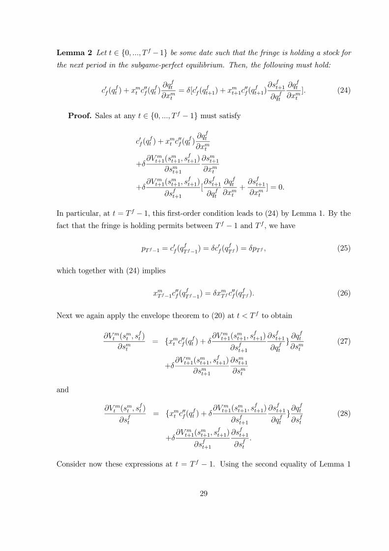
Lemma 2 Let t ∈ {0, ..., T f − 1} be some date such that the fringe is holding a stock forthe next period in the subgame-perfect equilibrium. Then, the following must hold:
c0f(qft ) + xmt c
00f(q
ft )
∂qft∂xmt
= δ[c0f(qft+1) + xmt+1c
00f(q
ft+1)
∂sft+1
∂qft
∂qft∂xmt
]. (24)
Proof. Sales at any t ∈ {0, ..., T f − 1} must satisfy
c0f(qft ) + xmt c
00f(q
ft )
∂qft∂xmt
+δ∂V m
t+1(smt+1, s
ft+1)
∂smt+1
∂smt+1∂xmt
+δ∂V m
t+1(smt+1, s
ft+1)
∂sft+1[∂sft+1
∂qft
∂qft∂xmt
+∂sft+1∂xmt
] = 0.
In particular, at t = T f − 1, this first-order condition leads to (24) by Lemma 1. By thefact that the fringe is holding permits between T f − 1 and T f , we have
pT f−1 = c0f(qfT f−1) = δc0f(q
fT f) = δpT f , (25)
which together with (24) implies
xmT f−1c00f(q
fT f−1) = δxmT f c
00f(q
fT f). (26)
Next we again apply the envelope theorem to (20) at t < T f to obtain
∂V mt (s
mt , s
ft )
∂smt= {xmt c00f(qft ) + δ
∂V mt+1(s
mt+1, s
ft+1)
∂sft+1
∂sft+1
∂qft} ∂q
ft
∂smt(27)
+δ∂V m
t+1(smt+1, s
ft+1)
∂smt+1
∂smt+1∂smt
and
∂V mt (s
mt , s
ft )
∂sft= {xmt c00f(qft ) + δ
∂V mt+1(s
mt+1, s
ft+1)
∂sft+1
∂sft+1
∂qft}∂q
ft
∂sft(28)
+δ∂V m
t+1(smt+1, s
ft+1)
∂sft+1
∂sft+1
∂sft.
Consider now these expressions at t = T f − 1. Using the second equality of Lemma 1
29
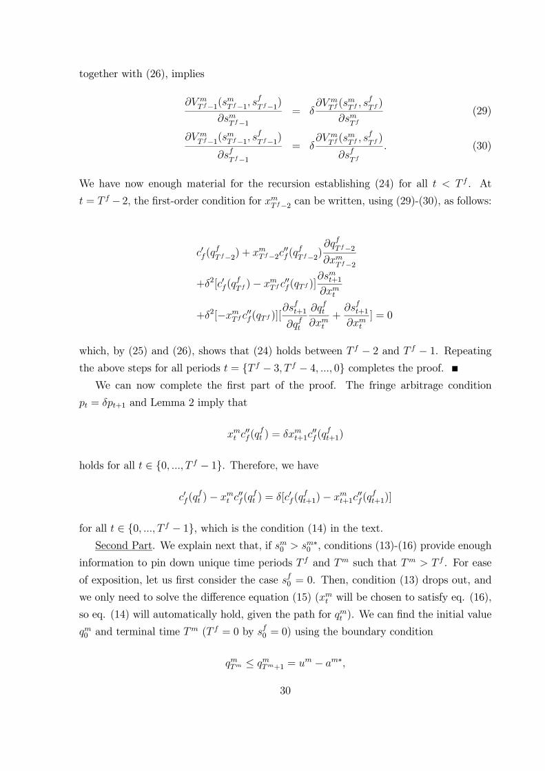
together with (26), implies
∂V mT f−1(s
mT f−1, s
fT f−1)
∂smT f−1
= δ∂V m
T f (smT f , s
fT f)
∂smT f
(29)
∂V mT f−1(s
mT f−1, s
fT f−1)
∂sfT f−1
= δ∂V m
T f (smT f , s
fT f)
∂sfT f
. (30)
We have now enough material for the recursion establishing (24) for all t < T f . At
t = T f − 2, the first-order condition for xmT f−2 can be written, using (29)-(30), as follows:
c0f(qfT f−2) + xmT f−2c
00f(q
fT f−2)
∂qfT f−2
∂xmT f−2
+δ2[c0f(qfT f)− xmT f c
00f(qT f )]
∂smt+1∂xmt
+δ2[−xmT f c00f(qT f )][∂sft+1
∂qft
∂qft∂xmt
+∂sft+1∂xmt
] = 0
which, by (25) and (26), shows that (24) holds between T f − 2 and T f − 1. Repeatingthe above steps for all periods t = {T f − 3, T f − 4, ..., 0} completes the proof.We can now complete the first part of the proof. The fringe arbitrage condition
pt = δpt+1 and Lemma 2 imply that
xmt c00f(q
ft ) = δxmt+1c
00f(q
ft+1)
holds for all t ∈ {0, ..., T f − 1}. Therefore, we have
c0f(qft )− xmt c
00f(q
ft ) = δ[c0f(q
ft+1)− xmt+1c
00f(q
ft+1)]
for all t ∈ {0, ..., T f − 1}, which is the condition (14) in the text.Second Part. We explain next that, if sm0 > sm∗0 , conditions (13)-(16) provide enough
information to pin down unique time periods T f and Tm such that Tm > T f . For ease
of exposition, let us first consider the case sf0 = 0. Then, condition (13) drops out, and
we only need to solve the difference equation (15) (xmt will be chosen to satisfy eq. (16),
so eq. (14) will automatically hold, given the path for qmt ). We can find the initial value
qm0 and terminal time Tm (T f = 0 by sf0 = 0) using the boundary condition
qmTm ≤ qmTm+1 = um − am∗,
30
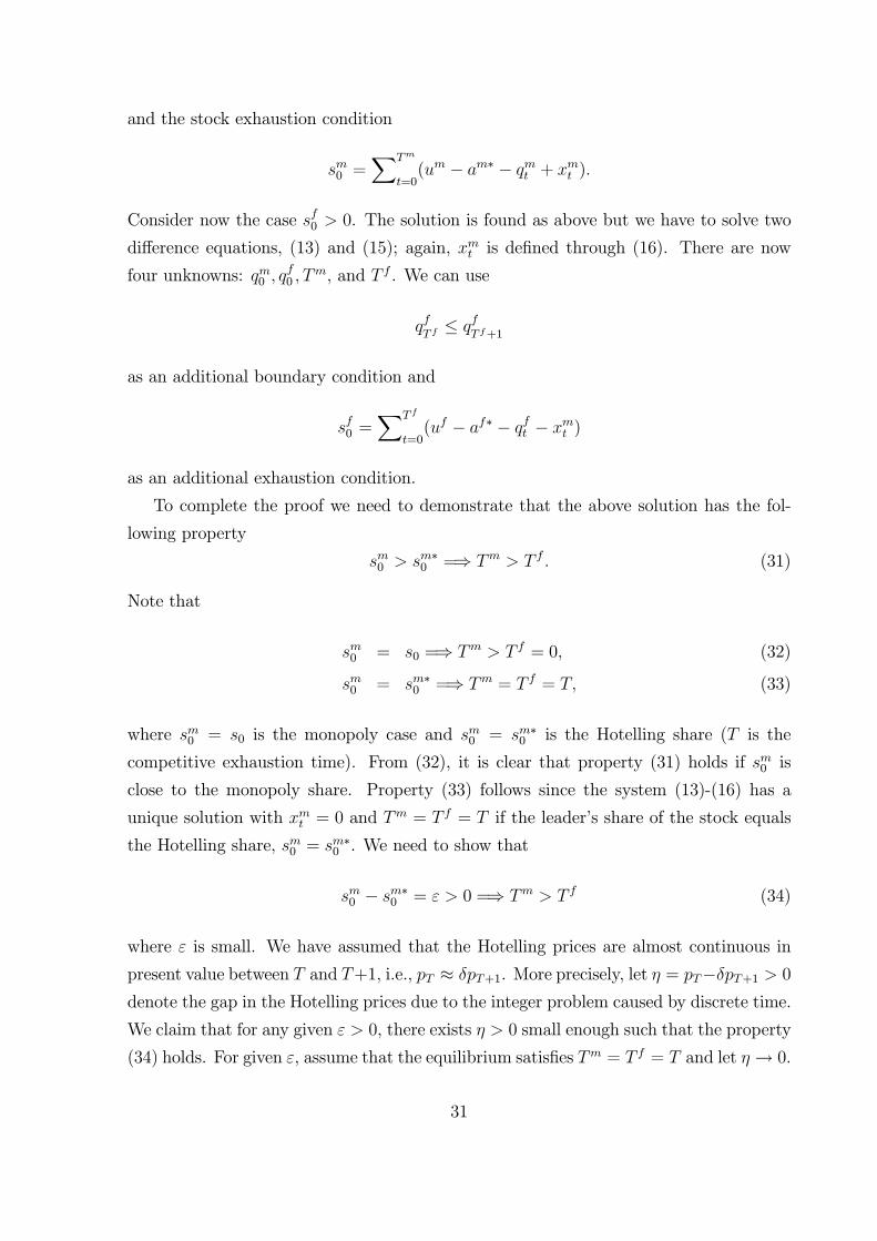
and the stock exhaustion condition
sm0 =XTm
t=0(um − am∗ − qmt + xmt ).
Consider now the case sf0 > 0. The solution is found as above but we have to solve two
difference equations, (13) and (15); again, xmt is defined through (16). There are now
four unknowns: qm0 , qf0 , T
m, and T f . We can use
qfT f≤ qf
T f+1
as an additional boundary condition and
sf0 =XT f
t=0(uf − af∗ − qft − xmt )
as an additional exhaustion condition.
To complete the proof we need to demonstrate that the above solution has the fol-
lowing property
sm0 > sm∗0 =⇒ Tm > T f . (31)
Note that
sm0 = s0 =⇒ Tm > T f = 0, (32)
sm0 = sm∗0 =⇒ Tm = T f = T, (33)
where sm0 = s0 is the monopoly case and sm0 = sm∗0 is the Hotelling share (T is the
competitive exhaustion time). From (32), it is clear that property (31) holds if sm0 is
close to the monopoly share. Property (33) follows since the system (13)-(16) has a
unique solution with xmt = 0 and Tm = T f = T if the leader’s share of the stock equals
the Hotelling share, sm0 = sm∗0 . We need to show that
sm0 − sm∗0 = ε > 0 =⇒ Tm > T f (34)
where ε is small. We have assumed that the Hotelling prices are almost continuous in
present value between T and T+1, i.e., pT ≈ δpT+1. More precisely, let η = pT−δpT+1 > 0denote the gap in the Hotelling prices due to the integer problem caused by discrete time.
We claim that for any given ε > 0, there exists η > 0 small enough such that the property
(34) holds. For given ε, assume that the equilibrium satisfies Tm = T f = T and let η → 0.
31
This leads to a contraction since, by ε > 0, it is an option for the leader to comply without
trading, i.e., equalize marginal costs in present value by using permits from the stock sm0 .
But this implies that the leader has not used ε when period t = T arrives. Selling ε at
t = T leads to pT < δpT+1, which is the contradiction. Reoptimizing at the last period
implies that it becomes optimal to extend the overall depletion period, Tm > T f .
Appendix B: Proof of Proposition 2Proof. The result is proved by backward induction as follows. First, at the exhaustion
period T the equilibrium is shown to be efficient if smT ≤ sm∗T (sm∗t denotes the Hotelling
share at t). Second, at T − 1 the equilibrium is efficient if smT−1 ≤ sm∗T−1. In particular,
the leader’s spot market transaction at T − 1 is such that the exhaustion period stock isalso competitive, smT ≤ sm∗T . Finally, the argument extends to any number of periods to
go, implying that the efficiency follows from sm0 ≤ sm∗0 .
Consider now period T and let smT ≤ sm∗T . Suppose first that the leader is a seller at
the exhaustion period, xmT > 0. Then, the leader’s spot market transaction must be such
that the following hold:
pT = c0f(qfT ) ≥ δc0f(q
fT+1) = δpT+1 (35)
c0f(qfT )− xmT c
00f(q
fT ) = c0m(q
mT ) (36)
≥ δc0m(qmT+1) = δpT+1, (37)
where, by the fact that T is the exhaustion period,
qfT = uf − af∗ − sfT + xmT ,
qmT = um − am∗ − smT − xmT ,
qfT+1 = uf − af∗
qmT+1 = um − am∗.
By the definition of sm∗T , smT = sm∗T implies that condition (36) holds without trading,
i.e., xmT = 0. Therefore, choosing xmT > 0 when smT ≤ sm∗T implies c0m(q
mT ) > pT = c0f(q
fT ),
which contradicts profit maximization.
Thus, the leader must be a buyer, xmT ≤ 0, when the stock is below the Hotelling
share, smT ≤ sm∗T . When there is monopsony power, conditions (35) and (37) must still
32

hold but (36) must be replaced by
max{δpT+1, c0f(qfT )− xmT c00f(q
fT )} = c0m(q
mT )
since the fringe arbitrage implies that their permit values cannot go below δpT+1 =
δc0f(qfT+1) = δc0m(q
mT+1). This in turn implies that the most the leader can do is to depress
the last period price to make the arbitrage condition in the last period, condition (35),
to hold as an equality. We have assumed that the Hotelling prices are almost continuos
in present value between T and T + 1, i.e., pT ≈ δpT+1.41 Since the true price at t = T
is sandwiched between the Hotelling price (achieved exactly when smT = sm∗T ) and δpT+1,
we can ignore the leader’s ability to depress the period T price.
Consider now period T − 1 and let smT−1 ≤ sm∗T−1. Again, selling at T − 1 from a stockbelow the Hotelling share leads to a contradiction with profit maximization because this
would imply
pT−1 < c0m(qmT−1) = δc0m(q
mT ),
where the equality follows from the fact that the leader has an option to store permits.
The leader is thus a buyer at T − 1 and has two options. First, he can buy a quantitythat keeps the stock below the Hotelling share,
0 ≥ xmT−1 ≥ smT−1 − sm∗T−1. (38)
Period T − 1 price cannot be depressed by restricting the purchase, since the fringearbitrage implies
pT−1 = δpT
where the equality follows from the fact that the fringe is storing permits. The equilibrium
is therefore competitive at T − 1 as long as (38) holds. Second, the leader can buy aquantity that raises the holding above the Hotelling share
xmT−1 < smT−1 − sm∗T−1. (39)
Now, the leader is a seller at T and conditions (35)-(37) must hold at T , which is antici-
pated by the market at T − 1. Having observed (39), the fringe arbitrage leads to
pT−1 = δpT > δ2pT+1,
41See footnote 14.
33

where the inequality follows from (35)-(36) together with xmT > 0. However, the leader
is now buying with a price higher than the marginal benefit from buying,
pT−1 = δpT > δ{c0f(qfT )− xmT c00f(q
fT )} = δc0m(q
mT ).
This shows that keeping the stock below the Hotelling share, strategy (38), is optimal at
T − 1. Therefore, the equilibrium is competitive at T − 1, if smT−1 ≤ sm∗T−1.
To complete the proof, we note that the argument for stage T −1 can be repeated forany stage between t = 0 and t = T −1, implying that the subgame-perfect equilibrium iscompetitive if sm0 ≤ s∗m0 . The equilibrium abatement path is unique, although any actual
trading path xmt that is consistent with the per-period compliance requirement and that
keeps the stock below the Hotelling share qualifies as an equilibrium path.
References
[1] Allaz, B., and J.-L. Vila (1993), Cournot competition, forward markets and effi-
ciency, Journal of Economic Theory 59, 1-16.
[2] Babiker, M.H., J.M. Reilly, M. Mayer, R.S. Eckaus, I. Sue Wing and R.C. Hyman
(2001), The MIT Emissions Prediction and Policy Analysis (EPPA) Model: Revi-
sions, Sensitivities, and Comparisons of Results. Report No. 71, Joint Program on
the Science and Policy of Global Change, MIT.
[3] Bernard A., S. Paltsev, J. Reilly, M. Vielle and L. Viguier (2003), Russia’s role in
the Kyoto Protocol, Report No. 98, Joint Program on the Science and Policy of
Global Change, MIT.
[4] Bulow, J. (1982), Durable-good monopolists, Journal of Political Economy 90, 314-
332.
[5] Coase, R. (1972), Durability and monopoly, Journal of Law and Economics 15,
143-149.
[6] Dixit, A. and R. Pindyck (1994). Investment under Uncertainty. Princeton Univer-
sity Press, New Jersey.
34
[7] Ellerman, A.D, P. Joskow, R. Schmalensee, J.-P. Montero, and E.M. Bailey (2000),
Markets for Clean Air: The US Acid Rain Program, Cambridge University Press,
Cambridge, UK.
[8] Ellerman, A.D., and J.-P. Montero (2005), The efficiency and robustness of allowance
banking in the U.S. Acid Rain Program, Working paper, Center for Energy and
Environmental Policy Research, MIT.
[9] Ellerman, A.D. and Decaux, A. (1998), Analysis of post-Kyoto CO2 emissions trad-
ing using marginal abatement cost curves, working paper, Report No. 40, Joint
Program on the Science and Policy of Global Change, MIT.
[10] Ellis, G.M. and R. Halvorsen (2002), Estimation of market power in a nonrenewable
resource industry, Journal of Political Economy 110, 883-899.
[11] Gilbert, R. (1978), Dominant Firm Pricing with Exhaustible Resources, Bell Journal
of Economics 9, 385-395.
[12] Goulder, L., and Mathai, K. (2000), “Optimal CO2 abatement in the presence of in-
duced technological change”, Journal of Environmental Economics and Management
39, 1-38.
[13] Hahn, R. (1984), Market power and transferable property rights, Quarterly Journal
of Economics 99, 753-765.
[14] Hagem, C., and H. Westskog (1998), The design of a dynamic tradable quota system
under market imperfections, Journal of Environmental Economics and Management,
36, 89-107.
[15] Hotelling, H. (1931), The economics of exhaustible resources, Journal of Political
Economy 39, 137-175.
[16] Jacoby, H., R. Schamlensee and I. Sue Wing (1999), Toward a useful architecture
for climate change negotiations, Report No. 49, Joint Program on the Science and
Policy of Global Change, MIT.
[17] Joskow, P., R. Schmalensee and E.M. Bailey (1998), The market for sulfur dioxide
emissions, American Economic Review 88, 669-685.
35
[18] Karp, L. and D. Newbery (1993), Intertemporal Consistency Issues in Depletable
Resources, In Handbook of Natural Resource and Energy Economics vol. 3, A.V.
Kneese and J.L. Sweeney (Eds.), Amsterdam, North Holland.
[19] Lewis, T. and R.Schmalensee (1980), On oligopolistic markets for nonrenewable
resources, Quarterly Journal of Economics 95, 475-491.
[20] Lewis, T. and R.Schmalensee (1982), Cartel deception in nonrenewable resource
markets, Bell Journal of Economics 13, 263-271.
[21] Liski, M. and J.-P. Montero (2005), ”A Note on Market Power in an Emissions Per-
mit Market with Banking,” Special Issue in Environmental and Resource Economics
Vol. 31, No. 2, 159-173.
[22] Liski, M. and J.-P. Montero (2006a), On pollution permit banking and market power,
Journal of Regulatory Economics, forthcoming.
[23] Liski, M. and J.-P. Montero (2006b), Forward trading and collusion in oligopoly,
Journal of Economic Theory, forthcoming.
[24] Manne, A.S.and R.G. Richels (2001), US rejection of the Kyoto Protocol: The
impact on compliance costs and CO2 emissions, mimeo, Stanford University.
[25] Montero, J.-P. (1999), Voluntary compliance with market-based environmental pol-
icy: Evidence from the U.S. Acid Rain Program, Journal of Political Economy 107,
998-1033.
[26] Newbery, D.M. (1981), Oil prices, cartels and the problem of dynamic inconsistency,
Economic Journal 91, 617-646.
[27] Rubin, J.D. (1996), A model of intertemporal emission trading, banking, and bor-
rowing, Journal of Environmental Economics and Management 31, 269-286.
[28] Salant, S.W. (1976), Exhaustible resources and industrial structure: A Nash-
Cournot approach to the world oil market, Journal of Political Economy 84, 1079-
1093.
[29] Schennach, S.M. (2000), The economics of pollution permit banking in the con-
text of Title IV of the 1990 Clean Air Act Amendments, Journal of Environmental
Economics and Management 40, 189-210.
36

[30] Tietenberg, T. (2006), Emissions Trading: Principles and Practice, Resources for
the Future, Washington, DC, forthcoming.
[31] Williams, J. C. and B. D. Wright (1991). Storage and Commodity Markets. Cam-
bridge, UK: Cambridge University Press.
37

cm'(qm)
p
p
Tf Tm t
p*
T
FIGURE 1: Salant's equilibrium path
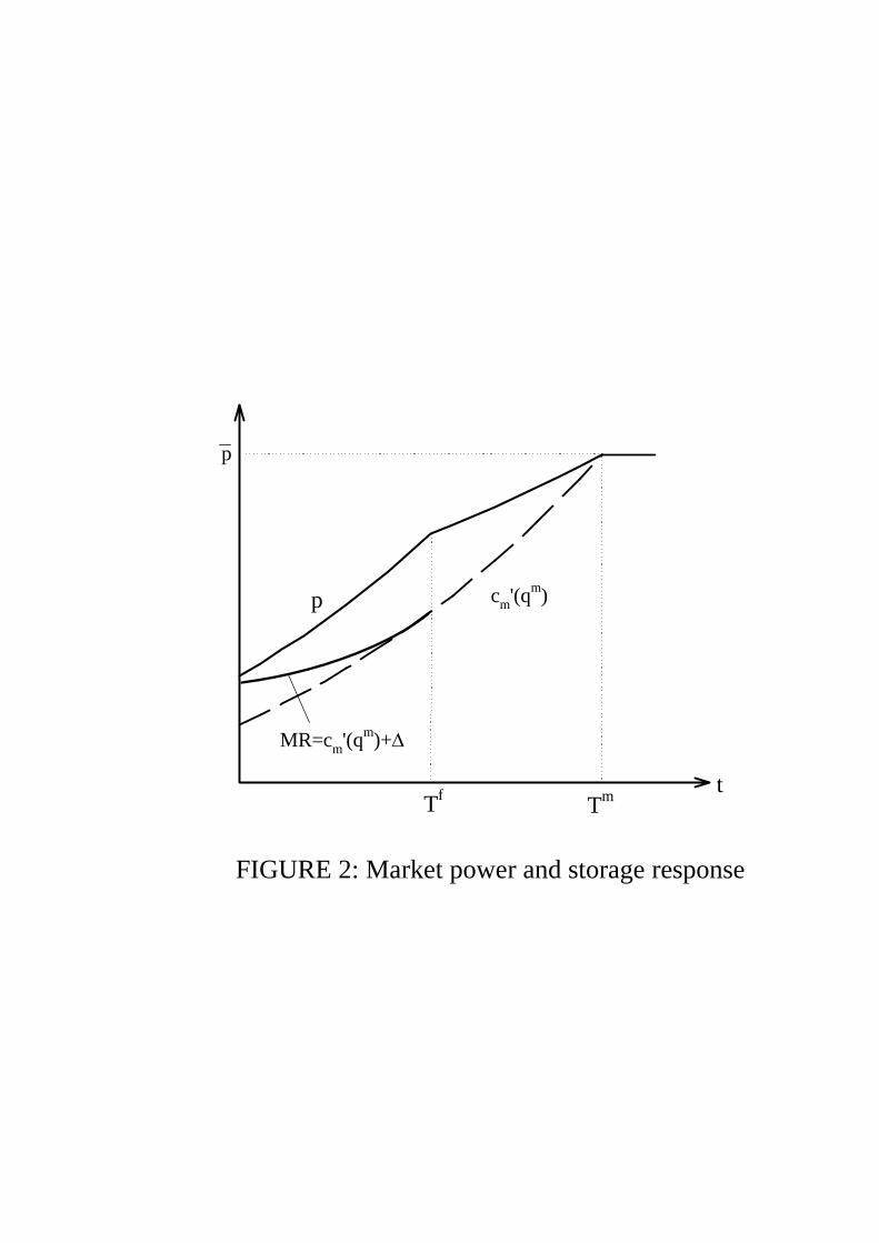
cm'(qm)p
Tf Tm
MR=cm'(qm)+Δ
t
FIGURE 2: Market power and storage response
p
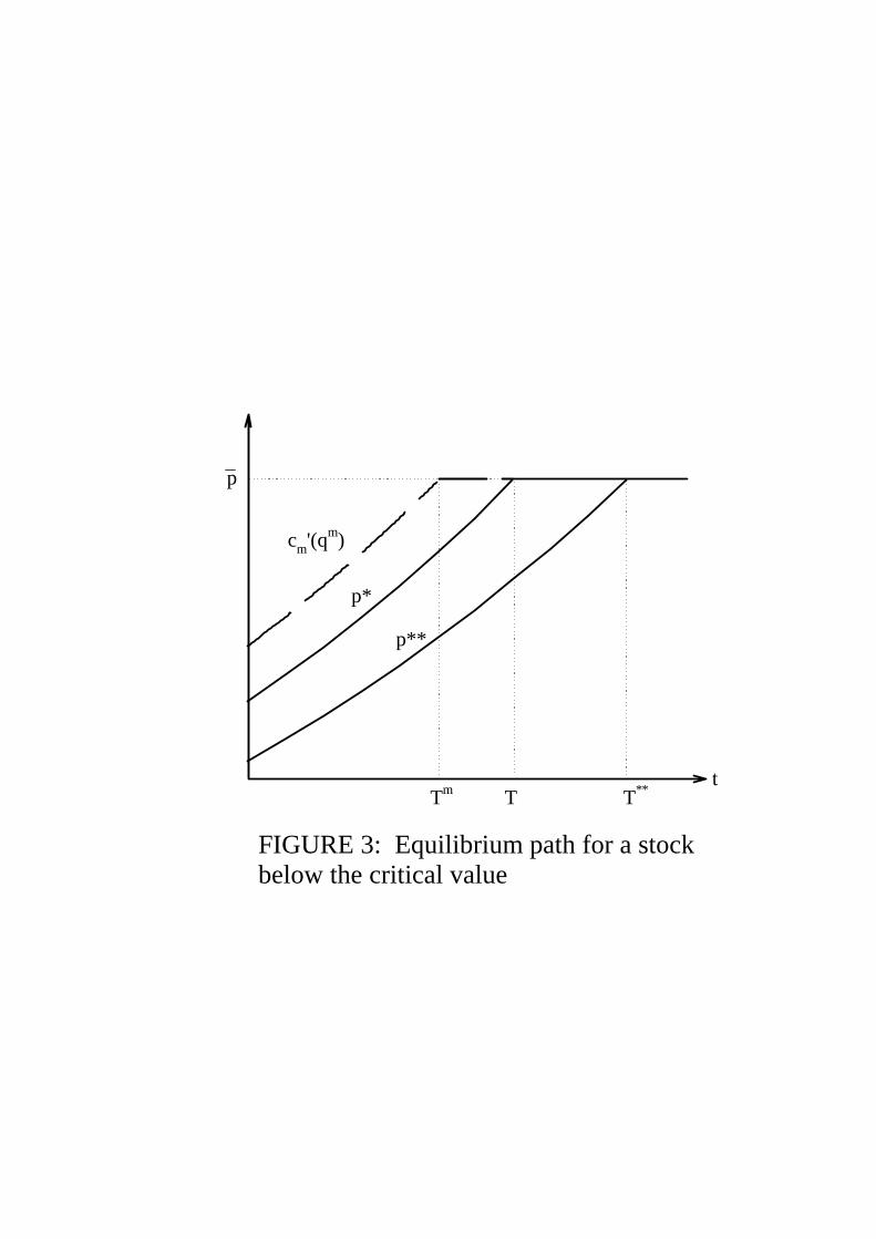
cm'(qm)
p*
p**
t
FIGURE 3: Equilibrium path for a stock below the critical value
T**TTm
p

atm
utm-qt
m*
TT'
C
B
A
FIGURE 4: Allocation path that leads to unwanted market power
tt'

ppm
T0f Tm t
p*
T
p1m
p0m
p*
T1f
FIGURE 5: Long-run monopoly power
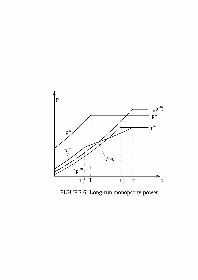
cm'(qm)
p*pm
T0f Tm t
p*
T
p
p1m
p0m
T1f
xm=0
FIGURE 6: Long-run monopsony power

Table 1: Static equilibrium in 2010
___Emissions (mtC)__ ______Permits (mtC)______
Prices ($/tC) OKR FSU Total CDM OKR FSU Total
FSU sales (mtC)
No regulation 2,153 818 2,970 Perfect competition 11.0 2,027 749 2,776 100 1,672 1,004 2,776 255 Maximum market-power 20.1 1,975 818 2,793 135 1,672 1,004 2,811 168
OKR: other Kyoto regions; FSU: Former Soviet Union; CDM: Clean Development Mechanism. Table 2: Perfectly competitive equilibrium path
_Annual Emissions (mtC)_ ____Annual Permits (mtC)____ _Stocks (mtC)_
Year Prices ($/tC) OKR FSU Total CDM OKR FSU Total
FSU (st
m*) Total 2010 62 1816 654 2,470 236 1,672 1,004 2,912 350 442 2015 79 1877 714 2,591 302 1,672 1,004 2,978 639 829 2020 101 1909 754 2,663 386 1,672 1,004 3,062 889 1,228 2025 129 1941 786 2,728 493 1,512 908 2,912 1,010 1,413 2030 164 1970 816 2,785 630 1,366 820 2,817 1,015 1,445 2035 210 2046 856 2,901 806 1,235 742 2,782 901 1,325 2040 268 2112 890 3,002 1,000 1,116 670 2,787 681 1,110 2045 342 2161 912 3,072 1,000 1,009 606 2,615 375 653 2050 436 2191 922 3,113 1,000 912 548 2,460 0 0
TOTALS 18,021 7,304 25,325 5,852 12,168 7,305 25,325 OKR: other Kyoto regions; FSU: Former Soviet Union; CDM: Clean Development Mechanism. Table 3: Perfectly competitive equilibrium path with stock-holding limits
_Annual Emissions (mtC)_ ____Annual Permits (mtC)____ _Stocks (mtC)_
Year Prices ($/tC) OKR FSU Total CDM OKR FSU Total
FSU (st
m*) Total 2010 66 1,805 650 2,455 121 1,672 1,004 2,798 -496 343 2015 84 1,865 709 2,574 155 1,672 1,004 2,831 -201 601 2020 107 1,895 748 2,643 198 1,672 1,004 2,875 54 832 2025 136 1,926 780 2,705 254 1,590 955 2,799 230 926 2030 174 1,952 808 2,760 324 1,512 908 2,744 330 910 2035 222 2,025 847 2,872 414 1,438 863 2,716 346 754 2040 283 2,089 880 2,969 529 1,368 821 2,718 287 503 2045 361 2,135 901 3,035 677 1,301 781 2,758 167 226 2050 461 2,161 910 3,071 865 1,237 743 2,845 0 0
TOTALS 17,851 7,233 25,084 3,538 13,463 8,083 25,084 OKR: other Kyoto regions; FSU: Former Soviet Union; CDM: Clean Development Mechanism.

Table 4: Evolution of largest holding companies’ compliance paths in the sulfur market American Elec. Power Southern Company Group of Four All firms
Year Permits Emissions Permits Emissions Permits Emissions Permits Emissions1995 1,194,410 739,322 1,079,502 534,392 3,607,506 2,049,809 8,694,296 5,298,6171996 1,182,429 926,215 1,079,085 565,097 3,591,282 2,259,687 8,271,366 5,433,3511997 883,634 959,556 991,297 591,411 3,001,934 2,312,083 7,108,052 5,474,4401998 883,634 871,738 991,297 642,093 3,001,728 2,229,636 7,033,671 5,298,4981999 883,634 723,589 991,297 614,790 3,001,809 2,088,510 6,991,170 4,944,6662000 663,514 1,136,095 734,464 1,048,296 2,121,591 3,307,858 9,714,830 11,202,0522001 663,514 998,620 734,464 957,872 2,119,625 3,090,712 9,307,565 10,631,3432002 663,514 979,653 734,464 959,338 2,119,625 3,059,693 9,282,297 10,175,0572003 653,062 1,039,413 728,778 988,245 2,103,487 3,161,696 9,123,376 10,595,9452004 653,062 1,017,878 728,778 969,568 2,103,487 3,096,652 9,123,376 10,432,326
… 2012 653,062 890,164 728,778 847,915 2,103,487 2,708,114 9,123,376 9,123,376
TOTALS Cumulative
by 1999 5,027,741 4,220,420 5,132,478 2,947,783 16,204,259 10,939,725 38,098,555 26,449,572diff. 1999 807,321 2,184,695 5,264,534 11,648,983
Cumulative by 2003 7,671,345 8,374,201 8,064,648 6,901,534 24,668,587 23,559,684 75,526,623 69,053,969
diff. 2003 -702,856 1,163,114 1,108,903 6,472,654Cumulative
by 2012 13,548,903 16,960,388 14,623,650 15,080,208 43,599,970 49,681,131 157,637,007 157,054,629diff. 2012 -3,411,485 -456,558 -6,081,161 582,378


