MARKET INTEGRATION AND PRICING
EFFICIENCY, EMPIRICAL ANALYSES TO THE
AGRIBUSINESS SECTOR
Dissertation
to obtain the Joint Ph. D. degree in Agricultural Economics
at the Faculties of Agricultural Sciences from the
Georg-August-University Göttingen, Germany
and University of Talca, Chile
presented by
Rodrigo Andrés Valdés Salazar
born in Talca, Chile
Göttingen, April 2015
!
!
ii!
D7
1. Name of supervisor in Germany: Stephan Von-Cramon Taubadel, Dr.
2. Name of supervisor in Chile: Alejandra Engler Palma, PhD
3. Name of further members of the examination committee:
3.1 Rodrigo Herrera, Dr.
3.2 Felipe Lillo, PhD
3.3 José Diaz-Osorio, Dr.
Date of dissertation: April 27th 2015
!
!
iii!
For Samanta with Love
!
!
iv!
Acknowledgements
I am most grateful to the Chilean National Commission for Scientific and Technological
Research (CONICYT) and the German Academic Exchange Service (DAAD) for their
financial contribution to the development of my academic career over the past three years.
Though the responsibility of writing this dissertation and the shortcomings therein are
mine, much of the research has essentially been the work of a sustained collaboration and
academic guidance from my supervisors, Prof. Alejandra Engler Palma and Prof. Stephan
von Cramon-Taubadel. I appreciate and gratefully acknowledge the usefulness of their
guidance and collaboration for the development of my thesis. Many thanks again to both
supervisors and through them, to the Departments of Agricultural Sciences from the
University of Talca and Georg-August-University Göttingen.
I appreciate the role of Ms. Antje Wagener and Ms. Ximena Gonzalez, the affables
postgraduate assistants from both universities and all former and present colleagues from
different institutions for their support in which I should like to highlight the role played by
Dr. José Diaz, Dr. Roberto Jara, Dr. Cristian Adasme, Dr. Sebastian Lakner, Dr. Friederike
Greβ, Dr. Linde Götz, Dr. Zoltán Bakucs and Mr. Matthieu Stigler.
I also acknowledge the support during different stages of my thesis to researchers from the
Leibniz Institute of Agricultural Development in Transition Economies (IAMO), the Chair
of Development Economics at the University of Göttingen, the Institute of Economics of
the Hungarian Academy of Sciences (HAS) and to the people at the R lists for answering
my questions regarding programming.
Finally, thanks to all the people that has been involved and helped me to reach this stage, in
special my wife Samanta, my parents, brothers and grandparents, this could not have been
done without their support.
!
!
v!
Contents
List of Figures................................................................................................................vii
List of Tables................................................................................................................. vii
Chapter 1: Introduction ................................................................................................ 1
Chapter 2: Measuring market transaction costs !......................................................... 4
2.1. Transportation, transaction and exchange costs..................................................4 2.2. The cointegration analysis...................................................................................5
Chapter 3: Transaction costs and trade liberalization: An empirical perspective from
the MERCOSUR agreement ........................................................................................10
3.1. Introduction.........................................................................................................12
3.2. Literature review.................................................................................................14
3.3. The relevance of transaction costs in international trade ...................................16
3.4. Estimation strategy..............................................................................................18
3.5. Results and Discussion........................................................................................21
3.6. Concluding remarks............................................................................................29
3.7. Bibliographic References....................................................................................31
Chapter 4: Driving factors of agribusiness stock markets: a panel cointegration
analysis..............................................................................................................................37
4.1. Introduction..........................................................................................................39
4.2. Drivers of regional stock market integration.......................................................41
4.3. Methodology........................................................................................................43
4.4. Data description...................................................................................................45
!
!
vi!
4.5. Empirical results and discussion.........................................................................48
4.6. Conclusion..........................................................................................................56
4.7. References...........................................................................................................57
Chapter 5: Spatial market integration and fuel prices: an empirical analysis of the Chilean horticultural sector.........................................................................................61
3.1. Introduction.......................................................................................................63
3.2. The spatial market integration ..........................................................................64
3.3. Methods ............................................................................................................66
3.4. Data description ................................................................................................68
3.5. Results ..............................................................................................................69
3.6. Discussion.........................................................................................................73
3.7. Conclusions ......................................................................................................75
3.8. Bibliographic References .................................................................................76
!
!
vii!
List of Figures
Figure 1-3. Values of the Gonzalo-Pitarakis sup LMγ Statistics with
respect to the Chilean Fuel Prices ..................................................................................70
List of Tables
Table 1-1. Description of the variables and their MFN tariffs and
market share in the Brazilian market.............................................................................. 21
Table 2-1. Results test on cointegration and lag length for each country pairs according to
the ADF Residual, Johansen-Juselius tests and Akaike Criterion respectively.............. 22
Table 3-1. TVECM Estimation Results for the pre- and post
MERCOSUR periods: Brazil-Argentina........................................................................ 24
Table 4-1. TVECM Estimation Results for the pre- and post
MERCOSUR periods: Brazil-United States................................................................... 25
Table 1-2. List of trade blocs, member countries and their respective
stock markets.................................................................................................................. 46
Table 2-2. Description of the covariates in the stock market integration
model.............................................................................................................................. 47
Table 3-2. Summary statistics and unit root test for the panel variables .......................48
Table 4-2. Correlation matrix for Panel Series of the Model......................................... 49
Table 5-2. Hausman and F tests for model selection of the panel regression.................50
Table 6-2. Estimation results for the models A and B....................................................51
Table 1-3. Description of the variables considered in this study....................................68
Table 2.3. Estimates for the regime dependent VECM..................................................72
!
!
Introduction
!! !
1!
CHAPTER 1.
Introduction
Markets are organizations created to facilitate exchange. This is possible because a market
comprises a set of institutions developed primarily to reduce a particular type of transaction
costs: the market transaction costs. Those costs are important not assess market efficiency,
but also to understand how and in which circumstances two or more markets are
interconnected. They are the key-variable to understand efficiency in economic
organizations.
Transaction costs literature has been widely applied in many different research fields, such
as development, finance, agricultural economics and natural resource economics, among
others. Despite this recognition, measuring transaction costs is still a challenging task. As
Allen (2006) states, if transaction costs could be measured with reasonable accuracy, the
theory would become more valuable. More integrated markets are associated with a higher
degree of relationship-specific assets, prices or more frequent exchange.
Among the empirical methods applied, Richman and Macher (2006) indicate thre main
strategies to analyze transaction cost, namely: (i) the qualitative case studies, (ii)
quantitative single industry studies, and (iii) econometric analyses. In the econometric
analyses, two methods were preferred: (a) time series analysis ; and (b) panel data
estimation. The advantage of the first method is the possibility of correcting the selection
bias associated with estimating the effect of organizational mode on performance (Masten,
1993). The panel data models are useful because they offer many procedures to control
unobservable components.
There is an abounding literature exploring the degree of integration between markets and
trying to measure market transaction costs, among which the cointegration analyses is one
of the most popular. One important shortcoming of this literature is the entanglement of
exchange, transportation and transaction costs, due to the inaccuracy about how these
concepts are defined and quantified. This imprecision has induced the misleading
assumption of transaction costs and, consequently, has yielded an inaccurate measurement
of the latter. Actually, the lack of a standardized transaction costs definition is a
!
!
Introduction
!! !
2!
shortcoming of many attempts in different research fields that have already tried to quantify
them. In order to overcome this issue and by means of cointegration models, this thesis
suggests a different set of procedures to measure market transaction costs in different
agricultural sectors and can be easily replicated to different markets. This procedure also
allows to measuring the exchange and transportation costs associated with a transaction and
the effect transaction cost has on the agricultural sector.
This PhD thesis consists of three papers which explore price transmission and market
efficiency in selected fields of agricultural economics.
The first, investigate whether Brazil became more integrated with reduced transaction costs
after the introduction of MERCOSUR with respect to its main agricultural trade partners,
Argentina (a MERCOSUR member) and the United States (a non-MERCOSUR member).
Using a threshold vector error correction model (TVECM), we estimate the transaction
cost, price transmission elasticity and half-lives adjustments for the most traded agricultural
products between Brazil/Argentina and Brazil/United States from January 1980 to
December 2012.
The second, explores the drivers of regional stock market integration with a focus on the
agribusiness sector across the most important regional trade blocs around the world. Based
on the literature on market integration and stock return pricing, we identify nine possible
determinants of stock market integration, which we separate into three categories:
individual market performance, macroeconomic conditions and agricultural trade. We
implement panel cointegration models to analyze the stock indices of agribusiness firms in
MERCOSUR, EU, APEC and NAFTA. Furthermore, we account for agriculture-specific
factors to control for possible structural shifts in financial markets by including the two
main commodity price bubbles during last 20 years.
Finally, the thid paper propose a procedure to estimate a regime-dependent vector error
correction model with an exogenous threshold variable (Chilean retail fuel prices) were not
only the short and long- run equilibrium relationship itself can display threshold-type non-
linearity. The proposed approach is unique in explicitly testing the threshold cointegration
process based on the Gonzalo and Pitarakis (2006) test. We considered the most relevant
central and regional wholesale markets (Santiago and Talca) the prices of the most planted
Chilean horticultural products, namely: maize, tomato, onion, carrot. In order to account for

!
!
Introduction
!! !
3!
the fuel prices, we consider the Chilean retail prices. The research was conducted using a
price series of weekly frequency for the period January 2009 to December 2013.
!
!
Measuring market transaction cost
!! !
4!
CHAPTER 2.
Measuring market transaction costs !
2.1. Transportation, transaction, and exchange costs
Acoording to Serigati and De Azevedo (2014), exchanging a good is a costly activity. As
well as it is necessary to incur expenses to produce a good, it is also necessary to allocate
resources to market it. According to Coase (1988), market is an institution that exists “to
facilitate exchange”, that is, it exists “in order to reduce the cost of carrying out exchange
transactions”. Thus, we assume for now on that market is an organization created to
facilitate the exchange. It is possible because a market is composed of a set of institutions
that reduce the market transaction costs. Those costs are associated with the necessary
activities to elaborate and to enforce the contract that will intermediate the exchange.
The literature that has tried to measure market transaction costs frequently has considered
those costs synonymous to transportation costs. However, transportation and transaction
costs represent costs of different origins; while transportation costs represent the costs of
transfer physically a good from one market to another, taking into account fuel, freight,
taxes, tariffs, wages, fares, etc., market transaction costs are linked essentially to
information and bargaining costs. Moreover, combined the market transaction costs and the
transportation costs form the exchange costs. This idea is reflected in Benham and Benham
(2001) definition of exchange costs: “the opportunity cost faced by an individual to obtain a
specified good using a given form of exchange within a given institutional setting” .
Higher exchange costs make the trading process more expensive. Actually, they can even
insulate markets. Markets for the same good can be in equilibrium with different prices
because it is costly to ship products from one market to another to take advantage of
arbitrage opportunities triggered by a price difference. It is worth to highlight it is not any
price difference that can consolidate a profitable arbitrage opportunity; this difference must
be higher than (or at least equal to) the exchange costs. Therefore, ceteris paribus, the
higher the exchange costs, the lower is the probability of different markets be integrated.
According to Fackler and Goodwin (2001), “market integration is best thought of as a
!
!
Measuring market transaction cost
!! !
5!
measure of the degree to which demand and supply shocks arising in one region are
transmitted to another region”.
A market reduces exchange costs primarily because it makes the information disclosure
process less costly. As information becomes a cheaper asset, become easier to indentify
possible gains from arbitrage opportunities taking advantage of the price difference in the
two or more markets. Thereby better information flow improves the degree of integration
between different markets. In sum, both transportation and market transaction costs (i.e. the
exchange costs) influence decisively the degree of integration between different markets.
Thus, it is necessary to take them into account to analyze empirically the connection of two
or more markets.
2.2. The cointegration analysis
Many empirical procedures have been applied to study market integration but the
cointegration analysis has been one of the most popular approaches. This literature assumes
the degree of price transmission as a proxy for the level of market integration because it can
‘measure’ the market efficiency in taking advantage of possible arbitrage opportunities.
Interestingly, Marshal’s (1920) market definition gives support to this assumption: similar
goods belong to the same market whenever their prices converge. For the cointegration
literature there is convergence when the prices of those goods share the same long-run
stochastic trend. This convergence means the existence of a long-run equilibrium
influencing the prices behavior in the short run. In this situation, according to Fackler and
Goodwin (2001), market integration is usually a measure of the degree of price
transmission between different markets and market efficiency is used to denote a situation
in which the agents have left no arbitrage opportunities.
There is an important assumption in the linear cointegration models: the prices in the short
run adjust to any deviation in the long-run equilibrium, do not matter how small this change
is. It is a strong assumption because, as we have already discussed previously, the arbitrage
opportunity is profitable only if the price difference is higher than the exchange costs.
Meyer and von Cramon-Taubadel (2004) also criticize the assumption of linear and
symmetric adjustment in cointegration models. According to them, the asymmetric price
!
!
Measuring market transaction cost
!! !
6!
transmissions are more frequently than the symmetric ones due to the presence of: market
power, political intervention, inventory management, adjustment costs (menu costs), and
asymmetric information (different search costs among the agents involved in the
transaction).
Actually, the cointegration literature has already developed non-linear models that
incorporate asymmetric adjustments and exchange costs in its analyses1. Enders and
Granger (1988) is one of the first papers to suggest an approach to evaluate price
transmission equation with asymmetric price adjustments. Balke and Fomby (1997) suggest
a method to incorporate transaction costs in the cointegration models; those models are
known as the threshold cointegration models. Briefly, the threshold cointegration models
incorporate the transaction costs including nuisance parameters linking the equations of the
system. Those nuisance parameters are called thresholds and they allow splitting the system
in different regimes. With different regimes, it is possible to evaluate empirically in which
situations the prices are linked (i.e. in which situations the markets are integrated), how
strong this connection is in each regime, and what the trade flow direction is. Moreover, the
value of each threshold is read as a measure of the transaction costs.
Meyer (2004) proposes a procedure to measure indirectly the transaction costs in currency
values using the threshold influence on the price transmission equation. With the variables
in natural log, the threshold represents how much, in percentage, the deviation has to be
above or below the long-term equilibrium to trigger the regime change. This long-term
equilibrium is calculated substituting the variables in the cointegration vector by their
respective sample mean.
Despite the popularity of the cointegration models, this approach presents several
limitations. In the next paragraphs we focus on the misled concept of transaction costs
applied in this literature. There are also two conceptual inaccuracies in this literature:
• It has employed the concept of transaction costs improperly: what they have
named transaction costs are better expressed by the term exchange costs, the
combination of transportation costs and variable market transaction costs; 1 Asymmetry and exchange costs are not the same thing. The presence of exchange costs can cause asymmetric adjustments, but not all asymmetry is a consequence of exchange costs. However, both can be modeled using the threshold cointegration models. "
!
!
Measuring market transaction cost
!! !
7!
• Besides using the concept of transaction costs far from the Coase’s idea, this
literature use almost only examples of transportation cost to justify the existence of
a persistent price difference. Transportation and transaction costs capture different
aspects of an exchange; they are not synonymous.
It is possible to cite many examples. Bekkerman et al. (2013) employ a definition of
transaction costs close to the idea of exchange costs: “the cost required to transfer a good
from one market to another”. However, when they model those transaction costs, they
select only variables associated with transportation costs like fuel costs and seasonality
components. The same approach is observed in Campenhout (2007) who use transportation
variables (steep passes, road bad conditions, heavy traffic, number of police check posts,
bribes, and costs of living) as proxies for transaction costs. Perhaps ‘bribes’ can be a
reasonable proxy for transaction costs, but his idea about this concept is clearly far from
Coase’s idea: “as expected, the estimated transaction costs are generally proportional to the
distance between two markets”.
Goodwin et al. (2002) and Stephens et al. (2012) justify a threshold effect in the price
transmission because they analyze perishable goods. This is a good proxy for transaction
costs; it can be classified as temporal asset specificity. However, Stephens et al. (2012)
empirically use only transportation costs variables (fuel prices and bus fares) as proxies for
the exchange costs.
There are also papers that justify the existence of transaction costs due to market
characteristics, even when those features are not clearly transaction costs. Rapsomanikis
and Hallam (2006) suggest that adjustment costs in the sugar-ethanol processing industry
and technical factors (the substitution possibilities between ethanol and oil) explain the
existence of transaction costs. Among the market characteristics, Park et al. (2002) cite as
transaction costs variables that are not all really transaction costs (trade restrictions,
infrastructure bottlenecks, managerial incentive reforms, traders skill, market institutions,
the lack of influence of future markets, bribes, and productions specialization policies). But
at least they recognize that markets do not emerge overnight; it can be a long and costly
process.
!
!
Measuring market transaction cost
!! !
8!
Many papers, like Serra et al. (2008) and Serra et al. (2006) model possible transaction
costs without justifying why can be reasonable to consider them. On the other hand,
Balcome et al. (2007) do not present a definition about those costs, but recognize that
transportation and transaction costs are expenses with different origins. Moreover, they also
recognize the existence of fixed and variable exchange costs.
Nowadays, spatial market integration analysis and the role played by transaction costs has a
main role in research and policy making, thus the people conducting such analyses have to
be more aware of the theoretical implications in order to address properly the conclusions
of their empirical work.
2.3. References
Allen, D. 2006. Theoretical Difficulties with Transaction Cost Measurement. Division of
Labor & Transaction Costs (DLTC), Vol. 2, No. 1, pp. 1-14.
Balcombe, K.; Alastair B.; Jonathan B. 2007. Threshold Effects in Price Transmission: The
Case of Brazilian Wheat, Maize, and Soya Prices. American Journal of Agricultural
Economics, Vol. 89, No. 2, pp. 308-23.
Balke, S.; Fomby T. 1997. Threshold Cointegration. International Economic Review, Vol.
38, No. 3, pp. 627–45.
Bekkerman, A.; Goodwin B.; Piggott, N. 2013. Applied Economics, Vol. 45, No. 19, pp.
2705-14.
Benham, A; Benham, L. 2001. The Costs of Exchange. Ronald Coase Institute, Working
Paper Series, No 1, July.
Campenhout, B . 2007. Modelling trends in food market integration - Method and an
application to Tanzanian maize markets. Food Policy, Vol. 32, No. 1, pp. 112–27.
Coase, R. 1988. The Firm the Market and the Law. Pp 1-31 in The Firm, the Market and
the Law, by Ronald H. Coase. Chicago: University of Chicago Press.
Enders, W.; Granger, C. 1998. Unit-Root Tests and Asymmetric Adjustment with an
Example Using the Term Structure of Interest Rates. Journal of Business and Economic
Statistics, Vol. 16, No. 3, pp. 304-311.
Fackler, P.; Goodwin B. 2001. Spatial price analysis. In Gardner, Bruce L., Gordon C.
!
!
Measuring market transaction cost
!! !
9!
Rausser. Handbook of Agricultural Economics, Vol. 1B, ed. B. Amsterdam: Elsevier.
Chapter 17, pp. 971-1024.
Goodwin, B. ;Grennes, T.; Craig, L. 2002. Mechanical Refrigeration and the Integration of
Perishable Commodity Markets. Explorations in Economic History, Vol. 39, No. 2, pp.
154–82.
Marshall, A. 1920. Principles of Economics. Eighth Edition, The Macmillan Company.
London.
Masten, S.; Snyder, E. 1993. United States Versus United Shoe Machinery Corporation: On
the Merits. Journal of Law and Economics, Vol. 36, No. 1, pp. 33-70.
Meyer, J. 2004. Measuring market integration in the presence of transaction costs - a
threshold vector error correction approach. Agricultural Economics, Vol. 31, No. 2-3, pp.
327-34.
Meyer, J.; von Cramon-Taubadel, S. 2004. Asymmetric Price Transmission: A Survey.
Journal of Agricultural Economics, Vol. 55, No. 3, pp. 581-611
Park, A.; Jin, H.; Rozelle, S.; Huang, J. 2002. Market Emergence and Transition -
Arbitrage, Transaction Costs, and Autarky in China’s Grain Markets. American Journal of
Agricultural Economics, Vol. 84, No. 1, pp. 67–82.
Rapsomanikis, G.; Hallam D. 2006. Threshold cointegration in the sugar- ethanol-oil price
system in Brazil: evidence from nonlinear vector error correction models, FAO commodity
and trade policy research working paper No. 22, September.
Richman, B.; Macher, J. 2006. Transaction Cost Economics: An Assessment of Empirical
Research in the Social Sciences. Duke Law School Faculty Scholarship Series. Paper 62.
Serra, T.; Zilberman, D.; Gil, JM. ;Goodwin, B. 2008. Nonlinearities in the US corn-
ethanol-oil price system. Selected Paper prepared for presentation at the American
Agricultural Economics Association Annual Meeting, Orlando, FL, July 27-29.
Serra, T.; Gil, JM.; Goodwin, B. 2006. Local polynomial fitting and spatial price
relationships: price transmission in EU pork markets. European Review of Agricultural
Economics, Vol. 33, No. 3, pp. 415–36.
Stephens, E.; Mabaya, E.; von Cramon-Taubadel, S.; Barrett, C. 2012. Spatial Price
Adjustment with and without Trade. Oxford Bulletin of Economics and Statistics, Vol. 74,
No. 3, pp. 453-69
!
!
Transaction cost and trade liberalization
!! !
10!
CHAPTER 3
Transaction costs and trade liberalization: An empirical perspective from the
MERCOSUR agreement
Rodrigo Valdes a,b,*, Stephan Von Cramon-Taubadel a, Alejandra Engler Palma b
a Georg-August-Universität Göttingen, Department of Agricultural Economics and Rural
Development. Platz der Gottinger Sieben 5, 37073, Göttingen, Germany
b Universidad de Talca. Facultad de Ciencias Agrarias. Departamento de Economia Agraria
y Desarrollo Rural. Casilla 747-721, Talca, Chile.
*Corresponding Author. Universidad de Talca. Facultad de Ciencias Agrarias.
Departamento de Economia Agraria y Desarrollo Rural. Casilla 747-721, Talca, Chile.
Current Address: Tel. +56 71 2200232
Email: [email protected]
Paper submitted to Food Policy
State: received with revisions
!
!
Transaction cost and trade liberalization
!! !
11!
ABSTRACT Studies investigating the effect of trade liberalization policies on transaction costs in
agricultural markets are scarce. The objective of our paper is to determine whether Brazil
became more integrated with reduced transaction costs after the introduction of
MERCOSUR with respect to its main agricultural trade partners, Argentina (a
MERCOSUR member) and the United States (a non-MERCOSUR member).
Using a threshold vector error correction model (TVECM), we estimate the transaction
cost, price transmission elasticity and half-life adjustments for the most traded agricultural
products between Brazil/Argentina and Brazil/United States from January 1980 to
December 2012. Our findings suggest a strong MERCOSUR effect, with lower transaction
costs (TC) and higher price transmission elasticity when compared to a non-agreement
scenario. Moreover, the variations of both parameters are highly heterogeneous across
products, depending mainly on their degree of differentiation. From a policy perspective,
elements such as the sources of comparative and competitive advantages together with
investment policies, specific market regulations and agricultural subsidies, among others,
are mainly what influence the extent of transaction cost and market integration. Our results
show that Brazil has made progress but still has considerable room for improvement in
reducing barriers to agricultural products and, as a consequence, to achieving the full
benefits of the MERCOSUR agreement.
Keywords: Market Integration, Transaction Costs, Threshold Vector Error Correction
Model, Brazil, Argentina, United States.
!
!
Transaction cost and trade liberalization
!! !
12!
1. Introduction Although trade liberalization policies have historically promoted market integration of
regions or countries, recent studies suggest that their effectiveness is negatively affected by
the presence of transaction costs (TCs) (Listorti, 2009, Stephens et al., 2012). In fact, in
order to maximize the benefits from trade liberalization policies, recent studies (Mitra and
Josling, 2009; Martin and Anderson, 2009) argue that countries should take actions to
identify and reduce sources of TCs between markets. A market integration analysis offers a
way to estimate the level of TCs and, consequently, allows for an assessment of whether
regional trade liberalization, under different levels of TCs, affects the price transmission
degree between countries or regions (Balcombe et al. 2007).
While studies of market integration in a spatially separated contexts have received
substantial attention in the literature (e.g. Park et al. [2002] for China; Getnet et al. [2005]
for Ethiopia; Cudjoe et al. [2010] for Ghana and Valdes et al. [2011] for Chile), only a few
studies have explicitly examined the impact of trade agreements on TCs and their
implications for the transmission of price signals between agricultural markets.
The drivers of price transmission include not only the level of trade but also the market
determinants for each country (Koester, 2001). The aim of this study is to explore which
factors affect the degree of market integration, the routes of TC variations derived from the
implementation of regional trade agreements and their effect on the price transmission level
between agricultural markets.
In order to accomplish our objective we used as case study the variation on market
integration parameters of the Brazilian agricultural market with respect to its major trade
partners in both periods: the United States and Argentina, respectively. We used the
implementation of the Common Market of the South (MERCOSUR) as a reference of
structural break in trade. It is expected that after the agreement Brazilian trade will shift
from the United States to Argentina. This study will estimate TCs, price transmission
elasticity (PTE) and their implications for market integration on the top nine agricultural
products traded from 1980 to 2012 between Brazil and the USA (without any trade
agreements) and Argentina and Brazil (existence of a trade agreement).
Previous theoretical studies (see Baulch, 1997 and Blavy and Juvenal, 2009) show that
!
!
Transaction cost and trade liberalization
!! !
13!
transaction costs generate a no-trade threshold band where prices in two locations fail to
equalize. Outside this threshold band, arbitrage is profitable and trade is promoted, a
dynamic that is captured successfully by a threshold vector error correction model
(TVECM) (Balke and Fomby, 1997). This main advantage of this model is its ability to
analyze the impact of TCs on market integration solely on the basis of price information. In
this case the model is capable of identifying a lower bound of the relative TCs associated
with equilibrating price adjustment, e.g., through arbitrage and trade. To the best of our
knowledge, this is the first attempt to relate the impact of regional trade agreements on TCs
and price transmission parameters in agricultural markets.
MERCOSUR is a custom area implemented in 1995 with Brazil, Argentina, Uruguay and
Paraguay as the original partners. Among these countries, Brazil and Argentina generate
more than three-quarters of its agricultural production. Brazil is considered the most
significant agricultural market in Latin America and one of the top 10 players in world
agricultural trade (GVF, 2013). Before the implementation of MERCOSUR, Brazilian
agricultural imports were mainly dominated by the USA, followed by Argentina and the
EU (FAOSTAT, 2013). After the implementation of MERCOSUR, the situation changed
and Argentina became the number one trade partner, followed by the United States,
Venezuela and China (CONAB, 2013). Even though Brazil has fostered trade openness in
order to meet a growing domestic demand for food, there are still signs of high TCs with its
main trade partners (Monteiro et al., 2012). Therefore, there is still no clear evidence about
the effect of trade agreements with respect to the variation of TCs.
Accordingly, this paper attempts to: first, to perform a comparative analysis to determine if
after the implementation of MERCOSUR, TCs between Brazil-Argentina and Brazil-
United States were reduced and if this effect implied a higher PTE; and second, to analyze
whether the formation of TCs and PTE are product-specific and determined by each market
structure.
The article proceeds as follows: Section 2 reviews the Brazilian agricultural market and the
characteristics of MERCOSUR. Section 3 gives a glance at the relevant literature on TCs
and market integration. Section 4 describes the methodology and data sources. Sections 5
and 6 present the results and discussion, respectively. Finally, Section 7 summarizes the
main conclusions.
!
!
Transaction cost and trade liberalization
!! !
14!
2. Literature review
2.1 Brazil in the MERCOSUR context
MERCOSUR is an economic and political treaty, whose members are Brazil, Argentina,
Uruguay, Paraguay and since 2011 Venezuela, while Bolivia and Chile are associate
members2. This custom area consists in a gradual process of tariff harmonization between
these countries with the goal of establishing a common external tariff (CET), which was
finally achieved in early 1995 (Bas, 2012). Today, duty-free access is provided to all goods
produced within the zone with the exception of automobiles and sugar. Along with the
establishment of a CET, the agreement allowed for the free movement of goods, services
and production factors, the abolition of restrictions over reciprocal trade, adoption of
common trade policies towards countries that do not belong to MERCOSUR and the
coordination of macroeconomic and sectorial policies. In 2012, agriculture accounted for 32% of total member exports, 9% of which
corresponding to intra-trade among MERCOSUR countries (FAOSTAT, 2013). According
to Korinek and Melatos (2009), this situation could be due to MERCOSUR’s limited effect
on developing comparative advantages among its members and the fact that when the CET
was established its member economies were engaging trade liberalizations agreements with
other markets simultaneously. As a result, trade with non-member countries was not
affected and in some cases it even grew. At a regional level, MERCOSUR’s agricultural market size is largely determined by Brazil
(Protil et al., 2010). Regarding Brazilian imports, before the implementation of
MERCOSUR the principal provider was the United States (18%), followed by Argentina
(17%), the EU (14%), Uruguay (8%) and Paraguay (6%). At the time, the main Brazilian
imports were wheat (17%), malt (8%), cotton (6%), potatoes (6%) and agro-industry inputs
(4%) (FAOSTAT, 2013). In contrast, after the implementation of MERCOSUR’s,
Argentina has become the biggest exporter of agricultural products to Brazil (24%),
followed by the United States (18%), Venezuela (14%) and China (17%) (CONAB, 2013).
Currently, Brazil’s imports have continued to be dominated by wheat and its derivatives 2 On June 28, 2012, Paraguay was barred from participating in MERCOSUR decisions until it held democratic elections. On July 30, 2012 in Brasilia, the other countries and full members of MERCOSUR approved the final incorporation of Venezuela as a full member, which became effective on August 12, 2012.
!
!
Transaction cost and trade liberalization
!! !
15!
(19%), but barley (11%), fresh fish (6%), beans (7%) and fresh pears (7%) have joined the
list (FAOSTAT, 2013).
2.2 Main agricultural trade policies of the United States and Argentina
Since the United States is one of the biggest players in the global agricultural market, its
main trade policies (namely, market development, export subsidies and market access
programs) may have an important effect on price behavior and arbitrage activities in major
agricultural markets around the world (Mitra and Josling, 2009). This situation is reinforced
by the country’s ample internal logistic network, which allows it to transport agricultural
products to international markets cheaply and efficiently (Korinek and Melatos, 2009),
allowing the United Sates to have competitive advantages in access and product shipping,
that in turn should result in lower TCs.
Brazil and the United States have a long history in terms of agricultural trade. Before the
implementation of MERCOSUR, the United States was the main exporter of agricultural
products to Brazil, as mentioned above. In 2010, both countries signed an agreement for
trade and economic cooperation, a joint effort to promote mutual trade and investment
(Coelho, 2009). As a result, in 2012, Brazil became the seventh largest goods export market
for the United States, totaling $1.9 billion (Sumner, 2013). Current leading categories
include: wheat (US$1.2 billion), dairy products (US$83 million), prepared food (US$67
million), and feeds and fodders (US$51 million) (CONAB, 2013).
On the other hand, Argentina is the eighth largest producer and the twelfth exporter of
agricultural commodities in the world. In 2012 it produced 8.4% of global agricultural
output and its products represent, on average, 2.9% of world agricultural trade during the
last decade (FAOSTAT, 2013). Nevertheless, when compared to the United States, its
transportation and marketing costs for bulk agricultural product exports have historically
been much higher (Brum and Kettenhuber, 2008). This is largely due to an inefficient or
underdeveloped barge and railroad transportation system and a heavy reliance on more
expensive truck hauling that reduces the country’s competitive advantage.
Argentina’s trade policy has historically been one of protectionism, emphasizing import
substitution (Bas, 2012). Due to the hyperinflations of 1989 and 1990, the Argentinean
!
!
Transaction cost and trade liberalization
!! !
16!
government was forced to shift towards market-oriented policies and launched an ample
unilateral trade-liberalization process to promote exports. These policy changes included
trade liberalization, deregulation, privatization of many state enterprises, the MERCOSUR
implementation and a currency convertibility program3 which allowed a significant
expansion of exports (Sturzenegger and Salazni, 2007). As a result, during 2012, Argentina
exported 47% of the world’s soybean oil, 11% of soybeans, 7% percent of wheat and 5%
percent of fresh beef (GVF, 2013).
Policies engaged by both Brazilian partners have had a history of considerable differences
that target TCs in opposite directions. While the United States encourages trade by
reinforcing logistics networks and generates incentive to open markets, Argentina has
crated barriers along the years that translate into a less favorable trade capacity (Nogues
and Porto, 2007). In the case of Argentina, these actions include an export tax, initially at
15%, to restrict exports of meat and dairy products and a complex compensation scheme
for wheat and corn to allow domestic users buy these grains at a more favorable price than
that available to exporters. These situations clearly affect the level of efficiency in which
the tariff and non-tariff advantages of MERCOSUR are implemented between member
countries.
3. The relevance of transaction costs in international trade
Price theory literature has provided wide theoretical evidence about the lack of convergence
of international prices due to the presence of transaction costs (TCs) (Gonzalez-Rivera and
Helfand, 2001; Juvenal and Taylor, 2008). Therefore, not incorporating TCs in the analysis
could distort estimations of degree of integration and convergence among markets or
regions (Meyer and Von Cramon-Taubadel, 2004). Following the definition given by
Barrett (2001), TCs between a market “i” and “j” are composed of transportation costs (fij),
where distance is one of the most important factors; variable costs (vij) associated with
3 The currency convertibility program was designed to eliminate the main source of inflationary pressures, that is, the creation of money to finance the public sector deficit. The convertibility program consisted of a currency board that fixed a nominal relation of one Argentine peso to one U.S. dollar. The currency board was required to provide full backing in U.S. dollars for any issue of Argentine pesos. Moreover, the U.S. dollar was established as legal tender within Argentina. !
!
!
Transaction cost and trade liberalization
!! !
17!
rates, cargo insurance, contracts, financial expenses, hedging, sanitary and phytosanitary
barriers; customs duties (dij); and unmeasurable costs (wij), such as opportunity cost, the
cost of searching for information and risk premiums. Lence and Falk (2005) show that the implementation of trade agreements reduces TCs,
generating higher price transmission and therefore a higher integration of the markets.
According to these authors, this situation increases the levels of market efficiency and
welfare gains mainly due to a closer alignment with the equilibrium condition expressed in
the Enke-Samuelson-Takayama-Judge Model (ESTJ).4 Along the same lines, Barrett (2005)
highlights that welfare gains are directly related to the minimization of TCs, because when
these are expressive and/or trade barriers are effective, the economy is deprived of the
benefits of specialization in trade. His conclusion is supported by Alam et al. (2012), who
analyzed market integration between five major rice markets in Bangladesh. Their results
highlight the importance of shaping policies to reduce TCs, in order to create greater
market efficiency among regional markets.
From an empirical point of view, different components of TCs have been tested for their
impact on market integration. For instance, Aker (2008) found that in Niger, where road
density5 and the quality of products are low, the TCs associated with accessing markets
tend to be higher for grain than for other markets. Moreover, Pingali (2005) suggests that
perishable crops, like vegetables, are usually associated with high TCs when compared to
non-perishable products.
The studies that most resemble our work are those of Meyer and Von Cramon-Taubadel
(2004) and Amikuzuno (2009). The first studied the effects of TCs on the spatial
integration of the pork market between Germany and Holland, concluding that higher TCs
results in a lower arbitrage and therefore lower market integration. According to the
authors, ignoring TCs in the econometric analysis can lead to erroneous conclusions in
terms of the degree of price transmission between countries. The second study analyzed the
implications of trade liberalization on market integration between tomato producers and
consumer markets during periods of high and low agricultural import tariffs in Ghana. This 4 The equilibrium concept at the heart of most trade theory is that of Enke-Samuelson-Takayama-Judge (ESTJ): spatial equilibrium, in which the dispersion of prices in two locations for an otherwise identical good is bounded from the top via the cost of arbitrage between the two markets. Trade volumes are unfettered and bounded from below when trade volumes reach a certain ceiling value. 5 Aker (2008) defines road density as the ratio of the length of the country's total road network to the country's land area.!
!
!
Transaction cost and trade liberalization
!! !
18!
author found that the speeds of price adjustment were higher after import tariffs were
lowered. Looking at a specific trade agreement, Blavy and Juvenal (2009) investigated the
market integration level in sectorial real exchange rate dynamics between Mexico, Canada
and the United States for the periods before and after NAFTA. Their results show that
prices adjusted much faster in the post- NAFTA period mainly because of lower TCs
between each country pair.
In Brazil, studies have mainly focused on the analysis of market integration parameters for
individual sectors or products. For example, González-Rivera and Helfand (2001) analyzed
the integration of Brazilian rice markets. The authors demonstrated that distance and
quality contribute to the formation of TCs between major Brazilian domestic markets.
Coelho (2009) studied the integration of internal and external cotton markets in order to
estimate the influence of trade liberalization on price transmission. His results show that the
Brazilian and U.S. markets are perfectly integrated. Similar to González-Rivera and
Helfand (2001), this author concluded that transport logistics and infrastructure availability
directly contribute to increasing market integration through higher levels of price
transmission.
Our work fills a gap in the current literature by comparing the effect on TCs and PTE using
two country pairs: Brazil-Argentina, with a long history of trade agreements; and Brazil-
United States that, on the contrary, although they a have long term trade relationship do not
possess any long-term agreements. The chosen countries make for a valid comparison case
study because they rank among the top players in the global agricultural market.
4. Estimation strategy 4.1 Model description
In order to estimate TCs and PTE in this paper we applied a regime-dependent model called
Threshold Vector Error Correction Model (TVECM) (Balke and Fomby, 1997). More
precisely, we estimated TVECM models for each price pairs between Brazil-Argentina and
Brazil-United States during the pre- and post- MERCOSUR periods.
The main advantages of TVECM are that: a) prior identification of causality between
analyzed price series is not necessary; b) the timeline of the price transmission process, and
!
!
Transaction cost and trade liberalization
!! !
19!
therefore, of market integration, can be identified; and c) it includes elements that
positively influence the price transmission analysis, for example, deterministic trends,
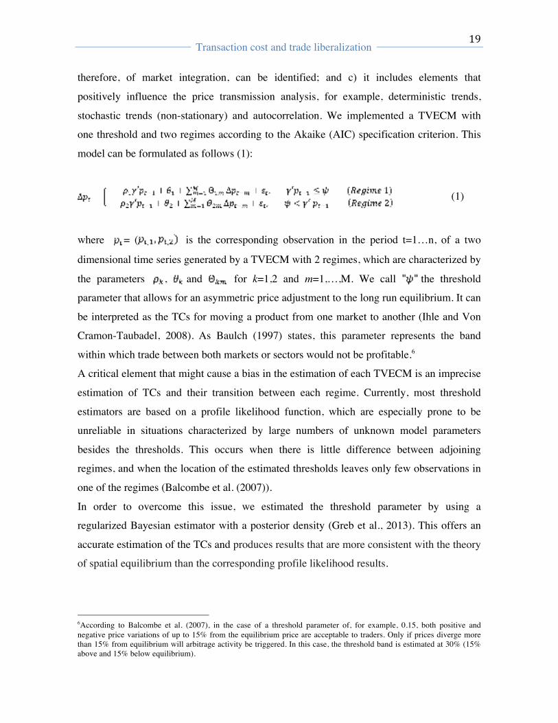
stochastic trends (non-stationary) and autocorrelation. We implemented a TVECM with
one threshold and two regimes according to the Akaike (AIC) specification criterion. This
model can be formulated as follows (1):
(1)
where = ( is the corresponding observation in the period t=1…n, of a two
dimensional time series generated by a TVECM with 2 regimes, which are characterized by
the parameters , and for k=1,2 and m=1,…,M. We call the threshold
parameter that allows for an asymmetric price adjustment to the long run equilibrium. It can
be interpreted as the TCs for moving a product from one market to another (Ihle and Von
Cramon-Taubadel, 2008). As Baulch (1997) states, this parameter represents the band
within which trade between both markets or sectors would not be profitable.6
A critical element that might cause a bias in the estimation of each TVECM is an imprecise
estimation of TCs and their transition between each regime. Currently, most threshold
estimators are based on a profile likelihood function, which are especially prone to be
unreliable in situations characterized by large numbers of unknown model parameters
besides the thresholds. This occurs when there is little difference between adjoining
regimes, and when the location of the estimated thresholds leaves only few observations in
one of the regimes (Balcombe et al. (2007)).
In order to overcome this issue, we estimated the threshold parameter by using a
regularized Bayesian estimator with a posterior density (Greb et al., 2013). This offers an
accurate estimation of the TCs and produces results that are more consistent with the theory
of spatial equilibrium than the corresponding profile likelihood results.
6According to Balcombe et al. (2007), in the case of a threshold parameter of, for example, 0.15, both positive and negative price variations of up to 15% from the equilibrium price are acceptable to traders. Only if prices diverge more than 15% from equilibrium will arbitrage activity be triggered. In this case, the threshold band is estimated at 30% (15% above and 15% below equilibrium).
!
!
Transaction cost and trade liberalization
!! !
20!
Market integration was analyzed by the traditional price transmission elasticity (PTE) and
its corresponding half-life coefficient. While the first is the long run equilibrium parameter
( , the second depends on the adjustment speed of the model’s outer regime ( ) and is
defined as the time required for the effect of 50% of a price shock to phase out. It is
calculated by the equation: ln (0.5)/ln( ).
Prior to the TVECM estimation, we conducted the Elliot-Rothemberg-Stock (ERS) and
Kwiatkowski–Phillips–Schmidt–Shin (KPSS) tests for non-stationarity. In addition, we
tested for the presence of cointegrating vector(s) for all price series by using the Johansen-
Juselius and ADF Residual test procedures simultaneously. We also conducted the Hansen
and Seo test (2002) of linear vs. threshold cointegration. We tested heterogeneity,
autocorrelation and non-normality with the Alexandersson SNHT, Breusch-Godfrey LM
and Lomnicki-Jarque-Bera tests, respectively.
4.2. Data
We used the monthly domestic Brazilian and international FOB prices (in U.S. dollars/ton)
for the top nine agricultural products traded between Brazil-Argentina and Brazil-United
States from January 1980 to December 2012, resulting in 6244 observations.
Domestic Brazilian prices were converted from Brazilian Reals to U.S. Dollars using free
exchange rates (GVF, 2013). All prices series were converted to natural logarithm prior to
estimation and testing. Additionally, previous authors suggest that wheat quality, expressed
by the protein content, plays an important role in the arbitrage mechanism between milling
industries (Brum and Kettenhuber, 2008). We therefore separated wheat price series
according to the protein content of the varieties from Argentina and the United States, that
is, 11% and 12% for PAN (in the case of Argentina) and 11% and 15% for Hard Red
Winter and Soft Red Winter (in the case of the United States).
The data was obtained from the Brazilian National Supply Company (CONAB), the
Economic Institute of the State of Sao Paulo (IESP-Brazil), the United States Department
of Agriculture (USDA), the U.S. Wheat Associates (USW) and the Argentine Association
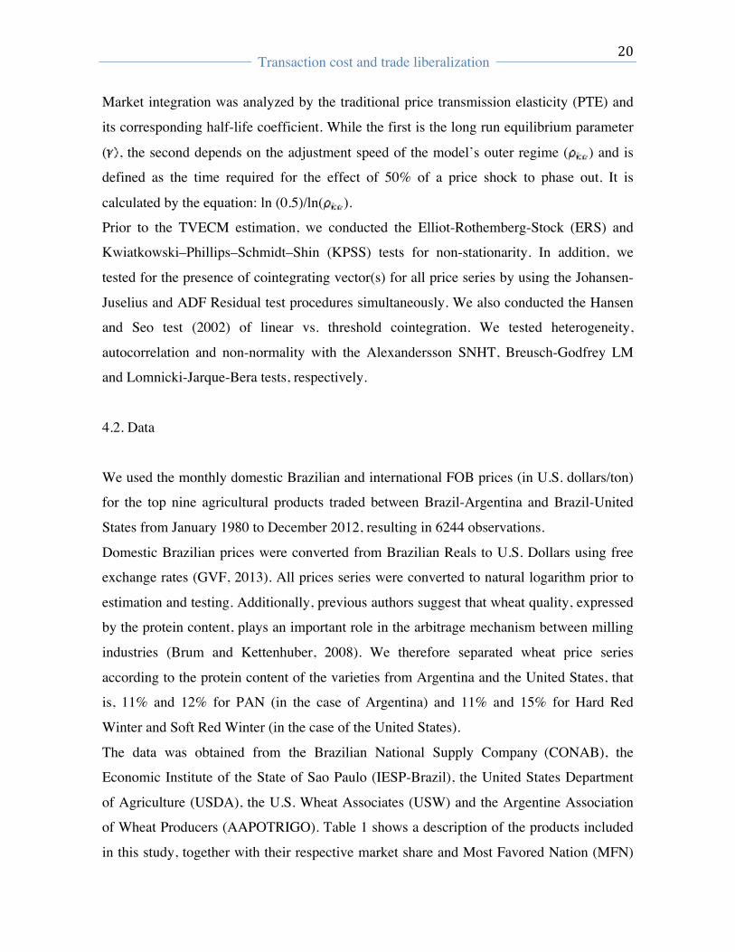
of Wheat Producers (AAPOTRIGO). Table 1 shows a description of the products included
in this study, together with their respective market share and Most Favored Nation (MFN)
!
!
Transaction cost and trade liberalization
!! !
21!
tariffs in the Brazilian market.
Table 1. Description of the variables and their MFN tariffs and market share in the
Brazilian market
Trade Partner HS Code Description Variable
1980-2012 Average % Share Total Agricultural
Imports
2012 MFN tariff (%)
2012 Country Share on this HS Code
(%)
ARGENTINA 100190 PAN 10% protein Pan10 41.5 0 58
ARGENTINA 100190 PAN 12 % protein Pan12 ARGENTINA 110100 Wheat Flour Whf 8.5 12 87 ARGENTINA 110710 Malt Mlt 6.1 14 35
ARGENTINA 7133 Beans (Kidney and White) Kwb 3.1 10 39
ARGENTINA 80820 Pears Fresh Pef 2.9 10 72 ARGENTINA 200570 Olives Oli 2.5 14 65 ARGENTINA 100300 Barley Bar 2.2 7 85 ARGENTINA 40221 Milk Powders Mlp 1.9 14 74
USA 100190 HRW 11% protein Hrw11 41.5 10 21
USA 100190 SRW 15% protein Srw15 USA 210690 Food Preparations Fop 6.2 13 36 USA 520100 Cotton Cot 4.9 8 66 USA 230990 Animal Feed Anf 3.3 8 16 USA 200990 Vegetable Juices Vgj 2.0 14 94 USA 382370 Industrial Alcohols Ina 1.7 2 13 USA 200520 Potatoes Pot 1.5 10 44 USA 100300 Barleys Bar 2.2 12 3
Source: Prepared by the authors with information from Brazilian Customs Service (2012) and FAOSTAT (2013) Note: All price series were converted to natural logs prior to estimation and testing.
5. Results and Discussion
5.1 Preliminary tests
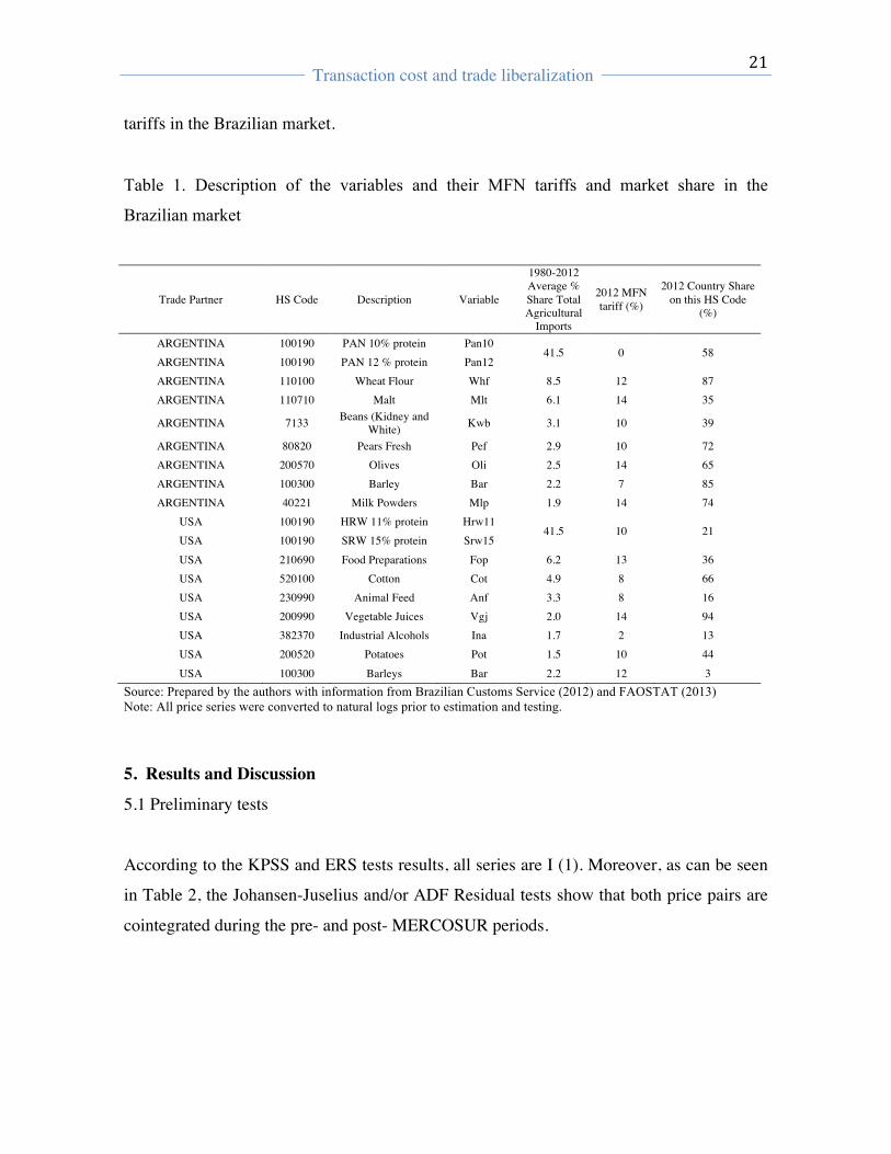
According to the KPSS and ERS tests results, all series are I (1). Moreover, as can be seen
in Table 2, the Johansen-Juselius and/or ADF Residual tests show that both price pairs are
cointegrated during the pre- and post- MERCOSUR periods.
!
!
Transaction cost and trade liberalization
!! !
22!
Table 2. Results test on cointegration and lag length for each country pairs according to the
ADF Residual, Johansen-Juselius tests and Akaike Criterion respectively.
Pre-MERCOSUR Post-MERCOSUR
Variables ADF Residual Based Test
Johansen-Juselius Trace Test, r=0
Lag length
ADF Residual Based Test
Johansen-Juselius Trace Test, r=0
Lag length
Brazil-Argentina Pan10 (-) 4.012*** 19,50 ** 4 (-) 2,001* 20,46 *** 5
Pan12 (-) 2.165* 18,90 * 4 (-) 2.221* 21.65 ** 3 Whf (-) 2.356* 31.44*** 2 (-) 3.331** 42.55*** 2 Mlt (-) 5.115** 21.44** 2 (-) 7.556** 31.55*** 2 Kwb (-) 6.511*** 22.35** 2 (-) 4.331** 16.53* 3 Pef (-) 2.569* 17.33* 3 (-) 3.761*** 18.31* 2 Oli (-) 7.541*** 22.55** 1 (-) 5.233*** 31.23*** 2 Bar (-) 3.892** 15.55* 1 (-) 4.213** 21.34** 1 Mlp (-) 3.949** 16.01* 2 (-) 2.188* 12.01* 2
Brazil-United States Hrw11 (-) 3.790*** 15,20 * 2 (-) 2,256* 24,08** 4 Srw13 (-) 6.015*** 31.08 *** 4 (-) 3.087** 45.77 *** 3 Fop (-) 1,077 13.22 * 4 (-) 2,141* 22.18 ** 2 Cot (-) 3,790*** 18.55 ** 4 (-) 5,610*** 44.71 *** 4 Anf (-) 2.998* 36.99 *** 4 (-) 3.755** 39.01 *** 5 Vgj (-) 3,265** 21.45 ** 2 (-) 4,647*** 18.54 * 4 Ina (-) 4,767*** 27.86 *** 3 (-) 2,183* 29.37 *** 2 Pot (-) 3,681** 16.03 ** 3 (-) 4,771*** 15.13 * 4 Bar (-) 4,888*** 37.66 *** 2 (-) 5,782*** 41.71 *** 2 *, ** and *** indicate statistical significance at the 10%, 5% and 1% levels, respectively
In order to test whether the non-linear specification is superior, we used the Hansen and
Seo test. This test shows statistical significance favoring a non-linear specification.
Ultimately, the residuals did not present heterogeneity and autocorrelation. All test results
are available upon request.
5.2. Model results and discussion
5.2.1 Transaction Costs
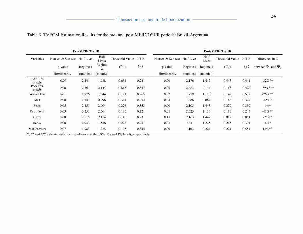
Table 3 and 4 shows evidence of a strong MERCOSUR effect for the Brazil-Argentina and
Brazil-United States pairs. It is worth noting that the reduction in TCs occurs both in
Argentina, a member of MERCOSUR, and in the United States, which is not a member of
this treaty. Moreover, it is important to notice that TCs formation appears to be product-
!
!
Transaction cost and trade liberalization
!! !
23!
specific and highly heterogeneous. Our findings also suggest that the heterogeneity in TCs
among products also translate into a heterogeneous change in TCs by each product in the
list, a finding previously reported in the work of Blavy and Juvenal (2009).
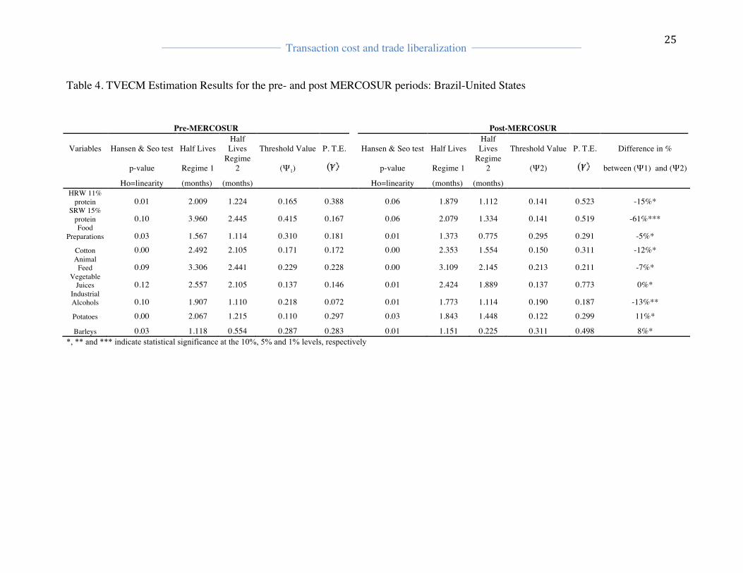
When comparing absolute values during both periods, the Brazil-United States pair
presented lower threshold values than Brazil–Argentina. One explanation is derived from
the policy strategies implemented in both countries, as described in section 2.2. In
particular, the effect of a more open trade policy from the United States during the last 30
years specially facilitates the logistic infrastructure for agricultural imports and exports,
which resulted in lower absolute TCs compared to Argentina.
!
!
Transaction cost and trade liberalization
!! !
24!
Table 3. TVECM Estimation Results for the pre- and post MERCOSUR periods: Brazil-Argentina
*, ** and *** indicate statistical significance at the 10%, 5% and 1% levels, respectively
Pre-MERCOSUR Post-MERCOSUR
Variables Hansen & Seo test Half Lives Half Lives Threshold Value P.T.E. Hansen & Seo test Half Lives Half
Lives Threshold Value P. T.E. Difference in %
p-value Regime 1 Regime 2 (Ψ1) ( p-value Regime 1 Regime 2 (Ψ2) ( between Ψ1 and Ψ2
Ho=linearity (months) (months) Ho=linearity (months) (months) PAN 10%
protein 0.00 2.441 1.988 0.654 0.221 0.00 2.176 1.447 0.445 0.441 -32%** PAN 12%
protein 0.00 2.761 2.144 0.813 0.337 0.09 2.683 2.114 0.168 0.422 -79%***
Wheat Flour 0.01 1.976 1.344 0.191 0.265 0.02 1.779 1.113 0.142 0.572 -26%** Malt 0.00 1.541 0.998 0.341 0.252 0.04 1.286 0.889 0.188 0.327 -45%*
Beans 0.05 2.451 2.004 0.276 0.353 0.00 2.105 1.445 0.279 0.339 1%* Pears Fresh 0.03 3.251 2.664 0.186 0.221 0.01 2.625 2.114 0.110 0.243 -41%**
Olives 0.08 2.515 2.114 0.110 0.231 0.11 2.163 1.447 0.082 0.854 -25%* Barley 0.00 2.033 1.558 0.223 0.251 0.01 1.831 1.225 0.215 0.331 -4%*
Milk Powders 0.07 1.987 1.225 0.196 0.344 0.00 1.103 0.224 0.221 0.551 13%**
!
!
Transaction cost and trade liberalization
!! !
25!
Table 4. TVECM Estimation Results for the pre- and post MERCOSUR periods: Brazil-United States
Pre-MERCOSUR Post-MERCOSUR
Variables Hansen & Seo test Half Lives Half Lives Threshold Value P. T.E. Hansen & Seo test Half Lives
Half Lives Threshold Value P. T.E. Difference in %
p-value Regime 1 Regime
2 (Ψ1) ( p-value Regime 1 Regime
2 (Ψ2) ( between (Ψ1) and (Ψ2)
Ho=linearity (months) (months) Ho=linearity (months) (months) HRW 11%
protein 0.01 2.009 1.224 0.165 0.388 0.06 1.879 1.112 0.141 0.523 -15%* SRW 15%
protein 0.10 3.960 2.445 0.415 0.167 0.06 2.079 1.334 0.141 0.519 -61%*** Food
Preparations 0.03 1.567 1.114 0.310 0.181 0.01 1.373 0.775 0.295 0.291 -5%*
Cotton 0.00 2.492 2.105 0.171 0.172 0.00 2.353 1.554 0.150 0.311 -12%* Animal
Feed 0.09 3.306 2.441 0.229 0.228 0.00 3.109 2.145 0.213 0.211 -7%* Vegetable
Juices 0.12 2.557 2.105 0.137 0.146 0.01 2.424 1.889 0.137 0.773 0%* Industrial Alcohols 0.10 1.907 1.110 0.218 0.072 0.01 1.773 1.114 0.190 0.187 -13%**
Potatoes 0.00 2.067 1.215 0.110 0.297 0.03 1.843 1.448 0.122 0.299 11%*
Barleys 0.03 1.118 0.554 0.287 0.283 0.01 1.151 0.225 0.311 0.498 8%* *, ** and *** indicate statistical significance at the 10%, 5% and 1% levels, respectively
!
!
Transaction cost and trade liberalization
!! !
26!
Taking Barrett’s definition (2001) as a reference, the decrease on threshold values could be a
consequence of a reduction in the formative components of TCs after MERCOSUR. These
components, namely non-tariff barriers, customs procedures, certain phytosanitary measures,
transport and storage times may have all been reduced or relaxed, thus promoting greater or
faster access to the Brazilian market.
Taking a further look at sectorial characteristics, however, it is difficult to establish that the
implementation of MERCOSUR resulted in a constant development of competitive advantages
between Argentina and Brazil. Relative inefficiencies in logistic aspects, due to the lack of
permanent investment policies in infrastructure, have affected the level of efficiency in the
supply chain for most of the agricultural products traded between both countries7. This
situation clearly affects the extent to which those countries take advantage of the tariff and
non-tariff benefits of MERCOSUR.
It is worth noticing that after the treaty the range between the highest and lowest TCs
decreased. For the Brazil-Argentina pair during the pre-MERCOSUR period, threshold values
ranged from 11% (olives) to 81% (PAN wheat 11% protein), while after the agreement came
into force, TCs were reduced to a range from 8.1% (olives) to 44.5% (PAN wheat 10%
protein), 5.5 times the value.
On the other hand, for the Brazil-United States pair, after the MERCOSUR, the biggest
reductions were for high protein HRW and SRW wheat, industrial alcohol (a product traded in
a sector subject to high levels of taxation) and cotton (a highly subsidized producer sector)
(Ben-kaabia et al. 2005; Kupfer, 2011).
During this period, the average reduction in TCs in the case of Brazil-United States was 10 %
when compared to Brazil-Argentina, with a 26% reduction. These results could be used as
evidence to conclude that the agreement did have a real impact on TCs, and could explain the
shift in Brazilian imports from United States to Argentina after the MERCOSUR came into
force.
Now, if we examine the pathways of TCs reduction between a member (Brazil) and a non-
member (USA) of MERCOSUR after 1995. One approach is to analyze the terms of trade
between Brazil and the United States during post- MERCOSUR period. Previous authors
(Maggian and Felipe, 2009; Donoso et al. 2011) confirmed that MERCOSUR created 7 For a detailed discussion of this issue, see Maggian and Felipe (2009), Kupfer (2011) and reference therein.
!
!
Transaction cost and trade liberalization
!! !
27!
increased investment and trade opportunities in Latin America. In particular, Coelho (2009)
reported that exports of differentiated agricultural products from non-members to Brazil
increased significantly from 1995. Since Brazil and Argentina share similar comparative
advantages in a wide group of agricultural products and the structure of comparative and
competitive advantages among Brazil, Argentina and United States are highly asymmetric,
thus it is not surprising a reduction pattern of TCs between Brazil and the United States after
1995. This situation happens mainly because Argentina and Brazil could avoid trading with
each other in agricultural products in which their comparative advantage structure is similar,
allowing to open or maintain the market share of US agricultural products in Brazilian market.
Within this context, since the TCs formation is product specific, the arbitrage between Brazil
and the United States could be promoted by the competitive position of the United States on
products subject to price differentiation or product specificity. For example, considering the
importance of wheat quality on its price formation and according our model's results, we infer
that Brazilian importers chose the US varieties over Argentinean products independently of
the existence of MERCOSUR, because of the higher protein content of HRW and SRW
compared to PAN varieties (Brum and Kettenhuber, 2008), thus driving more intense exports
to important flour producer, such as Brazil.
5.2.2. Price transmission elasticity and half-life coefficients
As described in the methodology section, the TVECM captures the market integration pattern
through a joint estimation of TCs and PTE coefficients. Additionally, from the price
adjustment parameters, we estimates the half-life adjustments to shocks, which represents the
speed at which shocks the variables respond to return the long run equilibrium.
Comparing both country pairs before the implementation of MERCOSUR (Tables 3 and 4), it
can be seen that the average PTE for Brazil-Argentina is lower than for the Brazil-United
States pair. This result suggests that, even though Argentina is closer geographically, the
United States leads the international prices for a diverse group of agricultural products and
thus generates a higher integration among countries.
As in the case of TC, PTE and half-life are product-specific, with higher PTEs for more
differentiated products such as milk powder, industrial alcohol and/or vegetables juices. Half-
!
!
Transaction cost and trade liberalization
!! !
28!
life estimates suggest faster adjustments among these types of products. This is a standard
result in the literature, reported in studies for other country pairs (see Juvenal and Taylor,
2008).
Similarly to TCs dynamics, PTE and half-life coefficients suggest a major market integration
effect after MERCOSUR, with a higher magnitude for Brazil-Argentina than Brazil-USA. In
both cases, while PTE was greater after MERCOSUR, half-life coefficients were lower during
this period. This implies that reduced arbitrage costs were accompanied by faster adjustments
in price differential. It also confirms previous evidence (Barrett (2005) and Ghoshray (2010))
that a common border condition promotes faster price signals among markets. Furthermore,
although PTE presented variability across products, as in the case of TCs, after the agreement
this variability was reduced, suggesting that the price pairs adjust faster, regardless of the size
of the shock. Overall, we managed to identify a pattern of greater price convergence for
Brazil-Argentina than for Brazil-USA, confirming that there is greater market integration
when trade agreements exist
As highlighted in Liefert et al. (2010), there is an inverse relation between the domestic
production and the elasticity of price signals from exporter to importer countries. This
evidence is particularly representative in the case of Brazil-Argentina, in which a higher price
transmission in olives (+73%) and wheat flour (+54%) was found after 1995. For the first one,
since Brazil has a low domestic production, this situation could trigger a more elastic reaction
of Brazilian importers during high demand periods. Similarly, for the case of wheat flour, high
internal demand from the Brazilian milling industry could drive higher levels of PTE after
MERCOSUR.
The highest half-life reductions after MERCOSUR on both country pairs were found on
powdered milk (1.103 months) and fresh pears (2.625 months). In both cases, the domestic
production of Argentina is higher than Brazil and the United States. In fact, during 2012
Argentina occupied the 4th and 6th position among the global exporters of these products
respectively (FAOSTAT, 2013). It is clear that Argentina can offer these products at lower
relative prices than Brazilian producers, generating and asymmetric supply behavior between
both countries. These findings confirm the role played by the domestic production of the
importer countries on the transmission of price signals between countries (Gilhoto and Sesso,
2010).
!
!
Transaction cost and trade liberalization
!! !
29!
For the Brazil-United States pair, higher PTE changes occur for more differentiated products,
such as industrial alcohol (+61%) and vegetable juices (+81%). Interestingly, in the case of
wheat the PTE was higher for the United States varieties, that is, HRW11 (0.523) and SRW 15
(0.519) than for the Argentinean PAN 10 (0.441) and PAN 11 (0.422). Following Maggian
and Felipe (2009), the explanations for these results could be twofold. First, the United States
is a price leader for global wheat prices while Argentina is only a price follower; and second,
infrastructural problems in Argentina and its lack of storage capacity, which probably limits
the arbitrage activities from Argentina to Brazil.
Overall, our study highlights the importance of TCs in international trade and how it can be
affected by trade agreements. The model estimates confirm that when TCs are reduced
integration between markets increases, reinforcing the impact on trade. What is more, the
results for the Brazil-United States pair also suggest that as long as TCs decrease, integration
among markets will increase.
One explanation could be that the asymmetries among the structure of comparative and
competitive advantages between both country pairs and the tariff reduction generated by
MERCOSUR allows a decrease in the TCs level. Nevertheless, MERCOSUR also possesses
an area related to sanitary and phytosanitary issues, that could also be relevant in the formation
of total TCs. This analysis could translate into further research to determine which results
could be of high relevance for policy makers.
In spite of the most relevant sources of TCs, the aforementioned results suggest that policies
oriented to reducing internal trade barriers, such as having an efficient logistic infrastructure or
expedite sanitary and phytosanitary inspections and procedures, could provide efficient
measures to reduce TCs and impact trade in a positive manner. On the contrary, it is highly
probable that having internal barriers that increase TCs will prevent full exploitation of the
trade agreement, reducing its impact on member countries.
6. Concluding remarks
We used a TVECM in order analyze the effect of MERCOSUR on TCs and market integration
between the Brazil/Argentina and Brazil/USA country pairs. Our findings confirmed a
!
!
Transaction cost and trade liberalization
!! !
30!
significant MERCOSUR effect with lower TCs and higher PTE after the implementation of
this customs area for most of the products considered in the study.
Our results suggest a positive effect on trade flows and arbitrage activities in the agri-food
sectors for both country pairs, with highly heterogeneous TC and PTE variations across
products. For both cases the TC reduction pattern was product-specific. It was higher for
differentiated products, such as high protein wheat, powdered milk, industrial alcohol and
vegetables juices, among others. With respect to PTE, the highest increases for most of the
products occurred during the post-MERCOSUR period in the Brazil/Argentina pair,
confirming the positive role played by distance in the transmission of price signals.
In the case of Brazil/Argentina, the lower expression of TCs could occur because of two
formative components of these costs, such as variable costs and possible reductions in custom
duties that effectively promoted greater efficiency in the process of Brazilian imports from
Argentina. In the case of Brazil/USA, our results suggest that TC reductions occur in two
forms: first, MERCOSUR could create increased investment and trade opportunities through
access to a larger market, such as Brazil; and second, because MERCOSUR countries could
trade products in which they do not have strong comparative advantages among themselves,
and reserve trade in products in which the United States has a comparative advantage.
From our results, it was possible to conclude that MERCOSUR, despite its duty-free access,
has produced fewer trade opportunities for member countries compared to non-members for
some specific products. This situation is mainly because a lack of transport and
communications infrastructure dampens trade opportunities and competitiveness arising from
the MERCOSUR agreement. Therefore, it appears that Argentina’s membership in
MERCOSUR alone is unlikely to be sufficient in overcoming its physical or economic trade
barriers compared to the United States.
In conclusion, Brazil and Argentina have considerable room to maximize the benefits of
MERCOSUR through the implementation of policies to develop logistics, transportation and
internal distribution mechanisms. There is an opportunity to enhance competition and
productivity between domestic producers and reduce the remaining barriers to external trade.
Some of the more sensitive issues, such as subsidy policies, have not been addressed at a
regional level, which has also affected the efficiency of the implementation of MERCOSUR.
For example, the export tax in Argentina on some agricultural products has created some
!
!
Transaction cost and trade liberalization
!! !
31!
distortions in trade flows with Brazil despite the existence of a duty-free area. Clearly, this
diminishes the competitiveness of Argentine exports and makes room for highly competitive
countries who are price makers in the global market, such as the United States.
Finally, future research could focus on analyzing whether the level of subsidies affects TCs
between agricultural markets, mainly focusing on the role of market structure and regulations
on the integration pattern.
Acknowledgements
We are grateful for the helpful comments of two anonymous referees and the constructive
encouragement of the editor during the preparation of this article.
We also acknowledge the useful suggestions in earlier drafts from Jorge Retamales Aranda
and Guillermo Schmeda-Hirschmann. Funding for this research comes from the Chilean
Commission for Scientific and Technological Research (CONICYT)-Folio No. 21120286.
7. Bibliographic References
Aker J., 2008. Droughts, Grain Markets and Food Crisis in Niger. Available at SSRN:
http://ssrn.com/abstract=1004426 or http://dx.doi.org/10.2139/ssrn.1004426. Accessed
20.03.2012.
Alam M., McKenzie A., Buysse J., Begum I., Wailes E., Van Huylenbroeck G., 2012.
Measuring Market Integration in the Presence of Threshold Effect: The Case of Bangladesh
Rice Markets. Selected Paper prepared for presentation at the Agricultural & Applied
Economics Association 2012 AAEA Conference, Seattle, Washington.
Amikuzuno J., 2009. Spatial Price Transmission and Market Integration in Agricultural
Markets after Liberalization in Ghana: Evidence from Fresh Tomato Markets. Ph.D. Thesis,
Faculty of Agricultural Sciences, Georg-August University Goettingen, Germany, 160 P.
Balcombe, K., A. Bailey, and J. Brooks. 2007. Threshold effects in price transmission: the
case of Brazilian wheat, maize, and soya prices. American Journal of Agricultural Economics
89(2): 308–323.!
!
!
Transaction cost and trade liberalization
!! !
32!
Balcombe, K., & Rapsomanikis, G., 2008. Bayesian estimation and selection of nonlinear
vector error correction models: the case of the sugar-ethanol-oil nexus in Brazil. American
Journal of Agricultural Economics, 90(3), 658-668.
Balke N., Fomby, T., 1997. Threshold cointegration. International Economic Review 38, 627–
645.
Barrett C., 2001. Measuring integration and efficiency in international agricultural markets.
Review of Agricultural Economics 23 (1), 19-32.
Barrett C., Li J., 2002. Distinguishing Between Equilibrium and Integration in Spatial Price
Analysis. American Journal of Agricultural Economics 84 (2), 292-307.
Barrett C., 2005. Spatial market integration. Cornell University. Available
on:<http://aem.cornell.edu/faculty_sites/cbb2/Papers/PalgraveSpatialMarketIntegration.pdf>.
Accessed 14.01.2013.
Bas, M. 2012. Input-trade liberalization and firm export decisions: Evidence from Argentina.
Journal of Development Economics, 97(2), 481-493.
Baulch, B., 1997. Transfer Costs, Spatial Arbitrage, and Testing for Food Market Integration.
American Journal of Agricultural Economics 79, 477-487.
Blavy R., Juvenal L., 2009. Mexico’s Integration into NAFTA Markets: A View from Sectoral
Real Exchange Rates. Federal Reserve Bank of St. Louis Review 91(5), 441-64.
Brum A., Kettenhuber P., 2008. A realidade da cadeia do trigo no Brasil: o elo
produtores/cooperativas. Revista de Economia e Sociologia Rural 46 (1), 145-169.
Ben-kaabia M, Gil J.M., Ameur M., 2005. Vertical integration and non-linear price
adjustments: the Spanish poultry sector. Agribusiness 21 (2), 253- 271.
Brazilian Customs Service, 2012. Sistema de Informações Jurídico-Tributárias – SIJUT.
Available on http://www.receita.fazenda.gov.br/Aplicacoes/Atbsa/sijut/default.htm. Accessed
16.10.2012.
Coelho A., 2009. A cultura do algodão e a questão da integração entre preços internos e
externos. Universidade de São Paulo, São Paulo, SP. Working Paper 34 (3), 33-45.
Companhia Nacional de Abastecimento do Brasil (CONAB). 2013. Exportações brasileiras.
Principais produtos de origem agropecuária. Available at www. conab.gov.br.
Cudjoe G., Breisinger C., Diao X., 2010. Local impacts of a global crisis: food price
transmission, consumer welfare and poverty in Ghana. Food Policy 35, 294–302.
!
!
Transaction cost and trade liberalization
!! !
33!
Donoso C., Larson D., Thompson S., 2011. Regional Market Integration and MERCOSUR:
Implications for Wheat Trade. Contributed Paper at the International Food and Agribusiness
Management Association Meeting, Sydney, Australia.
Fackler P., Goodwin B., 2001. Spatial Price Analysis. Handbook of Agricultural Economics 1
(7), 973-1021.
FAOSTAT, 2013. Statistics, Agricultural Trade, Internet Database. http://www.fao.org/faostat
. Accessed 22.04.2013.
Franceschi L., Benin G., Guarienti E., Marchioro V., Martin T., 2009. Pre-harvest factors that
affect wheat technological quality. Ciência Rural 39 (5), 1624-1631.
Getulio Vargas Foundation (GVF). 2013. Brazilian Agricultural Statistics Database. Available
on www.fgv.br.
Getnet K., Verbeke W., Viaene, J., 2005. Modeling spatial price transmission in the grain
markets of Ethiopia with an application of ARDL approach to white teff. Agricultural
Economics 33, 491–502.
González-Rivera G. Helfand S., 2001. The Extent, Pattern, and Degree of Market Integration:
A Multivariate Approach for the Brazilian Rice Market, Amer. J. Agr. Econ. 83 (3), 576-592.
Götz L., Glauben T., Brümmer B., 2013. Wheat export restrictions and domestic market
effects in Russia and Ukraine during the food crisis. Food Policy 38, 214–226
Greb F., von Cramon-Taubadel S., Krivobokova T., Munk A., 2013. The Estimation of
Threshold Models in Price Transmission Analysis. Am. J. Agr. Econ. 95 (4), 900-916.
Ghoshray A., 2010, Smooth transition effects in price transmission: The case of international
wheat export prices. Economic Letters 106 (3), 169–171.
Guilhoto J., Sesso U., 2010. Estimação da Matriz Insumo-Produto Utilizando Dados
Preliminares das Contas Nacionais: Aplicação e Análise de Indicadores Econômicos para o
Brasil em 2005. Economia & Tecnologia 6 UFPR/TECPAR.
Hummels, D. , Lugovskyy, V. and Skiba, A. 2009. The trade reducing effects of market power
in international shipping. Journal of Development Economics 89 (1), 84-97.
Ihle, R., and S. v. Cramon-Taubadel. 2008. A Comparison of Threshold Cointegration and
Markov-Switching Vector Error Correction Models in Price Transmission Analysis.
Proceedings of the NCCC-134 Conference on Applied Commodity Price Analysis,
!
!
Transaction cost and trade liberalization
!! !
34!
Forecasting, and Market Risk Management. St. Louis, MO.
[http://www.farmdoc.uiuc.edu/nccc134]. 22 P.
Inter-American Development Bank (IDB)., 2003. The Impacts of US Agricultural and Trade
Policy on Trade Liberalization and Integration via a US-Central American Free Trade
Agreement. Working Paper -SITI- 04, 52 pp.
Juvenal L., Taylor M., 2008. Threshold Adjustment of Deviations from the Law of One Price.
Studies in Nonlinear Dynamics and Econometrics 12(3), 34-66
Koestler U., 2001. Market Integration: How it Works. Research Report. International Food
Policy Research Institute. Washington, D. C. 15 P.
Korinek, J., Melatos M. 2009. Trade Impacts of Selected Regional Trade Agreements in
Agriculture. OECD Trade Policy Working Papers, No. 87, OECD publishing
Kupfer, D., 2011. Competitividade da indústria brasileira: visão de conjunto e tendências de
alguns setores. Revista Paranaense de Desenvolvimento-RPD 82, 45-78.
Lence S., Falk B., 2005. Cointegration, Market Integration and Market Efficiency. Journal of
International Money and Finance 24, 873-890.
Liefert W., Liefert O., Vocke G., Allen E., 2010. Former Soviet Union Region to play
larger role in meeting world wheat needs. Amber Waves 8 (2), 12–19.
Listorti G., 2009. Testing International Price Transmission under Policy Intervention. An
Application to the Soft Wheat Market. Associazione Alessandro Bartola. PhD Studies Series
6, Ancona.
Maggian R., Felipe I., 2009. Aspects of competitiveness of wheat chain in Brazil and in
Argentina. Sociedade Brasileira de Economia, Administração e Sociologia Rural, 47th Sober
Congress.
Martin W., Anderson K., 2011. Export Restrictions and Price Insulation during Commodity
Price Booms. Policy Research Working Paper No. 5645, World Bank, Washington, DC.
Meyer J., Von Cramon-Taubadel S., 2004. Asymmetric Price Transmission: A Survey. Journal
of Agricultural Economics 55, 581-611.
Mitra S., Josling T., 2009. Agricultural Export Restrictions: Welfare Implications and Trade
Disciplines. IPC Position Paper Agricultural and Rural Development Policy Series.
International Food & Agricultural Trade Policy Council.
!
!
Transaction cost and trade liberalization
!! !
35!
Monteiro, G., Farina, E., Nunes, R. 2012. Food‐Retail Development and the Myth of
Everyday Low Prices: The Case of Brazil. Development Policy Review, 30(1), 49-66.
Nogues, J., Porto, A., 2007. Duties and restrictions on agro-industrial exports. Working Paper
No. 25. Forum of the Argentine Agro-industrial Chain. Faculty of Economics and Agro-
industrial Forum Convention, UNLP.
Park A., Jin H., Rozelle S., Huang J., 2002. Market emergence and transition: Arbitrage,
transaction costs, and autarky in China’s grain markets. American Journal of Agricultural
Economics 84 (1), 67–82.
Pingali, P., Khwaja, Y., Meijer, M., 2005. Commercializing small farms: reducing transaction
costs. ESA Working Paper No. 05-08. Agricultural and Development Economics Division,
Food and Agriculture Organization, Rome.
Protil R., Pedro J., Calsavara S., 2010. Government Policies and the Wheat Chain
Coordination in Brazil. 48th Congresso da Sociedade Brasileira de Economia, Administração
e Sociologia Rural, Curitiba.
Rapsomanikis G., Hallam D., 2006. Threshold cointegration in the sugar- ethanol-oil price
system in Brazil: evidence from nonlinear vector error correction models. FAO Commodity
and Trade Policy Research Working Paper No. 22, Rome, Italy.
Stephens E., von Mayaba E., Cramon-Taubadel S., Barrett, C., 2012. Spatial price adjustment
with and without trade. Oxford Bull. Econ. Stat. 74 (3), 453–469.
Sturzenegger, A., Salazni, M. 2007. Distortions to Agricultural Incentives in Argentina.
Agricultural Distorsions Research Project, Working Paper 10, World Bank Publishing.
Sumner, D. 2003. Implications of the US Farm Bill of 2002 for agricultural trade and trade
negotiations. Australian Journal of Agricultural and Resource Economics 47 (1), 99-122.
Tang, D. 2005. Effect of Regional Trading Arrangements on Trade: Evidence from NAFTA,
ANZCER and ASEAN Countries, 1989-2000. Journal of International Trade and Economic
Development, 14 (2), 241-265.
Valdes R., Cramon-Taubadel S., Diaz-Osorio J., Engler A., 2011. Market integration for
Chilean wheat prices using Vector Error Correction Models (VECM), a cointegration analysis.
Ciencia e Investigación Agraria, 38(1), 5-30.
!
!
Transaction cost and trade liberalization
!! !
36!
Vasconcelos S., 2012. Os efeitos da carga tributária indireta e das políticas públicas agrícolas
sobre os preços dos alimentos em Porto Alegre (RS), Brasil. Revista de Economia e
Sociologia Rural, 50 (4), 34-4.
!
!
Driving factors of agribusiness stock markets
!! !
37!
CHAPTER 4
Driving factors of agribusiness stock markets: a panel cointegration analysis
Rodrigo Valdes a,b,*, Stephan Von Cramon-Taubadel a , Alejandra Engler b
a Georg-August-Universitat Gottingen, Department of Agricultural Economics and Rural
Development. Platz der Gottinger Sieben 5, 37073, Gottingen, Germany
b Universidad de Talca. Facultad de Ciencias Agrarias. Departamento de Economia Agraria.
Casilla 747-721, Talca, Chile.
*Corresponding Author. Universidad de Talca. Facultad de Ciencias Agrarias. Departamento
de Economia Agraria. Casilla 747-721, Talca, Chile.
Email: [email protected]
Paper submitted to Agricultural Economics
State: received with revisions
!
!
Driving factors of agribusiness stock markets
!! !
38!
ABSTRACT
The recent trend towards economic regionalism has intensively promoted the establishment of
trade blocs. This work explores the drivers of regional stock market integration with a focus
on the agribusiness sector across the most important regional trade blocs around the world.
Based on the literature on market integration and stock return pricing, we identify nine
possible determinants of stock market integration, which we separate into three categories:
individual market performance, macroeconomic conditions and agricultural trade. We
implement panel cointegration models to analyze the stock indices of agribusiness firms in
MERCOSUR, EU, APEC and NAFTA. Furthermore, we account for agriculture-specific
factors to control for possible structural shifts in financial markets by including the two main
commodity price bubbles during last 20 years. The results show that most of the variables
included in our categories have been important factors in promoting regional stock market
integration. Moreover, integration among regional stock markets was strengthened by the
implementation of trade agreements. This effect is stronger in trade blocs with fewer
members, such as NAFTA and MERCOSUR, compared with larger and more heterogeneous
blocs such as the EU and APEC.
Keywords: stock markets, agribusiness, trade blocs, cointegration
!
!
Driving factors of agribusiness stock markets
!! !
39!
1. Introduction
The number of Regional Trade Agreements (RTAs) increased from 34 in 1995 to 301 as of
January 2013 (WTO, 2013). This situation has attracted increasing concern regarding their
welfare implications and contribution to the development of stock markets (Berman et al.,
2010).
While most empirical research has focused on the economic impact of trade flows between
markets, recent studies have begun to address their effects on the financial sector as well. For
example, Hooy et al. (2008) report that emerging stock markets in Asia have become
increasingly interdependent as a result of stronger regionalism and increased liberalization. In
Latin America, Carneiro and Brenes (2014) suggest that stock markets have become more
regionally integrated since the implementation of trade liberalization policies in the early
1990s. These works are consistent in suggesting that stronger bilateral trade ties between
countries promote a higher degree of stock market integration.
The drivers of these market integration patterns are diverse. According to Guvenen (2009),
one of the main factors promoting the convergence of regional stock markets is
macroeconomic integration as a result of the implementation of trade liberalization areas. He
argues that greater policy coordination and market liberalization in the European Union (EU)
and the Association of Southeast Asian Nations (ASEAN) has led to convergence in regional
rates of return. Jawadi et al. (2010) conclude that privatization and financial deregulation
policies may account for a higher level of financial integration in regional stock markets.
Meanwhile, Karim and Mahid (2011) find that market-oriented policies strengthened by
geographic proximity and close relationships between markets further contribute to increased
stock market integration.
Initiatives to strengthen financial integration have been broadening. For example, the North
American Free Trade Agreement (NAFTA), which came into force in January 1994, promoted
the free transfer of all payments related to stock transactions including dividends, interest and
capital gains among members (Esqueda et al., 2013). Furthermore, the ASEAN, established in
August 1967, also embraced the concept of a common investment area to reduce and remove
barriers to intra-regional investment among its members (Gochoco-Bautista and Remolona,
2012). In Latin America, the Common Market of the South (MERCOSUR) has implemented
!
!
Driving factors of agribusiness stock markets
!! !
40!
transaction liberalization programs to promote quick transfers of foreign investments within
their stock markets (Carneiro and Brenes, 2014).
Recent studies8 examine various effects of regional trade agreements on stock market
interaction, namely: portfolio diversification, linkages in returns, volatility spillover, and more
recently, contagion effects during financial crises. However, these works did not consider
specific business sectors, but rather general linkages among regional stock markets.
There are very few studies on stock markets in the agricultural sector, and these have mainly
focused on analyzing the effect of specific events or agricultural policies. For example, Tepe
et al. (2011) investigated the impact of domestic biofuels policy on U.S. stock prices, while
Pendell and Cho (2013) studied the stock market reactions by investors in Korean companies
following five outbreaks of foot-and-mouth disease (FMD).
These works demonstrate regional interdependence, but do not offer insights into the driving
factors of stock market integration and their implications on specific agricultural sectors. Our
work aims to fill this gap by exploring the drivers of regional stock market integration with a
focus on the agribusiness sector across the most important trade blocs around the world.
The objective of this paper is to explore the drivers of regional stock market integration with a
focus on the agribusiness sector in several of the world’s most important international trade
blocs. Based on the literature on market integration and stock return pricing, we define 9
explanatory variables, which we separate into three categories: individual market performance,
macroeconomic conditions and agricultural trade. Cointegration models applied to panel data
are used to analyze the stock indices of the most relevant agribusiness firms (in terms of trade)
in MERCOSUR, EU, APEC and NAFTA. Episodes of high price volatility, such as price
bubbles, are something specific to agricultural commodity markets which should also be
accounted for when modeling the determinants of agricultural stock market integration.
Accordingly, in order to account for possible structural shifts in financial markets and their
impact on the behavior of agribusiness stocks, we include the two main price bubbles that
have occurred during last 20 years (January 1995 to December 1996, and January 2006 to
December 2010) in our analysis.
8 See Casu and Girardone (2010) focused on the European Union (EU); Diamandis and Drakos (2011) on MERCOSUR; De Grauwe (2012) has studied stock markets in the Asian Free Trade Agreement (AFTA) while Lahrech and Sylwester (2013) investigate the North America Free Trade Agreement (NAFTA). !
!
!
Driving factors of agribusiness stock markets
!! !
41!
To the best of our knowledge, none of the studies on regional stock markets have explicitly
examined the impact of trade agreements together with other drivers of stock market
integration on agribusiness stocks. Moreover, we also consider agriculture-specific factors to
control for trade agreements effects and structural breaks, and to verify the robustness of our
results using panel regression methods.
The remainder of the paper is organized as follows. Section 2 reviews the literature on the
drivers of stock market integration. Section 3 and 4 describe the methodology and data
respectively. Section 5 contains the empirical results and discussion. Finally, section 6
presents the conclusions of this work.
2. Drivers of regional stock market integration
Previous literature mainly focuses on modeling or analyzing the transmission process of price
shocks. For example, it is widely accepted that intra-regional integration tends to be higher
than inter-regional integration mainly because different time zones generate larger overlaps in
trading hours between regions (Nagel and Singleton, 2011). Macroeconomic environments,
contagion effects from financial crises and poor economic signals might also influence stock
market integration over time. For example,
Nguyen and Bhatti (2012) showed that investments yield higher conditional returns when
positive indicators regarding non-farm payroll, unemployment, GDP growth and sectorial
production are published.
Carrieri et al. (2007) make the first attempt to address the determinants of stock market
integration. They used a pooled regression with four explanatory variables and an asset pricing
approach to study the equity markets of eight emerging countries: Argentina, Brazil, Chile,
India, Korea, Mexico, Taiwan and Thailand. They found that financial development and trade
liberalization have a positive impact, while trade openness and global market volatility do not
have a significant impact on market integration.
From an asset pricing perspective, a market integration test is commonly executed to verify
the law of one price (LOP), whereby firms whose future cash flows are subject to common
risks should be valued the same regardless of their location (Chami et al., 2010). Under a
Capital Asset Pricing Model (CAPM) equilibrium, perfect stock market integration exists
!
!
Driving factors of agribusiness stock markets
!! !
42!
when there are no pricing errors in benchmarking market indices with respect to a global
portfolio or a list of common risk factors (Nagel and Singleton, 2011). These pricing errors
could be due to limitations in common-border arbitrage, investment barriers or market
inefficiency (Tepe et al., 2011).
Recent empirical work (Kose et al., 2006; Carrieri et al., 2007; Caporale and Spagnolo, 2012)
suggests that the integration of regional stock markets is mainly driven by the performance of
individual markets, the macroeconomic situation and trade between markets.
In particular, when a conditional asset pricing test is applied, previous authors (Bekaert et al.,
2002; Dufour et al., 2010 and Nagel and Singleton, 2011) identified market development, the
dividend yield differential and stock index volatility as the most relevant performance
variables. A positive correlation between market development and market integration is
expected because developed stock markets usually attract higher capital flows (Guangxi et al.,
2012).
The dividend yield differential refers to the relationship between the domestic and global
market dividend yield. It has previously been used as an instrument for evaluating the rates of
return of spatially separated portfolios (Bekaert et al., 2002), and is an efficient predictor of
stock integration in emerging markets because it provides clues about the relative performance
of an individual market relative to global stock markets (Dufour et al., 2010).
Volatility is another important variable in explaining movements in stock returns (Guangxi et
al., 2012), as studies (e.g. Grullon et al., 2012) find a positive relationship between firm-level
return volatility and firm-level stock returns.
The effect of macroeconomic variables on stock market integration has been previously
reported (e.g. Hilsher and Raviv, 2011). Macroeconomic stability and price indicators affect
stock market integration since they influence firms’ abilities to expand their markets and,
consequently, to promote investor confidence (Karim et al., 2011; Hilsher and Raviv, 2011).
The most relevant stability variables used in CAPM are exchange rate volatility and currency
reserve changes (Ehrmann and Fratzscher, 2011). Exchange rate volatility is important
because it affects agribusiness firms via its effect on financial returns from international trade.
Changes in currency reserves have been used in international trade studies as an indicator of
the economy’s ability to finance international trade (Mohanty and Turner, 2006). We assume
that larger currency reserves ease firms’ financing conditions and, consequently, increase their
!
!
Driving factors of agribusiness stock markets
!! !
43!
stock prices. Inflation and interest rates are the price indicators that most influence the stock
market integration process (Aghion et al., 2009). Both affect consumption and investment
costs, and as such, a firm’s expected cash flow (Ehrmann and Fratzscher, 2011).
The inflation level increases financial market friction and negatively affects the efficiency of
the financial system (Boyd et al., 2001). Hence, interest rates affect stock market integration
by influencing capital flows between stocks and other asset markets such as bonds (Faust et
al., 2007).
Agricultural goods are tradable, and many large agribusiness enterprises whose stock is
publicly traded are involved in international trade. International trade, therefore, affects the
cash flow of agribusiness firms, and their stock valuations. In fact, Kose et al. (2006) found a
positive correlation between trade volume and stock valuation of firms participating in stock
markets. In order to account for this link, we include agricultural market openness and
agricultural trade intensity as explanatory variables in our model.
3. Methodology
Considering the main categories of driving forces described in the previous section, a general
regional stock market integration index for a regional market i in time period t can be depicted
as:
RSIit = f ZMarket, ZMacroeconomic,ZTrade( ) (1)
where RSIit denotes the level of regional stock integration and ZMarket, ZMacroeconomic,ZTrade are
vectors of variables representing individual market performance, macroeconomic conditions
and agricultural trade, respectively.
To estimate equation (1), we first require a series of estimates of RSI over time. To generate
these estimates we employ a Trading-Bloc Capital Asset Price Model (TB-CAPM) (Hooy and
Goh, 2008) as follows:
Ri,t − RF,t =αi +βi (RTradeBloc,t − RF,t )+εi,t; ∀t (2)
!
!
Driving factors of agribusiness stock markets
!! !
44!
where tiR , and tTradeBlocR , are the returns for the market portfolio and the trade bloc portfolio
respectively, and tFR , is the international risk free rate.
Since the pricing error iα shows the deviation from perfect market integration, Levine and
Zervos (1998) suggest that if stock markets are perfectly integrated, then the intercept in a
regression of any asset's excess return on the appropriate benchmark portfolio (in this case
RTradeBloc,t - RF,t) should be zero:
α1 =α 2 = ... =αi = 0 (3)
Rejection of the restrictions in (3) may be interpreted as rejection of the underlying asset-
pricing model or rejection of market integration. Furthermore, any significant iα measures the
deviation from perfect market integration and can be interpreted as the stock market
integration index ( RSIi,t ). RSIi,t can take any negative value with an upper limit of zero, where
0 indicates perfect integration.
In order to obtain a time series estimation for iα , we carry out a rolling regression with a set of
10 years of monthly observations. Following this estimation of RSIi,t , we employ a panel
approach with asset and time fixed effects to estimate the stock market integration model in
equation (1), that we call model A:
RSIi,t = µ + !Zi,tϕ +ηi +φt + vi,t ;,...,1 Mi = Tt ,...,1= (4)
where µ is the intercept term, ϕ is a vector of kx1 coefficients and tiZ , is a vector of kx1
covariates for stock market i and time period t, iη represents the asset fixed effects,φt
captures the time fixed effects and tiv , is a random disturbance. We tested for fixed vs. random
effects using the Hausman test (Hausman, 1978).
In order to test the effect of trade blocs, we estimated an additional version of the panel data
model (called model B) that includes four binary variables:DEUNIi , DNAFTi ,DMERCi and
!
!
Driving factors of agribusiness stock markets
!! !
45!
DAPECi , representing EU, NAFTA, MERCOSUR and APEC respectively. These variables
equal one if the stock market in question is located in the respective block, and zero otherwise.
In order to avoid a binary variable trap, DEUNIi is chosen as the reference group. In addition,
we include a second set of binary variables to represent commodity price bubbles or price
turbulence in agricultural markets. The objective of this is to account for possible structural
shifts in financial markets that could affect the behavior of agribusiness stocks. To define
these variables, we follow Esposti and Listorti (2013) who identified the two main price
bubbles that have occurred during last 20 years; the first from January 1995 to December
1996, and the second from January 2006 to December 2010. We code these as D95 and D06,
respectively. Finally, all volatility series are conditional volatilities generated by estimating a
GARCH process.
Accordingly, our panel model takes the following form:
RSIi,t = µt +ϕ1AMDi,t +ϕ2DYDi,t +ϕ3VOLi,t +ϕ4EXVi,t +ϕ5CRCi,t
+ϕ6IFLi,t +ϕ7INTi,t +ϕ8AMOi,t +ϕ9ATIt +ϕ10D95t +ϕ11D06t +ϕ12DEUNIi +ϕ13DNAFTi +ϕ14DMERCi +ϕ15DAPECi + vit; ∀i ∀t
(5)
4. Data description
We considered 18 stock markets in the four regional blocs with the highest volumes of
agricultural trade measured in tons: the EU (European Union), MERCOSUR (Southern
Common Market), NAFTA (North American Free Trade Agreement) and APEC (Asia Pacific
Economic Cooperation) (Table 1). Movements in agribusiness stock prices are taken from the
Morgan Stanley Capital International (MSCI) Agriculture & Food Chain Index and the GSCI
Agriculture Index for each regional market from August 1993 to August 2013. To estimate the
global portfolio index we use the MSCI All Country World Index as a proxy. We used the U.S
Treasury bill rate obtained from the U.S. Department of the Treasury as a proxy for the world
risk-free rate. The other variables in equation (5) were taken from the International Monetary
Fund (IMF), Food and Agriculture Association of the United Nations (FAO), COMTRADE
Database from the United Nations (UN) and the World Bank (WB). The list of our
explanatory variables is presented in Table 2.
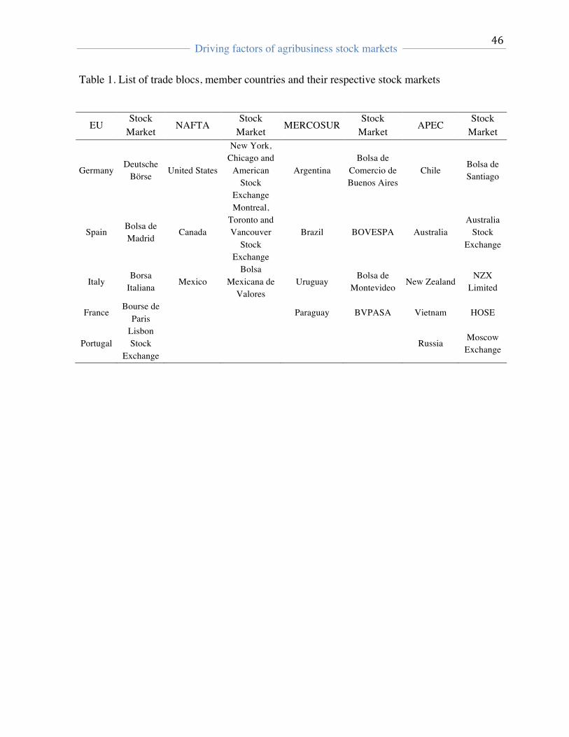
!
!
Driving factors of agribusiness stock markets
!! !
46!
Table 1. List of trade blocs, member countries and their respective stock markets
EU Stock
Market NAFTA Stock
Market MERCOSUR Stock
Market APEC Stock
Market
Germany Deutsche
Börse United States
New York, Chicago and
American Stock
Exchange
Argentina Bolsa de
Comercio de Buenos Aires
Chile Bolsa de Santiago
Spain Bolsa de Madrid
Canada
Montreal, Toronto and Vancouver
Stock Exchange
Brazil BOVESPA Australia Australia
Stock Exchange
Italy Borsa
Italiana Mexico Bolsa
Mexicana de Valores
Uruguay Bolsa de
Montevideo New Zealand NZX
Limited
France Bourse de
Paris Paraguay BVPASA Vietnam HOSE
Portugal Lisbon Stock
Exchange
Russia Moscow Exchange
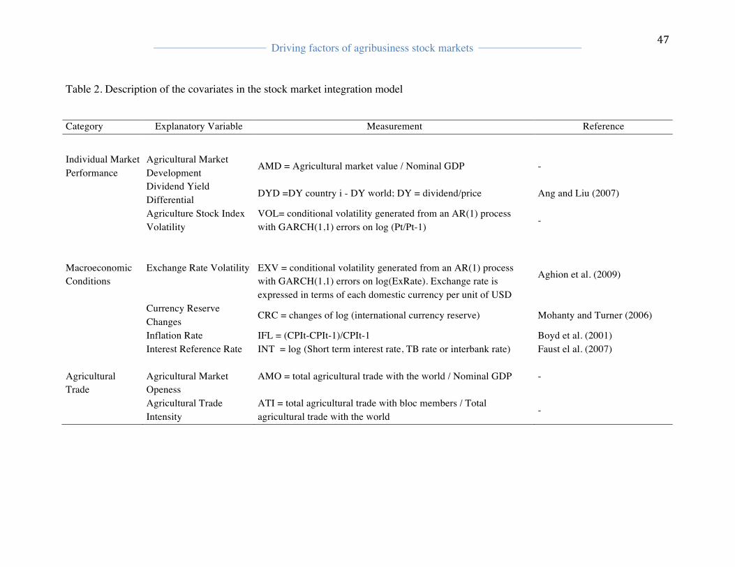
!
!
Driving factors of agribusiness stock markets
!! !
47!
Table 2. Description of the covariates in the stock market integration model
Category Explanatory Variable Measurement Reference
Individual Market Performance
Agricultural Market Development
AMD = Agricultural market value / Nominal GDP -
Dividend Yield Differential DYD =DY country i - DY world; DY = dividend/price Ang and Liu (2007)
Agriculture Stock Index Volatility
VOL= conditional volatility generated from an AR(1) process with GARCH(1,1) errors on log (Pt/Pt-1) -
Macroeconomic Conditions
Exchange Rate Volatility
EXV = conditional volatility generated from an AR(1) process with GARCH(1,1) errors on log(ExRate). Exchange rate is expressed in terms of each domestic currency per unit of USD
Aghion et al. (2009)
Currency Reserve Changes CRC = changes of log (international currency reserve) Mohanty and Turner (2006)
Inflation Rate IFL = (CPIt-CPIt-1)/CPIt-1 Boyd et al. (2001) Interest Reference Rate INT = log (Short term interest rate, TB rate or interbank rate) Faust el al. (2007) Agricultural Trade
Agricultural Market Openess
AMO = total agricultural trade with the world / Nominal GDP -
Agricultural Trade Intensity
ATI = total agricultural trade with bloc members / Total agricultural trade with the world -
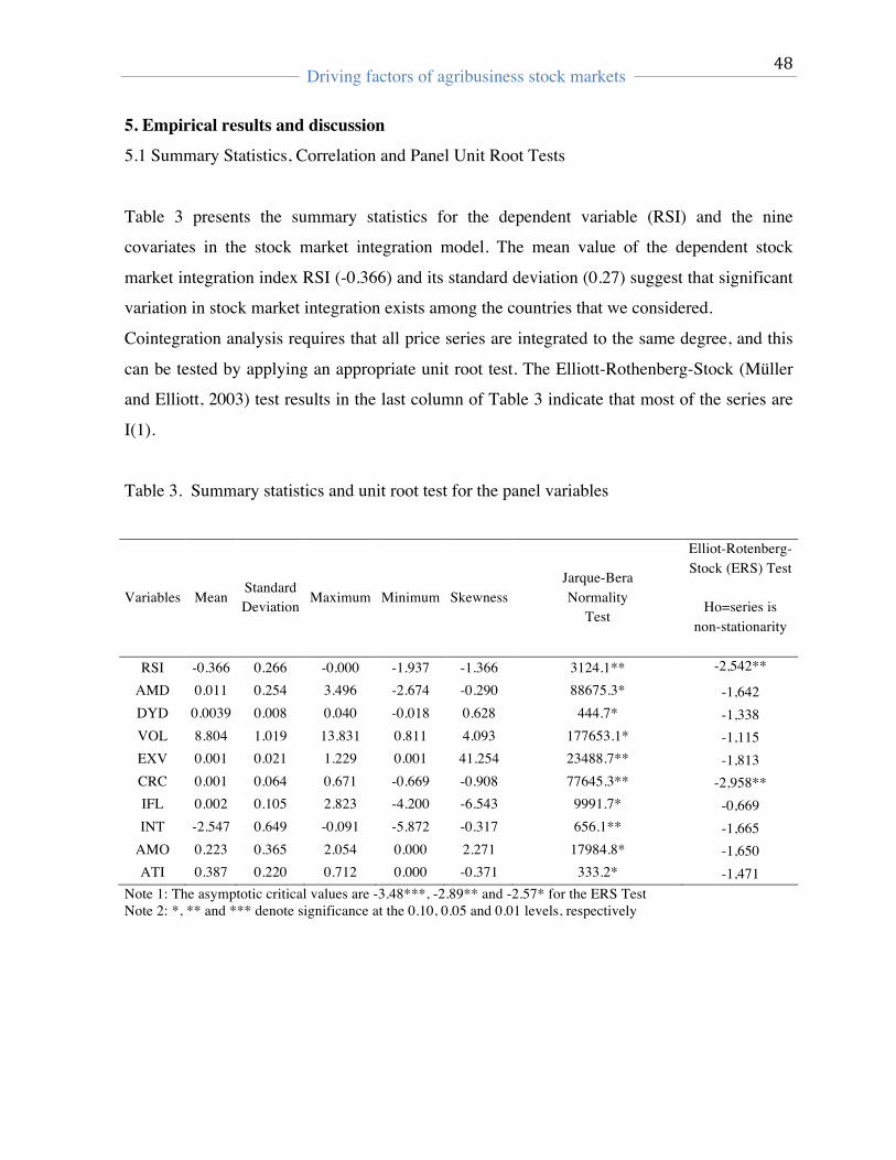
! Driving factors of agribusiness stock markets
!! !
48!
!
5. Empirical results and discussion
5.1 Summary Statistics, Correlation and Panel Unit Root Tests
Table 3 presents the summary statistics for the dependent variable (RSI) and the nine
covariates in the stock market integration model. The mean value of the dependent stock
market integration index RSI (-0.366) and its standard deviation (0.27) suggest that significant
variation in stock market integration exists among the countries that we considered.
Cointegration analysis requires that all price series are integrated to the same degree, and this
can be tested by applying an appropriate unit root test. The Elliott-Rothenberg-Stock (Müller
and Elliott, 2003) test results in the last column of Table 3 indicate that most of the series are
I(1).
Table 3. Summary statistics and unit root test for the panel variables
Variables Mean Standard Deviation Maximum Minimum Skewness
Jarque-Bera Normality
Test
Elliot-Rotenberg-Stock (ERS) Test
Ho=series is
non-stationarity
RSI -0.366 0.266 -0.000 -1.937 -1.366 3124.1** -2,542** AMD 0.011 0.254 3.496 -2.674 -0.290 88675.3* -1,642 DYD 0.0039 0.008 0.040 -0.018 0.628 444.7* -1,338 VOL 8.804 1.019 13.831 0.811 4.093 177653.1* -1,115 EXV 0.001 0.021 1.229 0.001 41.254 23488.7** -1,813 CRC 0.001 0.064 0.671 -0.669 -0.908 77645.3** -2,958** IFL 0.002 0.105 2.823 -4.200 -6.543 9991.7* -0,669 INT -2.547 0.649 -0.091 -5.872 -0.317 656.1** -1,665
AMO 0.223 0.365 2.054 0.000 2.271 17984.8* -1,650 ATI 0.387 0.220 0.712 0.000 -0.371 333.2* -1,471
Note 1: The asymptotic critical values are -3.48***, -2.89** and -2.57* for the ERS Test Note 2: *, ** and *** denote significance at the 0.10, 0.05 and 0.01 levels, respectively
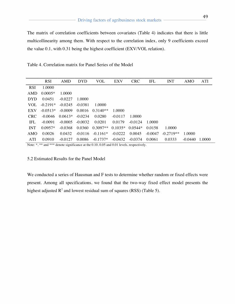
! Driving factors of agribusiness stock markets
!! !
49!
!
The matrix of correlation coefficients between covariates (Table 4) indicates that there is little
multicollinearity among them. With respect to the correlation index, only 9 coefficients exceed
the value 0.1, with 0.31 being the highest coefficient (EXV/VOL relation).
Table 4. Correlation matrix for Panel Series of the Model
RSI AMD DYD VOL EXV CRC IFL INT AMO ATI RSI 1.0000
AMD 0.0005* 1.0000 DYD 0.0451 -0.0227 1.0000
VOL -0.2191* -0.0245 -0.0381 1.0000 EXV -0.0513* -0.0009 0.0016 0.3140** 1.0000
CRC -0.0046 0.0613* -0.0234 0.0280 -0.0117 1.0000 IFL -0.0091 -0.0005 -0.0032 0.0201 0.0179 -0.0124 1.0000
INT 0.0957* -0.0368 0.0360 0.3097** 0.1035* 0.0544* 0.0158 1.0000
AMO 0.0026 0.0432 -0.0116 -0.1161* -0.0222 0.0045 -0.0047 -0.2719** 1.0000
ATI 0.0910 -0.0127 0.0086 -0.1737* -0.0432 -0.0374 0.0061 0.0333 -0.0440 1.0000 Note: *, ** and *** denote significance at the 0.10, 0.05 and 0.01 levels, respectively.
5.2 Estimated Results for the Panel Model
We conducted a series of Hausman and F tests to determine whether random or fixed effects were
present. Among all specifications, we found that the two-way fixed effect model presents the
highest adjusted R2 and lowest residual sum of squares (RSS) (Table 5).
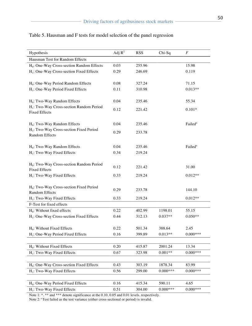
! Driving factors of agribusiness stock markets
!! !
50!
!
Table 5. Hausman and F tests for model selection of the panel regression
Hypothesis Adj R2 RSS Chi-Sq F Hausman Test for Random Effects H0: One-Way Cross-section Random Effects 0.03 255.96 15.98 H1: One-Way Cross-section Fixed Effects 0.29 246.69 0.119 H0: One-Way Period Random Effects 0.08 327.24 71.15 H1: One-Way Period Fixed Effects 0.11 310.98 0.013** H0: Two-Way Random Effects 0.04 235.46 55.34 H1: Two-Way Cross-section Random Period Fixed Effects
0.12 221.42 0.101*
H0: Two-Way Random Effects 0.04 235.46 Faileda H1: Two-Way Cross-section Fixed Period Random Effects
0.29 233.78
H0: Two-Way Random Effects 0.04 235.46 Faileda H1: Two-Way Fixed Effects 0.34 219.24 H0: Two-Way Cross-section Random Period Fixed Effects 0.12 221.42 31.00
H1: Two-Way Fixed Effects 0.33 219.24 0.012** H0: Two-Way Cross-section Fixed Period Random Effects
0.29 233.78 144.10
H1: Two-Way Fixed Effects 0.33 219.24 0.012** F-Test for fixed effects H0: Without fixed effects 0.22 402.99 1198.01 55.15 H1: One-Way Cross-section Fixed Effects 0.44 312.13 0.037** 0.050** H0: Without Fixed Effects 0.22 501.34 388.64 2.45 H1: One-Way Period Fixed Effects 0.16 399.89 0.013** 0.000*** H0: Without Fixed Effects 0.20 415.87 2001.24 13.34 H1: Two-Way Fixed Effects 0.67 323.98 0.001** 0.000*** H0: One-Way Cross-section Fixed Effects 0.43 303.19 1878.34 83.99 H1: Two-Way Fixed Effects 0.56 299.00 0.000*** 0.000*** H0: One-Way Period Fixed Effects 0.16 415.34 590.11 4.65 H1: Two-Way Fixed Effects 0.51 304.00 0.000*** 0.000*** Note 1: *, ** and *** denote significance at the 0.10, 0.05 and 0.01 levels, respectively. Note 2: a Test failed as the test variance (either cross-sectional or period) is invalid.
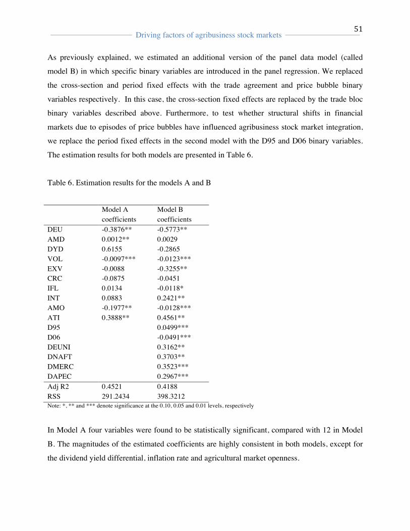
! Driving factors of agribusiness stock markets
!! !
51!
!
As previously explained, we estimated an additional version of the panel data model (called
model B) in which specific binary variables are introduced in the panel regression. We replaced
the cross-section and period fixed effects with the trade agreement and price bubble binary
variables respectively. In this case, the cross-section fixed effects are replaced by the trade bloc
binary variables described above. Furthermore, to test whether structural shifts in financial
markets due to episodes of price bubbles have influenced agribusiness stock market integration,
we replace the period fixed effects in the second model with the D95 and D06 binary variables.
The estimation results for both models are presented in Table 6.
Table 6. Estimation results for the models A and B
Model A coefficients
Model B coefficients
DEU -0.3876** -0.5773** AMD 0.0012** 0.0029 DYD 0.6155 -0.2865 VOL -0.0097*** -0.0123*** EXV -0.0088 -0.3255** CRC -0.0875 -0.0451 IFL 0.0134 -0.0118* INT 0.0883 0.2421** AMO -0.1977** -0.0128*** ATI 0.3888** 0.4561** D95 0.0499*** D06 -0.0491*** DEUNI 0.3162** DNAFT 0.3703** DMERC 0.3523*** DAPEC 0.2967*** Adj R2 0.4521 0.4188 RSS 291.2434 398.3212 Note: *, ** and *** denote significance at the 0.10, 0.05 and 0.01 levels, respectively
In Model A four variables were found to be statistically significant, compared with 12 in Model
B. The magnitudes of the estimated coefficients are highly consistent in both models, except for
the dividend yield differential, inflation rate and agricultural market openness.
! Driving factors of agribusiness stock markets
!! !
52!
!
5.2.1 Individual market performance category
In both models we found a positive relationship between RSI and the size of the agribusiness
sector as a percentage of total GDP (AMD). This result suggests that increased capitalization of
agribusiness firms as a percentage of GDP stabilizes the firm’s valuation. The previous statement
confirms the notion that high sector growth expectations would promote market integration via
greater financial stability. In emerging markets, the relationship between sector GDP growth and
stock valuation has been demonstrated previously by the work of Pendell and Cho (2013).
The market volatility coefficients (VOL) are (-) 0.0097 for model A and (-) 0.0123 for model B,
suggesting that this has a negative effect on the integration process between stock markets.
Increased levels of volatility do not promote regional stock market integration because this
mainly depend of the development level of each stock market, and is driven by a different
economic process than pricing returns (Bekaert and Harvey, 1997). In fact, Esqueda et al. (2013)
demonstrated that the correlation between local and global market returns increases as a result of
market-oriented policies, but these policies do not drive up local market volatility. In both
models, DVD shows statistically significant coefficients, but in different directions (positive in
model A and negative in model B). This impedes us from being able to make conclusions
regarding a single effect of this variable on RSI.
Certainly, the aforementioned results confirm that countries can benefit from trade regionalism
policies in terms of stock return pricing, by acting as an economic bloc rather than as individual
markets. The main consequence of such policies is an increase in market options and stability as
a result of higher capitalization levels.
5.2.2 Macroeconomic conditions category
This category includes macroeconomic and stability indicators, namely: exchange rate volatility
(EXV), inflation rate (IFL), interest reference rate (INT) and currency reserves changes (CRC).
As expected, EXV has a significant and negative effect on agribusiness stock market integration
in both models (-0.088 and -0.3255 for model A and B respectively), confirming an inverse
relationship with respect to stock market integration. According to Gounopoulos et al. (2013),
unexpected changes in currency values affects price convergence among stock markets because
of their effect on macroeconomic stability and economic expectations. Both coefficients are high
! Driving factors of agribusiness stock markets
!! !
53!
!
in absolute value, suggesting that this variable has an important impact as driving factor of
regional stock markets. Because it affects the economy’s ability to finance international trade, the
large-scale use of currency reserves has significant macroeconomic implications. In fact, our
model’s coefficients show an inverse relationship between changes in currency reserves (CRC)
and stock market integration. Changes in currency reserves are often associated with exchange
rate changes that increase the risks of holding instruments. This has a positive relationship with
the risk exposures of stock instruments due to the use of foreign exchange reserves to resist
currency appreciation, which has been demonstrated previously by Mohanty and Turner (2006).
INF has a negative coefficient in both models, but only in model B is it statistically significant.
Bittencurt (2011) finds an inverse relationship between inflation and stock market integration
because high inflation levels intensify financial market frictions and reduce the efficiency of the
financial system. Moreover, our results are in line with those of De Grauwe (2012) who
demonstrated that high inflation rates dampen the attraction of capital flows, further decreasing
arbitrage activities between stock markets. Interest rates represent the return on alternative assets
to stocks, and the discount rates used on stock return valuations. In models A and B, INT is
positively correlated with market integration, recording values of 0.09 and 0.24 respectively.
Ehrmann and Fratzscher (2011) conclude that higher interest rates increase stock market
integration because they divert capital from the stock market to the bond market. With the
increasing ease of market access as a result of trade agreements, regional stock investments are
promoted because higher bond returns attract local investors to introduce their capital into
regional markets.
5.2.3 Agricultural trade category
The trade indicators used were agricultural market openness (AMO) and agricultural trade
intensity (ATI). As expected, agricultural trade intensity (ATI), which measures total agricultural
trade with block members as a proportion of total agricultural trade with the world, unlike
agricultural market openness (AMO) which measures agricultural trade with the world as a
proportion of nominal GDP, is positive and significant in both models. While the ATI values
were 0.3888 for model A and 0.4561 for model B, the AMO coefficient was -0.1977 and -
0.01288 respectively.
! Driving factors of agribusiness stock markets
!! !
54!
!
ATI has a positive relationship with RSI because the higher the trade flow between regional bloc
members, the higher the level of regional stock market integration. This implies that higher levels
of market access and trade due to regional liberalization policies promote stock market
integration and thus capital flows between countries or sectors, further supporting the hypothesis
of this work.
Although previous studies on developed countries (Aghion et al., 2009 and De Grauwe, 2012)
suggested that volatility and/or risk are important factors in the behavior of stock markets, our
results demonstrate that for the agribusiness sector the effect of this type of determinant variable
is not so significant. This could benefit emerging countries or developing markets that usually
present higher risk qualifications. Overall, we confirm the relevance of the agribusiness sector
within the country, and economic blocs are key driving factors of stock market integration. These
results constitute a novel contribution to the literature, as most studies have not considered
sectorial characteristics, production and trade among the factors that promote the integration of
stock markets.
5.2.4 Price bubbles and Trade blocs
Price bubbles are driving factors of market integration because of their effects on price
differences and consequently arbitrage activities (Gilbert, 2010). In our model, all price bubble
variables present statistically significant coefficients. This result supports the existence of two-
way fixed effects. Among these, the first period dummy (D95) had a positive and significant
effect on market integration with an estimated coefficient of 0.0499. However, the second period
(D06) had a negative effect of - 0.0491. The higher impact on market integration from the D95
bubble could be a consequence of the increased arbitrage activities among commodity traders
when compared to 2006 bubble because of the higher domestic/international price spread during
1995 bubble when compared to 2006 (Gilbert, 2010; Esposti and Listorti, 2013). The D95 bubble
had the effect of increasing stock prices and as such return pricing behavior for agribusiness
stocks. In other words, the greater price spread during the 1995 crisis seems to have promoted
arbitrage activities among regional investors who held agribusiness stocks from markets with
lower commodity prices to markets with higher commodity prices.
The last group of variables included in model B is the presence of regional trade agreements
pertaining to each of the countries considered in this work. For both models, they present positive
! Driving factors of agribusiness stock markets
!! !
55!
!
and statistically significant coefficients. Our findings provide a clear picture of the positive effect
of the implementation of trade agreements on regional market integration, further confirming
previous results (Gochoco-Bautista and Remolona, 2012; Caporale and Spagnolo, 2012). The
impact on market integration is relatively homogeneous for all agreements, suggesting that
regardless of the level the economic development of each country and stock market price
arbitrage among different markets, the benefit in all blocs is present to a similar degree.
The highest degree of integration is found in a developed market, NAFTA, followed by
MERCOSUR, EU and APEC. In the case of NAFTA and MERCOSUR, factors such as distance
and public policies could drive a greater degree of market integration. This argument is supported
by Lahrech and Sylwester (2013), who find a positive relationship between the integration of
financial markets and the distance between them. However, our results for the EU - where the
markets considered in Germany, Italy, France, Portugal and Spain are geographically closer to
one another than the markets in, for example NAFTA - are more similar to those of Bekaert et al.
(2011). Their results demonstrate an inverse relationship between the number of stock markets
and the degree of pricing efficiency when a large number of stock markets are analyzed. Bekaert
et al. (2011) suggest that financial provisions policies to reduce transaction costs for capital flows
can promote greater integration in regional risk pricing. Recently, both blocks have generated
legal initiatives with the aim of fulfilling this objective and promoting capital flows between their
member countries.
Furthermore, the heterogeneity of the members of an RTA might play a more important role than
geographic distance between them. For example, in the case of APEC the differences between
their stock markets in terms of trade volume, the distance (for example, between Chile and
Russia) and the competitive trade policies among them could work against effective cooperation
between countries. The negative effect of these policies on capital flows and financial
cooperation has been demonstrated previously in the works of Click and Plummer (2005) and
Karim and Ning (2013).
Overall, our findings suggest that trade blocs as well as price bubbles play a relevant role in
arbitrage activities between stock markets. Moreover, market stability indicators (i.e. AMD
and/or VOL) have more explanatory power than performance level, such as for example DYD, as
drivers of regional stock market integration. The integration of stock markets is more exposed to
individual and regional market stability than world level conditions. Finally, the empirical
! Driving factors of agribusiness stock markets
!! !
56!
!
evidence documented here demonstrates that market stability is a significant factor for
convergence in regional risk pricing on stock markets.
6. Conclusion
The recent trend towards economic regionalism and its effect on the agricultural sector has
become a catalyst for research on the stock dynamics of agribusiness firms. This work aimed to
explore the drivers of regional stock market integration with a focus on the agribusiness sector
across the most important trade blocs around the world. This was a previously unexplored issue
in the literature on stock market integration.
In this study, a regional integration framework, which combines information from three
categories and nine explanatory variables, is used to examine the contributing factors to regional
stock market integration. We also consider agriculture-specific factors to control for possible
structural breaks and trade agreement effects.
We conclude that our categories have been important factors in promoting regional stock market
integration, further suggesting that this process is driven by the market performance,
macroeconomic conditions and agricultural trade of each country. Among them, market stability
indicators and intra-regional trade levels have greater explanatory power than performance
variables as drivers of regional stock market integration. Besides this, the integration of stock
markets is more exposed to individual and regional market stability than world level conditions
(for example ATI vs AMO). Furthermore, stock market integration was strengthened by the
implementation of trade agreements and during the 1995 price bubble.
The level of market integration differs according the number of countries participating in the each
stock market. The integration level is higher for small trade blocs (in terms of countries), such as
for example NAFTA and MERCOSUR, when compared with a more segmented bloc such as the
EU or APEC. Our results suggest that the level of development and public policies also play a
role in the integration pattern of each regional market.
Acknowledgements
The authors acknowledge financial support for this research from the Chilean Commission for
Scientific and Technological Research (CONICYT)-Folio No. 21120286.
! Driving factors of agribusiness stock markets
!! !
57!
!
7. References
Aghion, P., Bacchetta, P., Ranciere, R., and Rogoff, K., 2009. Exchange rate volatility and
productivity growth: the role of financial development. Journal of Monetary Economics 56, 494-
513.
Ang, A. and Liu, J., 2007. Risk, return, and dividends. Journal of Financial Economics 85, 1-38.
Bekaert, G., Harvey, C.R. and Lumsdaine, R.L. 2002. Dating the integration of world equity
markets. Journal of Financial Economics 65, 203-247.
Bekaert, G., Harvey, C. R., and Lundblad, C., 2011. Financial openness and productivity. World
Development 39, 1-19.
Berman, N., and Héricourt, J. 2010., Financial factors and the margins of trade: Evidence from
cross-country firm-level data. Journal of Development Economics 93, 206-217.
Bittencourt, M. 2011., Inflation and financial development: Evidence from Brazil. Economic
Modelling 28, 91-99.
Borenstein, S. and Farrell, J. 2007., Do investors forecast fat firms? Evidence from the
gold‐mining industry. The RAND Journal of Economics 38, 626-647.
Boyd, J., Levine, R. and Smith, B. 2001., The impact of inflation on financial sector
performance. Journal of Monetary Economics 47, 221-248.
Caporale, G. and Spagnolo, N. 2012., Stock market integration between three CEECs. Journal of
Economic Integration 27, 115-122.
Carneiro, J. and Brenes, T. 2014., Latin American firms competing in the global economy.
Journal of Business Research 67, 831–836
Carrieri, F., Errunza, V.R. and Hogan, K. 2007., Characterizing world market integration through
time. Journal of Financial and Quantitative Analysis 42, 915-940.
Casu, B., and Girardone, C. 2010., Integration and efficiency convergence in EU banking
markets. Omega 38, 260-267.
Chami, R., Fullenkamp, C. and Sharma, S. 2010., A framework for financial market
development. Journal of Economic Policy Reform 13, 107-135.
Click, R. and Plummer, M. 2005., Stock market integration in ASEAN after the Asian financial
crisis. Journal of Asian Economics 16, 5-28.
De Grauwe, P. 2012., Lessons from the Eurocrisis for East Asian Monetary Relations. World
Economy 35, 405–418.
! Driving factors of agribusiness stock markets
!! !
58!
!
Diamandis, P. and Drakos, A. 2011., Financial liberalization, exchange rates and stock prices:
exogenous shocks in four Latin America countries. Journal of Policy Modeling, 33, 381-394.
Dieter, H. 2003., Exploring alternative theories of economic regionalism: from trade to finance in
Asian co-operation?. Review of International Political Economy 10, 430-454.
Dufour, J., Khalaf, L., and Beaulieu, M. 2010., Multivariate residual‐based finite‐sample tests for
serial dependence and ARCH effects with applications to asset pricing models. Journal of
Applied Econometrics 25, 263-285.
Ehrmann, M., Fratzscher, M., and Rigobon, R. 2011., Stocks, bonds, money markets and
exchange rates: measuring international financial transmission. Journal of Applied Econometrics
26, 948-974.
Esqueda, O. A., Luo, Y. and Jackson, D. O. 2013.,The linkage between the US “fear index” and
ADR premiums under non-frictionless stock markets. Journal of Economics and Finance 22, 1-
16.
Esposti, R. and Listorti, G. 2013., Agricultural price transmission across space and commodities
during price bubbles. Agricultural Economics 44, 125-139.
Fama, E. F. and French, K. R. 2012., Size, value, and momentum in international stock returns.
Journal of Financial Economics 105, 457-472.
FAOSTAT, 2014., Statistics, Agricultural Trade, Internet Database. http://www.fao.org/faostat .
Faust, J., Rogers, J. H., Wang, S. Y. B., & Wright, J. H., 2007. The high-frequency response of
exchange rates and interest rates to macroeconomic announcements. Journal of Monetary
Economics 54, 1051-1068.
Gilbert, C. L. 2010., How to understand high food prices. Journal of Agricultural Economics 61,
398-425.
Glezakos, M., Merika, A. and Kaligosfiris, H. 2007., Interdependence of major world stock
exchanges: How is the Athens stock exchange affected. International Research Journal of Finance
and Economics 7, 24-39.
Gochoco-Bautista, M. and Remolona, E. 2012., Going Regional: How to Deepen ASEAN’s
Financial Markets. Asian Development Bank Economics Working Paper Series No. 300.
Available at SSRN: http://ssrn.com/abstract=2032824
Gounopoulos, D., Molyneux, P., Staikouras, S. K., Wilson, J. O., and Zhao, G. 2013., Exchange
rate risk and the equity performance of financial intermediaries. International Review of
Financial Analysis 29, 271-282.
! Driving factors of agribusiness stock markets
!! !
59!
!
Grullon, G., Lyandres, E. and Zhdanov, A. 2012., Real Options, Volatility, and Stock Returns.
The Journal of Finance, 67: 1499–1537.
Guangxi, C., Yan, H., and Weijun, C. 2014., Time-varying long memories of the chinese
currency and stock markets based on the hurst exponent. Fluctuation and noise letters 13, 12:21.
Guvenen, F. 2009., A parsimonious macroeconomic model for asset pricing. Econometrica 77,
1711-1750.
Hausman, J.A. 1978., Specification Tests in Econometrics. Econometrica, 46 (6), 1251–1271
Heaney, R., Hooper, V. and Jaugietis, M. 2002., Regional Integration of Stock Markets in Latin
America. Journal of Economic Integration, 17: 745-760.
Lahrech, A. and Sylwester, K. 2013., The impact of NAFTA on North American stock market
linkages. The North American Journal of Economics and Finance 25, 94-108.
Herrmann, S. and Mihaljek, D. 2013., The determinants of cross‐border bank flows to emerging
markets. Economics of Transition 21, 479-508.
Hilscher, J. and Raviv, A. 2011., Bank stability and market discipline: The effect of contingent
capital on risk taking and default probability. Brandeis University, Massachusetts.
Hooper, V. and Jaugietis, M. 2000., The impact of liberalization and regionalism upon capital
markets in emerging Asian economies. International Finance Review 1: 219-255.
Hooy, C. W. and Goh, K. L. 2008., International asset pricing models: The case of ASEAN stock
markets. International Journal of Banking and Finance 6, 7-15.
Jawadi, F., El Hedi Arouri, M., and Bellalah, M. 2010., Nonlinear Linkages between Oil and
Stock Markets in Developed and Emerging Countries. International Journal of Business,15, 22-
31.
Karim, B. and Ning, H. 2013., Driving forces of the ASEAN-5 stock markets integration, Asia-
Pacific Journal of Business Administration 5,186:191
Karim, B., Mohamadm, J. and Karim, S. 2011., The subprime crisis and stock index futures
markets integration, Journal of Risk Finance 12, 400:408.
Kose, M., Prasad, E. and Terrones, M. 2006., How do trade and financial integration affect the
relationship between growth and volatility?. Journal of international Economics, 69(1), 176-202.
Levine, R. and Zervos, S. 1998., Stock markets, banks, and economic growth. American
Economic Review, 88: 537-558.
Mohanty, S. and Turner, P. 2006., Intervention: what are the domestic consequences?. BIS
Quarterly Review 29: 39-52.
! Driving factors of agribusiness stock markets
!! !
60!
!
Müller, U. K. and Elliott, G. 2003., Tests for unit roots and the initial condition. Econometrica,
71(4), 1269-1286.
Nagel, S. and Singleton, K. J. 2011., Estimation and evaluation of conditional asset pricing
models. The Journal of Finance 66, 873-909.
Nguyen, C. and Bhatti, M. 2012., Copula model dependency between oil prices and stock
markets: Evidence from China and Vietnam. Journal of International Financial Markets,
Institutions and Money 22, 758-773.
Pendell, D. L. and Cho, C. 2013., Stock Market Reactions to Contagious Animal Disease
Outbreaks: An Event Study in Korean Foot-and-Mouth Disease Outbreaks. Agribusiness
29, 455–468.
Oskooe, S., Li, H., and Shamsavari, A. 2010., The random walk hypothesis in emerging stock
market. International Research Journal of Finance and Economics 50, 51-61.
Sheng, L. 2014., Capital Controls and International Development: A Theoretical
Reconsideration. Global Policy 5, 114–120.
Tepe, F. S., Du, X. and Hennessy, D. A. 2011., The impact of biofuels policy on agribusiness
stock prices. Agribusiness 27, 179–192.
World Trade Organization.2013., International Trade Statistics 2013.<
http://www.wto.org/english/res_e/statis_e/its2013_e/its13_toc_e.htm>.
! Spatial market integration and fuel prices
!! !
61!
!
CHAPTER 5.
Spatial market integration and fuel prices: an empirical analysis of the Chilean
horticultural sector
Rodrigo Valdes a,b,*, Stephan Von Cramon-Taubadel a , Alejandra Engler b
a Georg-August-Universitat Gottingen, Department of Agricultural Economics and Rural
Development. Platz der Gottinger Sieben 5, 37073, Gottingen, Germany
b Universidad de Talca. Facultad de Ciencias Agrarias. Departamento de Economia Agraria.
Casilla 747-721, Talca, Chile.
*Corresponding Author. Universidad de Talca. Facultad de Ciencias Agrarias. Departamento de
Economia Agraria. Casilla 747-721, Talca, Chile.
Email: [email protected]
! Spatial market integration and fuel prices
!! !
62!
!
ABSTRACT
The role played by the fuel prices on the price transmission between central and regional
horticultural markets has been an unexplored field of research on developing countries.
The aim of this article is to a propose a procedure to estimate a regime-dependent vector error
correction model with an exogenous threshold variable (Chilean retail fuel prices) were not only
the short and long- run equilibrium relationship itself can display threshold-type non-linearity.
The proposed approach is unique in explicitly testing the threshold cointegration process based
on the Gonzalo and Pitarakis (2006) test. We considered the most relevant central and regional
wholesale markets (Santiago and Talca) the prices of the most planted Chilean horticultural
products, namely: maize, tomato, onion, carrot. In order to account for the fuel prices, we
consider the Chilean retail prices. The reserach was conducted using a price series of weekly
frequency for the period January 2009 to December 2013. We identify two price transmission
regimes characterized by different equilibrium relationships and short-run adjustment processes.
For mostly products, our empirical results confirms an unidirectional price transmission process
from central to regional markets which confirms a symmetric price adjustment and emphasized
the role of fuel prices on the price and speed of adjustements transmission elasticity. The results
imply that formation of the wholesale prices in both of the analyzed markets tend to be product
specific. The method proposed by this work appers to be is particularly suitable for capturing
irregular seasonal threshold effects in price transmission which is typical for vegetables.
Keywords: Spatial price transmission, market integration, threshold cointegration
! Spatial market integration and fuel prices
!! !
63!
!
1. Introduction
Price is the primary mechanism by which various levels of the market are linked. The extent of
adjustment and speed with which shocks are transmitted among producer, wholesale, and retail
market prices is an important factor reflecting the actions of market participants at different
levels. TIn this sense, the transmission of changes in the producer price to changes in the
consumer price depends, however, greatly on the type of product. For example, products that are
perishable and undergo minimal processing such as vegetables, fruit, and fresh milk, are expected
to have a relatively quick price transmission mechanism. Markets that are not integrated may
convey inaccurate price information, leading to misguided policy decisions and a misallocation
of resources. Sexton et al., (1991) identified three reasons for a lack of market integration:
imperfect competition, different trade barriers and prohibitive transactions costs. Transaction
costs are composed of transport cost, variable costs, customs duties and unmeasurable costs.
Among them, the most relevant in terms of price formation for all traded agricultural products are
the transport costs that are highly dependent of fuel prices (Ejrnæs and Persson, 2000).
Transport costs loom large in Chilean markets, because the long distances between main
wholesale markets and transport infrastructure dependent primarily on trucks. The movement of
products between warehouse markets provides a straightforward observation! of large variations
in transport distance, given that many fruits and vegetables are produced domestically.
Horticultural products are particularly sensitive to changes in fuel price because of the need for
refrigeration during transport. As a result, given that these products undergoes minimal
processing and packaging, the most important component of transaction cost is likely to be fuel
used in transportation. The effect of fuel prices on transport cost is well-identified, fuel price
increases can drive up transport costs, which in turn afffect the price of agricultural products
(Eryigit and Karaman, 2011). Accordingly, the role played by fuel prices offers an appropiate
method to analyse the effect of transport cost on the spatial integration level between horticultural
wholesale markets. In fact, there is still no clear evidence on the effect of the fuel prices has on
the integration process of horticultural markets in Chile. Consequently, the objective of this paper
is to analyze the role played by this factor on the spatial market integration between the major
horticultural products historically traded between two representatives wholesale markets Santiago
(a central market) and Talca (a representative regional market).
! Spatial market integration and fuel prices
!! !
64!
!
The use of regime dependent models to capture transaction costs are diverse, for example,
Negassa and Myers (2007) use parity bounds model to analyse policy effects and spatial market
efficiency using threshold model. Bakucs et al. (2007) and Bruemmer at al. (2009) apply Markov
Switching Models to analyse horizontal integration of German and Hungarian wheat prices, and
wheat prices in Ukraine respectively. Moreover, Bakucs and Ferto (2008) use Hansen and Seo
(2002) threshold cointegration test and Threshold Vector Error Correction model to test regional
milk price integration in Hungary.
Applications of regime dependent models assume that prices are linked by a constant long-run
equilibrium relationship (see for example, Alam et al. 2012). In the horticultural sector this
assumption may not always be justifiable. Horticultural markets are characterized by a fixed-
proportion relationship among farm inputs, wholesale products, and final retail products, as well
as an inelastic short-run supply owing to perishability and the timing of growing seasons (Pingali
et. al 2005). In order to overcome this issue, in this paper we propose a three-step procedure to
estimate a regime-dependent vector error correction model (VECM). In this model, not only the
short-run adjustment process towards equilibrium, but also the long- run equilibrium relationship
itself can display threshold-type non-linearity, as a function of the size of a stationary
variable,that in our case is the fuel prices, with respect to a threshold value. The proposed
approach is unique in explicitly testing the null hypothesis of linear cointegration against the
alternative of threshold cointegration based on a test proposed by Gonzalo and Pitarakis (2006).
We hypothesized, that long-run price relationships between Santiago and Talca wholesale
horticultural markets may display different patterns depending on the fuel prices.
The article proceeds as follows: the next section review relevant literature on market integration.
Sections 3 and 4 describe the corresponding econometric methodology and data sources. Section
5 and 6 present the results and discussion, respectively. Lastly, section 7 gives a conclusion.
2. The spatial market integration
The magnitude of trade relationship between markets or regions implies the existence of some
kind of price coordination mechanism (Bakucs and Ferto 2014). Perfectly integrated markets are
usually assumed to be efficient as well. In this paper however, we analyze whether long-run price
relationships underlying trade relationships exist between two horticultural wholesale markets
! Spatial market integration and fuel prices
!! !
65!
!
(Santiago and Talca). Tomek and Robinson (2003), defines the two axioms of the regional price
differences theory:
1. The price difference in any two regions or markets involved in trade with each other equals the
transaction costs.
2. The price difference between any two regions or markets not involved in trade with each other
is smaller than the transaction costs.
Let’s consider, two spatially different markets, where the price of a given good in time t is P1t and
P2t respectively. The two markets are considered integrated, if the price on market 1 equals the
price on market 2 corrected with transport costs, Kt:
!P1t =P2t +Kt (1)
Accordingly, trade between the two markets occurs only if |P1t – P2t|> Kt. That means that the
arbitrage ensures that prices of the same good traded in spatially separate markets equalise or
converge.
Following the definition given by Barrett (2001), TCs between a market “i” and “j” are composed
of transport costs (fij), where distance is one of the most important factors in the how TCs are
formed; variable costs (vij) associated with rates, cargo insurance, contracts, financial expenses,
hedging, sanitary and phytosanitary barriers; customs duties (dij); and unmeasurable costs (wij),
such as opportunity cost, the cost of searching for information and risk premiums.
Fuel prices can affect agricultural sector through different channels, being the most important
their link through transport costs. Fuel price increases can drive up transport costs, which in turn
affect the prices of all traded agricultural products. Interest in how fuel prices may affect fruits
and vegetable prices spans several areas of policy- oriented economic research. For example,
questions abound as to why retail food prices have become considerably more volatile since 2006
(Tegene, 2009) and if fuel price rallies affects the welfare level of rural producers due their effect
on transaction cost (Dillon and Barrett, 2013)
Transport costs loom large in Chilean markets, because the long distances between main
wholesale markets and transport infrastructure dependent primarily on trucks. The movement of
produce between warehouse markets provides a straightforward observation! of large variations in
! Spatial market integration and fuel prices
!! !
66!
!
transport distance, given that many fruits and vegetables are both produced domestically and
imported. Fresh produce is particularly sensitive to changes in fuel price because of the need for
refrigeration during transport (Pede, 2005). As a result, given that fresh produce undergoes
minimal processing and packaging, the most important component of transaction cost is likely to
be fuel used in transportation.
Applications of regime dependent models of price transmission assume that prices are linked by a
constant long-run equilibrium relationship, while allowing for threshold or switching effects in
the short-run adjustment process towards this equilibrium (Gonzalo and Pitarakis, 2006). In the
horticultural sector this assumption may not always be justifiable. Horticultural markets are
characterized by a fixed-proportion relationship among farm inputs, wholesale products, and final
retail products, as well as an inelastic short-run supply owing to perishability and the timing of
growing seasons (Goetz and Von Cramon-Taubadel, 2008). In this context, the factors that might
contribute to dampen the transmission of price signals are: inadequate infrastructure,
transportation bottlenecks, lack of market information, information asymmetry, market power,
menu cost (Park et al. 2002). These kinds of factors are common in developing countries
agricultural markets such as Chile and pose serious challenges to policy makers. So, estimating
the threshold in the price adjustment from one market to another or from one level to another in
the supply chain should be a rule rather than an exception, especially in the context of
horticultural markets.
3. Methods
The method proposed by Gonzalo and Pitarakis (2006) will be used to test the linear
cointegration null against the threshold cointegration between markets of Santiago and Talca. As
required, we will use the Chilean fuel price series as exogenous threshold variable. In this
approach, the null hypothesis of linear cointegration are:
yt = β′xt + ut, (2)
against the alternative hypothesis of cointegration with threshold effects:
yt =β′xt +λ′xtI(q t−d >γ)+ut ; with xt = xt−1 + vt , (3)
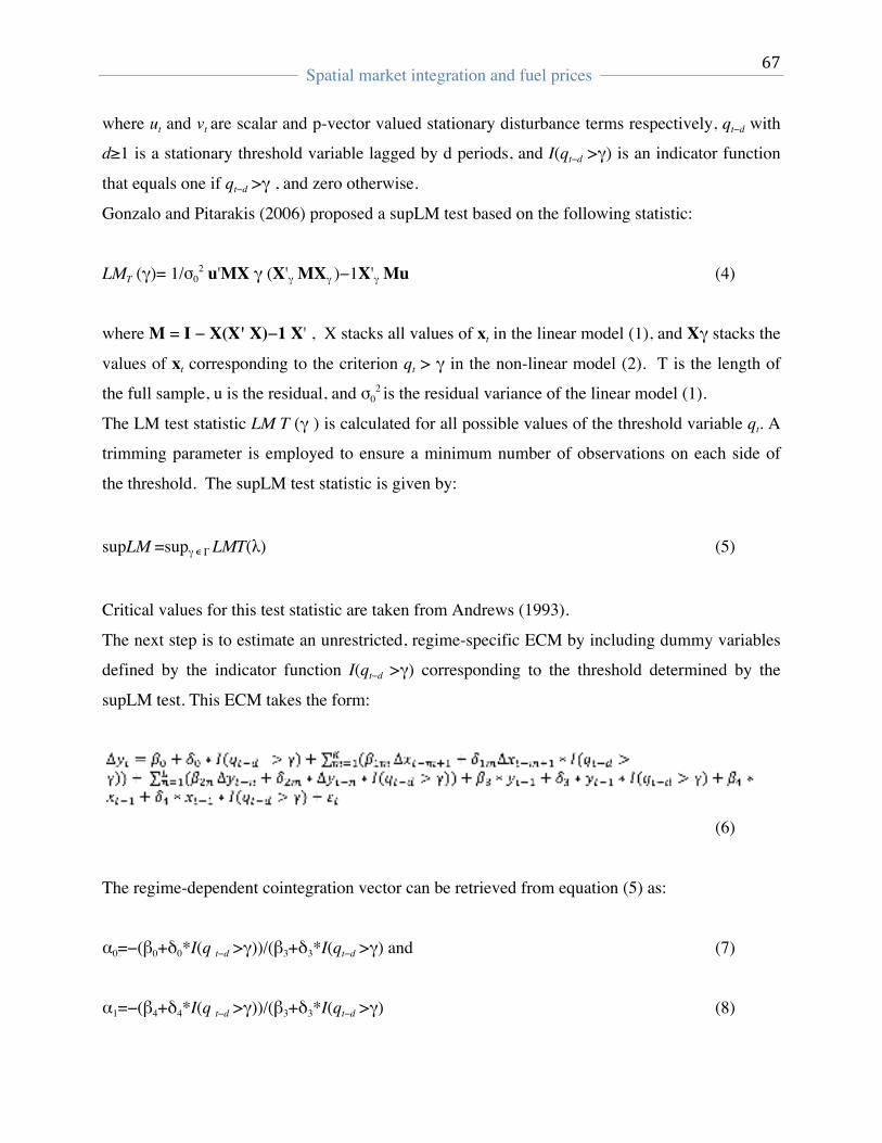
! Spatial market integration and fuel prices
!! !
67!
!
where ut and vt are scalar and p-vector valued stationary disturbance terms respectively, qt−d with
d≥1 is a stationary threshold variable lagged by d periods, and I(qt−d >γ) is an indicator function
that equals one if qt−d >γ , and zero otherwise.
Gonzalo and Pitarakis (2006) proposed a supLM test based on the following statistic:
LMT (γ)= 1/σ02 u'MX γ (X'γ MXγ )−1X'γ Mu (4)
where M = I − X(X' X)−1 X' , X stacks all values of xt in the linear model (1), and Xγ stacks the
values of xt corresponding to the criterion qt > γ in the non-linear model (2). T is the length of
the full sample, u is the residual, and σ02 is the residual variance of the linear model (1).
The LM test statistic LM T (γ ) is calculated for all possible values of the threshold variable qt. A
trimming parameter is employed to ensure a minimum number of observations on each side of
the threshold. The supLM test statistic is given by:
supLM =supγ�Γ LMT(λ) (5)
Critical values for this test statistic are taken from Andrews (1993).
The next step is to estimate an unrestricted, regime-specific ECM by including dummy variables
defined by the indicator function I(qt−d >γ) corresponding to the threshold determined by the
supLM test. This ECM takes the form:
(6)
The regime-dependent cointegration vector can be retrieved from equation (5) as:
α0=−(β0+δ0*I(q t−d >γ))/(β3+δ3*I(qt−d >γ) and (7)
α1=−(β4+δ4*I(q t−d >γ))/(β3+δ3*I(qt−d >γ) (8)
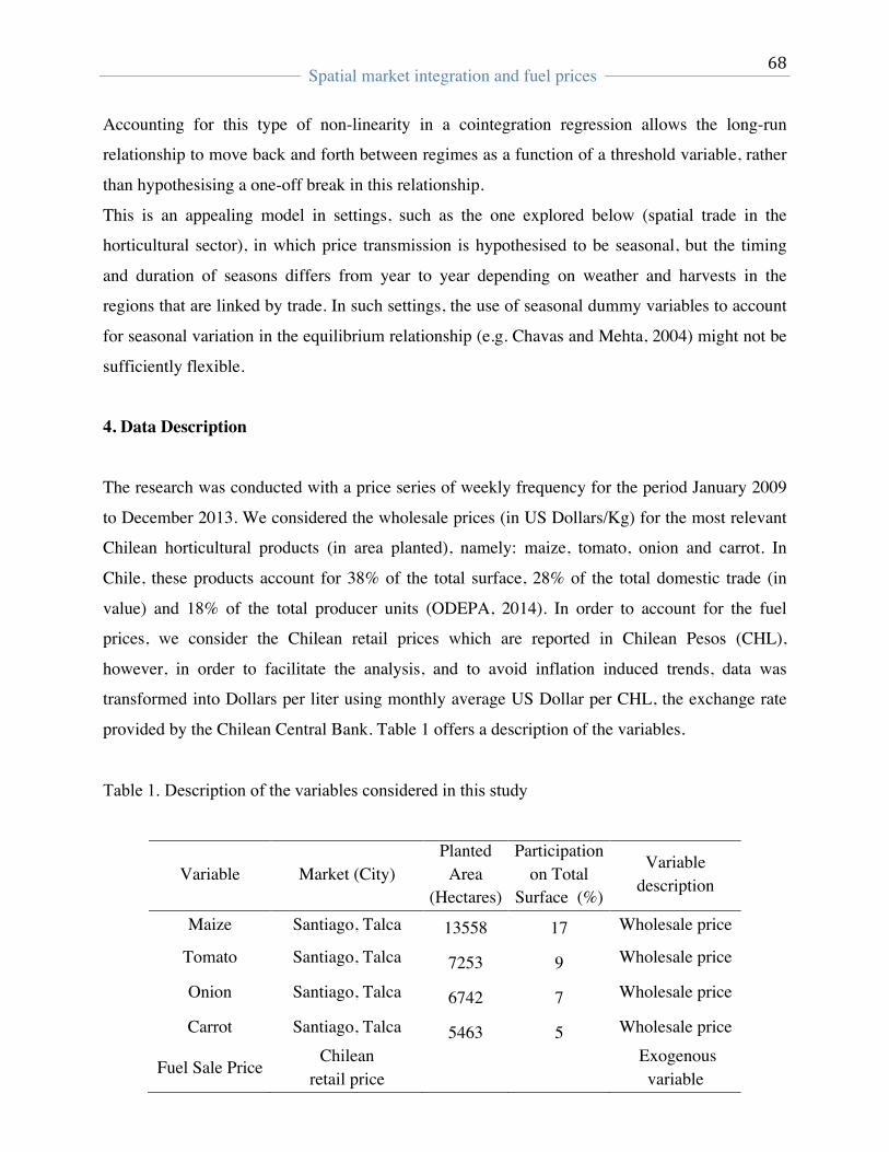
! Spatial market integration and fuel prices
!! !
68!
!
Accounting for this type of non-linearity in a cointegration regression allows the long-run
relationship to move back and forth between regimes as a function of a threshold variable, rather
than hypothesising a one-off break in this relationship.
This is an appealing model in settings, such as the one explored below (spatial trade in the
horticultural sector), in which price transmission is hypothesised to be seasonal, but the timing
and duration of seasons differs from year to year depending on weather and harvests in the
regions that are linked by trade. In such settings, the use of seasonal dummy variables to account
for seasonal variation in the equilibrium relationship (e.g. Chavas and Mehta, 2004) might not be
sufficiently flexible.
4. Data Description
The research was conducted with a price series of weekly frequency for the period January 2009
to December 2013. We considered the wholesale prices (in US Dollars/Kg) for the most relevant
Chilean horticultural products (in area planted), namely: maize, tomato, onion and carrot. In
Chile, these products account for 38% of the total surface, 28% of the total domestic trade (in
value) and 18% of the total producer units (ODEPA, 2014). In order to account for the fuel
prices, we consider the Chilean retail prices which are reported in Chilean Pesos (CHL),
however, in order to facilitate the analysis, and to avoid inflation induced trends, data was
transformed into Dollars per liter using monthly average US Dollar per CHL, the exchange rate
provided by the Chilean Central Bank. Table 1 offers a description of the variables.
Table 1. Description of the variables considered in this study
Variable Market (City) Planted
Area (Hectares)
Participation on Total
Surface (%)
Variable description
Maize Santiago, Talca 13558 17 Wholesale price
Tomato Santiago, Talca 7253 9 Wholesale price
Onion Santiago, Talca 6742 7 Wholesale price
Carrot Santiago, Talca 5463 5 Wholesale price
Fuel Sale Price Chilean
retail price
Exogenous variable
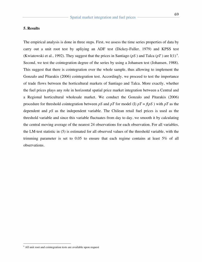
! Spatial market integration and fuel prices
!! !
69!
!
5. Results
The empirical analysis is done in three steps. First, we assess the time series properties of data by
carry out a unit root test by apliying an ADF test (Dickey-Fuller, 1979) and KPSS test
(Kwiatowski et al., 1992). They suggest that the prices in Santiago (pS ) and Talca (pT ) are I(1) 9.
Second, we test the cointegration degree of the series by using a Johansen test (Johansen, 1988).
This suggest that there is cointegration over the whole sample, thus allowing to implement the
Gonzalo and Pitarakis (2006) cointegration test. Accordingly, we proceed to test the importance
of trade flows between the horticultural markets of Santiago and Talca. More exactly, whether
the fuel prices plays any role in horizontal spatial price market integration between a Central and
a Regional horticultural wholesale market. We conduct the Gonzalo and Pitarakis (2006)
procedure for threshold cointegration between pS and pT for model (I) pT = f(pS ) with pT as the
dependent and pS as the independent variable. The Chilean retail fuel prices is used as the
threshold variable and since this variable fluctuates from day to day, we smooth it by calculating
the central moving average of the nearest 24 observations for each observation. For all variables,
the LM-test statistic in (5) is estimated for all observed values of the threshold variable, with the
trimming parameter is set to 0.05 to ensure that each regime contains at least 5% of all
observations.
9 All unit root and cointegration tests are available upon request
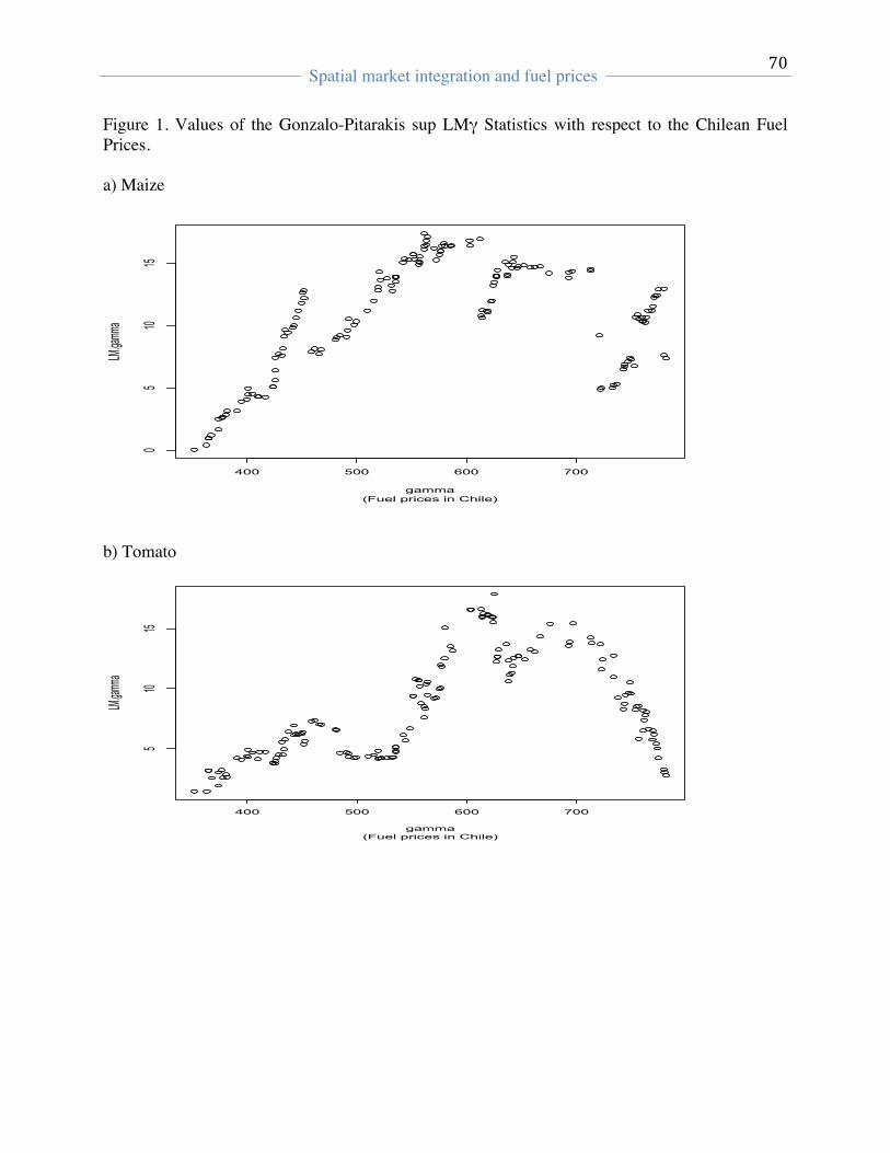
! Spatial market integration and fuel prices
!! !
70!
!
Figure 1. Values of the Gonzalo-Pitarakis sup LMγ Statistics with respect to the Chilean Fuel Prices. a) Maize
400 500 600 700
05
1015
Rm price (indep. var.)-Regional price (depend. var.)
(Fuel prices in Chile)gamma
LM.gamm
a
b) Tomato
400 500 600 700
510
15
Rm price (indep. var.)-Regional price (depend. var.)
(Fuel prices in Chile)gamma
LM.gam
ma
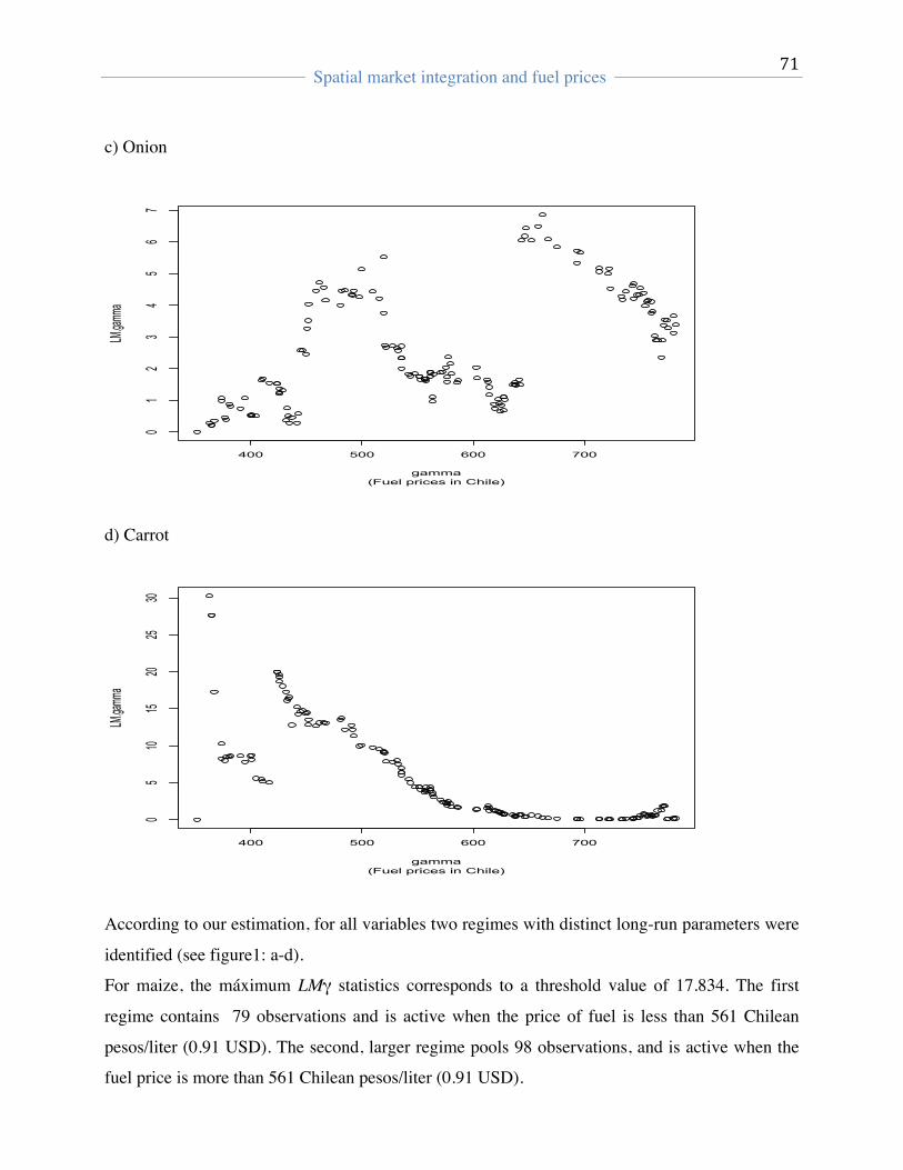
! Spatial market integration and fuel prices
!! !
71!
!
c) Onion
400 500 600 700
01
23
45
67
Rm price (indep. var.)-Regional price (depend. var.)
(Fuel prices in Chile)gamma
LM.gamm
a
d) Carrot
400 500 600 700
05
1015
2025
30
Rm price (indep. var.)-Regional price (depend. var.)
(Fuel prices in Chile)gamma
LM.gamm
a
According to our estimation, for all variables two regimes with distinct long-run parameters were
identified (see figure1: a-d).
For maize, the máximum LMγ statistics corresponds to a threshold value of 17.834. The first
regime contains 79 observations and is active when the price of fuel is less than 561 Chilean
pesos/liter (0.91 USD). The second, larger regime pools 98 observations, and is active when the
fuel price is more than 561 Chilean pesos/liter (0.91 USD).
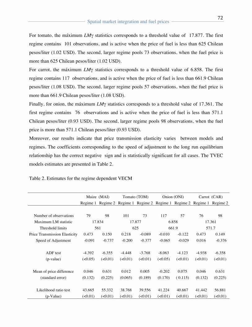
! Spatial market integration and fuel prices
!! !
72!
!
For tomato, the máximum LMγ statistics corresponds to a threshold value of 17.877. The first
regime contains 101 observations, and is active when the price of fuel is less than 625 Chilean
pesos/liter (1.02 USD). The second, larger regime pools 73 observations, when the fuel price is
more than 625 Chilean pesos/liter (1.02 USD).
For carrot, the máximum LMγ statistics corresponds to a threshold value of 6.858. The first
regime contains 117 observations, and is active when the price of fuel is less than 661.9 Chilean
pesos/liter (1.08 USD). The second, larger regime pools 57 observations, when the fuel price is
more than 661.9 Chilean pesos/liter (1.08 USD).
Finally, for onion, the máximum LMγ statistics corresponds to a threshold value of 17.361. The
first regime contains 76 observations and is active when the price of fuel is less than 571.1
Chilean pesos/liter (0.93 USD). The second, larger regime pools 98 observations, when the fuel
price is more than 571.1 Chilean pesos/liter (0.93 USD).
Moreover, our results indicate that price transmission elasticity varies between models and
regimes. The coefficients corresponding to the speed of adjustment to the long run equilibrium
relationship has the correct negative sign and is statistically significant for all cases. The TVEC
models estimates are presented in Table 2.
Table 2. Estimates for the regime dependent VECM
Maize (MAI) Tomato (TOM) Onion (ONI) Carrot (CAR) Regime 1 Regime 2 Regime 1 Regime 2 Regime 1 Regime 2 Regime 1 Regime 2
Number of observations 79 98 101 73 117 57 76 98 Maximum LM statistic 17.834 17.877 6.858 17.361
Threshold limits 561 625 661.9 571.7 Price Transmission Elasticity 0.473 0.150 0.218 -0.089 -0.010 -0.122 0.473 0.149
Speed of Adjustment -0.091 -0.737 -0.200 -0.377 -0.065 -0.029 0.016 -0.376
ADF test -4.392 -6.355 -4.448 -3.768 -8.063 -4.123 -4.938 -6.358 (p-value) (<0.05) (<0.01) (<0.01) (<0.01) (<0.05) (<0.01) (<0.01) (<0.01)
Mean of price difference 0.046 0.631 0.012 0.005 -0.202 0.075 0.046 0.631
(standard error) (0.132) (0.225) (0.065) (0.189) (0.170) ( 0.115) (0.132) (0.225)
Likelihood ratio test 43.665 55.332 38.768 39.556 41.224 40.667 41.442 56.881 (p-Value) (<0.01) (<0.01) (<0.01) (<0.01) (<0.01) (<0.01) (<0.01) (<0.01)
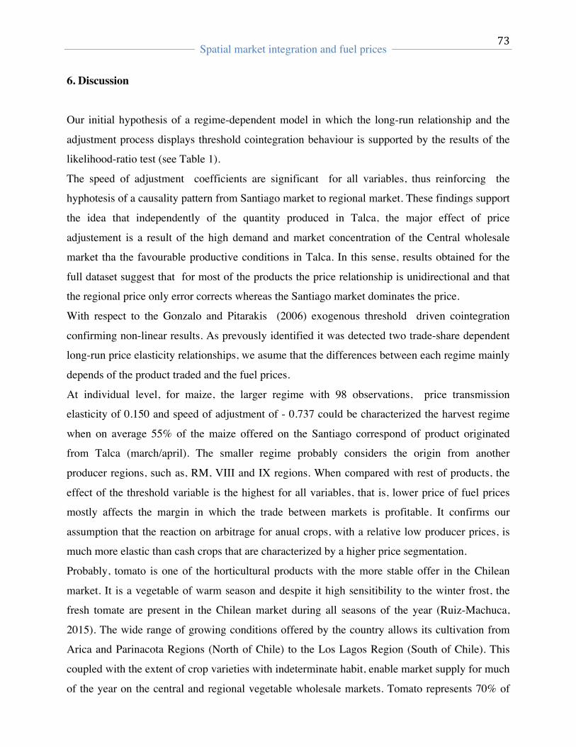
! Spatial market integration and fuel prices
!! !
73!
!
6. Discussion
Our initial hypothesis of a regime-dependent model in which the long-run relationship and the
adjustment process displays threshold cointegration behaviour is supported by the results of the
likelihood-ratio test (see Table 1).
The speed of adjustment coefficients are significant for all variables, thus reinforcing the
hyphotesis of a causality pattern from Santiago market to regional market. These findings support
the idea that independently of the quantity produced in Talca, the major effect of price
adjustement is a result of the high demand and market concentration of the Central wholesale
market tha the favourable productive conditions in Talca. In this sense, results obtained for the
full dataset suggest that for most of the products the price relationship is unidirectional and that
the regional price only error corrects whereas the Santiago market dominates the price.
With respect to the Gonzalo and Pitarakis (2006) exogenous threshold driven cointegration
confirming non-linear results. As prevously identified it was detected two trade-share dependent
long-run price elasticity relationships, we asume that the differences between each regime mainly
depends of the product traded and the fuel prices.
At individual level, for maize, the larger regime with 98 observations, price transmission
elasticity of 0.150 and speed of adjustment of - 0.737 could be characterized the harvest regime
when on average 55% of the maize offered on the Santiago correspond of product originated
from Talca (march/april). The smaller regime probably considers the origin from another
producer regions, such as, RM, VIII and IX regions. When compared with rest of products, the
effect of the threshold variable is the highest for all variables, that is, lower price of fuel prices
mostly affects the margin in which the trade between markets is profitable. It confirms our
assumption that the reaction on arbitrage for anual crops, with a relative low producer prices, is
much more elastic than cash crops that are characterized by a higher price segmentation.
Probably, tomato is one of the horticultural products with the more stable offer in the Chilean
market. It is a vegetable of warm season and despite it high sensitibility to the winter frost, the
fresh tomate are present in the Chilean market during all seasons of the year (Ruiz-Machuca,
2015). The wide range of growing conditions offered by the country allows its cultivation from
Arica and Parinacota Regions (North of Chile) to the Los Lagos Region (South of Chile). This
coupled with the extent of crop varieties with indeterminate habit, enable market supply for much
of the year on the central and regional vegetable wholesale markets. Tomato represents 70% of
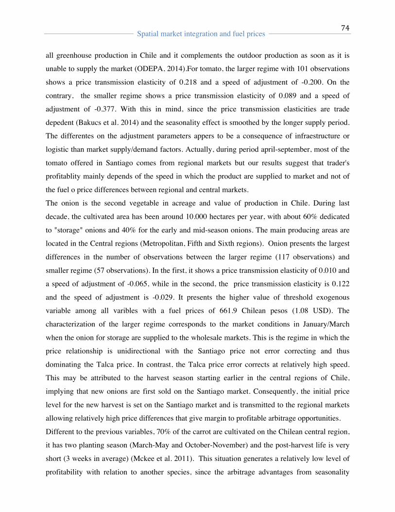
! Spatial market integration and fuel prices
!! !
74!
!
all greenhouse production in Chile and it complements the outdoor production as soon as it is
unable to supply the market (ODEPA, 2014).For tomato, the larger regime with 101 observations
shows a price transmission elasticity of 0.218 and a speed of adjustment of -0.200. On the
contrary, the smaller regime shows a price transmission elasticity of 0.089 and a speed of
adjustment of -0.377. With this in mind, since the price transmission elasticities are trade
depedent (Bakucs et al. 2014) and the seasonality effect is smoothed by the longer supply period.
The differentes on the adjustment parameters appers to be a consequence of infraestructure or
logistic than market supply/demand factors. Actually, during period april-september, most of the
tomato offered in Santiago comes from regional markets but our results suggest that trader's
profitablity mainly depends of the speed in which the product are supplied to market and not of
the fuel o price differences between regional and central markets.
The onion is the second vegetable in acreage and value of production in Chile. During last
decade, the cultivated area has been around 10.000 hectares per year, with about 60% dedicated
to "storage" onions and 40% for the early and mid-season onions. The main producing areas are
located in the Central regions (Metropolitan, Fifth and Sixth regions). Onion presents the largest
differences in the number of observations between the larger regime (117 observations) and
smaller regime (57 observations). In the first, it shows a price transmission elasticity of 0.010 and
a speed of adjustment of -0.065, while in the second, the price transmission elasticity is 0.122
and the speed of adjustment is -0.029. It presents the higher value of threshold exogenous
variable among all varibles with a fuel prices of 661.9 Chilean pesos (1.08 USD). The
characterization of the larger regime corresponds to the market conditions in January/March
when the onion for storage are supplied to the wholesale markets. This is the regime in which the
price relationship is unidirectional with the Santiago price not error correcting and thus
dominating the Talca price. In contrast, the Talca price error corrects at relatively high speed.
This may be attributed to the harvest season starting earlier in the central regions of Chile,
implying that new onions are first sold on the Santiago market. Consequently, the initial price
level for the new harvest is set on the Santiago market and is transmitted to the regional markets
allowing relatively high price differences that give margin to profitable arbitrage opportunities.
Different to the previous variables, 70% of the carrot are cultivated on the Chilean central region,
it has two planting season (March-May and October-November) and the post-harvest life is very
short (3 weeks in average) (Mckee et al. 2011). This situation generates a relatively low level of
profitability with relation to another species, since the arbitrage advantages from seasonality
! Spatial market integration and fuel prices
!! !
75!
!
effect are more difficult to obtain. The larger regime has 98 observations and shows a price
transmission elasticity of 0.149 with a speed of adjustment of -0.376. The smaller regime shows a
price transmission elasticity of 0.473 and a speed of adjustment of -0.016. In this sense, it is not
surprising the similar number of observations between regimes and the sensivitiness of fuel
prices as exogenous threshold. Another interesting statistic differentiating the two regimes is the
mean of price difference and standard deviation. This statistic equals 0.046 in the first regime, but
0.631 in the larger regime suggesting higher volatility of traded quantities during harvesting
season. Following Rodriguez and Hernandez (2005), this effect affect directly the gross margin
obtained by the wholesale markets since the irregular supply behavior and low post-harvest
period of carrot. From our results, we assume a transition effect to carrot producers which also
affect the planting decision and thus, modified their productive structure at farm level. However,
this conclusion is beyod the scope of our article.
7. Conclusions
In this paper, we have analyzed the dynamics of spatial horticultural price transmission be- tween
a central wholesale market (Santiago) and a regional wholesale market (Talca), both located
within a distance of approximately 280 km. The objective is to identify the pathways of
seasonality effects, asymmetries on the price transmission and the role played by the Chilean fuel
prices in horticultural price market integration by the inclusion of a exogenous threshold variable.
We propose a novel procedure to estimate a regime-dependent VEC model accounting for
threshold effects not only in the short-run adjustment towards the long-run equilibrium but in the
long-run equilibrium relationship as well. This method seems to be particularly suitable in
settings of irregular seasonal price transmission, typical for horticultural products.
We found clear evidence of threshold cointegration with Chilean retail fuel prices serving as the
threshold variable. For all variables (maize, tomato, onion and carrot) we identify two price
transmission regimes which are characterized by different equilibrium relationships as well as
short-run adjustment processes towards this equilibrium. Our econometric results fit well with the
actions on the central and regional horticultural markets.
This research could be extended to drilling down the effect of specific public regulations on the
degree of market integration among vegetable markets. For example, since fuel price appears to
be a important variable to take account for the farmer's planting decision, the implementation of
! Spatial market integration and fuel prices
!! !
76!
!
policies oriented to increase the efficiency of the price transmission between markets could affect
positively the gross margin from producers and wholesale market on the commercialization
chain.
Acknowledgements
The authors acknowledge financial support for this research from the Chilean Commission for
Scientific and Technological Research (CONICYT)-Folio No. 21120286.
8. Bibliographic references
Andrews, D. (1993): Tests for parameter instability and structural change with unknown change
point. Econometrica, Vol. 61, pp. 821-856.!
Alam M., McKenzie A., Buysse J., Begum I., Wailes E., Van Huylenbroeck G., 2012. Measuring
Market Integration in the Presence of Threshold Effect: The Case of Bangladesh Rice Markets.
Selected Paper prepared for presentation at the Agricultural & Applied Economics Association
2012 AAEA Conference, Seattle, Washington.
Bakucs, Z and Ferto ̋, I. 2008. Milk market integration in Hungary Horizontal Integration on the
Hungarian Milk Market. In: Csáki Csaba and Forgács Csaba (eds.): Agricultural Economics and
Transition:„What was expected, what we observed, the lessons learned”. Studies on the
Agricultural and Food Sector in Central and Eastern Europe Vol. 44. Leibniz Insitute für
Agrarentwicklung in Mittel and Osteurope, Halle, 2008. pp. 342-352.!
Bakucs, Z., Bojnec, Š., & Fertő, I. (2014). Spatial Product Market Integration between Two
Small, Open Neighbouring Economies. Agribusiness, doi: 10.1002/agr.21399/
Dickey, D. and Fuller, W. A. 1979. Distribution of the estimate for autoregressive time series
with a unit root, Journal of the American Statistical Association, 74, 427–431.
Dillon B. and Barrett C. 2013. Global Crude to Local Food: An Empirical Study of Global Oil
Price Pass-through to Maize Prices in East Africa. External report, International Conference on
Food Price Volatility : Causes and Challenges - Rabat, Morocco
Eryigit, K. Y., & Karaman, S. (2011). Testing for spatial market integration and law of one price
in Turkish wheat markets, Quality & Quantity, 45: 1519–1530. Hansen, B.E. and Seo, B. (2002):
! Spatial market integration and fuel prices
!! !
77!
!
Testing for Two Regime Threshold Cointegration in Vector Error Correction Models. Journal of
Econometrics, Vol.110, pp. 293-318.!
Johansen, S. (1988). Statistical analysis of cointegrating vectors. Journal of Economic Dynamics
and Control, 12(2– 3):231–254.
Kwiatkowski, D., Phillips, P. C., Schmidt, P., & Shin, Y. (1992). Testing the null hypothesis of
stationarity against the alternative of a unit root: How sure are we that economic time series have
a unit root?. Journal of econometrics, 54(1), 159-178.
Mckee, L. H., Myers, B., Leger, J., Lopez, M., & Remmenga, M. (2011). Quality characteristics
of four chile-based fruit spreads developed for home canning. Journal of food processing and
preservation, 35(6), 784-789.
Goetz, L. and von Cramon-Taubadel, S. (2008): Considering threshold effects in the long-run
equilibrium in a vector error correction model: An application to the German apple market.
Contributed paper, 12th Congress of the European Association of Agricultural Economists,
Ghent, Belgium.!
Gonzalo, J. and Pitarakis, J. (2006): Threshold effects in cointegrating relationships. Oxford
Bulletin of Economics and Statistics, Vol. 68 (supplement), pp. 813-833.!
Park A., Jin H., Rozelle S., Huang J., 2002. Market emergence and transition: Arbitrage,
transaction costs, and autarky in China’s grain markets. American Journal of Agricultural
Economics 84 (1), 67–82.
Pede, V. O. and Mckenzie, A. M. (2005). Integration in Benin maize market: an application of
threshold cointegration analysis, Selected paper presented American Agricultural Economics
Association Meeting, Rhode Island, July 24-27.
Pingali, P., Khwaja, Y., Meijer, M., 2005. Commercializing small farms: reducing transaction
costs. ESA Working Paper No. 05-08. Agricultural and Development Economics Division, Food
and Agriculture Organization, Rome.
Ruíz-Machuca, L. M., Ibarra-Jiménez, L., Valdez-Aguilar, L. A., Robledo-Torres, V., Benavides-
Mendoza, A., & Cabrera-De La Fuente, M. (2015). Cultivation of potato–use of plastic mulch
and row covers on soil temperature, growth, nutrient status, and yield. Acta Agriculturae
Scandinavica, Section B—Soil & Plant Science, 65(1), 30-35.


