MARGINAL OPPORTUNITY COST VS. AVERAGE COSTPRICING OF WATER SERVICE:
TIMING ISSUES FOR PRICING REFORM
by
David W. CarterGraduate Research Fellow, University of Florida
andJ. Walter Milon
Professor, University of Florida
Abstract
Average cost (AC) and marginal opportunity cost (MOC) pricing rules are compared forpublic water service in Southwest Florida. A thirty year simulation shows that AC prices are lessthan MOC prices and the difference between AC and MOC prices is greatest around capacityexpansions. These results indicate that the magnitude of the welfare gains available from pricingreform are dependent on the time at which the MOC pricing rule is initiated. In general, theearlier the pricing rule switch is initiated the greater the present value of resource conservationsavings less consumer surplus losses associated with higher MOC prices.
Key Words: water service, pricing reform, marginal opportunity cost, average cost,welfare, water supply, externalities
Staff Papers are circulated without formal review by the Food and Resource EconomicsDepartment. Content is the sole responsibility of the authors.
Food and Resource Economics DepartmentInstitute of Food and Agricultural Sciences
University of FloridaGainesville, FL 32611-0240


Marginal Opportunity Cost vs. Average Cost Pricing Of Water Service:Timing Issues For Pricing Reform
Introduction
Economic theory is clear on the pricing prescriptions for efficient resource use. For
public utilities, this is due primarily to the theoretical and empirical developments in the energy
and telecommunications industries, where much of the theory has also appeared in practice (Berg
and Tshirhart). The theory of efficient utility pricing has yet to be applied with any consistency
in the water service industry. This can be attributed, in part, to the unique features of water
service that are not amenable to the theory-based policies developed in other utility industries
(Hanemann). Mann, however, suggests three, more compelling reasons why theory has not
played a more important role in water service costing and pricing matters:
1. Historically, water service has been provided at lessor cost than other public utility
services and has constituted a relatively small proportion of consumer expenditures;
2. The engineering emphasis common in traditional water supply decision making; and
3. The abundance in the past of inexpensive and easily accessible water supplies (p. 163).
The first two factors are ultimately driven by the third, so that the continued presence of easily
developed water supplies will probably not change the potency of economic theory in water
service pricing practices. On the other hand, in areas where the inexpensive supplies are
relatively scarce and the long run costs of capacity expansion are rising, economic theory will
have more practical appeal. In these more critical situations, the relative benefits of moving to
more efficient pricing practices need to be evaluated in the context of other resource management
1
strategies.
Water Service Pricing Theory and Practice: an Overview
Water service in the United States has traditionally been priced at average or 'embedded'
cost (Beecher, Mann and Landers; LaFrancois; Mann). Average cost pricing has no basis in
economic efficiency (Baumol, Koehn, and Willig; Hall and Hanemann) and will lead to a
wasteful use of resources where the marginal opportunity cost (MaC) of water service is rising
(Hirshleifer, DeHaven, and Milliman). It is not clear, though, that water service pricing rules in
practice, even those with conservation goals, bear any relation to the marginal opportunity costs
of service (Hanke 1978). Subsequently, existing pricing rules, based on average costs, may
produce prices that diverge significantly from marginal opportunity costs.
According to Mann, "(t)he neglect of pricing and costing matters has produced the
general underpricing of urban water service in the United States" (p. 164). Others have
expressed similar concerns, implying that, in practice, water service prices are less than marginal
opportunity costs (Mann and LaFrancois; Mercer and Morgan; Moncur and Pollock 1988,
1995). Despite these claims of underpricing, there have been few attempts, if any, to assess the
welfare implications of applied pricing reform that would encourage efficient long-run resource
use. Previous pricing reform welfare analyses have focused on the move to efficient short-run
pricing (Kim; Renzetti ), peak load pricing (Feldman, Breese, and Obeiter; Hanke 1982), and
optimal price solutions to the pricing-investment problem (Dandy, McBean, and Hutchinson
1984, 1985; Riordan 1971a,b; Russell and Shin 1996a,b; Swallow and Marin). This paper
examines the implications of a switch from average cost to marginal opportunity cost pricing for
water service in the context of Florida's water management system. In particular, it is shown that
2
the timing of pricing reform can affect the magnitude of potential welfare improvements
available.
Pricing Rules
average cost pricing
The traditional strategy in water service pricing is to set rates to ensure that the revenue
generated from water sales is sufficient to cover total system costs (AWWA). Because this
strategy ensures that total revenues equal total costs, average revenue or price will equal average
cost. To see this, define the total annual revenue requirements (net of directly attributable system
costs) for a water utility serving a single customer class with uniform demand (non-peaking)l as
R(q) =[q (g)·c] +Dt (-1 t t (1)
where qt-l is the previous year's aggregate water use, g is a growth rate, and Ct is the anticipated
marginal (average) operating cost per unit. Dt is the annual debt service given by
t
D =" fer)t L.-t tt=1
(2)
where It is the investment in capacity in year t and r is the capital recovery factor. The average
cost price is simply the annual revenue requirements divided by the annual total quantity of water
use or
3
AC R(q)tp =--
t qt
subject to a break-even constraint
p ACeq =(c eq ) +Dt t t t t
The break-even constraint is added here to reflect the goal of self-sufficiency and fiscal
(3)
(4)
responsibility expected of publicly owned utility services and the ideal of setting rates to recover
strictly the costs of service (AWWA; Freedman). In practice, however, some municipalities may
view their utility operations as a "money-maker" (Goldstein), whereas others are inclined to
provide subsidies to keep rates low (Hite and Ulbrich).
The general average cost pricing rule in (3) presents the allocation of shared costs on the
basis of (relative) output. This is an oversimplification in that it assumes all costs are collected
in the variable price. In practice, many cost/revenue service functions (e.g. customer costs, hook-
up costs) are collected as various fees and not recovered in the unit charge (Mckay et al.).
However, because (3) captures the spirit of the allocation process, it will be used as a point of
comparison with the marginal opportunity cost pricing rule discussed below.
Marginal opportunity cost pricing
The optimal pricing-investment strategy for water system expansion requires
simultaneous selection of prices and the timing of capacity increments. In this case, according to
Riordan (1971a), "the particular value of marginal cost relevant for expansion cannot be
4
determined prior to finding the optimal solution to the problem; it is equal to an internal shadow
price that is a product of the analysis" (p. 248). The solution calls for a series of price
fluctuations to signal coming capacity increments and ration existing capacity (Riordan 1971b).
However, the large variations (up and down) in the price level that can occur over time,
especially where relatively large capacity elements are considered, may be politically
unacceptable. Research has shown that it may be possible to either constrain (Dandy, McBean,
and Hutchinson 1984, 1985) or"smooth" (Swallow and Marin) the price paths without
significant welfare losses from the optimal case.
Even if the large price fluctuations could be constrained or smoothed to politically
acceptable fluctuations, it would be difficult to effect the efficient investment-pricing rule in
practice for at least two reasons: (1) water service is priced by water agencies and regulators and
not by the market and (2) water use behavior takes time to fully respond to price changes. There
are no fully competitive markets for retail water service that can automatically adjust prices to
ration scarce system capacity and signal capacity expansion.2 Furthermore, significant
reductions in water use take time and are often permanent or 'hard' and unlikely to respond (back
and forth) neatly to the price fluctuations in the optimal investment-pricing model (Hall). Rate
makers could, of course, attempt to set market-clearing prices given perfect information about the
water demand function(s) of their customer base. Without this information, though, efficiency
minded rate-makers can only approximate market prices for water service. The formulation of
marginal cost is critical in this respect: Prices that encourage truly efficient water resource use
are set to approximate as nearly as possible the marginal opportunity costs of water service. In
addition, it is important for system planners to account for the peculiar ways in which demand
5

may respond (e.g. hardening) to cost/price changes.
An effective approximation of the efficient investment-pricing rule will emulate the
rationing-signaling effect of the market and account for the full range of marginal opportunity
costs associated with a unit of water use. The marginal opportunity cost framework for resource
valuation has been adapted for both water service (Warford) and electricity supply pricing
(Munsinghe and Schramm) and appears generally as
MOC =c +C +E +ut t t t t
where Ct is marginal operating cost, Ct is marginal capital cost, Et is marginal external or
environmental cost, and ~ is marginal user cost.
Marginal capital cost (MCC) is not well defined for utility services due to capital
(5)
indivisibilities (Crew and Roberts; Williamson) and must be approximated. Saunders, Warford,
and Mann presented an early review of approximations to MCC in the presence of
indivisibilities. Russell and Shin (1996a,b) capture the important features of their findings and
add considerably to the understanding of the MCC formulae: textbook marginal cost (TMC),
Turvey marginal cost (TVMC), and average marginal cost (AMC). These three formulae all
focus on future water supply and cost circumstances, however, they differ in the way in which
they make future capital costs marginal to current consumption decisions. Russell and Shin
(1996b) find that TMC, TVMC, and AMC perform reasonably well (i.e. they produce favorable
net benefits over the existing pricing rule) when the capacity increments are arranged optimally
over the planning horizon via a dynamic programing application. Performance is mixed, though,
when capacity increments are not optimally configured. The welfare performance of AMC is not
6

significantly affected by the optimallity of capacity timing, whereas the welfare improvements
available from TVMC are dramatically reduced. This makes intuitive sense because the TVMC
method is formulated in the time dimension where efficiency distortions can easily occur from
capacity increments out of synch with demand or projects being developed out of least-cost
order.3 In addition, AMC yielded greater present value net benefits than TVMC and TMC (and
the existing pricing rule) in both situations and produced less price variation over time. In light
of these results, AMC is the choice formulation ofMCC for the present research.
The AMC formulation of MCC fashions a compromise between the efficient price signal
and political constraints on price fluctuations by averaging the present value sum of unit
investment costs over the planning horizon. The averaging acts to "smooth out lumps in
expenditure streams while at the same time reflecting the general level and trend of future costs
which will have to be incurred as water consumption increases" (Saunders, Warford, and Mann
p. 27). Russell and Shin (1996a) present AMC as
T I ~L (r) t+t ~
1 t=k (1 +i)t-kMCC =AMC ----------
t t (1 +i) k - t T D.Q ~L t~t
t=k (1 +i)t-k
where I is the capital cost of capacity increment D.Q, i is the discount rate, and r is the capital
(6)
recovery factor. Subscript k denotes the very next capacity added year after t and subscripts 1
through T denote every other year over the planning horizon.4
Marginal external cost (MEC) is meant to represent any current cost(s) caused by the use
of a unit of water that is not reflected in the marginal (private) operating cost of water service.
7
These external costs are generally in the form of (current) forgone valued use opportunities for a
resource unit when it is devoted to water service. For example, water withdrawn from a
interrelated ground-surface water system is no longer available to maintain wetland ecology. To
the extent that wetlands are valuable, the value of any wetland loss due to groundwater
withdrawal is an opportunity cost of groundwater use. In this case, it is efficient to withdrawal
groundwater to the point where the marginal value of wetlands forgone is equal to the marginal
benefits gained when the groundwater is employed in another valued use, like for public water
supply. Figure 1 (adapted from Thomas and Martin) demonstrates how the equalization of
marginal values could stabilize groundwater withdrawal levels and wetland loss in the presence
of growing demand for public water supply.
Groundwater system development is shown as a function of the water table depth d associated
with a specific level of ground water withdrawal Q. Groundwater withdrawal equals recharge at
the maximum sustainable yield (MSY) at quantity Q*. At MSY wetlands near concentrated
wellfield pumping are eliminated since they represent a major source of evaporation losses in the
interrelated ground-surface water system (Serrano and Serrano; SWFWMD). The relationships
among the graph quadrants are as follows:
I. The quantity of groundwater withdrawn is determined at the intersection of the demand
curve D and the private marginal operating cost (ct) curve C in quadrant I. Note that C is
the short-run marginal cost of water production and is vertical at the MSY of the aquifer
due to regulations on groundwater withdrawal and/or water system capacity limits;
II. The quantity of water withdrawn determines the depth to the groundwater table with the
stock function SeQ) in quadrant II;
8

III. The depth to the water table specifies the amount of groundwater not available for
wetland sustenance in quadrant III. The existing stock of wetlands (measured on the
negative half of the horizontal axis where 0 is the maximum stock) is a function WeD) of
the depth to the water table; and
9

Figure 1. Groundwater System Equilibrium in the Presence of EnvironmentalExternalities (adapted from Thomas and Martin)
B(w)
Less~etlands
stock ofwetlands, W
W(d)
IV
- ....--
III
marginal value andmarginal cost of
groundwater for publicsupply and wetland
sustanence
A
p*2
DEEP
I
--~
II
MSY
C
- - -- ~-----.Q2 Q* Quantity of
groundwaterwithdrawn,Q
S(Q)
depth to the water table, d
10

IV. The benefits of (demand for) wetlands is a function B(W) of the available wetland stock
in quadrant IV.
At withdrawal levels between 0 to Qe, marginal external costs are negligible and marginal private
costs equal marginal social costs. For instance, at DI, the equilibrium price and quantity are PI
and QI, respectively. Following QI down to the stock function in quadrant II, across to the
wetland loss function in quadrant III, up to the wetland benefit function in quadrant IV, and
finally across to the price axis we see that the value of wetlands stock (loss) or marginal external
cost is roughly equal to the marginal private cost price Pl. However, withdrawal of the MSY
quantity Q* to meet demand D2at the marginal private cost price, P2, leads to a drop in the water
table, a loss of (water available for) wetlands, and an increase in marginal external costs to P2*
(including the MPC). At this point, if the price remains equal to the marginal private cost, P2, the
system is out of equilibrium and a social efficiency loss occurs equal to the shaded triangle:
water users are over consuming because the value of Q2 - Q* to them is less than the social cost
(marginal private cost + lost wetland benefits). The system can be brought back into equilibrium
two ways. The first would be to internalize the marginal external costs in the price for water
service by charging P2*for a unit of water so that a quantity, say Q2' between Qe and Q* is
demanded. Revenues collected over total private costs could be used to somehow compensate
for the lost wetland benefits or to mitigate the wetland damage. The former would be the Pareto
superior option, but the lack of knowledge about the wetland damage (benefits) function and the
likely confusion surrounding payment of compensation make the option of mitigation more
appealing in practice. However, it may be that the uncertainty associated with mitigation success
is such that regulatory agencies charged with protecting wetland systems may set groundwater
11
withdrawal limits or quotas to prevent rather than allow mitigation of wetland damage (Baumol
and Oates 1989, Chapter 5). For example, pumping restrictions, like those considered recently to
protect Florida's groundwater systems, would appear in Figure 1 as a leftward movement of Q*
which would now represent the maximum allowable system capacity. Ideally, the withdrawal
limitation would be set where the marginal value of groundwater withdrawal for public supply
use given by D2 equals the marginal value of groundwater to maintain wetland stocks (possibly at
Q2). With stable demand this leftward movement of Q* prohibits withdrawal quantities that
cause wetland losses, thereby reducing or eliminating MECs. Some combination of withdrawal
limitations and wetland mitigation requirements could also achieve (quasi) equilibrium ifthe
mitigation costs are included in the marginal charge for water service. The Florida case study
considered below is a hybrid approach on this order.
Marginal user cost. Marginal user cost (MUC) is an opportunity cost of water service in
terms of valued future use opportunities forgone for a unit of water of present quality at present
cost. This opportunity cost becomes significant in water service where it is anticipated that
potable water production is to be more costly (ct + Et) in real terms at some point in the future.
Here we are concerned with the ability of the existing water system to meet the demands of
future customers. On equity grounds it can be argued that future customers are entitled to
potable water service at a real (social) cost no greater that incurred by present customers, ceteris
paribus (Hanke and Wenders). Subsequently, where it is expected that in the foreseeable future
an additional unit of potable water will cost more to produce and deliver than it does presently,
the current costs/prices for water service should reflect the relative scarcity of the resource
(Martin et al.; Moncur and Pollock 1988).
12

Exhaustible resource theory presents scarcity rent or user cost as the difference between
the market price and the marginal extraction cost of a resource (Heal). This approach is not
strictly applicable for water service because, as discussed earlier, retail water service prices are
"set" and not market determined. With this problem in mind Moncur and Pollock (1988)
develop a simple expression of user costs for water service:
*c -cMUC - T t
t e i(T-t)
where i is the (social) discount rate, and c*t and c*T are, respectively, the social marginal
(7)
operating costs (including external costs, i.e. Ct + Et) of water service today (period t) and at the
end of the planning horizon (period T) when the replacement or backstop technology is brought
on line. Note that this user cost adaption for water service follows in the spirit of the formulation
commonly used in applied analyses of energy resource pricing and investment (e.g. Schramm or
Hohmeyer). Marginal user cost in (7) is the present value magnitude of the difference between
the marginal (social) cost of water service in period t and at the end of the planning horizon T
with the backstop technology. This is essentially a compromise between the lower bound on
water resource opportunity cost given by the current marginal social cost c*t and the upper bound
on opportunity cost at the replacement marginal social cost c*T' The present value connotation
supposes that the MUC and, thus the efficient price of water service (because P == c*t + ~), will
move over time in accordance with the interest rate, depending on the path of c*t. Symbolically,
with an efficiency price Pt given as
13

*c -cT t
P =c +--t t e i(T-t)
and assuming c*t constant, the rate of change in the efficiency price for water service is
P t + 1 - P tP
(8)
(9)
This the familiar Hotelling rule that the market price of an (exhaustible) resource must grow at a
rate equal to the rate of interest. In effect, then, the MUC formulation in (7) assumes market
characteristics on the behavior of water system costs and prices over time. Also, note that user
costs are sensitive to (expectations about) the rate of technological change and the social cost of
the backstop: an increase (decrease) in the marginal social cost C*T of water from the backstop
technology will increase (decrease) the user cost of consumption from existing water supplies.
The user cost formulation (7) estimates a marginal opportunity cost of present water
resource use and is not a measure of the (scarcity) value of water resources: value or scarcity
value can only be expressed by what the water demander is willing to sacrifice to either use or
conserve scarce water resources. Scarcity values, where present, represent an upper bounds on
the amount of user cost or scarcity rent that can be generated through water service fees (Moncur
and Pollock 1989). Subsequently, the collection scarcity rents or user costs in water service may
be less important where scarcity values for water resources are effected through other
mechanisms, say via institutional action (Lynne).
The expanded definition of the marginal opportunity cost of water service given in (5) is
14

MOC =c *+1---t t (l+i)k-t
T I "L (r) t+t"
t=k (1 +i)t-k------+
T ~Q"L t~t
t=k (1 +i)t-k
*c -cT t
e i(T~t)
(10)
where the notation is as presented above (note that c* includes marginal external costs).
Average Cost vs. Marginal Opportunity Cost
Consider the differences between the AC pricing rule in (3) and the MOC pricing rule in
(10):
Difference 1: The MOC rule explicitly considers external costs as a part of short run marginal
costs c, whereas the AC rule may not.
Difference 2: In the MOC rule, (unattributable) capacity expansion costs are collected in the
marginal price prior to the capacity start-up (second term). The AC rule collects
(unattributable) capacity expansion costs as an average (in SC) after the capacity
is in place (second term).
Difference 3: The MOC rule recognizes future opportunity costs with a user cost component
(third term), the AC rule does not.
The first difference will only be significant to the extent that average cost accounting methods in
practice do not consider the external costs of water service. In many areas, regulations require
water suppliers to mitigate external costs, such as those associated with environmental
degradation. Where this occurs external costs become (approximately) internalized in
accounting practices and, therefore, appear in AC prices.5 Whether these mitigation costs are
15

collected at the margin in c or as an average as part of shared costs is not likely to change the
end-use average price. Where the mitigation costs are collected in fixed charges, though,
potential signaling benefits would be dampened or eliminated because marginal consumption
decisions are not fully informed about the marginal external costs of water use. Regulatory
action could also function to prevent external costs by imposing restrictions on water use
(withdrawal) from a particular source to avoid the damaging levels of use. In such cases,
external costs are reduced or eliminated and will not contribute to the divergence between AC
and MaC prices.
The second difference between the AC and MaC rules is a matter of timing, that is, both
rules account for all capacity expansion costs, it is just a matter of when. The MaC rule charges
a MCC for capacity costs ahead of time in order to preserve signaling benefits and consumer
choice. The MCC component of MaC is, in theory, highest just before a capacity expansion,
lowest after a capacity element is installed (sunk) and will be zero when no future capacity
investment is planned. On the other hand, the AC rule does not charge for capacity expansion
until the investment can be considered "used and useful" and/or debt service payments begin to
factor into the revenue requirements.6 Therefore, the AC rule exhibits the lowest prices
(assuming economies of scale) just before capacity expansion and the highest prices right after
capacity is installed. This timing schedule works completely counter to economic efficiency as
water use is encouraged with relatively low prices when capacity is scarce and discouraged with
relatively high prices when surplus capacity exists.
The third difference between the AC and MOC pricing rule reflects the notion that
marginal user costs are typically not included in traditional AC water service prices (Moncur and
16

Pollock 1988). Higher user costs will, of course, mean higher MOC prices and a greater
divergence between AC and MOC prices. From (6), the magnitude ofmarginaillser cost in any
period t will depend on the spread between current system marginal (social) costs and future
system marginal (social) costs with the replacement (backstop) technology (C*T-C*t)' ceteris
paribus.
With the above said, we can specify four conditions regarding the difference between AC
and MOC prices:
1. We cannot say a priori what effect the magnitude of external costs will have on the
difference between AC and MOC prices. To the extent that water suppliers are required
to mitigate external costs, these costs will be included in system accounts and in the AC
price for water service. In these cases, the difference between MOC and AC prices will
depend on whether mitigation costs are collected with fixed charges or at the margin.
2. The divergence between AC and MOC prices will be most significant just after and, more
importantly, just before a capacity expansion. Before (after) capacity expansion
MOC>AC (MOC<AC).
3. For any period, the divergence between AC and MOC prices depends on the degree to
which (real) historic and future capacity expansion costs differ. Relatively higher (lower)
future costs suggest MOC>AC (MOC<AC).
4. For any period, the divergence between AC and MOC prices depends on the magnitude
of the difference between current system marginal (social) cost and future system
marginal (social) cost with the replacement (backstop) technology. We cannot say a
priori whether high (low) user costs will have MOC>AC (MOC<AC).
17

The potential welfare improvements available from MOC pricing in an area will depend
(unambiguously) on conditions two and three. Assuming that condition three is significant (i.e.
new supply costs are greater than historic capacity costs) the consequences of maintaining the
AC rule will be most noticeable before and after capacity expansions.
Simulation
The analysis considers the definition of average cost (AC) pricing presented in equations
(1) through (4) and three definitions of marginal opportunity cost (MOC) based on equation (10).
The MOC price formulas range from a basic formulation (MOC 1) that includes only marginal
operating and capital costs to a "fully-loaded" formulation that includes external cost and user
cost components. Symbolically,
MOC] =c +Ct t
MOC2=c +C +Et t t
MOC3 =c +C +E +ut t t t
For the AC and MOCI formulations, any external costs of water service that have been
(11)
(12)
(13)
internalized (e.g. as environmental mitigation costs) are assumed to be collected through fixed
annual or monthly fees that in total equal
(14)
where the notation is as described above. Depreciation and inflation are assumed to be zero (on
net) for all pricing simulations over the planning horizon.
18

Study area and background
The AC and MOC formulae set forth in the previous section are simulated using data
from the West Coast Regional Water Supply Authority (now known as Tampa Bay Water,
hereafter WCRWSA) in Southwest Florida. The WCRWSA wholesales raw and potable water
at cost to six member governments who, in turn, provide retail water service to 1.8 million
residents in the area surrounding Tampa Bay, Florida. In 1995, the WCRWSA averaged 127.6
million gallons per day (mgd) of water production from eleven wellfields throughout the region.
This supply in combination with water production from member operated facilities (93.7 mgd)
provided over 220 mgd in 1995 to meet water demands in the region. The total existing capacity
in the region is 311.7 mgd and regional water use is anticipated to grow to 304 mgd by 2015 and
344 mgd by 2030 (Law Environmental in association with Havens and Emerson). Subsequently,
new capacity will be "needed" before 2015. The supply deficit may be more or less significant
in certain areas depending on the degree of interconnection and the location of new capacity
additions.
The WCRWSA is responsible for the development of new water regional supply sources
on behalf of its member governments (Regional Water System Contract). Any new supply
sources will add capacity to the so-called Regional System production that is shared in
"common" by the member governments. Since member governments cannot develop their own
new water supply sources the cost of new water supplies to the regional system defines the long
run marginal cost of potable water in the region. During 1994, the WCRWSA developed a
Water Resource Development Plan (RDP) to evaluate the future water supply options in the
regIon. The RDP concludes with a suggested Master Water Plan that specifies a strategy for new
19

capacity additions through the year 2030, including rather detailed estimates of costs associated
with various capacity increments that were used in the present analysis
We simulate wholesale MOC and AC prices for water from the Regional System using a
static (i.e. "non-optimized") capacity expansion plan (see Table 1).7 However, as noted
previously, recent research suggests that the net benefits of pricing with the average marginal
cost formulation of MCC used in the present study are relatively insensitive to the optimality of
the capacity expansion plan (Russell and Shin 1996b). The estimated wholesale water prices are
then converted to (uniform) retail prices to evaluate the net benefits of efficient pricing in the
Tampa Bay region. 8
Backstop technology
A backstop technology must be identified in order to calculate the user cost component of
marginal opportunity cost. The backstop technology considered in this analysis is a 32 mgd
seawater desalination plant (see Table 1). Desalination is not the only potential backstop water
supply in the study area. Long distance interbasin water transfers have also been considered as a
backstop source. However, desalination is being pursued before such transfers under the guise of
a "local sources first" policy instituted by the SWFWMD and Florida water law. This policy
stipulates that Gulf water desalination is a local source and must be examined before long
distance inter-basin or inter-district transfers are considered. Given that the marginal operating
cost of desalination ($3.62) is more than twice that estimated for a comparable supply via inter
regional transfer ($1.56 for a transfer from Lake Rouseau to the north), the decision to pursue
desalination before transfers is not basedpurely on least engineering costs.9 Therefore, policy
20

makers are implicitly recognizing other socioeconomic and political opportunity costs associated
with the long-distance transfer that are not considered in the engineering cost estimates.
There remains the question of technological improvements that may affect (lower) the
cost of water from the backstop. A report on desalination prepared for the California Urban
Water Agencies (Boyle Engineering 1991) includes an entire section on the "potential for
technology improvements" in which it is concluded (p. 43): "Although there will undoubtedly be
some improvements (in desalination technology), the only 'breakthrough' that is likely to result in
major cost reductions would be the development of a cheaper power source." This applies to
both membrane and distillation desalination processes. Consequently, predictions about future
cost savings in the desalination process appear to require speculations about the cost of electricity
and energy in general. Nonesuch speculations are made for this analysis, although, we could
assume that any cost savings from technological improvements are offset by increases in energy
costs. In any case, it is assumed that the marginal operating and environmental costs (c + E) of
water from the WCRWSA Regional System reach a maximum by 2030 and thereafter remain
constant (or decline) into the indefinite future. In other words, specification of seawater
desalination as the backstop technology is legitimate. If it turns out that costs actually continue
to rise, then the marginal user cost and associated marginal opportunity costs calculated here will
be understated. Subsequently, our estimates can be considered a lower bounds on potential user
cost for water service in the study area.
21
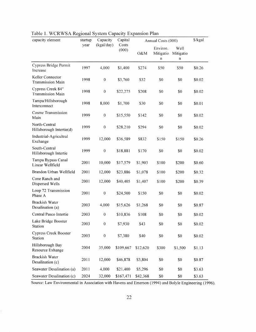
Table 1. WCRWSA Regional System Capacity Expansion Plancapacity element startup Capacity Capital Annual Costs (000) $/kgal
year (kgal/day) Costs(000) Environ. Well
O&M Mitigatio Mitigation n
Cypress Bridge Permit1997 4,000 $1,400 $274 $50 $50 $0.26
Increase
Keller Connector1998 0 $3,760 $32 $0 $0 $0.02
Transmission Main
Cypress Creek 84"1998 0 $22,275 $208 $0 $0 $0.02
Transmission Main
Tampa/Hillsborough1998 8,000 $1,700 $30 $0 $0 $0.01
Interconnect
Cosme Transmission1999 0 $15,550 $142 $0 $0 $0.02
Main
North-Central1999 0 $28,210 $294 $0 $0 $0.02
Hillsborough Intertie(d)
Industrial-Agricultral1999 12,000 $36,589 $832 $150 $150 $0.26
Exchange
South-Central1999 0 $18,881 $170 $0 $0 $0.02Hillsborough Intertie
Tampa Bypass Canal2001 10,000 $17,579 $1,903 $100 $200 $0.60Linear Wellfield
Brandon Urban Wellfield 2001 12,000 $23,886 $1,078 $100 $200 $0.32
Cone Ranch and2001 12,000 $40,405 $1,407 $100 $200 $0.39Dispersed Wells
Loop 72 Transmission2001 0 $24,500 $150 $0 $0 $0.02Phase A
Brackish Water2003 4,000 $15,626 $1,268 $0 $0 $0.87Desalination (a)
Central Pasco Intertie 2003 0 $10,836 $108 $0 $0 $0.02
Lake Bridge Booster2003 0 $7,930 $43 $0 $0 $0.02Station
Cypress Creek Booster2003 0 $7,380 $40 $0 $0 $0.02Station
Hillsborough Bay2004 35,000 $109,667 $12,620 $300 $1,500 $1.13Resource Exhange
Brackish Water2011 12,000 $46,878 $3,804 $0 $0 $0.87
Desalination (c)
Seawater Desalination (a) 2011 4,000 $21,400 $5,296 $0 $0 $3.63
Seawater Desalination (c) 2024 32,000 $167,471 $42,368 $0 $0 $3.63
Source: Law Environmental in Association with Havens and Emerson (1994) and Bolyle Engineering (1996).
22

Demandfor Water in Southwest Florida
The single family demand model Io used to compare AC with MOC pricing rules is based
on an analysis of water use in Southwest Florida (Brown and Caldwell in association with John
Whitcomb) and measures the percentage change in a base single family water use qbsf due to
percentage changes in combined water and sewer prices P:
Base water use qbsf is a function of an intercept, persons per household, net irrigation
(15)
requirements, irrigation restrictions, lot size, and the existence of an irrigation well or pool. 11
The percentage changes in price are measured with deviations from the maximum sample price
of$7.05/kgal and price responsiveness is given by the parameter estimates pI and p2. In this
way, the model is flexible, allowing price elasticity to vary with price level. I2 Note, however,
that elasticity is forced to zero at a price of $7.05.
The difference Dq between single family daily water demand with average cost prices
D(PAC) and the demand with marginal opportunity cost prices D(PMOC) is given by
D = D(P ) - D(P )q MOC AC
In terms of the single family demand equation in (18), this difference is
23
(16)

PMOCi
f1q sf,t IPAC
sf * ( [l+ A * (7.0S-P )~2] - [l+P* (7.0S-P l2])qB PI MOCi I AC
(17)
The water use responses to price changes measured in the Southwest Florida demand study
reflect long-run adjustments in water use patterns. This is significant for the present analysis in
two ways: (1) the full quantity changes in water use with respect to price cannot be expected to
appear immediately (less than a year) following a price change, and (2) the price responsive
changes in water use behavior will reflect long-run (opportunity) values for water service. The
first point suggests that year to year water use changes due to price changes should be taken with
caution and may be viewed as over or under estimates of actual responses depending on the
direction of the price change. The second point is important because the relevant measure of the
long-run (marginal or average) costs for water service should include customer investments in
water efficiency (Hall). Changes in water use patterns in the long-run include customer
investments in water efficiency and, therefore, are indicative of the cost (value) of conservation
to the customer relative to the (opportunity) cost of new capacity development. Prices based on
(forward-looking) marginal opportunity costs act to maximize the benefits from this trade-off.
The final estimates of per unit single family household and commercial water use are "grossed
up" to determine the WCRWSA Regional System water use and net revenues with the different
price formulations. 13
Welfare measures: relative net benefits ofpricing rules
Single family households are used to "gauge" the relative net benefits available with a
24
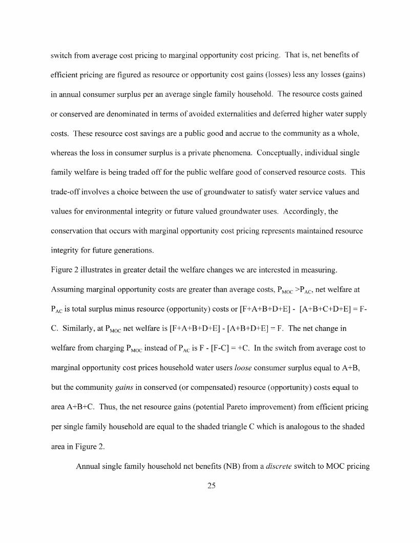
switch from average cost pricing to marginal opportunity cost pricing. That is, net benefits of
efficient pricing are figured as resource or opportunity cost gains (losses) less any losses (gains)
in annual consumer surplus per an average single family household. The resource costs gained
or conserved are denominated in terms of avoided externalities and deferred higher water supply
costs. These resource cost savings are a public good and accrue to the community as a whole,
whereas the loss in consumer surplus is a private phenomena. Conceptually, individual single
family welfare is being traded off for the public welfare good of conserved resource costs. This
trade-off involves a choice between the use of groundwater to satisfy water service values and
values for environmental integrity or future valued groundwater uses. Accordingly, the
conservation that occurs with marginal opportunity cost pricing represents maintained resource
integrity for future generations.
Figure 2 illustrates in greater detail the welfare changes we are interested in measuring.
Assuming marginal opportunity costs are greater than average costs, PMOC >PAC, net welfare at
PAC is total surplus minus resource (opportunity) costs or [F+A+B+D+E] - [A+B+C+D+E] == F
C. Similarly, at PMOC net welfare is [F+A+B+D+E] - [A+B+D+E] == F. The net change in
welfare from charging PMOC instead ofPAC is F - [F-C] == +C. In the switch from average cost to
marginal opportunity cost prices household water users loose consumer surplus equal to A+B,
but the community gains in conserved (or compensated) resource (opportunity) costs equal to
area A+B+C. Thus, the net resource gains (potential Pareto improvement) from efficient pricing
per single family household are equal to the shaded triangle C which is analogous to the shaded
area in Figure 2.
Annual single family household net benefits (NB) from a discrete switch to MOC pricing
25

in year t are given by
PMOCi
NB t =[(PMOCi -PAC)oq(PAC)] - I:1cs f q(P)dP
PAC
(18)
where the first term on the right measures the resource cost of use level q(PAC) (area A+B+C) and
the second term measures the area under the demand curve between PAC and PMOC (area A+B).
Integrating equation (18) from PAC to PMOC gives the annual change in consumer surplus:
PMOCi
NB =6CS = f Q(P)dpt t
PAC
(19)
This Marshallian welfare measure of equivalent variation is used because compensation variation
cannot be measured due to the lack of an income parameter in the demand model. 14 The discrete
26

Figure 2. Measurement of the Net Benefits from a Switch to MOC Pricing
p
F
DE
Q
measure of net benefits shows the relative net annual benefits from efficient pricing available in
any given year over the planning horizon. However, given that pricing policies are rigid in
practice and not apt to switch from year to year, a more practical indicator of the benefits of
efficient pricing is the present value net benefits of a permanent switch to MOC pricing in year t
T
PVNB ~=" NB ~t ~ t+t
t=t
27
(20)

This formulation of PVNB accounts for the fact that benefits may be lost (or gained) by
postponing (accelerating) the time at which the switch to marginal opportunity cost pricing takes
place.
Results and Discussion
Price Path Stability
Table 3 presents the coefficients of variation for the AC and MaC price paths.
Coefficient of variation (On_l/X) is a measure of the variability of the prices about the mean for
the planning horizon. It expresses the standard deviation of the price paths as a function of their
means. The coefficients in Table 3 show that the MaC price paths are remarkably consistent
about the mean, though this does not necessarily indicate that the paths are stable. Russell and
Shin found coefficient of variation for the average marginal cost formulation of 24%. Their
formulation is comparable with our MaC1, which showed a high coefficient of variation of 6.6%
and a low of 6.2%.
Table 4. Coefficients of Variation for the Estimated Price Paths from 1996 to 2030
interest rate
.03
.07
MOC1
6.2
6.6
Coefficients. of Variation (%)
MOC2 MOC3
8.1 6.6
7.9 8.9
28
AC
11.8
12.8

Figure 3 presents the predicted AC and MOC price paths over the planning horizon with a .07
interest rate. In the figure we see that the relatively low coefficients of variation for the MOC
paths occur because price increases are typically matched with equivalent (or greater) price
decreases over the planning horizon. This price variation acts to ration scarce capacity before
system expansions and to signal the efficient timing of expansions. In this way, the MOC
formulations emulate the efficient pricing-investment path estimated by Riordan (1971b). Note,
Figure 3. Marginal Opportunity Cost and Average Cost Price Paths
$ 3. 5 -,----------------------------~------------------------------- -------------------------- -- ----- ------ -
S3 -+------------------------------------------------------ -----------------------------------------------------------
2014 2017 2020 2023 2026 2029
$2.5 -'----------------.------------------------------------------------------------'-"~----------------------------------------~----
.' .. ' .
SO --+----------,----- ----------r-----· -------------,--------------- --,--------- ----,--------
1996 1999 2002 2005 2008 2011
~ / \~...~ /" ./ . .
$1. 5 -~--~~~---.------I--:~:~.~..: .,... -~-\;: :::.:-.~;;i ....,...··
t.:·,.~ ~"":"~ :.: "'" .Sl +--------------1----------------------- --------------------------- ------ ---. -- ------------- --
II
SO.5 1I
I
S2 --+----~-- ------ ------------------------~----I-----------.--.------------ --.---------
/'/ :.\. ... /" ..,.'.. /
year
-- AC ............. MOC1 MOC2 -.- MOC3
29

however, that in most cases the MOC price paths fluctuate within a reasonable bounds (within
roughly $.50) and it is single year price decreases, not increases, that are most intense. The
narrow band of price fluctuation is due to the blending of system costs. That is, price
fluctuations would sharpen if the Regional System wholesale MOC prices were considered
independent of other area supply source costs. The relatively dramatic price decreases occur
after capacity expansion when the preceding capital investment is removed from the price signal
because it is no longer marginal (avoidable) to water use decisions. As long as expansion or
replacement capacity is anticipated in the future, though, there will still be a marginal capital cost
element in the MOC price signal.
The coefficients of variation for AC prices are relatively high due to the large price
increases that occur in years when capacity is added (see spikes in Figure 3). The high capital
and operating costs of the backstop technology (desalination) cause the AC price to jump
dramatically in the year the facility goes on line (around $1.00). The MOC formulations also
spike in this year, but the magnitude of the price jump(s) is dampened due to the forward-looking
nature of these prices «.$70). In fact, with MOC3 there is no sharp price increase because the
user cost component was signaling the backstop capacity expansion long before it occurred.
These results suggest that the MOC formulations, especially MOC3, can alleviate rate-shock in
the future. Notice, however, that the initial switch to MOC pricing does involve a substantial
price increase. Once a MOC pricing rule is adopted, though, the transition to higher cost water
supplies is gentler than the AC rule.
Timing
30

The AC and MOC prices are similar on average because the interest rate plays an
important role in the allocation of capital costs for both formulations. As long as the same
interest rate is used in both rules the mean prices should be relatively similar. In effect, the MOC
rule generates "prepayments" based on the present value of future capacity investments that will
vary depending on the timing and size of the anticipated capacity increments and the interest rate.
These prepayments are greater than AC debt service, initially, but as more capacity becomes
"used and useful" over the planning horizon, the annual debt service in AC overtakes the capital
component in MOC formulations.
Finding similar mean prices does not tell us much about the divergence between AC and
MOC prices at different points on the planning horizon. There is reason to suspect that this
divergence is not constant: In the AC pricing rule capital costs are discounted and spread out
after an investment occurs, whereas the MOC rule discounts future capital costs to present value
for pricing purposes. It was posited in point 2 in the AC vs. MOC section that this process
reversal would show up as significant divergences between the AC and MOC prices just before
and after capacity expansions. Capacity expansion points can be identified as spikes in the AC
and MOC price paths in Figure 3. The greatest differences between AC and MOC price
specifications are noticeable around capacity expansions. What is most striking is the difference
between MOC and AC prior to the first capacity expansion and following the final (backstop)
increment. The former is evidence of "underpricing" and the latter "overpricing" (assuming the
MOC price paths are efficient).
The MOC2 and MOC3 paths are slightly above the MOC 1 path over the planning
horizon because they include marginal external(mitigation) costs. The corresponding greater
31
relative difference between MOC2 and MOC3 and AC price paths implies that environmental
and/or user costs are important. This, again, suggests that at the AC prices water service are "too
low" in some years and "two high" others.
In summary, the AC rule produces prices that work counter to economic efficiency.
Water use is encouraged with relatively low prices when capacity is scarce and discouraged with
relatively high prices when surplus capacity exists (cf around 2011 and 2025 in Figure 3). With
the AC rule, there is no price signal regarding the backstop technology or any other capacity
increments15 and water service is underpriced in years prior to the investments. In the years
immediately following (lumpy) capacity expansions, AC prices are relatively high because
production economies are not yet realized. This is most noticeable after the backstop where AC
prices peak and then decline steadily as the system approaches capacity and the average capital
cost of the backstop investment is spread out. The backstop capital costs will continue to be
allocated in this way for the useful life of the facility (30 years) with the AC rule. This does raise
questions about what happens after the backstop, but we do not address these issues in the
present research.
With the MaC rules the marginal capital cost and user cost components shrink after
capacity expansions because the preceding investments are no longer marginal for pricing
purposes. In fact, after the investment in the backstop technology the marginal capital cost and
user cost components of the MaC rules disappear because there are no further capacity
increments planned. Consequently, MaC prices will remain significantly lower than the AC
prices after the backstop technology until the system is "paid-off' with the AC rule.
32

Net Revenues
Present value net revenues from the AC pricing rule are zero due to our break-even
constraint. A break-even factor was applied to the revenue requirements to ensure that any water
use responses to price changes were compensated by price increases until the system reached
equilibrium with net revenues over the planning horizon equal to zero. The estimated break-even
factor increases over time and reaches a maximum in 2030 (see Table 5). This suggests that
revenue shortfalls from (the lack of) price changes will tend to compound over time. Given the
substantial amount of investment activity over the planning horizon, the AC pricing policy would
have to be continually revised to ensure solvency.
Annual net revenues from the MOC pricing rules are given by the revenues generated
from water sales (and the fixed fees for environmental mitigation expenses in MOC 1) less the
operating expenses and any capacity investment that occurs. The capital investments are not
financed, i.e. the cost of capacity increments are due in the year they go on-line. Subsequently,
there are huge deficits in capacity expansion years. In other years, positive net revenues are
recorded, due to the marginal capacity cost and user cost elements, that should be enough to
cover the costs of capacity and operations for the planning horizon in total. In practice, a
financing and/or revenue stabilization fund could be used where revenue collections don't
correspond with investment expenses (Chesnutt, McSpadden, and Christianson). Russell and
Shin (1996b) note that manipulations within a two-part tariff could also handle this situation.
33
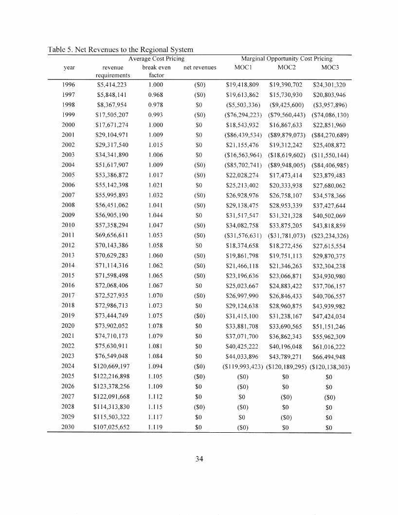
Table 5. Net Revenues to the Regional SystemAverage Cost Pricing Marginal Opportunity Cost Pricing
year revenue break even net revenues MOC1 MOC2 MOC3requirements factor
1996 $5,414,223 1.000 ($0) $19,418,809 $19,390,702 $24,301,320
1997 $5,848,141 0.968 ($0) $19,613,862 $15,730,930 $20,803,946
1998 $8,367,954 0.978 $0 ($5,503,336) ($9,425,600) ($3,957,896)
1999 $17,505,207 0.993 ($0) ($76,294,223) ($79,560,443) ($74,086,130)
2000 $17,671,274 1.000 $0 $18,543,932 $16,867,633 $22,851,960
2001 $29,104,971 1.009 $0 ($86,439,534) ($89,879,073) ($84,270,689)
2002 $29,317,540 1.015 $0 $21,155,476 $19,312,242 $25,408,872
2003 $34,341,890 1.006 $0 ($16,563,964) ($18,619,602) ($11 ,550, 144)
2004 $51,617,907 1.009 ($0) ($85,702,741) ($89,948,005) ($84,406,985)
2005 $53,386,872 1.017 ($0) $22,028,274 $17,473,414 $23,879,483
2006 $55,142,398 1.021 $0 $25,213,402 $20,333,938 $27,680,062
2007 $55,995,893 1.032 ($0) $26,928,976 $26,758,107 $34,578,366
2008 $56,451,062 1.041 ($0) $29,138,475 $28,953,339 $37,427,644
2009 $56,905,190 1.044 $0 $31,517,547 $31,321,328 $40,502,069
2010 $57,358,294 1.047 ($0) $34,082,758 $33,875,205 $43,818,859
2011 $69,656,611 1.053 ($0) ($31,576,631 ) ($31,781,073) ($23,234,326)
2012 $70,143,386 1.058 $0 $18,374,658 $18,272,456 $27,615,554
2013 $70,629,283 1.060 ($0) $19,861,798 $19,751,113 $29,870,375
2014 $71,114,316 1.062 ($0) $21,466,118 $21,346,263 $32,304,238
2015 $71,598,498 1.065 ($0) $23,196,636 $23,066,871 $34,930,980
2016 $72,068,406 1.067 $0 $25,023,667 $24,883,422 $37,706,157
2017 $72,527,935 1.070 ($0) $26,997,990 $26,846,433 $40,706,557
2018 $72,986,713 1.073 $0 $29,124,638 $28,960,875 $43,939,982
2019 $73,444,749 1.075 ($0) $31,415,100 $31,238,167 $47,424,034
2020 $73,902,052 1.078 $0 $33,881,708 $33,690,565 $51,151,246
2021 $74,710,173 1.079 $0 $37,071,700 $36,862,343 $55,962,309
2022 $75,630,911 1.081 $0 $40,425,222 $40,196,048 $61,016,222
2023 $76,549,048 1.084 $0 $44,033,896 $43,789,271 $66,494,948
2024 $120,669,197 1.094 ($0) ($119,993,423) ($120,189,295) ($120,138,303)
2025 $122,216,898 1.105 ($0) ($0) $0 $0
2026 $123,378,256 1.109 $0 ($0) $0 $0
2027 $122,091,668 1.112 $0 $0 ($0) ($0)
2028 $114,313,830 1.115 ($0) ($0) $0 $0
2029 $115,503,322 1.117 $0 $0 ($0) $0
2030 $107,025,652 1.119 $0 ($0) $0 $0
34

Present Value Net Revenues ($1996) ($0) $3,214,902 ($19,485,576) $78,800,757
Table 5 shows that for the MaC rules the surpluses recovered in non-capacity years do
not evenly match deficits in capacity years to generate positive present value net benefits every
case for the planning horizon. To begin, the MOC3 rule generates positive, often rather large,
present value (1996$) net revenues. The surplus revenues are due to the user cost component
which more than offsets any losses due to water use responses to price changes and the lumped
investment bills. Technically, though, the user cost revenues are rents to the state, not
necessarily to the water supplier. Martin et al. note that such excess revenues "could be used to
provide other social services, such as compulsory education, for which society has decided that
the social benefits obviously exceed that private costs" (p. 51). The MOC2 formulation does not
have the user cost component and generates relatively lower revenues with negative present
value net revenues over the planning horizon. The same is true of the MaC 1 formulation,
although, it shows present value net revenues that are positive because environmental mitigation
costs are collected in fixed fees and, thus, do not contribute to price change response induced
revenue losses.
Net Benefits
The analysis of the potential net benefits available from a switch to MOC pricing are
estimated in terms of single family household customers. The net benefits of a move to efficient
MOC pricing are figured as resource or opportunity cost gains (losses) less any losses (gains) in
annual consumer surplus per an average single family household (given by area C in Figure 2).
With this welfare measure, the net community gains per household are greatest where the
estimated MOC efficiency price is significantly higher than the AC price. The simulated price
35

paths show that the difference between AC and MOC is greatest just before (or after) capacity
expansions. Subsequently, the net benefits from pricing reform should be clustered around
(before) capacity expansions.
Figures 4 and 5 summarize the distribution of net benefits available over the planning
horizon from a switch to MOC prices in the study area. The present the net benefits of a discrete
switch in any given year is presented in Figure 4. The net benefits are significant and appear to
peak just before capacity expansions and fall thereafter. Further, the MOC3 formulation offers
the greatest net benefits, followed by MOC2 and MaC 1. These findings alone, however, don't
really suggest much about the "optimal" time to switch to MOC pricing.
Figure 5 shows the present value (year t$) of anticipated total benefits from a permanent
switch to MaC pricing. Net benefits are a maximum at the beginning of the planning horizon in
1996 and decline, with periodic "humps", until 2030. The results imply that the sooner the
switch to MOC pricing the better, but there will continue to be net benefits available throughout
the planning horizon until the backstop technology is in place.
Note that the increase in investment activity at the end of the planning horizon creates
greater present value net benefit opportunities in the latter half of the planning horizon for
MOC 1. This suggests that latter period switches to MOC pricing may be at least as beneficial as
an early switch. The benefits of latter switches, however, should be taken with caution because
as new capacity is accumulated, annual debt service payments will pile-up with AC pricing. The
annual debt service does not disappear with a move to a MaC policy and will have to be
collected somehow, in which case there is pressure to maintain the AC rule. To sum up, where
the switch to MOC pricing is being contemplated and water supply costs are on the rise like in
36

the study area, an earlier switch is preferable to a latter one.
37
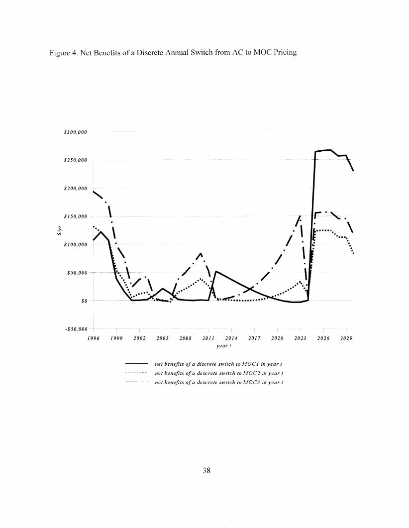
Figure 4. Net Benefits of a Discrete Annual Switch from AC to MOC Pricing
$250,000 -
$200,000
$150,000
$100,000
$50,000 --,.----....~--.----~
j\.-~---
I:. \1- ·
/ \
-$50,000
1996 1999 2002 2005 2008 2011 2014
year t
2017 2020 2023 2026 2029
net benefits of a discrete switch to MOC 1 in year t
net benefits of a descrete switch to MOC 2 in year t
net benefits of a descrete switch to MOC3 in year t
38


Figure 5. Present Value Net Benefits ofa Permanent Switch from AC to MOC Pricing
$1,400,000
$800,000
$1,200,000
$1,000,000
........ .. \...... ........ ~$ 400, 000 --+-~~--------------------::oiIIIIIlIIII""""""=--------~-------- ----- - - - - -------- ---- ----- - _..... ----------- - - - ••- - --- --- -------+-------.--
II •••••• \.. ..... ~........- ..... ... ..... --....... ................._... .~.....
~\
$600,000 ~- . \ ..-- ---. -.~O"'-----~OL---------------------.,.- /
$200,000 --------
$ 0 ---+---------,---------,--------------~------------- --- ------------------------------- ,- ---------
1996 1999 2002 2005 2008 2011 2014 2017 2020 2023 2026 2029year t
PVNB(t) from switch toMDC1 inyeart
PVNB(t) from switch toMDC3 inyeart
PVNB(t) from switch to MDC2 in year t
40
Endnotes
1. In the more usual case where a utility serves more than one customer group (e.g. residential,
commercial, industrial, etc.) with nonuniform (peaking) demand patterns, the portion of shared
debt service cost 'attributable' to each demand service level and customer group and must be
determined. The allocation of costs to customer classes (services), however, is inherently
arbitrary (Baumol, Koehn, and Willig; Braeutigam) due to the prevalence of shared costs in
water service production (Stack 1996).
2. Markets for wholesale water, on the other hand, do appear to be quite responsive to changing
market conditions, though price fluctuations may not accurately reflect changes in resource
values due to externalities, uncertainty and imperfect information. (Saliba et al.).
3. The TVMC formulation produced wild price fluctuations in earlier simulations with the
capacity expansion plan in the present study.
4. A thorough discussion of the AMC and the other marginal capital cost formulations for water
service is found in Russell and Shinn (1996a,b).
5. The external costs can only be considered approximately internalized because mitigation costs
are taken as a proxy to the true external costs that would be revealed with a damage function.
6. This is a fairly accurate characterization where long time horizons are contemplated because
the "used and useful" criterion tends to restrict the amount of "future" costs allowed in current
prices (Deloite and Touche). In shorter time spans (less than two years), however, construction
funds (CWIP) and margin reserve allowances tend to blur timing considerations.
7. This capacity expansion plan represents the anticipated future water supply needs based on a
50% reduction in groundwater pumping phased in at ten percent a year from 1997 and 2007 at
41
all wellfield permits in the region. Further discussion of the wellfield pumping restrictions is
presented in Carter and Milon (1998).
8. See Carter for details on the wholesale-to-retail price conversion
9. The unit cost for backstop water is measured as the predicted total system-wide marginal
operating and environmental cost with the backstop included, which may be more or less than the
marginal operating and environmental cost of the backstop technology alone. This accounts for
the mixing of supply source costs as the marginal costs of the backstop are blended with the rest
of the system costs.
10. Commercial demands were modeled in the study using a constant price elasticity of -.25 and
it was assumed that multi-family residences do not adjust their usage in response to changes in
water prices (Brown and Caldwell in association with John Whitcomb).
11. For the case study, these variables are set to reflect an average household's 1995 base water
use in the study area.
12. The price variable is estimated as the sum of marginal sewer price and a potable water price
that is "ramped" between pricing blocks. The (border) price along the ramp between blocks is
essentially an average of block prices weighted by the portion of consumption (of each
household) occurring within each block. This option provided greater explanatory power than
both average price and marginal price specifications (Brown and Caldwell in association with
John Whitcomb).
13. The details of the aggregation procedure are available in Carter.
14. There were attempts to proxy income which was not available by separating demand and
elasticity estimates for low, medium, and high property values. The initial analysis found
42
differences in elasticities among property values, however, subsequent work (Whitcomb) showed
that these differences are not significant. The medium property value coefficients are used in this
study.
15. The incremental rise in AC prices in the years prior the large capacity expansion in 2002 is
the result of several consecutive smaller capacity increments and is therefore coincidental.
43

References
American Water Works Association (AWWA). Water Rates, Third Edition. Boulder: AWWAManual Ml, 1983.
Baumol, William J., Michael F. Koehn, and Robert D. Willig. "How Arbitrary is "Arbitrary"? or, Toward the Deserved Demise of Full Cost Allocation." Public Utilities Fortnightly123(1987):16-21.
Baumol, William J. and Wallace E. Oates. The Theory ofEnvironmental Policy, Second Edition.Cambridge: Cambridge University Press, 1989.
Beecher, Janice A., Patrick C. Mann, and John R. Landers. Cost Allocation and Rate DesignforWater Utilities. Columbus: The National Regulatory Research Institute, 1990.
Berg, Sanford V. and John Tschirhart. "Contributions of Neoclassical Economics to PublicUtility Analysis." Land Economics 71(1995): 310-330.
Boyle Engineering Corporation. Desalination for Urban Water Supply. Prepared for CaliforniaUrban Water Agencies, 1991.
Boyle Engineering Corporation. WCRWSA Regional Cost Analysis Scenarios A and B. Preparedfor the Southwest Florida Water Management District, 1996.
Brown and Caldwell in association with John B. Whitcomb. Water Price Elasticity Study.Prepared for the Southwest Florida Water Management District, 1993.
Braeutigam, Ronald R. "An Analysis of Fully Distributed Cost Pricing in Regulated Industries."Bell Journal ofEconomics 11 (1980): 182-196.
Carter, David W. Water Supplies and Environmental Externalities: Prospects for Efficient WaterService Pricing in Florida. Master Thesis, Univesity of Florida, Gainesville, 1997.
Ch2MHill. Technical Memorandum E.l.F Wetlands Impact, Mitigation, and Planning-LevelCost Estimating Procedure, Task E: Mitigation and Avoidance ofImpacts. Prepared forthe St. Johns River Water Management District, 1996.
Chesnutt, Thomas W., Casey McSpadden, and John Christianson. "Revenue Instability Inducedby Conservation Rates." Journal ofthe AWWA 88(1996): 52-63.
Crew, M.A. and G. Roberts. "Some Problems of Pricing under Stochastic Supply Conditions:The Case of Seasonal Pricing for Water Supply." Water Resources Research 6(1970):1272-1276.
44

Dandy, G.C., E.A. McBean, and B.G. Hutchinson. "A Model for Constrained Optimum WaterPricing and Capacity Expansion." Water Resources Research 20(1984):511-520.
Dandy, G.C., E.A. McBean, and B.G. Hutchinson. "Pricing and Expansion of a Water SupplySystem." Journal ofWater Resources Planning and Management 111(1985):24-42.
Deloitte and Touche. Public Utilities Manual. Chicago: Deloitte and Touche, 1993.
Feldman, Stephen L., John Breese, and Robert Obeiter. "The Search for Equity and Efficiency inthe Pricing ofa Public Service: Urban Water." Economic Geography 57(1981):78-93.
Freedman, David A. "A Model for Water Pricing." Journal ofBusiness & Economic Statistics4(1986): 131-133.
Goldstein, James. "Full-Cost Water Pricing."Journal ofthe AWWA June(1986):52-61.
Hall, Darwin C. "Calculating Marginal Cost for Water Rates." in Hall, Darwin C. ed. Advancesin the Economics ofEnvironmental Resources, Vol. 1: Marginal cost rate Design andWholesale Water Markets. Greenwich: JAI Press, Inc., 1996.
Hall, Darwin C and W. Michael Hanemann. "Urban Water Rate Design Based on MarginalCost." in Hall, Darwin C. ed. Advances in the Economics ofEnvironmental Resources,Vo!. 1: Marginal cost rate Design and Wholesale Water Markets. Greenwich: JAI Press,Inc., 1996.
Hanke, Steve H. "On Turvey's Benefit-Cost 'Short-Cut': A Study of Water Meters." LandEconomics 58(1982): 144-146.
Hanke, Steve H. "Pricing As A Conservation Tool: An Economist's Dream Come True?" inHoltz, David and Scott Sebastian, eds. Municipal Water Systems: The Challenge forUrban Resources Management. Bloomington: Indiana University Press, 1978.
Hanke, Steve and John Wenders. "Costing and Pricing for Old and New Customers." PublicUtilities Fortnightly 118(1982): 43-47.
Hanemann, W. Michael. "Designing New Water Rates for Los Angeles." Water ResourcesUpdate 92(1993): 11-21.
Heal, Geoffrey M. "The Optimal Use of Exhaustible Resources." in Kneese, A.V. and J.L.Sweeney, eds. Handbook ofNatural Resource and Energy Economics, vol. III NewYork: Elsevier Science Publishers, 1993.
Hirshleifer, J., J. DeHaven and Jerome W. Milliman. Water Supply Economics: Technology and
45

Policy. Chicago: University of Chicago Press, 1960.
Hite, James C. and Holley H. Ulbrich. "Subsidizing Water Users or Water Systems?" LandEconomics 64(1988): 378-380.
Hohmeyer, Olav. Social Costs ofEnergy Consumption: External Effects ofElectricityGeneration in the Federal Republic ofGermany. New York: Springer-Verlag, 1988.
Kim, H.Youn. "Marginal Cost and Second-Best Pricing for Water Services." Review ofIndustrial Organization 10(1995): 323-338.
KPMG Peat Marwick, Governance Study o/The West Coast Regional Water Supply Authority,Draft Report. Prepared for the Florida Legislature, 1996.
Law Environmental in Association with Havens and Emerson, Inc. Water Resource DevelopmentPlan. Prepared for West Coast Regional Water Supply Authority, 1994.
Law Environmental, Expanded Cost Summaries/or the Water Resource Development Plan,Draft. Unpublished, 1994.
LeFrancois, Paul Richard. Average Versus Marginal Cost Pricing/or Water Service. Ph.D.Dissertation, West Virginia University, 1986.
Leggette, Brashears, & Graham, Inc. Estimated Impact ofProposed Regulatory Levels, Draft.Unpublished letter from Frank H. Crum ofL,B,& G, Inc. to William D. Johnson of theCity of St. Petersburg, December, 14, 1995.
Lynne, Gary D. "Scarcity Rents for Water: A Valuation and Pricing Model: Comment." LandEconomics 65(1989):420-424.
Mann, Patrick C. Urban Water Supply: The Divergence Between Theory and Practice. inNowotny, Kenneth, David B. Smith, and Harry M. Trebing, eds. Public UtilityRegulation: Economic and Social Control ofIndustry. Boston: Kulwer AcademicPublishers, 1989.
Mann, Patrick C. and Paul R. Lefrancois. "Trends in the Real Price of Water." Journal o/theAWWA 75(1983):441-443.
Martin, William E., Helen M. Ingram, and Adrian H. Griffin. Saving Water in a Desert City.Washington, D.C.: Resources for the Future, 1984.
McKay, Patricia L., Jerome W. Milliman, and Anne H. Shoemyen. Understanding Impact Fees.Gainesville: Bureau of Economic and Business Research, University of Florida, 1986.
46
Mercer, Lloyd J. and Douglas Morgan. "The Efficiency of Water Pricing: A Rate of ReturnAnalysis for Municipal Water Departments." Water Resources Bulletin 22(1986): 2892950
Moncur, James E.T. and Richard L. Pollock. "Accounting-induced Distortion in PublicEnterprise Pricing." Water Resources Research 32(1996):3355-3360.
Moncur, James E.T. and Richard L. Pollock. "Scarcity Rents for Water: A Valuation and PricingModel: Reply" Land Economics 65(1989):425-428.
Moncur, James E.T. and Richard L. Pollock. "Scarcity Rents for Water: A Valuation and PricingModel." Land Economics 64(1988):62-72.
Munasinghe, Mohan. Managing Water Resources to Avoid Environmental Degradation: PolicyAnalysis and Application. World Bank Environmental Working Paper No. 41, 1990.
Munasinghe, Mohan and Gunter Schramm. Energy Economics, Demand Management andConservation Policy. New York: Van Nostrand Reinhold Company, 1983.
Regional System Water Supply Contract between the West Coast Regional Water SupplyAuthority and the City of St. Petersburg, the City of Tampa, Pasco County, HillsboroughCounty, and Pinellas County, June 7,1991.
Renzetti, Steven. "Evaluating the Welfare Effects of Reforming Municipal Water Prices."Journal ofEnvironmental Economics and Management 22(1992): 147-163.
Riordan, Courtney. "General Multistage Marginal Cost Dynamic Programming Model for theOptimization of a Class of Investment-Pricing Decisions." Water Resources Research7(1971a):245-253.
Riordan, Courtney. "Multistage Marginal Cost Model of Investment-Pricing Decision:Application to Urban Water Supply Treatment Facilities." Water Resources Research7(1971 b):463-478.
Russell, Clifford S. and Boo-Shig Shin. "Public Utility Pricing: Theory and PracticalLimitations." in Hall, Darwin C. ed. Advances in the Economics ofEnvironmentalResources, Vol. 1: Marginal Cost Rate Design and Wholesale Water Markets.Greenwich: JAI Press, Inc., 1996a.
Russell, Clifford S. and Boo-Shig Shin. "An Application and Evaluation of Competing MarginalCost Approximations." in Hall, Darwin C. ed. Advances in the Economics ofEnvironmental Resources, Vol. 1: Marginal Cost Rate Design and Wholesale Water
47

Markets. Greenwich: JAI Press, Inc., 1996b.
Saliba, Bonnie, David B. Bush, William E. Martin, and Thomas C. Brown. "Do Water MarketPrices Appropriately Measure Water Values?" Natural Resources Journal 27(1987):617651.
Saunders, Robert J., Jeremy J. Warford, and Patrick C. Mann. Alternative Concepts ofMarginalCost for Public Utility Pricing: Problems ofApplication in the Water Supply Sector.International Bank for Reconstruction and Development Staff Working Paper 259, 1977.
Schramm, Gunter. "Practical Approaches for Estimating Resource Depletion Costs." in Miles,E., R. Pealy, and R. Stokes, eds. Natural Resource Economics and Policy Applications:Essays in Honor ofJames A. Crutchfield. University of Washington Press, 1986.
Serrano, Laura. and Luis. Serrano. "Influence of Groundwater Exploitation for Urban WaterSupply on Temporary Ponds from the Donana National State Park (SW Spain)." JournalofEnvironmental Management 46(1996):229-238.
Southwest Florida Water Management District (SWFWMD). Northern Tampa Bay WaterResource Assessment Project. Brooksville: SWFWMD, 1994.
Stack, Thomas R. "Water Cost of Service Studies." Presented at the 24th Annual Eastern UtilityRate Seminar, Clearwater, FI, 1996.
Swallow, Stephen K. and Carlos M. Marin. "Long Run Price Inflexibility and Efficiency Loss forMunicipal Water Supply." Journal ofEnvironmental Economics and Management15(1988):233-247.
Thomas, J.F. and W.E. Martin. "Mining of Aquifers Near Metropolitan Areas: Towards aGeneral Framework for Policy Analysis." in Custodio, E. and A. Gurgui, eds.Groundwater Economics. New York: Elsevier, 1989.
Warford, Jeremy J. Marginal Opportunity Cost Pricingfor Municipal Water Supply. EEPSEADiscussion Paper on Water Pricing, 1996.
Whitcomb, John B. Single Family Price Elasticity Recalculation. Unpublished memo to JayYingling, Senior Economist at the Southwest Florida Water Management District, 1995.
Williamson, Oliver E. "Peak-Load Pricing and Optimal Capacity Under IndivisibilityConstraints." The American Economic Review 56(4, Part 1)(1966):81 0-827.
48


