Download - Machine learning: a probabilistic approachmurphyk/Teaching/CS340-Fall06/lectures/review-4pp.pdfCS340: Machine Learning Review for midterm Kevin Murphy Machine learning: a probabilistic

CS340: Machine Learning

Review for midterm

Kevin Murphy

Machine learning: a probabilistic approach

•We want to make models of data so we can find patterns andpredict the future.

•We will use probability theory to represent our uncertainty aboutwhat the right model is; this will induce uncertainty in ourpredictions.

•We will update our beliefs about the model as we acquire data (thisis called “learning”); as we get more data, the uncertainty in ourpredictions will decrease.

Outline

• Probability basics

• Probability density functions

• Parameter estimation

• Prediction

•Multivariate probability models

• Conditional probability models

• Information theory

Probability basics

• Chain (product) rule

p(A,B) = p(A)p(B|A) (1)

•Marginalization (sum) rule

p(B) =∑

a

p(A = a,B) (2)

• Hence we derive Bayes rule

p(A|B) =p(A,B)

p(B)(3)

PMF

• A probability mass function (PMF) is defined on a discrete randomvariable X ∈ {1, . . . ,K} and satisfies

1 =

K∑

x=1

P (X = x) (4)

0 ≤ P (X = x) ≤ 1 (5)

• This is just a histogram!

PDF

• A probability density function (PDF) is defined on a continuousrandom variable X ∈ IR or X ∈ IR+ or X ∈ [0, 1] etc and satisfies

1 =

∫

Xp(X = x)dx (6)

0 ≤ p(X = x) (7)

• Note that it is possible that p(X = x) > 1, since multiplied by dx.

• P (x ≤ X ≤ x + dx) ≈ p(x)dx

• Statistics books often write fX(x) for pdfs and use P () for pmf’s.

Moments of a distribution

•Mean (first central moment)

µ = E[X ] =∑

x

xp(x) (8)

• Variance (second central moment)

σ2 = Var [X ] =∑

x

(x − µ)2p(x) = E[X2] − µ2 (9)

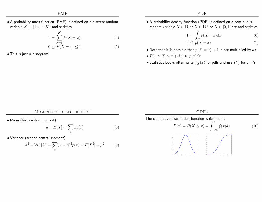
CDFs

The cumulative distribution function is defined as

F (x) = P (X ≤ x) =

∫ x

−∞f (x)dx (10)

−3 −2 −1 0 1 2 30

0.05

0.1

0.15

0.2

0.25

0.3

0.35

0.4

x

p(x)

Standard Normal

−3 −2 −1 0 1 2 30

0.1

0.2

0.3

0.4

0.5

0.6

0.7

0.8

0.9

1

x

p(x)

Gaussian cdf

Quantiles of a distribution

P (a ≤ X ≤ b) = FX(b) − FX(a) (11)

eg if Z ∼ N (0, 1), FZ(z) = Φ(z). Then

p(−1.96 ≤ Z ≤ 1.96) = Φ(1.96) − Φ(−1.96) (12)

= 0.975 − 0.025 = 0.95 (13)

Hence X ∼ N (µ, σ),

p(−1.96σ < X − µ < 1.96σ) = 1 − 2 × 0.025 = 0.95 (14)

Hence the interval µ ± 1.96σ contains 0.95 mass.

Outline

• Probability basics√

• Probability density functions


• Prediction




Bernoulli distribution

•X ∈ {0, 1}, p(X = 1) = θ, p(X = 0) = 1 − θ

•X ∼ Be(θ)

•E[X ] = θ

Multinomial distribution

•X ∈ {1, . . . ,K}, p(X = k) = θk, X ∼ Mu(θ)

• 0 ≤ θk ≤ 1

•∑Kk=1 θk = 1

•E[Xi] = θi

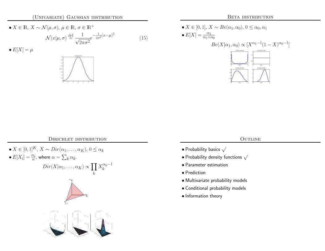
(Univariate) Gaussian distribution

•X ∈ IR, X ∼ N (µ, σ), µ ∈ IR, σ ∈ IR+

N (x|µ, σ)def=

1√2πσ2

e− 1

2σ2(x−µ)2(15)

•E[X ] = µ

−3 −2 −1 0 1 2 30

0.05

0.1

0.15

0.2

0.25

0.3

0.35

0.4

x

p(x)

Standard Normal

Beta distribution

•X ∈ [0, 1], X ∼ Be(α1, α0), 0 ≤ α0, α1

•E[X ] = α1α1+α0

Be(X|α1, α0) ∝ [Xα1−1(1 − X)α0−1]

0 0.5 10

1

2

3

4a=0.10, b=0.10

0 0.5 10

0.5

1

1.5

2a=1.00, b=1.00

0 0.5 10

0.5

1

1.5

2a=2.00, b=3.00

0 0.5 10

1

2

3a=8.00, b=4.00

Dirichlet distribution

•X ∈ [0, 1]K, X ∼ Dir(α1, . . . , αK), 0 ≤ αk

•E[Xi] = αiα , where α =

∑

k αk.

Dir(X|α1, . . . , αK) ∝∏

k

Xαk−1k

Outline


• Probability density functions√


• Prediction




Parameter estimation: MLE

• Likelihood of iid data D = {xn}Nn=1

L(θ) = p(D|θ) =∏

n

p(xn|θ) (16)

• Log likelihood

`(θ) = log p(D|θ) =∑

n

log p(xn|θ) (17)

•MLE = Maximum likelihood estimate

θ = arg maxθ

L(θ) = arg maxθ

`(θ) (18)

hence∂L

∂θi= 0 (19)

MLE for Bernoullis

p(Xn|θ) = θXn(1 − θ)1−Xn (20)

`(θ) =∑

n

Xn log θ +∑

n

(1 − Xn) log(1 − θ) (21)

= N1 log θ + N0 log(1 − θ) (22)

N1 =∑

n

I(Xn = 1) (23)

dL

dθ=

N1

θ− N0

1 − θ= 0 (24)

θ =N1

N1 + N0(25)

MLE for Multinomials

p(Xn|θ) =∏

k

θI(Xn=k)k

(26)

`(θ) =∑

n

∑

k

I(xn = k) log θk (27)

=∑

k

Nk log θk (28)

l =∑

k

Nk log θk + λ

1 −∑

k

θk

(29)

∂l

∂θk=

Nk

θk− λ = 0 (30)

θk =Nk

N(31)

Parameter estimation: Bayesian

p(θ|D) ∝ p(D|θ)p(θ) (32)

= [∏

n

p(xn|θ)]p(θ) (33)

We say p(θ) is conjugate to p(D|θ) if p(θ|D) in same family as p(θ).This allows recursive (sequential) updating.MLE is a point estimate. Bayes computes full posterior, natural modelof uncertainty (e.g., posterior variance, entropy, credible intervals, etc)

Parameter estimation: MAP

For many models, as |D|→∞,

p(θ|D)→δ(θ − θMAP )→δ(θ − θMLE) (34)

whereθMAP = arg max

θp(D|θ)p(θ) (35)

MAP (maximum a posteriori) estimate is a posterior mode. Also calleda penalized likelihood estimate since

θMAP = arg maxθ

log p(D|θ) − λc(θ) (36)

where c(θ) = − log p(θ) is a penalty or regularizer, and λ is thestrenghth of the regularizer.

Bayes estimate for Bernoulli

Xn ∼ Be(θ) (37)

θ ∼ Beta(α1, α0) (38)

p(θ|D) ∝ [∏

n

θXn(1 − θ)1−Xn]θα1−1(1 − θ)α0−1 (39)

= θN1(1 − θ)N0θα1−1(1 − θ)α0−1 (40)

∝ Beta(α1 + N1, α0 + N0) (41)

Bayes estimate for Multinomial

Xn ∼ Mu(θ) (42)

θ ∼ Dir(α1, . . . , αK) (43)

p(θ|D) ∝ [∏

n

∏

k

θI(Xn=k)k

]∏

k

θαk−1k

(44)

=∏

k

θNkk

θαk−1k

(45)

∝ Dir(α1 + N1, . . . , αK + NK) (46)

Outline



• Parameter estimation√

• Prediction




Multivariate probability models

• Each data case Xn is now a vector of variables Xni, i = 1 : p,n = 1 : N

• e.g., Xni ∈ {1, . . . ,K} is the i’th word in n’th sentence

• e.g., Xni ∈ IR is the i’th attribute in the n’th feature vector

•We need to define p(Xn|θ) for feature vectors of potentially variablesize.

Independent features (bag of words model)

p(Xn|θ) =∏

i

p(Xni|θi) (55)

e.g., Xni ∈ {0, 1}, product of Bernoullis

p(Xn|θ) =∏

i

θXnii (1 − θi)

Xni (56)

e.g., Xni ∈ {1, . . . ,K}, product of multinomials

p(Xn|θ) =∏

i

∏

k

θI(Xni=k)ik

(57)

MLE for bag of words model

p(D|θ) =∏

n

∏

i

p(Xni|θi) (58)

We can estimate each θi separately, eg. product of multinomials

p(D|θ) =∏

n

∏

i

∏

k

θI(Xni=k)ik

(59)

=∏

i

∏

k

θNikik

(60)

Nikdef=

∑

n

I(Xni = k) (61)

`(θi) =∑

k

Nik log θik (62)

θik =Nik

Ni(63)

Bayes estimate for bag of words model

p(θ|D) ∝∏

i

p(θi)[∏

n

∏

i

p(Xni|θi)] (64)

We can update each θi separately, eg. product of multinomials

p(θ|D) =∏

i

Dir(θi|αi1, . . . , αiK)[∏

k

θNikik

] (65)

∝∏

i

Dir(θi|αi1 + Ni1, . . . , αiK + NiK) (66)

Factored prior × factored likelihood = factored posterior

(Discrete time) Markov model

p(Xn|θ) = p(Xn1|π)

p∏

t=2

p(Xnt|Xn,t−1, A) (67)

For a discrete state space, Xnt ∈ {1, . . . ,K},πi = p(X1 = i) (68)

Aij = p(Xt = j|Xt−1 = i) (69)

p(Xn|θ) =∏

i

πI(Xn1=i)i

∏

t

∏

i

∏

j

AI(Xnt=j,Xn,t−1=i)ij (70)

=∏

i

πN1

ii

∏

i

∏

j

ANij

ij (71)

N1i

def= I(Xn1 = i) (72)

Nijdef=

∑

t

I(Xn,t = j,Xn,t−1 = i) (73)

MLE for Markov model

p(D|θ) =∏

n

∏

i

πI(Xn1=i)i

∏

t

∏

i

∏

j

AI(Xnt=j,Xn,t−1=i)ij (74)

=∏

i

πN1

ii

∏

i

∏

j

ANij

ij (75)

N1i

def=

∑

n

I(Xn1 = i) (76)

Nijdef=

∑

n

∑

t

I(Xn,t = j,Xn,t−1 = i) (77)

Aij =Nij

∑

j′ Nij′(78)

πi =N1

i

N(79)

Stationary distribution for a Markov chain

πi is fraction of time we spend in state i, given by principle eigenvector

Aπ = π (80)

Balance flow across cut set

π1α = π2β (81)

Since π1 + π2 = 1, we have

π1 =β

α + β, π2 =

α

α + β, (82)

Outline




• Prediction√

•Multivariate probability models√



Conditional density estimation

• Goal: learn p(y|x) where x is input and y is output.

• Generative modelp(y|x) ∝ p(x|y)p(y) (83)

•Discriminative model e.g., logistic regression

p(y|x) = σ(wTx) (84)

Naive Bayes = conditional bag of words model

Generative modelp(y|x) ∝ p(x|y)p(y) (85)

in which features of x are conditionally independent given y:

p(y|x) ∝ p(y)[

p∏

i=1

p(xi|y)] (86)

e.g., for multinomials

p(y|x) ∝∏

c

πI(y=c)c [

∏

i

∏

k

θI(xi=k,y=c)cik

] (87)

MLE for Naive Bayes

We estimate params for each feature separately, partitioning the databased on label y.

p(D|θ, π) = [∏

c

πNcc ]

∏

i

[∏

k

∏

c

θNcikcik

] (88)

Ncik =∑

n

I(xni = k, yn = c) (89)

θcik =Ncik

∑

k′ Ncik′(90)

πc =Nc

N(91)

Conditional Markov model

p(x|y) = p(x1|y)∏

t

p(xt|xt−1, y) (92)

Fit a separate Markov model for every class of y. See homework 5.

Summary Summary

• Probability basics: Bayes rule, pdfs, pmfs

• Probability density functions: Bernoulli, Multinomial; Gaussian,Beta, Dirichlet

• Parameter estimation: MLE, Bayesian

• Prediction: Plug-in, Bayesian, cross validation

•Multivariate probability models: Bag of words, Markov models

• Conditional probability models: Conditional BOW (Naive Bayes),Conditional Markov


Entropy

•Measure of uncertainty.

•Definition for PMF pk, k = 1 : K

H(p) = −∑

k

pk log2 pk (93)

• eg binary entropy function, p1 = θ, p0 = 1 − θ

H(θ) = −[p(X = 1) log2 p(X = 1) + p(X = 0) log2 p(X = 0)](94)

= −[θ log2 θ + (1 − θ) log2(1 − θ)] (95)

Joint entropy

H(X,Y ) = −∑

x,y

p(x, y) log p(x, y) (96)

If X ⊥ Y , then H(X,Y ) = H(X) + H(Y ).Pf:

H(X,Y ) = −∑

x,y

p(x)p(y) log p(x)p(y) (97)

= −∑

x,y

p(x)p(y) log p(x) −∑

x,y

p(x)p(y) log p(y) (98)

In generalH(X,Y ) ≤ H(X) + H(Y ) (99)

Pf:I(X,Y ) = H(X) + H(Y ) − H(X,Y ) ≥ 0 (100)

Conditional entropy

H(Y |X)def=

∑

x

p(x)H(Y |X = x) (101)

= H(X,Y ) − H(X) (102)

In hw 5, you showed that H(Y |X) ≤ H(Y ).Pf

H(Y |X) = H(X,Y ) − H(X) ≤ H(X) + H(Y ) − H(Y ) (103)

But ∃y.H(X|y) > H(X).

Mutual information

I(X ; Y ) =∑

y∈Y

∑

x∈X

p(x, y) logp(x, y)

p(x) p(y)(104)

In hw 5, you showed that

I(X,Y ) = H(X) − H(X|Y ) = H(Y ) − H(Y |X) (105)

Subsituting H(Y |X) = H(X,Y ) − H(X) yields

I(X,Y ) = H(X) + H(Y ) − H(X,Y ) (106)

Mutual information ≥ 0

I(X,Y ) = 0 if X ⊥ Y . Pf.

I(X ; Y ) =∑

y∈Y

∑

x∈X

p(x)p(y) logp(x)p(y)

p(x) p(y)(107)

=∑

y

∑

x

p(x)p(y) log 1 = 0 (108)

I(X,Y ) ≥ 0. Pf.

I(X,Y ) = KL(p(x, y)||p(x)p(y)) ≥ 0 (109)

Relative entropy

D(p||q)def=

∑

k

pk logpk

qk(110)

=∑

k

pk log pk −∑

k

pk log qk (111)

= −∑

k

pk log qk − H(p) (112)

Hence measures extra number of bits needed to encode data if we useq instead of p.D(p||q) = 0 if p = q. Pf: trivial.D(p||q) ≥ 0. Pf: use Jensen’s inequality.

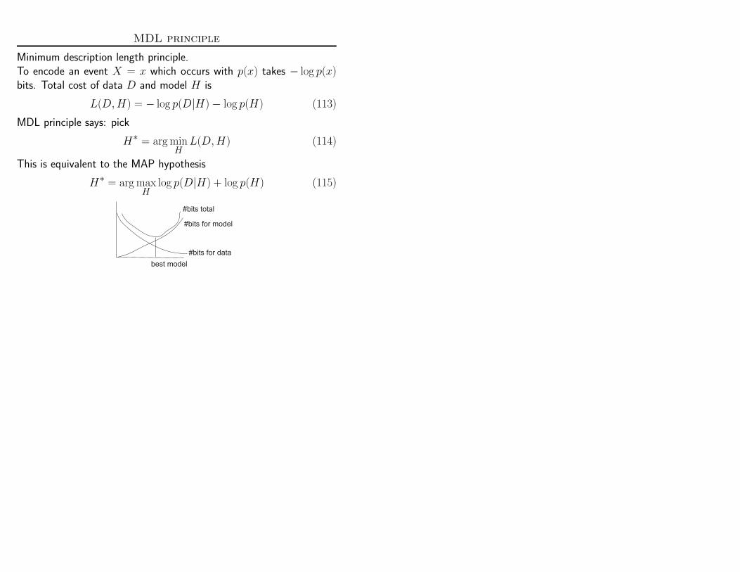
MDL principle

Minimum description length principle.To encode an event X = x which occurs with p(x) takes − log p(x)bits. Total cost of data D and model H is

L(D,H) = − log p(D|H) − log p(H) (113)

MDL principle says: pick

H∗ = arg minH

L(D,H) (114)

This is equivalent to the MAP hypothesis

H∗ = arg maxH

log p(D|H) + log p(H) (115)

#bits for data

#bits for model

#bits total

best model

Download - Machine learning: a probabilistic approachmurphyk/Teaching/CS340-Fall06/lectures/review-4pp.pdfCS340: Machine Learning Review for midterm Kevin Murphy Machine learning: a probabilistic

Top Related