
L. Vandenberghe EE236C (Spring 2016)
4. Subgradients
• definition
• subgradient calculus
• duality and optimality conditions
• directional derivative
4-1
Basic inequality
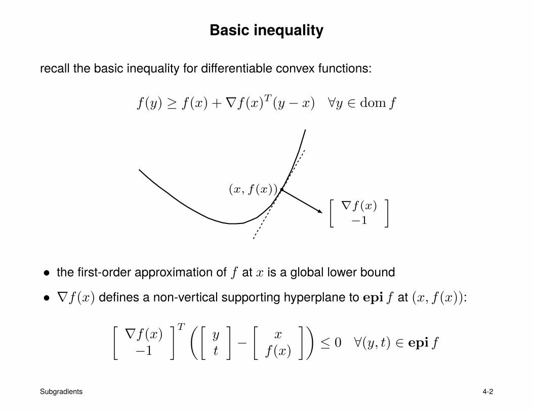
recall the basic inequality for differentiable convex functions:
f(y) ≥ f(x) +∇f(x)T (y − x) ∀y ∈ dom f
(x, f(x)) [ ∇f(x)
−1
]
• the first-order approximation of f at x is a global lower bound
• ∇f(x) defines a non-vertical supporting hyperplane to epi f at (x, f(x)):[∇f(x)−1
]T ([yt
]−[
xf(x)
])≤ 0 ∀(y, t) ∈ epi f
Subgradients 4-2
Subgradient
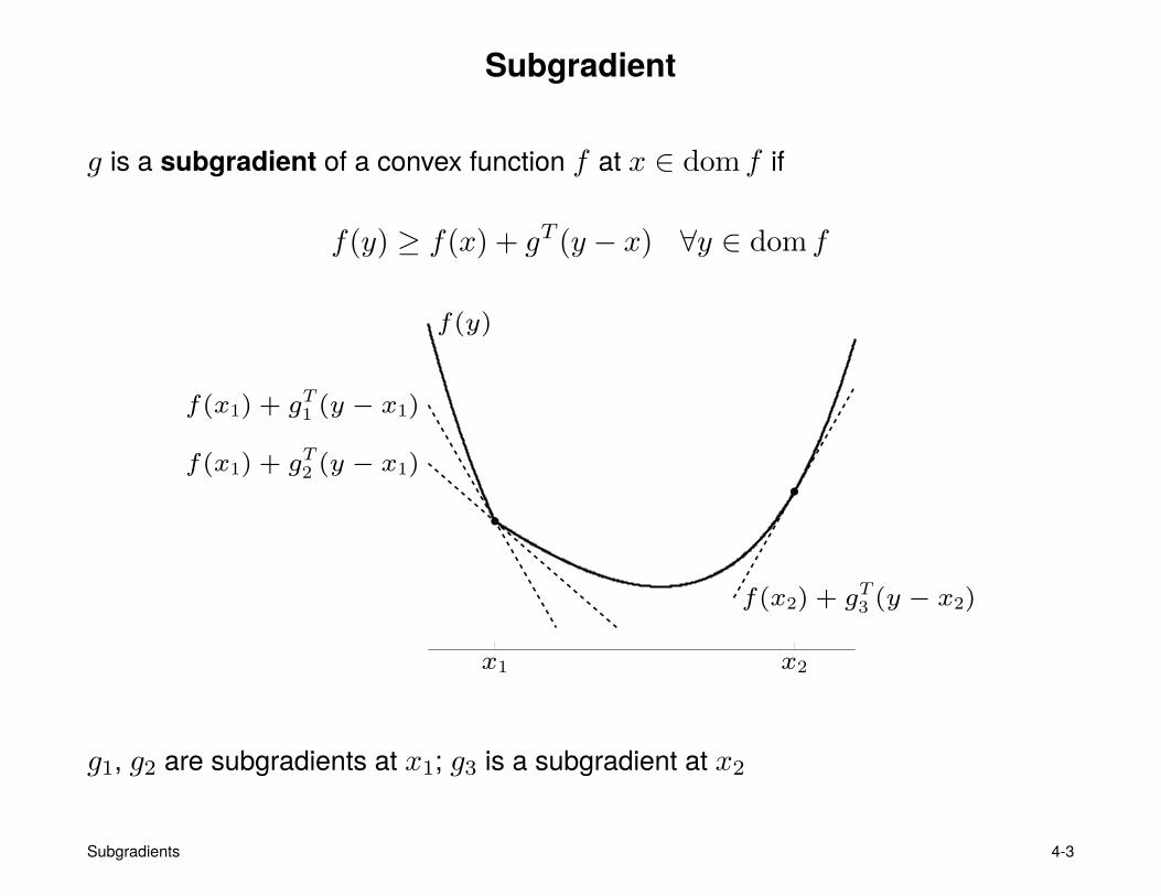
g is a subgradient of a convex function f at x ∈ dom f if
f(y) ≥ f(x) + gT (y − x) ∀y ∈ dom f
x1 x2
f(y)
f(x1) + gT1 (y − x1)
f(x1) + gT2 (y − x1)
f(x2) + gT3 (y − x2)
g1, g2 are subgradients at x1; g3 is a subgradient at x2
Subgradients 4-3

Subdifferential
the subdifferential ∂f(x) of f at x is the set of all subgradients:
∂f(x) = {g | gT (y − x) ≤ f(y)− f(x), ∀y ∈ dom f}
Properties
• ∂f(x) is a closed convex set (possibly empty)
this follows from the definition: ∂f(x) is an intersection of halfspaces
• if x ∈ int dom f then ∂f(x) is nonempty and bounded
proof on next two pages
Subgradients 4-4
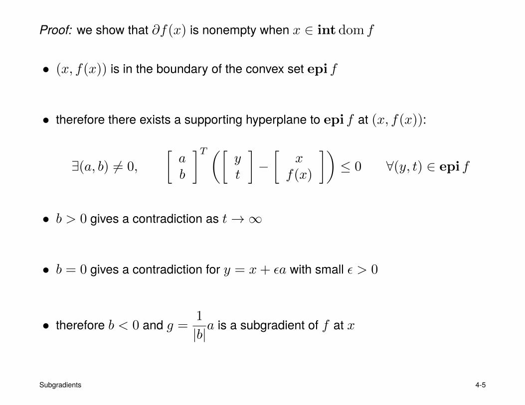
Proof: we show that ∂f(x) is nonempty when x ∈ int dom f
• (x, f(x)) is in the boundary of the convex set epi f
• therefore there exists a supporting hyperplane to epi f at (x, f(x)):
∃(a, b) 6= 0,
[ab
]T ([yt
]−[
xf(x)
])≤ 0 ∀(y, t) ∈ epi f
• b > 0 gives a contradiction as t→∞
• b = 0 gives a contradiction for y = x+ εa with small ε > 0
• therefore b < 0 and g =1
|b|a is a subgradient of f at x
Subgradients 4-5
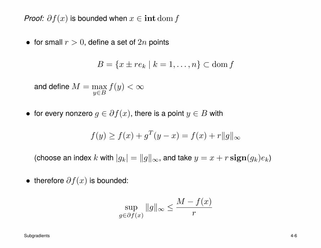
Proof: ∂f(x) is bounded when x ∈ int dom f
• for small r > 0, define a set of 2n points
B = {x± rek | k = 1, . . . , n} ⊂ dom f
and defineM = maxy∈B
f(y) <∞
• for every nonzero g ∈ ∂f(x), there is a point y ∈ B with
f(y) ≥ f(x) + gT (y − x) = f(x) + r‖g‖∞
(choose an index k with |gk| = ‖g‖∞, and take y = x+ r sign(gk)ek)
• therefore ∂f(x) is bounded:
supg∈∂f(x)
‖g‖∞ ≤M − f(x)
r
Subgradients 4-6
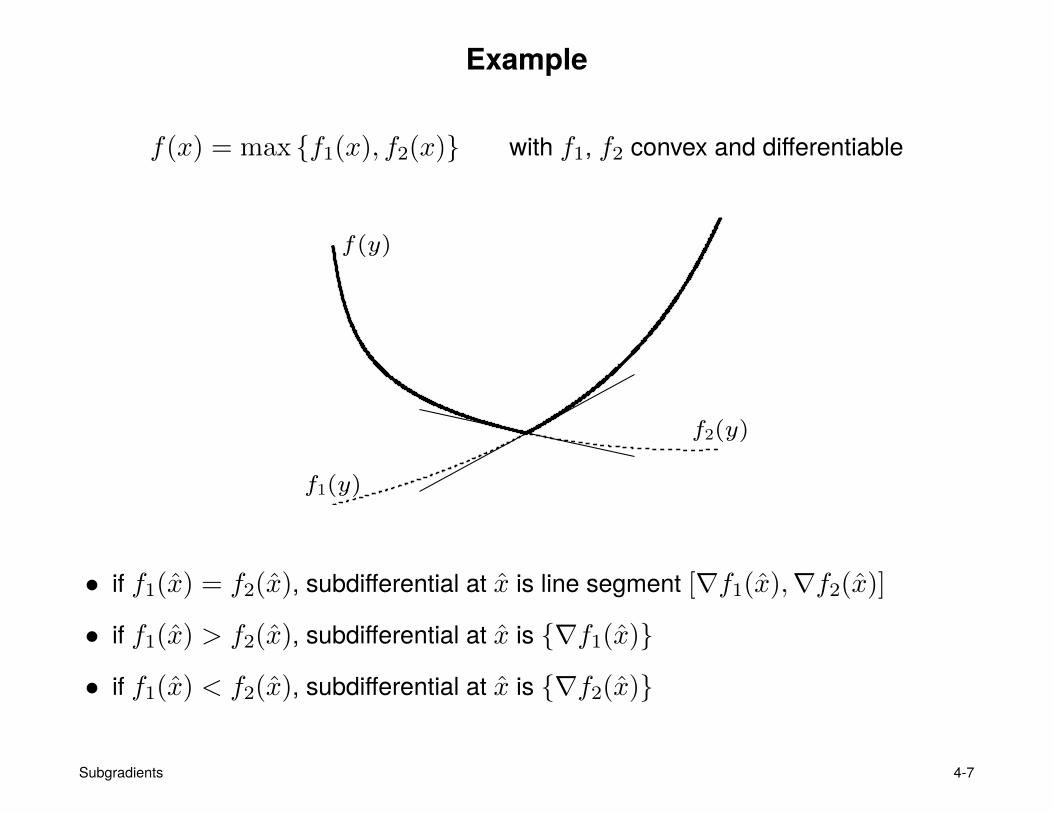
Example
f(x) = max {f1(x), f2(x)} with f1, f2 convex and differentiable
f(y)
f1(y)
f2(y)
• if f1(x) = f2(x), subdifferential at x is line segment [∇f1(x),∇f2(x)]
• if f1(x) > f2(x), subdifferential at x is {∇f1(x)}
• if f1(x) < f2(x), subdifferential at x is {∇f2(x)}
Subgradients 4-7
Examples
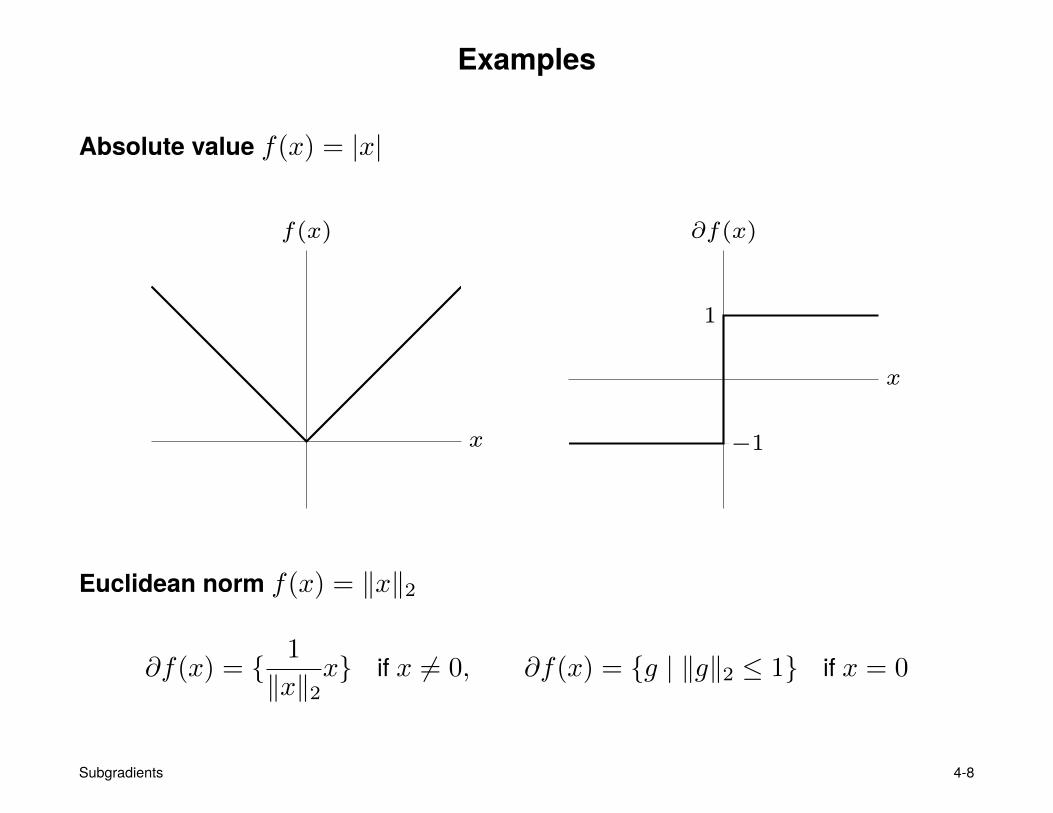
Absolute value f(x) = |x|
x
f(x)
1
−1
x
∂f(x)
Euclidean norm f(x) = ‖x‖2
∂f(x) = { 1
‖x‖2x} if x 6= 0, ∂f(x) = {g | ‖g‖2 ≤ 1} if x = 0
Subgradients 4-8

Monotonicity
the subdifferential of a convex function is a monotone operator:
(u− v)T (x− y) ≥ 0 ∀x, y, u ∈ ∂f(x), v ∈ ∂f(y)
Proof: by definition
f(y) ≥ f(x) + uT (y − x), f(x) ≥ f(y) + vT (x− y)
combining the two inequalities shows monotonicity
Subgradients 4-9

Examples of non-subdifferentiable functions
the following functions are not subdifferentiable at x = 0
• f : R→ R, dom f = R+
f(x) = 1 if x = 0, f(x) = 0 if x > 0
• f : R→ R, dom f = R+
f(x) = −√x
the only supporting hyperplane to epi f at (0, f(0)) is vertical
Subgradients 4-10
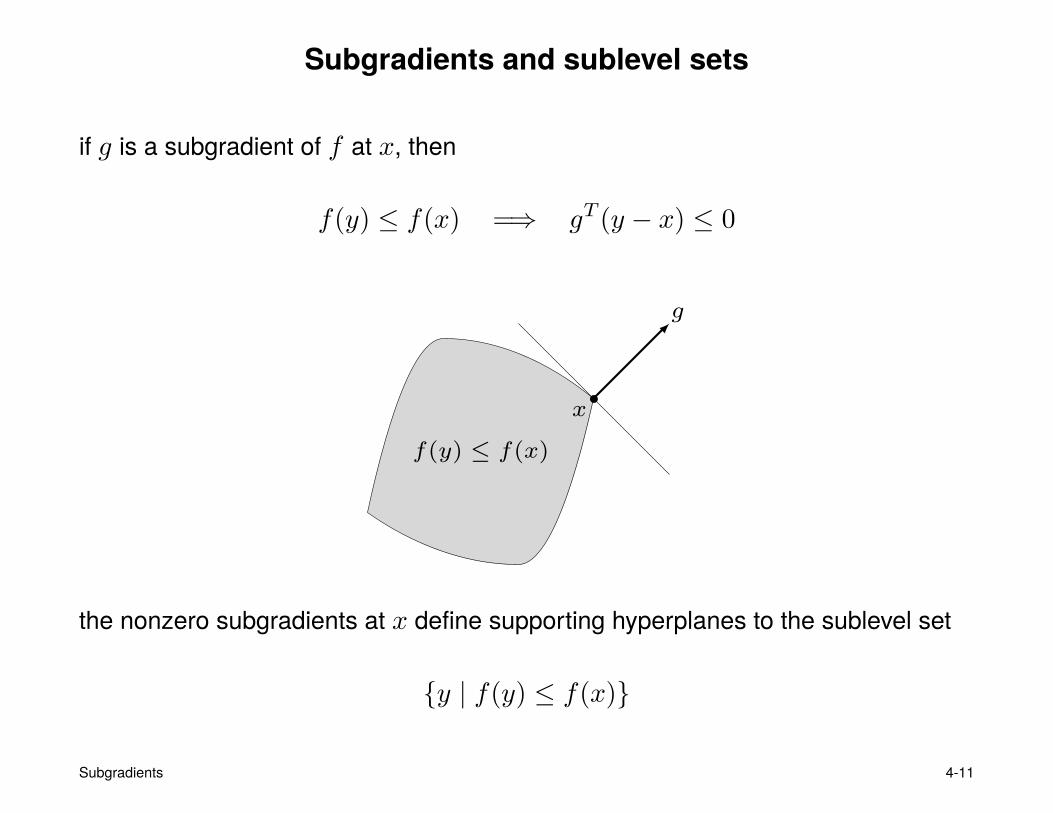
Subgradients and sublevel sets
if g is a subgradient of f at x, then
f(y) ≤ f(x) =⇒ gT (y − x) ≤ 0
f(y) ≤ f(x)
x
g
the nonzero subgradients at x define supporting hyperplanes to the sublevel set
{y | f(y) ≤ f(x)}
Subgradients 4-11
Outline
• definition
• subgradient calculus
• duality and optimality conditions
• directional derivative
Subgradient calculus
Weak subgradient calculus: rules for finding one subgradient
• sufficient for most nondifferentiable convex optimization algorithms
• if you can evaluate f(x), you can usually compute a subgradient
Strong subgradient calculus: rules for finding ∂f(x) (all subgradients)
• some algorithms, optimality conditions, etc., need entire subdifferential
• can be quite complicated
we will assume that x ∈ int dom f
Subgradients 4-12
Basic rules
Differentiable functions: ∂f(x) = {∇f(x)} if f is differentiable at x
Nonnegative linear combination
if f(x) = α1f1(x) + α2f2(x) with α1, α2 ≥ 0, then
∂f(x) = α1∂f1(x) + α2∂f2(x)
(r.h.s. is addition of sets)
Affine transformation of variables: if f(x) = h(Ax+ b), then
∂f(x) = AT∂h(Ax+ b)
Subgradients 4-13
Pointwise maximum
f(x) = max {f1(x), . . . , fm(x)}
define I(x) = {i | fi(x) = f(x)}, the ‘active’ functions at x
Weak result:
to compute a subgradient at x, choose any k ∈ I(x), any subgradient of fk at x
Strong result∂f(x) = conv
⋃i∈I(x)
∂fi(x)
• the convex hull of the union of subdifferentials of ‘active’ functions at x
• if fi’s are differentiable, ∂f(x) = conv {∇fi(x) | i ∈ I(x)}
Subgradients 4-14
Example: piecewise-linear function
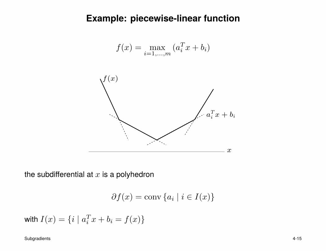
f(x) = maxi=1,...,m
(aTi x+ bi)
f(x)
aTi x + bi
x
the subdifferential at x is a polyhedron
∂f(x) = conv {ai | i ∈ I(x)}
with I(x) = {i | aTi x+ bi = f(x)}
Subgradients 4-15
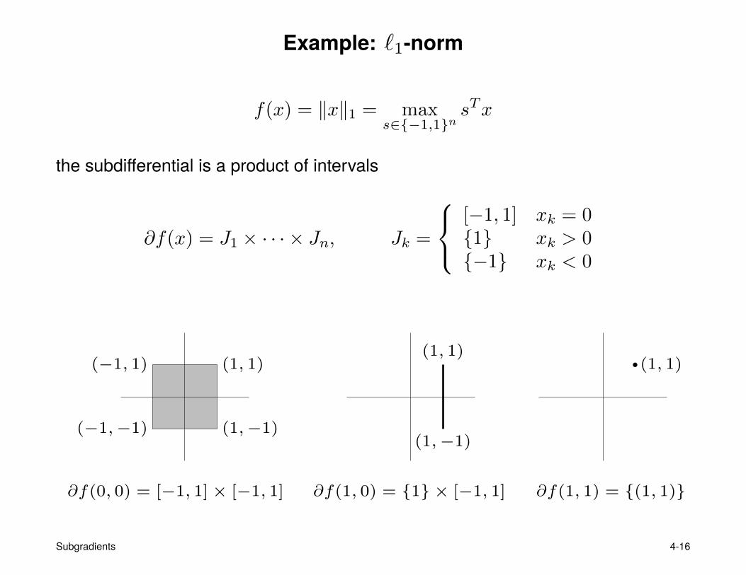
Example: `1-norm
f(x) = ‖x‖1 = maxs∈{−1,1}n
sTx
the subdifferential is a product of intervals
∂f(x) = J1 × · · · × Jn, Jk =
[−1, 1] xk = 0{1} xk > 0{−1} xk < 0
(1, 1)(−1, 1)
(−1,−1) (1,−1)
(1, 1)
(1,−1)
(1, 1)
∂f(0, 0) = [−1, 1]× [−1, 1] ∂f(1, 0) = {1} × [−1, 1] ∂f(1, 1) = {(1, 1)}
Subgradients 4-16
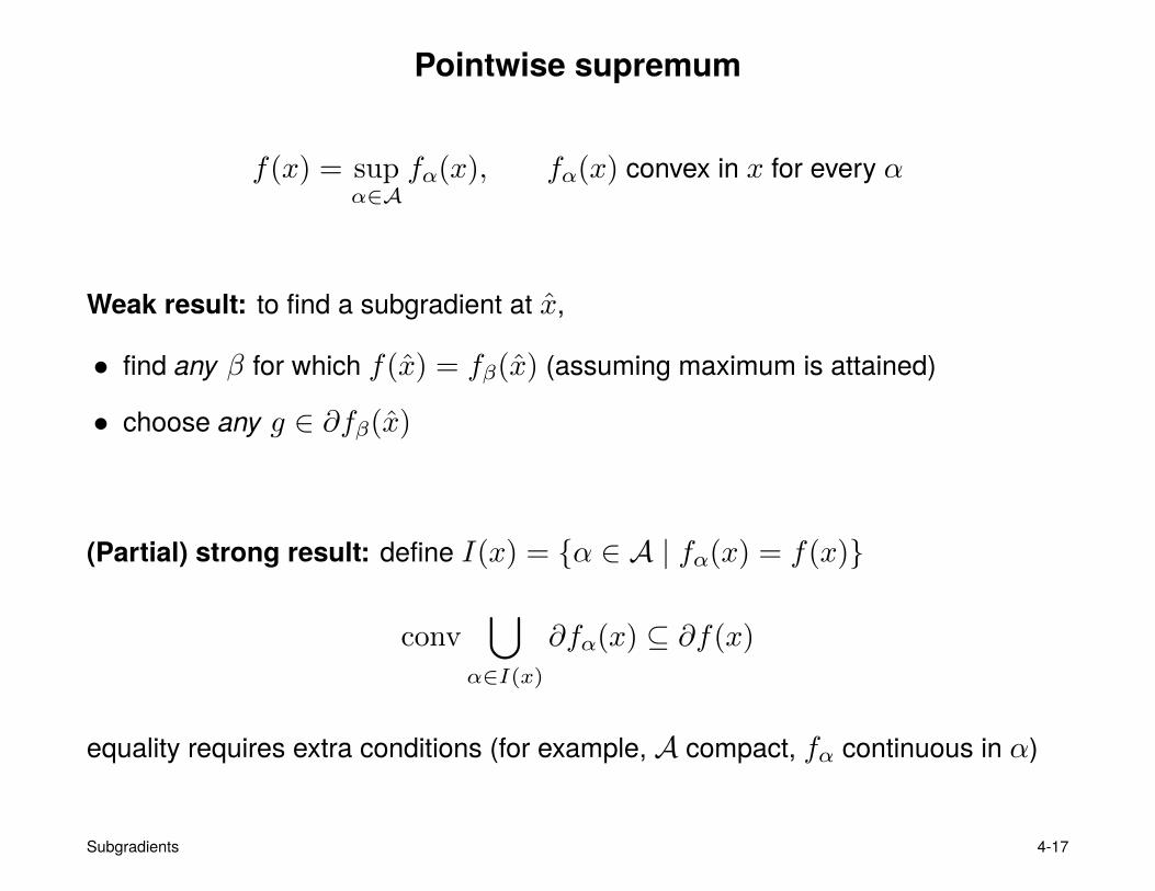
Pointwise supremum
f(x) = supα∈A
fα(x), fα(x) convex in x for every α
Weak result: to find a subgradient at x,
• find any β for which f(x) = fβ(x) (assuming maximum is attained)
• choose any g ∈ ∂fβ(x)
(Partial) strong result: define I(x) = {α ∈ A | fα(x) = f(x)}
conv⋃
α∈I(x)∂fα(x) ⊆ ∂f(x)
equality requires extra conditions (for example, A compact, fα continuous in α)
Subgradients 4-17
Exercise: maximum eigenvalue
Problem: explain how to find a subgradient of
f(x) = λmax(A(x)) = sup‖y‖2=1
yTA(x)y
where A(x) = A0 + x1A1 + · · ·+ xnAn with symmetric coefficients Ai
Solution: to find a subgradient at x,
• choose any unit eigenvector y with eigenvalue λmax(A(x))
• the gradient of yTA(x)y at x is a subgradient of f :
(yTA1y, . . . , yTAny) ∈ ∂f(x)
Subgradients 4-18
Minimization
f(x) = infyh(x, y), h jointly convex in (x, y)
Weak result: to find a subgradient at x,
• find y that minimizes h(x, y) (assuming minimum is attained)
• find subgradient (g, 0) ∈ ∂h(x, y)
Proof: for all x, y,
h(x, y) ≥ h(x, y) + gT (x− x) + 0T (y − y)
= f(x) + gT (x− x)
thereforef(x) = inf
yh(x, y) ≥ f(x) + gT (x− x)
Subgradients 4-19
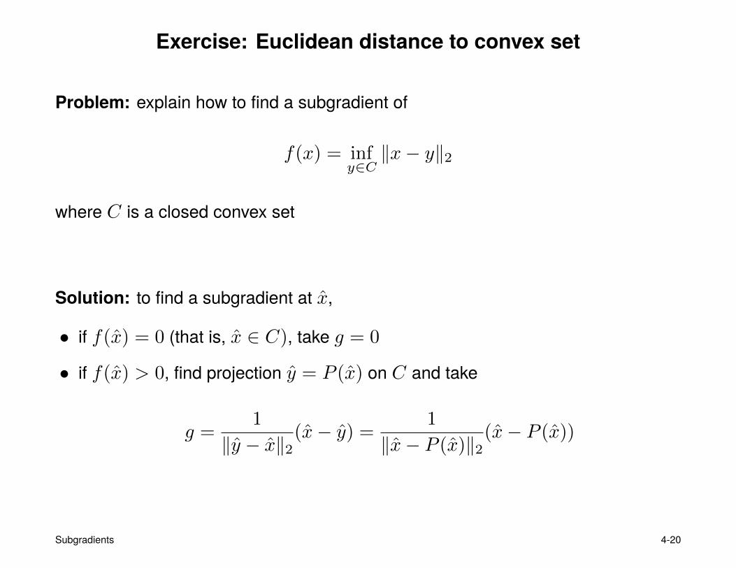
Exercise: Euclidean distance to convex set
Problem: explain how to find a subgradient of
f(x) = infy∈C‖x− y‖2
where C is a closed convex set
Solution: to find a subgradient at x,
• if f(x) = 0 (that is, x ∈ C), take g = 0
• if f(x) > 0, find projection y = P (x) on C and take
g =1
‖y − x‖2(x− y) =
1
‖x− P (x)‖2(x− P (x))
Subgradients 4-20
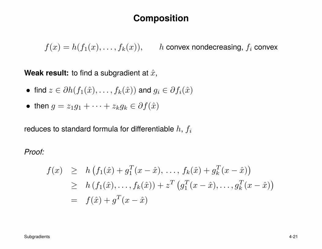
Composition
f(x) = h(f1(x), . . . , fk(x)), h convex nondecreasing, fi convex
Weak result: to find a subgradient at x,
• find z ∈ ∂h(f1(x), . . . , fk(x)) and gi ∈ ∂fi(x)
• then g = z1g1 + · · ·+ zkgk ∈ ∂f(x)
reduces to standard formula for differentiable h, fi
Proof:
f(x) ≥ h(f1(x) + gT1 (x− x), . . . , fk(x) + gTk (x− x)
)≥ h (f1(x), . . . , fk(x)) + zT
(gT1 (x− x), . . . , gTk (x− x)
)= f(x) + gT (x− x)
Subgradients 4-21

Optimal value function
define f(u, v) as the optimal value of convex problem
minimize f0(x)subject to fi(x) ≤ ui, i = 1, . . . ,m
Ax = b+ v
(functions fi are convex; optimization variable is x)
Weak result: suppose f(u, v) is finite and strong duality holds with the dual
maximize infx
(f0(x) +
∑i
λi(fi(x)− ui) + νT (Ax− b− v)
)subject to λ � 0
if λ, ν are optimal dual variables (for r.h.s. u, v) then (−λ,−ν) ∈ ∂f(u, v)
Subgradients 4-22

Proof: by weak duality for problem with r.h.s. u, v
f(u, v) ≥ infx
(f0(x) +
∑i
λi(fi(x)− ui) + νT (Ax− b− v)
)
= infx
(f0(x) +
∑i
λi(fi(x)− ui) + νT (Ax− b− v)
)− λT (u− u)− νT (v − v)
= f(u, v)− λT (u− u)− νT (v − v)
Subgradients 4-23

Expectation
f(x) = Eh(x, u) u random, h convex in x for every u
Weak result: to find a subgradient at x,
• choose a function u 7→ g(u) with g(u) ∈ ∂xh(x, u)
• then, g = Eu g(u) ∈ ∂f(x)
Proof: by convexity of h and definition of g(u),
f(x) = Eh(x, u)
≥ E(h(x, u) + g(u)T (x− x)
)= f(x) + gT (x− x)
Subgradients 4-24
Outline
• definition
• subgradient calculus
• duality and optimality conditions
• directional derivative
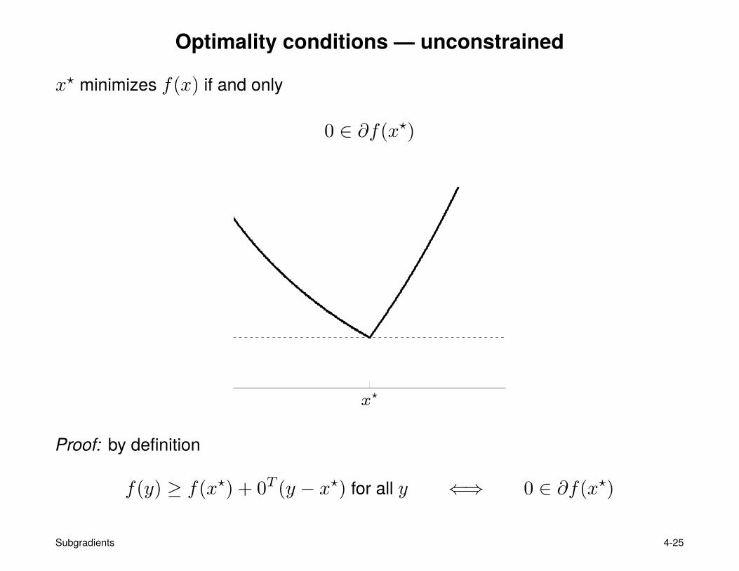
Optimality conditions — unconstrained
x? minimizes f(x) if and only
0 ∈ ∂f(x?)
x?
f(y)
Proof: by definition
f(y) ≥ f(x?) + 0T (y − x?) for all y ⇐⇒ 0 ∈ ∂f(x?)
Subgradients 4-25

Example: piecewise linear minimization
f(x) = maxi=1,...,m
(aTi x+ bi)
Optimality condition
0 ∈ conv {ai | i ∈ I(x?)} where I(x) = {i | aTi x+ bi = f(x)}
• in other words, x? is optimal if and only if there is a λ with
λ � 0, 1Tλ = 1,m∑i=1
λiai = 0, λi = 0 for i 6∈ I(x?)
• these are the optimality conditions for the equivalent linear program
minimize tsubject to Ax+ b � t1
maximize bTλsubject to ATλ = 0
λ � 0, 1Tλ = 1
Subgradients 4-26
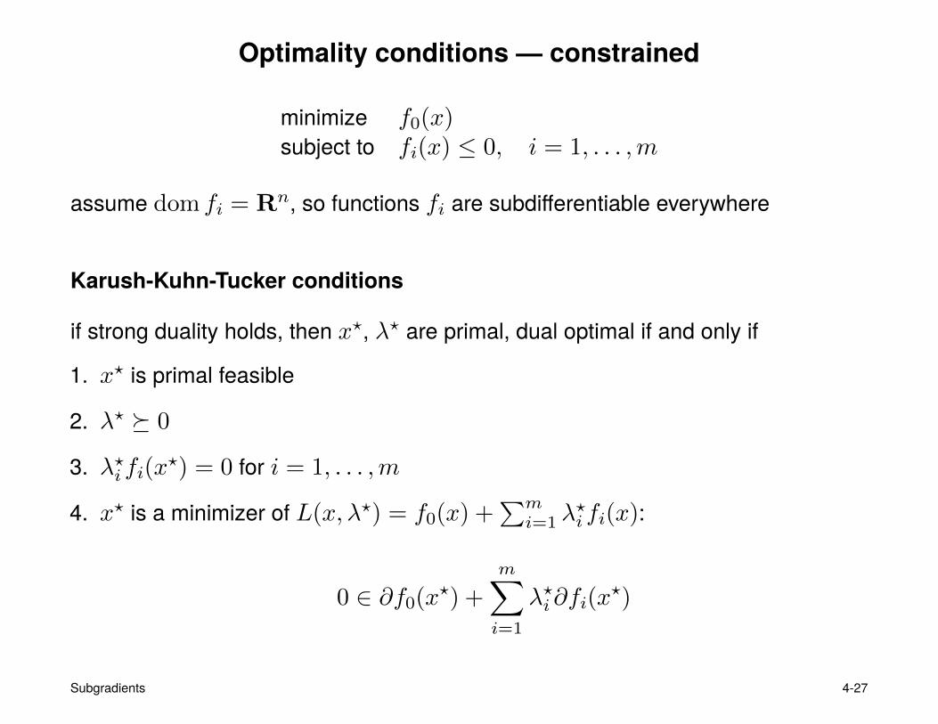
Optimality conditions — constrained
minimize f0(x)subject to fi(x) ≤ 0, i = 1, . . . ,m
assume dom fi = Rn, so functions fi are subdifferentiable everywhere
Karush-Kuhn-Tucker conditions
if strong duality holds, then x?, λ? are primal, dual optimal if and only if
1. x? is primal feasible
2. λ? � 0
3. λ?i fi(x?) = 0 for i = 1, . . . ,m
4. x? is a minimizer of L(x, λ?) = f0(x) +∑mi=1 λ
?i fi(x):
0 ∈ ∂f0(x?) +
m∑i=1
λ?i∂fi(x?)
Subgradients 4-27
Outline
• definition
• subgradient calculus
• duality and optimality conditions
• directional derivative
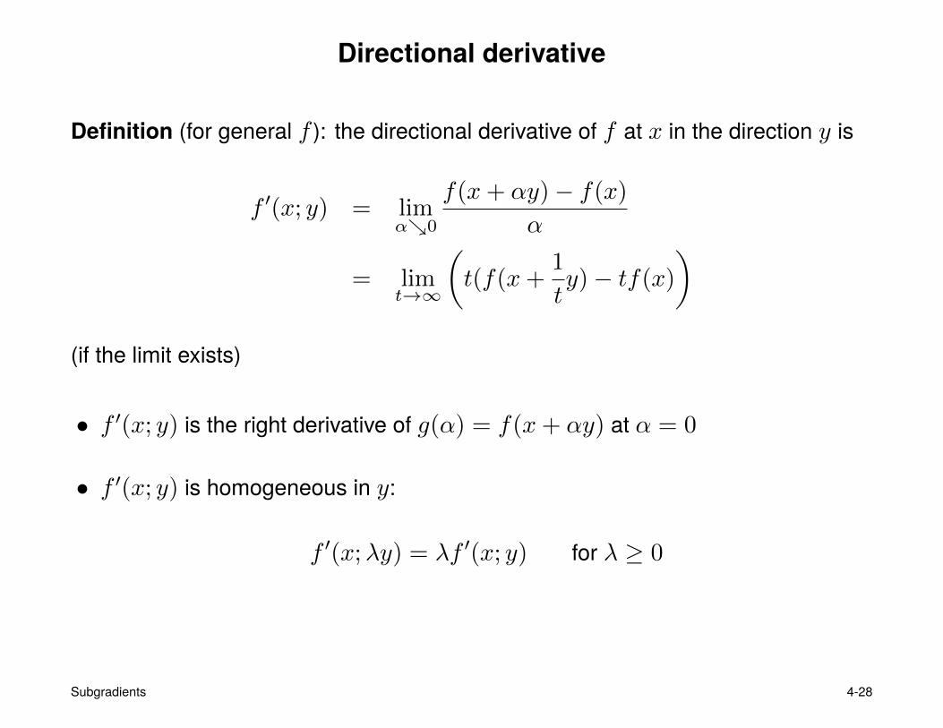
Directional derivative
Definition (for general f ): the directional derivative of f at x in the direction y is
f ′(x; y) = limα↘0
f(x+ αy)− f(x)
α
= limt→∞
(t(f(x+
1
ty)− tf(x)
)(if the limit exists)
• f ′(x; y) is the right derivative of g(α) = f(x+ αy) at α = 0
• f ′(x; y) is homogeneous in y:
f ′(x;λy) = λf ′(x; y) for λ ≥ 0
Subgradients 4-28
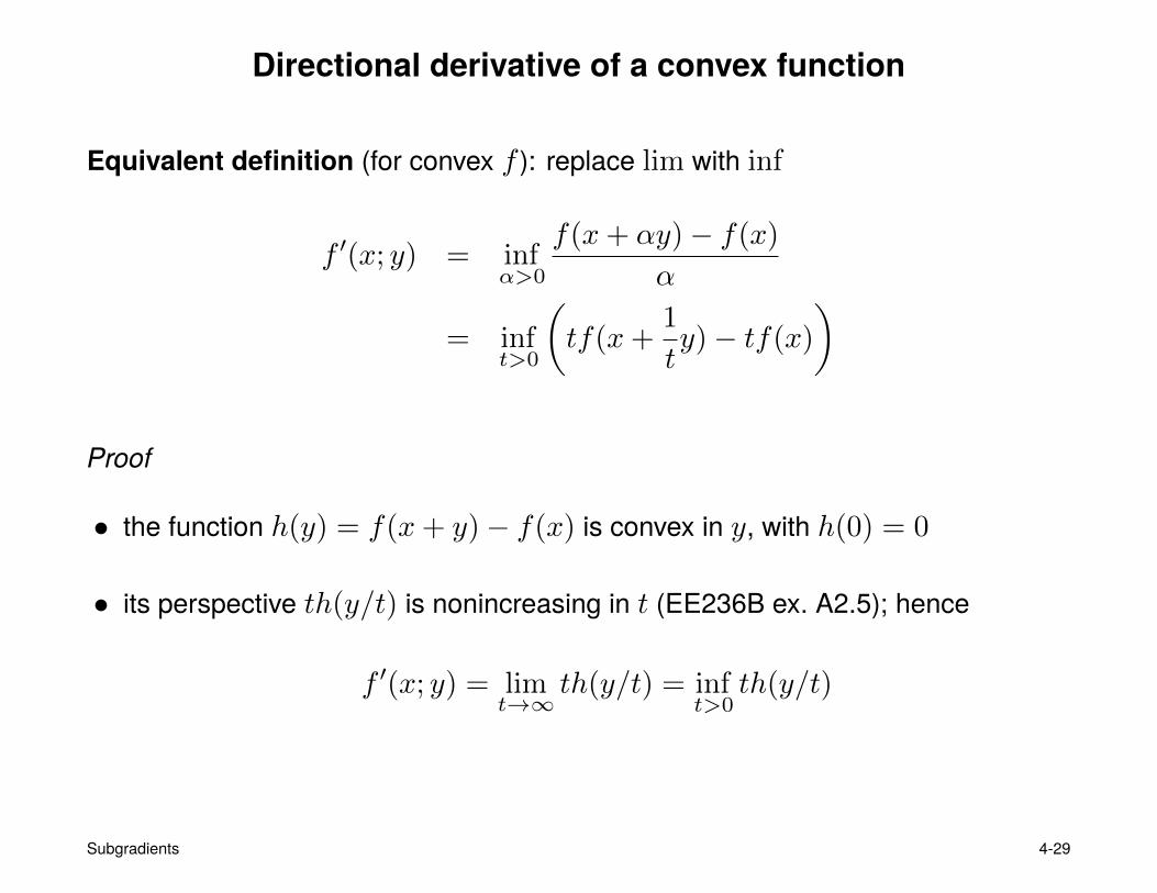
Directional derivative of a convex function
Equivalent definition (for convex f ): replace lim with inf
f ′(x; y) = infα>0
f(x+ αy)− f(x)
α
= inft>0
(tf(x+
1
ty)− tf(x)
)
Proof
• the function h(y) = f(x+ y)− f(x) is convex in y, with h(0) = 0
• its perspective th(y/t) is nonincreasing in t (EE236B ex. A2.5); hence
f ′(x; y) = limt→∞
th(y/t) = inft>0
th(y/t)
Subgradients 4-29

Properties
consequences of the expressions (for convex f )
f ′(x; y) = infα>0
f(x+ αy)− f(x)
α
= inft>0
(tf(x+
1
ty)− tf(x)
)
• f ′(x; y) is convex in y (partial minimization of a convex function in y, t)
• f ′(x; y) defines a lower bound on f in the direction y:
f(x+ αy) ≥ f(x) + αf ′(x; y) ∀α ≥ 0
Subgradients 4-30

Directional derivative and subgradients
for convex f and x ∈ int dom f
f ′(x; y) = supg∈∂f(x)
gTy
g
∂f(x)y
f ′(x, y) = gTy
f ′(x; y) is support function of ∂f(x)
• generalizes f ′(x; y) = ∇f(x)Ty for differentiable functions
• implies that f ′(x; y) exists for all x ∈ int dom f , all y (see page 4-4)
Subgradients 4-31

Proof: if g ∈ ∂f(x) then from p. 4-29
f ′(x; y) ≥ infα>0
f(x) + αgTy − f(x)
α= gTy
it remains to show that f ′(x; y) = gTy for at least one g ∈ ∂f(x)
• f ′(x; y) is convex in y with domain Rn, hence subdifferentiable at all y
• let g be a subgradient of f ′(x; y) at y: for all v, λ ≥ 0,
λf ′(x; v) = f ′(x;λv) ≥ f ′(x; y) + gT (λv − y)
• taking λ→∞ shows f ′(x; v) ≥ gTv; from the lower bound on p. 4-30,
f(x+ v) ≥ f(x) + f ′(x; v) ≥ f(x) + gTv ∀v
hence g ∈ ∂f(x)
• taking λ = 0 we see that f ′(x; y) ≤ gTy
Subgradients 4-32
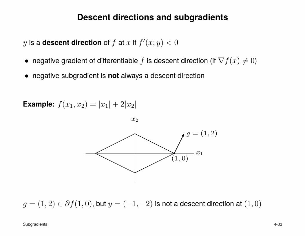
Descent directions and subgradients
y is a descent direction of f at x if f ′(x; y) < 0
• negative gradient of differentiable f is descent direction (if ∇f(x) 6= 0)
• negative subgradient is not always a descent direction
Example: f(x1, x2) = |x1|+ 2|x2|
g = (1, 2)
x1
x2
(1, 0)
g = (1, 2) ∈ ∂f(1, 0), but y = (−1,−2) is not a descent direction at (1, 0)
Subgradients 4-33

Steepest descent direction
Definition: (normalized) steepest descent direction at x ∈ int dom f is
∆xnsd = argmin‖y‖2≤1
f ′(x; y)
∆xnsd is the primal solution y of the pair of dual problems (BV §8.1.3)
minimize (over y) f ′(x; y)subject to ‖y‖2 ≤ 1
maximize (over g) −‖g‖2subject to g ∈ ∂f(x)
• dual optimal g? is subgradient with least norm
• f ′(x; ∆xnsd) = −‖g?‖2
• if 0 6∈ ∂f(x), ∆xnsd = −g?/‖g?‖2
• ∆xnsd can be expensive too compute
∂f(x)
g?
∆xnsdgT∆xnsd = f ′(x,∆xnsd)
Subgradients 4-34
Subgradients and distance to sublevel sets
if f is convex, f(y) < f(x), g ∈ ∂f(x), then for small t > 0,
‖x− tg − y‖22 = ‖x− y‖22 − 2tgT (x− y) + t2‖g‖22≤ ‖x− y‖22 − 2t(f(x)− f(y)) + t2‖g‖22< ‖x− y‖22
• −g is descent direction for ‖x− y‖2, for any y with f(y) < f(x)
• in particular, −g is descent direction for distance to any minimizer of f
Subgradients 4-35
References
• J.-B. Hiriart-Urruty, C. Lemaréchal, Convex Analysis and MinimizationAlgoritms (1993), chapter VI.
• Yu. Nesterov, Introductory Lectures on Convex Optimization. A Basic Course(2004), section 3.1.
• B. T. Polyak, Introduction to Optimization (1987), section 5.1.
Subgradients 4-36


