
LOCAL SEARCH HEURISTICS FOR FACILITY LOCATIONPROBLEMS
VINAYAKA PANDIT
DEPARTMENT OF COMPUTER SCIENCE AND ENGINEERINGINDIAN INSTITUTE OF TECHNOLOGY DELHI
JULY 2004


c© Indian Institute of Technology Delhi (IITD), New Delhi, 2004.

Local Search Heuristics for Facility Location Problems
byVinayaka Pandit
Department of Computer Science and Engineering
Submitted
in fulfillment of the requirements of the degree of
Doctor of Philosophy
to the
Indian Institute of Technology DelhiJuly 2004


Certificate
This is to certify that the thesis titled “Local Search Heuristics for Facility Location Problems”
being submitted by Vinayaka Pandit to the Indian Institute of Technology Delhi, for the award of
the degree of Doctor of Philosophy, is a record of bona-fide research work carried out by him under
my supervision. In my opinion, the thesis has reached the standards fulfilling the requirements of
the regulations relating to the degree.
The results contained in this thesis have not been submitted in part or full to any other university
or institute for the award of any degree/diploma.
Naveen GargAssociate Professor
Department of Computer Science and EngineeringIndian Institute of Technology Delhi
New Delhi 110 016


To my parents and my sisterfor their love and constant support


Acknowledgments
Two people have helped bring this thesis to its fruition. Firstly, Naveen Garg, my advisor. His
penchant for difficult problems, deep results, and highly intuitive understanding of important results
have become guiding principles in my approach to research. His emphasis on easily understandable
presentation has deeply influenced me in presenting my work. No words can express my gratitude
towards him. Secondly, Rohit Khandekar, my colleague for last four years. Rohit got deeply in-
volved in my research and I have thoroughly enjoyed working with him on many different problems.
His clarity of thought is at the top of my wish list. I wish him all the best as he starts his academic
career. I would like to thank Naveen and Rohit profusely for making the last four years, a great
experience in learning.
During my under-graduation, two people helped me discover the joy of research: Raghavendra
Udupa and Dr. Ashok Rao. Ashok brought the first breeze of fresh thought in my undergraduate
college and got many of us interested in research. He guided me in my final year project and our
association continues even today. I would like to thank him for being a great friend, philosopher,
and guide. I worked with Raghavendra Udupa for my final year project. The memory of us working
on weighted finite automata for image compression and eventually succeeding in improving itsdecoding algorithm brings joy even today. We have been colleagues for 12 years now and his
friendship is one of the great treasures of my life. Udu, thank you for everything. When Prof.
Ramasesha taught his first class in my final year, little did I realize that our association would last so
long. His interests are so diverse and insights so deep that, each meeting with him is very special.
These three people have made Mysore, a special place for me.
I recall my days at IIT-Bombay with great pleasure. In those days, the campus used to be a won-
derful place to be in. The Computer Science Department had a vibrant atmosphere, and had a very
enthusiastic student community. Prof. A. A. Diwan taught a wonderful course in Combinatorics
and initiated my interest in Theoretical Computer Science. I thank him for the wonderful course,
and the demanding home assignments.
I would like to thank the management at IBM India Research Lab for supporting me during
these four years. Special thanks to Dr. Alok Aggarwal for his encouragement. I would like to thank
my friends from IRL, Tanveer Faruquie, Sugata Ghosal, Manish Kurhekar, Johara Shahabuddin,
Vijay Kumar, Amit Nanavati, Meeta Sharma, and Krishna Prasad. Their company makes working

in IRL, a pleasant experience. I would also like to acknowledge all my co-authors and thank them
for allowing me to include these results here.
Archana, I am full of hope as we start a new phase in our life. I thank you for your love, care,
and understanding. At the end, I have to mention three people to whom I dedicate this thesis. It is
impossible to recall all that they have given me. I hope I have been worthy of it. My father, my
mother, and my sister. Thank you for everything.
July 2004 Vinayaka Pandit

Abstract
In this thesis, we develop approximation algorithms for facility location problems based on local
search techniques. Facility location is an important problem in operations research. Heuristic ap-
proaches have been used to solve many variants of the problem since the 1960s. The study of
approximation algorithms for facility location problems started with the work of Hochbaum. Al-
though local search is a popular heuristic among practitioners, their analysis from the point of view
of approximation started only recently. In a short time, local search has emerged as a versatile tech-
nique for obtaining approximation algorithms for facility location problems. Significantly, there are
many variants for which local search is the only technique known to give constant factor approx-imations. In this thesis, we demonstrate the effectiveness of local search for facility location by
obtaining approximation algorithms for many diverse variants of the problem.
Local search is an iterative heuristic used to solve many optimization problems. Typically, a
local search heuristic starts with any feasible solution, and improves the quality of the solution
iteratively. At each step, it considers only local operations to improve the cost of the solution. A
solution is called a local minima if there is no local operations which improves the cost. One of
the earliest and most popular local search heuristic for facility location was proposed by Kuehn and
Hamburger in the 1960s. However, the analysis of a local minima for the worst case ratio of its
cost to the cost of the optimal solution began only recently with the work of Korupolu, Plaxton, and
Rajaraman. Since then, their analysis has been improved, and local search heuristics for diverse
variants of facility location have been presented. Informally, locality gap is the worst case ratio of
the cost of a local minima to the cost of the global optima.
We present the first analysis of a local search algorithm which gives a constant factor approxi-
mation for the k-median problem while opening at most k facilities. Our analysis yields a 3(1 + ε)
approximation algorithm for the k-median problems which is the best known ratio currently. We
show that our technique can be used to analyze local search algorithms for the uncapacitated facility
location problem, capacitated facility location problem with soft capacities, k-uncapacitated facility
location problem, and a bi-criteria facility location problem. Our analysis yields 3(1 + ε) approxi-
mation algorithm for the uncapacitated facility location, 4(1 + ε) approximation for the capacitated
facility location with soft capacities, and 5(1 + ε) approximation for the k-uncapacitated facility
location problem. We establish an interesting connection between the price of anarchy of a service
provider game and the locality gap of k-uncapacitated facility location problem. This gives rise to
the possibility of reducing the question of upper bounding the price of anarchy of certain games to

the question of upper bounding the locality gap of their corresponding optimization problems.

Contents
List of Figures xv
1 Introduction 1
2 Overview 52.1 Facility Location Problems . . . . . . . . . . . . . . . . . . . . . . . . . . . . . . 5
2.1.1 k-median problem . . . . . . . . . . . . . . . . . . . . . . . . . . . . . . 6
2.1.2 Uncapacitated Facility Location (UFL) . . . . . . . . . . . . . . . . . . . 6
2.1.3 k-Uncapacitated Facility Location (k-UFL) . . . . . . . . . . . . . . . . . 6
2.1.4 Facility Location with Soft Capacities (∞-CFL) . . . . . . . . . . . . . . 7
2.1.5 Universal Facility Location Problem (UniFL) . . . . . . . . . . . . . . . . 7
2.1.6 Budget Constrained k-median problem . . . . . . . . . . . . . . . . . . . 8
2.2 Techniques for Facility Location . . . . . . . . . . . . . . . . . . . . . . . . . . . 9
2.2.1 Greedy Heuristics . . . . . . . . . . . . . . . . . . . . . . . . . . . . . . . 9
2.2.2 LP Rounding Techniques . . . . . . . . . . . . . . . . . . . . . . . . . . . 9
2.2.3 Primal-Dual Techniques . . . . . . . . . . . . . . . . . . . . . . . . . . . 10
2.2.4 Local Search Techniques . . . . . . . . . . . . . . . . . . . . . . . . . . . 10
2.3 Local Search Technique . . . . . . . . . . . . . . . . . . . . . . . . . . . . . . . . 10
2.3.1 Local Search and Locality Gap . . . . . . . . . . . . . . . . . . . . . . . . 11
2.3.2 Analysis Technique . . . . . . . . . . . . . . . . . . . . . . . . . . . . . . 122.4 Local Search and Approximation Classes . . . . . . . . . . . . . . . . . . . . . . 14
2.4.1 Guaranteed Local Optima(GLO) . . . . . . . . . . . . . . . . . . . . . . . 14
2.4.2 MAX SNP and Non-oblivious Local Search . . . . . . . . . . . . . . . . . 14
2.4.3 Local Search and Approximation . . . . . . . . . . . . . . . . . . . . . . 15
xi

3 The k-median problem 173.1 Preliminaries . . . . . . . . . . . . . . . . . . . . . . . . . . . . . . . . . . . . . 17
3.2 Notations . . . . . . . . . . . . . . . . . . . . . . . . . . . . . . . . . . . . . . . 19
3.3 Local search with single swaps . . . . . . . . . . . . . . . . . . . . . . . . . . . . 20
3.3.1 The analysis . . . . . . . . . . . . . . . . . . . . . . . . . . . . . . . . . 20
3.3.2 Local search with multi-swaps . . . . . . . . . . . . . . . . . . . . . . . . 26
3.3.3 Analysis . . . . . . . . . . . . . . . . . . . . . . . . . . . . . . . . . . . 27
3.3.4 Tight example . . . . . . . . . . . . . . . . . . . . . . . . . . . . . . . . 29
4 The uncapacitated facility location problem 314.1 Uncapacitated Facility Location Problem . . . . . . . . . . . . . . . . . . . . . . 31
4.1.1 Preliminaries . . . . . . . . . . . . . . . . . . . . . . . . . . . . . . . . . 31
4.1.2 A local search procedure . . . . . . . . . . . . . . . . . . . . . . . . . . . 32
4.1.3 The analysis . . . . . . . . . . . . . . . . . . . . . . . . . . . . . . . . . 33
4.1.4 Tight example . . . . . . . . . . . . . . . . . . . . . . . . . . . . . . . . 37
4.2 The Capacitated Facility Location Problem . . . . . . . . . . . . . . . . . . . . . 38
4.2.1 A local search algorithm . . . . . . . . . . . . . . . . . . . . . . . . . . . 394.2.2 The analysis . . . . . . . . . . . . . . . . . . . . . . . . . . . . . . . . . 40
5 The k-uncapacitated facility location problem 435.1 Motivation . . . . . . . . . . . . . . . . . . . . . . . . . . . . . . . . . . . . . . . 43
5.2 Preliminaries . . . . . . . . . . . . . . . . . . . . . . . . . . . . . . . . . . . . . 46
5.2.1 Service provider game . . . . . . . . . . . . . . . . . . . . . . . . . . . . 46
5.2.2 The k-UFL problem . . . . . . . . . . . . . . . . . . . . . . . . . . . . . 46
5.3 Price of Anarchy and Locality Gap . . . . . . . . . . . . . . . . . . . . . . . . . . 47
5.4 Locality Gap of the k-UFL Problem . . . . . . . . . . . . . . . . . . . . . . . . . 49
5.4.1 Notations . . . . . . . . . . . . . . . . . . . . . . . . . . . . . . . . . . . 49
5.4.2 Deletes and Swaps considered . . . . . . . . . . . . . . . . . . . . . . . . 50
5.4.3 Bounding the increase in the facility cost . . . . . . . . . . . . . . . . . . 51
5.4.4 Bounding the increase in the service cost . . . . . . . . . . . . . . . . . . 52
5.4.5 Bounding the increase in the total cost . . . . . . . . . . . . . . . . . . . . 55

6 The universal facility location problem 576.1 Preliminaries . . . . . . . . . . . . . . . . . . . . . . . . . . . . . . . . . . . . . 57
6.2 Local Search Heuristic . . . . . . . . . . . . . . . . . . . . . . . . . . . . . . . . 59
6.3 Implementation . . . . . . . . . . . . . . . . . . . . . . . . . . . . . . . . . . . . 60
6.4 Locality Gap . . . . . . . . . . . . . . . . . . . . . . . . . . . . . . . . . . . . . 61
6.4.1 A transshipment problem . . . . . . . . . . . . . . . . . . . . . . . . . . . 62
6.4.2 Structure of Minimum Transshipment . . . . . . . . . . . . . . . . . . . . 63
6.4.3 Analysis . . . . . . . . . . . . . . . . . . . . . . . . . . . . . . . . . . . 64
7 The budget constrained k-median problem 697.1 Motivation . . . . . . . . . . . . . . . . . . . . . . . . . . . . . . . . . . . . . . . 69
7.2 A simple scheme that fails . . . . . . . . . . . . . . . . . . . . . . . . . . . . . . 72
7.3 Computing a Bounded Diameter Partition . . . . . . . . . . . . . . . . . . . . . . 73
7.3.1 Triplet Phase . . . . . . . . . . . . . . . . . . . . . . . . . . . . . . . . . 74
7.3.2 Doublet Phase . . . . . . . . . . . . . . . . . . . . . . . . . . . . . . . . 75
7.3.3 Singlet Phase . . . . . . . . . . . . . . . . . . . . . . . . . . . . . . . . . 76
7.3.4 Generalization . . . . . . . . . . . . . . . . . . . . . . . . . . . . . . . . 777.4 Restricted Local Search . . . . . . . . . . . . . . . . . . . . . . . . . . . . . . . . 78
7.5 Analysis of Locality Gap . . . . . . . . . . . . . . . . . . . . . . . . . . . . . . . 79
8 Conclusions and open problems 83
Bibliography 85


List of Figures
2.1 A generic local search algorithm . . . . . . . . . . . . . . . . . . . . . . . . . . . 12
3.1 Notions of neighborhood of a facility and service cost of a client . . . . . . . . . . 20
3.2 Local Search heuristic for the k-median problem . . . . . . . . . . . . . . . . . . 20
3.3 Partitioning the neighborhood of a facility o ∈ O . . . . . . . . . . . . . . . . . . 21
3.4 The mapping π on NO(o) . . . . . . . . . . . . . . . . . . . . . . . . . . . . . . . 23
3.5 Capture Graph H = (S,O,E) . . . . . . . . . . . . . . . . . . . . . . . . . . . . 24
3.6 k swaps considered in the analysis . . . . . . . . . . . . . . . . . . . . . . . . . . 24
3.7 Reassigning the clients in NS(s) ∪NO(o). . . . . . . . . . . . . . . . . . . . . . . 25
3.8 A procedure to define the partitions . . . . . . . . . . . . . . . . . . . . . . . . . . 27
3.9 Tight example for 2-swap heuristic . . . . . . . . . . . . . . . . . . . . . . . . . . 29
4.1 Reassigning a client j ∈ NS(s) when a good facility s is dropped. . . . . . . . . . 34
4.2 Bounding the facility cost of a bad facility s: (a) Reassignment when π(j) 6∈ NS(s)
(b) Reassignment when π(j) ∈ NS(s) and j 6∈ NO(o) (c) Reassignment of j ∈NO(o′) when o′ ∈ P − {o} is added. . . . . . . . . . . . . . . . . . . . . . . . . . 35
4.3 Tight example for the locality gap of UFL. . . . . . . . . . . . . . . . . . . . . . . 37
4.4 A procedure to find a subset T ⊆ S of facilities . . . . . . . . . . . . . . . . . . . 40
4.5 The flow graph . . . . . . . . . . . . . . . . . . . . . . . . . . . . . . . . . . . . 41
5.1 Rerouting a client j ∈ NO(o) when o is brought in . . . . . . . . . . . . . . . . . 52
5.2 Rerouting a client j ∈ NS(s) when s is taken out, and the facility serving it in
the optimal solution is not brought in: Right hand side shows the rerouting when
π(j) 6∈ NS(s). Left hand side shows the rerouting when π(j) = j and s is a 2+bad
facility. We swap s with o, its near facility. Here, j ∈ NO(o′) and s captures o′. . . 53
xv

6.1 The subtree T t . . . . . . . . . . . . . . . . . . . . . . . . . . . . . . . . . . . . 64
6.2 Reassigning the demand for the Single Pivot, and Double Pivot operations. . . . . 65
7.1 Example where approximating 2-median and 2-center within constant factors is not
possible. . . . . . . . . . . . . . . . . . . . . . . . . . . . . . . . . . . . . . . . . 70
7.2 Sometimes medians can be fair to all clients. . . . . . . . . . . . . . . . . . . . . . 70
7.3 Illustration of a triplet region . . . . . . . . . . . . . . . . . . . . . . . . . . . . . 74
7.4 Illustration of a doublet region . . . . . . . . . . . . . . . . . . . . . . . . . . . . 75
7.5 Illustration of a singlet region . . . . . . . . . . . . . . . . . . . . . . . . . . . . . 76
7.6 Restricted Local Search . . . . . . . . . . . . . . . . . . . . . . . . . . . . . . . . 79
7.7 Reassigning the clients in NS(s) ∪NO(o). . . . . . . . . . . . . . . . . . . . . . . 81

Chapter 1
Introduction
Optimizing the cost of repetitive tasks is an important exercise in operations research. Organizations
of even modest sizes optimize their operations to minimize costs and improve efficiency. One
of the many aspects of operations is cost effective and efficient accessing of a set of services or
infrastructural facilities by a group of demand points or clients. Typically, many service locations are
set up, each of which serves the demands of a subset of demand points. Some examples of such an
exercise are setting up of a supply chain of a business, locating essential services such as health care
and education, and construction of transportation networks. Facility location problems proposed
in operations research provide mathematical formulations of the common optimization aspects of
these problems. We begin by describing example scenarios where facility location formulations are
natural.
Consider an automobile service company which aims to provide its customer with efficient
access to service stations. To do so, it would like to ensure that, all its customers have a nearby
service station. However, the company incurs significant cost in setting up each service station. So,
opening a large number of service station may be prohibitively costly. Ideally, the company would
like to open a fixed number of service stations such that the average distance of its customers to
their nearest service station is minimum.
Consider the problem of organizing training camps for a large group of people. Most of the
costs involved including setting up of the camps, and the logistics of transport for the people are
incurred just once. In such a scenario, one would like to open a set of training facilities and assign
people to the training facilities such that the cost of the entire exercise, i.e, the cost of setting up thefacilities and the cost of transporting people to the facilities is minimized.
1

2 CHAPTER 1. INTRODUCTION
The facility location problems capture the common features of the problems described above.
The goal of facility location is to serve a set of demand points, typically called as clients, by a
opening a set of access points, typically called as facilities, in a cost effective and efficient manner.
The distances between the clients and facilities are assumed to satisfy metric properties. There is
a location dependent cost for opening a facility at each location. Typically, a solution to a facility
location problem is specified by a set of facilities to be opened and an assignment of the clients to
the open facilities. The sum of costs of opening the facilities is called the facility cost, and the sum
of distances of each client to the facility it is assigned to is called as the service cost of the solution.
Different variants of the facility location problem are obtained by combining these costs in different
ways. A richer set of problems emerges by considering formulations in which each facility can
serve at most a specified number of clients or by making the cost of a facility depend on the number
of clients it serves after the assignment. A comprehensive treatment of facility location problems
and their formulations can be found in [15, 40, 45].
It is clear that facility location is a very important aspect of organizational tasks. Naturally,
they have been solved for a long time now. The advent of computers fostered interest in obtaining
efficient and optimal solutions to these problems. But, most variants of facility location are NP-
Complete. So, efficient algorithms which compute solutions which are close to the optimal solution
are desirable. In the last few years, approximation algorithms for facility location problems havegained attention of many researchers.
In the past few years, many approaches have been proposed to develop approximation algo-
rithms for facility location problems. Greedy heuristics were the first to be proposed and have been
refined ever since. Another popular approach is to consider the linear program relaxation of the
integer program formulation, and round an optimal fractional solution so as to guarantee good ap-
proximations. Primal-dual algorithms based on the integer program formulations have also been
used successfully. Combination of greedy heuristics with primal-dual techniques have obtained
very good results for certain varieties of facility location problems. However, techniques based on
local search have been used successfully for approximating the largest variety of facility locations
problems. For certain variations of the facility location problems, local search gives the best known
approximation factor of all the proposed approaches and for certain other variations, local search is
the only technique known to give acceptable bounds.
In this thesis, we present local search heuristics for a wide range of facility location problems
and analyze their approximation guarantees. We also establish an interesting connection between
the price of anarchy of a network service provider game and the locality gap of the corresponding

3
facility location problem. This gives rise to the possibility of reducing the question of upper bound-
ing of the price of anarchy of certain games to the question of upper bounding the locality gap of
the corresponding optimization problems.

4 CHAPTER 1. INTRODUCTION

Chapter 2
Overview
In this chapter, we present an overview of this thesis. In Section 2.1, we define the problems consid-
ered in this thesis. In Section 2.2, we present a brief summary of the known techniques for facility
location. In Section 2.3, we present an overview of the local search technique for combinatorial
optimization problems.
2.1 Facility Location Problems
As described in chapter 1, the set of facility locations or simply, facilities, and the set of clients
form a part of the input for all facility location variants. We denote the set of facilities by F and
the set of clients by C . Typically, we are required to open a subset of the facilities and serve the
demands of clients by assigning them to one of the open facilities. The distance between a pair ofpoints i, j ∈ F ∪ C is denoted by cij . The distances are symmetric, satisfy triangle inequalities,
and cij = 0, if and only if i = j. Thus, the distances define a metric. Suppose S is a set of open
facilities, then ∀i ∈ C , dist(i, S) denotes the minimum distance between i and a facility in S. If a
client j is served by a facility i in a solution, then the distance cij is said to be the service cost of
client j. The sum of service costs of all clients is the service cost of the solution. Depending on the
variant we are dealing with, there is a cost associated with opening a facility at i ∈ F , denoted by
fi. For a given solution, the cost of opening all the open facilities is called its facility cost. Certain
variants of facility location may also place a limit on the number of clients a facility can serve,
namely its capacity.
A rich set of facility location problems emerges by mixing the facility costs, service costs, and
5
6 CHAPTER 2. OVERVIEW
the capacity constraints differently. As demonstrated in this thesis, local search provides a unified
approach to obtain approximation algorithms for these problems.
2.1.1 k-median problem
This problem is motivated by scenarios in which a limited budget is available for opening the facil-
ities and the cost of all the facilities are roughly the same.
• Input: The set of facilities F , the set of clients C , and the distance metric. Input also consists
of an integer k which is the maximum number of facilities that can be opened.
• Output: Find a set S ⊆ F such that |S| ≤ k, and∑
i∈C dist(i, S) is minimized.
We show that a simple local search heuristic gives a 3(1 + ε) approximation for the k-median
problem. Currently, this is the best known approximation ratio for the k-median problem.
2.1.2 Uncapacitated Facility Location (UFL)
There are facility location situations in which both the facility cost and service cost are incurred
only once. The UFL problem models such scenarios.
• Input: The set of facilities F , the set of clients C , and the distance metric. For each i ∈ F ,
the cost of opening a facility at i, denoted by fi, is also given.
• Output: Find a set S ⊆ F such that (∑
i∈S fi +∑
i∈C dist(i, S)) is minimized.
We provide a local search heuristic with a 3(1 + ε) approximation for the UFL problem. Our
algorithm considers very simple local operations.
2.1.3 k-Uncapacitated Facility Location (k-UFL)
This problem is a variant of uncapacitated facility location in which a limit is placed on the number
of facilities which can be opened.
• Input: The set of facilities F , the set of clients C , an integer k, and the distance metric. For
each i ∈ F , cost of opening a facility at i, denoted by fi, is also given.
• Output: Find a set S ⊆ F such that |S| ≤ k and (∑
i∈S fi +∑
i∈C dist(i, S)) is minimized.

2.1. FACILITY LOCATION PROBLEMS 7
Note that, k-UFL is a generalization of 2.1.1 and 2.1.2. It reduces to the k-median problem if all
the facility costs are zero and reduces to the UFL if k is equal to the number of the facilities in
F . We [16] give the first known analysis of a local search heuristic for this problem and obtain an
approximation factor of 5(1 + ε). We also establish an interesting connection between the local
optimum of this problem and the worst-case equilibria of a related network service provider game.
2.1.4 Facility Location with Soft Capacities (∞-CFL)
The uncapacitated facility location ignores the fact that the cost of a facility could depend on the
number of clients it serves. This problem attempts to take this aspect into account by associating
capacities with the facilities and making the cost of facility vary linearly with respect to the numberof clients it serves modulo its original capacity.
• Input: The set of facilities F , the set of clients C , and the distance metric. For each i ∈ F ,
cost of opening a facility at i denoted by fi, and a capacity ui which is the maximum number
of clients a facility at i can serve.
• Output: A function h from the set of facilities to the set of integers, h : F → N, the set
of natural numbers. It specifies the number of copies of a facility being opened. Output also
consists of an assignment of clients to the set of facilities, g : C → F . The assignment shouldbe such that (si = |{j ∈ C|g(j) = i}| ≤ h(i) · ui),∀i ∈ F . In other words, we have to open
a subset of facilities (multiple copies of a facility can be allowed which increases its capacity
by a factor of its original capacity) and assign clients to the open facilities such that no facility
serves more than its effective capacity. The goal is to minimize∑
i∈F h(i) ·fi +∑
j∈C cjg(j),
i.e, minimize the total cost of opening the facilities and service cost of all clients.
Note that the capacities at the facilities are not uniform. We present the first local search algorithm
for∞-CFL with non-uniform capacities. We show that our algorithm has an approximation ratio of
4(1 + ε).
2.1.5 Universal Facility Location Problem (UniFL)
In the ∞-CFL problem, the cost of a facility scales linearly with the number of clients it serves
module its capacity. A generalization of this feature would be to allow the cost of a facility to be
a function of the number of clients it serves. The UniFL problem generalizes the ∞-CFL in this
manner.

8 CHAPTER 2. OVERVIEW
• Input.The set of facilities F , the set of clients C , and the distance metric between them. For
each i ∈ F we are given a function Gi(.) which is assumed to be non-decreasing, and left-
continuous mapping from non-negative reals to non-negative reals. Gi represents the cost of
the facility i depending on the number of clients it serves, i.e, its load.
• Output. Let S ⊆ F be the set of facilities opened and let M be a mapping from clients to S,
i.e, M : C → S. Thus, for j ∈ C , M(j) denotes the facility in S to which j is assigned. For
each i ∈ S, ni denotes the number of clients that i serves , i.e, ni = |{j ∈ C|M(j) = i}|.The goal is to identify a set S and an assignment M of clients to the facilities in S in such
that∑
i∈S Gi(ni) +∑
j∈C cM(j)j is minimized.
In the above formulation, all the clients are assumed to have unit demand. The function Gi is defined
to capture when the demands can be arbitrary and demand of a client can be split across facilities.
Consider a special case of∞-CFL in which a single copy of a facility is allowed to be opened. This
can be specified by an UniFL instance in which Gi(x) = fi if x ≤ ui and ∞, otherwise. This
version of facility location is called Capacitated Facility Location with Hard Capacities or 1-CFL.
2.1.6 Budget Constrained k-median problem
We introduce the following problem motivated by the contrasting objectives of the k-median and
k-center problems. The objective function in k-median problem minimizes the average distance
traveled by the clients. In the k-center problem, the goal is to open k facilities such that the maxi-
mum distance of any client from its nearest facility is minimized. In many situations, it is desirable
to obtain a simultaneous approximation for both the problems. We consider the problem of min-
imizing the total service cost of when a limit is placed on the maximum service cost that can be
incurred by a client.
• Input: The set of clients C . The distances between clients in C satisfy metric properties.
Input also consists of an integer k and a budget B. For a client j ∈ C and a set S ⊆ C ,
ds(j, S) denotes mini∈S
cij .
• Validity: A valid solution S ⊆ C is such that, (|S| ≤ k) ∧ (∀ i ∈ C : ds(i, S) ≤ B).
• Assumption: The input has at least one valid solution.
• Output: A valid solution S such that∑
i∈C ds(i, S) is minimized.

2.2. TECHNIQUES FOR FACILITY LOCATION 9
The nature of the k-median problem and the k-center problem makes it impossible to obtain a
solution which is good with respect to both these measures. So, we relax the constraints by allowing
the budget on the k-center measure to be exceeded by a constant factor. We say that an algorithm
gives (α, β) approximation for this problem if it opens k facilities whose median cost is at most α
times the cost of the optimal valid solution while its induced center cost is at most βB. We give a
local search algorithm for this problem with a pre-processing stage.
2.2 Techniques for Facility Location
The study of approximation algorithms for facility location began with the work of Hochbaum [23].
Research in the last decade has improved the state of the art dramatically. We give an overview of
the different techniques which have been used successfully to approximate some variants of facility
location.
2.2.1 Greedy Heuristics
Approximation algorithms based on greedy heuristics were the first to be proposed for facility loca-
tion problems by Hochbaum [23]. She reduced the facility location problems to variants of set cover
and proposed algorithms along the lines of the greedy heuristic for the set cover problem, and proved
O(log n) bounds. Recently, Jain et al. [25] showed that the same algorithm can be shown to provideconstant factor approximation for uncapacitated facility location. A modified greedy algorithm for
uncapacitated facility location problem was analyzed by Jain et al. [26] using factor revealing LP
which exploits the special properties of the heuristic and also the structure of the problem.
2.2.2 LP Rounding Techniques
Approximation algorithms based on rounding the fractional optimal solution to the LP relaxation
of the original integer programs were proposed by Shmoys et al. [53]. They used the filtering idea
proposed by Lin and Vitter [38] to round the fractional solution to the LP and obtain constant factor
approximations for many facility location problems. This idea was also combined with randomiza-
tion by Chudak and Shmoys [13].

10 CHAPTER 2. OVERVIEW
2.2.3 Primal-Dual Techniques
Approximation algorithms for facility location based on primal-dual techniques were proposed byJain and Vazirani [27]. They solved the uncapacitated facility location problem using a two-phase
primal-dual scheme. Their technique’s novelty was in relaxing the primal conditions while satis-
fying all the complimentary slackness conditions. This allowed them to prove a stronger approxi-
mation theorem for uncapacitated facility location. This also allowed them to obtain approximation
algorithms for a variety of facility location problems including the k-median problem using the
Lagrangian relaxation technique.
2.2.4 Local Search Techniques
Approximation algorithms for facility location based on local search are perhaps the most versatile.
Local search heuristics have been used for many years by practitioners and one such heuristic wasproposed by Kuehn and Hamburger [35]. However, Korupolu et al. [32] showed for the first time
that a worst case analysis of the local minimas computed by these heuristics was possible and they
showed constant factor approximations to many facility location problems which were comparable
to those obtained by other techniques. The significance of these results lies in the fact that local
search is routinely implemented by most practitioners of operations research. For certain variants
of facility location problems, local search is the only technique known to give constant factor ap-
proximations.
2.3 Local Search Technique
In this section, we discuss the local search technique for combinatorial optimization problems.
Local search algorithms have been popular among practitioners due to their ease of understanding
and implementation. For many optimization problems, local search heuristics are also method of
choice for implementation. We begin by briefly surveying the use of local search heuristics in
designing algorithms for combinatorial optimization problems.
Local search techniques have been very popular as heuristics for hard combinatorial optimiza-tion problems. The 1-exchange heuristic by Lin and Kernighan [39] for the metric-TSP remains
the method of choice for practitioners. However, most of these heuristics have poor worst-case
guarantees and very few approximation algorithms that rely on local search are known. Furer and
Raghavachari [17] proposed the first non-trivial approximation algorithm based on local search.

2.3. LOCAL SEARCH TECHNIQUE 11
They considered local search for the problem of computing spanning trees whose maximum degree
is minimum. Their algorithm computed a spanning tree and Steiner trees within an additive loga-
rithmic error of the optimum. It computes a spanning tree whose degree is at most O(∆∗ + log n)
where ∆∗ is the degree of some optimal tree and n is the number of nodes in the input graph. Subse-
quently, local search was used to design approximation algorithms for degree constrained network
design problems. Ravi, Raghavachari, and Klein [49] generalized the above approach to design lo-
cal search heuristics for the problem of finding one-connected networks that are cut-covers of proper
functions such that the maximum degree of any node in the network is minimum. They gave quasi-
polynomial (nO(log1+ε n)-time) algorithm which computes solutions whose maximum degree is at
most (1 + ε) times the minimum with an additive error of O(log1+ε n), for any ε > 0. Lu and Ravi
[41] consider local search for the problem of computing the spanning tree with maximum number of
leaf nodes. They prove approximation guarantees of 5 and 3 for 1-change and 2-change local search
heuristics respectively. Two spanning trees T1 and T2 of an n-node graph are said to be distance k
apart if they have (n− 1− k) edges in common. A k-change heuristic for the above problem con-
siders trees which are at most distance k from the current solution for local improvement. Khanna
et al. [29] showed that a simple local search algorithm for a special case of TSP in which all the
edge lengths are restricted to be 1 or 2, gives an approximation of 3/2. They also showed that their
analysis is tight. Konemann and Ravi [31] used local search algorithms for degree-bounded mini-mum spanning trees. Chandra et al. [7] show an approximation factor of 4
√n for the 2-exchange
local search heuristic for the Euclidean traveling salesman problem. Khuller et al. [30] give a local
search approximation algorithm for finding a feedback edge-set incident upon the minimum number
of vertices. Local search has also been used for set packing problems by Arkin and Hassin [2]. The
study of local search heuristics for facility location problems began with the work of Korupolu et
al. [32] who first showed that the heuristics proposed by Kuehn and Hamburger [35] yield bounds
which are comparable to those obtained by other methods.
2.3.1 Local Search and Locality Gap
A generic local search algorithm is shown in Figure 2.1. Consider an optimization problem P and
an instance I of the problem. A local search algorithm LS(P ) produces a solution to the instance
I by iteratively exploring the space of all feasible solutions to I . Formally, the algorithm can be
described by the set S of all feasible solutions to the input instance, a cost function cost : S → IR, a
neighborhood structureN : S → 2S and an oracle that given any solution S ∈ S , finds (if possible)

12 CHAPTER 2. OVERVIEW
a solution S ′ ∈ N (S) such that cost(S ′) < cost(S). A solution S ∈ S is called local optimum
if cost(S) ≤ cost(S ′) for all S ′ ∈ N (S). The algorithm in Figure 2.1 returns a locally optimum
solution. The cost function and the neighborhood structure N will vary depending on the problem
and the heuristic being employed. The neighborhood structure usually specifies the local operations
allowed at each step. In case of facility location problems, the algorithm described in Figure 2.1 can
be modified suitably to run it in polynomial time and argue approximability. Our description of a
local search algorithm is similar to the description given by Yannakakis [57].
Algorithm Local Search.
1. S ← an arbitrary feasible solution in S .2. While ∃S ′ ∈ N (S) such that cost(S ′) < cost(S),
do S ← S′.3. return S.
Figure 2.1: A generic local search algorithm
Consider a minimization problem P and a local search procedure to solve P , denoted by LS(P ).
For an instance I of the problem P , let global(I) denote the cost of the global optimum and
local(I) be the cost of a locally optimum solution provided by LS(P ). We call the supremum of
the ratio local(I)/global(I), the locality gap of LS(P ).
2.3.2 Analysis Technique
In this section, we present a general framework for running local search heuristics efficiently and to
convert the argument for locality gap into an approximation algorithm for the problem.
The generic algorithm shown in Figure 2.1 may not always terminate in polynomial time. To
run it polynomial time, we modify step 2 of the algorithm as follows.
2M. While ∃S ′ ∈ N (S) such that cost(S ′) ≤ (1− ε/Q) cost(S),
do S ← S′.
Here ε > 0 is a constant and Q is a suitable integer which is polynomial in the size of the input.
Thus, in each local step, the cost of the current solution decreases by a factor of at least ε/Q. If
O denotes an optimum solution and S0 denotes the initial solution, then the number of steps in the
algorithm is at most log(cost(S0)/cost(O))/ log 11−ε/Q . As Q, log(cost(S0)), and log(cost(O))

2.3. LOCAL SEARCH TECHNIQUE 13
are polynomial in the input size, the algorithm terminates after polynomially many local search
steps. We choose Q such that, the algorithm with the above modification continues to have a small
locality gap.
We now present a generic technique for proving a bound on the locality gap. If S is a locally
optimum solution then for all S ′ ∈ N (S),
cost(S′)− cost(S) ≥ 0.
The key to arguing locality gap is to identify a suitable, polynomially large(in the input size)subset Q ∈ N (S) of neighboring solutions which satisfies the following property:
∑
S′∈Q
(cost(S′)− cost(S)) ≤ α · cost(O)− cost(S)
where O is an optimum solution and α > 1 is a suitable constant. But,∑
S′∈Q(cost(S′)− cost(S)) ≥ 0 as S is locally optimum. This implies that cost(S) ≤ α · cost(O)
and gives a bound of α on the locality gap.
Let us now consider a solution S output by the algorithm after incorporating the modified step
2M (with Q = |Q|). To analyze the quality of S, we note that for all S ′ ∈ Q, cost(S ′) > (1 −ε/Q)cost(S). Hence
α · cost(O)− cost(S) ≥∑
S′∈Q
(cost(S′)− cost(S)) > −ε · cost(S)
which implies that cost(S) ≤ α(1−ε)cost(O). Thus our proof that a certain local search procedure
has a locality gap of at most α translates into a α/(1 − ε) approximation algorithm with a running
time that is polynomial in the input size and 1/ε.
In certain cases, the local operations allowed at each step may have an exponentially large
neighborhood. So, to check if there exists a neighbor which improves the cost, one may have to
check all the solutions in the neighborhood. In such cases, we work with polynomial time heuristic
which considers only a subset of the neighborhood. So, the algorithm may terminate in a solutionwhich is not local minima in the strict sense. However, finding a set of neighbors Q ∈ N (S) which
satisfy the condition specified in equation 2.3.2 is sufficient to prove corresponding approximation
results.

14 CHAPTER 2. OVERVIEW
2.4 Local Search and Approximation Classes
The study of the relationship between approximability of NP-optimization problems and the quality
of local optimums in their local search space was initiated by Yannakakis [57]. It was further
pursued by Ausiello and Protasi [4] and Khanna et al. [29]. Here, we present a brief survey of these
results.
Consider an NP-optimization problem P and a neighborhood function N for the problem. For
a given instance I of the problem with the set of valid solutions denoted by S(I), the neighborhood
function is given by N : S(I) → 2|S(I)|. We can associate a distance measure between any two
solutions S1, S2 ∈ S(I); let this be given by HD(S1, S2). The neighborhood function N is said
to be of distance d if, ((S1, S ∈ S(I)) ∧ (S1 ∈ N (S))) implies that HD(S1, S) ≤ d. For a given
optimization problem, we are interested in the relationship between the distance of a neighborhood
function and the worst-case quality of the local optimum. This study was initiated independently by
Ausiello and Protasi [4], and Khanna et al. [29].
2.4.1 Guaranteed Local Optima(GLO)
Ausiello and Protasi [4] gave this useful characterization of an NP-optimization problem. Infor-
mally, an NP-optimization problem (maximization) is said to be GLO if and only if it has neighbor-
hood with a constant distance, and constant locality gap. Formally, an NP-optimization problem P
is said to be in GLO if and only if it has a constant distance neighborhood N which satisfies the
property: If S ∈ S(I) is a local optima with respect to N and OPT (I) is any optimal solution, it
is true that cost(OPT (I))/cost(S) ≤ K for some constant K . The closure of GLO, denoted by
GLO is the set of all NP-optimization problems which are PTAS-reducible to a problem in GLO.
2.4.2 MAX SNP and Non-oblivious Local Search
MAX SNP is the class of NP-optimization problems which can be expressed in terms of the expres-
sion
maxT|{~x ∈ Uk|φ(P1, . . . , Pm, T, ~x}|
where U is a finite universe, P1, . . . , Pm are predicates of arity r, T is a solution structure, and
φ is a boolean expression composed of the predicates, T , and the components of ~x. k,m are
independent of the input, and P1, . . . , Pm, and U are dependent on the input. MAX SNP is a

2.4. LOCAL SEARCH AND APPROXIMATION CLASSES 15
syntactic characterization of optimization problems as opposed to APX which is a computational
characterization.
Non-oblivious local search is a generalized, and powerful local search technique proposed by
Khanna et al. [29]. For MAX SNP problems, it gives better approximation guarantee than standard
local search. Informally, standard local search (also called oblivious local search) uses the objective
function itself to guide the search of the neighborhood. In contrast, the non-oblivious local search
uses a more general cost function to guide the search. Given a structure T , it computes a weighted
linear combination of the predicates satisfied by the structure. Formally, given a structure T ,
cost(T ) =∑
~x∈Uk
k1∑
i=1
piφi(P1, . . . Pm, T, ~x).
Non-oblivious GLO is the set of all NP-optimization problems which can be approximated within
constant factor by non-oblivious local search using neighborhood structures of constant distance.
2.4.3 Local Search and Approximation
Ausiello and Protasi [4] studied the relationship between APX class of NP-optimization problems
and the natural local search for these problems. APX is the set of NP-optimization problems which
can be approximated within a constant factor. Their key contribution was in showing that the set
APX is equal to the closure of GLO. The following two lemmas summarize the results obtained by
them.
Lemma 2.4.1 (Ausiello and Protasi) Every problem in GLO is in APX.
Lemma 2.4.2 (Ausiello and Protasi) GLO = APX.
They showed that the Vertex Cover(VC) problem has no constant distance neighborhood with a
constant locality gap. Consequently, they also showed that,
Lemma 2.4.3 (Ausiello and Protasi) GLO is strict subset of APX.
Khanna et al. [29] studied the relationship between MAX SNP and non-oblivious local search.
They showed that the traditional oblivious local search is not sufficient to characterize MAX SNP.
They also showed that non-oblivious local search is more powerful than oblivious local search. In
particular, they showed that non-oblivious local search can characterize the MAX SNP class. Their
results are summarized by the following lemmas.

16 CHAPTER 2. OVERVIEW
Lemma 2.4.4 (Khanna, Motwani, Sudan, and Vazirani) MAX SNP 6⊆ GLO.
Lemma 2.4.5 (Khanna, Motwani, Sudan, and Vazirani) GLO is a strict subset of non-oblivious
GLO.
Lemma 2.4.6 MAX SNP⊆ non-oblivious GLO.
These results show the relevance of local search in complexity theory. The study of local search
algorithms for a variety of combinatorial optimization problems can help better characterizations as
suggested above. All the problems considered in this thesis belong to the class GLO. We are able to
give oblivious local search algorithms with constant approximation ratios.

Chapter 3
The k-median problem
In this chapter, we consider the k-median problem defined in 2.1.1. Informally, the input consists of
a set of facilities F , a set of clients C , and an integer k. The distances between the facilities and the
clients satisfy metric properties. The objective is to open k facilities from F such that the average
distance of a client in C to its closest open facility is minimized. Many practical settings are reason-
ably abstracted by the k-median problem. We show that a simple local search heuristic proposed by
Kuehn and Hamburger [35] has a locality gap of 5. We also show that the local operation considered
by Kuehn and Hamburger can be generalized to obtain locality gap of 3.
3.1 Preliminaries
Consider a facility location problem where all the facilities have to be opened inside the same city.It is reasonable to assume that the cost of opening a facility is roughly the same in all the locations.
Suppose that there is a fixed budget for opening the facilities. This implies that the total number of
facilities that can be opened is bounded by the ratio of budget to the cost of a single facility. Such
situations are common in operations research and k-median problem is a reasonable abstraction of
these situations.
Kuehn and Hamburger [35] proposed a local search heuristic which considered a simple swap
operation at each step. The algorithm starts with an arbitrary subset of k facilities. At each step, it
tries to improve the solution by removing one of the facilities from current solution and adding a new
facility. The algorithm terminates when the solution cannot be improved in this manner. This is one
of the most popular heuristic used in practice. Hochbaum [23] considered greedy heuristics for fa-
17

18 CHAPTER 3. THE K-MEDIAN PROBLEM
cility location problems in which the distances need not satisfy metric properties. But, her technique
did not yield any approximation guarantee for the k-median problem. Lin and Vitter [38, 37] gave
a bicriteria approximation algorithm which, for any ε > 0, finds a solution of cost at most 2(1 + ε)
times the optimal which opens at most (1 + 1/ε)k facilities. The first approximation algorithm
which opens at most k facilities was obtained by Bartal [6, 5]. He combined the approximation of
any metric with a tree metric with the fact that the k-median problem can be solved optimally on
tree metric. In effect, he gave a randomized algorithm with an O(log n log log n) approximation
ratio. This algorithm was derandomized and further refined by Charikar et al. [8] who gave an
O(log k log log k) approximation bound. The first constant factor approximation for the k-median
problem was given by Charikar et al. [10]. They used the filtering idea of Lin and Vitter to round
the optimal fractional solution of a linear program relaxation of the integer program formulation to
obtain a half-integral solution. They also proposed a heuristic to convert the half-integral solution
to an integral solution and proved an approximation factor of 6.66. Jain and Vazirani [27] proposed
an approximation algorithm by viewing the UFL problem as Lagrangian relaxation of the k-median
problem. They proposed a primal-dual algorithm for the UFL problem which has an approxima-
tion factor of 3. Their solution satisfied a stronger property that the algorithm computes a solution
whose sum of facility cost and three times the service cost is at most three times the total cost of
the optimal solution. They used this algorithm with the Lagrangian relaxation to obtain an approx-imation ratio of 6 for the k-median problem. Their analysis was improved by Charikar and Guha
[9]. They showed that the k-median problem has an approximation ratio of 4. Recently, Archer
et al. [1] showed that the LP relaxation of the natural IP formulation has an integrality gap of 3.
They modified the primal-dual algorithm for the UFL problem given by Jain and Vazirani to satisfy
a “continuity” property and used it to demonstrate the integrality gap. However, their proof gives
only an exponential time algorithm. The best known hardness result for the k-median problem was
given by Jain et al. [25]. They showed that the k-median problem cannot be approximated within a
factor of (1 + 2/e − ε), for ε > 0, unless NP ⊆ DTIME(nO(log log n)).
The first analysis of a local search heuristic for the k-median problem was given by Korupolu et
al. [32, 33]. They considered local operations of adding a facility, dropping a facility and swapping
a pair of facilities at each step. They showed that such a local search algorithm gives a 3 + 5/ε
approximation and opens at most k(1 + ε) facility. So, their result gives a pseudo-approximation
to the k-median problem. We analyze local search heuristic for the k-median problem proposed by
Kuehn and Hamburger [35]. We [3] prove that its locality gap is 5. We show that this guarantee can
be improved by considering stronger local operation. We consider p-swap operation which deletes

3.2. NOTATIONS 19
p facilities from the current solution and adds p facilities to the current solution. We show that the
local search heuristic with p-swaps has a locality gap of 3 + 2/p. This is the first analysis of a
local search heuristic which opens at most k facilities. Our analysis translates to an approximation
guarantee of 3(1+ ε) and is currently the best known. Subsequently, Kanungo et al. [28] considered
the same heuristic for the k-means problem where the goal is to identify k facilities such that the
sum of squares of distances of clients to their nearest facility is minimized. They showed that,
virtually the same analysis yields approximation factors of 25 + ε and 9 + ε for the single-swap and
multiple swaps heuristics respectively.
3.2 Notations
Consider a solution to an instance of the k-median problem. Suppose S is the set of facilities which
are opened. The most natural and in fact, the optimal assignment of clients to the facilities in S is :
assign each client to the closest facility in S. So, the service cost of each client is well defined once
the set S is specified. It is natural to partition clients depending on the facility that serves it in the
solution. In fact, these partitions form the Voronoi partitioning of the set of clients. Most of these
ideas are relevant for other variants of facility location. In this section, we formalize these notions
and also introduce notations used in rest of the chapters. Here, we introduce these notions in the
broader context of facility location and it is easy to obtain precise definitions for each problem.
A solution to a typical facility location problem is given by a set of open facilities A, and an
assignment of each client to an open facility. Let σ : C → A denote the assignment function. The
choice of facilities and the actual assignments vary depending on the constraints imposed by the
problem specification. The most important notions used in the analysis of local search algorithms
for facility location are that of neighborhood of a facility, and the service cost of a client. These
notions are illustrated in Figure 3.1. The neighborhood of a facility is the set of clients assigned to
it. The service cost of a client is its distance from the facility it is assigned to. Formally, for a facility
a ∈ A, the neighborhood of a denoted by NA(a) is defined as NA(a) = {j|σ(j) = a}. For a subset
of facilities, T ⊆ A, let NA(T ) =⋃
a∈T NA(a). The service cost of a client j ∈ C , denoted by Aj
is given by cjσ(j). Note that the assignment is straightforward in case of the k-median problem and
the UFL problem. Each client is assigned to the nearest facility. However, in case of capacitated
versions, these assignments have to be computed by solving appropriate transshipment problems.
For any given instance of a problem, we denote an optimal solution by O. A solution computed by
a local search algorithm at a step, including the locally optimum solution is denoted by S.

20 CHAPTER 3. THE K-MEDIAN PROBLEM
NA(a1)
F : Set of Facilities
C : Set of clientsj
Aj
a1 ak
NA(ak)
Figure 3.1: Notions of neighborhood of a facility and service cost of a client
3.3 Local search with single swaps
In this section, we consider a local search whose only local operation is a single-swap which im-
proves the cost. A swap is effected by closing a facility s ∈ S and opening a facility s ′ 6∈ S and is
denoted by 〈s, s′〉; hence N (S) = {S − {s} + {s′} | s ∈ S}. We start with an arbitrary set of k
facilities and keep improving our solution with such swaps until we reach a locally optimum solu-
tion. The algorithm described in Figure 2.1 is reproduced here with suitable modifications. Similar
modifications can also be done for local search heuristics for other facility location problems and
we do not reproduce them each time. We use S − s + s′ to denote S − {s}+ {s′}.
Algorithm Local Search.
1. Let S ⊆ F be such that |S| = k.2. While ∃s ∈ S, s′ ∈ F s.t. cost(S − {s}+ {s′}) < cost(S),
do S ← S − {s}+ {s′}.3. return S.
Figure 3.2: Local Search heuristic for the k-median problem
3.3.1 The analysis
We now show that this local search procedure has a locality gap of 5. As always, S denotes the
locally optimum solution output by the local search procedure and O denotes an optimum solution.

3.3. LOCAL SEARCH WITH SINGLE SWAPS 21
From the local optimality of S, we know that,
cost(S − s + o) ≥ cost(S) for all s ∈ S, o ∈ O. (3.1)
Note that even if S ∩O 6= ∅, the above inequalities hold. We combine these inequalities judiciously
to show that cost(S) ≤ 5 · cost(O).
Nos1 = NS(s1) ∩ NO(o)
Nos4 = NS(s4) ∩ NO(o)
Nos3 = NS(s3) ∩ NO(o)
Nos2 = NS(s2) ∩ NO(o)
Figure 3.3: Partitioning the neighborhood of a facility o ∈ O
We consider the following partitioning of the neighborhood of a facility o ∈ O with repsect
to the solution S. The partitioning of NO(o) is such that, each partition consists of all the clients
in NO(o) which are served by a unique facility s ∈ S. Formally, we partition NO(o) into subsets
Nos = NO(o) ∩ NS(s) for all s ∈ S as shown in Figure 3.3. This definition of N o
s is used in the
analysis of UFL, and∞-CFL as well.
The main idea in our proof is to consider suitable mapping between the clients in the neighbor-
hood of each optimum facility, and use the mapping to amortize the cost of all the swaps considered.
Let us first consider a special case of our analysis to understand the main ideas.
Let us assume that, given a neighborhood NO(o), we can find a 1-1 and onto function π such
that every client in NO(o) is mapped to a client in NO(o) which belongs to a partition different from
the one that it belongs to. Formally, a client j ∈ N os is mapped to a client j ′ ∈ N o
s′ such that s 6= s′.
Let us consider an arbitrary pairing of the facilities in O with the facilities in S. Specifically, let
〈s1, o1〉 . . . , 〈sk, ok〉 be the pairings. We consider the k swaps given by swapping si with oi. In this
setting, we show the main ideas of our proof.
When a facility s ∈ S is swapped with a facility o ∈ O, the clients in the neighborhood of s
given by NS(s) have to be reassigned. We use a specific reassignment to bound the change in costas a result of the swap. We use the mapping π to reassign the clients in NS(s) ∪ NO(o) as shown

22 CHAPTER 3. THE K-MEDIAN PROBLEM
in Figure 3.7. A client j ∈ NO(o) is reassigned to o. The change in cost due to this reassignment is
Oj − Sj . A client j ∈ NS(s) \ N os is reassigned as follows. Let π(j) ∈ N o
s′ . By our assumption,
s′ 6= s. We reassign j to s′. By triangle inequality, the change in cost due to this reassignment is
bounded by Oj +Oπ(j) +Sπ(j)−Sj . The overall change in cost due to any of these swaps is greater
than zero as S is a local optimum. The change in cost over all the k swaps defined above gives rise
to the following equation,
∑
i∈{1,...,k}
∑
j∈NO(oi)
(Oj − Sj) +∑
j∈NS(si)\Noisi
(Oj + Oπ(j) + Sπ(j) − Sj)
≥ 0. (3.2)
Note that, ∪i∈{1,...,k}
NO(oi) = C . Also, Oj + Oπ(j) + Sπ(j) − Sj ≥ 0 for all j ∈ C . So, the set
NS(si) \N oisi
can be replaced by NS(si). Hence,
∑
j∈C
(Oj − Sj) +∑
i∈{1,...,k}
∑
j∈NS(si)
(Oj + Oπ(j) + Sπ(j) − Sj)
≥ 0. (3.3)
The first term in the above equation is equal to cost(O)−cost(S). Also, note that ∪i∈{1,...,k}
NS(si) =
C . Thus,
cost(O)− cost(S) +∑
j∈C
(Oj + Oπ(j) + Sπ(j) − Sj) ≥ 0. (3.4)
As the mapping π is 1-1 and onto,∑
j∈C(Sπ(j) − Sj) = 0, and∑
j∈C(Oj + Oπ(j)) is equal to
2 · cost(O). Thus,
3 · cost(O) ≥ cost(S).
Observe that the 1-1 and onto mapping function π is very crucial in amortizing the cost over all
the k swaps. However, the correctness of the proof is also dependent on the existence of such a
mapping function. It is easy to see that such a mapping function does not exist if there are facilities
s ∈ S, and o ∈ O such that |N os | > 1
2 |NO(o)|. This leads us to categorize the facilities in S based
on whether they serve more than half the clients of at least one facility in the optimal solution O.
We show the existence of a slightly different mapping function which can be used for reassignment
and show a locality gap of 5.

3.3. LOCAL SEARCH WITH SINGLE SWAPS 23
Definition 3.3.1 We say that a facility s ∈ S captures a facility o ∈ O if s serves more than half the
clients served by o, that is, |N os | > 1
2 |NO(o)|.
It is easy to see that a facility o ∈ O is captured by at most one facility in S. We call a facility
s ∈ S bad, if it captures some facility o ∈ O, and good otherwise. Intuitively, when a facility s ∈ S
capturing a facility o ∈ O is considered in a swap with a facility o′ ∈ O such that o′ 6= o, it is difficult
to bound the change in service cost of the clients in N os . So, in order to help us in considering the
appropriate set of swaps for the analysis, we categorize the facilities in S as good and bad as defined
above. Fix a facility o ∈ O and consider a 1-1 and onto function π : NO(o) → NO(o) satisfying
the following property (Figure 3.4).
Property 3.3.1 If s does not capture o, that is, |N os | ≤ 1
2 |NO(o)|, then π(N os ) ∩N o
s = ∅.
π
j
s′ 6= sNS(s) ∩ NO(o)
NS(s′) ∩ NO(o)
π(j)
NO(o)
s does not capture o
π is a one-to-one, and onto mapping.
Figure 3.4: The mapping π on NO(o)
We outline how to obtain one such mapping π. Let D = |NO(o)|. Order the clients in NO(o)
as c0, . . . , cD−1 such that for every s ∈ S, the clients in N os are consecutive, that is, there exists
p, q, 0 ≤ p ≤ q ≤ D − 1 such that N os = {cp, . . . , cq}. Now, define π(ci) = cj where j =
(i + bD/2c) modulo D. For contradiction assume that both ci, π(ci) = cj ∈ N os for some s where
|Nos | ≤ D/2. If j = i+bD/2c, then |N o
s | ≥ j− i+1 = bD/2c+1 > D/2. If j = i+bD/2c−D,
then |N os | ≥ i− j + 1 = D− bD/2c+ 1 > D/2. In both cases we have a contradiction and hence
function π satisfies property 3.3.1.
The notion of capture can be used to construct a bipartite graph H = (S,O,E) (Figure 3.5).
For each facility in S, we have a vertex on the S-side and for each facility in O, we have a vertex
on the O-side. We add an edge between s ∈ S and o ∈ O if s captures o. It is easy to see that each
vertex on the O-side has degree at most one, while vertices on the S-side can have degree up to k.
We call H the capture graph.

24 CHAPTER 3. THE K-MEDIAN PROBLEM
l
≥ l/2
s1 s2 sk
o1 o2 okO
S
Figure 3.5: Capture Graph H = (S,O,E)
Consider a facility s ∈ S which captures a facility o ∈ O. Suppose s is swapped with a facility
o′ ∈ O such that o′ 6= o. By the definition of the mapping function π, it cannot be used to reassign
the clients in N os . Thus, s is constrained to be swapped out with o. Suppose s captures two optimum
facilities o1, o2. Clearly, s is constrained to be swapped with o1 or o2. When s is swapped with one
of them, say o1, the clients in N o2s cannot be reassigned using the mapping function π. It is easy to
see that, this adds additional constraint that any facility in S which captures two or more facilities
in the optimum cannot be involved in any swap.
l
≥ l/2
O
S
Figure 3.6: k swaps considered in the analysis
We now consider k swaps, one for each facility in O. If some bad facility s ∈ S captures exactly
one facility o ∈ O then we consider the swap 〈s, o〉. Suppose l facilities in S (and hence l facilities
in O) are not considered in such swaps. Each facility out of these l facilities in S is either good or
captures at least two facilities in O. Hence there are at least l/2 good facilities in S. Now, consider
l swaps in which the remaining l facilities in O get swapped with the good facilities in S such that
each good facility is considered in at most two swaps. The bad facilities which capture at least two

3.3. LOCAL SEARCH WITH SINGLE SWAPS 25
facilities in O are not considered in any swaps. Figure 3.6 shows the k swaps considered in our
analysis. The swaps considered above satisfy the following properties.
1. Each o ∈ O is considered in exactly one swap.
2. A facility s ∈ S which captures more than one facility in O is not considered in any swap.
3. Each good facility s ∈ S is considered in at most two swaps.
4. If swap 〈s, o〉 is considered then facility s does not capture any facility o ′ 6= o.
NO(o)j
o
s′′
Reassigning a client j ∈ NO(o)
o′ s.t. o′ 6= o
NO(o′)
jNo′
s
No′
s′
π(j)
s s′
Reassigning a client j ∈ NS(s) \ Nos
Figure 3.7: Reassigning the clients in NS(s) ∪NO(o).
We now analyze each of these swaps. Consider a swap 〈s, o〉. We place an upper bound on the
increase in the cost due to this swap by reassigning the clients in NS(s) ∪NO(o) to the facilities in
S − s + o as follows (Figure 3.7). The clients j ∈ NO(o) are now assigned to o. Consider a client
j ∈ N o′s , for o′ 6= o. As s does not capture o′, by property 3.3.1 of π, we have that π(j) 6∈ NS(s).
Let π(j) ∈ NS(s′). Note that the distance that the client j travels to the nearest facility in S− s+ o
is at most cjs′ . From triangle inequality, cjs′ ≤ cjo′ + cπ(j)o′ + cπ(j)s′ = Oj + Oπ(j) + Sπ(j). The
clients which do not belong to NS(s) ∪ NO(o) continue to be served by the same facility. From
inequality (3.1) we have,
cost(S − s + o)− cost(S) ≥ 0.

26 CHAPTER 3. THE K-MEDIAN PROBLEM
Therefore,
∑
j∈NO(o)
(Oj − Sj) +∑
j∈NS(s),
j 6∈NO(o)
(Oj + Oπ(j) + Sπ(j) − Sj) ≥ 0. (3.5)
As each facility o ∈ O is considered in exactly one swap, the first term of inequality (3.5) added
over all k swaps gives exactly cost(O) − cost(S). For the second term, we will use the fact that
each s ∈ S is considered in at most two swaps. Since Sj is the shortest distance from client j to a
facility in S, using triangle inequality we get: Oj + Oπ(j) + Sπ(j) ≥ Sj . Thus the second term of
inequality (3.5) added over all k swaps is no greater than 2∑
j∈C(Oj + Oπ(j) + Sπ(j) − Sj). But
since π is a 1-1 and onto mapping,∑
j∈C Oj =∑
j∈C Oπ(j) = cost(O) and∑
j∈C(Sπ(j) − Sj) =
0. Thus, 2∑
j∈C(Oj + Oπ(j) + Sπ(j) − Sj) = 4 · cost(O). Combining the two terms we get,
cost(O)− cost(S) + 4 · cost(O) ≥ 0. Thus, we have the following theorem.
Theorem 3.3.1 A local search procedure for the metric k-median problem with the local neigh-
borhood structure defined by, N (S) = {S − {s} + {s′} | s ∈ S} has a locality gap of at most
5.
The above algorithm and analysis extend very simply to the case when the clients j ∈ C have
arbitrary demands dj ≥ 0 to be served.
3.3.2 Local search with multi-swaps
In this section, we generalize the algorithm in Section 3.3 to consider multi-swaps in which up to
p > 1 facilities could be swapped simultaneously. The neighborhood structure is now defined by
N (S) = {(S \ A) ∪B | A ⊆ S, B ⊆ F, and |A| = |B| ≤ p}. (3.6)
The neighborhood captures the set of solutions obtainable by deleting a set of at most p facilities A
and adding set of facilities B where |B| = |A|; this swap will be denoted by 〈A,B〉. We prove that
the locality gap of the k-median problem with respect to this operation is exactly (3 + 2/p).

3.3. LOCAL SEARCH WITH SINGLE SWAPS 27
3.3.3 Analysis
We extend the notion of capture as follows. For a subset A ⊆ S, we define,
capture(A) = {o ∈ O | |NS(A) ∩NO(o)| > |NO(o)|/2}.
It is easy to observe that if X,Y ⊆ S are disjoint then capture(X) and capture(Y ) are disjoint
and if X ⊂ Y then capture(X) ⊆ capture(Y ). We now partition S into sets A1, . . . , Ar and O
into sets B1, . . . , Br such that
1. For 1 ≤ i ≤ r − 1, we have |Ai| = |Bi| and Bi = capture(Ai); since |S| = |O|, it follows
that |Ar| = |Br|.
2. For 1 ≤ i ≤ r − 1, the set Ai has exactly one bad facility.
3. The set Ar contains only good facilities.
A procedure to obtain such a partition is given in Figure 3.8.
procedure Partition;i = 0while ∃ a bad facility in S do
1. i = i + 1 {iteration i}2. Ai ← {b} where b ∈ S is any bad facility3. Bi ← capture(Ai)4. while |Ai| 6= |Bi| do
4.1. Ai ← Ai ∪ {g} where g ∈ S \Ai is any good facility4.2. Bi ← capture(Ai)
5. S ← S \Ai
O ← O \ Bi
Ar ← SBr ← O
end.
Figure 3.8: A procedure to define the partitions
Claim 3.3.1 The procedure defined in Figure 3.8 terminates with partitions of S and O, satisfying
the properties listed above.

28 CHAPTER 3. THE K-MEDIAN PROBLEM
Proof. The condition in the while loop in step 4 and the assignment in step 5 of the procedure
maintains the invariant that |S| = |O|. The steps 3 and 4.2 of the procedure ensure that for 1 ≤ i ≤r − 1, we have Bi = capture(Ai) and steps 2 and 4.1 ensure that each for 1 ≤ i ≤ r − 1, the set
Ai has exactly one bad facility. Now before each execution of the step 4.1, we have |Ai| < |Bi|.This together with the invariant that |S| = |O| implies that in step 4.1, we can always find a good
facility in S \Ai. Since with each execution of the while loop in step 4 the size of Ai increases, the
loop terminates. The condition in step 4 then ensures that for 1 ≤ i ≤ r − 1, we have |Ai| = |Bi|.Since there are no bad facilities left when the procedure comes out of the outer while loop, we have
that the set Ar contains only good facilities.
We now use this partition of S and O to define the swaps we would consider for our analysis.
We also associate a positive real weight with each such swap.
1. If |Ai| = |Bi| ≤ p for some 1 ≤ i ≤ r, then we consider the swap 〈Ai, Bi〉 with weight 1.
From the local optimality of S we have
cost((S \Ai) ∪Bi)− cost(S) ≥ 0.
Note that even if Ai ∩Bi 6= ∅ or S ∩Bi 6= ∅, the above inequality continues to hold.
2. If |Ai| = |Bi| = q > p, we consider all possible swaps 〈s, o〉 where s ∈ Ai is a good facility
and o ∈ Bi. Note that if i 6= r, there are exactly q − 1 good facilities in Ai and for i = r, we
select any q − 1 out of the q good facilities in Ar . We associate a weight of 1/(q − 1) with
each of these q(q − 1) swaps. For each such swap 〈s, o〉, we have,
cost(S − s + o)− cost(S) ≥ 0.
Note that any good facility in Ai is considered in swaps of total weight at most q/(q − 1) ≤(p+1)/p. The swaps we have considered and the weights we assigned to them satisfy the following
properties.
1. For every facility o ∈ O, the sum of weights of the swaps 〈A,B〉 with o ∈ B, is exactly one.
2. For every facility s ∈ S, the sum of weights of the swaps 〈A,B〉 with s ∈ A, is at most
(p + 1)/p.
3. If a swap 〈A,B〉 is considered, then capture(A) ⊆ B.

3.3. LOCAL SEARCH WITH SINGLE SWAPS 29
For each facility o ∈ O, we partition NO(o) as follows.
1. For |Ai| ≤ p, 1 ≤ i ≤ r, let N oAi
= NS(Ai) ∩NO(o) be a set in the partition.
2. For |Ai| > p, 1 ≤ i ≤ r and all s ∈ Ai let N os = NS(s) ∩NO(o) be a set in the partition.
As before, for each facility o ∈ O, we consider a one-to-one and onto mapping π : NO(o) →NO(o) with the following property.
Property 3.3.2 For all sets, P , in the partition of NO(o) for which |P | ≤ 12 |NO(o)|, we have,
π(P ) ∩ P = ∅.
Such a mapping π can be defined in a manner identical to the one described in Section 3.3.1. Theanalysis is similar to the one presented for the single-swap heuristic. For each of the swaps defined
above, we upper bound the increase in the cost by reassigning the clients. Property 3.3.2 ensures that
the function π can be used to do the reassignment as described in Section 3.3.1. We take a weighted
sum of the inequalities corresponding to each of the swaps considered above. Recall that in the
single swap analysis, we used the fact that each facility in S was considered in at most 2 swaps and
upper-bounded the second term of equation (3.5) by 2∑
j∈C(Oj+Oπ(j)+Sπ(j)−Sj) = 4·cost(O).
Similarly, we can now make use of the fact that each facility in S is considered in swaps with total
weight at most (p + 1)/p and upper-bound the second term by (p + 1)/p · ∑j∈C(Oj + Oπ(j) +
Sπ(j) − Sj) = 2(p + 1)/p · cost(O). This gives us a locality gap of 1 + 2(p + 1)/p = 3 + 2/p.
3.3.4 Tight example
2
0 0 0 0 0 0 0 0
s1 s2 sr+1 sr+2 sk
ok
ok−1ok−2o3o2o1
sr
r = (k−2)3
2 2 20.5 0.5
C: The set of clients in the middle row
0
0.5 0.5 0.5
0.50.50.50.5
0.5
0.5
0.5
22222
Figure 3.9: Tight example for 2-swap heuristic

30 CHAPTER 3. THE K-MEDIAN PROBLEM
In Figure 3.9, we show an instance of the k-median problem in which a solution that is locally
optimum for the 2-swap heuristic (p = 2) has cost at least 4 − o(1) times the cost of the global
optimum. Since 3 + 2/p = 3 + 2/2 = 4 is also the locality gap proved, it shows that the analysis
of the 2-swap heuristic is tight. This tight example can be generalized for p-swaps for any p ≥1. In Figure 3.9, the optimal solution is given by O = {o1, o2, . . . , ok}, and the solution S =
{s1, s2, . . . , sk} is a local optimum. C is the set of clients which are placed in the middle row. In
the graph in Figure 3.9, each edge has a label which is its length. The cost of serving a client j by a
facility i is length of the shortest path between client j and facility i in the graph; the cost is infinite
if there is no path.
Note that cost(S) = 8k−103 , cost(O) = 2k+2
3 and hence the ratio cost(S)cost(O) approaches 4 as k
approaches ∞. We now show that S is a locally optimum solution, that is, if we swap {ol, om} for
{si, sj} then the cost does not decrease for any choice of i, j, l, and m. To show this, we consider
all the possible cases.
1. i, j ≤ r. Then ol, om will have to lie in the connected components containing si, sj . But in
this case the cost would increase by 4.
2. i ≤ r < j. At least one of ol, om would have to lie in the connected component containing
si; let this be ol. If om also lies in this component then the cost remains unchanged. If om is
in a different component and m ≤ k − 2 then the cost increases by 2. If m > k − 2 then the
cost of the solution increases by 3.
3. i, j > r. If both l,m are at most k − 2 then the cost of the solution remains unchanged. The
cost remains unchanged even if l ≤ k − 2 < m. If both l,m are larger than k − 2 then, once
again, the cost of the solution remains unchanged.

Chapter 4
The uncapacitated facility locationproblem
In this chapter, we consider uncapacitated facility location and capacitated facility location with
non-uniform soft capacities defined in Sections 2.1.2 and 2.1.4 respectively. We analyze local search
heuristics for these problems.
4.1 Uncapacitated Facility Location Problem
Uncapacitated facility location is one of the most extensively investigated facility location problems.
As defined in Section 2.1.2, the input consists of a set of facilities F , a set of clients C , and distance
metric between them. The input also consists of facility cost for each facility in F . Our goal is to
open facilities such that sum of facility cost and service cost is minimized. The UFL formulation
abstracts the situations in which both the facility cost and service cost are incurred just once. The
problem of organizing training camps for a large group of people is one such example.
4.1.1 Preliminaries
Hochbaum [23] gave the first approximation algorithm for UFL based on the greedy heuristic for
the set cover problem and proved an approximation factor of O(log n). She considered the more
general case where the distances need not necessarily satisfy triangle inequalities. Subsequently,
the approximation factor for UFL has been refined successively using a combination of many tech-
31

32 CHAPTER 4. THE UNCAPACITATED FACILITY LOCATION PROBLEM
niques. The first constant factor approximation for UFL was given by Shmoys et al. [53]. They used
the filtering idea due to Lin and Vitter [38] to round the optimal fractional solution of linear program
relaxation of the integer program formulation of the UFL problem. They proved an approximation
ratio of 3.16. Guha and Khuller [21] combined this idea with a greedy heuristic to improve the
approximation ratio to 2.408. Chudak [12] improved this ratio to (1 + 2/e) by combining the idea
of [53]. with the idea of randomization. Jain et al. [25] showed that the greedy algorithm given
by Hochbaum gives an approximation factor of 1.861. They gave another greedy algorithm and
analyzed it using factor revealing LP to prove an approximation factor of 1.61. Factor revealing LP
is a linear program to upper bound the approximation ratio of the greedy heuristic. It is written by
exploiting the structural properties satisfied by the greedy algorithm. Mahdian et al. [43] combined
these ideas with the idea of scaling which exploits different guarantees on the facility and service
cost to give the best known approximation ratio of 1.52. Jain and Vazirani [27] gave a primal-dual
algorithm which could be used for approximating k-median problem. The best known hardness re-
sult for the UFL problem was given by Guha and Khuller [21]. They showed that the UFL problem
cannot approximated with a factor of (1.463− ε), for ε > 0, unless NP ⊆ DTIME(nO(log log n)).
First local search based approximation algorithm was given by Korupolu et al. [32]. They
showed that a local search algorithm which considers the local operation of adding a facility, drop-
ping a facility, and swapping a pair of facilities has a locality gap of 5. Charikar and Guha [9] useda powerful operation of adding a facility and dropping many facilities and showed a locality gap of
3. We [3] show that the algorithm considered in [32] has a locality gap of 3. So, our analysis shows
that the bound achieved by Charikar and Guha can be achieved with simpler local operations. Our
analysis of the algorithm is tight.
In the UFL problem, we are allowed to open any number of facilities. The goal is to minimize
the sum of facility cost and the total service cost. As in the case of the k-median problem, the
assignment of clients to the facilities is straightforward and forms Voronoi partitions. Formally,
we want to identify a subset S ⊆ F and assign clients in C to facilities in S. Let the assignment
function be specified by σ. The goal is to minimize cost(S) =∑
i∈S fi +∑
j∈C cσ(j)j .
4.1.2 A local search procedure
We present a local search procedure for the metric uncapacitated facility location problem with a
locality gap of 3. The operations allowed in a local search step are adding a facility, deleting a

4.1. UNCAPACITATED FACILITY LOCATION PROBLEM 33
facility, and swapping facilities. Hence the neighborhood N is defined by
N (S) = {S + {s′} | s′ ∈ F} ∪ {S − {s} | s ∈ S} ∪ {S − {s}+ {s′} | s ∈ S, s′ ∈ F}. (4.1)
4.1.3 The analysis
For any set of facilities S ′ ⊆ F , let costf (S′) =∑
i∈S′ fi denote the facility cost of the solution
S′. Let costs(S′) denote the service cost of the solution S ′. Service cost of the solution S ′ is given
by the total cost of connecting the clients in C to their closest facility in S ′. Let cost(S ′) denote
the total cost of the solution S ′. Total cost of the solution S ′ is given by the sum of its facility cost
and service cost. These notations are also used in the capacitated versions of facility location. As
always, S denotes a local optimum solution and O denotes a global optimum solution. We use the
same notation for service cost of a client and the neighborhood of a facility as defined in Section
3.2. We also use the notion of partitioning the neighborhood of an optimum facility as defined in
Section 3.3.1. The following bound on the service cost of S was earlier proved in [32].
Lemma 4.1.1 (Service cost)
costs(S) ≤ costf (O) + costs(O).
Proof. Consider an operation in which a facility o ∈ O is added. Assign all the clients NO(o) to
o. From the local optimality of S we get, fo +∑
j∈NO(o)(Oj − Sj) ≥ 0. Note that even if o ∈ S,
this inequality continues to hold. If we add such inequalities for every o ∈ O, we get the desired
inequality.
The following lemma gives a bound on the facility cost of S.
Lemma 4.1.2 (Facility cost)
costf (S) ≤ costf (O) + 2 · costs(O).
Proof. As in the case of the k-median problem, we assume that, for a fixed o ∈ O, the mapping
π : NO(o) → NO(o) is 1-1 and onto, and satisfies property 3.3.1. In addition, we assume that if
|Nos | > 1
2 |NO(o)| then for all j ∈ N os for which π(j) ∈ N o
s , we have that π(j) = j. Here we give an
outline of how to define such a function π. Let |N os | > 1
2 |NO(o)|. We pick any |N os |−|NO(o)\N o
s |

34 CHAPTER 4. THE UNCAPACITATED FACILITY LOCATION PROBLEM
clients j from N os and set π(j) = j. On the remaining clients in NO(o), the function π is defined in
the same manner as in Section 3.3.1.
Recall that a facility s ∈ S is good if it does not capture any o, that is, for all o ∈ O, |N os | ≤
12 |NO(o)|. The facility cost of good facilities can be bounded easily as follows (see Figure 4.1).
Consider an operation in which a good facility s ∈ S is dropped. Let j ∈ NS(s) and π(j) ∈ NS(s′).
As s does not capture any facility o ∈ O, we have that s′ 6= s. If we assign j to s′ then we have
−fs +∑
j∈NS(s)(Oj + Oπ(j) + Sπ(j) − Sj) ≥ 0. Since for all j ∈ NS(s), π(j) 6= j, the term∑
j∈NS(s)
π(j)=j
Oj is trivially zero and hence we can rewrite the above inequality as
−fs +∑
j∈NS(s)
π(j)6=j
(Oj + Oπ(j) + Sπ(j) − Sj) + 2∑
j∈NS(s)
π(j)=j
Oj ≥ 0. (4.2)
Nos
s s′
o
j′ = π(j)
π(j)
j′
j
Figure 4.1: Reassigning a client j ∈ NS(s) when a good facility s is dropped.
For bounding the facility cost of a bad facility s ∈ S, we proceed as follows. Fix a bad facility
s ∈ S. Suppose s captures the facilities P ⊆ O. Let o ∈ P be the facility nearest to s. We consider
the swap 〈s, o〉. The clients j ∈ NS(s) are now assigned to the facilities in S − s + o as follows.
1. Suppose π(j) ∈ NS(s′) for s′ 6= s. Then, j is assigned to s′. Let j ∈ NO(o′). We have,
cjs′ ≤ cjo′ + cπ(j)o′ + cπ(j)s′ = Oj + Oπ(j) + Sπ(j) (Figure 4.2(a)).
2. Suppose π(j) = j ∈ NS(s) and j ∈ NO(o). Then, j is assigned to o.

4.1. UNCAPACITATED FACILITY LOCATION PROBLEM 35
3. Suppose π(j) = j ∈ NS(s) and j ∈ NO(o′) for o′ 6= o. By property 3.3.1 of the mapping
π, facility s captures facility o′ and hence o′ ∈ P . The client j is now assigned to facility o.
From triangle inequality, cjo ≤ cjs + cso. Since o ∈ P is the closest facility to s, we have
cso ≤ cso′ ≤ cjs + cjo′ . Therefore, cjo ≤ cjs + cjs + cjo′ = Sj + Sj + Oj (Figure 4.2(b)).
Thus, for the swap 〈s, o〉, we get the following inequality.
fo − fs +∑
j∈NS(s)
π(j)6=j
(Oj + Oπ(j) + Sπ(j) − Sj)
(4.3)+
∑
j∈NO(o),
π(j)=j∈NS(s)
(Oj − Sj) +∑
j 6∈NO(o),
π(j)=j∈NS(s)
(Sj + Sj + Oj − Sj) ≥ 0.
Now consider an operation in which a facility o′ ∈ P − o is added (Figure 4.2(c)). The clients
j ∈ NO(o′) for which π(j) = j ∈ NS(s), are now assigned to the facility o′ and this yields the
following inequality.
fo′ +∑
j∈NO(o′)
π(j)=j∈NS(s)
(Oj − Sj) ≥ 0 for each o′ ∈ P − o. (4.4)
j s.t. π(j) ∈ NS(s)
o′
s s′
jπ(j)
π(j) 6∈ NS(s)
Sπ(j)
Oπ(j)
Sj
Oj
(a) (b) (c)
os
o′
j
cso′
cjo
cso
π(j) ∈ NS(s)
π(j) = j
Oj = cjo′
Sj = cjs
s
o′
o′ is added
Sj
Oj
Figure 4.2: Bounding the facility cost of a bad facility s: (a) Reassignment when π(j) 6∈ NS(s)(b) Reassignment when π(j) ∈ NS(s) and j 6∈ NO(o) (c) Reassignment of j ∈ NO(o′) wheno′ ∈ P − {o} is added.

36 CHAPTER 4. THE UNCAPACITATED FACILITY LOCATION PROBLEM
Adding inequality (4.3) with inequalities (4.4) we get, for a bad facility s ∈ S,
∑
o′∈P
fo′ − fs +∑
j∈NS(s),
π(j)6=j
(Oj + Oπ(j) + Sπ(j) − Sj) + 2∑
j∈NS(s),
π(j)=j
Oj ≥ 0. (4.5)
The last term on the left is an upper bound on the sum of the last two terms on the left of the
inequality (4.3) and the last term on the left of the inequality (4.4) added for all o ′ ∈ P − o.
Now, we add inequalities (4.2) for all good facilities s ∈ S, inequalities (4.5) for all bad facilities
s ∈ S and inequalities fo ≥ 0 for all o ∈ O which are not captured by any s ∈ S to obtain
∑
o∈O
fo −∑
s∈S
fs +∑
π(j)6=j
(Oj + Oπ(j) + Sπ(j) − Sj) + 2∑
π(j)=j
Oj ≥ 0.
Note that∑
j:π(j)6=j Oj =∑
j:π(j)6=j Oπ(j) and∑
j:π(j)6=j Sj =∑
j:π(j)6=j Sπ(j). Therefore we
have∑
j:π(j)6=j(Oj + Oπ(j) + Sπ(j)− Sj) = 2∑
j:π(j)6=j Oj and hence costf (O)− costf (S) + 2 ·costs(O) ≥ 0. This proves the desired lemma.
Combining Lemmas 4.1.1 and 4.1.2, we get the following result.
Theorem 4.1.3 The local search procedure for the metric uncapacitated facility location problem
with the neighborhood structure N given by, N (S) = {S + {s′}} ∪ {S − {s} | s ∈ S} ∪ {S −{s}+ {s′} | s ∈ S} has a locality gap of at most 3.
The algorithm described above extends to the case when the clients j ∈ C have arbitrary
demands dj ≥ 0 to be served. We now show how to use scaling technique from [9] to obtain
1 +√
2 + ε ≈ 2.414 + ε approximation to the UFL. The main idea is to exploit the asymmetry in
the service and facility cost guarantees.
Note that the Lemmas 4.1.1 and 4.1.2 hold for any solution O and not just the optimal solution.We multiply the facility costs by a suitable factor α > 0 and solve the new instance using local
search.
Theorem 4.1.4 The metric uncapacitated facility location problem can be approximated to factor
1 +√
2 + ε using a local search procedure.
Proof. As before, we denote the facility cost and the service cost of an optimum solution O by
costf (O) and costs(O) respectively. Let cost′f (A) and cost′s(A) denote the facility and service

4.1. UNCAPACITATED FACILITY LOCATION PROBLEM 37
costs of a solution A in the scaled instance and let S be a locally optimum solution. Then
costf (S) + costs(S) =cost′f (S)
α+ cost′s(S)
≤cost′f (O) + 2cost′s(O)
α+ cost′f (O) + cost′s(O)
= (1 + α)costf (O) +
(
1 +2
α
)
costs(O).
The inequality follows from Lemmas 4.1.1 and 4.1.2. Now, by setting α =√
2, we get cost(S) ≤(1 +
√2)cost(O). Thus local search can be used to obtain a 1 +
√2 + ε approximation.
4.1.4 Tight example
ck
Current Solution
Optimum Solution
Cost = 2k
1
11
. . .
. . .
1 1 1
11Clients
s
o0 o1 o2 ok
c0c1 c2
Figure 4.3: Tight example for the locality gap of UFL.
In Figure 4.3, we show an instance where a local optimum has cost at least 3 − o(1) times the
cost of the global optimum. The locally optimum solution, S, consists of a single facility s while the
optimum solution O consists of facilities {o0, o1, . . . , ok}. The facility cost of each of the facility
in O is zero. The facility cost of s is 2 · k. The set of clients is C = {c0, c1, . . . , ck}. All edgesshown have unit lengths and the cost of serving client j by facility f is the length of the shortest
path between client j and facility f in the graph. To argue that the solution S is local optimum, we
first note that we cannot delete the facility s. It is also easy to verify that we cannot decrease the

38 CHAPTER 4. THE UNCAPACITATED FACILITY LOCATION PROBLEM
cost of our solution by either adding any facility from O, or by any swap which involves bringing
in a facility from O and deleting s. Thus, S is locally optimum and has cost 3k + 1, while the cost
of O is k + 1. Since the ratio cost(S)/cost(O) tends to 3 as k tends to∞, our analysis of the local
search algorithm is tight.
4.2 The Capacitated Facility Location Problem
In this section, we present a local search algorithm for facility location with soft capacities defined
in Section 2.1.4. In the capacitated facility location problem, along with the facility costs f i ≥ 0, weare given integer capacities ui > 0 for each i ∈ F . We can open multiple copies of a facility i. Each
copy incurs a cost fi and is capable of serving at most ui clients. Note that the capacities ui may be
different for different facilities i. The problem is to identify a multi-set S of facilities and to serve
the clients in C by the facilities in S such that the capacity constraints are satisfied and the sum of
the facility costs and the service costs is minimized. Since the clients have unit demands and the
facilities have integer capacities, every client will get assigned to a single facility. If a client j ∈ C
is assigned to a facility σ(j) ∈ S then we want to minimize cost(S) =∑
i∈S fi +∑
j∈C cjσ(j).
Given an S, the service cost can be minimized by solving a min-cost assignment problem.
Chudak and Shmoys [13] obtained a 3 approximation for this problem when the capacities
are uniform by using ideas of filtering the fractional solution of LP relaxation and randomization.
The primal-dual algorithm proposed by Jain and Vazirani [27] gives an approximation of 4 which
can be further improved to 3.73 by exploiting the asymmetry in guarantees on facility and service
cost. Their algorithm works when the capacities are non-uniform as well. We present a local
search algorithm for this problem and show a locality gap of 4 thus matching the bound of Jain
and Vazirani. The idea of scaling can be applied to our algorithm to improve the guarantee to 3.73.
Recently, Mahdian et al. [44] proved an approximation ratio of 2 for this problem by reducing it to a
linear-cost facility location problem. We [3] give the first local search algorithm for the capacitated
facility location problem with non-uniform capacities. We prove that our local search algorithm has
a locality gap of at most 4.
As before, S and O denote the multi-sets of the facilities opened in the locally optimum solution
and an optimum solution respectively. The notations used in the analysis of the UFL problem are
used here as well.

4.2. THE CAPACITATED FACILITY LOCATION PROBLEM 39
4.2.1 A local search algorithm
In this section, we prove a locality gap of at most 4 on a local search procedure for the capacitatedfacility location problem. At each step of the local search, we can either add a single copy of a
facility s′ ∈ F or add l ≥ 1 copies of a facility s′ ∈ F and drop a subset of the open facilities,
T ⊆ S. For the second operation, l should be such that the clients in NS(T ) can be served by these
new copies of s′, that is, l · us′ ≥ |NS(T )|. So, the neighborhood structure N is defined by
N (S) = {S + s′ | s′ ∈ F} ∪ {S − T + l · {s′} | s′ ∈ F, T ⊆ S, l · us′ ≥ |NS(T )|}. (4.6)
where l · {s′} represents l new copies of s′. If we service all clients in NS(T ) by the new copies of
facility s′, the cost of the new solution is at most
cost(S) + l · fs′ +∑
s∈T
−fs +∑
j∈NS(s)
(cjs′ − cjs)
.
Given a facility s′ ∈ F , we use the Procedure T-Hunt described in Figure 4.4 to find a subset,
T ⊆ S, of facilities to close. Here m = |C| is an upper bound on the number of new copies of s ′
that we need to open. Closing a facility s ∈ S gives an extra |NS(s)| clients to be served by the
new facility s′. A client j ∈ NS(s) now travels an extra distance of at most (cs′j − csj). Thus,
closing facility s gives a saving of fs −∑
j∈NS(s)(cs′j − csj). Due to capacity constraints, a copy
of s′ can serve at most us′ clients. This motivates us to define the following Knapsack problem.
For a facility s ∈ S, define weight(s) = |NS(s)| and profit(s) = fs −∑
j∈NS(s)(cs′j − csj).
The oracle Knapsack(W ) returns a multi-set T ⊆ S such that∑
s∈T weight(s) ≤ W andprofit(T ) =
∑
s∈T profit(s) is maximized.
It is interesting to note that the number of choices for a step of local search is exponential in
|S| as we allow any subset T ⊆ S to be dropped from the current solution. However, by counting
the change in cost due to each such operation in a specific way, we are able to give a polynomial
time procedure (the procedure T-hunt) to identify a local operation which improves the cost. It
might be the case that T-hunt is not able to identify a local operation which improves the cost
even though such operations exist. However, our analysis will work only with the assumption that
T-hunt could not find a solution which improves the cost.

40 CHAPTER 4. THE UNCAPACITATED FACILITY LOCATION PROBLEM
Procedure T-Hunt.
1. For l = 1 to m do,2. T ← Knapsack(l · us′).3. If cost(S) + l · fs′ − profit(T ) < cost(S),
then return T .4. return “could not find a solution that reduces the cost”.
Figure 4.4: A procedure to find a subset T ⊆ S of facilities
4.2.2 The analysis
As the output S is locally optimum with respect to additions, Lemma 4.1.1 continues to bound the
service cost of S. We restate Lemma 4.1.1 here.
Lemma 4.2.1 (Service cost)
costs(S) ≤ costf (O) + costs(O).
Lemma 4.2.2 For any U ⊆ S and any s′ ∈ F , we have,
d|NS(U)|/us′e · fs′ +∑
s∈U
|NS(s)| · css′ ≥∑
s∈U
fs.
Proof. The algorithm terminated with the output S. Hence for the solution S and for the facility
s′, the Procedure T-Hunt must have returned “could not find a solution that reduces the cost”.
Consider the run of the for-loop for l = d|NS(U)|/us′e. Since∑
s∈U weight(s) = NS(U) ≤l · us′ , the solution T returned by the knapsack oracle has profit at least as large as profit(U).
Hence,
0 ≤ l · fs′ − profit(T ) ≤ l · fs′ − profit(U) = l · fs′ −∑
s∈U
fs −∑
j∈NS(U)
(cjs′ − cjs)
.
But by triangle inequality we have, cjs′ − cjs ≤ css′ . Therefore we have the lemma.
We are now ready to bound the facility cost of S.

4.2. THE CAPACITATED FACILITY LOCATION PROBLEM 41
Lemma 4.2.3 (Facility cost)
costf (S) ≤ 3 · costf (O) + 2 · costs(O).
To prove the above lemma, we consider a directed graph G = (V,E) with lengths on edges as
shown in Figure 4.5, where,
V = {vs | s ∈ S} ∪ {wo | o ∈ O} ∪ {sink},
E = {(vs, wo) | s ∈ S, o ∈ O} ∪ {(wo, sink) | o ∈ O}.
The lengths of (vs, wo) and (wo, sink) are cso and fo/uo respectively. The cost of routing unitamount of flow along any edge is equal to the length of that edge. We want to simultaneously route
|NS(s)| units of flow from each vs to the sink.
sink
V1 = {vs : s ∈ S} V2 = {wo : o ∈ O}
vs cso wo
fo/uo
Figure 4.5: The flow graph
Lemma 4.2.4 We can simultaneously route |NS(s)| units of flow from each vs to the sink such that
the total routing cost is at most costs(S) + costs(O) + costf (O).
Proof. Consider a client j ∈ C . If j ∈ N os then route one unit of flow along the path vs →
wo → sink. Triangle inequality implies, cso ≤ Sj + Oj . If for each client we route a unit flow
in this manner then the edge (wo, sink) carries NO(o) units of flow at cost |NO(o)| · fo/uo ≤d|NO(o)|/uoe · fo, which is the contribution of o to costf (O). Thus, the routing cost of this flow is
at most costs(S) + costs(O) + costf (O).
Since there are no capacities on the edges of graph G, any minimum cost flow must route all
NS(s) units of flow from vs to the sink, along the shortest path. This would be a path (vs, wo, sink),

42 CHAPTER 4. THE UNCAPACITATED FACILITY LOCATION PROBLEM
where o is such that cso + fo/uo is minimized with ties broken arbitrarily. For each o ∈ O, let
To ⊆ S denote the set of facilities s that route their flow via wo in this minimum cost flow. From
Lemma 4.2.4, we have,
costs(S) + costs(O) + costf (O) ≥∑
o∈O
∑
s∈To
|NS(s)|(cso + fo/uo). (4.7)
Now, applying Lemma 4.2.2 to To and o, we get,
d|NS(To)|/uoe · fo +∑
s∈To
|NS(s)| · cso ≥∑
s∈To
fs.
Hence,
fo + |NS(To)|/uo · fo +∑
s∈To
|NS(s)| · cso ≥∑
s∈To
fs.
Adding these inequalities for all o ∈ O, we get,
∑
o∈O
fo +∑
o∈O
∑
s∈To
|NS(s)|(cso + fo/uo) ≥∑
o∈O
∑
s∈To
fs = costf (S). (4.8)
The inequalities (4.7) and (4.8) together imply
costf (S) ≤ 2 · costf (O) + costs(O) + costs(S).
This inequality together with Lemma 4.2.1 gives Lemma 4.2.3. Combining Lemmas 4.2.1 and 4.2.3,
we obtain the following result.
Theorem 4.2.5 A local search procedure for the metric capacitated facility location problem where
in each step we can either add a facility or delete a subset of facilities and add multiple copies of a
facility has a locality gap of at most 4.
Using an argument similar to the one in Theorem 4.1.4 with α =√
3−1 we obtain a 2+√
3+ε ≈3.732 + ε approximation. The tight example given in Section 4.1.4 for the uncapacitated facility
location problem shows that a locally optimum solution for this problem can have cost 3 times the
cost of the global optimum. However, we do not know of a local minima with a locality gap of 4.
So, the question of improving the locality gap or proving that the analysis is tight is open.

Chapter 5
The k-uncapacitated facility locationproblem
In this chapter, we consider the k-UFL problem defined in Section 2.1.3. We consider the most
natural local search algorithm and prove that it has a locality gap of 5. We also establish a connection
between the locality gap of the k-UFL problem and the worst-case equilibria of a network service
provider game. We first introduce the service provider game and establish its relationship with the
locality gap of the k-UFL problem. This is followed by the analysis of the locality gap.
5.1 Motivation
Consider a network in which, for each link, the delay across the link is determined by a function of
the traffic on it. Suppose there is a group of agents, each one of whom wants to send a particular
amount of flow between a (source, destination) pair. Each agent wants to take the path which is
likely to face least delay. This defines a game in which, for each player, there are as many pure
strategies as the number of paths between the source and destination. The agent can choose to split
his traffic along many different paths. Let the weighted average of the delays across the variouspaths be the index of the agent’s performance. Each agent would like to minimize his average delay.
There is also a well defined optimization problem in this setting, which is, what is the best way to
route the traffic of all agents so that the average delay of the entire traffic is minimized? A natural
question to ask is, what is the worst-case bound on the ratio of the average delay of an equilibrium
reached by a set of non-cooperating, selfish agents to the minimum average delay required to route
43

44 CHAPTER 5. THE K-UNCAPACITATED FACILITY LOCATION PROBLEM
all the traffic? This question, popularly known as, the cost of selfish routing, is an example of a
problem in which we seek an informative estimate of the impact of lack of cooperation among a set
of selfish agents on the underlying social cost.
Koutsoupias and Papadimitriou [34] gave a mathematical formulation for studying this problem.
They formulated the problem in terms of the Nash equilibrium attained by a set of independent, non-
cooperative agents with rational behavior. In an environment in which each agent is aware of all the
alternatives facing all the other agents, Nash equilibrium is a combination of choices (deterministic
or randomized), one for each agent, in which, no agent has an incentive to unilaterally move away.
The Nash equilibrium is known to deviate from overall optimum in many optimization scenarios.
Koutsoupias and Papadimitriou defined worst case equilibria as the maximum value that the ratio of
the overall optimum to the cost of a Nash Equilibrium can take over the set of all Nash equilibriums.
Papadimitriou [47] called it as the price of anarchy.
Price of anarchy has been used by Roughgarden and Tardos [52, 50, 51] to analyze games in
network design. For example, they showed that the price of anarchy is at most 4/3 when the delay
of each link increases linearly with the traffic. For arbitrary, continuous, non-decreasing delay
functions, they showed that the price of anarchy can be arbitrarily large. However, they showed
that, for a given a traffic between (source, destination) pairs, the worst case delay is no more than
the minimum delay when the traffic between each pair is twice the original traffic.We define a network service provider game that is natural in the context of network design and
consider the question of upper bounding the price of anarchy for this game. We first show that the
price of anarchy for our game is precisely the locality gap of the k-UFL problem with a specific
neighborhood structure. We then show that, the locality gap for the k-UFL with this neighborhood
is at most 5. This connection also gives rise to the prospect of upper bounding the price of anarchy
of games by considering locality gap of suitably modified optimization problems.
We consider the following service provider game. We are given a network with a distinguished
node called the root. The remaining nodes are partitioned into two sets: nodes on which clients
reside, C , and nodes that can be occupied by service providers, F . The distances between the nodes
in the network satisfy the metric property. Assume there are k service providers. Once a subset
of them occupy nodes in F , each client is served by the closest service provider. A client, say j,
connects to the closest service provider, say i, and makes the VCG payment [56, 14, 20], i.e., the
cost of connecting to the second closest service provider. This defines the total revenue accrued by
i. On the other hand, the cost incurred by i is the total connecting cost to each of its clients and the
connection cost from i to the root node. The difference of the revenue and the cost is the net profit

5.1. MOTIVATION 45
of i.
Each service provider is allowed three kinds of moves:
• Deletion: A service provider who is occupying a node in F may decide to not participate in
the game (e.g., if his profit becomes negative).
• Addition: A service provider who is not participating in the network may decide to occupy a
vacant node in F .
• Swap: A service provider may move from one node of F to another vacant node.
Note that, at any time in the game, a player either occupies a service location of his choice, or
decides not to occupy any location. Informally, the choices of all the players defines a configuration.
A configuration of service providers is said to be Nash equilibrium if none of the service providers
can improve their profit using the three moves stated above. The cost of this Nash equilibrium is
the total cost incurred by the service providers. The optimal cost is the minimum cost incurred by
at most k service providers in serving all clients. The price of anarchy is supremum, over all Nash
equilibria, of the ratio of the cost of a Nash equilibrium to the optimal cost. We formalize these
notions in the next section.The k-UFL problem as described in Section 2.1.3 requires us to open at most k facilities such
that the total of the facility cost and the service cost is minimized. The k-UFL problem inherits
features of both, the k-median and the uncapacitated facility location problems. We show that, there
is a natural correspondence between the service provider game and a natural neighborhood structure
for the k-UFL problem. We also show that the price of anarchy of the service provider game is equal
to the locality gap of the k-UFL problem with this neighborhood.
Vetta [55] considers similar games arising from maximization versions of the facility location
problem and the k-median problem. He gives bounds on the price of anarchy of these games.
While the objective function in Vetta’s formulation maximizes a social utility function, the objective
function in our formulation minimizes a social cost function. The optimization problem in case of
maximization turns out to be submodular, and tractable. The optimization problem in our case, the
k-UFL is NP-hard.
Jain and Vazirani [27] gave the first approximation algorithm for the k-UFL problem. They
showed that their technique for the k-median problem can be modified to work for the k-UFL
problem as well. They proved an approximation ratio of 6. This ratio can be improved to 4 by

46 CHAPTER 5. THE K-UNCAPACITATED FACILITY LOCATION PROBLEM
using the techniques of Charikar and Guha [9]. However, these results do not seem to be helpful in
analyzing the price of anarchy of the service provider game.
5.2 Preliminaries
5.2.1 Service provider game
In the service provider game, we are given a network with a distinguished node r called root. The
remaining set of nodes in the network is partitioned into a set of clients C and a set of service
locations F . We are also given the distances cij between i, j ∈ F ∪ C ∪ {r} that satisfy metric
properties. Suppose that there are k service providers. Each service provider is allowed to occupy
at most one service location. Two service providers cannot occupy a single service location. The
subset of service locations occupied by service providers, say S ⊆ F , defines a configuration. Note
that, not all providers may get assigned to locations. Consider a service location i ∈ S. We use i
to denote the location as well as the service provider occupying the location. The context of usage
clarifies the reference.
Consider a configuration S ⊆ F with |S| ≤ k. For a service provider i ∈ S, let NS(i) be the
neighborhood of i, i.e., the set of clients for which i is the closest among the providers in the solution
S. To service all the clients in NS(i) and to connect to the root r, the provider i incurs a total cost of
costS(i) = cir +∑
j∈NS(i) cij . Let the total cost of all the providers in a configuration S be denotedby cost(S) =
∑
i∈S costS(i). For a client j ∈ C , and a configuration S, let Sj = mini∈S cij be the
distance of j to the closest provider in S.
Each client connects to the service provider closest to it, but it makes a VCG payment, which
is the distance to the second closest service provider. The revenue of a service provider i ∈ S is
the total payment it receives from all the clients it serves, i.e., revenueS(i) =∑
j∈NS(i) Tj where
T = S−{i}. The profit of a service provider i is profitS(i) = revenueS(i)− costS(i). Note that
both revenueS(i) and profitS(i) are with respect to a particular configuration S.
5.2.2 The k-UFL problem
The k-UFL was defined in Section 2.1.3. We are required to open at most k facilities so as tominimize the total of facility cost and service cost. Note that, given a set S ⊆ F, |S| ≤ k, the
assignment of clients to the facilities is straightforward. We assume the cost of an empty solution to
be infinity. The strategies allowed for the agents define the following local operations:

5.3. PRICE OF ANARCHY AND LOCALITY GAP 47
• delete a facility: if there is i ∈ S such that cost(S − i) < cost(S), then S := S − i.
• add a facility: if |S| < k and there is i ∈ F \ S such that cost(S + i) < cost(S), then
S := S + i.
• swap facilities: if there is i ∈ S and i′ ∈ F \ S such that cost((S − i) + i′) < cost(S), thenS := (S − i) + i′.
Formally, the neighborhood structure is given by,
N (S) = {S + {s′} if |S| < k} ∪ {S − {s} | s ∈ S} ∪ {S − {s}+ {s′} | s ∈ S}. (5.1)
We prove the following theorem for the locality gap of the k-UFL problem with this neighbor-
hood (or local operations).
Theorem 5.2.1 The locality gap of the k-UFL problem with the above neighborhood structure is at
most 5.
5.3 Price of Anarchy and Locality Gap
There is a natural correspondence between an instance of the service provider game and the k-
facility location problem. The set of service locations in the game corresponds to the set of facilities
in the k-facility location problem. The cost cir that a provider i incurs in connecting to the root
corresponds to the facility cost fi. The total cost of a configuration S corresponds to the sum of the
cost of facilities S in the k-facility location problem and the total service cost.
In this section, we show that a Nash equilibrium in the service provider game corresponds to alocal optimum solution in the k-facility location instance with respect to the delete-add-swap local
search algorithm.
Lemma 5.3.1 The profit of a provider s in the configuration S is given by profitS(s) = cost(S −s)− cost(S).

48 CHAPTER 5. THE K-UNCAPACITATED FACILITY LOCATION PROBLEM
Proof. Let T = S − s.
cost(T )− cost(S) =
∑
i∈T
fi +∑
j∈C
Tj
−
∑
i∈S
fi +∑
j∈C
Sj
=∑
j∈C
(Tj − Sj)− fs
=∑
j∈NS(s)
Tj −
∑
j∈NS(s)
csj + fs
= revenueS(s)− costS(s)
= profitS(s).
Theorem 5.3.2 A configuration S ⊆ F is a Nash equilibrium of an instance of the service provider
game if and only if S is a local optimum solution of the corresponding instance of the k-facility
location problem with respect to the delete-add-swap local search.
Proof. Let S ⊆ F be a Nash equilibrium. From the definition, profitS(s) = cost(S − s) −cost(S) ≥ 0 for all s ∈ S. Therefore cost(S) cannot be reduced by deleting a facility s ∈ S.
Let S′ = S + s for some s 6∈ S. Since any provider not in S did not occupy the location s, we
have profitS′(s) ≤ 0. Therefore, from Lemma 5.3.1, we have cost(S ′ − s)− cost(S ′) ≤ 0. Thus
cost(S) ≤ cost(S + s). Therefore, cost(S) cannot be reduced by adding a facility s 6∈ S. Let
S′ = S − s + s′ for some s ∈ S and s′ 6∈ S. Since the provider s does not move from location s to
s′, we have profitS′(s′) ≤ profitS(s). Let T = S − s = S ′ − s′. We then, have
cost(S′)− cost(S) = (cost(T )− cost(S))− (cost(T )− cost(S ′))
= profitS(s)− profitS′(s′)
≥ 0.
Therefore, cost(S) cannot be reduced by swapping a pair of facilities. Thus, the solution S ⊆ F is
indeed a local optimum solution with respect to the delete-add-swap local search.
Similarly, we can show that, if S is a local optimum solution, then it is a Nash equilibrium in
the service provider game.

5.4. LOCALITY GAP OF THE K-UFL PROBLEM 49
Theorem 5.3.3 The price of anarchy for the service provider game is at most 5.
Proof. The proof follows from Theorems 5.2.1 and 5.3.2.
5.4 Locality Gap of the k-UFL Problem
The k-median proof crucially uses the fact that, the global optimum solution has exactly k facilities.
However, for the instance of the k-UFL problem derived from the network service provider game,
the global optimum may have significantly smaller number of facilities. The analysis of the local
search for the UFL problem considers add operations irrespective of the number of facilities in
the current solutions. If the k-facility location solution has exactly k facilities, we cannot add a
facility to reduce its cost. It is for these reasons that, the analyses of k-median problem, and the
UFL problem cannot be extended trivially to help us obtain a locality gap for the k-facility location
problem.
Let S denote a local optimum solution to the k-facility location problem and let O denotea global optimum solution. If |S| < k, then S is a local optimum with respect to the addition
operation as well. So the analysis for the UFL is directly applicable and we have the following
theorem.
Lemma 5.4.1 If |S| < k, then cost(S) ≤ 3 · cost(O).
Therefore, in the rest of the analysis we assume that |S| = k. This implies that we have to prove
our bound on the locality gap using only swap and delete operations.
5.4.1 Notations
We use the notations introduced in the analysis of the k-median problem, and the UFL problem. The
concept of neighborhood of a facility, notion of capture are also used. We need further classification
of bad facilities. A facility in S is called “1-bad”, if it captures exactly one facility in O. It is called
“2+bad” if it captures at least 2 facilities in O.
We now define a 1-1 and onto function π : NO(o)→ NO(o) for each o ∈ O. We need to modify
the construction for π used in the analysis of the k-median problem. This modification guarantees
an extra property which is used crucially in the analysis of the k-facility location problem. We first
consider a facility o ∈ O that is not captured by any facility in S. Let M = |NO(o)|. Order the
clients in NO(o) as c0, . . . , cM−1 such that for every s ∈ S, the clients in N os are consecutive, that

50 CHAPTER 5. THE K-UNCAPACITATED FACILITY LOCATION PROBLEM
is, there exists p, q, 0 ≤ p ≤ q ≤M such that N os = {cp, . . . , cq−1}. Now, define π(ci) = cj where
j = (i + bM/2c) modulo M .
Lemma 5.4.2 For each s ∈ S, we have π(N os ) ∩N o
s = ∅.
The proof for the above lemma is essentially the same as the one presented in Section 3.3.1.Now, we consider a facility o ∈ O that is captured by a facility s ∈ S. Note that |N o
s | >
|NO(o)|/2. Therefore, 0 < 2|N os | − |NO(o)| ≤ |N o
s |. Consider an arbitrary subset N ⊆ N os of
size 2|N os | − |NO(o)|. For each j ∈ N , we define π(j) = j. Note that |NO(o) \ N o
s | = |N os \N |.
We pair each client j ∈ NO(o) \ N os with a unique client j ′ ∈ No
s \ N and define π(j) = j ′ and
π(j′) = j.
Note that the function π : NO(o) → NO(o) for each o ∈ O as defined in the two cases above
satisfies the following properties.
P1. If s ∈ S does not capture o ∈ O, then π(N os ) ∩N o
s = ∅.
P2. If s ∈ S captures o ∈ O and if j ∈ N os is such that π(j) ∈ N o
s , then π(j) = j.
P3. We have {j ∈ NO(o) | π(j) 6= j} = {π(j) ∈ NO(o) | π(j) 6= j} for each o ∈ O.
5.4.2 Deletes and Swaps considered
Since S is a local optimum solution, its cost cannot be reduced by doing any deletions and swaps.Since |S| = k, we cannot add a facility to reduce the cost. For any s ∈ S, we have cost(S − s) ≥cost(S). For any s ∈ S and o ∈ O, we have cost(S−s+o) ≥ cost(S). We now carefully consider
some delete and swap operations. If we delete s ∈ S, we reroute the clients in NS(s) to other
facilities in S − s. If we swap s ∈ S and o ∈ O, we reroute the clients in NS(s) and a subset of
clients in NO(o) to the facilities in S−s+o. The assignment of the other clients is not changed. For
each of the operations considered, we obtain an upper bound on cost(S ′)− cost(S) ≥ 0, where S ′
is the solution obtained after the operation. We then add these inequalities to prove Theorem 5.2.1.
We consider the following operations.
1. Each 1-bad facility s ∈ S is swapped with the facility o ∈ O that it captures. The clients
j ∈ NO(o) are rerouted to o. The clients j ∈ NS(s) \ NO(o) are rerouted to s′ ∈ S that
serves π(j) in S. Since s does not capture any o′ 6= o, P1 implies that s′ 6= s and the rerouting
is feasible. We call these swaps, Type 1 operations.

5.4. LOCALITY GAP OF THE K-UFL PROBLEM 51
2. Each 2+bad facility s ∈ S is swapped with the nearest facility o ∈ O that it captures. All the
clients in NO(o) are rerouted to o. Consider a facility o′ 6= o captured by s. Such a facility
o′ is called a far facility. The clients j ∈ N o′s such that π(j) = j are rerouted to o. The
remaining clients j ∈ NS(s) are rerouted to s′ ∈ S that serves π(j) in S. From P1 and P2,
such rerouting is feasible. We call these swaps, Type 2 operations.
3. Let G ⊆ S be the subset of facilities in S that are not considered in Type 1, or Type 2
operations. Note that G is precisely the set of good facilities. Let R ⊆ O be the subset of
facilities in O that are not considered in Type 1 or Type 2 operations. These are the facilities
in O that are not captured by any facility in S or are far facilities. Since |S| = k ≥ |O| and
|S \ G| = |O \ R|, we have |G| ≥ |R|. Let G = {s1, . . . , s|G|} and R = {o1, . . . , o|R|}.We swap si with oi for 1 ≤ i ≤ |R|. For each of these swaps, we reroute the clients in
NS(si) ∪ NO(oi) as follows. All the clients in NO(oi) are rerouted to oi. The clients j ∈NS(si) \ NO(oi) are rerouted to s′ ∈ S that serves π(j) in S. Since si is a good facility, P1
implies s′ 6= si and hence this rerouting is feasible.
We consider |G| − |R| more operations as follows. For each i such that |R| + 1 ≤ i ≤ |G|,we delete si. After such a deletion, we reroute the clients j ∈ NS(si) to s′ ∈ S that serves
π(j) in S. Again, Property P1 ensures that s′ 6= s and hence this rerouting is feasible.
We call these |R| swaps and |G| − |R| deletions, Type 3 operations.
4. Let R′ ⊆ O be the subset of far facilities in O. Since no far facility is considered in Type
1, or Type 2 operations, we have R′ ⊆ R. Let R′ = {o1, . . . , o|R′|}. Recall that G =
{s1, . . . , s|G|} is the set of good facilities. We consider |R′| swaps as follows. For each i
such that 1 ≤ i ≤ |R′|, we swap si with oi. The clients j ∈ NO(oi) such that π(j) = j
are rerouted to oi. The clients j ∈ NS(si) are rerouted to s′ ∈ S that serves π(j) in S. The
remaining clients are not rerouted. We call these |R′| swaps, Type 4 operations.
Since S is a local optimum solution, the increase in the facility and service costs after each
operation considered above is at least zero. In the sections to follow, we bound this increase due to
all the 4 types of operations together.
5.4.3 Bounding the increase in the facility cost
Let fac(S) and fac(O) denote∑
i∈S fi and∑
i∈O fi respectively. In Type 1, 2, and 3 operations,
each facility in O is brought in exactly once and each facility in S is taken out exactly once. Thus, in

52 CHAPTER 5. THE K-UNCAPACITATED FACILITY LOCATION PROBLEM
these operations the increase in the facility cost is exactly fac(O)− fac(S). In Type 4 operations,
each far facility is brought in exactly once and some good facilities are taken out exactly once. Thus,
the increase in facility cost in these operations is at most∑
o:far fo ≤ fac(O). The overall increase
in the facility cost due to all the 4 types of operations is at most
2 · fac(O)− fac(S). (5.2)
5.4.4 Bounding the increase in the service cost
We partition the set of clients C into three categories, “white”, “gray”, and “black” as follows. We
call a facility o ∈ O a near facility if it is captured by some s ∈ S and o is not a far facility.
1. A client j ∈ C is called “white” if π(j) = j and j is served by a near facility in O.
2. A client j ∈ C is called “gray” if π(j) = j and j is served by a far facility in O.
3. A client j ∈ C is called “black” if π(j) 6= j.
Recall that a client j ∈ N os for s ∈ S and o ∈ O is rerouted only when, either o is brought in,
and/or s is taken out.
s
o
Oj
Sj
j
Figure 5.1: Rerouting a client j ∈ NO(o) when o is brought in
Lemma 5.4.3 The total increase in the service cost of a white client j ∈ C in all the 4 types of
operations is at most Oj − Sj .

5.4. LOCALITY GAP OF THE K-UFL PROBLEM 53
Sj
π(j)
Sπ(j)
o
j
Nos
s s′
Oj Oπ(j)
s
Sj
o′
Oj
π(j) = j
o coj ≤ Oj + Sj + Sj
Figure 5.2: Rerouting a client j ∈ NS(s) when s is taken out, and the facility serving it in theoptimal solution is not brought in: Right hand side shows the rerouting when π(j) 6∈ NS(s). Lefthand side shows the rerouting when π(j) = j and s is a 2+bad facility. We swap s with o, its nearfacility. Here, j ∈ NO(o′) and s captures o′.
Proof. Let j ∈ N os where s ∈ S is a 1-bad or 2+bad facility that captures the near facility o ∈ O.
Note that we swap s with o once - either as a Type 1 operation, or as a Type 2 operation. The
increase in the service cost of j in this swap is Oj −Sj (Figure 5.1). Since s or o are not considered
in Type 3 or 4 operations, the client j is not rerouted in these operations.
Lemma 5.4.4 The total increase in the service cost of a gray client j ∈ C in all the 4 types of
operations is at most 3Oj − Sj .
Proof. Let j be served by a far facility o′ in O. Let s be the 2+bad facility in S that captures
o′. Since π(j) = j, from P1, we have j ∈ N o′s . Let o be the closest facility in O that s captures.
Note that cso ≤ cso′ . A gray client is not rerouted in Type 1 operations. In Type 2 operations, j
is rerouted to o (RHS Figure 5.2). The increase in the service cost of j is at most cjo − cjs. Since
cjo ≤ cjs + cso ≤ cjs + cso′ ≤ cjs + cjs + sjo′ , the increase is at most cjs + cjo′ = Sj + Oj .
In Type 3 and 4 operations, the increase in the service cost of j is Oj − Sj each (Figure 5.1).
Thus, the total increase in the service cost of j due to all the 4 types of operations is at most
(Oj + Sj) + 2(Oj − Sj) = 3Oj − Sj .
Lemma 5.4.5 The total increase in the service cost of a black client j ∈ C in all the 4 types of
operations is at most 2Dj + Oj − Sj where Dj = Oj + Oπ(j) + Sπ(j) − Sj .

54 CHAPTER 5. THE K-UNCAPACITATED FACILITY LOCATION PROBLEM
Proof. Let j ∈ N os for facilities s ∈ S and o ∈ O. We first bound the increase in the service
cost of a black client j due to operations of Type 1, 2, and 3. Amongst these operations, there is
exactly one swap in which o is brought in. This swap contributes Oj − Sj to the increase in service
cost of j. The facility s may be either deleted once or considered in a swap with o ′ ∈ O. If it is
considered in a swap with o′ ∈ O such that o′ = o, then the increase in service cost of client j has
already been accounted for in Oj − Sj . If s is deleted or considered in a swap with o′ ∈ O such
that o′ 6= o, j is rerouted to s′ that serves π(j) in S and the increase in its service cost is at most
cjs′ − cjs ≤ cjo + coπ(j) + cπ(j)s′ − cjs = Oj + Oπ(j) + Sπ(j)− Sj = Dj (LHS Figure 5.2). Thus,
the total increase in service cost of j due to Type 1,2, and 3 operations is at most Dj + Oj − Sj .
In Type 4 operations, since π(j) 6= j, the client j is rerouted only when s is (possibly) taken
out. In such a case, it is rerouted to s′ that serves π(j) in S (LHS Figure 5.2) and the increase in its
service cost is again at most cjs′−cjs ≤ cjo+coπ(j)+cπ(j)s′−cjs = Oj +Oπ(j)+Sπ(j)−Sj = Dj .
Thus the total increase in the service cost of j in all 4 types of operations is at most 2Dj +Oj −Sj .
Let serv(S) and serv(O) denote∑
j∈C Sj and∑
j∈C Oj respectively.
Lemma 5.4.6 The total increase in the service cost of all the clients in all the 4 types of operations
is at most 5 · serv(O)− serv(S).
Proof. Lemmas 5.4.3,5.4.4, and 5.4.5, imply that the the total increase in the service cost of all the
clients in all the 4 types of operations is at most
∑
j:white(Oj − Sj) +
∑
j:gray(3Oj − Sj) +
∑
j:black(2Dj + Oj − Sj).
Now from property P3 of the function π, we have∑
j:black Sj =∑
j:black Sπ(j) and∑
j:black Oj =∑
j:black Oπ(j). Hence,
∑
j:blackDj =
∑
j:black(Oj + Oπ(j) + Sπ(j) − Sj)
= 2∑
j:blackOj.
Therefore, the total increase in the service cost of all the clients is at most∑
j∈C(5 · Oj − Sj) =
5 · serv(O)− serv(S).

5.4. LOCALITY GAP OF THE K-UFL PROBLEM 55
5.4.5 Bounding the increase in the total cost
From Equation (5.2) and Lemma (5.4.6), we get that the sum of the increases in the total costover all operations is at most 2 · fac(O) − fac(S) + 5 · serv(O) − serv(S). Since S is a local
optimum, in each operation the total cost increases by a non-negative amount. Hence, 2 · fac(O)−fac(S) + 5 · serv(O) − serv(S) ≥ 0, which implies that cost(S) = fac(S) + serv(S) ≤2 · fac(O) + 5 · serv(O) ≤ 5 · cost(O). This proves Theorem 5.2.1.
The k-median problem is a special case of the k-facility location problem in which all facility
costs are zero. As we have already seen, for the k-median problem, there is a family of instances in
which the ratio of the costs of a local optimum and a global optimum is arbitrarily close to 5. Thus,
our analysis of the locality gap for the k-facility location problem is tight. However, the special case
in which the facility costs are distances to a fixed node may have lower locality gap.

56 CHAPTER 5. THE K-UNCAPACITATED FACILITY LOCATION PROBLEM

Chapter 6
The universal facility location problem
In this chapter, we consider the Universal Facility Location Problem (UniFL) defined in Section
2.1.5. In this problem, the cost of a facility is given by a continuous, non-decreasing function of
the amount of demand that it serves. Capacitated facility location problems are special cases of the
UniFL problem. Recently, Pal and Mahdian [42] gave a local search heuristic with a locality gap of
8 for this problem. We generalize one of the operations considered by them and show an improved
locality gap of 7. Zhang et al. [58] also obtained the same locality gap by modifying the analysis
of Pal and Mahdian. We thank them for communicating their result to us and allowing us to include
this result here.
6.1 Preliminaries
The UFL problem formulation assumes that the cost of a facility is independent of the number of
clients that it serves. Different variations of capacitated facility location are formulated to capture
the fact that a facility could have capacity constraints and the fact that the cost of a facility depends
on the amount of demand that it serves. The ∞-CFL problem assumes that the cost of a facility
increases linearly in the amount of demand that it serves modulo its capacity. While this is an
improvement over the UFL formulation, it ignores the situations in which the capacity constraint
at a particular location is not allowed to be violated. Consider building of bridges across a river
formulated as facility location. The building technology may place a limit on the number of vehicles
that cross the bridge in a single day. Similarly, if placing of replicated servers is formulated as
facility location, the number of clients simultaneously served by a server is also bounded. The 1-
57

58 CHAPTER 6. THE UNIVERSAL FACILITY LOCATION PROBLEM
CFL problem discussed in Section 2.1.5 allows us to specify hard capacities. The UniFL problem
generalizes the∞-CFL and 1-CFL problem formulations by allowing the cost of a facility to be any
non-decreasing, continuous function of the amount of demand that it serves.
It remains an open problem to obtain useful lower bounds for the 1-CFL and the UniFL instances
using linear programs. Of all the techniques discussed in Section 2.2, only local search yields any
non-trivial approximation to these problems. Pal et al. [46] first gave a local search heuristic with a
locality gap of 9 for the 1-CFL problem with non-uniform capacities. For the∞-CFL problem, we
introduced the operation in which multiple copies of a facility were opened and multiple facilities
were closed. Generalizing the idea, [46] introduced two operations, open one close many, and
close one open many. In the open one close many operation, multiple facilities are closed and a
facility whose capacity is equal to or greater than the combined capacity of the closed facilities is
opened. The close one open many is defined analogously. The rerouting is defined as: the clients
served by the closed facility (facilities) are served by the opened facilities (facility). Subsequently,
Pal and Mahdian [42] showed that the UniFL has a locality gap of 8 by using even more powerful
local operations. They introduced an operation of growing the capacities of a subset of facilities and
shrinking the capacities of a subset of facilities. The demand of the shrinking facilities is rerouted
to the growing facilities via a pivot facility. Recently, Zhang et al. [59] obtained a locality gap of 6
for the 1-CFL problem by further improving the analysis of Pal and Mahdian. We generalize one ofthe operations used by Pal and Mahdian to improve the locality gap of the UniFL problem to 7.
The UniFL problem is formulated as the following linear program:
minimize∑
i∈F Gi(ui) +∑
i∈F,j∈C cijxij
subject to:∑
i∈F xij = dj ∀j ∈ C∑
j∈C xij ≤ ui ∀i ∈ F
ui, xij ≥ 0 ∀i ∈ F,∀j ∈ C
The demand of a client j ∈ C is denoted by dj . Let D =∑
j∈C dj . The capacity installed at a
facility i ∈ F is denoted by ui. For each facility i ∈ F , the facility cost is given by Gi(), which is
a non-decreasing, continuous function of the capacity installed at i. The assignment vector x is two
dimensional and u is the capacity vector. Specifically, the capacity at a facility i ∈ F is given by u i
and the amount of demand of j ∈ C served by i ∈ F is given by xij .

6.2. LOCAL SEARCH HEURISTIC 59
6.2 Local Search Heuristic
Pal and Mahdian [42] used two local operations to prove a locality gap of 8 for the UniFL problem.
The first operation allowed the capacity of a facility to be increased. The second operation allowed
to increase and decrease the capacity of multiple facilities at the same time. In this operation, the
demand served by the facilities whose capacity decreases is rerouted to the facilities whose capacity
increases through a pivot facility. This operation is called a pivot operation. We show that by
generalizing this operation to allow rerouting through two pivots, we can improve the locality gap
to 7.
The local search heuristic starts with any feasible solution to the UniFL problem instance, and
at each step, considers the following operations to improve the cost of the solution:
• add(s, δ) : Increase the allocated capacity at facility s by δ. For this operation, we compute
the actual change in cost, i.e., Gs(us + δ) − Gs(us) + Cs(S′) − Cs(S) where us is current
allocated capacity of s. Cs(S), and Cs(S′) are the service cost before, and after the operation.
As the number of choices for s, and δ are polynomially bounded in input size, add operation
can be implemented efficiently. Here, we assume that the demands of the clients are not very
large numbers. The costs Cs(S) and Cs(S′) are computed by solving minimum cost network
flow problems.
• Single Pivot(s,∆) : This operation allows us to implement a limited version of increasing the
allocated capacities at multiple facilities, and decreasing the allocated capacities at multiple
facilities. Specifically, the vector ∆ indicates the change in allocated capacity at each facility.
A facility i is said to shrink if ∆i < 0, and it is said to grow if ∆i > 0. Each shrinking facility
i sends |∆i| amount of its demand to the pivot s. For each growing facility i, ∆i amount of
demand is then routed from s. Note that, a valid Single Pivot operation satisfies the property
that∑
i∈F ∆i = 0. We compute the estimated cost of this operation as∑
i∈F (Gi(ui +∆i)−Gi(ui) + csi|∆i|). Note that, this is only an upper bound on the change in cost after the
operation. The analysis depends on the fact that, at local minima, there is no operation with a
negative upper bound.
Pal and Mahdian used the above two operations to prove a locality gap of 8. We need the following
modification to the pivot operation to help us prove a locality gap of 7.
• Double Pivot(s1, s2,∆1,∆2) : This operation is a generalization of the previous operation
to redistribute demand around two pivots. ∆1 specifies the rerouting of demand through s1,

60 CHAPTER 6. THE UNIVERSAL FACILITY LOCATION PROBLEM
and ∆2 specifies the rerouting of demand through s2. For a valid operation,∑
i∈F ∆1i = 0,
and∑
i∈F ∆2i = 0. The cost of this operation is estimated in a manner similar to previous
operation, i.e.,∑
i∈F (Gi(ui + ∆1i + ∆2
i )−Gi(ui) + cs1i|∆1i |+ cs2i|∆2
i |).
6.3 Implementation
Consider a solution S given by (u, x). We first show how to identify if there exists a Single Pivot
operation which improves the cost. For a given facility s ∈ F , we compute a ∆ for which the
estimated cost of Single Pivot(s,∆) is minimum. If the estimated cost is negative, then it representsan operation which improves the cost. By iterating over all the facilities in F , we can check if there
exists a Single Pivot operation which improves the cost.
In the Single Pivot operation, the rerouting cost is calculated by first collecting the demand
of the shrinking facilities at the pivot and then redistributing the collected demand to the growing
facilities. If δ is the change in the capacity of a facility i ∈ F and s is the pivot, then the change
in cost is given by Gi(ui + δ) −Gi(ui) + csi · |δ|. We formulate a dynamic program based on this
observation to identify the least cost operation pivoted at s.
For each facility i ∈ F , we consider the function gi(δ) = csi.|δ| + Gi(ui + δ) − Gi(ui) for
δ ∈ Ri = {−ui, . . . , D − ui}. Its value is made arbitrarily large for other values of δ. Essentially,
gi(δ) gives the change in cost if ∆i = δ (irrespective of whether it shrinks or grows). The range Ri
is chosen to ensure that only feasible operations are allowed. We then compute a two dimensional
table a which has |F | rows and 2D + 1 columns indexed from −D to D. The entry a[i, w] contains
the minimum cost of collecting an excess (when w > 0) or a deficiency (when w < 0) of w units at
s by modifying capacities of facilities from 1 to i. This table can be built dynamically as follows:
a[i, w] =
{
g1(−w) if i = 1
minδ∈Ri{gi(δ) + a[i− 1, w + δ]} otherwise
The least cost of a valid pivot operation pivoted at s is given by a[n, 0]. If this quantity is negative
then there exists an operation pivoted at s which is beneficial. By iterating on all the facilities in F ,
we can determine if there exists a beneficial Single Pivot operation.
The above ideas can be used to implement Double Pivot operation as well. We need to compute
two vectors ∆1 and ∆2 which are pivoted through s1, s2. The details of the implementation remain
same except that the function gi now takes two arguments, δ1, and δ2 corresponding to the two pivot

6.4. LOCALITY GAP 61
operations. In particular,
gi(δ1, δ2) =∑
l=1,2
csli|δl|+ Gi(ui + δ1 + δ2)−Gi(ui)
We now need to build a three dimensional table in a dynamic fashion as follows:
a[i, w1, w2] =
{
g1[−w1,−w2] if i = 1
minδ1,δ2{gi[δ1, δ2] + a[i− 1, w1 + δ1, w2 + δ2]} otherwise
The range of the function gi’s are restricted by δ1 + δ2 ∈ Ri. Both the operations have been
implemented assuming that the demands are small integers and the cost functions are step functions
at integer intervals. This discretization assumption can be removed and (1+ε) approximate versions
of these operations implemented by constructing dynamic programs over costs instead of capacities.
This has already been demonstrated by Pal and Mahdian in [42].
6.4 Locality Gap
As always, we use S to denote a local optimum solution and S∗ to denote the optimal solution. For
a facility i ∈ F , ui denotes the capacity installed by S and u∗i denotes the capacity installed by
S∗. We bound the service cost of S using ideas similar to those used for the UFL problem and the
∞-CFL problem. The following lemma holds.
Lemma 6.4.1 The service cost of S, Cs(S) is bounded by the cost of the optimal solution, i.e,
Cs(S) ≤ Cf (S∗) + Cs(S∗).
Proof. If the cost of the solution S can be improved by doing add(s1, δ1), and add(s2, δ2) simul-
taneously, then one of the operations must improve the cost of the solution by itself. This property
can be generalized. If there exists a set of add operations ADD, which improves the cost of the
solution, then there must exist an add operation add(si, δi) ∈ ADD which improves the cost of the
solution. As S is a local minima, there is no add operation which improves the cost. So, any set of
add operations cannot improve the cost of S. Let us consider a set of add operations in which the
capacity of each facility i ∈ F is set to max(ui, u∗i ). The change in the facility cost due to these
operations is bounded by Cf (S∗). Also, the capacities at the facilities is sufficient to achieve the
service cost of S∗. Therefore, the change in cost due to the above operations is upper bounded by
Cs(S∗) + Cf (S∗)− Cs(S). As S is a local minima, Cs(S) ≤ Cf (S∗) + Cs(S
∗).

62 CHAPTER 6. THE UNIVERSAL FACILITY LOCATION PROBLEM
Bounding the facility cost is harder than bounding the service cost as seen in the UFL problem
and the∞-CFL problem. We use the following scheme to bound the facility cost of S. The main
idea is to set up an instance of transshipment problem such that, for each facility i ∈ F , the new
capacity is equal to its capacity in S∗. If a demand x of s ∈ S is assigned to t ∈ S∗, then the cost of
reassignment is assumed to be x·cst. We first show that there is a minimum cost transshipment which
has a desirable structure. We then use the structure to define a set of Single Pivot and Double Pivot
operations on S to bound Cf (S).
6.4.1 A transshipment problem
For a facility i ∈ F , ui =∑
j∈C xij , and u∗i =
∑
j∈C x∗ij , i.e, the capacities at each facility is equal
to the demand it serves in the solution. Let ρi = ui − u∗i . If ρi > 0 then, it denotes the excess at
node i and if ρi < 0 then, it denotes the deficiency at facility i. As both S and S∗ serve the same
amount of demand,∑
i∈F ρi = 0. We set up a transshipment problem between the facilities in
Fe = {i ∈ F |ρi > 0} (called sources) and the facilities in Fd = {i ∈ F |ρi < 0} (called sinks). For
each facility s ∈ Fe, we want to transfer ρs of its demand to facilities in Fd. Each facility t ∈ Fd can
absorb atmost ρt additional demand. If a demand of ρst ≤ ρs is routed from s ∈ Fe to t ∈ Fd then,
the cost of this routing is ρstcst. The goal of the transshipment problem is to find a minimum cost
flow satisfying the above constraints. The transshipment problem is given by the following linear
program.minimize
∑
s∈Fe,t∈Fdcstys,t
subject to:∑
t∈Fdys,t = ρs ∀s ∈ Fe
∑
s∈Feys,t ≤ |ρt| ∀t ∈ Fd
ys,t ≥ 0 ∀s ∈ Fe,∀t ∈ Fd
The solution to the transshipment problem can be thought of as an imaginary swap operation.
A swap operation is essentially a Single Pivot operation without the pivot, i.e, the demand from
shrinking facilities is directly sent to a subset of growing facilities. The swap operation is very
powerful. If it can be implemented efficiently, the analysis of the local search for UFL can be
extended to prove a locality gap of 3 for the UniFL problem. However, we do not know of an
efficient way to implement a swap operation. Instead, we use the structure of the transshipment
problem defined above to specify a set of Single Pivot and Double Pivot operations which help us
to prove a locality gap of 7. This is achieved in two steps:

6.4. LOCALITY GAP 63
• We show that the minimum cost of transshipment is bounded by the sum of service costs of
S and S∗.
• We then show that the minimum cost transshipment has a desired forest structure. Further-
more, this structure can be used to define an appropriate set of operations.
Lemma 6.4.2 The transshipment problem has a solution of cost at most Cs(S) + Cs(S∗).
Proof. Let us consider the assignment vectors x, and x∗ of our solution and optimal solution
respectively. We interpret the assignment vectors as sending xij amount of flow from i to j. We can
extend this notion to compare two assignment vectors by considering the difference in their flow
values. So, for a client j and facility i, let flij = xij − x∗ij . If flij > 0, then there is a flow of
flij from i to j. If flij < 0, then there is a flow of |flij| from j to i. It is easy to see that the
amount of flow directed into a client is equal to the amount of flow directed out of it. For a facility
s ∈ Fe, the flow going out of s is more than the flow coming into s. This difference is equal to its
excess. Similarly, for a facility t ∈ Fd, the amount of flow going out of t is less than the amount
of flow coming into t and this difference is equal to its deficiency. The network of flows defined
above satisfies all the constraints imposed by the transshipment problem. The cost of these flows is
at most∑
i∈F,j∈C xijcij +∑
i∈F,j∈C x∗ijcij = cs(S) + cs(S
∗).
6.4.2 Structure of Minimum Transshipment
A solution y to the transshipment problem can be thought of as a graph with Fe ∪ Fd being the set
of nodes and the set of non-zero yst’s defining the set of edges. We claim that:
Lemma 6.4.3 There exists an optimal solution to the transshipment problem which does not contain
cycles.
Proof. Let y denote a solution to the transshipment problem. Let H be a cycle in the graph as
defined above. Note that, by definition of the transshipment problem, H is an even cycle of length
at least 4 with alternate nodes belonging to Fe and Fd respectively. It is easy to verify that, either the
cost of the transshipment can be reduced by augmenting flows along shorter edges and attenuating
the flow along longer edges while satisfying all constraints of transshipment or, the cycle can be
broken without increasing the cost. This argument can be applied iteratively to transform y to an
optimal solution without any cycles.
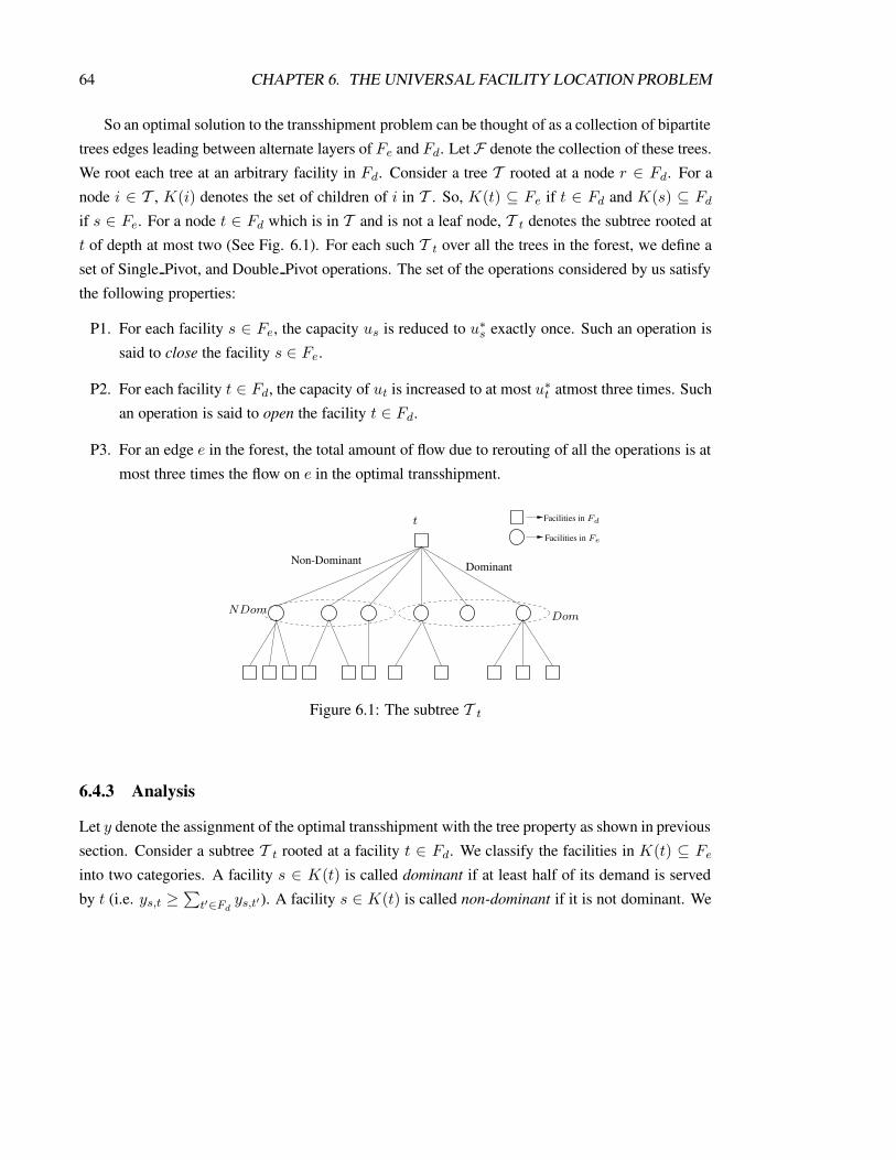
64 CHAPTER 6. THE UNIVERSAL FACILITY LOCATION PROBLEM
So an optimal solution to the transshipment problem can be thought of as a collection of bipartite
trees edges leading between alternate layers of Fe and Fd. LetF denote the collection of these trees.
We root each tree at an arbitrary facility in Fd. Consider a tree T rooted at a node r ∈ Fd. For a
node i ∈ T , K(i) denotes the set of children of i in T . So, K(t) ⊆ Fe if t ∈ Fd and K(s) ⊆ Fd
if s ∈ Fe. For a node t ∈ Fd which is in T and is not a leaf node, T t denotes the subtree rooted at
t of depth at most two (See Fig. 6.1). For each such T t over all the trees in the forest, we define a
set of Single Pivot, and Double Pivot operations. The set of the operations considered by us satisfy
the following properties:
P1. For each facility s ∈ Fe, the capacity us is reduced to u∗s exactly once. Such an operation is
said to close the facility s ∈ Fe.
P2. For each facility t ∈ Fd, the capacity of ut is increased to at most u∗t atmost three times. Such
an operation is said to open the facility t ∈ Fd.
P3. For an edge e in the forest, the total amount of flow due to rerouting of all the operations is at
most three times the flow on e in the optimal transshipment.
Facilities in Fd
Facilities in Fe
NDomDom
Dominant
t
Non-Dominant
Figure 6.1: The subtree T t
6.4.3 Analysis
Let y denote the assignment of the optimal transshipment with the tree property as shown in previous
section. Consider a subtree T t rooted at a facility t ∈ Fd. We classify the facilities in K(t) ⊆ Fe
into two categories. A facility s ∈ K(t) is called dominant if at least half of its demand is served
by t (i.e. ys,t ≥∑
t′∈Fdys,t′). A facility s ∈ K(t) is called non-dominant if it is not dominant. We

6.4. LOCALITY GAP 65
denote the set of dominant facilities by Dom, and the set of non-dominant facilities by NDom(See
Fig. 6.1). Further, we order the facilities in NDom by the non-decreasing order of the demand
served by t. If there are k facilities in NDom they are ordered s1, s2, . . . , sk such that ys1,t ≤ys2,t ≤ . . . ≤ ysk,t(See Fig. 6.2).
K(NDom)
Facilities in Fd
Facilities in Fe
t
Dom s1 s2 . . . si si+1 . . .sk
t
NDom
K(Dom)
Figure 6.2: Reassigning the demand for the Single Pivot, and Double Pivot operations.
We consider the operation Double Pivot(t, sk,∆1,∆2) in which we open {t} ∪ K(Dom) ∪K(sk) and close Dom ∪ {sk}. We route the excess of Dom via t to {t} ∪K(Dom). We route the
excess of sk via sk to {t} ∪K(sk). In particular the vectors are set as follows. ∆1i∈Dom = u∗
i − ui
(this is negative as i shrinks or closes), ∆1i∈K(Dom) = u∗
i − ui, ∆1t =
∑
i∈Dom yi,t (all these are
positive) and zero for other facilities. The pivot for this vector is t. We set ∆2sk
= u∗sk−usk
(negative
as sk shrinks/closes), ∆2t = ysk,t, ∆2
i∈K(sk) = u∗i − ui (positive), and zero for other facilities. We
set sk to be the pivot for this vector. It is easy to see that this is a feasible Double Pivot operation.
Since we are opening t in the above operation, it has sufficient capacity to take a demand of yi,t
for i ∈ Ndom \ {sk} as well. So, one could be tempted to reroute the excess of these facilities in
NDom by opening K(NDom \ {sk}). But, if there is a facility si ∈ K(NDom \ {sk}) such that
ysi,K(si) is arbitrarily larger than ysi,{t,sk} then, pivoting the flow ysi,K(si) via either t or sk could
violate property P3 mentioned in previous section. So, just one Double Pivot is not sufficient to
bound the facility costs of NDom \ sk. We bound the facility cost of the facilities in Ndom \ {sk}by defining a set of Single Pivot operations.
For each facility si ∈ NDom \ sk, we consider a Single Pivot(si,∆) operation. We set the
capacity of si to its capacity in S∗ (i.e, si is closed) and set the capacities of the facilities in K(si)∪K(si+1) to at most capacities in S∗ (i.e, open them). The vector ∆ is defined as follows. For each
facility l ∈ K(si), ∆l = ysi,l. For each facility l ∈ K(si+1), ∆l = ysi+1,l. For si, ∆si= u∗
si−usi
.
The facility si is the pivot for this operation. Clearly, rerouting of the demand from si to K(si)
is feasible. By the sorted order of the facilities in NDom and the fact that si+1 is non-dominating

66 CHAPTER 6. THE UNIVERSAL FACILITY LOCATION PROBLEM
means that ysi,t ≤ ysi+1,t ≤ ysi+1,K(si+1). Therefore, the routing of the the demand ysi,t to K(si+1)
is feasible and does not violate property P3 of the previous section.
This completes the set of operations performed on each subtree as defined in section 6.4.2. For
a subtree T t, each facility in K(t) is closed exactly once and each facility in {t} ∪ K(Dom) is
opened exactly once. Each facility in K(NDom) is opened exactly twice.
Lemma 6.4.4 Each facility i ∈ Fd is opened (i.e, its capacity is increased to u∗i ) at most three
times.
Proof. If a facility r ∈ Fd is the root of a tree, then it is considered in operations of the subtree
T r only. Consider a facility t ∈ Fd in a tree T rooted at r 6= t. Let t′ ∈ Fd be the facility such
that t ∈ K(K(t′)). If t is a leaf, then it is considered in the operations of only one subtree T t′ .Otherwise, it is considered in operations corresponding to two subtrees T t, and T t′ . As a part of
operations defined for T t′ , it can be opened at most twice. As part of operations defined for T t, it
is opened once.
Let the flow across an edge e ∈ F in the optimal transshipment be given by ye.
Lemma 6.4.5 For each edge e ∈ F , the amount of flow sent across e due to all the operations is at
most three times the flow across it in the optimal transshipment (i.e, 3 · ye).
Proof. Let Ed denote the set of edges which connect dominant facilities to their children. Consider
an edge e ∈ Ed. The Double Pivot operation which sends a flow of ye across e is the only operation
which sends flow through e. Let En denote the edges which connect non-dominant facilities to their
children. Consider an edge e ∈ En connected to a non-dominant facility si. In the Single Pivot
operation pivoted at si, the flow sent along e is equal to ye. In the Single Pivot operation pivoted
at si−1, the flow along e is at most ye, thus bounding the flow along e by 2 · ye. This also holds
for edges connecting non-dominant facilities to their parent. Finally, consider the set of edges
connecting dominant facilities to their parent. Let e be an edge which connects the root of a subtree
T t to its dominant facilities. The Double Pivot operations sends the flow of K(Dom) back and
forth along e before sending them to K(Dom) (Refer to Figure 6.2). As the flow to K(Dom) is at
most equal to the flow from Dom to t (i.e, ye), this flow is at most 2 · ye. The Double Pivot also
sends a flow of ye to t. Thus, the flow along e due to the operations is at most three times its flow in
the solution. As we have covered all edges, the lemma is true.
Lemma 6.4.6 The facility cost of the solution S is at most Cf (S) ≤ 3.Cf (S∗)+3(Cs(S)+Cs(S∗)).

6.4. LOCALITY GAP 67
Proof. The change in cost due to each of the operations is non-negative as S is a local optimum with
respect to these operations. Let CHG denote the set of facilities whose capacities change because
of a Single Pivot(s,∆) operation. It is easy to see that,
∑
i∈CHGGi(u
∗i − ui) +
∑
i∈CHGcsi.|∆i| ≥ 0
Let CHG1 and CHG2 denote the set of facilities whose capacities change because of the two pivot
operations in Double Pivot(s1, s2,∆1,∆2). It is easy to see that,
∑
i∈CHG1∪CHG2
Gi(u∗i − ui) +
∑
i∈CHG1
cs1i.|∆1i |+
∑
i∈CHG2
cs2i.|∆2i | ≥ 0
From lemmas 6.4.4 and 6.4.5 it is clear that, adding equations of the form 6.4.3 and 6.4.3 for all the
Single Pivot and Double Pivot operations, we get
3∑
i∈Fd
(Gi(u∗i )−Gi(ui)) + 3
∑
s,t
cstys,t ≥∑
i∈Fe
Gi(u∗i )−Gi(ui)
which gives us,
3Cf (S∗) + 3(Cs(S) + 3Cs(S∗)) ≥ Cf (S).
From lemma 6.4.1, we have
6Cf (S∗) + 6Cs(S∗) = 6C(S∗) ≥ Cf (S).
Lemmas 6.4.1 and 6.4.6 imply the following theorem.
Theorem 6.4.7 For any instance of UniFL, a locally optimum solution S with respect to add, Sin-
gle Pivot, and Double Pivot operations has a total cost C(S) ≤ 7.Cf (S∗) + 7.Cs(S∗) where S∗ is
any optimal solution to the UniFL instance.
Recently, we have proved that the techniques of Zhang et al. [59] can be combined with the Dou-
ble Pivot operation to show a locality gap of 6 for the UniFL problem [18]. Currently, this is the
best known approximation factor for the UniFL problem.

68 CHAPTER 6. THE UNIVERSAL FACILITY LOCATION PROBLEM

Chapter 7
The budget constrained k-medianproblem
In this chapter, we consider the Budget Constrained k-median problem defined in Section 2.1.6. We
propose a pre-processing algorithm followed by a local search heuristic. Our problem formulation
helps us to study the effectiveness of local search for bicriteria optimization problems.
7.1 Motivation
The k-median, and k-center measures in facility location optimize contrasting objective functions.
In the k-median problem, the goal is to minimize the average service cost of the set of clients. On
the other hand, the k-center objective function is a fairness measure, i.e, it minimizes the maximum
distance of a client to its nearest facility. So, while the challenge in the k-median problem is to
minimize the L1 norm, the challenge in the k-center problem is to minimize the L∞ norm. This
contrast in the objective functions can be exploited to show that a simultaneous approximation of
both the measures within constant factors is not possible. Consider the example shown in Figure
7.1. A and B are points representing clusters of demand n. Z is a point with a unit demand. Thedistance between A and B is 1, while the distance of Z from both A and B is
√n. Let k be 2. The
optimal solution for the k-median measure picks A and B as the facilities and has a cost of√
n. Its
k-center cost is√
n. The optimal solution for the k-center measure picks a facility at Z , and one at
either A or B and has a cost of 1. Its k-median cost is n. So, any choice of 2 facilities exceeds the
optimal value of one of the measures by a factor√
n.
69

70 CHAPTER 7. THE BUDGET CONSTRAINED K-MEDIAN PROBLEM
Z
√n
√n
1
A
B
Figure 7.1: Example where approximating 2-median and 2-center within constant factors is notpossible.
Cli
.
...
..
pn/X−1
p1
p2
pi
X
1p0
Cln/X
Cl1
Cl2Cl3
Figure 7.2: Sometimes medians can be fair to all clients.

7.1. MOTIVATION 71
However, there are situations when obtaining good solutions with respect to both k-median
and k-center measures is possible and desirable. Consider the example shown in Figure 7.2. The
figure shows n/X clusters {Cl1, . . . , Cln/X} of size X which are at a distance of 1 from a central
point p0. There are n/X − 1 points {p1, . . . , pn/X−1} at a distance of X from one of the clusters
as shown in the figure. Let k be n/X . Suppose we pick the center of all the clusters, namely,
CH1 = {Cl1, . . . , Cln/X}. The k-median cost of CH1 is n and k-center cost is X . Instead, we
could pick CH2 = {p0, p1, . . . , pn/X−1} as the k facilities. The k-median cost of CH2 is also n.
On the brighter side, the k-center cost of CH2 is 1. This example abstracts the problem of facility
location in a city with many satellite towns around it. Although the natural answer in this case
is quite intuitive, many computational problems with this requirement need specialized heuristics.
With these motivations, we formulate the budget constrained k-median problem. In Section 2.1.6,
we formulated the problem as follows.
• Input: The set of clients C . The distances between clients in C satisfy metric properties.
Input also consists of an integer k and a budget B. For a client j ∈ C and a set S ⊆ C ,
ds(j, S) denotes mini∈S
cij .
• Validity: A valid solution S ⊆ C is such that, (|S| ≤ k) ∧ (∀ i ∈ C : ds(i, S) ≤ B).
• Assumption: The input has at least one valid solution.
• Output: A valid solution S such that∑
i∈C ds(i, S) is minimized.
We have surveyed the existing results on the k-median problem in Chapter 3. Gonzales [19]
gave a farthest point greedy heuristic for the k-center problem, which runs in O(nk) time and gives
a 2-approximation. Hochbaum and Shmoys [24] also gave a 2-approximation for this problem
using a generic technique applicable to a class of “bottleneck” problems. They also show that no
polynomial time algorithm can approximate the k-center problem to a factor better than 2 unless
P = NP . The primal-dual based Lagrangian relaxation technique of Jain and Vazirani [27] can
be modified to get a (6, 9) approximation algorithm for the budget constrained k-median problem.
Essentially, the input is pruned to contain only those edges whose lengths are within the budget.
However, we study this problem to show that the local search technique can be used in bi-criteria
optimization problems with an appropriate pre-processing stage. The budget represents a set of
constraints on the service cost of each client. Local search techniques for constraint programming
(CP) problems with optimization goals have also been studied. Travelling salesman problem with

72 CHAPTER 7. THE BUDGET CONSTRAINED K-MEDIAN PROBLEM
time windows (TSPTW) is a typical example of such problems. Pesant and Gendreau [48] integrate
branch and bound technique with local search to report empirical results on the TSPTW problem.
Our technique gives rise to the question of applying local search in CP problems using appropriate
pre-processing techniques.
Our algorithm has two phases: a preprocessing phase and a local search phase. In the prepro-
cessing phase, we partition the set of clients C into mutually disjoint sets C1, C2, . . . Cl such that
the diameter of each Ci is within a constant times the budget B. Furthermore, any valid solution is
guaranteed to open a certain minimum number of facilities inside each of C1, . . . , Cl. In the local
search space, we run the single swap heuristic for the k-median problem with the restriction that
it explores only those solutions which open at least one facility in each of the Ci’s. We call it as
restricted local search heuristic. We call a solution S ⊆ C as fine with respect to the partition, if
it opens at least one facility in each of the Cis. Our goal is to use the analysis technique presented
in Section 3.3 to the modified procedure to obtain a constant factor approximation for the k-median
measure. In this chapter, we show that such an approach is feasible.
7.2 A simple scheme that fails
As there is atleast one valid solution, we consider the following iterative algorithm to cluster the set
of clients. In iteration i, pick an unclustered client j ∈ C . Create a new cluster Ci consisting of j
and all unclustered clients within a distance of 2 ·B from j. The proof of the factor 2 approximation
algorithm for the k-center given by Hochbaum and Shmoys [24] guarantees that we get atmost k
clusters. Let these clusters be C1, . . . , Cl, l ≤ k.
Let us consider the restricted local search with C1, . . . , Cl as the partition of the client set. Let S
denote a local minimum computed by the restricted local search. Let O denote the optimal solution
for the budget constrained k-median problem. Note that, our construction ensures that every client
has an open facility within a distance of 4 · B. We would like to apply the analysis of k-median
problem presented in Section 3.3 to bound the service cost of S. The highlights of the k-median
analysis were:
P1. Swap every 1-bad facility with the optimum facility that it captures.
P2. Swap the rest of the optimum facilities with good facilities such that each good facility is
considered in atmost two swaps.

7.3. COMPUTING A BOUNDED DIAMETER PARTITION 73
However, in case of restricted local search, we can consider only those swaps which result in a fine
solution with respect to C1, . . . , Cl. This restriction prevents us from considering the following
swaps which were essential in the k-median analysis. As always, we denote the local optimum
solution by S and the optimum by O.
B1. Consider a 1-bad facility s ∈ S which captures o ∈ O. Suppose s is the only facility opened
inside a cluster Ci and o 6∈ Ci then, the swap 〈s, o〉 is not allowed as the resulting solution is
not a fine solution.
B2. Consider a good facility s ∈ S which is the only facility opened inside a cluster Ci. Clearly,
s can be swapped with only those facilities in optimum which are inside Ci.
The limitations B1 and B2 prevent us from applying the analysis of the k-median problem to
bound the service cost of S in terms of the service cost of O. In fact, the idea cannot be made
to work even by computing the clusters such that any valid solution is guaranteed to open at least
2 facilities in each Ci. We first observe that a set of swaps which satisfy the following relaxed
constraints is sufficient to obtain a constant factor approximation:
P3. All the optimum facilities can be considered in exactly one swap while ensuring that no
facilities in S is considered in more than a constant number of swaps.
P4. If a swap 〈s, o〉 is considered, then the facility s does not capture any facility o ′ 6= o.
The observations made in B1, B2, P3, and P4 motivate us to compute a bounded diameter partition.
Informally, we compute a partition in which either a cluster is far from other clusters or any valid
solution is guaranteed to open atleast three facilities inside it. In the rest of our discussion, we use
the terms cluster and region interchangeably. The diameter of each region is bounded by constant
times the budget B. We formalize these ideas in the next section.
7.3 Computing a Bounded Diameter Partition
In this section, we give a procedure which computes a bounded diameter partition. This construction
is used to formulate a generalized notion of bounded diameter partition. We first try to cover all
the clients by regions in which any valid solution is guaranteed to open at least three facilities. The
clients not covered by such regions are covered by regions which are far from others. We choose our
parameters such that a local minimum of restricted local search has at most k/3 limitations of type

74 CHAPTER 7. THE BUDGET CONSTRAINED K-MEDIAN PROBLEM
B1 and B2. Our partitioning is iterative and begins with all the clients classified as “uncovered”.
We use R’s to denote clusters or regions which are essentially subsets of the set of clients. We
use the term envelope of radius r around a region R to denote the set of clients {j ∈ C|((j 6∈R) ∧ (ds(j, R) ≤ r))}. For a client j ∈ C , B(j, r) denotes the set of all clients within a distance of
r from j.
7.3.1 Triplet Phase
Initially, we form regions in which any valid solution is guaranteed to open at least 3 facilities. We
call such a region as triplet region. A triplet region T is defined by three clients p1, p2, and p3 such
that B(p1, B), B(p2, B), B(p3, B) are disjoint and one of the points, say p1, is at a distance of at
most 6 ·B from both p2, p3. Figure 7.3 shows a triplet region. The set of clients assigned to a triplet
region is a subset of the set of clients in the union of balls of radius 3 ·B around p1, p2, and p3. The
set of all clients in the balls of radius B around p1, p2, and p3 is said to be the core of such a triplet
region and denoted by Core(T ). So, the maximum distance of a client inside a triplet region from
its core is at most 16 · B. A maximal set of triplet of regions can be computed iteratively. In each
B
p2
p1
p3
3 · B
Figure 7.3: Illustration of a triplet region
iteration, three uncovered clients which can form a triplet region are identified. Suppose pi1, pi2, pi3
are the points satisfying triplet condition in iteration i. We mark all the uncovered clients inside
∪q∈{1,2,3}B(piq, 3 · B) as covered and assign it to the ith triplet region, Ti. Note that, some of
the clients in ∪q∈{1,2,3}B(piq, 3 · B) may have been assigned to triplet regions formed in earlier
iterations. Also, note that any of pi1, pi2, pi3 could be close to a triplet region formed in previous
iterations. So, Core(Ti) need not be a subset of Ti. We terminate the process when it is not possible
to find three uncovered clients which satisfy triplet condition. It is easy to see that if T1 and T2 are

7.3. COMPUTING A BOUNDED DIAMETER PARTITION 75
two triplet regions identified by this iterative process, then Core(T1)∩Core(T2) = ∅. We call this
phase as the triplet phase. Clearly, it can be implemented in O(kn3) time.
7.3.2 Doublet Phase
Note that the triplet phase may not cover all the clients. We try to cover the remaining clients by
regions in which any valid solution is guaranteed to open at least 2 facilities called doublet region.
A doublet region D is defined by two clients p1, and p2 such that 2B < ds(p1, p2) < 4 · B and
there does not exist an uncovered client p3 such that p1, p2, and p3 form a triplet region. The set ofclients assigned to a doublet region is a subset of clients in the union of balls of radius 2 ·B around
p1, and p2. Figure 7.4(A) shows a doublet region.
Envolope of 4 · B around the boundary does not intersect
(A) (B)
p1 p2
p1 p2
2 · B < d < 4 · B
2 · BBB 2 · B
2 · B < d < 4 · B
any triplet region.
Figure 7.4: Illustration of a doublet region
Lemma 7.3.1 After the triplet phase, the envelope of radius 4 · B around a doublet region defined
by two uncovered clients does not contain any uncovered clients.
Proof. Suppose an uncovered client p3 exists in the envelope of radius 4 · B around the doublet
region defined by p1, and p2. The clients p1, p2, and p3 define a triplet region and the set of triplet
regions formed by triplet phase is not maximal. This is contrary to the fact that the triplet phase
terminated. Hence, the envelope of 4 · B around any doublet region is free of uncovered clients.
Let D1 be a doublet region defined by two uncovered clients (p1, p2) after the triplet phase. Let
D2 be a doublet region defined by two uncovered clients (p3, p4) such that {p1, p2} ∩ {p3, p4} = ∅.Let U1 denote the set of uncovered clients in the union of balls of radius 2 ·B around p1, p2. Let U2
be defined similarly for p3, p4. The proof for Lemma 7.3.1 implies the following lemma.

76 CHAPTER 7. THE BUDGET CONSTRAINED K-MEDIAN PROBLEM
Lemma 7.3.2 The distance of the two sets U1, U2 defined by maxi∈U1,j∈U2(cij) is at least 4 ·B.
We now form a set of doublet regions in an iterative manner. At each iteration, we find two
points p1, p2 which define a doublet region. Let D be the set of uncovered clients in the union of
balls of radius 2 · B around p1, p2. If the envelope of radius 4 · B around D intersects a triplet
region T discovered in the triplet phase, then all the clients in D are marked covered and assigned
to T . If the envelope intersects many triplet regions, then one of them is chosen arbitrarily. If the
envelope does not intersect any of the triplet regions, then the doublet region is called an isolated
doublet region (Figure 7.4(B)). All the clients in D are marked covered and assigned to the isolated
doublet region. The core of an isolated doublet region denoted by Core(D), contains all the clients
assigned to it. Lemma 7.3.2 implies that no two doublet regions are attached to a triplet region
through a chain. In other words, if D1 and D2 are two doublet regions which got merged with atriplet region T formed in triplet phase, then both D1 and D2 intersect the envelope of radius 4 · Baround T . This phase is called the doublet phase.
7.3.3 Singlet Phase
So far, we have covered a subset of the set of clients by triplet regions, and isolated doublet regions.
We cover the remaining uncovered clients in the following manner. After the doublet phase, the
distance between two uncovered clients is either less than 2 · B or greater than 4 · B. Each set of
uncovered clients which are at a distance of less than 2 ·B from each other form a singlet region as
shown in Figure 7.5.
less than 4 · B.
merged to a triplet region
Clusters of diameter
Isolated singleton regions
Points covered by tripletregions already forned.
is empty.
2 · B
4 · B
2 · B
4 · BThe envelope of 4 · B around
Singleton region which gets
Figure 7.5: Illustration of a singlet region

7.3. COMPUTING A BOUNDED DIAMETER PARTITION 77
Lemma 7.3.3 After the doublet phase, the envelope of radius 4 ·B around a singlet region does not
intersect an isolated doublet region or a doublet region which got merged with a triplet region.
Proof. Similar to the proof of 7.3.1.
However, the envelope of radius 4 ·B around a singlet region may intersect a triplet region T . If
such is the case, then we mark all the clients in the singlet region as covered and assign to the triplet
region T . Otherwise, such a singlet region is called an isolated singlet region. All the clients insidean isolated singlet region are covered and assigned to it. The core of an isolated singlet region is the
set of all clients assigned to it. Thus, we have covered all the clients by assigning to triplet regions,
isolated doublet regions, and isolated singlet regions.
Lemma 7.3.4 The partition obtained by the above process is such that, the maximum distance of a
client from the core of its region is at most 28 · B.
Proof. The upper bound on the diameter of a region is the diameter of a region formed by merging adoublet region with a triplet region. The diameter of a triplet region in the triplet phase with respect
to its core is 16 · B. The diameter of a doublet region is 8 · B and they can be separated by at most
4 ·B. Thus, the diameter of a region with respect to its core is bounded by 28 · B.
7.3.4 Generalization
We have shown how to construct a partition in which the diameter of each region with respect to its
core is at most 28 · B. Each region is either a triplet region, or an isolated region. The cores of any
two regions are disjoint. This idea can be generalized to define (a, b) partition where a is a constantgreater than 2 and b is the maximum diameter of a region with respect to its core.
Consider an input (C, k,B) to the budget constrained k-median problem, where C is the set of
clients, k is an integer, and B is the budget on the quality of the k-center solution. For a client j,
we denote the set of all clients within a distance of r by B(j, r). We now define a (a, b)-partition of
the set of clients. Intuitively, the idea is to partition the set of clients into regions of radius at most
b ·B. Furthermore, for each region, any valid solution is guaranteed to open a facilities inside it, or
it is far from other regions. Formally, a partition of the set of clients C into regions R1, . . . , Rl is
called (a, b)-partition if the following properties hold:
1. Rp 6= ∅ and Rp ∩Rq = ∅ for all p 6= q,

78 CHAPTER 7. THE BUDGET CONSTRAINED K-MEDIAN PROBLEM
2. For a region Rp (p = 1, . . . , l),
(a) either, we can fix a set Rap = {j1, . . . ja} ⊆ Rp such that, if ((jx, jy ∈ Ra
p)∧ (jx 6= jy)),
then B(jx, B) ∩ B(jy, B) = ∅. Such a region is called a-populated region. The set
∪jx∈RapB(jx, B) is said to be the core of the a-populated region. Some of the clients in
the core of an a-populated region may belong to different regions.
(b) or, for any j ∈ C , j 6∈ Rp implies ds(j, Rp) = minj′∈Rpds(j, j′) > 4 · B. Let
{j1, . . . jw : w < a} ⊆ Rp be the maximum number of points such that B(jx, B)’s are
disjoint. This means that, for any client j ∈ Rp, ds(j, {B(j1, B), . . . ,B(jw, B)}) ≤2 · B. We call such a region as w-populated-isolated region. The core of an isolated
region is the entire region.
3. Furthermore, if Rp, Rq are two a-populated regions defined by Rap, R
aq , then ds(Ra
p, Raq ) >
2 ·B. This implies that the core of two a-populated regions do not intersect.
4. The maximum distance of a client from the core of its region is at most b · B.
Properties 2(a) and 4 ensure that any valid solution has to open at least a facilities inside the core
of an a-populated region. The preprocessing algorithm of the previous section gives a a (3, 28)
partition. It can be generalized to obtain a (K, 10K − 2) partition for any constant K by suitably
defining K-plet regions. The most straightforward implementation of K-plet regions will take
O(knK) time.
7.4 Restricted Local Search
The single-swap heuristic for the k-median problem presented in Section 3.3, starts with an arbitrary
set of size k and at each step considers doing a swap which improves the cost. The algorithm
terminates when a local minima is reached. Let R1, . . . , Rl denote the bounded diameter partition
computed by the preprocessing phase. The restricted local search mimics the k-median algorithm
while exploring only fine solutions, i.e, atleast one facility is opened inside each region. Refer to
Figure 7.6.
As always, cost(S) denotes the service cost of a solution S. An algorithm is said to be a (α, β)-
approximation if, for every instance of the problem, it opens a set of k facilities, denoted by S, such
that, the cost(S) is at most α times the cost of the optimal valid solution and the induced k-center
cost of S is at most βB. The main theorem we want to prove is:

7.5. ANALYSIS OF LOCALITY GAP 79
Algorithm Restricted Local Search.
1. S ← an arbitrary fine solution.2. While ∃ s ∈ S and s′ 6∈ S such that S − {s}+ {s′} is a fine solution
and cost(S − {s}+ {s′}) < cost(S),do S ← S − {s}+ {s′}.
3. return S.
Figure 7.6: Restricted Local Search
Theorem 7.4.1 If the restricted local search algorithm in Figure 7.6 uses (a, b)-partition, it is a
(((5a − 2)/(a − 2)) + ε, b)-approximation algorithm for budget constrained k-median problem.
7.5 Analysis of Locality Gap
In this section, we prove the theorem stated in 7.4.1. Here, we assume that a suitable (a, b)-partition
is obtained, for some a > 2. We analyze the locality gap of the restricted local search. As always,
the local optimum solution output by the restricted local search is denoted by S and O denotes an
optimum solution. We reuse all the notations introduced in the analysis of the k-median problem
and consider a 1-1 and onto function π : NO(o)→ NO(o) as defined in Section 3.3 for each facility
o ∈ O.
The following simple observation can be made about a facility s ∈ S if it is the only facility
opened inside an isolated region.
Lemma 7.5.1 If a facility s ∈ S is the only facility opened inside an isolated region Ri, then it has
to capture at least one facility o ∈ O which is inside Ri.
Proof. Suppose s ∈ S is the only facility inside a x-populated isolated region Ri. Any valid
solution has to open a facility within a distance of B from s, say o ∈ O. By definition of isolated
region, o ∈ Ri. So, all the clients inside NO(o) are within a distance of 2 · B from s. Since the
region Ri is isolated, if c 6∈ Ri, then its distance from s is greater than 4 · B. So, its distance from
clients in NO(o) is greater than 2 ·B. So, s is the nearest facility to all clients in NO(o) and captures
o.
The main idea is to define a set of k swaps such that, each swap results in a fine solution. We
then use our standard technique of proving the locality gap by writing inequalities corresponding to

80 CHAPTER 7. THE BUDGET CONSTRAINED K-MEDIAN PROBLEM
each swap. As in the analysis of the k-median heuristic, we would like to swap a 1-bad facility with
the optimum facility that it captures. Also, we do not include a (2+)-bad facility in any swap. We
classify the facilities in S depending on the restrictions they impose on considering single swaps.
Consider a facility s ∈ S which captures exactly one facility o ∈ O. If s is the only facility
inside the core of an a-populated region Ri and o is not in the core of Ri, then the swap 〈s, o〉 is not
feasible as the resulting solution is not a fine solution. Such a facility s is called constrained 1-bad
facility. Let Bc1 denote the set of constrained 1-bad facilities. Let bc
1 = |BC1 |. The rest of the 1-bad
facilities are called unconstrained 1-bad and denoted by Bu1 . Let bu
1 = |Bu1 |. We use B2+ to denote
the set of (2+)− bad facilities. Let b2+ = |B2+|.Consider a good facility s ∈ S. Suppose it is the only facility opened by S inside the core of a
region Ri. Clearly, s can be considered can be swapped with only those facilities in the optimum
which are inside the core of the region Ri. We call such a good facility as constrained good facility
and denote the set of constrained good facilities by Gc. Let gc = |Gc|. Rest of the good facilities
are called unconstrained good facilities and can be considered in any swap and denoted by Gu. Let
gu = |Gu|.By lemma 7.5.1, constrained 1-bad facilities and constrained good facilities can be present in
a-populated regions only. We consider the following swaps.
• Suppose s is an unconstrained 1-bad facility capturing o, then we consider the swap 〈s, o〉.
• The remaining k − bu1 facilities of O are considered in swaps with only unconstrained good
facilities. Each unconstrained good facilities is considered in (k − bu1)/gu swaps.
The swaps considered above satisfy the following properties.
1. Each o ∈ O is considered in exactly one swap.
2. A facility s ∈ S which captures more than one facility in O is not considered in any swap.
3. Each good facility s ∈ S is considered in at most (k − bu1)/gu swaps.
4. If swap 〈s, o〉 is considered then facility s does not capture any facility o ′ 6= o.
We claim that gu ≥ (k−bu1 )(a−2)2a . Suppose this is true, then (k − bu
1)/gu ≤ 2a/(a − 2). The
proof of our claim follows.
After we consider the swaps of all unconstrained 1-bad facilities, we are left with k1 = k − bu1
optimum facilities to be considered for swaps. The number of constrained 1-bad facilities, and

7.5. ANALYSIS OF LOCALITY GAP 81
constrained good facilities is bounded by the maximum number of a-populated regions required to
cover k1 facilities.
gc + bc1 ≤ k1/a (7.1)
As we are left with exactly k1 facilities in our solution which have not been considered so far:
gc + gu + bc1 + b2+ = k1 (7.2)
Clearly, the number of facilities captured by bad facilities cannot exceed k1.
bc1 + 2b2+ ≤ k1 (7.3)
Simple manipulations show that:
2gc + 2gu + 2bc1 + 2b2+ = 2k1{multiplying (7.2) by 2 }
2gc + 2gu + bc1 ≥ k1{by substituting (7.3) }
gc + 2gu ≥ k1(a− 1)
a{ Substituting (7.1) }
2gu ≥ k1(a− 2)
a{Substituting (7.1) }
gu ≥ k1(a− 2)
2a(7.4)
o o′
s′
s
Sπ(j′)
Oπ(j′)Oj′Oj
SjSj′
π(j′)j j′
Figure 7.7: Reassigning the clients in NS(s) ∪NO(o).
We now analyze these swaps one by one. Consider a swap 〈s, o〉. We place an upper bound onthe increase in the cost due to this swap by reassigning the clients in NS(s)∪NO(o) to the facilities
in S − s + o as follows (Figure 7.7). The clients j ∈ NO(o) are now assigned to o. Consider a

82 CHAPTER 7. THE BUDGET CONSTRAINED K-MEDIAN PROBLEM
client j′ ∈ N o′s , for o′ 6= o. As s does not capture o′, by the property of our mapping function π, we
have that π(j ′) 6∈ NS(s). Let π(j ′) ∈ NS(s′). Note that the distance that the client j ′ travels to the
nearest facility in S−s+o is at most cj′s′ . From triangle inequality, cj′s′ ≤ cj′o′+cπ(j′)o′+cπ(j′)s′ =
Oj′ + Oπ(j′) + Sπ(j′). The clients which do not belong to NS(s)∪NO(o) continue to be served by
the same facility.
Therefore,
∑
j∈NO(o)
(Oj − Sj) +∑
j∈NS(s),
j 6∈NO(o)
(Oj + Oπ(j) + Sπ(j) − Sj) ≥ 0. (7.5)
As each facility o ∈ O is considered in exactly one swap, the first term of inequality (7.5) added
over all k swaps gives exactly cost(O)−cost(S). For the second term, we will use the fact that each
s ∈ S is considered in at most 2a/(a − 2) swaps. Since Sj is the shortest distance from client j to
a facility in S, using triangle inequality we get: Oj + Oπ(j) + Sπ(j) ≥ Sj . Thus the second term ofinequality (7.5) added over all k swaps is no greater than 2a/(a−2)
∑
j∈C(Oj+Oπ(j)+Sπ(j)−Sj).
But since π is a 1-1 and onto mapping,∑
j∈C Oj =∑
j∈C Oπ(j) = cost(O) and∑
j∈C(Sπ(j) −Sj) = 0. Thus, 2a/(a−2)
∑
j∈C(Oj +Oπ(j) +Sπ(j)−Sj) = 4a/(a−2) ·cost(O). Combining the
two terms we get, cost(O)−cost(S)+4a/(a−2)·cost(O) ≥ 0. Thus, (5a−2)/(a−2)·Cost(O) ≥Cost(S). This proves the theorem 7.4.1.
Theorem 7.5.2 There exists a (13 + ε, 28) approximation algorithm for the budgeted k-median
problem.
Proof. The construction given in Section 7.3 gives a (3, 28) partition. From Theorem 7.4.1, it
follows that there exists a (13+ε, 28) approximation algorithm for the budgeted k-median problem.
More generally, using a preprocessing stage which computes K-plet regions, we can get a (5K −2/K − 2, 10K − 2) approximation algorithm for any constant K .

Chapter 8
Conclusions and open problems
In this thesis, we showed the power of local search for approximating facility location problems.
Local search is widely used by programmers for their simplicity in understanding and implementing.
The results shown here go towards explaining the success of local search heuristics. The study of
local search for different combinatorial optimization is desirable not just to obtain better algorithms,
but also to better understand their relation with complexity of computational problems.
The algorithms presented in this thesis have the same iterative structure. The local operations
vary depending on the problem. The set of local operations needed to prove the locality gaps for
different problems also bear a strong resemblance to the way the heuristics are strengthened when
different pathological cases emerge. The approximation ratio achieved for the k-median problem
remains the best known. So far, local search is the only known technique to yield non-trivial approx-
imation ratios for capacitated versions with hard capacities. We also present a local search heuristic
for the budget constrained k-median problem which opens the possibility of local search heuristics
for bi-criteria and constraint satisfaction optimization problems.
Along the line of the results presented in this thesis, several possibilities emerge. Most important
among them is, does there exist a characterization of the games for which the price of anarchy can
be analyzed via locality gap? Local search analyzes of combinatorial optimization problems with
different covering/packing constraints may help obtain better characterization of complexity classes
as presented in Section 2.3. Can the power of local search be improved by intelligent preprocessing
as shown in Chapter 7?
In the context of facility location problems, several challenges remain open. They are:
1. Most important open problem in facility location is the generalized median problem. In the
83

84 CHAPTER 8. CONCLUSIONS AND OPEN PROBLEMS
generalized median problem, the facility costs of the facilities are non-uniform. There is a
fixed budget available for opening the facilities. The goal is to open a set of facilities whose
total cost is within the budget and the service cost is minimized. The k-median problem
is a special case of the generalized median problem in which the facility costs are uniform.
No non-trivial approximation ratio is known for this problem. As in the case of capacitated
facility location with hard capacities, it would be interesting to see if a local search technique
gives the first approximation algorithm for this problem.
2. Another important problem in facility location is to get better estimates of lower bounds for
capacitated facility location instances via linear programs. This may eventually help to design
approximation algorithm for capacitated facility location with hard capacities based on linear
programming. Some preliminary results in this direction dealing with special cases of capac-itated facility location with hard capacities is presented by Levi, Shmoys, and Swamy [36].
3. Approximation algorithms for the capacitated versions of the k-median problem, fault tolerant
facility location [22, 54], and facility location with outliers [11] would also be interesting.

Bibliography
[1] A. Archer, R. Rajagopalan, and D. Shmoys. Lagrangian relaxation for the k-median problem:
new insights and continuity properties. In Proceedings of 11th Annual European Symposium
on Algorithms, pages 31–42, 2003.
[2] E. Arkin and R. Hassin. On local search for weighted k-set packing. Mathematics of Opera-
tions Research, 23(3):640–648, 1998.
[3] V. Arya, N. Garg, R. Khandekar, V. Pandit, A. Meyerson, and K. Munagala. Local search
heuristics for k-median, and facility location problems. Siam Journal of Computing, 33:544–
562, 2004.
[4] G. Ausiello and M. Protasi. Local search, reducibility and approximability of NP-optimization
problems. Information Processing Letters, 54:73–79, 1995.
[5] Y. Bartal. Probabilistic approximations of metric spaces and its algorithmic applications. In
Proceedings of the 37th IEEE Symposium on Foundations of Computer Science, pages 184–
193, 1996.
[6] Y. Bartal. On approximating arbitrary metrics by tree metrics. In Proceedings of the 30th
Annual ACM Symposium on Theory of Computing, pages 161–168, 1998.
[7] B. Chandra, H. Karloff, and C. Tovey. New results on the old k-opt algorithm for the TSP.
In Proceedings of the 5th Annual ACM-SIAM Symposium on Discrete Algorithms, pages 150–
159, 1994.
[8] M. Charikar, C. Chekuri, A. Goel, and S. Guha. Rounding via trees: deterministic approxima-
tion algorithms for group steiner trees and k-median. In Proceedings of the 30th Annual ACM
Sympsium on Theory of Computing, pages 114–123, 1998.
85

86 BIBLIOGRAPHY
[9] M. Charikar and S. Guha. Improved combinatorial algorithms for the facility location and k-
median problems. In Proceedings of the 40th Annual Symposium on Foundations of Computer
Science, pages 378–388, 1999.
[10] M. Charikar, S. Guha, E. Tardos, and D. Shmoys. A constant-factor approximation algorithm
for the k-median problem. Journal of Computer and System Sciences, 65:129–149, 2002.
[11] M. Charikar, S. Khuller, D. Mount, and G. Narasimhan. Algorithms for facility location prob-
lems with outliers. In Proceedings of the 12th Annual ACM-SIAM Symposium on Discrete
Algorithms, pages 642–651, 2001.
[12] F. Chudak. Improved approximation algorithms for uncapacitated facility location problem. In
Proceedings of the 6th Conference on Integer Programming and Combinatorial Optimization,
pages 182–194, 1998.
[13] F. Chudak and D. Shmoys. Improved approximation algorithms for capacitated facility loca-
tion problem. In Proceedings of the 10th Annual ACM-SIAM Symposium on Discrete Algo-
rithms, pages 875–876, 1999.
[14] E. Clarke. Multiparty pricing in public goods. Public Choice, pages 17–33, 1971.
[15] G. Cornuejols, G. Nemhauser, and L. Wolsey. The uncapacitated facility location problem. In
P. Mirchandani and R. Francis, editors, Discrete Location Theory. John Wiley and Sons, 1990.
[16] N. Devanur, N. Garg, R. Khandekar, V. Pandit, A. Saberi, and V. Vazirani. Price of anarchy,
locality gap, and a network service provider game. Submitted for publication, April 2004.
[17] M. Furer and B. Raghavachari. Approximating the minimum degree spanning tree to within
one from the optimal degree. In Proceedings of 3rd Annual ACM-SIAM Symposium on Dis-
crete Algorithms, pages 317–324, 1992.
[18] N. Garg, R. Khandekar, and V. Pandit. Improved approximation for the universal facility
location. In Proceedings of the 16th Annual ACM-SIAM Symposium on Discrete Algorithms,
January 2005.
[19] T. Gonzales. Clustering to minimize the maximum intercluster distance. Theoretical Computer
Science, 38:293–306, 1985.

BIBLIOGRAPHY 87
[20] T. Groves. Incentives in games. Econometrica, pages 617–631, 1973.
[21] S. Guha and S. Khuller. Greedy strikes back: improved facility location algorithms. In Pro-
ceedings of the 9th Annual ACM-SIAM Symposium on Discrete Algorithms, pages 649–657,
1998.
[22] S. Guha, A. Meyerson, and K. Munagala. Improved algorithms for fault tolerant facility lo-
cation. In Proceedings of the 12th Annual ACM-SIAM Symposium on Discrete Algorithms,
pages 636–641, 2001.
[23] D. S. Hochbaum. Heuristics for the fixed cost median problem. Mathematica Programming,
22:148–162, 1982.
[24] D.S. Hochbaum and D. Shmoys. A best possible heuristic for k-center problem. Mathematics
of Operations Research, 10:180–184, 1985.
[25] K. Jain, M. Mahdian, E. Markakis, A. Saberi, and V. Vazirani. Greedy facility location algo-
rithms analyzed using dual fitting factor revealing lp. To appear in the Journal of ACM.
[26] K. Jain, M. Mahdian, and A. Saberi. A new greedy approach for facility location problems. In
Proceedings of the 34th Annual ACM Symposium on Theory of Computing, 2002.
[27] K. Jain and V. Vazirani. Approximation algorithms for metric facility location and k-
median problems using the primal-dual schema and Lagrangian relaxation. Journal of ACM,
48(2):274–296, 2001.
[28] T. Kanungo, D. Mount, N. Netanyahu, C. Piatko, R. Silverman, and A. Wu. A local search
approximation algorithm for k-means clustering. In Proceedings of the 18th Annual ACM
Symposium on Computational Geometry, pages 10–18, 2002.
[29] S. Khanna, R. Motwani, M. Sudan, and U. Vazirani. On syntactic versus computational views
of approximability. Siam Journal of Computing, 28:1:164–191, 1999.
[30] S. Khuller, R. Bhatia, and R. Pless. On local search and placement of meters in networks. In
Proceedings of the 11th Annual ACM-SIAM Symposium on Discrete Algorithms, pages 319–
328, 2000.

88 BIBLIOGRAPHY
[31] J. Koneman and R. Ravi. A matter of degree: improved approximation algorithms for degree-
bounded minimum spanning trees. In Proceedings of the 32nd Annual ACM Symposium on
Theory of Computing, pages 537–546, 2000.
[32] M. Korupolu, C. Plaxton, and R. Rajaraman. Analysis of a local search heuristic for facility
location problems. Technical Report 98–30, DIMACS, 1998.
[33] M. Korupolu, C. Plaxton, and R. Rajaraman. Analysis of a local search heuristic for facility
location problems. In Proceedings of the 9th Annual ACM-SIAM Symposium on Discrete
Algorithms, 1998.
[34] E. Koutsoupias and C. Papadimitriou. Worst-case equilibria. In Proceedings of the 16th Annual
Symposium on Theoretical Aspects of Computer Science, pages 404–413, 1999.
[35] A. Kuehn and M. J. Hamuburger. A heuristic program for locating warehouses. Management
Sciences, 9:643–666, 1963.
[36] R. Levi, D. Shmoys, and C. Swamy. Lp based approximation algorithms for capacitated facil-
ity location. In Proceedings of the 10th Conference on Integer Programming and Combinato-
rial Optimization, 2004.
[37] J. Lin and J. Vitter. Approximation algorithms for geometric median problems. Information
Processing Letters, 44, 1992.
[38] J. Lin and J. Vitter. ε approximation with minimum packing constraint violation. In Proceed-
ings of 24th Annual ACM Symposium on Theory of Computing, pages 771–782, 1992.
[39] S. Lin and B. Kernigham. An effective heuristic algorithm for the traveling salesman problem.
Operations Research, 21:498–516, 1973.
[40] R. Love, J. Morris, and G. Wesolowsky. Facilities Location: Models and Methods. North-
Holland, New York, NY, 1988.
[41] H. Lu and R. Ravi. The power of local optimization: Approximation algorithms for maximum
leaf spanning tree. In Proceedings of 13th Annual Allerton Conference on Communication,
Control, and Computing, pages 533–542, 1992.
[42] M. Mahdian and M. Pal. Universal facility location. In Proceedings of 11th Annual European
Symposium on Algorithm s, pages 409–422, 2003.

BIBLIOGRAPHY 89
[43] M. Mahdian, Y. Ye, and J. Zhang. Improved approximation algorithms for metric facility
location problems. In Proceedings, 5th International Workshop on Approximation Algorithms
for Combinatorial Optimization, pages 229–242, 2002.
[44] M. Mahdian, Y. Ye, and J. Zhang. A 2-approximation algorithm for the soft-capacitated facility
location problem. In Proceedings, 6th International Workshop on Approximation Algorithms
for Combinatorial Optimization(APPROX), 2003.
[45] P. Mirchandani and R. Francis, editors. Discrete Location Theory. John Wiley and Sons, New
York, NY, 1990.
[46] M. Pal, E. Tardos, and T. Wexler. Facility location with nonuniform hard capacities. In
Proceedings of the 42nd Annual Symposium on Foundations of Computer Science, pages 329–
338, 2001.
[47] C. Papadimitriou. Algorithms, games, and the internet. In Proceedings of the 33rd Annual
ACM Symposium on Theory of Computing, pages 749–753, 2001.
[48] G. Pesant and M. Gendreau. A view of local search in constraint programming. In Principles
and Practice of Constraint Programming - CP96: Proceedings of the Second International
Conference, 1996.
[49] R. Ravi, B. Raghavachari, and P. Klein. Approximation through local optimality: Designing
networks with small degree. In Proceedings of 12th Annual Conference on Foundations of
Software Technology and Theoretical Computer Science, pages 279–290, 1992.
[50] T. Roughgarden. The price of anarchy is independent of the network topology. In Proceedings
of the 33rd Annual ACM Symposium on Theory of Computing, pages 428–437, 2001.
[51] T. Roughgarden. Selfish Routing. PhD thesis, Cornell University, 2002.
[52] T. Roughgarden and E. Tardos. How bad is selfish routing? Journal of the ACM, 49:236–259,
2002.
[53] D. Shmoys, E. Tardos, and K. Aardal. Approximation algorithms for facility location prob-
lems. In Proceedings of the 29th Annual ACM Symposium on Theory of Computing, pages
265–274, 1997.

90
[54] C. Swany and D. Shmoys. Fault-tolerant facility location. In Proceedings of the 14th Annual
ACM-SIAM Symposium on Discrete Algorithms, pages 735–736, 2003.
[55] A. Vetta. Nash equilibria in competitive societies,with applications to facility location, traffic
routing and auctions. In Proceedings of the 43rd Symposium on Foundations of Computer
Science, pages 416–425, 2002.
[56] W. Vickrey. Counter speculations, auctions, and competitive sealed tenders. Journal of Fi-
nance, 16:8–37, 1961.
[57] M. Yannakakis. The analysis of local search problems and their heuristics. In Proceedings of
the 7th Annual Symposium of Theoretical Aspects of Computer Science, pages 298–311, 1990.
[58] J. Zhang, B. Chen, and Y. Ye. Multi-exchange local search algorithm for capacitated facility
location problem. In Personal Communication, 2004.
[59] J. Zhang, B. Chen, and Y. Ye. Multi-exchange local search algorithm for capacitated facility
location problem. In To appear in the Proceedings of IPCO 2004, 2004.

91
Bio-data
Vinayaka Pandit completed Bachelor of Engineering from Mysore University in 1996. He ob-
tained a Master of Technology degree from the Department of Computer Science & Engineering,
Indian Institute of Technology (IIT) Mumbai in 1999. He joined the doctoral program at IIT Delhi
in 2000 on a part-time basis. He is working as research staff member in IBM India Research Labo-
ratory since March 1999. Between October 1996 and July 1997, he worked as a software engineer
in Wipro Technology’s R&D division. He is mainly interested in algorithm design and engineering,
combinatorial optimization, and mathematical programming. He is also interested in distributed
computing and software engineering.


