
Listing Methodology for Determining Water Quality Impairments
from Turbidity
GUIDANCE
Public Notice Draft
May 31, 2016
Alaska Department of Environmental Conservation Division of Water

Listing Methodology for Determining Water Quality Impairments from Turbidity Alaska Department of Environmental Conservation Public Notice May 31, 2016
i
Contents 1 Purpose and Background ......................................................................................................................... 1
2 Parameter-Specific Criteria ...................................................................................................................... 3
2.1 Establishing Natural Conditions for Fresh Water Uses .............................................................. 4
2.2 Magnitude ........................................................................................................................................... 5
2.3 Duration ............................................................................................................................................. 6
2.4 Frequency ........................................................................................................................................... 6
2.5 Impairment Threshold Criteria Statement .................................................................................... 7
3 Implementing Methods ............................................................................................................................ 8
3.1 Data Requirements ............................................................................................................................ 8
3.2 Visual Turbidity Observations ........................................................................................................ 9
3.3 Supplemental data ........................................................................................................................... 10
4 Data Analysis ........................................................................................................................................... 11
4.1 Data Review ..................................................................................................................................... 11
4.2 Data Evaluation ............................................................................................................................... 11
4.2.1 Binomial statistical significance test ..................................................................................... 12
4.2.2 Distribution of Differences statistical significance test ..................................................... 12
5 Listing Determination Thresholds ....................................................................................................... 14
5.1 Impairment Determination ............................................................................................................ 14
5.2 Attainment Determination ............................................................................................................. 14
6 References ................................................................................................................................................ 15
Tables of Effects on Aquatic Life ...................................................................................... 1
A.1 References ............................................................................................................................................ 12
Binomial statistical test ....................................................................................................... 23
B.1 Binomial raw exceedances................................................................................................................... 23
B.2 Binomial statistical significance test ................................................................................................... 24
Distribution of Differences test ....................................................................................... 26
C.1 Distribution of Differences raw percentile inspection ................................................................... 26
C.2 Distribution of Differences statistical significance test .................................................................. 27

Listing Methodology for Determining Water Quality Impairments from Turbidity Alaska Department of Environmental Conservation Public Notice May 31, 2016
ii
Tables Table 2.1. Turbidity criteria for fresh water uses .......................................................................................... 3
Table 2.2. Turbidity criteria for marine water uses ....................................................................................... 4
Table 3.1. Summary of data requirements ...................................................................................................... 8
Table A.1. Summary of effects of turbidity on aquatic life in streams ....................................................... 1
Table A.2. Summary of effects of turbidity on aquatic life in lakes and reservoirs .................................. 9
Table B.1. Example raw exceedance frequency calculation....................................................................... 24
Table B.2. Example binomial test inputs and outputs for listing case ..................................................... 24
Table C.1. Percentiles of the Difference Distribution between Impacted and Natural Condition
Datasets ............................................................................................................................................................. 27
Figures Figure 4.2 Flowchart of data evaluation techniques for different sampling approaches ...................... 12
Figure B.1. Time series plot of average daily turbidity for the criterion (natural conditions + 5 NTU)
and impacted site.............................................................................................................................................. 23
Figure C.2.1. Example listing determination – the LCL is greater than +5 NTU = Impaired. ........... 28
Figure C.2.2. Example listing determination – the LCL is less than +5 NTU = Not impaired .......... 29
Figure C.2.3. Example attainment determination – the UCL is greater than +5 NTU = Not attaining
............................................................................................................................................................................ 30
Figure C.2.4. Example attainment determination – the UCL is less than +5 NTU = Attaining ......... 31
Acronyms 18 AAC 70 Title 18, Chapter 70 of the Alaska Administrative Code
CALM Consolidated Assessment and Listing Methodology
CFD concentration frequency distribution
DEC Alaska Department of Environmental Conservation
CWA Clean Water Act
EPA U.S. Environmental Protection Agency
LCL Lower Confidence Limit
NTU nephelometric turbidity units
ODEQ Oregon Department of Environmental Quality
PUF Public Use Facility
QAPP quality assurance project plan
TMDL total maximum daily load

Listing Methodology for Determining Water Quality Impairments from Turbidity Alaska Department of Environmental Conservation Public Notice May 31, 2016
iii
TSS total suspended solids
UCL Upper Confidence Limit
WQS Water Quality Standards

Listing Methodology for Determining Water Quality Impairments from Turbidity Alaska Department of Environmental Conservation Public Notice May 31, 2016
1
1 Purpose and Background
This listing methodology is intended to be used by Alaska Department of Environmental
Conservation (DEC) staff as guidance for listing or delisting a waterbody under the Clean Water Act
(CWA) §303(d) as impaired from turbidity. The methodology presents the applicable regulations as
adopted in the Alaska Water Quality Standards (WQS) in Title 18, Chapter 70 of the Alaska
Administrative Code (18 AAC 70) and includes information on the quantity and characteristics of
data needed to be deemed sufficient and credible for these decisions. The goals of the methodology
are to provide direction on:
How to evaluate turbidity data sets.
How to determine if a waterbody is impaired or attaining water quality standards.
This methodology applies primarily to evaluating turbidity in rivers and streams, but may also be
adapted to lakes and marine waters on a case-by-case basis.
Elevated turbidity can effect multiple uses. The most stringent criteria protect the Water Supply –
drinking, culinary, and food processing use and the Water Recreation – contact recreation use. High
turbidity in drinking water or recreational waters can shield bacteria or other pathogens so that
chlorine or other treatment cannot disinfect the water as effectively. Some organisms found in water
with high turbidity can cause symptoms such as nausea, cramps, and headaches. Besides affecting
water quality, many common contaminants that increase turbidity can also change the taste and
odors of the water. Water that has high turbidity may cause staining or even clog pipes over time. It
may also foul laundry and interfere with the proper function of your dishwater, hot water heater,
showerheads, etc.
Turbidity can also result in numerous effects on the growth and propagation of aquatic life.
Scientific literature indicates that chronic and low levels of turbidity are correlated with adverse
effects of aquatic life (e.g., phytoplankton and invertebrates), and that effects may cascade to higher
trophic levels leading to reductions in fish populations. Small increases in turbidity can also directly
affect fish behavior, e.g. reactive distance, affecting growth and/or survival. In Turbidity as a Water
Quality Standard for Salmonid Habitats in Alaska (Lloyd 1987), Denby Lloyd stated:
“On the basis of current information, the continued application of Alaska’s present water
quality standard for the propagation of fish and wildlife (25 NTUs above natural conditions
in stream and 5 NTUs in lakes) can be expected to provide a moderate level of protection
for clear cold water habitats. A higher level of protection would require a more restrictive
turbidity standard, perhaps similar to the one currently applied to drinking water in Alaska (5
NTUs above natural conditions in streams and lakes). Even stricter limits may be warranted
to protect extremely clear waters, due to the dramatic initial impact of turbidity on light
penetration. However such stringent limits do not appear to be necessary to protect naturally
turbid systems where it may be possible to establish tiered or graded standards based on
ambient water quality.”
Listing Methodology for Determining Water Quality Impairments from Turbidity Alaska Department of Environmental Conservation Public Notice May 31, 2016
2
The sensitivity of aquatic life in clear water systems is also confirmed by more recent scientific
studies (ODEQ, 2015).
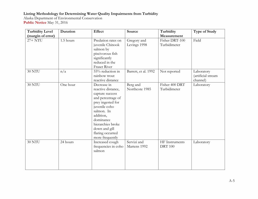
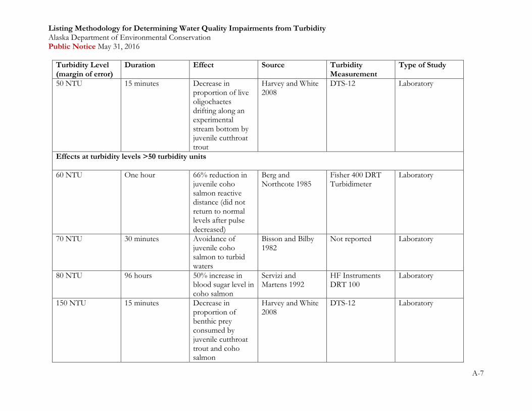
Appendix A provides a summary of effects of increased turbidity at various durations of exposure to
elevated turbidity. Some effects of turbidity on aquatic life can occur at durations as short as one
hour or less. Other direct adverse effects on fish are reported when elevated turbidity levels last two
to three weeks (ODEQ 2014).

Listing Methodology for Determining Water Quality Impairments from Turbidity Alaska Department of Environmental Conservation Public Notice May 31, 2016
3
2 Parameter-Specific Criteria
The turbidity criteria are specified in WQS in 18 AAC 70.020(b)(12) and (24). The turbidity criteria
are as follows:
Table 2.1. Turbidity criteria for fresh water uses
(12) TURBIDITY, FOR
FRESH WATER USES
(criteria are not applicable to
groundwater)
(A) Water Supply
(i) drinking, culinary, and
food processing
May not exceed 5 nephelometric turbidity units (NTU) above
natural conditions when the natural turbidity is 50 NTU or
less, and may not have more than 10% increase in turbidity
when the natural turbidity is more than 50 NTU, not to
exceed a maximum increase of 25 NTU.
(A) Water Supply
(ii) agriculture, including
irrigation and stock
watering
May not cause detrimental effects on indicated use.
(A) Water Supply
(iii) aquaculture
May not exceed 25 NTU above natural conditions. For all
lake waters, may not exceed 5 NTU above natural
conditions.
(A) Water Supply
(iv) industrial
May not cause detrimental effects on established water
supply treatment levels.
(B) Water Recreation
(i) contact recreation
May not exceed 5 NTU above natural conditions when the
natural turbidity is 50 NTU or less, and may not have more
than 10% increase in turbidity when the natural turbidity is
more than 50 NTU, not to exceed a maximum increase of 15
NTU. May not exceed 5 NTU above natural turbidity for all
lake waters.
(B) Water Recreation
(ii) secondary recreation
May not exceed 10 NTU above natural conditions when
natural turbidity is 50 NTU or less, and may not have more
than 20% increase in turbidity when the natural turbidity is
greater than 50 NTU, not to exceed a maximum increase of
15 NTU. For all lake waters, turbidity may not exceed 5
NTU above natural turbidity.
(C) Growth and Propagation of
Fish, Shellfish, Other Aquatic
Life, and Wildlife
Same as (12)(A)(iii).

Listing Methodology for Determining Water Quality Impairments from Turbidity Alaska Department of Environmental Conservation Public Notice May 31, 2016
4
Table 2.2. Turbidity criteria for marine water uses
(24) TURBIDITY, FOR
MARINE WATER USES
(A) Water Supply
(i) aquaculture
May not exceed 25 nephelometric turbidity units (NTU).
(A) Water Supply
(ii) seafood processing
May not interfere with disinfection.
(A) Water Supply
(iii) industrial
May not cause detrimental effects on established levels of
water supply treatment.
(B) Water Recreation
(i) contact recreation
Same as (24)(A)(i).
(B) Water Recreation
(ii) secondary recreation
Same as (24)(A)(i).
(C) Growth and Propagation of
Fish, Shellfish, Other Aquatic Life,
and Wildlife
May not reduce the depth of the compensation point for
photosynthetic activity by more than 10%. May not
reduce the maximum secchi disk depth by more than
10%.
(D) Harvesting for Consumption
of Raw Mollusks or Other Raw
Aquatic Life
Same as (24)(C).
Establishing Natural Conditions for Fresh Water Uses
The term “above natural conditions” is included in the criteria narrative for five of the seven fresh
water uses protected from turbidity. Turbidity data should not be considered in any fresh water
impairment determination without an established natural conditions evaluation for comparison. The
most recent guidance and tools in determining the natural conditions should be used (DEC 2006).
The Quality Assurance Project Plan (QAPP)/Sampling Plan should describe the criteria used to
select the natural conditions site including factors such as flow time between natural and impacted
sites, influence of tributaries in the waterbody segment assessed, and rationale for monitoring
approach (continuous versus grab sampling).
Alaska recognizes that variability in turbidity—among sites and over time—complicates the task of
determining a natural conditions level. Many of Alaska’s waters have naturally occurring turbid
flows, especially glacially fed or tidally influenced waters, and care must be taken to effectively

Listing Methodology for Determining Water Quality Impairments from Turbidity Alaska Department of Environmental Conservation Public Notice May 31, 2016
5
characterize the natural conditions in a scientifically defensible way to establish numeric turbidity
criteria.
Sampling approaches to characterize natural conditions include:
Upstream/downstream: Paired data measurements are taken concurrently in the water at
upstream (natural conditions) and downstream (impacted from a particular pollutant
source) sites. The upstream site to establish the natural conditions should be above any
anthropogenic point or nonpoint sources of turbidity and should have similar stream
geomorphology. Concurrent comparisons of values (natural conditions and impacted
sites) may be difficult especially when grab samples are used. Samples from the natural
conditions site and impacted sites may be collected several hours apart, but should occur
within a reasonable period of time, e.g. no more than one day of flow time between
upstream and downstream sites to be considered concurrent. This is the preferred
approach.
Paired watershed: a nearby water with similar hydrology, morphology, topography, and
other characteristics to the impacted water is identified for use in establishing the natural
conditions. The watershed used to establish the natural conditions should be free of any
anthropogenic point or nonpoint sources of turbidity (EPA 1993, Hughes et al. 1986).
Historic versus current condition: Historic data collected pre-impact is compared to
more recent data collected post-impact in a water.
Magnitude
Magnitude is the numeric threshold for establishing impairment. The criteria component of Alaska’s
WQS sets the magnitude threshold. For turbidity, the criteria are set as a numeric threshold above
the established natural conditions level. In Alaska, the most stringent criterion of the designated
uses applies. For example, the most stringent fresh water criterion protects the contact recreation
use, for which turbidity “may not exceed 5 NTU above natural conditions when the natural
turbidity is 50 NTU or less, and may not have more than 10% increase in turbidity when the natural
turbidity is more than 50 NTU, not to exceed a maximum increase of 15 NTU, and may not exceed
5 NTU above natural turbidity for all lake waters.” The magnitude for most waters has natural
turbidity below 50 NTU, such that the most stringent criterion is usually 5 NTU above natural
conditions (NTU0+5) (Table 2.1).
This methodology is written with the assumption that the critical magnitude threshold for
impairment is 5 NTUs above natural conditions. For particular waters, where this is not the
applicable criterion (e.g. marine waters, glacial rivers and streams with natural conditions above 50
NTUs, waters with site specific criteria or modified uses) then the magnitude threshold and
significance testing procedures should be adjusted to reflect the most stringent applicable criterion.
The designated use for growth and propagation of fish, shellfish, other aquatic life and wildlife is
protected by a criterion allowing turbidity up to 25 NTU above the natural conditions. However,
turbidity has a variety of effects on aquatic life at levels as low as 1-5 NTU above background

Listing Methodology for Determining Water Quality Impairments from Turbidity Alaska Department of Environmental Conservation Public Notice May 31, 2016
6
(ODEQ 2015 and Appendix A). As a result, for clear water rivers and streams where the median
turbidity of the natural condition site is less than 5 NTU, water quality may be considered threatened
and subsequently placed on the CWA §303(d) list for the designated use of growth and propagation
of fish at turbidity levels lower than 25 NTUs above background. In such cases, the water will
already be considered impaired for other uses (e.g. recreation) with more stringent criteria set at 5
NTU over natural background. Adding a threatened status for the growth and propagation use
simply ensures that fish habitat concerns are also addressed.
Duration
In the context of water quality criteria, duration is the period of time (averaging period) over which
ambient water quality data is averaged for comparison with the magnitude threshold (most stringent
criterion). For the purposes of assessing impairment or attainment, a 24-hour daily average is
recommended to evaluate the duration of a turbidity exceedance.
Continuous data collection is preferred with one or more samples collected per hour. Collecting
multiple samples during each day provides more precision in characterizing the 24-hour average,
which makes it easier to distinguish between natural and impacted conditions. Continuous data also
allows evaluations of diurnal or other patterns that may be useful in evaluating potential pollutant
sources and restoration strategies.
However, replicate grab samples taken at the same time during one day are also considered as
representative of the 24-hour averaging period. Even a very small set of samples during each day
may be sufficient to indicate impairment as long as the samples are part of a larger dataset (i.e., at
least 20 days of sampling). A determination of whether a single grab sample can reasonably be
construed to be representative of (i.e., close in value to) average conditions over a specified period is
an important step in the assessment process. The fact that only one grab sample is available for a
particular period (and may not be truly representative of average conditions over the 24-hour period)
does not necessarily mean that it could not be used as the basis of an impairment determination. For
instance, despite being non-representative of the average concentration, it may be indicative of the
average, or at least a fairly reliable indicator of whether or not the average concentration in the
waterbody over a 24-hour period is above or below the level specified in the water quality criterion
(USEPA 2005).
Frequency
The frequency component describes how often an exceedance occurs. Data sets should be evaluated
using the frequency threshold of exceedance during more than 10% of the days sampled to
determine whether a waterbody is considered impaired and listed under CWA §303(d). The U.S.
Environmental Protection Agency (EPA) Consolidated Assessment and Listing Methodology (CALM)
recommends that for conventional pollutants, whenever more than 10% of the water quality
samples collected exceed the criterion threshold, WQS are not attained (USEPA 2002). Turbidity is
a conventional pollutant, so the 10% frequency threshold has been incorporated into this listing
methodology.

Listing Methodology for Determining Water Quality Impairments from Turbidity Alaska Department of Environmental Conservation Public Notice May 31, 2016
7
Impairment Threshold Criteria Statement
The 24-hour daily average (duration)
may not exceed 5 NTU above natural conditions (magnitude)
during more than 10% of the days sampled (frequency).

Listing Methodology for Determining Water Quality Impairments from Turbidity Alaska Department of Environmental Conservation Public Notice May 31, 2016
8
3 Implementing Methods
Data Requirements
Turbidity data should be collected using in-water instruments that measure turbidity in
nephelometric turbidity units (NTU) and meet EPA method 180.1 requirements (USEPA 1983).
The assessment period over which data is collected should span a minimum of two years. The years
do not need to be consecutive, but should be within five years, if possible. During each year of data
collection, samples should be collected over a minimum three-week annual period of concern, to
ensure isolated impacts or weather events do not skew the dataset. The annual period of concern
can range from three weeks to the entire year depending on the characteristics of the pollutants
source(s). A minimum of 20 days sampled at both the natural conditions and impacted sites should
be collected over the assessment period. A minimum of 20 samples was chosen as a balance
between the expense of data collection and the need for sufficient statistical power. Larger data sets
are desirable. The binomial test (See Section 4.2.1) provides statistical confidence in the impairment
or attainment decision.
A “sample” refers to the 24-hour average, as described in section 2.3, which may be calculated from
one or more data points taken during the sampling “day”. Thus, samples should be collected at each
site on a minimum of 20 days over the assessment period.
If using single daily grab samples, DEC recommends collecting more than the minimum number of
samples to increase statistical power of analyses. The preferred method for detecting potential
turbidity impairments is to employ continuous sampling data loggers, which are capable of recording
large data sets (i.e., sampling is performed on an hourly or 15-minute basis) for use in calculating
more representative 24-hour daily averages.
Current data (less than five years old) are generally used for evaluation of turbidity, although some
documentation of data greater than five years old may be relevant if the characteristics of the
pollutant sources remain similar. Older data are generally given less significance when reviewing
information for an impairment determination.
Data should be collected in accordance with a Quality Assurance Project Plan (QAPP). Elements of a
Tier 2 Water Quality QAPP (http://dec.alaska.gov/water/wqapp/wqapp_index.htm) should be used
to ensure the QAPP contains the necessary requirements. For example, the QAPP should outline
the actions that will be taken to reduce data collection errors (e.g., calibration and verification
requirements, recordkeeping requirements). In addition, the QAPP should describe sampling
methods to ensure documentation of any seasonal variations in turbidity sources and the areal extent
of impact.

Listing Methodology for Determining Water Quality Impairments from Turbidity Alaska Department of Environmental Conservation Public Notice May 31, 2016
9
Table 3.1. Summary of data requirements
Description Minimum Requirement
Data Objectives Site selection criteria Select at least one each: natural conditions site and impacted site
The natural conditions site must be a nearby water with waterbody geomorphology similar to impacted site(s).
The impacted site should be representative of anthropogenic impacts and pollutant sources.
Assessment period
Two years
Annual period of concern
Within each year, samples should be collected over a minimum three week time span.
Minimum sample size Samples must be collected on at least 20 days at both the natural conditions and impacted sites.
Representative data Samples collected must be spatially and temporally representative of the areas and period of concern and the natural conditions.
Data Analysis Magnitude Are there exceedances of the turbidity criteria (i.e., natural conditions + 5 NTU)?
Duration Does the exceedance persist over a 24 hour averaging period?
Frequency Do the exceedances occur on more than 10% of the days sampled?
Visual Turbidity Observations
Although visual observations of elevated turbidity may often be noted and lead to identification of
suspected water quality criteria exceedances, Alaska does not make impairment determinations and
the associated CWA §303(d) listings based solely on visual turbidity observations. To confirm
suspected visual exceedances, the results of in-water nephelometric turbidity unit sampling at an
impacted site are compared to the natural conditions.

Listing Methodology for Determining Water Quality Impairments from Turbidity Alaska Department of Environmental Conservation Public Notice May 31, 2016
10
Supplemental data
In order to determine important characteristics of an impaired water, other types of information
may be collected in addition to turbidity data, such as:
Biological, habitat or geomorphology information (e.g., macroinvertebrates, habitat
assessment, riverbank erosion).
Observance of natural or human activities (e.g., storms, recreation activities, nearby
discharge compliance issues) occurring during sampling.
Flow data highly recommended and preferably collected concurrently with turbidity samples.
Historic flow information is also useful for establishing flow rates and patterns that affect
natural turbidity background levels. Flow information will help establish sediment loading if
a total maximum daily load (TMDL) is prepared.
Total Suspended Solids (TSS) data to provide the basis for a weight based load allocation in
a TMDL.
Settleable Solids data to determine if there are exceedances of water quality criteria for
sediment and to characterize potential impacts to the stream bed.

Listing Methodology for Determining Water Quality Impairments from Turbidity Alaska Department of Environmental Conservation Public Notice May 31, 2016
11
4 Data Analysis
Data Review
A quality assurance/quality control data validation review should be conducted prior to analyzing
the data. The methods described in the QAPP should be used to identify outliers. Outliers, or
results that are numerically distant from other data, are fully scrutinized. In certain documented
instances, outliers may be discounted, for example where fouling of equipment occurred.
Discounted outliers may not be used to meet the minimum data requirements or to determine
impairment, attainment or natural conditions.
Impacts from storm events should not be discounted if they are a part of the normal variation in
turbidity during the period of sampling. Storms of unusual magnitude (e.g., 50 or 100 year events),
may be discounted.
The data should be analyzed to determine if there are significant differences between the impacted
and natural conditions sites. Both large and small datasets should be evaluated to determine the
magnitude, frequency and duration of exceedances.
Data Evaluation
Data evaluation techniques will vary depending on the characteristics of the datasets. The sampling
approach used will drive the appropriate data evaluation. The use of statistical tests (hypothesis tests,
confidence intervals) is allowed in the evaluation, when necessary, e.g. to confirm borderline cases.
The flowchart in Figure 4.2 shows the decision process for selecting the appropriate statistical
hypothesis test for evaluating data sets for impairment. The binomial test is recommended for
concurrent (i.e., temporally paired) datasets such as the upstream/downstream approach.
Application of the Distribution of Differences (DoD) is recommended for datasets where data
collected at the natural conditions and impacted sites are not concurrent or temporally paired, such
as the paired watershed or historic versus current conditions approaches.
Data evaluation steps for listing determinations:
1. Evaluate the raw exceedance/attainment estimate.
a. For impairment, the daily average turbidity at the impacted site exceeds the natural
conditions site by 5 NTU on more than 10% of the days sampled (impairment
threshold criteria statement).
b. Conversely, for attainment decisions, the daily average should be less than 5 NTUs
over natural conditions on 90% or more of the days sampled.
2. Conduct the appropriate statistical test (see sections 4.2.1 and 4.2.2) to evaluate the
significance of the raw exceedance or attainment estimate.
3. Based on the results of the statistical test, make the final impairment or attainment
recommendation.

Listing Methodology for Determining Water Quality Impairments from Turbidity Alaska Department of Environmental Conservation Public Notice May 31, 2016
12
Figure 4.2 Flowchart of data evaluation techniques for different sampling approaches
4.1.1 Binomial statistical significance test
The binomial test is a non-parametric, robust, and well known method for characterizing the
probability of proportions. The two data sets must be dependent, which can be confirmed by
statistical testing, if needed. In the case of turbidity, the binomial test is used to determine if the
turbidity criterion (usually natural conditions plus 5 NTUs) is exceeded in more than 10% of the
samples (critical impairment threshold) or in less than 10% of the samples (critical attainment
threshold). The formula for the binomial probability distribution and applications to impairment
decisions were taken from EPA CALM Guidance (USEPA 2002). Following appropriate pairing of
upstream and downstream samples to meet the test requirement for data dependence, the binomial
test is performed on downstream impacted site data from criteria determined by upstream samples
representing the natural conditions site.
Appendix B. provides a full description of the data evaluation and binomial test procedure.
4.1.2 Distribution of Differences statistical significance test
A distribution of differences (DoD) test is recommended for datasets that are not concurrently
measured, i.e. paired watersheds or historic vs current dataset comparisons. The two datasets are
assumed to be independent of each other in time and/or space.
DoD can be used to describe the range of differences between two variables (Hogg et al. 2012; Ott
and Longnecker 2015). In the case of evaluating the impairment threshold for turbidity, the two
variables are daily average turbidity measurements from two locations (e.g., natural conditions and
impacted sites). Given the allowable exceedance frequency for turbidity criteria is 10%, the location
of interest on the DoD curve is the 90th percentile. On this basis, if the 90th percentile of the
turbidity difference is greater than +5 NTU (magnitude threshold), an impairment may be present.

Listing Methodology for Determining Water Quality Impairments from Turbidity Alaska Department of Environmental Conservation Public Notice May 31, 2016
13
Confidence limits around the 90th percentile (Gibbons 2001; US EPA 2002) of the DoD may be
used to determine if there is more (impairment) or less (attainment) than a +5 NTU difference 10%
of the time with statistical significance. Use of confidence limits about the 90th percentile turbidity
difference is therefore termed the ‘DoD test’.
Appendix C. provides a full description of the data evaluation and DoD test procedures.

Listing Methodology for Determining Water Quality Impairments from Turbidity Alaska Department of Environmental Conservation Public Notice May 31, 2016
14
5 Listing Determination Thresholds
Impairment Determination
Before a final decision to add a waterbody impaired by turbidity to the Section 303(d) list/Category
5 (or Category 4b if other pollution controls are in effect), DEC reviews the data for the basic
concepts employed in any listing, including magnitude, frequency and duration. Implementation
tools such as enforcement and permit limitations, should also be evaluated, as necessary, to help
identify ways to effectively reduce the exceedances in future TMDLs or other pollution controls.
The waterbody will be considered impaired if turbidity conditions meet the impairment thresholds
listed below. The most stringent water quality criterion for turbidity impairment can be summarized
as:
Impairment Threshold Criteria Statement:
The 24-hour daily average (duration)
may not exceed 5 NTU above natural conditions (magnitude)
during more than 10% of the days sampled (frequency).
The impairment determination is based on a dataset that
represents the condition of a waterbody segment (spatially and temporally) during an
assessment period of at least two years,
includes a minimum of 20 days sampled (at both natural conditions and impacted sites),
and
characterizes an annual period of concern of at least 3 weeks.
The years of the assessment do not have to be consecutive, but should be within a reasonably short
timeframe, i.e., within 5 years if possible.
In addition, statistical significance testing and other factors may also be considered to corroborate a
listing determination. Other factors may include, but are not limited to: biological data, flow data,
settable solids measurements and TSS measurements.
Attainment Determination
A waterbody may be evaluated for attainment of the water quality criteria for turbidity and placed in
Categories 1 or 2 of Alaska’s Integrated Water Quality Monitoring and Assessment Report as the
result of the following assessments:
1. Initial assessment of a waterbody in Category 3 (insufficient information) of the biennial
Integrated Report
2. Re-assessment of a waterbody with a TMDL for turbidity
3. Re-assessment of a waterbody listed on Alaska’s CWA §303(d) list

Listing Methodology for Determining Water Quality Impairments from Turbidity Alaska Department of Environmental Conservation Public Notice May 31, 2016
15
In general, waterbody attainment determinations should use the listing determination thresholds that
were used to list the waterbodies. For the purposes of evaluating a waterbody for attainment using a
binomial or DoD test, the test should be designed to determine if the daily average turbidity at
impacted site has exceedances (5 NTU over natural conditions) at frequency of less than 10% of the
days sampled.
For a waterbody with an EPA-approved TMDL that uses TSS as an established surrogate for
turbidity, an attainment determination may also need to determine if the point source discharges and
nonpoint source contributions are meeting the wasteload and/or load allocations established in the
TMDL.
For removal of a waterbody from the CWA §303(d) list, both the level of data to support the
removal determination and the burden of proof are no greater than those used in the initial CWA
§303(d) listing determination. If a waterbody was placed on the CWA §303(d) list for turbidity
impairment based on only visual turbidity observations and best professional judgment (in 2008 or
earlier), then a determination to remove the waterbody from the CWA §303(d) list may be based on
visual turbidity observations and best professional judgment alone.
6 References
DEC. 2012. Water Quality Standards 18 AAC 70, amended as of April 8, 2012. DEC, Juneau,
Alaska.
DEC. 2006. Guidance for the Implementation of Natural Condition-Based Water Quality Standards.
http://dec.alaska.gov/water/wqsar/wqs/NaturalConditions.html
Gibbons, R. 2001. A Statistical Approach for Performing Water Quality Impairment Assessments
under the TMDL Program. In: Proceedings of the TMDL Science Issues Conference - St. Louis,
MO. p. 187-198.
Hogg, R., McKean, J., and Craig, A. Introduction to Mathematical Statistics. 7th Edition. Pearson
Education Ltd., Harlow, Essex. 650 pp.
Hughes, R. M., Larsen, D. P., and Omernik, J. M. 1986. Regional reference sites: a method for
assessing stream potentials. Environ Manage. 10(5):629–635.
Oregon Department of Environmental Quality (ODEQ). 2014. Turbidity Technical Review:
Summary of Sources, Effects, and Issues Related to Revising the Statewide Water Quality Standard
for Turbidity. ODEQ, Portland, Oregon.
Ott, L. and M. Longnecker. 2015. An Introduction to Statistical Methods & Data Analysis. 7th
Edition, Cengage Learning, Boston, MA. 1174 pp.
Tetra Tech. 2015. Statistical Approaches for Analyzing Continuous Monitoring Data in the Context
of 303d Listing. Final Technical Memorandum. Tetra Tech, Owings Mills, Maryland.
USEPA. 1983. Methods for Chemical Analysis of Water and Wastes. EPA 600/4-79-020.

Listing Methodology for Determining Water Quality Impairments from Turbidity Alaska Department of Environmental Conservation Public Notice May 31, 2016
16
USEPA. 1993. Paired Watershed Study Design. 841-F-93-009.
USEPA. 2002. Consolidated Assessment and Listing Methodology: Toward a Compendium of Best
Practices. http://www.epa.gov/waterdata/consolidated-assessment-and-listing-methodology-calm
USEPA. 2005. Guidance for 2006 Assessment, Listing and Reporting Requirements Pursuant to
Sections 303(d), 305(b) and 314 of the Clean Water Act. Office of Wetlands, Oceans and
Watersheds. http://water.epa.gov/lawsregs/lawsguidance/cwa/tmdl/upload/2006irg-report.pdf

Listing Methodology for Determining Water Quality Impairments from Turbidity Alaska Department of Environmental Conservation Public Notice May 31, 2016
A-1
Tables of Effects on Aquatic Life
Table A.1. Summary of effects of turbidity on aquatic life in streams1
Turbidity Level (margin of error)
Duration Effect Source Turbidity Measurement
Type of Study
Effects at reported turbidity levels at ≤10 turbidity units
4-8 NTU n/a (reference site approach)
Decrease in Epeorus species in Umatilla River
Scherr, et al. (2011) LaMotte 2020 Field
4.4 NTU n/a (reference site approach)
85% chance of stream being impacted (EPT index <18)
Paul (unpub.) Various Field
5 NTU none given Modelled decrease in primary productivity in clear Alaska streams by 3-13% (stream depth 0.1 – 0.5 m)
Lloyd, et al. 1987 Hach “Portalab” Field
7 NTU Two months 75% decrease in benthic algal biomass
Davies-Colley, et al. 1992
Hach 2100A Field
7 NTU Two months 70% decrease in macroinvertebrate density
Quinn, et al. 1992 Hach 2100A Field
1 Copied from Oregon Department of Environmental Quality (ODEQ). 2014. Turbidity Technical Review: Summary of Sources, Effects, and Issues Related to Revising the Statewide Water Quality Standard for Turbidity. ODEQ, Portland, Oregon.

Listing Methodology for Determining Water Quality Impairments from Turbidity Alaska Department of Environmental Conservation Public Notice May 31, 2016
A-2
Turbidity Level (margin of error)
Duration Effect Source Turbidity Measurement
Type of Study
7-25 NTU n/a Decrease in macroinvertebrate density and other measures of macroinvertebrate health
Prussian, et al. 1999
9 NTU n/a 20% decrease in PREDATOR score using Oregon data
ODEQ turbidity data
n/a Field
10 NTU 15 minutes 50% decrease in brook trout reactive distance
Sweka and Hartman 2001a
Lamotte 2020 turbidimeter
Laboratory
10 NTU 5 days 20% decrease in brook trout growth
Sweka and Hartman 2001b
Lamotte 2020 turbidimeter
Laboratory
10-60 NTU 4-6 days Decrease in prey consumption by juvenile coho salmon after initial exposure to 60 NTU; also, higher response time and increased number of missed strikes at prey.
Berg 1982 DRT-150 Turbidimeter
Laboratory

Listing Methodology for Determining Water Quality Impairments from Turbidity Alaska Department of Environmental Conservation Public Notice May 31, 2016
A-3
Turbidity Level (margin of error)
Duration Effect Source Turbidity Measurement
Type of Study
Effects at reported turbidity levels from 11-20 turbidity units
11-32 NTU 14 days Reduced weight and length gains in newly emerged coho salmon (raceway channels)
Sigler, et al. 1984 Hach 2100A Turbidimeter
Laboratory
15 NTU n/a 20% reduction in rainbow trout reactive distance
Barrett, et al. 1992 Not reported Laboratory (artificial stream channel)
18 NTU 1-10 minutes Reduced feeding rates of small-medium juvenile Chinook salmon on surface prey
Gregory 1994 Fisher DRT-400 Turbidimeter
Laboratory
20 NTU One hour Reduced prey capture success by juvenile coho salmon
Berg and Northcote 1985
Fisher 400 DRT Turbidimeter
Laboratory
Effects at turbidity levels from 21-30 turbidity units
22 NTU 11 days Reduced weight and length gains in newly emerged coho salmon (oval channels)
Sigler, et al. 1984 Hach 2100A Turbidimeter
Laboratory

Listing Methodology for Determining Water Quality Impairments from Turbidity Alaska Department of Environmental Conservation Public Notice May 31, 2016
A-4
Turbidity Level (margin of error)
Duration Effect Source Turbidity Measurement
Type of Study
23 NTU 1-6 hour daily pulses over 9 and 19 days
Reduced abundance and species richness of benthic macroinvertebrates. In addition, reduced rainbow trout length and weight gain when turbidity pulses lasted 4-5 and 5-6 hours, respectively.
Shaw and Richardson 2001
Not reported (converted from suspended sediment concentrations, but does not report relationship)
Laboratory
23 NTU 12 days Reduced startle response by juvenile Chinook salmon
Gregory 1993 Fisher DRT-400 Turbidimeter
Laboratory
25 NTU none given Modelled decrease in primary productivity in clear Alaska streams by 13-50% (stream depth 0.1 – 0.5 m)
Lloyd, et al. 1987 Based on information using Hach “Portalab”
25 NTU 15 minute Reduced drift prey foraging success
Harvey and White 2008
DTS-12 Laboratory
25-35 NTU 3 months Decrease in whole stream metabolism
Parkhill and Gulliver 2002
Not reported Controlled field (laboratory streams)
Listing Methodology for Determining Water Quality Impairments from Turbidity Alaska Department of Environmental Conservation Public Notice May 31, 2016
A-5
Turbidity Level (margin of error)
Duration Effect Source Turbidity Measurement
Type of Study
27+ NTU 1.5 hours Predation rates on juvenile Chinook salmon by piscivorous fish significantly reduced in the Fraser River
Gregory and Levings 1998
Fisher DRT-100 Turbidimeter
Field
30 NTU n/a 55% reduction in rainbow trout reactive distance
Barrett, et al. 1992 Not reported Laboratory (artificial stream channel)
30 NTU One hour Decrease in reactive distance, capture success and percentage of prey ingested for juvenile coho salmon. In addition, dominance hierarchies broke down and gill flaring occurred more frequently
Berg and Northcote 1985
Fisher 400 DRT Turbidimeter
Laboratory
30 NTU 24 hours Increased cough frequencies in coho salmon
Servizi and Martens 1992
HF Instruments DRT 100
Laboratory

Listing Methodology for Determining Water Quality Impairments from Turbidity Alaska Department of Environmental Conservation Public Notice May 31, 2016
A-6
Turbidity Level (margin of error)
Duration Effect Source Turbidity Measurement
Type of Study
Effects at turbidity levels from 31-50 turbidity units
38 NTU 19 days Decreased weight and length gains of newly emerged steelhead (raceway channel)
Sigler, et al. 1984 Hach 2100A Turbidimeter
Laboratory
42 NTU 96 hours 25% increase in blood sugar levels in coho salmon
Servizi and Martens 1992
HF Instruments DRT 100
Laboratory
45 NTU 19 days Decreased weight and length gains of newly emerged steelhead (oval channel)
Sigler, et al. 1984 Hach 2100A Turbidimeter
Laboratory
50 NTU 5 days 50% decrease in brook trout growth rate
Sweka and Hartman 2001b
Lamotte 2020 Turbidimeter
Laboratory
50 NTU 15 minutes Decrease in proportion of drift prey consumed in juvenile cutthroat trout and coho salmon
Harvey and White 2008
DTS-12 Laboratory
Listing Methodology for Determining Water Quality Impairments from Turbidity Alaska Department of Environmental Conservation Public Notice May 31, 2016
A-7
Turbidity Level (margin of error)
Duration Effect Source Turbidity Measurement
Type of Study
50 NTU 15 minutes Decrease in proportion of live oligochaetes drifting along an experimental stream bottom by juvenile cutthroat trout
Harvey and White 2008
DTS-12 Laboratory
Effects at turbidity levels >50 turbidity units
60 NTU One hour 66% reduction in juvenile coho salmon reactive distance (did not return to normal levels after pulse decreased)
Berg and Northcote 1985
Fisher 400 DRT Turbidimeter
Laboratory
70 NTU
30 minutes Avoidance of juvenile coho salmon to turbid waters
Bisson and Bilby 1982
Not reported Laboratory
80 NTU 96 hours 50% increase in blood sugar level in coho salmon
Servizi and Martens 1992
HF Instruments DRT 100
Laboratory
150 NTU 15 minutes Decrease in proportion of benthic prey consumed by juvenile cutthroat trout and coho salmon
Harvey and White 2008
DTS-12 Laboratory

Listing Methodology for Determining Water Quality Impairments from Turbidity Alaska Department of Environmental Conservation Public Notice May 31, 2016
A-8
Turbidity Level (margin of error)
Duration Effect Source Turbidity Measurement
Type of Study
170 NTU Ten days 50% decrease in productivity and 60% decrease in chlorophyll a concentrations
Van Nieuwenhuyse and LaPerreriere (1986)
Hach Portalab Laboratory

Listing Methodology for Determining Water Quality Impairments from Turbidity Alaska Department of Environmental Conservation Public Notice May 31, 2016
A-9
Table A.2. Summary of effects of turbidity on aquatic life in lakes and reservoirs2
Turbidity Level Duration Effect Source Turbidity
Measurement
Lab or Field
Effects at turbidity levels ≤10 turbidity units
~1.2 NTU chronic 50% decrease in
reactive distance of
bluegill trout to avoid
largemouth bass
Miner and Stein 1996 Not reported Laboratory
1.5 NTU 4 hours Minimum turbidity to
decrease reactive
distance of lake,
rainbow, and
cutthroat trout
Mazur and
Beauchamp 2003
LaMotte 2008 Laboratory
1.65 NTU 1 hour Hansen, et al. (2013) LaMotte 2020e h Laboratory
3.18 NTU
4 hours Decrease in reactive
distance of lake trout
to juvenile rainbow
and cutthroat trout at
optimum light
intensity
Vogel and
Beauchamp 1999
LaMotte 2008 Laboratory
5 NTU n/a 80% reduction in
compensation depth
Lloyd, et al. 1987 HF DRT-150
Turbidimeter
Field
5 NTU 3.5 – 42.6 hours Significant decrease
in consumption of
prey by smallmouth
bass
Carter, et al. 2010 LaMotte 2020 Laboratory
10 NTU 19-49 hour Change in size
selectivity of prey by
largemouth bass
Shoup and Wahl 2009 Cole-Parmer Model
8391–40
Laboratory
2 Copied from Oregon Department of Environmental Quality (ODEQ). 2014. Turbidity Technical Review: Summary of Sources, Effects, and Issues Related to Revising the Statewide Water Quality Standard for Turbidity. ODEQ, Portland, Oregon.

Listing Methodology for Determining Water Quality Impairments from Turbidity Alaska Department of Environmental Conservation Public Notice May 31, 2016
A-10
Turbidity Level Duration Effect Source Turbidity
Measurement
Lab or Field
Effects at turbidity levels from 11-20 turbidity units
17-19 NTU n/a Decrease in reactive
distance of
largemouth bass to
crayfish
Crowl 1989 Not reported (Jackson
turbidimeter)
Laboratory
Effects at turbidity levels from 21-30 turbidity units
25 NTU 2 hours 60-80% decrease in
feeding rates of
Lahontan redside
shiner and cutthroat
trout on daphnia
Vinyard and Yuan
1996
DRT-15 Turbidimeter Laboratory
Effects at turbidity levels from 31-50 turbidity units
30+ NTU n/a Limitation in
compensation of
photosynthetic
efficiency for low-
light conditions
Lloyd, et al. 1987 n/a Field
33 NTU n/a (mean turbidity
over multiple lakes
and years)
Reduction in
chlorophyll a levels in
glacial lakes
Koenings, et al. 1990 DRT-100 Field
40 NTU 42-77 hours Decrease in predation
rate by largemouth
bass
Shoup and Wahl 2009 Cole-Parmer Model
8391–40
Laboratory
Effects at turbidity levels >50 turbidity units
60 NTU 3 minutes Decrease in prey
consumption by
bluegill
Gardner 1981 DRT-100 Laboratory

Listing Methodology for Determining Water Quality Impairments from Turbidity Alaska Department of Environmental Conservation Public Notice May 31, 2016
A-11
Turbidity Level Duration Effect Source Turbidity
Measurement
Lab or Field
70 NTU one hour Decrease in predation
rates by largemouth
bass
Reid, et al. 1999 DRT-15B Laboratory
100 NTU n/a Population level
declines of
centrarchids in a
Louisiana
bottomwood
backwater system
Ewing 1991 Hach DR-EL/1 Field
144 NTU 25 weeks No effect on growth
rate of adult crappie
Spier and Heidinger
2002
Hach DR-2000 Field
160 NTU 3 hours No decrease in
predation rate by
rainbow trout;
however, size
selectivity was
affected
Rowe, et al. 2003 Hach 18910
Turbidimeter
Laboratory
174 NTU 25 weeks No decrease in
growth rates of
juvenile white and
black crappie
Spier and Heidinger
2002
Hach DR-2000 Field

Listing Methodology for Determining Water Quality Impairments from Turbidity Alaska Department of Environmental Conservation Public Notice May 31, 2016
A-12
A.1 References3
Abrahams, M., and M. Kattenfeld. 1997. The role of turbidity as a constraint on predator-prey
interactions in aquatic environments. Behavioral Ecology Sociobiology 40:169-174.
American Society for Testing and Materials International (ASTM). 2007. Standard test method for
determination of turbidity above 1 turbidity unit (TU) in static mode: D 7315-07. West
Conshohocken, PA.
Anderson, C. W., 2005. Turbidity (Version 2.1): U.S. Geological Survey Techniques of Water-
Resources Investigations, book 9, chap. A6., section 6.7.
Arruda, J. A., G. R. Marzolf, and R. T. Faulk. 1983. The role of suspended sediments in the nutrition
on zooplankton in turbid reservoirs. Ecology 64:1225-1235.
Bachmann, R. W., B. L. Jones, D. D. Fox, M. Hoyer, L. A. Bull, and D. E. Canfield, Jr. 1996.
Relations between trophic state indicators and fish in Florida (U.S.A.) lakes. Canadian Journal of
Fisheries and Aquatic Sciences 53: 842-855.
Barrett, J. C., G. Grossman, and J. Rosenfeld. 1992. Turbidity-induced changes in reactive distance of
rainbow trout. Transactions of the American Fisheries Society 121:437-443.
Barter, P. J., and T. Deas. 2003. Comparison of portable nephelometric turbidimeters on natural
waters and effluents. New Zealand Journal of Marine and Freshwater Research 37:485-492.
Batiuk, R. A., P. Bergstrom, M. Kemp, E. Kock, L. Murray, J. C. Stevenson, R. Bartleson, V. Carter,
N. B. Rybicki, J. M. Landwehr, C. Gallegos, L. Karrh, M. Naylor, D. Wilcox, K. A. Moore, S. A.
Ailstock, and M. Teichberg. 2000. Chesapeake Bay submerged aquatic vegetation water quality and
habitat-based requirements and restoration targets: a second technical synthesis. Report CBP/TRS
83/92. U.S. EPA Chesapeake Bay Program, Annapolis, MD.
Berg, L. 1982. The effect of exposure of short-term pulses of suspended sediment on the behavior of
juvenile salmonids. Pages 177–196 in G. F. Hartman, editor. Proceedings of the Carnation Creek
workshop: a ten year review, Februrary 24-26, 1982, Nanaimo, BC.
Berg, L., and T. G. Northcote. 1985. Changes in territorial, gill-flaring, and feeding behavior in
juvenile coho salmon (Oncorhynchus kisutch) following short-term pulses of suspended sediment.
Canadian Journal of Fisheries and Aquatic Science 42:1410-1417.
Beschta, R. L. 1980. Turbidity and suspended sediment relationships. Pages 271-282 in Proceedings of
the Watershed Management Symposium, Irrigation and Drainage Division, American Society of Civil
Engineers, Boise, ID, July 21-23, 1980.
3 Copied from Oregon Department of Environmental Quality (ODEQ). 2014. Turbidity Technical Review: Summary of Sources, Effects, and Issues Related to Revising the Statewide Water Quality Standard for Turbidity. ODEQ, Portland, Oregon.

Listing Methodology for Determining Water Quality Impairments from Turbidity Alaska Department of Environmental Conservation Public Notice May 31, 2016
A-13
Beschta, R. L., S. J. O’Leary, R. E. Edwards, and K. D. Knoop. 1981. Sediment and organic matter
transport in Oregon Coast Range streams. WRRI-70. Water Resources Research Institute. Oregon
State University, Corvallis, OR.
Bisson, P. A., and R. E. Bilby. 1982. Avoidance of suspended sediments by juvenile coho salmon.
North American Journal of Fisheries Management 2:371-374.
Boehlert, G. W., and J. B. Morgan. 1985. Turbidity enhances feeding abilities of larval Pacific herring,
Clupea harengus pallasi. Hydrobiologia 123:161-170.
Boese, B. L., B. D. Robbins, and G. Thursby. 2005. Desiccation is a limiting factor for eelgrass
(Zostera marina L.) distribution in the intertidal zone of northeastern Pacific (USA) estuary. Botanica
Marina 48:275-283.
Boese, B. L., W. G. Nelson, C. A. Brown, R. J. Ozretich, H. Lee II, P. J. Clinton, C. L. Folger, T. C.
Mochon-Collura, and T. H. DeWitt. 2009. Lower depth limit of Zostera marina in seven target
estuaries. Pages 219-241 in Lee II, H. and Brown, C.A. (eds.) 2009. Classification of Regional Patterns
of Environmental Drivers And Benthic Habitats in Pacific Northwest Estuaries. U.S. EPA, Office of
Research and Development, National Health and Environmental Effects Research Laboratory,
Western Ecology Division. EPA/600/R-09/140.
Bogen, J., 1980, The hysteresis effect of sediment transport (river) systems: Norsk Geografisk
Tidsskrift. 34:45-54.
Brown, C. A., W. G. Nelson, B. L. Boese, T. H. DeWitt, P. M. Eldridge, J. E. Kaldy, H. Lee II, J. H.
Power, and D. R. Young. 2007. An approach to developing nutrient criteria for Pacific Northwest
estuaries: a case study of Yaquina Estuary, Oregon. USEPA Office of Research and Development,
National Health and Environmental Effects Laboratory, Western Ecology Division. EPA/600/R-
07/046.
Buck, D. H. 1956. Effects of turbidity on fish and fishing. Pages 249-261 in Proceedings of the 21st
North American Wildlife Conference, New Orleans, LA, March 5-7, 1956.
Callaway, R. J., D. T. Specht, and G. R. Dittsoworth. 1988. Manganese and suspended matter in the
Yaquina Estuary, Oregon. Estuaries 11:217-225.
Campbell, D. E. and R. W. Spinrad. 1987. The relationship between light attenuation and particle
characteristics in a turbid estuary. Estuarine, Coastal, and Shelf Science 25:53-65.
Carter, M. W., D. E. Shoup, J. M. Dettmers, and D. H. Wahl. 2010. Effects of turbidity and cover on
prey selectivity of adult smallmouth bass. Transaction of the American Fisheries Society 139:353-361.
Clesceri, L. S., A. E. Greenberg, and A. D. Eaton (eds.) 1994. Standard Methods for the Examination
of Water and Wastewater, 20 ed. American Public Health Association, Washington, DC.
Cline, L. D., R. A. Short, and J. V. Ward. 1982. The influence of highway construction on the
macroinvertebrates and epilithic algae of a high mountain stream. Hydrobiologia 96:149-159.

Listing Methodology for Determining Water Quality Impairments from Turbidity Alaska Department of Environmental Conservation Public Notice May 31, 2016
A-14
Cloern, J. E. 1987. Turbidity as a control on phytoplankton in estuaries. Continental Shelf Research,
7:1367-1381.
Crowl, T. A. 1989. Effects of crayfish size, orientation, and movement on the reactive distance of
largemouth bass foraging in clear and turbid water. Hydrobiologia 183:133-140.
Culp, J. M., F. J. Wrona, and R. W. Davis. 1986. Response of stream benthos and drift to fine
sediment deposition versus transport. Canadian Journal of Zoology 64:1345-1351.
Cyrus, D. P. and S. J. M. Blaber. 1987. The influence of turbidity on juvenile marine fishes in
estuaries: Part 1. Field studies at Lake St. Lucia on the southeastern coast of Africa. Journal of
Experimental Marine Biology and Ecology 109:53-70.
Davies-Colley, R. J., C. W. Hickey, J. M. Quinn, and P. A. Ryan. 1992. Effects of clay discharges on
streams: 1. Optical properties and epilithon. Hydrobiologia 248:215-234.
Davies-Colley, R. J., and D. G. Smith. 2001. Turbidity, suspended sediment, and water clarity: a
review. Journal of the American Water Resources Association 37:1085-1101.
Dearmont, D., B. A. McCarl, and D. A. Tolman. 1998. Cost of water treatment due to diminished
water quality: a case study in Texas. Water Resources Research 34:849–855.
Drake, Doug. 2004. Selecting reference condition sites. An approach for biological criteria and
watershed assessment. ODEQ Technical Report WAS04-002. Oregon Department of
Environmental Quality, Portland, OR.
Drenner, R. W., K. L. Gallo, C. M. Edwards, K. E. Rieger, and E. D. Dibble. 1997. Common carp
affect turbidity and angler catch rates of largemouth bass in ponds. North American Journal of
Fisheries Management 17:1010-1013.
Duarte, C.M. 1991. Seagrass depth limits. Aquatic Botany 40:363-377.
Duchrow, R. M., and W. H. Everhart. 1971. Turbidity measurement. Transactions of the American
Fisheries Society 100:682-690.
Everest, F. H., R. L. Beschta, J. C. Scrivener, K. V. Koski, J. R. Sedell, and C. J. Cedeholdm. 1987.
Fine sediment and salmonid production: a paradox. Pages 98-142 in E.O. Salo and T.W. Cundy,
editors. Streamside management: forestry and fishery interactions 57:98-142.
Ewing, M. S. 1991. Turbidity control and fisheries enhancement in a bottomland hardwood backwater
system in Louisiana (U.S.A.) Regulated Rivers: Research & Management 6:87-99.
Fiksen, O., and J. Giske. 1995. Vertical distribution and population dynamics of copepods by
dynamic optimization. ICES Journal of Marine Science 52:483-503.
Foca, C. 2002. Shedding Light on Treatment Costs: Turbidity's Effect on Potable Water Treatment.
Prepared for degree in Master of Public Administration, University of North Carolina at Chapel Hill.
Ford, J., and C. E. Rose. 2000. Characterizing small subbasins: a case study from coastal Oregon.
Environmental Monitoring and Assessment 64:359–377.

Listing Methodology for Determining Water Quality Impairments from Turbidity Alaska Department of Environmental Conservation Public Notice May 31, 2016
A-15
Forster, D. L., C. P. Bardos, and D.D. Southgate. 1987. Soil erosion and water treatment costs.
Journal of Soil and Water Conservation 42:349-352.
Gadomski, D. M., and M. J. Parsley. 2005. Effects of turbidity, light level, and cover on predation of
white sturgeon larvae by prickly sculpins. Transactions of the American Fisheries Society. 134:369-
374.
Gardner, M. B. 1981. Effects of turbidity on feeding rates and selectivity of bluegills. Transactions of
the American Fisheries Society. 110:446-450.
Giesen, W. B. J. T., M. M. van Katwijk, and C. den Hartog. 1990. Eelgrass condition and turbidity in
the Dutch Wadden Sea. Aquatic Botany 37:71-85.
Gippel, C. J., W. J. Riger, and L. J. Olive. 1991. The effect of particle size and water color on
turbidity. Pages 637-638 in Proceedings of the International Hydrology and Water Resources
Symposium. Perth Australia, October 12-16, 1991.
Gippel, C. J. 1995. Potential of turbidity monitoring for measuring the transport of suspended solids
in streams. Hydrological Processes 9:83-97.
Goldsborough W. J. and W. M. Kemp. 1988. Light responses of a submersed macrophyte:
implications for survival in turbid tidal waters. Ecology 69:1775-1786.
Gradall, K. S., and W. A. Swenson. 1982. Responses of brook trout and creek chubs to turbidity.
Transactions of the American Fisheries Society 111:392-395.
Gregory, R. S. 1990. Effects of turbidity on benthic foraging and predation risk in juvenile Chinook
salmon. Pages 65-73 in C. A. Simenstad, C.A., editor. Proceedings of the Workshop on Effects of
Dredging on Anadromous Pacific Coast Fishes, September 8-9, 1988, Seattle, WA.
Gregory, R. S., and T. G. Northcote. 1993. Surface, planktonic, and benthic foraging by juvenile
Chinook salmon in turbid laboratory conditions. Canadian Journal of Fisheries and Aquatic Science
50:233-240.
Gregory, R. S. 1993. Effect of turbidity on the predator avoidance behavior of juvenile Chinook
salmon. Canadian Journal of Fisheries and Aquatic Science 50: 241-246.
Gregory, R. S. 1994. The influence of ontogeny, perceived risk of predation and visual ability on the
foraging behavior of juvenile Chinook salmon. Pages 271-284 in D. J. Stouder, K. L. Fresh, and R. J.
Feller, editors. Theory and application in fish feeding ecology. Belle Baruch Library of Marine Science
No. 18, University of South Carolina Press, Columbia, SC.
Gregory, R. S., and C. D. Levings. 1996. The effects of turbidity and vegetation on the risk of juvenile
salmonids, Oncorhynchus sp., to predation by adult cutthroat trout, O. clarkii. Environmental Biology
of Fishes 47:279–288.
Gregory, R. S., and C. D. Levings. 1998. Turbidity reduces predation on migrating juvenile Pacific
salmon. Transactions of the American Fisheries Society 127:275-285.

Listing Methodology for Determining Water Quality Impairments from Turbidity Alaska Department of Environmental Conservation Public Notice May 31, 2016
A-16
Gregory, R. S., and T. G. Northcote. 1993. Surface, planktonic, and benthic foraging by juvenile
Chinook salmon in turbid laboratory conditions. Canadian Journal of Fisheries and Aquatic Science
50:233-240.
Grizzel, J. D., and R. L. Beschta. 1993. Municipal water source turbidities following timber harvest
and road construction in Western Oregon: a summary report. Oregon State University, Corvallis,
OR.
Hansen, A. G., D. A. Beauchamp, and E. R. Schoen. 2013. Visual prey detection responses of
piscivorous trout and salmon: Effects of light, turbidity, and prey size. Transactions of the American
Fisheries Society 142(3):854-867.
Harvey, B. C. 1986. Effects of suction gold dredging on fish and invertebrates in two California
streams. North American Journal of Fisheries Management 6:401-409.
Harvey, B. C., and T.E. Lisle. 1998. Effects of suction dredging on streams: a review and evaluation
strategy. Fisheries 23:8-17.
Harvey, B. C., and S. F. Railsback. 2009. Exploring the persistence of stream-dwelling trout
populations under alternative real-world turbidity regimes with an individual-based model.
Transactions of the American Fisheries Society 138:348-360.
Harvey, B. C., and S. F. Railsback. 2004. Elevated turbidity reduces abundance and biomass of stream
trout in an individual-based model. Draft manuscript. Redwood Sciences Laboratory, U. S.
Department of Agriculture Forest Service, Arcata, CA.
Harvey, B. C., and J. L. White. 2008. Use of benthic prey by salmonids under turbid conditions in a
laboratory stream. Transactions of the American Fisheries Society 137:1756-1763.
Holmes, T. P. 1988. The offsite impact of soil erosion on the water treatment industry. Land
Economics 64:356-366.
Holmes, T. P. 1988. The offsite impact of soil erosion on the water treatment industry. Land
Economics 64:356-366.
Huber, C., and D. Blanchet. 1992. Water Quality Cumulative Effects of Placer Mining on the
Chugach National Forest, Kenai Peninsula, 1988-1990. Chugach National Forest, Anchorage.
Hubler, S. 2007a. Development and use of RIVPACS-type macroinvertebrate models to assess the
biotic integrity of wadeable Oregon streams: PREDATOR. DEQ06-LAB-0062-TR. Oregon
Department of Environmental Quality, Watershed Assessment Section. Portland, OR.
Hubler, S. 2007b. Wadeable stream conditions in Oregon. DEQ07-LAB-0081-TR. Oregon
Department of Environmental Quality, Watershed Assessment Section. Portland, OR.
Hughes, R.M., S. Howlin, and P.R. Kaufmann. 2004. A Biointegrity Index for Coldwater Streams of
Western Oregon and Washington. Transactions of the American Fisheries Society 133:1497-1515.

Listing Methodology for Determining Water Quality Impairments from Turbidity Alaska Department of Environmental Conservation Public Notice May 31, 2016
A-17
Hughes, R. M., and J. R. Gammon. 1987. Longitudinal changes in fish assemblages and water quality
in the Willamette River, Oregon. Transactions of the American Fisheries Society 116:196–209.
Independent Multidisciplinary Science Team (IMST). 2006. IMST review of Oregon Department of
Environmental Quality’s Technical basis for revising turbidity criteria (DEQ Water Quality Division,
October 2005 Draft).
Johnson, M. L., G. Pasternack, J. Florsheim, I. Werner, T. B. Smith, L. Bowen, M. Turner, J. Viers, J.
Steinmetz, J. Constantine, E. Huber, O. Jorda, and J. Feliciano. 2002. North Coast River loading
study: Road crossing on small streams. Volume 2. Stressors of salmonids. Report CTSW-RT-02-040.
Prepared for the Division of Environmental Analysis, California Department of Transportation,
Sacramento, CA.
Kirk, J. T. O. 1985. Effects of suspensoids (turbidity) on penetration of solar radiation in aquatic
ecosystems. Hydrobiologia 125:195-208.
Koenings, J. P., R. D. Burkett, and J. M. Edmundson. 1990. The exclusion of limnetic cladocera from
turbid glacier-meltwater lakes. Ecology 71:57-67.
Landers, M. N. 2002. Summary of blind sediment reference sample measurement session. In J. R.
Gray and G. D. Glysson, editors. Proceedings of the Federal Interagency Workshop on Turbidity and
other Sediment Surrogates. April 30-May 2, 2002, Reno, Nevada.
Lara-Lara, J. R., B. E. Frey, and L. F. Small. 1990. Primary production in the Columbia River Estuary.
I. Spatial and temporal variability of properties. Pacific Science 44:17-37.
LaSalle, M. W. 1990. Physical and chemical alterations associated with dredging. Pages 1-12 in C. A.
Simenstad (ed.) Proceedings, Workshop on the effects of dredging on anadromous Pacific Coast
fishes. Washington Sea Grant Program, Seattle.
Lewis, J., R. Eads, and R. Klein. 2007. Comparisons of Turbidity Data Collected with Different
Instruments. Report on a Cooperative Agreement between the California Department of Forestry
and Fire Protection and USDA Forest Service -- Pacific Southwest Research Station (PSW Agreement
#06-CO-11272133-041).
Ljunggren, L., and A. Sandström. 2007. Influence of visual conditions on foraging and growth of
juvenile fishes with dissimilar sensory physiology. Journal of Fish Biology 70:1319-1334.
Lloyd, D. B., J. P. Koenings, and J. D. LaPerriere. 1987. Effects of turbidity in fresh waters of Alaska.
North American Journal of Fisheries Management 7:18–33.
May, C. L., and D. C. Lee. 2004. The relationships among in-channel sediment storage, pool depth,
and summer survival of juvenile salmonids in Oregon Coast Range streams. North American Journal
of Fisheries Management 24:761-774.
Mazur, M. M., and D. A. Beauchamp. 2003. A comparison of visual prey detection among species of
piscivorous salmonids: effects of light and low turbidities. Environmental Biology of Fishes 67:397-
405.

Listing Methodology for Determining Water Quality Impairments from Turbidity Alaska Department of Environmental Conservation Public Notice May 31, 2016
A-18
Mills, K., L. Dent, and J. Robben. 2003. Wet season road use monitoring report. Forest Practices
Monitoring Program Technical Report Number 17. Oregon Department of Forestry, Salem, OR.
Moore, K. A., H. A. Neckles, and R. J. Orth. 1996. Zostera marina (eelgrass) growth and survival
along a gradient of nutrients and turbidity in the lower Chesapeake Bay. Marine Ecology Progress
Series 142:247-259.
Moore, W. B., and B. A. McCarl. 1987. Off-site costs of soil erosion: a case study in the Willamette
Valley. Western Journal of Agricultural Economics 12:42-49.
Morgan, C. A, J. R. Cordell, and C. A. Simenstad. 1997. Sink or swim? Copepod population
maintenance in the Columbia River estuarine turbidity maxima region. Marine Biology 129:309-317.
Morgan, S. R. 1992. Seasonal and tidal influence of the estuarine turbidity maximum on primary
biomass and production in the Columbia River estuary. M.S. thesis, Oregon State Univ., Corvallis,
OR.
Moring, J. R. 1975. The Alsea Watershed Sturdy: effects of logging on the aquatic resources of three
headwater streams of the Alsea River, Oregon. Part II – Changes in environmental conditions.
Fishery Research Report Number 9 (Part 2), Oregon Department of Fish and Wildlife, Corvallis, OR.
Mulvey, M., and A. Hamel. 1998. Winter storm turbidity and biological integrity of Oregon Coast
streams 1997. DEQ Biomonitoring Report 98-005. Laboratory Division Biomonitoring Section,
Oregon DEQ, Portland, OR.
Mulvey, M., R. Leferink, and A. Borisenko. 2009. Willamette Basin Rivers and Streams Assessment.
Report DEQ 09-LAB-016. Laboratory and Environmental Assessment Division, Watershed
Assessment Section, Oregon Department of Environmental Quality, Hillsboro, OR.
National Council for Air and Stream Improvement (NCASI). 2002. Long-term Receiving Water Data
Compendium: August 1998 to September 1999. Technical Bulletin No. 843. Anacortes, WA.
NCASI. 2003a. Long-term Receiving Water Study Data Compendium: September 2000 to August
2001. Technical Bulletin No. 868. Anacortes, WA.
NCASI. 2003b. Long-term Receiving Water Study Data Compendium: September 1999 to August
2000. Technical Bulletin No. 856. Anacortes, WA.
National Drinking Water Clearinghouse. 1996. Tech Brief: Filtration.
http://www.nesc.wvu.edu/pdf/dw/publications/ontap/2009_tb/filtration_DWFSOM51.pdf
Natural Resources Conservation Service (NRCS). 2007. 2003 Natural Resources Inventory.
Washington, DC.
Naymik, J., Y. Pan, and J. Ford. 2005. Diatom assemblages as indicators of timber harvest effects in
coastal Oregon streams. Journal of the North American Benthological Society 24:569–584.
Newcombe, C. P. 2003. Impact assessment model for clear water fishes exposed to excessively cloudy
water. Journal of the American Water Resources Association 39:529–544.

Listing Methodology for Determining Water Quality Impairments from Turbidity Alaska Department of Environmental Conservation Public Notice May 31, 2016
A-19
Odum, E. P. 1985. Trends Expected in Stressed Ecosystems. BioScience 35:419-422.
ODEQ. 2008. Rogue River Basin TMDL. Water Quality Division, Oregon Department of
Environmental Quality.
ODEQ. 2010. Turbidity analysis for Oregon public water systems: Water quality in Coast Range
drinking water source areas. DEQ Report 09-WQ-024. Water Quality Division, Oregon Department
of Environmental Quality, Portland, OR.
Parkhill, K. L., and J. S. Gulliver. 2002. Effect of inorganic sediment on whole stream productivity.
Hydrobiologia 472:5-17.
Paul, John. Unpub. Conditional Probability Approach for Identifying Threshold of Impact for
Sedimentation using Turbidity as a Surrogate Measure in Freshwater Streams in
Coast Range Ecoregion in Oregon - Application Using 1994-95 REMAP Data. Unpublished draft
data.
Paustian, S. J. and R. L. Beschta. 1979. The suspended sediment regime of an Oregon Coast Range
stream. Water Resources Bulletin 15:144–154.
Preisendorfer, R. W. 1986. Secchi disk science: Visual optics of natural waters. Limnology and
Oceanography 31:909-926.
Prussian, A.M, T.V. Royer, and G.W. Minshall. 1999. Impact of suction dredging on water quality,
benthic habitat, and biota in the Fortymile River, Resurrection Creek, and Chatanika River, Alaska.
Final report prepared for USEPA Region 10, Seattle, WA.
Quesenberry NJ, Allen PJ, Cech JJ. The influence of turbidity on three-spined stickleback foraging.
Journal of Fish Biology 70(3), 965-972. 2007.
Quinn, J. M., R. J. Davies-Colley, C. W. Hickey, M. L. Vickers, and P. A. Ryan. 1992. Effects of clay
discharges on streams: 2. Benthic invertebrates. Hydrobiologia 248:235-247.
Reid S. M., M. G. Fox, and T. H. Whillans. 1999. Influence of turbidity on piscivory in largemouth
bass (Micropterus salmoides). Canadian Journal of Fisheries and Aquatic Science 56:1362–1369.
Reiter, M., J. T. Heffner, S. Beech, T. Turner, and R. E. Bilby. 2009. Temporal and spatial turbidity
patterns over 30 years in a managed forest of western Washington. Journal of the American Water
Resources Association 45:793-808.
Reynolds, J. B., R. C. Simmons, and A. R. Burkholder. 1989. Effects of placer mining discharge on
health and food of the Arctic grayling. Water Resources Bulletin 25:625-635
Risley, J. C., and A. Laenen. 1999. Upper Klamath Lake Basin Nutrient-Loading Study— Assessment
of Historic Flows in the Williamson and Sprague Rivers. U. S. Geological Survey Scientific
Investigations Report 98-4198. Prepared in cooperation with the U.S. Bureau of Reclamation.
Portland, OR.

Listing Methodology for Determining Water Quality Impairments from Turbidity Alaska Department of Environmental Conservation Public Notice May 31, 2016
A-20
Rowe, D. K., T. L. Dean, E. Williams, and J. P. Smith. 2003. Effects of turbidity on the ability of
juvenile rainbow trout, Oncorhynchus mykiss, to feed on limnetic and benthic prey in laboratory
tanks. New Zealand Journal of Marine and Freshwater Research. 37:45-52.
Sadar, M. J. 1996. Turbidity science. Technical Information Series Booklet No. 11. HACH Technical
Center for Applied Analytical Chemistry, Loveland, CO.
Scannell, P. O. 1988. Effects of elevated sediment levels from placer mining on survival and behavior
of immature Arctic grayling. Master's of Science Thesis. University of Alaska, Fairbanks.
Scherr, M.A., D.E. Wooster, and S. Rao. 2011. Interactions between macroinvertebrate taxa and
complex environmental gradients influencing abundance and distribution in the Umatilla River,
Northeastern Oregon. Journal of Freshwater Ecology 26(2):255-266.
Schwartz, J. S., M. Dahle, and R. B. Robinson. 2008. Concentration-duration-frequency curves for
stream turbidity: possibilities for assessing biological impairment. Journal of the American Water
Resources Association 44:879-886.
Servizi, J. A., and D. W. Martens. 1992. Sublethal responses of coho salmon (Oncorhynchus kisutch)
to suspended sediments. Canadian Journal of Fisheries and Aquatic Science 49:1389-1395.
Shaw, E. A., and J. S. Richardson. 2001. Direct and indirect effects of sediment pulse duration on
stream invertebrate assemblages and rainbow trout (Onchorhynchus mykiss) growth and survival.
Canadian Journal of Fisheries and Aquatic Science 58:2213-2221.
Shoup, D. E., and D. H. Wahl. 2009. The effects of turbidity on prey selection by piscivorous
largemouth bass. Transactions of the American Fisheries Society 138:1018-1027.
Shrader, T. 2000. Effects of sediment loading and associated turbidity on the trophic dynamics of a
central Oregon reservoir. Information Reports Number 2000-02. Oregon Department of Fish and
Wildlife, Portland, OR.
Sigler, J. W., T. C. Bjornn, and F. H. Everest. 1984. Effects of chronic turbidity on density and growth
of steelheads and coho salmon. Transactions of the American Fisheries Society 113:142-150.
Slaney, P. A., T. G. Halsey, and A. F. Tautz. 1977. Effects of forest harvesting practices on spawning
habitat of stream salmonids in the Centennial Creek Watershed, British Columbia. Fisheries
Management Report No. 73. Ministry of Environment, Lands and Parks, Victoria, BC.
Smith, D. G. 2001. A protocol for standardizing Secchi disk measurements, including use of a viewer
box. Lake and Reservoir Management 17:90-96.
Smith, D. G., A. M. Cragg, and G. F. Croker. 1991. Water clarity criteria for bathing waters based on
user perception. Journal of Environmental Management 33:285-299.
Smith, D. G., G. S. Croker, and K. McFarlane, 1995a. Human perception of water appearance: 1.
Clarity and colour for bathing and aesthetics. New Zealand Journal of Marine and Freshwater
Research 29:29-43.

Listing Methodology for Determining Water Quality Impairments from Turbidity Alaska Department of Environmental Conservation Public Notice May 31, 2016
A-21
Smith, D. G., G. S. Croker and K. McFarlane, 1995b. Human perception of water appearance: 2.
Colour judgment and the influence of perceptual set on the perceived water suitability for use. New
Zealand Journal of Marine and Freshwater Research 29:45-50.
Smith, D. G., and R. J. Davies-Colley. 1992. Perception of water clarity and color in terms of
suitability for recreational use. Journal of Environmental Management 36:226-235.
Smith, D. G., R. J. Davies-Colley, J. Knoeff, and G. W. J. Slot. 1997. Optical characteristics of New
Zealand Rivers in relation to flow. Journal of the American Water Resources Association 33:301-312.
Smith, D. G., and J. A. Perrone. 1996. Laboratory experiments to investigate human sensitivity to
changes in water clarity. Journal of Environmental Management 48:139-154.
Sorensen, D. L., M. M. McCarthy, E. J. Middlesbrooks, and D. B. Porcella. 1977. Suspended and
dissolved solids effects on freshwater biota: a review. USEPA, Office of Research and Development,
Corvallis, OR.
Stewart, D., and D. Sharp. 2003. A recreational suction dredge mining water quality study on South
Fork Clearwater River, Idaho County, Idaho. Water Quality Summary Report 34. Idaho Department
of Environmental Quality, Boise, ID.
Suren, A.M., M.L. Martin, and B.J. Smith. 2005. Short-term effects of high suspended sediments on
six common New Zealand stream invertebrates. Hydrobiologia 548:67-74.
Sweka, J. A., and K. J. Hartman. 2001a. Influence of turbidity on brook trout reactive distance and
foraging success. Transactions of the American Fisheries Society 130:138-146.
Sweka, J. A. and K. J. Hartman. 2001b. Effects of turbidity on prey consumption and growth in brook
trout and implications for bioenergetics modeling. Canadian Journal of Fisheries and Aquatic Sciences
58:386-393.
Telesnicki, G. J., and W. M. Goldberg. 1995. Comparison of turbidity measurement by nephelometry
and transmissometry and its relevance to water quality standards. Bulletin of Marine Science 57:540-
547.
Thom, R. M., S. L. Southard, A. B. Borde, and P. Stoltz. 2008. Light requirements for growth and
survival of eelgrass (Zostera marina L.) in Pacific Northwest (USA) estuaries. Estuaries and Coasts
31:969-980.
Thomas, V. G. 1985. Experimentally determined impacts of a small, suction gold dredge on a
Montana stream. North American Journal of Fisheries Management 5:480-488.
Uhrich, M. A. and H. M. Bragg. 2003. Monitoring instream turbidity to estimate continuous
suspended-sediment loads and yields and clay-water volumes in the Upper North Santiam River
Basin, Oregon, 1998-2000. Water Resources Investigations Report 03-4098, U.S. Geological Survey,
Reston, VA.
United States Environmental Protection Agency (USEPA). 1976. Quality criteria for water. PB-
263943. Office of Water Planning and Standards, Washington, DC.

Listing Methodology for Determining Water Quality Impairments from Turbidity Alaska Department of Environmental Conservation Public Notice May 31, 2016
A-22
USEPA. 1993. Method 180.1: Determination of turbidity by nephelometry. Revision 2.0.
Environmental Monitoring Systems Laboratory, Cincinnati, OH.
USEPA. 1999. Guidance manual for compliance with the Interim Enhanced Surface Water Treatment
Rule: Turbidity provisions. EPA 815-R-99-010. Office of Water. Washington, DC.
USEPA. 2003. Ambient water quality criteria for dissolved oxygen, water clarity and chlorophyll a for
Chesapeake Bay and tidal tributaries. Chesapeake Bay Program Office, Annapolis, MD.
USEPA. 2006. Framework for developing suspended and bedded sediments (SABS) water quality
criteria. EPA-822-R-06-001. Office of Water and Office of Research and Development, Washington,
DC.
United States General Accounting Office (USGAO). 1998. Oregon watersheds: many activities
contribute to increased turbidity during large storms. GAO/RCED-98-220. Washington, DC.
Utne-Palm, A. C. 2002. Visual feeding of fish in a turbid environment: Physical and behavioral
aspects. Marine and Freshwater Behavior and Physiology. 35:111-128.
Van Nieuwenhuyse, E. E. 1983. The effects of placer mining on the primary productivity of interior
Alaska streams. Master of Science Thesis. University of Alaska Fairbanks.
Van Nieuwenhuyse, E. E., and J. D. LaPerriere. 1986. Effects of placer gold mining on primary
production in subarctic streams of Alaska. Water Resources Bulletin 22:91-99.
Vinyard, G. L., and A.C. Yuan. 1996. Effects of turbidity on feeding rates of Lahontan cutthroat trout
(Oncorhynchus Clarkii Henshawi) and Lahontan redside shiner (Richardsonius egregius). Great Basin
Naturalist 56:157-161.
Vogel, J. L., and D.A. Beauchamp. 1999. Effects of light, prey size, and turbidity on reaction distances
of lake trout (Salvelinus namaycush) to salmonid prey. Canadian Journal of Fisheries and Aquatic
Sciences 56:1293-1297.
Ward, H. B. 1938. Placer mining on the Rogue River, Oregon, in Its relation to the fish and fishing in
that stream. Bulletin No. 10. Prepared for the Oregon State Department of Geology and Mineral
Industries, Portland, OR.
White, J. L., and B. C. Harvey. 2007. Winter feeding success of stream trout under different
streamflow and turbidity conditions. Transactions of the American Fisheries Society 136:1187-1192.
Wilber, D. H. and D. G. Clarke. 2001. Biological effects of suspended sediments: a review of
suspended sediment impacts on fish and shellfish with relation to dredging activities in estuaries.
North American Journal of Fisheries Management. 21:855-875.

Listing Methodology for Determining Water Quality Impairments from Turbidity Alaska Department of Environmental Conservation Public Notice May 31, 2016
A-23
Binomial statistical test
B.1 Binomial raw exceedances
For paired datasets that were collected concurrently, the raw exceedance frequency is calculated by
comparing the 24-hour daily averages of the impacted site dataset to the natural conditions dataset. If
the daily average at the impacted site exceeds the natural conditions site by more than 5 NTU (the
magnitude threshold,) then it is counted as a raw exceedance.
Figure B.1 shows an example time series plot of the daily averages of an impacted site and natural
conditions site. In this example, the impacted site and natural conditions site were monitored
continuously via data loggers that collected 24 hourly samples each day for 84 days. Daily averages
were calculated for each day. In the figure, the most stringent criterion (for water recreation, contact
recreation) is calculated by adding 5 NTU to the 24-hour daily averages at the natural conditions site.
Figure B.1. Time series plot of average daily turbidity for the criterion (natural conditions + 5 NTU) and impacted site. 4
The daily average criterion was exceeded at the impacted site on 63 of 84 days (as shown in Figure
B.1), resulting in a raw exceedance frequency of 75%. Table B.1 shows the exceedance frequencies for
the designated uses of water recreation, contact recreation (natural conditions +5 NTU), water
recreation, secondary recreation (natural conditions +10 NTU) and growth and propagation of fish,
shellfish, other aquatic life and wildlife (natural conditions +25 NTU). In this example, the impacted
site exceeds all criteria for water recreation by a frequency more than 10%. The next step would be to
conduct a statistical test to make an impairment determination.
4 Turbidity was not measured at the impacted site from June 29 through July 20, so these days are not included in the raw frequency.
0.00
10.00
20.00
30.00
40.00
50.00
60.00
Dai
ly A
vera
ge T
urb
idit
y (N
TU) Impacted Site
NTU 0+5

Listing Methodology for Determining Water Quality Impairments from Turbidity Alaska Department of Environmental Conservation Public Notice May 31, 2016
A-24
Table B.1. Example raw exceedance frequency calculation
Water recreation, contact recreation (natural conditions + 5 NTU)
Water recreation, secondary recreation (natural conditions + 10 NTU)
Growth and propagation of fish, shellfish, other aquatic life and wildlife (natural conditions + 25 NTU)
Total exceedances 63 42 5
Total samples (24-hour daily averages)
84 84 84
Raw exceedance frequency
75% 50% 6%
B.2 Binomial statistical significance test
If the raw exceedance frequency exceeds 10% at the downstream or impacted site, then the binomial
test should be conducted. Example inputs, outputs, and decisions of the test are listed in Table B.2.
Additional detail and discussion of the binomial test is provided by US EPA (2002). The calculations
for the binomial test can be done using the ADEC Turbidity Hypothesis Test Template (DEC 2016).
Table B.2. Example binomial test inputs and outputs for secondary recreation listing case
Description Value Comments
Input
Total Exceedances 42 Number of downstream samples greater than criterion
Total Trials 84
Number of comparisons of downstream site to the criterion obtained from upstream data. Equals number of matched pair upstream/downstream samples.
Raw Exceedance Frequency 50% Calculated as Exceedances / Trials
Target Type I Error (α) 0.2
α = 0.2 for trials < 40, α = 0.1 for trials > 40. Alternate values of α considered to balance or improve statistical power of test.
Allowed Exceedance Rate 10% Allowed by US EPA guidance for conventional parameters
Output
Actual Type I Error(αa) 0.1330 Actual Type 1 error calculated from discrete trial and exceedance combinations. Intermediate output.
Minimum Exceedances to Reject
4 Number of exceedances needed to reject null hypothesis at the acceptable Type 1 error level. Intermediate output.
Binomial Test Statistic (P) 0.0000 p-value, or attained significance level, of Binomial Test.
Final Result Impaired?* Yes
If p-value < Target Type 1 error, then reject null hypothesis and conclude waterbody exceeds criterion greater than 10% of the time.

Listing Methodology for Determining Water Quality Impairments from Turbidity Alaska Department of Environmental Conservation Public Notice May 31, 2016
A-25
*For impairment determination:
Null Hypothesis: Exceedance Frequency < 10% (not impaired)
Alternate Hypothesis: Exceedance Frequency > 10% (impaired)
For attainment determination:
Null Hypothesis: Exceedance Frequency > 10% (not attaining)
Alternate Hypothesis: Exceedance Frequency < 10% (attaining)
The binomial P-value (Table B.2) is the test statistic. If the test statistic is less than the Actual Type I
Error rate, then the null hypothesis should be rejected and the water should be considered impaired
(or attaining).
The final result from the binomial test will be used to determine if the turbidity significantly exceeds
or attains the 10% frequency threshold.
B.3 References
DEC. 2016. ADEC Turbidity Hypothesis Tests Template., dated March 31, 2016.
[http://dec.alaska.gov/water/wqsar/waterbody/integratedreport.htm]
USEPA. 2002. Consolidated Assessment and Listing Methodology: Toward a Compendium of Best
Practices. http://www.epa.gov/waterdata/consolidated-assessment-and-listing-methodology-calm

Listing Methodology for Determining Water Quality Impairments from Turbidity Alaska Department of Environmental Conservation Public Notice May 31, 2016
A-26
Distribution of Differences test
A distribution of differences (DoD) test is recommended for datasets of daily average turbidity that
are not concurrently measured, i.e. paired watersheds or historic vs current dataset comparisons. The
DoD test requires random, independent, and normally distributed data. Note that turbidity data
usually must be transformed to achieve a normal distribution. In most instances this is a log
transformation. The calculations for the binomial test can be done using the ADEC Turbidity
Hypothesis Test Template (DEC 2016).
C.1 Distribution of Differences raw percentile inspection
The raw criterion exceedance frequency can be determined from inspection of the cumulative DoD.
The cumulative DoD (see example in Table 4.2.3) is calculated as follows:
1. Transform reference and impacted site datasets to achieve a normal distribution. Unless
otherwise informed, a log transform is assumed.
2. Calculate the mean and standard deviation of the DoD.
The difference [impacted (X) – natural conditions (Y)] between two random, independent and
normally distributed variables (X and Y) is a normal distribution having the following mean
and standard deviation (in log units).
mean difference = µX-Y = µX - µY and standard deviation of difference =
𝜎𝑋 −𝑌 = √𝑠𝑥2
𝑛𝑋+
𝑠𝑌2
𝑛𝑌
where:
µX is the mean of variable X
µY is mean of variable Y
sX sample standard deviation of variable x
sY is sample standard deviation for Y
nX is sample size for variable X
nY is sample size for variable Y
3. Calculate ascending percentiles of the DoD using the inverse function for a normal
distribution to obtain the cumulative DoD. The inverse function is available in several
software packages, including MS Excel as the ‘Norm.Inv’ function.
4. Convert inverse function output from log units to NTU.
Table C.1 shows an example cumulative DoD having a mean difference of 6.7 NTU and standard
deviation difference of 1.9 NTU. Two important observations may be obtained from Table C.1 First,
the magnitude of the 90th percentile (10% exceedance frequency) is greater than +5 NTU suggesting
an impairment may exist. Second, a 5 NTU difference occurs at approximately the 35th percentile.
Since exceedance frequency is calculated as 100 percentile, the latter observation indicates a raw
exceedance frequency of approximately 100 – 35 = 65%.

Listing Methodology for Determining Water Quality Impairments from Turbidity Alaska Department of Environmental Conservation Public Notice May 31, 2016
A-27
Table C.1. Percentiles of the Difference Distribution between Impacted and Natural Conditions Datasets
Difference Percentile Impacted – Natural Conditions (Difference in NTU)
99 31.2
90 15.6
80 11.7
70 9.4
60 7.9
50 6.7
40 5.6
30 4.7
20 3.8
10 2.9
1 1.4
C.2 Distribution of Differences statistical significance test
If inspection of DoD percentiles indicates the impacted site exceeds the criterion at or above the 10%
frequency threshold, i.e. the NTU difference at the 90th percentile is greater than +5, then the DoD
test should be conducted. The DoD test implements the confidence interval approach to listing and
delisting decisions (Gibbons 2001, US EPA 2002). With this approach, a difference of +5 NTU is
compared to confidence limits of the 90th percentile.
For impairment determination purposes, the hypothesis test of interest is a one-sided Lower
Confidence Limit (LCL) on the 90th percentile of the difference distribution. If the LCL is greater
than +5 NTU, then we can infer that the difference between impact and reference is significantly
greater than 5 NTU (i.e. exceeds the magnitude threshold for impairment) at the frequency threshold
of 10%. Figure C.2.1 shows an example distribution where the LCL is greater than +5 NTU, thus
impaired. Figure C.2.2 shows an example distribution where the LCL is less than +5 NTU. In this
case, the waterbody would not be considered impaired.
For attainment determination purposes, the hypothesis test of interest is a one-sided Upper
Confidence Limit (UCL) on the 90th percentile of the difference distribution. If the UCL is less than
+5 NTU, then we can infer that the difference between impacted site and natural conditions site is
significantly less than +5 NTU (attaining) at the frequency threshold of 10%. Figure C.2.3 shows a
distribution where the UCL is greater than +5 NTU. This waterbody would not be attaining WQS
and could not be delisted. Alternately, figure C.2.4 shows a distribution where the UCL is less than +5
NTU. This would lead to an attainment decision and delisting.
A one-sided confidence limit is calculated using a Wald type confidence interval given as:
Confidence Limit (as percentile, CLp) = (0.90 + zα * σπ ) where zα is the z associated with alpha (e.g.,
1.28 for alpha = 0.1) and σπ is the standard error of the proportion difference given by the variance
sum law below:

Listing Methodology for Determining Water Quality Impairments from Turbidity Alaska Department of Environmental Conservation Public Notice May 31, 2016
A-28
𝜎𝜋 = √𝜋𝑋 (1 − 𝜋𝑋)
𝑛𝑋+
𝜋𝑌 (1 − 𝜋𝑌)
𝑛𝑌
Where πX and πY = 0.90 as percentiles of interest and alpha (α) is the Type 1 error rate assumed for
the test.
The one-sided LCL expressed as a percentile (LCLp) is calculated as 0.90 - zα * σπ . Two steps are
required to convert the LCLp into NTUs. First, the LCLp is used as input to the inverse function for
a normal distribution along with µX-Y (log units) and σX-Y (log units). Output from the first step is the
LCL in log NTUs. The second step is to reverse the log transform (e.g., eLCL for natural log
transform). Similarly, for attainment the one-sided UCL expressed as a percentile (UCLp) is calculated
as 0.90 + zα * σπ and converted to NTUs as described above.
Figure C.2.1. Example listing determination – the LCL is greater than +5 NTU = Impaired.
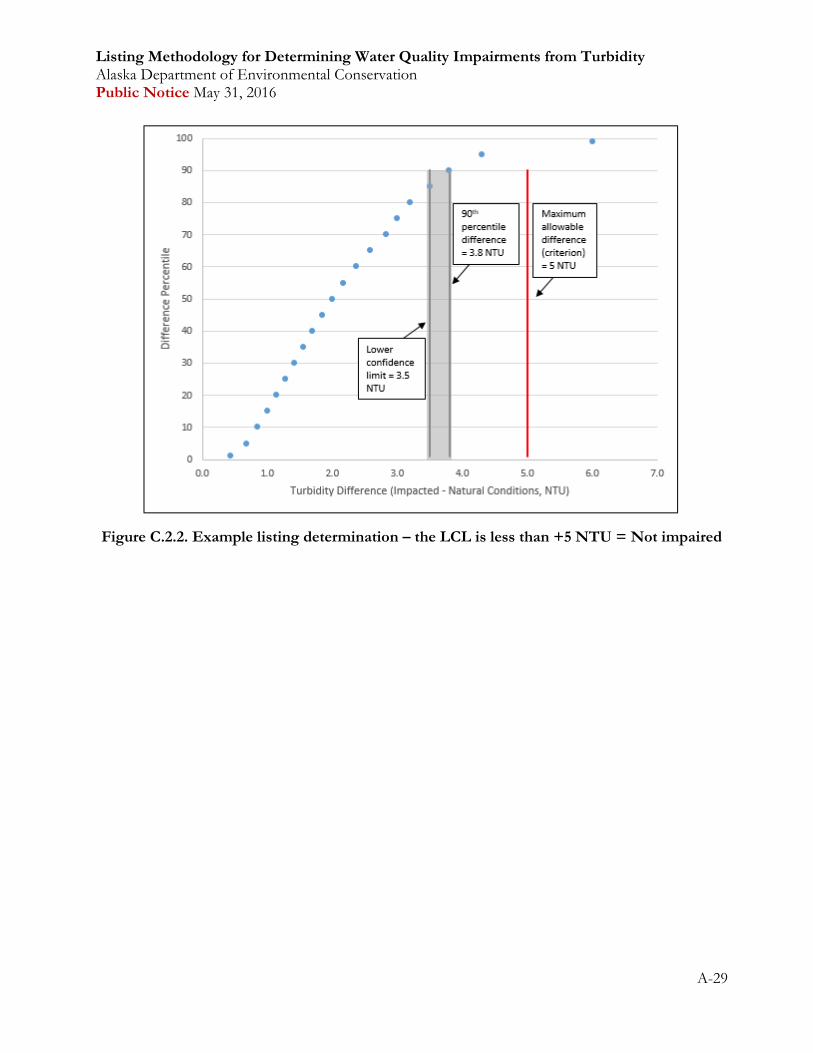
Listing Methodology for Determining Water Quality Impairments from Turbidity Alaska Department of Environmental Conservation Public Notice May 31, 2016
A-29
Figure C.2.2. Example listing determination – the LCL is less than +5 NTU = Not impaired

Listing Methodology for Determining Water Quality Impairments from Turbidity Alaska Department of Environmental Conservation Public Notice May 31, 2016
A-30
Figure C.2.3. Example attainment determination – the UCL is greater than +5 NTU = Not attaining

Listing Methodology for Determining Water Quality Impairments from Turbidity Alaska Department of Environmental Conservation Public Notice May 31, 2016
A-31
Figure C.2.4. Example attainment determination – the UCL is less than +5 NTU = Attaining
C.3 References
DEC. 2016. ADEC Turbidity Hypothesis Tests Template., dated March 31, 2016. [website TBD]


