Download - LESSON 10 & 11 SIMPLE LINEAR REGRESSION
LESSON 10 & 11
SIMPLE LINEAR REGRESSION
SAMIE L.S. LY
1

2
1. Simple Linear Regression Model
2. Least Square Method
3. Coefficient of Determination
4. Model Assumptions
5. Testing for Significance
6. Covariance & Coefficient of Correlation
7. Using the Estimated Regression –Equation for Estimation and Prediction
S.L.S.Ly
C215
SIMPLE LINEAR REGRESSION MODEL
REGRESSION MODEL
REGRESSION EQUATION
ESTIMATED REGRESSION EQUATION
3

S.L.S.Ly
C215
THE OBJECTIVE OF SLR
Let’s say, I would like to create the ultimate equation to figure
out my Final COMM 215 grade.
What influences my Final COMM 215 grade?
Think of a few examples.
4

S.L.S.Ly
C215
FINAL COMM 215 Grade (y) =
Study Time (x1) +
Work Time (x2) +
# of hours spent on Facebook (x3) +
Family Time (x4) +
anything else you can think of (x…) …
5

S.L.S.Ly
C215
THE OBJECTIVE OF SLR
Let’s say, I would like to create the ultimate equation to figure
out my Final COMM 215 grade.
Let’s say,
I study 5 hours a week,
work part-time for 25 hours a week,
I spend 3 hours on facebook,
And I have 2 kids.
Here is 1 scenario.
6
S.L.S.Ly
C215
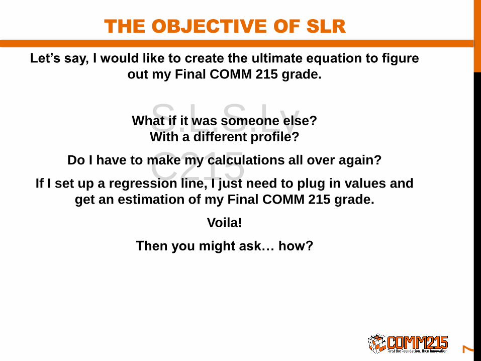
THE OBJECTIVE OF SLR
Let’s say, I would like to create the ultimate equation to figure
out my Final COMM 215 grade.
What if it was someone else?
With a different profile?
Do I have to make my calculations all over again?
If I set up a regression line, I just need to plug in values and
get an estimation of my Final COMM 215 grade.
Voila!
Then you might ask… how?
7

S.L.S.Ly
C215
THE OBJECTIVE OF SLR
Let’s say, I would like to create the ultimate equation to figure
out my Final COMM 215 grade.
How do I create this regression line?
Answer: By gathering data from history.
I am going to take a sample of individuals who took COMM
215 before and write down their profile.
Hours per
week
Study Time Work Time Family
Time
Time
Bob 10 25 5 0
Sally 12 0 15 15
Eric 3 40 10 0
8

S.L.S.Ly
C215
THE OBJECTIVE OF SLR
Let’s say, I would like to create the ultimate equation to figure
out my Final COMM 215 grade.
Since we are only considering 1 independent variable, let’s
take just 1, Study Time as the main indicator of your Final
COMM 215 grade.
Hours per
week
Study Time(x) Final Grade(y)
Bob 10 89
Sally 12 67
Eric 3 45
9
S.L.S.Ly
C215
THE OBJECTIVE OF SLR
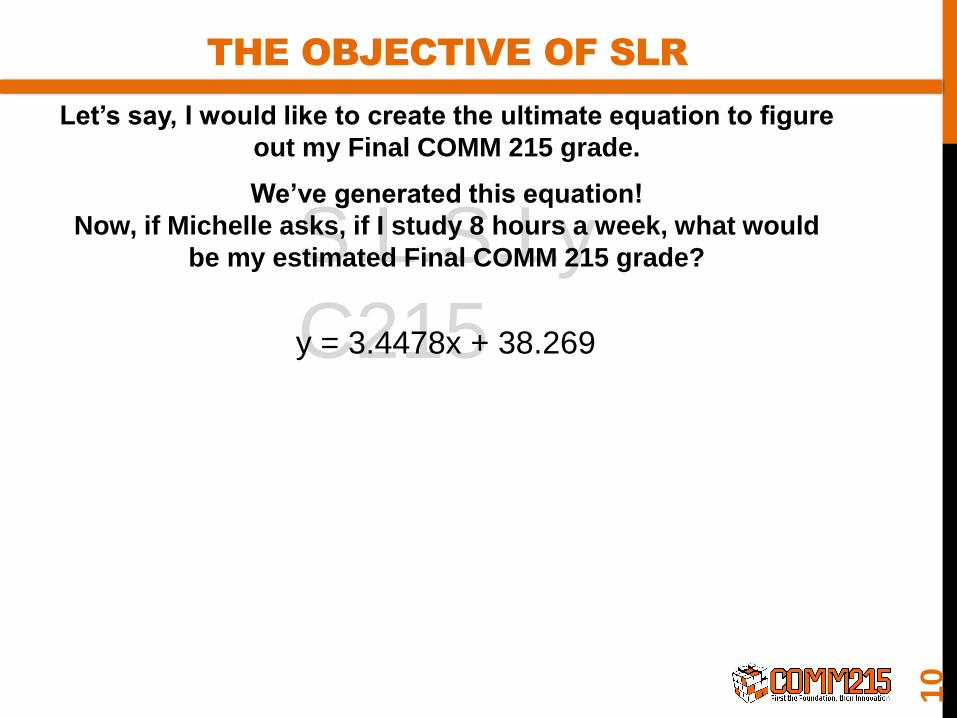
Let’s say, I would like to create the ultimate equation to figure
out my Final COMM 215 grade.
We’ve generated this equation!
Now, if Michelle asks, if I study 8 hours a week, what would
be my estimated Final COMM 215 grade?
y = 3.4478x + 38.269
10
S.L.S.Ly
C215
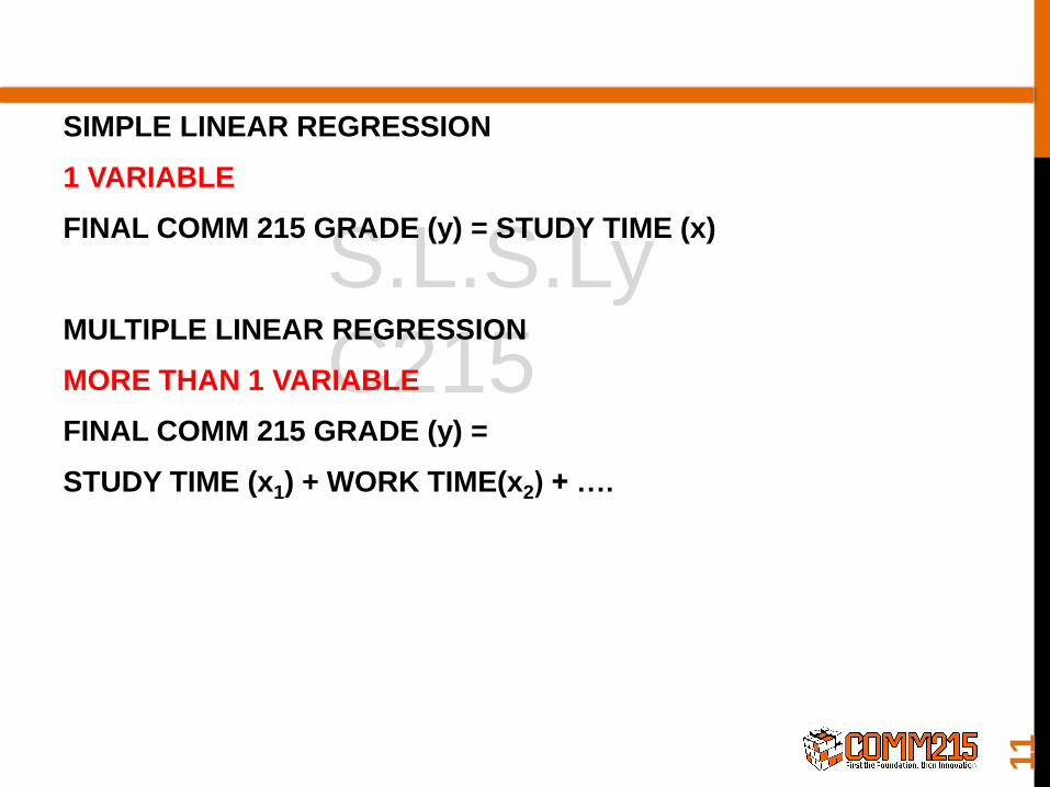
SIMPLE LINEAR REGRESSION
1 VARIABLE
FINAL COMM 215 GRADE (y) = STUDY TIME (x)
MULTIPLE LINEAR REGRESSION
MORE THAN 1 VARIABLE
FINAL COMM 215 GRADE (y) =
STUDY TIME (x1) + WORK TIME(x2) + ….
11
S.L.S.Ly
C215
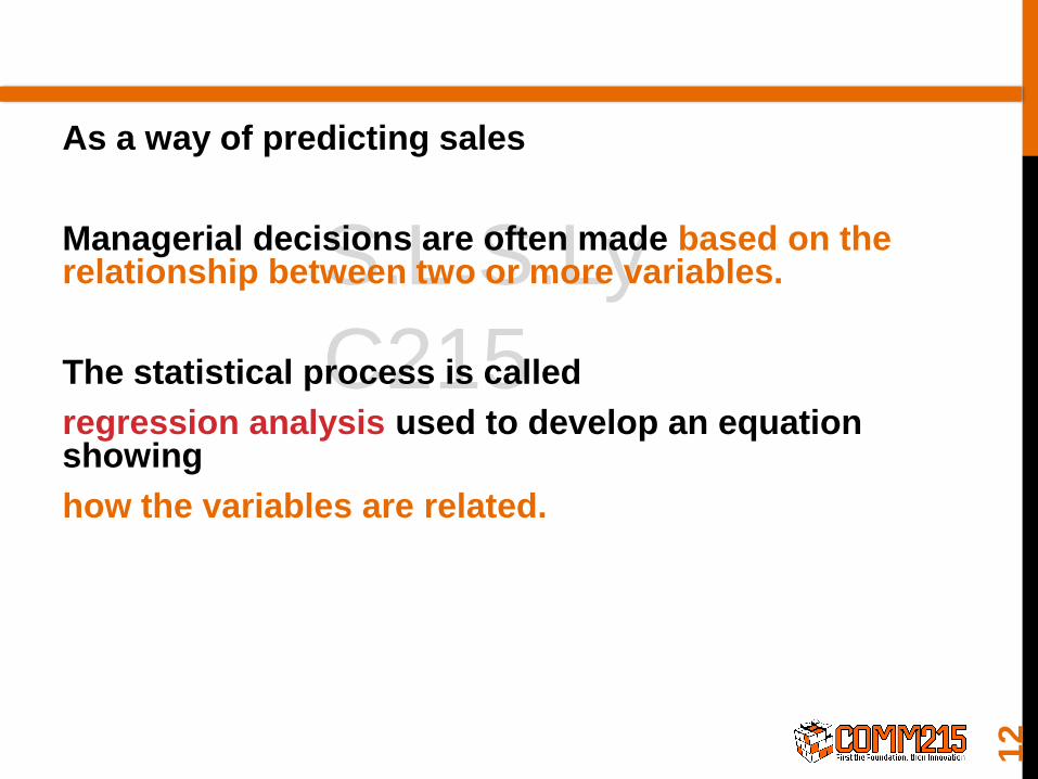
As a way of predicting sales
Managerial decisions are often made based on the relationship between two or more variables.
The statistical process is called
regression analysis used to develop an equation showing
how the variables are related.
12

S.L.S.Ly
C215
The variable
being predicted is
called the dependent variable.
The variable or variables
being used to predict the value of the dependence variable are
called independent variables.
13
S.L.S.Ly
C215
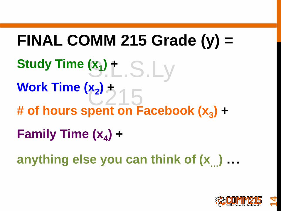
FINAL COMM 215 Grade (y) =
Study Time (x1) +
Work Time (x2) +
# of hours spent on Facebook (x3) +
Family Time (x4) +
anything else you can think of (x…) …
14

SIMPLE LINEAR REGRESSION
EQUATION
Positive Linear Relationship
E(y)
x
Slope b1
is positive
Regression line
Interceptb0
The relationship between the two variables is approximated by a straight line.
15Bowerman, et al. (2017) pp. 534
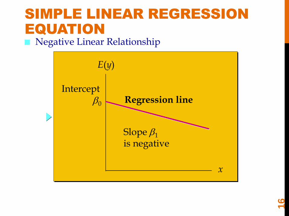
Negative Linear Relationship
E(y)
x
Slope b1
is negative
Regression lineIntercept
b0
SIMPLE LINEAR REGRESSION
EQUATION
16
S.L.S.Ly
C215
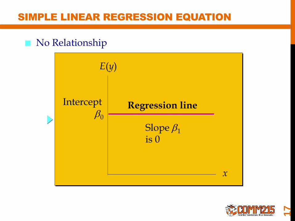
No Relationship
E(y)
x
Slope b1
is 0
Regression lineInterceptb0
SIMPLE LINEAR REGRESSION EQUATION
17
S.L.S.Ly
C215
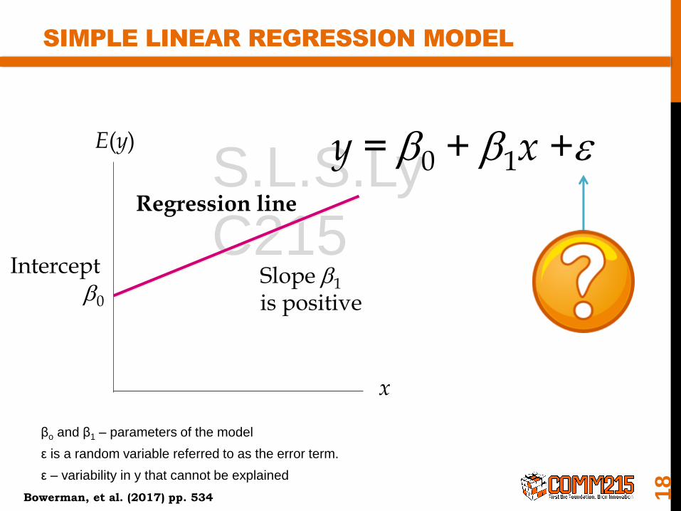
SIMPLE LINEAR REGRESSION MODEL
βo and β1 – parameters of the model
ε is a random variable referred to as the error term.
ε – variability in y that cannot be explained
y = b0 + b1x +eE(y)
x
Slope b1
is positive
Regression line
Interceptb0
18
Bowerman, et al. (2017) pp. 534
S.L.S.Ly
C215
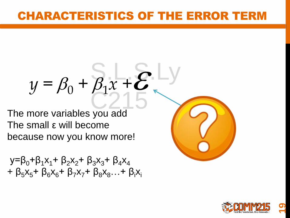
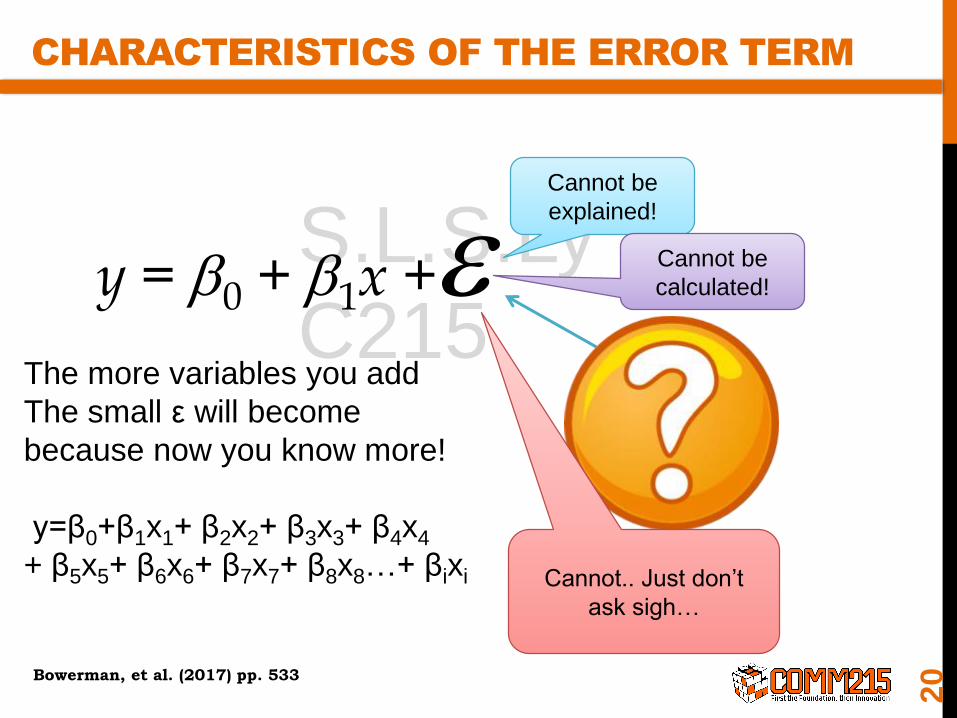
CHARACTERISTICS OF THE ERROR TERM
y = b0 + b1x +eThe more variables you add
The small ε will become
because now you know more!
y=β0+β1x1+ β2x2+ β3x3+ β4x4
+ β5x5+ β6x6+ β7x7+ β8x8…+ βixi
19
S.L.S.Ly
C215
CHARACTERISTICS OF THE ERROR TERM
y = b0 + b1x +eThe more variables you add
The small ε will become
because now you know more!
y=β0+β1x1+ β2x2+ β3x3+ β4x4
+ β5x5+ β6x6+ β7x7+ β8x8…+ βixi
Cannot be
explained!
Cannot be
calculated!
Cannot.. Just don’t
ask sigh…
20Bowerman, et al. (2017) pp. 533

S.L.S.Ly
C215
REGRESSION EQUATION
Describes how the expected value of y, E(y) is related to x
21
E(y) = b0 + b1x
• E(y) is the expected value of y for a given x value.
• b1 is the slope of the regression line.
• b0 is the y intercept of the regression line.
• Graph of the regression equation is a straight line.
Bowerman, et al. (2017) pp. 535

S.L.S.Ly
C215
ESTIMATED SIMPLE LINEAR REGRESSION EQUATION
Sample statistics are
22
E(y) = b0 + b1x
0 1y b b x
• is the estimated value of y for a given x value.y
• b1 is the slope of the line.
• b0 is the y intercept of the line.
• The graph is called the estimated regression line.
Bowerman, et al. (2017) pp. 535
S.L.S.Ly
C215
PROBLEM #10.1
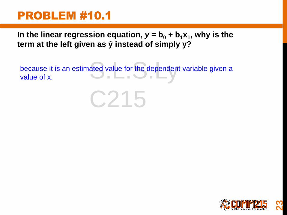
In the linear regression equation, y = b0 + b1x1, why is the
term at the left given as ŷ instead of simply y?
because it is an estimated value for the dependent variable given a
value of x.
23
24
Least Square Method
Coefficient of Determination
Model Assumptions
Testing for Significance
Covariance & Coefficient of Correlation
Using the Estimated Regression –Equation for Estimation and Prediction
S.L.S.Ly
C215
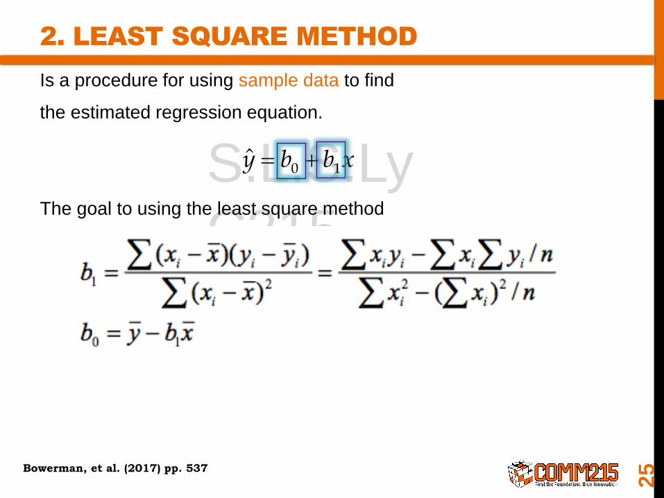
2. LEAST SQUARE METHOD
Is a procedure for using sample data to find
the estimated regression equation.
The goal to using the least square method
25
0 1y b b x
Bowerman, et al. (2017) pp. 537
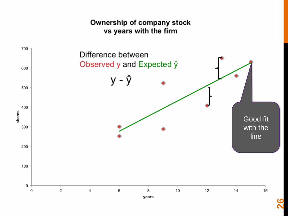
Good fit
with the
line
26

S.L.S.Ly
C215
LEAST SQUARES METHOD
Least Squares Criterion
27
min (y yi i )2
where:
yi = observed value of the dependent variable
for the ith observation^yi = estimated value of the dependent variable
for the ith observation
Bowerman, et al. (2017) pp. 536
S.L.S.Ly
C215
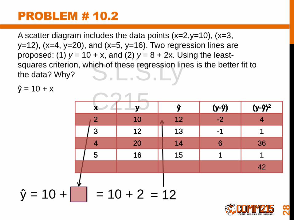
PROBLEM # 10.2
A scatter diagram includes the data points (x=2,y=10), (x=3,
y=12), (x=4, y=20), and (x=5, y=16). Two regression lines are
proposed: (1) y = 10 + x, and (2) y = 8 + 2x. Using the least-
squares criterion, which of these regression lines is the better fit to
the data? Why?
ŷ = 10 + x
28
x y ŷ (y-ŷ) (y-ŷ)2x y ŷ (y-ŷ) (y-ŷ)2
2 10
3 12
4 20
5 16
ŷ = 10 + = 10 + 2 = 12
x y ŷ (y-ŷ) (y-ŷ)2
2 10 12
3 12
4 20
5 16
x y ŷ (y-ŷ) (y-ŷ)2
2 10 12
3 12 13
4 20 14
5 16 15
x y ŷ (y-ŷ) (y-ŷ)2
2 10 12 -2
3 12 13 -1
4 20 14 6
5 16 15 1
x y ŷ (y-ŷ) (y-ŷ)2
2 10 12 -2 4
3 12 13 -1 1
4 20 14 6 36
5 16 15 1 1
x y ŷ (y-ŷ) (y-ŷ)2
2 10 12 -2 4
3 12 13 -1 1
4 20 14 6 36
5 16 15 1 1
42
S.L.S.Ly
C215
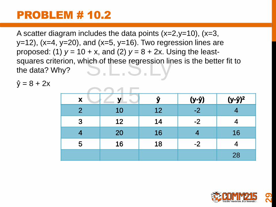
PROBLEM # 10.2
A scatter diagram includes the data points (x=2,y=10), (x=3,
y=12), (x=4, y=20), and (x=5, y=16). Two regression lines are
proposed: (1) y = 10 + x, and (2) y = 8 + 2x. Using the least-
squares criterion, which of these regression lines is the better fit to
the data? Why?
ŷ = 8 + 2x
29
x y ŷ (y-ŷ) (y-ŷ)2
2 10
3 12
4 20
5 16
x y ŷ (y-ŷ) (y-ŷ)2
2 10 12
3 12 14
4 20 16
5 16 18
x y ŷ (y-ŷ) (y-ŷ)2
2 10 12 -2
3 12 14 -2
4 20 16 4
5 16 18 -2
x y ŷ (y-ŷ) (y-ŷ)2
2 10 12 -2 4
3 12 14 -2 4
4 20 16 4 16
5 16 18 -2 4
x y ŷ (y-ŷ) (y-ŷ)2
2 10 12 -2 4
3 12 14 -2 4
4 20 16 4 16
5 16 18 -2 4
28
S.L.S.Ly
C215
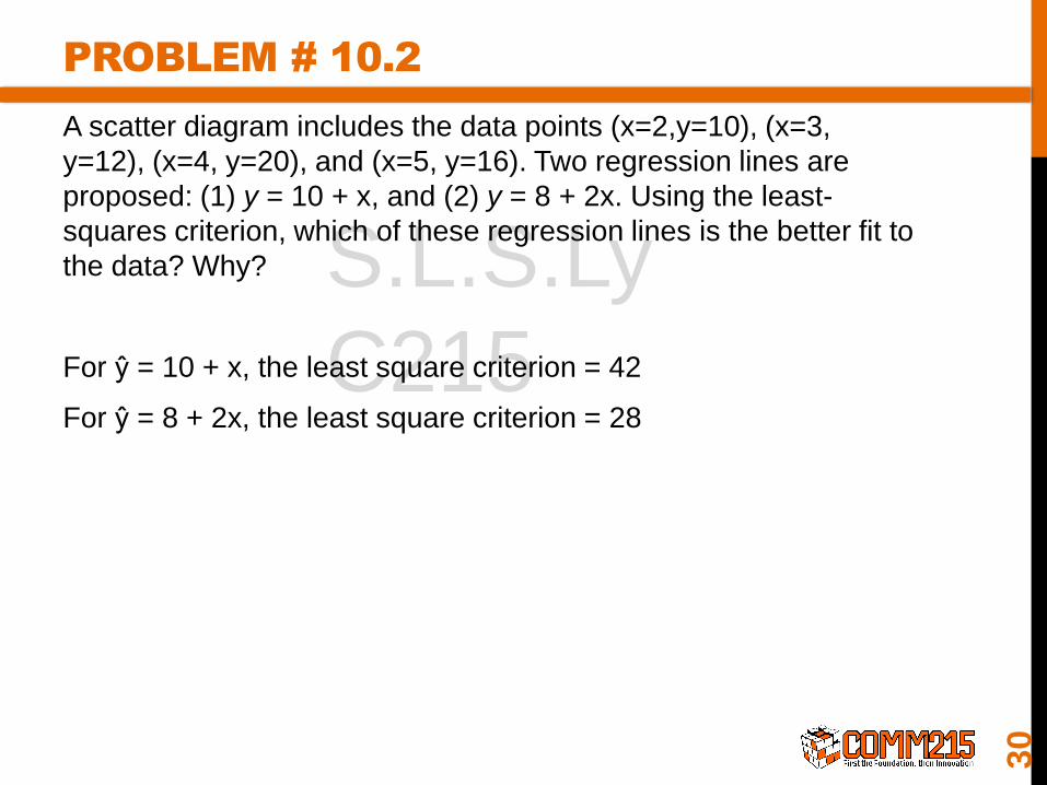
PROBLEM # 10.2
A scatter diagram includes the data points (x=2,y=10), (x=3,
y=12), (x=4, y=20), and (x=5, y=16). Two regression lines are
proposed: (1) y = 10 + x, and (2) y = 8 + 2x. Using the least-
squares criterion, which of these regression lines is the better fit to
the data? Why?
For ŷ = 10 + x, the least square criterion = 42
For ŷ = 8 + 2x, the least square criterion = 28
30

S.L.S.Ly
C215
LEAST SQUARES METHOD
Slope for the Estimated Regression Equation
31
1 2
( )( )
( )i i
i
x x y yb
x x
where:xi = value of independent variable for ith
observation
_y = mean value for dependent variable
_x = mean value for independent variable
yi = value of dependent variable for ithobservation
Bowerman, et al. (2017) pp. 536

S.L.S.Ly
C215
y-Intercept for the Estimated Regression Equation
0 1b y b x
LEAST SQUARES METHOD
32
S.L.S.Ly
C215
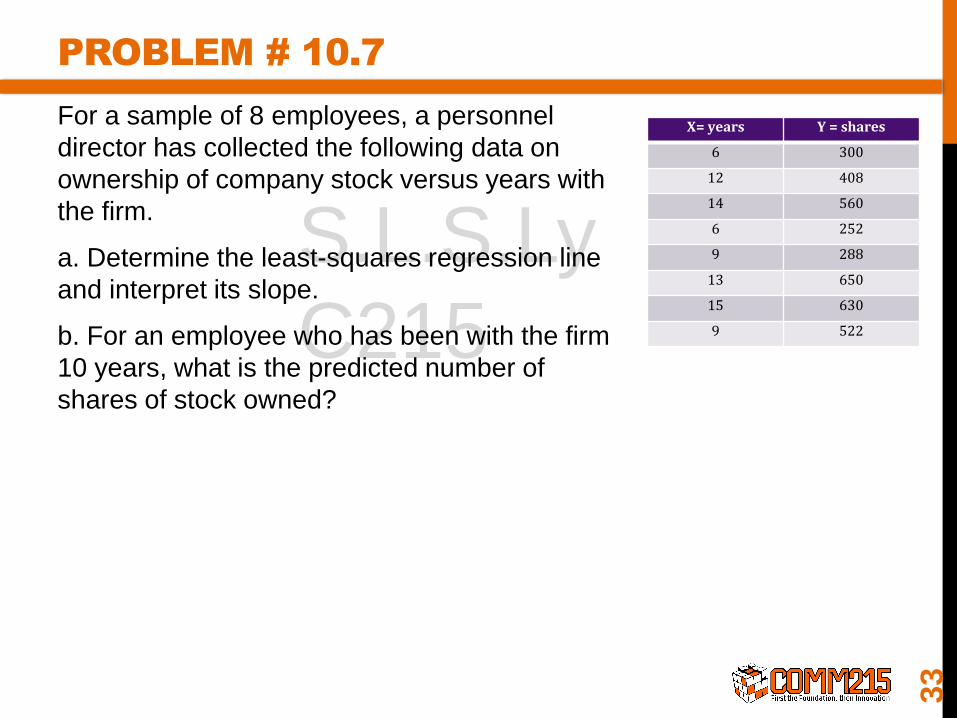
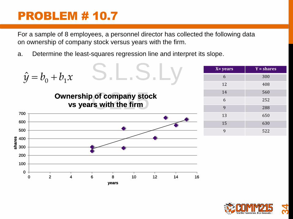
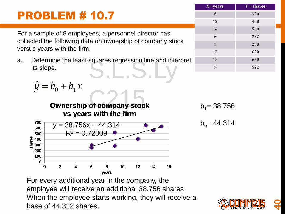
PROBLEM # 10.7
For a sample of 8 employees, a personnel
director has collected the following data on
ownership of company stock versus years with
the firm.
a. Determine the least-squares regression line
and interpret its slope.
b. For an employee who has been with the firm
10 years, what is the predicted number of
shares of stock owned?
33
X= years Y = shares
6 300
12 408
14 560
6 252
9 288
13 650
15 630
9 522
S.L.S.Ly
C215
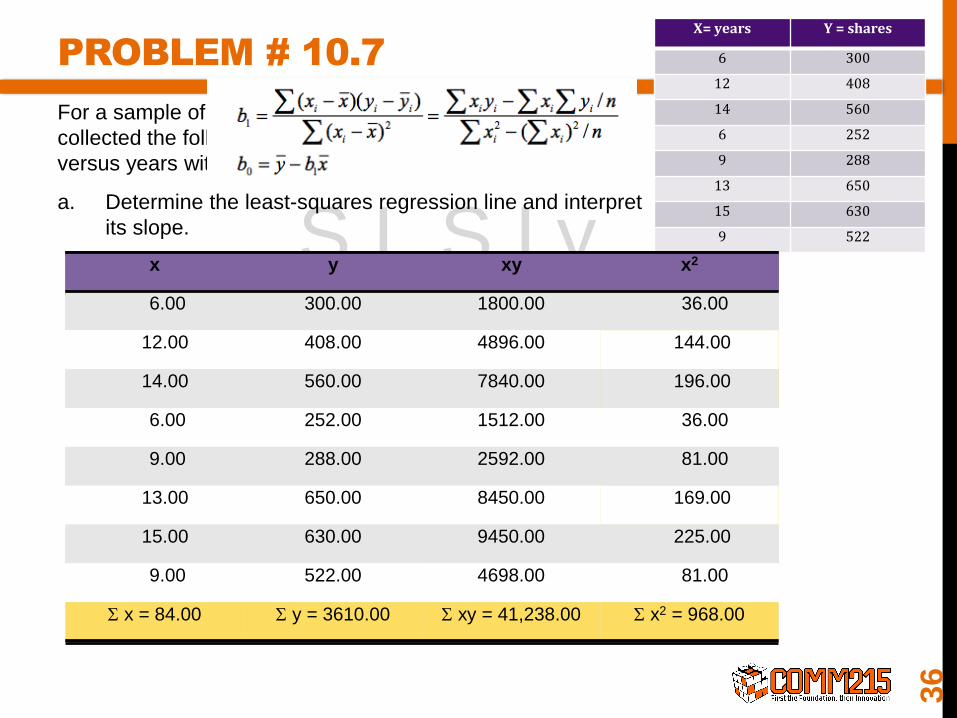
PROBLEM # 10.7
For a sample of 8 employees, a personnel director has collected the following data
on ownership of company stock versus years with the firm.
a. Determine the least-squares regression line and interpret its slope.
34
X= years Y = shares
6 300
12 408
14 560
6 252
9 288
13 650
15 630
9 522
0
100
200
300
400
500
600
700
0 2 4 6 8 10 12 14 16
sh
are
s
years
Ownership of company stock vs years with the firm
0
100
200
300
400
500
600
700
0 2 4 6 8 10 12 14 16
sh
are
s
years
Ownership of company stock vs years with the firm
0 1y b b x

S.L.S.Ly
C215
PROBLEM # 10.7
For a sample of 8 employees, a personnel director has
collected the following data on ownership of company stock
versus years with the firm.
a. Determine the least-squares regression line and interpret
its slope.
35
X= years Y = shares
6 300
12 408
14 560
6 252
9 288
13 650
15 630
9 522
0 1y b b x
S.L.S.Ly
C215 x y xy x2
6.00 300.00 1800.00 36.00
12.00 408.00 4896.00 144.00
14.00 560.00 7840.00 196.00
6.00 252.00 1512.00 36.00
9.00 288.00 2592.00 81.00
13.00 650.00 8450.00 169.00
15.00 630.00 9450.00 225.00
9.00 522.00 4698.00 81.00
x = 84.00 y = 3610.00 xy = 41,238.00 x2 = 968.00
x y xy x2
6.00 300.00 1800.00 36.00
12.00 408.00 4896.00
14.00 560.00
6.00 252.00 1512.00 36.00
9.00 288.00 81.00
13.00 650.00 8450.00
15.00 630.00 9450.00 225.00
9.00 522.00 81.00
x = y = xy = x2 =
PROBLEM # 10.7
For a sample of 8 employees, a personnel director has
collected the following data on ownership of company stock
versus years with the firm.
a. Determine the least-squares regression line and interpret
its slope.
36
X= years Y = shares
6 300
12 408
14 560
6 252
9 288
13 650
15 630
9 522
x y xy x2
6.00 300.00 1800.00 36.00
12.00 408.00 4896.00
14.00 560.00 7840.00
6.00 252.00 1512.00 36.00
9.00 288.00 2592.00 81.00
13.00 650.00 8450.00
15.00 630.00 9450.00 225.00
9.00 522.00 4698.00 81.00
x = y = xy = x2 =
x y xy x2
6.00 300.00 1800.00 36.00
12.00 408.00 4896.00 144.00
14.00 560.00 7840.00 196.00
6.00 252.00 1512.00 36.00
9.00 288.00 2592.00 81.00
13.00 650.00 8450.00 169.00
15.00 630.00 9450.00 225.00
9.00 522.00 4698.00 81.00
x = y = xy = x2 =
x y xy x2
6.00 300.00 1800.00 36.00
12.00 408.00 4896.00 144.00
14.00 560.00 7840.00 196.00
6.00 252.00 1512.00 36.00
9.00 288.00 2592.00 81.00
13.00 650.00 8450.00 169.00
15.00 630.00 9450.00 225.00
9.00 522.00 4698.00 81.00
x = 84.00 y = 3610.00 xy = 41,238.00 x2 = 968.00
S.L.S.Ly
C215
PROBLEM # 10.7
For a sample of 8 employees, a personnel director has collected the following data
on ownership of company stock versus years with the firm.
a. Determine the least-squares regression line and interpret its slope.
37
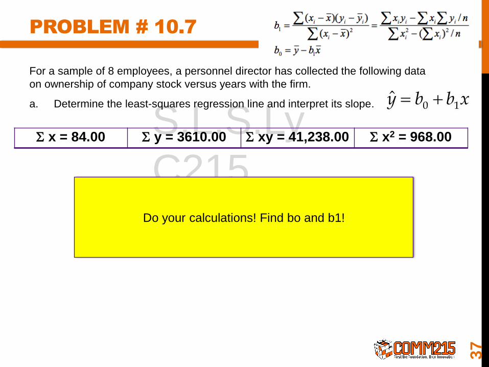
0 1y b b x
x = 84.00 y = 3610.00 xy = 41,238.00 x2 = 968.00
Do your calculations! Find bo and b1!

S.L.S.Ly
C215
PROBLEM # 10.7
For a sample of 8 employees, a personnel director has collected the following data
on ownership of company stock versus years with the firm.
a. Determine the least-squares regression line and interpret its slope.
38
0 1y b b x
x = 84.00 y = 3610.00 xy = 41,238.00 x2 = 968.00
b1=Σxy –[Σx Σy / n]
Σx2 – [(Σx)2 / n]
41,238 – [(84) (3610)/8]
(968) – [(84)2 / 8]=
3333
86= = 38.756
S.L.S.Ly
C215
PROBLEM # 10.7
For a sample of 8 employees, a personnel director has collected the following data
on ownership of company stock versus years with the firm.
a. Determine the least-squares regression line and interpret its slope.
39
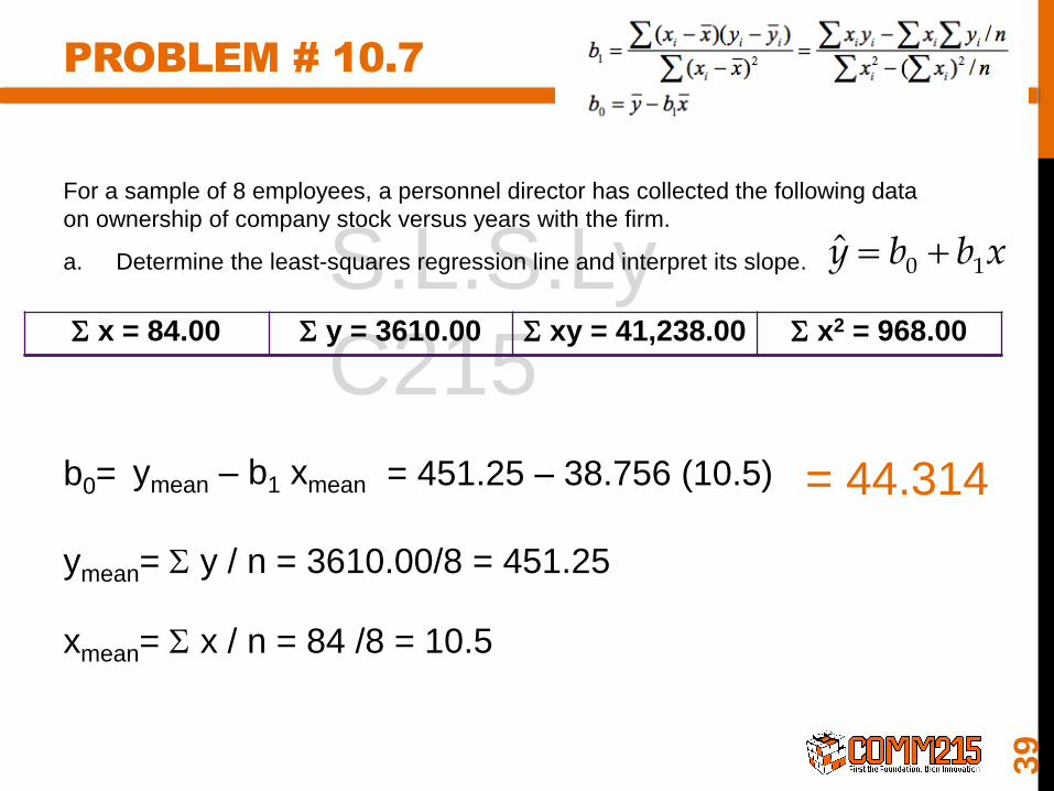
0 1y b b x
x = 84.00 y = 3610.00 xy = 41,238.00 x2 = 968.00
b0= ymean – b1 xmean = 451.25 – 38.756 (10.5)
ymean= y / n = 3610.00/8 = 451.25
xmean= x / n = 84 /8 = 10.5
= 44.314
S.L.S.Ly
C215
PROBLEM # 10.7
For a sample of 8 employees, a personnel director has
collected the following data on ownership of company stock
versus years with the firm.
a. Determine the least-squares regression line and interpret
its slope.
40
X= years Y = shares
6 300
12 408
14 560
6 252
9 288
13 650
15 630
9 522
0
100
200
300
400
500
600
700
0 2 4 6 8 10 12 14 16
sh
are
s
years
Ownership of company stock vs years with the firm
0
100
200
300
400
500
600
700
0 2 4 6 8 10 12 14 16
sh
are
s
years
Ownership of company stock vs years with the firm
0 1y b b x
y = 38.756x + 44.314R² = 0.72009
0
100
200
300
400
500
600
700
0 2 4 6 8 10 12 14 16
sh
are
s
years
Ownership of company stock vs years with the firm
b1= 38.756
bo= 44.314
For every additional year in the company, the
employee will receive an additional 38.756 shares.
When the employee starts working, they will receive a
base of 44.312 shares.
S.L.S.Ly
C215
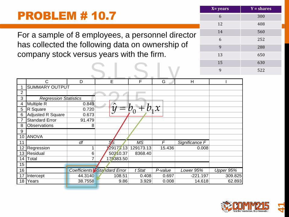
PROBLEM # 10.7
For a sample of 8 employees, a personnel director
has collected the following data on ownership of
company stock versus years with the firm.
41
X= years Y = shares
6 300
12 408
14 560
6 252
9 288
13 650
15 630
9 522
1
2
3
4
5
6
7
8
9
10
11
12
13
14
15
16
17
18
C D E F G H I
SUMMARY OUTPUT
Regression Statistics
Multiple R 0.849
R Square 0.720
Adjusted R Square 0.673
Standard Error 91.479
Observations 8
ANOVA
df SS MS F Significance F
Regression 1 129173.13 129173.13 15.436 0.008
Residual 6 50210.37 8368.40
Total 7 179383.50
Coefficients Standard Error t Stat P-value Lower 95% Upper 95%
Intercept 44.3140 108.51 0.408 0.697 -221.197 309.825
Years 38.7558 9.86 3.929 0.008 14.618 62.893
0 1y b b x

S.L.S.Ly
C215
PROBLEM # 10.7
For a sample of 8 employees, a personnel director
has collected the following data on ownership of
company stock versus years with the firm.
b. For an employee who has been with the firm
10 years, what is the predicted number of shares of
stock owned?
42
X= years Y = shares
6 300
12 408
14 560
6 252
9 288
13 650
15 630
9 522
ŷ = 44.314 + 38.756 x
ŷ = 44.314 + 38.756 (10)
ŷ = 431.9
the predicted value of Shares will be 431.9
43
Coefficient of Determination
Model Assumptions
Testing for Significance
Covariance & Coefficient of Correlation
Using the Estimated Regression –Equation for Estimation and Prediction
S.L.S.Ly
C215
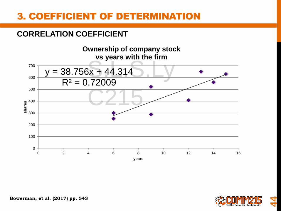
3. COEFFICIENT OF DETERMINATION
CORRELATION COEFFICIENT
44
y = 38.756x + 44.314R² = 0.72009
0
100
200
300
400
500
600
700
0 2 4 6 8 10 12 14 16
sh
are
s
years
Ownership of company stock vs years with the firm
Bowerman, et al. (2017) pp. 543
S.L.S.Ly
C215
COEFFICIENT OF DETERMINATION
0
100
200
300
400
500
600
700
0 2 4 6 8 10 12 14 16 18
SH
AR
ES
YEARS
Ownership of company stock vs years with the firm
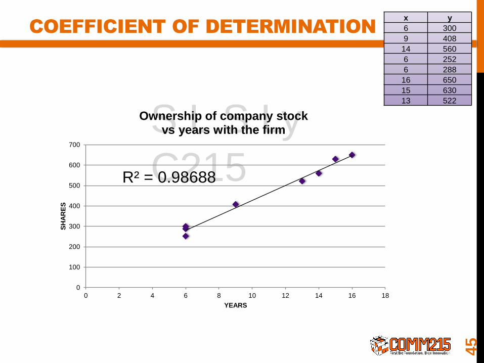
x y
6 300
9 408
14 560
6 252
6 288
16 650
15 630
13 522
R² = 0.98688
45
S.L.S.Ly
C215
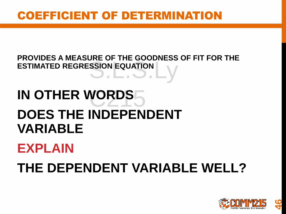
COEFFICIENT OF DETERMINATION
PROVIDES A MEASURE OF THE GOODNESS OF FIT FOR THE ESTIMATED REGRESSION EQUATION
IN OTHER WORDS
DOES THE INDEPENDENT VARIABLE
EXPLAIN
THE DEPENDENT VARIABLE WELL?
46

47
FINAL COMM 215 Grade (y) =
Study Time (x1) +
Work Time (x2) +
# of hours spent on Facebook
(x3) +
Family Time (x4) +
anything else you can think of
(x…) …
Explain 40% of
the grade
Explain 15% of
the grade
Explain 9% of
the grade
Explain 15% of
the grade
These 4 Variables
explain
79% of your
grade!
S.L.S.Ly
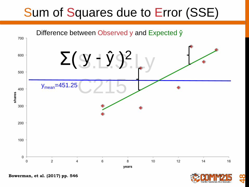
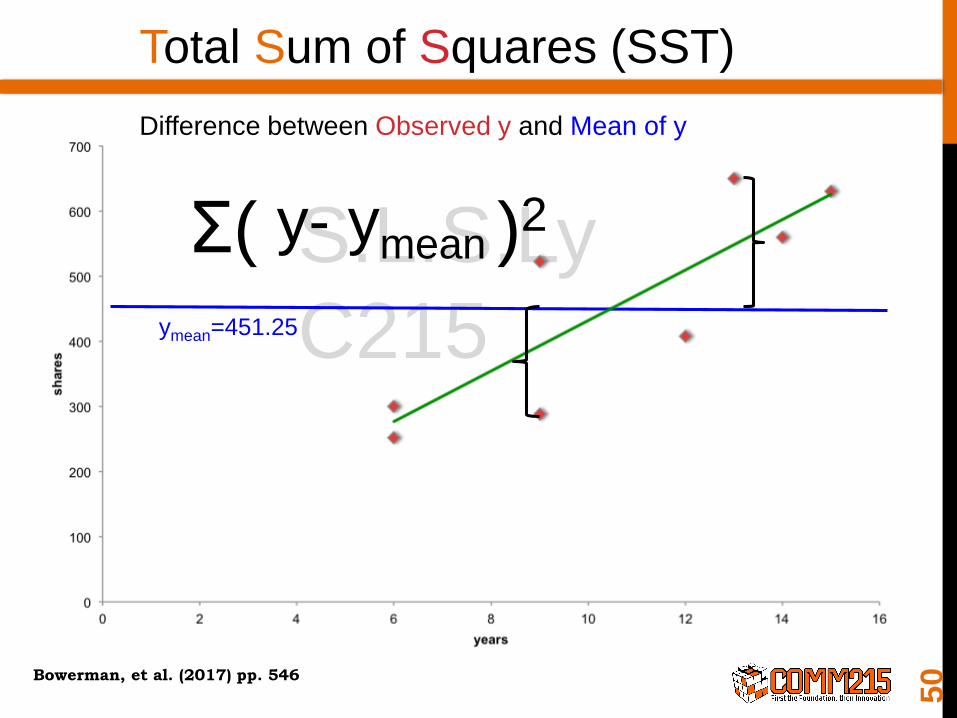
C215 ymean=451.25
Sum of Squares due to Error (SSE)
Difference between Observed y and Expected ŷ
y - ŷΣ( )2
48Bowerman, et al. (2017) pp. 546
S.L.S.Ly
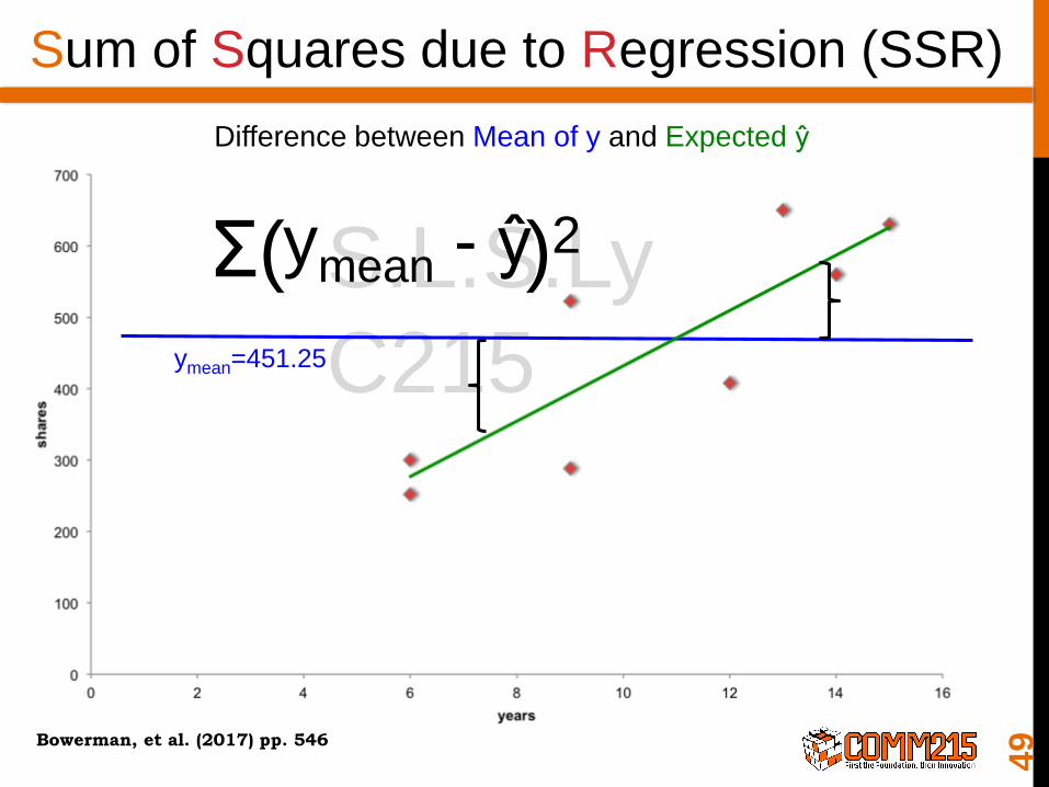
C215 ymean=451.25
Sum of Squares due to Regression (SSR)
Difference between Mean of y and Expected ŷ
ymean - ŷΣ( )2
49Bowerman, et al. (2017) pp. 546
S.L.S.Ly
C215 ymean=451.25
Total Sum of Squares (SST)
Difference between Observed y and Mean of y
y- ymeanΣ( )2
50Bowerman, et al. (2017) pp. 546
S.L.S.Ly
C215
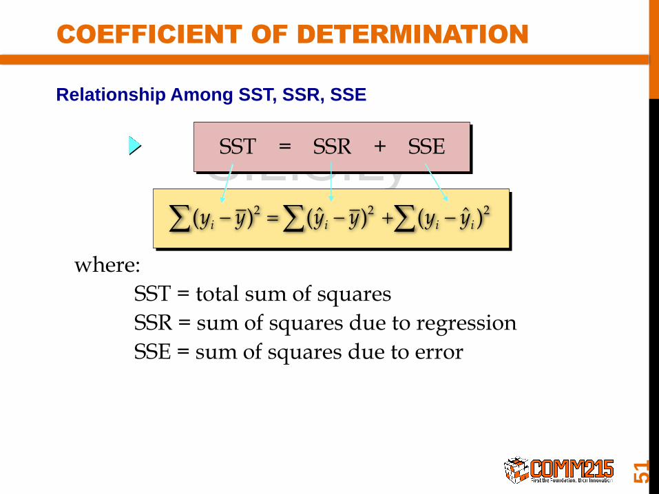
COEFFICIENT OF DETERMINATION
Relationship Among SST, SSR, SSE
where:
SST = total sum of squares
SSR = sum of squares due to regression
SSE = sum of squares due to error
SST = SSR + SSE
2( )iy y 2ˆ( )iy y 2ˆ( )i iy y
51

The coefficient of determination is:
where:
SSR = sum of squares due to regression= explained variation
SST = total sum of squares
= total variation
r2 = SSR/SST
COEFFICIENT OF DETERMINATION
52Bowerman, et al. (2017) pp. 545

COEFFICIENT OF
DETERMINATION (R2)
Expresses proportion of
the variation in the
dependent variable (y)
that is explained by the
regression line:
ŷ = b0+b1x1
COEFFICIENT OF
CORRELATION (R)
Describes both the
direction and the
strength of the linear
relationship between
two variables
r = (sign of b1) √ r2
53Bowerman, et al. (2017) pp. 546
S.L.S.Ly
C215
PROBLEM #10.9
For a set of data, the total variation or sum of squares for y is
SST = 143.0, and error sum of squares is SSE = 24.0. What
proportion of the variation in y is explained by the regression
equation?
54

S.L.S.Ly
C215
PROBLEM #10.9
For a set of data, the total variation or sum of squares for y is
SST = 143.0, and error sum of squares is SSE = 24.0. What
proportion of the variation in y is explained by the regression
equation?
= SSR/SST
We are asked to find the
coefficient of determination :
R2
We also know SST = SSR + SSE
55
S.L.S.Ly
C215
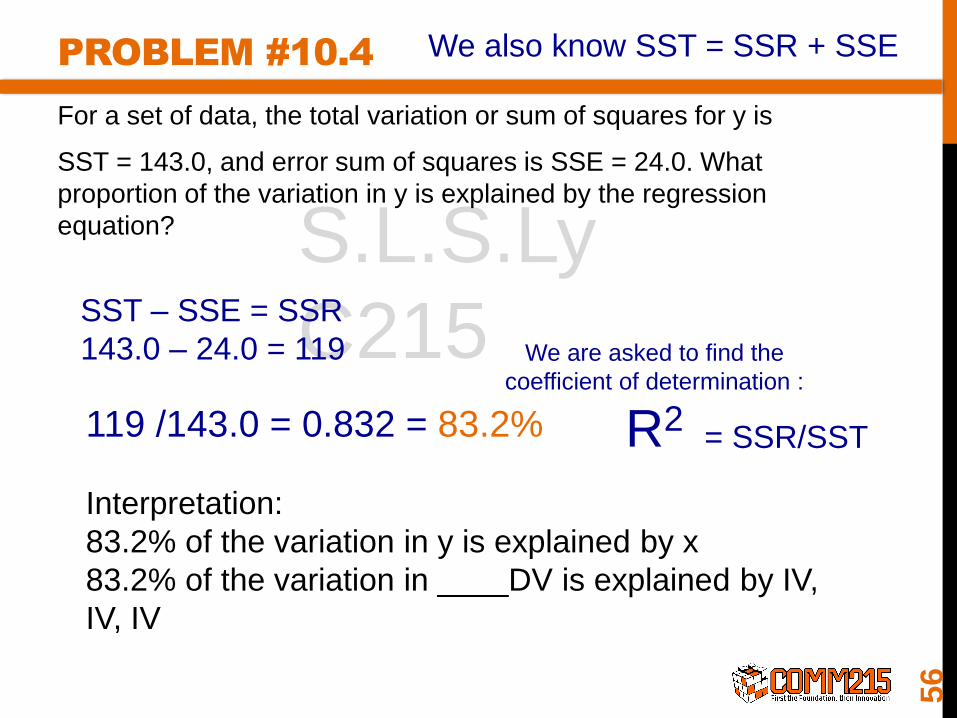
PROBLEM #10.4
For a set of data, the total variation or sum of squares for y is
SST = 143.0, and error sum of squares is SSE = 24.0. What
proportion of the variation in y is explained by the regression
equation?
= SSR/SST
We are asked to find the
coefficient of determination :
R2
We also know SST = SSR + SSE
SST – SSE = SSR
143.0 – 24.0 = 119
119 /143.0 = 0.832 = 83.2%
Interpretation:
83.2% of the variation in y is explained by x
83.2% of the variation in ____DV is explained by IV,
IV, IV
56

57
Model Assumptions
Testing for Significance
Covariance & Coefficient of Correlation
Using the Estimated Regression –Equation for Estimation and Prediction

S.L.S.Ly
C215
4. MODEL ASSUMPTIONS
Before conducting regression analysis…
What determines an appropriate model for
the relationship between the dependent
and the independent variable(s).
58

S.L.S.Ly
C215
Even if the data fits well , the estimated
regression equation should not be used
until further analysis of
how appropriate the assumed model is.
One way to determine is to test for
significance.
59
S.L.S.Ly
C215
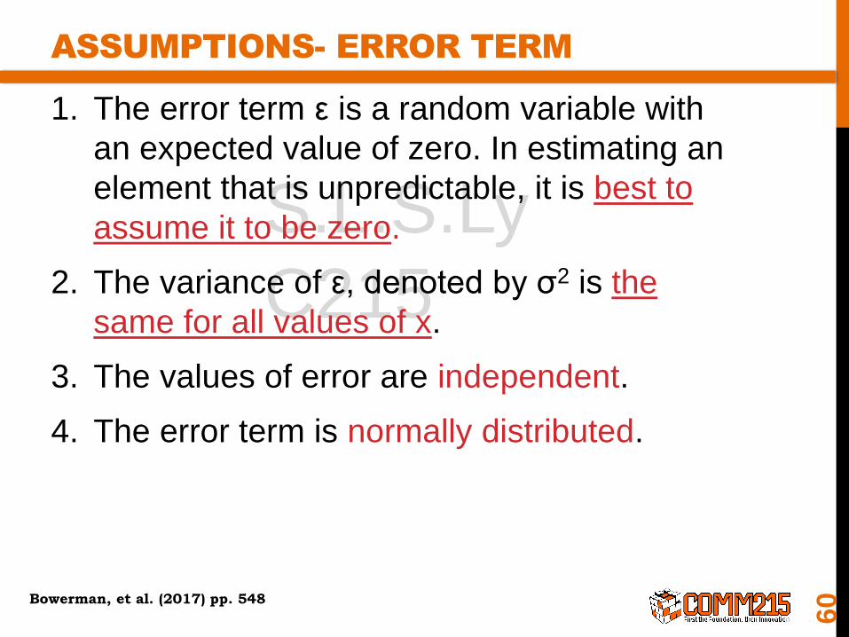
ASSUMPTIONS- ERROR TERM
1. The error term ε is a random variable with
an expected value of zero. In estimating an
element that is unpredictable, it is best to
assume it to be zero.
2. The variance of ε, denoted by σ2 is the
same for all values of x.
3. The values of error are independent.
4. The error term is normally distributed.
60Bowerman, et al. (2017) pp. 548

S.L.S.Ly
C215
Do you see the normal curve?
61

S.L.S.Ly
C215
Do you see the normal curve?
Right here is the population
mean, which is also your point
on the line.
62

S.L.S.Ly
C215
Assumption # 2: The variance/ standard
deviation for each value x is the same. All
of these normal distributions have the
same standard deviation.
Assumption # 2: The variance/ standard
deviation for each value x is the same. All
of these normal distributions have the
same standard deviation.
63
S.L.S.Ly
C215
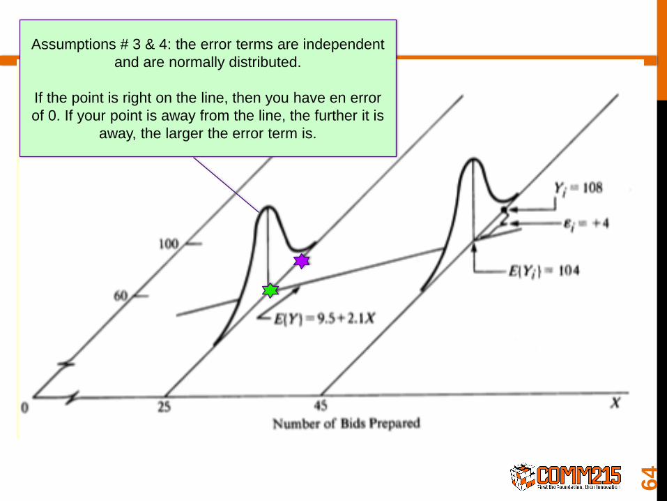
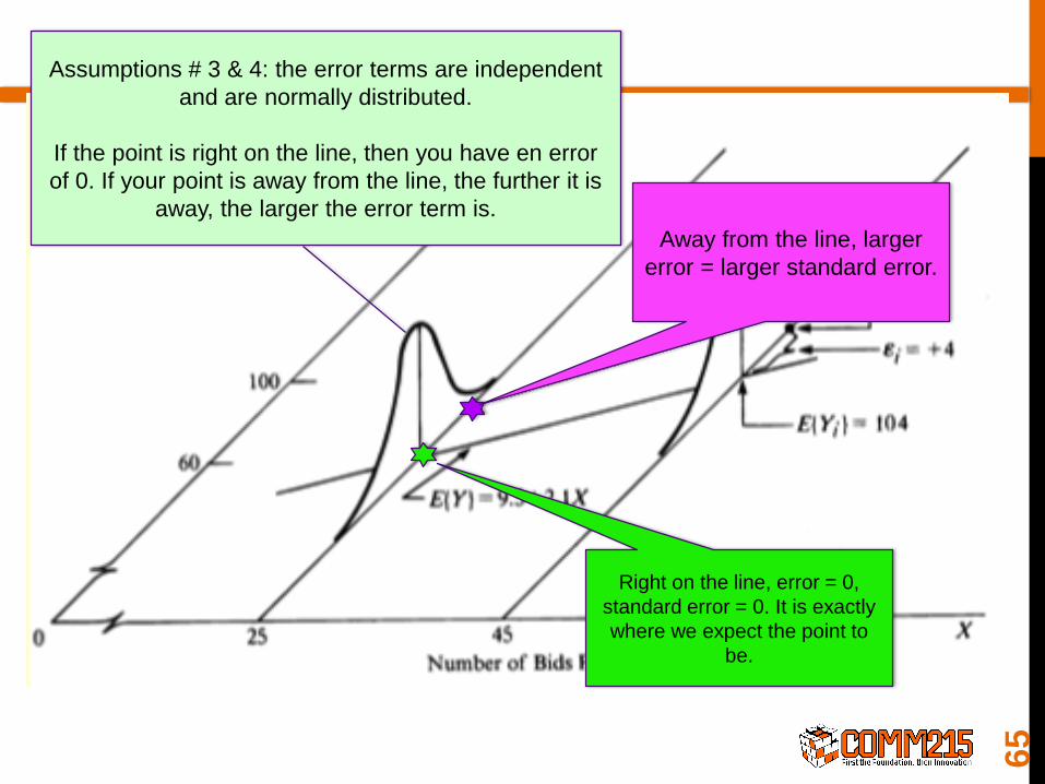
Assumptions # 3 & 4: the error terms are independent
and are normally distributed.
If the point is right on the line, then you have en error
of 0. If your point is away from the line, the further it is
away, the larger the error term is.
64
S.L.S.Ly
C215
Assumptions # 3 & 4: the error terms are independent
and are normally distributed.
If the point is right on the line, then you have en error
of 0. If your point is away from the line, the further it is
away, the larger the error term is.
Away from the line, larger
error = larger standard error.
Right on the line, error = 0,
standard error = 0. It is exactly
where we expect the point to
be.
65
S.L.S.Ly
C215
66
67
Testing for Significance
Covariance & Coefficient of Correlation
Using the Estimated Regression –Equation for Estimation and Prediction
S.L.S.Ly
C215
5. TESTING FOR SIGNIFICANCE
ESTIMATE σ2
TESTING FOR SIGNIFICANCE
CONFIDENCE INTERVAL FOR B1
68

S.L.S.Ly
C215
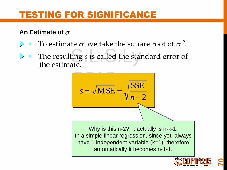
An Estimate of s 2
TESTING FOR SIGNIFICANCE
2
10
2 )()ˆ(SSE iiii xbbyyy
where:
s 2 = MSE = SSE/(n 2)
The mean square error (MSE) provides the estimate
of s 2, and the notation s2 is also used.
69
SSE =å yi2 -b0 yi -b1å xiyiå
Bowerman, et al. (2017) pp. 551
S.L.S.Ly
C215
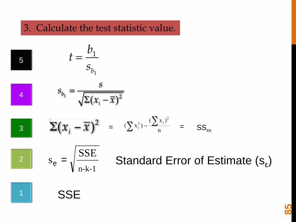
TESTING FOR SIGNIFICANCE
An Estimate of s
2
SSEMSE
ns
• To estimate s we take the square root of s 2.
• The resulting s is called the standard error ofthe estimate.
Why is this n-2?, it actually is n-k-1.
In a simple linear regression, since you always
have 1 independent variable (k=1), therefore
automatically it becomes n-1-1.
70

S.L.S.Ly
C215
STANDARD ERROR OF THE ESTIMATE
14-
71
Large Standard Error Small Standard Error

S.L.S.Ly
C215
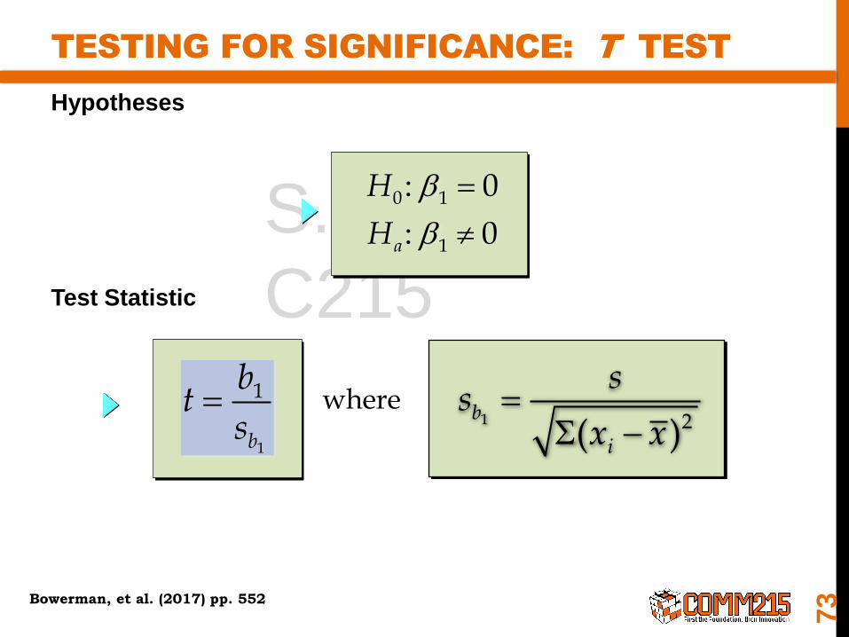
TESTING FOR SIGNIFICANCE
To test for a significant regression relationship, wemust conduct a hypothesis test to determine whetherthe value of b1 is zero.
Two tests are commonly used:
t Test and F Test
Both the t test and F test require an estimate of s 2,the variance of e in the regression model.
72
S.L.S.Ly
C215
TESTING FOR SIGNIFICANCE: T TEST
Hypotheses
Test Statistic
73
0 1: 0H b
1: 0aH b
1
1
b
bt
s where
1 2( )b
i
ss
x x
Bowerman, et al. (2017) pp. 552
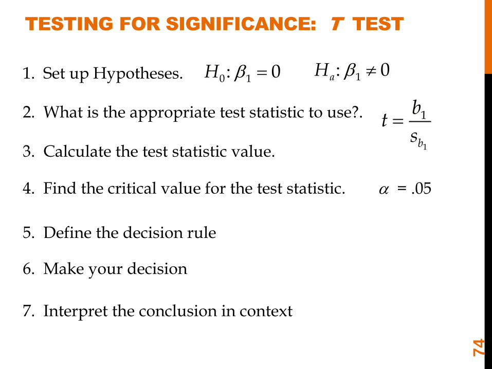
1. Set up Hypotheses.
2. What is the appropriate test statistic to use?.
3. Calculate the test statistic value.
a = .054. Find the critical value for the test statistic.
0 1: 0H b 1: 0aH b
1
1
b
bt
s
5. Define the decision rule
6. Make your decision
7. Interpret the conclusion in context
TESTING FOR SIGNIFICANCE: T TEST
74
S.L.S.Ly
C215
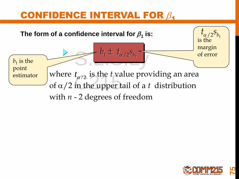
The form of a confidence interval for b1 is:
CONFIDENCE INTERVAL FOR b1
11 /2 bb t sa
where is the t value providing an area
of a/2 in the upper tail of a t distribution
with n - 2 degrees of freedom
2/at
b1 is thepointestimator
is themarginof error
1/2 bt sa
75
S.L.S.Ly
C215
CONFIDENCE INTERVAL FOR b1
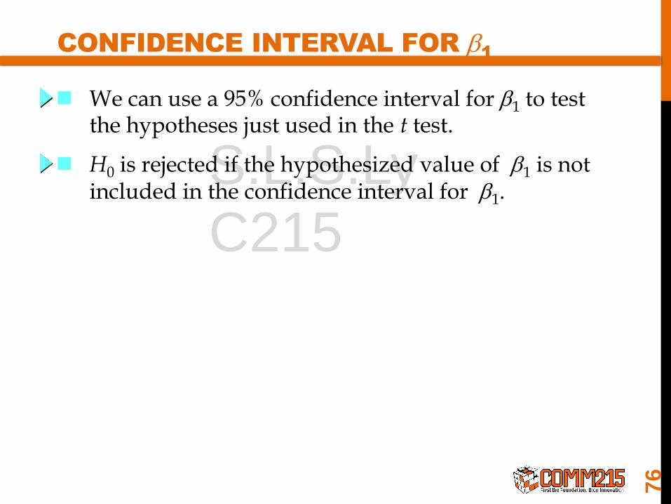
H0 is rejected if the hypothesized value of b1 is notincluded in the confidence interval for b1.
We can use a 95% confidence interval for b1 to testthe hypotheses just used in the t test.
76

S.L.S.Ly
C215
CONFIDENCE INTERVAL FOR b1
Reject H0 if 0 is not included in
the confidence interval for b1.
0 is not included in the confidence interval.
Reject H0
= 5.0 ± 2.048(2.25) = 5.0 ± 4.60812/1 bstb a
or 0.392 to 9.608
Rejection Rule
95% Confidence Interval for b1
Conclusion
77

S.L.S.Ly
C215
SOME CAUTIONS ABOUT THE
INTERPRETATION OF SIGNIFICANCE TESTS
Just because we are able to reject H0: b1 = 0 anddemonstrate statistical significance does not enableus to conclude that there is a linear relationshipbetween x and y.
Rejecting H0: b1 = 0 and concluding that therelationship between x and y is significant does not enable us to conclude that a cause-and-effectrelationship is present between x and y.
78

S.L.S.Ly
C215
7 SECTIONS
1. SIMPLE LINEAR REGRESSION MODEL 14.2
2. LEAST SQUARE METHOD 14.2
3. COEFFICIENT OF DETERMINATION 14.2
4. MODEL ASSUMPTIONS 14.2
5. TESTING FOR SIGNIFICANCE 14.3
6. COVARIANCE & COEFFICIENT OF
CORRELATION 14.1
7. USING THE ESTIMATED REGRESSION 11.7
EQUATION FOR ESTIMATION AND PREDICTION
S.L.S.Ly
C215
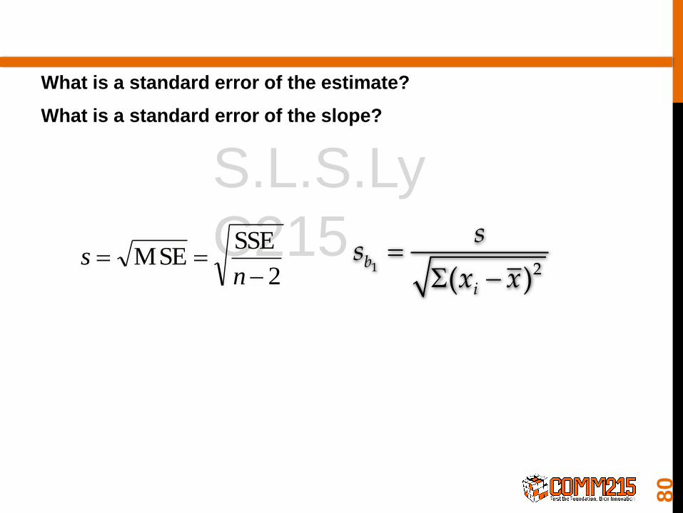
What is a standard error of the estimate?
What is a standard error of the slope?
2
SSEMSE
ns
1 2( )b
i
ss
x x
80
S.L.S.Ly
C215
PROBLEM # 10.15
At 5% level significance. The manager of Colonial Furniture has been reviewing weekly advertising expenditures. During the past 6 months, all advertisements for the store have appeared in the local newspaper. The number of ads per week has varied from one to seven. The store’s sales staff has been tracking the number of customers who enter the store each week. The number of ads and the number of customers per week for the past 26 weeks were recorded.
a. Determine the sample regression line
b. Interpret the coefficients.
c. Can the manager infer that the larger the number of ads, the larger the number of customers?
d. Find and interpret the coefficient of determination.
e. In your opinion, is it worthwhile exercise to use the regression equation to predict the number of customers who will enter the store, given that Colonial intends to advertise five times in the newspaper? If so, find the 95% prediction interval. If not, explain why not.
81
S.L.S.Ly
C215
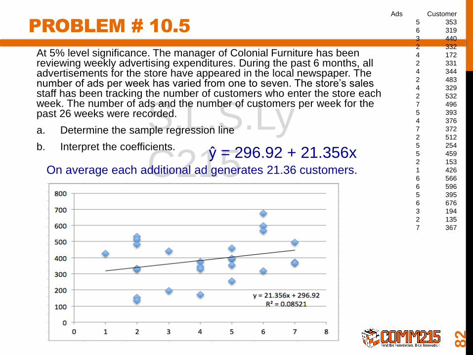
PROBLEM # 10.5
At 5% level significance. The manager of Colonial Furniture has been reviewing weekly advertising expenditures. During the past 6 months, all advertisements for the store have appeared in the local newspaper. The number of ads per week has varied from one to seven. The store’s sales staff has been tracking the number of customers who enter the store each week. The number of ads and the number of customers per week for the past 26 weeks were recorded.
a. Determine the sample regression line
b. Interpret the coefficients.
82
Ads Customer
5 353
6 319
3 440
2 332
4 172
2 331
4 344
2 483
4 329
2 532
7 496
5 393
4 376
7 372
2 512
5 254
5 459
2 153
1 426
6 566
6 596
5 395
6 676
3 194
2 135
7 367
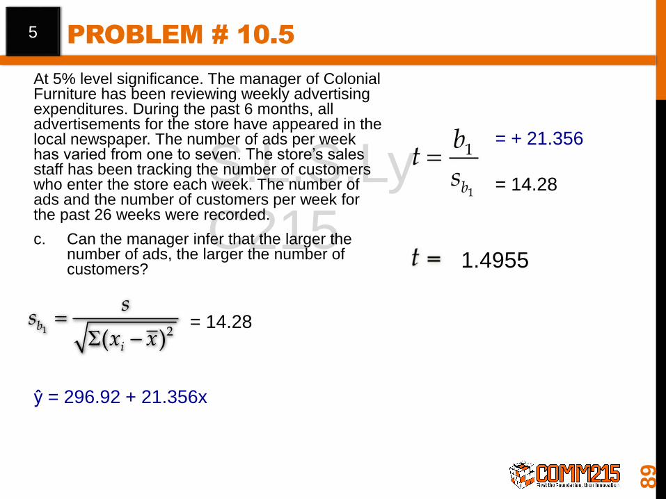
ŷ = 296.92 + 21.356xOn average each additional ad generates 21.36 customers.
S.L.S.Ly
C215
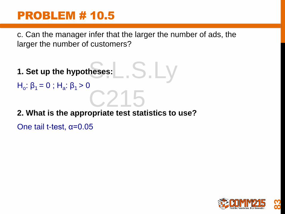
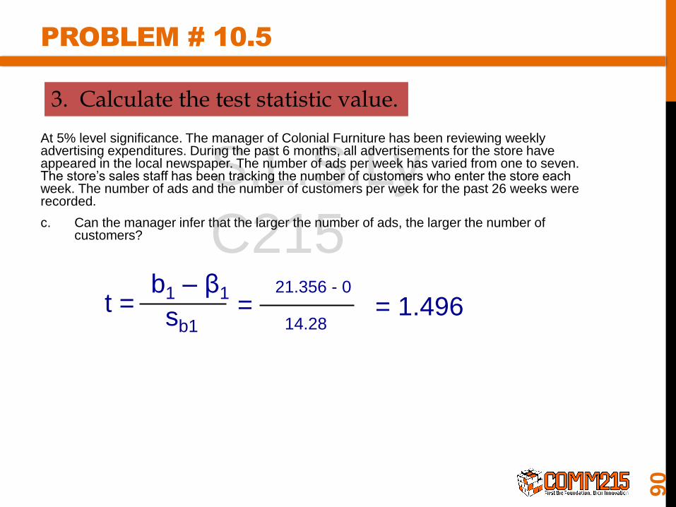
PROBLEM # 10.5
c. Can the manager infer that the larger the number of ads, the
larger the number of customers?
1. Set up the hypotheses:
Ho: β1 = 0 ; Ha: β1 > 0
2. What is the appropriate test statistics to use?
One tail t-test, α=0.05
83
1. Set up Hypotheses.
2. What is the appropriate test statistic to use?.
3. Calculate the test statistic value.
a = .054. Find the critical value for the test statistic.
Testing for Significance: t Test
1
1
b
bt
s
5. Define the decision rule
6. Make your decision
7. Interpret the conclusion in context
84
3. Calculate the test statistic value.
1
1
b
bt
s
2n
SSEs
-=e
1
3
2
4
5
SSE
Standard Error of Estimate (sε)
= = SSxx
1 2( )b
i
ss
x x
n-k-1
85

S.L.S.Ly
C215
PROBLEM # 10.5
At 5% level significance. The manager of Colonial Furniture has been reviewing weekly advertising expenditures. During the past 6 months, all advertisements for the store have appeared in the local newspaper. The number of ads per week has varied from one to seven. The store’s sales staff has been tracking the number of customers who enter the store each week. The number of ads and the number of customers per week for the past 26 weeks were recorded.
c. Can the manager infer that the larger the number of ads, the larger the number of customers?
Ads x Customer y ŷ = 296.92 + 21.356x y-ŷ (y-ŷ)2
5.00 353.00 403.70 -50.70 2570.49
6.00 319.00 425.06 -106.06 11247.88
3.00 440.00 360.99 79.01 6242.90
2.00 332.00 339.63 -7.63 58.25
4.00 172.00 382.34 -210.34 44244.60
2.00 331.00 339.63 -8.63 74.51
4.00 344.00 382.34 -38.34 1470.26
2.00 483.00 339.63 143.37 20554.38
4.00 329.00 382.34 -53.34 2845.58
2.00 532.00 339.63 192.37 37005.45
7.00 496.00 446.41 49.59 2458.97
5.00 393.00 403.70 -10.70 114.49
4.00 376.00 382.34 -6.34 40.25
7.00 372.00 446.41 -74.41 5537.15
2.00 512.00 339.63 172.37 29710.73
5.00 254.00 403.70 -149.70 22410.09
5.00 459.00 403.70 55.30 3058.09
2.00 153.00 339.63 -186.63 34831.50
1.00 426.00 318.28 107.72 11604.46
6.00 566.00 425.06 140.94 19865.21
6.00 596.00 425.06 170.94 29221.85
5.00 395.00 403.70 -8.70 75.69
6.00 676.00 425.06 250.94 62972.89
3.00 194.00 360.99 -166.99 27884.99
2.00 135.00 339.63 -204.63 41874.26
7.00 367.00 446.41 -79.41 6306.27
424281.17
SSE = Σ(y-ŷ)2
1
SSE = Σ(y-ŷ)2 = 424281.17
86

S.L.S.Ly
C215
PROBLEM # 10.5
At 5% level significance. The manager of Colonial Furniture has been reviewing weekly advertising expenditures. During the past 6 months, all advertisements for the store have appeared in the local newspaper. The number of ads per week has varied from one to seven. The store’s sales staff has been tracking the number of customers who enter the store each week. The number of ads and the number of customers per week for the past 26 weeks were recorded.
c. Can the manager infer that the larger the number of ads, the larger the number of customers?
2
2n
SSEs
-=e
SSE = Σ(y-ŷ)2 = 424281.17
2n
SSEs
-=e
n-k-1
424281.17
26-1-1
2n
SSEs
-=e 132.96
87
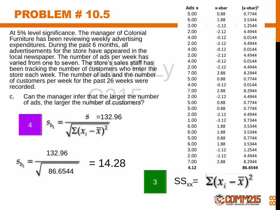
S.L.S.Ly
C215
PROBLEM # 10.5
At 5% level significance. The manager of Colonial Furniture has been reviewing weekly advertising expenditures. During the past 6 months, all advertisements for the store have appeared in the local newspaper. The number of ads per week has varied from one to seven. The store’s sales staff has been tracking the number of customers who enter the store each week. The number of ads and the number of customers per week for the past 26 weeks were recorded.
c. Can the manager infer that the larger the number of ads, the larger the number of customers?
SSxx=
Ads x x-xbar (x-xbar)2
5.00 0.88 0.7744
6.00 1.88 3.5344
3.00 -1.12 1.2544
2.00 -2.12 4.4944
4.00 -0.12 0.0144
2.00 -2.12 4.4944
4.00 -0.12 0.0144
2.00 -2.12 4.4944
4.00 -0.12 0.0144
2.00 -2.12 4.4944
7.00 2.88 8.2944
5.00 0.88 0.7744
4.00 -0.12 0.0144
7.00 2.88 8.2944
2.00 -2.12 4.4944
5.00 0.88 0.7744
5.00 0.88 0.7744
2.00 -2.12 4.4944
1.00 -3.12 9.7344
6.00 1.88 3.5344
6.00 1.88 3.5344
5.00 0.88 0.7744
6.00 1.88 3.5344
3.00 -1.12 1.2544
2.00 -2.12 4.4944
7.00 2.88 8.2944
4.12 86.6544
3
1 2( )b
i
ss
x x
=132.96
1 2( )b
i
ss
x x
86.6544
132.96
= 14.28
4
88
S.L.S.Ly
C215
PROBLEM # 10.5
At 5% level significance. The manager of Colonial Furniture has been reviewing weekly advertising expenditures. During the past 6 months, all advertisements for the store have appeared in the local newspaper. The number of ads per week has varied from one to seven. The store’s sales staff has been tracking the number of customers who enter the store each week. The number of ads and the number of customers per week for the past 26 weeks were recorded.
c. Can the manager infer that the larger the number of ads, the larger the number of customers?
5
1
1
b
bt
s
1 2( )b
i
ss
x x
= 14.28
ŷ = 296.92 + 21.356x
= + 21.356
= 14.28
1.4955
89
S.L.S.Ly
C215
PROBLEM # 10.5
At 5% level significance. The manager of Colonial Furniture has been reviewing weekly advertising expenditures. During the past 6 months, all advertisements for the store have appeared in the local newspaper. The number of ads per week has varied from one to seven. The store’s sales staff has been tracking the number of customers who enter the store each week. The number of ads and the number of customers per week for the past 26 weeks were recorded.
c. Can the manager infer that the larger the number of ads, the larger the number of customers?
3. Calculate the test statistic value.
t = b1 – β1
sb1=
21.356 - 0
14.28= 1.496
90

S.L.S.Ly
C215
PROBLEM # 10.5
4. Find the critical value of the test statistics
tα, n-k-1= t0.05,24 = 1.711
5. Define the decision rule
Reject Ho, if tobserved > tcritical, otherwise do not reject.
6. Make your decision
Since tobserved= 1.4955 < tcritical , then we do not reject Ho
7. Interpret in the context
There is not enough evidence to conclude that the larger the number of ads the larger the number of customers.
91
92
Covariance & Coefficient of Correlation
Using the Estimated Regression –Equation for Estimation and Prediction

S.L.S.Ly
C215
6. COVARIANCE &
COEFFICIENT OF CORRELATION
Covariance
Interpretation of the covariance
Correlation coefficient
93

S.L.S.Ly
C215
MEASURES OF ASSOCIATION
BETWEEN TWO VARIABLES
94
Thus far we have examined numerical methods usedto summarize the data for one variable at a time.
Often a manager or decision maker is interested inthe relationship between two variables.
Two descriptive measures of the relationship between two variables are covariance and correlationcoefficient.

S.L.S.Ly
C215
2 VARIABLE RELATIONSHIPS
S.L.S.Ly
C215
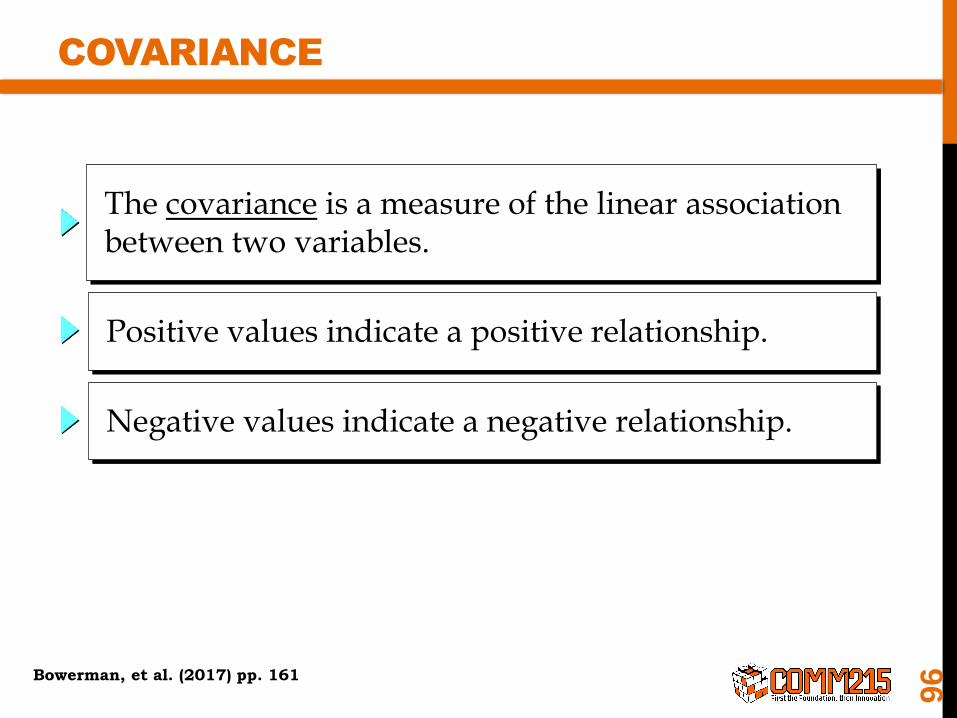
COVARIANCE
96
Positive values indicate a positive relationship.
Negative values indicate a negative relationship.
The covariance is a measure of the linear associationbetween two variables.
Bowerman, et al. (2017) pp. 161

The covariance is computed as follows:
forsamples
forpopulations
sx x y y
nxy
i i
( )( )
1
s
xyi x i yx y
N
( )( )
COVARIANCE
97

Just because two variables are highly correlated, it does not mean that one variable is the cause of theother.
Correlation is a measure of linear association and notnecessarily causation.
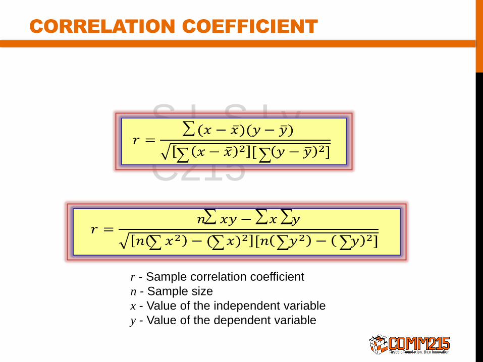
CORRELATION COEFFICIENT
98

The correlation coefficient is computed as follows:
forsamples
forpopulations
rs
s sxy
xy
x y
s
s sxy
xy
x y
CORRELATION COEFFICIENT
Pearson Product Moment
Correlation Coefficient.
99
S.L.S.Ly
C215
r - Sample correlation coefficient
n - Sample size
x - Value of the independent variable
y - Value of the dependent variable
CORRELATION COEFFICIENT
S.L.S.Ly
C215
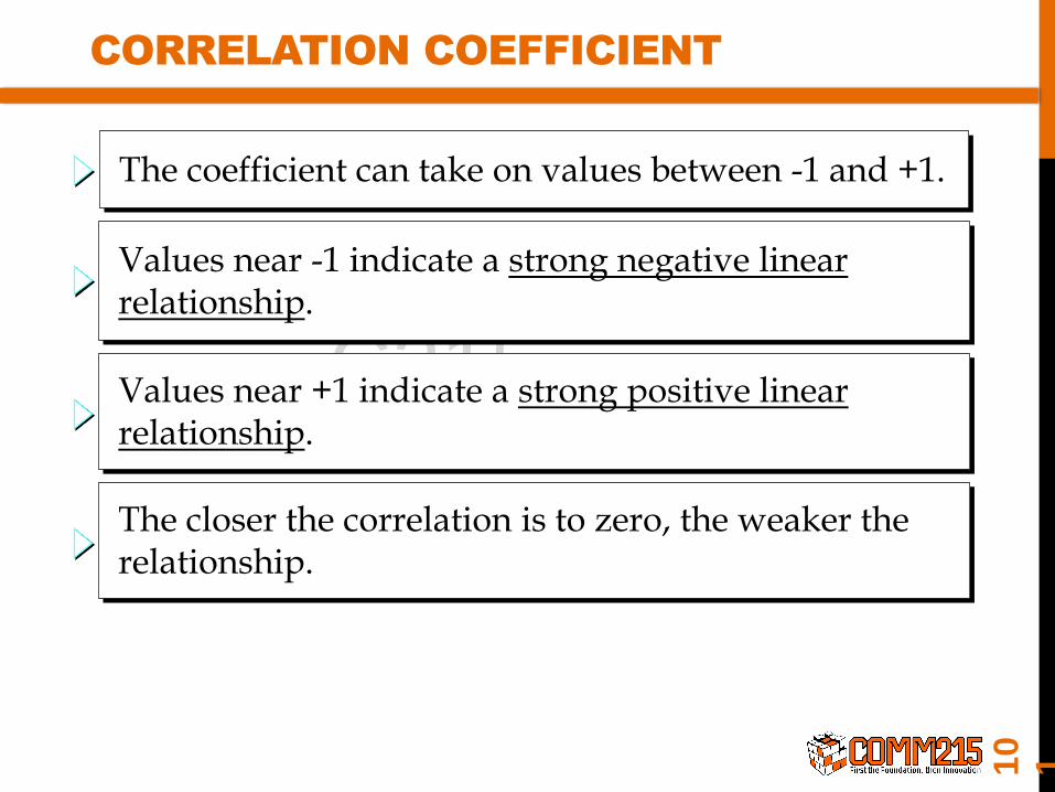
CORRELATION COEFFICIENT
Values near +1 indicate a strong positive linearrelationship.
Values near -1 indicate a strong negative linearrelationship.
The coefficient can take on values between -1 and +1.
The closer the correlation is to zero, the weaker therelationship.
10
1

Covariance and Correlation Coefficient
277.6
259.5
269.1
267.0
255.6
272.9
69
71
70
70
71
69
x y
10.65
-7.45
2.15
0.05
-11.35
5.95
-1.0
1.0
0
0
1.0
-1.0
-10.65
-7.45
0
0
-11.35
-5.95
( )ix x ( )( )i ix x y y ( )iy y
Average
Std. Dev.
267.0 70.0 -35.40
8.2192 .8944
Total
102
S.L.S.Ly
C215
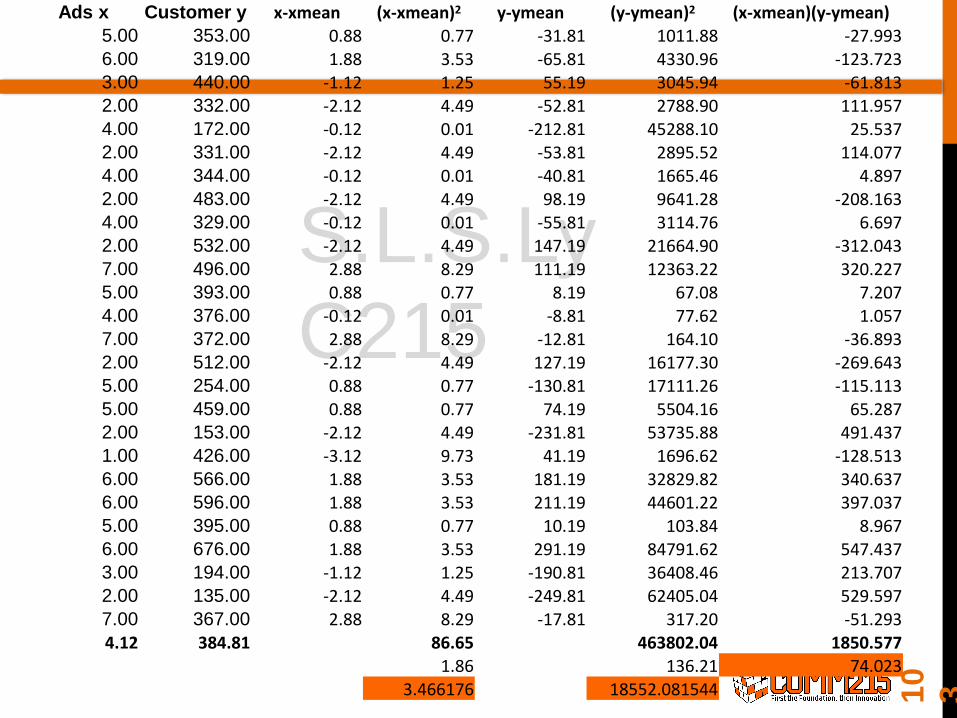
Ads x Customer y x-xmean (x-xmean)2 y-ymean (y-ymean)2 (x-xmean)(y-ymean)5.00 353.00 0.88 0.77 -31.81 1011.88 -27.9936.00 319.00 1.88 3.53 -65.81 4330.96 -123.7233.00 440.00 -1.12 1.25 55.19 3045.94 -61.8132.00 332.00 -2.12 4.49 -52.81 2788.90 111.9574.00 172.00 -0.12 0.01 -212.81 45288.10 25.537
2.00 331.00 -2.12 4.49 -53.81 2895.52 114.0774.00 344.00 -0.12 0.01 -40.81 1665.46 4.8972.00 483.00 -2.12 4.49 98.19 9641.28 -208.163
4.00 329.00 -0.12 0.01 -55.81 3114.76 6.6972.00 532.00 -2.12 4.49 147.19 21664.90 -312.0437.00 496.00 2.88 8.29 111.19 12363.22 320.2275.00 393.00 0.88 0.77 8.19 67.08 7.2074.00 376.00 -0.12 0.01 -8.81 77.62 1.0577.00 372.00 2.88 8.29 -12.81 164.10 -36.893
2.00 512.00 -2.12 4.49 127.19 16177.30 -269.6435.00 254.00 0.88 0.77 -130.81 17111.26 -115.1135.00 459.00 0.88 0.77 74.19 5504.16 65.2872.00 153.00 -2.12 4.49 -231.81 53735.88 491.4371.00 426.00 -3.12 9.73 41.19 1696.62 -128.5136.00 566.00 1.88 3.53 181.19 32829.82 340.6376.00 596.00 1.88 3.53 211.19 44601.22 397.0375.00 395.00 0.88 0.77 10.19 103.84 8.967
6.00 676.00 1.88 3.53 291.19 84791.62 547.437
3.00 194.00 -1.12 1.25 -190.81 36408.46 213.7072.00 135.00 -2.12 4.49 -249.81 62405.04 529.5977.00 367.00 2.88 8.29 -17.81 317.20 -51.2934.12 384.81 86.65 463802.04 1850.577
1.86 136.21 74.0233.466176 18552.081544 1
0
3

S.L.S.Ly
C215
Ads x Customer yx-xmean (x-xmean)2 y-ymean (y-ymean)2
(x-xmean)(y-ymean)
5.00 353.00 0.88 0.77 -31.81 1011.88 -27.993… …. … … … … …
6.00 566.00 1.88 3.53 181.19 32829.82 340.6376.00 596.00 1.88 3.53 211.19 44601.22 397.0375.00 395.00 0.88 0.77 10.19 103.84 8.9676.00 676.00 1.88 3.53 291.19 84791.62 547.4373.00 194.00 -1.12 1.25 -190.81 36408.46 213.7072.00 135.00 -2.12 4.49 -249.81 62405.04 529.5977.00 367.00 2.88 8.29 -17.81 317.20 -51.2934.12 384.81 86.65 463802.04 1850.577
1.86 136.21 74.023
10
4

S.L.S.Ly
C215
Ads x Customer y x-xmean (x-xmean)2 y-ymean (y-ymean)2 (x-xmean)(y-ymean)5.00 353.00 0.88 0.77 -31.81 1011.88 -27.9936.00 319.00 1.88 3.53 -65.81 4330.96 -123.723
3.00 440.00 -1.12 1.25 55.19 3045.94 -61.8132.00 332.00 -2.12 4.49 -52.81 2788.90 111.9574.00 172.00 -0.12 0.01 -212.81 45288.10 25.5372.00 331.00 -2.12 4.49 -53.81 2895.52 114.0774.00 344.00 -0.12 0.01 -40.81 1665.46 4.8972.00 483.00 -2.12 4.49 98.19 9641.28 -208.163
4.00 329.00 -0.12 0.01 -55.81 3114.76 6.6972.00 532.00 -2.12 4.49 147.19 21664.90 -312.043
7.00 496.00 2.88 8.29 111.19 12363.22 320.2275.00 393.00 0.88 0.77 8.19 67.08 7.2074.00 376.00 -0.12 0.01 -8.81 77.62 1.0577.00 372.00 2.88 8.29 -12.81 164.10 -36.893
2.00 512.00 -2.12 4.49 127.19 16177.30 -269.6435.00 254.00 0.88 0.77 -130.81 17111.26 -115.1135.00 459.00 0.88 0.77 74.19 5504.16 65.287
2.00 153.00 -2.12 4.49 -231.81 53735.88 491.437
1.00 426.00 -3.12 9.73 41.19 1696.62 -128.5136.00 566.00 1.88 3.53 181.19 32829.82 340.6376.00 596.00 1.88 3.53 211.19 44601.22 397.037
5.00 395.00 0.88 0.77 10.19 103.84 8.9676.00 676.00 1.88 3.53 291.19 84791.62 547.4373.00 194.00 -1.12 1.25 -190.81 36408.46 213.7072.00 135.00 -2.12 4.49 -249.81 62405.04 529.5977.00 367.00 2.88 8.29 -17.81 317.20 -51.293
4.12 384.81 86.65 463802.04 1850.577
1.86 136.21 74.023
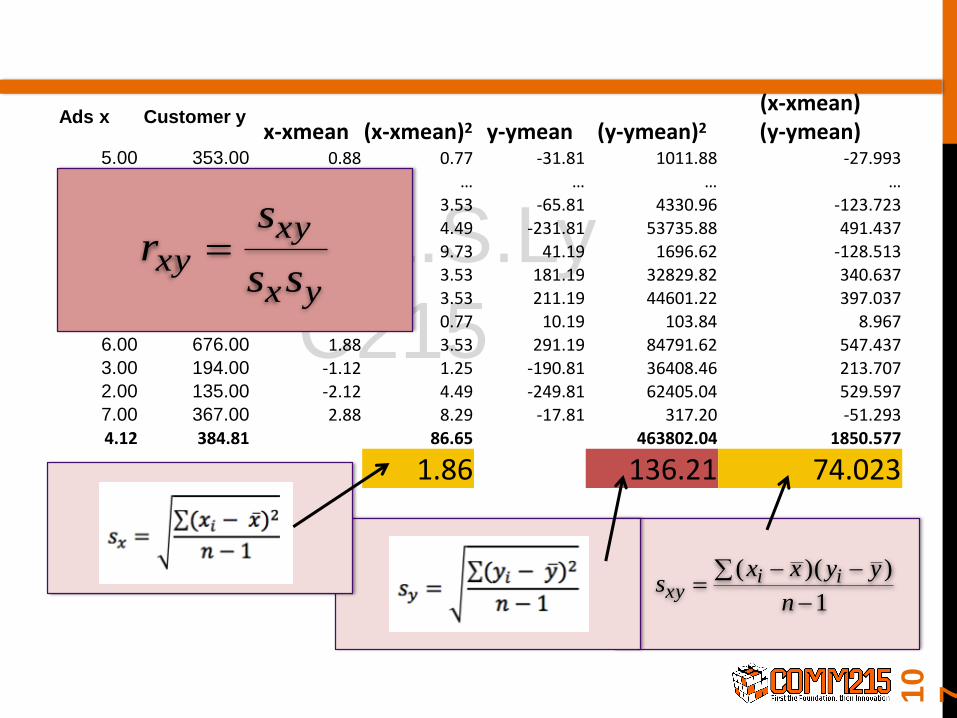
sx x y y
nxy
i i
( )( )
1
rs
s sxy
xy
x y
10
5

S.L.S.Ly
C215
PROBLEM # 10.5
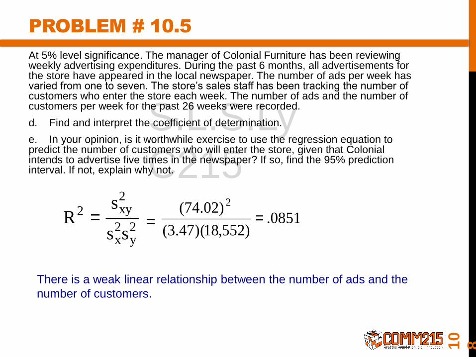
At 5% level significance. The manager of Colonial Furniture has been reviewing weekly advertising expenditures. During the past 6 months, all advertisements for the store have appeared in the local newspaper. The number of ads per week has varied from one to seven. The store’s sales staff has been tracking the number of customers who enter the store each week. The number of ads and the number of customers per week for the past 26 weeks were recorded.
d. Find and interpret the coefficient of determination.
e. In your opinion, is it worthwhile exercise to use the regression equation to predict the number of customers who will enter the store, given that Colonial intends to advertise five times in the newspaper? If so, find the 95% prediction interval. If not, explain why not.
10
6
S.L.S.Ly
C215
Ads x Customer yx-xmean (x-xmean)2 y-ymean (y-ymean)2
(x-xmean)(y-ymean)
5.00 353.00 0.88 0.77 -31.81 1011.88 -27.993… … … … … … …
6.00 319.00 1.88 3.53 -65.81 4330.96 -123.723
2.00 153.00 -2.12 4.49 -231.81 53735.88 491.4371.00 426.00 -3.12 9.73 41.19 1696.62 -128.5136.00 566.00 1.88 3.53 181.19 32829.82 340.637
6.00 596.00 1.88 3.53 211.19 44601.22 397.0375.00 395.00 0.88 0.77 10.19 103.84 8.9676.00 676.00 1.88 3.53 291.19 84791.62 547.4373.00 194.00 -1.12 1.25 -190.81 36408.46 213.7072.00 135.00 -2.12 4.49 -249.81 62405.04 529.5977.00 367.00 2.88 8.29 -17.81 317.20 -51.293
4.12 384.81 86.65 463802.04 1850.577
1.86 136.21 74.023
sx x y y
nxy
i i
( )( )
1
rs
s sxy
xy
x y
10
7
S.L.S.Ly
C215
PROBLEM # 10.5
At 5% level significance. The manager of Colonial Furniture has been reviewing weekly advertising expenditures. During the past 6 months, all advertisements for the store have appeared in the local newspaper. The number of ads per week has varied from one to seven. The store’s sales staff has been tracking the number of customers who enter the store each week. The number of ads and the number of customers per week for the past 26 weeks were recorded.
d. Find and interpret the coefficient of determination.
e. In your opinion, is it worthwhile exercise to use the regression equation to predict the number of customers who will enter the store, given that Colonial intends to advertise five times in the newspaper? If so, find the 95% prediction interval. If not, explain why not.
2y
2x
2xy2
ss
sR = 0851.
)552,18)(47.3(
)02.74( 2
=
There is a weak linear relationship between the number of ads and the
number of customers.
=
10
8
S.L.S.Ly
C215
PROBLEM # 10.5
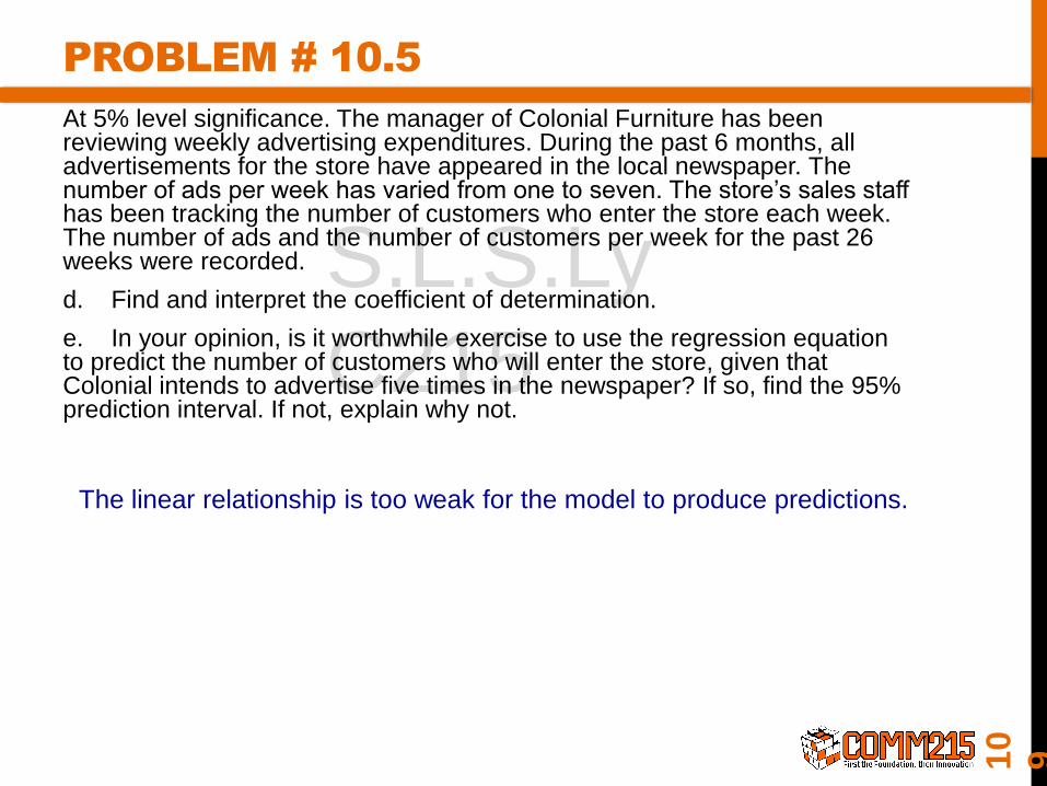
At 5% level significance. The manager of Colonial Furniture has been reviewing weekly advertising expenditures. During the past 6 months, all advertisements for the store have appeared in the local newspaper. The number of ads per week has varied from one to seven. The store’s sales staff has been tracking the number of customers who enter the store each week. The number of ads and the number of customers per week for the past 26 weeks were recorded.
d. Find and interpret the coefficient of determination.
e. In your opinion, is it worthwhile exercise to use the regression equation to predict the number of customers who will enter the store, given that Colonial intends to advertise five times in the newspaper? If so, find the 95% prediction interval. If not, explain why not.
The linear relationship is too weak for the model to produce predictions.
10
9
11
0
Using the Estimated Regression –Equation for Estimation and Prediction
S.L.S.Ly
C215
7. ESTIMATION
POINT ESTIMATION
INTERVAL ESTIMATION
CONFIDENCE INTERVAL FOR THE MEAN VALUE OF Y
PREDICTION INTERVAL FOR AN INDIVIDUAL VALUE OF Y
111

If 3 TV ads are run prior to a sale, we expect
the mean number of cars sold to be:
y = 10 + 5(3) = 25 cars
POINT ESTIMATION
112
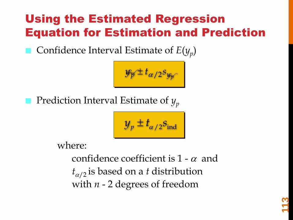
Using the Estimated Regression
Equation for Estimation and Prediction
/ y t sp yp
a 2
where:
confidence coefficient is 1 - a and
ta/2 is based on a t distribution
with n - 2 degrees of freedom
/2 indpy t sa
Confidence Interval Estimate of E(yp)
Prediction Interval Estimate of yp
113
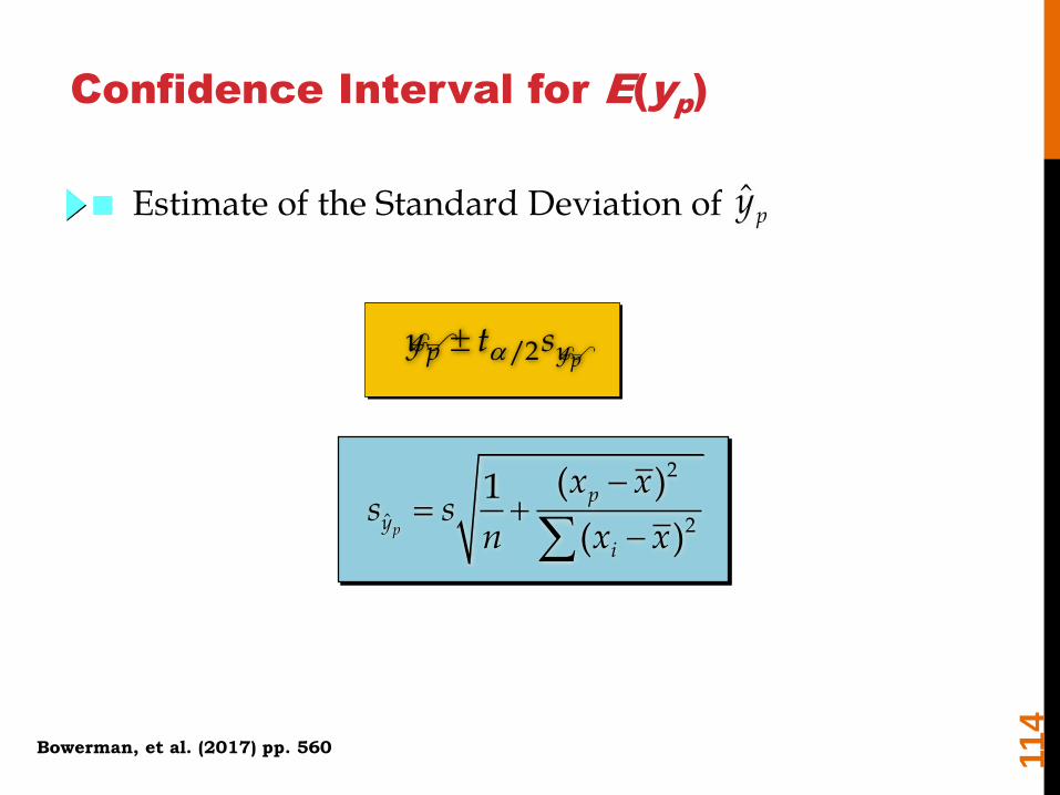
2
ˆ 2
( )1
( )p
p
y
i
x xs s
n x x
Estimate of the Standard Deviation of ˆ py
Confidence Interval for E(yp)
/ y t sp yp
a 2
114
Bowerman, et al. (2017) pp. 560

S.L.S.Ly
C215
CONFIDENCE VS PREDICTION INTERVAL
S.L.S.Ly
C215
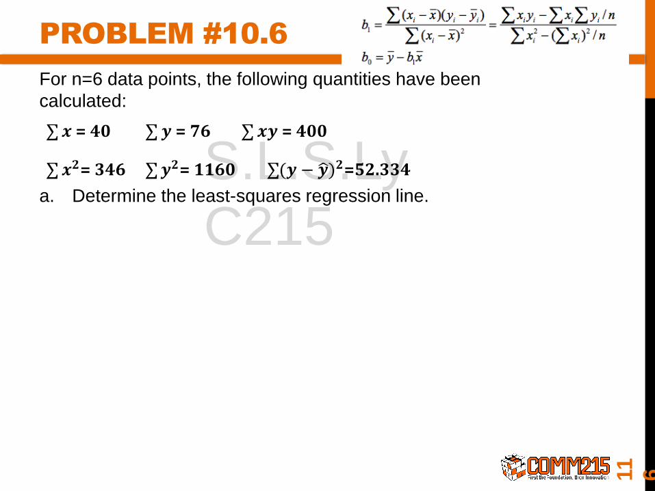
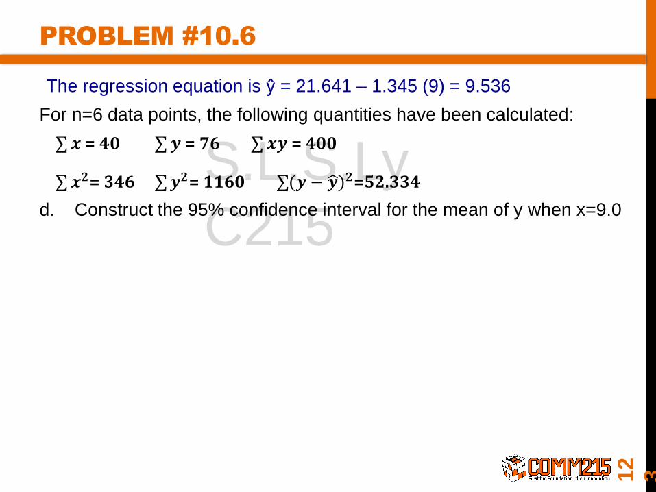
PROBLEM #10.6
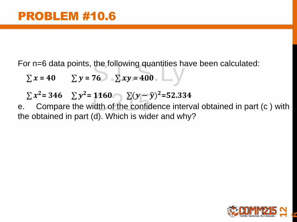
For n=6 data points, the following quantities have been
calculated:
a. Determine the least-squares regression line.
11
6

S.L.S.Ly
C215
PROBLEM #10.6
For n=6 data points, the following quantities have been
calculated:
a. Determine the least-squares regression line.
11
7
To determine the least squares regression line, we must calculate the slope
and y-intercept.
i i
1 2 22i
x y nxy 400 6(6.67)(12.67)b 1.354
346 6(6.67)x nx
- -= = = -
--
å
å
0 1b y b x 12.67 ( 1.354)(6.67) 21.701= - = - - =
400 – [(40)(76)/6]
346 – [(40)2/6]b1 -1.345
12.67 – (-1.345)(6.67) = 21.641
The regression equation is ŷ = 21.641 – 1.345 x
S.L.S.Ly
C215
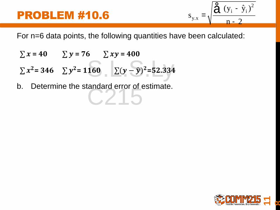
PROBLEM #10.6
For n=6 data points, the following quantities have been calculated:
b. Determine the standard error of estimate.
2i i
y.x
ˆ(y y ) 52.334s 3.617
n 2 6 2
-= = =
- -
å
11
8

S.L.S.Ly
C215
PROBLEM #10.6
For n=6 data points, the following quantities have been calculated:
b. Determine the standard error of estimate.
The standard error of the estimate is
2i i
y.x
ˆ(y y ) 52.334s 3.617
n 2 6 2
-= = =
- -
å
2i i
y.x
ˆ(y y ) 52.334s 3.617
n 2 6 2
-= = =
- -
å
11
9
S.L.S.Ly
C215
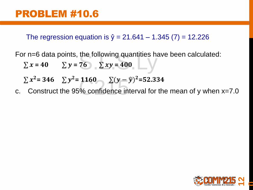
PROBLEM #10.6
For n=6 data points, the following quantities have been calculated:
c. Construct the 95% confidence interval for the mean of y when x=7.0
The regression equation is ŷ = 21.641 – 1.345 (7) = 12.226
12
0
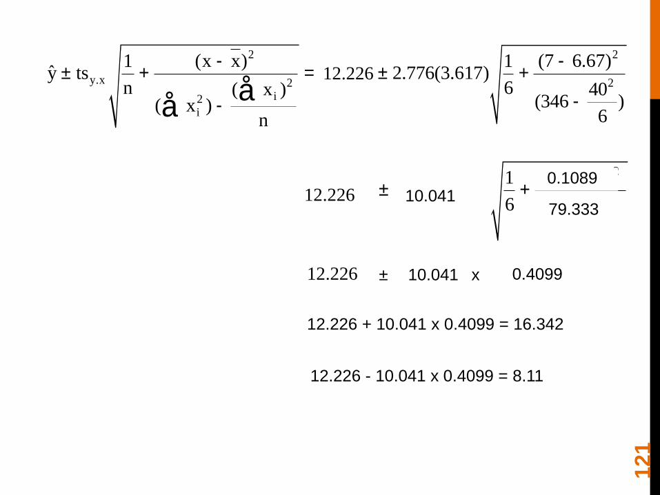
2 2
y.x 2 2i2
i
(x x) (7 6.67)1 1y ts 12.223 2.776(3.617)
n 6( x ) 40(346 )( x )
6n
12.223 4.116 (8.107, 16.339)
- -± + = ± +
--
= ± =
åå
12.226
2 2
y.x 2 2i2
i
(x x) (7 6.67)1 1y ts 12.223 2.776(3.617)
n 6( x ) 40(346 )( x )
6n
12.223 4.116 (8.107, 16.339)
- -± + = ± +
--
= ± =
åå
12.226
2 2
y.x 2 2i2
i
(x x) (7 6.67)1 1y ts 12.223 2.776(3.617)
n 6( x ) 40(346 )( x )
6n
12.223 4.116 (8.107, 16.339)
- -± + = ± +
--
= ± =
åå 79.333
0.1089
10.041 0.4099± x
12.226 + 10.041 x 0.4099 = 16.342
12.226 - 10.041 x 0.4099 = 8.11
12.226 10.041
121

S.L.S.Ly
C215
PROBLEM #10.6
For n=6 data points, the following quantities have been calculated:
c. Construct the 95% confidence interval for the mean of y when x=7.0
We also need the t-value with 6 - 2 = 4 degrees of freedom for a 95% interval;
this value is 2.776.
Therefore the 95% confidence interval for the mean value of y when x = 7 is:
2 2
y.x 2 2i2
i
(x x) (7 6.67)1 1y ts 12.223 2.776(3.617)
n 6( x ) 40(346 )( x )
6n
12.223 4.116 (8.107, 16.339)
- -± + = ± +
--
= ± =
åå
2 2
y.x 2 2i2
i
(x x) (7 6.67)1 1y ts 12.223 2.776(3.617)
n 6( x ) 40(346 )( x )
6n
12.223 4.116 (8.107, 16.339)
- -± + = ± +
--
= ± =
åå
The regression equation is ŷ = 21.641 – 1.345 (7) = 12.226
12.226
The confidence interval ranges from 8.110 to 16.342
12
2
S.L.S.Ly
C215
PROBLEM #10.6
For n=6 data points, the following quantities have been calculated:
d. Construct the 95% confidence interval for the mean of y when x=9.0
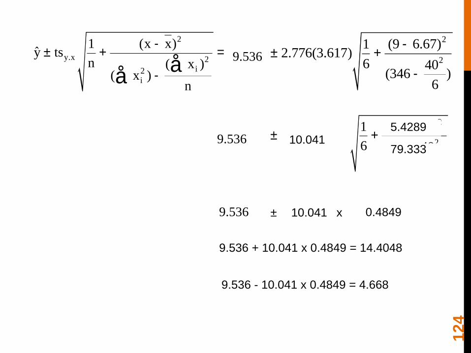
The regression equation is ŷ = 21.641 – 1.345 (9) = 9.536
12
3
2 2
y.x 2 2i2
i
(x x) (7 6.67)1 1y ts 12.223 2.776(3.617)
n 6( x ) 40(346 )( x )
6n
12.223 4.116 (8.107, 16.339)
- -± + = ± +
--
= ± =
åå
9.536
2 2
y.x 2 2i2
i
(x x) (7 6.67)1 1y ts 12.223 2.776(3.617)
n 6( x ) 40(346 )( x )
6n
12.223 4.116 (8.107, 16.339)
- -± + = ± +
--
= ± =
åå 79.333
5.4289
10.041 0.4849± x
9.536 + 10.041 x 0.4849 = 14.4048
9.536 - 10.041 x 0.4849 = 4.668
9.536 10.041
2 2
y.x 2 2i2
i
(x x) (9 6.67)1 1y ts 9.515 2.776(3.617)
n 6( x ) 40(346 )( x )
6n
9.515 4.868 (4.647, 14.383)
- -± + = ± +
--
= ± =
åå
9.536
124
S.L.S.Ly
C215
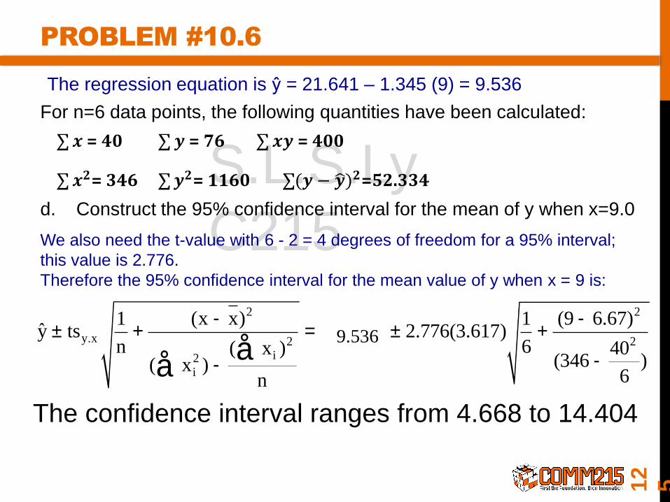
PROBLEM #10.6
For n=6 data points, the following quantities have been calculated:
d. Construct the 95% confidence interval for the mean of y when x=9.0
We also need the t-value with 6 - 2 = 4 degrees of freedom for a 95% interval;
this value is 2.776.
Therefore the 95% confidence interval for the mean value of y when x = 9 is:
2 2
y.x 2 2i2
i
(x x) (9 6.67)1 1y ts 9.515 2.776(3.617)
n 6( x ) 40(346 )( x )
6n
9.515 4.868 (4.647, 14.383)
- -± + = ± +
--
= ± =
åå
2 2
y.x 2 2i2
i
(x x) (9 6.67)1 1y ts 9.515 2.776(3.617)
n 6( x ) 40(346 )( x )
6n
9.515 4.868 (4.647, 14.383)
- -± + = ± +
--
= ± =
åå
The regression equation is ŷ = 21.641 – 1.345 (9) = 9.536
9.536
The confidence interval ranges from 4.668 to 14.404
12
5
S.L.S.Ly
C215
PROBLEM #10.6
For n=6 data points, the following quantities have been calculated:
e. Compare the width of the confidence interval obtained in part (c ) with
the obtained in part (d). Which is wider and why?
12
6

S.L.S.Ly
C215
PROBLEM #10.6
For n=6 data points, the following quantities have been calculated:
e. Compare the width of the confidence interval obtained in part (c ) with
the obtained in part (d). Which is wider and why?
The confidence interval in d is wider because 9 is farther
from the mean of x than 7.
For x = 7,
8.110 to 16.342
For x = 9,
4.668 to 14.404
12
7
2
ind 2
( )11
( )
p
i
x xs s
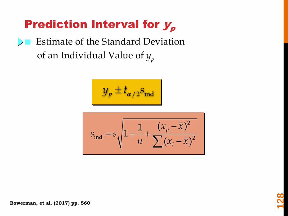
n x x
Estimate of the Standard Deviation
of an Individual Value of yp
Prediction Interval for yp
/2 indpy t sa
128
Bowerman, et al. (2017) pp. 560
S.L.S.Ly
C215
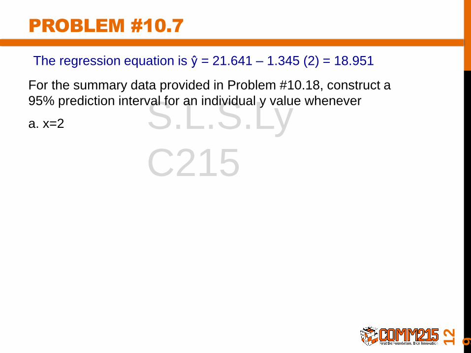
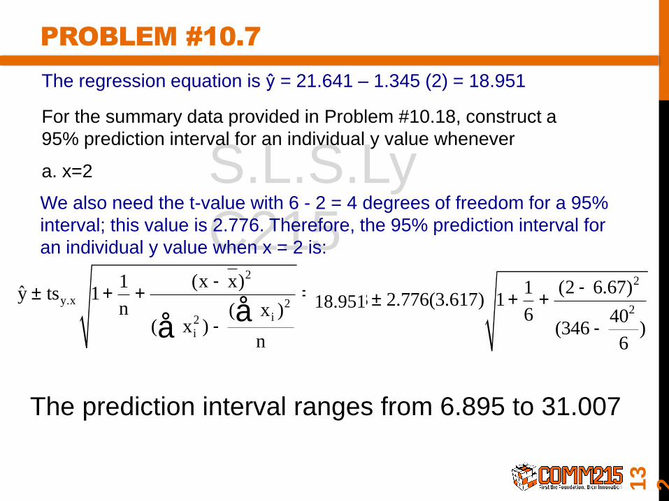
PROBLEM #10.7
For the summary data provided in Problem #10.18, construct a
95% prediction interval for an individual y value whenever
a. x=2
The regression equation is ŷ = 21.641 – 1.345 (2) = 18.951
12
9
S.L.S.Ly
C215
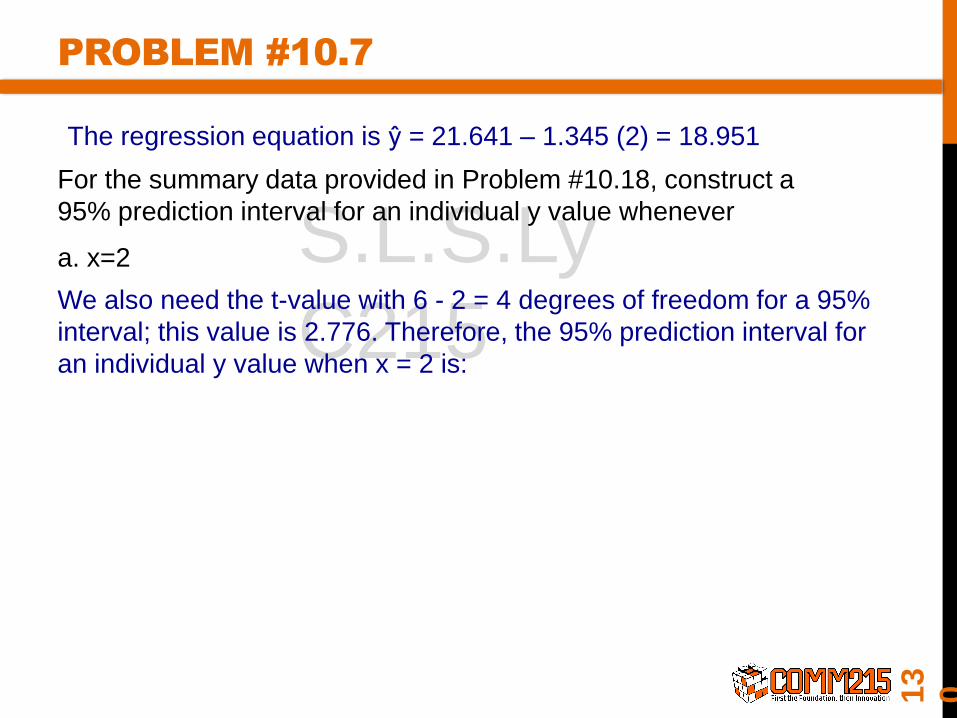
PROBLEM #10.7
For the summary data provided in Problem #10.18, construct a
95% prediction interval for an individual y value whenever
a. x=2
We also need the t-value with 6 - 2 = 4 degrees of freedom for a 95%
interval; this value is 2.776. Therefore, the 95% prediction interval for
an individual y value when x = 2 is:
The regression equation is ŷ = 21.641 – 1.345 (2) = 18.951
13
0
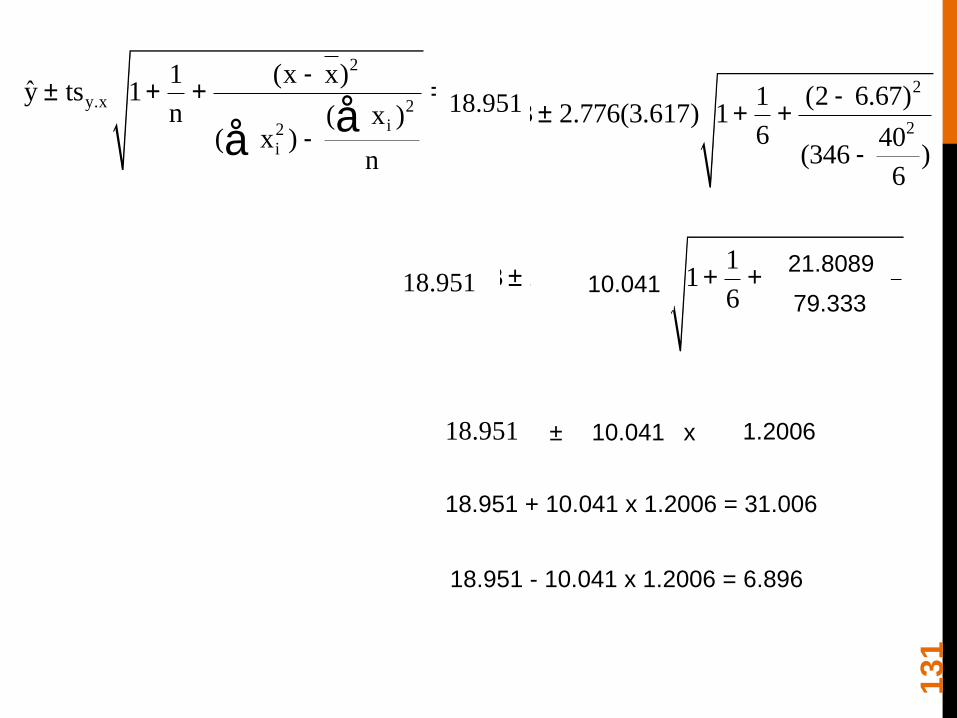
2 2
y.x 2 2i2
i
(x x) (2 6.67)1 1y ts 1 18.993 2.776(3.617) 1
n 6( x ) 40(346 )( x )
6n
18.993 12.056 (6.937, 31.049)
- -± + + = ± + +
--
= ± =
åå
18.951
79.333
21.8089
10.041 1.2006± x
18.951 + 10.041 x 1.2006 = 31.006
18.951 - 10.041 x 1.2006 = 6.896
18.951 10.041
2 2
y.x 2 2i2
i
(x x) (2 6.67)1 1y ts 1 18.993 2.776(3.617) 1
n 6( x ) 40(346 )( x )
6n
18.993 12.056 (6.937, 31.049)
- -± + + = ± + +
--
= ± =
åå
18.9512 2
y.x 2 2i2
i
(x x) (2 6.67)1 1y ts 1 18.993 2.776(3.617) 1
n 6( x ) 40(346 )( x )
6n
18.993 12.056 (6.937, 31.049)
- -± + + = ± + +
--
= ± =
åå
131
S.L.S.Ly
C215
PROBLEM #10.7
For the summary data provided in Problem #10.18, construct a
95% prediction interval for an individual y value whenever
a. x=2
We also need the t-value with 6 - 2 = 4 degrees of freedom for a 95%
interval; this value is 2.776. Therefore, the 95% prediction interval for
an individual y value when x = 2 is:
2 2
y.x 2 2i2
i
(x x) (2 6.67)1 1y ts 1 18.993 2.776(3.617) 1
n 6( x ) 40(346 )( x )
6n
18.993 12.056 (6.937, 31.049)
- -± + + = ± + +
--
= ± =
åå
The regression equation is ŷ = 21.641 – 1.345 (2) = 18.951
18.951
2 2
y.x 2 2i2
i
(x x) (2 6.67)1 1y ts 1 18.993 2.776(3.617) 1
n 6( x ) 40(346 )( x )
6n
18.993 12.056 (6.937, 31.049)
- -± + + = ± + +
--
= ± =
åå
The prediction interval ranges from 6.895 to 31.007
13
2


