CSE486, Penn StateRobert Collins
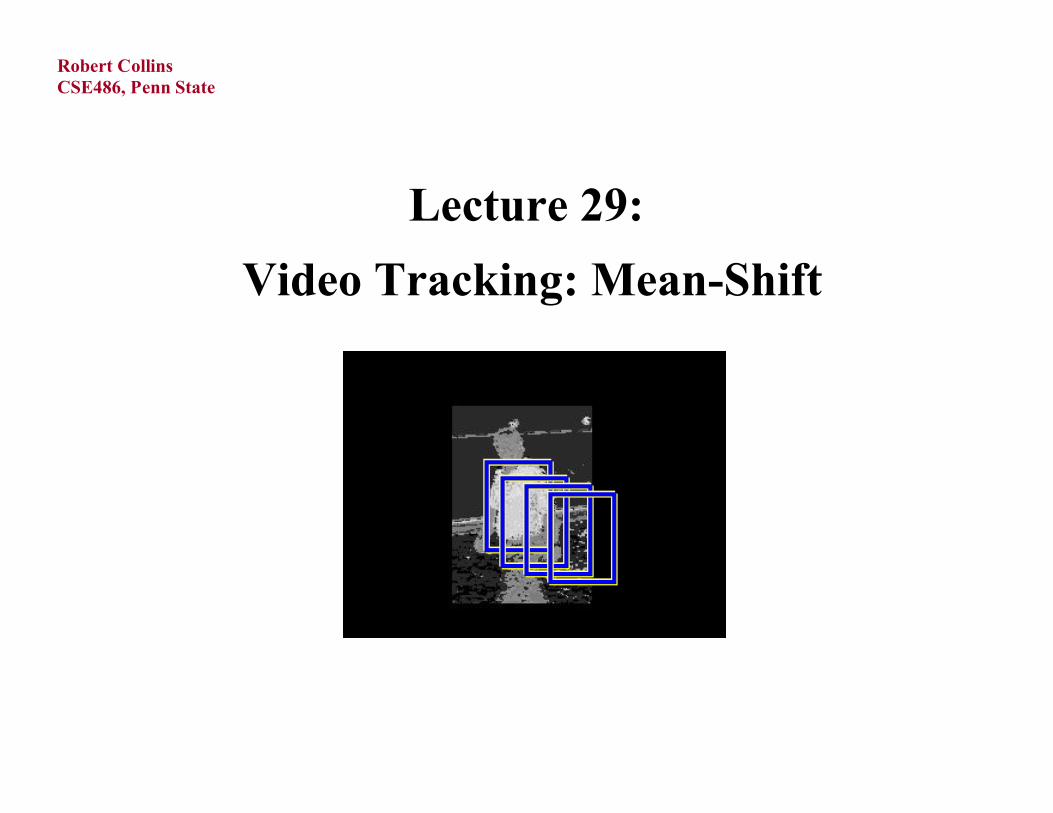
Lecture 29:
Video Tracking: Mean-Shift

CSE486, Penn StateRobert Collins
Appearance-Based Tracking
current frame +previous location
Mode-Seeking(e.g. mean-shift; Lucas-Kanade; particle filtering)
likelihood overobject location current location
appearance model(e.g. image template, or
color; intensity; edge histograms)

CSE486, Penn StateRobert Collins
Histogram Appearance Models
• Motivation – to track non-rigid objects, (like a walking person), it is hard to specifyan explicit 2D parametric motion model.
• Appearances of non-rigid objects can sometimes be modeled with color distributions

CSE486, Penn StateRobert Collins
Appearance via Color Histograms
Color distribution (1D histogram normalized to have unit weight)
R’
G’B’
discretize
R’ = R << (8 - nbits)G’ = G << (8 - nbits)B’ = B << (8-nbits)
Total histogram size is (2^(8-nbits))^3
example, 4-bit encoding of R,G and B channelsyields a histogram of size 16*16*16 = 4096.

CSE486, Penn StateRobert Collins
Smaller Color Histograms
R’G’
B’
discretize
R’ = R << (8 - nbits)G’ = G << (8 - nbits)B’ = B << (8-nbits)
Total histogram size is 3*(2^(8-nbits))
example, 4-bit encoding of R,G and B channelsyields a histogram of size 3*16 = 48.
Histogram information can be much much smaller if we are willing to accept a loss in color resolvability.
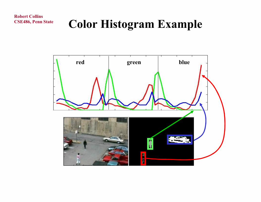
Marginal R distribution
Marginal G distribution
Marginal B distribution
CSE486, Penn StateRobert Collins
Color Histogram Example
red green blue

CSE486, Penn StateRobert Collins
Normalized Color
(r,g,b) (r’,g’,b’) = (r,g,b) / (r+g+b)
Normalized color divides out pixel luminance (brightness), leaving behind only chromaticity (color) information. The result is less sensitive to variations due to illumination/shading.
CSE486, Penn StateRobert Collins
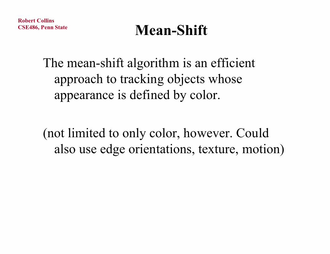
Mean-Shift
The mean-shift algorithm is an efficient approach to tracking objects whose appearance is defined by color.
(not limited to only color, however. Could also use edge orientations, texture, motion)

CSE486, Penn StateRobert Collins
What is Mean Shift ?
Non-parametricDensity Estimation
Non-parametricDensity GRADIENT Estimation
(Mean Shift)
Data
Discrete PDF Representation
PDF Analysis
A tool for:Finding modes in a set of data samples, manifesting an underlying probability density function (PDF) in RN
Ukrainitz&Sarel, Weizmann
PDF in feature space• Color space• Scale space• Actually any feature space you can conceive• …

CSE486, Penn StateRobert Collins
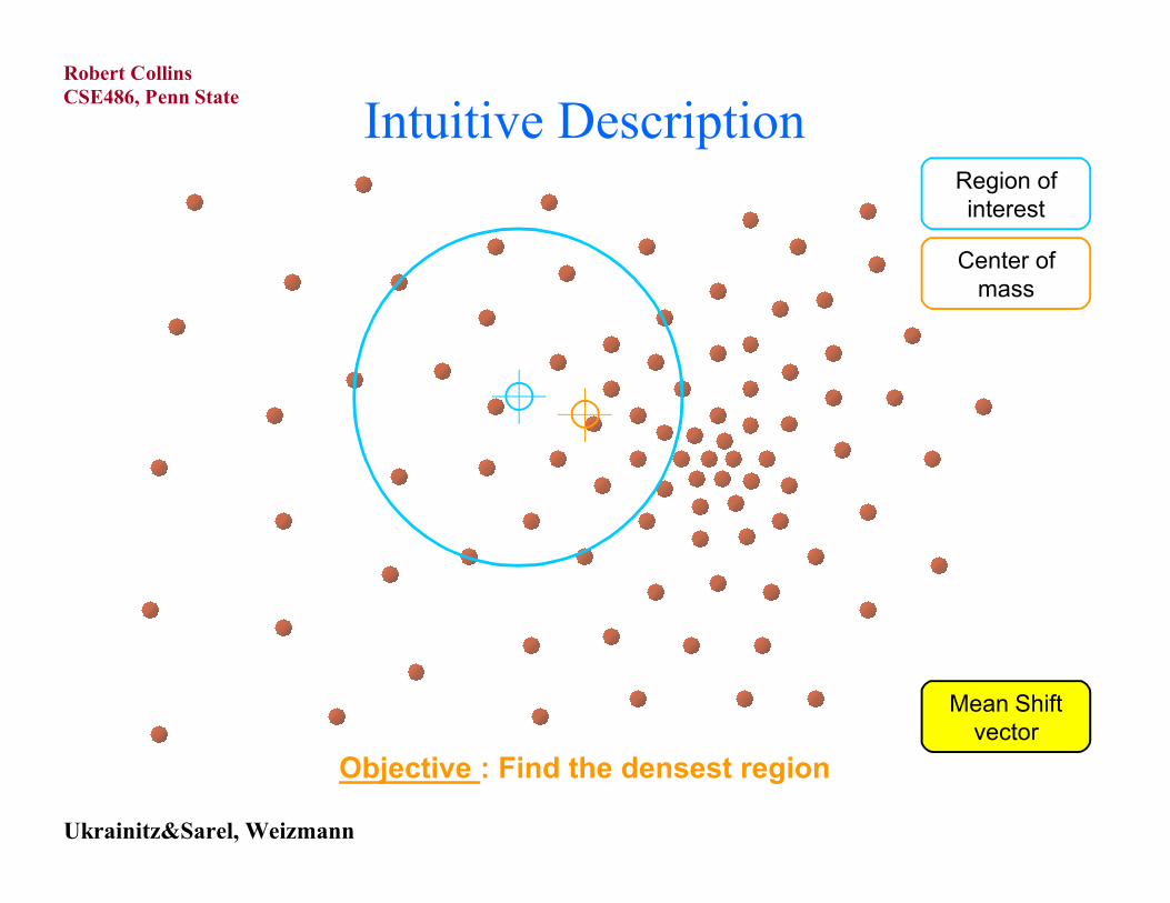
Intuitive Description
Distribution of identical billiard balls
Region ofinterest
Center ofmass
Mean Shiftvector
Objective : Find the densest region
Ukrainitz&Sarel, Weizmann
CSE486, Penn StateRobert Collins
Intuitive Description
Distribution of identical billiard balls
Region ofinterest
Center ofmass
Mean Shiftvector
Objective : Find the densest region
Ukrainitz&Sarel, Weizmann

CSE486, Penn StateRobert Collins
Intuitive Description
Distribution of identical billiard balls
Region ofinterest
Center ofmass
Mean Shiftvector
Objective : Find the densest region
Ukrainitz&Sarel, Weizmann

CSE486, Penn StateRobert Collins
Intuitive Description
Distribution of identical billiard balls
Region ofinterest
Center ofmass
Mean Shiftvector
Objective : Find the densest region
Ukrainitz&Sarel, Weizmann

CSE486, Penn StateRobert Collins
Intuitive Description
Distribution of identical billiard balls
Region ofinterest
Center ofmass
Mean Shiftvector
Objective : Find the densest region
Ukrainitz&Sarel, Weizmann

CSE486, Penn StateRobert Collins
Intuitive Description
Distribution of identical billiard balls
Region ofinterest
Center ofmass
Mean Shiftvector
Objective : Find the densest region
Ukrainitz&Sarel, Weizmann

CSE486, Penn StateRobert Collins
Intuitive Description
Distribution of identical billiard balls
Region ofinterest
Center ofmass
Objective : Find the densest region
Ukrainitz&Sarel, Weizmann

CSE486, Penn StateRobert Collins
Using Mean-Shift on Color Models
Two approaches:
1) Create a color “likelihood” image, with pixelsweighted by similarity to the desired color (bestfor unicolored objects)
2) Represent color distribution with a histogram. Usemean-shift to find region that has most similardistribution of colors.

CSE486, Penn StateRobert Collins
Mean-shift on Weight Images
Ideally, we want an indicator function that returns 1 for pixels on the object we are tracking, and 0 for all other pixels
Instead, we compute likelihood maps where the value at a pixel is proportional to the likelihood that the pixel comes from the object we are tracking.
Computation of likelihood can be based on• color• texture• shape (boundary)• predicted location

CSE486, Penn StateRobert Collins
Mean-Shift Tracking
Let pixels form a uniform grid of data points, each with a weight (pixel value) proportional to the “likelihood” that the pixel is on the object we want to track. Perform standard mean-shift algorithm using this weighted set of points.
x = a K(a-x) w(a) (a-x)
a K(a-x) w(a)

CSE486, Penn StateRobert Collins
Nice Property
Running mean-shift with kernel K on weight image w is equivalent to performing gradient ascent in a (virtual) image formed by convolving w with some “shadow” kernel H.
Note: mode we are looking for is mode of location (x,y)likelihood, NOT mode of the color distribution!

CSE486, Penn StateRobert Collins
Example: Face Tracking using Mean -ShiftGray Bradski, “Computer Vision Face Tracking for use in a Perceptual User Interface,” IEEE Workshop On Applications of Computer Vision, Princeton, NJ, 1998, pp.214-219.

CSE486, Penn StateRobert Collins
Bradski’s CamShift
X,Y location of mode found by mean-shift.Z, Roll angle determined by fitting an ellipseto the mode found by mean-shift algorithm.

CSE486, Penn StateRobert Collins
CamShift Results
Fast motion Distractors
From Gary Bradski

CSE486, Penn StateRobert Collins
CamShift Applications
Quake interface
Flight simulator

CSE486, Penn StateRobert Collins
Using Mean-Shift on Color Models
Two approaches:
1) Create a color “likelihood” image, with pixelsweighted by similarity to the desired color (bestfor unicolored objects)
2) Represent color distribution with a histogram. Usemean-shift to find region that has most similardistribution of colors.

CSE486, Penn StateRobert Collins
Mean-Shift Object TrackingTarget Representation
Choose a reference
target model
Quantized Color Space
Choose a feature space
Represent the model by its PDF in the
feature space
0
0.05
0.1
0.15
0.2
0.25
0.3
0.35
1 2 3 . . . m
color
Pro
bab
ility
Kernel Based Object Tracking, by Comaniniu, Ramesh, Meer
Ukrainitz&Sarel, Weizmann

CSE486, Penn StateRobert Collins
Mean-Shift Object TrackingPDF Representation
Ukrainitz&Sarel, Weizmann

CSE486, Penn StateRobert Collins
Comparing Color Distributions
Given an n-bucket model histogram {mi | i=1,…,n} and data histogram {di | i=1,…,n}, we follow Comanesciu, Ramesh and Meer * to use the distance function:
n
iii dm
1
1
Why?1) it shares optimality properties with the notion of Bayes error2) it imposes a metric structure 3) it is relatively invariant to object size (number of pixels)4) it is valid for arbitrary distributions (not just Gaussian ones)
*Dorin Comanesciu, V. Ramesh and Peter Meer, “Real-time Tracking of Non-RigidObjects using Mean Shift,” IEEE Conference on Computer Vision and Pattern Recognition, Hilton Head, South Carolina, 2000 (best paper award).
(m,d) =
Bhattacharya Distance:

CSE486, Penn StateRobert Collins
Glossing over the Details
Spatial smoothing of similarity function by introducing a spatial kernel (Gaussian, box filter)
Take derivative of similarity with respect to colors. This tells what colors we need more/less of to make current hist more similar to reference hist.
Result is weighted mean shift we used before. However, the color weights are now computed “on-the-fly”, and change from one iteration to the next.
CSE486, Penn StateRobert Collins
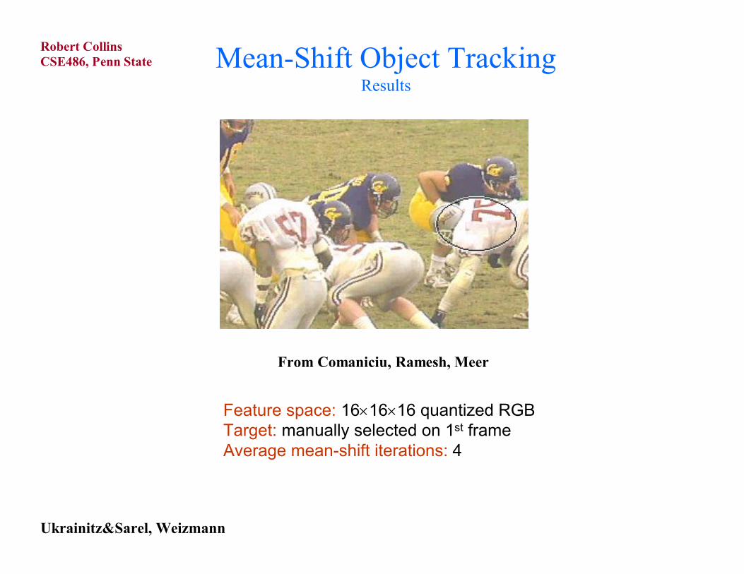
Mean-Shift Object TrackingResults
Feature space: 161616 quantized RGBTarget: manually selected on 1st frameAverage mean-shift iterations: 4
Ukrainitz&Sarel, Weizmann
From Comaniciu, Ramesh, Meer

CSE486, Penn StateRobert Collins
Mean-Shift Object TrackingResults
Partial occlusion Distraction Motion blur
Ukrainitz&Sarel, Weizmann

CSE486, Penn StateRobert Collins
Mean-Shift Object TrackingResults
Ukrainitz&Sarel, Weizmann
From Comaniciu, Ramesh, Meer

CSE486, Penn StateRobert Collins
Mean-Shift Object TrackingResults
Feature space: 128128 quantized RG
Ukrainitz&Sarel, Weizmann
From Comaniciu, Ramesh, Meer

CSE486, Penn StateRobert Collins
Mean-Shift Object TrackingResults
Feature space: 128128 quantized RG
Ukrainitz&Sarel, Weizmann
From Comaniciu, Ramesh, Meer
The man himself…


