Factor Models
Factor Models
MIT 18.S096
Dr. Kempthorne
Fall 2013
MIT 18.S096
Lecture 15:
Factor Models 1
Factor Models
Linear Factor ModelMacroeconomic Factor ModelsFundamental Factor ModelsStatistical Factor Models: Factor AnalysisPrincipal Components AnalysisStatistical Factor Models: Principal Factor Method
Outline
1 Factor ModelsLinear Factor ModelMacroeconomic Factor ModelsFundamental Factor ModelsStatistical Factor Models: Factor AnalysisPrincipal Components AnalysisStatistical Factor Models: Principal Factor Method
MIT 18.S096 Factor Models 2
Factor Models
Linear Factor ModelMacroeconomic Factor ModelsFundamental Factor ModelsStatistical Factor Models: Factor AnalysisPrincipal Components AnalysisStatistical Factor Models: Principal Factor Method
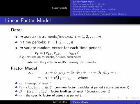
Linear Factor Model
Data:
m assets/instruments/indexes: i = 1, 2, . . . ,m
n time periods: t = 1, 2, . . . , n
m-variate random vector for each time period:xt = (x1,t , x2,t , . . . , xm,t)
′E.g., returns on m stocks/futures/currencies;
interest-rate yields on m US Treasury instruments.
Factor Modelxi ,t = αi + β1,i f1,t + β2,i f2,t + · · ·+ βk,i fk,t + εi ,t
= αi + β′i ft + εi ,t where
αi : intercept of asset i
ft = (f1,t , f2,t , . . . , fK ,t)′: common factor variables at period t (constant over i)
βi = (β1,i , . . . , βK ,i )′: factor loadings of asset i (constant over t)
εi,t : the specific factor of asset i at period t.
MIT 18.S096 Factor Models 3
Factor Models
Linear Factor ModelMacroeconomic Factor ModelsFundamental Factor ModelsStatistical Factor Models: Factor AnalysisPrincipal Components AnalysisStatistical Factor Models: Principal Factor Method
Linear Factor Model
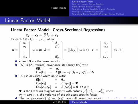
Linear Factor Model: Cross-Sectional Regressionsxt = α + Bft + εt ,
for each t ∈ 1, 2 . . . ,T, whereα1
α2
α = . (m 1); B =.
×
β′ ε , 1 1 t β2′
.αm
..
.
β′
m
=[[βi,k
]] ε2,t (m × K); εt =
. 1)..
ε
m,
(m ×
t
α and B are the same for all t.ft is (K−variate) covariance stationary I (0) with
E [ft ] = µfCov [ft ] = E [(ft − µf )(ft − µf )′] = Ωf
εt is m-variate white noise with:E [εt ] = 0m
Cov [εt ] = E [εtε′t ] = ΨCov [εt , εt′ ] = E [εtε′ ] = 0
t′ ∀t 6= t′
Ψ is the (m ×m) diagonal matrix with entries (σ2, σ2, . . . , σ2 ) where1 2 mσ2 = var(εi i,t), the variance of the ith asset specific factor.The two processes ft and εt have null cross-covariances:
E [(ft − µf )(εt′ − 0m)′] =MIT 18.S096 Factor Models 4
Factor Models
Linear Factor ModelMacroeconomic Factor ModelsFundamental Factor ModelsStatistical Factor Models: Factor AnalysisPrincipal Components AnalysisStatistical Factor Models: Principal Factor Method
Linear Factor Model
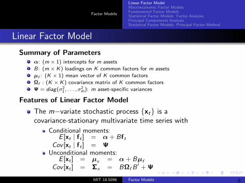
Summary of Parametersα: (m × 1) intercepts for m assets
B: (m × K) loadings on K common factors for m assets
µf : (K × 1) mean vector of K common factors
Ωf : (K × K) covariance matrix of K common factors
Ψ = diag(σ2, . . . , σ2m): m asset-specific variances1
Features of Linear Factor Model
The m−variate stochastic process xt is acovariance-stationary multivariate time series with
Conditional moments:E [xt | ft ] = α + Bft
Cov [xt | ft ] = ΨUnconditional moments:
E [xt ] = µx = α + Bµf
Cov [xt ] = Σx = BΩf B′ + Ψ
MIT 18.S096 Factor Models 5
Factor Models
Linear Factor ModelMacroeconomic Factor ModelsFundamental Factor ModelsStatistical Factor Models: Factor AnalysisPrincipal Components AnalysisStatistical Factor Models: Principal Factor Method
Linear Factor Model
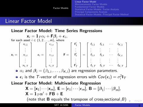
Linear Factor Model: Time Series Regressionsxi = 1Tαi + Fβi + εi ,
for each asseti ∈ 1, 2 .. . ,m,ε
wherex · · f
x =
i,1 f′ . ..
f f ·
i xi,t i =.
ε
i,t 1 1,
.. K ,1
.. 1 2,1
. . . .. . . . . . . . . . εi,t′
.
= ft. ..
T
F .. ..
x1, εi,T
f′
= f1,t f2,t · · · fK ,t . . . .. . . .. . . .
f1,T f2,T · · · fT K ,T
αi and βi = (β1,i , . . . , βK ,i ) are regression parameters.
εi is the T -vector of regression errors with Cov(εi ) = σ2i IT
Linear Factor Model: Multivariate RegressionX = [x1| · · · |xm], E = [ε1| · · · |εm], B = [β1| · · · |βm],X = 1Tα
′ + FB + E(note that B equals the transpose of cross-sectional B)
MIT 18.S096 Factor Models 6
Factor Models
Linear Factor ModelMacroeconomic Factor ModelsFundamental Factor ModelsStatistical Factor Models: Factor AnalysisPrincipal Components AnalysisStatistical Factor Models: Principal Factor Method
Outline
1 Factor ModelsLinear Factor ModelMacroeconomic Factor ModelsFundamental Factor ModelsStatistical Factor Models: Factor AnalysisPrincipal Components AnalysisStatistical Factor Models: Principal Factor Method
MIT 18.S096 Factor Models 7
Factor Models
Linear Factor ModelMacroeconomic Factor ModelsFundamental Factor ModelsStatistical Factor Models: Factor AnalysisPrincipal Components AnalysisStatistical Factor Models: Principal Factor Method
Macroeconomic Factor Models
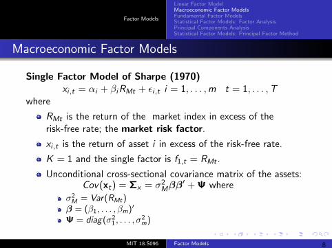
Single Factor Model of Sharpe (1970)xi ,t = αi + βiRMt + εi ,t i = 1, . . . ,m t = 1, . . . ,T
where
RMt is the return of the market index in excess of therisk-free rate; the market risk factor.
xi ,t is the return of asset i in excess of the risk-free rate.
K = 1 and the single factor is f1,t = RMt .
Unconditional cross-sectional covariance matrix of the assets:Cov(xt) = Σx = σ2
Mββ′ + Ψ where
σ2M = Var(RMt)
β = (β1, . . . , βm)′
Ψ = diag(σ21 , . . . , σ
2m)
MIT 18.S096 Factor Models 8
Factor Models
Linear Factor ModelMacroeconomic Factor ModelsFundamental Factor ModelsStatistical Factor Models: Factor AnalysisPrincipal Components AnalysisStatistical Factor Models: Principal Factor Method
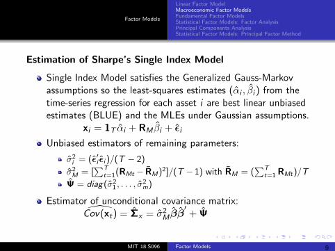
Estimation of Sharpe’s Single Index Model
Single Index Model satisfies the Generalized Gauss-Markovassumptions so the least-squares estimates (αi , βi ) from thetime-series regression for each asset i are best linear unbiasedestimates (BLUE) and the MLEs under Gaussian assumptions.
x ˆi = 1T αi + RMβi + εi
Unbiased estimators of remaining parameters:
σ2i = (ε′i εi )/(T − 2)
σ2M = [
∑Tt=1(RMt − RM)2]/(T − 1) with RM = (
∑Tt=1 RMt)/T
Ψ = diag(σ21 , . . . , σ
2m)
Estimator of unconditional covariance matrix:Cov(xt) = Σx = σ2 ˆ
Mββ′
+ Ψ
MIT 18.S096 Factor Models 9

Factor Models
Linear Factor ModelMacroeconomic Factor ModelsFundamental Factor ModelsStatistical Factor Models: Factor AnalysisPrincipal Components AnalysisStatistical Factor Models: Principal Factor Method
Macroeconomic Multifactor ModelThe common factor variables ft are realized values of macroecononomic variables, such as
Market riskPrice indices (CPI, PPI, commodities) / InflationIndustrial production (GDP)Money growthInterest ratesHousing startsUnemploymentSee Chen, Ross, Roll (1986). “Economic Forces and the Stock Market”
Linear Factor Model as Time Series Regressionsxi = 1Tαi + Fβi + εi , where
F = [f1, f2, . . . fT ]′ is the (T × K ) matrix of realized values of(K > 0) macroeconomic factors.Unconditional cross-sectional covariance matrix of the assets:
Cov(xt) = BΩf B′ + Ψ
where B = (β1, . . . ,βm)′ is (m × K )
MIT 18.S096 Factor Models 10
Factor Models
Linear Factor ModelMacroeconomic Factor ModelsFundamental Factor ModelsStatistical Factor Models: Factor AnalysisPrincipal Components AnalysisStatistical Factor Models: Principal Factor Method
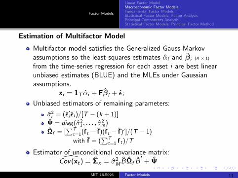
Estimation of Multifactor Model
Multifactor model satisfies the Generalized Gauss-Markovassumptions so the least-squares estimates αi and βi (K × 1)
from the time-series regression for each asset i are best linearunbiased estimates (BLUE) and the MLEs under Gaussianassumptions.
x βi = 1T αi + F i + εi
Unbiased estimators of remaining parameters:
σ2i = (ε′i εi )/[T − (k + 1)]
Ψ = diag(σ21 , . . . , σ
2m)
Ωf = [∑T
t=1(ft − f)(∑ft − f)′]/(T − 1)
with f T= ( t=1 ft)/T
Estimator of unconditional covariance matrix:Cov(xt) = Σ 2 ˆ ˆ ˆ ˆ
x = σ BΩf B′
M + Ψ
MIT 18.S096 Factor Models 11
Factor Models
Linear Factor ModelMacroeconomic Factor ModelsFundamental Factor ModelsStatistical Factor Models: Factor AnalysisPrincipal Components AnalysisStatistical Factor Models: Principal Factor Method
Outline
1 Factor ModelsLinear Factor ModelMacroeconomic Factor ModelsFundamental Factor ModelsStatistical Factor Models: Factor AnalysisPrincipal Components AnalysisStatistical Factor Models: Principal Factor Method
MIT 18.S096 Factor Models 12
Factor Models
Linear Factor ModelMacroeconomic Factor ModelsFundamental Factor ModelsStatistical Factor Models: Factor AnalysisPrincipal Components AnalysisStatistical Factor Models: Principal Factor Method
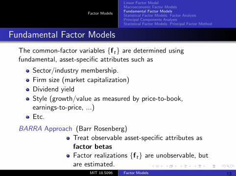
Fundamental Factor Models
The common-factor variables ft are determined usingfundamental, asset-specific attributes such as
Sector/industry membership.
Firm size (market capitalization)
Dividend yield
Style (growth/value as measured by price-to-book,earnings-to-price, ...)
Etc.
BARRA Approach (Barr Rosenberg)
Treat observable asset-specific attributes asfactor betasFactor realizations ft are unobservable, butare estimated.
MIT 18.S096 Factor Models 13
Factor Models
Linear Factor ModelMacroeconomic Factor ModelsFundamental Factor ModelsStatistical Factor Models: Factor AnalysisPrincipal Components AnalysisStatistical Factor Models: Principal Factor Method
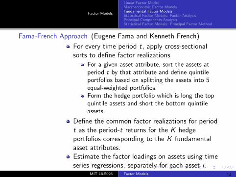
Fama-French Approach (Eugene Fama and Kenneth French)
For every time period t, apply cross-sectionalsorts to define factor realizations
For a given asset attribute, sort the assets atperiod t by that attribute and define quintileportfolios based on splitting the assets into 5equal-weighted portfolios.Form the hedge portfolio which is long the topquintile assets and short the bottom quintileassets.
Define the common factor realizations for periodt as the period-t returns for the K hedgeportfolios corresponding to the K fundamentalasset attributes.Estimate the factor loadings on assets using timeseries regressions, separately for each asset i .
MIT 18.S096 Factor Models 14
Factor Models
Linear Factor ModelMacroeconomic Factor ModelsFundamental Factor ModelsStatistical Factor Models: Factor AnalysisPrincipal Components AnalysisStatistical Factor Models: Principal Factor Method
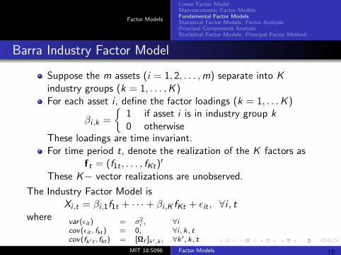
Barra Industry Factor Model
Suppose the m assets (i = 1, 2, . . . ,m) separate into Kindustry groups (k = 1, . . . ,K )For each asset i, define the factor loadings (k = 1, . . .K )
1 if asset i is in industry group kβi ,k =
0 otherwiseThese loadings are time invariant.For time period t, denote the realization of the K factors as
ft = (f1t , . . . , fKt)′
These K− vector realizations are unobserved.
The Industry Factor Model isXi ,t = βi ,1f1t + · · ·+ βi ,K fKt + εit , ∀i , t
wherevar(ε 2
it) = σ ,i ∀icov(εit , fkt) = 0, ∀i , k, tcov(fk′t , fkt) = [Ωf ]k′,k , ∀k ′, k, t
MIT 18.S096 Factor Models 15
Factor Models
Linear Factor ModelMacroeconomic Factor ModelsFundamental Factor ModelsStatistical Factor Models: Factor AnalysisPrincipal Components AnalysisStatistical Factor Models: Principal Factor Method
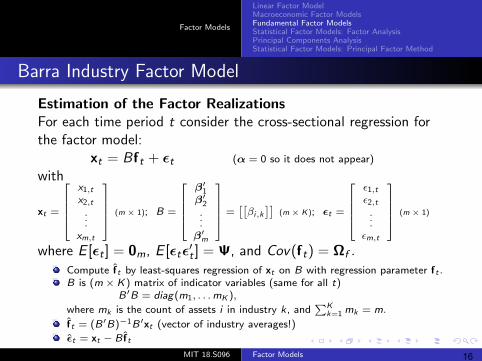
Barra Industry Factor Model
Estimation of the Factor RealizationsFor each time period t consider the cross-sectional regression forthe factor model:
xt = Bft + εt (α = 0 so it does not appear)
with
xt =
x1,t
β1′ ε1,t x2,t β′2 [[ ]] ε2,t . (m × 1); B = . = βi,k (m ε 1)
.× K); t =
.
.
(m
.×
. .
m
.
x ,t β′
m εm,t
where E [εt ] = 0m, E [εtε
′t ] = Ψ, and Cov(ft) = Ωf
.
Compute ft by least-squares regression of xt on B with regression parameter ft .B is (m × K) matrix of indicator variables (same for all t)
B′B = diag(m1, . . .mK ),
where mk is the count of assets i in industry k, and∑K
k=1 mk = m.
ft = (B′B)−1B′xt (vector of industry averages!)
εt = xt − B ft
MIT 18.S096 Factor Models 16
Factor Models
Linear Factor ModelMacroeconomic Factor ModelsFundamental Factor ModelsStatistical Factor Models: Factor AnalysisPrincipal Components AnalysisStatistical Factor Models: Principal Factor Method
Barra Industry Factor Model
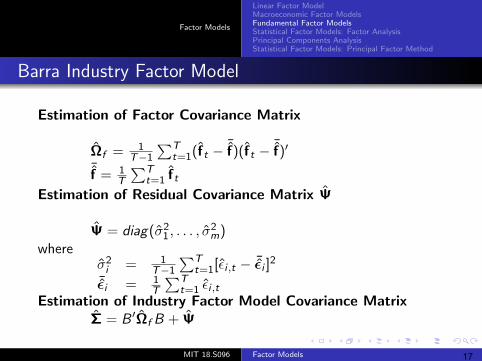
Estimation of Factor Covariance Matrix
Ωf = 1T−1
∑Tt=1(ft − ¯f)(ft − ¯f)′
¯f = 1 fT
∑T ˆt=1 t
Estimation of Residual Covariance Matrix Ψ
Ψ = diag(σ21, . . . , σ
2m)
whereσ2i = 1
T−1
∑Tt=1[εi ,t − ¯εi ]
2
¯εi = 1 TT
∑t=1 εi ,t
Estimation of Industry Factor Model Covariance MatrixΣ = B ′Ωf B + Ψ
MIT 18.S096 Factor Models 17
Factor Models
Linear Factor ModelMacroeconomic Factor ModelsFundamental Factor ModelsStatistical Factor Models: Factor AnalysisPrincipal Components AnalysisStatistical Factor Models: Principal Factor Method
Barra Industry Factor Model
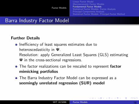
Further Details
Inefficiency of least squares estimates due toheteroscedasticity in Ψ.Resolution: apply Generalized Least Squares (GLS) estimatingΨ in the cross-sectional regressions.
The factor realizations can be rescaled to represent factormimicking portfolios
The Barra Industry Factor Model can be expressed as aseemingly unrelated regression (SUR) model
MIT 18.S096 Factor Models 18
Factor Models
Linear Factor ModelMacroeconomic Factor ModelsFundamental Factor ModelsStatistical Factor Models: Factor AnalysisPrincipal Components AnalysisStatistical Factor Models: Principal Factor Method
Outline
1 Factor ModelsLinear Factor ModelMacroeconomic Factor ModelsFundamental Factor ModelsStatistical Factor Models: Factor AnalysisPrincipal Components AnalysisStatistical Factor Models: Principal Factor Method
MIT 18.S096 Factor Models 19
Factor Models
Linear Factor ModelMacroeconomic Factor ModelsFundamental Factor ModelsStatistical Factor Models: Factor AnalysisPrincipal Components AnalysisStatistical Factor Models: Principal Factor Method
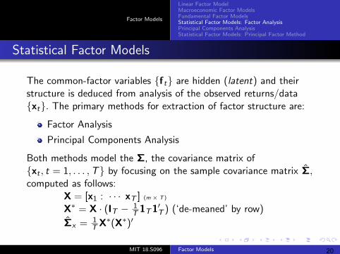
Statistical Factor Models
The common-factor variables ft are hidden (latent) and theirstructure is deduced from analysis of the observed returns/dataxt. The primary methods for extraction of factor structure are:
Factor Analysis
Principal Components Analysis
Both methods model the Σ, the covariance matrix ofxt , t = 1, . . . ,T by focusing on the sample covariance matrix Σ,computed as follows:
X = [x1 : · · · xT ] (m × T )
X∗ = X · (IT − 1T 1T1′T ) (‘de-meaned’ by row)
Σx = 1 XT∗(X∗)′
MIT 18.S096 Factor Models 20
Factor Models
Linear Factor ModelMacroeconomic Factor ModelsFundamental Factor ModelsStatistical Factor Models: Factor AnalysisPrincipal Components AnalysisStatistical Factor Models: Principal Factor Method
Factor Analysis Model
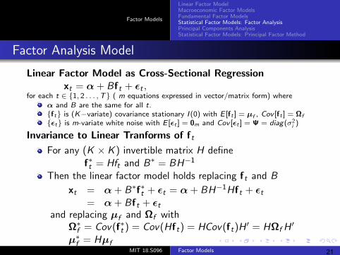
Linear Factor Model as Cross-Sectional Regressionxt = α + Bft + εt ,
for each t ∈ 1, 2 . . . ,T ( m equations expressed in vector/matrix form) whereα and B are the same for all t.ft is (K−variate) covariance stationary I (0) with E [ft ] = µf , Cov [ft ] = Ωf
εt is m-variate white noise with E [εt ] = 0m and Cov [ε 2t ] = Ψ = diag(σ )i
Invariance to Linear Tranforms of ft
For any (K × K ) invertible matrix H definef∗t = Hft and B∗ = BH−1
Then the linear factor model holds replacing ft and B
xt = α + B∗f∗t + εt = α + BH−1Hft + εt= α + Bft + εt
and replacing µf and Ωf withΩ∗f = Cov(f∗t ) = Cov(Hft) = HCov(ft)H ′ = HΩfH
′
µ∗f = HµfMIT 18.S096 Factor Models 21
Factor Models
Linear Factor ModelMacroeconomic Factor ModelsFundamental Factor ModelsStatistical Factor Models: Factor AnalysisPrincipal Components AnalysisStatistical Factor Models: Principal Factor Method
Factor Analysis Model
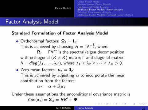
Standard Formulation of Factor Analysis Model
Orthonormal factors: Ωf = IKThis is achieved by choosing H = ΓΛ−
12 , where
Ωf = ΓΛΓ′ is the spectral/eigen decompositionwith orthogonal (K × K ) matrix Γ and diagonal matrixΛ = diag(λ1, . . . , λK ), where λ1 ≥ λ2 ≥ · · · ≥ λK > 0.
Zero-mean factors: µf = 0K
This is achieved by adjusting α to incorporate the meancontribution from the factors:
α∗ = α + Bµf
Under these assumptions the unconditional covariance matrix isCov(xt) = Σx = BB ′ + Ψ
MIT 18.S096 Factor Models 22
Factor Models
Linear Factor ModelMacroeconomic Factor ModelsFundamental Factor ModelsStatistical Factor Models: Factor AnalysisPrincipal Components AnalysisStatistical Factor Models: Principal Factor Method
Factor Analysis Model
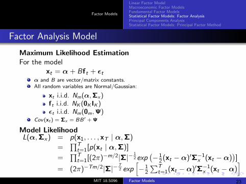
Maximum Likelihood EstimationFor the model
xt = α + Bft + εtα and B are vector/matrix constants.All random variables are Normal/Gaussian:
xt i.i.d. Nm(α,Σx)ft i.i.d. NK (0K IK )εt i.i.d. Nm(0m,Ψ)
Cov(xt) = Σx = BB′ + Ψ
Model LikelihoodL(α,Σx) = p∏(x1, . . . , xT | α,Σ)
T= ∏t=1[p(xt | α,Σ)]T 1
= t=1[(2π)−m/2|Σ|− 2 exp(−1 (xt α) Σ 1(xt α) ]2
TTm
− ′ −x −
= (2π)− /2|Σ|−
)2 exp
[−1
2
∑Tt=1(xt −α)′Σ−1
x (xt −α)]
MIT 18.S096 Factor Models 23
Factor Models
Linear Factor ModelMacroeconomic Factor ModelsFundamental Factor ModelsStatistical Factor Models: Factor AnalysisPrincipal Components AnalysisStatistical Factor Models: Principal Factor Method
Factor Analysis Model
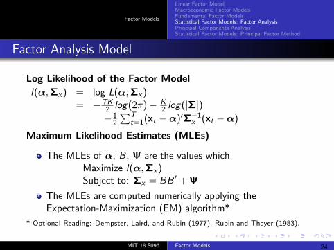
Log Likelihood of the Factor Model
l(α,Σx) = log L(α,Σx)
= −TK2 log(2π)− K
2 log(|Σ|)−1 T
2
∑t=1(xt −α)′Σ−1
x (xt −α)
Maximum Likelihood Estimates (MLEs)
The MLEs of α, B, Ψ are the values whichMaximize l(α,Σx)Subject to: Σx = BB ′ + Ψ
The MLEs are computed numerically applying theExpectation-Maximization (EM) algorithm*
* Optional Reading: Dempster, Laird, and Rubin (1977), Rubin and Thayer (1983).
MIT 18.S096 Factor Models 24
Factor Models
Linear Factor ModelMacroeconomic Factor ModelsFundamental Factor ModelsStatistical Factor Models: Factor AnalysisPrincipal Components AnalysisStatistical Factor Models: Principal Factor Method
Factor Analysis Model
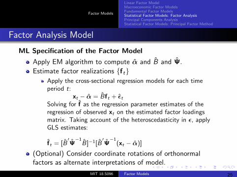
ML Specification of the Factor Model
Apply EM algorithm to compute α and B and Ψ.
Estimate factor realizations ftApply the cross-sectional regression models for each timeperiod t:
xt − α = Bft + εtSolving for f as the regression parameter estimates of theregression of observed xt on the estimated factor loadingsmatrix. Taking account of the heteroscedasticity in ε, applyGLS estimates:
f = [B′ 1Ψ− ˆ
t B]−1[B′Ψ−1
(xt − α)]
(Optional) Consider coordinate rotations of orthonormalfactors as alternate interpretations of model.
MIT 18.S096 Factor Models 25
Factor Models
Linear Factor ModelMacroeconomic Factor ModelsFundamental Factor ModelsStatistical Factor Models: Factor AnalysisPrincipal Components AnalysisStatistical Factor Models: Principal Factor Method
Factor Analysis Model
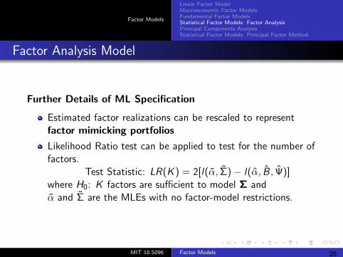
Further Details of ML Specification
Estimated factor realizations can be rescaled to representfactor mimicking portfolios
Likelihood Ratio test can be applied to test for the number offactors.
Test Statistic: LR(K ) = 2[l(α,Σ)˜ − l(α, B,Ψ)]ˆ
where H0: K factors are sufficient to model Σ andα and Σ are the MLEs with no factor-model restrictions.
MIT 18.S096 Factor Models 26
Factor Models
Linear Factor ModelMacroeconomic Factor ModelsFundamental Factor ModelsStatistical Factor Models: Factor AnalysisPrincipal Components AnalysisStatistical Factor Models: Principal Factor Method
Outline
1 Factor ModelsLinear Factor ModelMacroeconomic Factor ModelsFundamental Factor ModelsStatistical Factor Models: Factor AnalysisPrincipal Components AnalysisStatistical Factor Models: Principal Factor Method
MIT 18.S096 Factor Models 27
Factor Models
Linear Factor ModelMacroeconomic Factor ModelsFundamental Factor ModelsStatistical Factor Models: Factor AnalysisPrincipal Components AnalysisStatistical Factor Models: Principal Factor Method
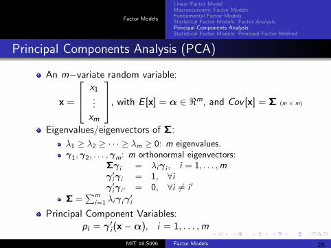
Principal Components Analysis (PCA)
An m−va riate random variable:
x = x1 ...
, with E [x] = α ∈ <m, and Cov [x] = Σ (m × m)
xmEigenvalues/eigenvectors of Σ:
λ1 ≥ λ2 ≥ · · · ≥ λm ≥ 0: m eigenvalues.γ1,γ2, . . . ,γm: m orthonormal eigenvectors:
Σγ i = λiγ i , i = 1, . . . ,mγ′iγ i = 1, ∀iγ′iγ i = 0,′ ∀i 6= i ′
Σ =∑m
i=1 λiγ iγ′i
Principal Component Variables:pi = γ ′i (x−α), i = 1, . . . ,m
MIT 18.S096 Factor Models 28
Factor Models
Linear Factor ModelMacroeconomic Factor ModelsFundamental Factor ModelsStatistical Factor Models: Factor AnalysisPrincipal Components AnalysisStatistical Factor Models: Principal Factor Method
Principal Components Analysis
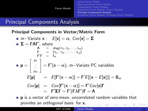
Principal Components in Vector/Matrix Form
m−Variate x : E [x] = α, Cov [x] = ΣΣ = ΓΛΓ′, where
Λ = diag(λ1, λ2, . . . , λm)Γ = [γ1 : γ2 : · · · : γm]Γ′Γ = Im
p
p1
= .. ), m.
= Γ′(x−α −Variate PC variablespm
E [p] = E [Γ′(x−α)] = Γ′E [(x− E [x])] = 0m
Cov [p] = Cov [Γ′(x−α)] = Γ′Cov [x]Γ= Γ′ΣΓ = Γ′(ΓλΓ′)Γ = Λ
p is a vector of zero-mean, uncorrelated random variables thatprovides an orthogonal basis for x.
MIT 18.S096 Factor Models 29
Factor Models
Linear Factor ModelMacroeconomic Factor ModelsFundamental Factor ModelsStatistical Factor Models: Factor AnalysisPrincipal Components AnalysisStatistical Factor Models: Principal Factor Method
Principal Components Analysis
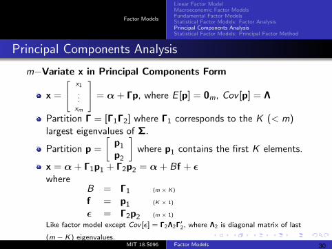
m−Variate x in Principal Components Formx
x =
1 ..
= α + Γp, where E [p] = 0m, Cov [p] = Λ.
xm
Partition Γ = [Γ1Γ2] where Γ1 corresponds to the K (< m)largest eigenvalues of Σ.
pPartition p =
[1
p2
]where p1 contains the first K elements.
x = α + Γ1p1 + Γ2p2 = α + Bf + εwhere
B = Γ1 (m × K)
f = p1 (K × 1)
ε = Γ2p2 (m × 1)
Like factor model except Cov [ε] = Γ2Λ2Γ′2, where Λ2 is diagonal matrix of last
(m − K) eigenvalues.MIT 18.S096 Factor Models 30
Factor Models
Linear Factor ModelMacroeconomic Factor ModelsFundamental Factor ModelsStatistical Factor Models: Factor AnalysisPrincipal Components AnalysisStatistical Factor Models: Principal Factor Method
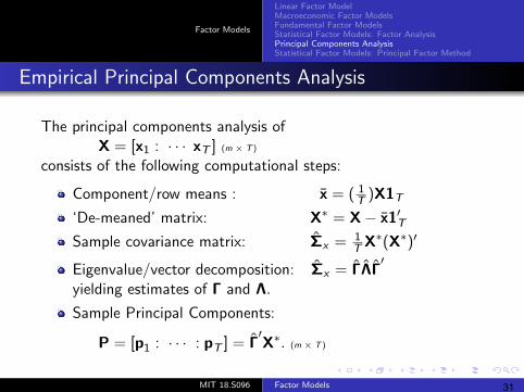
Empirical Principal Components Analysis
The principal components analysis ofX = [x1 : · · · xT ] (m × T )
consists of the following computational steps:
Component/row means : x = ( 1 )X1T T
‘De-meaned’ matrix: X∗ = X− x1′TSample covariance matrix: Σx = 1 XT
∗(X∗)′
Eigenvalue/vector decomposition: Σx = ΓΛΓ′
yielding estimates of Γ and Λ.
Sample Principal Components:
P = [p1 : · · · : pT ] = Γ′X∗. (m × T )
MIT 18.S096 Factor Models 31
Factor Models
Linear Factor ModelMacroeconomic Factor ModelsFundamental Factor ModelsStatistical Factor Models: Factor AnalysisPrincipal Components AnalysisStatistical Factor Models: Principal Factor Method
Empirical Principal Components Analysis
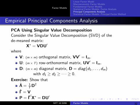
PCA Using Singular Value DecompositionConsider the Singular Value Decomposition (SVD) of thede-meaned matrix:
X∗ = VDU′
where
V: (m ×m) orthogonal matrix, VV′ = Im.
U: (m × T ) row-orthonormal matrix, UV′ = Im.
D: (m ×m) diagonal matrix, D = diag(d1, . . . , dm)with d1 ≥ d2 ≥ · · · ≥ 0.
Exercise: Show that
Λ = 1T D2
Γ = V
P = Γ′X∗ = DU′
MIT 18.S096 Factor Models 32
Factor Models
Linear Factor ModelMacroeconomic Factor ModelsFundamental Factor ModelsStatistical Factor Models: Factor AnalysisPrincipal Components AnalysisStatistical Factor Models: Principal Factor Method
Alternate Definition of PC Variables
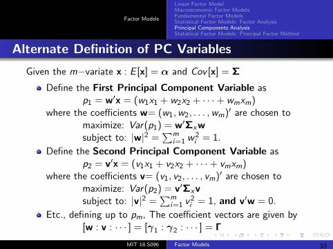
Given the m−variate x : E [x] = α and Cov [x] = Σ
Define the First Principal Component Variable asp1 = w′x = (w1x1 + w2x2 + · · ·+ wmxm)
where the coefficients w= (w1,w2, . . . ,wm)′ are chosen tomaximize: Var(p1)∑= w′Σxwsubject to: |w|2 m= i=1 w
2i = 1.
Define the Second Principal Component Variable asp2 = v′x = (v1x1 + v2x2 + · · ·+ vmxm)
where the coefficients v= (v1, v2, . . . , vm)′ are chosen tomaximize: Var(p2)∑= v′Σxv
msubject to: |v|2 = i=1 v2i = 1, and v′w = 0.
Etc., defining up to pm, The coefficient vectors are given by[w : v : · · · ] = [γ1 : γ2 : · · · ] = Γ
MIT 18.S096 Factor Models 33
Factor Models
Linear Factor ModelMacroeconomic Factor ModelsFundamental Factor ModelsStatistical Factor Models: Factor AnalysisPrincipal Components AnalysisStatistical Factor Models: Principal Factor Method
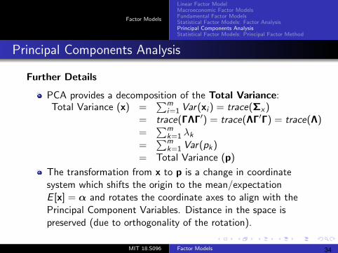
Principal Components Analysis
Further Details
PCA provides a decomposition of the Total Variance:Total Variance (x m) =
=
∑i=1 Var(xi ) = trace(Σx)
trace∑ (ΓΛΓ′) = trace(ΛΓ′Γ) = trace(Λ)m= k=1 λkm=
=
∑k=1 Var(pk)
Total Variance (p)
The transformation from x to p is a change in coordinatesystem which shifts the origin to the mean/expectationE [x] = α and rotates the coordinate axes to align with thePrincipal Component Variables. Distance in the space ispreserved (due to orthogonality of the rotation).
MIT 18.S096 Factor Models 34
Factor Models
Linear Factor ModelMacroeconomic Factor ModelsFundamental Factor ModelsStatistical Factor Models: Factor AnalysisPrincipal Components AnalysisStatistical Factor Models: Principal Factor Method
Outline
1 Factor ModelsLinear Factor ModelMacroeconomic Factor ModelsFundamental Factor ModelsStatistical Factor Models: Factor AnalysisPrincipal Components AnalysisStatistical Factor Models: Principal Factor Method
MIT 18.S096 Factor Models 35
Factor Models
Linear Factor ModelMacroeconomic Factor ModelsFundamental Factor ModelsStatistical Factor Models: Factor AnalysisPrincipal Components AnalysisStatistical Factor Models: Principal Factor Method
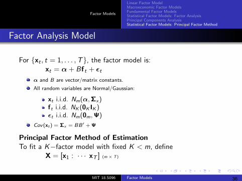
Factor Analysis Model
For xt , t = 1, . . . ,T, the factor model is:xt = α + Bft + εt
α and B are vector/matrix constants.
All random variables are Normal/Gaussian:
xt i.i.d. Nm(α,Σx)ft i.i.d. NK (0K IK )εt i.i.d. Nm(0m,Ψ)
Cov(xt) = Σx = BB′ + Ψ
Principal Factor Method of EstimationTo fit a K−factor model with fixed K < m, define
X = [x1 : · · · xT ] (m × T )
MIT 18.S096 Factor Models 36

Factor Models
Linear Factor ModelMacroeconomic Factor ModelsFundamental Factor ModelsStatistical Factor Models: Factor AnalysisPrincipal Components AnalysisStatistical Factor Models: Principal Factor Method
Principal Factor Method of Estimation
Step 1: Conduct the computational steps of principalcomponents analysis:
Component/row means :x = ( 1T
)X1T
‘De-meaned’ matrix: X∗ = X− x1′TSample covariance matrix: Σx = 1
TX∗(X∗)′
Eigenvalue/vector decomposition: Σx = ΓΛΓ′
yielding estimates of Γ and Λ.
Step 2: Specify initial estimates (index s = 0)
α0 = xB0 = Γ(K)(Λ(K))
12 , where
Γ(K) is submatrix of Γ (first K columns)Λ(K) is submatrix of Λ (first K columns)
Ψ0 = diag(Σx)− diag(B ˜0B′0)
Σ0 = B ˜0B′0 + Ψ0
MIT 18.S096 Factor Models 37
Factor Models
Linear Factor ModelMacroeconomic Factor ModelsFundamental Factor ModelsStatistical Factor Models: Factor AnalysisPrincipal Components AnalysisStatistical Factor Models: Principal Factor Method
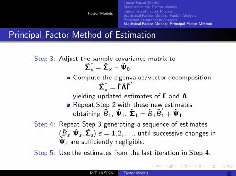
Principal Factor Method of Estimation
Step 3: Adjust the sample covariance matrix toΣ∗x = Σx − Ψ0
Compute the eigenvalue/vector decomposition:
Σ∗x = ΓΛΓ
′
yielding updated estimates of Γ and ΛRepeat Step 2 with these new estimatesobtaining B1, Ψ1, Σ1 = B ˜
1B′1 + Ψ1
Step 4: Repeat Step 3 generating a sequence of estimates(Bs , Ψs , Σs) s = 1, 2, . . ., until successive changes inΨs are sufficiently negligible.
Step 5: Use the estimates from the last iteration in Step 4.
MIT 18.S096 Factor Models 38

MIT OpenCourseWarehttp://ocw.mit.edu
18.S096 Topics in Mathematics with Applications in FinanceFall 2013
For information about citing these materials or our Terms of Use, visit: http://ocw.mit.edu/terms.


