
5/03/2018
1
Lecture 4Survey Research & Design in Psychology
James Neill, 2018Creative Commons Attribution 4.0
Image source: http://commons.wikimedia.org/wiki/File:Gnome-power-statistics.svg, GPL
Correlation
2
Howitt & Cramer (2014)● Ch 7: Relationships between two or more
variables: Diagrams and tables
● Ch 8: Correlation coefficients: Pearson
correlation and Spearman’s rho
● Ch 11: Statistical significance for the
correlation coefficient: A practical introduction
to statistical inference
● Ch 15: Chi-square: Differences between
samples of frequency data
● Note: Howitt and Cramer doesn't cover point bi-serial correlation
Readings
3
1Covariation
2Purpose of correlation
3Linear correlation
4Types of correlation
5Interpreting correlation
6Assumptions / limitations
Overview

5/03/2018
2
4
Covariation
e.g., pollen and bees
e.g., study and grades
e.g., nutrients and growth
The world is made of co-variations
We observe
covariations in
the psycho-
social world.
e.g., depictions of
violence in the
environment.
e.g., psychological
states such as
stress and
depression.
Measure
observations and
analyse their co-
occurrence
5/03/2018
3
Covariations are the basis
of more complex models
8
Purpose of correlation
9
The underlying purpose of
correlation is to help address the
question:
What is the
• relationship or
• association or
• shared variance or
• co-relationbetween two variables?
Purpose of correlation

5/03/2018
4
10
Other ways of expressing the
underlying correlational question
include:
To what extent do variables
• covary?
• depend on one another?
• explain one another?
Purpose of correlation
11
Linear correlation
12
r = -.76
Extent to which two variables have a
simple linear (straight-line) relationship.
Image source: http://commons.wikimedia.org/wiki/File:Scatterplot_r%3D-.76.png, Public domain
Linear correlation
5/03/2018
5
13
The linear relation between two variables is indicated by a correlation’s:
• Direction: Sign (+ / -) indicates direction
of relationship (+ve or -ve slope)
• Strength: Size indicates strength (values closer to -1 or +1 indicate greater strength)
• Statistical significance: p indicates
likelihood that the observed relationship
could have occurred by chance
Linear correlation
14
• No relationship (r ~ 0)
(X and Y are independent )
• Linear relationship
(X and Y are dependent)– As X ↑s, so does Y (r > 0)
– As X ↑s, Y ↓s (r < 0)
• Non-linear relationship
Types of correlation
15
There are many different
measures of correlation.
To decide which type of
correlation to use, consider
the levels of measurement
for each variable.
Types of correlation

5/03/2018
6
16
• Nominal by nominal:
Phi (Φ) / Cramer’s V, Chi-square
• Ordinal by ordinal:
Spearman’s rank / Kendall’s Tau b
• Dichotomous by interval/ratio:
Point bi-serial rpb
• Interval/ratio by interval/ratio:
Product-moment or Pearson’s r
Types of correlation
17
Scatterplot
Product-
moment correlation (r)
Interval/Ratio
⇐⇑Recode
Clustered bar
chart or scatterplot
Spearman's
Rho or Kendall's Tau
Ordinal
Clustered bar
chart or
scatterplotPoint bi-serial
correlation (rpb)
⇐ Recode
Clustered bar-chartChi-square,
Phi (φ) or Cramer's V
Nominal
Int/RatioOrdinalNominal
Types of correlation and LOM
18
Nominal by nominal
5/03/2018
7
19
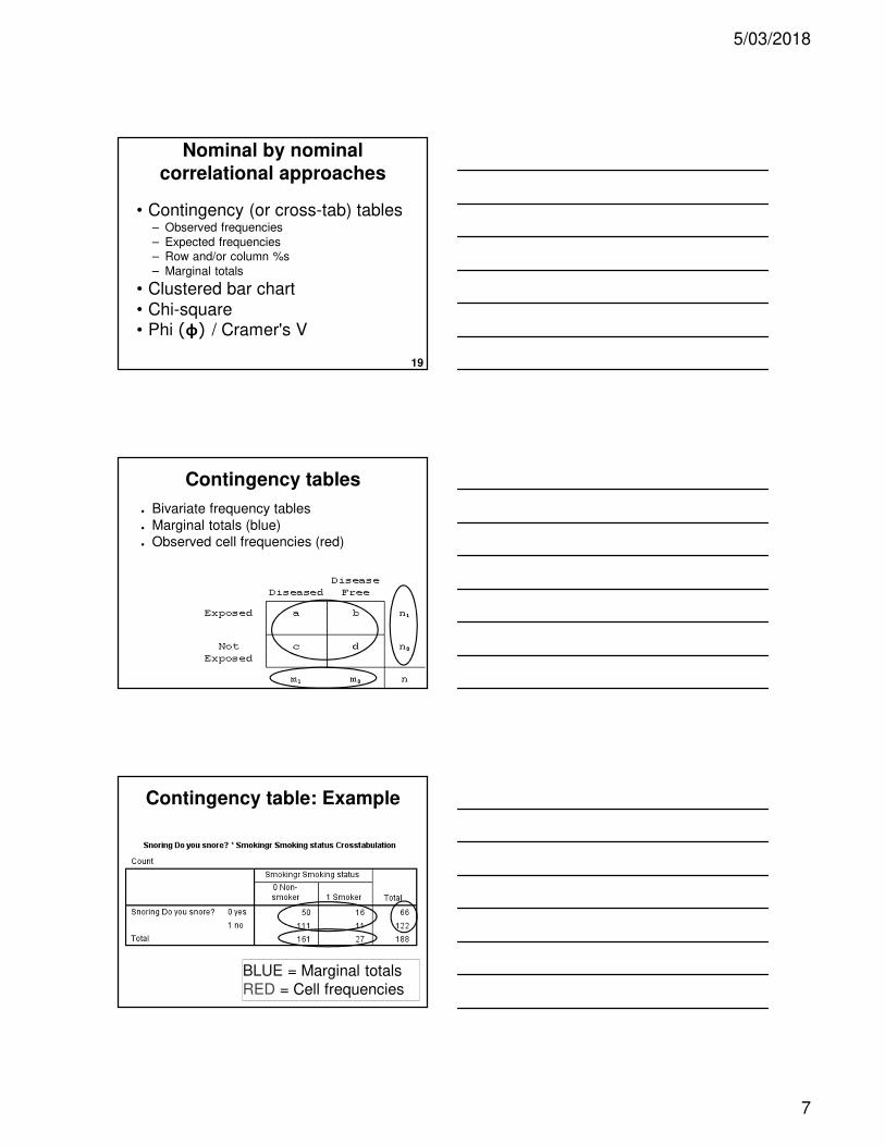
• Contingency (or cross-tab) tables– Observed frequencies
– Expected frequencies
– Row and/or column %s
– Marginal totals
• Clustered bar chart
• Chi-square• Phi (φ) / Cramer's V
Nominal by nominal
correlational approaches
● Bivariate frequency tables
● Marginal totals (blue)
● Observed cell frequencies (red)
Contingency tables
BLUE = Marginal totals
RED = Cell frequencies
Contingency table: Example

5/03/2018
8
●Expected counts are the cell frequencies that should
occur if the variables are not correlated.
●Chi-square is based on the squared differences
between the actual and expected cell counts.
2 2
22
- -
--
2
sum of ((observed – expected)2 / expected)χ 2=
Contingency table: Example
Row and/or column cell percentages can also be usefule.g., ~60% of smokers snore, whereas only ~30%d of non-smokers snore.
Cell percentages
Bivariate bar graph of frequencies or percentages.
The category
axis bars are
clustered (by
colour or fill
pattern) to
indicate the
second variable’s
categories.
Clustered bar graph

5/03/2018
9
~60% of
snorers are
smokers,
whereas only
~30% of non-
snores are
smokers.
Pearson chi-square test
Write-up: χ2 (1, 188) = 8.07, p = .004
Smoking (2) x Snoring (2)
Pearson chi-square test:
Example
5/03/2018
10
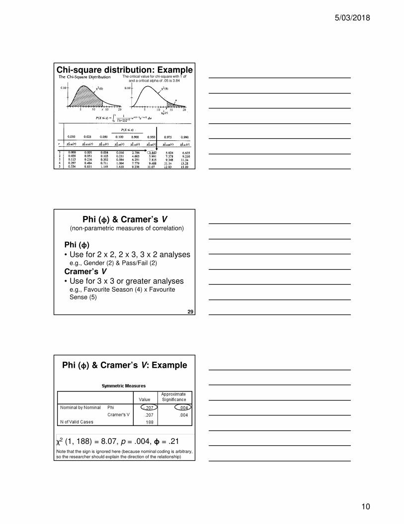
The critical value for chi-square with 1 dfand a critical alpha of .05 is 3.84
Chi-square distribution: Example
29
Phi (φ)
• Use for 2 x 2, 2 x 3, 3 x 2 analysese.g., Gender (2) & Pass/Fail (2)
Cramer’s V• Use for 3 x 3 or greater analyses
e.g., Favourite Season (4) x Favourite
Sense (5)
(non-parametric measures of correlation)
Phi (φ) & Cramer’s V
χ2 (1, 188) = 8.07, p = .004, φ = .21Note that the sign is ignored here (because nominal coding is arbitrary,
so the researcher should explain the direction of the relationship)
Phi (φ) & Cramer’s V: Example

5/03/2018
11
31
Ordinal by ordinal
32
• Spearman's rho (rs)• Kendall tau (τ)
• Alternatively, use nominal by
nominal techniques (i.e., recode the variables or treat them as
having a lower level of measurement)
Ordinal by ordinal
correlational approaches
33
• Ordinal by ordinal data is difficult to
visualise because it is non-
parametric, with many points.
• Consider using:–Non-parametric approaches
(e.g., clustered bar chart)
–Parametric approaches
(e.g., scatterplot with line of best fit)
Graphing ordinal by ordinal data
5/03/2018
12
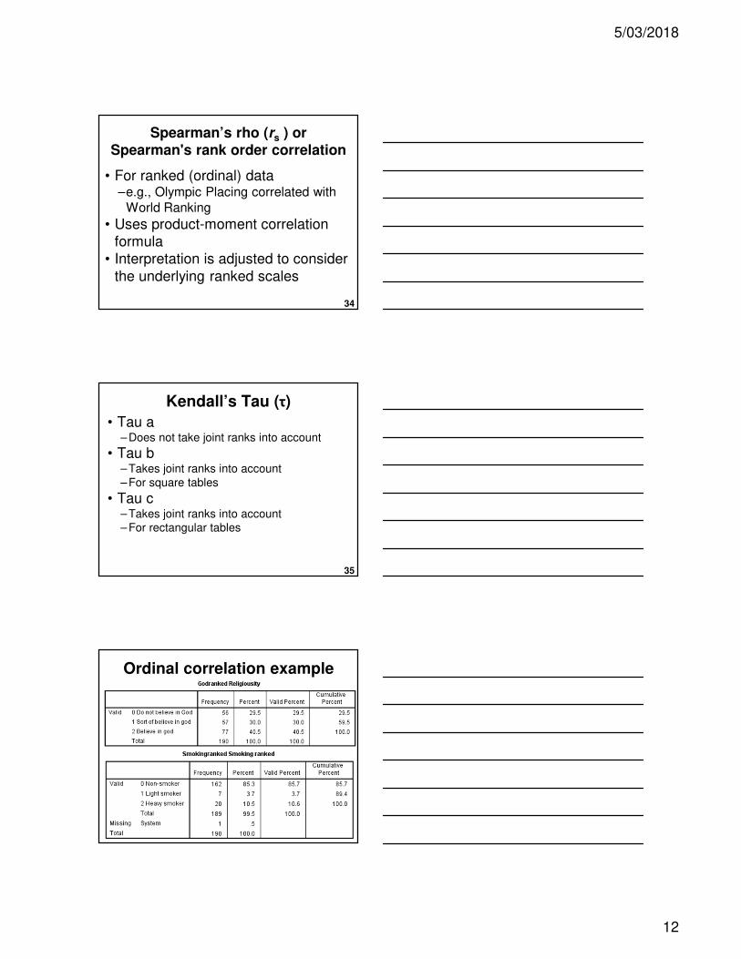
34
• For ranked (ordinal) data–e.g., Olympic Placing correlated with
World Ranking
• Uses product-moment correlation
formula
• Interpretation is adjusted to consider
the underlying ranked scales
Spearman’s rho (rs ) orSpearman's rank order correlation
35
• Tau a– Does not take joint ranks into account
• Tau b– Takes joint ranks into account
– For square tables
• Tau c– Takes joint ranks into account
– For rectangular tables
Kendall’s Tau (τ)
Ordinal correlation example

5/03/2018
13
Ordinal correlation example
τb = -.07, p = .298There is a small effect towards non-smokers being more likely to believe in God, but this could have occurred
through sampling error.
Ordinal correlation example
39
Dichotomous by interval/ratio
5/03/2018
14
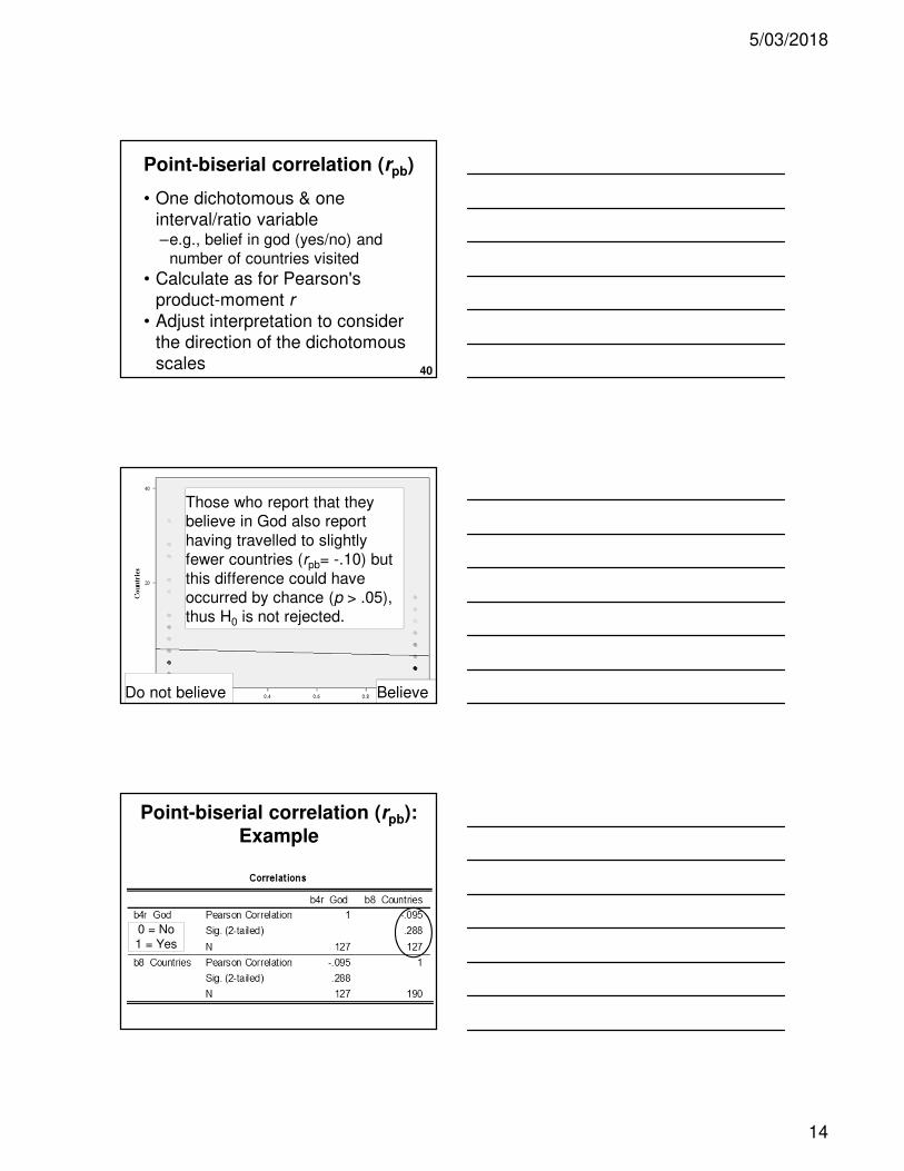
40
• One dichotomous & one
interval/ratio variable–e.g., belief in god (yes/no) and
number of countries visited
• Calculate as for Pearson's
product-moment r
• Adjust interpretation to consider
the direction of the dichotomous
scales
Point-biserial correlation (rpb)
Point-biserial correlation (rpb) :
ExampleThose who report that they
believe in God also report
having travelled to slightly
fewer countries (rpb= -.10) but
this difference could have
occurred by chance (p > .05),
thus H0 is not rejected.
Do not believe Believe
0 = No
1 = Yes
Point-biserial correlation (rpb):
Example

5/03/2018
15
43
Interval/ratio by interval/ratio
44
• Plot each pair of observations (X, Y) – x = predictor variable (independent; IV)
– y = criterion variable (dependent; DV)
• By convention:– IV on the x (horizontal) axis
– DV on the y (vertical) axis
• Direction of relationship:– +ve = trend from bottom left to top right
– -ve = trend from top left to bottom right
Scatterplot
Upward slope = positive correlation
Scatterplot showing relationship between
age & cholesterol with line of best fit

5/03/2018
16
46
• The correlation between 2
variables is a measure of the
degree to which pairs of numbers
(points) cluster together around a
best-fitting straight line
• Line of best fit: y = a + bx
• Check for:
– outliers
– linearity
Line of best fit
X-axis should be
IV (predictor)
Y-axis should be
DV (outcome)
What’s wrong with this scatterplot?
Strong positive (.81) Q: Why is infant mortality positively linearly associated
with the number of physicians (with the
effects of GDP
removed)?
A: Because more
doctors tend to be deployed to areas
with infant mortality (socio-economic
status aside).
Scatterplot example:

5/03/2018
17
Weak positive (.14)
Outlier –
exaggerating the correlation
Scatterplot example:
Moderately strong negative (-.76)
A: Having sufficient
Vitamin D (via sunlight)
lowers risk of cancer.
However, UV light exposure increases risk
of skin cancer.
Q: Why is there a
strong negative correlation
between solar radiation and
breast cancer?
Scatterplot example:
● The product-moment
correlation is the
standardised covariance.
Pearson product-moment
correlation (r)

5/03/2018
18
52
• Variance shared by 2 variables
• Covariance reflects the
direction of the relationship:+ve cov indicates +ve relationship
-ve cov indicates -ve relationship
● Covariance is unstandardised.
Cross products
N - 1 for the sample;
Covariance
-ve cro
ss
pro
duc
ts
-ve cross
products
-ve cross
products
+ve cross
products
+ve cross
products
Covariance: Cross-products
54
• Size depends on the
measurement scale → Can’t compare
covariance across different scales of
measurement (e.g., age by weight in kilos versus
age by weight in grams).
• Therefore, standardisecovariance (divide by the cross-product of
the SDs) → correlation
• Correlation is an effect size - i.e.,
standardised measure of strength of linear
relationship
Covariance → Correlation

5/03/2018
19
55
The covariance between X and Y is
1.2. The SD of X is 2 and the SD of
Y is 3. The correlation is:a. 0.2
b. 0.3
c. 0.4
d. 1.2
Covariance, SD, and correlation
Answer:
1.2 / 2 x 3 = 0.2
Example quiz question:
56
Almost all correlations are not 0.
So, hypothesis testing seeks to
answer:• What is the likelihood that an
observed relationship between two
variables is “true” or “real”?
• What is the likelihood that an
observed relationship is simply due
to chance (sampling error)?
Hypothesis testing
57
• Null hypothesis (H0): ρ = 0i.e., no “true” relationship in the population
• Alternative hypothesis (H1): ρ •• 0 i.e., there is a real relationship in the population
• Initially, assume H0 is true, and then evaluate whether the data support H1.
• ρ (rho) = population product-moment correlation coefficient
rho
Significance of correlation
5/03/2018
20
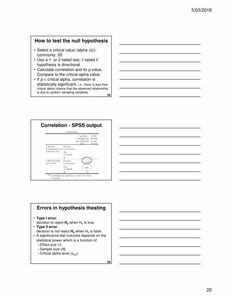
58
• Select a critical value (alpha (α));
commonly .05
• Use a 1- or 2-tailed test; 1-tailed if
hypothesis is directional
• Calculate correlation and its p value.
Compare to the critical alpha value.
• If p < critical alpha, correlation is
statistically significant, i.e., there is less than
critical alpha chance that the observed relationship
is due to random sampling variability.
How to test the null hypothesis
Correlation - SPSS output
60
• Type I error:
decision to reject H0 when H0 is true
• Type II error:
decision to not reject H0 when H0 is false
• A significance test outcome depends on the
statistical power which is a function of:
– Effect size (r)
– Sample size (N)– Critical alpha level (αcrit)
Errors in hypothesis thesting

5/03/2018
21
61
df critical(N - 2) p = .055
.67
10
.50
15
.41
20
.36
25
.32
30
.30
The higher the
N, the smaller
the correlation
required for a
statistically
significant result
– why?
Significance of correlation
Scatterplot showing a confidence
interval for a line of best fit
Image source: http://www.chriscorrea.com/2005/poverty-and-performance-on-the-naep/
Scatterplot showing a confidence
interval for a line of best fit
5/03/2018
22
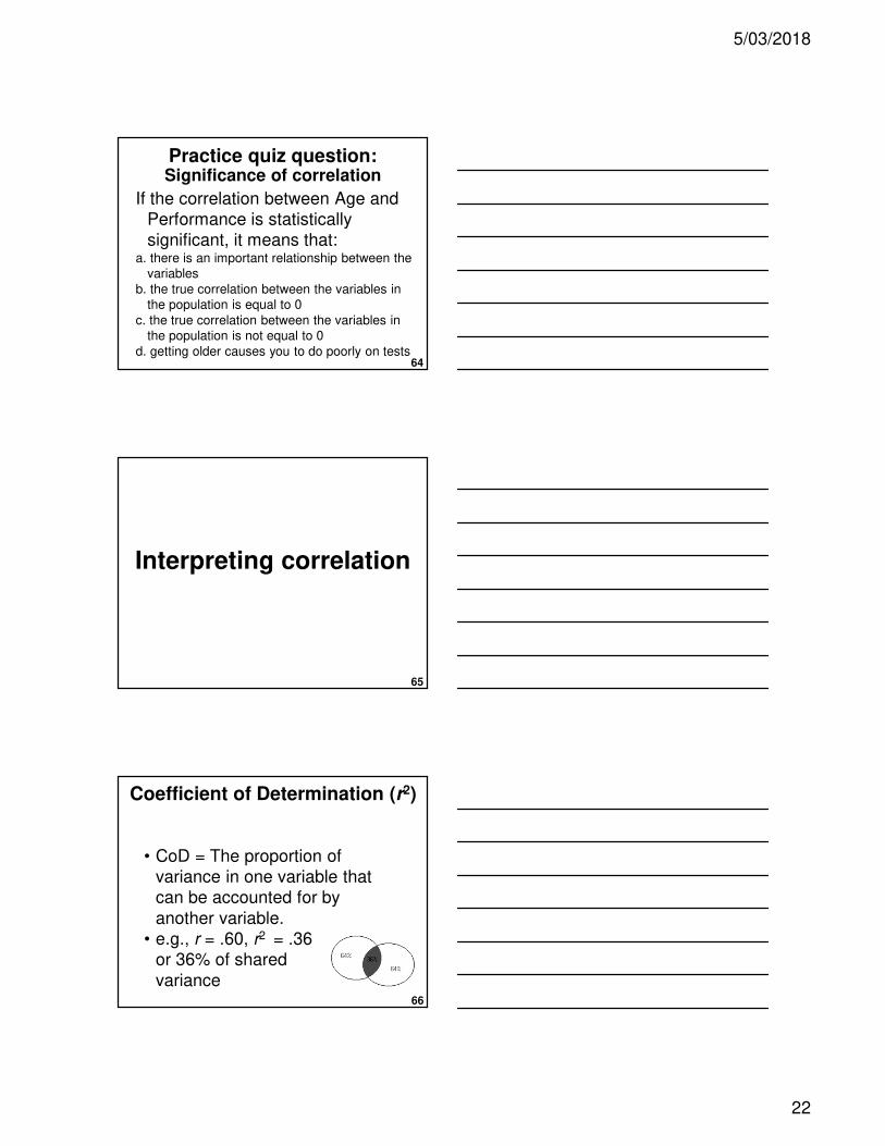
64
If the correlation between Age and
Performance is statistically
significant, it means that:a. there is an important relationship between the
variables
b. the true correlation between the variables in
the population is equal to 0
c. the true correlation between the variables in
the population is not equal to 0
d. getting older causes you to do poorly on tests
Significance of correlation Practice quiz question:
65
Interpreting correlation
66
• CoD = The proportion of
variance in one variable that
can be accounted for by
another variable.
• e.g., r = .60, r2 = .36
or 36% of shared
variance
Coefficient of Determination (r2)

5/03/2018
23
67
(Cohen, 1988)
• A correlation is an effect size• Rule of thumb:
Strength r
r2
Weak: .1 - .3 1 - 9%
Moderate: .3 - .5 10 - 25%
Strong: >.5 > 25%
Interpreting correlation
(Cohen, 1988)
WEAK (.1 - .3)
MODERATE (.3 - .5)
STRONG (> .5)
Size of correlation
69
(Evans, 1996)
Strength r r2
very weak .00 - .19 (0 to 4%)
weak .20 - .39 (4 to 16%)
moderate .40 - .59 (16 to
36%)
strong .60 - .79 (36% to 64%)
very strong .80 - 1.00 (64% to 100%)
Interpreting correlation

5/03/2018
24
Scale has no effect
on correlation.
Correlation of this scatterplot = -.9
Scale has no effect
on correlation.
Correlation of this scatterplot = -.9
a. -.5
b. -1
c. 0
d. .5
e. 1
What is the correlation of this scatterplot?

5/03/2018
25
a. -.5
b. -1
c. 0
d. .5
e. 1
What is the correlation of this scatterplot?
a. -.5
b. -1
c. 0
d. .5
e. 1
What is the correlation of this scatterplot?
75
“Number of children and marital satisfaction were inversely related (r (48) = -.35, p < .05), such that contentment in marriage tended to be lower for couples with more children. Number of children explained approximately 10% of the variance in marital satisfaction, a small-moderate effect.”
Write-up: Example

5/03/2018
26
76
(Pearson product-moment
linear correlation)
Assumptions and limitations
77
1 Levels of measurement
2 Normality
3 Linearity1 Effects of outliers
2 Non-linearity
4 Homoscedasticity
5 No range restriction
6 Homogenous samples
7 Correlation is not causation
8 Dealing with multiple correlations
Assumptions and limitations
78
• X and Y data should be sampled from
populations with normal distributions
• Do not overly rely on any single indicator
of normality; use histograms, skewness
and kurtosis (e.g., within -1 and +1)
• Inferential tests of normality (e.g.,
Shapiro-Wilks) are overly sensitive when
sample is large
Normality

5/03/2018
27
79
• Outliers can disproportionately
increase or decrease r.
• Options– compute r with & without outliers
– get more data for outlying values
– recode outliers as having more
conservative scores
– transformation
– recode variable into lower level of
measurement and a non-parametric
approach
Effects of outliers
(r = .63) Age and self-esteem
(outliers removed) r = .23
Age and self-esteem
5/03/2018
28
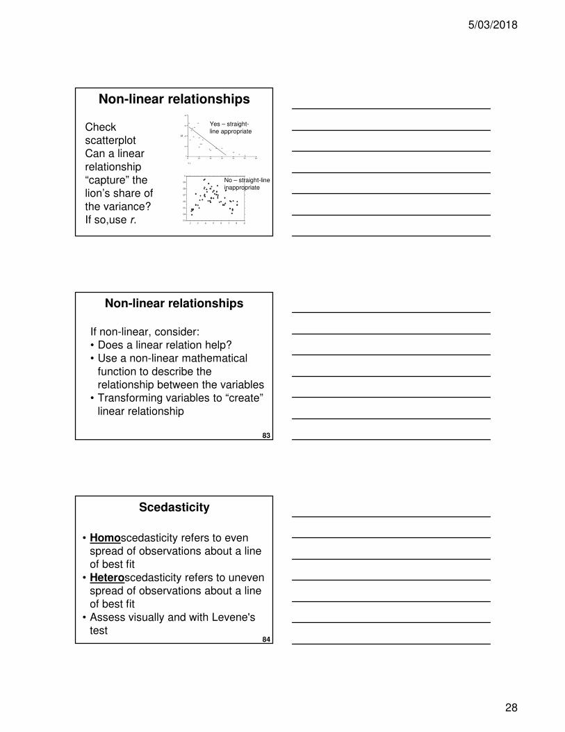
Check
scatterplot
Can a linear
relationship
“capture” the
lion’s share of
the variance?
If so,use r.
Yes – straight-
line appropriate
No – straight-line
inappropriate
Non-linear relationships
83
If non-linear, consider:
• Does a linear relation help?
• Use a non-linear mathematical
function to describe the
relationship between the variables
• Transforming variables to “create”
linear relationship
Non-linear relationships
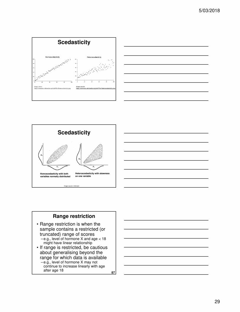
84
• Homoscedasticity refers to even
spread of observations about a line
of best fit
• Heteroscedasticity refers to uneven
spread of observations about a line
of best fit
• Assess visually and with Levene's
test
Scedasticity
5/03/2018
29
Image source:
https://commons.wikimedia.org/wiki/File:Homoscedasticity.png
Image source:
https://commons.wikimedia.org/wiki/File:Heteroscedasticity.png
Scedasticity
Image source: Unknown
Scedasticity
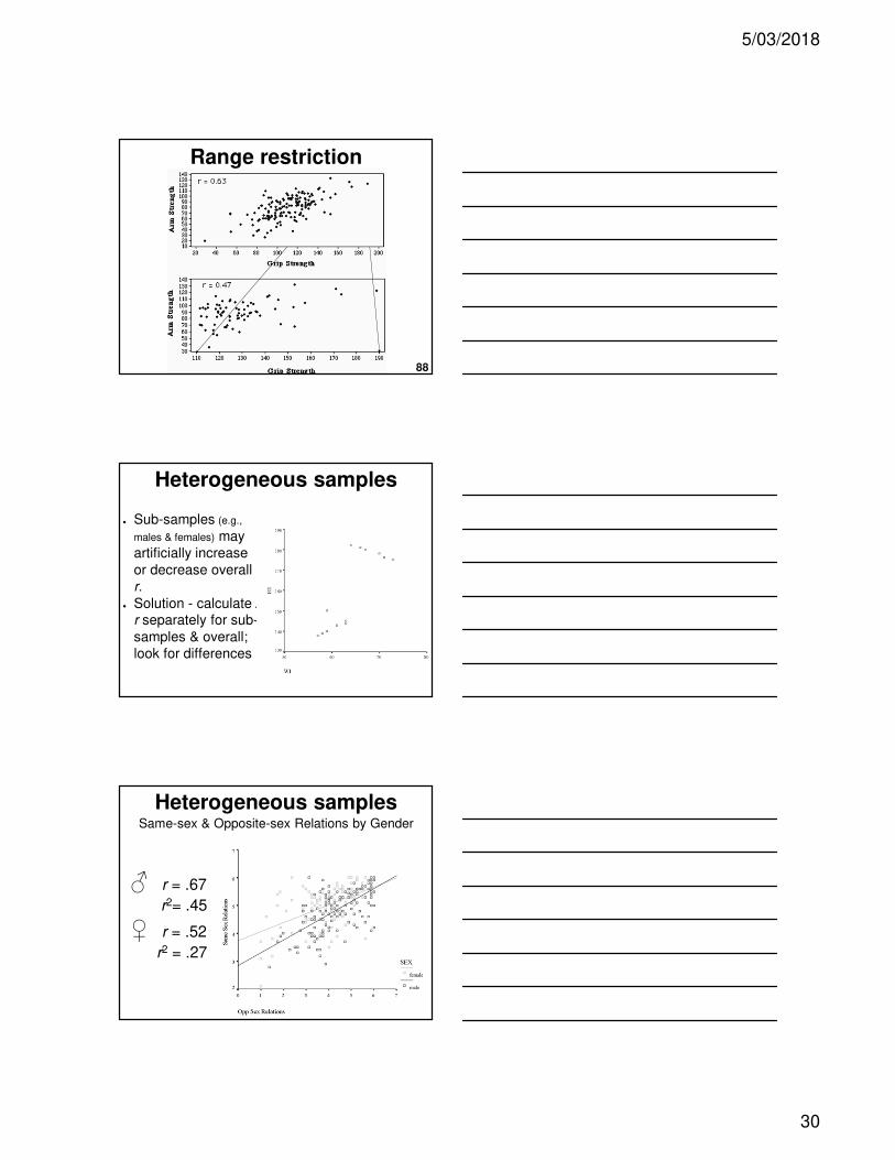
87
• Range restriction is when the sample contains a restricted (or truncated) range of scores– e.g., level of hormone X and age < 18
might have linear relationship
• If range is restricted, be cautious about generalising beyond the range for which data is available– e.g., level of hormone X may not
continue to increase linearly with age after age 18
Range restriction
5/03/2018
30
88
Range restriction
● Sub-samples (e.g.,
males & females) may
artificially increase
or decrease overall
r.
● Solution - calculate rr separately for sub-
samples & overall;
look for differences
Heterogeneous samples
Same-sex & Opposite-sex Relations by Gender
♂ r = .67
r2= .45
♀ r = .52
r2 = .27
Heterogeneous samples

5/03/2018
31
Weight and Self-esteem by Gender
♂ r = .50
♀r = -.48
Heterogeneous samples
e.g.,correlation between ice cream consumption and
crime, but actual cause is temperature
Image source: Unknown
Correlation is not causation
e.g., Stop global warming: Become a pirate
As the number of
pirates has reduced,
global temperature
has increased.
Image source: Unknown
Correlation is not causation

5/03/2018
32
Scatterplot matrices
organise scatterplots
and correlations
amongst several
variables at once.
However, they are not
sufficiently detailed for
more than about five
variables at a time.Image source: Unknown
Dealing with several correlations
Example of an APA Style
Correlation Table
Correlation matrix
96
Summary

5/03/2018
33
97
1 The world is made of covariations.
2 Covariations are the building blocks of
more complex multivariate
relationships.
3 Correlation is a standardised measure
of the covariance (extent to which two
phenomenon co-relate).
4Correlation does not prove
causation - may be opposite causality,
bi-directional, or due to other variables.
Summary: Correlation
98
The underlying purpose of
correlation is to help address the
question:What is the
• relationship or
• association or
• shared variance or
• co-relationbetween two variables?
Summary: Purpose of correlation
99
• Nominal by nominal:
Phi (Φ) / Cramer’s V, Chi-square
• Ordinal by ordinal:
Spearman’s rank / Kendall’s Tau b
• Dichotomous by interval/ratio:
Point bi-serial rpb
• Interval/ratio by interval/ratio:
Product-moment or Pearson’s r
Summary: Types of correlation

5/03/2018
34
100
1Choose correlation and graph type based on levels of measurement.
2Check graphs (e.g., scatterplot):– Linear or non-linear?
– Outliers?
– Homoscedasticity?
– Range restriction?
– Sub-samples to consider?
Summary: Correlation steps
101
3Consider– Effect size (e.g., Φ, Cramer's V, r, r2)
– Direction
– Inferential test (p)
4Interpret/Discuss– Relate back to hypothesis
– Size, direction, significance
– Limitations e.g.,
• Heterogeneity (sub-samples)
• Range restriction
• Causality?
Summary: Correlation steps
102
• Coefficient of determination
–Correlation squared
–Indicates % of shared variance
Strength r
r2
Weak: .1 - .3 1 – 10%
Moderate: .3 - .5 10 - 25%
Strong: > .5 >
25%
Summary:
Interpreting correlation

5/03/2018
35
103
1Levels of measurement
2Normality
3Linearity1 Effects of outliers
2 Non-linearity
4Homoscedasticity
5No range restriction
6Homogenous samples
7Correlation is not causation
Summary:
Assumptions & limitations
104
Evans, J. D. (1996). Straightforward statistics for the
behavioral sciences. Pacific Grove, CA: Brooks/Cole
Publishing.
Howell, D. C. (2007). Fundamental statistics for the
behavioral sciences. Belmont, CA: Wadsworth.
Howell, D. C. (2010). Statistical methods for
psychology (7th ed.). Belmont, CA: Wadsworth.
Howitt, D. & Cramer, D. (2011). Introduction to
statistics in psychology (5th ed.). Harlow, UK:
Pearson.
References
105
Exploratory factor analysis• Introduction to factor analysis
• Exploratory factor analysis examples
• EFA steps / process
Next lecture


