
Kreyszig by YHLee;100415; 6-1 Chapter 6. Laplace Transforms An ODE is reduced to an algebraic problem by operational calculus. The equation is solved by algebraic manipulation. The result is transformed back for the solution of ODE. 6.1 Laplace Transform. Inverse Transform. Linearity. s‐Shifting
A function ( )f t is defined for 0t ≥ .
Its Laplace transform is defined as
( ) ( ) ( )0
stF s f f t e dt∞
−= = ∫i
The inverse transform is defined as
( ) ( )1f t F−=i
Note
( ) ( )1 1, f f F F− −⎡ ⎤= =⎡ ⎤⎣ ⎦ ⎣ ⎦i i i i
Notation f is a function of t. F is a function of s.
Example 1 Laplace Transform Let ( ) 1f t = when 0t ≥ . Find ( )F s .
( ) ( )00
1 1st stF s f e dt ss s
∞∞− −= = ⇒ − ⇒∫i : s>0
Example 2 Laplace transform Let ( ) for 0atf t e t= ≥ . Find the Laplace transform.
( ) ( )0
0
1 s a tat at ste e e dt ea s
∞ ∞− −−= ⇒−∫i
When ( ) 0s a− >
( ) 1ates a
=−
i

Kreyszig by YHLee;100415; 6-2 Theorem 1 Linearity of the Laplace Transform
If ( ) ( ) ( ) ( ) and f t F s g t G s= =⎡ ⎤ ⎡ ⎤⎣ ⎦ ⎣ ⎦i i ,
then ( ) ( ) ( ) ( )+baf t bg t aF s G s+ =⎡ ⎤⎣ ⎦i
Proof:
( ) ( ) ( ) ( )
( ) ( )
( ) ( )
0
0 0
st
st st
af t bg t af t bg t e dt
a f t e dt b g t e dt
a f t b g t
∞−
∞ ∞− −
+ = +⎡ ⎤ ⎡ ⎤⎣ ⎦ ⎣ ⎦
= +
= +⎡ ⎤ ⎡ ⎤⎣ ⎦ ⎣ ⎦
∫
∫ ∫
i
i i
Example 3 Hyperbolic Functions Find the transforms of cosh and sinhat at .
[ ]
[ ]
2 2
2 2
1 1 1cosh
2 2
1 1 1sinh
2 2
at at
at at
e e sat
s a s a s a
e e aat
s a s a s a
−
−
⎡ ⎤+ ⎛ ⎞= = + =⎢ ⎥ ⎜ ⎟− + −⎝ ⎠⎣ ⎦⎡ ⎤− ⎛ ⎞= = − =⎢ ⎥ ⎜ ⎟− + −⎝ ⎠⎣ ⎦
i i
i i
Example 4 Cosine and Sine
Prove [ ] [ ]2 2 2 2cos , sin
st t
s sω
ω = ω =+ω +ω
i i
• By integrating by part
[ ] [ ]
[ ] [ ]
0 00
0 00
1cos cos cos sin sin ,
sin sin sin cos cos
stst st
stst st
et e t dt t e t dt t
s s s s
et e t dt t e t dt t
s s s
∞∞ ∞−− −
∞∞ ∞−− −
ω ωω = ω = ω − ω = − ω
−
ω ωω = ω = ω + ω = ω
−
∫ ∫
∫ ∫
i i
i i
→ [ ] [ ]
[ ] [ ]
1cos cos ,
1sin sin
t ts s s
t ts s s
ω ω⎛ ⎞ω = − ω⎜ ⎟⎝ ⎠
ω ω⎛ ⎞ω = ω⎜ ⎟⎝ ⎠
i i
i J i →
[ ]
[ ]
2 2
2 2
cos ,
sin
st
s
ts
ω =+ωω
ω =+ω
i
i
• By complex methods From the result of Example 2
2 2 2 2
1i t se i
s i s sω ω⎡ ⎤ = ⇒ +⎣ ⎦ − ω +ω +ω
i
From Euler formulas
[ ]ω⎡ ⎤ = ω + ω⎣ ⎦i i cos sini te t i t
→ [ ] [ ]2 2 2 2cos , sin
st t
s sω
ω = ω =+ω +ω
i i

Kreyszig by YHLee;100415; 6-3 Basic Transforms
• Proof of (4) We make the induction hypothesis that (4) holds for 0t ≥ .
1 1 1
00 0
1 1n st n st n st nnt e t dt e t e t dt
s s
∞∞ ∞+ − + − + −+⎡ ⎤ = = − +⎣ ⎦ ∫ ∫i
↑ ↑ =0 nt⎡ ⎤⎣ ⎦i
→ ( )12
1 !nn
nt
s+
+
+⎡ ⎤ =⎣ ⎦i
↑ It satisfies the induction hypothesis. So (4) is proved.
• Let’s prove (5)
1
0 0 0
1a
a st a x x aa
x dxt e t dt e e x dx
s s s
∞ ∞ ∞− − −
+
⎛ ⎞⎡ ⎤ = ⇒ ⇒⎜ ⎟⎣ ⎦ ⎝ ⎠∫ ∫ ∫i
↑ ↑ ≡st x ( )1aΓ + , gamma function

Kreyszig by YHLee;100415; 6-4 s‐Shifting: Replacing s by s‐a in the Transform Theorem 2 s‐Shifting
( ) ( )ate f t F s a⎡ ⎤ = −⎣ ⎦i
( ) ( )1ate f t F s a−= −⎡ ⎤⎣ ⎦i
Proof:
( ) ( ) ( )
0 0 0
st s a t st at atF s e f dt F s a e f dt e e f dt e f∞ ∞ ∞
− − − − ⎡ ⎤ ⎡ ⎤= → − = ⇒ ⇒⎣ ⎦ ⎣ ⎦∫ ∫ ∫ i
Example 5 s‐Shifting Prove 11 and 12 of the table 6.1
[ ]( )2 2 22
( )cos cosats s a
t e ts s a
−⎡ ⎤ω = → ω =⎣ ⎦ω + ω + −i i
[ ]( )2 2 22
sin sinatt e ts s a
ω ω⎡ ⎤ω = → ω =⎣ ⎦ω + ω + −i i
Find the inverse of
→ → Existence and Uniqueness of Laplace Transforms The growth restriction is defined as
( ) ktf t Me≤
f(t) is piecewise continuous if it is continuous and has finite limits in subintervals
Theorem 3 Existence Theorem for Laplace Transform
If f(t) is piecewise continuous satisfying the growth restriction for all 0t ≥ , then its Laplace transform exists for all s k> .
Proof: Since f(t) is piecewise continuous, ( )ste f t− is integrable.
Uniqueness If the Laplace transform of a given function exists, it is uniquely determined.

Kreyszig by YHLee;100415; 6-5 6.2 Transforms of Derivatives and Integrals. ODEs Theorem 1 Laplace Transform of Derivatives
[ ] [ ] ( )[ ] [ ] ( ) ( )2
' 0
" 0 ' 0
f s f f
f s f sf f
= −
= − −
i i
i i
The necessary condition: ' and "f f on the left side are piecewise continuous. and 'f f on the right side are continuous for all 0t ≥ satisfying the growth restriction.
Proof: Using integration by parts
↑ ↑ = [ ]fi
Using growth restriction
( ) ( ) 0 for st st kt s k t
t t te f t e Me e M s k− − − −
=∞ =∞ =∞≤ ⇒ ⇒ > .
Only left is ( ) ( )−
=⇒
00st
te f t f
→ [ ] [ ] ( )' 0f s f f= −i i
Similarly, using the first relation twice,
Theorem 2
If ( )1, ', ..., nf f f − is continuous for all 0t ≥ satisfying the growth restriction,
and ( )nf is piecewise continuous,
Example 2 Formula 7 and 8 in Table 6.1 Let ( ) cosf t t= ω
→ ( ) ( ) ( ) 20 1, ' 0 0, " cosf f f t t= = = −ω ω
Using the transform of a second derivative,
[ ] [ ] ( ) ( ) [ ]2 2" 0 ' 0f s f sf f s f s= − − ⇒ −i i i → [ ] 2 2
sf
s=ω +
i
↑ = [ ]2 f−ω i
Similarly, ( ) ( )sin , 0 0, ' cosg t g g t t= ω = = ω ω
[ ] [ ]'g s g=i i → [ ] [ ] 2 2cosg t
s sω ω
= ω ⇒ω +
i i
↑ = [ ]cos tω ωi

Kreyszig by YHLee;100415; 6-6 Laplace Transform of the Integral of a Function Theorem 3 Laplace Transform of Integra
If Laplace transform of f(t) is given as F(s), for s>0, s>k and t>0
( ) ( )0
1t
f d F ss
⎡ ⎤τ τ =⎢ ⎥
⎣ ⎦∫i and ( ) ( )1
0
1t
f d F ss
− ⎡ ⎤τ τ = ⎢ ⎥⎣ ⎦∫ i
Proof: Let
( ) ( )0
t
g t f d= τ τ∫
Then
Since f(t) is piecewise continuous, g(t) is continuous and satisfies the growth restriction.
Example 3
Find the inverse of ( ) ( )2 2 2 2 2
1 1 and
s s s s+ω +ω.
Using (8) of Table 6.1
12 2
1 sin ts
− ω⎡ ⎤ =⎢ ⎥ ω+ω⎣ ⎦i
Using Theorem 3
( )12 2 2
0
1 1 sin 11 cos
t
d ts s
− ⎡ ⎤ ωτ⎛ ⎞ = τ⇒ − ω⎜ ⎟⎢ ⎥ ω+ω ω⎝ ⎠⎣ ⎦∫i
Using Theorem 3 again
( )12 2 2 2 2 3
0
1 1 1 sin1 cos
t t td
s s− ⎡ ⎤ ω⎛ ⎞ = − ωτ τ⇒ −⎜ ⎟⎢ ⎥+ω ω ω ω⎝ ⎠⎣ ⎦
∫i

Kreyszig by YHLee;100415; 6-7 Differential Equations, Initial Value Problems ODEs can be solved by Laplace transform method. An initial value problem ( )" 'y ay by r t+ + = ( ) ( ) 10 , ' 0oy K y K= =
r(t) is input and y(t) is output. Step 1 Setting up the subsidiary equation The Laplace transform of the ODE
( ) ( ) ( )2 0 ' 0 0s Y sy y a sY y bY R⎡ ⎤− − + − + =⎡ ⎤⎣ ⎦⎣ ⎦ : [ ] ( ) [ ] ( ), y Y s r R s= =i i
→ ( ) ( ) ( ) ( )2 0 ' 0s as b Y s a y y R+ + = + + + : subsidiary equation
Step 2 Solve the subsidiary equation by algebra
( ) ( ) ( )0 ' 0Y s a y y Q RQ= + + +⎡ ⎤⎣ ⎦
where
( ) ( ) 222
1 1
1 12 4
Q ss as b
s a b a
= ⇒+ + ⎛ ⎞+ + −⎜ ⎟
⎝ ⎠
: transfer function
Note, if ( ) ( )0 ' 0 0y y= =
[ ][ ]output
inputY
QR
= =i
i
Step 3 Inversion of Y for y Example 4 Initial value problem Solve
Find the subsidiary equation
→ → ↑ Use partial fraction expansion →

Kreyszig by YHLee;100415; 6-8 Example 5 Comparison with the usual method Solve
Find the subsidiary equation
The solution
( )
( ) ( )( )
( ) ( ) ( ) ( )351 142 2
2 2 2352 2 235 35 351 1 142 4 2 4 2 4
0.16 0.08 0.080.16
s s
s s s
+ + +⇒ ⇒ +
+ + + + + +
Use shifting theorem and formulas for cosine and sine.
( ) [ ] ( ) ( )/2 35 354 435
4
0.080.16 cos cos ty t Y e t t−= = +i
Advantage of the Laplace Method
1. Nonhomogeneous ODE can be solved without solving the homogeneous ODE. 2. Initial values are automatically taken care of. 3. Complicated input r(t) can be handled very efficiently.
Example 6 Shifted Data Problem The initial conditions do not start at t=0
( ) ( )" 2 y / 4 / 2, y' / 4 2 2y y t+ = π = π π = −
We set / 4t t= + π
( ) ( ) ( )/ 4y t y t y t= + π = , ( ) ( ) ( )
= = = 'dy t dy tdy t dt
ydt dt dt dt
The ODE becomes
( ) ( )" 2( / 4) y 0 / 2, y' 0 2 2y y t t t+ = + π = = π = = −
The subsidiary equation
( )22
2 / 22 2
2s Y s Y
ssπ π
− − − + = +
Solve for Y
Partial fraction expansion
2 2 2 2 2 2 2
2 2 / 2 / 2 / 2 2 2 2 / 2 21 1 1 1 1
s sY
s ss s s s s s s− − π π π − π −
= + + + + + ⇒ + ++ + + + +
→ 2 / 2 2siny t t= + π −
→ 2 2sin( / 4)y t t= − − π

Kreyszig by YHLee;100415; 6-9
6.3 Unit Step Function. t‐shifting
The unit step function or Heaviside function is defined as
( ) 0 if
1 if
u t a t a
t a
− = <
= >
The Laplace transform
( ) ( )0
stst st
a t a
eu t a e u t a dt e dt
s
∞∞ ∞ −− −
=
− = − = = −⎡ ⎤⎣ ⎦ ∫ ∫i
( )ase
u t as
−
− =⎡ ⎤⎣ ⎦i
Let ( ) 0f t = for t < 0.
Then ( ) ( )f t a u t a− − is ( )f t shifted to the right by the amount of a.

Kreyszig by YHLee;100415; 6-10 Time Shifting (t‐shifting): Replace t by t‐a in f(t) Theorem 1 t‐Shifting
F(s) is the transform of f(t) The shifted function is given as
( ) ( )
( )− − = <
= − >
0 if
if
f t a u t a t a
f t a t a
Its Laplace transform is
( ) ( ) ( )asf t a u t a e F s−− − =⎡ ⎤⎣ ⎦i
Proof:
Let a tτ + =
↑ The lower limit is changed Example 1 Use of Unit Step Function Write f(t) using unit step function and find its transform
Using unit step functions
Perform the transform after writing terms as ( ) ( )f t a u t a− −
→
• You might have used ( ) ( ) ( )asf t u t a e f t a−− = +⎡ ⎤ ⎡ ⎤⎣ ⎦ ⎣ ⎦i i

Kreyszig by YHLee;100415; 6-11
( ) ( ) ( )/
1 /as bsoV R
I s e es RC
− −⎡ ⎤= −⎢ ⎥
+⎢ ⎥⎣ ⎦
Example 2 Application of Both Shifting Theorems Find the inversion of
Without the exponential functions at the numerator, F(s) would be
21 1sin , sin , tt t te−π π
π π
Next, the exponential functions mean t‐shifting,
→ ( ) ( ) ( ) ( ) ( ) ( ) ( ) ( )2 31 1sin 1 1 sin 2 2 3 3tf t t u t t u t t e u t− −= π − − + π − − + − −⎡ ⎤ ⎡ ⎤⎣ ⎦ ⎣ ⎦π π
Example 3 RC‐Circuits Find i(t) if a single rectangular wave with voltage Vo is applied. The circuit was quiescent before the wave is applied.
The input voltage is
( ) ( )oV u t a u t b− − −⎡ ⎤⎣ ⎦
The circuit is modeled by the integro‐differential equation
The subsidiary eq. :
→ ( ) ( ) ( ) ( ) ( )( )/ ( )/t a RC t b RCoVi t e u t a e u t bR
− − − −⎡ ⎤= − − −⎣ ⎦ Solve for I(s) :
↑
( )/t RCoV eR
−⎡ ⎤⎣ ⎦i

Kreyszig by YHLee;100415; 6-12 Example 4 RLC circuit with a sinusoidal input The input is given by a sinusoidal function only for a short time interval.
The current and charge are initially zero.
The model for i(t)
The subsidiary equation
( )22 2
4000.1 11 100 100 1
400sI
sI I es s
− π+ + = −+
Solve for I
( )( )( )( )
2 21 22 2 2 2 2
10 400 1000 400100 1 1
110 1000 400 10 100 400s ss s
I e e I Is s s s s s
− π − π⋅ ⎡ ⎤= − ⇒ − ≡ −⎣ ⎦+ + + + + +
Partial fraction expansion
Constants A, B, D, K are found as follows. After multiplication by the common denominator,
Insert s=‐10 → A=‐0.27760 Insert s=‐100 → B=2.6144 Collect 3s terms → 0=A+B+D → D=‐2.3368 Collect 2s terms → 0=100A+10B+110D+k → K=258.66 Then
→ ( )2i t can be obtained using t‐shifting
( ) ( ) ( ) { } { } ( )10 2 100 22 0.2776 2.6144 2.3368cos 400( 2 ) 0.6467sin 400( 2 ) 2t ti t e e t t u t− − π − − π⎡ ⎤= − + − − π + − π − π⎣ ⎦
The final solution is ( ) ( ) ( )1 2i t i t i t= −

Kreyszig by YHLee;100415; 6-13 6.4 Short Impulses. Dirac Delta Function. Partial Fraction
Dirac delta function or unit impulse function is defined as
( ) if
0 otherwise
t a t aδ − = ∞ =
=
( ) 1a
a
t a dt+ε
−ε
δ − =∫
The delta function can be obtained by taking the limit of kf
( ) ( )0
lim kkt a f t a
→δ − = −
Sifting property of delta function
( ) ( ) ( )a
a
g t t a dt g a+ε
−ε
δ − =∫
The Laplace transform of delta function. Start from kf
( ) ( ) ( ){ }1kf t a u t a u t a k
k⎡ ⎤− = − − − +⎣ ⎦
→ Take the limit 0k→ and apply l’Hopital’s rule to the quotient.
0 0
1lim lim
ks ksas as
k k
e see e
ks s
− −− −
→ →
⎡ ⎤ ⎡ ⎤−⇒⎢ ⎥ ⎢ ⎥
⎣ ⎦ ⎣ ⎦
→ ( ) ast a e−δ − =⎡ ⎤⎣ ⎦i

Kreyszig by YHLee;100415; 6-14 Example 1 Mass‐Spring system under a square wave Input is of the form of a rectangular function
The subsidiary equation
Use the partial fraction expansion : The inverse transform : Using t‐shifting
( ) ( ) ( ) ( ) ( ) ( ) ( )1 2 1 2 2 21 1 1 11 2
2 2 2 2t t t ty t e e u t e e u t− − − − − − − −⎡ ⎤ ⎡ ⎤= − + − − − + −⎢ ⎥ ⎢ ⎥⎣ ⎦ ⎣ ⎦
Example 2 Hammer blow response of a mass‐spring system The input is given by a delta function
Solving algebraically
The solution ( ) ( ) ( )( 1) 2( 1)1 1t ty t e u t e u t− − − −= − − −

Kreyszig by YHLee;100415; 6-15 Example 3 Four‐Terminal RLC‐Network Find the output voltage if 420 , 1 , 10R L H C F−= Ω = = . The input is a delta function and current and charge are zero at t=0.
The voltage drops on R, L, C should be equal to the input. Using 'i q=
The subsidiary equation
Using s‐shifting and 29900 99.50≈
The solution
More on Partial Fractions
The solution of a subsidiary equation is of the form ( )( )
F sY
G s=
Partial fraction representation may be needed.
(1) Unrepeated factor (s‐a) in G(s) → Partial fraction should be ( )
As a−
(2) Repeated factor ( )2s a− in G(s) → Partial fractions ( ) ( )2
A Bs as a
+−−
Repeated factor ( )3s a− in G(s) → Partial fractions ( ) ( ) ( )3 2
A B Cs as a s a
+ +−− −
(3) Unrepeated complex factors ( )2 2s⎡ ⎤−α +β⎣ ⎦ → Partial fraction ( )2 2
As B
s
+⎡ ⎤−α +β⎣ ⎦
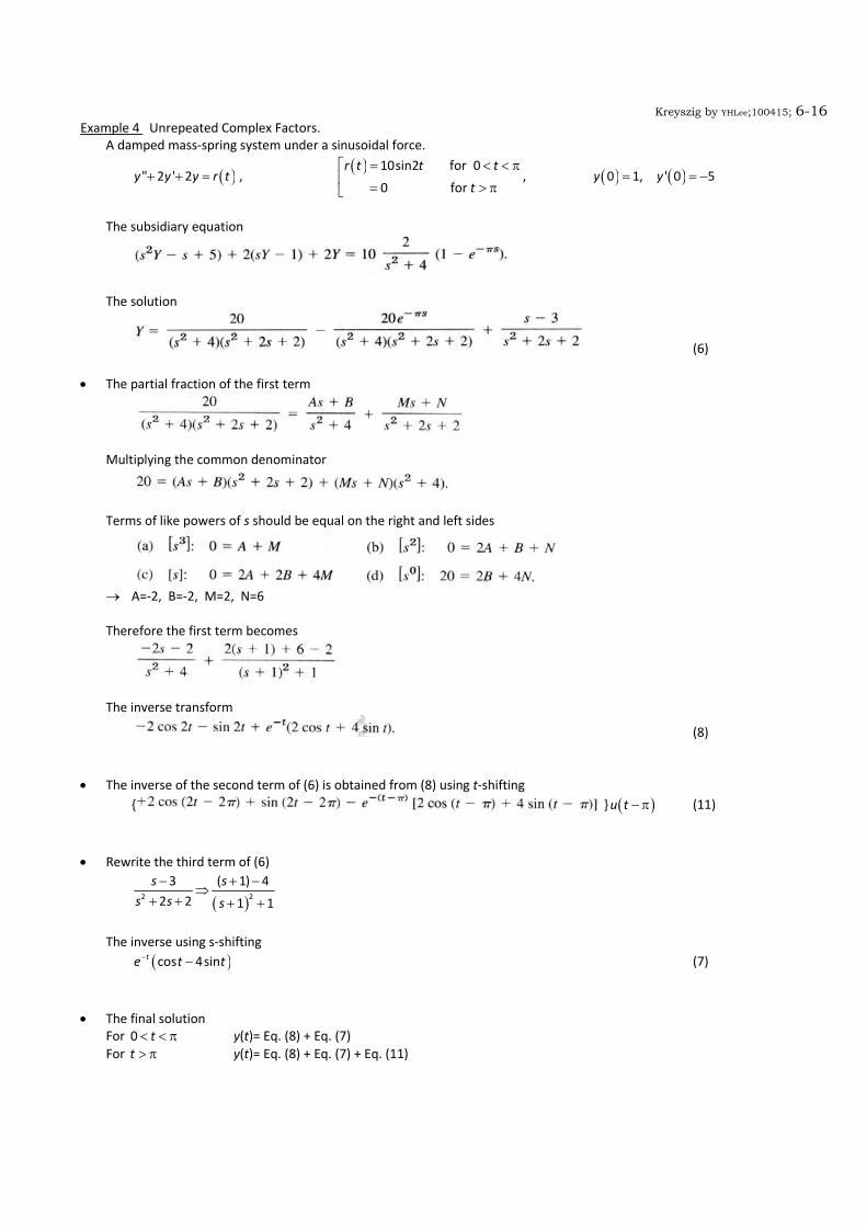
Kreyszig by YHLee;100415; 6-16 Example 4 Unrepeated Complex Factors. A damped mass‐spring system under a sinusoidal force.
( )" 2 ' 2y y y r t+ + = , ( ) 10sin2 for 0
0 for
r t t t
t
⎡ = < < π⎢
= > π⎣, ( ) ( )0 1, ' 0 5y y= = −
The subsidiary equation
The solution
(6) • The partial fraction of the first term
Multiplying the common denominator
Terms of like powers of s should be equal on the right and left sides
→ A=‐2, B=‐2, M=2, N=6 Therefore the first term becomes
The inverse transform
(8)
• The inverse of the second term of (6) is obtained from (8) using t‐shifting { } ( )u t − π (11)
• Rewrite the third term of (6)
( )2 2
3 ( 1) 4
2 2 1 1
s ss s s
− + −⇒
+ + + +
The inverse using s‐shifting ( )cos 4sinte t t− − (7)
• The final solution For 0 t< < π y(t)= Eq. (8) + Eq. (7) For t > π y(t)= Eq. (8) + Eq. (7) + Eq. (11)

Kreyszig by YHLee;100415; 6-17 6.5 Convolution. Integral Equations
The convolution of two functions f and g is defined as
( ) ( ) ( )0
*t
f g f g t d≡ τ − τ τ∫ : Note the integration interval
Theorem 1 Convolution theorem
If F and G are Laplace transforms of f and g, respectively, the multiplication FG is the Laplace transform of the convolution (f*g)
Proof:
Set p t= − τ , then
Calculate the multiplication
↑ ↑ ↑ G can be inside of F For fixed τ , integrate from τ to ∞ . because and t τ are independent. ( The integration over blue region ) The integration can be changed as
• Some properties of convolution
( )0
*ste f g dt∞
−⇒ ∫

Kreyszig by YHLee;100415; 6-18 Example 1 Convolution
Let ( ) ( )1
H ss a s
=−
. Find h(t).
Rearrange : ( ) ( )1 1
H ss a s
⎛ ⎞= ⎜ ⎟− ⎝ ⎠
↑ ↑ F(s) G(s) Inverse transforms : ( ) ( ), 1atf t e g t= =
Using convolution theorem : ( ) ( ) ( ) ( )0
1* 1 1
ta ath t f t g t e d e
aτ= ⇒ ⋅ τ⇒ −∫
Example 2 Convolution
Let ( )( )22 2
1H s
s=
+ω. Find h(t).
Rearrange : ( )( ) ( ) ( )2 2 2 2 22 2
1 1 1H s
s ss= ⇒
+ω +ω+ω
Inverse of ( )2 2
1
s +ω :
sin tωω
Using convolution theorem : ( ) ( )2 20
sin sin 1 1 sin* sin sin cos
2
tt t th t t d t t
ω ω ω⎛ ⎞ ⎡ ⎤= ⇒ ωτ ω − τ τ⇒ − ω +⎜ ⎟ ⎢ ⎥ω ω ωω ω⎝ ⎠ ⎣ ⎦∫
Example 3 Unusual Properties of Convolution *1f f≠ in general → ( )* 0f f ≥ may not hold →
Applications to Nonhomogeneous Linear ODEs Nonhomogeneous linear ODE in standard form ( )" 'y ay by r t+ + = : a and b, constant
The solution
( ) ( ) ( ) ( ) ( ) ( ) ( )0 ' 0Y s s a y y Q s R s Q s= + + +⎡ ⎤⎣ ⎦ : ( ) 2
1Q s
s as b=
+ +, transfer function
The inverse of the first right term can be easily obtained. The inverse of the second term, assuming ( ) ( )0 ' 0 0y y= =
( ) ( ) ( )0
t
y t q t r d= − τ τ τ∫
The output is given by the convolution of the impulse response q(t) and the driving force r(t).

Kreyszig by YHLee;100415; 6-19 Example 5 Mass‐spring system Solve
( )" 3 ' 2y y y r t+ + = , ( ) 1 for 1 2
0 otherwise
r t t⎡ = < <⎢
=⎣ ( ) ( )0 ' 0 0y y= =
The transfer function
Its inverse
Since ( ) ( )0 ' 0 0y y= = , the solution is given by the convolution of q and r.
( ) ( ) ( ) ( ) ( ) ( ) ( ) ( ) ( ) ( )2 212
10 0 1
1 2t t t t
t t t ty t q t r d q t u u d e e d e eτ=
− −τ − −τ − −τ − −τ
τ=⎡ ⎤ ⎡ ⎤= − τ τ τ⇒ − τ τ − − τ − τ⇒ − τ⇒ −⎡ ⎤⎣ ⎦ ⎣ ⎦ ⎣ ⎦∫ ∫ ∫i i
↑ ↑ r(t)=1 only for 1<t<2 Note the change in the lower limit. t should be less than 2. For t<1 : y(t) = 0
For 1<t<2 : The upper limit is t, ( ) ( ) ( ) ( ) ( )2 1 2 112
1
1 12 2
tt t t ty t e e e e
τ=− −τ − −τ − − − −
τ=⎡ ⎤= − ⇒ − +⎣ ⎦
For t>2 : The upper limit is 2, ( ) ( ) ( ) ( ) ( ) ( ) ( )22 2 2 2 1 2 11
21
1 12 2
t t t t t ty t e e e e e eτ=
− −τ − −τ − − − − − − − −
τ=
⎡ ⎤⎡ ⎤= − ⇒ − − −⎢ ⎥⎣ ⎦ ⎣ ⎦
Integral Equations Convolutions can be used to solve certain integral equations Example 6 A volterra Integrals Equation of the Second Kind Solve
↑ Convolution of ( ) ( ) and siny t t
Using the convolution theorem we obtain the subsidiary equation
( ) ( ) ( )2
2 2 2
1 11 1
sY s Y s Y s
s s s− = ⇒
+ + → ( )
2
4 2 4
1 1 1sY s
s s s+
= ⇒ +
The answer is

Kreyszig by YHLee;100415; 6-20 6.6 Differentiation and Integration of Transforms. Differentiation of Transforms If F(s) is the transform of f(t), then its derivative is
( ) ( )0
stF s f t e dt∞
−= ∫ → ( ) ( ) ( )0
' stdF sF s t f t e dt
ds
∞−= = −∫
Consequently
( ) ( )'t f t F s= −⎡ ⎤⎣ ⎦i and ( ) ( )1 'F s t f t− = −⎡ ⎤⎣ ⎦i
Example 1 Differentiation of Transforms The table can be proved using differentiation of F(s).
The second one
[ ]( )2 2 22 2
2sin
sdt t
ds s s
β⎡ ⎤ββ = − ⇒⎢ ⎥+β⎣ ⎦ +β
i
Integration of Transforms If f(t) has a transform and ( )
0lim /t
f t t→ +
⎡ ⎤⎣ ⎦ exists,
( ) ( )
s
f tF s ds
t
∞⎡ ⎤=⎢ ⎥
⎣ ⎦∫i and ( ) ( )1
s
f tF s ds
t
∞− ⎡ ⎤
=⎢ ⎥⎣ ⎦∫i
Proof: From the definition
( ) ( ) ( ) ( )0 0
st st
s s s
f tF s ds e f t dt ds f t e ds dt
t
∞ ∞ ∞ ∞ ∞− −⎡ ⎤ ⎡ ⎤ ⎡ ⎤
= ⇒ ⇒⎢ ⎥ ⎢ ⎥ ⎢ ⎥⎣ ⎦⎣ ⎦ ⎣ ⎦
∫ ∫ ∫ ∫ ∫ i
↑ ↑ Reverse the order of integration. = /ste t−

Kreyszig by YHLee;100415; 6-21 Example 2 Differentiation and Integration of Transforms Find the inverse transform of F(s) = Its derivative
Take the inverse transform
( ) ( )1 12 2
2 2' 2cos 2
sF s t t f t
ss− − ⎡ ⎤⇒ − ⇒ ω − = −⎡ ⎤⎣ ⎦ ⎢ ⎥+ ω⎣ ⎦
i i
→ ( ) 2cos 2tf t
tω −
= −
• Using integration of transforms Let → Then
( ) ( ) ( ) ( )' 0s s
F s F F s ds G s ds∞ ∞
= ∞ − ⇒ −∫ ∫
Take the inverse transform of both sides
( ) ( )g tf t
t= − ( ) ( )2 cos 1
t
f tt
ω −→ = −
Special Linear ODEs with Variable Coefficients Use differentiation of transform to solve ODEs. Let [ ]y Y=i → [ ] ( )' 0y sY y= −i .
Using differentiation of transform
[ ] ( )' 0d dY
ty sY y Y sds ds
= − − ⇒ − −⎡ ⎤⎣ ⎦i
Similarly, using [ ] ( ) ( )2" 0 ' 0y s Y sy y= − −i
[ ] ( ) ( ) ( )2 2" 0 ' 0 2 0d dY
ty s Y sy y sY s yds ds
⎡ ⎤= − − − ⇒ − − +⎣ ⎦i

Kreyszig by YHLee;100415; 6-22 Example 3 Laguerre’s Equation Laguerre’s ODE is ( )" 1 ' 0ty t y ny+ − + = n=0, 1, 2, …
The subsidiary equation
→ Separating variables, using partial fractions
2
1 11
dY n s n nds ds
Y s ss s+ − +⎛ ⎞= − ⇒ −⎜ ⎟−− ⎝ ⎠
→ ( ) ( ) ( )1
1ln ln 1 1 ln ln
n
n
sY n s n s
s +
−= − − + ⇒ →
( )1
1n
n
sY
s +
−=
The inverse transform is given by Rodrigues’s formula [ ]1
nl Y−=i
→ n=1, 2, … • Prove Rodrigues’s formula Using s‐shifting
Using the n‐th derivative of f,
After another s‐shifting

Kreyszig by YHLee;100415; 6-23 6.7 Systems of ODEs
The Laplace transform can be used to solve systems of ODEs. Consider a first‐order linear system with constant coefficients
The subsidiary equations
Rearrange
( ) ( ) ( )
( ) ( ) ( )11 1 12 2 1 1
21 1 22 2 2 2
0
0
a s Y a Y y G s
a Y a s Y y G s
− + = − −
+ − = − −
Solve this system algebraically for ( ) ( )1 2 and Y s Y s and take the inverse transform for ( ) ( )1 2 and y t y t
Example 2 Electrical Network Find the currents ( ) ( )1 2 and i t i t .
( ) 100 only for 0 0.5v t volts t= ≤ ≤ and ( ) ( )0 = ' 0 0i i =
From Kirchhoff’s voltage law in the lower and the upper circuits,
Rearrange
The subsidiary equations using ( ) ( )1 20 = 0 0i i =
Solve algebraically for 1 2 and I I
( )( )( ) ( ) ( ) ( ) ( )
( )( ) ( ) ( ) ( ) ( )
/2 /21 1 7 1 7
2 2 2 2
/2 /21 1 7 1 7
2 2 2 2
125 1 500 125 6251 1
7 3 21
125 500 250 2501 1
7 3 21
s s
s s
sI e e
s s s s s s
I e es s s s s s
− −
− −
⎡ ⎤+= − ⇒ − − −⎢ ⎥
+ + + +⎢ ⎥⎣ ⎦⎡ ⎤
= − ⇒ − + −⎢ ⎥+ + + +⎢ ⎥⎣ ⎦

Kreyszig by YHLee;100415; 6-24 The inverse transform of the square bracket terms using s‐shifting.
/2 7 /2
/2 7 /2
500 125 6257 3 21500 250 2507 3 21
t t
t t
e e
e e
− −
− −
− −
− +
Using t‐shifting
( ) ( )
( ) ( )
/2 7 /2 ( 0.5)/2 7( 0.5)/21
/2 7 /2 ( 0.5)/2 7( 0.5)/22
500 125 625 500 125 6250.5
7 3 21 7 3 21
500 250 250 500 250 2500.5
7 3 21 7 3 21
t t t t
t t t t
i t e e e e u t
i t e e e e u t
− − − − − −
− − − − − −
⎧ ⎫ ⎧ ⎫= − − − − − −⎨ ⎬ ⎨ ⎬⎩ ⎭ ⎩ ⎭⎧ ⎫ ⎧ ⎫= − + − − + −⎨ ⎬ ⎨ ⎬⎩ ⎭ ⎩ ⎭
Note that the solution for 1
2t ≥ is different from that for 120 t≤ ≤ due to the unit step function.
Example 3 Two masses on Springs Ignoring the mass of the springs and the damping
↑ ↑ ↑ Newton’s second law(mass X acceleration) ↑ ↑ Hooke’s law (restoring force) Initial conditions
( ) ( )( ) ( )
1 2
1 2
0 0 1
' 0 3 , ' 0 3
y y
y k y k
= =
= = −
The subsidiary equations
The algebraic solution using Cramer’s rule
The final solution
→
![[Kreyszig] Matematicas Avanzadas Para Ingeneria](https://cdn.vdocuments.mx/doc/165x107/563db921550346aa9a9a50c6/kreyszig-matematicas-avanzadas-para-ingeneria.jpg)


