J o u r n a l o f E c o n o m i c C o o p e r a t i o n
& Development
J o u r n a l o f E c o n o m i c C o o p e r a t i o n
& Development
Stat i s t ica l Economic and Socia l Research
and Training Centre for Islamic Countries
(SESRIC)
Journ
al of Econ
omic C
ooperation
and
Develop
men
t
Se
pte
mb
er 2016
VO
LU
ME
37, N
o.3
ISSN 1308 - 7800 Volume 37, No. 3 September 2016ISSN 1308 - 7800 Volume 37, No. 3 September 2016
Oil Price Effects on Exchange Rate, Output and Consumer Price: A Case Study of Small Open Economy of Oman
The Impacts of Foreign Labour Entry on the Labour Productivity in the Malaysian Manufacturing Sector
The Real Effect of Government Debt: Evidence from the Malaysian Economy
Environmental Kuznets Curve for Deforestation in Indonesia: An ARDL Bounds Testing Approach
Determination of the Degree of Development and the Impact of the Information Environment on the Formation of A System of Social Control in Procurement Under the Russian Contract System (Method of Content Analysis of Information Resources on the Internet)
Bilateral Trade through Official Channel between India and Bangladesh: An Analysis with the Use of Time Series Forecasting Models
Ahmed Nawaz Hakro and Abdallah Mohammed Omezzine
Nur Sabrina Mohd Palel, Rahmah Ismail and Abdul Hair Awang
Siti Nurazira Mohd Daud
Efendi Agus Waluyo and Taku Terawaki
N.A. Mamedova and A.N. Baykova
Muhammad Mahboob Ali and Anita Medhekar
CMYK
CMYK
STATISTICAL, ECONOMIC AND SOCIAL RESEARCHAND TRAINING CENTRE FOR ISLAMIC COUNTRIES
Kudüs Cad. No:9 Diplomatik Site 06450 ORAN-Ankara, TurkeyTel: (90-312) 468 61 72-76 Fax: (90-312) 468 57 26
Email: [email protected] Web: www.sesric.org
STATISTICAL, ECONOMIC AND SOCIAL RESEARCHAND TRAINING CENTRE FOR ISLAMIC COUNTRIES
Kudüs Cad. No:9 Diplomatik Site 06450 ORAN-Ankara, TurkeyTel: (90-312) 468 61 72-76 Fax: (90-312) 468 57 26
Email: [email protected] Web: www.sesric.org

ISSN 1308 – 7800 Volume 37, No.3, September 2016
J o u r n a l o f
E c o n o m i c C o o p e r a t i o n
& D e v e l o p m e n t
Statistical Economic and Social Research
and Training Centre for Islamic Countries
(SESRIC)


Contents
Ahmed Nawaz Hakro and Abdallah Mohammed Omezzine
Oil Price Effects on Exchange Rate, Output and Consumer Price:
A Case Study of Small Open Economy of Oman .................................... 1
Nur Sabrina Mohd Palel, Rahmah Ismail and Abdul Hair Awang
The Impacts of Foreign Labour Entry on the Labour Productivity in the
Malaysian Manufacturing Sector ........................................................... 29
Siti Nurazira Mohd Daud
The Real Effect of Government Debt: Evidence from the Malaysian
Economy ................................................................................................. 57
Efendi Agus Waluyo and Taku Terawaki
Environmental Kuznets Curve for Deforestation in Indonesia:
An ARDL Bounds Testing Approach .................................................... 87
N.A. Mamedova and A.N. Baykova
Determination of the Degree of Development and the Impact of the
Information Environment on the Formation of A System of Social
Control in Procurement Under the Russian Contract System (Method of
Content Analysis of Information Resources on the Internet)............... 109
Muhammad Mahboob Ali and Anita Medhekar
Bilateral Trade through Official Channel between India and Bangladesh:
An Analysis with the Use of Time Series Forecasting Models ........... 135


EDITORIAL NOTE
While many developed and developing countries are still suffering the
negative impact of the global economic and financial crisis in terms of
continuous slowdown of economic growth and high unemployment rates,
the development of various sectors at international, regional and national
levels seems to be still struggling.
In this current issue of the Journal of Economic Cooperation and
Development – September 2016, six valuable articles have been selected
that analyse global oil prices, the importance of labour productivity in the
manufacturing sector, the relationship between government debt and
economic growth, deforestation rates, social control in procurement, and
bilateral trade and focus on trends in some Asian countries such as
Bangladesh, India, Indonesia, Malaysia, Oman and Russia.
The first article examines and explores the sharp fluctuations in global oil
prices and their associated impact on global economic imbalances which
have contributed to the renewed debate among the policy makers regarding
the nature and extent of these fluctuations. It also investigates the impact of
oil prices on the small open economy of Oman.
The second article emphasizes that the improvement and strengthening of
labour productivity has become an important approach to accelerate the
growth of the manufacturing sector in Malaysia. It also attempts to analyse
the impacts of the entry of foreign workers on the labour productivity of the
manufacturing sector in Malaysia stressing the fact that the contribution of
foreign labour on labour productivity is smaller compared to the local
labour.
The third article investigates the real effect of government debt on
Malaysia’s economy stating the fact that there is a long-run relationship
between federal government debt and economic growth in Malaysia and
that there is also an evidence of a non-linear relationship between the
federal government debt and economic growth, which suggests the optimal
level of debt that the government should hold.
The fourth article is meant to empirically demonstrate the inverse U-shaped
relationship, which is generally called the environmental Kuznets curve
(EKC), between economic development and deforestation rate in Indonesia.
Results support the long-run inverted-U relationship, which implies that,
while the deforestation rate increases at the initial stage of economic
growth, it declines after a threshold point.
The fifth article is a result of research on the effect of environment on the
development of information system of social control in procurement.
Informatization process of social relations largely determines how certain
trends of social activity will be popular and durable. To determine the
degree of maturity of information content on the theme of social control in
procurement in Russia, the study also used the method of content analysis
of information resources.
The sixth and last article sheds light on bilateral trade between India and
Bangladesh which will be mutually beneficial to both countries and
improve welfare as per trade theory. It also tries to forecast impact of trade
between two countries considering the time period 1991-2014. By engaging
in bilateral trade with India, Bangladeshi producers and suppliers ought to
be concerned about attaining long term sustainability in their business, by
improving quality of the products so that export can be raised in a
competitive manner. This will help to promote and nurture bilateral trade
relations, ensure sustainability of business and mutually benefit both the
countries through free trade agreement.
Amb. Musa KULAKLIKAYA
Editor-in-chief

Journal of Economic Cooperation and Development, 37, 3 (2016), 1-28
Oil Price Effects on Exchange Rate, Output and Consumer Price:
A Case Study of Small Open Economy of Oman
Ahmed Nawaz Hakro1 and Abdallah Mohammed Omezzine
2
Sharp fluctuations in global oil prices and their associated impact on global
economic imbalances have contributed to the renewed debate among the policy
makers regarding the nature and the extent of these fluctuations. This study is
designed to investigate the impact of oil prices on the small open economy of
Oman. Structural Vector Auto Regressive (SVAR) model has been adopted to
trace the dynamic inter-relationships among the key macroeconomic variables.
Evidence suggests that changes in crude oil prices significantly affect output,
external balances and the monetary and fiscal variables. The external shocks
induced by positive changes in global oil prices likely affect the demand
management policies in the short and long-run. In the long-run, changes in oil
prices determine the output and subsequent fiscal and monetary policy
changes, while in the short-run, fluctuations are contained well through
demand management policies. Continuation of expansionary fiscal and
monetary policies may likely contain the effects of imported inflation.
However, in the long run, over reliance on expansionary policies may less
likely to be a feasible option.
1. Introduction
Oil price shocks have significantly shifted the wealth of nations; induce
huge windfalls and external imbalances for both oil importing and
exporting countries (see, for example, Coudert et. al., 2008). The impact
of shocks and their associated effects on output, consumer prices and on
external balances have been recognized by a number of scholars
(Schneider, 2004; Setser, 2007; Roubini and Setser, 2004; Allsopp,
2006, among others).
1 Associate Professor, University of Nizwa, P.O Box 33, Post Code, 616, Nizwa, Sultanate of
Oman. E-Mail: [email protected] 2 Professor, University of Nizwa, Sultanate of Oman
2 Oil Price Effects on Exchange Rate, Output and Consumer Price:
A Case Study of Small Open Economy of Oman
Theoretically, in fixed exchange rate economies, oil price shocks are
transmitted to exchange rates through terms of trade channel. A typical
positive oil price shock induces the consumer prices of imported and
non-traded goods in domestic economy and appreciates the real
exchange rates. Governments in these situations usually anticipate wage-
price spiral cycles. The inflationary expectations are being countered by
resorting towards expansionary fiscal policy measures, such as, price
subsidies and wage adjustments. Increasing inflationary pressure and
appreciation in real exchange rate are usually the compelling conditions
for turning the real interest rates into negative zone. This complicates
the conduct of fiscal and monetary policies. The use of expansionary
fiscal or monetary policies in these situations turns to be a riskier option
(expansionary fiscal policy at the times when it requires containing the
inflationary expectations, expansionary monetary policy may aggravate
the prices). A fall in oil prices may have a reverse effect such as loss in
government revenues, lower government spending or a situation of
disinflation and a rise in real interest rates. A restrictive monetary policy
could put the growth objective in danger.
The small oil-based open economy of Oman is an interesting case study
in this context. Oman is known as one of the impressive success stories
in the Gulf and in the Arab world, despite possessing relatively smaller
resources as compared to its neighbours. With a consistent high growth,
lower level of inflation and stable external account surpluses, Oman has
achieved a significant progress on the economic front. The economic
growth primarily is driven by its hydrocarbon sector. Nominal GDP is
roughly 80.5 billion of US dollars in 2014. The current account balance
(percentage of GDP) is 10.6 percent with a global rank of 15. Table 1
refers to the average trends in the major macroeconomic variables from
2011-2014. Most economic indicators show impressive trends in last
few years. Real GDP growth is 4.4 percent on average for last four
years. Consumer price index is around 2.25 percent on average. Fiscal
balance is 6.2 percent of GDP and current account balance is around
12.7 percent of GDP on average.

Journal of Economic Cooperation and Development 3
Table 1: Oman’s Economic Performance since 2011-2014
Variable Average
2011-14 2011 2012 2013 2014
Real GDP (annual change, percent)
4.4 4.0 5.7 4.8 3.4
Nominal GDP (billions of US dollars)
57.1 67.7 75.4 77.1 80.5
CPI (year average; percent) 4.0 3.2 2.8 0.3 2.7 Broad Money Growth (annual change; percent)
39.3 36.6 37.2 39.7 43.8
Fiscal Balance (percent of GDP)
6.2 9.4 4.6 8.1 3.0
Government Debt (percent of GDP)
6.8 5.6 6.2 7.3 8.1
Current Account Balance (percent of GDP)
12.7 15.8 13.3 11.9 9.9
Nominal effective exchange rate index (end of the period average)*
101.3 96.5 99.5 103.9 105.3
Sources: International Financial Statistics (IFS), World Development Indicators (WDI)
and Ministry of National Economy (MONE) Sultanate of Oman. Central Bank of
Oman (CBO) Sultanate of Oman
*https://www.quandl.com/#/data/WORLDBANK/OMN_NEER-Oman-Nominal-
Effecive-Exchange-Rate http://mecometer.com/whats/oman/gdp-per-capita-ppp/
Figure 1 indicates that trend in real GDP growth is steep during the last
three decades. The GDP per capita (PPP) of Oman is US$29,800 with a
global rank of 43.
Figure 1: Real Gross Domestic Product of Oman (1980-2010

4 Oil Price Effects on Exchange Rate, Output and Consumer Price:
A Case Study of Small Open Economy of Oman
Figure 2 indicates the growth in GDP per capita since 1980. The trend
shows that GDP per capita is increasing on average at around 9-10
percent. Oman’s exchange rate is pegged with the US dollar and has
long been maintained at 0.35 Omani riyal to 1 US $ from 1975 till 1985
and thereafter, at 0.38 riyals to 1 US $ from 1986, and it remains stable
since long. The officially declared purpose of the peg is to maintain the
price stability in the country, apparently fixed exchange rate regime
which is linked to US interest rates3.
Figure 2: Growth Trend of GDP per Capita since 1980
Year (1980-2010- 31 observations)
However, the global economic trends are changing. In particular, the
changes are frequently occurring in the real value of US dollar and real
oil prices, which have continuously been affecting the business cycles of
both the oil exporting and importing countries as well. In these
circumstances, continuation of fixed or pegged exchange rate policy or
dollar pegging of Omani riyal has widely been questioned. The
continuation of pegging of Omani riyal with dollar may be a suitable
policy option to anchor the exchange rate fluctuations in short run, but at
least it may be a less feasible option in long run. Since the commodity
prices are traded in dollar, it is often noticed when real oil price rises the
real value of dollar declines. The oil exporting economies and their
dollar pegged currencies are usually appreciated in these situations.
3 Central Bank of Oman (CBO) has indicated that there are no plans to drop the peg to
the US dollar; fiscal policy will remain the main tool to curb inflation (Times of Oman,
16 March 2008).

Journal of Economic Cooperation and Development 5
The divergence and deviations in oil and dollar prices are likely to be
persistent in global economic trends in the medium and long run.
Therefore, countries with pegged exchange rates, may likely observe
fluctuations in their currencies in real terms.
It is, therefore, perceived that short run changes in global real oil prices
are likely affecting the domestic economy. These changes have usually
been perceived through terms of trade channel. Changes in tradable
prices are apparently channelled through real exchange rate
appreciation or depreciation, which in turn, affects the real interest rates,
government consumption expenditures and the domestic non-tradable
consumer prices. It indirectly affects the aggregate demand. If the price
shocks remain persistent, Oman economy may likely experience
positive terms of trade with exchange rate appreciation. Generally, the
oil price shock is assumed to pass-through the channels of real exchange
rate, terms trade, commodity prices to fiscal and monetary variables in
second round effects.
Consequently, it is very important to investigate the continuation of
existing policy options and to understand the impact of oil price shocks
on the real exchange rate, output and prices of small open economy of
Oman. This investigation aims to examine the relationship of changes in
oil prices with domestic economic dynamics of Oman. The study is an
attempt to establish the extent of inter-linkages of external and domestic
structural variants and their inter relationships in dynamic model.
Rest of the study is organized as follows, section two reviews the
relevant literature, section three discusses the methodology, while
section four focuses on the model estimation and presentation of results
and section five consists of conclusion and policy recommendations.
2. Literature Review
Coudert, Couharde and Mignon (2008) by compiling recent evidences
on the link between real effective exchange rate (REER) and commodity
terms of trade, establish the long run elasticity between the two, which is
6 Oil Price Effects on Exchange Rate, Output and Consumer Price:
A Case Study of Small Open Economy of Oman
around 0.5 on average4. Korhonen and Jurikkala (2007) reveal that the
price of oil has a significant and positive effect on real exchange rates
for OPEC and three oil producing commonwealth of independent states.
Habib and Kalamova (2007) in a study on Russia, Norway, and Saudi
Arabia indicate a long run relationship between real oil price and real
exchange rate but only for Russia.
Besides the oil price shocks, foreign output shocks also play an
important role in business cycle fluctuations in most developing
counties. In this context (Mendoza, 1995; Kose, 2002; and Kim et. al.,
2005) conclude that most of the business cycle fluctuations in aggregate
output are largely explained by external shocks. Hoffmaister and Roldos
(1997) and Ahmed and Loungani (1999) conclude that external output
and oil price shocks play an important role in business cyclical
fluctuations in developing countries. Hahn (2003) results suggest that
the size and the speed of the pass through in Euro zone area appear to be
robust over the time under different identification schemes. Similar
work of McCarthy (2000) indicates that exchange rates have modest
effects on domestic price inflation while import prices have stronger
effects. Pass-through is larger and has a prominent role in the inflation
process in countries with a larger import share and more persistent
exchange rates. Bems and Filho (2009) discover strong links between
real exchange rates and the terms of trade but with limited explanatory
power, while current account variable fits in the data well for oil
exporting countries. Authors use the price related methodologies
suggested by (Bayoumi, Tamim et. al., 1994; Williamson, 1994; Isard
and Faruqee, 1998; Abiad et. al., 2009). Bahamani-Oskooee and Kutan
(2008) examine the impact of exchange rate devaluation and
depreciation on output in context of nine emerging economies of the
Eastern Europe. They explain that economies which are relatively small
and heavily open depend on export revenues to promote their economic
growth, exchange rate devaluations affect their economic growth
negatively. Ito and Sato (2006), on East Asian countries after financial
crises, suggest that exchange rate depreciation results in higher rates of
inflation, especially in Indonesia. These studies establish the channels
4The evidences are based on the studies (Amano and Van Norden, 1995; Chen and
Rogoff, 2003; MacDonald and Ricci, 2001; Cashin et. al., 2004; Ricci et. al., 2008) .

Journal of Economic Cooperation and Development 7
and pass through links between the global oil price and external shocks
with the domestic macroeconomic dynamics of stated economies.
A number of other studies which determine the global oil price shocks
related to Middle East and North African (MENA) region countries are
also conducted. Hirata, Kim and Kose (2004) recognize a substantial
fraction of cyclical fluctuations for MENA region countries. They find
that 60 per cent of variation in aggregate output, domestic productivity
shocks explain close to 40 per cent of business cycle variation in
aggregate output for the region. Spending shocks and world interest rate
shocks are important in accounting for the volatility of business cycles
in certain macroeconomic variables. Makdisi, Fattah and Limon (2006)
suggest that MENA economies are quite vulnerable to exogenous shocks
associated with the terms of trade fluctuations, as these economes are
heavily dependent on export revenues of their primary products. Shahin
and El-Achkar (2010) study the impact of exchange rate policies on
price stability in eighteen MENA region countries from 1975-2005.
They find exchange rates along with monetary variables such as money
growth and lag inflation are the contributing variables to lower
inflation5. Bhattacharya (2003) study concludes that a lack of evidence
to account for the impact of exchange rates on real wage and relative
price flexibility and the difficulty in finding the substitute for exchange
rates as a nominal anchor. Jbili and Kramarenko (2003) in their analysis
clarify those different results that suggest the choice of exchange rates
for Lebanon and Jordan. Ghosh, Gulde, Ostry and Wolf (1997) state the
relationship between the nature of exchange rate regime inflation and
economic growth. The results indicate that inflation is lower and stable
under pegged exchange rate arrangements than in floating regimes.
Money and output growth are highly significant, whereas the interest
rate term is very insignificant. Clarida, Richard, Gali, Jordi, Gertler and
Mark (1999) investigate the terms of trade impact on exchange rate for
commodity and oil exporters’ case and reveal that real exchange rates
co-move with commodity prices in the long run and the response to oil
5 The authors find no significant link between exchange rate regime and inflation of
any peg periods for industrialized countries.
8 Oil Price Effects on Exchange Rate, Output and Consumer Price:
A Case Study of Small Open Economy of Oman
prices is somewhat lower than the commodity prices6. Coudert,
Couharde and Mignon (2008) estimate a long term relationship between
real effective exchange rate and economic fundamentals. Their results
demonstrate that real exchange rates co-move with commodity prices in
the long run and respond to oil prices somewhat less than the
commodity prices. Hakro and Omezzine (2010) also measure the global
food and oil price shocks and consequent macroeconomic implications
for Oman economy. They discover that external oil and food price
shocks significantly affect real exchange rate, consumer price index and
other macroeconomic variables of Oman economy.
Edward (1989) widely quoted study raises the crucial question about the
nature of link between the fluctuation in the exchange rate with the
output in short run or long run. By using 12 developing countries data,
the study regresses the real GDP on nominal and real exchange rate
along with other macroeconomic variables. He finds mixed evidence
which indicates that initial contractionary effects could be reversed after
some time. Agenor (1991) in a similar study on 24 developing countries
reveals surprisingly that real exchange rate depreciation actually boosts
output growth while depreciation of real exchange rate has, in fact, a
very constructive effect. Morley (1995) on 28 developing countries
notes that depreciations in the real exchange rate value at level reduce
output over a period of two years. Gala and Lucinda (2006) argue that
the productivity differential may have an important role on the impact of
real exchange levels on per capita real income growth rates. These
results show that 10 percent real exchange rate devaluation given
everything else being constant average growth rates could be higher by
0.122 per cent. Rodrik (2008) suggests that undervaluation (a high real
exchange rate) estimates result in economic growth. This may be the
case particularly in developing countries where tradable goods suffer
disproportionately from the distortions that keep poor countries from
converging. However, Kamin and Klau (1998) estimate the impact of
devaluation on 27 countries and find no evidence of contractionary
impact in the long run, contradicting the conventional view that
devaluations are expansionary.
6 Aizenman and Chrichton (2006) evaluate the impact of international reserves, terms
of trade shocks and the capital flows on the real exchange rate (REER). The major
effect is on the Asian and oil exporting countries.

Journal of Economic Cooperation and Development 9
Apart from the above studies, a large number of other set of studies
conducted, support the proposition that exchange rate shocks lead to
negative effect on output, Particularly for Latin American countries (for
example; Rogers and Wang, 1995; Santaella and Vela, 1996; Copelman
and Warner, 1995; and Kamin and Rogers, 2000; Rodriquez and Diaz,
1995). similar results are found for Peru, and in Hoffmaist and Vesh
(1996) for Uruguay. There is hardly any study which suggests high
depreciation combined with high level of output and high appreciation
of exchange rate with high level of depressed output (Kamin and
Rogers, 2000).
Most of the studies have used the Vector Auto Regression (VAR)
mechanism to find the inter-relationship between exchange rates with
output and prices in different countries contexts. Case studies such as
Ndung’u (1993, 1997), by estimating a six variable VAR on the data set
of Kenya, discover the link between the rate of inflation and exchange
rate explaining each other. Montiel (1989) by using VAR model for
Argentina, Brazil and Israel observes that exchange rate movements
explain inflation. Dornbush et. al. (1990) find that real exchange rate is
an important source of inflation in Argentina, Brazil, Peru, and Mexico
but not in Bolivia. Inflation seems to be inertial with regard to exchange
rate and is being determined through demand shocks. Exchange rate and
inflation are also studied in several other countries context (see e.g.,
Kamin, 1996; Odedokum, 1997; London, 1989; Cannetti and Greene,
1991; Calvo et. al., 1995; Elbadawi, 1990).
The available evidence is quite rich in its content and methodological
rigorousness. It addresses and formulates the impact and channels
through which the oil price induces the changes in domestic dynamics.
To the best of authors’ knowledge, hardly any significant attempt has
ever been made towards the understanding of these channels in the
context of small open economy of Oman. This study fills the gap.
3. Methodology
Structural Vector Auto Regression (SVAR) model is considered a very
useful approach to find the link between the oil price shocks and the
domestic economy. The SVAR has a number of advantages. It identifies
the structural shocks through innovations with identifiable restrictions
10 Oil Price Effects on Exchange Rate, Output and Consumer Price:
A Case Study of Small Open Economy of Oman
and thereafter, generalizes the impact through impulse response
functions and variance decompositions, capable to trace out individual
shocks and variances on each variable. The study considers the SVAR
model initially with 6-7 variables based on theoretical relationship
among the set of variables in a VAR system. The choices of variables
are based on the procedure adopted to incorporate the vector of
endogenous variables used by (McCarthy, 2000; and Hahn, 2003).
Supply shocks are identified and derived from changes in global oil
prices and through changes in external balances. The demand side
effects traced in changes in real output growth, changes in government
consumption expenditures. Interest rate, international prices, real
effective exchange rate, money supply and interest rate variables are
used to allow the effects of monetary policy and fiscal policy responses
on inflation and output. Real effective exchange rate is used primarily to
avoid bilateral exchange rate vis-à-vis the US dollar. This will give us a
leverage to measure the extent to which the country’s trade dependence
with other countries. The use of this variable shall provide the real
currency appreciation or depreciation or a gain or loss in the price
competitiveness. It also provides the extent to which the country is
facing the inflationary pressure through imports. CPI is used for
domestic inflation.
The structural model is identified by imposing zero restrictions on the
number of endogenous variables based on the theoretical relationship of
the endogenous variables. The changes in oil prices are ordered first
because the oil price variable is likely to affect all the other variables in
the system. Real output gap is placed second and the interest rate and
money supply (M2) is ordered fourth. The use of money supply in place
of interest rate turns out to be a better choice. It is more reasonable to
measure monetary policy shocks to contemporaneous effects after
exchange rate variants or pass through on monetary variables reflected
after changes in oil and output variables. The policy reaction function is
assumed to flow from the changes in oil prices to GDP gap,
subsequently affects the monetary and fiscal variables. Real effective
exchange rate variable is placed ahead of government consumption
expenditures and domestic prices. This implies that the real effective
exchange rate responds contemporaneously to supply and demand
management policies of the government towards containing the effects
of the shocks.
Journal of Economic Cooperation and Development 11
3.1 The Model
Based on the above interrelationships among the set of variables the
vector of economic variables is expressed in a dynamic framework. The
framework is expressed on the similar lines expressed by (Vinh and
Fujita, 2007; Blanchard and Watson, 1986; Bernanke, 1986; Odusola
and Akinlo, 2002; Hen, 2003; and McCarthy, 2006 among others). The
methodology indicates the specified and identified restrictions on each
equation to estimate the joint behaviour or dynamic nature of
interrelationship through time of vectors of economic variables. The set
of variables is written;
n
Yt = Σ Аi Xt + βut (1)
i=0
Here, Yt is defined as a set of vector of observation of dependent in an
(n x 1) vector at time t, Аi is the matrix of coefficients ( n x n) X
vector of lagged values. The ut is a disturbance term of (n x 1) vector in
the system and β is an (n x n) vector of matrix of coefficients of
disturbances to the dependent Yt vector. For reduced term it is
expressed as;
N
Yt = Σ Ci Xt-1 + εt (2)
i=0
εt = Gut,
Where, vector of Ci = (1- А0)-1
, and vector of Аi and G= (1-А0)-1
β
matrices of coefficients and disturbances are estimated. Whereas, the
restriction on the structure of coefficient matrices А0 and β disturbance
matrices are imposed in order to derive the policy analysis. The
structural disturbances (ut ) are derived from the reduced form equation
2 (εt), β matrices are assumed to be a diagonal matrix and whereas А0
is always used to be lower triangular. This is a direct causal ordering of
the variables. One can directly relate the structural and reduced format
in the form of:
ut = β -1
(1- А0) εt (3)
12 Oil Price Effects on Exchange Rate, Output and Consumer Price:
A Case Study of Small Open Economy of Oman
When β is an identity matrix, it would be easy to calculate the structural
disturbance terms when the system has enough information to estimate
the non-zero elements of the А0 matrix along with the unknown
variances of the vector ut . The available information consists of n
n(n+1/2)/2. Distinct sample covariance is derived from the covariance
matrix of the residuals of reduced form. Naturally А0 is a lower
triangular matrix and the β is an identity matrix. One can easily
considers as an order condition of identification of non-zero elements of
А0 which must not exceed n (n-1)/2, the condition of degrees of freedom
when the number of structural disturbances is calculated.
The process involves the estimation of innovations in unrestricted VAR
first, and thereafter, the identified postulating structure for A0 is to be
estimated by using the estimation method of moments as suggested by
(Bernanke, 1986; Odusola and Akinlo, 2001). This can be expressed as;
Ŝ = (1-Ã0) M (1-Ã0)-1
(4)
Where Ŝ = μμ’ and M = (Σέεtέεt)/T which is an estimated covariance
matrix of shocks and sample covariance matrix of the residuals,
respectively. The matrix Ã0 element is diagonal matrix of fundamental
shocks of Ŝ. This matrix as earlier defined as an n(n+1)/2 distinct
elements of the symmetric matrix M. Therefore, with number of
equations variances to estimate in an identifiable system of n (n-1)/2
nonzero elements of the Ã0 matrix is going to be estimated. To best
capture the stylized structure of fundamentals of Oman economy, the
necessary identification scheme is identified.
3.2 The Reduced Form Model
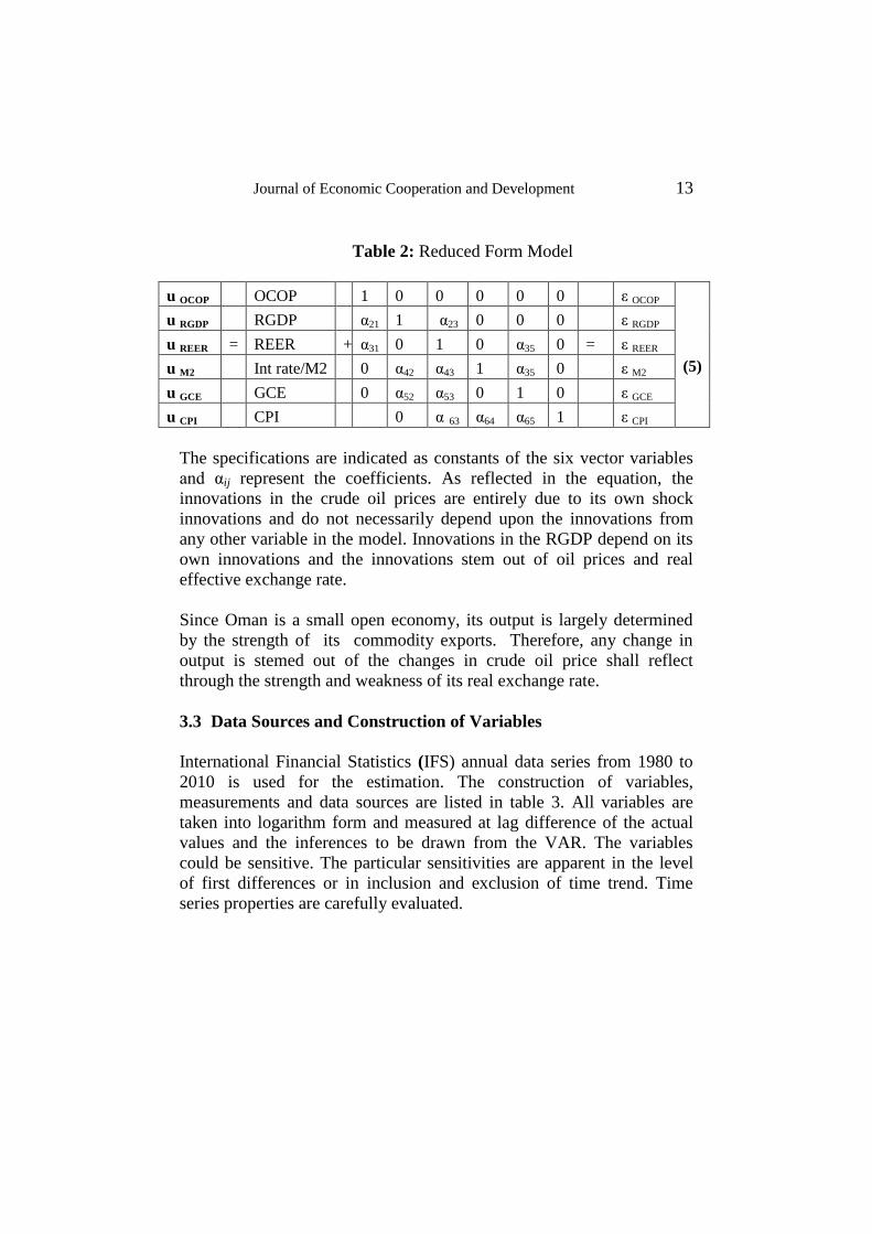
The identification scheme in equation 5 table 2 indicates specified
restrictions which are adopted in order to capture the joint behaviour of
interrelationship among the set of variables and their innovations.
Journal of Economic Cooperation and Development 13
Table 2: Reduced Form Model
u OCOP OCOP 1 0 0 0 0 0 ε OCOP
(5)
u RGDP RGDP α21 1 α23 0 0 0 ε RGDP
u REER = REER + α31 0 1 0 α35 0 = ε REER
u M2 Int rate/M2 0 α42 α43 1 α35 0 ε M2
u GCE GCE 0 α52 α53 0 1 0 ε GCE
u CPI CPI 0 α 63 α64 α65 1 ε CPI
The specifications are indicated as constants of the six vector variables
and αij represent the coefficients. As reflected in the equation, the
innovations in the crude oil prices are entirely due to its own shock
innovations and do not necessarily depend upon the innovations from
any other variable in the model. Innovations in the RGDP depend on its
own innovations and the innovations stem out of oil prices and real
effective exchange rate.
Since Oman is a small open economy, its output is largely determined
by the strength of its commodity exports. Therefore, any change in
output is stemed out of the changes in crude oil price shall reflect
through the strength and weakness of its real exchange rate.
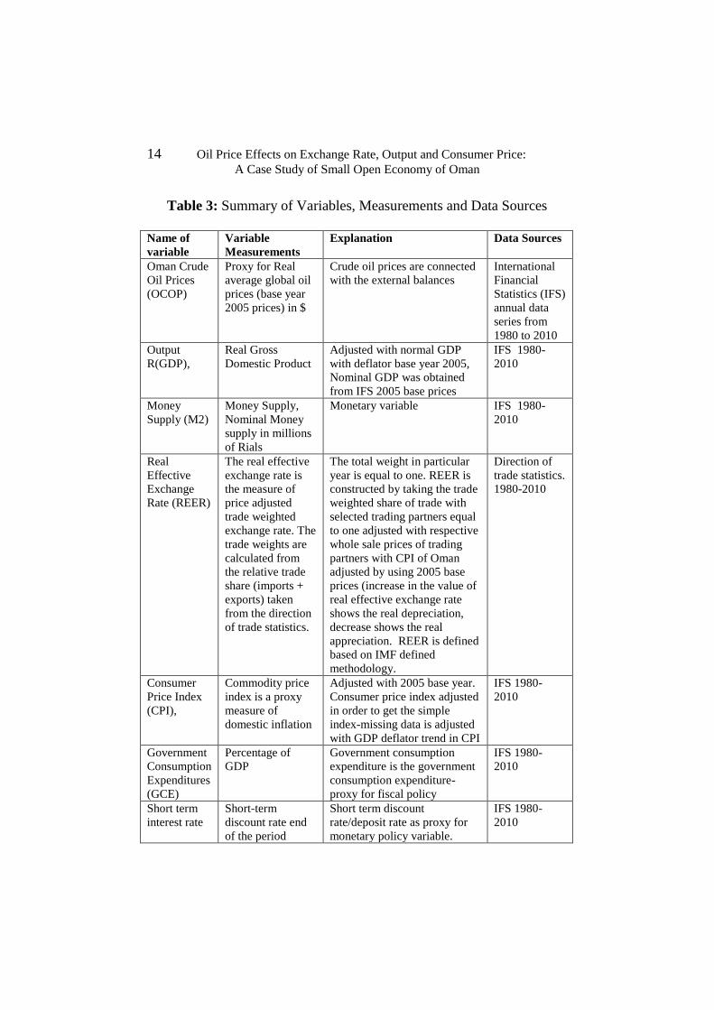
3.3 Data Sources and Construction of Variables
International Financial Statistics (IFS) annual data series from 1980 to
2010 is used for the estimation. The construction of variables,
measurements and data sources are listed in table 3. All variables are
taken into logarithm form and measured at lag difference of the actual
values and the inferences to be drawn from the VAR. The variables
could be sensitive. The particular sensitivities are apparent in the level
of first differences or in inclusion and exclusion of time trend. Time
series properties are carefully evaluated.
14 Oil Price Effects on Exchange Rate, Output and Consumer Price:
A Case Study of Small Open Economy of Oman
Table 3: Summary of Variables, Measurements and Data Sources
Name of
variable
Variable
Measurements
Explanation Data Sources
Oman Crude
Oil Prices
(OCOP)
Proxy for Real
average global oil
prices (base year
2005 prices) in $
Crude oil prices are connected
with the external balances
International
Financial
Statistics (IFS)
annual data
series from
1980 to 2010
Output
R(GDP),
Real Gross
Domestic Product
Adjusted with normal GDP
with deflator base year 2005,
Nominal GDP was obtained
from IFS 2005 base prices
IFS 1980-
2010
Money
Supply (M2)
Money Supply,
Nominal Money
supply in millions
of Rials
Monetary variable IFS 1980-
2010
Real
Effective
Exchange
Rate (REER)
The real effective
exchange rate is
the measure of
price adjusted
trade weighted
exchange rate. The
trade weights are
calculated from
the relative trade
share (imports +
exports) taken
from the direction
of trade statistics.
The total weight in particular
year is equal to one. REER is
constructed by taking the trade
weighted share of trade with
selected trading partners equal
to one adjusted with respective
whole sale prices of trading
partners with CPI of Oman
adjusted by using 2005 base
prices (increase in the value of
real effective exchange rate
shows the real depreciation,
decrease shows the real
appreciation. REER is defined
based on IMF defined
methodology.
Direction of
trade statistics.
1980-2010
Consumer
Price Index
(CPI),
Commodity price
index is a proxy
measure of
domestic inflation
Adjusted with 2005 base year.
Consumer price index adjusted
in order to get the simple
index-missing data is adjusted
with GDP deflator trend in CPI
IFS 1980-
2010
Government
Consumption
Expenditures
(GCE)
Percentage of
GDP
Government consumption
expenditure is the government
consumption expenditure-
proxy for fiscal policy
IFS 1980-
2010
Short term
interest rate
Short-term
discount rate end
of the period
Short term discount
rate/deposit rate as proxy for
monetary policy variable.
IFS 1980-
2010

Journal of Economic Cooperation and Development 15
4. Estimation and Result Discussion
Augmented Dickey Fuller (ADF) and Philips- Perron (PP) tests at level
and first difference are conducted. The first differencing variables are
integrated at different orders. Variables such as Real Gross Domestic
Product (RGDP), Government Consumption Expenditures (GCE) and
Consumer Price Index (CPI) variables are adjusted as rates of change
rather levels. Other variables such as Average Oman Crude Oil Price
(OCOP), Money Supply (M2) and Real Effective Exchange Rate
(REER) are used as level. Since the data series are in annual form, no
seasonal trend is observed and this has been verified and checked. Serial
correlation test is performed by using Lagrange Multiplier (LM)
statistics to check the robustness of ADF tests. Lag lengths are
determined by using Akaike Information Criterion (AIC).
The VAR model is estimated with log differences of six variables by
using yearly data with two lags in each equation. The two year lag
period is estimated over the period 1980-20107. Most of the variables
are found to be cointegarated. Therefore, the Vector Error Correction
model is used. The model allows the long term behaviour of the set of
endogenous variables to converge and cointegrating the long term
equilibrium relationship along with their short term dynamics. The
cointegration relationship is tested by using Johansen Cointegration Test
(1995). Four co-integrating vectors linking each other are found.
Cointegrating vectors are tested based on the trace and max-eigen
statistics. The cointegration relationship among the variables is
presented in the panel of table 4.
7 Charemza and Deadman (1992) suggest use of cointegrating vector for REER
variable, when it is used in long series, in short series, the variable may turns out to be
inconsistent in theoretical terms.

16 Oil Price Effects on Exchange Rate, Output and Consumer Price:
A Case Study of Small Open Economy of Oman
Table 4: Summary of the Reduced Form Estimation
The coefficient signs indicate the adjustments to the long run deviations.
Unlike the oil prices, the domestic prices are adjusted from a long run
path in a relatively longer time period than the adjustment in
goveronment expenditure which is relatively quick to adjust from its
deviations. The adjustment coefficient corresponds -0.04 per cent for
exchange rate, while for government consumption expenditure
coefficient is -0.288 and for real output, it is -0.171. Coefficients
suggest that government expenditure is relatively quick to adjust to the
equilibrium path, as compared to real output and real oil prices.
However, the real output responds to the external shocks relatively
slower than the response to government consumption expenditure. The
adjustment process indicates that output is positively responding to the
external shocks. Relatively slow adjustment in real oil prices and
domestic prices to equilibrium path indicate the long run relationship
among the two variables. Oman economy is a small economy, its
exportable share of commodities volume is very small compared to the
world demand. It seems less likely that oil prices of Oman crude affects
the global oil prices.
4.1 The Structural Model and Impulse Response Functions
The SVAR model suggested with structural restrictions in equation 5
and table 2 is estimated by using the VEC model. The results are
presented in the table 5. Structural response function of SVAR in a form
of coefficients in table 5 and Figure 3 indicates the generalized impulse
response functions.
Test statistics Average
Crude
Price of
Oil
RGDP Money
Supply
M2
REER Govt.
Cons Exp.
CPI
Co integration
equation
-0.04
(-0.34)
-0.171
(-2.45)
0.613
(2.66)
5.796
(3.30)
-0.288
(-2.34)
-0.005
(-0.06)
Goodness of fit statistics
Adjusted R2 0.46 0.21 0.52 0.51 0.64 0.18
SEE 0.02 0.00 0.08 4.77 0.02 0.01

Journal of Economic Cooperation and Development 17
Table 5: Structural VAR Regression Impulse Response Function of
SVAR ε OCOP = 0.05μ COP
(7.4)***
6.1
ε RGDP = 0.38 OCOP
(4.14)***
6.2
ε REER = 0.09 OCOP
(0.02)
4.50GCE 6.3
(0.47)
ε M2 = -2.67RGDP
(7.88)***
-0.02REER
(2.09)**
-0.25GCE 6.4
(2.1)**
ε GCE = +1.89RGDP
(3.85)***
-0.04REER
(1.51)
6.5
ε CPI = -1.34RGDP
(-3.13)***
-0.002REER
(0.88)
-0.32M2 6.6
(-2.4)***
The coefficients in table 5 are structural impulse response functions of
SVAR. These coefficients are driven from the vector error correction
and cointegrated series with structural restrictions. These coefficients
may not appear to be very precise. This may be possible because of the
estimation techniques and the nature of standard errors as cautioned by
(Bernanke, 1986; Calomiris and Hubbard, 1989, Turner, 199; Kiguel,
Lizondo and O’Connell, 1997).
4.2 Discussion
The results suggest that innovations in crude oil prices positively affect
the real output innovations (refer equation 6.1 in table 5). One
percentage point variation in real crude oil prices significantly impact
the real output by 0.38 per cent in the same direction. This means every
10 per cent increase in oil prices positively influence the real output by
3.8 per cent in long run. The innovations in real output also significantly
impact the changes in the money supply. However, these changes are
inconsistent with changes in real output growth. In the long run, shocks
in both real output and money supply become smooth. Changes in
output are primarily driven by changes in oil prices, whereas the
changes in output induce increase in money supply.

18 Oil Price Effects on Exchange Rate, Output and Consumer Price:
A Case Study of Small Open Economy of Oman
Figure 3: Response to Generalized One S.D Innovations to 2S.E
Journal of Economic Cooperation and Development 19
One percentage point increase in real Oman crude oil prices affects the
real exchange rate by 0.09 per cent, but this effect is statistically very
insignificant. This suggests that changes in global oil prices, in fact, do
affect the real exchange rate, but that effect is a very minor. Innovations
in real effective exchange rate affect the government consumption
expenditures positively but insignificantly. This result is consistent with
the trends in government consumption expenditures which are usually
increasing at the time of positive external balances. Innovations in real
exchange rates are having a negative and negligible impact on money
supply expansion. Changes in real output negatively affect the money
supply and it is quite clear that real output growth induces by the
external trade revenues but the output is not influenced by the changes
in domestic money supply. Innovations in real output infuence the
government consumption expenditures significantly and positively. One
percentage point increase in real output increases the government
consumption expenditure by 1.89 per cent. Innovations in output growth
affect the fiscal side of government consumption expenditure positively
and significantly. Real appreciation in exchange rate has a negligible
effect on prices. It means that real appreciation of exchange rate effect
on domestic prices is nominal. Because the domestic prices are not
much affected by appreciation or depreciation in real exchange rate. In
figure 3 response to generalized one standard deviation innovations to
two standard errors suggest consistency with the structural coefficients
in table 5. The results suggest negative response of external balances to
a real effective exchange rate. While real effective exchange rate has a
positive effect on real interest rate.
Pegged exchange rate policy seems to be performing well in anchoring
the inflationary expectation in Oman.. However, the changes in real
output significantly affect the prices negatively. Monetary expansion has
a negative effect on domestic prices. This also suggests that
expansionary monetary policy traces the pace of output and balances the
inflationary expectations. Oman has relatively stable prices in last few
decades. Every one per cent increases in money supply adjust the pace
of inflationary expectations by 0.32 per cent. Increase in output is
accompanied by decline in prices. This suggests that stabilization
policies works well with a mixture of expansion in output growth
coupled with monetary expansion accommodating the price changes.

20 Oil Price Effects on Exchange Rate, Output and Consumer Price:
A Case Study of Small Open Economy of Oman
The results are in line with the established theoretical propositions and
the evidence discussed earlier. The innovations in real effective
exchange rate not necessarily affect the consumer prices. However,
innovations to real output affect prices negatively. The relationship of
output innovations with government consumption expenditure positively
affect output which leads to an expansionary fiscal policy.
5. Conclusion
The study has examined the relationship of real oil prices shocks and its
channels to domestic macroeconomic dynamics of small open economy
of Oman. It has established the extent of interlinks of external and
domestic structural variants and their inter relationships. The dynamic
structural vector autoregressive econometric model along with stylized
structural variants of Oman economy has shed lights on the
interrelationship of macro variables and trace out their dynamic
moments. The results are consistent with the theory and provide the
important insights into the policy directions.
The results imply that crude oil price emerges to be a very significant
variable inducing output extends the monetary and government
consumption expenditures. In other words, changes in oil prices induce
output and consequent response to fiscal and monetary policy responses.
Monetary and fiscal policies anchor the global price shock and the long
run inflationary pressures. Monetary variables such as money supply
responses to changes in output and affects prices. The changes in
exchange rate are presumably positive shock to terms of trade or
external favourable effect. Results from impulse response functions
imply that innovation in output is influenced by oil prices. Exchange
rate, in fact, do appreciates due to increase in oil prices; the response to
fiscal expansion is derived out of changes in oil prices which is
straightforward theoretical result. Structural impulse response
coefficients indicate consistency with the earlier results.
Output and demand management policies in Oman economy are largely
dependent on the external factors, particularly oil prices. The shocks to
oil prices may likely affect the demand management policies. It seems in
the long run changes in oil prices determine the output and subsequent
fiscal and monetary policies which serve well to contain the inflationary

Journal of Economic Cooperation and Development 21
expectations and maintain positive external balances. In short run
fluctuations in oil prices or global imbalances though are contained well
in mixture of stabilization policies, continuation of a mixture of fiscal
and monetary stabilization policies may serve well the purpose of the
domestic dynamics of Oman economy. However, in the long run, over
reliance on stabilization policies in days of global imbalances may
provide fewer options to contain the external shocks. Therefore, the
exchange rate policy of pegging with dollar may be questionable in the
longer term.

22 Oil Price Effects on Exchange Rate, Output and Consumer Price:
A Case Study of Small Open Economy of Oman
References:
Abiad, A. G., Balakrishnan, R., Koeva Brooks, P., Leigh, D., & Tytell, I.
(2009), "What’s the damage? Medium-term output dynamics after
banking crises". IMF working papers, 1-37.
Agénor, P. R. (1991), "Output, devaluation and the real exchange rate in
developing countries". Weltwirtschaftliches Archiv, 127(1), 18-41.
Ahmed, S., & Loungani, P. (1999), Business cycles in emerging market
economies. Manuscript, IMF and Board of Governors of the Fed.
Aizenman, J., & Riera-Crichton, D. (2008), "Real exchange rate and
international reserves in an era of growing financial and trade
integration," The Review of Economics and Statistics, 90(4), 812-815.
Allsopp, C. (2006), "Why is the Macroeconomic Impact of Oil Prices
Different this Time?," In Oxford Energy Forum (Vol. 66, p. 20). The
Oxford Institute for Energy Studies.
Amano, R. A., & Van Norden, S. (1995), "Terms of trade and real
exchange rates: the Canadian evidence" Journal of International Money
and Finance, 14(1), 83-104.
Bayoumi, T., & Symansky, S (1994), The Robustness of Equilibrium
Exchange Rate Calculations to Alternative Assumptions and
Methodologies, (eds) John Williamson, equilibrium exchange rates.
Peterson Institute, 1994,pp. 19–59.
Bahmani-Oskooee, M., & Kutan, A. M. (2008), "Are devaluations
contractionary in emerging economies of Eastern Europe?". Economic
Change and Restructuring, 41(1), 61-74.
Carvalho Filho, I. E., & Bems, R. (2009), "Exchange rate assessments:
methodologies for oil exporting countries", IMF Working Papers, 1-35.
Bhattacharya, R. (2003), "Sources of variation in regional economies,"
The Annals of Regional science, 37(2), 291-302.

Journal of Economic Cooperation and Development 23
Blanchard, O. J., & Watson, M. W. (1986), "Are business cycles all
alike?," In The American business cycle: Continuity and change (pp.
123-180). University of Chicago Press.
Bernanke, B. S. (1986), "Alternative explanations of the money-income
correlation" In Carnegie-Rochester conference series on public policy
(Vol. 25, pp. 49-99). North-Holland.
Calvo, G. A., Reinhart, C. M., & Vegh, C. A. (1995), "Targeting the real
exchange rate: theory and evidence," Journal of Development
Economics, 47(1), 97-133.
Canetti, E. (1991), Monetary growth and exchange rate depreciation as
causes of inflation in African countries: An empirical analysis. (eds)
Centre for Economic Research on Africa Research Monograph Series,
School of Business-Montclair State University, New Jersey.
Cashin, P., Céspedes, L. F., & Sahay, R. (2004), "Commodity currencies
and the real exchange rate," Journal of Development Economics, 75(1),
239-268.
Clarida, Richard., Gali, Jordi., Gertler, Mark (1999), "The Science of
Monetary Policy: A New Keynesian Perspective," Journal of Economic
Literature, 37/ 2 : 1661-1707.
Calomiris, C. W., & Hubbard, R. G. (1989), "Price flexibility, credit
availability, and economic fluctuations: evidence from the United States,
1894-1909," The Quarterly Journal of Economics, 429-452.
Central Bank of Oman (2014), Annual Report 2014, Sultanate of Oman
Charemza, W.W. and Deadman, D.F. (1992), New Directions in
Econometric Practice, Edward Elgar: Aldershot
Chen, Yu-chin. Kenneth, Rogoff. (2003), “Commodity currencies,”
Journal of International Economics, 60/1: 133-160.

24 Oil Price Effects on Exchange Rate, Output and Consumer Price:
A Case Study of Small Open Economy of Oman
Copelman, M., & Werner, A. M. (1995), "The monetary transmission
mechanism in Mexico" (No. 521). Board of Governors of the Federal
Reserve System.
Coudert, V., Couharde, C., & Mignon, V. (2008), "Do terms of trade
drive real exchange rates? Comparing oil and commodity currencies,"
Centre d'Etudes Prospectives et d'Informations Internationales (CEPII),
Paris, 32.
Dornbusch, R., Sturzenegger, F., Wolf, H., Fischer, S., & Barro, R. J.
(1990), "Extreme inflation: dynamics and stabilization," Brookings
Papers on Economic Activity, 1990(2), 1-84.
Edwards, S. (1989), Real Exchange Rates, Devaluation, and
Adjustment: Exchange Rate Policy in Developing Countries,
Cambridge, Mass.: MIT Press
Elbadawi, I. A. (1990), "Inflationary process, stabilization and the role
of public expenditure in Uganda," Washington, DC: World Bank.
Gala, P., & Lucinda, C. R. (2006), "Exchange rate misalignment and
growth: old and new econometric evidence," Revista Economia, 7(4),
165-187.
Ghosh, A. R., Gulde, A. M., Ostry, J. D., & Wolf, H. C. (1997), "Does
the nominal exchange rate regime matter?" (No. w5874). National
Bureau of Economic Research.
Habib, M. M., & Kalamova, M. M. (2007), "Are there oil currencies?
The real exchange rate of oil exporting countries," Working Paper, No.
839, European Central Bank.
Hakro, A. N., & Omezzine, A. M. (2010), "Macroeconomic effects of
oil and food price shocks to the oman economy," Middle Eastern
Finance and Economics, 6(2010), 72-89.
Hirata, H., Kim, S. H., & Kose, M. A. (2004), "Integration and
fluctuations: the case of MENA," Emerging Markets Finance and
Trade, 40(6), 48-67.

Journal of Economic Cooperation and Development 25
Hoffmaister, A. W., & Roldós, J. E. (1997), "Are business cycles
different in Asia and Latin America?"Working Paper No. 97/9,
International Monetary Fund.
Hoffmaister, A. W., & Végh, C. A. (1996), "Disinflation and the
recession-now-versus-recession-later hypothesis: evidence from
Uruguay," Staff Papers-International Monetary Fund, 355-394.
Hahn, E. (2003), "Pass-through of external shocks to euro area
inflation," Working paper, 243, European Central Bank.
Isard, P., & Faruqee, H. (1998), "Exchange rate assessment: extension of
the macroeconomic balance approach" (Vol. 167). International
monetary fund.
Ito, T., & Sato, K. (2006), "Exchange rate changes and inflation in post-
crisis Asian economies: VAR analysis of the exchange rate pass-
through" (No. w12395). National Bureau of Economic Research.
Jbili, A., & Kramarenko, V. (2003), "Choosing exchange regimes in the
Middle East and North Africa," International Monetary Fund
Kamin, S. B., & Klau, M. (1998), "Some multi-country evidence on the
effects of real exchange rates on output," FRB International Finance
Discussion Paper, (611).
Kamin, S. B. (1996), "Real Exchange rates and Inflation in exchange-
Rate based Stabilizations: an empirical examination," International
Finance Discussion Papers, (554).
Kamin, S. B., & Rogers, J. H. (2000), "Output and the real exchange
rate in developing countries: an application to Mexico," Journal of
development economics, 61(1), 85-109.
Kiguel, M. A., Lizondo, J. S., & O'Connell, S. A. (Eds.). (1997),
Parallel Exchange Rates in Developing Countries. St. Martin's Press.

26 Oil Price Effects on Exchange Rate, Output and Consumer Price:
A Case Study of Small Open Economy of Oman
Kim, S. H., & Ahn, H. D. (2005), "Dynamics of open economy business
cycle models: the case of Korea," Korea Development Review, 1(1),
157-84.
Korhonen, I. and T. Juurikkala (2007), "Equilibrium exchange rates in
oil-dependent countries," BOFIT Discussion Papers No. 8.
Kose, M. A. (2002), "Explaining business cycles in small open
economies:‘How much do world prices matter?," Journal of
International Economics, 56(2), 299-327.
London, A. (1989), "Money, inflation and adjustment policy in Africa:
some further evidence," African Development Review, 1(1), 87-111.
MacDonald, R., & Ricci, L. A. (2001). "PPP and the Balassa Samuelson
effect: The role of the distribution sector," (Vol. 442). International
Monetary Fund.
Makdisi, S., Fattah, Z., & Limam, I. (2006), "Determinants of Growth in
the MENA Countries," Contributions to economic analysis, 278, 31-60.
McCarthy, J. (2000), "Pass-through of exchange rates and import prices
to domestic inflation in some industrialized economies," FRB of New
York Staff Report, (111).
Mendoza, E. G. (1995), "The terms of trade, the real exchange rate, and
economic fluctuations," International Economic Review, 101-137.
Montiel, P. J. (1989), "Empirical analysis of high-inflation episodes in
Argentina, Brazil, and Israel," Staff Papers-International Monetary
Fund, 527-549.
Morley, S. A. (1995),. "Structural adjustment and the determinants of
poverty in Latin America," Coping with austerity: Poverty and
inequality in Latin America, 42.
Ndung’u, Njuguna. (1993), Dynamics of the Inflationary Process in
Kenya, Göteborg: University of Göteborg.

Journal of Economic Cooperation and Development 27
Ndung'u, N. S. (1997), "Price and Exchange Rate Dynamics in Kenya:
An Empirical Investigation," (No. 58).African Economic Resarch
Consortium (AERC)African Economic Research Consortium, AERC
Research Paper /58.
Odusola, A. F., & Akinlo, A. E. (2001),"Output, inflation, and exchange
rate in developing countries: An application to Nigeria," The Developing
Economies, 39(2), 199-222.
Odedokun, M. O. (1997)," Dynamics of inflation in Sub-Saharan Africa:
the role of foreign inflation, official and parallel market exchange rates,
and monetary growth," Applied Financial Economics, 7(4), 395-402.
Ricci, M. L. A., Lee, M. J., & Milesi-Ferretti, M. G. M. (2008), "Real
exchange rates and fundamentals: A cross-country perspective," (No. 8-
13). International Monetary Fund.
Rodriguez, G. H., & Gazani, G. D. (1995), "Fluctuaciones
macroeconómicas en la economía peruana" Banco Central de la
República Dominicana.
Rodrik, D. (2008), "Normalizing industrial policy," International Bank
for Reconstruction and Development/The World Bank.
Rogers, J. H., & Wang, P. (1995), "Output, inflation, and stabilization in
a small open economy: evidence from Mexico," journal of Development
Economics, 46(2), 271-293.
Roubini, Nouriel, and Brad Setser. (2004), "The US as a net debtor: The
sustainabil- ity of the U.S. external imbalances," New York University.
Mimeograph.
Santaella, J. A., & Vela, A. (1996),"The 1987 Mexican disinflation
program: an exchange rate-based stabilization?" International Monetary
Fund.

28 Oil Price Effects on Exchange Rate, Output and Consumer Price:
A Case Study of Small Open Economy of Oman
Schneider, M., & Tornell, A. (2004), "Balance sheet effects, bailout
guarantees and financial crises," The Review of Economic Studies, 71(3),
883-913.
Setser, B. (2007), "The case for exchange rate flexibility in oil-exporting
economies," (No. PB07-8). Peterson Institute for International
Economics.
Shahin, Wassim and Elias El-Achkar,( 2010), "Regional Monetary
Coordination between GCC Monetary Union and Other MENA
Countries," paper presented at the workshop, "The Evolving
International Role of the GCC," Economies at the Mediterranean
Research Meeting of the European University Institute.
Times of Oman, (2008), Daily Times of Oman, Muscat, 16 March,
Muscat, Sultanate of Oman.
Turner, P. M. (1993),. "A structural vector autoregression model of the
UK business cycle," Scottish Journal of Political Economy, 40(2), 143-
164.
Vinh, Nguyen Thi Thuy, and Seiichi Fujita (2001), "The impact of real
exchange rate on output and inflation in Vietnam: A VAR approach,"
Pesaran, M., Y.Shin and R. Smith (2001). "Bounds testing approaches to
the analysis of level relationships", Journal of Applied Econometrics 16
(2007): 289-326.
Williamson, J. (1994), Estimating equilibrium exchange rates. Peterson
Institute.

Journal of Economic Cooperation and Development, 37, 3 (2016), 29-56
The Impacts of Foreign Labour Entry on the Labour Productivity
in the Malaysian Manufacturing Sector
Nur Sabrina Mohd Palel
1, Rahmah Ismail
2 and Abdul Hair Awang
3
Improvement and strengthening of labour productivity is an important
approach to accelerate the growth of the manufacturing sector in Malaysia.
This study attempts to analyses the impacts of the entry of foreign workers on
the labour productivity of the manufacturing sector in Malaysia. The analysis
of this study employs the dynamic panel data method which combines time
series and cross-section data. The data used was from the year 1990 to 2008,
covering 15 selected sub-sectors in the Malaysia manufacturing sector. Core to
the analysis in the study is the Pooled Mean Group (PMG) estimation model.
The study found that foreign labour, local labour, capital intensity and foreign
direct investment (FDI) have positive and significant effects on the labour
productivity growth. The study differentiates between local and foreign labour
into categories of skilled and unskilled labour. The findings indicated that
unskilled foreign and local labour are negatively and significantly affect the
growth of labour productivity in the long run. Inversely, skilled local and
foreign labour had a significant and positive impact on the labour productivity
growth. However, the contribution of foreign labour on labour productivity is
smaller compared to the local labour.
1. Introduction
Labour productivity is an important, frequently emphasised element in
any sector as part of an effort to keep a sector competitive in the global
market. The growth of the industrial sector has been successful in
increasing export and this effectively led to the innovation of new
1 MEc Student, Faculty of Economics and Management, Universiti Kebangsaan
Malaysia Email:nur02862yahoo.com 2 Senior Lecturer, Faculty of Economics and Management, Universiti Kebangsaan
Malaysia Email:[email protected] 3 Senior Lecturer, Faculty of Social Sciences and Humanities,Universiti Kebangsaan
Malaysia Email: [email protected]

30 The Impacts of Foreign Labour Entry on the Labour Productivity
in the Malaysian Manufacturing Sector
technologies and improvements in the internal management of firms.
Since independence, Malaysia has experienced encouraging phases of
economic development through various economic development policies
and strategies. In fact, before the Asian financial crisis in the year 1997,
the country is known as one of the rapidly growing economies on par
with the developed economies in East Asia such as Japan, South Korea,
Taiwan and Hong Kong (Ishak Yussof & Nor Aini, 2009). A rapidly
growing manufacturing sector can speed up the growth of an economy
due to its share in the Gross Domestic Product (GDP), job creation and
foreign exchange. One of the most effective ways to further improve this
sector is by improving labour productivity. The logic is simple; a higher
productivity means that the same number of inputs can produce higher
quantities of output. Sahar (2002) explains that a high labour
productivity in the manufacturing sector can help create sustainable
growth and development of a country.
Economic growth is an important determinant of national development
and these are two interrelated concepts. A country can grow without
developing, but to develop, a country needs to grow. Economic growth
requires a combination of a number of factors, including labour, land,
capital and technology being employed efficiently without waste.
Labour - local and foreign - is an important part of this equation. In
general, the rationale behind employing foreign labour is to fill the gap
create by the shortage of labour supply in the local labour market
especially in sectors like farming, construction, service, industrial and
manufacturing. This is a short term solution according to Preibisch
(2007). Nevertheless, the output generated through the foreign labour
contributes positively to the country's export.
It must be noted that foreign labour has contributed to Malaysia's
economic growth, especially with regard to the GDP and aggregate
expenditure. The government has effectively prevented excessive
increases in wages and inflation. The wages paid to the foreign workers
are considerably lower than the what the locals receive. Despite the
relatively lower wages, the foreign labour positively contribute to
increase in demand (Borjas, 2006). However, being a short-term
solution, the economy cannot continuously depend on the contributions
of foreign workers. With the country looking to become a high earning
economy by 2020, a switch of strategy is important and thus, rather than

Journal of Economic Cooperation and Development 31
relying on the number of inputs, more emphasis should be given to
increasing productivity of input.
An influx of foreign workers can affect an economy both positively and
negatively. Its influence on the labour market depends on its role,
whether as a substitute or a complement to the local workers. Borjas
(1993) found a negative impact of foreign workers. However, he
stressed that such negative influence is only valid for unskilled foreign
labour. The direction of the effects of foreign worker entry on a market
depends on their productivity. Highly productive, skilled foreign worker
can immensely contribute to an (Hercowitz et al. 1999). On the other
hand, unskilled foreign workers may have problems adapting and may
end up needing more help than contributing. It is worth noting that
several studies have been conducted on this topic but the results have
been inconsistent. As such, the issue is very much inconclusive. It is
therefore imperative for researchers to keep on studying the subject and
more importantly on the factors that make the results so inconsistent.
Compared to more developed economies like China, Singapore and
South Korea, our labour productivity is still relatively modest (Malaysia
Productivity Corporation, 2013). A shortage of labour during the period
of the 7th Malaysia Plan (7MP) has tightened the labour market and
pushed wages up. As part of the effort to reduce the shortage, a
programme was initiated to allow for foreign workers entry. It was,
however, at that time, unclear how the influx of skilled and unskilled
foreign workers can generate growth of the manufacturing sector in the
longer term.
Overall, the study aims to contribute to the literature on this topic
through its measurement method which was used to estimate the impact
of foreign workers entry on labour productivity. The method is known
as Autoregressive Distributed Lag (ARDL) dynamic panel test method
using Pooled Mean Group (PMG) estimation model. This method
allows the researcher to observe the relationship between the
independent and dependent variables in the short and long terms.
Furthermore, this study provides a more detailed insight by dividing the
foreign labour into skilled and unskilled categories.
The objective of this study is to analyse the short and long term effects
of foreign worker entry in general on the productivity of labour. The

32 The Impacts of Foreign Labour Entry on the Labour Productivity
in the Malaysian Manufacturing Sector
study also sought to examine the influences of the use of foreign and
local, skilled and unskilled labour on the productivity of labour. This
paper is organised into five sections, namely introduction, literature
review, methodologies, research findings and the last part from this
study is conclusions and suggestions.
1.1 Trend of Foreign Labour in Malaysia
Rapid economic development has led to rapid changes in the labour
market. With demand for labour increasing more than the supply, there
was a need to address this shortage by allowing entry of foreign workers
into the domestic market. As a result, there has been a steady influx of
foreign workers from various countries such as Indonesia, India, Nepal,
Bangladesh and Filipina. Table 1 summarises the development of the
entry of foreign workers into Malaysia from the year 2007 to 2011. It is
clear, however, that while entry is still occurring, the numbers were
declining steadily. Manufacturing sector recorded the highest inflow of
foreign workers from year 2007 to year 2011 compared to other sectors.
Local Electrical and Electronics (E &E) industry was the main sector
contributing 55.9 percent of the country's exports and employs 28.8
percent of the national labour force (Prime Minister's Department,
2012). This industry has also successfully developed the ability and
skills for the manufacturing sector, consumer electronics, and electronic
and electrical components. Productivity generated by foreign labour has
helped increase total exports and consequently contribute to the surplus
in the balance of payments. Strong export revenue growth is directly
driven by high export value. Therefore, the enhancement and
strengthening of productivity is one approach that can be taken to
accelerate the growth of the manufacturing sector in Malaysia.

Journal of Economic Cooperation and Development 33
Table 1:Number of foreign labour in Malaysia by sector , 2007-2011 (’000).
Sector 2007 2008 2009 2010 2011
Total 2,044,805 2,062,596 1,918,146 1,817,871 1,5730,61
Agriculture 165,698
(8.1)
186,967
(9)
181,660
(9.4)
231,515
(12.7)
152,325
(9.6)
Farming 337,503
(16.5)
333,900
(16.1)
318,250
(16.5)
266,196
(14.6)
299,217
(19)
Manufacturing 733,372
(35.8)
728,867
(35.3)
663,667
(34.5)
672,823
(37)
580,820
(36.9)
Construction 293,509
(14.3)
306,873
(14.8)
299,575
(15.6)
235,010
(12.9)
223,688
(14.2)
Service 200,428
(9.8)
212,630
(10.3)
203,639
(10.6)
165,258
(9)
132,919
(8.4)
House maid 314,295
(15.3)
293,359
(14.2)
251 355
(13.1)
247,069
(13.5)
184,092
(11.7)
Source: Ministry of Home Affairs, various years.
Note: Values in bracket are percentage.
In the duration of the 9MP, the government was committed to reform the
labour market, with particular emphasis on the increased mobility of
labour and increasing the skills of the workforce. Labour market reforms
were essential to provide a platform for the country to continue to grow
towards becoming a high income economy.
Table 2: Number of foreign labour by skill (’000) for the year 1990-2008
Source: Department of Statistics Malaysia, various years.
Table 2 reports that the number of unskilled foreign workers has more
than doubled in the 2000s compared to the 1990s (from 86,847 in 1990
to 198,876 in 2000). This influx of unskilled foreign workers can be
attributed to the unwillingness of the locals to be involved in
occupations which has the features of 3D (Dirty, Dangerous, Difficult).
Year Skilled Unskilled
1990 9,154 86,847
1995 7,016 104,665
2000 6,986 198,876
2005 9,022 336,055
2008 11,245 421,985
34 The Impacts of Foreign Labour Entry on the Labour Productivity
in the Malaysian Manufacturing Sector
Meanwhile, the number of skilled foreign labour has shown a steady
decrease from the year 1990 until 2000 but steadily increased again until
2008. The skilled foreign workers are complements to the local skilled
workers and a combination of both is needed to facilitate the growth of
the economy towards becoming more competitive.
2. Literature Review
Productivity refers to the comparison between the output and the input
used to produce it. The inputs for a business are resources within an
organisation which include human capital, finances, etc. while output is
the product produced using the available input (Braid 1983; Prokopenko
1987). Most of the definitions of productivity are related to the
measurement of efficiency of input in the production of output and the
measurement of effectiveness by observing the ratio between the actual
output and the projected output (Pritchard, 1995).
Peri (2012) used the Cobb Douglas function to examine the long-term
effects of the entry of foreign workers on the American labour market
for the year 1960, 2000 and 2006. The findings indicate that foreign
workers have a positive effect on the specialisation of local workers.
Moreover, no evidence that foreign labour crowded-out employment,
rather it encourages efficient specialisation and encourages better use of
technology among the less skilled workers.
Huber et al. (2010), on the contrary, explains the entry of foreign
workers in a more negative light. They explained that locals normally
view foreigners as a threat to their employability. With increasing
population and labour supply, such view is natural. They also studied on
the roles of skilled foreign workers and how qualified they are for their
jobs. They noted a positive contribution from the foreign workers on
labour productivity in skill-intensive industries.
According to Zaleha et al (2011), the increasing entry of foreign workers
into Malaysia is related to its strong economic growth. The Cobb
Douglas production function was used as the basic to form their labour
productivity model with the data ranging from the year 1972 to the year
2005. Their findings indicate that foreign workers contribute positively
to the productivity of labour in this country with improvements of 0.172
percent in labour productivity with a 1 percent increase in foreign

Journal of Economic Cooperation and Development 35
labour. However, their findings also showed a negative effect between
labour productivity and capital labour ratio. This shows that the
Malaysian manufacturing sector is still labour intensive in nature, since
any increase in capital usage,will leads to increase in capital labour ratio
and this negatively affects labour productivity.
Llull (2008), meanwhile, is of the opinion that an immigration of
workers into a country adversely affect the country's productivity. The
argument is that the entry of foreign worker into a firm lowers its
average wage. The estimation took into account the effects of inverse
causality. The researcher also analysed the impact of foreign labour on a
country's per capita GDP. The findings showed a negative and
insignificant impact on productivity. On the contrary, Chia (2011)
argues that foreign workers can increase a country's GDP and
simultaneously fill the needs for workers in Singapore. However, the
study also mentioned that dependence on foreign workers can slow
down economic restructuring and ultimately affect national productivity
adversely. At the end of the study, the researcher advised the
Singaporean government to reduce its dependency on foreign workers to
improve its productivity.
FDI is an important role in the development process in many countries.
FDI generally provides capital and technology to developing countries.
Hale and Long (2006) found that there were positive effects on labour
productivity as a result of the spill-over effects of FDI. They used a
survey of 1,500 firms in China to determine whether there are
technology spill-overs from foreign firms to domestic firms in the same
city and the same industry. The same outcome was found from the study
by Salim and Bloch (2009), found that FDI is an important contributor
to the growth of the chemical industry in Indonesia.Tanna (2009)
studied the relations between FDI and the changes in productivity of
banks. Using data between the years 2000 and 2004 which was obtained
through observation method covering 566 commercial banks, the
analysis was conducted in two stages - firstly, a non-parametric
Malmquist method was used to explain the changes in TFP for bank's
efficiencies of scale, and secondly to explain the changes in technology.
An analysis was also conducted to examine the influences of FDI on
productivity. The study found that FDI has a negative effect in the short
term, but affect productivity positively in the long term. This finding is
consistent with the Malmquist analysis.

36 The Impacts of Foreign Labour Entry on the Labour Productivity
in the Malaysian Manufacturing Sector
Meanwhile, Mohammad Sharif Karimi and Zulkormain (2009) examine
the relationship between FDI and productivity growth using the Todo-
Yamamoto test to understand the causality relation and bounds testing
(ARDL). They used data between 1970 and 2005 in Malaysia. They
found that there is no strong evidence for bi-directional causality and
long-term relationship between FDI and productivity growth.
Thangavelu and Owyong (2003) studied the relationship between export
performance and productivity growth in the Singapore manufacturing
sector. A panel data of 10 major industries in the manufacturing sector
were analysed for the duration between 1974 and 1995. The findings
suggest that growth in labour productivity helps improve export growth
for sub-sectors of selected industries. They also found that FDI-intensive
industries contribute more to labour productivity in the manufacturing
sector than industries which are not FDI-intensive.
Rahmah et al (2012) states that globalisation and technological
advancement increase the demand for high-quality labour. The
researcher examined the impact of globalisation on labour productivity
in the manufacturing sector in Malaysia. This study examined 5 sub-
industries, namely production, processing and preservation of meat,
fisheries, fruits, vegetables, oil and fat (151), manufacturing of refined
petroleum products (232), basic chemical manufacturing (241), iron and
steel manufacturing, office machinery manufacturing, accounting and
computing machinery (300) as well as the manufacturing of electric
valves and tubes and other electronic components, component (321).
Data used include duration of time from the year 1985 to 2007. This
study uses the data panel method choosing between fixed effects to
examine the relationship between labour productivity and capital labour
ratio, export import ratio, FDI, technology transfer and foreign labour.
The study found that globalisation indicators such as FDI and openness
of an economy has a negative and significant effect on labour
productivity. Meanwhile, capital labour ratio significantly influences
labour productivity growth in the manufacturing sector in general as
well as its sub-sectors.
3. Methodology
The analysis in this study uses dynamic panel data methods that
combine time series data (t) and cross-sectional data (n) with t larger
than n. n is the 15 sub-sectors in the manufacturing sector based on 5-
Journal of Economic Cooperation and Development 37
digit Standard Industrial Classification Malaysia (MSIC), while t is 19
years from the year 1990 until 2008. The data used in this study are a
secondary data obtained from the Manufacturing Industry Survey
conducted by the Department of Statistics (DOS). Other data used were
obtained from the Ministry of International Trade and Industry (MITI)
and Malaysian Industrial Development Authority (MIDA). The data was
analysed using the software Stata 10.1. The approach used in the
analysis was Pooled Mean Group (PMG) regression. The study also
employed the Hausman Test to help value the statistical model between
the Mean Group (MG) and PMG to choose the more suitable model for
the available data. To test the stationary of data, the unit root test was
conducted based on the standards of Augmented Dickey Fuller (ADF)
and Philips Perron (PP). Labour productivity is derived from the total
output divided by total labour. Next, the productivity obtained was
assigned as the dependent variable while independent variables are
composed of capital intensity, FDI and labour types of foreign and
domestic labour. For each category of labour, they will be split into two
groups - skilled and unskilled workers.
The dependent variable in this study is labour productivity. In this study,
the output value (production) of 15 sub-sectors of manufacturing is used,
with real production value deduced with Producer Price Index (PPI) year
2000=100 as the base year. The independent variable used is capital
intensity (KL) which is the total fixed asset owned by firms in January
divided by the number of labour involved in the manufacturing sub-
sector, FDI, total number of foreign labour and local labour. The skill
category variable is divided into skilled and unskilled labour. Skills refer
to their abilities and education levels.
3.1 Model Specification
Productivity can be defined as the value or the quantity of output that
can be generated by all units of input. Outputs are products or service
produced by the organisation. In other words, productivity is a concept
that describes the relationship between the output produced by an
organization with the inputs used. In a nutshell, it measures the
efficiency and effectiveness of each unit of input.
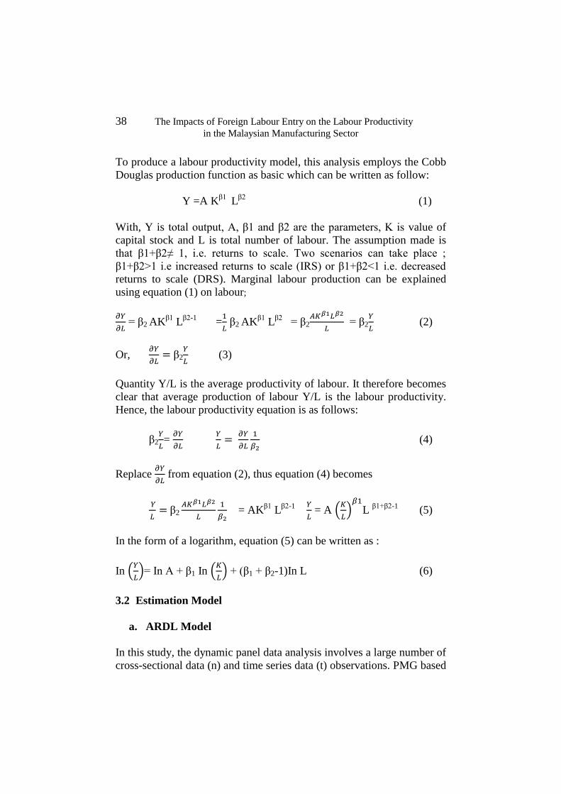
38 The Impacts of Foreign Labour Entry on the Labour Productivity
in the Malaysian Manufacturing Sector
To produce a labour productivity model, this analysis employs the Cobb
Douglas production function as basic which can be written as follow:
Y =A Kβ1
Lβ2
(1)
With, Y is total output, A, β1 and β2 are the parameters, K is value of
capital stock and L is total number of labour. The assumption made is
that β1+β2≠ 1, i.e. returns to scale. Two scenarios can take place ;
β1+β2>1 i.e increased returns to scale (IRS) or β1+β2<1 i.e. decreased
returns to scale (DRS). Marginal labour production can be explained
using equation (1) on labour;
𝜕𝑌
𝜕𝐿 = β2 AK
β1 L
β2-1 =
1
𝐿 β2 AK
β1 L
β2 = β2
𝐴𝐾𝛽1𝐿𝛽2
𝐿 = β2
𝑌
𝐿 (2)
Or, 𝜕𝑌
𝜕𝐿= β2
𝑌
𝐿 (3)
Quantity Y/L is the average productivity of labour. It therefore becomes
clear that average production of labour Y/L is the labour productivity.
Hence, the labour productivity equation is as follows:
β2𝑌
𝐿=
𝜕𝑌
𝜕𝐿
𝑌
𝐿=
𝜕𝑌
𝜕𝐿
1
𝛽2 (4)
Replace 𝜕𝑌
𝜕𝐿 from equation (2), thus equation (4) becomes
𝑌
𝐿= β2
𝐴𝐾𝛽1𝐿𝛽2
𝐿
1
𝛽2 = AK
β1 L
β2-1 𝑌
𝐿 = A (
𝐾
𝐿)
𝛽1
L β1+β2-1
(5)
In the form of a logarithm, equation (5) can be written as :
In (𝑌
𝐿)= In A + β1 In (
𝐾
𝐿) + (β1 + β2-1)In L (6)
3.2 Estimation Model
a. ARDL Model
In this study, the dynamic panel data analysis involves a large number of
cross-sectional data (n) and time series data (t) observations. PMG based

Journal of Economic Cooperation and Development 39
on Autoregressive Distributed Lag (ARDL) panel model can determine
the short-term and long-term relationship of a model. By using this
estimation, the intersection, the slope coefficient and standard deviation
are allowed to differentiate the entire group. Assume ARDL (p,
q1,…..qk), the dynamic panel equation can be written as below: -
(7)
With yit as the dependent variable i.e. productivity (Y/L), Xit as vektor k
x 1 as the qualifier variable, µi representing effects of specific groups
(fixed effects), 𝜙𝑖 as the multiplier for dependent variable lag, βi as the
multiplier vector k x 1 qualifier variable, λ*i j multiplier for dependent
variable at lagged first-differences and yi,j is the vector multiplier k x 1
for qualifier variable at lagged first-differences and the value lagged and
i is the manufacturing sub-sector and t is the year.
The main assumption of the ARDL model is that 𝑢𝑖𝑗 is independently
distributed with mean value equals to 0 and standadrd deviation 𝛿2> 0.
It further assumes that error correction term (ec) 𝜙𝑖< 0 for all i ,
meaning that there exist a long-term relationship between 𝑦𝑖𝑡and 𝑥𝑖𝑡.
The long-term relationship can also be written as follows:
𝑦𝑖𝑡 = 𝜃′𝑖𝑗𝑥𝑖𝑗 + Ƞ𝑖𝑗𝑖 = 1,2, … . . 𝑁; 𝑡 = 1,2, … … 𝑇 (8)
With 𝜃′𝑖𝑗 = −𝛽𝑡′
𝜙𝑖 being the multiplier vector k x 1 which is the long-
term coeeficient and Ƞ𝑖𝑗 is stationary with the probability of non-zero
mean which involves fixed effects. Equation (7) can be re-written in the
VECM (Vector Error Correction Model ) system as follows:
∆𝑦𝑖𝑡 = 𝜙𝑖Ƞ𝑖,𝑡−1 + ∑ 𝜆𝑖𝑗
𝑝−1
𝑗=1
∆𝑦𝑖,𝑡−𝑗 + ∑ 𝛿′𝑖,𝑗
𝑞−1
𝑗=0
∆𝑥𝑖,𝑡−𝑗 + µ𝑖
+ µ𝑖𝑡 (9)
With Ƞ𝑖,𝑡−1 as the error variable generated from the long term equation
in (8), 𝜙𝑖 as the error correction term to adjust the balance in the long
term. If 𝜙𝑖 =0, then there is no long term relationship between the
dependent and independent variables. The parameter must be expected
1
1
1
0
,
'
,
*
1,
'
1,
p
j
q
j
itijtiijjtiijtiitiiit uxyxyy

40 The Impacts of Foreign Labour Entry on the Labour Productivity
in the Malaysian Manufacturing Sector
to be significantly negative under the main assumption which shows that
the variables returns to balance in the long term.
Intervals order in the ARDL model is determined using either the
information criteria of Akaike (AIC) or Schwartz Bayesian (SBC)
before the chosen model is estimated using the ordinary least squares
method. Although the estimated value obtained is the same, the standard
deviation estimation of the model chosen by AIC is smaller. However,
the interval order chosen by AIC is higher that the one chosen by SBC.
b. Estimation Model
To identify the short-term and long-term relationships between foreign
labour entry on labour productivity, the model below was estimated:-
Model 1
(10)
Model 2
(11)
1,
31,21,1
1,1
0 '''ln
ti
titi
tii
it L
KInInFwInLw
L
Y
L
YIn
jtij
p
j
q
j
q
j
jtij
jti
jti InFwInLwL
YInFDI
,,21
1
1
1
0
1
0
,,11
,
11,4 **ln'
tjti
q
j
j
jti
q
j
j InFDIL
KIn 1,
1
0
,41
,
1
0
,31 **
1,31,21,
'
1
1,2
0 ''ln
tititi
tii
it
InskillFwwInunskillLInskillLwL
Y
L
YIn
jti
p
j
j
ti
titiL
YIn
L
KInInFDIwInunskilLF
,
1
1
2
1,
61,51,4 '''
1
0
,32*
,
1
0
,22*
1
0
,,12*
q
j
jtijjti
q
j
j
q
j
jtij InskillFwwInunskillLInskillLw
tjti
q
j
j
jti
q
j
jjti
q
j
j InFDIL
KInwInunskillL 2,
1
0
,62*
,
1
0
,52*
,
1
0
,42*

Journal of Economic Cooperation and Development 41
c. Unit Root Test
The unit root test is conducted to observe the stationary level of every
variable tested. A variable is said to be stationary if the mean and
variance is constant over time. It can be stationary either at the levels or
difference. Every variable in a regression equation should be stationary
at the same level, i.e. either being stationary at level or difference, for
instance at the first difference. This condition must be fulfilled for the
estimation to be valid. Otherwise, a false regression estimation is
produced which may produce good estimation results, but in reality
there exists no relationship. In this study, the Augmented Dickey Fuller
(ADF) and Philip Perrons (PP) methods of unit root test are used.
d. Hausman Test
Hausman Test is an econometric statistics named in conjunction with
Jerry A. Hausman. Hausman Test is applied to choose the estimation
Mean Group (MG) or Pooled Mean Group (PMG). If under the null
hypothesis, the difference in the estimated coefficients between the MG
and PMG are not much different, or in other words the value of chi-
square (χ2) not significant, then the PMG is more efficient. This test
helps evaluate if a statistical model corresponds to the data used.
4. Research Findings
4.1 Labour Productivity Growth in the Malaysian Manufacturing
Sector
A finding on the growth of labour productivity in the manufacturing
sector in Malaysia is shown in Table 3. On the whole, labour
productivity growth in the manufacturing sector experienced uneven
growth.
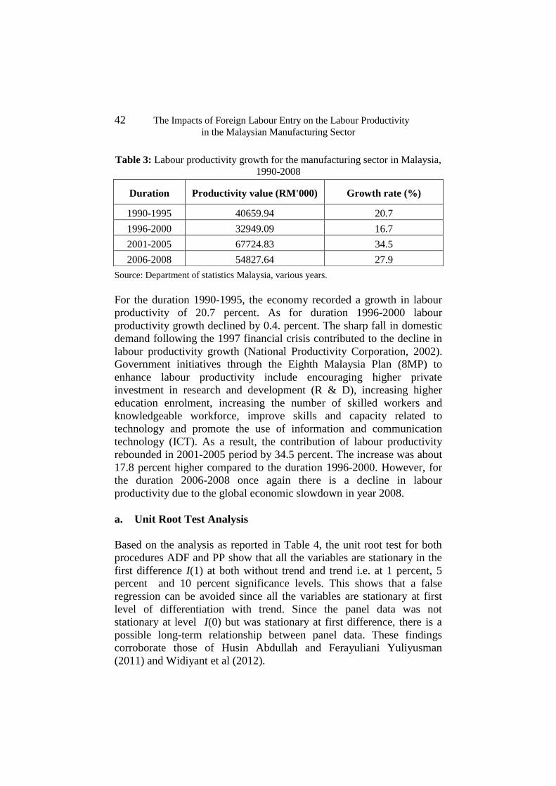
42 The Impacts of Foreign Labour Entry on the Labour Productivity
in the Malaysian Manufacturing Sector
Table 3: Labour productivity growth for the manufacturing sector in Malaysia,
1990-2008
Source: Department of statistics Malaysia, various years.
For the duration 1990-1995, the economy recorded a growth in labour
productivity of 20.7 percent. As for duration 1996-2000 labour
productivity growth declined by 0.4. percent. The sharp fall in domestic
demand following the 1997 financial crisis contributed to the decline in
labour productivity growth (National Productivity Corporation, 2002).
Government initiatives through the Eighth Malaysia Plan (8MP) to
enhance labour productivity include encouraging higher private
investment in research and development (R & D), increasing higher
education enrolment, increasing the number of skilled workers and
knowledgeable workforce, improve skills and capacity related to
technology and promote the use of information and communication
technology (ICT). As a result, the contribution of labour productivity
rebounded in 2001-2005 period by 34.5 percent. The increase was about
17.8 percent higher compared to the duration 1996-2000. However, for
the duration 2006-2008 once again there is a decline in labour
productivity due to the global economic slowdown in year 2008.
a. Unit Root Test Analysis
Based on the analysis as reported in Table 4, the unit root test for both
procedures ADF and PP show that all the variables are stationary in the
first difference I(1) at both without trend and trend i.e. at 1 percent, 5
percent and 10 percent significance levels. This shows that a false
regression can be avoided since all the variables are stationary at first
level of differentiation with trend. Since the panel data was not
stationary at level I(0) but was stationary at first difference, there is a
possible long-term relationship between panel data. These findings
corroborate those of Husin Abdullah and Ferayuliani Yuliyusman
(2011) and Widiyant et al (2012).
Duration Productivity value (RM'000) Growth rate (%)
1990-1995 40659.94 20.7
1996-2000 32949.09 16.7
2001-2005 67724.83 34.5
2006-2008 54827.64 27.9
Journal of Economic Cooperation and Development 43
b. Hausman Test Analysis
Based on the analysis, the results of the Hausman Test for the first
model are shown in Table 5. It was found that for the first model the chi
squared (chi2) is 0.16, Prob> chi2 = 0.9971. This means that Hausman
Test is not significant. The PMG estimation model is more efficient than
the MG. Meanwhile, the results of the Hausman Test for the second
model are shown in Table 6b. The chi squared (chi2) is 0.36 and Prob>
chi2 = 0.9990. Thus, the PMG estimation model is more efficient than
the MG estimation model.
c. Analysis of Dynamic panel data test estimation Pooled Mean
Group (PMG) for First Model
PMG estimation has been conducted and the results from the first PMG
estimation model are shown in Table 5. Results from the first estimation
model using ARDL (0,2,3,0,1) found that in the short term, the error
correction term (ec) is negative 0.19 and is significant at significance
level of 5 percent. The negative ec value reflects the existence of long-
term relationships in the model. In the short term, the results showed
that only the variable KL give significant and positive results in relation
to labour productivity. A 1 percent increase in KL will increase labour
productivity by 0.46 percent. The variable FW, LW, and FDI are
negatively related and do not significantly affect labour productivity.
According Hercowitz et al. (1999) the negative contribution of foreign
and domestic labour on labour productivity growth is only in the short
run. This is because they need to take time to adapt to the labour market
or a new job. FDI inflows into the manufacturing sector in Malaysia
bring with it technology from the country of origin. In the short run,
labour is less able to absorb and apply the technology brought in, which
means that the technology cannot be used efficiently. This tends to
change over time.
In the long run, all variables studied showed significant effects with
labour productivity at the significance level of 1 percent. This is
observable in Table 4 for FW where the coefficient value is positive
0.17. In other words, a 1 percent increase in FW increases labour
productivity by 0.17 percent. The positive effects of foreign labour
supports the findings by Peri (2012) and Kangasniemi et al. (2009). FDI
also positively contributes to labour productivity in the long term with a
44 The Impacts of Foreign Labour Entry on the Labour Productivity
in the Malaysian Manufacturing Sector
0.14 percent increase in productivity with any 1 percent increase in FDI.
Ram and Zhang (2002), who used data from the year 1990 cross-
sectional data, also found the same relationship. The variables LW and
KL also showed the same relationship with coefficients of 1.15 and
0.289. The findings on the variable KL disagrees with the findings in
Zaleha et al (2011). They argued that KL and labour productivity are
inversely related.
d. Analysis of Dynamic Panel Data Test Pooled Mean Group
(PMG) Etimation for the Second Model
In the second estimation model, the findings have been shown in Tables
6a and 6b. Foreign labour and local labour were broken down into two
types of labour by skill type for each type of labour. Foreign and local
labour who work in administrative and professional occupations,
technical and supervisory are classified into skilled labour. While the
labour involved in clerical, general employment and production are
classified unskilled labour. The results from both estimation models
using ARDL (0,0,1,0,0,2,0) found that in the short term, the ec is
negative 0.24 and is significant at 5 percent significance level. The
negative ec value reflects the existence of long-term relationships in the
model studied. In other words, the existence of a long term relationship
between the independent variable and labour productivity in the second
estimation model.
In the short run, the analysis showed that skilled foreign workers
(SkillFW), skilled local labour (SkillLW), unskilled foreign labour
(UnskillFW) and unskilled local labour (UnskillLW) all have negative
but not significant influence on labour productivity. These results
suggest that there is no difference between the productivity of both
labour for skilled and unskilled category in influencing labour
productivity growth. For the category of skilled labour, these findings
are not consistent with the human capital theory where skilled workers
are able to contribute to higher levels of productivity. Level of skills
possessed by the skilled labour are mostly at the most basic level and is
more operations and production oriented, and this may reduce their
influence on the productivity of the organization represented (Rahmah
Ismail et al, 2003) .Besides, variables KL and FDI show positive
influence but are also not significant.

Journal of Economic Cooperation and Development 45
However, in the long run, the study found that all types of labour
according to skill levels indicate relationship with labour productivity
and are all significant at 1 percent significance level. The results
obtained are that SkillFW and SkillLW are positively related to
productivity growth and the values of the coefficient are 0.035 and 0.45
respectively. According Rahmah Ismail et al. (2003), professional
foreign labours are necessary because they can motivate increase in
output. In fact, the recruitment of skilled and experienced,
knowledgeable foreign worker in the manufacturing industry is essential
for smoothing and accelerating the process of transfer of modern
technology. On the other hand, UnskillFW and UnskillLW showed a
negative relationship with productivity growth. This can be seen from
the obtained coefficients of -0.13 and -0.086. The negative coefficient
for the variable UnskillFW and UnskillLW means that a 1 percent
increase of UnskillFW and UnskillLW will reduce labour productivity
by 0.13 percent and 0.086 percent respectively. George Borjas (2006),
using case studies in the United States, concluded that migrant workers
contribute a negative impact on labour productivity of American,
especially those with low skills. Similarly, KL and FDI respectively
relate positively with labour productivity and the coefficients are 0.36
and 0.0085.
5. Conclusions and Suggestions
The study found that overall, in the short run, local and foreign labour
force labour contribute negatively but are both not significant to the
growth of labour productivity. In contrast, in the long run, both have a
positive relationship with labour productivity growth. The labour
productivity increase is a good omen toward achieving a high-income
country status by the year 2020, due to the increase in total output
produced. When broken down by type of labour skill categories, only
migrant labourers and skilled local labour have positive and significant
relationship with labour productivity in the long term. In other words,
foreign and local recruitment of skilled labour is necessary because they
can lead to increase in productivity. Meanwhile, with regard to variable
KL, it was found that in the long run, it has a positive impact on labour
productivity growth of the manufacturing sector. Similarly, the FDI
variable indicated a positive relationship with labour productivity in the
long term. The findings support previous studies which argue that FDI

46 The Impacts of Foreign Labour Entry on the Labour Productivity
in the Malaysian Manufacturing Sector
intensive industries contribute more to productivity than those which are
not FDI intensive ( Thangavelu and Owyong, 2003).
The study concludes that high-skilled foreign workers are needed to help
develop the manufacturing sector in Malaysia. Recruitment of unskilled
foreign labour should be reduced and replaced with the use of local
labour to fill labour shortages. In order to decrease the dependence on
foreign labour, especially unskilled foreign labour, the government has
undertaken several efforts. Among them are efforts to attract expertise
from other countries and Malaysians who are working in other countries
to return home and work in Malaysia to improve the various sectors
especially the R&D sector. These measures should be strengthened
from time to time so that results can be obtained continuously and the
implementation can be more effective. The demand for knowledge
workers, a category that includes senior officials and managers,
professionals, technicians and associate professionals is expected to
increase at an average rate of 2.5 percent per annum (Malaysia, 2006).
The introduction of a minimum wage by the government does not only
benefit local labour, it is also aimed at reducing Malaysia's dependence
on foreign labour especially unskilled foreign labour. Higher minimum
wages lead to increased cost to the employer. Such circumstances would
indirectly force employers to reduce the use of foreign labour and thus
pave the way to greater employment of local labour. Moreover, in
encouraging more local labour into the workforce in labour, especially
in the farming sector, the government is always trying to upgrade
facilities and provide the basic infrastructure including residential estate
(National Productivity Corporation, 2011).
This study also presents a number of steps that can be taken into account
to assist policy makers in designing a strategy to reduce dependence on
foreign labour. The researcher suggests that the policy maker step up
efforts to streamline the recruitment of foreign labour and the levy
system, revise the wage system, and provide better benefits to increase
the chances of retaining local labour in selected sectors. The government
should review the policies, strategies, laws and procedures relating to
the employment and wages of highly skilled foreign expertise of in
select occupations. Firms are also encouraged to implement
productivity-linked salary system. Through innovation and exploitation
of new ideas, added value can be obtained using the same human capital
Journal of Economic Cooperation and Development 47
and the same amount of other resources. Investment in science, research
and education can also serve as an engine of innovation for the
economy.
FDI will be continue to be a catalyst to improve the R&D ability and as
a source of technology transfer. Private sector actors are urged to forge
strategic alliances with foreign partners to ensure that their R&D
activities are not out of touch with the outside world. The government
should continue to identify and provide assistance to multinational
companies with R&D capabilities in strategic areas to invest in
Malaysia. In addition, the incentive mechanism for FDI should be
revised to give priority to those with new, updated R&D capabilities and
with value-added to be located in Malaysia.
48 The Impacts of Foreign Labour Entry on the Labour Productivity
in the Malaysian Manufacturing Sector
References
Aliya Rosa., Rahmah Ismail., & Noorasiah Sulaiman,.(2012).
Globalisation and Labour Productivity in the Malaysian Manufacturing
Sector. Review of Economics & Finance, 2, 76-86.
Borjas, G. J. (1993). Immigration Policy, National Origin, and
Immigrant Skills: A Comparison of Canada and the United States.
National Bureau of Economic Research. No. 3691
Borjas, G. J. (2006). Native internal migration and the labour market
impact of immigration. Journal of Human Resources, 41(2), 221-258
Chia, S.Y. (2011).Foreign labour in Singapore: trends, policies, impact
and challenge. Philippine Institute for Development Studies, No.2011-
24.
Chuang, Y. C., & Lin, C. M. (1999). Foreign direct investment, R&D
and spillover efficiency: Evidence from Taiwan's manufacturing firms.
The Journal of Development Studies, 35(4), 117-137.
Hale, G., & Long, C. X. (2006). What determines technological
spillovers of foreign direct investment: Evidence from China. Economic
Growth Center, Yale University.
Hausman, J. A. (1978). Specification tests in econometrics.
Econometrica: Journal of the Econometric Society, 1251-1271.
Hercowitz, Z., Lavi, Y., & Melnick. (1999). The Impact of
Macroeconomic Factors on Productivity in Israel, 1960-96. Bank of
Israel Economic Review 72: 103-124
Huber, P., Landesmann, M., Robinson, C., & Stehrer, R. (2010).
Migrants skills and productivity: A European Perspective. National
Institute Economic Review, 213(1), R20-R34.
Husin Abdullah & Ferayuliani Yuliyusman. (2011). The effects of
economic freedom on economic growth: Empirical Study in Indonesia,
Hong Kong, Malaysia, Singapore and the United States. Proceeding
PERKEM VI, jilid 1 (2011) 410 – 423.

Journal of Economic Cooperation and Development 49
Ishak Yussof & Nor Aini Haji Idris (2009). Policy and strategy of
economic development of Malaysia: An assessment of the economy
towards balanced development, edited by Nor Aini Haji Idris dan Ishak
Yussof. Bangi: Printed by University Kebangsaan Malaysia.
Prime Minister's Department of Malaysia.Economics Transformations
Program Report (ETP), (2012). Kuala Lumpur. Printed by National
Malaysia.
Department of Statistics Malaysia. Malaysia Manufacturing Industries
Survey Report, various years. Kuala Lumpur. Printed by National
Malaysia.
Kangasniemi, M., Ivars, M. M., Robinson, C., & Martínez, L. S. (2009).
The economic impact of migration: Productivity analysis for Spain and
the United Kingdom. Documentos de trabajo (Fundación BBVA), (10), 1
Llull, J (2008). The impact of immigration on productivity. Center for
Monetary and Financial Studies (CEMFI), No. 0802 Malaysia (1996).
Seven Malaysia Plan , 1996-2000. Kuala Lumpur: Printed by National
Malaysia.
Malaysia (2006). Ninth Malaysia Plan, 2006-2010. Kuala Lumpur:
Printed by National Malaysia.
Malaysia (2011). Ten Malaysia Plan , 2011-2015. Kuala Lumpur:
Printed by National Malaysia.
Widiyanti, M. (2012). Monetary with Interest Rate Policy and Impact on
Prices: Empirical Evidence from Malaysia. Proceedings PERKEM VII,
jilid 1 (2012) 91 – 100.
Mohammad Sharif Karimi & Zulkormain Yusop (2009).FDI and
economic Growth in Malaysia.Faculty of Economics and Management,
University Putra Malaysia.
Malaysia Productivity Corporation .(2011). Productivity Report. Kuala
Lumpur: Printed by National Malaysia.
50 The Impacts of Foreign Labour Entry on the Labour Productivity
in the Malaysian Manufacturing Sector
Malaysia Productivity Corporation. (2013). Productivity Report. Kuala
Lumpur: Printed by National Malaysia.
Peri, G. (2012). The effect of immigration on productivity: Evidence
from US states. Review of Economics and Statistics, 94(1), 348-358.
Pesaran, M. H., Shin, Y., & Smith, R. J. (1999).Bounds Testing
Approaches to the Analysis Long Run Relationship. Unpublished
Manuscript. University of Cambridge.(http// www.econ.cam.ac.uk/
faculty pesaran.
Preibisch, K. L. (2007). Local produce, foreign labour: Labour mobility
programs and global trade competitiveness in Canada. Rural Sociology,
72(3), 418-449.
Pritchard, R. D. (1995). Productivity measurement and improvement:
Organizational case studies. Praegar.Publisher Prokopenko, J. (1987).
Productivity management: A Practical Handbook. Geneva:ILO
Rosario-Braid, F. (1983). Communication strategies for productivity
improvement Tokyo: Asian Productivity Organization.
Rahmah Ismail, Nasri Bachtiar, Zulkifly Osman & Zulridah Mohd Noor
(2003). The role of foreign labour to output growth, employment
opportunities and wages in the manufacturing sector in Malaysia.
Journal of Economics Malaysia 37:103-128.
Ram, R., & Zhang, K. H. (2002).Foreign direct investment and
economic growth: Evidence from Cross‐Country data for the 1990s.
Economic Development and Cultural Change, 51(1), 205-215.
Sahar, M .(2002). Labour productivity: An important business strategy
in manufacturing. Integrated Manufacturing Systems, 13(6),435-438
Salim, R. A., & Bloch, H. (2009).Does foreign direct investment lead to
productivity spillovers? Firm level evidence from Indonesia.World
Development, 37(12), 1861-1876.

Journal of Economic Cooperation and Development 51
Thangavelu, S. M., & Owyong, D. T. (2003).The impact of export
growth and scale economies on productivity in Singapore's
manufacturing industries. Journal of Economic Studies, 30(6), 623-635
Zaleha M.N., Noraini I., Rusmawati S., & Suhaila A.J. (2011).The
Impact of foreign workers on labour productivity in Malaysia
manufacturing sector. Int. Journal of Economics and Management
5(1): 169-178.

52 The Impacts of Foreign Labour Entry on the Labour Productivity
in the Malaysian Manufacturing Sector
Table 4: Results for Unit root test ADF and PP
Variable ADF Philips Perron (PP)
Without Trend Trend Without Trend Trend
Level
InLW -1.6890 -2.0667 -1.7100 1.8953
(0.2300) (0.2369) (0.2299) (0.2370)
InFW -0.5659 -1.7679 -0.2466 -1.6063
(0.1933) (0.2164) (0.1932) (0.2064)
lnSkillLW -2.6450 -3.7204 -2.6445 -3.7200
(0.2131) (0.2600) (0.2100) (0.2555)
lnSkillFW -3.0741 -3.6774 -3.8573 -4.5720
(0.2436) (0.2524) (0.2440) (0.2500)
lnUnSkillLW -1.3650 1.7900 -1.4161 1.8000
(0.1700) (0.1744) (0.1672) (0.1744)
lnUnskillFW 0.3158 -2.0631 0.8032 -1.9858
(0.0881) (0.1774) (0.0900) (0.1774)
lnKL -2.4111 -2.0066 -2.3556 -1.9332
(0.1850) (0.2313) (0.1845) (0.2310)
lnFDI -4.4193 -4.2835 -4.4202 -4.2838
(0.2490) (0.2578) (0.2491) (0.2577)
Difference
Without Trend Trend Without Trend Trend
InLW -7.5267 -10.8000 -6.6781 12.1981
(0.1886)*** (0.1420)*** (0.1890)*** (0.1410)***
InFW -5.5500 -6.3010 -5.5400 -7.8247
(0.2413)** (0.2414)** (0.2403)** (0.2424)***
lnSkillLW -6.7111 -6.5311 -12.3400 -16.0802
(0.2235)*** (0.2310)** (0.2235)*** (0.2206)**
lnSkillFW -7.0468 -8.1492 -7.1000 -8.6363
(0.2709)*** (0.2715)*** (0.2710)*** (0.2710)***
lnUnSkillLW -4.0310 -4.0861 -4.0312 -3.2977
(0.2578)* (0.2650)* (0.2577)* (0.2648)*
lnUnskillFW -4.1910 -4.5616 -2.6666 -3.7104
(0.2673)* (0.2940)** (0.2700)* (0.2939)**
lnKL -4.8425 -4.4287 -5.0787 -12.1316
(0.2536)** (0.5767)* (0.2540)* (0.2528)***
lnFDI -6.9469 -6.7336 -16.9683 -18.3393
(0.2196)*** (0.2269)** (0.2197)*** (0.2270)**
Note: ***, **, and *is significant at 1% , 5%, and 10% significance level. Upper value
is the coefficient value, the value in bracket is the standard deviation.

Journal of Economic Cooperation and Development 53
Table 5: Results of Labour productivity estimation using first model
Pooled Mean Group (PMG).
DEPENDENT VARIABLE:
Productivity Growth (In Y/L)
Model 01:
ARDL (0,2,3,0,1)
Short term effect
∆lnFW -0.0037
(0.0573)
∆lnLW -0.3251
(0.418)
∆lnKL 0.4552
(0.1046)***
∆lnFDI -0.001
(0.0167)
Constant 0.5745
(0.2266)**
Error Correction Term (ec) -0.1861
(0.043)**
Long term effect
lnFW 0.1711
(0.0516)***
lnLW 1.1519
(0.3374)***
lnKL 0.2894
(0.0547)***
lnFDI 0.1384
(0.0192)***
Hausman Test chi2(4)= (b-B)'[(V_b-V_B)^(-1)](b-B)
= 0.16
Prob>chi2 =0.9971
Note: Lag order is chosen based on AIC (Akaine Information Criteria).*** Significant
at 1% significance level, ** Significant at 5% significance level and *Significant at
10% significance level. Upper value is the coefficient value, the value in bracket is
the standard deviation.
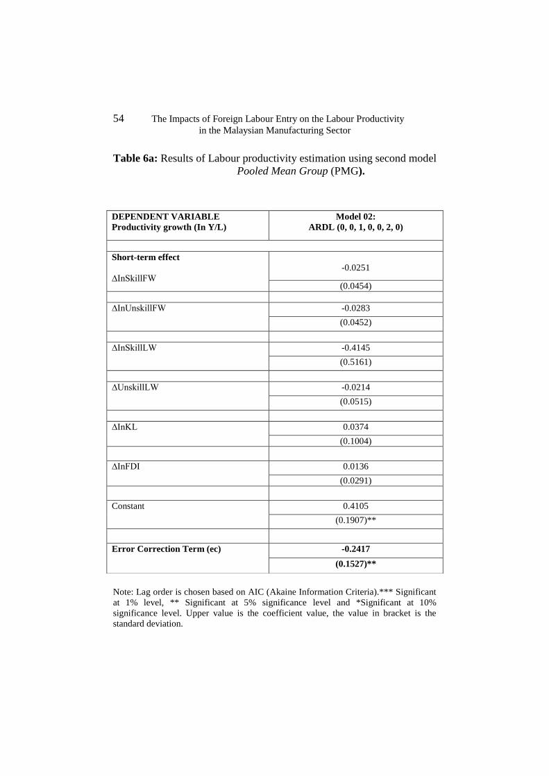
54 The Impacts of Foreign Labour Entry on the Labour Productivity
in the Malaysian Manufacturing Sector
Table 6a: Results of Labour productivity estimation using second model
Pooled Mean Group (PMG).
Note: Lag order is chosen based on AIC (Akaine Information Criteria).*** Significant
at 1% level, ** Significant at 5% significance level and *Significant at 10%
significance level. Upper value is the coefficient value, the value in bracket is the
standard deviation.
DEPENDENT VARIABLE
Productivity growth (In Y/L)
Model 02:
ARDL (0, 0, 1, 0, 0, 2, 0)
Short-term effect
∆InSkillFW
-0.0251
(0.0454)
∆InUnskillFW -0.0283
(0.0452)
∆InSkillLW -0.4145
(0.5161)
∆UnskillLW -0.0214
(0.0515)
∆InKL 0.0374
(0.1004)
∆InFDI 0.0136
(0.0291)
Constant 0.4105
(0.1907)**
Error Correction Term (ec) -0.2417
(0.1527)**

Journal of Economic Cooperation and Development 55
Table 6b: Results of Labour productivity estimation using second
model Pooled Mean Group (PMG)
Note: Lag order is chosen based on AIC (Akaine Information Criteria).*** Significant
at 1% level, ** Significant at 5% significance level and *Significant at 10%
significance level. Upper value is the coefficient value, the value in bracket is the
standard deviation.
DEPENDENT VARIABLE
Productivity Gowth (In Y/L)
Model 02:
ARDL (0,0,1,0,0,2,0)
Long term effect
InSkillFW 0.0345
(0.0068)***
InUnskillFW -0.125
(0.0360)***
InSkillLW 0.447
(0.0103)***
InUnskillLW -0.0863
(0.0151)***
InKL 0.3614
(0.0105)***
InFDI 0.0085
(0.0028)**
Hausman Test chi2(6) =(b-B)'[(V_b-V_B)^(-1)](b-B)
=0.38
Prob>chi2=0.9990


Journal of Economic Cooperation and Development, 37, 3 (2016), 57-86
The Real Effect of Government Debt:
Evidence from the Malaysian Economy
Siti Nurazira Mohd Daud
The results demonstrate that there is a long-run relationship between federal
government debt and economic growth in Malaysia. In addition, our findings
are of great interest since there is evidence of a non-linear relationship
between the federal government debt and economic growth, which suggests
the optimal level of debt that the government should hold. Hence, the
accumulation of federal government debt is positively associated with
Malaysia’s economic growth up to an optimal level. While an additional
increase in federal government debt beyond the optimal level has inversely
contributed to the Malaysian economy.
1. Introduction
There are several lessons to be learnt from the recent sovereign debt
crisis that has affected most of the European economies. A rise in public
debt and country-specific problems are among the factors behind the
European Financial Crisis. Ireland is facing a banking crisis while Spain
is experiencing a housing bubble. In addition, Greece, Italy and Portugal
are involved in fiscal mismanagement. Thus, they have drawn their
economies into sovereign debt crises and are still in the process of
recovery four years after the crisis erupted in 2008. On the other hand,
current development shows that Japan, Greece, Italy, Portugal and
Ireland are among the top-listed countries with very high levels of public
debt (IMF 2012). As at the end of 2011, Japan held a public debt of
about 229.77 per cent of gross domestic product (GDP) and this was
expected to hit almost 240 per cent of its growth. In addition, Greece,
Italy, Portugal and Ireland held public debts (as percentages of GDP) of
about 160.81 per cent, 120.11 per cent, 106.79 per cent and 104.95 per
cent respectively. Furthermore, in response to this issue, the
Organisation for Economic Cooperation and Development (OECD) has
Faculty of Economics & Muamalat, Universiti Sains Islam Malaysia
Email: [email protected]
58 The Real Effect of Government Debt:
Evidence from the Malaysian Economy
called on countries to cut their public debts to prudent levels of around
50 per cent of GDP in order to cope with future challenges including
health, long-term care and pensions.2
Looking at the roots of the problem, it can be seen that persistent large
deficits, used primarily to finance public sector operating expenses, have
resulted in high ratios of debt to GDP, thus driving Greece and other
European countries into debt overhang problems. In the midst of this
phenomenon, some developing countries are showing signs or
symptoms of the debt overhang problem; this highlights the question of
whether government debt has benefited economies (Cecchetti, Mohanty
and Zampolli 2011; Baum, Checherita-Westphal and Rother 2012;
Presbitero 2010; Caner, Grennes and Koehler-Geib 2010). Thus has
underlined the urgency of investigating the issue of the heavy stock of
public debt in developing economies, since neither developed nor
developing countries are immune to the public debt sustainability issue.
Malaysia, a small open economy, has recorded a fiscal deficit position
since its independence in 1957 except for the period 1993-1997.
Furthermore, the country has recorded 13 consecutive years of fiscal
deficits since the year 1997. This condition was leading Malaysia to
accumulate a stock of indebtedness regardless of domestic or
international capital markets since, by continuing to run budget deficits,
the country would have a high stock of debt (as depicted in Appendix
1). In addition, the federal government debt was financed from domestic
and foreign funding, which constituted approximately 96.2 per cent and
3.8 per cent of the gross borrowing respectively.3 As at the end of 2011,
total federal government debt was recorded at RM 455,745 million,
which is equivalent to 53.8 per cent of Gross Domestic Product (GDP)
(Malaysia Economic Planning Unit 2011). This position has already
been reached and is slightly higher than the prudent cut-off point of
public debt-holding that has been set for developed economies.
However, no one size fits all. This highlighted the importance of
2 Furthermore, the European Union has set a ceiling for public debt at 60 per cent of
GDP. By the same token, OECD highlights the importance of macro prudential
supervision on an individual-country basis. 3 Meanwhile, the federal government financing came mainly from domestic sources
through the issuance of Malaysian Government Securities (MGS) and Government
Investment Issues (GIIs) where the major shareholders were Employee Provident Fund
(EPF), foreign investors, banking institutions and insurance companies.
Journal of Economic Cooperation and Development 59
analysis on a country-by-country basis before it was too late and the
country had already passed its optimal level, becoming trapped in a debt
overhang situation, being in default and, to a lesser extent, witnessing
the eruption of a sovereign debt crisis.
In principle, if borrowing has been allocated efficiently, a country will
benefit from it since debt financing of public spending can make a
positive contribution to productive investment and ultimately to
economic growth (Miller and Foster 2012). In contrast, a country with
high levels of debt will face the probability of a debt overhang problem,
to a lesser extent, or default or bankruptcy. As such, the increasing level
of government indebtedness raises the issue of the effectiveness of the
fiscal policy formulated by the government. Furthermore, it leads to the
issue of whether the borrowing is efficiently and productively allocated
to the economy through development projects which in return will
generate sustainable economic growth.4
A country that accumulates large stock of debt and could affect the
ability to repay its debts is more likely involved in a debt overhang
situation. There is limited study conducted to investigate the effect of
debt overhang on various economies. Recent study conducted by
Reinhart et al. 2012, identify 26 public debt overhang episodes in 22
advanced economies since the early 1800s. The study found that growth
effects are significant even in the many episodes where debtor countries
were able to secure continual access to capital markets at relatively low real
interest rates. On the other spectrum, Brown and Lane (2011) conduct a
study to assess the effect of debt overhang to economic activity in
Emerging Europe countries. Debt overhang could be a threat to activity
in the tradable sector in the more advanced economies of the region. In
addition, the debt overhang emerge at different levels of indebtedness
depending on the country characteristics namely institution, policies and
4 The highest deficit was recorded in 2009 and was due to the global economic
slowdown as the external sector collapsed and the business community remained
cautious and risk-averse. Weak private investment, sluggish exports performance and
higher expenditure incurred are due to the implementation of the stimulus packages,
resulting in a weak financial position in the fiscal position (Malaysia Economic
Planning Unit 2009).

60 The Real Effect of Government Debt:
Evidence from the Malaysian Economy
access to private capital (Cordella et al. 2005). Sound institutions can
probably affect the ability to service debt in times of crisis. As such,
with limited but growing study, the effect of debt overhang situation
might differ depending on the economies.
As a consequence, the increasing level of the stock of government debt
has raised concerns and leads to the question of whether a country with
high levels of government debt is still sustainable. Furthermore, this
problem could threaten the developing economies, especially their
banking sectors, in the event of sovereign debt crises. Thus, this
situation has intensified interest and drawn attention to the long-lasting
implications of policy action for the country’s government debt position.
A real picture of Malaysia’s public debt position is important for policy
formulation as well as for investors’ ability to strategize their investment
decisions. Considering the growth in the literature on developed
countries, an attempt to investigate Malaysia’s public debt position is
feasible since, as a small open economy, Malaysia also faces a high risk
of vulnerability and uncertainty in its economy. Focusing on a long-
horizon return, the objective of this paper is to analyze the real effect of
government debt on Malaysia’s economy. This study is a contribution to
the literature on the Malaysian government’s debt position after a long
episode of fiscal deficits. Thus, this study attempts to fill this gap in the
literature. The paper is laid out as follows. Section II offers a brief
overview of the literature on external debt. Section III outlines the data
and methodology, while the empirical results are presented in section
IV. Section V concludes the paper.
2. Theoretical and empirical evidence
Over the past decades, academics and policy-makers have shown a
consistent interest in investigating and developing the theory on the link
between debt and economic growth. However, a limited but growing
number of studies have been examining the role of public debt in a
country’s economic growth.5 The discussion on the impact of public
debt on a country’s growth has produced a single conclusion on the
adverse impact of public debt on growth (Modigliani 1961; Adam and
Bevan 2005; Aizenman et al. 2007). Based on the aggregate model
5 On the other hand, there is a vast amount of literature focusing on the impact of
external debt in generating countries’ economic growth.

Journal of Economic Cooperation and Development 61
developed by Modigliani (1961), the accumulation of government debt
will have a positive impact on growth if the increase in debt is
accompanied by government expenditure on productive public capital
formation. In other words, the debt will benefit the economy if it is
capable of generating a stream of real income for future generations and
vice versa (Modigliani 1961). In addition, Modigliani stated that holding
too much public debt will affect the country through the crowding-out
effect, which will lead to the debt overhang problem, as explained by
Krugman (1988). On the other hand, by setting up a simple overlapping
generation (OLG) model of savings, Adam and Bevan (2005) found
evidence of interactive effects between deficits and debt stock, with high
debt stock exacerbating the adverse consequences of high deficits.
Furthermore, the fiscal deficits would be growth-enhancing if financed by
limited seigniorage, growth-inhibiting if financed by domestic debt, and
have an opposite flow and stock effect if financed by external loans. In
addition, Aizenman et al. (2007) examined the optimal public investment
and fiscal policy for countries subject to binding on tax and debt
capacities. They found that the public debt-to-GDP ratio should be held
constant in the economy, adding that public sector borrowing to finance
the accumulation of public capital goods may allow the economy to reach
a long-run optimal growth path faster (Aizenman et al. 2007).
Several empirical works have focused on the impact of public debt on a
country’s economic growth, while proposing a non-linear analysis
(Reinhart and Rogoff 2010; Pattillo 2004; Baum et al. 2012; Cecchetti et
al. 2012; Presbitero 2010; Schclarek 2004). Most of the literature found
that the tipping point of government debt should be held at around 64
per cent to 100 per cent of GDP depending on the size and the
development stage of the economy. In particular, Reinhart and Rogoff
(2010) conducted a study on 20 developed countries over the period
1790-2009 to investigate the relationship between public debt and long-
term real GDP growth. The findings suggest that the relationship
between public debt and economic growth is relatively weak below the
threshold of 90 per cent of GDP; however, above the 90 per cent level
the median growth rate falls by one per cent. By the same token,
Checherita and Rother (2010) examined the impact of government debt
on economic growth in twelve Euro-area countries for a period spanning
about 40 years from 1970 and found a non-linear impact of debt with 90
to 100 per cent of GDP estimated as the optimal level. On the other

62 The Real Effect of Government Debt:
Evidence from the Malaysian Economy
hand, recent studies conducted for almost the same sample, for the
period 1990-2010, suggest that the short-run impact of debt on growth is
positively and statistically significant up to 67 per cent debt to GDP
(Baum et al. 2012). Meanwhile, according to Baum et al. (2012), beyond
the limits the positive impact of government debt decreases to around
zero and loses its significant impact on economic growth. However, no
robust evidence on the relationship between government debt and
economic growth has been found for 24 industrial countries (Schclarek
2004). In addition, results from a dataset of 18 OECD countries over the
period 1980-2010 support the view that, beyond 85 per cent debt to
GDP, debt is a drag on growth (Cecchetti et al. 2012). Meanwhile,
Presbitero (2010) complemented the existing studies by focusing on the
developing countries. Over the period 1990-2007, the results show that
public debt has a negative impact on output growth up to a threshold of
90 per cent of GDP; beyond this level, its effect becomes irrelevant. An
interesting study by Caner et al. (2010) estimates the threshold debt
levels based on annual datasets of 101 developing and developing
countries from 1980 to 2008. The results established a threshold of 77
per cent public debt-to-GDP ratio. Beyond the threshold level, each
additional percentage point of debt costs 0.017 percentage points of
annual real growth. In addition, results for a sample of emerging
economies are even more pronounced with the estimated thresholds
found to be at 64 per cent debt-to-GDP ratio; above the threshold level
each additional percentage point of public debt amounts to 0.02
percentage points. Thus, inspired by the notion that no one size fits all,
this paper will contribute to the literature by focusing on an individual
developing country, namely Malaysia.
3. Model, Method and Data
A detailed analysis of the effect of federal government debt on
Malaysia’s economic growth will provide evidence on the real scenario
of Malaysia’s federal government debt position. In addition, with the
application of several econometric procedures, the optimal level of
public debt that the country should hold will be estimated. Thus, to
investigate whether the federal government has contributed to economic
growth, the basic growth model to be estimated is
ttt εβXY 0 (1)
Journal of Economic Cooperation and Development 63
where Y is the dependent variable, X is k-vector of regressors, and the
subscripts t =1,….,T identify the time dimensions. Y represents the real
GDP per capita and X includes investment rate, labour force rate and
federal government debt, while t represent the error term. The real GDP
per capita (dependent variable) is a proxy of economic growth. In
addition, the independent variables include investment rate, labour force
rate and federal government debt to represent the rates of growth of
factor inputs in the production function, and openness captures for
government policy. This paper also estimates the direct link between
federal government debt and investment rate to provide an additional
insight into the effect of federal government debt on economic growth
via capital accumulation. The estimated investment model is
ttt XI 0 (2)
I represents the investment rate while X is labour force, openness and
federal government debt. The investment rate represents the growth of
the economy, labour force rate and federal government debt represent
the rates of growth of factor inputs in the production function, and
openness represents the government policy. Since the observations are
on a quarterly basis, for the maximum order of the lags in the ARDL
model, a lag order of 4 is chosen.
The procedure starts with the Ordinary Least Squares estimation as a
benchmark for the analysis. Next, the analysis proceeds with the
cointegration tests. The Autoregressive Distributed Lag (ARDL)
cointegration bound test developed by Pesaran et al. (2001) will be
employed. The bound test developed by Pesaran et al. (2001) is the
Wald test (F-statistic version of the bound testing approaches) for the
lagged level variables in the right-hand side of an Unrestricted Error
Correction Model (UECM). This procedure involved two stages before
the long-run relationship could be established. In addition, the null
hypothesis of a non-cointegrating relation (Ho: δ1= δ2= δ3=…= δn = 0) is
tested by performing a joint significance test on the lagged level
variables. The first stage of the ARDL approach involved the F-test in
which the asymptotic distribution of the F-statistic is non-standard under
the null hypothesis of no cointegrating relationship between the
examined variables, irrespective of whether the explanatory variables

64 The Real Effect of Government Debt:
Evidence from the Malaysian Economy
are purely I(0) or I(1). Under the conventional levels of significance
such as 10 per cent, 5 per cent and 1 per cent, if the statistic from a Wald
test falls outside the critical bounds value (lower and upper values), a
conclusive inference can be made without considering the order of
integration of the explanatory variables. If the F-statistic exceeds the
upper critical bound, the null hypothesis of no cointegrating relationship
can be rejected. However, if the test statistic (F-statistic) falls below the
lower critical bound, then the null of non-cointegration cannot be
rejected. If the F-statistic falls between the upper and lower bounds, a
conclusive inference cannot be made. Next, the second stage of the
ARDL approach involves an estimation of the coefficients on the long-
run cointegrating relationship and the corresponding error correction
model. The lagged error correction term (et-1) derived from the error
correction model is an important element in the dynamics of the
cointegrated system as it allows for adjustment back to the long-term
equilibrium relationship given a deviation from the last year.
In addition, in order to gather as much as information as possible on the
effect of the federal government debt on Malaysia’s economic growth,
this paper also employs a causality test which is an extension of the
Granger causality test that applies the bootstrapping method with
endogenous lag length proposed by Hacker and Hatemi-J (2010). The
causal relationship between federal government debt and other
economic variables will provide evidence on the impact of federal
government debt on the economy. As such, this analysis should at least
provide some indication of the impact of the current implemented
policy. A standard Granger causality test on the first difference is
performed to find the direction of causality. The Granger test is
performed on
itit
n
i
i GDPFGDFGD 1
1
(3)
itit
n
i
i FGDGDPGDP 1
1
(4)
itit
n
i
i GDPDEFDEF 1
1
(5)

Journal of Economic Cooperation and Development 65
itit
n
i
i DEFGDPGDP 1
1
(6)
itit
n
i
i FGDINVINV 1
1
(7)
itit
n
i
i INVFGDFGD 1
1
(8)
itit
n
i
i DEFINVINV 1
1
(9)
itit
n
i
i INVDEFDEF 1
1
(10)
where GDP represents the real GDP per capita and FGD signifies the
federal government debt. In addition, the INV and DEF represent the
investment rate and federal government deficits respectively. In standard
procedure when applying the Granger causality test, the lag length is
assumed to be known beforehand where the preselection of the lag order
may affect the distribution of the test statistics. Thus, Hacker and
Hatemi-J (2010) suggests endogenously determining the lag length
choice including the use of the bootstrapping method. Furthermore, the
bootstrapping method appears to have better size properties, seems to be
robust to the existence of autoregressive conditional heteroscedasticity
(ARCH), and appears to have more power compared to the asymptotic
test for the same actual size (Hacker and Hatemi-J 2010).6
Next, this paper employs the test proposed by Hansen (2000) which
tests the null hypothesis of a linear regression against a threshold
regression analysis. In the form of the thresholds model,
ttt xy '
1 tq (11)
titt xy '
2 tq (12)
6 Thanks to Professor Abdulnasser Hatemi-J and Scott Hacker for the GAUSS routine.
66 The Real Effect of Government Debt:
Evidence from the Malaysian Economy
where tq is the threshold variable, which is federal government debt. In
addition, the threshold variable could be part of the regressors and it is
used to split the sample into two regimes. Meanwhile ty is economic
growth measured by real GDP per capita. tx is 1p vector of
independent variables which include investment rate, openness and
federal government debt, and t is a regression error.
Hansen (2000) has developed a threshold model estimator that considers
the least squares estimations. Furthermore, by providing an asymptotic
simulation test of the null of linearity against the alternative of a
threshold, this method also computed a confidence interval by inverting
the likelihood ratio statistics. Hansen (2000) also proposes an F-test
bootstrap (heteroscedasticity-consistent) procedure to test the null of
linearity. Since the threshold value is not identified under the null, the
p-values are computed by a fixed bootstrap method. The sample consists
of economics data from the period 1996Q1-2011Q4. The data are
collected from the IMF/IFS statistics and the Monthly Bulletin of the
Central Bank of Malaysia. Details of the variables are attached in
Appendix 5.
4. Results and discussion
4.1 Descriptive analysis
Table 1 provides descriptive statistics on the main variables employed in
this study. The variables include real GDP per capita, labour force,
investment, openness, federal government debt and federal government
expenditure. The descriptive statistics consist of mean, standard
deviation, maximum values and minimum values. Table 1 shows that
there are substantial variations for all variables. The real GDP per capita
ranges from RM2,785 to RM7,090 with a mean value of RM4,454. In
addition, the labour force and investment show small variations with
lower values of standard deviation, which indicates the dispersion from
the mean. Meanwhile the openness variable ranges from RM95,889 to
RM330,817, with a mean of RM206,075. By the same token, with a
significant variation indicated by its standard deviation of RM108,776,
the mean value of federal government debt is RM210,478.

Journal of Economic Cooperation and Development 67
Table 1. Descriptive Statistics
Mean Standard Deviation
Min Max
Real GDP per capita 4,454 1,110 2,785 7,090
Labour force 10,253 1,095 8,469 12,730
Investment 27,075 5,988 15,189 39,019
Openness 206,238 71,614 95,889 330,817
Federal government debt 210,478 108,776 83,533 456,127
Note: All figures are in RM Million.
The investigation starts by analyzing the composition of Malaysia’s
government debt. Figure 1 shows the composition of federal government
debt over the period 1970-2012. The figure shows a stable pattern with
the domestic debt accounting for about 85 per cent of total federal
government debt in 1970, increasing to 96 per cent in 2011. In addition,
the borrowing is funded from domestic financial institutions in
Malaysia, including banks, financial institutions and social security
institutions.
Figure 1. The composition of Malaysia Federal Government Debt
0
50,000
100,000
150,000
200,000
250,000
300,000
350,000
400,000
450,000
19
70
19
73
19
76
19
79
19
82
19
85
19
88
19
91
19
94
19
97
20
00
20
03
20
06
20
09
RM
Mill
ion
Year
Domestic debt External debt

68 The Real Effect of Government Debt:
Evidence from the Malaysian Economy
In addition, about 63 per cent and 25 per cent are in the form of
government securities and government investment issues (GII’s)
respectively (as at the end of 2011). Furthermore, the maturity of the
government debt is mainly seen over the maturity periods of 6 to 10
years and 4 to 5 years, covering 38 per cent and 29 per cent respectively
of the total government securities debt.
4.2 Empirical analysis
The empirical analysis of this paper starts by estimating a standard
ordinary least squares test on the standard baseline debt-growth model to
establish a reference point. The results are shown in Table 2. By
following the general-to-specific methodology, the results show an
estimation of a model where the real GDP per capita and investment
signify the economic growth. The estimated model of real GDP per
capita as the dependent variable is shown in columns (1) to (5), while
columns (6) to (10) show the results of the estimates where investment
proxy is the dependent variable. The results in columns (1), (2) and (3)
show an insignificant effect of federal government debt on the country’s
economic growth (which is proxied by the real GDP per capita as the
dependent variable). However, estimates that only consider federal
government debt as the independent variable reveal a positive and
significant effect (at 5 per cent significance level) on the country’s
economic growth.
On the other hand, with the investment rate variable representing the
country’s growth, there are positive and significant (at 5 per cent
significance level) effects of federal government debt on the country’s
growth, as depicted in columns (6), (7) and (10). Meanwhile, the results
also reveal a positive and significant (at 5 per cent significance level)
effect of trade openness in explaining Malaysia’s economic growth, as
shown in columns (1) to (3). In addition, we try to include the federal
government debt squared in columns (3) and (8) to investigate the
potential of the non-linear effect or debt-Laffer curve relationship.
Columns (3) and (8) demonstrate that the federal government debt has a
significant effect on the country’s economic growth. In addition, the
federal government debt ^2 variable is significant at 5 per cent
significance level, with a negative effect on the growth rate of the
country’s income. This may implies evidence of an inverted-U-shaped
relationship in the federal government debt-growth model. The inverted-

Journal of Economic Cooperation and Development 69
U relationship explains that an increase in debt stock has a positive
effect on economic growth until it achieves its optimal level (up to a
certain level). Beyond the threshold level, an increase in the stock of
indebtedness is associated with a negative effect on economic growth.
The negative effect could be related in cases where it has not been
efficiently allocated to investment and if there is too much debt-holding
that might squeeze the investment through debt repayment. In contrast,
the results show that the federal government deficit plays an
insignificant role in explaining the variability in economic growth.
However, these results should be interpreted with caution since the
diagnostic test shows a sign of bias where the results may be suffering
from major econometrics problems including serial correlation,
functional form and heteroscedasticity problems.
We proceed by estimating equations (1) and (2) with cointegration
technique to examine the long-run cointegration relationship between
economic growth and federal government debt with the inclusion of
other explanatory variables.

70 T
he
Rea
l E
ffec
t of
Gover
nm
ent
Deb
t:
Evid
ence
fro
m t
he
Mal
aysi
an E
con
om
y
Ta
ble
2.
Res
ult
s O
f O
rdin
ary L
east
Squar
es E
stim
atio
n o
n t
he
Impac
t of
Fed
eral
Go
ver
nm
ent
Deb
t an
d D
efic
its
to t
he
Eco
nom
y
R
eal
GD
P P
er C
ap
ita a
s th
e D
ep
en
den
t V
ari
ab
le
Inv
estm
en
t as
the
Dep
end
en
t V
ari
ab
le
(1
) (2
) (3
) (4
) (5
) (6
) (7
) (8
) (9
) (1
0)
ln (
Inves
tmen
t)
0.2
34
(0.0
59
)*
0.2
79
(0.0
58
)*
0.2
15
(0.0
60
)*
0.3
100
(0.0
57
)*
ln (
Lab
ou
r)
-1.3
21
(0.4
75
)8
-1.3
18
(0.4
72
)*
-0.8
50
(0.4
83
)**
-0.6
74
(0.2
57
)*
-1
.18
9
(1.0
46
) -1
.23
3
(1.0
49
) 0
.15
5
(1.0
51
) 0
.77
1
(0.5
73
)
ln (
Tra
de
Op
enn
ess)
0
.61
1
(0.0
80
)*
0.6
10
(0.0
79
)*
0.5
46
(0.0
79
)*
0.6
68
(0.0
73
)
0.0
10
(0.1
78
) 0
.01
7
(0.1
78
) -0
.14
8
(0.1
72
) 0
.19
1
(0.1
63
)
ln (
Fed
eral
go
ver
nm
ent
deb
t)
0.1
79
(0.1
11
) 0
.17
3
(0.1
11
) 0
.17
5
(0.1
05
)
0.4
08
(0.0
35
)*
0.5
27
(0.2
38
)*
0.5
19
(0.2
39
)*
0.4
13
(0.2
22
)
0.2
86
(0.0
49
)*
ln (
Fed
eral
go
ver
nm
ent
deb
t ^2
)
-0
.00
4
(0.0
01
)*
-0.0
10
(0.0
03
)*
Fed
eral
go
ver
nm
ent
def
icit
s -0
.00
0
(0.0
00
)
-0
.00
0
(0.0
00
)
0.0
00
(0.0
00
)
0
.00
0
(0.0
00
)
Inte
rcep
t 8
.06
2
(3.3
33
)*
8.0
46
(3.3
13
)*
5.3
12
(3.3
19
) 3
.31
0
(1.5
71
)*
3.4
217
(0.3
65
) 1
4.6
18
(7.1
62
)*
15
.053
(7.1
79
)*
5.6
71
(7.1
83
) 0
.72
1
(3.5
55
) 6
.71
1
(0.6
05
)
No
of
ob
serv
atio
ns
64
64
64
64
64
64
64
64
64
64
Ad
just
ed R
-Squ
ared
0
.89
5
0.8
96
0.9
05
0.8
92
0.7
44
0.4
08
0.4
04
0.4
92
0.3
70
0.4
09
D
iagn
ost
ic t
est
Ser
ial
Co
rrel
atio
n
4
1.6
47
*
41
.297
*
40
.066
*
42
.854
*
46
.908
*
47
.261
*
46
.140
*
40
.730
*
48
.647
*
46
.353
*
Fu
nct
ion
al F
orm
0
.30
6
0.3
68
0.7
45
0.1
02
17
.204
*
3.6
73
**
6.4
37
*
0.3
59
10
.298
*
4.0
33
*
Het
ero
sced
asti
city
11
.016
*
11
.127
*
8.7
78
*
9.1
15
*
23
.983
*
12
.474
*
13
.536
*
6.2
99
*
21
.999
*
16
.029
*
No
tes:
* a
nd
** d
eno
te s
ignif
ican
t at
5 a
nd
10
per
cen
t si
gnif
ican
ce l
evel
s. N
um
ber
s in
bra
cket
s re
pre
sent
the
rob
ust
sta
nd
ard
err
or.
The
seri
al c
orr
elat
ion t
est
is b
ased
on L
agra
nge
mu
ltip
lier
test
of
resi
dual
ser
ial
corr
elat
ion,
the
funct
ional
fo
rm t
est
is
bas
ed o
n R
am
sey’s
tes
t,
and
the
hete
rosc
edas
tici
ty t
est
is b
ased
on t
he
regre
ssio
n o
f sq
uar
ed r
esi
dual
s o
n s
quar
ed f
itte
d v
alue.
)4(
2
)1(2
)1(
2

Journal of Economic Cooperation and Development 71
A maximum lag of 4 (since our data involved a quarterly series) is
imposed for both specifications with real GDP per capita and investment
as the dependent variables. Results of the F-test are presented in Table 3,
where the real GDP per capita is the dependent variable, and the
computed F-statistics exceed the critical bound (at the 5 per cent
significance level) described by Pesaran et al. (2001) at a lag length of 3
for both estimated models (Model 1 only includes federal government
debt as the independent variable and model 2 includes other explanatory
variables). However, with the critical values provided by Narayan
(2004), which are robust for a small sample size, the computed F-
statistics exceed the critical bound (at the 5 per cent significance level)
at lag lengths of 3 and 4, implying a rejection of the null hypothesis of
no cointegration on the two estimated models.
Table 3. Long- Run Cointegration Test
Real GDP per capita as
dependent variable Investment as dependent variable
Model 1 Model 2 Model 3 Model 4
Independent variable (s)
Federal government debt
investment, labour force, trade penness and federal government debt
federal government
labour force, trade penness and federal government debt
F-statistic of bound test Lag 1 Lag 2 Lag 3 Lag 4
3.581 5.640 7.609* 4.342*
1.926 3.288 4.184* 2.721*
1.172 1.482 2.783 2.429
4.192* 6.064* 5.236* 6.421*
Pesaran et al. (2001) critical values 5 per cent 10 per cent
(4.934,5.764) (4.042,4.788)
(2.850,4.049) (2.425,3.574)
(4.934,5.764) (4.042,4.788)
(2.850,4.049) (2.425,3.574)
Narayan (2004) critical values 5 percent 10 percent
(3.803,4.363) (3.127,3.650)
(2.743,3.792) (2.323, 3.273)
(3.803,4.363) (3.127,3.650)
(2.962,3.910) (2.496,3.346)
Notes: * and ** denote significant at 5 and 10 per cent significance levels.
On the other hand, the computed F-statistics exceed the critical bounds
of Pesaran et al. (2001) and Narayan (2004) at the 5 per cent
significance level for model 4 where investment is the dependent

72 The Real Effect of Government Debt:
Evidence from the Malaysian Economy
variable with the inclusion of labour force, trade openness and federal
government debt as the independent variables. This suggests a rejection
of the null hypothesis of no cointegration on the estimated model. Once
a long-run cointegration relationship has been established, we proceed to
the coefficients of the estimated model, which are revealed in Table 4.
In model 1, the federal government debt is found to have a positive and
significant (at 5 per cent significance level) effect in explaining the
variation in the country’s economic growth. However, the robustness
test indicates that the estimated model would be able to reject the null
of no serial correlation and heteroscedasticity, thus suggesting that the
estimation is biased and inefficient.
Table 4. Results of Cointegration Tests Between Gowth and Federal
Government Debt
ln(Real GDP per capita) as dependent variable
Model 1 ARDL (1,0)
Model 2 ARDL
(1,1,0,4,0)
ln (Investment) 0.312 (0.136)*
ln (Labour) -0.847 (1.179)
ln (Trade Openness) 1.279 (0.330)*
ln (Federal government debt) 0.316 (0.147)*
-0.424 (0.377)
Intercept 4.597 (1.805)*
2.650 (8.676)
Error correction term -0.122 (0.070)**
-0.232 (0.078)*
Diagnostic test Serial Correlation )4(2 15.247* 5.577 Functional Form )1(2 1.500 0.030 Heteroscedasticity )1(2 3.589** 0.066 No of observations 64 64 Adjusted R-Squared 0.922 0.658
Notes: * and ** denote significant at 5 and 10 per cent significance levels. Numbers in
brackets represent the robust standard error. The critical values are provided by
Pesaran et al. (2001), unrestricted intercept and no trend. All models include intercept
in the estimation. The null hypothesis of F-test is no long-run relationship. Numbers in
brackets represent the standard error. The ARDL model is selected based on Schwarz
Bayesian Criterion (SBC). The serial correlation test is based on Lagrange multiplier
test of residual serial correlation, the functional form test is based on Ramsey’s test,
and the heteroscedasticity test is based on the regression of squared residuals on
squared fitted value.

Journal of Economic Cooperation and Development 73
Meanwhile, despite the significant role of investment and trade openness
in explaining the country’s economic growth in model 2, there is no
evidence to support the role of federal government debt in the country’s
economic growth. In addition, this model best represents the real
scenario of Malaysia since none of the test statistics could reject the null
of no serial correlation, functional form and heteroscedasticity in the
model, hence suggesting that the estimation analysis is unbiased and
efficient. The error correction term coefficient is estimated at -0.122 and
-0.232 for model 1 and model 2 respectively, is statistically significant,
and has the correct sign, ensuring that the long-run equilibrium is
attainable. This suggests that economic growth is adjusting in a slow
phase, ranging from about 12.2 per cent to 23.2 per cent changes in the
explanatory variables before reaching its equilibrium.
To provide an in-depth investigation of the role of federal government
debt in the country’s economic growth, this paper tries to estimate from
different perspectives where the growth is measured by the investment
variable. Following the results of F-statistics that lie above the critical
upper bound and lower bound of Pesaran et al. (2001) and Narayan
(2004), the estimation of model 4 is presented in Table 5. In line with
the previous estimate, the federal government debt variable is found to
be insignificant in explaining Malaysia’s economic growth. Even though
none of the test statistics could reject the null of no serial correlation,
functional form and heteroscedasticity in the model, which implies that
the estimation analysis is unbiased and efficient, there is no evidence of
the role played by federal government debt in the country’s economic
growth.

74 The Real Effect of Government Debt:
Evidence from the Malaysian Economy
Table 5. Results of cointegration tests between growth and federal
government debt
ln(Investment) as dependent variable
Model 4
ARDL
(1,0,2,2)
ln (Labour)
1.094
(2.448)
ln (Trade Openness) 0.660
(0.099)*
ln (Federal government debt) -0.155
(0.619)
Intercept -5.934
(17.646)
Error correction term -0.196
(0.057)*
Diagnostic test
Serial Correlation )4(2 2.034
Functional Form )1(2 0.007
Heteroscedasticity )1(2 1.106
No of observations 64
Adjusted R-Squared 0.474
Notes: * and ** denote significant at 5 and 10 per cent significance levels. Numbers in
brackets represent the robust standard error. The critical values are provided by
Pesaran et al. (2001), unrestricted intercept and no trend. All models include intercept
in the estimation. The null hypothesis of F-test is no long-run relationship. Numbers in
brackets represent the standard error. The ARDL model is selected based on Schwarz
Bayesian Criterion (SBC). The serial correlation test is based on Lagrange multiplier
test of residual serial correlation, the functional form test is based on Ramsey’s test,
and the heteroscedasticity test is based on the regression of squared residuals on
squared fitted values.
Under the linear assumption, this paper also examines the possible
existence of a short-run causality relationship between the interest
variables. The results are presented in Table 6. There is no evidence of
causality between the GDP and federal government debt or vice versa.
In addition there is no evidence of causal direction between investment
rate and federal government debt. On the other hand, the reported Wald
statistics are significant at 5 per cent and 10 per cent significance levels,
implying a rejection of the null hypothesis that real GDP per capita does

Journal of Economic Cooperation and Development 75
not cause the primary deficits. In other words, it can be argued that past
values of the real GDP per capita contribute to the prediction of the
fiscal position. In addition, the results also reveal a causal effect of
investment rate on the primary deficit at 5 per cent significance level.
These results would imply that any changes in the investment rate cause
the changes in the primary deficit position. Thus, growth is a
requirement for fiscal restraint in Malaysia.
Table 6. Results of bootstrap test for causality with endogenous lag
length choice
W-statistics Critical values Lag length
5 percent 10 percent
GDP => Federal government
debt
0.713 4.016 2.835 1
Federal government debt =>
GDP
0.265 4.044 2.769 1
GDP => Fiscal position 6.238* 4.047 2.890 1
Fiscal position => GDP 1.213 4.140 2.853 1
Federal government debt =>
Investment
0.289 3.998 2.769 1
Investment => Federal
government debt
0.107 4.030 2.847 1
Fiscal position => Investment 2.203 6.594 4.818 1
Investment => Fiscal position 7.946* 6.292 4.703 1
Notes: * and ** denote significant at 5 per cent and 10 per cent significance levels
respectively. The lag length selection is based on Schwarz's Bayesian criterion (SBC).
On the other spectrum, this paper uses an econometrics tool to
investigate the descriptive findings on the possible existence of a non-
linear effect of federal government debt. By employing the threshold
method of Hansen (2000), with 10,000 bootstrap replications, the results
for F-statistics and the p-value for the threshold model are reported in
Table 7. The F-statistics and the bootstrap p-value suggest a rejection of
the null of no thresholds effect, at 5 per cent significance level, of
federal government debt on economic growth. This shows the existence
of an inverted-U-shaped relationship between the federal government
debt stock and growth. The inverted-U relationship explains that an
increase in debt stock has a positive effect on economic growth until it

76 The Real Effect of Government Debt:
Evidence from the Malaysian Economy
achieves the optimal level (up to a certain level). Beyond the threshold
level, an increase in the stock of indebtedness is associated with
negative federal government debt of RM362, 386 million for the overall
period of estimation.6
In other words, the result reveals that an increase of federal government
debt below RM362, 386 million is associated with an increase in
Malaysia’s economic growth. As the stock of federal government debt
increases, it is associated with a negative effect on the economy. The
empirical results obtained in this study suggest that Malaysia should
hold the federal government debt within the limit of RM362, 386
million. Intuitively, it can be seen that, with the current stock of federal
government indebtedness of RM456,128 (as at the end of 2011),
Malaysia has accumulated debt at about 25.92 per cent higher than the
optimal debt level. Furthermore, Malaysia has held the debt higher than
the optimal amount for the last eight quarters and is positioned in the
‘bad’ section of the “Laffer Curve”, which implies that accumulating
more borrowings would raise the risk of being trapped in the debt-
overhang situation.
6 The estimation has also been conducted with the variable transformed into natural
logarithmic terms. The results do not vary sensibly and are attached in Appendix 3.

Journal of Economic Cooperation and Development 77
Table 7. Results of threshold regression: Federal government debt as a
threshold variable between growth and federal government debt
Real GDP per capita as dependent variable
F-test statistics 368.50 443.91
Bootstrap p-value 0.000 0.000
113,260iq 17.386,362iq
Investment 0.033
0.005)*
Labour force -0.005
0.0740)
Openness 0.010
0.001)*
Federal government debt 0.014
(0.000)*
0.005
(0.001)*
Intercept 1818.3
(82.70)*
745.221
(641.321)
No of observations 46 56
R-Squared 0.949 0.982
113,260iq 17.386,362iq
Investment 0.001
(0.009)
Labour force -0.117
(0.111)
Openness 0.013
(0.003)*
Federal government debt -0.010
(0.001)*
-0.002
(0.003)
Intercept 9340.98
(501.06)*
3190.87
(671.84)*
No of observations 18 8
R-Squared 0.685 0.963
Notes: * and ** denote significant at 5 and 10 per cent significance levels. The null
hypothesis is no threshold relationship. Numbers in brackets represent the standard
error.
To check the stability of the estimated parameters, this paper also
performs a Cumulative Sum of Recursive Residual test and a Recursive
Coefficient test, as depicted in Figure 2 and Figure 3 respectively. The
graphs show that none of the lines exceed the critical lines of 5 per cent

78 The Real Effect of Government Debt:
Evidence from the Malaysian Economy
significance level, implying a non-rejection of the null hypothesis of
stability. In other words, the estimated equation is stable over the period
of study with a 5 per cent significance level.
Figure 2. Plot of cumulative sum of recursive residuals

Journal of Economic Cooperation and Development 79
Figure 3. Plot of recursive coefficient and the standard errors
Notes: the LINV, LLABOR, LOPEN, LFGDP represent investment, labour, trade openness and
federal government debt respectively.
80 The Real Effect of Government Debt:
Evidence from the Malaysian Economy
5. Conclusion and policy implication
In this paper, the continuous increase in Malaysia’s federal government
debt as a result of a long episode of fiscal deficits (since 1957, with the
exception of the period 1993-1997) has underlined the urgency of
analyzing this issue. Countries with too much public debt may
potentially be trapped in a debt overhang situation, which could lead to a
default condition. Even worse, this would be associated with sovereign
debt for a series of countries in default. Thus, the objective of this paper
is to investigate the role of federal government debt in Malaysia’s
economic growth. Preliminary analysis shows that no role is played by
the federal government debt in Malaysia’s economic growth. However,
further analysis shows that there are non-linear relationships between
public and economic growth, thus suggesting an inverted-U-shaped
relationship. In other words, the accumulation of federal government
debt is positively associated with Malaysia’s economic growth up to an
optimal level. A novel aspect of this article is its recommendation of an
optimal level of federal government debt that the Malaysian government
should hold with respect to its economic growth rate. Furthermore, an
additional increase in federal government debt beyond the optimal level
has inversely contributed to the Malaysian economy. Moreover, the
findings also demonstrate that growth is a requirement for fiscal restraint
in Malaysia even though the analysis involves short-run causal effect.
The policy should consider a growth-driven approach to narrow the
deficit (or to reach a surplus fiscal position), thus reducing the stock of
federal government debt. This is important since, at this point of
analysis, the Malaysian federal government debt is in the ‘bad’ section
of the Laffer Curve where additional debt has an adverse effect on
growth.

Journal of Economic Cooperation and Development 81
References
Adam, C.S., and Bevan, D.L. 2005. Fiscal deficits and growth in developing
countries. Journal of Public Economies 4: 571-597.
Aizenman, J., Kletzer, K., and Pinto, B. 2007. Economic Growth with
Constraint on Tax
Revenues and Public Debt: Implications for Fiscal Policy and Cross-Country
Differences. NBER Working Paper No. 12750. Cambridge, MA.
Baum, A., Chevherita-Westphal, C., and Rother, P. 2012. Debt and Growth:
New Evidence for the Euro Area. European Central Bank Working Paper
Series No. 1450.
Brown, M. and Lane, P.R. 2011. Debt Overhang in Emerging Europe. Policy
Research Working Paper No. 5784.
Caner, M., Grennes, T., and Koehler-Geib, F., 2011. Finding the tipping point-
when sovereign debt turns bad. In: Braga and G. Vincelette, ed. Sovereign debt
and financial crisis, 63-76. Washington: World Bank.
Cecchetti, S.G., Mohanty, M.S., and Zampolli, F., 2011. The Real Effects of
Debt. BIS Working Papers No. 352.
Central bank of Malaysia, Monthly Bulletin 2012, Malaysia.
Central bank of Malaysia, 2010 Annual Report, Malaysia.
Checherita, C. and Rother, P., 2010. The Impact of High and Government Debt
On Economic Growth: An Empirical Investigation for the Euro Area.
European Central Bank Working Paper Series No. 1237.
Cordella, T., Ricci, L. A., & Ruiz-Arranz, M. 2005. Debt overhang or debt
irrelevance? Revisiting the debt-growth link. IMF Working Paper WP/05/223.
Hacker, S. and Hatemi-J, A. 2012. A bootstrap test for causality with
endogenous lag length choice: Theory and application in finance. Journal of
Economic Studies 39: 144-160.
Hansen, B. E. 2000. Sample splitting and threshold estimation. Econometrica
68: 575-603.

82 The Real Effect of Government Debt:
Evidence from the Malaysian Economy
International Monetary Fund. 2012. Global Financial Stability Report. A
Report by the Monetary and Capital Markets Department on Market
Developments and Issues. International Monetary Fund, Washington DC.
Krugman, P. 1988. Financing vs. forgiving a debt overhang. Journal of
Development Economics 29: 253-268.
Malaysia Economic Planning Unit, Malaysia 2011/2012 Economic Report,
Malaysia.
Malaysia Economic Planning Unit, Malaysia 2009/2010 Economic Report,
Malaysia.
Miller, T. and Foster, J.D. 2012. Public debt, Economic freedom and growth.
In: Miller,
T, Holmes, K. R., and Feulner, E.J., ed. 2012 Index of Economic Freedom, 45-
55. United States: The Heritage Foundation.
Modigliani, F., 1961. Long-run implication of alternative fiscal policies and the
burden of the national debt. Economic Journal 71:730-755.
Pattillo, C., Poirson, H., and Ricci, L. 2004. What are the Channels Through
which External Debt Affects Growth?. IMF Working Paper No. WP/04/15,
International Monetary Fund, Washington, DC.
Pesaran, M. H., Shin, Y., and Smith, R. J. 2001. Bounds testing approaches to
the analysis of long-run relationships. Journal of Applied Econometrics 16:
289-326.
Presbitero, A.F. 2010. Total Public Debt and Growth in Developing Countries.
MOFIR Working Paper No. 44.
Reinhart, C.M. and Rogoff, K.S. 2010. Growth in a Time of Debt, NBER
Working Paper No. 15639. Cambridge, MA.
Reinhart, C.M, Reihnart, V.R. and Rogoff, K.S. 2012. Debt overhangs: Past
and Present, NBER Working Paper No. 18015. Cambridge, MA.
Schclarek, A. 2004. Debt and Economic Growth in Developing and Industrial
Countries. Lund University Working Paper No. 34.

Journal of Economic Cooperation and Development 83
APPENDIX
Appendix 1. The pattern of economic growth and federal government
debt
Source: Monthly Bulletin, Central Bank of Malaysia.

84 The Real Effect of Government Debt:
Evidence from the Malaysian Economy
Appendix 2: Currency composition of federal government debt
RM 83.62%
USD 10.84%
Yen 4.77%
Others 0.78%
1999Q4
RM 96.03%
USD 2.45%
Yen 1.51% Others
0.02%
2011Q4
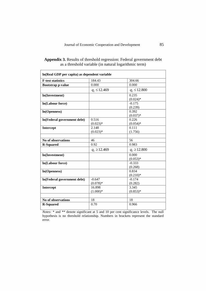
Journal of Economic Cooperation and Development 85
Appendix 3. Results of threshold regression: Federal government debt
as a threshold variable (in natural logarithmic term)
ln(Real GDP per capita) as dependent variable
F-test statistics 184.43 304.66
Bootstrap p-value 0.000 0.000
469.12iq 800.12iq
ln(Investment) 0.235
(0.024)*
ln(Labour force) -0.175
(0.239)
ln(Openness) 0.392
(0.037)*
ln(Federal government debt) 0.516
(0.023)*
0.226
(0.054)*
Intercept 2.148
(0.023)*
0.111
(1.756)
No of observations 46 56
R-Squared 0.92 0.983
469.12iq 800.12iq
ln(Investment) 0.000
(0.053)*
ln(Labour force) -0.333
(0.268)
ln(Openness) 0.834
(0.210)*
ln(Federal government debt) -0.647
(0.078)*
-0.174
(0.282)
Intercept 16.898
(1.000)*
3.345
(0.853)*
No of observations 18 18
R-Squared 0.70 0.966
Notes: * and ** denote significant at 5 and 10 per cent significance levels. The null
hypothesis is no threshold relationship. Numbers in brackets represent the standard
error.

86 The Real Effect of Government Debt:
Evidence from the Malaysian Economy
Appendix 4. Breitung (2001) non-linear cointegration test
Real GDP per capita as
dependent variable
Investment as dependent
variable
Rank test 0.020* 0.019*
Score test 7.495* 1.240
Notes: * and ** denote significant at 5 and 10 per cent significance levels. Critical
values for the rank test statistics are from Breitung (2001) and the null hypothesis of no
non-linear cointegration is rejected for a test statistic value smaller than the critical
value.
Appendix 5: List of variables
Variables Descriptions Sources
Real GDP per capita Real Gross Domestic product
per capita (2000 constant
prices)
Monthly Bulletin, Central
Bank of Malaysia
Investment Gross fixed capital formation
(in RM Million)
Monthly Bulletin, Central
Bank of Malaysia
Labour force Total labour force International Monetary
Fund/International Financial
Statistics
Openness Trade openness (exports plus
imports)
Monthly Bulletin, Central
Bank of Malaysia
XX Exports of goods and
services
Monthly Bulletin, Central
Bank of Malaysia
MM Imports of goods and
services
Monthly Bulletin, Central
Bank of Malaysia
Federal government
debt
Total Federal Government
external debt (in RM
Million)
Monthly Bulletin, Central
Bank of Malaysia
Fiscal surplus/ deficit (in RM Million) Monthly Bulletin, Central
Bank of Malaysia
Journal of Economic Cooperation and Development, 37, 3 (2016), 87-108
Environmental Kuznets Curve for Deforestation in Indonesia:
An ARDL Bounds Testing Approach
Efendi Agus Waluyo1 and Taku Terawaki
2
The main objective of this study is to empirically demonstrate the inverse
U-shaped relationship, which is generally called the environmental Kuznets
curve (EKC), between economic development and deforestation rate in
Indonesia. For this purpose, we analyzed time-series data for Indonesia over 46
years from 1962 to 2007 with the autoregressive distributed lag (ARDL)
bounds testing approach to cointegration. Results support the long-run
inverted-U relationship, which implies that, while the deforestation rate
increases at the initial stage of economic growth, it declines after a threshold
point. The income turning point of the EKC was calculated to be US$ 990.4.
These findings derived solely from the time-series data for Indonesia provide
helpful information for the Indonesian government and policy-makers in the
sense that it explicitly indicates the specific tendency for that country.
1. Introduction
A “grow first, clean up later” approach, which means that only the
economic growth is targeted with little regard for its environmental
impact, is the basic strategy that have been taken by many developing
countries. Unfortunately, the rapid economic growth in this strategy has
often caused unprecedented environmental degradation in an early stage
of the growth especially. Tropical deforestation is one of the examples.
Since the forestry sector is a major contributor to the economy in the
developing countries most part of whose land is covered in forest, the
initial economic growth in those countries have naturally a direct and
negative impact on the forest ecosystem. Flood damage occurring in all
parts of the world will be one piece of clear evidence showing the fact.
There is no doubt that it is one of the greatest concerns of many
1 Forestry Research Institute, Forestry Research and Development Agency (FORDA),
The Ministry of Forestry Republic of Indonesia E-mail address: [email protected] 2 College of Economics, Ritsumeikan University, Japan
88 Environmental Kuznets Curve for Deforestation in Indonesia:
An ARDL Bounds Testing Approach
developing countries to know whether “grow first, clean up later” is a
costly strategy in a long-run view, and whether it can be a threat against
the sustainability of growth itself.
Indonesia, which has the most extensive forest area in the ASEAN
nations, has also suffered from massive and rapid destruction of the
forests for the last few decades, while the country has experienced the
economic growth acceleration by extracting natural resources in its
“grow first, clean up later” strategy. The Food and Agriculture
Organization of the United Nations (FAO) shows that about 30 % of the
forest cover area in Indonesia had been lost during the period 1962-2007,
although the GDP per capita had increased by five times and more
during the same time. However, such a negative correlation between
these two economic and environmental indicators is not always applied.
The inverse U-shaped relationship between them, which is generally
called “environmental Kuznets curve (EKC)”, is a key concept in
understanding the impact of economic growth on deforestation. The
evidence of the existence of EKC for deforestation would encourage
developing countries facing the problem of serious forest loss to
advance their economic development.
The main objective of this study is to empirically demonstrate the
inverse U-shaped relationship between economic development and
deforestation rate in Indonesia. We also figure out the turning point at
which the increase in income level does not lead to the increase in
deforestation rate. For these purposes, time-series data for Indonesia
over 46 years from 1962 to 2007 was analyzed with the autoregressive
distributed lag (ARDL) bounds testing approach to cointegration,
developed by Pesaran and Shin (1998) recently. Although many relevant
previous studies have so far tested the EKC hypothesis for deforestation
with cross-country or panel data (Shafik and Bandyopadhyay, 1992;
Koop and Tole, 1999; Bhattarai and Hammig, 2001; Culas, 2007), to our
knowledge, no study exists as yet that has shown the existence of the
EKC on deforestation by using the data for a single country. The
findings derived solely from the time-series data for Indonesia would
provide helpful information for the Indonesian government and
policy-makers in the sense that it explicitly indicates the specific
tendency for that country.

Journal of Economic Cooperation and Development 89
The paper consists of six sections. Following this introduction, the
second section provides the literature review on previous EKC studies.
The third section explains the empirical model specified in this study
and the data employed for the analysis. The ARDL bounds testing
procedure will be described in the forth section. The fifth section
discusses the results and discussion. The key findings are summarized in
the sixth section, and then we conclude this paper with further
discussion.
2. Literature review on the EKC
The environmental Kuznets curve is a theoretical concept that describes
the relationship between income growth and environmental degradation.
The term is named for Simon Kuznets (1955) who proposed that a
connection between economic growth and income equality is shaped as
an inverted U. This inverted U-shape hypothesis for environmental
indicators were first examined by Grossman and Krueger (1991). They
found in their study that the concentrations of two air pollutants out of
three (sulfur dioxide and “smoke”) increases at a low level of national
income and decreases at a higher level of income by analyzing the data
for 42 countries. Studies on the EKC following Grossman and Krueger
(1991) have exhibited an inconsistent tendency. Panayotou (1995) and
Song et al. (2008) showed that the EKC hypothesis was supported for all
the pollutants employed in those studies in common, while Grossman
and Krueger (1995), Akbostanchi et al. (2009), Shaw et al. (2010)
demonstrated that the inverted U is not necessarily described for all the
environmental indicators. More recently, it is reported that the inverse
U-shaped relationship regarding carbon dioxide was accepted for China
(Jalil and Mahmud, 2009; Jalil and Feridun, 2011) and for France (Iwata
et al., 2010), but it was rejected for Turkey (Akbostanchi et al., 2009;
Ozturk and Acaravci, 2010) and for Russia (Pao et al., 2011). We also
have to note that these inconsistent results could be caused by the other
factors, such as model specification and employed variables (Stern,
2004).
The EKC studies regarding deforestation have also produced various
findings. In the two pioneering papers, mixed results are reported.
Shafik and Bandyopadhyay (1992) failed to explain the EKC

90 Environmental Kuznets Curve for Deforestation in Indonesia:
An ARDL Bounds Testing Approach
relationship between income and two types of deforestation indicators
(annual deforestation and total deforestation). In Panayotou (1995)1, on
the contrary, an inverse U-shaped relationship appeared to hold between
forest area and GDP per capita from the cross-sectional data covering 68
countries. The income turning point was estimated to be about US$ 800
in his research. Several studies that investigated the existence of the
EKC for each continent also do not show regular patterns. While
Bhattarai and Hammig (2001) suggested that there was a strong
evidence of the EKC relationship between income and deforestation for
all the three continents of Latin America, Africa, and Asia, Cropper &
Griffiths (1994) indicated that the EKC hypothesis was supported for
Latin America and Africa, but not for Asia. In the more recent research
by Culas (2007), the inverted-U shape was statistically accepted only for
Latin America. The existence of the EKC for Africa or Asia did not
result in being significant in that study. In addition, Koop and Tole
(1999) were unable to reject the hypothesis that the country-specific
coefficients of GDP and GDP squared were vary across the countries for
each of Latin America, Africa, and Asia. This implies the necessity of
estimating an individual EKC with the data for each single country, as
well as the difficulty of obtaining a single EKC relationship among all
the countries in a region.
3. Model specification and data
This study estimates the deforestation equation that describes the factors
affecting deforestation in Indonesia, by using time-series data for that
country over 46 years from 1962 to 2007. The empirical model is
specified as
(1) 𝐷𝐸𝐹 = 𝛼 + 𝛽1𝐺𝐷𝑃𝑡 + 𝛽2(𝐺𝐷𝑃𝑡)2 + 𝛽3𝑃𝑂𝑃𝐺𝑅𝑊𝑡
+ 𝛽4𝑅𝑃𝑂𝑃𝑡 + 𝛽5𝐴𝐺𝐼𝑡 + 𝛽6𝐴𝐺𝐿𝑡 + 𝛽7𝑅𝑊𝑂𝑂𝐷𝑡
+ 𝛽8𝐹𝑂𝑅𝐸𝑋𝑃𝑡 + 𝑢𝑡 ,
where DEF is the annual rate of deforestation, GDP is gross domestic
product per capita, POPGRW is population growth, RPOP is rural
population, AGI is agricultural index, AGL is agricultural land area,
RWOOD is roundwood production, FOREXP is forest products export,
1 The original paper was published in 1993 (Panayotou, 1993).

Journal of Economic Cooperation and Development 91
and ut is a stochastic error term. The subscript t refers to year t. The DEF,
which is the dependent variable in equation (1), is calculated as
(2) DEF = (Ft-1 – Ft) / Ft-1
where F is forest cover area. The data on forest cover area comes from
FAOSTAT released by FAO. For the GDP, which is the most important
data in the explanatory variables, we employ the real GDP per capita
converted into US dollars that is obtained from World Bank. The EKC
hypothesis for deforestation in Indonesia would be accepted, when the
coefficient of GDP is positive and the coefficient of GDP2 is negative in
equation (1).
As carried out by many previous EKC studies on deforestation, we also
include variables other than income as explanatory variables, because
the causes of deforestation are considered to be complex and interlinked.
In our analysis, the significances of population, agricultural, and forestry
factors, as well as income, are inspected. First, the variables of
population growth (POPGRW) and rural population (RPOP) are
included in the model to examine the impact of population pressure on
deforestation. Those variables have been widely used in previous
empirical studies (Cropper and Griffiths, 1994; Bhattari and Hammig,
2001; Barbier and Burgess, 2001; Culas, 2007). We obtained the data on
population growth from World Bank, and the data on rural population
from FAOSTAT. Population pressure can increase the demand for forest
products or alternative land uses that causes deforestation, but it might
also work so as to reduce the deforestation, inducing technological
progress or institutional changes in agricultural or forestry sector (Culas,
2007). Second, we add the variables of agricultural land area (AGL) and
agricultural production index2 (AGI) to the list of explanatory variables.
The purpose of adding them is to illustrate how the deforestation in
Indonesia is connected with the increase in agricultural production. The
two major strategies to promote agricultural production are the
expansion of agricultural land into forests and technological
improvement in agriculture. The AGL and AGI are employed as proxy
variables for them, respectively. Third, the model comprises roundwood
2 This index shows the relative level of the aggregate volume of agricultural
production for each year in comparison with that of the base period of 1999-2001.
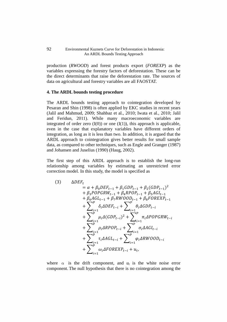
92 Environmental Kuznets Curve for Deforestation in Indonesia:
An ARDL Bounds Testing Approach
production (RWOOD) and forest products export (FOREXP) as the
variables expressing the forestry factors of deforestation. These can be
the direct determinants that raise the deforestation rate. The sources of
data on agricultural and forestry variables are all FAOSTAT.
4. The ARDL bounds testing procedure
The ARDL bounds testing approach to cointegration developed by
Pesaran and Shin (1998) is often applied by EKC studies in recent years
(Jalil and Mahmud, 2009; Shahbaz et al., 2010; Iwata et al., 2010; Jalil
and Feridun, 2011). While many macroeconomic variables are
integrated of order zero (I(0)) or one (I(1)), this approach is applicable,
even in the case that explanatory variables have different orders of
integration, as long as it is less than two. In addition, it is argued that the
ARDL approach to cointegration gives better results for small sample
data, as compared to other techniques, such as Engle and Granger (1987)
and Johansen and Juselius (1990) (Haug, 2002).
The first step of this ARDL approach is to establish the long-run
relationship among variables by estimating an unrestricted error
correction model. In this study, the model is specified as
(3) ∆𝐷𝐸𝐹𝑡
= 𝛼 + 𝛽0𝐷𝐸𝐹𝑡−1 + 𝛽1𝐺𝐷𝑃𝑡−1 + 𝛽2(𝐺𝐷𝑃𝑡−1)2
+ 𝛽3𝑃𝑂𝑃𝐺𝑅𝑊𝑡−1 + 𝛽4𝑅𝑃𝑂𝑃𝑡−1 + 𝛽5𝐴𝐺𝐼𝑡−1
+ 𝛽6𝐴𝐺𝐿𝑡−1 + 𝛽7𝑅𝑊𝑂𝑂𝐷𝑡−1 + 𝛽8𝐹𝑂𝑅𝐸𝑋𝑃𝑡−1
+ ∑ 𝛿𝑖𝛥𝐷𝐸𝐹𝑡−𝑖
𝑝
𝑖=1+ ∑ 𝜃𝑖𝛥𝐺𝐷𝑃𝑡−𝑖
𝑝
𝑖=1
+ ∑ 𝜇𝑖𝛥(𝐺𝐷𝑃𝑡−𝑖)2
𝑝
𝑖=1+ ∑ 𝜋𝑖𝛥𝑃𝑂𝑃𝐺𝑅𝑊𝑡−𝑖
𝑝
𝑖=1
+ ∑ 𝜌𝑖𝛥𝑅𝑃𝑂𝑃𝑡−𝑖
𝑝
𝑖=1+ ∑ 𝜎𝑖𝛥𝐴𝐺𝐼𝑡−𝑖
𝑝
𝑖=1
+ ∑ 𝜏𝑖𝛥𝐴𝐺𝐿𝑡−𝑖
𝑝
𝑖=1+ ∑ 𝜑𝑖𝛥𝑅𝑊𝑂𝑂𝐷𝑡−𝑖
𝑝
𝑖=1
+ ∑ 𝜔𝑖𝛥𝐹𝑂𝑅𝐸𝑋𝑃𝑡−𝑖
𝑝
𝑖=1+ 𝑢𝑡,
where α is the drift component, and ut is the white noise error
component. The null hypothesis that there is no cointegration among the

Journal of Economic Cooperation and Development 93
variables is expressed as β0=β1=β2=β3=β4=β5=β6=β7=β8.
We can conclude that there is a cointegration relationship among them,
if the calculated F-statistics is more than the upper critical bound given
by Pesaran et al., (2001). If the F-statistics is lower than the lower
critical bound, then it is judged that there is no cointegration. The
decision regarding cointegration will be inconclusive, when the
F-statistic lies within the upper and lower critical bounds.
Once a cointegration relationship among the variables is established, the
next step is to obtain the long-run equilibrium equation for deforestation
and its determinants. We can derive the reduced-form solution from
equation (3) as
(4) 𝐷𝐸𝐹𝑡 = 𝜆0 + 𝜆1𝐺𝐷𝑃𝑡 + 𝜆2(𝐺𝐷𝑃𝑡)2 + 𝜆3𝑃𝑂𝑃𝐺𝑅𝑊𝑡
+ 𝜆4𝑅𝑃𝑂𝑃𝑡 + 𝜆5𝐴𝐺𝐼𝑡 + 𝜆6𝐴𝐺𝐿𝑡 + 𝜆7𝑅𝑊𝑂𝑂𝐷𝑡
+ 𝜆8𝐹𝑂𝑅𝐸𝑋𝑃𝑡 + 𝑢𝑡 ,
where 𝜆0 = − 𝛼 𝛽0⁄ , 𝜆1 = − 𝛽1 𝛽0⁄ , 𝜆2 = − 𝛽2 𝛽0⁄ , 𝜆3 = − 𝛽3 𝛽0⁄ ,
𝜆4 = − 𝛽4 𝛽0⁄ , 𝜆5 = − 𝛽5 𝛽0⁄ , 𝜆6 = − 𝛽6 𝛽0⁄ , 𝜆7 = − 𝛽7 𝛽0⁄ , and
𝜆8 = − 𝛽8 𝛽0⁄ . On the other hand, the short-run dynamics is described in
the form of an error correction model (ECM) as
(5) ∆𝐷𝐸𝐹𝑡
= ∑ 𝛿𝑖𝛥𝐷𝐸𝐹𝑡−𝑖
𝑝
𝑖=1+ ∑ 𝜃𝑖𝛥𝐺𝐷𝑃𝑡−𝑖
𝑝
𝑖=1
+ ∑ 𝜇𝑖𝛥(𝐺𝐷𝑃𝑡−𝑖)2
𝑝
𝑖=1+ ∑ 𝜋𝑖𝛥𝑃𝑂𝑃𝐺𝑅𝑊𝑡−𝑖
𝑝
𝑖=1
+ ∑ 𝜌𝑖𝛥𝑅𝑃𝑂𝑃𝑡−𝑖
𝑝
𝑖=1+ ∑ 𝜎𝑖𝛥𝐴𝐺𝐼𝑡−𝑖
𝑝
𝑖=1
+ ∑ 𝜏𝑖𝛥𝐴𝐺𝐿𝑡−𝑖
𝑝
𝑖=1+ ∑ 𝜑𝑖𝛥𝑅𝑊𝑂𝑂𝐷𝑡−𝑖
𝑝
𝑖=1
+ ∑ 𝜔𝑖𝛥𝐹𝑂𝑅𝐸𝑋𝑃𝑡−𝑖
𝑝
𝑖=1+ ψ 𝐸𝐶𝑇𝑡−1 + 𝑢𝑡 ,
where the ECT is an error correction term.
To evaluate the goodness of fit of the model, we use several criteria.
These include classical assumption test, R-squared and adjusted

94 Environmental Kuznets Curve for Deforestation in Indonesia:
An ARDL Bounds Testing Approach
R-squared, lowest standard error of regression, lowest AIC, lowest SIC,
and model stability test. The technique employed to test model stability
is cumulative sum (CUSUM) and cumulative sum of squares
(CUSUMSQ). If the plots of CUSUM and CUSUMSQ statistics stay
within the critical bounds of 5 % level of significance, the null
hypothesis that all of the coefficients in the given regression are stable
cannot be rejected.
5. Results and discussion
5.1. Preliminary Examination
This study performs the conventional Augmented Dicky Fuller (ADF)
test and the Philip-Perron (PP) test to ensure that none of the variables
are I(2) or beyond. Table 1 shows the results of these unit root tests for
each variable. In the ADF test, the Swarchz Baysian Criterion (SBC)
was used to determine the optimal lag length. As shown in Table 1, the
results of ADF tests indicate that most of the variables are non-stationary
and have a unit root, while only the population growth (POPGRW) and
rural population (RPOP) are stationary at level. The results of PP tests
are also consistent with those of ADF tests. We can conclude from these
results that there is only a mixture of I(0) and I(1) among underlying
regressors. Hence, the ARDL bounds testing approach to cointegration
can be applied in this analysis (Duasa, 2007).
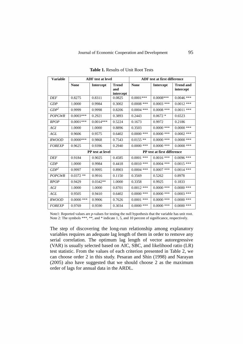
Journal of Economic Cooperation and Development 95
Table 1. Results of Unit Root Tests
Variable ADF test at level ADF test at first difference
None Intercept Trend
and
intercept
None Intercept Trend and
intercept
DEF 0.8275 0.8311 0.0825 0.0001*** 0.0008*** 0.0046 ***
GDP 1.0000 0.9984 0.3002 0.0008 *** 0.0003 *** 0.0012 ***
GDP2 0.9999 0.9998 0.8206 0.0004 *** 0.0008 *** 0.0011 ***
POPGWR 0.0003*** 0.2921 0.3893 0.2443 0.0672 * 0.6523
RPOP 0.0001*** 0.0014*** 0.5224 0.1673 0.9972 0.2186
AGI 1.0000 1.0000 0.8896 0.3503 0.0000 *** 0.0000 ***
AGL 0.9606 0.9575 0.6402 0.0000 *** 0.0000 *** 0.0002 ***
RWOOD 0.0000*** 0.9868 0.7543 0.0155 ** 0.0000 *** 0.0000 ***
FOREXP 0.9625 0.9396 0.2940 0.0000 *** 0.0000 *** 0.0000 ***
PP test at level PP test at first difference
DEF 0.9184 0.9025 0.4585 0.0001 *** 0.0016 *** 0.0096 ***
GDP 1.0000 0.9984 0.4418 0.0010 *** 0.0004 *** 0.0015 ***
GDP2 0.9997 0.9995 0.8903 0.0004 *** 0.0007 *** 0.0014 ***
POPGWR 0.0372 ** 0.9916 0.1150 0.3569 0.5262 0.8978
RPOP 0.9429 0.0342** 1.0000 0.3358 0.9925 0.1833
AGI 1.0000 1.0000 0.8701 0.0012 *** 0.0000 *** 0.0000 ***
AGL 0.9505 0.9410 0.6402 0.0000 *** 0.0000 *** 0.0003 ***
RWOOD 0.0000 *** 0.9906 0.7626 0.0001 *** 0.0000 *** 0.0000 ***
FOREXP 0.9769 0.9590 0.3034 0.0000 *** 0.0000 *** 0.0000 ***
Note1: Reported values are p-values for testing the null hypothesis that the variable has unit root.
Note 2: The symbols ***, **, and * indicate 1, 5, and 10 percent of significance, respectively.
The step of discovering the long-run relationship among explanatory
variables requires an adequate lag length of them in order to remove any
serial correlation. The optimum lag length of vector autoregressive
(VAR) is usually selected based on AIC, SBC, and likelihood ratio (LR)
test statistic. From the values of each criterion presented in Table 2, we
can choose order 2 in this study. Pesaran and Shin (1998) and Narayan
(2005) also have suggested that we should choose 2 as the maximum
order of lags for annual data in the ARDL.
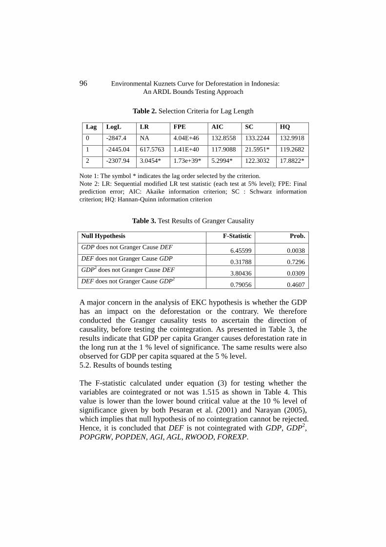
96 Environmental Kuznets Curve for Deforestation in Indonesia:
An ARDL Bounds Testing Approach
Table 2. Selection Criteria for Lag Length
Lag LogL LR FPE AIC SC HQ
0 -2847.4 NA 4.04E+46 132.8558 133.2244 132.9918
1 -2445.04 617.5763 1.41E+40 117.9088 21.5951* 119.2682
2 -2307.94 3.0454* 1.73e+39* 5.2994* 122.3032 17.8822*
Note 1: The symbol * indicates the lag order selected by the criterion.
Note 2: LR: Sequential modified LR test statistic (each test at 5% level); FPE: Final
prediction error; AIC: Akaike information criterion; SC : Schwarz information
criterion; HQ: Hannan-Quinn information criterion
Table 3. Test Results of Granger Causality
Null Hypothesis F-Statistic Prob.
GDP does not Granger Cause DEF 6.45599 0.0038
DEF does not Granger Cause GDP 0.31788 0.7296
GDP2 does not Granger Cause DEF
3.80436 0.0309
DEF does not Granger Cause GDP2
0.79056 0.4607
A major concern in the analysis of EKC hypothesis is whether the GDP
has an impact on the deforestation or the contrary. We therefore
conducted the Granger causality tests to ascertain the direction of
causality, before testing the cointegration. As presented in Table 3, the
results indicate that GDP per capita Granger causes deforestation rate in
the long run at the 1 % level of significance. The same results were also
observed for GDP per capita squared at the 5 % level.
5.2. Results of bounds testing
The F-statistic calculated under equation (3) for testing whether the
variables are cointegrated or not was 1.515 as shown in Table 4. This
value is lower than the lower bound critical value at the 10 % level of
significance given by both Pesaran et al. (2001) and Narayan (2005),
which implies that null hypothesis of no cointegration cannot be rejected.
Hence, it is concluded that DEF is not cointegrated with GDP, GDP2,
POPGRW, POPDEN, AGI, AGL, RWOOD, FOREXP.

Journal of Economic Cooperation and Development 97
Table 4. Result of Cointegration Test (including all the variables)
Equation DEF = f (GDP, GDP2, POPGRW, RPOP, AGI, AGL, RWOOD, FOREXP)
Lag structure ARDL (2,2,2,2,2,2,2,2,2)
F-statistic 1.515425
Significance
level
Bound critical values of Case III (Unrestricted intercept and no trend)
Pesaran et al. (2001) Narayan (2005)
I(0) I(1) I(0) I(1)
1% 3.41 4.68 4.030 5.598
5% 2.62 3.79 2.922 4.268
10% 2.26 3.35 2.458 3.647
Since no evidence of cointegration was detected among all the variables,
we next attempted to narrow the variables down.We finally selected the
variables of RPOP, AGI, and RWOOD, as well as GDP and GDP2,
based on the statistical significance of those variables. The F-statistic
calculated again (=3.564) was higher than the upper bound critical value
provided by Pesaran et al. (2001) at the 10 % level of significance. This
implies that the null hypothesis of no cointegration can be rejected at the
10 % level, but it has not been supported yet according to the Narayan’s
critical values.
Then, we eliminated insignificant variables, except for the level
variables and the intercept, with the general-to-specific approach
(Krolzig and Hendry, 2001). The results are displayed in Table 5. The
F-statistic (=4.183) is higher than the upper critical value at the 5 %
level of significance given by Pesaran et al. (2001), and at the 10 %
level by Narayan (2005). It suggests that the variables are cointegrated,
and confirms the existence of long-run relationship among them.
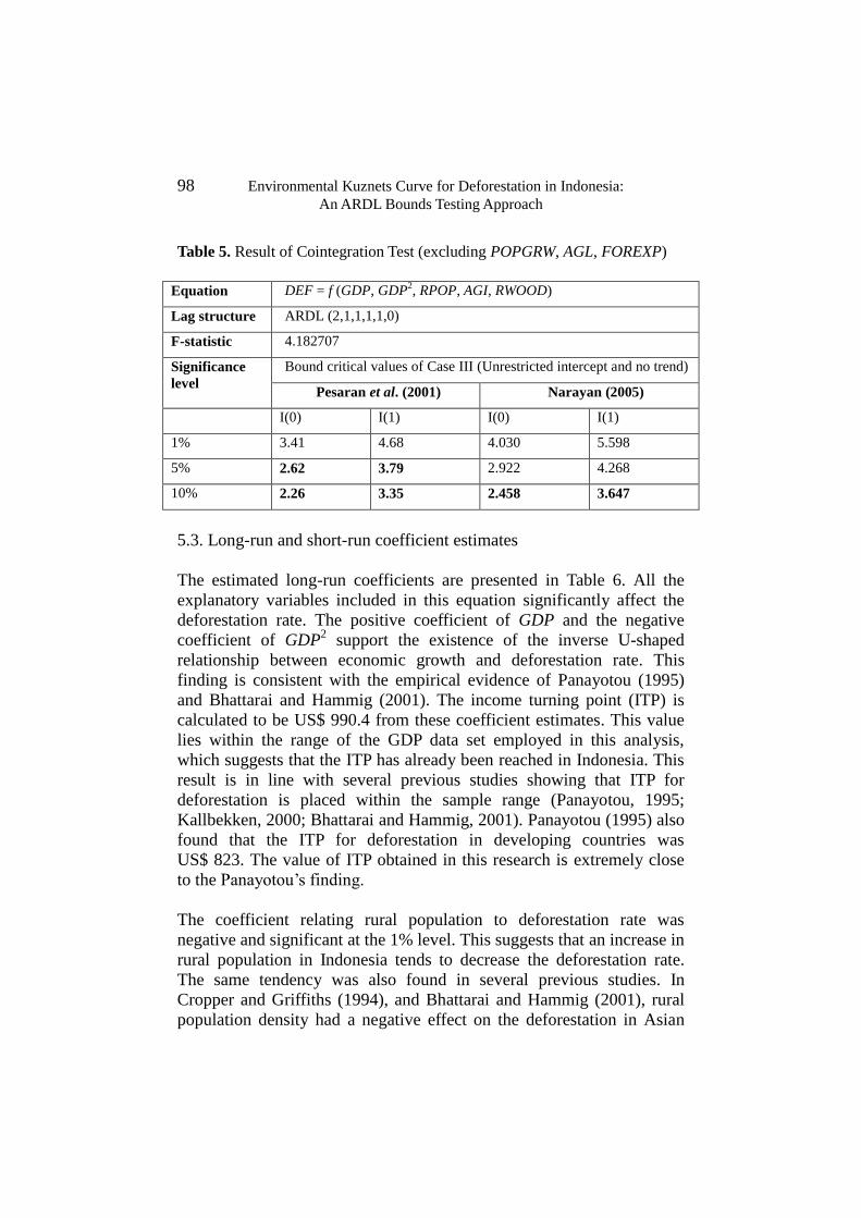
98 Environmental Kuznets Curve for Deforestation in Indonesia:
An ARDL Bounds Testing Approach
Table 5. Result of Cointegration Test (excluding POPGRW, AGL, FOREXP)
Equation DEF = f (GDP, GDP2, RPOP, AGI, RWOOD)
Lag structure ARDL (2,1,1,1,1,0)
F-statistic 4.182707
Significance
level
Bound critical values of Case III (Unrestricted intercept and no trend)
Pesaran et al. (2001) Narayan (2005)
I(0) I(1) I(0) I(1)
1% 3.41 4.68 4.030 5.598
5% 2.62 3.79 2.922 4.268
10% 2.26 3.35 2.458 3.647
5.3. Long-run and short-run coefficient estimates
The estimated long-run coefficients are presented in Table 6. All the
explanatory variables included in this equation significantly affect the
deforestation rate. The positive coefficient of GDP and the negative
coefficient of GDP2 support the existence of the inverse U-shaped
relationship between economic growth and deforestation rate. This
finding is consistent with the empirical evidence of Panayotou (1995)
and Bhattarai and Hammig (2001). The income turning point (ITP) is
calculated to be US$ 990.4 from these coefficient estimates. This value
lies within the range of the GDP data set employed in this analysis,
which suggests that the ITP has already been reached in Indonesia. This
result is in line with several previous studies showing that ITP for
deforestation is placed within the sample range (Panayotou, 1995;
Kallbekken, 2000; Bhattarai and Hammig, 2001). Panayotou (1995) also
found that the ITP for deforestation in developing countries was
US$ 823. The value of ITP obtained in this research is extremely close
to the Panayotou’s finding.
The coefficient relating rural population to deforestation rate was
negative and significant at the 1% level. This suggests that an increase in
rural population in Indonesia tends to decrease the deforestation rate.
The same tendency was also found in several previous studies. In
Cropper and Griffiths (1994), and Bhattarai and Hammig (2001), rural
population density had a negative effect on the deforestation in Asian

Journal of Economic Cooperation and Development 99
region. In addition, Reis and Guzman (1994) obtained the negative sign
of the coefficient of rural population in the case of Amazon deforestation.
Culas (2007) also detected a negative coefficient of population density.
Templeton and Scherr (1999) noted that population pressure on forest
resources will increase at first, but it will change along with efficiency in
production processes into the direction of the conservation of the
remaining forest resources. This result might be related to the
technological or institutional innovation induced from population
pressure.
As to the agricultural indicators, the AGI significantly affects the
deforestation rate in a negative way. This implies that an increase in
agricultural production does not promote the conversion of forest lands
to agricultural lands, and that the increase has been led by improving
technology in agriculture. Technological progress in agriculture must
reduce the pressure on land demand and slow down the speed of
deforestation.
Roundwood production was also significantly connected to the
deforestation rate in Indonesia. This negative coefficient of RWOOD
indicates that the deforestation rate decreases with increasing log
production. Allen and Barnes (1985) that examined the effect of wood
use on forest area change over 1968-78 in developing countries, also
found a negative coefficient of wood use variable. This result may be
closely associated with that the data on roundwood production used in
this study is legally reported one. The roundwood products reported
legally are probably the ones that come from the forest managed
sustainably, and thus they cannot be a cause of deforestation.
Unfortunately, many log products have not been officially reported and
some of them are illegally produced. There is also evidence that large
amounts of timber traded in the world market are harvested illegally
(Hembery et al., 2007). The increase in illegal logs may decrease the
production of legal logs, and may cause higher deforestation at the same
time.
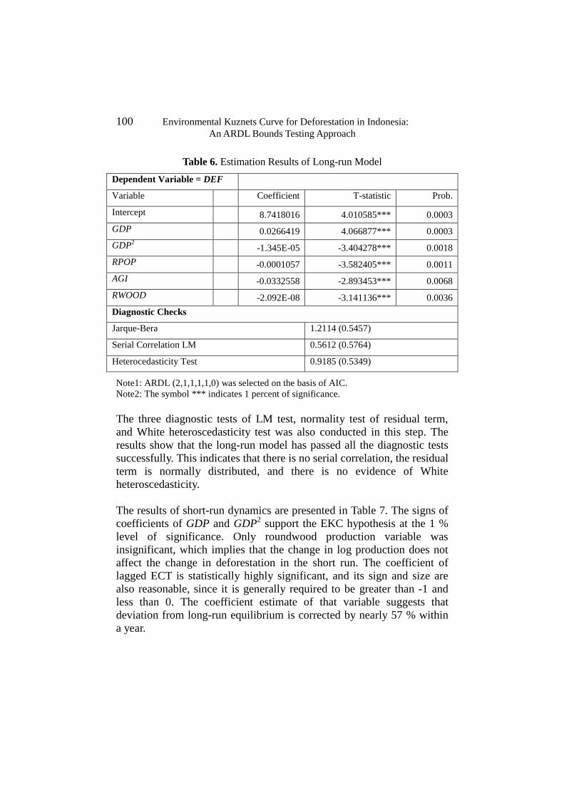
100 Environmental Kuznets Curve for Deforestation in Indonesia:
An ARDL Bounds Testing Approach
Table 6. Estimation Results of Long-run Model
Dependent Variable = DEF
Variable Coefficient T-statistic Prob.
Intercept 8.7418016 4.010585*** 0.0003
GDP 0.0266419 4.066877*** 0.0003
GDP2 -1.345E-05 -3.404278*** 0.0018
RPOP -0.0001057 -3.582405*** 0.0011
AGI -0.0332558 -2.893453*** 0.0068
RWOOD -2.092E-08 -3.141136*** 0.0036
Diagnostic Checks
Jarque-Bera 1.2114 (0.5457)
Serial Correlation LM 0.5612 (0.5764)
Heterocedasticity Test 0.9185 (0.5349)
Note1: ARDL (2,1,1,1,1,0) was selected on the basis of AIC.
Note2: The symbol *** indicates 1 percent of significance.
The three diagnostic tests of LM test, normality test of residual term,
and White heteroscedasticity test was also conducted in this step. The
results show that the long-run model has passed all the diagnostic tests
successfully. This indicates that there is no serial correlation, the residual
term is normally distributed, and there is no evidence of White
heteroscedasticity.
The results of short-run dynamics are presented in Table 7. The signs of
coefficients of GDP and GDP2 support the EKC hypothesis at the 1 %
level of significance. Only roundwood production variable was
insignificant, which implies that the change in log production does not
affect the change in deforestation in the short run. The coefficient of
lagged ECT is statistically highly significant, and its sign and size are
also reasonable, since it is generally required to be greater than -1 and
less than 0. The coefficient estimate of that variable suggests that
deviation from long-run equilibrium is corrected by nearly 57 % within
a year.

Journal of Economic Cooperation and Development 101
Table 7. Estimation Results of Short-run Model
Dependent Variable = ΔDEF
Variable Coefficie
nt
T-statistic Prob.
Intercept 0.463402 4.046573*** 0.0002
ΔGDP 0.014194 3.554423*** 0.0010
ΔGDP2 -7.52E-06 -3.168890*** 0.0030
ΔRPOP 0.000505 5.236923*** 0.0000
ΔAGI -0.029510 -3.919570*** 0.0004
ECT(-1) -0.568800 -5.676490*** 0.0000
Diagnostic Checks
Jarque-Bera 0.8867 (0.6418)
Serial Correlation LM 0.7740 (0.4689)
Heterocedasticity test 0.9760 (0.4634)
Note1: ARDL (2,1,1,1,1,0) was selected on the basis of AIC.
Note2: The symbol *** indicates 1 percent of significance.
Note3: ECT = DEF - 0.0266419*GDP + 1.345E-05*GDP2 + 0.0001057*RPOP +
0.0332558*AGI + 2.092E-08*RWOOD - 8.7418016
The last stage of ARDL bounds testing approach is to check the stability
of parameter estimates included in the model. In order to test the
stability, cumulative sum (CUSUM) and cumulative sum of squares
(CUSUMSQ) tests are generally performed. Figure 1 exhibits the plots
of CUSUM and CUSUMSQ, respectively. We can see from this figure
that the statistics are well within the critical bounds, which means that
all the parameter estimates in the model are stable.
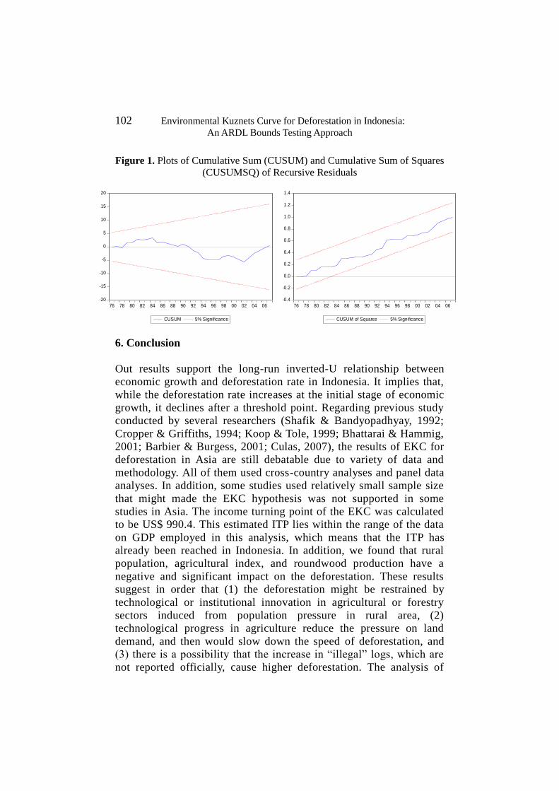
102 Environmental Kuznets Curve for Deforestation in Indonesia:
An ARDL Bounds Testing Approach
Figure 1. Plots of Cumulative Sum (CUSUM) and Cumulative Sum of Squares
(CUSUMSQ) of Recursive Residuals
6. Conclusion
Out results support the long-run inverted-U relationship between
economic growth and deforestation rate in Indonesia. It implies that,
while the deforestation rate increases at the initial stage of economic
growth, it declines after a threshold point. Regarding previous study
conducted by several researchers (Shafik & Bandyopadhyay, 1992;
Cropper & Griffiths, 1994; Koop & Tole, 1999; Bhattarai & Hammig,
2001; Barbier & Burgess, 2001; Culas, 2007), the results of EKC for
deforestation in Asia are still debatable due to variety of data and
methodology. All of them used cross-country analyses and panel data
analyses. In addition, some studies used relatively small sample size
that might made the EKC hypothesis was not supported in some
studies in Asia. The income turning point of the EKC was calculated
to be US$ 990.4. This estimated ITP lies within the range of the data
on GDP employed in this analysis, which means that the ITP has
already been reached in Indonesia. In addition, we found that rural
population, agricultural index, and roundwood production have a
negative and significant impact on the deforestation. These results
suggest in order that (1) the deforestation might be restrained by
technological or institutional innovation in agricultural or forestry
sectors induced from population pressure in rural area, (2)
technological progress in agriculture reduce the pressure on land
demand, and then would slow down the speed of deforestation, and
(3) there is a possibility that the increase in “illegal” logs, which are
not reported officially, cause higher deforestation. The analysis of
-20
-15
-10
-5
0
5
10
15
20
76 78 80 82 84 86 88 90 92 94 96 98 00 02 04 06
CUSUM 5% Significance
-0.4
-0.2
0.0
0.2
0.4
0.6
0.8
1.0
1.2
1.4
76 78 80 82 84 86 88 90 92 94 96 98 00 02 04 06
CUSUM of Squares 5% Significance
Journal of Economic Cooperation and Development 103
short-run dynamics also reveals that the deviation from the long-run
equilibrium is quickly adjusted.
While the EKC results obtained from cross-country information
clearly shows an inverse U-shaped relationship as a whole between
economic development and environmental degradation, they would be
insufficient for each developing country facing the issue of whether
the development of the country is sustainable or not to be
optimistically confident that “grow first, clean up later” strategy will
work well in that country. As described above, several previous
studies analyzing these data, in fact, have revealed that there exist
different EKCs among continents. In terms of practical policy-making
on sustainable development, it would be necessary to test the
existence of the specific EKC for each country. This study definitely
demonstrates the usefulness of adopting the ARDL approach in the
evaluation of EKC hypothesis for a single country.
Due to data restriction, it was not possible to use provincial data in
this study. Using provincial data would provide a more valuable
insight into policy making, because they can introduce the effect of
region to the model. Another weakness of this study is that there is no
policy variable in the empirical model. Policy variables that could be
included are, for example, international environmental agreement,
enforcement of environmental legislation, and green project policy
(e.g. forest and land rehabilitation movement). The addition of these
variables would facilitate explaining what kinds of policies can
reduce deforestation.

104 Environmental Kuznets Curve for Deforestation in Indonesia:
An ARDL Bounds Testing Approach
References
Akbostanci, E., Türüt-Asik, S., Tunc, G. I., 2009. The relationship
between income and environment in Turkey: Is there an environmental
Kuznets curve? Energy Policy, 37 (2), 861-867.
Allen, J.C., Barnes, D.F., 1985. The causes of deforestation in
developing countries. Annals of the Association of American
Geographers, 75 (2), 163-184.
Barbier, E.B., Burgess, J.C., 2001. The economics of tropical
deforestation. Journal of Economic Survey, 15 (3), 413-433.
Bhattarai, M., Hammig, M,. 2001. Institutions and the environmental
Kuznets Curve for deforestation: A cross-country analysis for Latin
America, Africa, and Asia. World Development, 29 (6), 995-1010.
Cropper, M., Griffits, C., 1994. The interaction of population growth and
environmental quality. The American Economic Review, 84 (2), 250-254.
Culas, R.J., 2007. Deforestation and the environmental Kuznets curve:
An institutional perspective. Ecological Economics, 61 (2-3), 429-437.
Duasa, J., 2007. Determinants of Malaysian trade balance: An ARDL
bound testing approach. Journal of Economic Cooperation, 28 (3),
21-50.
Engle, R. F., Granger, C. W. J., 1987. Cointegration and error correction
representation: estimation and testing. Econometrica, 55 (2), 251-276.
Grossman, G. M, Krueger, A. B., 1991. Environmental impacts of a
North American free trade agreement. NBER Working Paper 3914. MA:
National Bureau of Economic Research, Cambridge.
Grossman, G.M., Krueger, A.B., 1995. Economic growth and the
environment. Quarterly Journal of Economics, 110 (2), 353–377.
Journal of Economic Cooperation and Development 105
Haug, A.A., 2002. Temporal aggregation and the power of cointegration
test: A Monte Carlo study. Oxford Bulletin of Economics and Statistic,
64 (4), 399-412.
Hembery, R., Jenkins, A., White, G., Richards B., 2007. Illegal logging:
Cut it out! The UK’s role in the trade in illegal timber and wood product.
WWF UK Illegal logging report.
Iwata H., Okada, K., Samreth, S., 2010. Empirical study on the
environmental Kuznets curve for CO2 in France: The role of nuclear
energy. Energy Policy, 38 (8), 4057–4063.
Jalil, A., Mahmud, S.F., 2009. Environmental Kuznets curve for CO2
emissions: A cointegration analysis for China. Energy Policy, 37 (12),
5167-5172.
Jalil, A., Feridun, M., 2011. The impact of growth, energy and financial
development on the environment in China: A cointegration analysis.
Energy Economics, 33 (2), 284-291.
Johansen, S., Juselius, K., 1990. Maximum likelihood estimation and
inference on cointegration with applications to the demand for money.
Oxford Bulletin of Economics and Statistics, 52 (2), 169-210.
Kallbekken, S., 2000. An alternative environmental Kuznets curve
approach to deforestation. Disertation in Environmental Economics and
Environmental Management. University of York, UK.
Koop, G., Tole, L., 1999. Is the an environmental Kuznets Curve for
deforestation? Journal of Development Economics, 58 (1), 231-244.
Krolzig, H-M., Hendry, D.F., 2001. Computer automation of
general-to-specific model selection procedures. Journal of Economic
Dynamics and Control, 25 (6-7), 831-866.
Kuznets, S., 1955. Economic growth and income inequality. The
American Economic Review 45 (1), 1-28.

106 Environmental Kuznets Curve for Deforestation in Indonesia:
An ARDL Bounds Testing Approach
Narayan, P.K., 2005. The saving and investment nexus for China:
Evidence from cointegration tests. Applied Economics, 37 (17),
1979-1990.
Ozturk, I., Acaravci, A., 2010. CO2 emissions, energy consumption and
economic growth in Turkey. Renewable and Sustainable Energy Reviews,
14 (9), 3008-3014.
Panayotou, T., 1993. Empirical Tests and Policy Analysis of
Environmental Degradation at Different Stages of Economic
Development. Working Paper WP238: Technology and Employment
Programme, ILO.
Panayotou, T., 1995. Environmental degradation at different stages of
economic development. In: Ahmed, I. and J.A. Doeleman (Eds.),
Beyond Rio: The environmental crisis and sustainable livelihoods in the
third world. ILO, MacMillan Press Ltd., London, pp. 13-36.
Pao, H.-T., Yu, H.-C., Yang, Y.-H., 2011. Modelling the CO2 emissions,
energy use, and economic growth in Russia. Energy, 36 (8), 5094-5100.
Pesaran, M.H., Shin, Y., 1998. An autoregressive distributed lag
modeling approach to cointegration analysis. A revised version of a
paper presented at the Symposium at the Centennial of Ragnar Frisch,
The Norwegian Academy of Science and Letters, Oslo, March 3-5,
1995. In: Strom, S. (Eds.), Econometrics and Economic Theory in the
20th
Century. Cambridge University Press, UK, pp. 371-413.
Pesaran, M.H., Shin, Y., Smith, R.J., 2001. Bounds testing approaches to
analysis of level relationship. Journal of Applied Econometrics, 16 (3),
289-326.
Reis, E., Guzman, R., 1994. An econometric model of Amazon
deforestation. In: Brown, K., Pearce, D.W. (Eds.), The Causes of
Tropical Deforestation: The economic and statistical analysis of factors
giving rise to the loss of the tropical. UBC Press, Vancouver, Canada, pp.
172-191.

Journal of Economic Cooperation and Development 107
Shafik, N., Bandyopadhyay, S., 1992. Economic growth and
environmental quality: Time-series and cross-country evidence. Policy
Research Working Paper. World Development Report.
Shahbaz, M., Jamil, A., Dube, S., 2010. Environmental Kuznets curve
(EKC): Time series evidence from Portugal. MPRA Paper No.27443, 15
October.
Shaw, D., Pang, A., Lin, C-C., Hung., M-F., 2010. Economic growth and
air quality in China. Environmental Economics and Policy Studies, 12
(3), 179-196.
Song, T., Zheng, T., Tong, L., 2008. An empirical test of the
environmental Kuznets curve in China: A panel cointegration approach.
China Economic Review, 19 (3), 381-392.
Stern, D.I., 2004. The rise and fall of the environmental Kuznets curve.
World Development, 32 (8), 1419–1439.
Templeton, S.R., Scherr, S.J., 1999. Effect of demographic and related
microeconomic change on land quality in hills and mountains of
developing countries. World Development, 27 (6), 903-918.


Journal of Economic Cooperation and Development, 37, 3 (2016), 109-134
Determination of the Degree of Development and the Impact of the
Information Environment on the Formation of A System of Social
Control in Procurement Under the Russian Contract System (Method
of Content Analysis of Information Resources on the Internet)
N.A. Mamedova
1 and A.N. Baykova
2
The article is a result of research on the effect of environment on the
development of information system of social control in procurement.
Informatization process of social relations largely determines how certain
trends of social activity will be popular and durable. To determine the degree
of maturity of information content on the theme of social control in
procurement in Russia, the study used the method of content analysis of
information resources. To improve the quality of research results were
analyzed according to the semiotic and conceptual and thematic units of
content.
Introduction
Content analysis is a method of research aimed at quantitative analysis
of texts and text arrays for subsequent meaningful interpretation of
numerical patterns identified. The primary mechanism of the method is
the identification and measurement of the frequency of the use of formal
or substantive components were analyzed in total individual text or data
array. The degree of frequency of use in this sense becomes the desired
indicator. The method is used to visualize the dynamics of the intuitions
of the text content (information file) on a repetitive manner, estimates,
opinions and other forms of expression in order to be able to organize
these intuitive feelings, give them meaningful and reasoned explanation
of the subject. Using the method involves the development of targeted
approaches to the collection of data, representing the contextual textual
evidence on which the feeling of repetition and repetition frequency
based. However, the potential of the method of content analysis may be
1 Moscow State University of Economics, Statistics and Informatics (MESI), Moscow
Email: [email protected] (first author) 2 Moscow State University of Economics, Statistics and Informatics (MESI), Moscow
Email: [email protected]

110 Determination of the Degree of Development and the Impact of the
Information Environment on the Formation of a System of Social Control
in Procurement Under the Russian Contract System
(Method of Content Analysis of Information Resources on the Internet)
represented by a much wider. Using the method, the researcher can not
only streamline their understanding of the text (information files), but
also to justify their conclusions, to interpret the author's position on the
nature of used them formal elements or structures, revealing even more
than the author would like to put into words. In this regard, the content
analysis method called the "scientific method of reading between the
lines."
Thus, a systematic approach to the study of the context, the desire for
objectification of the data analysis of the text or information set is non-
exclusive characteristic of content analysis and observed with the use of
other methods of word processing. However, the establishment of
quality parameters of the text (information files) through a quantitative
measurement of the formal elements and establish the relation between
the detected quantitative indicators is a characteristic feature of content
analysis as a method of scientific knowledge in the methods of analysis
and processing of texts. Therefore, the need to clarify the definition of
the method. Content analysis is a systematic quantitative analysis,
evaluation and interpretation of the form and content of information
sources. This type of analysis is primarily quantitative analysis reveals
quantitative regularities of repetition components of text, while in the
analysis may reveal structural patterns, qualitative laws by classification,
ranking and establishing a causal relationship between the obtained
results of content analysis.
Over other methods of analysis and processing of text content analysis
method has several advantages. For example, advantage is its
adaptability, which manifests itself in the possibility of using the method
without limitation as to the minimum and the maximum volume of the
analyzed information. Processability method also evident in its effective
integration with many other methods, in relation to which the method of
content analysis, and can act as a primary, and as collateral. This method
is most suitable for the primary processing of large volumes of
information and adjusting the flow of information on the stage of
collecting and processing raw data for both theoretical and applied
research. Also indisputable advantage is the possibility of formalization
and computerization of the process and the results of the content
analysis, due to its characteristics as a quantitative method of analysis
and text processing.

Journal of Economic Cooperation and Development 111
Results and Discussion
As mentioned above, the mechanism of the method of content analysis
is to calculate the frequency of occurrence of certain components in the
analyzed text or data arrays, which is complemented by the
identification of qualitative relationships (statistical methods) and
structural relationships (through the analysis of structural relationships
between the components). The result of the method is considered to
justify the existence of some analytes in quantitative and qualitative
characteristics. Obviously, the effectiveness of the method is due to the
choice of components, i.e., the choice of units of analysis. Requirements
for the unity of content analysis are obvious enough. Firstly, it should be
easily identified in the text. Secondly, a unit of content analysis should
enable the semantic interpretation, that is to be interesting and useful
content in the scale of the study. The tasks of the content analysis
conducted for the purpose of the study were a content analysis on the
structural-semiotic units (keywords) and the conceptual and thematic
units. To conduct content analysis were used open sources of
information and communication on the Internet. To clarify the
parameters of the sampling information it was decided to use the data set
generated by the search engines. When choosing a search engine we
used the following criteria: a high degree of relevance of search results;
optimal set of advanced search functions; low percentage of references
to duplicate content; absence (very low percentage) relevance of links
aimed at commercial sites. With all of these criteria best search engine
was determined search system Google.
To conduct content analysis on the structural-semiotic units and specific
to the research conducted as keywords accepted words the phrase "social
control in procurement."
Public control of procurement is defined by the law mechanism for the
rights of citizens, public associations, associations of legal entities to
control the legitimacy of the state and municipal customers. At its core,
social control in procurement is a form of interaction between civil
society and the state to ensure the functioning of the legal order of the
contract system in the procurement of goods, works and services for
state and municipal needs. The objectives of social control in
procurement include: a full submission of information, the development
of civil society, reducing corruption, development of markets and trade

112 Determination of the Degree of Development and the Impact of the
Information Environment on the Formation of a System of Social Control
in Procurement Under the Russian Contract System
(Method of Content Analysis of Information Resources on the Internet)
relations. The implementation of these tasks is possible through the
creation of an open information space in which interactions (functional
level set), all participants of the contract system and society.
The legal basis for the functioning of social control in procurement in
Russia is so basic pieces of legislation: Federal Law № 112-FL "On the
basis of public control" and the Federal Law № 44-FL "On the contract
system in the procurement of goods, works and services for state and
municipal needs". Federal Law № 112-FL establishes the legal basis for
the organization and implementation of public control over the activities
of state authorities, local government, state and municipal organizations,
other agencies and organizations engaged in accordance with federal
laws separate public authority. In turn, the Federal Law № 44-FL
regulates relations directed at providing state and municipal needs in
order to improve efficiency, effectiveness of the procurement of goods,
works and services, ensure openness and transparency of such
purchases, the prevention of corruption and other abuses in the field of
procurement. And as one of the types of control procurement establishes
public oversight.
Thus, the legal framework of public control in procurement functions in
Russia, however, the activity of the subjects of public control is
insufficient. This study aims to assess the importance of social control in
procurement by analyzing the information field and placed it open
sources of information.
To evaluate the frequency of use of keywords in the information
resources, the results of extended context search were distributed in
accordance with the classification of information sources. In accordance
with the above keyword structural-semiotic research source was defined
thematic filter information resources (sites, portals). As classification
criterion, it was decided to use the theme filter in combination with the
degree of importance of the topic in the structure and content of web
pages, the totality of which was formed by the results of the extended
context search. Thus, information sources are classified as follows:
site (portal), specializing in the topic;
site (portal) wide profile information (main theme - procurement);

Journal of Economic Cooperation and Development 113
site (portal) independent profile - specialization relating missing
(news, panoramic, education);
site (portal) government or municipal authority;
site (portal) social organization, specializing on the subject of
procurement;
site (portal) social organization wide information profile;
site (portal) reference and the legal system;
links to educational materials, bills.
As the advanced search options in the search engine Google has taken
the following mandatory parameters (Table 1).
Advanced search options on the structural-semiotic units
Name of the parameter Basic / additional search
terms
The value of the selected
parameter
Select Keyword Keywords Public control procurement
Choice phrases Phrases Procurement for the needs
Search pages in the selected
language
Language web page In Russian
Search pages created in a
particular country
Country of creating web
pages
Russia
Search pages created or
updated within the
specified time
Date of creation / update Any
Search by text, title or
address of a page, as well
as links to them
Location words Anywhere on the page
Safe Search Blocking inappropriate
content
The function is activated
Search pages and files of a
certain format
File Format Either
Search for pages that are
free to use, distribute and
modify
Rights of use With any license

114 Determination of the Degree of Development and the Impact of the
Information Environment on the Formation of a System of Social Control
in Procurement Under the Russian Contract System
(Method of Content Analysis of Information Resources on the Internet)
Materials and methods
Content analysis on the structural-semiotic units.
To evaluate the results obtained by sampling information into account
results in a certain time interval. Thus, the search results were classified
according to the three stages of the legal regulation of the procurement
activities in the Russian Federation: the information resources available
and updated up to 2012; Information Resources posted and updated in
the period 2012-2013; Information Resources posted and updated in
2014. Thus, the search covers a period of №94 federal law, the
transitional period for the formation of the contract system (2012-2013)
and the period of commencement of the contract system, regulated by
federal law №44 (2014). The total number of information sources that
match the search parameters, the source is 133. This number is the result
of contextual search and does not include the hidden results (results are
homogeneous (similar) presented the results of the search context).
Besides the classification of search results for the sources of information
and limitation of accommodation (update) web page for evaluating
advanced context sensitive searches used the following methods of
ranking results on the basis of scoring. The first direction ranking -
ranking Compliance common sense content of Internet pages (text)
keywords, i.e. structural-semiotic unit conducted a content analysis. This
approach allows taking into account the ranking parameter randomness
use keywords. The second direction of ranking is ranking in order of
importance of keywords in the content of the web page (text). Ranging
in this direction allows considering setting the frequencies of keywords
on a page (text). The order of distribution of GMAT results extended
context of keyword search in accordance with a first direction of the
ranking (in the parameter randomness use keywords) is defined the
following:
If the text is devoted to the topic of procurement, and the
keywords used in the description of social control as the main or
additional topics, and are not used in passing (in the list, listing,
for specifying, when specifying links to legal documents, etc.) -
assigned a score of three points;
Journal of Economic Cooperation and Development 115
If the text is devoted to the topic of procurement, but the key
words are used without description, detail that is casual (in the list,
listing, for specification, when specifying links to legal
documents, etc.) - assigned a score of two points;
If no text is devoted to the topic of procurement, and key words
are used without the description, detail that is casual (in the list,
listing, for specification, when specifying links to legal
documents, etc.) - assigned a score of one point.
The order of distribution of GMAT results extended context of keyword
search in accordance with the second direction ranking parameter
frequency of the use of keywords on a page is defined as follows:
If the text is devoted to the topic of social control in procurement
(permanently connected and used keywords - frequency of use of
keywords high) - assigned a score of three points;
If the text is partly devoted to the theme of social control, this
topic is the subject of this section in the overall structure of the
text (the frequency of the use of keywords is high or low
throughout the text, but always use a high frequency section (part
of the text) - assigned a score of two points;
If the text is devoted to the topic of the conjugate with the subject
of public scrutiny in procurement (the theme of fighting
corruption, the development of the contract system, the activities
of public associations, public policy and other topics); If keywords
are used without specification, detailing, that is casual (in the list,
listing, for specification, when specifying links to legal
documents, etc.) - assigned a score of one point.
As a result of the application of the methods of classification and
ranking of the sample to the resulting information by keyword "social
control in procurement" produced the following results of content
analysis on the structural-semiotic units:
1. Score from the structure of sources (indicator - the frequency of
the use of keywords by source type information). The most
frequently keywords "social control", "social control in
116 Determination of the Degree of Development and the Impact of the
Information Environment on the Formation of a System of Social Control
in Procurement Under the Russian Contract System
(Method of Content Analysis of Information Resources on the Internet)
procurement" are used in the texts of analytical research papers on
the subject of public scrutiny and news reports in periodicals. The
analysis showed that in these materials the theme of social control
is the main. Social control in the framework of a contractual
change legislation considered in the comparative analysis of №44
and №94 of the federal law on the Ministry of the Russian
Government, in reference and legal systems, blogs. Sites of private
companies inform legislative change contract system, in particular,
attention is paid to public control. Keywords are also used in
textbooks on marketing and logistics, but the subject of public
scrutiny in procurement is not disclosed. Thus, periodicals,
reference and legal systems, the sites of governmental and
nongovernmental organizations are the main sources of
information on the topic of social control in procurement.
2. Evaluation of data on prescription accommodation (update)
information (parameter - the frequency of use of keywords). The
theme of social control has gained considerable resonance after the
reform of the legislation on the contract system in procurement.
Basically, all the texts that reveal the theme of social control in the
procurement and use of words containing contextual search, dated
2013, 2014 year. Most of the studied sources that use keywords at
least three times, contain outdated information, the texts published
before 2012.
3. Score from the dynamics of important topics (index - frequency of
use of keywords in the data stream). In consideration of
cumulative sources of social control is the theme of an
independent object, when keywords are used more than 10 times.
Public control is an additional theme when considering purchasing
system where keywords are used from 1 to 10 times (the amount
of text were taken into account). The use of keywords can also be
random when the overall context of the text does not match the
subject in question. Context analysis sources revealed that the
subject of public scrutiny in procurement basically not an
independent object of consumption (56.39% of the total number of
search results). In the context of the theme of the contract system
in the procurement of the theme of social control in the area of
procurement used in 34.58 of the total number of search results.
As an independent object use theme of social control is 9.02% of
the total number of search results (according to the table 2).

Journal of Economic Cooperation and Development 117
Results of content analysis on the structural-semiotic units
Number of occurrences
of keywords Number of sources
The proportion of the
total number of
sources,%
0 75 56,39
1-10 46 34,58
over 10 12 9,02
Total: 133 100
4. Evaluation of changes in the flow of information (index - the
quality of information). The theme of social control in
procurement is the main source of the 28 examined 133 sources.
Partially information devoted to public control in 45 sources.
While noting the coincidence of the main content of the text in
four cases (for example, the presentation of the text of the federal
law №44. Remains a source of no significance for the research
topics of social control and, in most cases, provided the
information they are not devoted to the topic of procurement.
Content analysis on the conceptual and thematic units.
As for the previous direction of content analysis of the direction
characterized by the use of keywords relating to ongoing investigations.
At this stage, phase content analysis Keywords are the words of the
phrase "social control." A narrower definition of the form of keywords
defined in order to expand the search capabilities and take into account
when analyzing the large number of results.
Conceptual-thematic units used in the content analysis of the words of
phrases that are directly or indirectly associated with the keyword. They
may have a direct association as disclosed subject of public scrutiny or
accompany the implementation of mechanisms of social control in
procurement practice. Indirect association occurs when the phenomena
associated with the theme of social control in the area of procurement,
are more extensive independent phenomenon. As a result, the sample

118 Determination of the Degree of Development and the Impact of the
Information Environment on the Formation of a System of Social Control
in Procurement Under the Russian Contract System
(Method of Content Analysis of Information Resources on the Internet)
conceptual and thematic units for conducting content analysis were
formed by the following list:
anti-corruption expertise;
public examination;
public discussion;
public Policy;
the fight against corruption;
legal literacy;
citizenship;
civic engagement;
public initiative;
transparency of procedures;
transparency.
This list of conceptual-thematic units was formed by interviewing
through interviewing participants, simultaneously satisfying the
following requirements: non-professionally with procurement; not
members of associations and unions of legal entities; are not state or
municipal employees. In the process of interviewing was formed by a
set of associative phrases, while in the sample for the content analysis
was selected phrases that have the highest number of repetitions of the
participants.
Analyzing the list of conceptual and thematic units, it should be noted
that the sample included units that characterize the mechanisms of social
control - public debate, public examination, anti-corruption expertise, as
well as units that characterize the necessary conditions for the exercise
of social control - information openness, transparency procedures, and
public initiative. Also in the sample units were related to social control,
as a general private, ie units, which depends on the content and
implementation of the function of social control - civil, activity,
citizenship, legal literacy, public policy, the fight against corruption.
Thus, the final sample phrases for search are presented by keywords and
the conceptual and thematic units. Aware of the fact that the number
of results advanced context sensitive searches can vary over time,
despite the installed options, you must record the results on a specific

Journal of Economic Cooperation and Development 119
date. This date for the study is conducted August 1, 2014. The causes of
variation of search results are the following: adding information
resources in the Internet; update pages of existing information resources,
change the contents of the page; deleting pages of existing information
resources.
Implementation of a content analysis on the conceptual and thematic
units aims at the following objectives:
definition of search results for keywords "social control" and each
of the selected conceptual and thematic units (simple search -
search for one phrase);
definition of search results when combining keywords with each
of the selected conceptual and thematic units (advanced search -
search by two phrases);
defining relations of the results of keyword search and the search
results on the conceptual and thematic units (appraisal phrases
popularity to organize a search query);
the definition of (deviation) of the results of simple and complex
search (evaluation of search results for the pair relevance).
In assessing the results of the extended context based search described
above, the search parameters were used the following approach. The
first approach is to compare the result of a keyword search, and search
results on the conceptual and thematic units. Thus, each the result of
associative combinations compared with the results of keyword search
that allowed determining the ratio of the frequency of use of key words
and concepts and thematic units. The second approach is the comparison
of the results found for the conceptual and thematic units (the results of
a simple search) with the results of a complex search (search for the pair
relevance). Thus, each search result on each conceptual-thematic units
compared with the corresponding result of a complex search (when the
search query is generated using combinations of keywords phrases
conceptual-thematic units). It is possible to determine the link between
individual conceptual and thematic units and keywords.
Calculation of the ratio of the search result by keyword and conceptual-
thematic units held by calculating the difference between the number of
search results for keywords and the number of results for each
120 Determination of the Degree of Development and the Impact of the
Information Environment on the Formation of a System of Social Control
in Procurement Under the Russian Contract System
(Method of Content Analysis of Information Resources on the Internet)
conceptual-thematic unity. For the absolute value was taken the number
of results based on keywords. At the date of August 10, 2014 the
number of results extended context of keyword search "social control"
was 1359 results. Calculation of the ratio of the results of simple and
complex search is carried out by calculating the percentage of the result
of a simple search to a result of a complex search. 100% was made the
number of results found for each simple conceptual and thematic unity.
Using the extended context search in the Google search engine, taking
into account the above parameters search yielded the following results
(Table 3).
The results of calculating the ratio of the search result by keyword and
conceptual-thematic units can be interpreted as follows. The greater the
deviation of the search result by the conceptual and thematic unity of the
result of a keyword search, the more popular, more semantic isolation
has the phrase conceptual-thematic units as compared to the keyword.
That is, the frequency of use in the context of a search query phrases
such high popularity due to the conceptual and thematic units, a wide
scope of use. Analysis of results of the extended context of search
(Table 3) showed that high semantic isolation have the following
conceptual and thematic units "transparent procedures", "public policy",
"public discussion", "information transparency", "public initiative".
Average values of semantic isolation showed the following conceptual
and thematic units, "citizenship", "civic engagement", "public
examination". Low values of semantic isolation showed the following
conceptual and thematic units, "anti-corruption expertise", "anti-
corruption", "legal literacy". These results also show the degree of
popularity of the conceptual and thematic units (within the parameters of
the search) in information and communication on the Internet, compared
with the popular keywords, and also among themselves.
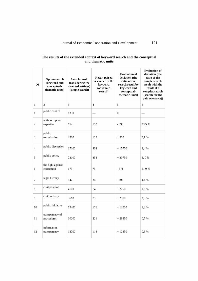
Journal of Economic Cooperation and Development 121
The results of the extended context of keyword search and the conceptual
and thematic units
№
Option search
(keyword and
conceptual-
thematic units)
Search result
(considering the
received settings)
(simple search)
Result paired
relevance to the
keyword
(advanced
search)
Evaluation of
deviation (the
ratio of the
search result by
keyword and
conceptual-
thematic units)
Evaluation of
deviation (the
ratio of the
simple search
result with the
result of a
complex search
(search for the
pair relevance))
1 2 3 4 5 6
1 public control
1350 — 0 —
2
anti-corruption
expertise 652 153 - 698 23,5 %
3
public
examination 2300 117 + 950 5,1 %
4 public discussion
17100 402 + 15750 2,4 %
5 public policy
22100 452 + 20750 2, 0 %
6
the fight against
corruption 679 75 - 671 11,0 %
7 legal literacy
547 24 - 803 4,4 %
8 civil position
4100 74 + 2750 1,8 %
9 civic activity
3660 85 + 2310 2,3 %
10 public initiative
13400 178 + 12050 1,3 %
11
transparency of
procedures 30200 221 + 28850 0,7 %
12
information
transparency 13700 114 + 12350 0,8 %

122 Determination of the Degree of Development and the Impact of the
Information Environment on the Formation of a System of Social Control
in Procurement Under the Russian Contract System
(Method of Content Analysis of Information Resources on the Internet)
The results of calculating the ratio of the results of simple and complex
searches can be interpreted as follows. Application of a complex search
query, comprising several phrases are always significantly narrows the
search area and the number of search results, respectively, since the
number of search results inversely proportional to the search terms. For
example, the number of results simple search on the word "fairy tale"
gives 23,900,000 results. Using complex search for "tales of Pushkin" is
1 300 000 results. The deviation in this case is 5.4%, despite the fact that
a simple search for "Pushkin" shows the result in 13.9 million hits. The
ratio of the result of complex and simple search can be very different,
vary from 100% to close to zero, but the main value of establishing a
relationship is that it gives definition to diagnose the connection
between the search queries.
To conduct content analysis, we define the following relation between
the result of complex and simple search. The smaller the amount of
deviation of the results of complex search (pair relevance - two phrases)
on the number of results on the appropriate conceptual and thematic
unity (ie, the larger percentage), the more stable relationship is observed
between the keywords "social control" and a separate conceptual and
thematic unit. In this case the deviation shows that the number of results
the search query in two phrases (keywords and conceptual-thematic
unity) slightly corrects (narrows) the number of results a search query on
a specific conceptual and thematic unity. Thus, a large number of
coincidences between the results of simple and complex research
suggests that in the information space, there is a significant number of
pages in the content of which there are complex search phrases desired
interconnected common sense.
Conversely, the greater the amount of deviation of the results of a
complex search (steam relevance - two phrases) on the number of results
on the appropriate conceptual and thematic unity (i.e., the smaller
percentage), the less stable relationship is observed between the
keywords "social control" and separate conceptual and thematic unity.
This dependence shows that the result of a complex search in large
communication distorts the results of a simple search on the conceptual
and thematic unity. For the purpose of this content analysis of this result
indicates that the number of pages of information and communication on
the Internet, which are the same and have the common sense of the

Journal of Economic Cooperation and Development 123
phrase keywords "social control" and the phrase on a separate
conceptual and thematic unity, slightly. This result demonstrates a low
degree of correlation between complex search phrases.
Because the number of conceptual-thematic units is defined as the
absolute number of the final sample, the analysis of the ratio of the
complex and the simple search is carried out exclusively within the
sample without relations with other possible search queries. Analyzing
the results of the extended context search in the table 3, it should be
noted that the total number of results regarding the high degree of
dependence is observed for the conceptual and thematic units' anti-
corruption expertise "(23.5%)," Fighting Corruption "(11.0% deviation)
and "public examination" (5.1%). All other results show a deviation of
5% or less. Indicators with an average degree of dependence (from 5%
to 2%) should be attributed to the following indicators conceptual-
thematic units "legal literacy" (4.4%), "public discussion" (2.4%), "civic
engagement" (2.3%), "public policy" (2.0%). Low degree of dependence
(below 2%) was observed for the conceptual and thematic units
"citizenship" (1.8%), "public initiative" (1.3%), "information
transparency" (0.8%), "the transparency of procedures "(0.7%).
If we compare the results obtained by the definition of semantic
isolation conceptual-thematic units of keywords and the results to
determine the quality of the connection between the conceptual and
thematic units and keywords, you can estimate the direction of the
relation between the results (Table 4)

124 Determination of the Degree of Development and the Impact of the
Information Environment on the Formation of a System of Social Control
in Procurement Under the Russian Contract System
(Method of Content Analysis of Information Resources on the Internet)
Correlation of the results found for the extended context of semantic
degree of isolation and connection quality
The degree of semantic
isolation results simple
search
The results of
calculating the ratio of
the results of simple
search
The results of
calculating the ratio of
the results of simple
and complex search
The quality of
communication
between the results of
simple and complex
search
The high degree of sense
of separateness
"Transparent
procedures", "public
policy", "public
discussion",
"information
transparency", "public
initiative"
"Anti-corruption
expertise", "anti-
corruption", "public
examination"
High-quality
communication
The average degree of
sense of separateness
"Citizenship", "civic
engagement", "public
examination"
"Legal literacy", "public
discussion", "civic
engagement", "public
policy"
Average quality
communication
Low degree of sense of
separateness
"Anti-corruption
expertise", "anti-
corruption", "legal
literacy"
"Citizenship", "public
initiative", "information
transparency",
"transparent procedures"
Low quality
communication
Analysis of the results tables 4 to determine the presence inversely
proportional relationship between the degree of isolation of conceptual-
semantic unit’s thematic content analysis and quality of communication
between the key words and concepts and thematic units. One cannot
speak of the absolute values of the inverse proportional relationship, but
a definite trend correlation results advanced context sensitive searches
traced. Errors occur due to errors of the order of distribution of the
search results between levels (error application techniques comparison
purposes), and also due to the error operation of search when
determining the relevance of search results steam.
Establish the presence or absence of communication will allow
conducting correlation and regression analysis. To do this, we need to
calculate the correlation, linear regression to build and test the
hypothesis according to two related quantities. In our case, the
associated values are the results of a simple search and complex search
results. Recall that the condition is a simple search advanced contextual
search on the set parameters in one phrase (keyword "social control" and
the conceptual and thematic units). In turn, the complex search condition

Journal of Economic Cooperation and Development 125
is advanced contextual search on the set parameters on the phrase pair,
which consists of a keyword and a separate conceptual and thematic
units. For correlation and regression analysis is not required to use the
results of simple keyword search, analysis is carried out using only the
results of a simple search on the conceptual and thematic units. Thus,
there is a related sample of 11 pairs of values - the results of a simple
search (X) and the results of complex search (Y). Required:
calculate the correlation coefficient;
test the hypothesis according to the random variables X and Y,
with a confidence level of 98-99% (significance level - 0,02-0,01
respectively);
to calculate the coefficients of the linear regression;
build a scatter plot (correlation field) and the graph of the
regression line.
Calculation of the correlation coefficient.
The correlation coefficient is a measure of the probability of mutual
influence of two random variables. The correlation coefficient can take
specific values (-1 to +1). If the absolute value is closer to 1, it indicates
a strong connection between the values, and if closer to 0 - what it says
about the weak coupling or its absence. If the absolute value of the
correlation coefficient takes a value of 1, then we can talk about the
functional connection between random variables, that is, when one value
can be expressed by other means of a mathematical function. Compute
the correlation coefficient can be as follows:
,
xy x y
xy
x y
M MM
SSR
(1.1) To calculate the correlation coefficient is necessary to make a
table of values xk2, yk2 and xkyk (Table 5).

126 Determination of the Degree of Development and the Impact of the
Information Environment on the Formation of a System of Social Control
in Procurement Under the Russian Contract System
(Method of Content Analysis of Information Resources on the Internet)
The values for the calculation of the correlation coefficient
Number
of search
options
(k)
Context search
options
conceptual and
thematic units
The result
of a simple
search (X)
The result of
a complex
search by
relevance (Y)
𝐗𝟐 𝐘𝟐 XY
1 2 3 4 5 6 7
1 anti-corruption
expertise
652 153 425104 23409 99756
2 public
examination
2300 117 5290000 13689 269100
3 public
discussion
17100 402 292410000 161604 6874200
4 public policy 22100 452 488410000 204304 9989200
5 the fight against
corruption
679 75 461041 5625 50925
6 legal literacy 547 24 299209 576 13128
7 civil position 4100 74 16810000 5476 303400
8 civic activity 3660 85 13395600 7225 311100
9 public initiative 13400 178 179560000 31684 2385200
10 transparency of
procedures
30200 221 912040000 48841 6674200
11 information
transparency
13700 114 187690000 12996 1561800
THE SUM OF
THE RESULTS 108438 1895 2096790954 515429 28532009
It is necessary to carry out calculations using formulas 1.2. and 1.3. The
calculations are shown in Table 6.
1
1 n
kxk
xn
M
, 1
1n
kyk
yn
M
, 1
1n
k kxyk
xyn
M
(1.2)
2 2 2
1
1n
k xxk
x Mn
S
, 2 2 2
1
1n
k yyk
y Mn
S
(1.3)

Journ
al o
f E
conom
ic C
ooper
atio
n a
nd D
evel
opm
ent
1
27
Cal
cula
tio
n o
f q
uan
titi
es b
y t
he
form
ula
s 1
.2.
and
1.3
.
№
The
proc
edur
e fo
r
calc
ulat
ing
Mx
My
S x2
S y
2
Mx
y
S x2
∗ S y
2
√S x
2∗
Sy2
R
xy
1 Ca
lcul
atio
n M
x;
My
; Mx
y; (
divi
ding
the
sum
of
the
resu
lts o
n th
e
num
ber
of s
earc
h
optio
ns)
9036
,5
157,
9166
6666
67
2377
667,
4166
6667
2 Ca
lcul
atio
n M
x;
My
; Mx
y;
(cal
cula
tion
of a
squa
re v
alue
Mx;
My
; Mx
y)
8165
8332
,25
2493
7,67
3611
111
2
5653
3023
4427
8,36
3 Ca
lcul
atio
n S x
2; S
y2;
(div
idin
g th
e su
m o
f
the
squa
re o
f th
e
resu
lts o
n th
e
num
ber
of s
earc
h
optio
ns a
nd
subt
ract
ing
the
squa
re s
um o
f th
e
resu
lts)
9307
4247
,25
1801
4,74
3055
5556

128 D
eter
min
atio
n o
f th
e D
egre
e of
Dev
elopm
ent
and t
he
Impac
t of
the
Info
rmat
ion E
nvir
on
men
t o
n t
he
Fo
rmat
ion
of
a
Syst
em o
f S
oci
al C
ontr
ol
in P
rocu
rem
ent
Under
the
Russ
ian C
ontr
act
Syst
em
(M
ethod o
f C
onte
nt
Anal
ysi
s of
Info
rmat
ion R
esourc
es o
n t
he
Inte
rnet
)
Cal
cula
tio
n o
f q
uan
titi
es b
y t
he
form
ula
s 1
.2.
and
1.3
. (C
ont.
)
4
Calc
ulat
ion
S x2
∗ S y
2
(пр
ои
звед
ени
е
S x2
на
S y2
)
1676
7086
4929
8
5 Sq
uare
root
extr
actio
n (t
he
squa
re ro
ot o
f th
e
prod
uct
of S
x2∗
S y2
)
1294
877,
8511
1106
6 Ca
lcul
atio
n of
the
valu
e of
the
corr
elat
ion
coef
ficie
nt
(Rx
y)
(Mx
y−
Mx*
My)/√
S x2
∗ S
y2
0,73
4164
5836
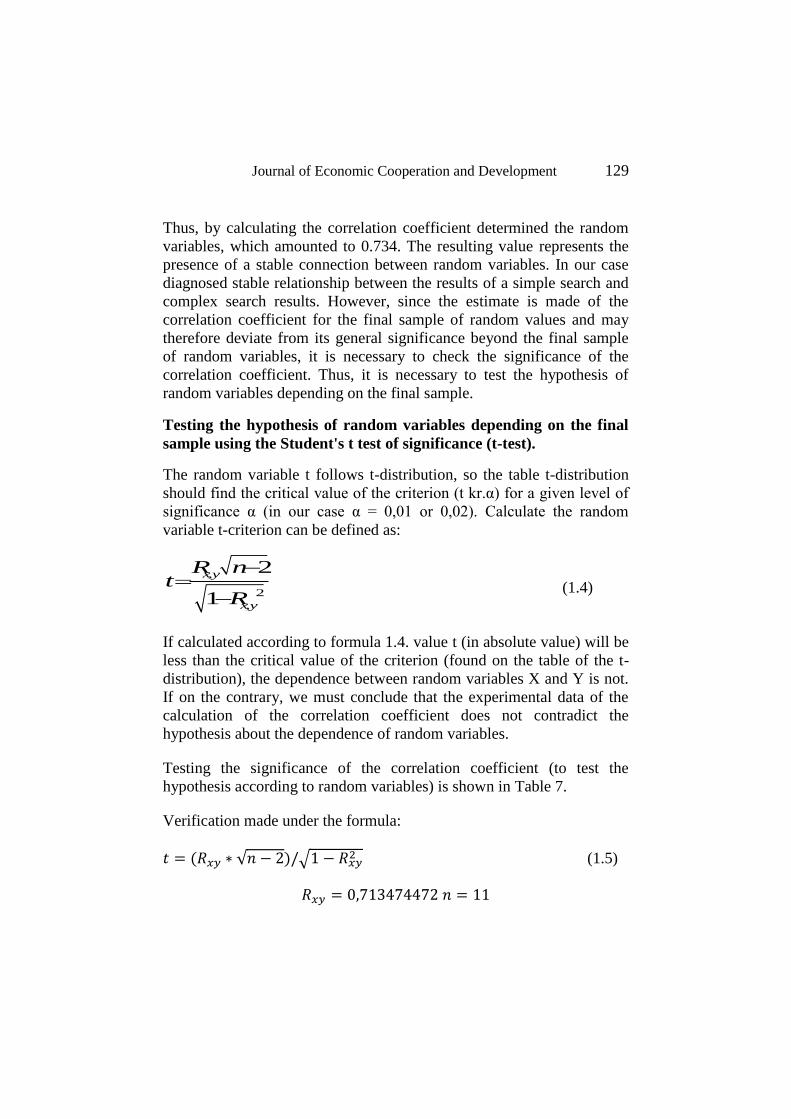
Journal of Economic Cooperation and Development 129
Thus, by calculating the correlation coefficient determined the random
variables, which amounted to 0.734. The resulting value represents the
presence of a stable connection between random variables. In our case
diagnosed stable relationship between the results of a simple search and
complex search results. However, since the estimate is made of the
correlation coefficient for the final sample of random values and may
therefore deviate from its general significance beyond the final sample
of random variables, it is necessary to check the significance of the
correlation coefficient. Thus, it is necessary to test the hypothesis of
random variables depending on the final sample.
Testing the hypothesis of random variables depending on the final
sample using the Student's t test of significance (t-test).
The random variable t follows t-distribution, so the table t-distribution
should find the critical value of the criterion (t kr.α) for a given level of
significance α (in our case α = 0,01 or 0,02). Calculate the random
variable t-criterion can be defined as:
,
2
,
2
1
xy
xy
R nt
R
(1.4)
If calculated according to formula 1.4. value t (in absolute value) will be
less than the critical value of the criterion (found on the table of the t-
distribution), the dependence between random variables X and Y is not.
If on the contrary, we must conclude that the experimental data of the
calculation of the correlation coefficient does not contradict the
hypothesis about the dependence of random variables.
Testing the significance of the correlation coefficient (to test the
hypothesis according to random variables) is shown in Table 7.
Verification made under the formula:
𝑡 = (𝑅𝑥𝑦 ∗ √𝑛 − 2)/√1 − 𝑅𝑥𝑦2 (1.5)
𝑅𝑥𝑦 = 0,713474472 𝑛 = 11

130 Determination of the Degree of Development and the Impact of the
Information Environment on the Formation of a System of Social Control
in Procurement Under the Russian Contract System
(Method of Content Analysis of Information Resources on the Internet)
Test the significance of the correlation coefficient
Indicator Correlation
factor
(𝑅𝑥𝑦)
𝑅𝑥𝑦2 Number
of earch
options
(n)
Number of
degrees of
freedom of
Student's
(n-2)
√𝑛 − 2 Calculation
√1 − 𝑅𝑥𝑦2
Calculation t
criterion
value of
the index
0,7341645836 0,5389976358 11 9 3 0,6789715489 3,2438675147
Analyzing the results of testing the hypothesis according to random
variables should be noted that with high probability the experimental
data for the calculation of the correlation coefficient does not contradict
this hypothesis. This means that the result of the calculation of the
correlation coefficient of a stable correlation between random variables
finite sample can be extended to a general correlation coefficient outside
the final sample of random variables. To further study the nature of the
relationship between random variables necessary to calculate the
coefficient of the linear regression equation.
Calculation of the coefficient of the linear regression equation.
Linear regression equation is an equation of the line, about describing
the dependence between random variables X and Y. If we consider that
the value of X is free, and Y - a function of x, the regression equation
should be written as follows:
𝑌 = 𝑎 + 𝑏 ∗ 𝑀𝑥 (1.6)
In this case, the value of X (the simple search results) is indeed free
value, in turn, the magnitude of Y (complex search results) is completely
dependent on the value of X as a basis of the search results is the
complex combination of keywords and a notional focal units.
To calculate the coefficients of the linear regression - permanent
regression coefficient (a) and variable regression coefficient (b), it is
necessary to make calculations using formulas 1.7 and 1.8.
𝑏 = 𝑅𝑥𝑦𝛿𝑦
𝛿𝑥= 𝑅𝑥𝑦
𝑆𝑦
𝑆𝑥 (1.7)
𝑎 = 𝑀𝑦 − 𝑏 ∗ 𝑀𝑥 (1.8)

Journal of Economic Cooperation and Development 131
The procedure for calculating the coefficients of the linear regression is
shown in Table 8.
Calculation of the linear regression equation: 𝑌 = 𝑎 + 𝑏 ∗ 𝑋
Procedure for calculating the linear regression equation.
𝑀𝑥 𝑀𝑦 𝑅𝑥𝑦 𝑆𝑥2 𝑆𝑦
2 𝑆𝑥2/𝑆𝑦
2 √𝑆𝑥
2/𝑆𝑦2
coefficien
t a
coefficient
b
903
6,5
157,91666
66667
0,73416
45836
930742
47,25
18014,7430
555556
0,00019
35524
0,01391
23108
0,01021
39258
65,61852
58786
Linear regression equation has the form: 𝑌 = 65,6185258768 + 0,0102139258 ∗ 𝑋
To evaluate the prediction error is also necessary to make calculations,
the procedure for calculating prediction error Y for a given value of x in
accordance formulated 1.9 and 1.10 shown in the table.
𝛿𝑦/𝑥 = 𝛿𝑦√1 − 𝑅𝑥𝑦2 = 𝑆𝑦√1 − 𝑅𝑥𝑦
2 (1.9)
𝛿𝑦/𝑥 = 𝛿𝑦/𝑥
𝑀𝑦100% (1.10)
An error estimate for the linear regression equation.
Absolute error: 𝜎𝑥/𝑦 = √𝑆𝑥2 ∗ √1 − 𝑅𝑥𝑦
2
Relative error: 𝛿𝑦/𝑥 = (𝜎𝑥𝑦
𝑀𝑦) ∗ 100%
The calculation of prediction error for a given value Y X
𝑆𝑦 𝑅𝑥𝑦2 𝜎𝑥/𝑦 𝛿𝑦/𝑥
134,219011528 0,5389976358 91,1308901462 57,71%
Error equation:
𝜎𝑥/𝑦 = 91,1308901462
Further investigation of the dependence of random variables involves the
construction of scatter plots (correlation of the field) and the graph of the
regression line. The scattering diagram - a graphical representation of the
corresponding pairs of random variables X and Y in the form of points in

132 Determination of the Degree of Development and the Impact of the
Information Environment on the Formation of a System of Social Control
in Procurement Under the Russian Contract System
(Method of Content Analysis of Information Resources on the Internet)
a plane with coordinates axes X and Y. In the same coordinate system and
construct a graph of the regression line. A special feature is the choice of
construction diagrams and scale of initial points on the axes, provides a
visual diagram. The procedure and results of the calculation of the
regression line points: point A with coordinates (Хmin; Ymin) and point B
with coordinates (Хmax; Ymax) is shown in Table 9.
Verifying plotting the regression line is performed by applying a
coordinate system point average values of the random variables X and Y
coordinates (Мх;Му).
Calculation of the regression line and the points on the linear
regression equation.
𝑌 = 65,6185258768 + 0,0102139258 ∗ 𝑋
Compute point on the regression line equation of the linear regression
Хmin Ymin Хmax Ymax
547 71,2055433074 30200 374,0790860334
Coordinates of the regression line:
A (547;71) ; B (30200;374)
Scatter plot and graph the regression line shown in Figure 1.
Figure 1. Scatter diagram (correlation field) and the graph of the regression line
B
A
Y
X
5
4
3
1
0
2
3 6
0
9 12 15 18 21 24 27 30

Journal of Economic Cooperation and Development 133
The distribution of points in pairs of random variables shows that they
correspond to the direction of the graph of the regression line, however,
the degree of approximation to the scattering points of the regression
line is not sufficient, which reduces the quality of the linear regression
equation. However, validation plotting a linear regression on the
coordinate system point average values of the random variables X and Y
coordinates (Мх;Му) showed perfect agreement with the coordinates of
the point (Мх;Му) generated from the linear regression line. Thus, the
lack of proximity of the scattering points (coordinates of points on the
results of a pair of simple and complex search) is due to an insufficient
number of random variables finite sample.
Findings
The results of correlation and regression analysis confirmed the presence
of a stable connection between the results of advanced context sensitive
searches as part of the content analysis showed an association between
the results of keyword search and conceptual and thematic units. It
speaks to the uniformity of information flow, which brings together
thematic pages on the Internet for all investigated units of content
analysis. Thus, the purpose of the content analysis by determining the
degree of development and the impact of the information environment
on the formation and implementation of methods of social control in
procurement under the Russian contract system achieved. The results of
the content analysis can be used to further study the dynamics of
changes in the interim results of content analysis to determine the areas
of development, structure and content of the flow of information on
topics related to information support of public control in procurement
and contract system development.
134 Determination of the Degree of Development and the Impact of the
Information Environment on the Formation of a System of Social Control
in Procurement Under the Russian Contract System
(Method of Content Analysis of Information Resources on the Internet)
References
The Federal Law of 21.07.2014 № 212-FL "On the basis of public
control in the Russian Federation"
The Federal Law of 05.04.2013 № 44-FL (ed. By 04.06.2015) "On the
contract system in the procurement of goods, works and services for
state and municipal needs"

Journal of Economic Cooperation and Development, 37, 3 (2016), 135-174
Bilateral Trade through Official Channel between India and
Bangladesh: An Analysis with the Use of Time Series Forecasting
Models
Muhammad Mahboob Ali1 and Anita Medhekar
2
Bilateral trade between India and Bangladesh will be mutually beneficial to
both the countries and improve welfare as per trade theory. This study has tried
to forecast impact of trade between two countries considering the time period
1991-2014.The researchers compared Autoregressive Moving Average
(ARMA) and Autoregressive Integrated Moving Average Model (ARIMA)
after testing the significance of Augmented Dicky fuller model’s intercept of
explanatory variables.While using ARIMA model the study found that best-fit
estimates were exports to India. However, forecasting indicates that import
from India to Bangladesh also had a positive impact over the time period 1991-
2014.By engaging in bilateral trade with India, Bangladeshi producers and
suppliers ought to be concerned about attaining long term sustainability in their
business, by improving quality of the products so that export can be raised in a
competitive manner. Market access to India will be beneficial only with having
competitive advantage, in bilateral trade. To export products, India should
allow duty free access to certain products from Bangladesh in which it has
competitive advantage. To maintain Pareto optimality in the bilateral trade,
Bangladesh should import products from India at competitive prices. This will
help to promote and nurture bilateral trade relations, ensure sustainability of
business and mutually benefit both the countries through free trade agreement.
1. Introduction
Trade between India and Bangladesh has a long history. Besides
bilateral trade with India, informal trade also plays an important role in
Bangladesh. Trade between these two countries is not only creating
value but acting as a value chain, which is a corner stone for improving
1 Professor, Faculty of Business and Economics, and Director, Institutional Quality
Assurance cell, Daffodil International University, Bangladesh. The author is former
Vice Chancellor of Presidency University, Bangladesh. Email: [email protected] 2 Senior Lecturer of Economics, Central Queensland University, Australia.
Email: [email protected]

136 Bilateral Trade through Official Channel between India and
Bangladesh: An Analysis with the Use of Time Series Forecasting Models
bilateral relationships. However, given the geographical proximity,
relationship with India is historical, cultural, social and cordial to have
any significant impact on the two economies. Therefore increasing bi-
lateral trade between the two neighbouring countries is very essential for
employment generation, economic development and growth.
Furthermore, according to Ankit(2015) India’s foreign policy would
appear to the Commonwealth Relations Office to be ‘a picture not only
of an ever enlarging sphere of regional co-operation but also of
expanding Indian ambitions’ is somewhat not valid in this century .Both
the countries should maintain diplomatic relationship not only for geo-
political reasons to mutually benefit from each other to ensure
sustainable economic development and growth through South Asian
Association of Preferential Trade Agreements (SAPTA)and the Bay of
Bengal initiative for Multi-Sectorial Technical and Economic
Cooperation (BIMSTEC),but also to fight against global and regional
terrorism, irradiate poverty, and improve welfare for millions. There are
three factors that are identified in case of Bangladesh, which have a
negative influence for encouraging trade: ease of doing business,
unrecorded informal trade and high transaction cost of engaging in trade.
(1) Ease of Doing Business: ‘Ease of Doing Business Index (EDBI) for
Bangladesh in 2014 was last measured at 173 and for India 142 out of
189 countries [see World Bank, (2014)]. As such Bangladesh still has a
long way to go for further development of easing business procedure,
which is to provide business friendly environment in this competitive
global state of the 21stcentury. Likewise India should also reduce its
protectionist trade policies between the South Asian nations. (2)
Informal Trade: World Bank (2015) stated that since the independence
in December 1971, there has been a substantial increase in informal
unrecorded trade across the India-Bangladesh land borders, and a
number of studies both in Bangladesh and in India have dealt with
different aspects of it. (3) Transaction Cost: The trade diverted through
the formal channels provide customs revenue, and this would be higher
if administrative and other reforms reduce the scope for corrupt
practices. Better infrastructure, faster clearance times and reduced
transaction costs would also improve the prospects of Bangladesh
exporters finding niche market in India, especially if they rely on
importing inputs from India, where there is two way border crossing for
trade [see World Bank (2015)].

Journal of Economic Cooperation and Development 137
Key factors that unite Bangladesh and India as identified by
Government of India (2013) are the following:
Both the countries share a common heritage- language,
civilisation, colonial history, social and, economic history.
India and Bangladesh have common interest and share a
common heritage for music, classical dance, literature, poetry
and the creative arts.
With Bangladesh, India shares not only a common history of
struggle for freedom and liberation but also enduring feelings of
both fraternal as well as family ties.
India played a major role in emergence of Independent
Bangladesh during the 1971 war, and it was also the first country
to recognize Bangladesh as a separate independent nation.
There have been major issues such as illegal migration, border,
water sharing disputes, Moore Island, which have had a negative
impact on bilateral trade in the recent years.
Ahmed(2015) argued that the Indian Prime Minister Narendra Modi
visited Bangladesh in June, 2015 for a mere 36 hours, but left an impact,
big enough to wipe away mistrust that had crept in the Indo-Bangladesh
relationship over the decades. The Indian Express (2015) quoting Joshi,
President of the Federation of Industry and Commerce, North-Eastern
Region of India commented that the agreement during Modi’s visit to
Bangladesh was on infrastructure development, which focuses on
connectivity by road, rail, air, river, sea, transmission lines, petroleum
pipelines and digital links. This development will have a multiplier
effect on the economy and provide a real boost to cross-border trade
between Bangladesh and North Easternpart of India. Sharma (2015)
reported that an investment of US$ 2 billion line of credit is extended to
Bangladesh, further to current US$ 1 billion. Most importantly, if
boundary disputes aresettled then the foundation to build trust for
infrastructure development is laid. This will be mutually beneficial for
trade between the two countries. During the visit most of the 22 bilateral
agreements were signed aimed at boosting trade and transport links.
Further, Indian corporate entities like Reliance Power and Ambani
Group signed agreements to invest around $5 billion which will help
Bangladesh to generate extra 4600 MW of power, to meet its electricity
demand.

138 Bilateral Trade through Official Channel between India and
Bangladesh: An Analysis with the Use of Time Series Forecasting Models
Main objective as neighbouring countries should be to try to resolve all
cross-border disputes peacefully, without forgetting the 1971 war of
independence and soldiers who sacrificed their life from both sides for
independence, in order to mutually benefit from trade relationships and
maintain peace and harmony across border for economic development
and growth. According to sources of ministry of external affairs, there
has been progress in Indo-Bangladesh relations as per the following
initiatives taken by the government on both sides:
High level of recent contacts at government level, exchange and
visits.
Wide ranging people-to-people interaction at cultural and social
networking level.
Indian High commission in Bangladesh issues about half a
million visas every year and thousands of Bangladeshi students
study in India on self-financing basis.
Recipients of over one hundred annual Government of India
scholarships.
Bangladesh Prime Minister Sheikh Hasina in 2011, along with
Indian Prime Minister Dr. M. Singh announced the
commencement of 24-hour access across the Tin Bigha corridor
to Dahagram and Angorpota enclaves, as well as duty-free
import of 46 textile items (subsequently expanded to all items,
except 25 items) from Bangladesh to India.
Common vision for rural development, health, education, clean
drinking water and sanitation, people’s empowerment and
economic development issues discussed at the government level.
India has always helped Bangladesh in its hour of need with aid
worth over Taka 250 crore (over US $ 37 million) to help it cope
with natural disasters and floods in 2007-08.
Supply of 1,000 MT of skimmed milk powder, and 40,000
Million Tons of rice.
India completed and handed over 2,649 core shelters in the
affected villages in Bagerhat district in southern Bangladesh.
Line of Credit Agreement was signed in Dhaka on August 7,
2010 between EXIM Bank of India and Government of
Bangladesh. India has extended a line of credit of US$1 billion to
Bangladesh for a range of infrastructure and development
projects, including railway infrastructure, supply of BG

Journal of Economic Cooperation and Development 139
locomotives and passenger coaches, procurement of buses, and
dredging projects.
January 29 -2012, NTPC and BPDB set up a Joint Venture for
the establishment of a 1320-MW coal-based power plant in
Bagerhat district, Khulna at an estimated cost of $1.5 billion and
is to be commissioned by 2016.
India offers 100 places under ITEC and 35 under Technical
Cooperation Scheme of Colombo Plan every year to Bangladesh.
In the last three years (2006-07 to 2009-10), 414 participants
from Bangladesh underwent training in India under ITEC
Programme and Technical Cooperation Scheme of Colombo
Plan. Government of India gave Muktijoddha Scholarship to 200
Higher Secondary-level students and 478 Graduate-level
students. Further, in 2011 three Bangladesh Diplomats were also
imparted training at Foreign Service Institute in India.
Such bilateral Cultural Exchange Programme (CEP) 2009-2012 between
Bangladesh and India provides the platform for fruitful exchanges; given
the shared history and commonality of language; cultural exchanges
form an important bond of friendship between the people of two
countries. Special emphasis has been laid on promotion of cultural
exchanges in the fields of music, theatre, art, sports, painting and books,
such as: Joint celebrations of 150th anniversary of Rabindranath Tagore;
to honour the Indian friends of Bangladesh for their contribution to the
1971 Liberation War; through student-teacher exchange programmes
and reciprocal programmes of cooperation; promote people to people
exchanges, 100 scholarships are being granted by ICCR every year to
students from Bangladesh, and; In the year 2013-14, totalexport from
Bangladesh to India was worth US$ 457 Million, whiletotal import from
India to Bangladesh was worth US$ 5514 Million and total trade with
India was US$ 5971 Million.
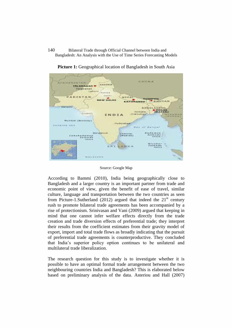
140 Bilateral Trade through Official Channel between India and
Bangladesh: An Analysis with the Use of Time Series Forecasting Models
Picture 1: Geographical location of Bangladesh in South Asia
Source: Google Map
According to Bammi (2010), India being geographically close to
Bangladesh and a larger country is an important partner from trade and
economic point of view, given the benefit of ease of travel, similar
culture, language and transportation between the two countries as seen
from Picture-1.Sutherland (2012) argued that indeed the 21st century
rush to promote bilateral trade agreements has been accompanied by a
rise of protectionism. Srinivasan and Vani (2009) argued that keeping in
mind that one cannot infer welfare effects directly from the trade
creation and trade diversion effects of preferential trade; they interpret
their results from the coefficient estimates from their gravity model of
export, import and total trade flows as broadly indicating that the pursuit
of preferential trade agreements is counterproductive. They concluded
that India’s superior policy option continues to be unilateral and
multilateral trade liberalization.
The research question for this study is to investigate whether it is
possible to have an optimal formal trade arrangement between the two
neighbouring countries India and Bangladesh? This is elaborated below
based on preliminary analysis of the data. Asteriou and Hall (2007)
Journal of Economic Cooperation and Development 141
argued that ARMA models can only be made on time series Yt that are
stationary. Time series is not constant over time, which means that the
series are non-stationary. If, after first differencing, a series is stationary,
then the series is also called integrated to order one, and denoted 1(1) –
which completes the abbreviation ARIMA.This paper is structured as
follows. Following the introduction, section two provides literature
review. Section three provides methodology followed by section four
which discusses the results of empirical analysis. Section five provides
conclusions, implications and future research directions.
2. Literature Review
Krugman (1980) rightly asserts that if two countries have the same
composition of demand, the larger country will be a net exporter of the
products whose production involves economies of scale. Bangladesh
capacity to attain competitiveness in trade with India is a big question,
due to low capacity building, as well as lack of competitiveness in the
formal trade and huge balance of trade deficit. Wangwe (1993) elements
of the new trade theories which are relevant to trade and development
issues pertaining to developing countries can be applied to India and
Bangladesh: the conception of process of narrowing the technology gap
between the developed and developing countries; implications on the
conception of North-South technology-related negotiations; therole of
multinational activities in the developing countries; intra-south trade and
investments; industrial dynamics and attainment of competitiveness; and
the role of governmentpolicy in enhancing competitiveness in the
economy. Etheir (2001) described that countries tend to trade a lot with
their neighbours, so it is sometimes said that current regional initiatives
between the two countries, often involving neighbours, are therefore
likely to be benign. Hassan (2002), emphasised that the geographical
proximity of India along with the increasing familiarity of Bangladesh’s
importers to India’s production capacities, which in recent years have
become globally competitive both in terms of price as well as quality
has made Indian products increasingly competitive in Bangladesh’s
market. He suggested that the only way to increase the volume of intra-
regional trade and reduce the trade deficit with India, Bangladesh should
take the following steps: devalue its currency, seek reduction in tariff
and non-tariff barriers on exports to India, stop cross-border smuggling
activities, eliminate structural and political rigidities and conflicts,
encourage more Indian investment into Bangladesh and make the
142 Bilateral Trade through Official Channel between India and
Bangladesh: An Analysis with the Use of Time Series Forecasting Models
SAPTA more meaningful, effective and operational tool to reap the
benefits from integration.
Moreover there are positive benefits to the countries and the world, by
engaging in regional, bi-lateral and multi-lateral free trade [see Khan
(1999), Dutta (1999),and Jain (1999)]. However, intra-SAARC trade is
very small (Hassan, Mehanna and Bashar 2001) compared to other
regional blocks like ASEAN and NAFTA. Further, Hassan (2001)
empirical study, using the gravity model of international trade for years
1996-1997, concluded that the proportion of intra-regional trade
between the South Asian block of countries is very small due to “normal
outcomes or unexplored opportunity” (p.264), and if increased, can have
significant welfare improving benefits along with implementing
supporting policies by the governments to encourage preferential trade
agreement under South Asian Association of Regional Cooperation
(SAARC).Hassan (2001) results supports the argument that small
countries depend more on trade then larger and diversified countries;
poor countries trade less with each other, than with the rich countries,
and countries sharing common border, trade more with each other.
Therefore regional economic cooperation between these two countries
should be encouraged, given the similar social-economic and cultural
conditions. The major export items from a small country Bangladesh, to
a comparatively large country India within the SAARC region as
recorded by Dhaka Chamber of Commerce are the following: Woven
Garments; Knitwear; Home Textile; Agri-Products; Frozen Food;
Leather & Leather Products; Footwear; Raw Jute; Jute Goods; Bicycle
Major Import Items to Bangladesh from India are: Cotton (all types),
cotton yarn / thread and cotton fabrics; Cereals; Vehicles other than
railway or tramway rolling- stock and parts and accessories thereof;
Residues and waste from the food industries, prepared animal fodder;
Nuclear reactor, boilers, machinery and mechanical appliances parts;
Iron and steel; Edible vegetables and certain roots and tubers; Organic
chemicals ;Mineral fuels, mineral oils and products of their distillation,
bituminous substances, mineral waxes; Plastics and articles thereof;
Tanning or dyeing extracts, tannins and their derivatives, dyes, pigments
and other colouring matter, paints and varnishes, putty and other
mastics, inks; Salt, sulphur, earths and stone, plastering materials, lime
and cement [see Dhaka Chamber of Commerce (2015)].
Journal of Economic Cooperation and Development 143
Further items exported by Bangladesh are: Electrical machinery and
equipment and parts thereof, sound recorders and reproducers, television
image and sound recorders and producers and parts and accessories of
such articles; Man-made staple fibers; Dairy produce, birds' eggs natural
honey, edible products of animal origin, not elsewhere specified or
included; Coffee, tea, mate and spices; Rubber and articles thereof ;
Edible fruit and nuts, peel of citrus fruit or melons; Man-made
filaments; strip and the link of man-made textile materials ;Aluminium
and articles thereof; Knitted or crocheted fabrics; Inorganic chemicals,
organic or inorganic compounds of precious metal, of rare earth metals,
of radioactive elements for isotopes; Paper and paper board, articles of
paper pulp; Essential oils and resinoids; perfumery, cosmetic or toilet
preparation; Oil seeds and oleaginous fruits; miscellaneous grains, seeds
and fruits; industrial or medicinal plants; straw and fodder and
Pharmaceutical products [see Dhaka Chamber of Commerce (2015)].
However, the largest trading partners of Bangladesh are European Union
and North America in terms of legal exports and India for legal imports
since late 1990’s [see Hassan (2001)].
World Bank also reported in the year 2002 surveys that smuggled goods
were imported from India to Bangladesh during 2002/03 were worth
approximately $500 million, or about 40% of recorded imports from
India, and approximately 30% of total imports (recorded plus smuggled)
from India[see World Bank, (2006)].Pohit and Taneja (2003) argued that
informal trade continues to thrive because the transacting environment
of formal and informal trading arrangements gives rise to lower
transaction costs in the informal channel. Srinivasan (2002) depicted
that unless the transacting environment improves significantly for
formal traders, informal trade will continue to co-exist along with formal
trade.
Hossain and Rashid (1999) argued from their empirical study, that
Bangladesh’s trade with India is neither fair nor competitive due to trade
barriers .Bhagwati (1995) described that the restrictiveness of trade
barriers is therefore likely to have increased as required. Such elasticity
and also selectivity are in fact characteristics of the “administered”
protections embodied in antidumping actions and Voluntary Exports
Restraints (VERs) which make them both a preferred instrument of
protection by industry and also a serious barrier to free trade. Further,
the transacting environment of formal trade agreement between India

144 Bilateral Trade through Official Channel between India and
Bangladesh: An Analysis with the Use of Time Series Forecasting Models
and Bangladesh indicates that the inefficiencies of the trade regimes
give rise to rent seeking activities by the authorities, bureaucrats and
politicians. That is formal traders prefer to use mechanisms of informal
trading to settle disputes[see Pohit and Taneja (2003)].
Ahmed (2006) very rightly pointed out that firstly, Bangladesh-India
relationship is faced with certain puzzles which need to be addressed
professionally and without any animosity. Secondly,the regional and
global scenarios have transformed the Indo-Bangladesh relationship in
several key areas, both for the good and the bad, therefore, not fully
realising the benefits of bilateral trade between neighbours who have
significant historical advantage. Khan and Khan (2003) suggest to have
open regionalism, that is outward oriented development policies by
merging regional trading blocs and harmonising domestic economic
policies with global economic policies, and extend the SAARC
integration to West Asia in Iran, to Burma in the East, to benefit from
trade, investment opportunities and develop economic links with the
world to improve on its socio-economic indicators.
Bhuyan (2006) observed that the root cause of Bangladesh’s trade
imbalance with India is the country’s narrow production base in both
exports and import substitutes. The country’s industrial sector being in a
rudimentary stage of development, cannot meet the growing demand of
the domestic market. The result is the country’s acute dependence on
imported supplies to meet domestic demand. Export production in
Bangladesh is also narrowly based and not diversified. Most of the
products that Bangladesh may exports to India are already produced by
India for domestic consumption and exports. Further, protectionist trade
policies of India prevent imports of few products from Bangladesh,
which are believed to have comparative advantage. World Bank (2006)
study noted that Bangladesh perennial large bilateral trade deficit with
India might be a cause for concern, but it has not led to any balance of
payments problem for Bangladesh mainly because of regular trade
surpluses with trading partners as US and EU which compensates for
these deficits with India. The large volume of informal/illegal trade
remains a problem though across the borders with Bangladesh. Sikdar,
Mohnen and Chakraborty (2006),have suggested a Free Trade Area
(FTA) option, and the governments of both these countries need to think
about this seriously. Such a free trade arrangement is likely to go a long
way towards deeper integration of the two South Asian countries, such

Journal of Economic Cooperation and Development 145
as freeing of trade in services, free flow of investment, trade facilitation,
harmonization and mutual recognition of standards and coordination of
macro-economic policies and solving other disputes related to border
and resources. In particular, it will produce substantial benefits for the
Bangladeshe conomy by improving its overall competitiveness through
access to the marketing network, skill and technology of Indian
manufacturers and trading partners. Pursell and Sattar (2006) also
argued that informal trade between India and Bangladesh have
consistently found a similar pattern, to the pattern of formal trade, which
is large volumes of goods being smuggled from India to Bangladesh, but
much smaller volumes being smuggled in the opposite direction. This
generally concludes that there is also a substantial Indian trade surplus
on informal account, which is confirmed by this study and is consistent
with the findings in the literature.
Sikdar, Mohnen and Chakraborty (2006) described that Bangladesh’s
trade deficit with India has increased substantially since the start of this
21stcentury. This has given rise to concerns at the government policy
level, as well as public perception of deteriorating relationships.
Moreover, Basu and Datta (2007) noted that Bangladesh has export
similarity with India and hence faces high export competitiveness. The
lack of match between Bangladesh export and Indian import also
generates a constraint of complementarity. Both the countries use
different trade-related indices like RCA and Cosine measures to
examine the extent of trade similarity and complementarity in inter-
industry bilateral trade. The possibility of intra-industry trade between
the two countries is also studied with the help of G-L indices. Export has
been found to be of random nature and trade deficit has a perverse
relation with exchange rate, driven by flow of foreign exchange
remittances from abroad. They suggested that Bangladesh should pursue
an appropriate exchange rate policy and aim at increased diversification
in her export structure, in order to avoid Dutch disease and to reduce the
bilateral trade deficit. The effect of falling exchange rate can be positive
on one hand as it increases exports, but also it can increase trade deficit
[Islam, Kham and Ishak (2013)].
De and Bhattacharyya (2007) advocated that India and Bangladesh need
to minimize transaction costs arising due to trade by removing visible
and invisible barriers to trade. Countries can tackle transaction costs
only through improved and integrated trading infrastructure, which is

146 Bilateral Trade through Official Channel between India and
Bangladesh: An Analysis with the Use of Time Series Forecasting Models
responsible for faster movement of goods and services across the
countries. Dutta (2007) observed that Bangladesh has a large trade
deficit with India which has been increasing on average at the rate of 9.5
per cent annually, along with large volumes of informal imports from
India across the land border, to avoid Bangladesh import duties.
Suranovic (2010) pointed out that the “competitive market” creates an
incentive to satisfy consumer desires and demands. This is the ultimate
goal of any economic system. The greater the competition between trade
incentives, the greater will be the potential surplus generated out of the
process. Thus, a competitive market promotes the incentives that result
in greater economic efficiency. Alam, Uddin, Alam and Malakar (2009) argued that the statistical result
of Purchasing Power Parity (PPP) for Bangladesh with India and China
shows that the price of foreign country (India or China) has no
significant impacts on bilateral exchange rate and the price of home
country (Bangladesh) has opposite behaviour that PPP warranted.
Further, Rahman, Khan, Nabi and Paul (2010) opined that a number of
initiatives could be taken to stimulate bilateral trade between the two
countries. As the analysis has shown, abolition of sensitive list is likely
to have only an insignificant adverse impact on the Indian economy; but
also, mere duty‐free-quota‐free (DF‐QF) market access to India is not
likely to enhance Bangladesh’s export to India in any significant way.
Under these circumstances India should be persuaded to provide duty‐free market access for all exports originating from Bangladesh, and
likewise Bangladesh should put renewed emphasis on diversification of
her export basket in the Indian market, which is possible under SAPTA
and BIMSTEC (alliance of South and South East Asian countries).
Islam (2011) commented that North-Eastern region of India bordering
with Bangladesh, should be explored in a ‘creative fashion’ as
Bangladesh enjoys certain locational and comparative advantages with
regard to the North-Eastern part of India. On the other hand, closer
economic integration and physical connectivity with Bangladesh would
not just reduce the economic isolation of the region, but more
importantly these would also reduce the isolation of North-East with the
Indian mainland. This is what perhaps underlies in the India’s ‘Looking
at East’ policy. The development of Indian North-East is inextricably
linked with India’s political, economic, social and security issues with
the bordering nations to the East. The development of the North Eastern

Journal of Economic Cooperation and Development 147
region would, serve India’s strategic purpose. Both the nations should
therefore, recognise the fact that Bangladesh’s economic development is
in India’s interest and similarly India’s development and prosperity of
the North-East region, is in Bangladesh’s interest.
Acharya and Marwaha (2012) recommended that to develop and build
technological capacity, huge investments in research and development
and innovation is required. Hence the signing of Bilateral Investment
Promotion and Protection Agreement (BIPPA) between India and
Bangladesh was the right step in this direction to encourage Indian
investment into Bangladesh. Nevertheless, there are certain issues which
need to be addressed for creating a favourable investment climate in
Bangladesh: Developing single window clearance for new business
proposals; setting an Industrial Park for India in Bangladesh outside
EPZ with all the needed infrastructure facilities; upgrading the tax
holiday system; and harmonizing HS Code System. Bhagwati and
Srinivasan (2002) commented that it is difficult to agree with the many
critics of free trade that see the heavy hand of such globalization
casting its evil spell on the poorest of the poor countries. The empirical
truth seems to be exactly the opposite, that is international trade is
mutually beneficial.
De, Raihan and Kathuria (2012) described that countries like
Bangladesh and India can benefit greatly from opportunities created for
trade through economic cooperation. The scope for trade expansion
between the two countries depends partly on their trade
complementarities, which is relatively limited, but growing; partly on
account of their economic imbalance. The other driver of bilateral trade
is intra-industry trade between India and Bangladesh. This has the
potential to grow significantly, since trade in similar product lines has
been growing, and that could deepen production and supply chain
networks between the two countries. Due to the infrastructural
bottlenecks at the border is affecting India-Bangladesh bilateral trade.
This is due to the following reasons as discussed by Acharya and
Marwaha (2012):
Inadequate traffic planning which causes congestion at the sea
ports. Port congestion results in demurrage, which hikes the cost
of production.

148 Bilateral Trade through Official Channel between India and
Bangladesh: An Analysis with the Use of Time Series Forecasting Models
Irregular and inadequate supply of electricity has forced many
firms to rely on power from captive generators which further
aggravates production costs.
Lack of adequate infrastructure facilities at the Petropole Border
where majority of the trade is routed through the Petropole
(Indian side) - Benapole Border.
The road - rail connectivity is poor and there is lack of
alternative transport options.
Limited air cargo and container service (especially from / to
Benapole and Darshana)
Inadequate and limited facilities at the existing Land Border
Stations due to undeveloped infrastructure, causing delays in
valuation and clearance at Land Customs Stations.
Inadequate warehousing, cargo handling equipment, customs and
immigration facilities, and means of communication at some of
the road and rail based land ports on both sides. Bangladesh
Land Port Authority (BLPA) has recently taken initiatives to
develop the necessary infrastructures through the public-private
partnership.
Rahman, Ahamad, Islam and Amin, (2012) suggested that Bangladesh’s
policymakers should give higher priority to increase domestic
agricultural production and supply side capacities in items which have
already demonstrated their export potential in the Indian market. In this
regard, closer collaboration between research institutions of Bangladesh
and India will enable Bangladesh to access and benefit from transfer of
modern agricultural technology from India.Basher (2013) empirically
found that Bangladesh’s exports to India are highly responsive to
changes in the competitiveness of the country as reflected in real
exchange rate movements. Assuming Ceteris Paribus, a one percent
increase in competitiveness is likely to increase Bangladesh’s export to
India by about 8 percent. A one percent increase of Indian GDP is found
to be associated with0.8 percent rise in exports from Bangladesh to
India. Their findings indicate that improved competitiveness and
economic growth are significant predictors for exports. While policy
induced measures such as exchange rate management can be a difficult
option, as enhanced external competitiveness can be achieved through
tackling supply side hindrances.
Journal of Economic Cooperation and Development 149
Bhardwaj (2014) argued that FTA between Bangladesh and India has to
be signed on a priority basis because the huge trade gap has always been
a matter of concern between the two countries. Indian formal exports to
Bangladesh amounted to about US$4 billion (with an additional US$4
billion of ‘informal’ exports), while Bangladesh’s total exports to India
was around US$350 million. However, unless the para-tariff and non-
tariff barriers are completely removed, the trade cooperation will be
below its full potential level. Bown (2014) was concerned whether a
multilateral system with fully enforceable, time-invariant, free trade
would be possible or even desirable in the long run.Further, Razzaque
and Basnett, (2014), argued that implementation of a comprehension
regional integration program as well as improved trade facilitation
measurers, effective transport infrastructure networks, ICT connectivity,
and co-operation in such areas as services trade, investment and energy
can unleash major avenues of trade for regional as well as global
markets.
Rather and Gupta (2014) observed that the annual value of informal
exports to Bangladesh from India in the year 2000 was estimated at
between $1 billion. Mostly popular consumer goods of international
quality are also informally traded at the border areas between the two
countries. It is quite obvious that informal trade between the two
countries does not take place because of trade policy distortions. The
informal traders usually engage in illegal trade to avoid the problems
they face while transacting legal channels due to rent seeking behaviour
and corruption. Therefore it is possible, that even in a zero duty regime
some informal trade would persist between countries across borders.
Rashid (2014) observed that although India has granted Bangladesh
duty-free access to all items except tobacco and liquor, there exist
reportedly several types of local duties which are around 15 per cent and
this discourages exports from Bangladesh to India. Thus non-tariff
measures are turned into non-tariff barriers while complying with
sanitary and phyto-sanitary measures and technical barriers to trade.
Gaurav, Bharti and Sinha (2015) suggest that in the current context of
ongoing trade negotiations between Bangladesh-Sri Lanka and Indo-
Bangladesh bilateral FTA, it is advisable to reduce sensitive list of
commodities. This is because it gives freshimpetus in terms of providing
new technology, expansion of the international markets, and new
opportunities for investment in both the countries.The local business

150 Bilateral Trade through Official Channel between India and
Bangladesh: An Analysis with the Use of Time Series Forecasting Models
entrepreneurs in Bangladesh raise the fear of losing local industry and
agro-activities, but Bangladesh may also realize the intra-SAARC trade,
differently. Instead of trade competition, Bangladesh may look for intra-
industry/intra-business compliments as is evident in the case of India-Sri
Lanka Free Trade Agreement (ISFTA).
Apart from the purely economic factors, non-tariff barriers like delays at
major trade routes, customs ‘harassment’, visa-related issues, rigid
bureaucracy and infrastructural hurdles have ailed the trading relations
between India and Bangladesh[see Mukherjee (2015)].Therefore from
the literature review it can be concluded that there is a significant
amount of unofficial/informal trade between the two countries, high
transaction cost with absence of business friendly environment to
engage in official trade, thus, resulting in trade imbalance between
Bangladesh and India. As such, a research gap was identified and this
research is undertaken to see the prospects of bilateral trade through
official channel between two countries considering forecasting of trade
between India and Bangladesh. The study has been undertaken with the
following objectives:
To assess the current bilateral trade situation between India and
Bangladesh
To examine an optimal trade arrangement between India and
Bangladesh
To provide forecasting about future trade between two countries.
3. Methodology
Box-Jenkins methodology is applied in this paper. It requires a long time
series generally covering at least 50 observations; the researchers could
only use data for the last 25 years. There are two reasons for using this
short span of data - first, information were not systematically available
prior to 1990, and secondly, the researchers wanted to avoid structural
break. The latest major structural break is noticeable in 1990 financial
year (FY).The study ignores introduction of floating exchange rate in the
year 2003 (May) due to two reasons: i) in our model we do not consider
exchange rate as an independent variable; ii)exchange rate is yet to be
fully determined by the market based mechanism in Bangladesh. Time
period of the study is from 1990 to 2014.
Journal of Economic Cooperation and Development 151
3.1 Data Sources and Data Examination
Export and import data by commodities and by destinations are
published quarterly by the Bangladesh Bank in its Quarterly Export
Receipts and Quarterly Import Payments and by the Ministry of Finance
through its Bangladesh Economic Review and Export Promotion
Bureau. The researchers have collected all statistical data from the above
mentioned sources. Correlation with Exchange Rate and Ratio of Trade
between India and Total world (in %), Total (World) Trade with
Bangladesh and Total (India) Trade will be determined.
However, depending on the dependent variable, time period willchange.
Therefore Augmented Dickey-Fuller test of unit root will be used to do
further tests. Augmented Dickey-Fuller test will examines whether a
unit root is present in an autoregressive model and whether there is
autocorrelation in the residuals. Unit root tests will be used whether
trending data can be first differenced or regressed on deterministic
functions of time to cause to be the data stationary.
The researchers compared autoregressive moving average (ARMA) or
Autoregressive Integrated Moving Average Model (ARIMA) after
testing the significance of Augmented Dicky Fuller model’s intercept of
explanatory variables. ARMA model may be examined in the model as
the study is working with time series data with fewer terms overall than
either through an MA and / or an AR model by themselves.
Autoregressive integrated moving average (ARIMA) model indicates
stationary and non-stationary time series. The study will also see trend
stationary and difference stationary. Stationary refers to mean, variance,
and autocorrelation over the time period will be constant, to find best
model-fit.
The best model-fit will be represented based on Box-Jenkins cycle of
identification-estimation-diagnostic checking and forecasting. The study
has taken natural logarithm of the variables. Depending on the data
series (exports, imports and ration) the researchers proceeded to decide
about ARMA or ARIMA equations of the model to follow an
Autoregressive (AR) process and Moving Average (MA).AR model
consists of lagged terms of the time series itself. Moving Average (MA)
is a lagging indicator that cannot predict new trends, but can
authenticate trends which is recognized. As such, even after using AR

152 Bilateral Trade through Official Channel between India and
Bangladesh: An Analysis with the Use of Time Series Forecasting Models
terms, there can be serious correlation at various lags. Thereby, in the
next step we will estimate the model with different AR and MA terms,
keeping in view the properties of residuals like independence,
homoscedasticity and normality. A general ARIMA model could be
written as:
Yt = α0 + α1Yt-1 + … … + αnYt-n + β1εt-1. .. Bmεt-m … (1)
If white noise error term problem arises then in this model
autoregressive filter, which is used in the long term and moving average
filter which will be used in the short term. Integration filter refers to
stochastic trend. Autoregressive models are important to assess
stationary time series. Moving average models are appropriate for
stationary time series. Depending on sign of autocorrelation, partial
autocorrelation function (PACF) and autocorrelation function (ACF)
will be determined. This study will also forecast errors and these errors
will depict the quality of the forecasting model. For forecasting
evaluation it is essential to first determine Root Mean Squared Error,
Mean Absolute Error, and Mean Absolute Percent Error, Theil
inequality coefficient which will be re-scaled by bias, variance and
covariance.
3.2 Preliminary Analysis
Based on preliminary analysis of the data and tables below the research
question for this study was identified. The research question for this
study is to investigate whether it is possible to have an optimal formal
trade arrangement between the two neighbouring countries India and
Bangladesh?Figure-1 below illustrates the export from India to
Bangladesh which is near zero.

Journal of Economic Cooperation and Development 153
Figure 1: Export from India to Bangladesh and World Exports
(Source: Based on Authors’ Data Analysis)
Figure-2, illustrates the import to India from Bangladesh which has been
rising since the beginning of this century, however still far less than that
of Rest of the World.
Figure 2: Import to India from Bangladesh and World
(Source: Based on Authors’ Data Analysis)
Balance of trade position of world countries and India’s with
Bangladesh shows that, it is low compared with the Rest of the World,
as shown in Figure-3.
0
10000
20000
30000
40000
50000
0 10 20 30
Mill
ion
USD
Year
World Export Million$
IndianExport Million$
0
10000
20000
30000
40000
50000
0 10 20 30
Mill
ion
USD
Year
India Import Million USD
World Import MillionUSD

154 Bilateral Trade through Official Channel between India and
Bangladesh: An Analysis with the Use of Time Series Forecasting Models
Figure 3: Balance of Trade with India and World
(Source: Based on Authors’ Data Analysis)
Figure-4 illustrates the total trade of Bangladesh with the Rest of the
World countries is significantly on the rise, mainly in the ready-made
branded garment sector, where as trade with India is growing very
slowly, almost insignificant.
Figure 4: Total Trade of Bangladesh with India and World
(Source: Based on Authors’ Data Analysis)
0
10000
20000
30000
40000
50000
60000
70000
80000
90000
Mill
ion
USD
Total Trade with India
0
50000
100000
FY 1
99
0
FY 1
99
3
FY 1
99
6
FY 1
99
9
FY 2
00
2
FY 2
00
5
FY 2
00
8
FY 2
01
1
FY2
01
4
Total Trade with World
Mill
ion
USD
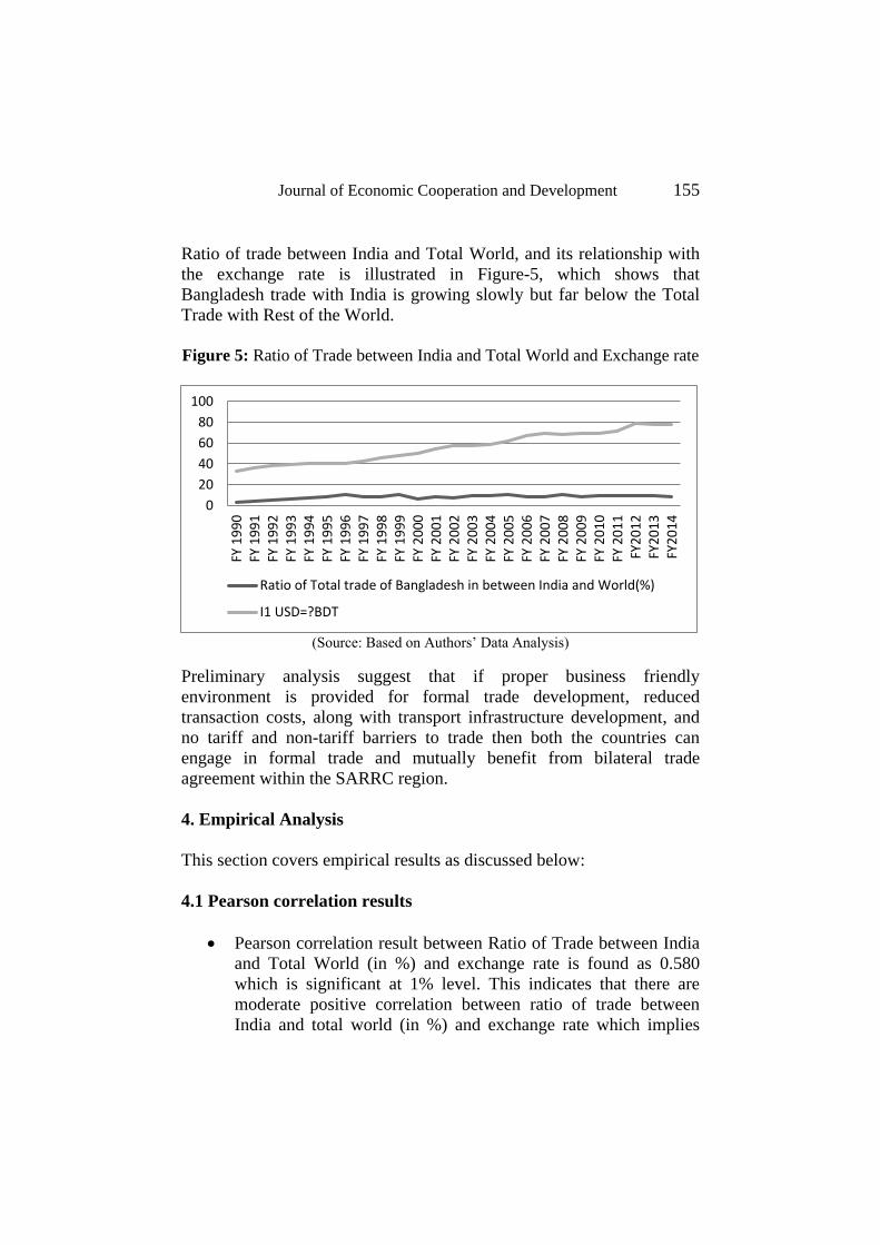
Journal of Economic Cooperation and Development 155
Ratio of trade between India and Total World, and its relationship with
the exchange rate is illustrated in Figure-5, which shows that
Bangladesh trade with India is growing slowly but far below the Total
Trade with Rest of the World.
Figure 5: Ratio of Trade between India and Total World and Exchange rate
(Source: Based on Authors’ Data Analysis)
Preliminary analysis suggest that if proper business friendly
environment is provided for formal trade development, reduced
transaction costs, along with transport infrastructure development, and
no tariff and non-tariff barriers to trade then both the countries can
engage in formal trade and mutually benefit from bilateral trade
agreement within the SARRC region.
4. Empirical Analysis
This section covers empirical results as discussed below:
4.1 Pearson correlation results
Pearson correlation result between Ratio of Trade between India
and Total World (in %) and exchange rate is found as 0.580
which is significant at 1% level. This indicates that there are
moderate positive correlation between ratio of trade between
India and total world (in %) and exchange rate which implies
0
20
40
60
80
100
FY 1
99
0FY
19
91
FY 1
99
2FY
19
93
FY 1
99
4FY
19
95
FY 1
99
6FY
19
97
FY 1
99
8FY
19
99
FY 2
00
0FY
20
01
FY 2
00
2FY
20
03
FY 2
00
4FY
20
05
FY 2
00
6FY
20
07
FY 2
00
8FY
20
09
FY 2
01
0FY
20
11
FY2
01
2FY
20
13
FY2
01
4
Ratio of Total trade of Bangladesh in between India and World(%)
I1 USD=?BDT
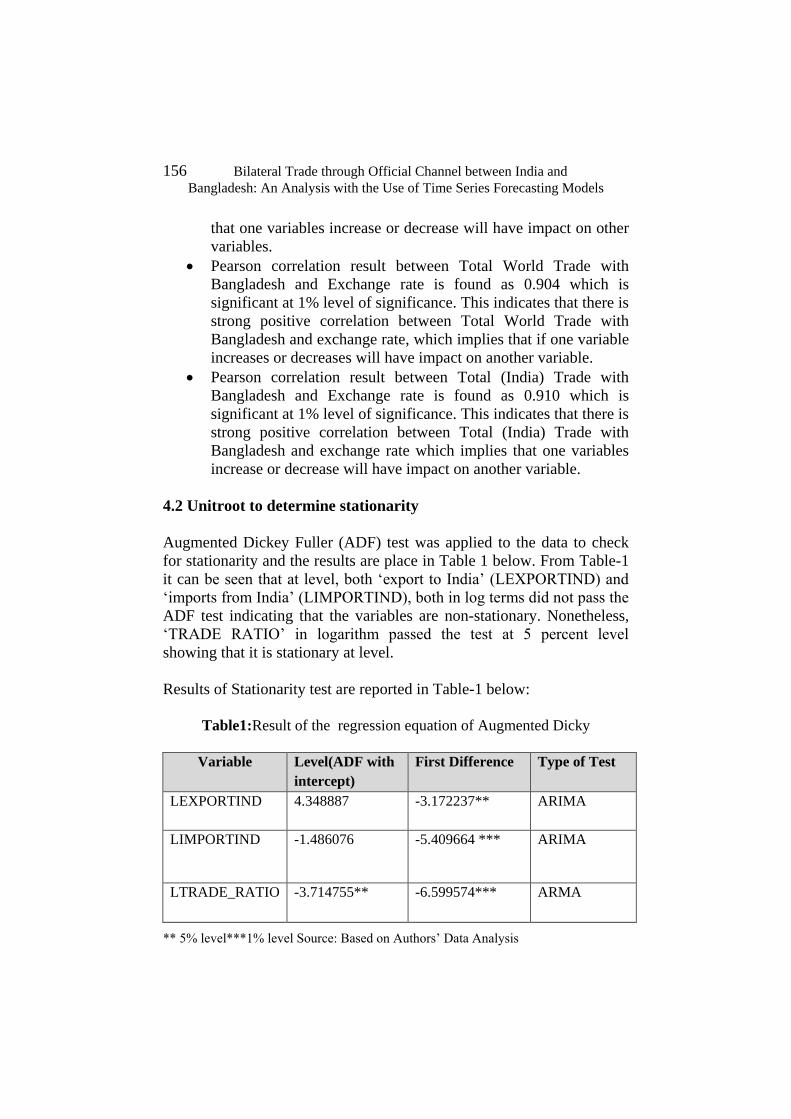
156 Bilateral Trade through Official Channel between India and
Bangladesh: An Analysis with the Use of Time Series Forecasting Models
that one variables increase or decrease will have impact on other
variables.
Pearson correlation result between Total World Trade with
Bangladesh and Exchange rate is found as 0.904 which is
significant at 1% level of significance. This indicates that there is
strong positive correlation between Total World Trade with
Bangladesh and exchange rate, which implies that if one variable
increases or decreases will have impact on another variable.
Pearson correlation result between Total (India) Trade with
Bangladesh and Exchange rate is found as 0.910 which is
significant at 1% level of significance. This indicates that there is
strong positive correlation between Total (India) Trade with
Bangladesh and exchange rate which implies that one variables
increase or decrease will have impact on another variable.
4.2 Unitroot to determine stationarity
Augmented Dickey Fuller (ADF) test was applied to the data to check
for stationarity and the results are place in Table 1 below. From Table-1
it can be seen that at level, both ‘export to India’ (LEXPORTIND) and
‘imports from India’ (LIMPORTIND), both in log terms did not pass the
ADF test indicating that the variables are non-stationary. Nonetheless,
‘TRADE RATIO’ in logarithm passed the test at 5 percent level
showing that it is stationary at level.
Results of Stationarity test are reported in Table-1 below:
Table1:Result of the regression equation of Augmented Dicky
Variable Level(ADF with
intercept)
First Difference Type of Test
LEXPORTIND 4.348887 -3.172237** ARIMA
LIMPORTIND -1.486076 -5.409664 ***
ARIMA
LTRADE_RATIO -3.714755**
-6.599574*** ARMA
** 5% level***1% level Source: Based on Authors’ Data Analysis

Journal of Economic Cooperation and Development 157
At first difference, both the variables could reject the null hypothesis of
unit root at 5 percent and 1 percent level respectively. This means that
the variables are stationary at first difference. Thereby, we may
conclude that both exports to India and imports from India variables are
integrated of order 1, i.e. I (1). From Table-1, we can observe that
Augmented Dicky Fuller Model’s intercept of LEXPRTIND and
LIMPORTTIND is not significant. As such the study will test ARIMA
model .But for the LTRADE -RATIO‘s Augmented Dicky Fuller
Model’s intercept is significant at 5% level for which we shall test
ARMA model. In Table-1 the stationarity test indicates that first
difference of export is negative but significant at 5% level. In case of
import it is negative, but significant at 1% level. In case of trade ratio
intercept is significant at 5% level, while first difference is significant at
1% level although the sign is negative. Of the several alternatives, the
best estimate for exports and imports with India is reported in Table-2,
showing the results of ARIMA Model- Exports to India. Further, details
related to Table-2 are given in appendix as Table: 1.
Table2: Results of ARIMA Model: Exports to India Sample 1990-2014
LEXPORTIND
=
2312 +0.5148
AR(3)
+0.4849
AR(5)
+1.2820
MA(1)
+0.9032
MA(2)
t-statistics 0.001 2.63 2.15 11.24 10.74
Adjusted R2= 0.9353 F= 58.78
Source: Based on Authors’ Data Analysis
Table-3, reports the results of ARIMA Model- Imports from India. It can
be seen that all the t-test results were acceptable with high adjusted R2
and F-statistics. The forecasting power of the model is good. The
predictive power of the model indicates that actual and predicted values
have high level of close match. Detail of Table-3 is given in appendix as
Table: 2.

158 Bilateral Trade through Official Channel between India and
Bangladesh: An Analysis with the Use of Time Series Forecasting Models
Table 3: Results of ARIMA Model: Imports from India - Sample 1990-
2014
LIMPORTI
ND
13.6 +0.9814AR
(1)
-0.9044MA
(1)
+0.5165MA
(2)
-0.5645MA
(4)
t-statistics 0.72 18.11 -5.03 3.36 -6.72
Adjusted R2= 0.9508 F =97.57
Source: Based on Authors’ Data Analysis
Table-4 below reports results of ARMA Model: Imports from India.
From the above Table-4, it can be observed that the equation adjusted
R2 is quite good and F statistics is acceptable, because as per ARMA
model it indicates that export to India is good as the equation-2 indicates
significant. But import and trade ratio indicates insignificant. Detail of
Table-4 is given in appendix as Table: 3.
Table 4: Results of ARMA Model: Trade Ratio - Sample 1990-2014
LTRADE_RATIO 2.13 +0.4509AR
(2)
-1.072MA
(1)
-1.1294MA
(2)
t-statistics 42.3 10.88 -2.45 -2.49
Adjusted R2= 0.7905 F =24.9
Source: Based on Authors’ Data Analysis
4.4 Forecast Evaluation
Table-5 evaluates the forecast results on exports and imports with India.
It reports the various measures of forecasting errors, viz., root mean
squared, mean absolute error, mean absolute percentage error, and Theil
coefficient.

Journal of Economic Cooperation and Development 159
Table 5: Forecast Evaluation
LEXPORTINDF LIMPORTINDF
Root Mean Squared Error 0.546811 0.204959
Mean Absolute Error 0.461016 0.171026
Mean Abs Percent Error 11.46903 2.505528
Theil Inequality Coefficient 0.057629 0.014459
Bias Proportion 0.710818 0.008751
Variance Proportion 0.045676 0.028413
Covariance proportion 0.243506 0.962836
Source: Based on Authors’ Data Analysis
It may be noted that our forecast is limited and it could not be extended
for out-of-sample, as number of the observation are made in only 14
years. From Table-5 it is discernible that the calculated value of RMSE
is almost of the same magnitude as that of MAE. They can be equal if
all errors are exactly the same. The smaller the reported errors, the better
will be the forecasting ability of the model. The Theil coefficient is also
less <1 one. It does not necessarily lead to acceptance of the model, but
does indicate that it performs better than other models.
From Table-5, it can be observed that imports from Bangladesh will be
relatively better if there is an increase in exports from Bangladesh to
India. Root Mean Squared Error is a measure of standard deviation
(SD). In case of exports SD is 0.546811 while for imports SD is
0.204959.Root Mean Squared Error for import is relatively better. Mean
absolute percentage error (MAPE), is determining prediction accuracy
of a forecasting method. As such MAPE for exports is 11.46903 while
MAPE for imports is 2.505528. Therefore, imports have a better
predictive accuracy. Theil inequality coefficient gives information about
accuracy of forecasting method for exports to India, which will be
0.057629, while in case of imports it will be 0.014459.It indicates that
imports from India are good for Bangladesh. Bias proportion which
indicates systematic error of 0.710818 is observed for exports to India,
while for imports is 0.008751.
160 Bilateral Trade through Official Channel between India and
Bangladesh: An Analysis with the Use of Time Series Forecasting Models
Bias indicated systematic error and as for import value is close to zero
so it is relatively better than export. In case of variance proportion,
which pointed out the capability of the forecasts to replicate degree of
variability in the variable to be forecast, we observed that for exports it
is 0.045676 while for imports it is 0.028413.As the variance proportion
of export is large then the import, so it means that actual series has
fluctuated considerably, whereas the forecast has not. Covariance
proportion which measures unsystematic error indicates that for exports
it is 0.243506 while for imports it is 0.972836. Covariance of imports is
higher than exports, so highest proportion of inequality is relatively
good. An overall result from aforesaid forecasting evaluation differs
from our previous findings in Table: 2, as Import is relatively better than
export in Table:5.
5. Conclusions, Implications and Future Research Directions
The study concludes that in the forecasting model, import is good for
Bangladesh. Bangladesh being a small economy is less competitive than
India, for which formal trade in terms of imports can create value chain
between the two countries. This is due to the fact that while importing
from the India being a neighbouring country, transportation costs are
low. On the other hand as per the ARIMA model, best fit equation is
exports to India. Bangladesh should put emphasis on exporting products
to India as per their demand at a completive price, as well as maintain
high quality of the product. Suranovic (2010) comments on creating
competitive market will lead to efficiency in bilateral trade for
Bangladesh. However, until today, quality of goods exported from
Bangladesh to India are not up to the standard and therefore, is not well
equipped to compete in the Indian market. Further, Hassan (2001)
asserts that the reason for Bangladesh’s low intra-regional trade within
the SAARC region is due to not producing goods that are demanded by
the SAARC countries, low level of industrialisation and diversification
of the industry. Hassan, Mehanna and Bashar (2001), also concluded
from their study that within the framework of SAARC regional block ,
South Asian Preferential trade opportunities should be explored for
economic cooperation, potential for trade liberalisation policies and
concessions to reap the gains from mutually beneficial trade. However,
due to the absence of complementarity in production, resource base,
financial limitations, political tensions, there is low volume of intra-
Journal of Economic Cooperation and Development 161
regional trade which can be mutually beneficial to the SAARC or
BIMSTEC countries.
If Bangladesh can export readymade high quality branded clothing to
the western world, then the questions is why the same quality is not
maintained for exports to India. Excellence in maintaining first world
quality and benchmarking for the standard of the products at
international level by Bangladesh, with low cost, may create competitive
advantage to sustain favourable bilateral trade position with India, which
will ultimately narrow down balance of trade position. Further,
Wangwe’s (1993) view regarding the role of government policy in
promoting competitiveness in the economy of Bangladesh, for creating
competiveness in the production process will assist to achieve
favourable trade situation in the future. However, social and political
stability, zero-tolerance to terrorism, and building trust between two
nations especially at the political leadership level is extremely
significant to manage mutual benefits from bi-lateral free trade
agreement (FTA).Srinivasan (2002) suggestions should be considered
by the policy makers so that efficiency and effectiveness as well as
competitiveness in the bilateral trade through official channel should be
improved, so that informal trade can be reduced. Trading through
official channel should to be free from bureaucratic delays and rent
seeking behaviour.
Formal trade between Bangladesh and India is forecasted to be
economically and mutually beneficial creating a win-win situation, if the
least cost combination is used to produce products, efficient
infrastructure and transportation system across border is provided,
business friendly environment, avoiding bureaucratic delay, red tape and
corruption is reduced, which can further ensure free trade and fair
pricing along with “partnership and cooperation” [see Singh (2014)]
for economic development. Krugman’s (1980) view should be
considered by the policy makers of Bangladesh as economies of scale
can be attained in the production process. Withdrawal of protection in
terms of trade barriers (tariff and non-tariff barriers) are not sufficient
for Bangladesh unless and until Bangladesh can earn competitiveness in
bilateral trade. Non-tariff measures are turned into non-tariff barriers by
India, while complying with sanitary and phyto-sanitary measures and
technical barriers to trade, which is not effective for enhancing trade.

162 Bilateral Trade through Official Channel between India and
Bangladesh: An Analysis with the Use of Time Series Forecasting Models
To reach sustainability in the long run through bilateral trade with India,
suppliers and manufacturer from Bangladesh ought to be concerned
about promoting development of world quality products, engage in
product differentiation, continuous innovation, attract new customers,
reliability of supply, investing and nurturing a sustainable business
enterprise through FTA.Indian foreign policy must also be business
friendly, towards gradually improving the bilateral trade relationship
which is supposed to be a combination of regional cooperation, as well
as meet the needs of the Indian market as also indicated by Ankit
(2015).Production intensity of Bangladesh in the industrial sector, both
export oriented industries and import substitution industries should be
raised. Thus, bilateral cooperation between the two countries will have
positive impact on creating economic efficiency and effectiveness. If
formal trade can be increased through efficient and effective services,
including infrastructural development, reducing transaction cost as
advocated by World Bank (2015), along with opportunities for cross-
border electricity trading [see Chattopadhyay and Fernando (2011)] will
not only result in rise in earnings from bilateral trade, but also meet the
increase in demand for power. However, India should withdraw tariff
and non-tariff barriers completely for SAPTA to work.
Given that Indian companies will have comparative advantage, mutually
agreed protective mechanisms can be put in place the transitional period,
for disadvantaged companies of Bangladesh. In the globalized regional
economy, India should give Bangladeshi exporters duty free access to
their market to a certain level, based on goods in demand. Innovative
and dynamic product lines, with assuring quality control of products
should be attained in Bangladesh in context of superior goods and
diversified exportable commodities should be produced by the country
to attain competitive advantage. Benchmarking of Bangladeshi product
with global standard should be obtained, as well as cost reduction and
establishing strategic alliances between both the country’s business
partners is required.
Bhagwati and Srinivasan (2002) advocated in their empirical findings
that globalization process is helpful for poor country. FTA between the
South Asian countries will be beneficial for which the platform of South
Asian Association of Regional Cooperation (SAARC) can be used, but
unfortunately it is not as successful as other regional trading agreements
such as ASEAN and EU. SAARC’s objective of economic cooperation

Journal of Economic Cooperation and Development 163
for promoting accelerated economic growth to improve the welfare and
quality of life of the people in South Asia has not been met. It is just a
cultural platform and not at all very effective in building trust and strong
business relationships in South Asia or having fruitful trade negotiations
under SAPTA. In order to build political, social, and economic ties to
mutually benefit the SAARC as well as BIMSTEC region, it is essential
to start first with building trust, disarm and focus on economic
development, outward looking economic policies to attract foreign
investment, improve institutions and promote growth through bilateral
preferential trade agreements. It seems that for India and Bangladesh
intra-regional trade is not as important, and they are more biased
towards trading with Rest of the World.
Current study is conducted based on secondary sources of trade data for
Bangladesh. For in-depth study, primary source can be used in future
research as to look at the informal trade between Bangladesh and its
bordering countries. Bilateral trade through official channel is beneficial
for both the countries and there is a wide scope to increase volume of
trade between the two countries through a collaborative approach,
private partnerships and capitalising on the huge potential benefit from
trade by providing business friendly environment, reduce informal trade
(smuggling) and transaction costs of doing business. It is thus essential
to build a sound foundation of trust, along with political wisdom to
eliminate all political conflicts and issues at all levels, in order to build
capacity, reap the benefits from economies of scale in trade flows,
attract direct investment from India in human and physical capital,
technology transfer, innovation and creation of economic efficiency ,for
which active cooperation, partnerships, and stability is required to
revitalize and rejuvenate the relationship between the two countries in
the 21st century.
164 Bilateral Trade through Official Channel between India and
Bangladesh: An Analysis with the Use of Time Series Forecasting Models
References
Acharya, L. and Marwaha, A. (2012), Status Paper on India-
Bangladesh Economic Relations, FICCI Report, December, pp.2-85.
Ahmed, I. (2006), “Bangladesh-India Relations: The context of SAARC
and the emerging global scenario,” Proceedings of a Conference, Asian
Affairs, 28 (2), 46-62.
Ahmed, K. A. (2015), “View from Bangladesh: Ten take-aways from
the Modi visit,” South Asian Free Media Association, June 10, 2015.
Alam, K.A., Uddin, M.G.S. and Alam, M.M., Malakar, B. (2009),
“Trade Patterns of Bangladesh with India and China: An Empirical
Evidence of the PPP Theory,” Journal of Regional Economic Studies, 2,
26-34.
Ankit, R. (2015), “In the Twilight of Empire: Two Impressions of
Britain and India at the United Nations, 1945-1947,”Journal of South
Asian Studies, Routledge, 30, 1-15.
Asteriou, D. and Hill, S. G. (2007),Applied Econometrics-A modern
Approach using Eviews and Microfit, Revised edition, Palgrave,
Macmillan, UK, 230-247.
Bammi, Y. M. (2010),India Bangladesh Relations: The Way Ahead, Vij
Books India Pvt Ltd., 51-54.
Basu, S. and Datta, D. (2007),“India-Bangladesh Trade Relations:
Problem of Bilateral Deficit,” Indian Economic Review, New Series,
42(1), 111-129.
Basher, Md. Abdul (2013),Indo-Bangla Trade: Composition, Trends and
Way Forward, Commonwealth Secretariat, April, 4-21.
Bhardwaj, S. (2014), An Agenda for the New Government: Policy
Options for India in Bangladesh, Institute of Peace and Conflict Studies,
IPCS issue brief no. 251, June.

Journal of Economic Cooperation and Development 165
Bhagwati, J. (1995), “Trade and Wages: Choosing among Alternative
Explanation,” Economic Policy Review, January, 42-47.
Bhagwati, J. and Srinivasan, T. N. (2002), “Trade and Poverty in the
Poor Countries,” The American Economic Review, 92(2), 180-183.
Bhuyan, A.R. (2006), “Bangladesh-India Trade Relations Prospects of a
Bilateral FTA,”Thoughts on Economics, 18(2),8-34.
Bown, C. P. (2014),Trade Policy Instruments over Time, Policy
Research Working Paper 6757, The World Bank, January, 2-23.
Chattopadhyay, D. and Fernando, P. N. (2011),“Cross-Border Power
Trading in South Asia: It’s Time to Raise The Game,”The Electricity
Journal, 10,1040-6190.
De, P. and Bhattacharyay, B. N. (2007),Prospects of India–Bangladesh
Economic Cooperation: Implications for South Asian Regional
Cooperation, ADB Institute Discussion Paper, No. 78, September, 1-36.
De, P., Raihan, S. and Kathuria, S. (2012),Unlocking Bangladesh-India
Trade Emerging Potential and the Way Forward, Policy Research
Working Paper, No 6155, The World Bank -South Asia Region
Economic Policy and Poverty Sector, August,1-33.
Dhaka Chamber of Commerce (2015),Viewed on 5th
July, 2015,
Available at:http://www.dhakachamber.com/home/saarc_trade: http:
//www.dhakachamber.com/home/saarc_trade.
Dutta, P. (2010),India-Bangladesh Relations issues, problems and recent
developments, Institute of Peace and Conflict Studies, IPCS Special
Report-97, September, 1-10.
Dutta, M. (1999), Economic regionalization in the Asia-Pacific:
challenges to economic cooperation, Edward Elgar Publishing, London.
Ethier, W. J. (2001), Regional Regionalism”, Regionalism and
Globalization-Theory and Practice, Lahiri, Sajal (Editor), Routledge,
London, 3-14.

166 Bilateral Trade through Official Channel between India and
Bangladesh: An Analysis with the Use of Time Series Forecasting Models
Gaurav, K., Bharti N. andSinha, P. (2015),ISFTA: Lessons for
Bangladesh, Chatterjee, S. Singh, N.P., Goyal , D.P., andGupta, N.
(Editors). Managing in Recovering Markets, Springer India, 351-367,
viewed on 5th July, 2015, Available at: http://www.dhakachamber.com
/home/saarc_trade.
Government of India. (2013), Foreign Relationship with Bangladesh, ,
Viewed on 2nd
November, 2015,Available at: http://www.mea.gov.
in/Portal/ForeignRelation/Bangladesh_Brief.pdf
Hassan, M. Kabir. (2001), “Is SAARC a Viable Economic Block?
Evidence from Gravity Model,” Journal of Asian Economics, 12, 263-
290.
Hassan, M. Kabir, Mehanna, Rock-Antoine, & Bashar, S. Abul. (2001),
Regional Cooperation in Trade, Finance and Investment among SAARC
Countries: The Bangladesh perspective, Draft November 25, 2001,
Viewed on 2nd
November, 2015, Available at: http://www.syedbasher.
org/published/2002_ToE.pdf.
Hassan, M. Kabir. (2002),“Trade With India and Trade Policies of
Bangladesh,” Chapter 10 in, Towards Greater Sub-Regional Economic
Cooperation: Limitations, Obstacles and Benefits, Edited by Forrest E.
Cookson and A.K.M. Shamsul Alam, University Press Limited (UPL),
Dhaka, Bangladesh, 2002: 349-401.
Hossain, A. and Rashid, S. (1999), “The Political Economy of
Bangladesh's Large and Growing Trade Deficits with India,” The
Pakistan Development Review, 38(1), 25-68.
Islam, M.M. (2011), “Trade cooperation between Bangladesh and India
with Special Reference to the North-East India,” Dialogue, April-June,
12(4).
Islam, R. M. G., Khan, M. T. andIshak, A. (2013), “Bilateral and
International Trade of Bangladesh and India: Effect of Falling Exchange
Rate of Indian Rupee,” European Journal of Business and Management,
5(27), 33-39.

Journal of Economic Cooperation and Development 167
Jain, S.C. (1999), “Prospects for a South Asian free trade agreement:
problems and challenges,” International Business Review, 8, 399-419.
Khan, S. M. (1999), “South Asian Association for Regional
Cooperation,” Journal of Asian Economics, 10, 489-495.
Khan, S. M. and Khan, Z. S. (2003),“Asian economic integration: a
perspective on South Asia,” Journal of Asian Economics, 13, 767-785.
Krugman, P. (1980), “Scale Economies, Product Differentiation, and the
Pattern of Trade,” The American Economic Review, 70(5), 950-959.
Mukherjee, D. (2015), India-Bangladesh: new trade links, Viewed on 6
July, 2015, Available at: http://www.fii-news.com/india-bangladesh-
trade-links/.
Pohit, S.and Taneja, N. (2003), “India's Informal Trade with
Bangladesh: A Qualitative Assessment,” World Economy, Blackwell
Publishing Ltd., 26(8), 1187-1214.
Pursell, G. andSattar, Z. (2006), India-Bangladesh Bilateral Trade and
Potential Free Trade Agreement, Bangladesh Development Series Paper
No: 13, The World Bank, World Bank Office, Dhaka Bangladesh, 4-5.
Rahman, M., Ahamad, M. G. Islam, A K M. and Amin, N. M.A.
(2012),Agricultural Trade between Bangladesh and India-An Analysis
of Trends, Trading Patterns and Determinants, CPD-CMI Working
Paper 3, Centre for Policy Dialogue, September, 1-42.
Rahman,M., Khan,A.R., Nabi, A., andPaul, T.K. (2010),Bangladesh’s
Export Opportunities in the Indian Market: Addressing Barriers and
Strategies for Future, CPD Working Paper Series,Paper-90,July,pp.1-26.
Rashid, HarunUr (2014), Bangladesh-India trade talks, The Daily Star,
March 26, Working Paper No. 232.
Rather, Z.A. and Gupta, D. (2014), “India-Bangladesh Bilateral Trade:
Problems and Prospects,” International Affairs and Global Strategy, 22,
42-48.
168 Bilateral Trade through Official Channel between India and
Bangladesh: An Analysis with the Use of Time Series Forecasting Models
Razzaque, M. A. and Basnett, Y. (2014), “Regional Integration in South
Asia: Trends, Challenges and Prospects,” Commonwealth Secretariat, 1-
17.
Sharma, R. (2015), Narendra Modi's $2 billion loan to Bangladesh, The
Independent, 10 June.
Sikdar, C. R. andChakraborty, M. (2006), “Bilateral Trade between
India and Bangladesh: A General Equilibrium Approach,”Economic
Systems Research, 18(3), 257-279.
Singh, N. (2014), “India and Development Partnership: Special
reference to Bangladesh in 21st century,”Elsevier -Procedia, Social and
Behavioral Science, 157,137-142.
Srinivasan, T.N. andVani, A. (2009),India in the Global and Regional
Trade: Determinants of Aggregate and Bilateral Trade Flows and Firms
Decision to Export, Indian Council for Research on International
Economic Relations, February Report, 1-22.
Srinivasan, T. N. (2002), Trade, Finance, and Investment in South
Asia,Berghahn Books, 164-165.
Suranovic, S. (2010), A Moderate Compromise: Economic Policy
Choice in an Era of Globalization, Palgrave McMillan, UK.
Sutherland, P. (2012), The Bilateral Free Trade, Project Syndicate.
Available at: http://www.project-syndicate.org/commentary/the-doha-
round-and-the-decline-of-the-world-trade-organization-by-peter-
sutherland.
The Indian Express (2015), NE trade bodies happy over PM Modi’s
Bangladesh trade pacts, June, 9, 2015.
Wangwe, S. (1993),New Trade Theories and Developing Countries:
Policy and Technological Implications, UNU/INTECH Working Paper
No. 7, June, 1-24.
Journal of Economic Cooperation and Development 169
World Bank (2006), India-Bangladesh Bilateral Trade and Potential Free
Trade Agreement, Bangladesh Development Series, Paper No: 13, The
World Bank Office, Dhaka, December, 1-87.
World Bank (2014), Economic Indicators, Viewed on 15th March, 2015,
Available at: http://data.worldbank.org/indicator/IC.BUS.EASE.XQ)
World Bank (2015), Informal and illegal trade: dimensions, trends,
composition, and the role of domestic indirect taxes, Chapter 8, 57-63,
viewed on 15th March, 2015, Available at: http://siteresources. worldbank
.org/SOUTHASIAEXT/Resources/223546-1168296540386/ch8.pdf.
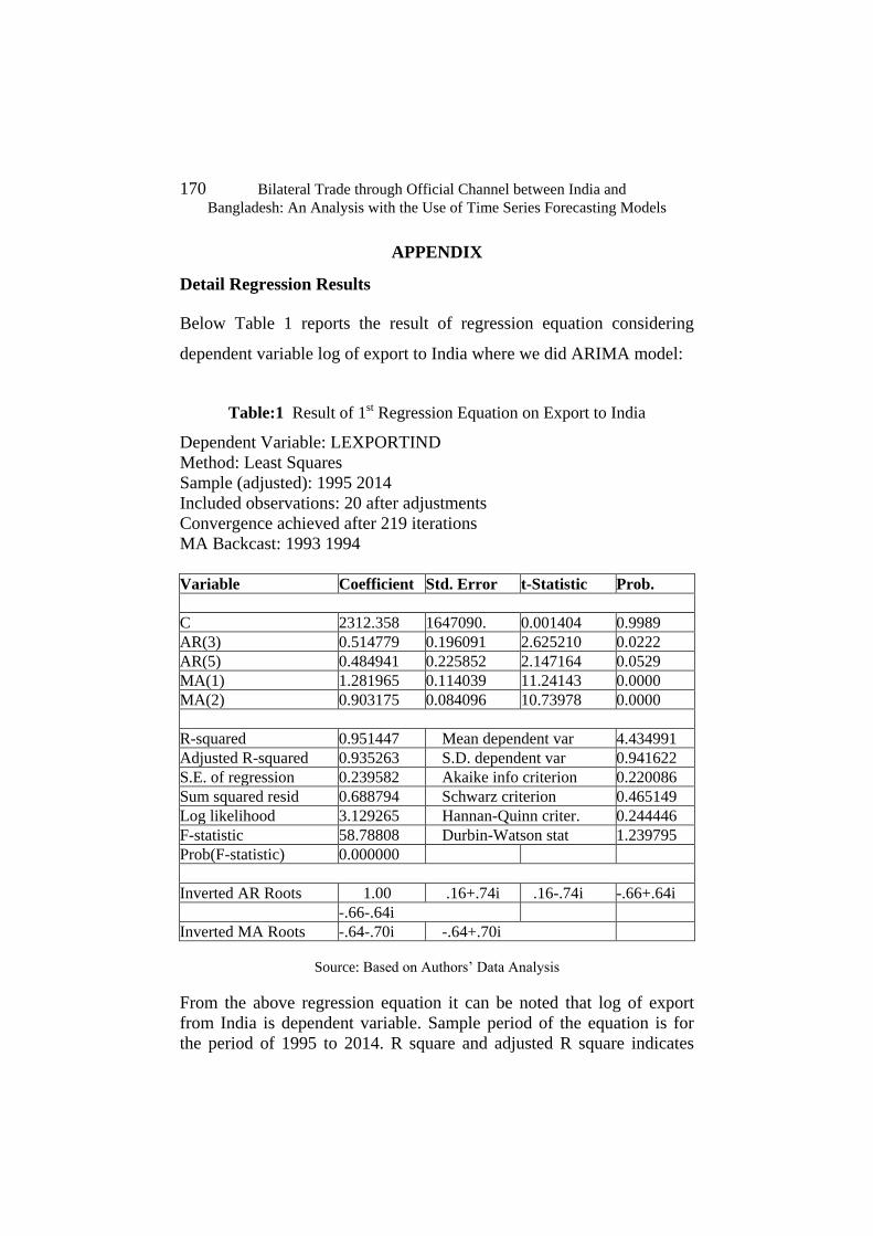
170 Bilateral Trade through Official Channel between India and
Bangladesh: An Analysis with the Use of Time Series Forecasting Models
APPENDIX
Detail Regression Results
Below Table 1 reports the result of regression equation considering
dependent variable log of export to India where we did ARIMA model:
Table:1 Result of 1st Regression Equation on Export to India
Dependent Variable: LEXPORTIND
Method: Least Squares
Sample (adjusted): 1995 2014
Included observations: 20 after adjustments
Convergence achieved after 219 iterations
MA Backcast: 1993 1994
Variable Coefficient Std. Error t-Statistic Prob.
C 2312.358 1647090. 0.001404 0.9989
AR(3) 0.514779 0.196091 2.625210 0.0222
AR(5) 0.484941 0.225852 2.147164 0.0529
MA(1) 1.281965 0.114039 11.24143 0.0000
MA(2) 0.903175 0.084096 10.73978 0.0000
R-squared 0.951447 Mean dependent var 4.434991
Adjusted R-squared 0.935263 S.D. dependent var 0.941622
S.E. of regression 0.239582 Akaike info criterion 0.220086
Sum squared resid 0.688794 Schwarz criterion 0.465149
Log likelihood 3.129265 Hannan-Quinn criter. 0.244446
F-statistic 58.78808 Durbin-Watson stat 1.239795
Prob(F-statistic) 0.000000
Inverted AR Roots 1.00 .16+.74i .16-.74i -.66+.64i
-.66-.64i
Inverted MA Roots -.64-.70i -.64+.70i
Source: Based on Authors’ Data Analysis
From the above regression equation it can be noted that log of export
from India is dependent variable. Sample period of the equation is for
the period of 1995 to 2014. R square and adjusted R square indicates

Journal of Economic Cooperation and Development 171
that the equation fits well. Autoregressive -3 is significant at 5% level of
significance. Autoregressive -5 is significant at 10% level of
significance. Moving average (1) and moving average (2) indicates
significance at 1% level of significance. Durbin Watson statistics
indicates autocorrelation; F statistics is significant at 1% level of
significance.
Below given Table - 2 reports the results of another regression equation
considering dependent variable as log of import to India where we did
ARIMA model:
Table:2- Result of Regression Equation on Import to India
Dependent Variable: LIMPORTIND
Method: Least Squares
Sample (adjusted): 1991 2014
Included observations: 24 after adjustments
Convergence achieved after 46 iterations
MA Backcast: 1987 1990
Variable Coefficient Std. Error t-Statistic Prob.
C 13.63823 18.75394 0.727219 0.4776
AR (1) 0.981427 0.054200 18.10737 0.0000
MA (1) 0.904408 0.179821 -5.029495 0.0001
MA (2) 0.516486 0.153668 3.361054 0.0040
MA (4) 0.564490 0.084048 -6.716257 0.0000
R-squared 0.960618 Mean dependent var 7.029149
Adjusted R-squared 0.950772 S.D. dependent var 0.869112
S.E. of regression 0.192833 Akaike info criter -0.249727
Sum squared resid 0.594953 Schwarz criterion -0.001032
Log likelihood 7.622137 Hannan-Quinn criter -0.195754
F-statistic 97.56833 Durbin-Watson stat 1.700202
Prob (F-statistic) 0.000000
Inverted AR Roots .98 .16+.74i .16-.74i -.66+.64i
Inverted MA Roots .98 .27+.9 .27-.92i -.62
Source: Based on Authors’ Data Analysis

172 Bilateral Trade through Official Channel between India and
Bangladesh: An Analysis with the Use of Time Series Forecasting Models
From the above regression equation it can be noted that log of imports
from India is dependent variable. Sample period of the equation is for
the period of 1991 to 2014. R square and adjusted R square indicates
that the equation fits well. Autoregressive -1 is significant at 1% level of
significance. Moving average (1), moving average (2), moving average
(4) indicates significance at 1% level of significance. Durbin Watson
statistics indicates no autocorrelation; F statistics is significant at 1%
level of significance. Table 3 below reports the result of regression
equation considering dependent variable as log of Trade ratio where we
did ARMA model:
Table:3 Result of the regression equation on Trade Ratio
Dependent Variable: LTRADE_RATIO
Method: Least Squares
Sample (adjusted): 1992 2014
Included observations: 23 after adjustments
Convergence achieved after 83 iterations
MA Backcast: OFF (Roots of MA process too large)
Variable Coefficient Std. Error t-Statistic Prob.
C 2.131033 0.050321 42.34847 0.0000
AR (2) 0.450850 0.041450 10.87699 0.0000
MA (1) -1.072187 0.437441 -2.451047 0.0261
MA (2) -1.129435 0.453246 -2.491880 0.0241
R-squared 0.823589 Mean dependent var 2.082005
Adjusted R-squared 0.790512 S.D. dependent var 0.188710
S.E. of regression 0.086372 Akaike info criter -1.883441
Sum squared resid 0.119363 Schwarz criterion -1.684295
Log likelihood 22.83441 Hannan-Quinn criter -1.844566
F-statistic 24.89910 Durbin-Watson stat 2.265035
Prob (F-statistic) 0.000003
Inverted AR Roots .67 -.67
Inverted MA Roots 1.73 -.65
Estimated MA process is noninvertible
Source: Based on Authors’ Data Analysis
Journal of Economic Cooperation and Development 173
From the Table: 3 regression equations it can be noted that log of trade
rate is dependent variable. Sample period of the equation is for the
period of 1992 to 2014. R square and adjusted R square indicates that
the equation fits well. Autoregressive -2 is significant at 1% level of
significance. Moving average (1), moving average (2), moving average
(4) indicates significance at 5% level of significance. Durbin Watson
statistics indicates that autocorrelation is significant at 1% level of
significance.


