Download - inventory,risk pooling

1
Inventory Management, Supply Contracts
and Risk Pooling

2
Inventory Management, Supply Contracts Inventory Management, Supply Contracts and Risk Poolingand Risk Pooling
Learning Objectives: Introduction to Inventory Management. The Effect of Demand Uncertainty:
Economic Order QuantityReorder PointsService levels (s,S) PolicyPeriodic Review PolicySupply ContractsRisk Pooling
Centralized vs. Decentralized Systems. Practical Issues in Inventory Management.

3
Types of Inventory & the Flow of MaterialsTypes of Inventory & the Flow of Materials
S
s
S
Supplier C
S
Supplier D
S
s
Supplier A
Supplier B
Work in Process
Finished Goods
Warehouse Y Warehouse Z
Customer Demand Customer Demand Customer Demand
Warehouse X

4
Role of Inventory in Supply ChainRole of Inventory in Supply Chain
Where do we hold inventory? Suppliers and manufacturers Warehouses and distribution centers Retailers
Types of Inventory WIP Raw materials Finished goods Distribution Inventories Maintenance, Repair, and Operational Suppliers (MROs) Transit Inventories
5
Role of Inventory in Supply ChainRole of Inventory in Supply Chain
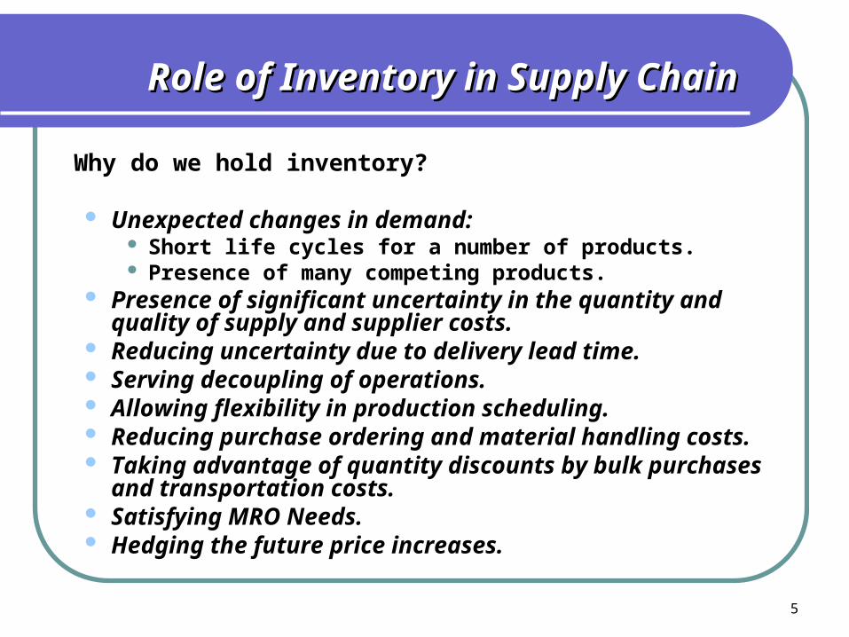
Why do we hold inventory?
Unexpected changes in demand: Short life cycles for a number of products. Presence of many competing products.
Presence of significant uncertainty in the quantity and quality of supply and supplier costs.
Reducing uncertainty due to delivery lead time. Serving decoupling of operations. Allowing flexibility in production scheduling. Reducing purchase ordering and material handling costs. Taking advantage of quantity discounts by bulk purchases
and transportation costs. Satisfying MRO Needs. Hedging the future price increases.

6
Role of Inventory in Supply ChainRole of Inventory in Supply Chain
By effectively managing inventory: Xerox eliminated $700 million inventory from its supply
chain. Wal-Mart became the largest retail company utilizing
efficient inventory management. GM has reduced parts inventory and transportation costs
by 26% annually. In 1984, GM’s distribution network consisted of:
20,000 Supplier plants. 133 Parts plants. 31 Assembly plants. 11, 000 dealers. Freight transportation costs were about US44.1 billion with 60% for
material shipments. Inventory valued at US$7.4 billion: 70% of this is WIP and the rest is
finished vehicles.

7
Role of Inventory in Supply ChainRole of Inventory in Supply Chain
By not managing inventory successfully:
In 1994, “IBM continues to struggle with shortages in their ThinkPad line” (WSJ, Oct 7, 1994).
In 1993, “Liz Claiborne said its unexpected earning decline is the consequence of higher than anticipated excess inventory” (WSJ, July 15, 1993).
In 1993, “Dell Computers predicts a loss; Stock plunges. Dell acknowledged that the company was sharply off in its forecast of demand, resulting in inventory write downs” (WSJ, August 1993).

8
Objectives of Inventory Management
Maximize customer service,
Maximize operational efficiency of the plant, and
Minimize investment in inventories.

9
Understanding InventoryUnderstanding Inventory
The inventory policy is affected by:
Demand Characteristics Replenishment Lead Time Number of Products Objectives
Service level Minimize costs
10
Inventory Cost StructureInventory Cost Structure
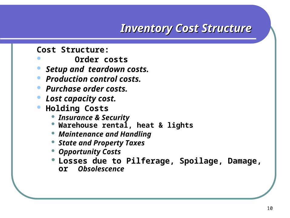
Cost Structure: Order costs Setup and teardown costs. Production control costs. Purchase order costs. Lost capacity cost. Holding Costs
Insurance & Security Warehouse rental, heat & lights Maintenance and Handling State and Property Taxes Opportunity Costs Losses due to Pilferage, Spoilage, Damage, or
Obsolescence

11
Economic Lot Size ModelEconomic Lot Size Model
Two major questions are of interest in formulating and solving the economic order quantity (EOQ) model.
How much should be ordered when the inventory for a given item is to be replenished?
When the order for a given item should be placed?
12
Economic Lot Size ModelEconomic Lot Size Model
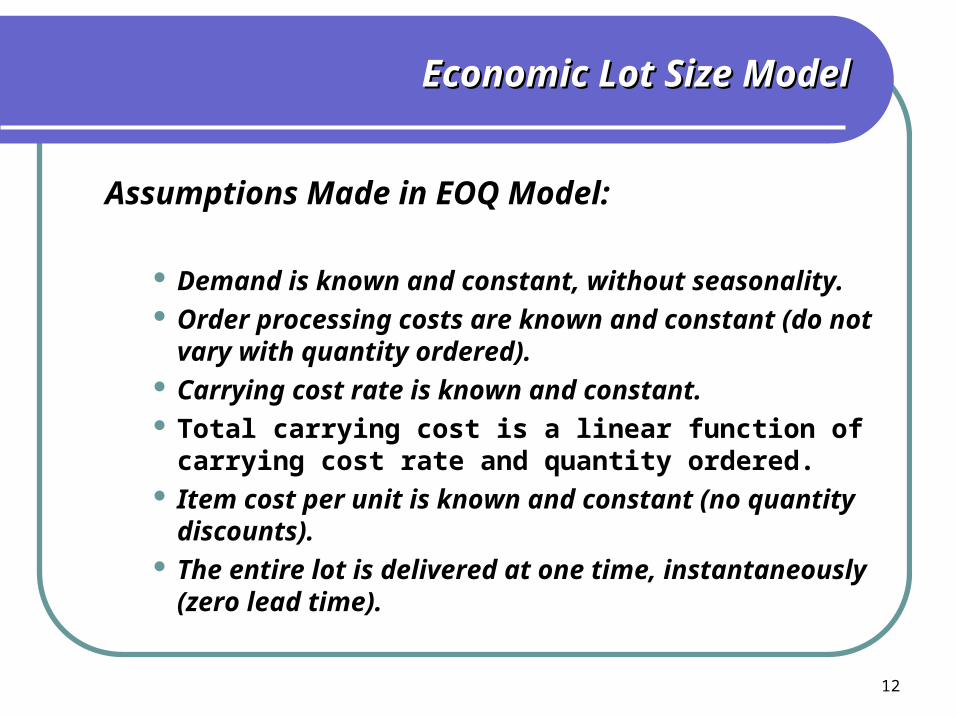
Assumptions Made in EOQ Model:
Demand is known and constant, without seasonality. Order processing costs are known and constant (do
not vary with quantity ordered). Carrying cost rate is known and constant. Total carrying cost is a linear function of carrying cost
rate and quantity ordered. Item cost per unit is known and constant (no quantity
discounts). The entire lot is delivered at one time, instantaneously
(zero lead time).

13
R = Reorder pointQ = Economic order quantityL = Lead time
L L
Q QQ
R
Time
Numberof unitson hand
1. You receive an order quantity Q.
2. Your start using them up over time. 3. When you reach down to
a level of inventory of R, you place your next Q sized order.
4. The cycle then repeats.

Cost Minimization Goal
Ordering Costs
HoldingCosts
Order Quantity (Q)
COST
Annual Cost ofItems (DC)
Total Cost
QOPT
By adding the item, holding, and ordering costs together, we determine the total cost curve, which in turn is used to find the Qopt inventory order point that minimizes total costs
By adding the item, holding, and ordering costs together, we determine the total cost curve, which in turn is used to find the Qopt inventory order point that minimizes total costs
Basic Fixed-Order Quantity (EOQ) Model Formula
H 2
Q + S
Q
D + DC = TC H
2
Q + S
Q
D + DC = TC
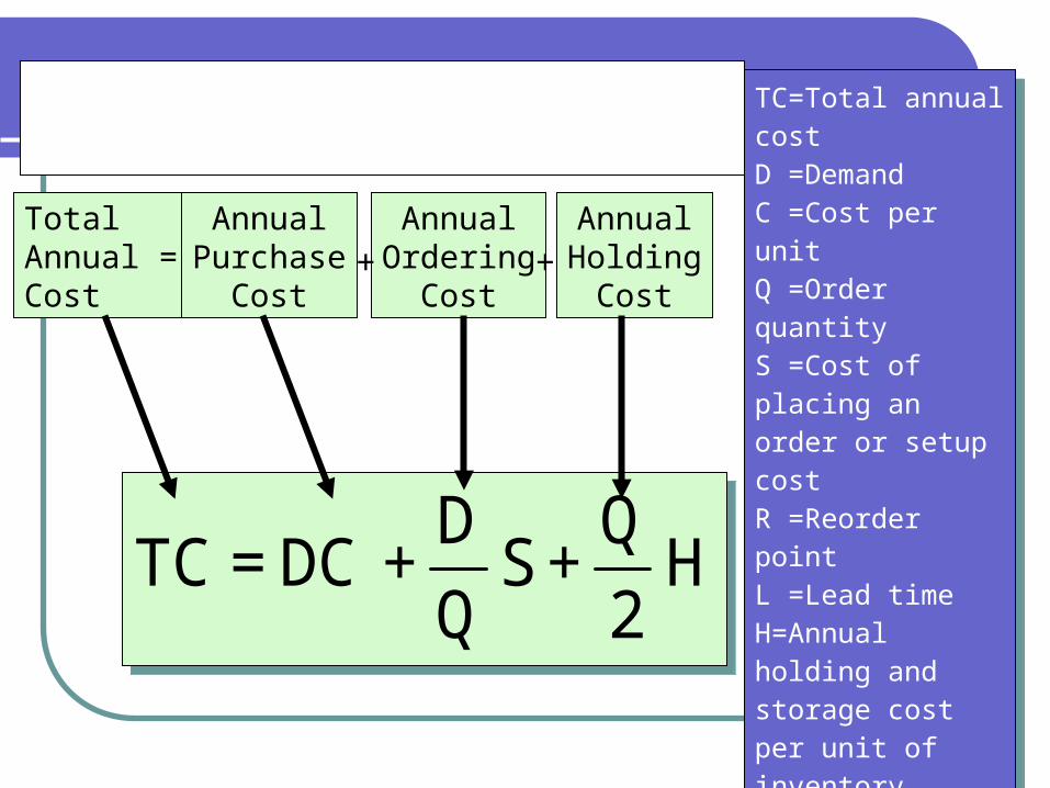
Total Annual =Cost
AnnualPurchase
Cost
AnnualOrdering
Cost
AnnualHolding
Cost+ +
TC=Total annual costD =DemandC =Cost per unitQ =Order quantityS =Cost of placing an order or setup costR =Reorder pointL =Lead timeH=Annual holding and storage cost per unit of inventory
TC=Total annual costD =DemandC =Cost per unitQ =Order quantityS =Cost of placing an order or setup costR =Reorder pointL =Lead timeH=Annual holding and storage cost per unit of inventory

Deriving the EOQ Using calculus, we take the first derivative of
the total cost function with respect to Q, and set the derivative (slope) equal to zero, solving for the optimized (cost minimized) value of Qopt
Using calculus, we take the first derivative of the total cost function with respect to Q, and set the derivative (slope) equal to zero, solving for the optimized (cost minimized) value of Qopt
Q = 2DS
H =
2(Annual D em and)(Order or Setup Cost)
Annual Holding CostOPTQ =
2DS
H =
2(Annual D em and)(Order or Setup Cost)
Annual Holding CostOPT
Reorder point, R = d L_
Reorder point, R = d L_
d = average daily demand (constant)
L = Lead time (constant)
_
We also need a reorder point to tell us when to place an order
We also need a reorder point to tell us when to place an order

EOQ Example (1) Problem Data
Annual Demand = 1,000 unitsDays per year considered in average
daily demand = 365Cost to place an order = $10Holding cost per unit per year = $2.50Lead time = 7 daysCost per unit = $15
Given the information below, what are the EOQ and reorder point?
Given the information below, what are the EOQ and reorder point?

EOQ Example (1) Solution
Q = 2DS
H =
2(1,000 )(10)
2.50 = 89.443 units or OPT 90 unitsQ =
2DS
H =
2(1,000 )(10)
2.50 = 89.443 units or OPT 90 units
d = 1,000 units / year
365 days / year = 2.74 units / dayd =
1,000 units / year
365 days / year = 2.74 units / day
Reorder point, R = d L = 2.74units / day (7days) = 19.18 or _
20 units Reorder point, R = d L = 2.74units / day (7days) = 19.18 or _
20 units
In summary, you place an optimal order of 90 units. In the course of using the units to meet demand, when you only have 20 units left, place the next order of 90 units.
In summary, you place an optimal order of 90 units. In the course of using the units to meet demand, when you only have 20 units left, place the next order of 90 units.

EOQ Example (2) Problem Data
Annual Demand = 10,000 unitsDays per year considered in average daily demand = 365Cost to place an order = $10Holding cost per unit per year = 10% of cost per unitLead time = 10 daysCost per unit = $15
Determine the economic order quantity and the reorder point given the following…
Determine the economic order quantity and the reorder point given the following…

EOQ Example (2) Solution
Q =2DS
H=
2(10,000 )(10)
1.50= 365.148 units, or OPT 366 unitsQ =
2DS
H=
2(10,000 )(10)
1.50= 365.148 units, or OPT 366 units
d =10,000 units / year
365 days / year= 27.397 units / dayd =
10,000 units / year
365 days / year= 27.397 units / day
R = d L = 27.397 units / day (10 days) = 273.97 or _
274 unitsR = d L = 27.397 units / day (10 days) = 273.97 or _
274 units
Place an order for 366 units. When in the course of using the inventory you are left with only 274 units, place the next order of 366 units.
Place an order for 366 units. When in the course of using the inventory you are left with only 274 units, place the next order of 366 units.

21
EOQ: Optimal Order QuantityEOQ: Optimal Order Quantity
Example: Suppose that an annual demand for an outdoor carpet is 20,000yds. The cost of placing an order is estimated at $50 per order, whereas the carrying cost rate per year is 20% and the item cost is $10. How many yards of outdoor carpet should be stocked?
D=20,000ydss=$50i=0.20c=10

22
EOQ Model: An ExampleEOQ Model: An Example
EOQ = Q* = 25020000/(0.2010)
= 1000 yds.

23
EOQ Model: An ExampleEOQ Model: An Example
The company must order 1000 yards when ever it orders. At this EOQ
Annual order processing costs =50(20000/ Q*) = 50(20000/1000) = $1000
Annual Carrying Costs=(0.2010)(Q*/2) = (0.2010)(1000/2) = $1000
24
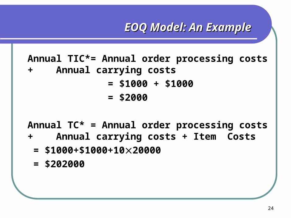
EOQ Model: An ExampleEOQ Model: An Example
Annual TIC*= Annual order processing costs + Annual carrying costs
= $1000 + $1000
= $2000
Annual TC* = Annual order processing costs + Annual carrying costs + Item Costs
= $1000+$1000+1020000
= $202000

25
The Effect of The Effect of Demand UncertaintyDemand Uncertainty
Most companies treat the world as if it were predictable: Production and inventory planning are based on
forecasts of demand made far in advance of the selling season.
Companies are aware of demand uncertainty when they create a forecast, but they design their planning process as if the forecast truly represents reality.
Recent technological advances have increased the level of demand uncertainty: Short product life cycles. Increasing product variety.

26
Demand ForecastDemand Forecast
The three principles of all forecasting techniques:
Forecasting is always wrong. The longer the forecast horizon the worst is the
forecast. Aggregate forecasts are more accurate.

27
SnowTime Sporting GoodsSnowTime Sporting Goods
Fashion items have short life cycles, high variety of competitors.
SnowTime Sporting Goods New designs are completed. One production opportunity. Based on past sales, knowledge of the industry, and
economic conditions, the marketing department has a probabilistic forecast.
The forecast averages about 13,100, but there is a chance that demand will be greater or less than this.

28
Supply Chain Time LinesSupply Chain Time Lines
Jan 00 Jan 01 Jan 02
Feb 00 Sep 00 Sep 01
Design Production Retailing
Feb 01Production

29
SnowTime Demand ScenariosSnowTime Demand Scenarios
Demand Scenarios
0%5%
10%15%20%25%30%
Sales
P
robability

30
SnowTime CostsSnowTime Costs
Production cost per unit (C): $80 Selling price per unit (S): $125 Salvage value* per unit (V): $20 Fixed production cost (F): $100,000 Q is production quantity, D demand
Profit =Revenue - Variable Cost - Fixed Cost + Salvage
*the amount expected to be realized upon the sale or other disposition of the asset when it is no longer useful to the program

31
SnowTime ScenariosSnowTime Scenarios
Scenario One: Suppose you make 12,000 jackets and demand
ends up being 13,000 jackets. Profit = 125(12,000) - 80(12,000) - 100,000 =
$440,000
Scenario Two: Suppose you make 12,000 jackets and demand
ends up being 11,000 jackets. Profit = 125(11,000) - 80(12,000) - 100,000 +
20(1000) = $ 335,000

32
SnowTime Best SolutionSnowTime Best Solution
Find the order quantity that maximizes the average profit.
Question: Will this quantity be less than, equal to, or greater than average demand?

33
What to Make?What to Make?
Question: Will this quantity be less than, equal to, or greater than average demand?
Average demand is 13,100.Look at marginal cost Vs. marginal profit
If a extra jacket sold during the season: Marginal profit = 125-80 = $45
If it is not sold during the season:Marginal cost = 80-20 = $60
So Snow Time should make less than average demand.
34
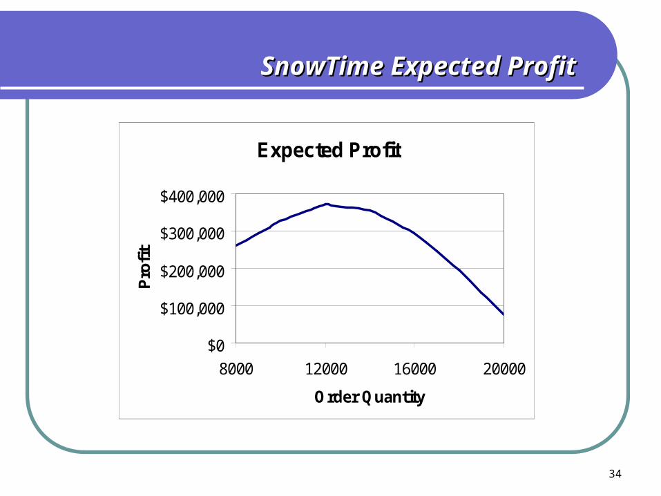
SnowTime Expected ProfitSnowTime Expected Profit
Expected Profit
$0
$100,000
$200,000
$300,000
$400,000
8000 12000 16000 20000
Order Quantity
Pro
fit

35
SnowTime Expected ProfitSnowTime Expected Profit
Expected Profit
$0
$100,000
$200,000
$300,000
$400,000
8000 12000 16000 20000
Order Quantity
Pro
fit

36
SnowTime: Important ObservationsSnowTime: Important Observations
Tradeoff between ordering enough to meet demand and ordering too much.
Several quantities have the same average profit. Average profit does not tell the whole story.

37
Key Insights From This ModelKey Insights From This Model
The optimal order quantity is not necessarily equal to average forecast demand.
The optimal quantity depends on the relationship between marginal profit and marginal cost.
As order quantity increases, average profit first increases and then decreases.
As production quantity increases, risk increases. In other words, the probability of large gains and of large losses increases.
38
Supply ContractsSupply Contracts
Buyers and suppliers usually agree on supply contracts. These contracts are very powerful tools that can used to ensure adequate supply and demand for goods.
In a supply contract the buyer and seller may agree on: Pricing and volume discounts. Minimum and maximum purchase quantities. Delivery lead times. Product or material quality. Product return policies.

39
Manufacturer Manufacturer DC Retail DC
Stores
Fixed Production Cost =$100,000
Variable Production Cost=$35
Selling Price=$125
Salvage Value=$20
Wholesale Price =$80
Supply ContractsSupply Contracts

40
Demand ScenariosDemand Scenarios
Demand Scenarios
0%5%
10%15%20%25%30%
Sales
P
roba
bilit
y

41
Retailer Expected ProfitRetailer Expected Profit
Expected Profit
0
100000
200000
300000
400000
500000
6000 8000 10000 12000 14000 16000 18000 20000
Order Quantity

42
Retailer Expected ProfitRetailer Expected Profit
Expected Profit
0
100000
200000
300000
400000
500000
6000 8000 10000 12000 14000 16000 18000 20000
Order Quantity

43
Supply Contracts (Cont.)Supply Contracts (Cont.)
Retailer optimal order quantity is 12,000 units. Retailer’s expected profit is $470,000 See the
Figure on previous slide). Manufacturer profit is $440,000 (= 12000(80-35)-
100000). Supply Chain Profit is $910,000 (470000+440000).
Is there anything that the retailer and manufacturer can do to increase the profit of both?

44
Supply Contracts (Cont’d)Supply Contracts (Cont’d)
Buy-Back Supply Contracts. Revenue-Sharing Contracts. Global Optimization. Quantity-Flexibility Contracts. Sales Rebate Contracts.

45
Manufacturer Manufacturer DC Retail DC
Stores
Fixed Production Cost =$100,000
Variable Production Cost=$35
Selling Price=$125
Salvage Value=$20
Wholesale Price =$80
Supply ContractsSupply Contracts

46
Retailer Profit Buy Back=$55)Retailer Profit Buy Back=$55)
Buy-Back Contracts:
Suppose the manufacturer offers to buy back unsold jackets from the retailer for $55.

47
Retailer Profit Buy Back=$55) Retailer Profit Buy Back=$55)
0
100,000
200,000
300,000
400,000
500,000
600,000
Order Quantity
Re
tail
er
Pro
fit

48
Retailer Profit (Buy Back=$55)Retailer Profit (Buy Back=$55)
0
100,000
200,000
300,000
400,000
500,000
600,000
6000
7000
8000
9000
1000
0
1100
0
1200
0
1300
0
1400
0
1500
0
1600
0
1700
0
1800
0
Order Quantity
Re
tail
er
Pro
fit
$513,800

49
Manufacturer Profit (Buy Back=$55)Manufacturer Profit (Buy Back=$55)
0
100,000
200,000
300,000
400,000
500,000
600,000
Production Quantity
Ma
nu
factu
rer
Pro
fit

50
Manufacturer Profit (Buy Back=$55)Manufacturer Profit (Buy Back=$55)
0
100,000
200,000
300,000
400,000
500,000
600,000
Production Quantity
Ma
nu
fact
ure
r P
rofi
t
$471,900
51
Buy-Back SC Profit (Buy back = 55)Buy-Back SC Profit (Buy back = 55)
Under buy back at $55:
Retailer’s profit = $513,800.
Manufacturer’s profit = $471,900.
SC profit = 513,800+471,900 = $985700.

52
Supply Contracts (Cont’d)Supply Contracts (Cont’d)
Revenue-Sharing Contracts:
In revenue-sharing contracts, buyer shares some of its revenue with the seller, in turn for a discount on the wholesale price.
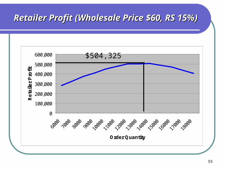
In this type a contract, manufacturer agrees to reduce the whole price from $80 to $60, and in return, the retailer provides 15% of the product revenue to the manufacturer.

53
Manufacturer Manufacturer DC Retail DC
Stores
Fixed Production Cost =$100,000
Variable Production Cost=$35
Selling Price=$125
Salvage Value=$20
Wholesale Price =$60
Supply ContractsSupply Contracts

54
Retailer Profit (Wholesale Price $60, RS Retailer Profit (Wholesale Price $60, RS 15%)15%)
0
100,000
200,000
300,000
400,000
500,000
600,000
Order Quantity
Re
tail
er
Pro
fit
55
Retailer Profit (Wholesale Price $60, RS Retailer Profit (Wholesale Price $60, RS 15%)15%)
0
100,000
200,000
300,000
400,000
500,000
600,000
Order Quantity
Re
tail
er
Pro
fit
$504,325

56
Manufacturer Profit (Wholesale Price $60, Manufacturer Profit (Wholesale Price $60, RS 15%)RS 15%)
0
100,000
200,000
300,000
400,000
500,000
600,000
700,000
Production Quantity
Ma
nu
fact
ure
r P
rofi
t

57
Manufacturer Profit (Wholesale Price $60, Manufacturer Profit (Wholesale Price $60, RS 15%)RS 15%)
0
100,000
200,000
300,000
400,000
500,000
600,000
700,000
Production Quantity
Ma
nu
fact
ure
r P
rofi
t
$481,375

58
Revenue-Sharing SC Profit (Wholesale Price Revenue-Sharing SC Profit (Wholesale Price $60, RS 15%)$60, RS 15%)
Under this RS Contract:
Retailer’s profit = $504,325.
Manufacturer’s profit = $481,375.
SC profit = 504,325+481,375 = $985,700.

59
Supply ContractsSupply Contracts
Strategy Retailer Manufacturer TotalSequential Optimization 470,700 440,000 910,700 Buyback 513,800 471,900 985,700 Revenue Sharing 504,325 481,375 985,700

60
Supply Contracts (Cont’d)Supply Contracts (Cont’d)
Global Optimization:
Both the manufacturer and the retailer are considered as two members of the same organization, causing the transfer of money between the two parties is ignored.
In this case, the supply chain marginal profit is $90=$125-$35, and the marginal loss is $15 = $35-$20.

61
Manufacturer Manufacturer DC Retail DC
Stores
Fixed Production Cost =$100,000
Variable Production Cost=$35
Selling Price=$125
Salvage Value=$20
Wholesale Price =$80
Supply ContractsSupply Contracts

62
Supply Chain ProfitSupply Chain Profit
0
200,000
400,000
600,000
800,000
1,000,000
1,200,000
Production Quantity
Su
pp
ly C
ha
in P
rofi
t

63
Supply Chain ProfitSupply Chain Profit
0
200,000
400,000
600,000
800,000
1,000,000
1,200,000
Production Quantity
Su
pp
ly C
ha
in P
rofi
t $1,014,500

64
Supply ContractsSupply Contracts
Strategy Retailer Manufacturer TotalSequential Optimization 470,700 440,000 910,700 Buyback 513,800 471,900 985,700 Revenue Sharing 504,325 481,375 985,700 Global Optimization 1,014,500

65
Supply Contracts: Key InsightsSupply Contracts: Key Insights
Effective supply contracts allow supply chain partners to replace sequential optimization by global optimization.
Buy Back and Revenue Sharing contracts achieve this objective through risk sharing.
66
Supply Contracts: Case StudySupply Contracts: Case Study
Example: Demand for a movie newly released video cassette typically starts high and decreases rapidly
Peak demand last about 10 weeks Blockbuster purchases a copy from a studio for
$65 and rent for $3 Hence, retailer must rent the tape at least 22 times
before earning profit Retailers cannot justify purchasing enough to
cover the peak demand In 1998, 20% of surveyed customers reported that
they could not rent the movie they wanted

67
Supply Contracts: Case StudySupply Contracts: Case Study
Starting in 1998 Blockbuster entered a revenue sharing agreement with the major studios
Studio charges $8 per copy Blockbuster pays 30-45% of its rental income
Even if Blockbuster keeps only half of the rental income, the breakeven point is 6 rental per copy
The impact of revenue sharing on Blockbuster was dramatic
Rentals increased by 75% in test markets Market share increased from 25% to 31% (The 2nd
largest retailer, Hollywood Entertainment Corp has 5% market share)

68
Other ContractsOther Contracts
Quantity Flexibility ContractsSupplier provides full refund for returned
items as long as the number of returns is no larger than a certain quantity
Sales Rebate ContractsSupplier provides direct incentive for the
retailer to increase sales by means of a rebate paid by the supplier for any item sold above a certain quantity
69
SnowTime Costs: Initial InventorySnowTime Costs: Initial Inventory
Production cost per unit (C): $80 Selling price per unit (S): $125 Salvage value per unit (V): $20 Fixed production cost (F): $100,000 Q is production quantity, D demand
Profit =Revenue - Variable Cost - Fixed Cost +
Salvage

70
SnowTime Expected ProfitSnowTime Expected Profit
Expected Profit
$0
$100,000
$200,000
$300,000
$400,000
8000 12000 16000 20000
Order Quantity
Pro
fit

71
Initial InventoryInitial Inventory
Suppose that one of the jacket designs is a model produced last year.
Some inventory is left from last year. Assume the same demand pattern as before If only old inventory is sold, no setup cost.
Question: If there are 7000 units remaining, what should SnowTime do? What should they do if there are 10,000 remaining?

72
(s, S) Policies(s, S) Policies
For some starting inventory levels, it is better to not start production.
If we start, we always produce to the same level. Thus, we use an (s,S) policy. If the inventory
level is below s, we produce up to S. s is the reorder point, and S is the order-up-to
level. The difference between the two levels is driven
by the fixed costs associated with ordering, transportation, or manufacturing.

73
Market Two
Risk PoolingRisk Pooling
Consider these two systems:
Supplier
Warehouse One
Warehouse Two
Market One
Market Two
Supplier Warehouse
Market One

74
Risk PoolingRisk Pooling
For the same service level, which system will require more inventory? Why?
For the same total inventory level, which system will have better service? Why?
What are the factors that affect these answers?

75
Risk Pooling:Risk Pooling:Important ObservationsImportant Observations
Centralizing inventory control reduces both safety stock and average inventory level for the same service level.
What other kinds of risk pooling will we see?

76
Risk Pooling:Risk Pooling:Types of Risk PoolingTypes of Risk Pooling
Risk Pooling Across Markets Risk Pooling Across Products Risk Pooling Across Time
Daily order up to quantity is: LTAVG + z AVG LT
10 1211 13 14 15
Demands
Orders

77
To Centralize Or Not To CentralizeTo Centralize Or Not To Centralize
What is the effect on:Safety stock?Service level?Overhead?Lead time?Transportation Costs?

78
Centralized Decision: Supplier
Warehouse
Retailers
Centralized SystemsCentralized Systems

79
Factors that Drive Reduction in InventoryFactors that Drive Reduction in Inventory
Top management emphasis on inventory reduction (19%).
Reduce the Number of SKUs in the warehouse (10%).
Improved forecasting (7%). Use of sophisticated inventory management
software (6%). Coordination among supply chain members
(6%). Others.

80
Factors that Drive Inventory Turns Factors that Drive Inventory Turns IncreaseIncrease
Better software for inventory management (16.2%).
Reduced lead time (15%). Improved forecasting (10.7%). Application of SCM principles (9.6%). More attention to inventory management (6.6%). Reduction in SKU (5.1%). Others.

81
End of the Session
Thank You


