Download - Introduction to Transcriptomics Analysis

INSTRUCTOR:Aureliano Bombarely
Department of BioscienceUniversita degli Studi di [email protected]
Introduction to Transcriptomics Analysis
Class 12 - Practice about Differential Gene Expression.

• Exercise 1: Differential expression with CummeRBund.
• Exercise 1.1: Data upload.
• Exercise 1.2: Data filtering.
• Exercise 1.3: Quality control.
• Exercise 1.4: Differential expression test
• Exercise 2: Differential expression with DESeq2.
• Exercise 2.1: Data upload.
• Exercise 2.2: Data filtering.
• Exercise 2.3: Differential expression test.
• Exercise 2.4: Quality control.
Outline of Topics

Data source

Data source
Col C24
Col x C24 C24 x Col

A- RNASeq Analysis pipeline with Hisat2-StringTie-Ballgown
Pertea, Mihaela, et al. "Transcript-level expression analysis of RNA-seq experiments with HISAT, StringTie and Ballgown." Nature protocols 11.9 (2016): 1650.

A- RNASeq Analysis pipeline with Hisat2-StringTie-Ballgown
Pertea, Mihaela, et al. "Transcript-level expression analysis of RNA-seq experiments with HISAT, StringTie and Ballgown." Nature protocols 11.9 (2016): 1650.

A- RNASeq Analysis pipeline with Hisat2-StringTie-Ballgown
https://rstudio-pubs-static.s3.amazonaws.com/289617_cb95459057764fdfb4c42b53c69c6d3f.html

• Exercise 1: Differential expression with CummeRBund.
Preparation before the exercise:
1- Transfer the Stringtie output from the server to your computer to work with R. To do it use Filezilla.

• Exercise 1: Differential expression with CummeRBund.
Preparation before the exercise:
2- Open RStudio
2.1- Load the Ballgown library: library(ballgown)as well as RColorBrewer, genefilter and dplyr
2.2- Set up as working directory the same one that contains the directories with the Stringtie results

• Exercise 1: Differential expression with CummeRBund.
Preparation before the exercise:
3- Prepare a tabular text file (PhenoData.txt) with the experimental design
Sample_id (same than the directory name)
Accession name
Experiment comparisons
Replicates

• Exercise 1: Differential expression with CummeRBund.
• Exercise 1.1: Data upload.
• Exercise 1.2: Data filtering.
• Exercise 1.3: Quality control.
• Exercise 1.4: Differential expression test
• Exercise 2: Differential expression with DESeq2.
• Exercise 2.1: Data upload.
• Exercise 2.2: Data filtering.
• Exercise 2.3: Differential expression test.
• Exercise 2.4: Quality control.
Outline of Topics
• Exercise 1: Differential expression with CummeRBund.
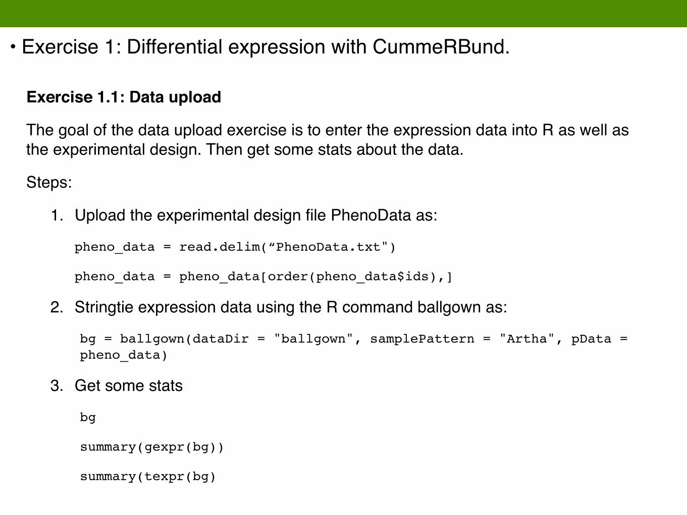
Exercise 1.1: Data upload
The goal of the data upload exercise is to enter the expression data into R as well as the experimental design. Then get some stats about the data.
Steps:
1. Upload the experimental design file PhenoData as:
pheno_data = read.delim(“PhenoData.txt")
pheno_data = pheno_data[order(pheno_data$ids),]
2. Stringtie expression data using the R command ballgown as:
bg = ballgown(dataDir = "ballgown", samplePattern = "Artha", pData = pheno_data)
3. Get some stats
bg
summary(gexpr(bg))
summary(texpr(bg)

• Exercise 1: Differential expression with CummeRBund.
• Exercise 1.1: Data upload.
• Exercise 1.2: Data filtering.
• Exercise 1.3: Quality control.
• Exercise 1.4: Differential expression test
• Exercise 2: Differential expression with DESeq2.
• Exercise 2.1: Data upload.
• Exercise 2.2: Data filtering.
• Exercise 2.3: Differential expression test.
• Exercise 2.4: Quality control.
Outline of Topics

• Exercise 1: Differential expression with CummeRBund.
Exercise 1.2: Data filtering
The goal of the data filtering exercise is to filter out the low expressed transcripts. It will also divide the experimental design by datasets.
Steps:
1. Select the transcript with expressions > 1 FPKM:
bg_filt = subset(bg,"rowVars(texpr(bg)) >1",genomesubset=TRUE)
2. Select the specific datasets for pure lines and hybrids:
bg_subset_PLN = subset(bg_filt, "type == 'pure_line'", genomesubset=FALSE)
bg_subset_HYB = subset(bg_filt, "type == 'hybrid'", genomesubset=FALSE)
3. Check the summary for the filtered data
bg_filt
summary(gexpr(bg_filt))
summary(texpr(bg_filt)
• Exercise 1: Differential expression with CummeRBund.
• Exercise 1.1: Data upload.
• Exercise 1.2: Data filtering.
• Exercise 1.3: Quality control.
• Exercise 1.4: Differential expression test
• Exercise 2: Differential expression with DESeq2.
• Exercise 2.1: Data upload.
• Exercise 2.2: Data filtering.
• Exercise 2.3: Differential expression test.
• Exercise 2.4: Quality control.
Outline of Topics

• Exercise 1: Differential expression with CummeRBund.
Exercise 1.3: Quality control
The goal of the quality control exercise is to visualise different parameters to assess the quality of the experiment.
Steps:
1. Library FPKM distribution
gene_expression = as.data.frame(gexpr(bg_filt))
colnames(gene_expression) = gsub("FPKM.", "", colnames(gene_expression))
data_colors = c("red1", "red2", "red3", "orange1", "orange2", "orange3", "salmon1", "salmon2", "salmon3", "green1", "green2", "green3")
short_names = gsub("ep", "", gsub("Artha_", "", colnames(gene_expression)))
boxplot(log2(gene_expression[,c(1:12)]+1), col=data_colors, names=short_names, las=2, ylab="log2(FPKM)", main="Distribution of FPKMs for all 12 libraries”, cex.axis=0.8)

• Exercise 1: Differential expression with CummeRBund.
Exercise 1.3: Quality control
The goal of the quality control exercise is to visualise different parameters to assess the quality of the experiment.
Steps:
1. Library FPKM distribution

• Exercise 1: Differential expression with CummeRBund.
Exercise 1.3: Quality control
The goal of the quality control exercise is to visualise different parameters to assess the quality of the experiment.
Steps:
2. Comparison of the expression between replicates
x = gene_expression[,”Artha_C24_Rep1”]
y = gene_expression[,”Artha_C24_Rep2”]
plot(x=log2(x+1), y=log2(y+1), pch=16, col="blue", cex=0.25, xlab=colnames(x), ylab=colnames(y), main="Comparison of expression values for a pair of replicates")
abline(a=0,b=1)
rs=cor(x,y)^2
legend("topleft", paste("R squared = ", round(rs, digits=3), sep=""), lwd=1, col="black")

• Exercise 1: Differential expression with CummeRBund.
Exercise 1.3: Quality control
The goal of the quality control exercise is to visualise different parameters to assess the quality of the experiment.
Steps:
2. Comparison of the expression between replicates
Low correlation
value
Create a matrix with all the samples
Why?

• Exercise 1: Differential expression with CummeRBund.
Exercise 1.3: Quality control
The goal of the quality control exercise is to visualise different parameters to assess the quality of the experiment.
Steps:
2. Comparison of the expression between replicatescorrelation_matrix = data.frame(matrix(vector(), nrow=12, ncol=12))colnames(correlation_matrix) = colnames(gene_expression)row.names(correlation_matrix) = colnames(gene_expression)i_n = 0for (i in colnames(gene_expression)) { i_n = i_n + 1 j_n = 0 for (j in colnames(gene_expression)) { j_n = j_n + 1 x = gene_expression[,i] y = gene_expression[,j] rs=cor(x,y)^2 correlation_matrix[i_n, j_n] = rs }}heatmap(as.matrix(correlation_matrix))

• Exercise 1: Differential expression with CummeRBund.
Exercise 1.3: Quality control
The goal of the quality control exercise is to visualise different parameters to assess the quality of the experiment.
Steps:
2. Comparison of the expression between replicates
Wrong sample name assignment
Wrong upload labels
at NCBI
Samples of 90 bp cluster together

• Exercise 1: Differential expression with CummeRBund.
Exercise 1.3: Quality control
The goal of the quality control exercise is to visualise different parameters to assess the quality of the experiment.
Steps:
3. MDS distance plot
d = 1 - correlation_matrix
mds=cmdscale(d, k=2, eig=TRUE)
par(mfrow=c(1,1))
plot(mds$points, type="n", xlab="", ylab="", main="MDS distance plot (all non-zero genes) for all libraries", xlim=c(-0.5,0.6), ylim=c(-0.5,0.5))
points(mds$points[,1], mds$points[,2], col="grey", cex=2, pch=16)
text(mds$points[,1], mds$points[,2], short_names, col=data_colors)

• Exercise 1: Differential expression with CummeRBund.
Exercise 1.3: Quality control
The goal of the quality control exercise is to visualise different parameters to assess the quality of the experiment.
Steps:
3. MDS distance plot

• Exercise 1: Differential expression with CummeRBund.
Exercise 1.3: Quality control
Can we fix the problem?
Comparison with the tables from the publication
• Exercise 1: Differential expression with CummeRBund.
• Exercise 1.1: Data upload.
• Exercise 1.2: Data filtering.
• Exercise 1.3: Quality control.
• Exercise 1.4: Differential expression test
• Exercise 2: Differential expression with DESeq2.
• Exercise 2.1: Data upload.
• Exercise 2.2: Data filtering.
• Exercise 2.3: Differential expression test.
• Exercise 2.4: Quality control.
Outline of Topics

• Exercise 1: Differential expression with CummeRBund.
Exercise 1.4: Differential expression test
The goal of the differential expression test is to run a statistical test on the expression data to test if each of the genes/transcripts have a statistically different expression.
When the test is run, it is essential to have a clear idea of the conditions that are compared. Most of the statistical tools produce a pairwise comparison.
The steps are:
1. Perform the statistical test selecting the two conditions to compare. In this case we will compare “pure_lines” vs “hybrids”.
results_genes = stattest(bg_filt, feature="gene", covariate="type", getFC=TRUE, meas="FPKM")
2. Add gene names to the output table.bg_table = texpr(bg_filt, 'all')
bg_gene_names = unique(bg_table[, 9:10])
results_genes = merge(results_genes, bg_gene_names, by.x=c(“id"), by.y=c("gene_id"))

• Exercise 1: Differential expression with CummeRBund.
Exercise 1.4: Differential expression test
The goal of the differential expression test is to run a statistical test on the expression data to test if each of the genes/transcripts have a statistically different expression.
When the test is run, it is essential to have a clear idea of the conditions that are compared. Most of the statistical tools produce a pairwise comparison.
The steps are:
3. Retrieve the significative genes (p-value < 0.05).sig=which(results_genes$pval<0.05)
length(sig)
4. Plot the results.results_genes[,"de"] = log2(results_genes[,"fc"])hist(results_genes[sig,"de"], breaks=50, col="seagreen", xlim=c(-3, 3), xlab="log2(Fold change) Pure Lines vs Hybrids", main="Distribution of differential expression values")abline(v=-1, col="black", lwd=2, lty=2)abline(v=1, col="black", lwd=2, lty=2)legend("topleft", "Fold-change > 2", lwd=2, lty=2)

• Exercise 1: Differential expression with CummeRBund.
Exercise 1.4: Differential expression test
The goal of the differential expression test is to run a statistical test on the expression data to test if each of the genes/transcripts have a statistically different expression.
When the test is run, it is essential to have a clear idea of the conditions that are compared. Most of the statistical tools produce a pairwise comparison.
The steps are:
5. Generate a table with the results.ge_table = as.data.frame(gexpr(bg_filt))
ge_table$id = row.names(ge_table)
ge_table$MEAN_C24 = apply(ge_table[c("FPKM.Artha_C24_Rep1", "FPKM.Artha_C24_Rep2", "FPKM.Artha_C24_Rep3")], 1, mean)
ge_table$SD_C24 = apply(ge_table[c("FPKM.Artha_C24_Rep1", "FPKM.Artha_C24_Rep2", "FPKM.Artha_C24_Rep3")], 1, sd)
ge_table$MEAN_Col = apply(ge_table[c("FPKM.Artha_Col_Rep1", "FPKM.Artha_Col_Rep2", "FPKM.Artha_Col_Rep3")], 1, mean)
ge_table$SD_Col = apply(ge_table[c("FPKM.Artha_Col_Rep1", "FPKM.Artha_Col_Rep2", "FPKM.Artha_Col_Rep3")], 1, sd)

• Exercise 1: Differential expression with CummeRBund.
Exercise 1.4: Differential expression test
The goal of the differential expression test is to run a statistical test on the expression data to test if each of the genes/transcripts have a statistically different expression.
When the test is run, it is essential to have a clear idea of the conditions that are compared. Most of the statistical tools produce a pairwise comparison.
The steps are:
5. Generate a table with the results.
ge_table$MEAN_C24xCol = apply(ge_table[c("FPKM.Artha_C24xCol_Rep1", "FPKM.Artha_C24xCol_Rep2", "FPKM.Artha_C24xCol_Rep3")], 1, mean)
ge_table$SD_C24xCol = apply(ge_table[c("FPKM.Artha_C24xCol_Rep1", "FPKM.Artha_C24xCol_Rep2", "FPKM.Artha_C24xCol_Rep3")], 1, sd) ge_table$MEAN_ColxC24 = apply(ge_table[c("FPKM.Artha_ColXC24_Rep1", "FPKM.Artha_ColXC24_Rep2", "FPKM.Artha_ColXC24_Rep3")], 1, mean)
ge_table$SD_ColxC24 = apply(ge_table[c("FPKM.Artha_ColXC24_Rep1", "FPKM.Artha_ColXC24_Rep2", "FPKM.Artha_ColXC24_Rep3")], 1, sd)
ge_table = merge(ge_table, results_genes, by.y=“id")
write.csv(ge_table, “GE_TABLE.STRINGTIE_BG.csv”, row.names = FALSE)

• Exercise 1: Differential expression with CummeRBund.
• Exercise 1.1: Data upload.
• Exercise 1.2: Data filtering.
• Exercise 1.3: Quality control.
• Exercise 1.4: Differential expression test
• Exercise 2: Differential expression with DESeq2.
• Exercise 2.1: Data upload.
• Exercise 2.2: Data filtering.
• Exercise 2.3: Differential expression test.
• Exercise 2.4: Quality control.
Outline of Topics

B- RNASeq Analysis pipeline with STAR-HTSeqCount—DESeq2
Processed Reads (FASTQ)
Mapped Reads (Sorted BAM)
Counted Reads (COUNTS)
DEGs (table)
STAR
HTSEQ-COUNT
DESEQ2
Indexed reference genomeReference Genome (FASTA)
Reference Annotation (GFF)

B- RNASeq Analysis pipeline with STAR-HTSeqCount—DESeq2
http://bioconductor.org/packages/devel/bioc/vignettes/DESeq2/inst/doc/DESeq2.html

• Exercise 2: Differential expression with DESeq2
Preparation before the exercise:
1- Transfer the HTSeq-Count output from the server to your computer to work with R. To do it use Filezilla.

• Exercise 2: Differential expression with DESeq2
Preparation before the exercise:
2- Call the DESeq2 library and prepare the sampleTable object:
library(“DESeq2”)
setwd(<My_HTSeqCount_DESeq_directory>)
sampleFiles = grep("Artha",list.files("."),value=TRUE)
sampleCondition = c("Pure_line", "Pure_line", "Pure_line", "Hybrid", "Hybrid", "Hybrid", "Hybrid", "Hybrid", "Hybrid", "Pure_line", "Pure_line", "Pure_line")
sampleName = gsub("_HTSeqCount.counts", "", gsub("Artha_", "", sampleFiles))
sampleTable = data.frame(sampleName = sampleName, fileName = sampleFiles, condition = sampleCondition)
sampleTable$condition = factor(sampleTable$condition)

• Exercise 1: Differential expression with CummeRBund.
• Exercise 1.1: Data upload.
• Exercise 1.2: Data filtering.
• Exercise 1.3: Quality control.
• Exercise 1.4: Differential expression test
• Exercise 2: Differential expression with DESeq2.
• Exercise 2.1: Data upload.
• Exercise 2.2: Data filtering.
• Exercise 2.3: Differential expression test.
• Exercise 2.4: Quality control.
Outline of Topics

• Exercise 2: Differential expression with DESeq2
Exercise 2.1: Data upload
The goal of the data upload exercise is to enter the count data into R as well as the experimental design. Then get some stats about the data.
Steps:
1. Upload the count data using the sampleTable as the experimental design:
ddsHTSeq = DESeqDataSetFromHTSeqCount(sampleTable = sampleTable, directory = ".", design= ~ condition)
2. Get some stats
ddsHTSeq
summary(counts(ddsHTSeq))

• Exercise 1: Differential expression with CummeRBund.
• Exercise 1.1: Data upload.
• Exercise 1.2: Data filtering.
• Exercise 1.3: Quality control.
• Exercise 1.4: Differential expression test
• Exercise 2: Differential expression with DESeq2.
• Exercise 2.1: Data upload.
• Exercise 2.2: Data filtering.
• Exercise 2.3: Differential expression test.
• Exercise 2.4: Quality control.
Outline of Topics

• Exercise 2: Differential expression with DESeq2
Exercise 2.2: Data filtering
The goal of the data filtering exercise is to filter out the low expressed transcripts (with less than 10 reads).
Steps:
1. Select the transcript with sum or counts > 10:
keep = rowSums(counts(ddsHTSeq)) >= 10
ddsHTSeq = ddsHTSeq[keep,]
2. Check the summary for the filtered data
ddsHTSeq
summary(counts(ddsHTSeq))

• Exercise 1: Differential expression with CummeRBund.
• Exercise 1.1: Data upload.
• Exercise 1.2: Data filtering.
• Exercise 1.3: Quality control.
• Exercise 1.4: Differential expression test
• Exercise 2: Differential expression with DESeq2.
• Exercise 2.1: Data upload.
• Exercise 2.2: Data filtering.
• Exercise 2.3: Differential expression test.
• Exercise 2.4: Quality control.
Outline of Topics

• Exercise 2: Differential expression with DESeq2
Exercise 2.3: Differential expression test
The goal is to perform the differential expression test on the samples.
Steps:
1. Run DESeq on the dds object and get the results:
ddsHTSeq = DESeq(ddsHTSeq)
res = results(ddsHTSeq)
2. Check the results
table(res$pvalue <= 0.05)
summary(res)

• Exercise 1: Differential expression with CummeRBund.
• Exercise 1.1: Data upload.
• Exercise 1.2: Data filtering.
• Exercise 1.3: Quality control.
• Exercise 1.4: Differential expression test
• Exercise 2: Differential expression with DESeq2.
• Exercise 2.1: Data upload.
• Exercise 2.2: Data filtering.
• Exercise 2.3: Differential expression test.
• Exercise 2.4: Quality control.
Outline of Topics

• Exercise 2: Differential expression with DESeq2
Exercise 2.4: Quality control.
There are several ways to perform a quality control for a DESeq analysis..
Steps:
1. Generate a MA-Plot:
plotMA(res, ylim=c(-2,2))

• Exercise 2: Differential expression with DESeq2
Exercise 2.4: Quality control.
There are several ways to perform a quality control for a DESeq analysis..
Steps:
2. Check counts for the lowest p-value feature:
plotCounts(ddsHTSeq, gene=which.min(res$pvalue), intgroup="condition")

• Exercise 2: Differential expression with DESeq2
Exercise 2.4: Quality control.
There are several ways to perform a quality control for a DESeq analysis..
Steps:
3. Heatmap of sample to sample distances: vsd = vst(ddsHTSeq, blind=FALSE)
sampleDists = dist(t(assay(vsd)))
library(“RColorBrewer”, “pheatmap")
sampleDistMatrix = as.matrix(sampleDists)
rownames(sampleDistMatrix) = names(vsd$sizeFactor)
colnames(sampleDistMatrix) = NULL
colors <- colorRampPalette( rev(brewer.pal(9, "Blues")) )(255)
pheatmap(sampleDistMatrix,
clustering_distance_rows=sampleDists,
clustering_distance_cols=sampleDists,
col=colors)

• Exercise 2: Differential expression with DESeq2
Exercise 2.4: Quality control.
There are several ways to perform a quality control for a DESeq analysis..
Steps:


