
1
Information Cascades in Multi-Agent Models
Arthur De Vany
Cassey Lee
University of California,
Irvine, CA 92697
1. Introduction
A growing literature has brought to our attention the importance of information
transmission and aggregation for economic and political behavior. If agents are
informationally decentralized and act on the basis of what is going on around them, their
local interactions may lead to very rich macro dynamics. How likely is it that an
economy with learning agents would converge on common beliefs? And how closely
would those beliefs match the underlying beliefs of the agents themselves? In systems of
decentralized, locally connected agents, how may information be inferred from the
actions of others? And, how important is the aggregation of information about group
behavior in guiding individual choices?
Many recent studies of cascades point to the possibility of information cascades in
economies with local learning and information transmission. Early models were known
by different terms---bandwagons, herding, and path-dependent choice. In each of these
cases, the choices of agents who act first inform and influence the choices of later agents.
In turn, these choices influence later agents and a time sequence of choice results. In this
sort of sequential decision process, if agents draw strong inferences from the choices of
others, they may make choices that are ex post non-optimal under full information. A
necessary ingredient in generating such a process is some form of bounded rationality;

2
agents cannot possess full information and foresight or they would have no need to draw
inferences from the actions of other agents.
Information cascades are defined as conformity that ignores one’s own tastes. As
Bickhchandani, Hirshleifter and Welch (1992) define it, an information cascade is a
sequence of decisions where it is optimal for agents to ignore their own preferences and
imitate the choice of the agent or agents ahead of them. Models of cascades answer two
key questions: Can they occur and are they fragile? In this paper, we examine both of
these questions and add a third: What sorts of distributions of choices do information
cascades produce? This is a natural question to ask because the dynamics of cascades
must have certain statistical properties. If the cascade “locks onto” a choice among
several, as the theory posits, then the resulting distribution of choices must be skewed and
highly uneven. If information cascades are fragile, then they should exhibit “large”
fluctuations and they may have complex basins of attraction. Both of these questions
come down to the same one: What are the properties of the statistical distributions to
which information cascades converge?
A weakness of the literature on information cascades is the lack of empirical
research. Do the models make correct predictions? Are they testable? Are they capable
of explaining observed behavior? At the present, the evidence is only anecdotal and
suggestive. Much needs to be done before information cascades can be accepted as real
explanations for observed data. The movies offer the opportunity to test information
cascade models. A movie is released to theaters in its opening week. Movie fans have
access to various sources of information---public and private. They are able to see how
many people are choosing each movie by reading the newspaper, watching the evening
3
news, or through trade publications and sources on the Internet. Thus, they are able to
observe signals about the actions of other agents in the manner assumed in cascade
models. In fact, one could argue that the studios’ casting, marketing, and release
strategies are an attempt to initiate a cascade. Because movies play out their run over
time, one can observe the dynamics of box office attendance and revenues for evidence
of cascades and convergence in distribution.
A number of papers have characterized motion picture revenue dynamics (see
below) and have modeled the effect of the dynamics on the distribution of revenues.
These papers raise some doubts that information cascade models are capable of
explaining the data. Cascade models give a reasonable account of the skewed
distribution of revenues that one finds in the movies, but they fail to account for certain
important features of the dynamics. In addition, cascade models make rather strong
claims about the frequency of information cascades (they are virtually assured to happen)
and their optimality (they are as easily wrong as right). We think that cascade models go
wrong in their failure to incorporate information about quality. In the prevailing models,
agents observe only the actions of others and must infer the quality of products from
these actions. Hence, an agent can only imitate but not learn from the actions of others.
So, our first task is to extend the information available to agents beyond actions to
include the quality experienced by others.
The second place where cascade models go wrong in our opinion is the way they
structure agent interactions. Agents make decisions sequentially as though they are
standing in a line and they observe the actions of all the other agents ahead of them in the
line. Hence, the information structure is global and there is no local interaction of the

4
sort that agent-based modeling regards as fundamental. So, our second task is to put
some structure on the way information is transmitted among agents and to see how that
affects the dynamics and outcomes of cascades.
Our model extends the basic model of the information cascade in these ways:
First, the sources of information include local observation of actions and a summary
statistic about choices in the aggregate. Second, there are many choices, not just two as
in most other models of information cascades. Consequently, we are modeling a
competition among cascades. Third, there is the possibility to choose none of the
alternatives. This model contains the basic model, which can be recovered by varying
the parameters that weight the signal sources and number of alternative choices. One
would expect these expanded information sources and choices to diminish the possibility
that a cascade will sweep one of the choices to dominance.
The purpose, then, of this paper is to investigate the properties of information
cascades and the statistical distribution of choices they generate within the context of the
motion picture industry. This grounds the analysis in the evidence and lets us examine
the kinds of information dynamics that could account for “hits” and “bombs” in the
movies, a subject that is intriguing in its own right. We use multi-agent models to
simulate the distribution of agents across movies. The model incorporates both local and
global interactions. Agents choose sequentially and interact with their immediate
predecessors, by observing their actions or receiving a message from them about a
movie's quality. In addition, agents have access to global information about the market
shares of movies in a way that closely mimics the reports on the evening news. There

5
has been concern that reporting the grosses of the top movies has encouraged herding and
made movies worse and our model can shed some light on this issue.
The outline for the rest of the paper is as follows. Section 2 surveys the related
literature briefly. In section 3, a version of Bikhchandani, Hirshleifer and Welch's (1992)
action-based model is simulated. This model is extended to a quality- and quantity-based
model in section 4. The dynamics of competition among good and bad movies and the
influence of the opening week are examined in section 5. Section 6 concludes.
2. Literature
A seminal paper by Bikhchandani et al (1992) explains the conformity and
fragility of mass behavior in terms of informational cascades. In a closely related paper
Banerjee (1992) models optimizing agents who engage in herd behavior which results in
an inefficient equilibrium. Anderson and Holt (1997) are able to induce information
cascades in a laboratory setting by implementing a version of Bikhchandani et al's (1992)
model.
The second strand of literature examines the relationship between information
cascades and large fluctuations. Lee (1998) shows how failures in information
aggregation in a security market under sequential trading result in market volatility. Lee
advances the notion of “informational avalanches” which occurs when hidden
information (e.g. quality) is revealed during an informational cascade thus reversing the
direction of information cascades.
The third strand explores the link between information cascades and heavy tailed
distributions. Cont and Bouchaud (1998) put forward a model with random groups of

6
imitators that gives rise to stock price variations that are heavy-tailed distributed. De
Vany and Walls (1996) use a Bose-Einstein allocation model to model the box office
revenue distribution in the motion picture industry. The authors describe how supply
adapts dynamically to an evolving demand that is driven by an information cascade (via
word-of-mouth) and show that the distribution converges to a Pareto-Lévy distribution.
The ability of the Bose-Einstein allocation model to generate the Pareto size distribution
of rank and revenue has been proven by Hill (1974) and Chen (1978). De Vany and
Walls (1996) present empirical evidence that the size distribution of box office revenues
is Pareto. Subsequent work by Walls (1997), De Vany and Walls (1999a), and Lee
(1999) has verified this finding for other markets, periods and larger data sets. De Vany
and Walls (1999a) show that the tail weight parameter of the Pareto-Levy distribution
implies that the second moment may not be finite. Lastly, De Vany and Walls (1999b)
have shown that motion picture information cascades begin as action-based, non-
informative cascades, but undergo a transition to an informative cascade after enough
people have seen it to exchange “word of mouth” information. At the point of transition
from an uninformed to an informed cascade, there is loss of correlation and an onset of
turbulence, followed by a recovery of week to week correlation among high quality
movies.
3. The BHW Model of Action-Based Information Cascades
Bikhchandani, Hirshleifer and Welch (1992) model information cascades as
imitative decision processes. In their model, Bayesian agents choose to adopt or reject an
action based on their own private information and information about the actions of all the

7
other agents who chose before them. The agents are essentially in a line, the order of
which is exogenously fixed and known to all, and they are able to observe the binary
actions (adopt or do not adopt) of all the agents ahead of them. The agents infer the
signal of the other agents in the sequence from their actions: the agent reasons that if an
agent adopts, then they must have gotten a high signal. If enough agents adopt, then the
agent may ignore her own signal because the weight of the evidence of previous
adoptions overcomes the weight the agent places on her own signal. Thus, according to
the model, a rational agent may ignore her own information and imitate the choices of
agents who choose before her.
Key results of their paper include:
1. As the precision of the private signal of the value of adoption increases, a correct
cascade (the agent adopts when the true value warrants adoption) starts with higher
probability and earlier.
2. If the signal is noisy enough the probability of an incorrect cascade can be as high as
0.5.
3. An agent with high precision choosing early can start a cascade, but the high-precision
agent can also shatter a cascade if he chooses later.
4. The probability that no cascade occurs is decreasing in the number of agents in the
sequence.
5. An increase in the number of agents increases the probability that a cascade starts.
6. A cascade once started will last forever.
7. The release of a small amount of public information can shatter a long-lasting cascade.

8
8. As the number of public information releases increases, the correct choice becomes
clearer and individuals settle into the correct cascade.
We develop an agent-based version of the Bikchandani, Hirshleifer, and Welch
model (1992, henceforth BHW) of an information cascade. We have several objectives
in what follows. We examine the properties of simulated information cascades and
compare them to the theoretical predictions of the BHW model. Since cascade models
are not analytically closed and their dynamics are stochastic and complex, it is not clear
what their time paths and attractors look like and how sensitive these are to different
parameterizations. In their article, BHW give probabilities that cascades will occur but
the paper contains no explicit dynamics. This is a gap we want to fill.
It appears that the reason the BHW model may be analyzed solely through its ex
ante probabilities is that the asymptotics of the model are so strong that the probabilities
reach their limits within 3 to 5 agents. And this is true no matter how accurate the private
signals are. Consequently, the information cascade settles to its attractor in a few moves.
This seems to us to be too strong a result and suggests that almost any string of choices
will become a cascade in which agents ignore their own information and preferences.
In Figure 1 we plot BHW’s ex ante probability that a cascade will not occur as a
function of the signal accuracy and the number of agents in the choice sequence. As is
evident, the probability that there is no cascade is small for all values of the accuracy of
the prior probability and number of agents (N) and quickly goes to zero as the length of
the choice sequence grows. Values of N as low as 3 and 5 are sufficient for a cascade to
be almost certain to occur. Virtually all choice sequences longer than 3 or 4 become
cascades, no matter how accurate private signals are. Consequently, the concept of a

9
cascade becomes almost vacuous since virtually any sequence of more than 4 choices
will almost surely be a cascade. Because it converges so rapidly, the BHW model does
not determine how probabilities evolve endogenously with the actual choices made along
the choice sequence. This is an issue we seek to address.
But, there is a deeper problem---the problem of identifying a cascade in a
sequence of choices. The BHW model predicts the probabilities that cascades will occur.
This means that the results apply to a large sample of choice sequences, not to any
particular sequence. The model says that, in a large sample of choice sequences, the
frequency of (long) paths that are not cascades will be vanishingly small. Any single
choice path may display segments of UP or DOWN cascades or NO cascade. That means
one must observe a large number of sequences to see if the process generating them is an
information cascade in the BHW sense. A single choice sequence is not sufficient to
identify an information cascade.
We explicitly incorporate local and global communication among agents. Some
models of information cascades assume information is aggregated---in the BHW model,
the agents can see all the way down the line to observe all the choices made ahead of
them. Others assume agents only see a few of the choices made before them---this is a
strictly local form of information. We explicitly model the local and aggregate
information available to agents to assess their relative contributions to cascades. In
addition, we extend the model beyond the binary choice model to include choices among
many alternatives.
Can the extended model give an account of the known empirical features of the
box office revenue dynamics of motion pictures? Because motion picture audiences

10
choose sequentially and use both local (word of mouth) and global (box office reports)
information, it is a dynamical process that offers a nice test of cascade models and of the
nature of their dependence on information structure. Can information cascades produce
the skewed, heavy-tailed distributions that are found in motion pictures?
3.1. An Agent-Based Model of Information Cascades
In the BHW model agents choose sequentially between adopting or rejecting a single
product. Each individual privately observes a conditionally independent signal X about
the value of the product. Individual i's signal Xi can be either High or Low. A signal
High is observed with probability p > 0.5 when the true value is High and a signal High is
observed with probability 1 – p when the true value is Low. Each agent in the choice
sequence observes the choices of all the agents ahead of them and uses this information
to infer the signal of the preceding agent. If a preceding agent chooses the product, the
next agent infers her signal was High; if the agent does not choose the product, she infers
the agent’s signal was Low.
In our model, agents choose between m products, which we will hereafter call
movies (though they could be software applications, clothing, stocks, or what have you).
They have access to two sources of information: they can observe the action of their
nearest neighbor and they can observe an aggregate signal. In this case, the nearest
neighbor is the agent who chose just before them. In addition, the agents have access to
the market shares of the products. The market shares of the products summarize the
choices of the agents who went before. As in BHW, the agent’s signal precision is a

11
probability p > 0.5 that the signal High will be observed when the true value is High and
1 – p when the true value is Low.
Assume that agent i sees movie j (i.e. i’s signal Xi = High). Agent i+1 will infer
agent i’s private signal Xij about movie j from i’s decision. If the second agent gets a
High signal (Xi+1=High), the agent will see movie j. Otherwise, Agent i+1 will flip a
coin to choose movie j or to see the movie with the highest market share.
If the previous agent chose no movie, the next agent will choose not to see a
movie if the agent's private signal is Low, or flip a coin to choose not to see a movie or to
see the movie with highest market share when the agent's signal is high. The choice logic
is diagrammed in Figure 2.
3.2. Signal Accuracy and Information Cascades
This model is simulated with 2,000 agents who are sequentially allocated among
20 movies. Before the simulation begins, each movie is given one agent. Then the first
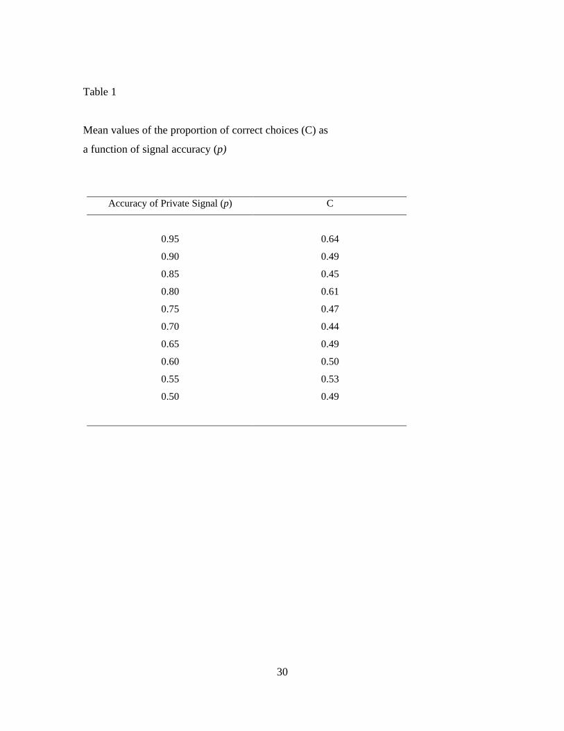
agent is allocated randomly to one of the 20 movies and the choice logic sets in. The
second agent observes the prior agent’s choice. We carry out twenty simulation runs for
each value of p from 0.5 to 0.9 with an increment of 0.05. A correct choice is defined as
one in which a good quality movie is chosen. In our simulation, half of the movies are
good movies and half are bad movies, though the agents are unable to communicate this
information and only observe the action of their immediate predecessor. The mean
numbers of correct choices over each sequence are tabulated for p in Table 1.
In the BHW model the probability of a correct cascade is increasing in the
accuracy of the private signals. The statistics of our simulation results in Table 1 cannot

12
confirm this result. A higher value of p is not necessarily associated with a higher mean
value of correct choices. The problem seems to be that a high p gives too much
credibility to the choice of the agent ahead and, thus, may steer the agents following onto
an inferior movie.
The BHW model also implies that the probability of a cascade is almost surely
one (the probability of no cascade is vanishing for N > 5 for any value of p, see Figure 1).
The simulations indicate that, at low values of p, cascades seldom occur and when they
do they are extremely fragile. As an example, consider Figures 3 (a) and 3 (b) which
depict movie choices over time for two extreme cases: p = 0.55 (low accuracy) and p =
0.95 (high accuracy).
In the figures, time evolves from left to right, each time step corresponding to a
decision. The vertical axis corresponds to the 20 movies. When a movie is selected that
is indicated by a dot at its vertical location. In the high accuracy case, the choices move
along a path at movie 10. But, there are sequences in which the same movie is chosen are
interrupted by jumps to other movies. The intermittent jumps don’t persist and the agents
eventually return to a cascade on movie 10 because it has the highest market share. It is
the global information that pulls the audience back to movie 10 after it jumps to other
movies. The random element in choice, and local information about the agent just ahead
in the sequence, are capable of moving a cascade away from the leading movie
temporarily, but the global information (market shares) eventually pulls it back if the
shares are sufficiently uneven. This highlights how important the global view posited in
standard models is to their results (recall each agent sees all the choices before she makes
hers).

13
When signal accuracy is low, the choice sequences jump randomly among movies
and the figure is typical of nearly all the simulations. There is no rapid convergence to a
cascade with the number of decisions, in contrast to the BHW model’s prediction. In
fact, there are no cascades when signals are below a threshold of accuracy. When signals
have high accuracy, information cascades do appear but they are fragile---they break and
then reappear---and the lengths of cascades correspond to “bursts” that appear to have a
power law distribution.
3.3. Information Cascades and the Distribution of Choices
In virtually all models of information cascades the agents choose among just two
alternatives. When choice is binary, an uneven distribution will mean that one alternative
gains all, or nearly all, of the market. When there are many possible choices, will
cascade-type choice processes also lock onto just one of the alternatives? Or will the
cascades jump back and forth between products so much that the distribution will be
fairly even?
This is an important question in the movie business, where cascades are thought
to be an important influence on the distribution of box office revenues. Indeed, studio
marketing is virtually built on the premise that cascades can be started with the right
campaign and stars. What is the nature of the box office distribution? A number of
studies show that the distribution of motion picture box office revenues is well fitted by a
Pareto-Lévy (stable) distribution with infinite variance. These distributions are “heavy
tailed” and have more probability mass on extreme outcomes than a normal distribution
(which is the only member of the class of stable distributions with finite variance). A

14
standard approach when dealing with such distributions is to examine their upper tail,
typically the top 10 percent, where they are power laws and to estimate a measure of
weight in the upper tail. The value of the weight in the tail is related to the so-called tail
index α.
Following a conventional approach, we estimate the tail index by applying least
squares regression to the upper ten percent of the observations generated by the
simulations. In this upper tail, a Lévy stable distribution is asymptotically a Pareto
distribution of the following form:
P[X > x] ~ x-α, for x > k (1)
where x is the number of agents allocated to each movie and k is “large”. A low value of
the tail index α corresponds to a slow decay of the tail and, hence, to what is called a
heavy tail.
In the following exercise we are interested in discovering what the distribution of
choices looks like. We also want to see if information cascade models are capable of
generating outcomes similar to the empirical findings. We allocate 2,000 agents to 200
movies via our agent-based version of the BHW model. This large number of movies is
required to give the degrees of freedom required to estimate the value of α from only the
top 10 percent of movies. For each value of p, we run twenty simulations. The statistics
of our simulations are in Table 2.
Our simulation results indicate that higher values of signal accuracy p are
associated with heavier-tailed distributions of agents over movies (i.e. lower α). This

15
result appears to be stronger for higher values of p - consistent with earlier simulation
results that show that informational cascades are less fragile for higher values of p. The
α estimates have a lower standard deviation at high values of p, which further supports
this view. Hence, there is a positive relationship between informational cascades and
heavy-tailed distributions, provided that signal accuracy p is sufficiently high.
A value of p of 0.7 gives a value of α of 1.5 that is virtually the same as the value
found in De Vany and Walls (1997, 1999a), Lee (1999), Walls (1997) and Sornette
(1999) for the movies. This consensus regarding the value of α can be considered to be
fairly reliable as the aforementioned studies cover different samples, countries, and time
frames, yet they all find a value of α close to 1.5.
It is known that the variance is infinite when the value of α is less than 2 and that
the mean is infinite when α is less than 1. As the results reported in the table indicate, at
a signal accuracy of 0.7 and higher, the second moment of the distribution is infinite and,
at accuracy 0.9, even the mean is infinite. The model is capable of generating Lévy -
stable distributions with the right value of α. The signal cannot be too noisy or the
distribution will be too flat and it cannot be too accurate or the distribution will be too
skewed.
The implications of finding that information cascades can produce heavy-tailed
distributions are a bit startling. If the variance and even the mean may not be finite, the
implication is that it is not possible to predict where the cascade will go in situations
where it is capable of capturing the dynamics of choice in a real situation. It indicates
that none of the conclusions derived from cascade models hold when there are several
choices and when a choice of none of the available alternatives is possible. Only when

16
signal accuracy is low is it possible to predict the mean with a finite variance and, in this
case, the distribution is essentially uniform. These are pretty negative assessments of the
predictive content of information cascade models.
4. A Model of Action- and Quality-Based Information Cascades
In the BHW model, the agents are not informed as to the quality of their choice
alternatives. They receive a private signal about quality but observe only the actions and
not the quality evaluations of the agents who precede them in the sequence. From this
information they infer the quality of each of the alternatives. A string of bad choices can
become such powerful signals that a cascade may begin in which the group makes the
inferior choice. What is the feature that drives the cascade to incorrect choices? Is it the
lack of quality information from other agents? Is it the dependence of the choices on a
quantity signal rather than a quality signal that is crucial? Or is it the fact that agents “see
too much” in the sense that they observe the actions of all the previous agents, making
aggregate information a too-compelling statistic? How robust are the propositions about
information cascades in situations where agents can pass quality assessments to one
another? What happens when the confidence that agents place in the assessments of
other agents is not exogenously set but evolves endogenously with the accumulation of
evidence?
We extend our agent-based model in several ways to investigate these questions.
We assume, as above, that an agent can observe the choice of a local agent (the agent just
in front of her in the line). In addition, agents are able to convey an assessment of the
quality of their selection to a local agent. This is a purely local form of message passing-

17
--agents are able to convey their quality assessments only to their neighbors and only
concerning products they have chosen. The confidence an agent attaches to another
agent's assessment is uniform among agents and exogenously fixed at π (this is made
endogenous in the extended version of the model below).
In addition to a local quality signal (word of mouth information), a form of
aggregate or partial global information is available about the choices of other agents---a
quantity signal. We assume a report is announced in which the actions of the preceding
agents are partially revealed; this is a public signal of the sort that BHW argue can correct
a cascade. In this report, the market shares of the top products are announced. The
market shares are a quantity signal, not a quality signal, but one that may be taken to
represent quality. Agents rely on this information when they do not have sufficient
information from local sources to make a choice. This model captures the interaction of
word of mouth and other sources of quality information with box office reports of the
leading movies, all of which are quantity signals, that are available from many sources.
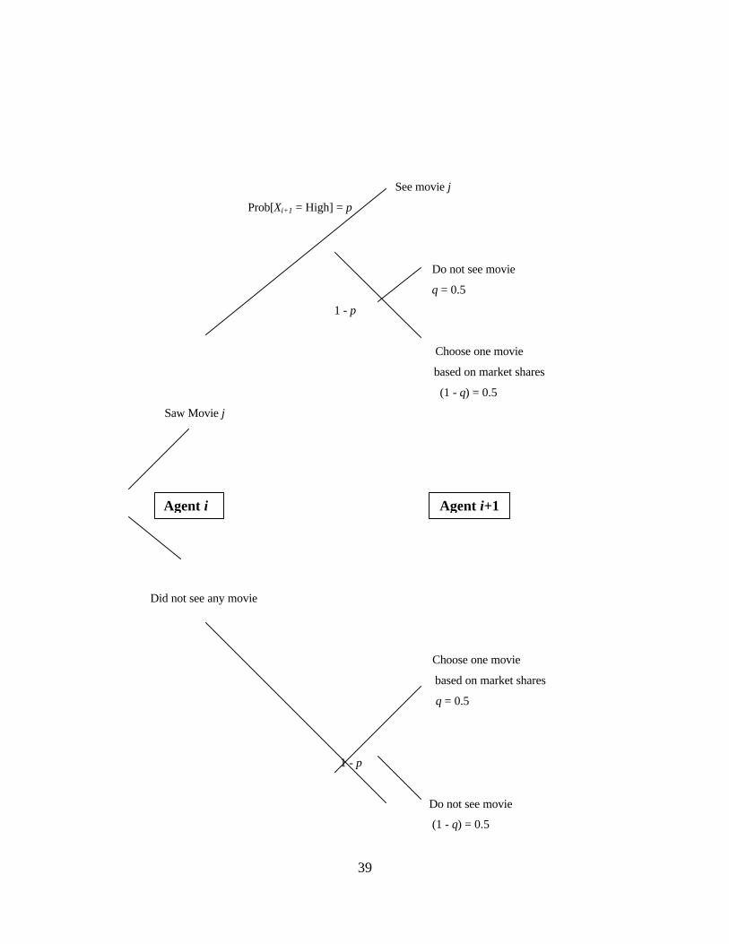
The formal structure of the model is as follows. Let there be a sequence of agents
i = 1, 2, 3, ... each deciding whether to see a movie j or not to see any movie at all [see
Figure 4]. There are m movies to choose from, i.e. j = 1, 2, 3,..., m. Agent i+1 observes
the action of agent i before her. If agent i chose movie j, agent i+1 will ask her about its
quality. If agent i tells agent i+1 that the movie is good, then there is a probability π that
agent i+1 will see the movie. We can interpret π as the confidence that agent i+1 attaches
to agent i's evaluation of movie j. A low π implies that agent i+1 might not have
confidence in agent i's evaluation. If this happens, there is a greater chance that agent i+1
will flip a fair coin to decide either to see one of the m movies or not to see a movie at all.

18
If agent i+1 decides on the former, she will choose a movie from a list movies with the
top n market shares (n < m and n takes values 5, 10 and 20).
Note that the number of movies with the top market shares changes over time. If,
at the initial stage, all movies have similar market shares, the number of movies with
market shares greater than or equal to the top n market shares may be large (greater than
n). However, if the distribution of agents becomes more uneven over time, the number of
movies with market shares greater than or equal to the top n market shares will shrink
toward n. The decision process for a bad movie is modeled similarly (see Figure 4). If
agent i did not see a movie, agent i+1 flips a fair coin to decide either to see a movie or
not to see any movie. If she decides on the former, she will choose randomly one movie
from the top n movies.
The exchange of quality information between agent i and agent i+1 is local.
However, when agent i+1 chooses to see a movie based on its market share she uses
aggregate information. If agent i+1 lacks her neighbor’s evaluation of a movie or has no
confidence in her neighbor’s evaluation, she resorts to the market shares of the leading n
movies to help her decide which movie to see.
In the model, the global information may encompass the market shares of all
movies (when n = m) or a subset of market shares of all movies (when n < m). The
important thing is that aggregate information evolves with the choices of agents. If
agents are evenly distributed across movies, aggregate information is diffuse and
uninformative. In contrast, if agents are unevenly distributed over movies, the top n
movies readily can be identified.
19
4.1. Accuracy of Signals and Informational Cascades
As in the simulations for the previous model, 2,000 agents are sequentially
allocated to 20 movies. Each movie is allocated one agent at the beginning. To begin the
simulation, the first of the 2,000 agents is allocated randomly to one of the 20 movies.
In situations where agents do not rely on a neighbor’s evaluation, they choose a movie
among those in the top-five (n = 5). We carry out twenty simulation runs for each value
of π from 0.5 to 0.9 with an increment of 0.05. Half the movies are good and half are
bad. The mean number of correct choices made by the agents for each value of π is given
in Table 3.
The mean proportion of correct choices declines as the confidence level π
declines; in fact, the proportion of correct choices is nearly identical to the accuracy of
the signal. The proportion of correct choices is higher when quality information is
available---the proportion of correct choices without quality information was only about
70% of signal accuracy, whereas it is about 100% of signal accuracy with quality
information. The transmission of information about quality increases the proportion of
correct choices that are made.
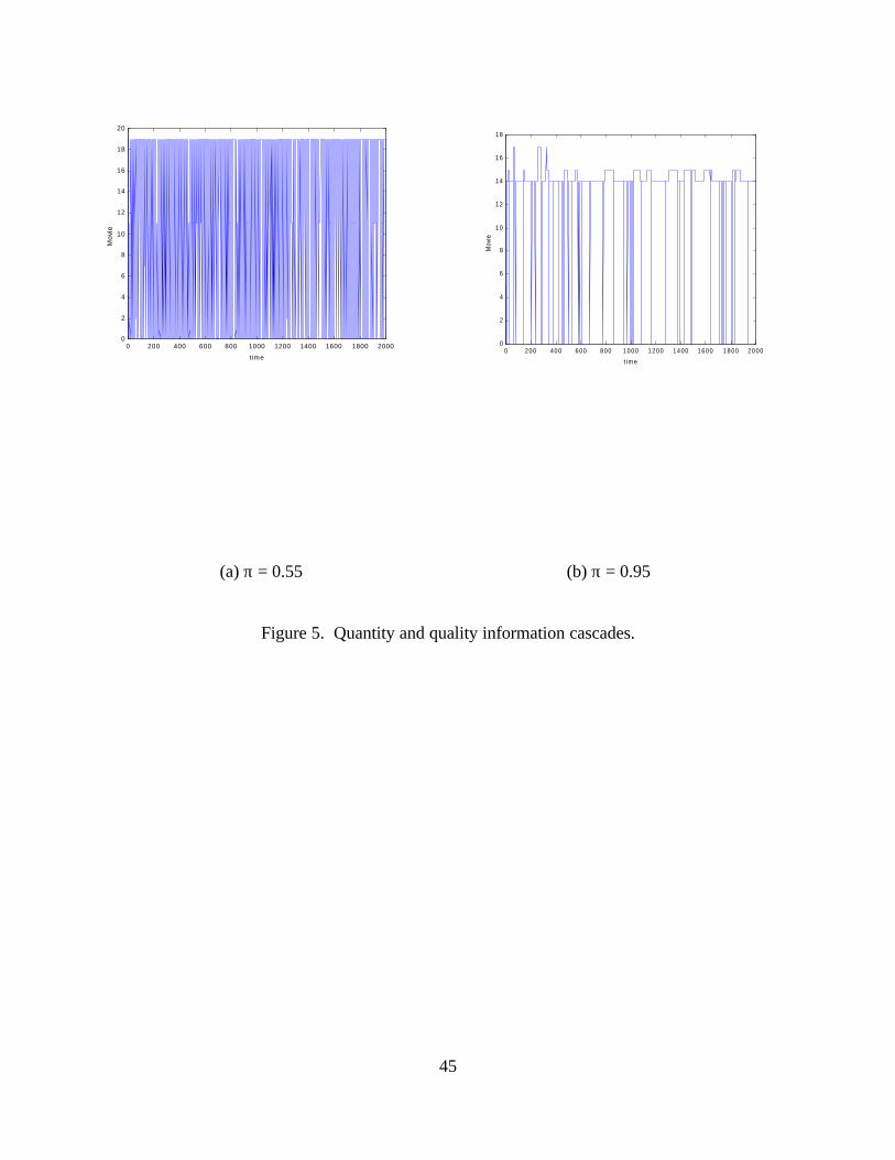
Do informational cascades occur more often in this model with quality and
quantity information than they do in the model with only quantity information? Figures 5
(a) and (b) are two examples from many simulations that illustrate a general conclusion.
Information cascades occur only when π is high. They are, however, very brief and more
than one movie has a cascade. This, in part, puts to rest the concern that, in the absence
of reliable quality information, movie audiences will look to box office numbers to
choose movies. Low accuracy in quality evaluation does not lead to herding on the box

20
office numbers. What low accuracy seems to do is to keep people from going to the
movies in the first place. The ability to choose “none of the above” is a powerful
constraint on audiences flocking to the box office leaders. If quality information is
accurate and a movie is good, then the dynamics can look like flocking because as
audience size grows, more quality information is transmitted and market share grows.
The growth in market share reinforces the process but it cannot drive it.
4.2. Information Cascades and Heavy Tails
Now we investigate the effect of the confidence level on the shape of the
distribution by varying the value of π and estimating α. Two thousand agents are
allocated to 200 movies. For each value of π, we run twenty simulations. The summary
statistics of our simulations are in Table 4.
The values of α generated by this quantity and quality signals model are lower
than those obtained with the quantity signal model. Because all the α values are less than
1, both the first and second moments of the box office distribution may not exist. An
interesting result is that the value of α first declines as π declines but later increases. The
reversal in the relationship between α and π occurs around π = 0.7. This suggests that
there may be a critical value of π at which the distribution of agents is maximally heavy-
tailed. Clearly, these cascades produce choice distributions that are too heavy-tailed to fit
the movies. In part, this is due to the assumption that half the movies are good and half
are bad. When most the movies are good or bad, the values of α are closer to the
empirical value of 1.5. We take this issue up below with fewer movies to look at the
dynamics more closely.

21
But, there is another factor that seems to be driving the cascade---the confidence
that agents place in quality information is exogenously set and independent of the weight
of the evidence contained in the aggregate information.
4.3. The Endogenous Transition between Local and Global Interactions
In the quality and quantity-based model agent i+1 switches from local to
aggregate information when she has little confidence in agent i's evaluation of a movie or
when she cannot get information from agent i about any of the movies available. In these
cases, she flips a coin to choose a movie with a large market share or no movie.
The switch from local to aggregate information is exogenously fixed by the
confidence level π. We extend that model to let the confidence that an agent attaches to
another’s assessment be endogenous. We assume that the larger the market share of
movie j, the greater confidence we place on agent i's evaluation of it (because it is
confirmed by many other choices). Then agent i+1 places confidence πij = movie j’s
market share in agent i’s quality assessment. The same confidence is placed in all agents.
Thus, if movie j's market share is very small, agent i+1 might not have confidence in
agent i's evaluation of it. We also assume that agents have bounded capabilities and can
keep track only of the top 5 movie shares (this is about what is reported on the evening
news).
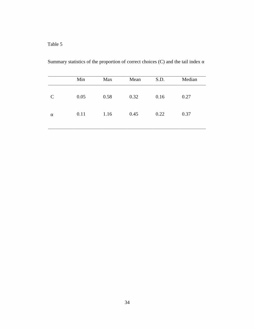
We do twenty simulations in which 2,000 agents are allocated to 200 movies and
obtain the mean value of the proportion of correct choices made using this model. Table
5 summarizes our results for both the mean value of the proportion of correct choices (C)
and the tail index (α).

22
The proportion of correct choices in this model with endogenous πij seems to be
low in comparison to the earlier models with π (confidence level) fixed or p (signal
accuracy) fixed. In the twenty simulation runs, none of the correct choices exceeded 58
percent. Similarly, the distribution is more heavy-tailed than in the previous models.
We plot C against α in Figure 6. The tail index α does not appear to be correlated
to the proportion of correct choices made. In other words, by making πij endogenous,
the system converges to a narrow range of values for α which are not related to the
proportion of correct choices made. This is a model of extreme cascades because, even
though quality information can be communicated, it carries weight only when market
share is high. The process spends too much time making random choices until market
shares begin to differentiate, if they do. If the shares do become differentiated enough for
a top 5 to emerge, a good movie in that group quickly captures a commanding lead
because the quality evaluations reinforce the market share signal. By adding a weight
that is non-linear in a movie’s market share to the confidence that an agent attaches to
another’s quality assessment, we obtain a dynamic that strongly selects good movies.
But, it drifts so long at low resolution that it makes a low percentage of correct choices.
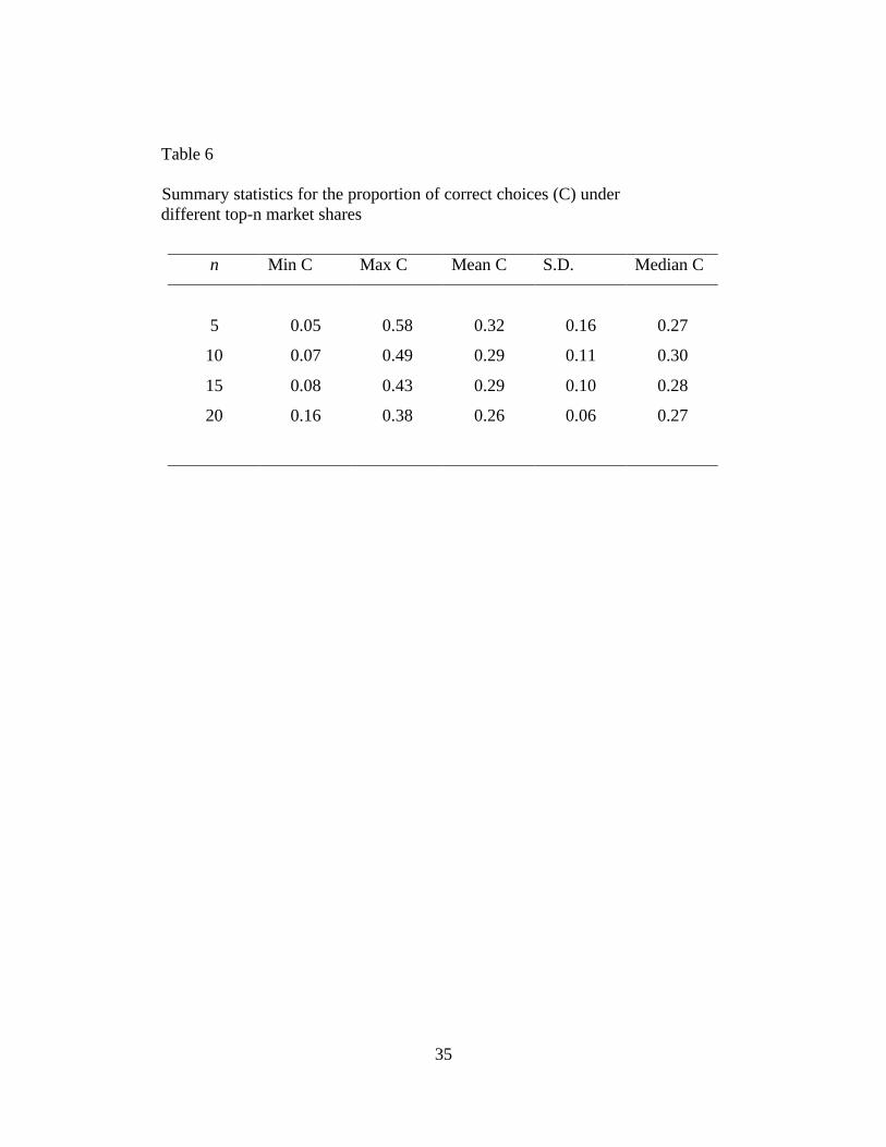
We run a series of simulations with different top-n market shares (n = 5, 10, 15,
and 20). Table 6 and 7 summarize our results. We observe that there is no discernible
relationship between n and C (Table 6). There is a slight increase in α (reflecting less tail
weight) as n increases.

23
5. A Closer Look at Dynamics and Initial Conditions
Several restrictive assumptions underlie the models we have studied so far. First,
we assumed that agents were uniformly distributed among movies to begin the
simulations. This is in sharp contrast with the actual situation in the movies, where the
distribution of theater screens and opening week revenue is highly uneven. Second, we
assumed that quality (good and bad) was evenly distributed among movies. These
assumptions may be too restrictive if we are interested in modeling the observed
dynamics and distributions of box office revenues in the motion picture industry. In this
section, we briefly explore the importance of these assumptions and how changing them
affect the results of the information cascade.
In analyzing these issues, we employ the quantity and quality model with
endogenous transition between local and global interactions. The global information is
the market shares of all movies. For simplicity, we simulate this model with 1,000
agents and 5 movies. With only 5 movies we cannot estimate the stability index, but we
can observe the dynamics in more detail. The simulations then are tournaments between
good and bad movies in which we vary the number of good versus bad. First, we assume
all movies are bad. Do we still get cascades?
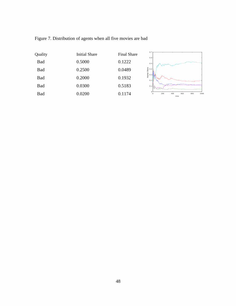
We seed the movies with opening market shares that are shown in the figures.
Figures 7 and 8 show two different dynamics from the same initial conditions. None of
the movies achieve a very high market share and there are evident crossing points where
one movie overtakes another. The dynamics do settle down and the final distribution of
audiences is quite uneven, and unrelated to the initial conditions. Of course, there is no

24
room for quality information to distinguish among movies since they are all bad. Most
people end up not going to a movie in this case.
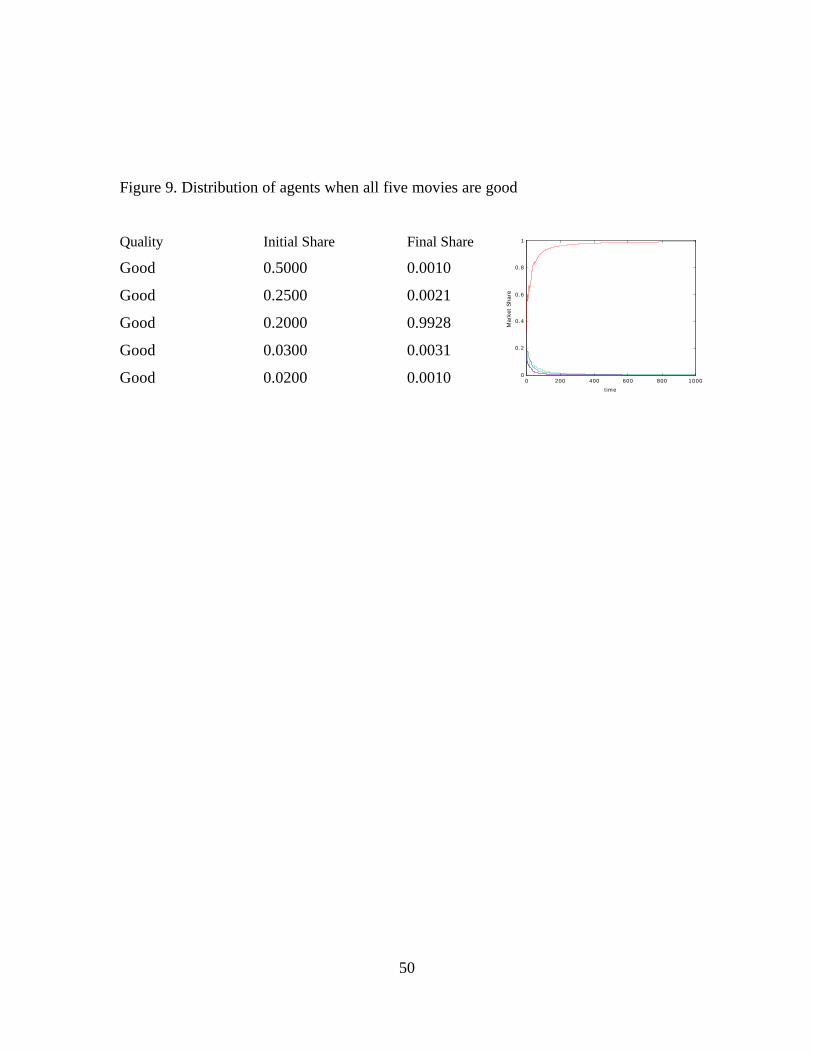
In contrast, if we assume that all movies are good then we begin to see cases
where a movie captures a substantial market share. Figures 9 and 10 summarize two
extreme examples where we assume that all movies are good. In Figure 9, the first movie
begins with an initial market share of 50 percent but ends with a final market share of
only 0.1 percent! However, a movie that began with a large initial market share can
increase its share further as shown in Figure 10. What these simulations show is that
extreme inequality in the distribution of agents can only occur when we have good
movies. In this case, word-of-mouth quality information does not distinguish among
movies, but market shares are reinforced by positive evaluations and become highly
credible signals of quality. Interestingly, now information cascades do occur and are
readily detected. This suggests that cascades are more likely when they are based on
correct information. This point is driven home in a series of additional simulations of bad
and good movies.
Figures 11, 12, 13 and 14 summarize what happens when we have a mixture of
good and bad movies. Figure 11 shows that a bad movie with large initial market share
may gain the highest market share, but generally will not. Its market share will never be
very large (typically well less than 50 percent and never higher than 60 percent).
Similarly, a good movie with small initial market share may (Figure 13) or may not
(Figure 14) gain the market. However, a good movie’s market share can be very
substantial (close to 99 percent as in Figure 13).

25
Figure 11 illustrates the “Godzilla” effect wherein a bad movie with a large
opening share of theater screens gains a substantial share, but one that is well below its
share at the opening. Figure 12 illustrates the “Full Monty” effect wherein a good movie
with a tiny opening gains a large following. Figure 13 illustrates the “Titanic” effect
wherein a good movie with a large opening share gains a large market share and kills the
other movies playing against it. Figure 14 tests your faith in people, just as the movies
always seem to do, for it depicts a good movie opening big and playing against only bad
movies that, nonetheless, goes on to mediocre results. Nearly every producer can name a
movie like this in her/his portfolio with high promise that died for inexplicable reasons.
Our answer is, “It’s the dynamics, stupid.” The individual characteristics of a movie are
not sufficient to determine how it will fare in the complex dynamics of the motion picture
market. Not a very satisfying answer for a movie executive to hear, but one that is closer
to the truth than any other answer that can be given.
How did a bad movie with only 2% of the opening go on to gain 58% of the
market against a good movie that opened with 50%? It happens; that’s the movies. In
this simulation there is an early period of extreme variation of market shares that weakens
the credibility of quality signals. That was enough to start an up cascade in the bad
movie and a down cascade in the good one. Once a bad movie gets a large share, the
share of good movies are too small a share for word-of-mouth evaluations to be credible.
So, even poor quality evaluations are not sufficient to overcome the power of the signal
contained in its market share. A bad movie can gain a large market share from purely
random circumstances. But, it is unlikely to become a monster hit like a good movie can.

26
How true to life are these sorts of complex dynamics? Very true, it turns out. To
give a sense of how variable this market is in Figure 15 we plot the data. The figure
shows the evolution of market shares for 115 films on Variety's top-50 list over a period
of 55 weeks (from 24 May 1996 to 12 June 1997). The figure looks like a mountain
range; there is a lot of low-level variation in the foothills topped with a few intermittent
peaks. In fact, like a mountain range, it is a fractal and the height variations are a power
law, often taken to be a signature self-organized behavior. Where are the cascades in
these figures? There are none; only one movie gets 40 % of the market and most movies
get far less than that. The extreme volatility one sees in these data is the antithesis of the
monotonous sequence of choices that would represent the work of an information
cascade.
Our model shows that a dynamical interaction among many, boundedly rational
agents exchanging quality and quantity information leads to extremely complex behavior
in the aggregate. In the real world of the movies, there is a further complication---new
movies are released each week throughout the year. The information cascades are
perturbed every week by new movies. Even the complicated and variable dynamics of
our simulated information cascades may not be complex enough to capture the
unpredictability that is the hallmark of the motion picture industry.
6. Conclusion
Information cascades are far more complex objects than standard models suggest
them to be. Their dynamics are richly varied and intermittent and they can go almost

27
anywhere. Cascades do not occur at the high frequency predicted by the models and they
do not converge as rapidly or as narrowly as the models suggest.
Cascades may coexist in a “intermittent equilibrium” in which they burst to the
lead and then give way to a rival and then return to the lead again. Because they are
intertwined and do not persist, cascades may be impossible to identify empirically. And,
it is impossible to predict the dynamic path or final outcome of a competition among
cascades because their basins of attraction are the stable distributions with an infinite
variance and, possibly, an infinite mean. It is because information cascade models are
able to generate stable distributions of outcomes that that they give a reasonable account
of the dynamics and frequency distribution of motion picture revenues. But, when the
dynamics of box office revenue leads to a stable Pareto-Lévy distribution with infinite
variance, anything can happen. Or, as screenwriter William Goldman famously said
about the movies, “No body knows anything.”
28
References
Anderson, L.R., Holt, C.A., 1997. Informational Cascades in the Laboratory. American
Economic Review 87, 847-862.
Bak, P., 1996. How Nature Works. Copernicus, New York.
Banerjee, A.V., 1992. A Simple Model of Herd Behavior. Quarterly Journal of
Economics 107, 797-817.
Bikhchandani, S., Hirshleifer, D., Welch, I., 1992. A Theory of Fads, Fashion, Custom,
and Cultural Change as Informational Cascades. Journal of Political Economy
100, 992-1026.
Chen, W-C., 1978. On Zipf’s Law. Ph.D. dissertation, University of Michigan.
Cont, R., Bouchaud, J-P, 1998. Herd Behavior and Aggregate Fluctuations in Financial
Markets. Unpublished.
De Vany, A., Walls, D., 1996. Bose-Einstein Dynamics and Adaptive Contracting in the
Motion Picture Industry. Economic Journal 106, 1493-1514.

29
De Vany, A., Walls, D., 1999a. Uncertainty in the Movies: Does Star Power Reduce the
Terror in the Box Office. Forthcoming, Journal of Cultural Economics.
De Vany, A., Walls, D., 1999b. Screen Wars, Star Wars, and Turbulent Information
Cascades at the Box Office. Unpublished.
Hill, B. M., 1974. The Rank-Frequency Form of Zipf’s Law. Journal of American
Statistical Association 69, 1017-1026.
Lee, C., 1999. Heavy-Tailed Distributions in the Motion Picture Industry. Unpublished
dissertation, Department of Economics, University of California, Irvine.
Lee, I. H., 1998. Market Crashes and Informational Avalanches. Review of Economic
Studies 65, 741-759.
Mandelbrot, B., 1997. Fractals and Scaling in Finance. Springer Verlag, New York.
Sornette, D., Zajdenweber, D., 1999. Economic Returns of Research: The Pareto law and
Its Implications. Unpublished.
Walls, D., 1997. Increasing Returns to information: Evidence from the Hong Kong movie
market. Applied Economic Letters 5, 215-219.
30
Table 1
Mean values of the proportion of correct choices (C) as
a function of signal accuracy (p)
Accuracy of Private Signal (p) C
0.95 0.64
0.90 0.49
0.85 0.45
0.80 0.61
0.75 0.47
0.70 0.44
0.65 0.49
0.60 0.50
0.55 0.53
0.50 0.49

31
Table 2
Summary statistics of tail index α from simulations
p Min α Max α Mean α S.D. α Median α
0.5 1.02 3.60 2.23 0.65 2.11
0.6 0.86 3.56 2.21 0.73 2.30
0.7 0.27 2.60 1.66 0.63 1.67
0.8 0.31 2.13 1.34 0.43 1.36
0.9 0.14 1.20 0.56 0.29 0.51

32
Table 3
The proportion of correct choices (C) under different confidence levels
Confidence Level (π) Mean C
0.95 0.95
0.90 0.86
0.85 0.85
0.80 0.82
0.75 0.77
0.70 0.74
0.65 0.66
0.60 0.64
0.55 0.63
0.50 0.58
Note: Global information involves top-5 market shares

33
Table 4
Summary statistics of tail index α from simulations
π Min α Max α Mean α S.D. α Median α
0.5 0.343 2.195 0.691 0.449 0.493
0.6 0.014 1.297 0.577 0.272 0.556
0.7 0.002 1.114 0.562 0.278 0.491
0.8 0.019 1.655 0.647 0.365 0.527
0.9 0.321 2.139 0.735 0.427 0.578
34
Table 5
Summary statistics of the proportion of correct choices (C) and the tail index α
Min Max Mean S.D. Median
C 0.05 0.58 0.32 0.16 0.27
α 0.11 1.16 0.45 0.22 0.37
35
Table 6
Summary statistics for the proportion of correct choices (C) under different top-n market shares
n Min C Max C Mean C S.D. Median C
5 0.05 0.58 0.32 0.16 0.27
10 0.07 0.49 0.29 0.11 0.30
15 0.08 0.43 0.29 0.10 0.28
20 0.16 0.38 0.26 0.06 0.27

36
Table 7
Summary statistics for the tail index α under different top-n market shares
n Min α Max α Mean α S.D. Median α
5 0.11 1.16 0.45 0.22 0.37
10 0.04 0.89 0.40 0.18 0.37
15 0.06 0.90 0.48 0.18 0.49
20 0.14 1.47 0.78 0.36 0.86

37
00.2
0.40.6
0.81
Prior1
2
3
4
5
N
0
0.2
0.4Cascade
00.2
0.40.6
0.81
Prior
Figure 1. The ex ante probability that a cascade will not occur as a
function of the signal accuracy and the number of agents

38
39
See movie j
Prob[Xi+1 = High] = p
Do not see movie
q = 0.5
1 - p
Choose one movie
based on market shares
(1 - q) = 0.5
Saw Movie j
Did not see any movie
Choose one movie
based on market shares
q = 0.5
1 - p
Do not see movie
(1 - q) = 0.5
Agent i+1Agent i

40
Prob[Xi+1 = Low] = p
Do not see movie
Figure 2. A simple BHW model

41
when p = 0.55 (b) when p = 0.95
(a) (b)
(a) Low accuracy (b) High accuracy
Figure 3. Informational cascades among 20 movies
0 200 400 600 800 1000 1200 1400 1600 1800 20000
2
4
6
8
10
12
14
16
18
time
Mov
ie
0 200 400 600 800 1000 1200 1400 1600 1800 20002
4
6
8
10
12
14
16
18
20
time
Mov
ie

42

43
See movie j
π
Do not see movie
1 - π q = 0.5
quality = Good
Choose one movie
from list of top-n
market shares
(1 - q) = 0.5
Seen Movie j
Choose one movie
from list of top-n
quality = Bad market shares
1 - π q = 0.5
Do not see movie
(1 - q) = 0.5
π
Do not see movie
Choose one movie from
Agent i
Agent i+1
Agent i+1

44
list of top-n market shares
q = 0.5
Did not see
a movie
Do not see a movie
(1 - q) = 0.5
Figure 4. The quantity- and quality-based model
Agent i+1
45
(a) π = 0.55 (b) π = 0.95
Figure 5. Quantity and quality information cascades.
0 200 400 600 800 1000 1200 1400 1600 1800 20000
2
4
6
8
10
12
14
16
18
time
Mov
ie
0 200 400 600 800 1000 1200 1400 1600 1800 20000
2
4
6
8
10
12
14
16
18
20
time
Mov
ie

46
Figure 6. Proportion of correct choices (C) vs. tail index (α).
alph
a
C.0495 .5825
.1122
1.1572

47
48
Figure 7. Distribution of agents when all five movies are bad
Quality Initial Share Final Share
Bad 0.5000 0.1222
Bad 0.2500 0.0489
Bad 0.2000 0.1932
Bad 0.0300 0.5183
Bad 0.0200 0.1174 0 200 400 600 800 10000
0.1
0.2
0.3
0.4
0.5
0.6
0.7
time
Mar
ket
Sha
re

49
Figure 8. Distribution of agents when all five movies are bad
Quality Initial Share Final Share
Bad 0.5000 0.4929
Bad 0.2500 0.0738
Bad 0.2000 0.1381
Bad 0.0300 0.0548
Bad 0.0200 0.2405 0 200 400 600 800 10000
0.1
0.2
0.3
0.4
0.5
time
Mar
ket
Sha
re
50
Figure 9. Distribution of agents when all five movies are good
Quality Initial Share Final Share
Good 0.5000 0.0010
Good 0.2500 0.0021
Good 0.2000 0.9928
Good 0.0300 0.0031
Good 0.0200 0.0010 0 200 400 600 800 10000
0.2
0.4
0.6
0.8
1
time
Mar
ket
Sha
re

51
Figure 10. Distribution of agents when all five movies are good
Quality Initial Share Final Share
Good 0.5000 0.9904
Good 0.2500 0.0043
Good 0.2000 0.0011
Good 0.0300 0.0021
Good 0.0200 0.0021 0 200 400 600 800 10000
0.2
0.4
0.6
0.8
1
time
Mar
ket
Sha
re

52
Figure 11. Distribution of agents when one movie is bad, the rest are good
Quality Initial Market Share Final Market Share
Bad 0.5000 0.4303
Good 0.2500 0.0283
Good 0.2000 0.0586
Good 0.0300 0.3172
Good 0.0200 0.1657 0 200 400 600 800 10000
0.1
0.2
0.3
0.4
0.5
0.6
0.7
time
Mark
et S
hare

53
Figure 12. Distribution of agents when one movie is bad, the rest are good
Quality Initial Market Share Final Market Share
Bad 0.5000 0.0391
Good 0.2500 0.0046
Good 0.2000 0.0080
Good 0.0300 0.0057
Good 0.0200 0.9425 0 200 400 600 800 10000
0.2
0.4
0.6
0.8
1
time
Mar
ket
Sha
re

54
Figure 13. Distribution of agents when one movie is good, the rest are bad
Quality Initial Market Share Final Market Share
Good 0.5000 0.9883
Bad 0.2500 0.0032
Bad 0.2000 0.0021
Bad 0.0300 0.0021
Bad 0.0200 0.0042 0 200 400 600 800 10000
0.2
0.4
0.6
0.8
1
time
Mar
ket
Sha
re

55
Figure 14. Distribution of agents when one movie is good, the rest are bad
Quality Initial Market Share Final Market Share
Good 0.5000 0.1358
Bad 0.2500 0.0515
Bad 0.2000 0.0656
Bad 0.0300 0.1639
Bad 0.0200 0.58310 200 400 600 800 1000
0
0.1
0.2
0.3
0.4
0.5
0.6
0.7
time
Mar
ket
Sha
re

56

57
Figure 15. Market Shares of 115 films on the Variety's top-50 list
over 55 weeks (24 May 1996 to 12 June 1997)
0
0.05
0.1
0.15
0.2
0.25
0.3
0.35
0.4
0.45
1 3 5 7 9 11 13 15 17 19 21 23 25 27 29 31 33 35 37 39 41 43 45 47 49 51 53 55
Week
Mar
ket
Sh
are


