
Journal of Engineering Volume 21 September 2015 Number 9
34
Impact of Aggregate Gradation and Filler Type on Marshall Properties of
Asphalt Concrete
Saad Issa Sarsam Kadhum Hulial Sultan Professor MSc. student College of engineering- University of Baghdad College of engineering- University of Baghdad E-mail: [email protected] E-mail: [email protected]
ABSTRACT
As asphalt concrete wearing course (ACWC) is the top layer in the pavement structure, the
material should be able to sustain stresses caused by direct traffic loading. The objective of this
study is to evaluate the influence of aggregate gradation and mineral filler type on Marshall
Properties. A detailed laboratory study is carried out by preparing asphalt mixtures specimens
using locally available materials including asphalt binder (40-50) penetration grade, two types of
aggregate gradation representing SCRB and ROAD NOTE 31 specifications and two types of
mineral filler including limestone dust and coal fly ash. Four types of mixtures were prepared
and tested. The first type included SCRB specification and limestone dust, the second type
included SCRB specification and coal fly ash, the third types included ROAD NOTE 31
specification and limestone dust and the fourth type included ROAD NOTE 31 specification and
coal fly ash. The optimum asphalt content of each type of mixtures was determined using
Marshall Method of mix design. 60 specimen were prepared and tested with dimension of 10.16
cm in diameter and 6.35 cm in height. Results of this study indicated that aggregate gradation
and filler type have a significant effect on optimum asphalt content and Marshall Properties.
From the experimental data, it was observed that the value of Marshall Stability is comparatively
higher when using fly ash as filler as compared to limestone dust.
Keywords: asphalt concrete mixture, aggregate gradation, mineral filler, Marshall Properties.
اختلاف تذرج انركبو ونوع انبدة انبنئة عهى خصبئص يبرشبل نهخرسبنة الاسفهتيةتأثير
طبسعذ عيسى سرسى كبظى ههيم سه
شاسخبر طبنب يبخسخ
لسى انهذست انذت –كهت انهذست -لسى انهذست انذت خبيعت بغذاد –كهت انهذست -خبيعت بغذاد
خلاصةان
ا حكى انىاد انسخخذيت لبدسة عهى يمبويت وهزا خطهب ه انطبمت انعهب ف حشكم انشصفت تالاسفهخانخشسبت ا طبمت
الاخهبداث انبحدت ع حشكت انشوس انعبنت انببششة. انهذف انشئس ي انبحث هى ححذذ حبثش اخخلاف انخذسج وىع انبدة
ت الاسفهخت انبنئت عهى خصبئص يبسشبل نهخشسبت الاسفهخت. انذساست انخخبشت انفصهت فزث بخحضش برج ي انخشسب
( وىع ي حذسج انشكبو انز 04-04اسفهج سج رو الاخخشاق )ع طشك اسخخذاو يىاد يخىفشة يحهب وانخ حخظ
ثلا انىاصفت انعشالت نهطشق واندسىس وانىاصفت انبشطبت وكزنك حى اسخخذاو ىع ي انبدة انبنئت وانز ثلا
حى ححضش اسبعت اىاع ي انخهطبث, كبج انخهطت الاونى يكىت ي حذسج د انفحى انخطبش.غببس انحدش اندشي وسيب
يىاصفت انطشق واندسىس وغببس انحدش اندشي وانثبت يكىت ي حذسج يىاصفت انطشق واندسىس وسيبد انفحى انخطبش

Journal of Engineering Volume 21 September 2015 Number 9
35
بعت يكىت ي حذسج انىاصفت انبشطبت وسيبد وانثبنثت يكىت ي حذسج انىاصفت انبشطبت وغببس انحدش اندشي وانشا
04حى ادبد سبت الاسفهج انثهى نكم ىع ي انخهطبث ببسخخذاو طشمت حصى يبسشبل. حى ححضش وفحص انفحى انخطبش.
هب حبثش كبش سى . اظهشث خبئح هز انذساست انى ا حذسج انشكبو وىع انبدة انبنئت ن 0,,0سى واسحفبع 04,00ىرج بمطش
عهى خصبئص يبسشبل وسبت الاسفهج انثبنت. نىحع اضب ا لت ثببث يبسشبل اعهى سبب عذ اسخخذاو سيبد انفحى
انخطبش كبدة يبنئت بذلا ع غببس انحدش اندشي.
خصبئص يبسشبل.خهطت انخشسبت الاسفهخت, حذسج انشكبو, انبدة انعذت انبنئت, : ت انرئيسيهانكهب
1. INTRODUCTION In order to provide comfortable ride and withstand the effects arising from traffic loading
and climate, pavement materials should be designed to achieve a certain level of performance
and the performance should be maintained during the service life, Zhi Suo and Wing, 2008.
Fillers as one of the components in an asphalt mixture, play a major role in determining the
properties and the behavior of the mixture, especially the binding and aggregate interlocking
effects, Sarsam, 1984. Mineral fillers serve a dual purpose when added to asphalt mixes, the
portion of the mineral filler that is finer than the thickness of the asphalt film blends with asphalt
cement binder to form a mortar or mastic that contributes to improved stiffening of the mix.
Particles larger than the thickness of the asphalt film behave as mineral aggregate and hence
contribute to the contact points between individual aggregate particles, Puzinauskas, 1969. In
general, filler have various purposes among which, they fill voids and hence reduce optimum
asphalt content and increase stability, meet specifications for aggregate gradation, and improve
bond between asphalt cement and aggregate, Bouchard, 1992. Gradation is defined as the
distribution of particle sizes expressed as a percent of the total weight. If the specific gravities of
the aggregates used are similar, the gradation in volume will be similar to the gradation in
weight.
2. RESEARCH OBJECTIVE
The objective of this research is to investigating the influence of using two types of
aggregate gradation and two types of mineral filler on optimum asphalt content and Marshall
Properties.
3. BACKGROND
Ali et al. 1996 investigated the effects of fly ash on the material and mechanical properties
of asphalt mixtures; results from this study indicated that fly ash can be used as a mineral filler to
improve resilient modulus characteristics and stripping resistance. Sarsam, 2015, studied the
effect of adding nano material such as fly ash and silica fumes on the properties of asphalt
cement, it was concluded that such nano materials have positive effect on asphalt cement
rheological properties. Sarsam, 2013 concluded that nano materials such as coal fly ash and lime
have improved the physical properties of asphalt cement. Kallas and Puzinauskas, 1967
believed that filler performed a dual role in asphalt-aggregate mixtures. A portion of the filler
with particles larger than the asphalt film will contribute in producing the contact points between
aggregate particles, while the remaining filler is in colloidal suspension in the asphalt binder,
resulting in a binder with a stiffer consistency. They also found that the stabilities of asphalt
mixtures increased up to a certain filler concentration, then decrease with additional filler. A

Journal of Engineering Volume 21 September 2015 Number 9
36
study was made by Matthews and Monismith, 1992 on effects of gradation on the asphalt
content where both wearing and binder mixes were considered. Further, they have carried out
regression analysis on test data to investigate the relationship between asphalt content and
gradation. Their study shows that no correlation exists between asphalt content and the percent
passing the 4.75mm (No. 4) and 2.36mm (No. 8) sieves for the wearing mix. On the other hand,
for binder mixes there exists a relationship between changes in gradation and measured asphalt
content that shows as the mix becomes finer for the given sieve size, the asphalt content
increases. Roberts et al., 1996 suggested that gradation is perhaps the most important property
which affects almost all the important properties of a bituminous mixture, including stiffness,
stability, durability, permeability, workability, fatigue resistance, frictional resistance, and
resistance to moisture damage. Sarsam, 1987 studied the effect of various gradations on
Marshall properties of asphalt concrete, it was concluded that gap gradation exhibit more
stability and low flow values when compared to dense graded mixes.
4. MATERIAL CHARACERISTIC
4.1 Asphalt Cement
Asphalt cement of (40-50) penetration grade from Nasiriya refinery was used in this work.
The physical properties of original asphalt cement are presented in Table 1.
4.2 Aggregate
Coarse and fine aggregates were obtained from AL-Ukhaydir- Karbala quarry; their
physical properties are listed in Table 2.
4.3 Mineral Filler
Two types of mineral filler were used in this work; limestone dust produced in the lime
factory in Karbala governorate and coal fly ash obtained from local market. Table 3 shows
major physical properties.
4.4 Selection of Design Aggregate Gradation
The selected gradation in this work followed the SCRB, 2003 specification, with 12.5 (mm)
nominal maximum size and ROAD NOTE 31, 1993 specification with 12.5 (mm) nominal
maximum size. Fig.1, Fig. 2, Table 4 and Table 5 show selected aggregate gradation. The
implementation of both aggregate gradations in this research work could aid in understanding the
effect of environmental condition on physical properties of asphalt concrete since the SCRB
specification is recommended for hot climate, while ROAD NOTE 31 is recommended for cold
climate condition.
4.5 Preparation of Marshall Specimen
Four groups of Marshall Specimens were prepared and used in this work to obtain optimum
asphalt binder content; five percentages of asphalt cement (3.5, 4, 4.5, 5 and 5.5) % and 15
specimen were used for each type of mixture. These four groups of mixture were tested for
determination of optimum asphalt requirements as follows:
Journal of Engineering Volume 21 September 2015 Number 9
37
a.) Determine the optimum asphalt binder content for SCRB grading specification and using
limestone dust as a mineral filler, Mixture Type I.
b.) Determine the optimum asphalt binder content for SCRB grading specification and using coal
fly ash as a mineral filler, Mixture Type II.
c.) Determine the optimum asphalt binder content for ROAD NOTE 31 grading specification and
using limestone dust as a mineral filler, Mixture Type III.
d.) Determine the optimum asphalt binder content for ROAD NOTE 31 grading specification
and using coal fly ash as a mineral filler, Mixture Type IV.
60 specimens were used in this work to determine optimum asphalt binder content, The
specimens were prepared in accordance with (ASTM D1559), Marshall mold, spatula, and
compaction hammer were heated on a hot plate to a temperature between (140-150 ºC). The
aggregate was first sieved, washed, and dried to a constant weight at 110 ºC. Coarse and fine
aggregates were combined with mineral filler to meet the specified gradation in section (4.4).
Aggregates and filler were heated to (160 ºC), asphalt was heated up to (150) ºC prior to mixing,
and it was added to the hot aggregate and mixed for two minutes on hot plate until all aggregate
particles were coated with asphalt cement. The compaction temperature was (140) ºC, which
gives a viscosity (280 30) cSt. The (75) blows of compaction hammer are applied with a free
fall of 4.536 kg (10 lb) sliding weight and a free fall of (457.2) mm. After compaction, the base
plate is removed and the same blows are applied to the bottom of the specimen that has been
turned around. The specimen in mold was left to cool at room temperature for 24 hours, then it
was extracted from the mold using mechanical jack. Fig. 3 shows preparation of Marshall
Specimens.
4.6 Testing of Marshall Specimens
4.6.1 Determination of maximum theoretical specific gravity
The purpose of conducting this test is to determine the maximum theoretical specific gravity
of loose HMA specimens. The maximum theoretical specific gravity was determined according
to (ASTM D2041-03). 1500 gm was needed in this test for each type of mixture with maximum
nominal aggregate size of (12.5 mm). This test was conduct for each percent of asphalt content (
3.5, 4, 4.5, 5 and 5.5 )%. Fig. 4 presents the apparatus used to obtain maximum specific gravity.
4.6.2 Determination of flow and stability of specimens
Procedure of preparing and testing specimens was according to (ASTM D1559) .This
method covers the measure of the resistance to plastic flow of cylindrical specimens (2.5 in.
height × 4.0 in. diameter) of asphalt paving mix after conditioning in water bath at 60 °C for 30
minute. A load was applied with a constant rate of (50.8) mm/min until the maximum load was
reached. The maximum load resistance and the corresponding strain values were recorded as
Marshall stability and flow respectively. Three specimens for each type of mixture were
prepared and tested and average results are reported. Fig. 5 shows Marshall apparatus of this test.

Journal of Engineering Volume 21 September 2015 Number 9
38
5. DISCUSSION OF TEST RESULTS
5.1 Optimum Asphalt Content (OAC)
The optimum asphalt content was 4.9 %, 4.7 %, 4.7 % and 4.5 % for mixtures type I, type II,
type III and type IV respectively. The Marshall Properties which are considered to select the
optimum asphalt content; stability, bulk density, and air voids, while other properties; flow,
VMA, and VFA are considered to confirm the required limits by SCRB specification.
5.2 Marshall Stability
Stability is an important property of the asphalt mixture in the wearing course design.
Marshall Stability gives the indication about the resistance of asphalt mixture to permanent
deformation, a high value of Marshall stability indicates increased Marshall Stiffness. The high
stiffness of asphalt mixture means good resistance to traffic loadings but it also indicates lower
flexibility which is required for long term performance, high stiffness values are not
recommended due to thermal cracking which expected to occur in future. Fig. 6 shows the effect
of aggregate gradation and filler type on Marshall stability. It is noted that the Marshall stability
was increased by 13.39% when using fly ash as a mineral filler instead of limestone dust with
SCRB gradation and it was increased by 32.63 % when using fly ash as a mineral filler when
compared to mix with limestone dust with ROAD NOTE 31 gradation. such results comply with
the findings of Pradan and Roy, 2008. Also, It is noted that the Marshall stability was
decreased by 15.17 % when using ROAD NOTE 31 gradation as compared with SCRB
gradation with using limestone dust as a mineral filler, while it was decreased by 0.78 % when
using ROAD NOTE 31 gradation instead of SCRB gradation with using coal fly ash as a
mineral filler. The data are listed from Table 6 to Table 9.
5.3 Marshall Flow
Generally, high flow values indicate a plastic mix that is more prone to permanent
deformation problem due to traffic loads, whereas low flow values may indicate a mix with
higher than normal voids and insufficient asphalt for durability and could result premature
cracking due to mixture brittleness during the life of the pavement. Fig.7 shows the effect of
aggregate gradation and filler type on Marshall flow. It can be observed that the Marshall flow
was increased by 24.13 % when using fly ash as a mineral filler instead of limestone dust with
SCRB, 2003 gradation. such results comply with the findings of Rahman and Sobhan, 2013.
and Kar et al., 2014. Also it is also noted that the Marshall flow was decreases by 6.06 % when
using fly ash as a mineral filler instead of limestone dust with ROAD NOTE 31 gradation. such
results comply with the findings of Pradan and Roy, 2008. Also, it is noted that the Marshall
flow was decreases by 13.79 % when using SCRB gradation Instead of ROAD NOTE 31
gradation with using limestone dust as a mineral filler, while Marshall flow was increases by
13.88 % when using SCRB grading Instead of ROAD NOTE 31 gradation when using fly ash as
a mineral filler. The data are listed from Table 6 to Table 9.

Journal of Engineering Volume 21 September 2015 Number 9
39
5.4 Bulk Density
In the Marshall Mix design procedure, the density varies with asphalt content in such a way
that it increases with increasing asphalt content in the mixture. The density reaches a peak and
then begins to decrease because additional asphalt cement produces thicker films around the
individual aggregates, and tend to push the aggregate particles further apart subsequently
resulting lower density. The effect of aggregate gradation and filler type on bulk density is
illustrated in Fig.8. This figure indicates that the bulk density increases when using fly ash as a
mineral filler for both SCRB gradation and ROAD NOTE 31 gradation. It is also found that the
bulk density was decreased when using SCRB gradation as compared to ROAD NOTE 31
gradation when using limestone dust as a mineral filler, and it is noted that the bulk density was
decreased when using SCRB grading as compared to ROAD NOTE 31 gradation when using fly
ash as a mineral filler. The data are listed from Table 6 to Table 9.
5.5 Voids in Total Mixture ( VTM %)
Air void in the mixture is an important parameter because it permits the properties and
performance of the mixture to be predicted for the service life of the pavement, and percentage
of air voids is related to durability of asphalt mixture. Air void proportion around 4% is enough
to prevent bleeding or flushing that would reduce the skid resistance of the pavement and
increase fatigue resistance susceptibility. Fig. 9 shows the effect of aggregate gradation and filler
type on voids in total mix (VTM) percent’s. It is clear from the figure that the air void was
decreased when using fly ash as a mineral filler as compared to limestone dust with SCRB
gradation. such results comply with the findings of Kar et al., 2014, while when using fly ash as
a mineral filler with ROAD NOTE 31 gradation, air void is increases. such results comply with
the findings of Rahman and Sobhan, 2013. It is also found that the air void is decreases when
using ROAD NOTE 31 gradation with using limestone dust as a mineral filler, and it is noted
that the air void is increases when using ROAD NOTE 31 gradation with fly ash as a mineral
filler. The data are listed from Table 6 to Table 9.
5.6 Voids Filled with Asphalt (VFA%)
Voids filled with asphalt (VFA) are the void spaces that exist between the aggregate particles
in the compacted paving asphalt mixture that are filled with binder. The purpose for the VFA is
to avoid less durable asphalt mixtures resulting from thin films of binder on the aggregate
particles in light traffic situations. Fig. 10 shows the effect of aggregate gradation and filler type
on void filled with asphalt. It indicates that void filled with asphalt was increased when using fly
ash as a mineral filler with SCRB gradation. Such results comply with the findings of Rahman
and Sobhan, 2013, while when using fly ash as a mineral filler with ROAD NOTE 31 gradation,
void filled with asphalt was decreased. It is also noted that void filled with asphalt was decreased
when using ROAD NOTE 31gradation with using both limestone dust and coal fly ash as a
mineral filler. The data are listed from Table 6 to Table 9.

Journal of Engineering Volume 21 September 2015 Number 9
40
5.7 Voids in Mineral Aggregate ( VMA%)
The voids in the mineral aggregate is the total available volume of voids between the
aggregate particles in the compacted paving mixture that includes the air voids and the voids
filled with effective asphalt content expressed as a percent of the total volume. It is significantly
important for the performance characteristics of a mixture for any given mixture, the VMA must
be sufficiently high enough to ensure that there is space for the required asphalt cement, for its
durability purpose, and air space. If the VMA is too small, there will be no space for the asphalt
cement required to coat around the aggregates and this subsequently results in durability
problems. On the other hand, if VMA is too large, the mixture may suffer stability problems.
Fig.11 shows the effect of aggregate gradation and filler type on void in mineral aggregate
(VMA). It is clear from the figure that voids in mineral aggregate were decreased when using
fly ash as mineral filler with both SCRB and ROAD NOTE 31 gradation. It is noted that the void
in mineral aggregate was decreased when using ROAD NOTE 31 gradation instead of SCRB
gradation when using both limestone dust and coal fly ash as a mineral filler. Such results
comply with the findings of Kar et al., 2014. The data are listed from Table 6 to Table 9.
6. CONCLUSION
1. Optimum asphalt content requirement was lower when coal fly ash was implemented as a
mineral filler at both types of aggregate gradation SCRB and ROAD NOTE 31
specifications.
2. Optimum asphalt content requirement for grading of ROAD NOTE 31 specification was
lower than SCRB specification at both types of mineral filler limestone dust and coal fly
ash.
3. Marshall stability was increased by 13.39% and 32.63% when using fly ash as a mineral
filler instead of limestone dust with both types of aggregate gradation (SCRB and ROAD
NOTE 31) gradation. On the other hand, Marshall stability was decreased by 15.17 %
and 0.78% when using ROAD NOTE 31 gradation as compared with SCRB gradation for
both types of mineral filler limestone dust coal fly ash.
4. Marshall flow was increased by 24.13 % when using fly ash as a mineral filler instead of
limestone dust with SCRB gradation, while it was decreased by 6.06 % when using fly
ash as a mineral filler instead of limestone dust with ROAD NOTE 31 gradation.
5. Marshall flow was decreased by 13.79 % when using SCRB gradation instead of ROAD
NOTE 31 gradation with using limestone dust as a mineral filler, while it was increased
by 13.88 % when using SCRB grading instead of ROAD NOTE 31 gradation when using
fly ash as a mineral filler.
6. Bulk density increases when using fly ash as a mineral filler for both SCRB gradation
and ROAD NOTE 31 gradation.
7. Bulk density was decreased when using SCRB gradation as compared to ROAD NOTE
31 gradation for both limestone dust and coal fly ash.

Journal of Engineering Volume 21 September 2015 Number 9
41
REFFRENCES
Ali N, Chan JS, Simms S, Bushman R, Bergan AT, 1996, Mechanistic evaluation of fly
ash asphalt concrete mixtures. Journal of Materials in Civil Engineering, ASCE 8(1):19-
25.
Bouchard, G. P., 1992, Effect of Aggregates and Mineral Fillers On asphalt Mixtures
Performance, ASTM, STP 1147, Richard C. Meininger, Ed., American Society for
Testing and Material, Philadelphia.
BS. 1993 A guide to the structural design of bitumen surfaced roads in tropical and sup
tropical countries, ROAD NOTE 31, Transport research laboratory, Crowthorne,
Berkisher, United kingdom.
Kar D., Panda M. and Giri J. P., 2014, Influence of Fly Ash as a Filler in Bituminous
Mixes, Department of Civil Engineering, NIT Rourkela, Odisha, India.
Kallas BF, Puzinauskas VP, 1967, A study of mineral fillers in asphalt paving mixtures.
Proceedings of the Association of Asphalt Paving Technologists 36:493-528.
Matthews, J. M. and Monismith, C. L., 1992, The Effect of Aggregate Gradation on the
Creep response of Asphalt Mixtures and Pavement Rutting Estimates, Effect of
Aggregates and Mineral Fillers On asphalt Mixtures Performance, ASTM STP 1147,
Richard C. Meininger, Ed., American Society for Testing and Material, Philadelphia.
Pradan and Roy, 2008, Effect of Fillers on bituminous paving Mixes, Bachelor of
Technology in Civil Engineering, National Institute of Technology.
Puzinauskas, V.P., 1969. Filler in Asphalt Mixtures. The Asphalt Institute Research
Report 69-2, Lexington, Kentucky.
Rahman M.N. and M.A. Sobhan, 2013, Use of Non-Conventional Fillers on Asphalt-
Concrete Mixture, Department of Civil Engineering, Rajshahi University of Engineering
and Technology, Rajshahi-6204, Bangladesh.
Roberts, F. L., Kandhal, P. S., Brown, E. R., Lee, D., and Kennedy, T., 1996, Hot Mix
Asphalt Materials, Mixtures Design, and Construction, NAPA Education Foundation,
Lanham, Maryland. First Edition, pp. 241-250.
Sarsam S. 1987, Effect of various gradations on the properties of Asphaltic Concrete
using two design methods, Indian Highways IRC Vol. 15 No.10.India.
Sarsam S. 1984, A study of mineral filler in dense graded Asphalt Concrete, Indian
Highways IRC Vol. 12 No.12. India.

Journal of Engineering Volume 21 September 2015 Number 9
42
Sarsam S., 2013, Improving Asphalt Cement Properties by Digestion with Nano
materials, Research and Application of Material Journal, RAM, Vol.1, No.6, (P 61-64).
Sciknow Publications Ltd. USA.
Sarsam S. 2015, Impact of Nano Materials on Rheological and Physical Properties of
Asphalt Cement, International Journal of Advanced Materials Research, Public science
framework, American institute of science, Vol. 1, No. 1, pp. 8-14, USA.
State Commission of Roads and Bridges SCRB, 2003. Standard Specification for Roads
& Bridges, Ministry of Housing & Construction, Iraq.
Zhi Suo, Wing Gun Wong, 2008, Analysis of fatigue crack growth behavior in asphalt
concrete material in wearing course, Construction and Building Materials, Available
online 20 February.
Table 1. Physical properties of asphalt cement.
Table 2. Physical properties of aggregate.
Property
Coarse aggregate Fine aggregate
Test Result
ASTM
Designation
No.
Test
Result
ASTM
Designation
No.
Bulk Specific Gravity 2. 542 ASTM C
127
2.558
ASTM C 128 Apparent Specific Gravity 2.554 2.563
Water Absorption % 1.076 % 1.83 %
Wear % (Los Angeles
Abrasion) 17.92 %
ASTM C
131 ---- ----
Property Unit Test Result SCRB (2003)
Specifications
Penetration, (25˚C, 100 gm, 5 sec) ASTM D
5 0.1 mm 42 40 – 50
Softening point (Ring & Ball) ASTM D 36 49 ----
Ductility (25 ˚ C, 5 cm/min) ASTM D 113 cm 140 >100
Specific gravity 25˚C ASTM D70 ---- 1.04 ----
Flash point (cleave land open cup) ASTM
D 92 256 >232
After Thin - Film Oven Test ASTM D 1754
Retained Penetration of Residue (25 ˚C ,
100 gm , 5 sec) % 67 >55%
Ductility (25 ˚ C , 5 cm/min) cm 83 >25
Loss on Weight % (163 ˚ C , 50 gm , 5 hr) % 0.35 ----
Journal of Engineering Volume 21 September 2015 Number 9
43
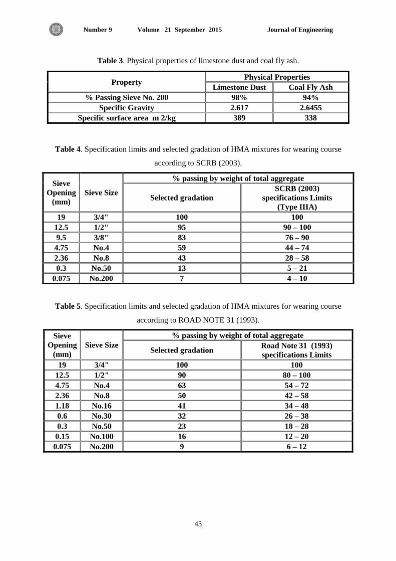
Table 3. Physical properties of limestone dust and coal fly ash.
Table 4. Specification limits and selected gradation of HMA mixtures for wearing course
according to SCRB (2003).
Sieve
Opening
(mm)
Sieve Size
% passing by weight of total aggregate
Selected gradation
SCRB (2003)
specifications Limits
(Type IIIA)
19 3/4" 100 100
12.5 1/2" 95 90 – 100
9.5 3/8" 83 76 – 90
4.75 No.4 59 44 – 74
2.36 No.8 43 28 – 58
0.3 No.50 13 5 – 21
0.075 No.200 7 4 – 10
Table 5. Specification limits and selected gradation of HMA mixtures for wearing course
according to ROAD NOTE 31 (1993).
Sieve
Opening
(mm)
Sieve Size
% passing by weight of total aggregate
Selected gradation Road Note 31 (1993)
specifications Limits
19 3/4" 100 100
12.5 1/2" 90 80 – 100
4.75 No.4 63 54 – 72
2.36 No.8 50 42 – 58
1.18 No.16 41 34 – 48
0.6 No.30 32 26 – 38
0.3 No.50 23 18 – 28
0.15 No.100 16 12 – 20
0.075 No.200 9 6 – 12
Property Physical Properties
Limestone Dust Coal Fly Ash
% Passing Sieve No. 200 98% 94%
Specific Gravity 2.617 2.6455
Specific surface area m 2/kg 389 338
Journal of Engineering Volume 21 September 2015 Number 9
44
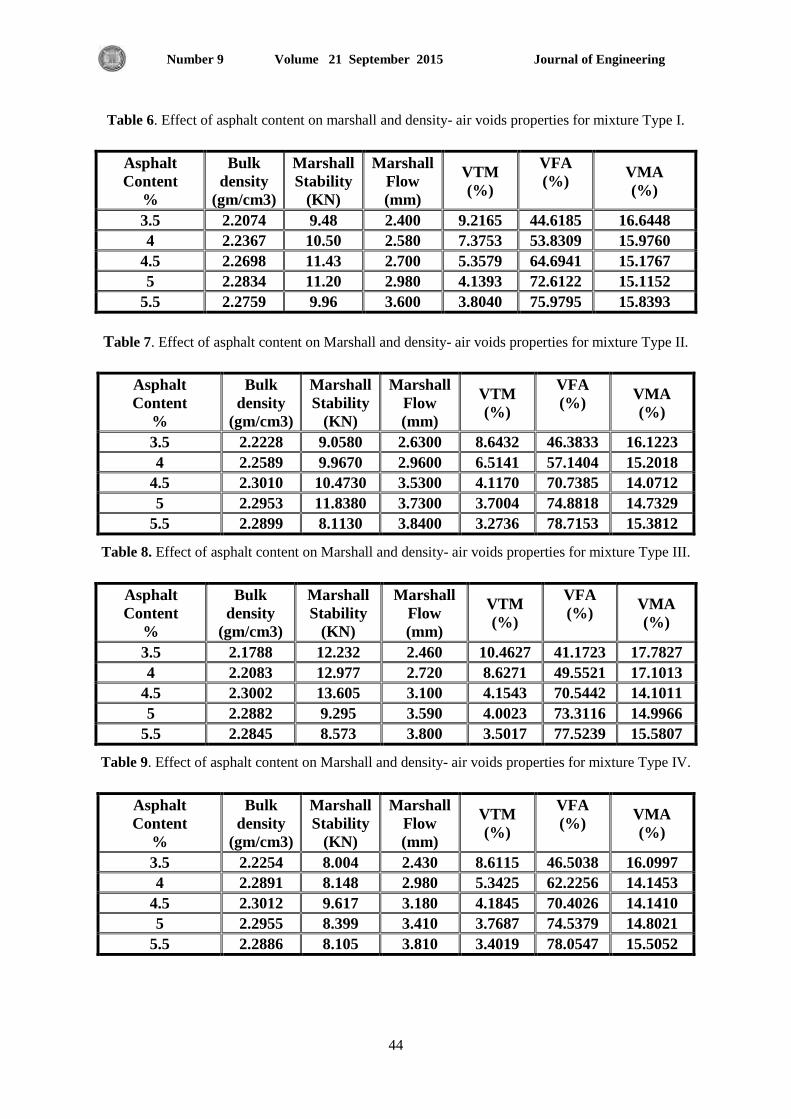
Table 6. Effect of asphalt content on marshall and density- air voids properties for mixture Type I.
Asphalt
Content
%
Bulk
density
(gm/cm3)
Marshall
Stability
(KN)
Marshall
Flow
(mm)
VTM
(%)
VFA
(%)
VMA
(%)
3.5 2.2074 9.48 2.400 9.2165 44.6185 16.6448
4 2.2367 10.50 2.580 7.3753 53.8309 15.9760
4.5 2.2698 11.43 2.700 5.3579 64.6941 15.1767
5 2.2834 11.20 2.980 4.1393 72.6122 15.1152
5.5 2.2759 9.96 3.600 3.8040 75.9795 15.8393
Table 7. Effect of asphalt content on Marshall and density- air voids properties for mixture Type II.
Asphalt
Content
%
Bulk
density
(gm/cm3)
Marshall
Stability
(KN)
Marshall
Flow
(mm)
VTM
(%)
VFA
(%)
VMA
(%)
3.5 2.2228 9.0580 2.6300 8.6432 46.3833 16.1223
4 2.2589 9.9670 2.9600 6.5141 57.1404 15.2018
4.5 2.3010 10.4730 3.5300 4.1170 70.7385 14.0712
5 2.2953 11.8380 3.7300 3.7004 74.8818 14.7329
5.5 2.2899 8.1130 3.8400 3.2736 78.7153 15.3812
Table 8. Effect of asphalt content on Marshall and density- air voids properties for mixture Type III.
Asphalt
Content
%
Bulk
density
(gm/cm3)
Marshall
Stability
(KN)
Marshall
Flow
(mm)
VTM
(%)
VFA
(%)
VMA
(%)
3.5 2.1788 12.232 2.460 10.4627 41.1723 17.7827
4 2.2083 12.977 2.720 8.6271 49.5521 17.1013
4.5 2.3002 13.605 3.100 4.1543 70.5442 14.1011
5 2.2882 9.295 3.590 4.0023 73.3116 14.9966
5.5 2.2845 8.573 3.800 3.5017 77.5239 15.5807
Table 9. Effect of asphalt content on Marshall and density- air voids properties for mixture Type IV.
Asphalt
Content
%
Bulk
density
(gm/cm3)
Marshall
Stability
(KN)
Marshall
Flow
(mm)
VTM
(%)
VFA
(%)
VMA
(%)
3.5 2.2254 8.004 2.430 8.6115 46.5038 16.0997
4 2.2891 8.148 2.980 5.3425 62.2256 14.1453
4.5 2.3012 9.617 3.180 4.1845 70.4026 14.1410
5 2.2955 8.399 3.410 3.7687 74.5379 14.8021
5.5 2.2886 8.105 3.810 3.4019 78.0547 15.5052
Journal of Engineering Volume 21 September 2015 Number 9
45
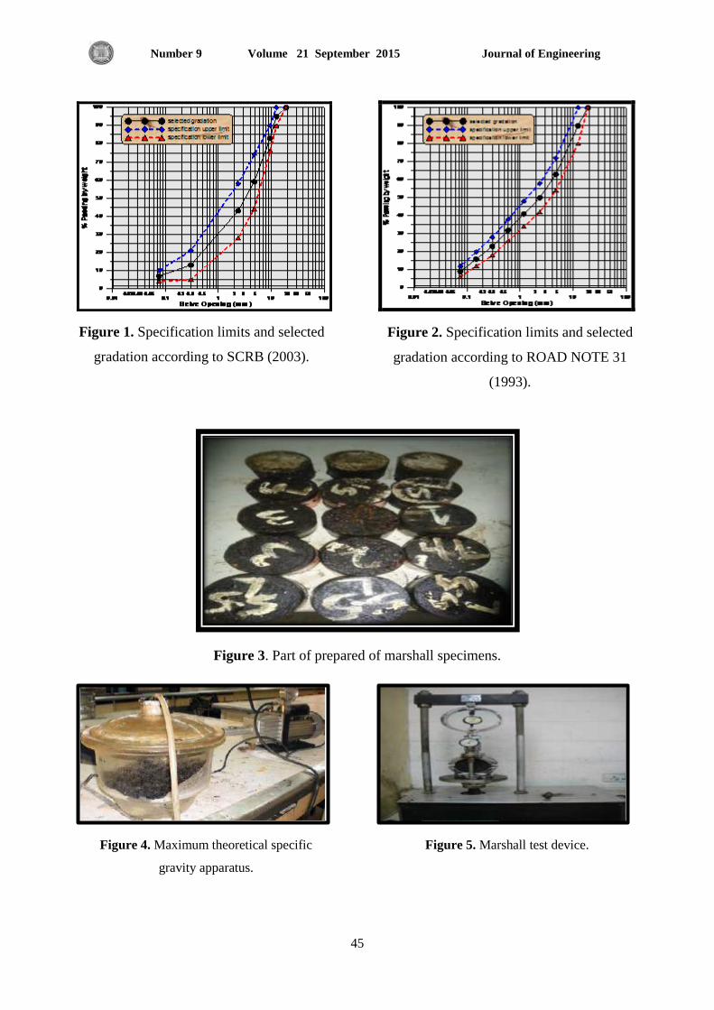
Figure 3. Part of prepared of marshall specimens.
Figure 1. Specification limits and selected
gradation according to SCRB (2003).
Figure 2. Specification limits and selected
gradation according to ROAD NOTE 31
(1993).
Figure 4. Maximum theoretical specific
gravity apparatus.
Figure 5. Marshall test device.

Journal of Engineering Volume 21 September 2015 Number 9
46
0
2
4
6
8
10
12
14
Type I Type II Type III Type IV
Stab
ility
KN
Mixture Type
0
0.5
1
1.5
2
2.5
3
3.5
4
Type I Type II Type III Type IV
Flo
w m
m
Mixture Type
2.27
2.275
2.28
2.285
2.29
2.295
2.3
2.305
Type I Type II Type III Type IV
Bu
lk d
en
sity
gm
/cm
^3
Mixture Type
3.6
3.7
3.8
3.9
4
4.1
4.2
4.3
Type I Type II Type III Type IV
V T
M %
Mixture Type
69
69.5
70
70.5
71
71.5
72
72.5
73
Type I Type II Type III Type IV
V F
A %
Mixture Type
13.6
13.8
14
14.2
14.4
14.6
14.8
15
15.2
15.4
Type I Type II Type III Type IV
V M
A %
Mixture Type
Figure 6. Effect of aggregate gradation and
filler type on Marshall stability.
Figure 7. Effect of aggregate gradation and
filler type on Marshall flow.
Figure 8. Effect of aggregate gradation and
filler type on bulk density.
Figure 9. Effect of aggregate gradation and
filler type on VTM.
Figure 10. Effect of aggregate gradation and
filler type on VFA.
Figure 11. Effect of aggregate gradation and
filler type on VMA.

Journal of Engineering Volume 21 September 2015 Number 9
16
Indoor Positioning and Monitoring System Using Smartphone and
WLAN (IPMS) Alaa Hamza Omran
M.Sc. Student College of Engineering - University of Baghdad
Email: [email protected]
Hamid Mohammed Ali
Assist Professor College of Engineering - University of Baghdad
Email: [email protected]
ABSTRACT Buildings such as malls, offices, airports and hospitals nowadays have become very complicated which increases the need for a solution that helps people to find their locations in these buildings. GPS or cell signals are commonly used for positioning in an outdoor environment and are not accurate in indoor environment. Smartphones are becoming a common presence in our daily life, also the existing infrastructure, the Wi-Fi access points, which is commonly available in most buildings, has motivated this work to build hybrid mechanism that combines the APs fingerprint together with smartphone barometer sensor readings, to accurately determine the user position inside building floor relative to well-known landmarks in the floor. Also the proposed system offers a monitoring activity which lets the administrator to watch and locate certain user inside the building.The system is tested in a big building indoor environment and achieved positioning accuracies of approximately 2.1 meters. Key words: Indoor Positioning System, Indoor Localization System, Indoor Monitoring System, Smart Phones, fingerprinting, Barometer sensor, WLAN, IPMS.
نظام مراقبو وتحذيذ مىقع الشخص داخل البنايو باستخذام الهاتف الذكي وشبكو لاسلكيو محليو
الاء حمزه عمران حامذ محمذ علي
طانث ياجستيش استار يساعذ جايع تغذاد –كهي انذس جايع تغذاد –كهي انذس
الخلاصةاطثذت انثاي يثم يشاكض انتسق انكاتة انطاسات انستشفيات في انلت انذاضش يعمذ نهغاي يايضيذ انذاج ان جد دم يساعذ اناط في ايجاد يلعى في ز انثاي. يعذ ظاو تذذيذ انالع انعاني اشاس اتشاج الاتظالات ادذ
اص خاسج تهك انثاي نكا نيست دليم في تذذيذ يالع الاشخاص داخم انثاي. ا انطشق انشائع في تذذيذ يالع الاشخجد اناتف انزكي في دياتا انييي تظس شائع كزنك تفش انثي انتذتي انمائ عه جد ماط انطل لذ دفض عه
ي اناتف انزكي نتذذيذ يلع انشخض تذل عه تاء ظاو جي يجع تظ ماط انطل يع لشاءات جاص الاستشعاسفانطاتك سث ان علاي يعشف في زا انطاتك. ايضا انظاو انمتشح يفش خاطي انشالث انتي تسخ نهششف تشاذ
انشخض ايجاد يلع شخض يعي داخم انثاي. لذ تى اختثاس انظاو في تاي كثيش ديث تهغت سث انذل في تذذيذ يلع يتش. 12,يايماسب
Journal of Engineering Volume 21 September 2015 Number 9
17
1. INTRODUCTION
Indoor positioning system recently has become an important topic in the research area due to the
growing demand for location aware systems that filter information based on the location of the
current smartphone. Many approaches, mechanisms, have been suggested and built for efficient
and accurate indoor positioning system. However, each of which comes with its merits and
demerits. GPS is the most widely used satellite based positioning system, which offers maximum
coverage. GPS cannot be deployed inside buildings, because it requires line-of-sight transmission
between receivers and satellites which is not possible in indoor environment due to the obstacles
inside the buildings, Hightower, and Borriello, 2001. Balas, 2011. presents a crowdsourcing-
based localization system for estimating the positions of the devices through using smartphone
sensor and Wi-Fi readings. However, the accuracy of this approach is approximately 7m which
decreases the performance of the system, furthermore, as mentioned in Balas, 2011. the number
of training data points has to be high in order to have a small error and people might not provide
this data whenever they are asked to by the phone. Most probably, the users will provide data
while in their offices or in the common areas and not while they are walking down the hallways.
Li, 2012. presents an indoor positioning system using smartphone sensors; this system interacts
with a user to get the initial location through user input, and provides the current position
estimate on an indoor map. However, smartphone sensor suffers from noises which makes
reliable step detection hard task, the random bouncing of mobile phones, caused by putting
phone in a pocket, switching from left to right hand, operating on touch screen, or taking a phone
call, can generate false positives in the detection; The step length of a person’s walking can vary
quite a lot over time, due to speed, terrain, and other environmental constraints. Furthermore, it is
well understood that people with different physical profiles such as height, weight, sex, or
walking style have different step length. In order to eliminate the challenges as mentioned above,
additional overhead and complexity are presented in the implementation algorithm. Kothari, et
al., 2012. present an indoor positioning system based on Wi-Fi Access Points incorporated with
smartphone sensor. However, it needs a pioneer robot equipped with a SICK LM200 laser
rangefinder for collecting signals from the APs during the process of APs detection which means
an additional hardware is needed results in increasing the complexity of implementation as well
as increasing the cost. Aboodi, and Wan, 2012. present an indoor positioning system based on
RSS fingerprint in conjunction with trilateration technique. However, using trilateration
technique imposes a constraint on the floor’s infrastructure because each floor should contain at
least three APs. Also, it uses LSE (Least Square Estimation), Min-Max and Kalman filter
algorithms which increases the complexity of the implementation as well as increasing in the
response time.
The rest of the paper is organized as follows. Section 2 describes in details the proposed system
mechanism. Section 3 describes the performance evaluation of the proposed system and provides
a comparison of indoor positioning techniques based on their accuracies. Finally, section 4
concludes the paper.

Journal of Engineering Volume 21 September 2015 Number 9
18
2. PROPOSED SYSTEM
This section logically illustrates the mechanism of the proposed system structure together with each
module that constructs the overall system architecture. The proposed system consists of two phases;
the training phase which is used to collect the strongest signal strength, of each AP, in each floor in
the building to be sent and stored in the database server. The localization phase is used to retrieve
the strongest signal strength from the database server then in conjunction with current smartphone
readings of AP signal strength and smartphone barometer are used to determine user position.
2.1 Training Phase
Fig. 1 shows the main components used in the training phase. The main function of the training
phase is to collect and record RSS of every AP, Pressure and height for each floor inside the site. In
this work the system is planned to work on a site which consists of a number of buildings each
building consists of a number of floors. Also each floor, which has its own pressure and height, is
equipped with one or more APs. Hence, each AP is identified by: site name, building name, floor
number, AP name, received signal strength (RSS), and AP MAC address. Before the training phase
starts, the system administrator smartphone is loaded with a utility that is responsible for collecting
the above mentioned information and then sent to be stored in the database server. Later In the
localization phase, these information in conjunction with information collected in real time, are
used to determine the local position of user. The steps that are involved in the training phase are
listed below:
1) The training phase utility is loaded in the system administrator smart phone and it is used only
during the training phase by the system administrator.
2) The site name is entered manually by the system administrator smartphone and sent to be stored
in the database server.
3) For each building, the system administrator walk through, the name of the building is entered
manually and sent to be stored in the database server.
4) For each floor, of each building, the floor number is entered manually and sent to be stored in
the database server.
5) Now for each floor while the administrator is walking through, the utility of the administrator
smartphone detects each AP and continuously read signal strength of each AP, as each AP is
recognized by its MAC address. When reaching to the end of the certain floor, the number of
recorded RSS for each AP is minimized at the Smartphone to the one of the strongest RSS
recorded for each AP; then, the strongest RSS of each AP is sent to be stored in database server.
Also, a well-known landmark such as common room in the floor, associated with each AP, is
also sent to be recorded in the database server. Note, the landmark should not be far away from
the AP more than one meter.
6) In addition, the utility of the administrator smartphone also detects the pressure, which is used
to calculate the height value, for each floor and send the height to be stored at the database
server. Note that, each floor has its own pressure and height values that are different from other
floors. The purpose of storing the height value, for each floor, will be explained and analysed in
the localization phase, section (2.2).
Fig. 2 shows the flowchart of the training phase for a building. Fig. 3 shows the Database entries.

Journal of Engineering Volume 21 September 2015 Number 9
19
2.2 Localization Phase Fig. 4 shows the main components used in the localization phase. This phase constitutes the main
objective of this paper which is responsible for providing “Locate Me” service, this phase
determines and notifies the user (through her/his smartphone) about her/his position relative to
well-known landmark inside the building. Also, it provides “Monitoring” service which lets the
administrator to locate certain users inside the building. Before discussing and analyzing the
technique and the approach used in this phase, it is found necessary to list the steps that would
clear the operation of different interoperated components:
A. Locate Me Service
1) While the user is walking inside the building, the “Locate Me” utility, embedded in the
smartphone, detects and reads the Wi-Fi RSS of the APs, pressure (for height calculations)
for the current floor and then compare them with retrieved RSS and height (which are stored
in the server during training phase), remember that each AP, in the building, is recognized by
site name, building name, floor number, AP’s name, RSS and its MAC address. Then a
mechanism called “Fingerprint Mechanism”, explained later in section (2.3) is used to
determine the closest AP (the one with strongest RSS) to the user and then it converts the
strongest RSS to a distance that represents how far the user is from the AP (landmark). Note
that, the purpose of extracting the height and pressure of each floor (using the smartphone
Barometer sensor) is: it happens that the detected closest AP to the user is in another floor,
actually not in the floor where the user exists. Hence the use of the pressure and height,
which are unique for each floor, will determine in which floor the user exists.
2) A “Filter Scheme” mechanism, shown in Fig. 4, is used to purify and removing the noise that
is associated with APs RSS and then determine the accurate and final position of the user to
be displayed on the user smartphone. The “Filter Scheme” mechanism is explained in details
later in section (2.5).
B. Monitoring Service
The monitoring service provides the administrator the capability of watching the users inside the
building. This service mainly depends on the “Locate Me” service. Thus whenever the ” Locate
Me” service is activated then all the information regarding users position are periodically send
and stored in the database server to be accessed by the administrator for the purpose of
monitoring. This service is explained in section (2.4).
2.3 Fingerprint Mechanism
Finger print mechanism, is the process of storing information at the training phase to be retrieved
at any time during the localization phase. It is important to know there are two types of indoor
localization, vertical and horizontal indoor localizations, it is necessary to distinguish between
them as follows:
1) Vertical localization which is the process of estimating user’s location according to which
floor number the user exists.
2) Horizontal localization which is the process of estimating user’s location on the specific floor
relative to well-known landmark at this floor.

Journal of Engineering Volume 21 September 2015 Number 9
20
2.3.1 Vertical Localization A problem that exists with the Wi-Fi mechanism is the number of APs for a fingerprint can be
changed because of the nature of radio waves. Especially inside buildings, external factors like
moving object, open or closed doors, change the signal strengths of the APs. An AP that was
measured during the training phase might not be received during the localization phase and vice
versa. Therefore, to account for these changes in the environment, the proposed system depends
mainly on the Barometer sensor of the smartphone in the vertical localization.
The proposed system uses Wi-Fi signal strength and the smartphone Barometer sensor to
estimate vertical user’s location, which floor number the user may exist. Barometer sensor is
used to measure height (altitude) and pressure, note that pressure and height have different
values in each floor in a specific building.
In the localization phase, the Wi-Fi signals of the APs are detected by the user’s smartphone.
Then the MAC addresses of the APs, from which the signals are received by the smartphone, are
compared with MAC addresses of the retrieved AP signals (stored in the database server during
the training phase). Furthermore, the Barometer sensor reading, associated with each detected
AP, is retrieved from the database server to be compared with current Barometer sensor reading
to determine which APs are in the floor where the user exists.
It is important to note, the Barometer sensor reading is changing with time, suppose the
Barometer sensor has a height value equal to 150.5 m at 10 O’clock morning. This value will be
altered according to the change in the parameters: pressure, temperature and humidity. Thus, the
Barometer sensor will have different reading after an hour, changing in height may be increased
or decreased according to the parameters mentioned above. This problem results in producing
error when the localization phase occurs at time different from the time of the training phase.
The proposed system fixes this problem through storing the Barometer sensor reading at each
floor in the database server, during training phase, arranged from the first floor to the last floor of
a specific building. Now, during the localization phase, which must start at the first floor, the
reading of the Barometer sensor at the first floor is subtracted from the value of the Barometer
sensor of the first floor stored during training phase, the result represents the difference between
the two values. This difference represents a new value called “Reference Point”, the new value
added to the all Barometer sensor readings, of each floor, that are detected and stored at the
database server during the training phase. For example, suppose a building consists of three
floors:
Let = 150.5 at first floor, = 153 at second floor and
= 157 at the third floor, if Barometer sensor reading has values equal to
=164 at first floor, =167 at second floor and
= 170 at third floor. Then during the localization phase, the following
equations are applied:

Journal of Engineering Volume 21 September 2015 Number 9
21
Reference Point= - (1)
=164-150.5=13.5
= - Reference Point (2)
=164-13.5= 150.5 which is exactly 150.5, the training phase value of the first floor.
= -Reference Point (3)
= 167-13.5=153.5 which is approximate to 153, the training phase value of the second floor.
= -Reference Point (4)
= 170-13.5=156.5 which is approximate to 157, the training phase value of the third floor.
The above new Height Barometer localization values are stored in a temporary list, inside the
smartphone, and updated continuously while the user is moving inside the building. Actually,
the list is updated every 5 seconds, according to the above mentioned procedure, to eliminate
the problem of Barometer sensor readings variations in different times of the day. Actually, In
other words every 5 seconds a new Reference Point is calculated and the above mentioned
equations are applied again.
2.3.2 Horizontal Localization It is time now to determine the horizontal localization, suppose the following scenario:
After performing the training phase for the first floor, suppose there are four APs called A, B,
C, D and each one has its own RSS value; these values are listed in Table 1.
During the localization phase, the detected APs and their own RSS are listed in Table 2 which
illustrates that the user is closest to AP B which has strongest RSS. Now, to find the closest
AP to the user, the Euclidean distance rule shown in Eq. (5) is applied.
D=√ (5)
Where D represents Euclidean distance; represents received signal strength at training
phase; represents received signal strength at localization phase.
Note that, the standard form of the Euclidean equation as used in previous works, Navarro, et
al., 2011. and Grossmann, et al., 2008. includes summation symbol inside the square root see
Eq. (6):
D=√∑ (6)
Where D represents Euclidean distance; represents received signal strength at training
phase; represents received signal strength at localization phase; N is the number of the
APs. Actually, Eq. (6) is used in the environment where group of APs are collected together
to represent certain well-known landmark at the floor. This approach is prone to error due to

Journal of Engineering Volume 21 September 2015 Number 9
22
the fact, suppose each floor has a number of APs which are collected in four groups. During
positioning time the APs are detected in more than one group, as long as each group has a
specific well-known landmark, then in order to estimate the closest well-known landmark, Eq.
(6) is calculated for each group.
Therefore, the summation symbol is used in the process of calculation for each group; the
group which has the smallest D has the closet position to the well-known landmark. However,
whenever the number of matching APs is increased then D will be increased producing
erroneous and inaccurate results.
In our proposal, the idea of APs groups is not adopted, during the localization phase all the
APs of certain floor are detected and compared with corresponding retrieved APs. Therefore,
the Euclidean equation is modified through eliminating the summation symbol from the
equation. Hence the modified Euclidean equation is applied for the example of Table 2 as
follows:
D1=√ = 10
D2=√ = 5
D3=√ =20
D4=√ =40
It is clear that the smallest distance is D2 which means the user is closest to AP B. In order to
calculate the distance in meter that how far the user is from AP B, Eq. (7) is used.
=
(7)
= = 8m
Where , is the real distance that the user is far away from the well-known landmark.
Note, referring to, Park, 2007. Adchi, and LitePoint, 2014. most of the APs have a
maximum indoor range of 30m. Referring to Galias, et al., 2013. the minimum RSS level
received by smartphone is -110db. Therefore, Eq. (7) has a maximum range of 30m. Fig. 5
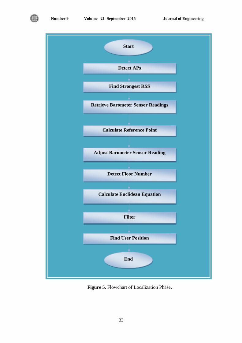
shows the flowchart of the localization phase, “Locate Me” service.
2.4 Monitoring Service
As mentioned in section (2.2), the localization phase offers “Monitoring” service for the
administrator to locate users inside the building. Actually, as long as the user position is
determined in “Locate Me” service, explained in section (2.3), then the “Monitoring”
service is smoothly accomplished according to the following steps:
1) As soon as activating the system by the user, the IPMS starts the process of finding user
position relative to the well-known land mark as explained in details in the “Locate Me”
service. In other words, user smartphone starts the process of finding user position without
user’s knowledge.

Journal of Engineering Volume 21 September 2015 Number 9
23
2) This information is associated with the username which is inserted by the user during the
process of system’s activation.
3) This information is uploaded to the database server.
4) The administrator can access the database server at any time and retrieve user position.
Note, the procedure of finding user’s position is repeated every 3 seconds which results in
updating user’s position every 3 to 5 seconds in the database server.
2.5 Filter Scheme Filter is used to purify the result of finding the closest AP based on Euclidean distance
algorithm. The idea is to make the algorithm so that the impact of large differences in RSS is
reduced, thus filter out the large differences so that if the RSS difference is larger than a
certain threshold, So, et al., 2013. the distance measure is no longer increased. Referring to
Eq. (4):
Let =C (8)
D=√ (9)
C= if | | ˂ TH (10)
C=TH if | | ≥ TH (11)
Where TH is the threshold value.
Now, in order to compensate the effect of some cases such as user orientation, user height,
how the user holds the smartphone, etc. RSS is shifted inside a certain range, So, et al., 2013.
D=√ (12)
Where z is the shift value.
According to So, et al., 2013, TH between range 10 to 30db and z in range between 3 to 10.
3. PERFORMANCE EVALUATION
This section demonstrates and illustrates the practical performance results that are obtained
from applying the proposed system in real environment; Al Mansour Mall building which
consists of four floors. The reason of applying the proposed system, in the above mentioned
site, is to have a test in vital place in real life which is crowded with people.
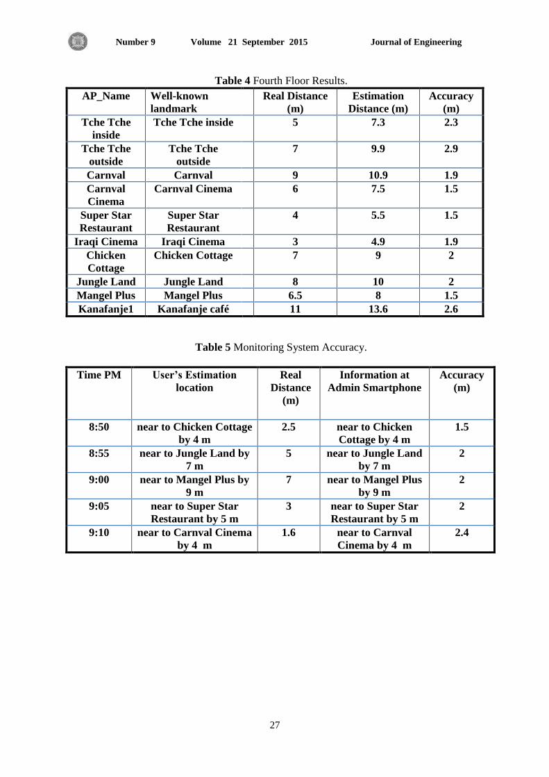
3.1 User Positioning System Testing
The training phase of Al Mansour Mall building is conducted for the entire building floors.
While the localization (positioning) phase is conducted in third and fourth floors, where five
locations were taken for the test in the third floor and ten locations are tested in the fourth
floor. Tables 3 and Table 4 show the results obtained from the test. From the results, the
proposed system achieved accuracy of approximately an average of 2.1m.
This section presents the results of testing the system from user point of view, in other words
if the user is lost inside the building it is simple to find her/his location using the positioning
system. Also suppose two friends lost each other inside crowded Mall; in this case each one

Journal of Engineering Volume 21 September 2015 Number 9
24
can find her/his location and send a text message to the other, using the positioning system, to
meet each other again.
3.2 User Monitoring System Testing
This section presents the results from the administrator point of view; in this test the user has
changed his location five times. Table 5 illustrates the location results recorded by the
administrator smartphone.
Accuracy (or location error) of a system is the important user requirement of positioning
systems. Accuracy can be reported as an error distance between the estimated location and the
actual mobile location. Sometimes, accuracy is also called the area of uncertainty; that is, the
higher the accuracy is, the better the system is. Some compromise between “suitable”
accuracy and other characteristics is needed. Table 6 shows system accuracies.
Note, the third system, shown in Table 6, achieves quite good accuracy of 2m which is nearly
equal to our proposal that achieves accuracy of an average of 2.1m. Actually, because this
system depends solely on the smartphone sensors suffers many challenges, some of them
mentioned in section 1and the others in Li, et al., 2012. which degrade system performance in
the long run of use.
The fifth system, shown in Table 6, also achieves quite good accuracy of 2.6m. But this
system depends solely on the Wi-Fi signals and because it uses complex mechanism, as
mentioned in section 1, which consumes a lot of computation time that results in slow
response time to the user.
4. CONCLUSION
A hybrid indoor positioning and monitoring system is built that integrates smartphone sensors
and Wi-Fi fingerprinting. The main advantage of this research is the creation of a system that
achieves the benefits of the flexibility, offering good coverage, user friendly, reducing the
complexity of the implementation as much as possible, having a reasonable cost and finally
producing high accuracy. The proposed IPMS is suitable for use at any time; using public
database server which makes the proposed system services available 24 hours a day. The
proposed IPMS depends on the APs of the building which are in turn produce building level
coverage. The proposed IPMS enhances the mechanism of using the well-known fingerprint
algorithm, K-nearest neighbor, for dealing with Wi-Fi signals during the training and
localization phases respectively. Furthermore, it enhances the Barometer sensor readings
which fix the problem of Barometer sensor readings variation with time. Finally, the proposed
IPMS is highly reasonable which provides good accuracy and consistent position information.
It was tested into two vital buildings; the results showed the average of accuracy of the
proposed IPMS is approximately 2.1m.
Actually, to achieve the above mentioned accuracy, each landmark has to be attached or
adjoined to corresponding AP. In case there is no familiar landmark attached to AP, then it is
possible to attach a simple landmark that illustrates the location of the AP relative well-known
landmark in the building floor.

Journal of Engineering Volume 21 September 2015 Number 9
25
REFERENCES
Aboodi, A., and Wan, T., 2012, Evaluation of Wi-Fi-based Indoor (WBI)
Positioning Algorithm, International Conference on Mobile, Ubiquitous, and
Intelligent Computing, IEEE.
Balas, C., 2011, Indoor Localization of Mobile Device for a Wireless Monitoring
System based on Crowdsourcing, M.sc Thesis, University of Edinburgh,
Edinburgh, United Kingdom.
Calis, G., et al., 2013, Analysis of the variability of RSSI values for active RFID-
based indoor applications, Turkish Journal of Engineering & Environmental
Sciences, Vol. 37, pp. 186-210.
Grossmann, U., et al., July 2008, RSSI-Based WLAN Indoor Positioning Within a
Digital Museum Guide, International Journal of Computing, Volume 7, Issue 2.
Hightower, J., and Borriello, G., 2001, Location systems for ubiquitous computing,
in Computer, vol. 34, pp. 57-66.
Kothari, N., et al., 2012, Robust Indoor Localization on a Commercial
Smartphone, Computer Science, Elsevier, Vol. 10, pp. 1114-1120.
Li, F. 2012, A Reliable and Accurate Indoor Localization Method Using Phone
Inertial Sensors, ACM.
LitePoint, 2013, IEEE 802.11ac: What Does it Mean for Test?, A tendy Company.
Navarro, E., Peuker, B., and Quan, M., 2011, Wi-Fi Localization Using RSSI
Fingerprinting, Computer Engineering, Child Development, California Polytechnic
State University, USA.
Park, Y., Adchi, F., 2007, Enhanced Radio Access Technologies for Next
Generation Mobile Communication, Spriger Sience and Business Media, ISBN
978-1-4020-5532-4.
So, J., et al., May, 2013, An Improved Location Estimation Method for Wi-Fi
Fingerprint-based Indoor Localization, International Journal of Software
Engineering and Its Applications, Vol. 7, No. 3.

Journal of Engineering Volume 21 September 2015 Number 9
26
Table 1. First Floor APs at Database Server.
Table 2 First Floor APs Detected during Localization Phase.
Table 3 Third Floor Results.
AP_Name RSS (db)
A -50
B -55
C -50
D -45
AP_Name RSS (db)
A -60
B -50
C -70
D -85
AP_Name Well-known
landmark
Real Distance (m) Estimation
Distance (m)
Accuracy
(m)
Barcelona
Cafe
Barcelona
Cafe
6 8.1 2.1
Barcelona
Café 1
Barcelona
Café
9 11 2
Clarks Clarks 5 7 2
Party 21 Party 7 8.9 1.9
Cosmetic Cosmetic 4 5.7 1.7
Journal of Engineering Volume 21 September 2015 Number 9
27
Table 4 Fourth Floor Results.
Table 5 Monitoring System Accuracy.
Time PM User’s Estimation
location
Real
Distance
(m)
Information at
Admin Smartphone
Accuracy
(m)
8:50 near to Chicken Cottage
by 4 m
2.5
near to Chicken
Cottage by 4 m
1.5
8:55 near to Jungle Land by
7 m
5 near to Jungle Land
by 7 m
2
9:00 near to Mangel Plus by
9 m
7 near to Mangel Plus
by 9 m
2
9:05 near to Super Star
Restaurant by 5 m
3 near to Super Star
Restaurant by 5 m
2
9:10 near to Carnval Cinema
by 4 m
1.6
near to Carnval
Cinema by 4 m
2.4
AP_Name Well-known
landmark
Real Distance
(m)
Estimation
Distance (m)
Accuracy
(m)
Tche Tche
inside
Tche Tche inside 5 7.3 2.3
Tche Tche
outside
Tche Tche
outside
7 9.9 2.9
Carnval Carnval 9 10.9 1.9
Carnval
Cinema
Carnval Cinema 6 7.5 1.5
Super Star
Restaurant
Super Star
Restaurant
4 5.5 1.5
Iraqi Cinema Iraqi Cinema 3 4.9 1.9
Chicken
Cottage
Chicken Cottage 7 9 2
Jungle Land Jungle Land 8 10 2
Mangel Plus Mangel Plus 6.5 8 1.5
Kanafanje1 Kanafanje café 11 13.6 2.6

Journal of Engineering Volume 21 September 2015 Number 9
28
Table 6 System Accuracies.
System Accuracy(m)
Global Positioning System (GPS), Hightower, and Borriello, 2001. 10
Indoor Localization of Mobile Device for a Wireless Monitoring
System based on Crowdsourcing, Balas, 2011.
7
A Reliable and Accurate Indoor Localization Method Using Phone
Inertial Sensors, Li, 2012.
2
Robust Indoor Localization on a Commercial Smartphone, Kothari, et
al., 2012.
5
Evaluation of Wi-Fi-based Indoor (WBI) Positioning Algorithm,
Aboodi, and Wan, 2012.
2.6
The Proposed System. ≈2.1

Journal of Engineering Volume 21 September 2015 Number 9
29
Figure 1 .Training Phase.

Journal of Engineering Volume 21 September 2015 Number 9
30
Start
Enter Site Name
Enter Building Name
Enter Floor Number
Read Barometer Sensor
Start Scan
End Scan
Choose the Strongest RSS of each AP
Upload Data to the Server
Last Floor?
End
Figure 2. Flowchart of Training Phase.
No
Yes

Journal of Engineering Volume 21 September 2015 Number 9
31
Figure 3. Database Entries.

Journal of Engineering Volume 21 September 2015 Number 9
32
DB
Localization Algorithm
Smartphone’s Sensor
Figure 4. Localization Phase (Locate Me Service).
Filter Scheme
Journal of Engineering Volume 21 September 2015 Number 9
33
Start
Detect APs
Find Strongest RSS
Retrieve Barometer Sensor Readings
Detect Floor Number
Adjust Barometer Sensor Reading
Calculate Reference Point
Find User Position
Filter
Calculate Euclidean Equation
End
Figure 5. Flowchart of Localization Phase.

Journal of Engineering Volume 21 September 2015 Number 9
581
Study Effect of Central Rectangular Perforation on the Natural Convection
Heat Transfer in an Inclined Heated Flat Plate
Lect. Kadhum Audaa Jehhef
Department of Equipment and Machine
Institute of Technology, Middle Technical University
Email: [email protected]
ABSTRACT
Anumerical solutions is presented to investigate the effect of inclination angle (θ) ,
perforation ratio (m) and wall temperature of the plate (Tw) on the heat transfer in natural
convection from isothermal square flat plate up surface heated (with and without concentrated
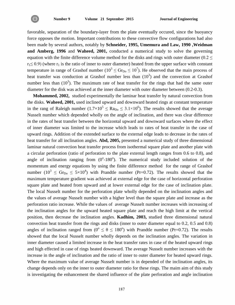
hole). The flat plate with dimensions of (128 mm) length × (64 mm) width has been used five with
square models of the flat plate that gave a rectangular perforation of (m=0.03, 0.06, 0.13, 0.25, 0.5).
The values of angle of inclination were (0o, 15
o 30
o 45
o 60
o) from horizontal position and the values
of wall temperature (50oC, 60
oC, 70
oC, 90
oC, 100
oC). To investigate the temperature, boundary
layer thickness and heat flux distributions; the numerical computation is carried out using a very
efficient integral method to solve the governing equation. The results show increase in the
temperature gradient with increase in the angle of inclination and the high gradient and high heat
transfer coefficients located in the external edges of the plate, for both cases: with and without
holed plate. There are two separation regions of heat transfer in the external edge and the internal
edges. The boundary layer thickness is small in the external edge and high in the center of the plate
and it decreases as the inclination angle of plate increases. Theoretical results are compared with
previous result and it is found that the Nusslet numbers in the present study are higher by (22 %)
than that in the previous studies. And the results show good agreement in range of Raleigh number
from 105 to 10
6.
Key words: natural convection, perforation plate, inclined flat plate.
يسخنة ر فوق صفيحة يائهةعهى انتقال انحرارة بانحم انحراري انحيركزي طيم يست تجويفتأثير دراسة
كاظى عودة جحفو.د.
قسى انكائ انعداخ
انعايعح انرقيح انسطى, تغداد -يعد ذكهظيا
انخلاصة
عهى ارقال انحرارج (Tw)درظح حرارج انسطح (m)سثح انرعيف (θ) زايح انيملاسرقصاء ذأشير دراسح عدديح قديد
يهفى( 528انصفييحح تطفل ) (يركفس يف تفد ذعيفف)تانحم انحر ي صفييحح يسفريح يرتعفح يسفمح يف انظف الاعهفى
يمرهيفففففح فففففاصض نهصفففففييحح انرتعفففففح يففففف شقفففففة يسفففففرطيم صاخ سفففففة ذعيفففففف خففففف ذفففففى اسفففففرمداو يهفففففى( 46) سففففف
0) ) ي ييم يمرهيح تسايا (m= 0.03, 0.06, 0.13, 0.25, 0.5)ي o, 15
o, 30
o, 45
o, 60
oدرظاخ قيى ي انض الافقي
50)حرارج يرغيرج ذرض oC, 60
oC, 70
oC, 90
oC, 100
oC) انطثقفح سف انحفرارج راسح ذزي كلا ي درظفح ي اظم د
فا اظفرخ انرفائط ا. انحاكفح انرياضفيحنركايم نحفم انعفادلاخ تاسرمداو انرحهيم انعدد تطريقح ا انييض انحرار انراخح
عايفم اعهفى قيفح ن . يرركس اعهى احفدار ففي درظفاخ حفرارجزايح انيم نهصييحححرارج ي زيادج اناحدار درظاخ في زيادج
ذرركفس لارقفال انحفرارج ل ايصفايطقرفي .ا (ي تد ذعيف)انحانري نكهراصييحح انحافاخ انمارظيح نهفي ارقال انحرارج
ففي انحاففح انمارظيفح قهيفم . نفحع ا سف انطثقفح انراخفح انحراريفح يكف انعففحصفييحح انمارظيفح نه انداخهيح في انحافاخ
دذف لاتانرفاق كهفا ازدادخ زايفح انفيذثفد ف انطثقفح في حانفح انفصض انمفاني يف ذعيفف. في يركس انصييححعاني
Journal of Engineering Volume 21 September 2015 Number 9
584
عا يظفد ففي انثحفز %(22 )د سهد في انثحس انحاني اعهى تسثح اعداظد ا انظريح انحانيح ي رائط ساتقح طرح انرائايق
10 ي في يد رقى رانيظيد تي انرائط ذقارب ظدانساتقح 510. انى
6
.ئهحصييحح يصقثح, صييحح يسريح يا : انحم انحر,نرئيسيهانكهات ا
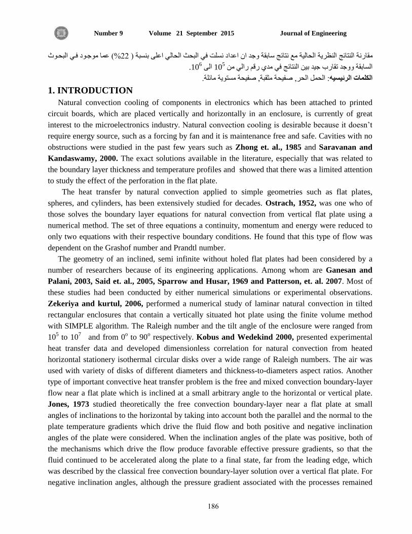
1. INTRODUCTION
Natural convection cooling of components in electronics which has been attached to printed
circuit boards, which are placed vertically and horizontally in an enclosure, is currently of great
interest to the microelectronics industry. Natural convection cooling is desirable because it doesn’t
require energy source, such as a forcing by fan and it is maintenance free and safe. Cavities with no
obstructions were studied in the past few years such as Zhong et. al., 1985 and Saravanan and
Kandaswamy, 2000. The exact solutions available in the literature, especially that was related to
the boundary layer thickness and temperature profiles and showed that there was a limited attention
to study the effect of the perforation in the flat plate.
The heat transfer by natural convection applied to simple geometries such as flat plates,
spheres, and cylinders, has been extensively studied for decades. Ostrach, 1952, was one who of
those solves the boundary layer equations for natural convection from vertical flat plate using a
numerical method. The set of three equations a continuity, momentum and energy were reduced to
only two equations with their respective boundary conditions. He found that this type of flow was
dependent on the Grashof number and Prandtl number.
The geometry of an inclined, semi infinite without holed flat plates had been considered by a
number of researchers because of its engineering applications. Among whom are Ganesan and
Palani, 2003, Said et. al., 2005, Sparrow and Husar, 1969 and Patterson, et. al. 2007. Most of
these studies had been conducted by either numerical simulations or experimental observations.
Zekeriya and kurtul, 2006, performed a numerical study of laminar natural convection in tilted
rectangular enclosures that contain a vertically situated hot plate using the finite volume method
with SIMPLE algorithm. The Raleigh number and the tilt angle of the enclosure were ranged from
105 to 10
7 and from 0
o to 90
o respectively. Kobus and Wedekind 2000, presented experimental
heat transfer data and developed dimensionless correlation for natural convection from heated
horizontal stationery isothermal circular disks over a wide range of Raleigh numbers. The air was
used with variety of disks of different diameters and thickness-to-diameters aspect ratios. Another
type of important convective heat transfer problem is the free and mixed convection boundary-layer
flow near a flat plate which is inclined at a small arbitrary angle to the horizontal or vertical plate.
Jones, 1973 studied theoretically the free convection boundary-layer near a flat plate at small
angles of inclinations to the horizontal by taking into account both the parallel and the normal to the
plate temperature gradients which drive the fluid flow and both positive and negative inclination
angles of the plate were considered. When the inclination angles of the plate was positive, both of
the mechanisms which drive the flow produce favorable effective pressure gradients, so that the
fluid continued to be accelerated along the plate to a final state, far from the leading edge, which
was described by the classical free convection boundary-layer solution over a vertical flat plate. For
negative inclination angles, although the pressure gradient associated with the processes remained
Journal of Engineering Volume 21 September 2015 Number 9
581
favorable, separation of the boundary-layer from the plate eventually occured, since the buoyancy
force opposes the motion. Important contributions to these convective flow configurations had also
been made by several authors, notably by Schneider, 1995, Umemura and Law, 1990 ,Weidman
and Amberg, 1996 and Waheed, 2001, conducted a numerical study to solve the governing
equation with the finite difference volume method for the disks and rings with outer diameter (0.2 ≤
r1≤ 0.9) (where r1 is the ratio of inner to outer diameter) heated from the upper surface with constant
temperature in range of Grashof number (103 ≤ GrDo ≤ 10
7). He observed that the main process of
heat transfer was conduction at Grashof number less than (103) and the convection at Grashof
number less than (103). The maximum rate of heat transfer for the rings that had the same outer
diameter for the disk was achieved at the inner diameter with outer diameter between (0.2-0.3).
Mohammed, 2002, studied experimentally the laminar heat transfer by natural convection from
the disks. Waheed, 2001, used inclined upward and downward heated rings at constant temperature
in the rang of Raleigh number (1.7×10⁵ ≤ RaDo ≤ 3.1×10
6). The results showed that the average
Nusselt number which depended wholly on the angle of inclination, and there was clear difference
in the rates of heat transfer between the horizontal upward and downward surfaces where the effect
of inner diameter was limited to the increase which leads to rates of heat transfer in the case of
upward rings. Addition of the extended surface to the external edge leads to decrease in the rates of
heat transfer for all inclination angles. Abd, 2005, presented a numerical study of three dimensional
laminar natural convection heat transfer process from isothermal square plate and another plate with
a circular perforation (ratio of perforation to the plate external length ranges from 0.6 to 0.8), and
angle of inclination ranging from (0o-180
o). The numerical study included solution of the
momentum and energy equations by using the finite difference method for the range of Grashof
number (103 ≤ GrDo ≤ 5×10
4) with Prandtle number (Pr=0.72). The results showed that the
maximum temperature gradient was achieved at external edge for the case of horizontal perforation
square plate and heated from upward and at lower external edge for the case of inclination plate.
The local Nusselt number for the perforation plate wholly depended on the inclination angles and
the values of average Nusselt number with a higher level than the square plate and increase as the
perforation ratio increase. While the values of average Nusselt number increases with increasing of
the inclination angles for the upward heated square plate and reach the high limit at the vertical
position, then decrease the inclination angles. Kadhim, 2003, studied three dimensional natural
convection heat transfer from the rings and disks (inner to outer diameter equal to 0.2, 0.5 and 0.8)
angles of inclination ranged from (0o ≤ θ ≤ 180
o) with Prandtle number (Pr=0.72). The results
showed that the local Nusselt number wholly depends on the inclination angles. The variation in
inner diameter caused a limited increase in the heat transfer rates in case of the heated upward rings
and high effected in case of rings heated downward. The average Nusselt number increases with the
increase in the angle of inclination and the ratio of inner to outer diameter for heated upward rings.
Where the maximum value of average Nusselt number is in depended of the inclination angles, its
change depends only on the inner to outer diameter ratio for these rings. The maim aim of this study
is investigating the enhancement the shared influence of the plate perforation and angle inclination

Journal of Engineering Volume 21 September 2015 Number 9
588
on the natural convection heat transfer process by using the numerical computation carried out
using the integral method to solve the governing equation and compare the theoretical result with
those of the previous studies.
2. PHYSICAL MODELS AND MATHEMATICAL FORMULATION
Consider the steady free convection flow of a viscous incompressible fluid over an inclined semi-
infinite plate at an angle ( ), as shown in Fig. 1. The temperature of plate is assumed constant at (Tw)
and the ambient fluid has the uniform temperature T∞, where Tw > T∞. For this configuration, the
assumption is that the Boussinesq approximation is valid ,Ioan 2001.
Figure 1. Physical models and coordinate systems of the heated inclined flat plate.
The body force by unit volume is –ρ g sin ( ), where g is the local acceleration of gravity. And
the key assumptions are:
1) Constant properties (ρ, k, Cp), except for the variation in density that drives the flow
2) Pressure gradients perpendicular to the plate can be neglected.
3) Density variation can be approximated by a linear dependence on temperature. This is called
the Boussinesq approximation.
4) Diffusive transport (of both momentum and energy) in the direction parallel to the plate can be
neglected. There are also, of course, many other implied assumptions (steady-state situation,
viscous dissipation is negligible in the energy equation, everything is constant in the z-
direction (parallel to plate, perpendicular to gravity)).
First, will be look up the “general” governing equations in a reference text, to find the following
equations. Any terms involving the z coordinate or the corresponding velocity component, can be
neglected as well as the transient terms. This leaves: Rolando, 2004, the basic conservation Eqs. (1),
(2) and (3) can be written as follows:
Continuity equation (overall mass balance)
0)()(
y
uv
x
uu
(1)
and momentum balance in x direction (parallel to plate and gravity) for a Newtonian fluid with
constant and .

Journal of Engineering Volume 21 September 2015 Number 9
588
)sin(2
2
2
2
gy
u
x
u
x
P
y
uv
x
uu
t
u
(2)
For a horizontal flat plate, the energy balance for a Newtonian fluid with constant and equation
reduces to,
2
2
y
T
y
Tv
x
Tu
(3)
where
0
t
u
2
2
2
2
y
u
x
u
Then, Eq. (2) becomes:
)sin(2
2
gy
u
x
P
y
uv
x
uu
(4)
singx
P
(5)
where is the density outside the boundary layer. Replacing Eq. (5) in Eq. (4) yields
2
2
))(sin(y
ug
y
uv
x
uu (6)
The first term on the right-hand side of Eq. (6) is the buoyancy force, where the density ρ is a
variable. The density may be represented by a linear function of temperature for small temperature
differences and the change in density is related to the thermal expansion, β, as: Rolando, 2004,
PT
1 (7)
If β is approximated by:
TT
1 (8)
then
)( TT (9)
and Eq. (2) becomes ,Rolando, 2004:
2
2
)()(siny
uTTg
y
uv
x
uu
(10)
hence, the buoyancy force is related to the temperature difference.

Journal of Engineering Volume 21 September 2015 Number 9
581
Momentum integral method is approximate and much easier to apply to a wide range of
problems than any exact method of solution. The idea behind this: is it is not really interest in the
detailing of the velocity or temperature profiles beyond learning their slopes at the wall (John,
2004). [These slopes give the shear stress at the wall is 0)( yw yu and the heat flux at the
wall is 0)( yw yTkq Schlichting, 1979, where the boundary conditions are:
T = Tw at y = 0
T = T∞ for y » ∞
u = v = 0 at y = 0
u = v = 0 for y » ∞
If the integral method is applied in Eqs. (10 and 3), these equations (momentum and energy
equations) will be respectively,John, 2004:
000
2 )(
yy
udyTTgdyu
dx
d
(11)
00
)(
yy
TdyTTu
dx
d
(12)
The functional forms are assumed as follows ,John, 2004 2
1 )1( uu (13)
and
2)1(
TT
TT
W
(14)
The first derivative of this equation with respect to (y) will be ,John, 2004
)(2
0
TT
y
Tw
y
(15)
where
y
After the first derivative of Eq. (13) is used and equaled to zero in order to obtain the value of
maximum velocity component termed u1 substituting this equation with Eq. (15) into Eq. (11) gives
the general solution of the laminar thermal boundary layer without pressure gradient
4
1
2
1
4
1
)()(]952.0[93.3
xGrprprx
(16)
the Grx is the local Grashof number
2
3)()sin(
xTTgGr W
x
where ( ) is the inclination angle of flat plate with horizontal position.
The solution of the boundary-layer equations for any convection heat transfer problem gives
the velocity and temperature distributions. This is true for any type of solution (analytical or
numerical) and for any type of convection (forced or natural). Once the solution is obtained, the
heat-transfer coefficient is obtained by realizing that as we approach the solid surface, the velocity
vector is tangent to the surface and the heat-flux vector is normal to the surface, thus the heat
transfer is by conduction at the limit as the distance from the wall approaches zero. Therefore, for
the problem described in the previous section, the heat flux is:

Journal of Engineering Volume 21 September 2015 Number 9
585
0
)(
y
wy
TkTThq (17)
Subtracting into Eq. (17), will give:
2
k
h
The value of from Eq. (16) is used to get the local heat transfer coefficient along the length
of flat plate with respect to x component as follows:
4
1
4
1
4
1
2
1
)(]952.0[)(508.0
xGrkprprh xx (18)
The Nusselt number is found from the following relation:
k
xhNu x
x (19)
The heat dissipation from the heated flat plate can be determined from the following relation:
)( WTThAQ (20)
3. PROBLEM DEFINITION In natural or free convective heat transfer, heat is transferred between a solid surface and a fluid
moving over it, where the fluid motion is entirely caused by the buoyancy forces arising from density
changes that result from the temperature variations in the fluid, this motion is called natural convection
which can be either laminar or turbulent. However, because of the low velocities that usually exist in
natural convection, laminar flow occurs more frequently than turbulent flow. In this paper, attention is
therefore focused on two dimensional laminar natural convective flow. If the temperature differences
are small enough, the fluid properties, except the fluid density, may be assumed to be constant (fluid
density can not be assumed constant, because its variation induces the fluid motion).
In the present work a heated aluminum flat plate is used with dimensions of (128mm length ×
64mm width) and additionally five models of central perforation are used heated from upward flat plate
with dimension of rectangular perforates dimensions of (2mm×4mm), (4mm×8mm), (8mm×16mm),
(16mm×32mm) and (32mm×64mm) are represented by the ratio of the flat plate length to the
perforation length of (m=0.03, 0.06, 0.13, 0.25 and 0.5) respectively. The constant wall temperatures
used in this search were (50oC, 60
oC, 70
oC, 90
oC, 100
oC). Fig. 2 illustrates the flat plate with and
without central perforation and shows the perforation length.
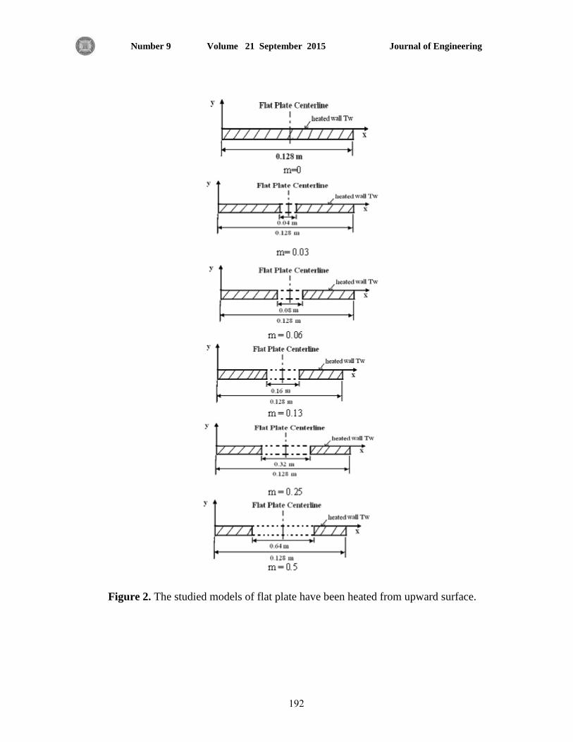
Journal of Engineering Volume 21 September 2015 Number 9
582
Figure 2. The studied models of flat plate have been heated from upward surface.

Journal of Engineering Volume 21 September 2015 Number 9
581
4. RESULTS AND DISCUSSION
The figures in this paper were generated by the (MATLAB 7) simulation program to study the
effect of the five central rectangular perforations in the heated upward flat plate. Figs. 3 and 4 show
the relationship between the distribution of dimensionless wall temperatures gradient and the region
above the flat plate represented by y-direction for the model of heated upward rectangle flat plate
without perforation (m=0) for values along the x-direction ranging as follows (x/Lo =1, 0.75, 0.5,
0.25, 0.15, 0.06 and 0.03) at horizontal position (θ=0o). The results compared with the results of the
model (m=0.13) for range of values along the x-direction (x/Lo =1, 0.75, 0.5, 0.25) at the same
position (θ=0o). The numerical data shows that central perforation is used in the plate in order to
avoid entering the slight declination region. The temperature gradients were located at positions
(x/Lo = 0.03, 0.06 and 0.15) in the range of the central perforation. The figures show that high
temperatures gradient along y-direction is achieved for the all models at the external edge while the
low temperatures gradient exists at the internal edge of perforation models and increases with
increasing the perforation ratio. And Fig. 5 shows the development of the thermal boundary layer
thickness (δ) along the x-direction of the heated flat plate for various value of the wall temperature
(50oC, 60
oC, 70
oC, 90
oC, 100
oC) for two selected models of (m=0 and 0.13) respectively at
horizontal position (θ=0o). As is shown in these figures, the thermal boundary layer thickness (δ) is
low at the external edge and increases gradually towards the flat plate center, because the fluid
molecular density near the models edges is higher than that near the center with high velocity
leading to generate the Plume ( the thermal separation happens). As a result the thermal boundary
layer thickness (δ) increases at the center more than at edges. The transmitted heat at the thermal
separation region will be less than that at the external edge.
Fig. 6 shows the development of thermal boundary layer along x-axis for various values of wall
temperature for the model of heated flat plate (m= 0.13). It is noticed that the thickness of thermal
boundary layer increases gradually from the edge of flat plate towards the center and decreases as
the wall temperature increases. in comparison with the model (m= 0.13) in Fig.5 which shows in
that the thickness of boundary layer is interrupted in the edge at (x=0.056 m) while in the
centerline of flat plate at (x=0.064 m), the boundary layer thickness increases from the external
edges towered the internal edge in which the thickness decreases with increase in the perforation
ratio, compared with first model (m=0) show that the thickness of boundary layer decreases with
increasing the perforation ratio because of the increase in the temperature gradient at the internal
edges.
Figs. 7 and 8 present the effect of flat plate inclination angle on the thermal boundary layer
thickness for two models of the heated plate (m= 0) and (m= 0.13). As shown in these figures, the
thermal boundary layer decreases as the angle inclination deviates from horizontal towards inclined

Journal of Engineering Volume 21 September 2015 Number 9
586
position because increasing the temperatures gradient, Abd 2005. Eventually; the effect of all
models of upward heated flat plate on the dimensionless wall temperature gradients (φ) with y-
direction are collected in Fig. 9 that shows the increasing the dimension of the central perforation
from (m=0 and 0.06) leads to increasing the dimensionless wall temperature gradients, then this
increase goes down when the model (m=0.5) is used because the high area removed from the flat
plat leading to decreasing the wall temperature distribution exposed to the ambient.
The local heat transfer coefficient hLo at horizontal position (θ=0o) of two models of heated
plate (m= 0) and (m= 0.13) is shown in Fig. 10 the maximum values are achieved in the external
edge because of the movement of the thermal boundary layer, and the heat separation at this
location of the flat plate. The local heat transfer coefficients decrease gradually from the edge of the
flat plate towards the center and the minimum values are at centerline, where the local heat transfer
coefficients increase as the wall temperatures increases. The effect of using perforation model of
(m=0.13) shown in Fig. 11. There are two regions of the heat separation along the upper surface of
heated flat plate: the first one exists in the external edge (x=0) of the plate because this edge is
adjacent to the infinity medium and the second one at (x=0.056) near the perforation internal edge
because this edge is adjacent to the finite medium. Fig. 12 shows the effect of perforation ratio on
the local Nusselt numbers for all models (m=0, 0.03, 0.06, 0.13, 0.25 and 0.5) with x-direction at
horizontal position (θ=0o) the figure shows that the high value of local Nusselt numbers is located
in the external edge of the heated flat plate and at perforation edge, The local Nusselt numbers
increase as the perforation dimension increases and show that the model (m=0.5) shows high value
of Nusselt numbers compared with other models.
Fig. 13 shows the relation between the logarithmic local Nusselt numbers with the algorithm of
the local Raleigh numbers (1.5×10⁵ ≤ Rax ≤ 6.3×10
5) at horizontal position (θ=0
o), where the
logarithm local Nusselt numbers increase as the perforation ratio increases, because by using the
perforation technique, the extraction of the thermal separation region centric in the central of the
plate. And when the inclination angles increase to (θ=30o) as in Fig. 14 the relation between the
logarithm of the local Nusslet numbers and the algorithm of the local Raleigh numbers (1.01×10⁵ ≤
Rax ≤ 6.4×10⁵) for the all models, show that the local Nusslet numbers increase as the perforation
dimensions and the angle of inclination increase, and the high local Nusselt numbers of (Nu =0.761
Ra 0.201
) of the model (m=0) and (Nu =0.985 Ra0.211
) of the model (m=0.13) where the perforation
dimensions are (8mm×16mm) at inclination of angle of (30o) and the increasing ratio between
(m=0) and (m=0.13) is (23%) .
A comparison of average Nusselt numbers for the square plate in present study with those of the
previous practical and numerical studies on the horizontal square heated plate for, Abd 2005
illustrated in Fig. 15 which shows the average Nusselt numbers for the present study at angle of
inclination (θ =0o) with no central perforation of model (m=0) increasing by (15 %). in the other

Journal of Engineering Volume 21 September 2015 Number 9
581
hand, the results are compared with those of the previous studies which used horizontal heated disk
for Abd, 2005, Mohammed, 2002 and Kadhim, 2003 as shown in Fig. 16 which shows that the
average Nusselt numbers agreement with the value studied by them. And at Raleigh number 1.47
×105 the model (m=0.5) shows that Nusselt numbers in the present study compared with those in
the previous studies give an increase of about (20.3%), (22.6%) and (22.1 %) for the results of
Abd, 2005, Mohammed, 2002 and Kadhim, 2003 respectively. This study show a good agreement
in terms of the Nusselt numbers for the heated upward plate at angle of inclination (φ =30o) with
central perforation of model (m=0.25) compared with the square plate perforated with the circular
perforation of Abd, 2005 and rings of the,Mohammed. 2002.
6. CONCLUSIONS
A numerical investigation was carried out to study the natural convection heat transfer in the
rectangular upward heated inclined perforated flat plate. In this paper, the influence of perforation
ratio (m), Raleigh number (Ra), the angle of inclination (θ) and wall temperatures (Tw) were
investigated. The numerical results show that: (1) the thermal boundary layer thickness increases as
the wall temperature increases and as the angle of inclination decreases (2) The maximum values of
local heat transfer coefficients are achieved at the leading edge of the flat plat for all models and at
any angle of inclination. (3) The heat transfer process is enhanced with the perforation dimension
increases. (4) The average Nusslet number for the present paper at angle of inclination (θ=0o) with
no central perforated perforation ratio (m=0) increases by (15 %). (5) The Nusselt number values
agree with these values presented by previous studies, with increase by (22 %) at (Ra=1.47 ×10⁵)
and (m=0.5).
REFERENCES
Abd Y.H. 2005, Numerical study for a three dimensional laminar natural convection heat
transfer from an isothermal heated horizontal and inclined square plate and with a circule
hole" M. Sc. Thesis University of Technology.
Ioan, L. M. 2001,Convective Heat Transfer: Mathematical and Computational Modeling of
Viscous Fluids and Porous Media. Elsevier Science & Technology Books.
Ganesan, P. & Palani, G. 2003, Natural convection effects on impulsively started inclined
plate with heat and mass transfer, Heat and Mass Transfer, 39, 277–283.
Jones, D. R. 1973. Free convection from a semi-infinite flat plate inclined at a small angle
to the horizontal. Q. J. Mech. Appl. Math. 26, 77-98.
John H. Lienhard 2004, A Heat Transfer Textbook" Mechanical Engineering. University of
Houston.

Journal of Engineering Volume 21 September 2015 Number 9
584
Kobus G.L and Wedekind R.O. 2000 , An experimental investigation into Natural
convection heat transfer from horizontal stationery isothermal circular disks Department of
Mechanical Engineering, Oakland University 5 May.
Kadhim A.H., 2003, Prediction of three dimensional natural convection from heated disks
and rings at constant temperature. J. Eng. and Technology. Vol.22, No.5, pp.229-248.
Mohammed J.A., 2002,. Measurement of three dimensional natural convection heat transfer
from disks and rings facing upward and downward at constant temperature M. Sc. Thesis
University of Baghdad.
Ostrach S., 1952. An Analysis of Laminar Free-Convection Flow and Heat Transfer
about a Flat Plate Parallel to the Direction of the Generating Body Force. Report 1111-
Supersedes NACA TN 2635.
Patterson J.C, Lei C. and. Saha S.C. 2007. On the Natural Convection Boundary Layer
Adjacent to an Inclined Flat Plate Subject to Ramp Heating School of Engineering James
Cook University, Townsville, QLD 4811, Australia December.
Umemura, A. and Law, C. K. 1990. Natural Convection Boundary-Layer Flow Over a
Heated Plate with Arbitrary Inclination. J. Fluid Mech. 219, 571-584.
Rolando A. Carrefio 2004, Natural Convection Heat Transfer in Supercritical Fluid
Mechanical Engineering University of Puerto Rico.
Saravanan S. and Kandaswamy P., 2000. Natural Convection in low Prandtl number Fluids
with a Vertical Magnetic Field, ASME J. Heat Transfer, 122, pp. 602–606.
Said, S. A. M., Habib, M. A., Badr, H. M. and Anwar, S. 2005. Turbulent Natural
Convection Between Inclined Isothermal Plates, Computers & Fluid, 34, 1025–1039.
Sparrow, E. M. and Husar, R. B., 1969. Longitudinal Vortices in Natural Convection Flow
on Inclined Plates , J. Fluid. Mech.37, , 251–255.
Schneider, W. 1995. Laminar Mixed Convection Flows on Horizontal Surfaces". In 3rd
,
Caribbean Congr. Fluid Dyn. Volume II, Simon Bolivar Univ., Caracas, pp. 1-7.
Schlichting H., 1979. Boundary Layer Theory, seventh edition translated by Kestin J.,
McGraw-Hill Book Company , new york.
Waheed A.M. 2001. Numerical and Experimental Study Natural Convection Heat Transfer
from Isothermal Horizontal Disks and Rings. M. Sc. Thesis University of Technology
Weidman, P. D. and Amberg, M. F. 1996. .Similarity Solutions for Steady Laminar
Convection Along Heated Plates with Variable Oblique Suction. Newtonian and Daxcian
fluid flow. Q. J. Mech. Appl. Math. 49,373-403.
Zhong Z.Y., Yang K. T., Lloyd J. R., 1985. Variable Property Effects in Laminer Natural
Convection in a Square Enclosure, ASME J. Heat Transfer, 17, pp. 133–138.
Zekeriya and kurtul 2006 Natural Convection in Tilted Rectangular Enclosures with a
Vertically Situated Hot Inside" Osmangazi University 7 July.

Journal of Engineering Volume 21 September 2015 Number 9
581
NOMENCLATURES
A area of the heated plate, m2
Nu average Nusselt number, --
p pressure, N/m2
g acceleration due to gravity, m/s2
t dimensional time, s
Gr Grashof number, ---
h average heat transfer coefficient, W/m2.oC
hx local heat transfer coefficient, W/m2.oC
u, v dimensional velocity components, m/s2
x, y dimensional coordinates, m
Nux local Nusselt number, ---
Pr Prandtl number, ---
m perforation ratio, ---
k thermal conductivity, W/m.oC
T predicted temperature
T∞ ambient temperature
Tw plate wall temperature
x
Greek Symbols
α thermal conductivity, m2/s
β volumetric coefficient of thermal expansion, 1/K
θ angle of inclination, degree
ρ density, kg/m3
δ boundary layer thickness, mm
ν kinematic viscosity, m2/s
μ absolute viscosity, kg/m.s
φ dimensionless temperature
ζ dimensionless viscosity

Journal of Engineering Volume 21 September 2015 Number 9
588
0
0.2
0.4
0.6
0.8
1
1.2
0 0.01 0.02 0.03 0.04 0.05 0.06 0.07
x/Lo=1
x/Lo=0.75
x/Lo=0.5
x/Lo=0.25
x/Lo=0.15
x/Lo=0.06
x/Lo=0.03
Figure 3. Dimensionless wall temperatures gradient vs. y-direction for the model of heated upward
rectangle flat plate without perforation (m=0) for range values along the x-direction at horizontal
position (θ=0o).
0
0.2
0.4
0.6
0.8
1
1.2
0 0.01 0.02 0.03 0.04 0.05 0.06 0.07
y (mm)
x/Lo=1
x/Lo=0.75
x/Lo=0.5
x/Lo=0.25
Figure 4. Dimensionless wall temperature gradients vs. y-direction for the model of heated upward
rectangle flat plate with central perforation of dimension of (16mm×32mm) (m=0.13) for range
values along the x-direction at horizontal position (θ=0o).
) T-(T
)T - (T
w
(mm)y
(mm)y
) T-(T
)T - (T
w
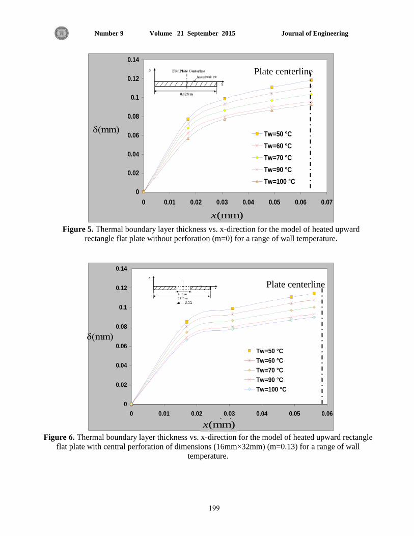
Journal of Engineering Volume 21 September 2015 Number 9
588
0
0.02
0.04
0.06
0.08
0.1
0.12
0.14
0 0.01 0.02 0.03 0.04 0.05 0.06 0.07
Tw=50 °C
Tw=60 °C
Tw=70 °C
Tw=90 °C
Tw=100 °C
Figure 5. Thermal boundary layer thickness vs. x-direction for the model of heated upward
rectangle flat plate without perforation (m=0) for a range of wall temperature.
0
0.02
0.04
0.06
0.08
0.1
0.12
0.14
0 0.01 0.02 0.03 0.04 0.05 0.06
Tw=50 °C
Tw=60 °C
Tw=70 °C
Tw=90 °C
Tw=100 °C
Figure 6. Thermal boundary layer thickness vs. x-direction for the model of heated upward rectangle
flat plate with central perforation of dimensions (16mm×32mm) (m=0.13) for a range of wall
temperature.
δ(mm)
Plate centerline
Plate centerline
δ(mm)
x (m) (mm)x
(mm)x

Journal of Engineering Volume 21 September 2015 Number 9
211
0
0.02
0.04
0.06
0.08
0.1
0.12
0.14
0.16
0.18
0 0.01 0.02 0.03 0.04 0.05 0.06 0.07
θ=0°
θ=15°
θ=30°
θ=45°
θ=60°
Figure 7. Thermal boundary layer thickness vs. x-direction for the model of heated upward
rectangle flat plate without perforation (m=0) for a range of inclination angles.
0
0.02
0.04
0.06
0.08
0.1
0.12
0.14
0.16
0.18
0 0.01 0.02 0.03 0.04 0.05 0.06 0.07
θ= 0°
θ=15°
θ=30°
θ=45°
θ=60°
Figure 8. Thermal boundary layer thickness vs. x-direction for the model of heated upward
rectangle flat plate with central perforation of dimensions (16mm×32mm) (m=0.13) for a range of
inclination angles.
Plate centerline
Plate centerline
δ(mm)
δ(mm)
(mm)x
(mm)x

Journal of Engineering Volume 21 September 2015 Number 9
215
0
0.2
0.4
0.6
0.8
1
1.2
0 0.01 0.02 0.03 0.04 0.05 0.06 0.07
m=0.13
m=0.25
m=0.5
m=0.06
m=0.03
m=0
Figure 9. Dimensionless wall temperatures gradient vs. y-direction for the all studied models of
heated upward rectangle flat plate.
0
2
4
6
8
10
12
14
16
0 0.01 0.02 0.03 0.04 0.05 0.06 0.07
Tw=50 °C
Tw=60 °C
Tw=70 °C
Tw=90 °C
Tw=100 °C
Figure 10. Local heat transfer coefficients vs. x-direction for the model of heated upward rectangle
flat plate without perforation (m=0) for a range of wall temperature at horizontal position (θ=0o).
hL
o (W
/m2.o
C)
Plate centerline
(mm)x
(mm)y
) T-(T
)T - (T
w
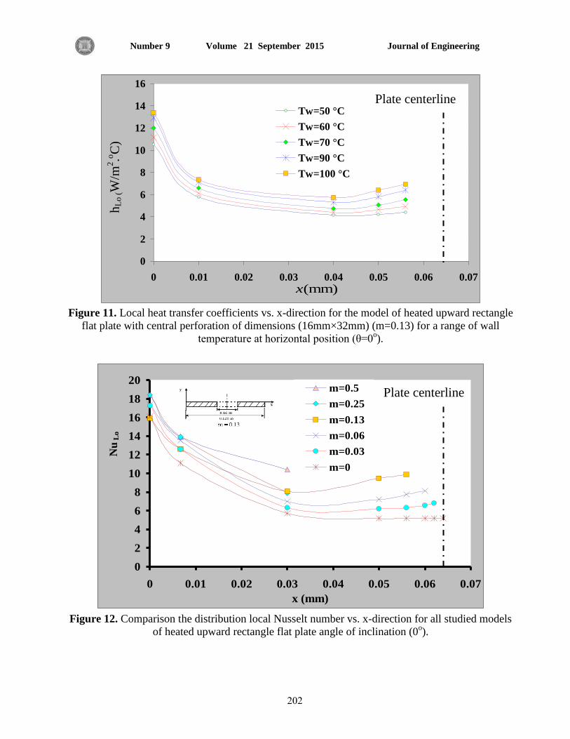
Journal of Engineering Volume 21 September 2015 Number 9
212
0
2
4
6
8
10
12
14
16
0 0.01 0.02 0.03 0.04 0.05 0.06 0.07
Tw=50 °C
Tw=60 °C
Tw=70 °C
Tw=90 °C
Tw=100 °C
Figure 11. Local heat transfer coefficients vs. x-direction for the model of heated upward rectangle
flat plate with central perforation of dimensions (16mm×32mm) (m=0.13) for a range of wall
temperature at horizontal position (θ=0o).
0
2
4
6
8
10
12
14
16
18
20
0 0.01 0.02 0.03 0.04 0.05 0.06 0.07
x (mm)
m=0.5
m=0.25
m=0.13
m=0.06
m=0.03
m=0
Figure 12. Comparison the distribution local Nusselt number vs. x-direction for all studied models
of heated upward rectangle flat plate angle of inclination (0o).
Plate centerline
Plate centerline
Nu
Lo
(mm)x
hL
o (W
/m2.o
C)
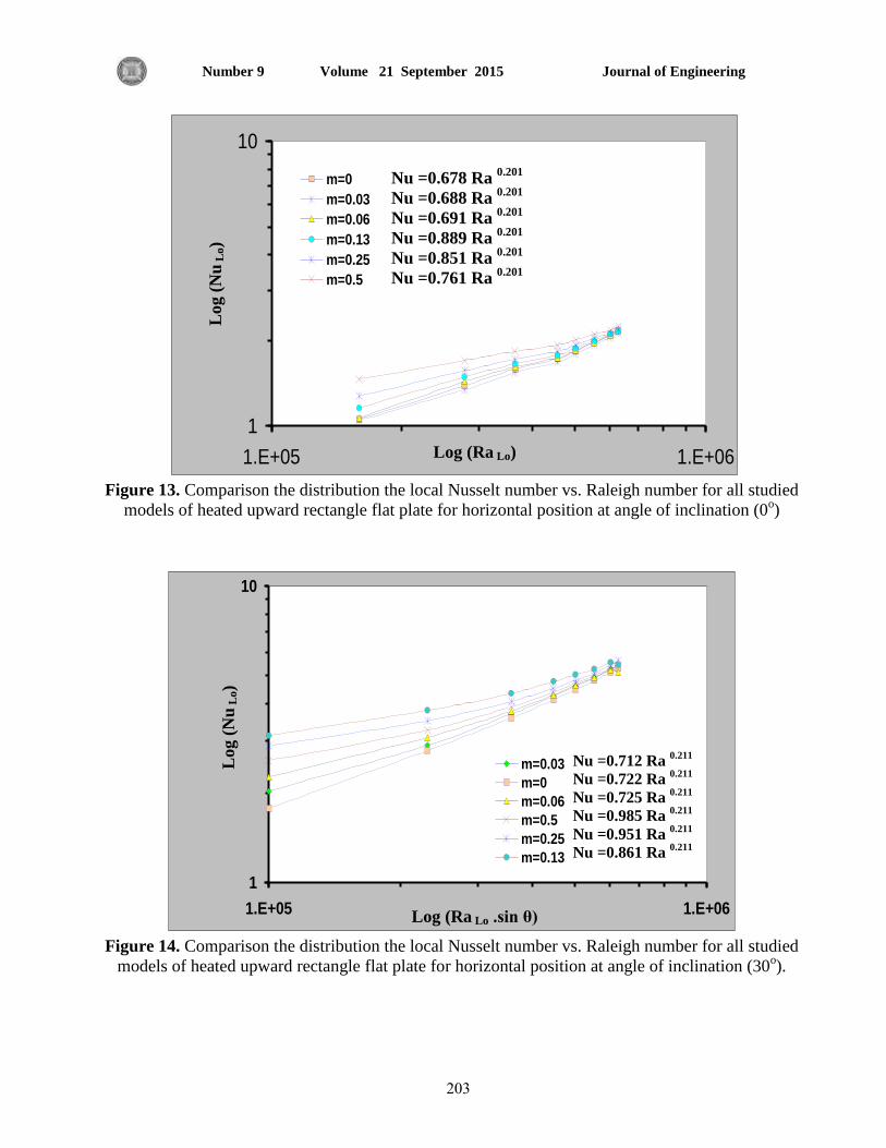
Journal of Engineering Volume 21 September 2015 Number 9
211
1
10
1.E+05 1.E+06
m=0
m=0.03
m=0.06
m=0.13
m=0.25
m=0.5
Figure 13. Comparison the distribution the local Nusselt number vs. Raleigh number for all studied
models of heated upward rectangle flat plate for horizontal position at angle of inclination (0o)
1
10
1.E+05 1.E+06
m=0.03
m=0
m=0.06
m=0.5
m=0.25
m=0.13
Figure 14. Comparison the distribution the local Nusselt number vs. Raleigh number for all studied
models of heated upward rectangle flat plate for horizontal position at angle of inclination (30o).
Log (Ra Lo)
Log (
Nu
Lo)
L
og (
Nu
Lo)
Log (Ra Lo .sin θ)
Nu =0.712 Ra 0.211
Nu =0.722 Ra 0.211
Nu =0.725 Ra 0.211
Nu =0.985 Ra 0.211
Nu =0.951 Ra 0.211
Nu =0.861 Ra 0.211
Nu =0.678 Ra 0.201
Nu =0.688 Ra 0.201
Nu =0.691 Ra 0.201
Nu =0.889 Ra 0.201
Nu =0.851 Ra 0.201
Nu =0.761 Ra 0.201

Journal of Engineering Volume 21 September 2015 Number 9
216
1
10
1.E+03 1.E+04 1.E+05 1.E+06
Present study (rectangular plate m=0)
Abd, 2005 (disk m=0)
Figure 15. Comparison of the distributions of the logarithm Nusselt number vs. Raleigh number
without perforation (m=0) heated upward rectangle flat plate for horizontal position at angle of
inclination (0o).
1
10
100
1.E+02 1.E+03 1.E+04 1.E+05 1.E+06
Mohammed, 2002 (Ring m=0.5)
Abd, 2005 (square plate with circle hole m=0.5)
Kadhim, 2003 (Disk with circle hole m=0.5)
Present study (rectangular plate m=0.5)
Figure 16. Comparison of the distribution of the local Nusselt number vs. Raleigh number with
perforation (m=0.5) heated upward rectangle flat plate for horizontal position at angle of inclination
(30o).
Log (
Nu
Lo)
Log (Ra Lo .sin θ)
Log (
Nu
Lo)
Log (Ra Lo .sin θ)

Journal of Engineering Volume 21 September 2015 Number 9
150
Dynamic Analysis of Fluid – Structure Interaction of Axial Fan System
Dr. Assim Hameed Yousif Dr. Wafa Abd Soud Aljanabi
Professor Instructor
Mechanical Engineering Department-University of Technology Mechanical Engineering Department-UOT
E-mail: [email protected] E-mail: [email protected]
Ali Mohammedridha Mahdi
Researcher
Mechanical Engineering Department-University of Technology
E-mail: [email protected]
ABSTRACT
Fluid-structure interaction method is performed to predict the dynamic characteristics of
axial fan system. A fluid-structure interface physical environment method (monolithic method) is
used to couple the fluid flow solver with the structural solver. The integration of the three-
dimensional Navier-Stokes equations is performed in the time Doman, simultaneously to the
integration of the three dimensional structural model. The aerodynamic loads are transfer from the
flow to structure and the coupling step is repeated within each time step, until the flow solution and
the structural solution have converged to yield a coupled solution of the aeroelastic set of equations.
Finite element method is applied to solve numerically the Navier-Stockes equations coupled with
the structural equations The first ten eigenvalue (natural frequency), the first ten eigenvector (mode
shape) and effective stress for each part of a rotor system and complete system assembly are
predicted.
The validity of the predicted dynamic characteristics of duct fan system was confirmed
experimentally by investigating geometrically similar fan system test rig. Good agreement of
dynamic characteristics is observed between experimental and numerical results.
Key words: dynamic, fluid-structure interaction, coupling strategies, fan system, natural frequency
and mode shape.
ل المائع والهيكل لمنظىمة مروحة محىريةتحليل ديناميكي لتذاخ
الجنابي وفاء عبذ سعىد د. عاصم حميذ يىسف د.
أسخبر ذسس
اىجبعت اىخنىجت - قس اىذست اىنبنت نىجتاىجبعت اىخ - قس اىذست اىنبنت علي محمذ رضا مهذي
اىببحث
اىخنىجتاىجبعت - اىنبنت قس اىذست
الخلاصةح سبظ اىحيه شحت حست. اسخخذج طشقت حذاخو جشب اىبئع اىنو ىيخبؤ ع اىزاب اىذبنت ىظت
.(monolithic method)ت اىبئت اىفزبئت ىخذاخو اىبئع اىنواىعذدت ىجشب اىبئع ع اىحيه اىعذدت ىينو ببسخخذا طشق
اىز طشقت اىخنبيت ثلاثت اىبعذ ع حيه عبدلاث اىنو اىخنبيت ثلاثت اىبعذ ببسخخذا سخك-حيه عبدلاث فش سبظح
ة ز اىخطة اىزدجت شاسا حنشاسا حخ حصو اىحذ. ىقذ ح قو الأحبه اىذبائت جشب اىبئع إى اىنو ح إعبد

Journal of Engineering Volume 21 September 2015 Number 9
151
الاىخئب اىنبو ىحيه عبدلاث اىجشب عبدلاث اىنو اىز قد إى حيه ىجعت عبدلاث اىشت اىفضبئت. ىقذ اسخخذج
ع عبدلاث ححيو اىنو. سخك( اىخ ححن اىبئع -طشقت اىعبصش اىحذدة لإجشاء اىحو اىعذد بشنو زدج ىعبدلاث )فش
ه عششة دبن لأ اجشاء ححيوح حذدة أجشاء اىخحيلاث اىطيبت.مب اسخخذج بشاجبث جبزة ىخشغو طشقت اىعبصش اى
الاجبداث اىفعبىت لأجزاء اىظت اىشئست فشدة ىيظت جخعت.مزىل حشدداث طبعت أه عششة إشنبه سق
حجشبب بئجشاء اخخببساث عيت صذاقخب اىخ ح اىخبؤ عب عذدب جش اىخأمذ اىشحت ىظتزاب اىذبنت إ اى
افق جذ ب . ىقذ ىحظ إ بك ححتىظت جش اىشحبم شنيب اىذس رج الاخخببس اىعذد عي صت فحص
بت ىيزاب اىذبنت ىيظت.خبئج اىقبسبث اىخجش خبئج اىخبؤ
1. INTRODUCTION
The implementation of a coupled problem (fluid-structure interaction) can be done by using
two different strategies, which are the monolithic methods and the partitioned method. In a
monolithic method, the discretized fluid-structure system is solved together with the mesh
movement system in a single iteration loop, leading to a very large system of nonlinear equations to
be solved simultaneously. Some advantages of this method are that it ensures stability and
convergence of the whole coupled problem. On the contrary, in simultaneous solution procedures
the time step has to be equal for all subsystems, which may be inefficient if different time scales are
presented for the problem. An important disadvantage is the considerable high computing time
effort required to solve each algebraic system and sometimes the necessity to develop new software
and solution methods for the coupling method. A monolithic approach to fluid-structure interaction
(FSI) used in the present work is introduced by Hübner, et al., 2004.
2. TEST RIG
The experimental test rig designed and manufactured according to the requirement of the
present study and its consists of driven motor, static frequency changers, spool shaft, fan, two
journal bearing, hollow shaft, eight probes, inlet bow mouth, mesh screen and duct casing. The
photograph of the test rig assembly and measuring instruments are shown in Fig. 1.
The spooled shaft is made from medium carbon steel (St 60.2), with tensile strength of
(600 – 720) N/mm², density (7840) Kg/m3, Young modulus (210) GN/m
2, modulus of elasticity
(80) GN/m2 and length (544.66) mm with step diameters along its length as shown in Fig. 2.
The purpose of using two bearings is to support the load to allow the relative motion being
smoothly between two elements of machine, made from porosity bronze alloy. Small holes (2 mm)
diameter are made into the bush to allow lubricant oil to pass between shafts and bush bearing to
lubricate the contact region and reduce temperature rise. The journal bearing oil film may be
idealized into stiffness and damping coefficients which affect the flexibility of the system and
introduce damping. The viscosity of the lubricant prevents journal bearing from escaping until
pressure is built up in the convergent–divergent film, forcing the lubricant oil to escape and at the
same time supporting the load across the film. The load capacity is dependent on the viscosity of the
lubricant oil type (SAE. 40) was used as recommended by Aljanabi, 2007, in which gave the best
dynamic performance.
Two house bearings (bed stall) made from iron (CK 45) there outer diameter is (112.2 mm)
and inner diameter is (54 mm). House bearing is used to fix the fan system on test rig stand.
The fan used at present test rig has seven blades (aerofoil section of the blades is NACA
5309), each blade span is (114.35) mm, root chord is (86.64) mm, tip chord (46) mm, and maximum
thickness of blade is (6) mm, which is located at 30 % from the leading edge and the leading edge
blade twist angle is (10º). The stagger angles of the fan blades can be changed during the test

Journal of Engineering Volume 21 September 2015 Number 9
152
program between (0) to (70º). The fan blades stagger angles are set at (35º) as discovered during the
experimental investigation of Aljanabi, 2007 that give high air speed and uniform flow.
Fine mesh screen fixed behind the fan to smoothing the flow and to minimize the
downstream swirls generated by fan rotation.
Hollow shaft has cylindrical shape made from sheet metal (CK 45) has inner diameter
(112.2) mm and outer diameter (130.6) mm. Hollow shaft is used to cover the house bearings and to
achieve uniform flow of air in the duct test section.
Eight probes were made from (GG18). First four probes are located downstream at a distance
(64.14) mm from the fan and the second four probes are located ahead downstream at a distance
(415.01) mm from fan, each probe width is (39) mm, thickness is (3) mm and length is (137.7) mm.
Figure 3 shows the schematic diagram of the fan system assembly. The system is isolated in
Y-direction from stand frame and ground by four rubber dampers.
AC motor (1.5 KW–50 Hz–3ph) was used to driven the fan system. The motor rotational
speed was controlled by using static frequency changer type Hyundai N100.
3. MEASURING INSTRUMENTS The measuring instruments are flow and dynamic instruments, flow instruments are
(Pitot-static tube and micro-manometer), which they used to measure the air flow velocities with
respect to the fan rotational speeds. The air velocity obtained for each rotational speed is used as
initial input data to the CFD code. Dynamic instruments (accelerometers, vibration transmitters,
multiplexer) are also used to measure system dynamic characteristics. Two profile piezoelectric
accelerometers (professional vibration sensor), model VB1A4 made by Lutron are used to measure
the acceleration and velocity in axial (X) and radial (Y) directions. Two vibration transmitters model
TR-VBT1A4 made by Lotrun are used as sensors controller which supply electricity current to
excite the sensors in the same time work as an integral circuit that convert the output analog signal
(4-20) mv to digital signal. A multiplexor is used to allow the digital signals of two sensors to be
record in the same time as sixty reading per second each one. The digital signal then supplied to
personal computer. A visual studio program is prepared to represent the output data and to make the
analysis required. Data acquisition system was used with a widows-base PC and communication
between electrical accelerometers sensor, hardware (card interface), and PC was controlled via
software written in Visual studio. The interface precedes raw data transmitted from sensor. Then
raw data are digitalized and passed through amplifier to magnify signal before the receiver
calculated the time average of the measuring data.
SBS Portable Balancer (SB-1700) is used to permit quick measurements of balance level for
various fan system rotational frequency. Laser tachometer (included with the SBS Portable Balance)
is used to calibrate the speed indicator of the frequency changer and to check the preciosity of the
piezoelectric accelerometers reading.
4. VIBRATION ANALYSIS USING FINITE ELEMENT SIMULATIONS
In the present study the general guideline of the finite element analysis follows the steps
described by Mehdizadeh, et al. 2008. When finite element method (FEM) applied the solution of
eigenvalue, the algebraic eigenvalue problem is exist. Symmetric matrices of order (n) are used as

Journal of Engineering Volume 21 September 2015 Number 9
153
given by Nakasone, et al. 2006 to fix up the problem. Finite element method also applied to fix the
eigenvector problem. Structural systems are very often subjected to transient excitation. A transient
excitation is a highly dynamic, time-dependent force exerted on the solid or structure, Entwistle,
2001. Time stepping used in finite difference methods are employed in solving transient problems.
Finite element method was tested and extensively developed for structural and solid mechanics
problems; it was not admitted as a powerful tool for the solution of fluid mechanics problems until
recently reported by Nakasone, et al. 2006. The basic concepts associated with the application of
the FEM to solve problems in fluid mechanics are summarized in the idealized block diagram given
by Lie, and Quek, 2003. The flow assumed to be three dimensional, steady, incompressible and
Newtonian when passing the hollow shaft. The boundary conditions for the problem are specified in
terms of pressure and velocity.
5. FLUID–STRUCTURE INTERFACE
Fluid–structure coupled computation is performed by solving the Navier-Stokes equation
coupled with the structural equation. The coupled fluid-structure equation is obtained as given by
Vad, et al., 2001, as follows in Eq. (1) and Eq. (2):
FEM for Structure }F{}P{]A[}]{M[}]{K[ tss
(1)
FEM for Fluid 0}]{A[}P]{K[ f (2)
For free vibration, the coupled fluid-structure equation is given in Eq. (3):
0PK0
AK
P0A
0M
f
tss
(3)
6. NUMERICAL SIMULATION
Soft ware package ANSYS is used to run the finite element method and to make the analysis
required. The main complete flow chart for the numerical simulation as given by Mohammed, 2007
is introduced to do the reprocess step (read geometry and material data, boundary conditions and
initial conditions of the problem), to do the processor step (generate finite element mesh, calculate
element matrices, assemble element equation and solve the equation) and to do the postprocessors
step (compute the solution and it’s derivative at desired paints of the domain and print/plot the
result). In the case study analysis for axial fan system all solution is linear except the contact region
between shaft and fan.
Air flow load which applied on hollow shaft are non-linear solution. It is essentially the
preprocessing is the same for both linear and non-linear analysis, although non-linear analysis might
include special elements and non-linear material properties. ANSYS will automatically generate all
the nodes and the elements, by specifying:
= 0
= 0

Journal of Engineering Volume 21 September 2015 Number 9
154
1- Element attributes include element types, real constants, and material properties.
2- Element size controls the fineness of the mesh.
The next step of finite element analysis involves applying appropriate boundary conditions and
the proper loading. The ways used to apply boundary conditions is the same as they used by
Antunes, et al., 2005.
In this step, the analysis type is defined (static load, transient applies loads, specifying load
steps and initiates the finite element solution).
A non–linear analysis will differ from a linear solution in that it often requires load increments
and always requires equilibrium iteration. In present study a non-linear static analysis is applied,
with convergence criteria, incremental load and specified load step. The main goal of the finite
element analysis here is to examine how a structure or component responds to certain loading
conditions. The solution of non-linear problems by finite element method is usually attempted by
basic techniques given by Hassan, 2007.
7. COUPLED-PHYSICS ANALYSIS
When the fluid flowing over a hollow shaft provides pressure loads that can be used in the
structural analysis. The pressure loading is a result in a deflection of the hollow shaft. This
deflection, in principle, changes the geometry of the flow field around the hollow shaft, but in
practice, the change is very small enough and may be regarded to be negligible. Thus, there is no
need to iteration. In this problem, fluid element is used for the flow solution and structural elements
for the stress and deflection calculations.
ANSYS program performs load transfer coupled the physics analysis by using the concept of a
physics environment. The term physics environment applies to both files created which contains all
operating parameters and characteristics for a particular physics analysis and to the file’s contents.
The data used in the present physics environment method are a single data base and multiplies
physics environments as represented by Daneshmand, 2000, in which he build a model
encompassing all physics requirement. He assign attribute to the model and create physics
environment to be used in the analysis. The method starts with (step one) solving the first physics
environment, then step two is done with solving next physics environment. The next step is done by
solving the current physics environment with the couple-field loads. At last more physics
environment are solved, or feedback coupling to physics environment of step two. This feedback
close loop is repeated many times until the solution is obtained.
8. MODEL GENERATIONS
The model generations procedure is presented for dynamic modeling of axial fan (rotor-
bearing system) by using solid modeling approach method represent by ANSYS drawing key point.
Bearing is representing in ANSYS-11 software by using direct generation method, it represent by
element COMBIN14 (Combination of spring and damper). The stiffness value of the journal
bearings is taken as calculated by Aljanabi, 2007.
Air flow is expressed by using solid modeling approach method and meshed by using
FLUID142 elements. Element type for each system part is listed in Table 1.
9. STRUCTURE MODAL ANALYSIS
The results reported here are the first ten of the structural natural frequency (eigenvalue) and
mode shapes (eigenmodes) based upon the behavior of each part of the system (shaft, fan and
hollow shaft).

Journal of Engineering Volume 21 September 2015 Number 9
155
Fig. 4 shows the numerical results of the ten first mode shape of the shaft. The modes titled
numbers 1 and 2 show the harmonic motion of the shaft in radial (Y)-direction. These two modes
indicated that the oscillatory motion is a function of sine and cosine waves. While mode number 4
shows the shaft oscillatory motion in Z-direction. Modes number 5 and 9 show the transverse
vibration in which the shaft is extended and bended, this type of vibration motion indicated that the
shaft effected by bending stresses. Modes number 3, 7 and 8 show the torsion vibration in which the
shaft is under the influence of the torsion stress. While mode number 6 shows that the shaft is under
the torsion vibration and simple harmonic motion (i.e. the shaft is rotate with oscillatory motion in
Z-direction). Mode number 10 shows the torsion-transverse vibration due to shaft rotation and the
vibration motion appeared to be perpendicular to the shaft axis.
Fig. 5 shows the modal analysis used to determine natural frequency of the fan. Modes
number 1, 2, 3, 4, 5, 6 and 7 show that the blades are under the influence of bending, while mode
number 8 shows that the fan is under the influence of the torsion and bending together. Mode
numbers 9 and 10 showed that the blades are under the influence of twist. As seen in these modes
the variation of degrees of freedom is exited in each vibration mode. This may is due to the results
of a direct coupling consequence between the degree of freedom in which this explanation is also
given by Ranwala, 2009. Since blades have to rotate, it must have a lightweight structure as in the
present fan, which resulting in their reduced stiffness when compared with other part of a rotor
system. Hence blades are quite flexible and can easily bend and twist under the influence of air
loads. Although the static air loads on the blades being to twist and bend in a periodic manner, under
certain conditions the dynamic air loads may being feeding the elastic motion of the blades, causing
its amplitude to grow, which in turn causes increased air loads that eventually exceed the fan
strength. Such a catastrophic dynamic coupling between the elastic motion and aerodynamic loading
is called flutter. This statement is also in some way has been reported by Dettmor, 2004.
Fig.6 shows the first ten mode shape of the hollow shaft. Mode numbers 3, 4, 6 and 7 show
that the hollow shaft is vibrated longitudinally in which it is extended and constricted in axial
direction. This type of vibration leads to tensile and compressive stresses. Mode numbers 1, 2, 8 and
9 show that the hollow shaft vibrated in transverse direction in which it is extended and bended.
This type of vibration is leads to bending stresses. Mode numbers 5 and 10 show torsion vibration in
which the hollow shaft is under the influence of the torsion stress.
It can be noticed that the natural frequency for each part of a rotor system was increased with
increase of mode number starting from mode number 1 up to mode number 10. The average of the
percentage rate of natural frequency is increased for shaft by 44.5%, for fan by 27.32% and for
hollow shaft by 12.455%. The highest values of the natural frequency is recorded at shaft and
decreased gradually for hollow shaft and fan respectively.
10. FLUID ANALYSIS
The load on the rotor system depends directly on the flow velocity and pressure, when the
pressure increase so does the load. The pressure actually fluctuated on the rotor system as the flow
passes from fan to the hollow shaft. Five cases of fluid are investigated in this study with respect to
the shaft speed.
Fig. 7 shows the summations of velocity distributions for various rotational speeds at the
duct exist. The velocity is increased with the increase of rotational speed. At low rotational speed
500 rpm, the velocity distribution is clearly seems to be fully developed. Some deviation is observed
from the fully developed flow at the center of blade when the rotational speed increased, this

Journal of Engineering Volume 21 September 2015 Number 9
156
deviations may be exists because the blade twist angle is insufficient enough to produce linear blade
loading.
The regions close to the hollow shaft is called (fluid-structure regions) according to
remarkable notes given by Alzafrany, 2006. Fig. 8 shows the pressure distribution along the hollow
shaft axis passing through the probe region at difference rotational speed. The pressure exerted on
the hollow shaft is reduced gradually in the region just behind the fan. When the air flow passed
through the first set of probes, pressure is increased to maximum value at the probes stagnation point
and then drops when the flow passes the probes surfaces. Between two set of probes, the pressure
distributions became constant. At the second set of probes the pressure increased again to high value
because the flow is stagnated at the probes leading edges and then drops when the flow passes on
probes surfaces.
According to above discussion one may be decide in the experimental investigation to fix the
accelerometer sensors at the mid way along hollow shaft axis in the region when the pressure
distribution seems to be approximately constant.
11. STATIC ANALYSIS OF FLUID-STRUCTURE INTERACTION
Figures 9, 10, 11, 12 and 13 show that the fan has maximum stress and higher than the other
system parts due to the effect of the generation of the centrifugal stresses, in which these stresses are
increased with increase of rotational speed.
The stresses generated along the shaft is maximum at region of sudden change of the cross
sectional area (i.e. shaft diameters variations), because all stresses are concentrated at this region,
while the minimum stress is recorded at the bearing contact region since the bearing support and
carried the shaft.
Fan stress records maximum value at blade roots in which the centrifugal force tend to
extirpate the blade from root. While the hollow shaft is influenced by the buildup of pressure of
flowing air, and this leads to tensile forces which resist the bursting forces developed across
longitudinal and transverse directions.
12. TRANSIENT ANALYSIS
Non-synchronous vibration amplitude is analyzed theoretically and experimentally at various
rotational speeds. Figs. 14, 15, 16, 17 and 18 show the amplitude for a rotor system in axial (X) and
radial (Y)-directions. It can be seen that the amplitude in the X-direction is higher than that for Y-
direction. This may be due to existent of four dampers in Y-direction used to isolate the system from
stand and ground interference. The amplitudes in axial (X) and radial (Y) directions are decreases
when the rotational speed is increased. The average of amplitude rate is decreased by 47.949 % in
axial-direction and by 47.3 % in radial-direction. The percentage errors between the experimental
and the theoretical results of the amplitude components in axial (X) and radial (Y) directions are
presented in Tables 2 and 3. In spite of that good agreement is observed between experimental and
numerical amplitude results in axial (X) and radial (Y) directions as shown in Figs. 19 and 20
respectively.
13. CONCLUSIONS
According to the adopted data and the obtained results, the present work has reached the
following conclusions. The coupling strategies problem (fluid-structure interaction) of duct fan
system can be overcome (treated and analyzed) numerically by using finite element method

Journal of Engineering Volume 21 September 2015 Number 9
157
(monolithic method). Experimental investigation of duct fan system satisfied the numerical
approach of the coupling problem (fluid-structure interaction). The mode shape depended upon the
degree of freedom. The natural frequency for every part of the system and system assembly were
increased with increase of mode shape number starting from mode 1 up to 10. Aerodynamic force
exerted on the hollow shaft due to air flow is reduced gradually downstream the fan disk of system.
The amplitude in axial (X) direction is higher than the amplitude in radial (Y) direction, since the
system is isolated in Y-direction from stand frame. The amplitude value decreases when the
rotational speed increased.
REFERENCES
Aljanabi, W. A., 2007, Theoretical and Experimental Study of an Axial Fan Rotor Bearing
System Using Vibration Analysis, ph. D. Thesis, Mechanical Engineering Department,
University of Technology, Baghdad, Iraq.
Al-Zafrany, A., 2006, Finite Element Methods, School of Engineering, Cranfield University,
United Kingdom.
Antunes, A. R., Lyra, P. R., Willmersdorf, R. B., 2005, A Methodology and Computational
System For The Simulation of Fluid-Structure Interaction Problem, Journal of The Braz. Soc. Of
Mech. Sci. and Engineering, Vol. 27, No. 3, PP. 255-265.
Daneshmand, F., 2000, Fluid-Structure Interaction Problems and It’s Application in Dynamic
Analysis, Ph. D. Thesis, Mechanical Engineering, Shiraz University, Iran.
Dettmor, W. G., 2004, Finite Element Modeling of Fluid Flow With Moving Free Surfaces and
Interface Including Fluid-Solid Interaction, Ph. D. Thesis, School of Engineering, University of
Wales, United Kingdom.
Entwistle, K. M., 2001, Basic Principles of The Finite Element Method, Alden Press, 1st
Published, Oxford, United Kingdom.
Hassan, A. J., 2007, Effect of Shape and Location of Cutout on The Dynamic Response of Thin
Cylindrical Shell, M. Sc. Thesis, Nahrain university, collage of engineering, Iraq.
Hübner, B., Walhorn, E., and Dankler, D., 2004, A monolithic approach to fluid-structure
interaction using space-time finite elements, Elsevier Journal, Vol. 193, No. 9, PP. 2087-2104.
Liu, G. R., and Quek, S. S., 2013, The Finite Element Method: A Practical Course, Elsevier
Butterworth-Heinemann, 2nd
Published, Oxford, United Kingdom.

Journal of Engineering Volume 21 September 2015 Number 9
158
Mehdizadeh, O. Z., Zhang, C., and Shi, F., 2008, Flow Induced Vibratory Stress Prediction on
Small Turbofan Engine Compressor Vanes Using Fluid-Structure Interaction Analyses, Alaa
Journal, Vol. 4, No. 12, PP. 2431-2483.
Mohammed, T. F., 2007, Hot Extrusion with Tilting Dies, M. Sc thesis, Technical College,
Baghdad, Iraq.
Nakasone, Y., Yoshimoto, S., and Stolarski, T., 2006, Engineering Analysis With Ansys
Software, Elsevier Butterworth-Heinemann, 1st Published, Oxford, United Kingdom.
Rangwala, A. S., 2009, Structural Dynamics of Turbo-machines, New Age International (p)
Ltd., 1st Edition, Delhi, India.
Vad, J., Bensze, F., Corsini, A., and Pispoli, F., 2001, Non-Free Vortex Flow Effects in an
Axial Flow Rotor, Periodical Polytechnic Ser. Mech. Eng., Vol.45, No. 2, PP. 201-216.
15. NOTATION
A = fluid-structure interaction matrix.
F = nodal point load vector acting on the structure.
F.E.M = finite element method.
FSI = fluid-structure interaction.
Kf = stiffness matrix of pressure.
Ks = stiffness matrix of the structure.
Ms = mass matrix of the structure.
NACA = the national advisory committee for aeronautics.
P = unknown nodal pressure vector of the fluid.
= double derivative of nodal pressure after incorporating boundary condition.
X = axial direction.
Y = radial direction.
Z = axis perpendicular to X, Y plane.
δ = unknown nodal displacement vector of the structure.
= normal acceleration vector.
Φ = diameter, mm.
δ
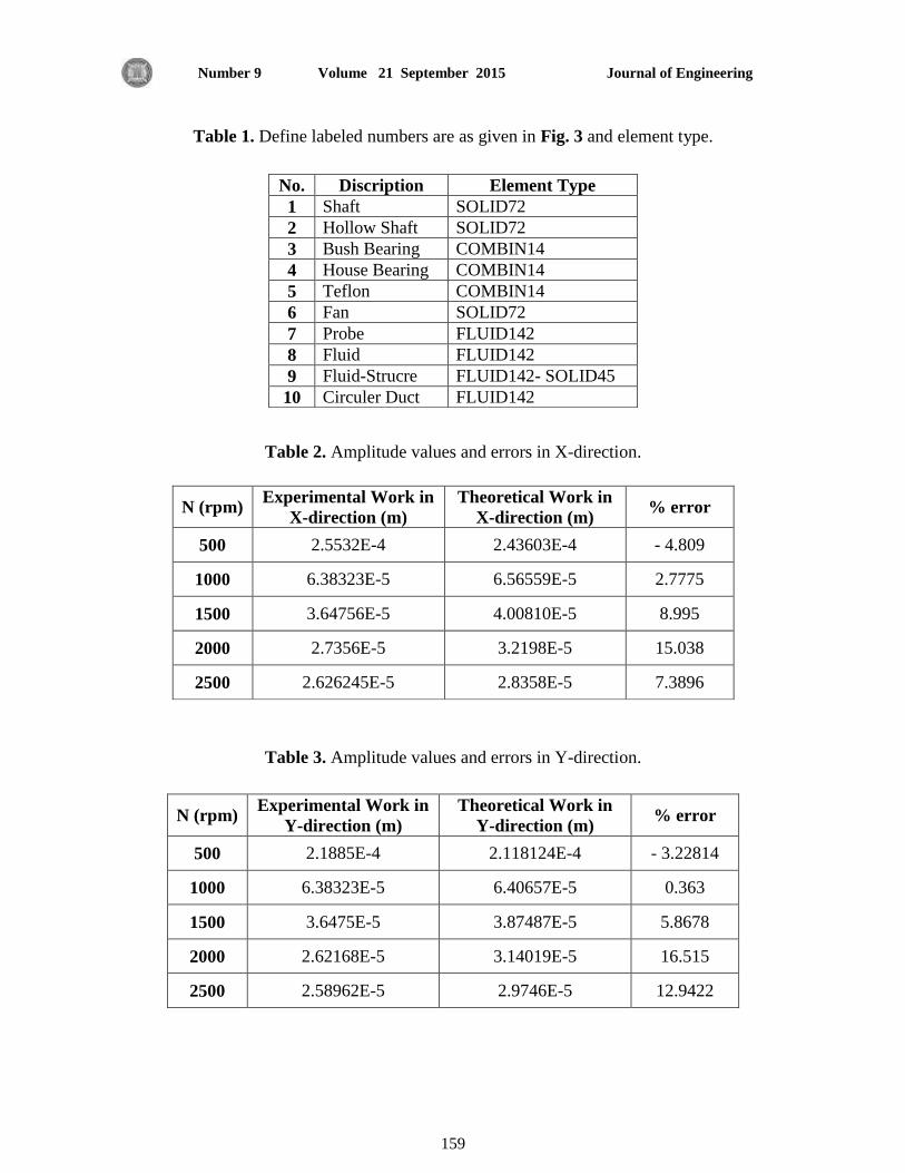
Journal of Engineering Volume 21 September 2015 Number 9
159
Table 1. Define labeled numbers are as given in Fig. 3 and element type.
Table 2. Amplitude values and errors in X-direction.
N (rpm) Experimental Work in
X-direction (m)
Theoretical Work in
X-direction (m) % error
500 2.5532E-4 2.43603E-4 - 4.809
1000 6.38323E-5 6.56559E-5 2.7775
1500 3.64756E-5 4.00810E-5 8.995
2000 2.7356E-5 3.2198E-5 15.038
2500 2.626245E-5 2.8358E-5 7.3896
Table 3. Amplitude values and errors in Y-direction.
N (rpm) Experimental Work in
Y-direction (m)
Theoretical Work in
Y-direction (m) % error
500 2.1885E-4 2.118124E-4 - 3.22814
1000 6.38323E-5 6.40657E-5 0.363
1500 3.6475E-5 3.87487E-5 5.8678
2000 2.62168E-5 3.14019E-5 16.515
2500 2.58962E-5 2.9746E-5 12.9422
No. Discription Element Type
1 Shaft SOLID72
2 Hollow Shaft SOLID72
3 Bush Bearing COMBIN14
4 House Bearing COMBIN14
5 Teflon COMBIN14
6 Fan SOLID72
7 Probe FLUID142
8 Fluid FLUID142
9 Fluid-Strucre FLUID142- SOLID45
10 Circuler Duct FLUID142
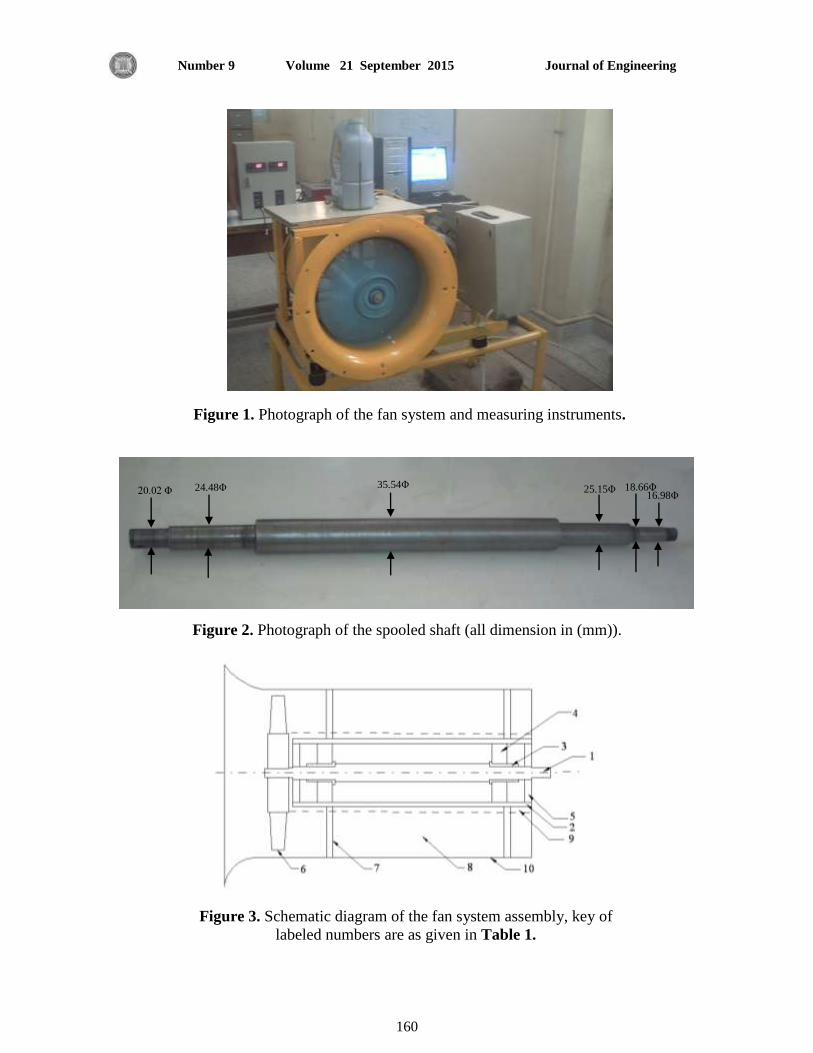
Journal of Engineering Volume 21 September 2015 Number 9
160
Figure 1. Photograph of the fan system and measuring instruments.
Figure 2. Photograph of the spooled shaft (all dimension in (mm)).
20.02 Φ 24.48Φ 35.54Φ 25.15Φ 18.66Φ 16.98Φ
Figure 3. Schematic diagram of the fan system assembly, key of
labeled numbers are as given in Table 1.

Journal of Engineering Volume 21 September 2015 Number 9
161
1st mode shape
2nd mode shape
3rd mode shape 4th mode shape
5th mode shape 6th mode shape
7th mode shape 8th mode shape
9th mode shape 10th mode shape
Figure 4. Natural frequency and mode shape for the spooled shaft.
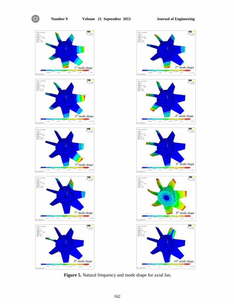
Journal of Engineering Volume 21 September 2015 Number 9
162
1st mode shape
2nd mode shape
3rd mode shape 4th mode shape
5th mode shape 6th mode shape
7th mode shape 8th mode shape
9th mode shape 10th mode shape
Figure 5. Natural frequency and mode shape for axial fan.
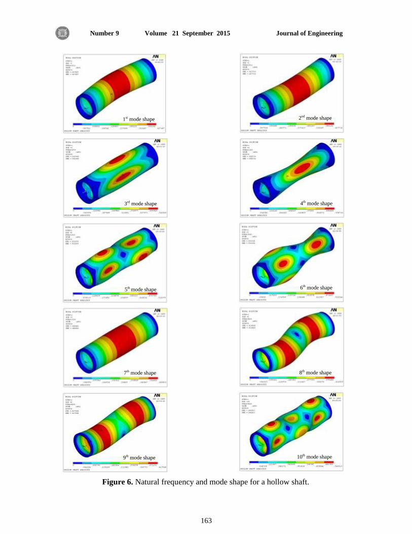
Journal of Engineering Volume 21 September 2015 Number 9
163
Figure 6. Natural frequency and mode shape for a hollow shaft.
1st mode shape
2nd mode shape
3rd mode shape 4th mode shape
5th mode shape 6th mode shape
7th mode shape 8th mode shape
9th mode shape 10th mode shape
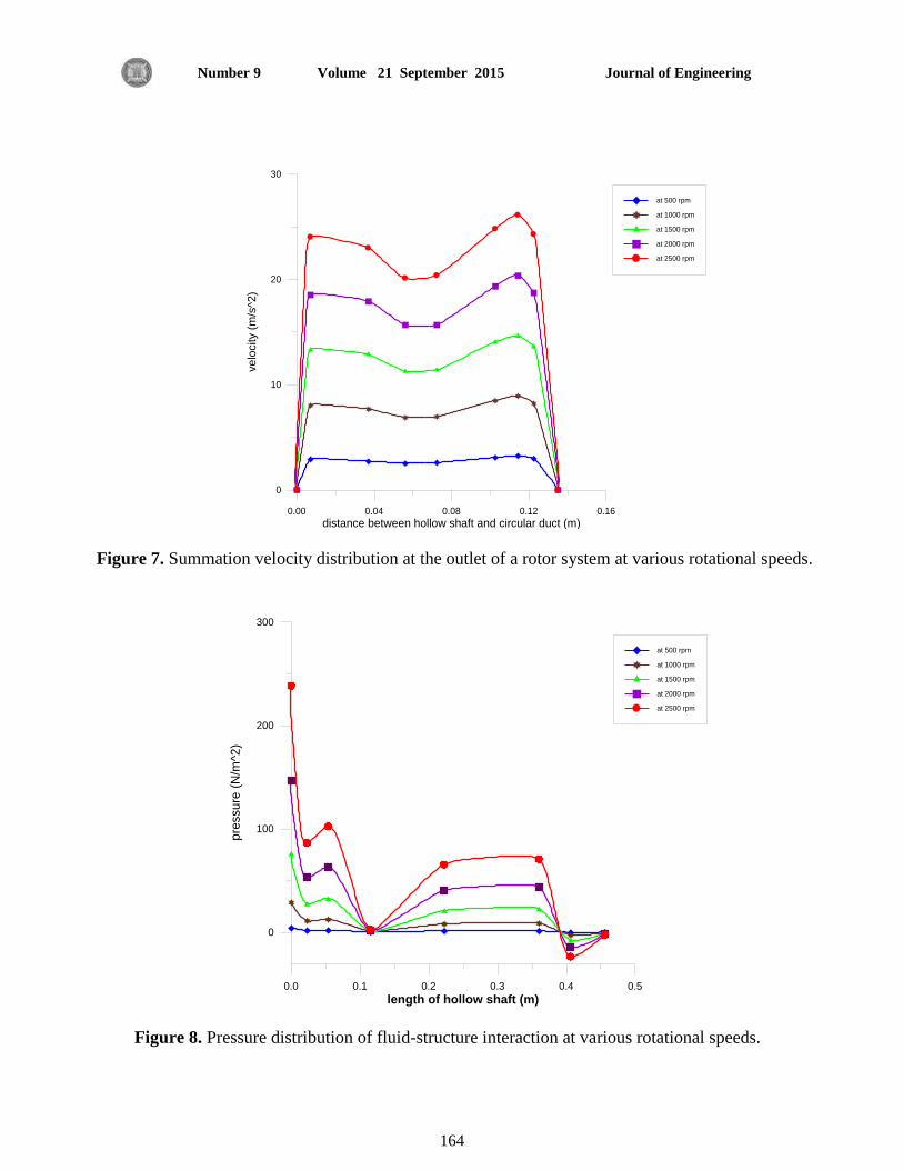
Journal of Engineering Volume 21 September 2015 Number 9
164
0.00 0.04 0.08 0.12 0.16
distance between hollow shaft and circular duct (m)
0
10
20
30
velo
city (
m/s
^2
)
at 500 rpm
at 1000 rpm
at 1500 rpm
at 2000 rpm
at 2500 rpm
0.00 0.04 0.08 0.12 0.16
distance between hollow shaft and circular duct (m)
0
10
20
30
velo
city (
m/s
^2
)
at 500 rpm
at 1000 rpm
at 1500 rpm
at 2000 rpm
at 2500 rpm
Figure 7. Summation velocity distribution at the outlet of a rotor system at various rotational speeds.
0.0 0.1 0.2 0.3 0.4 0.5
length of hollow shaft (m)
0
100
200
300
pre
ssu
re (
N/m
^2)
at 500 rpm
at 1000 rpm
at 1500 rpm
at 2000 rpm
at 2500 rpm
0.00 0.04 0.08 0.12 0.16
distance between hollow shaft and circular duct (m)
0
10
20
30
velo
city (
m/s
^2
)
at 500 rpm
at 1000 rpm
at 1500 rpm
at 2000 rpm
at 2500 rpm
Figure 8. Pressure distribution of fluid-structure interaction at various rotational speeds.

Journal of Engineering Volume 21 September 2015 Number 9
165
Figure 11. Static stress analysis of system parts and system at rotational speed (1500) rpm.
Figure 9. Static stress analysis of system parts and system at rotational speed (500) rpm.
Figure 10. Static stress analysis of system parts and system at rotational speed (1000) rpm.

Journal of Engineering Volume 21 September 2015 Number 9
166
Figure 12. Static stress analysis of system parts and system at rotational speed (2000) rpm.
Figure 13. Static stress analysis of system parts and system at rotational speed (2500) rpm.
Figure 14. Non-synchronous vibration amplitude for a rotor system in X and Y-directions at (500) rpm.
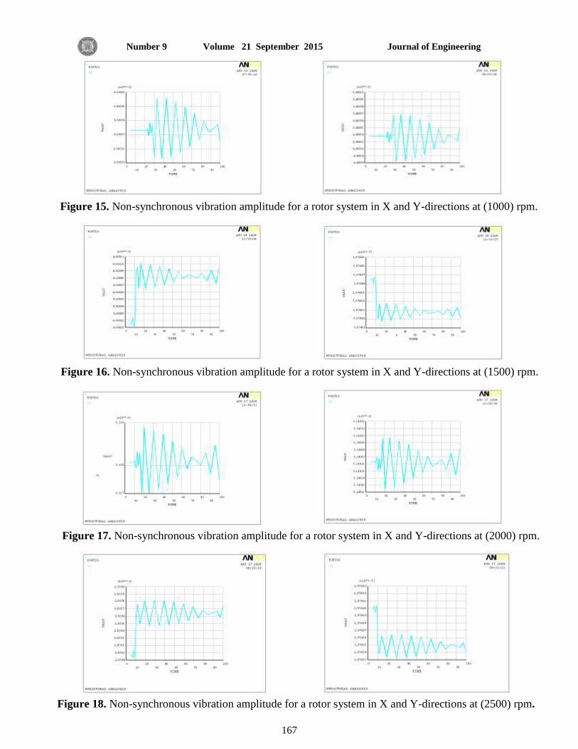
Journal of Engineering Volume 21 September 2015 Number 9
167
Figure 15. Non-synchronous vibration amplitude for a rotor system in X and Y-directions at (1000) rpm.
Figure 16. Non-synchronous vibration amplitude for a rotor system in X and Y-directions at (1500) rpm.
Figure 17. Non-synchronous vibration amplitude for a rotor system in X and Y-directions at (2000) rpm.
Figure 18. Non-synchronous vibration amplitude for a rotor system in X and Y-directions at (2500) rpm.

Journal of Engineering Volume 21 September 2015 Number 9
168
0 500 1000 1500 2000 2500 3000
N (rpm)
0
1E-4
2E-4
3E-4
Ux (
m)
experimental work
theoretical work
Figure 19. Experimental and theoretical amplitude in X-direction.
0 500 1000 1500 2000 2500 3000
N (rpm)
0.0E+0
5.0E-5
1.0E-4
1.5E-4
2.0E-4
2.5E-4
Uy (
m)
experimental work
theoretical work
Figure 20. Experimental and theoretical amplitude in Y-direction.

Journal of Engineering Volume 21 September 2015 Number 9
1
Experimental Study on the Effect of Using Metallic Brushes on the Charging
and Discharging Time of Thermal Energy Storage Unit
Asst. Prof. Dr. Rafa Abbas Hassan
Mechanical Engineering Department
College of Engineering
University of Al Mustansiriyah
Email:[email protected]
Lecturer. Dr. Aseel Khaleel Shyaa
Mechanical Engineering Department
College of Engineering
University of Al Mustansiriyah
Email:[email protected]
Ban Mohammed Hasan Kadim
Mechanical Engineering Department
College of Engineering
University of Al Mustansiriyah
Email:[email protected]
ABSTRACT
Phase change materials are known to be good in use in latent heat thermal energy storage
(LHTES) systems, but one of their drawbacks is the slow melting and solidification processes.
So that, in this work, enhancing heat transfer of phase change material is studied experimentally
for in charging and discharging processes by the addition of high thermal conductive material
such as copper in the form of brushes, which were added in both PCM and air sides. The
additions of brushes have been carried out with different void fractions (97%, 94% and 90%) and
the effect of four different air velocities was tested. The results indicate that the minimum brush
void fraction gave the maximum heat transfer in PCM and reduced the time for melting for
(ϵ=90%) up to 4.49 times as compare with the case of no brush. It can be seen that the addition
of brushes in air side helped to reduce the solidification time and increase the convection heat
transfer coefficient as the brush void fraction decreased. Also the minimum velocity (v = 1 m/s)
gave maximum outlet temperature.
Keywords: Thermal storage, Phase change materials, Latent heat thermal energy storage and
heat transfer enhancement.
دراست عوليت على تأثير استخذام فرش هعذيت على الوادة الوتغيرة الطور الخازت للطاقت
حسي عباس رافع أ.م.د.
قسن الهذست الويكايكيت
كليت الهذست/الداهعت الوسخصشيت
شياع خليل اسيل م.د.
قسن الهذست الويكايكيت
الوسخصشيت الداهعت/الهذست كليت
كاظن حسي هحوذ باى
قسن الهذست الويكايكيت
تالوسخصشي الداهعت/الهذست كليت
الخلاصت
في هظوهاث خضى الطاقت الحشاسيةت الكاهةتو كلكةي اعةذ هيو هةا الوسخخذهت الوواد الوخغيشة الطوس حعذ هي الوواد الديذة
ححسةيي اخاةاا الحةشاسة للوةواد الوخغيةشة الطةوس خةةا هوليةت ال ةحي في العول الحةالي حةن دساسةتهو الاصهاسكالادواد بطء.
كرلك أضافت هادة لها هوصليت عشاسيت هاليت هثل الحاط كالزي سوف يكوى كل فششو كهةز الفةشش سةوف هوليا كالخفشيغ
%( هة اخخبةاس 70 % ك79%و 79حضاف في خاب الوادة الوخغيشة الطةوس كخاةب الهةواء. حوةج اضةافت الفةشش سةب فةشا
حأثيش اس سةش هخخلفةت. كقةذ يةج الخةا ح اى اقةل سةبت فةشا للفش ةاة اهطةد اكبةش صيةادة فةي سةبت اخاةاا الحةشاسة فةي الوةادة
هشة الوااست ه عالت هذم كخود الفش اة. كقةذ 79.9( الد ϵ% = 70الوخغيشة الطوس حيث قل الضهي الةصم لةصهاس لحالت
ةصم لةدوةاد ككةزلك صادث هةي هعاهةل اخاةاا الحةشاسة لةى اضافت الفشش في خضء الهواء ساهذ في حاليةل الةضهي الوعظ ايضا ا
واسطت الحول اصاى السبت الفشاغيت للفش اة. ككزلك كخذ اى اقل سشهت هسخخذهت اهطج اكبش عشاسة للهواء الخاسج.
.الطوسو خضى الطاقت الحشاسيت الكاهت ك ححسيي اخااا الحشاسةالخضى الحشاسيو هواد هخغيشة الكلواث الرئيسيت:

Journal of Engineering Volume 21 September 2015 Number 9
2
1. INTRODUCTION
Solar energy is one of the most important types of renewable energy because it is one of
the cleanest energy and has no impurities into the environment, also it is infinite. Thermal energy
storage systems (TESS) are one type of renewable energy systems in which they were developed
to use the solar energy in night or in case of dust or clouds. TESS is of critical importance in
many engineering applications. The demand for CO2 reduction to curb global warming
considerably increases the interest in utilizing renewable energy sources, especially solar energy
Zhao, et al., 2010. TESS is one of the most important applications of phase change materials
(PCMs). They can be applied conveniently in many fields such as peak shift of electrical
demands, solar energy utilization, waste heat recovery, intelligent air-conditioned buildings, and
temperature controlled greenhouses, electrical appliances with thermostatic regulators, energy
storage kitchen utensils, insulation clothing and season storage Molefi, 2008. They can be
classified into three main categories according to different storage mechanisms: sensible heat
storage, latent heat storage and chemical heat storage. To date most of the studies conducted on
storage materials have concentrated on sensible and latent heat storage systems. Studies
conducted to compare phase change and sensible heat storages have shown that a significant
reduction in storage volume can be achieved using PCM compared to sensible heat storage Tian,
2012. There are mainly three types of PCMs existing in the solid-liquid category: organic-PCM,
inorganic-PCM and eutectic-PCM. In order to be utilized for real applications, PCMs need to
meet the thermal, physical, kinetic, chemical and economical requirements Sunliang, 2010.
Materials to be used for phase change thermal energy storage must have high latent heat of
fusion and high thermal conductivity. They should also have a melting temperature lying in a
practical range of operation, melt uniformly, chemically inert, low cost, non toxic and non
corrosive. As paraffin wax possesses most of these properties it attracts considerable attention as
a PCM. However, paraffin waxes have inherently low thermal conductivity and so it takes
considerable time to melt and solidify, which reduces the overall power of the thermal storage
device and thereby restrict their application Vadwala, 2011.
Most PCMs have low thermal conductivity, which led to slow melting and solidification.
Different studies have been done to enhance heat transfer in PCMs which include, for example,
the addition of water bubbles Velraj, et al., 1999, carbon fiber brushes Fukai, et al., 2002,
longitudinal fins Castell, et al. , 2006, metallic powder Bellah, and Ghazy, 2007, graphite Zhang,
et al., 2011, metal foam Vadwala, 2011, nanofibers Sanusi, et al., 2011and metallic particles
Hasan, 2013.
Velraj, et al., 1999, investigated three methods of enhancing the heat transfer rate of
paraffin wax encapsulated in a cylindrical aluminum tube using internal longitudinal aluminum
fins, steel Lessing rings and water bubbles. It found that the best enhancement method was by
using of Lessing rings (20% by volume) in which they decrease the freezing time by a factor of
9, and increase thermal conductivity about 10 times than pure paraffin. Also the finned tube with
a volume fraction of 7% decrease the solidification time to about 4 times of that of no fins.
Fukai, et al., 2002, improved the heat transfer rate during the charge and discharge processes by
making use carbon fiber brushes combined with n-octadecane. Carbon fiber improves the
thermal conductivities of phase-change materials packed around heat transfer tubes. The thermal
conductivity increased as the volume fraction and diameter of fibers increased. It was found that
the use of brushes improved the charging and discharging rate to about 20% and 30%,
respectively, higher than that using no fibers. Castell, et al., 2006, study the effect of using
longitudinal vertical fins inside a cylindrical water tank which contain cylindrical PCM modules.
The experiments were done with three different cases, without fins, with fins of 20mm height
Journal of Engineering Volume 21 September 2015 Number 9
3
and with fins of 40 mm height. It was found that the use of these fins should increase the heat
transfer coefficient up to 3 times larger than the ones without fins. Also, they reduced the time
which was required for solidification of PCM to about 23.53% and 58.82% for the cases of 20
mm and 40 mm height respectively. Bellah, and Ghazy, 2007, made use of 80 μm aluminum
powder with PCM in a solar collector. It was found that the addition of 0.5 mass fraction of
powder decrease the charging time up to 60% as compare with the case of pure paraffin. Zhang,
et al., 2011, tried to improve the thermal conductivity of paraffin by using expanded graphite
with 7% mass fraction. The results show that the graphite/paraffin composite PCM made 44%
reduction in heat storage duration and 69% reduction in the retrieval duration, respectively, as
compared with the pure paraffin. Vadwala, 2011, placed copper foam (85% porosity) in a
rectangular TESS for both PCM (paraffin wax) and air sides. The results show that the thermal
conductivity of PCM was increased to about 18 times that of pure paraffin. The time required to
melt the same quantity of wax was reduced to 36% of that without foam. Also it was found that
the addition of metal foam in the air side decreases solidification time. Sanusi, et al., 2011, study
experimentally the effect of graphite nanofibers on thermal storage and the solidification time
with different aspect ratios. It was found that the addition of these fibers reduce the maximum
temperature in the thermal containment unit up to 48%. Also the results showed a reduction in
the solidification time up to 61% for the case of 1 aspect ratio. Hasan, 2013, made a Comparison
between Different Composite PCMs encapsulated for TESS. The thermal conductivity of
paraffin had been enhanced by using four different additives which were graphite powder,
copper particles, aluminum oxide particles and copper network. The mass ratios of the additives
were 3%, 6% and 9%. It was found that copper network with 6% mass ratio gave best
enhancement which reduce the time for charging and discharging by 26.4% and 30.3%
respectively as compared with pure paraffin. Also thermal conductivity of PCM enhanced
by2.57 times than pure paraffin.
The objective of this work is to study experimentally the enhancement of charging and
discharging processes by using copper brushes embedded in both PCM and air sides with
different void fractions. The effect of air velocity was also observed.
2. EXPERIMENTAL TEST
2.1 Experimental Setup
A small scale thermal energy storage device is fabricated, both with and without copper
brush. A paraffin wax grade B (melting temperature equal to 63.7˚C, k= o.214 W/m.˚C) was
employed as heat storage media. The experimental setup is shown schematically in Fig. 1. It
consists of entry section, test section, exit section and transition section. The length of each
section is about 1070 mm, 300 mm, 390 mm and 380 mm, respectively. A transition section
connects between the entry section and a fan with specification of (0.27 A, 61 W, 3100 rpm).
The dimension of the test section was 300 mm × 90 mm × 86 mm (L × W × H). The height of
the air side and PCM side were 42 mm and 32 mm, respectively. A Perspex sheet with 9 mm
thickness was used to form the test section. A copper plate (2.5 mm thick) is used to separate
each side & was placed in two slots (3 mm thick) opposing each other. Other opposing slots of
the same thickness of the former ones were in the upper part of the PCM side and another copper
plate was placed inside it. In the upper side of this plate, a tape heater (150 W, 260 V) with
dimensions of 280 mm× 65 mm, was fixed over it. To ensure good contact between the heater
and the copper plate, a heat-conductive paste was used. For each copper plate, a thermocouple
type K had been fixed in the middle of them. Other five thermocouples type K were distributed
approximately in the center of PCM side with 10 mm distance between adjacent thermocouple.
The top thermocouple should be connected to the process controller which works to control the

Journal of Engineering Volume 21 September 2015 Number 9
4
heater to give a constant temperature of 100◦c for the upper plate, so that it should be an input to
it.
Six thermocouples type K had been distributed in the air passage, one in the entrance, one
in the exit and the others are distributed along the centre plane of the air side with equal spaces
between them (70 mm spaces). A data logger device (model: BTM-4208SD, Lutron electronic
enterprise company) is used to record the data. Fiberglass insulation (12.7 mm thick) with an
aluminized outer surface had been used to insulate the test section. The air velocity of 1, 2, 2.5
and 3 m/s is produced by a fan which was controlled by a fan controller by changing the voltages
entering to it. These velocities had been measured by a hot wire anemometer (model: YK-
2005AH, Lutron electronic enterprise company) fixed in the entrance of the test section.
Two copper brushes had been placed in PCM side which had a diameter equal to the height
of the PCM container. So that, each wall was in contact with brushes copper wires. Other two
brushes were placed in the air side, and also they had a diameter equal to the air side height. The
length of all brushes is equal to the test section length. In each side the tests should be done with
three different void fraction 97%, 94% and 90%. The void fraction of each brush had been
calculated using standard test method (ASTM C 127). The brushes are weighted with gram unit
in air and then in water to get there densities in air and water and then calculate void fraction (ϵ)
using Eq. (3). The following equations are using for that purpose:
ρa =
ρw =
ϵ =
Where;
ma = mass of weighted material in air, (g).
mw = mass of weighted material in water, (g).
Vb = bulk volume of used material, (cm3).
ρb = bulk material density, (g/cm3).
ρw = density of material in water, (g/cm3).
ϵ = void fraction, (%).
Because of the high thermal conductivity of the copper wires (k= 385 W/m.˚C), the PCM
brushes work to enhance thermal conductivity and reduce the time for paraffin wax melting.
Also the addition of brushes in air side work to decrease the time of solidification.
2.2 Experimental Procedure
Several experimental tests were done with different cases. First of all, the molten paraffin
wax was poured into the test rig. After its solidification, a gap of air would be appear in the
upper part of the test section because of the decrease in volume of PCM due to differences in
solid and liquid densities. After the fixation of the whole TESS, the melting and solidification
tests (without brush) should be done for different velocities. A process controller was setup to
control the heater to provide constant temperature (100˚C) to the top copper plate. The melting
time starts from the time the heater turned on, till the lower copper plate reaches a temperature of
63.7◦c. after the heater turned off, the fan turned on and the solidification process starts. The fan

Journal of Engineering Volume 21 September 2015 Number 9
5
was controlled via a fan controller to get the required velocities. This process ended until the
whole wax reached its starts temperature. So that, as the charging time is over, the discharging
time begins.
The previous processes should be repeated but with the addition of copper brushes in both
air and wax sides. Also, the tests should be done with different void fractions (97%, 94% and
90%) to show the effect of the void fraction in charging and discharging processes. Fig.2 shows
these brushes and their position.
3. EXPERIMENTAL DATA REDUCTION
3.1 PCM Side
3.1.1 Latent heat storage
The heat storage in PCM side is in the form of latent heat. The storage capacity can be
found from:
Q = ∫
. Cps .dT + m . am . ∆ hm + ∫
. Cpl . Dt
= m [ Cps (Tm – T1) + am . . ∆ hm + Cpl (T2 – Tm)] (1)
Where;
Tm = melting temperature of the storage material, ˚C.
T1 = initial temperature of the storage material, ˚C.
T2 = final temperature of the storage material, ˚C.
m = mass, kg.
Cpl = average specific heat between Tm and T2, J/kg.˚C.
Cps = average specific heat between T1 and Tm, J/kg.˚C.
am = the fraction melted.
∆ hm = heat of fusion, J/kg.
It can be seen that the second term represents the period in which phase change occurs
during it, which means that it is the period for transformation from solid to liquid and vice versa.
Conduction heat transfer: The heat transfer inside the PCM occurs due to conduction between its
particles. The conduction occurs from the upper surface of PCM to the lower surface of PCM.
The following equation represents Fourier's law for heat conduction:
Q = k A ΔT/Δx (2)
Where;
Q = power extracted, W.
A = area, m2.
∆T = temperature difference between the upper and lower point of PCM, ˚C.
∆x = distance between the upper and the lower point of PCM, m.

Journal of Engineering Volume 21 September 2015 Number 9
6
3.2 Air Side
The following procedure was used to calculate mass flow rate, Nusselt number, Reynold
number, convection heat transfer coefficient and power extracted. The experimental data
includes the measured velocities and thermocouples readings. The air thermo physical properties
were taken at bulk mean air temperature;
Tb =
(3)
Where;
Tb = bulk temperature of air, ˚C.
Ti = inlet air temperature, ˚C.
To = outlet air temperature, ˚C.
3.2.1 Mass flow rate
Mass flow rate can be calculated using the following relation;
m = ρ v Ac (4)
Where;
v = velocity, m/s.
Ac = crosses sectional area, m2.
3.2.2 Rate of heat transfer
Value of heat transfer between the hot surface and the moving air can be calculated
experimentally from;
Q = m Cp (To-Ti) (5)
3.2.3 Convection heat transfer coefficient measurement
Convection occurs between the hot copper plate and the air flow beneath it. It was
considered to be constant along the duct length. So that it is given by;
h =
(6)
Where;
Ts = surface temperature, ˚C.
As = surface area, m2.
3.2.4 Reynolds number
It is calculated from;
Re =
(7)
Where;

Journal of Engineering Volume 21 September 2015 Number 9
7
Re = Reynolds number.
μ = dynamic viscosity, kg/m.s.
In which DH is the hydraulic diameter and can be calculated from;
DH =
(8)
Where;
W = width, mm.
H = height, mm.
3.2.5 Nusselt number
It can be calculated using the following equation;
Nu =
(9)
4. RESULTS AND DISCUSSION
This work investigates the effect of copper brush on the melting and solidification time of
an organic PCM (paraffin wax grade B). Fig. 3 shows the lower copper plate temperature
variation with time for four cases, without brush, with brush (ϵ=97%), with brush (ϵ=94%) and
with brush (ϵ=90%). The time for melting was decreased up to 2.67, 3.71, 4.49 times,
respectively, as compare with the pure paraffin case, which means that the heat transfer was
enhanced.
Fig. 4 shows the behavior of middle point temperature of PCM in melting and
solidification process. It can be seen that the melting and solidification time was decrease in the
addition of metal brush as compared with pure paraffin, where the lower void fraction, the lower
time for melting and solidification. The copper brushes reduced the solidification time of paraffin
up to 1.47, 1.55 and 1.64 when they add in both sides with 3%, 6% and 10% volume percent,
respectively, as compared with pure paraffin case.
It can be seen from Fig. 5 the temperature distribution of five points distributed along PCM
in case of brushes with 90% void fraction during melting process. The middle point was melted
faster than other points because it was the furthest point from the walls. Also the lower point
takes longer time to melt due to its distance to the upper copper plate.
Fig. 6 presents that the lower void fraction of brush in air side gave the maximum outlet
temperature. This was due to the increase in contact between the upper copper plate and the
brush wires which cause an increase in heat transfer from copper plate and brush to the air flow
over them. So that, the decrease in void fraction cause an increase in turbulent which helps to
increase the heat exchange between them. The amount of increase in outlet temperature for (ϵ=
97%, 94% and 90%) as compared with the case of no brush were 8.75, 10.32 and 11.99 ˚C,
respectively with 2.5 m/s air velocity, in which these values are taken as hourly temperature.
The outlet air temperature vs. time was shown in Fig. 7 during solidification process with
four different velocities in case of brushes (ϵ=90%) in both wax and air side. As compared with
the case of no brushes in both sides, it can be seen that the maximum temperature difference
reach up to (21.85˚C) occurred in case of minimum void fraction (90%) and minimum velocity
(v=1 m/s). That is because at low velocity (v=1 m/s) air will has enough time to acquire heat and
Journal of Engineering Volume 21 September 2015 Number 9
8
make heat exchange with the lower copper plate. While at maximum velocity (v=3 m/s) air will
be pass beneath the lower plat quickly.
Also, the higher the velocity, the minimum the outlet temperature and the maximum the
temperature gradient. The results show that the decrease in void fraction of brushes in air side
cause an increase in Nusselt numbers due to a significant increase in outlet air temperature which
resulted in higher Nusselt number for the three void fractions (97%, 94%90%). This increase, as
shown in Fig. 8, was up to 2.83, 3.69 and 4.23 times, respectively, as compared with the case of
no brush. Fig. 9, 10, shows the relation between velocities with power extracted and convection
heat transfer coefficient with different brushes void fractions. As in Nusselt numbers, for lower
void fraction, higher power and convection heat transfer coefficient are obtained. The amounts of
increase in power for (ϵ=97%, 94%, 90%) were 2.24, 2.49 and 2.83 times, respectively, and 2.9,
3.79 and 4.34 times, respectively, for h as compared with the case of no brush. The results in
Figs. 8, 9 and 10 were taken as an average values for hourly temperature.
5. CONCLUSION In this work, the thermal conductivity of wax and heat transfer coefficient of flowing air
was enhanced by using copper brushes. The enhancement process done to reduce the time for
melting and solidification by the addition of brushes in wax and air sides, the following
conclusions can be extracted:
The addition of brushes in PCM side reduce the time for melting for (ϵ=90%) by 4.46
times as compare with the case of no brushes. It can be seen that, for lower void fraction,
minimum melting time is obtained. The addition of brushes in air side worked to enhance the
discharging process, and also reduce the time required for solidification. Lowest void fraction in
air side decreases the solidification time and increases the outlet air temperature. The maximum
temperature difference reached up to 21.85˚C which occurred in case of minimum void fraction
and minimum velocity. The obtained results show that minimum velocity gave maximum outlet
temperature. But maximum velocities increased the heat transfer rate especially in the initial
period which resulted in minimum time required for freezing. Also, at minimum void fraction
and maximum velocity, higher Nu, h and Q for air can be observed. This is because of increase
in turbulence which causes an increment in heat transfer rate.
REFERENCES
Bellah, E., and Ghazy, A., 2007, Thermal Conductivity Enhancement in Latent Heat
Storage System, Solar Energy, Vol. 81, 839–845.
Castell, A., Solé, C., Medrano, M., Roca, J., García, D.,and Cabeza, L., F., 2006, Effect of
Using External Vertical Fins in Phase Change Material Modules for Domestic Hot
Water Tanks.
Fukai, J., Hamada, Y., Morozumi, Y., and Miyatake, O., 2002 , Effect of Carbon Fiber
Brushes on Conductive Heat Transfer in Phase Change Materials, International Journal
of Heat and Mass Transfer, Vol. 45, 4781-4792.
Hasan, A. H., 2013, Comparison Between Different Composite Phase Change Materials
for Latent Heat Encapsulated Thermal Energy Storage, M.Sc Thesis, University of Al
Mustansiriyah.

Journal of Engineering Volume 21 September 2015 Number 9
9
Molefi, J. A., 2008, Investigation of Phase Change Conducting Materials Prepared from
Polyethylenes, Paraffin Waxes and Copper, PhD thesis, university of the free state.
Sanusi, O., Warzoha, R., and Fleischer, A. S., 2011, Energy Storage and Solidification of
Paraffin Phase Change Material Embedded with Graphite Nanofibers, International
Journal of Heat and Mass Transfer, 54 4429–4436.
Sunliang, C., 2010, State of the Art Thermal Energy Storage Solutions for High
Performance Buildings, M.Sc Thesis, University of Jyväskylä, Finland.
Tian, Y., 2012, Heat Transfer Enhancement in Phase Change Materials (PCMs) by
Metal Foams and Cascaded Thermal Energy Storage, PhD Thesis, University of
Warwick.
Vadwala, P. H., 2011, Thermal Energy Storage in Copper Foams Filled with Paraffin
Wax, Msc Thesis, University of Toronto.
Velraj, R., Seeniraj, R. V., Hafner, B., Faber, C., and Schwarzer, K., 1999, Heat Transfer
Enhancement in a Latent Heat Storage System, Solar Energy, 65(3), pp. 171- 180.
Zhang, P., Xia, L., and Wang, R. Z., 2011, the Thermal Response of Heat Storage System
with Paraffin and Paraffin/Expanded Graphite Composite for Hot Water Supply, World
Renewable Energy Congress.
Zhao, C. Y., Lu, W., and Tian, Y., 2010, Heat Transfer Enhancement for Thermal
Energy Storage Using Metal Foams Embedded within Phase Change Materials (PCMs),
Solar Energy , 84(8), pp. 1402-1412.
NOMENCLATURE am = the fraction melted.
Ac = crosses sectional area, m2.
As = surface area, m2.
Cp = specific heat of air, J/kg.˚C.
Cpl = average specific heat between Tm and T2, J/kg.˚C.
Cps = average specific heat between T1 and Tm, J/kg.˚C.
DH = hydraulic diameter, m.
h = convection heat transfer coefficient, W/m2.˚C.
∆ hm = heat of fusion, J/kg.
H = height, mm.
K = thermal conductivity, W/m.˚C.
L = length, mm.
m = mass, kg.
ma = mass of weighted material in air, (g).
mw = mass of weighted material in water, (g).
Nu = Nusselt number, dimensionless.
Q = power extracted, W.
Re = Reynolds number.

Journal of Engineering Volume 21 September 2015 Number 9
11
t = time, minute.
T = temperature, ˚C.
∆T = temperature difference between the upper and lower point of PCM, ˚C .
Tb = bulk temperature of air, ˚C.
TC = thermocouple.
Ti = inlet air temperature, ˚C.
Tm = melting temperature of the storage material, ˚C.
Tmid = middle temperature of the storage material, ˚C.
To = outlet air temperature, ˚C.
Ts = surface temperature, ˚C.
T1 = initial temperature of the storage material, ˚C.
T2 = final temperature of the storage material, ˚C.
v = velocity, m/s.
Vb = bulk volume of used material, (cm3).
W = width, mm.
∆x = distance between the upper and the lower point of PCM, m.
Greek symbols.
ϵ = void fraction, %.
μ = dynamic viscosity, kg/m.s.
ρ = density, kg/m3.
ρb = bulk material density, (g/cm3).
ρw = density of material in water, (g/cm3).
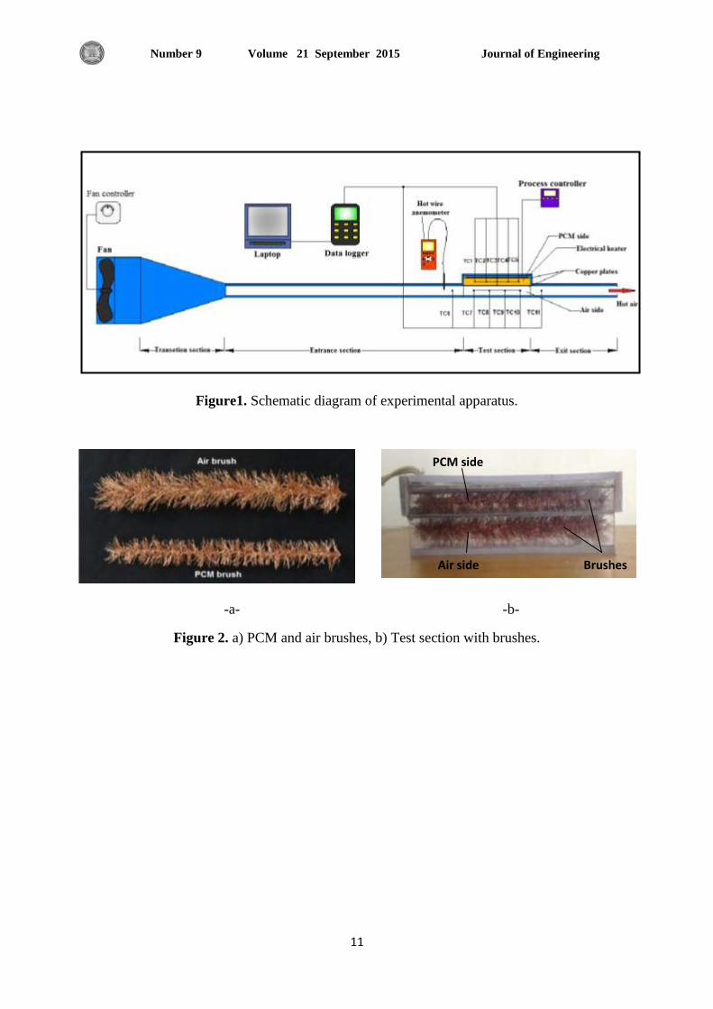
Journal of Engineering Volume 21 September 2015 Number 9
11
Figure1. Schematic diagram of experimental apparatus.
-a- -b-
Figure 2. a) PCM and air brushes, b) Test section with brushes.
Air side
PCM side
Brushes

Journal of Engineering Volume 21 September 2015 Number 9
12
Figure3. Temperature variation of bottom point of paraffin wax vs. time during melting process
for the cases of brushes with different void fractions.
Figure 4. Temperature variation and the melting and solidification point of middle PCM point in
charging and discharging processes with and without brushes for different void fractions. The
discharging process is conducted for velocity of 2.5 m/s.

Journal of Engineering Volume 21 September 2015 Number 9
13
Figure 5. Temperature distribution for different points along the axial center line of PCM during
melting process in case of brushes with 90% void fraction.
Figure 6. The change in outlet air temperature vs. time in cases of brushes in both wax and air
side with three void fractions brushes compared with the case of no brush for an air velocity of
2.5 m/s for an hour.
0
10
20
30
40
50
60
70
80
0 10 20 30 40 50 60 70 80 90
Tem
pe
ratu
re, T
(°C
)
Time, t (min)
TC1
TC2
TC3
TC4
TC5
TC6

Journal of Engineering Volume 21 September 2015 Number 9
14
Figure 7. Change with time in outlet air temperature with brushes in both sides for different
velocities compared with the case of no brushes for an air velocity of v=2.5 m/s for an hour.
Figure 8. The computed Nusselt numbers with respect to Reynolds number for the cases of
different void fractions brushes on both sides compared with the case of no brushes.
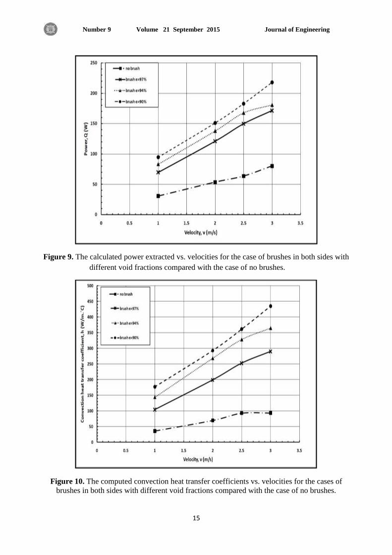
Journal of Engineering Volume 21 September 2015 Number 9
15
Figure 9. The calculated power extracted vs. velocities for the case of brushes in both sides with
different void fractions compared with the case of no brushes.
Figure 10. The computed convection heat transfer coefficients vs. velocities for the cases of
brushes in both sides with different void fractions compared with the case of no brushes.

Journal of Engineering Volume 21 September 2015 Number 9
535
Application of Box-Behnken Method Based ANN-GA to Prediction of wt.%
of Doping Elements for Incoloy 800H Coated by Aluminizing-Chromizing
Dr.Abbas Khammas Hussein
Assistant Professor
University of Technology ,Department of Materials Engineering
Email: [email protected]
ABSTRACT
In this work , an effective procedure of Box-Behnken based-ANN (Artificial Neural Network) and GA
(Genetic Algorithm) has been utilized for finding the optimum conditions of wt.% of doping elements
(Ce,Y, and Ge) doped-aluminizing-chromizing of Incoloy 800H . ANN and Box-Behnken design method
have been implanted for minimizing hot corrosion rate kp (10-12
g2.cm
-4.s
-1) in Incoloy 800H at 900
oC .
ANN was used for estimating the predicted values of hot corrosion rate kp (10-12
g2.cm
-4.s
-1) . The optimal
wt.% of doping elements combination to obtain minimum hot corrosion rate was calculated using genetic
algorithm approach . The predicted optimal values for minimizing hot corrosion rate for Incoloy 800H
coated by (Ce-Y-Ge) doped-aluminizing-chromizing are (3wt.%Ce, 3wt.%Y, and 3wt.%Ge) , the hot
corrosion rate kp (10-12
g2.cm
-4.s
-1) value at these conditions was found to be 71.701 . The results have been
verified by confirmation experiment , results obtained by GA method match closely with experimental
values (R2=98.30) . EDS and XRD results show that the formation of protective layers Al2O3 and Cr2O3
during hot corrosion tests.
Keywords: Box-behnken design, GA, ANN, Hot Corrosion , Pack cementation .
النسب ب للتنبأخوارزميت وراثيت -بينكن ذاث أساس شبكاث عصبونيت إصطناعيت-تطبيق طريقت بوكس
كرمنت-المغطاة بالالمنت Incoloy 800Hالوزنيت المثاليت لعناصر الإضافت لسبيكت
د.عباس خماس حسين
أعرار يغاعذ
انجايعح انركىنىجيح،قغى هذعح انىاد
الخلاصت
خىاسصييح -تيك راخ أعاط شثكاخ عصثىيح إصطاعيح-يرض هزا انثحث إعرخذاو الإعهىب انفعال ي خلال طشيقح تىكظ
كشيح نغثيكح -جشيايىو( نعهيح الأنح-يريشيىو-وساثيح نرحذيذ انظشوف انثهى نهغة انىصيح نعاصش الإضافح )عيشيىو
Incoloy 800H و انشثكاخ انعصثىيح نخفض يعذل انرآكم انغاخ في تيك-رصيى تىكظ. و أعرخذيد كم ي طشيقح ان
900عذ Incoloy 800Hعثيكح oC حيث أعرخذيد انشثكاخ انعصثىيح نهرثؤ تقيى يعذل انرآكم انغاخ ، أيا تانغثح ،
رآكم انغاخ فقذ ذى ذحذيذها تىاعطح نضيج انغة انىصيح انثاني نعاصش الإضافح انلاصيح نهحصىل عهى انقيح انذيا نعذل ان
انغطاج Incoloy 800Hانخىاسصييح انىساثيح . و نىحع أ انقيى انثهى انري ذى انرثؤ تها نخفض يعذل انرآكم انغاخ نغثيكح
أيا (3wt.%Ce, 3wt.%Y, and 3wt.%Ge)كشيح هي -جشيايىو( نعهيح الأنح-يريشيىو-تعاصش الإضافح )عيشيىو
71.701X10يعذل انرآكم انغاخ عذ هز انظشوف فقذ كاد قيح -12
g2.cm
-4.s
-1. و قذ ذى انرحقق ي هز انظشوف ي
خلال ذجشتح انرحقق )انرؤكذ( ، و نىحع أ انرائج انري ذى انحصىل عهيها ي خلال طشيقح انخىاسصييح انىساثيح ذرطاتق تشكم
ذكى طثقاخ انحايح الأوكغيذيح XRDو EDX( . و أظهشخ رائج 98.30دقيق يع انقيى انرجشيثيح )يعايم انرحذيذ=
Al2O3 ،Cr2O3 . خلال إخرثاساخ انرآكم انغاخ
: ذصيى وكظ تيك، انجياخ انىساثيح، انشثكاخ انعصثىيح، انراكم انغاخ ، ذغهيف انغرح .رئيسيتالكلماث ال
Journal of Engineering Volume 21 September 2015 Number 9
536
1.INTRODUCTION
High-temperature oxidation, hot corrosion and erosion are the main failure modes of components
in the hot sections of gas turbines, boilers, etc. Incoloy 800H have been developed for high
temperature applications . This material finds application in the gas turbine industry, constituting
over fifty percent of the gas turbinط weight due to their good mechanical properties at high
temperatures . In general, hot corrosion increases due to the transport in liquid phase of complex
mixtures of molten sodium sulfate which cause catastrophic hot corrosion .,Lin-Chang Tsai1,et.
al., 2015, Fahamsyah H.,et al, 2015, Subhash Kamal, et. al.,2015 . Hot corrosion refers to an
accelerated corrosion, resulting from the presence of salt such as (Na2SO4), NaCl ,V2O5 …ect
that combine to form molten deposits, ط which damage the protective surface oxides . This type
of corrosion occurs when metals are subjected to the temperature range 700–900°C in the
presence of sulphur deposits formed ط as a result of the reaction between sodium chloride and
sulphur compounds in the presence of gas phase surrounding the metals .The Deposits of
(Na2SO4) are molten at higher temperatures (m.p. 884°C) and ط can cause accelerated corrosion
on Ni- and Co-based superalloys. This type of corrosion is commonly called ‘hot corrosion’.,
Subhash Kamal, et al., 2010, T. S. Sidhu,et al.,2006 . Coating techniques play a important role
in the operation at high temperatures, ط particularly for hot section parts, which are subjected to
complex thermal and mechanical strain/stress cycling. Coatings are applied with a specific aim
to improve the base material resistance by provide ط a barrier against high temperatures., Marta
Kianicova ,et al., 2011, W.H Lee and R.Y Lin ,2003 . Pack cementation using aluminum,
chromium or silicon ط is one of the easiest and cheapest processes to obtain the protective
coatings to improve the corrosion resistance at high temperature ., LIN Nai-ming, et al., 2010,
Bruce M., et al., 2001. The diffusion Coating ط method is used for surface alloying of protective
coatings on the substrate surface, for example aluminizing, siliconizing, chromizing,
simultaneousaluminizing-siliconizing,`simultaneous-aluminizing-siliconizing-chromizing and
forms a thin oxide scale, which works as the diffusion barrier and reduces the oxidizing speed of
the base material. , A. ESLAMI, et al., 2009, I.M. Edmonds,et al., 2008, H. R. KARIMI
ZARCHI,et al., 2013 . High temperature oxidation ط resistance is usually improved by the
addition of some amount of oxygen reactive elements (doping elements) like Y and rare earth
elements (REE) Ce, La, Er and others into surface metal. These elements is introduced through
surface treatment techniques such as pack cementation. The incorporation via surface treatment
acts in favour of doping elements concentration at ط the surface where the oxide will form and
thus may have the most benefit, Chao-Chi Jain and Chun-Hao Koo,2007, Ranjan Sinha, et
al.,2013, Hongyu Wang ,et al., 2010.
In this work, ط it has been reported the effects of amounts of oxygen reactive elements (Ce,
Y,Ge) on the parabolic rate constant ط (Hot corrosion rate kp (10-12
g2.cm
-4.s
-1)) through the hot
corrosion experiment of Aluminized-Chromized Superfer 800H (Incoloy 800H) . Recently
many statistical experimental design methods ط have been employed such Box-Behnken design .
These methods involve mathematical models for designing which can be processed using
Artificial Neural ط Network (ANN) and Genetic Algorithm (GA) . The main ط objective of (GA)
is to determine the optimum operational conditions for the coating system .

Journal of Engineering Volume 21 September 2015 Number 9
537
2.MATERIALS AND COATING FORMULATIONS
The experimental work was ط performed by using samples of Superfer800H (Incoloy800) . The
spectrochemical analysis of ط candidate material is shown in Table 1. Samples ط were cut into
squares shapes with dimensions of (10mm× 10×mm×4mm). All ط surfaces , including the edges
were wet ground using 120, 220, 320, 600, 800, and 1200 grit silicon carbide papers. These
samples were ط then cleaned with water, degreased with acetone, and then ultrasonically cleaned
for 30 minutes using ethanol as a medium. After drying, ط the samples were stored in
polyethylene zip-lock bags. The dimensions of all ط samples were measured. The pack ط mixture
used for aluminum-chromium diffusion coating consisting of 20 Wt.%Al powder (m in
particule size) as an ط aluminum source, 10 Wt.%Cr powder (50-m in particule size) as a
chromium source, 2Wt.% NaF and 4Wt.%NaCl as activator and the balance was alumina-
powder (80-110m in particule size). All pack powders were ط sized by sieving method and 1-
3Wt.% of the pack alumina filler was replaced by ط reactive elements (Ce,Y,Ge) according to a
standard response surface ط methodology (RSM) design called Box-Behnken Design (BBD) .
The samples was placed in a sealed stainless steel ط cylindrical retort of 50mm in a diameter and
of 80mm in a height in contact with the pack mixture. The retort was then put in another stainless
steel cylindrical retort of 80mm in a diameter and 140mm in a height. The outer ط retort has a
side tube through which argon gas passes and second in the top cover for argon gas outlet. Type-
k calibrated thermocouple was ط inserted through the cover of the outer retort for recording real
temperature near inner retort. Figure 1 shows ط the apparatus used for pack cementation
(University of Technology / Department of Production Engineering & Metallurgy). Pack
cementation process ط was carried out at 1050 o
C for 6 h under an Ar atmosphere according to
Robert A.Rapp et al procedure, 1991. In order to ط examine the microstructure of the coatings
before and after hot corrosion test at the optimum conditions, the coated and tested samples
were mounted and ground up to 1000 grit with SiC paper and then polished using 1μm diamond
paste. The samples ط were then analyzed using energy dispersive spectroscopy(EDS) , x-ray
diffraction (XRD), and optical microscope .
3.HOT CORROSION TEST
For hot corrosion tests, 75 ط% wt.Na2SO4 and 25%wt. NaCl powders were selected as a
corrosive salts. Samples were ط deposited with each of these salts until a total coating weight of 5
mg/cm2 was reached according to ط A.Anderson et. al procedure,2012 .The samples were
measured and weighed ط first , then placed on a hot plated heated to 110oC. An air gun ط sprayed
on the saturated aqueous –salt solutions in air mist and a coat of fine salt particles formed on the
samples surfaces after the mist settled and the water evaporated. The process was ط repeated until
the dry particles were deposited up to 5 mg/cm2. Hot corrosion test was ط performed in a static
air at (900oC) for 50 hr at 1 hr cycle in a programmable tube furnace . The experimental setup ط
is shown in Figure 2 (University of Technology / Department of Production Engineering &
Metallurgy). After testing the samples were cleaned in an ultrasonic bath, first in distilled water
and then in ethanol. They were then ط weighed on a digital balance to determine the change in
weight. The parabolic rate constant (Hot Corrosion Rate) KP is calculated by a linear-square
algorithm to a function in the form of ط ( /A)2=KP t , where /A is the weight gain per
unit surface area (mg/cm2) ant t is the hot corrosion time in seconds .
4.EXPERIMENTAL DESIGN
Response surface methodology (RSM) is a technique ط that uses quantitative data from
appropriate experiments to determine regression model equations and operating conditions. RSM
is a collection of mathematical ط and statistical techniques for modeling and analysis of problems

Journal of Engineering Volume 21 September 2015 Number 9
538
in which a response of interest is influenced by several variables, Douglas C.Montgomery,2009
. A standard RSM design ط called Box-Behnken Design (BBD) was applied in this work to study
the variables for hot corrosion rate kp (10-12
g2.cm
-4.s
-1) . BBD for three ط variables (wt.%Ce,
wt.%Y, and wt.%Ge) each with two levels (the minimum and maximum), was used as
experimental design model. The model has ط advantage that it permits the use of relatively few
combinations of variables for determining the complex response function . A total of 15
experiments are ط needed to be conducted to determine 10 coefficients of second order
polynomial, Douglas C.Montgomery,2009 . In the experimental ط design model, wt.%Ce,
wt.%Y, and wt.%Ge were taken as input variables. hot corrosion rate kp (10-12
g2.cm
-4. s
-1)was
taken as the response of the system. The experimental design matrix derived from BBD is given
in Table 2.
The output and input variables can be expressed as follow:
Y = f (X1, X2, X3, X4........, Xn) (1)
Where Y is the response of ط the system and Xi is the variables of action called factors where the
goal is to optimize the response variable (Y). It is assumed ط that the independent variables are
continuous and controllable by experiments with negligible errors. It is required to ط find a
suitable approximation for the true functional relationship between independent variables and the
response surfaces. The optimization of ط hot corrosion rate kp (10-12
g2.cm
-4.s
-1) was carried out
by using Box-Behnken design with 12 unique runs including 3-replicates at center points. The
quadratic equation model for ط predicting the optimal point was expressed according to Eq(2).
∑ ∑ (∑ ∑
)
Three factors were studied and ط their low and high levels are given in Table 3. hot corrosion
rate kp (10-12
g2.cm
-4.s
-1) was studied with a ط standard RSM design called Box-Behnken Design
(BBD). Fifteen experiments were conducted in duplicate according to the scheme mentioned in
Table 2. Minitab and Matlab program was used for ط regression and graphical analysis of the data
obtained. The optimum values of the selected variables were ط obtained by solving the regression
equation and by analyzing the response surface contour plots. The variability ط in dependent
variables was explained by the multiple coefficient of determination, R2 which is can be
calculated according to equation (3), where n is the number of ط data pairs, x is independent
variable , and y is dependent variable . and the model equation was used to predict the optimum
value and subsequently to elucidate the interaction between ط the factors within the specified
range, Douglas C.Montgomery,2009.

Journal of Engineering Volume 21 September 2015 Number 9
539
( ∑ ∑ ∑
√[ ∑ ∑ [ ∑ ∑ )
5. RESULTS AND DISCUSSIONS
The results of the each ط experiments are given in Table 2. Empirical relationships between the
response and the independent ط variables have been expressed by the quadratic model as shown
in Figure 3 . Regression coefficient of ط full polynomial model is also shown in this Figure .
Analysis of variance has been calculated to analyze ط the accessibility of the model. The analysis
of variance for the response has been predicted in Figure 4 . In general, ANOVA table is used to
evaluate the goodness of ط the model , as a rule , if p-value is less than 0.05, model parameter is
significant . On the basis of ط analysis of variance, the conclusion is that the selected model
adequately represents the data for hot corrosion rate kp (10-12
g2.cm
-4.s
-1) . The Experimental
values and the predicted ط values are in perfect match with R2 value of 0.983 (Figure 5 ). This
methodology ط could therefore be successfully employed to study the importance of main and
interaction effects of the test variables in hot corrosion test
6. DEVELOPING THE ANN MODEL
Artificial neural network (ANN) is a network ط with nodes or neurons analogous to the biological
neurons. The nodes are interconnected to the weighted links. The weights are adjustable and can
be trained by learning and ط training process and training treatments. ANN is able to receive
inputs patterns in order to ط produce a pattern on its outputs that are correct for that class i.e. The
ANN modeling can be an excellent approach in simulating the out-put results, Daniel Graupe,
2007. The three variables ط (wt.%Ce, wt.%Y, and wt.%Ge) each play important roles in
influencing hot corosion properties like hot corrosion rate kp (10-12
g2.cm
-4.s
-1). The target of this
research is ط to establish nonlinear relationships between the input parameters and the output
parameters by the usage of ط ANN networks. So to model the ط hot corrosion kinetics, the three
variables (wt.%Ce, wt.%Y, and wt.%Ge)has been defined as input and hot corrosion rate kp (10-
12g
2.cm
-4.s
-1) as outputs in network. In this work, ط three input layers, ten hidden layers and one
output layer, are used for predicting hot corrosion rate kp (10-12
g2.cm
-4.s
-1) according to Figure 6 .
Sigmoid and pureline transfer function was ط employed for hidden layers and output layer,
respectively. After neural networks are ط trained successfully, all output results is stored as
shown in Figure 7. Figure 8 presents ط the comparison between measured and predicted results
for hot corrosion rate kp (10-12
g2.cm
-4.s
-1). The agreements between ط the predicted and measured
values (R2=0.94) indicate that this approach can be very useful in ط modelling the hot corrosion
properties of hot corrosion rate kp (10-12
g2.cm
-4.s
-1) in hot corrosion kinetics.
7. GENETIC ALGORITHM (GA)
The genetic algorithm approach provides the solution for ط the global optimization i.e. to find the
"best possible" solution in decision models that frequently have a number of sub-optimal (local)
solutions. The genetic algorithm ط solves optimization problems by mimicking the principles of
biological evolution, repeatedly modifying a population of individual points using rules
modelled on gene ط combinations in biological reproduction, David A. Coley,1999. Due to its
random nature, the genetic algorithm improves ط the chances of finding a global solution. Thus
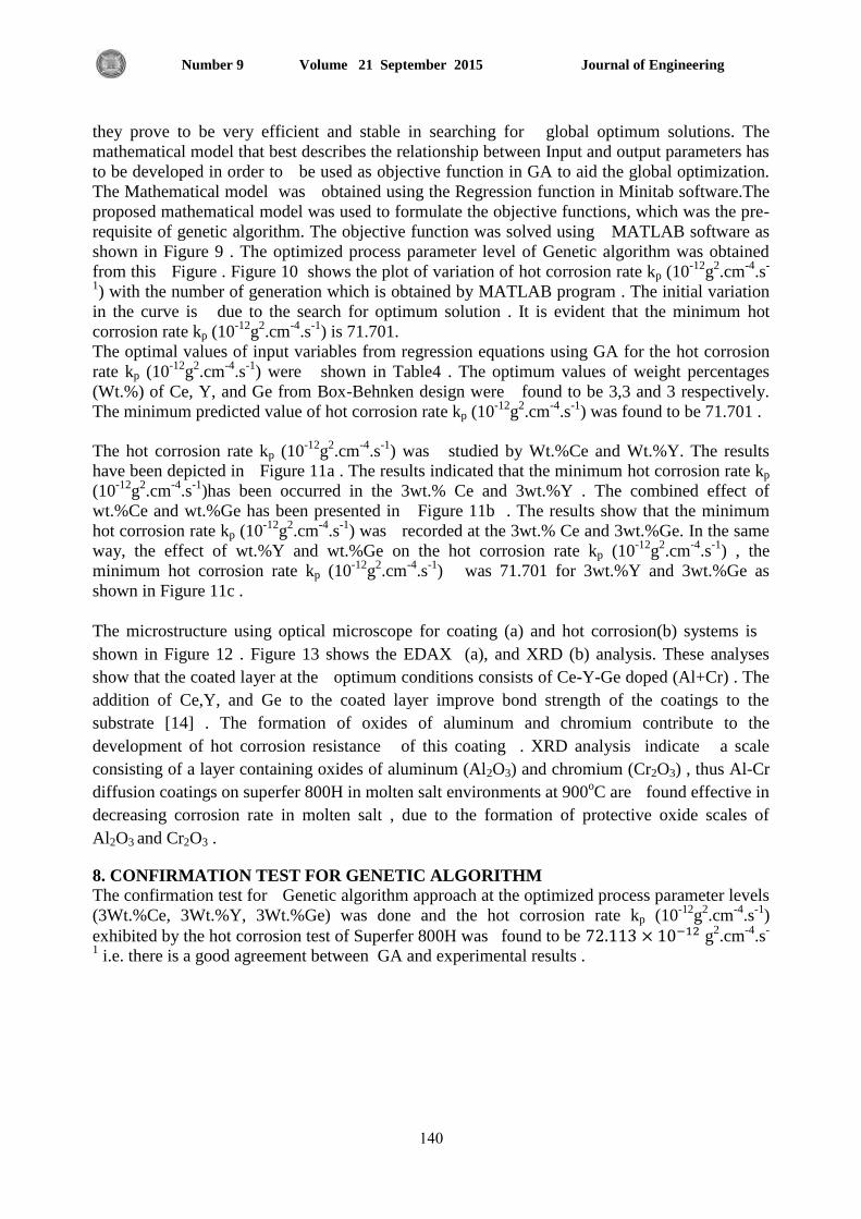
Journal of Engineering Volume 21 September 2015 Number 9
541
they prove to be very efficient and stable in searching for ط global optimum solutions. The
mathematical model that best describes the relationship between Input and output parameters has
to be developed in order to ط be used as objective function in GA to aid the global optimization.
The Mathematical model was ط obtained using the Regression function in Minitab software.The
proposed mathematical model was used to formulate the objective functions, which was the pre-
requisite of genetic algorithm. The objective function was solved using ط MATLAB software as
shown in Figure 9 . The optimized process parameter level of Genetic algorithm was obtained
from this ط Figure . Figure 10 shows the plot of variation of hot corrosion rate kp (10-12
g2.cm
-4.s
-
1) with the number of generation which is obtained by MATLAB program . The initial variation
in the curve is ط due to the search for optimum solution . It is evident that the minimum hot
corrosion rate kp (10-12
g2.cm
-4.s
-1) is 71.701.
The optimal values of input variables from regression equations using GA for the hot corrosion
rate kp (10-12
g2.cm
-4.s
-1) were ط shown in Table4 . The optimum values of weight percentages
(Wt.%) of Ce, Y, and Ge from Box-Behnken design were ط found to be 3,3 and 3 respectively.
The minimum predicted value of hot corrosion rate kp (10-12
g2.cm
-4.s
-1) was found to be 71.701 .
The hot corrosion rate kp (10-12
g2.cm
-4.s
-1) was ط studied by Wt.%Ce and Wt.%Y. The results
have been depicted in ط Figure 11a . The results indicated that the minimum hot corrosion rate kp
(10-12
g2.cm
-4.s
-1)has been occurred in the 3wt.% Ce and 3wt.%Y . The combined effect of
wt.%Ce and wt.%Ge has been presented in ط Figure 11b . The results show that the minimum
hot corrosion rate kp (10-12
g2.cm
-4.s
-1) was ط recorded at the 3wt.% Ce and 3wt.%Ge. In the same
way, the effect of wt.%Y and wt.%Ge on the hot corrosion rate kp (10-12
g2.cm
-4.s
-1) , the
minimum hot corrosion rate kp (10-12
g2.cm
-4.s
-1 was 71.701 for 3wt.%Y and 3wt.%Ge as ط (
shown in Figure 11c .
The microstructure using optical microscope for coating (a) and hot corrosion(b) systems is ط
shown in Figure 12 . Figure 13 shows the EDAX (a), and XRD (b) analysis. These analyses
show that the coated layer at the ط optimum conditions consists of Ce-Y-Ge doped (Al+Cr) . The
addition of Ce,Y, and Ge to the coated layer improve bond strength of the coatings to the
substrate [14] . The formation of oxides of aluminum and chromium contribute to the
development of hot corrosion resistance ط of this coating . XRD analysis indicate ط a scale
consisting of a layer containing oxides of aluminum (Al2O3) and chromium (Cr2O3) , thus Al-Cr
diffusion coatings on superfer 800H in molten salt environments at 900oC are ط found effective in
decreasing corrosion rate in molten salt , due to the formation of protective oxide scales of
Al2O3 and Cr2O3 .
8. CONFIRMATION TEST FOR GENETIC ALGORITHM
The confirmation test for ط Genetic algorithm approach at the optimized process parameter levels
(3Wt.%Ce, 3Wt.%Y, 3Wt.%Ge) was done and the hot corrosion rate kp (10-12
g2.cm
-4.s
-1)
exhibited by the hot corrosion test of Superfer 800H was ط found to be g2.cm
-4.s
-
1 i.e. there is a good agreement between GA and experimental results .
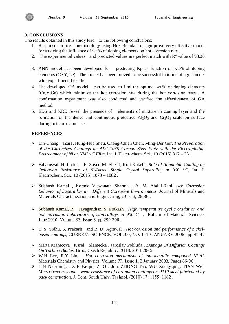
Journal of Engineering Volume 21 September 2015 Number 9
545
9. CONCLUSIONS
The results obtained in this study lead ط to the following conclusions:
1. Response surface ط methodology using Box-Behnken design prove very effective model
for studying the influence of wt.% of doping elements on hot corrosion rate .
2. The experimental values ط and predicted values are perfect match with R2 value of 98.30
.
3. ANN model has been developed for ط predicting Kp as function of wt.% of doping
elements (Ce,Y,Ge) . The model has been proved to be successful in terms of agreements
with experimental results.
4. The developed GA model ط can be used to find the optimal wt.% of doping elements
(Ce,Y,Ge) which minimize the hot corrosion rate during the hot corrosion tests . A
confirmation experiment was also conducted and verified the effectiveness of GA
method.
5. EDS and XRD reveal the presence of ط elements of mixture in coating layer and the
formation of the dense and continuous protective Al2O3 and Cr2O3 scale on surface
during hot corrosion tests .
REFERENCES
Lin-Chang ط Tsai1, Hung-Hua Sheu, Cheng-Chieh Chen, Ming-Der Ger, The Preparation
of the Chromized Coatings on AISI 1045 Carbon Steel Plate with the Electroplating
Pretreatment of Ni or Ni/Cr-C Film, Int. J. Electrochem. Sci., 10 (2015) 317 – 331.
Fahamsyah H. Latief, ط El-Sayed M. Sherif, Koji Kakehi, Role of Aluminide Coating on
Oxidation Resistance of Ni-Based Single Crystal Superalloy at 900 °C, Int. J.
Electrochem. Sci., 10 (2015) 1873 – 1882 .
Subhash Kamal , Korada Viswanath Sharma , A. M. Abdul-Rani, Hot Corrosion
Behavior of Superalloy in ط Different Corrosive Environments, Journal of Minerals and
Materials Characterization and Engineering, 2015, 3, 26-36 .
Subhash Kamal, R. س Jayaganthan, S. Prakash , High temperature cyclic oxidation and
hot corrosion behaviours of superalloys at 900°C , Bulletin of Materials Science,
June 2010, Volume 33, Issue 3, pp 299-306 .
T. S. Sidhu, S. Prakash س and R. D. Agrawal , Hot corrosion and performance of nickel-
based coatings, CURRENT SCIENCE, VOL. 90, NO. 1, 10 JANUARY 2006 , pp 41-47
.
Marta Kianicova , Karel س Slamecka , Jaroslav Pokluda , Damage Of Diffusion Coatings
On Turbine Blades, Brno, Czech Republic, EU18. 2011,20- 5 .
W.H Lee, R.Y Lin, ط Hot corrosion mechanism of intermetallic compound Ni3Al,
Materials Chemistry and Physics, Volume 77, Issue 1, 2 January 2003, Pages 86-96 .
LIN Nai-ming, , XIE Fa-qin, ZHOU Jun, ZHONG Tao, WU Xiang-qing, TIAN Wei,
Microstructures and ط wear resistance of chromium coatings on P110 steel fabricated by
pack cementation, J. Cent. South Univ. Technol. (2010) 17: 1155−1162 .

Journal of Engineering Volume 21 September 2015 Number 9
541
Bruce M. Warnes, Nick ط S. DuShane, Jack E. Cockerill, Cyclic oxidation of diffusion
aluminide coatings on cobalt base superalloys, Surface and Coatings Technology 148
(2001) 163–170.
A. ESLAMI, H. ARABI ط and S. RASTEGARI, Gas Phase Aluminizing Of A Nickel Base
Superalloy By A Single Step Htha Aluminizing Process, Canadian Metallurgical
Quarterly, Vol 48, No 1., 2009, pp 91-98.
I.M. Edmonds,, H.E. Evans, ط C.N. Jones, Oxidation & Coating Evolution In Aluminized
Fourth Generation Bladealloys, The mineral, metal materials society , superalloy2008,
pp.661-670.
H. R. Karimi Zarchi, M. ط Soltanieh, M. R. Aboutalebi, X. Guo2, Thermodynamic study
on pack aluminizing systems of pure titanium and nickel , Trans. Nonferrous Met. Soc.
China 23(2013) 1838−1846 .
Chao C. Jain ط and Chun H. Koo, Creep and Corrosion Properties of the Extruded
Magnesium Alloy Containing Rare Earth, Materials Transactions, Vol. 48, No. 2 (2007)
pp. 265 to 272.
Rajesh Ranjan ط Sinha, Dr. Brahm Deo Tripathi, Dr. Mahendra Yadav, Mines, Dhanbad,
Effect of rare earth additions on high-temperature oxidation resistance of V and Mo
alloyed steels, steel-grips.com 2013,pp.14-18.
Hongyu Wang , ط Dunwen Zuo, Gang Chen,, Guifang Sun ,, Xiangfeng Li,, Xu Cheng,
Hot corrosion behaviour of low Al NiCoCrAlY cladded coatings reinforced by nano-
particles on a Ni-base super alloy, Corrosion Science 52 (2010) 3561–3567.
Rober A.Rapp, Mark ط A.Haper and Robert Bianco, Codepostion elements by Halide
Activated Pack Cementation, JOM, Vol3, No.14,Nov.1991,pp.20-25.
Anderson ط and S.Ramachandran, A. Analysis of Corrosion at Hot Environment of
Plasma Sprayed Stainless Steels , European Journal of Scientific research, ISSN1450-
216X Vol.76 No.2 (2012) ط , pp. 300-308.
Douglas C.Montgomery ط , Design and Analysis of Experiments, John Wily &Sonc, Inc.,
2009 .
Daniel ط Graupe, Principles Of Artificial Neural Networks, 2nd Edition, World Scientific
Publishing Co. Pte. Ltd., 2007.
David A. Coley, ط An Introduction to Genetic Algorithms for Scientists and
Engineers,World Scientific Publishing Co. Pte. Ltd.1999.
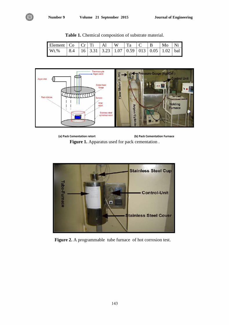
Journal of Engineering Volume 21 September 2015 Number 9
543
Table 1. Chemical composition of substrate material.
Element Co Cr Ti Al W Ta C B Mo Ni
Wt.% 8.4 16 3.31 3.23 1.07 0.59 013 0.05 1.02 bal
Figure 1. Apparatus used for pack cementation .
Figure 2. A programmable tube furnace of hot corrosion test.
(a) Pack Cementation retort (b) Pack Cementation Furnace

Journal of Engineering Volume 21 September 2015 Number 9
544
Table 2. Experimental design and results for hot corrosion rate kp (10-12
g2.cm
-4. s
-1)
Run Coded Values Actual Values kp (10-12
g2.cm
-4. s
-1)
X1 X2 X3 X1 X2 X3 observed Predicted
1 0 1 1 2 3 3 74.81 74.64
2 1 1 0 3 3 2 75.76 75.51
3 1 -1 0 3 1 2 77.65 77.46
4 0 1 -1 2 3 1 76.39 76.62
5 1 0 -1 3 2 1 80.55 80.57
6 -1 -1 0 1 1 2 81.19 81.44
7 -1 1 0 1 3 2 79.35 79.54
8 0 0 0 2 2 2 83.33 83.55
9 0 -1 -1 2 1 1 78.28 78.45
10 0 0 0 2 2 2 83.43 83.55
11 -1 0 1 1 2 3 82.7 82.68
12 1 0 1 3 2 3 77.04 77.46
13 -1 0 -1 1 2 1 83.76 83.34
14 0 -1 1 2 1 3 76.89 76.66
15 0 0 0 2 2 2 83.88 83.55
Table 3. Coded and actual values of variables of the experimental design
Factor Coded levels of variables
-1 0 +1
Wt.%Ce X1 1 2 3
Wt.%Y X2 1 2 3
Wt.%Ge X3 1 2 3
Figure 3. MINITAB session show the results of general regression.
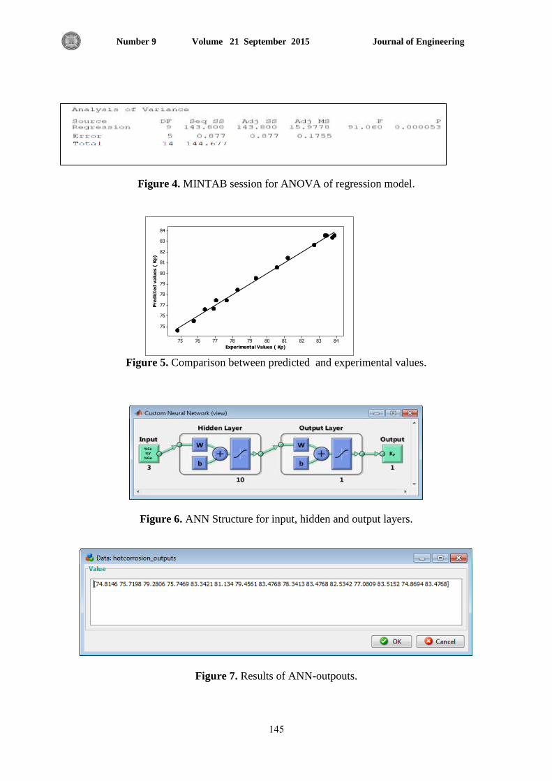
Journal of Engineering Volume 21 September 2015 Number 9
545
Figure 4. MINTAB session for ANOVA of regression model.
Figure 5. Comparison between predicted and experimental values.
Figure 6. ANN Structure for input, hidden and output layers.
Figure 7. Results of ANN-outpouts.
84838281807978777675
84
83
82
81
80
79
78
77
76
75
Experimental Values ( Kp)
Pre
dic
ted
va
lue
s (
Kp
)
%Ce%Y
%GeKP

Journal of Engineering Volume 21 September 2015 Number 9
546
Figure 8. Comparison of the experimentation and calculation.
Figure 9. Solver showing the results in MATLAB.
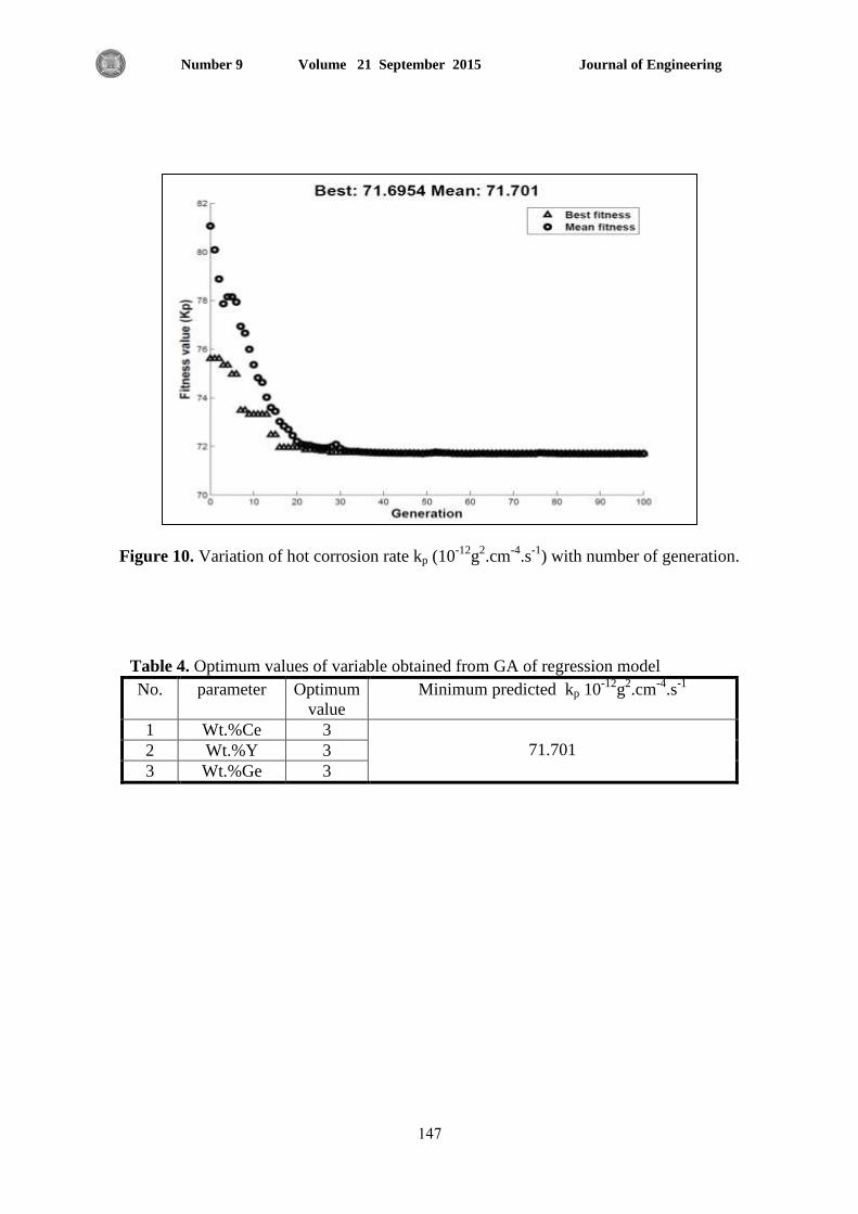
Journal of Engineering Volume 21 September 2015 Number 9
547
Figure 10. Variation of hot corrosion rate kp (10-12
g2.cm
-4.s
-1) with number of generation.
Table 4. Optimum values of variable obtained from GA of regression model
No. parameter Optimum
value
Minimum predicted kp 10-12
g2.cm
-4.s
-1
1 Wt.%Ce 3
71.701 2 Wt.%Y 3
3 Wt.%Ge 3
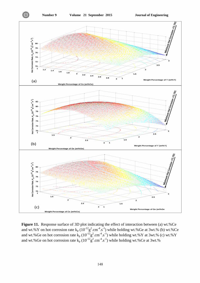
Journal of Engineering Volume 21 September 2015 Number 9
548
1
1.5
2
2.5
3 1
1.5
2
2.5
370
72
74
76
78
80
82
Weight Percentage of Y (wt%Y)
Weight Percentage of Ge (wt%Ge)
Ho
t C
orr
osi
on
Rat
e, K
P (
10-1
2 g2 .c
m-4
.s-1
)
1
1.5
2
2.5
3 1
1.5
2
2.5
3
70
72
74
76
78
80
Weight Percentage of Ge (wt%Ge
Weight Percentage of Ce (wt%Ce)
Ho
t C
orr
osi
on
Rat
e, K
P (
10-1
2 g2 .c
m-4
.s-1
)
11.2
1.41.6
1.82
2.22.4
2.62.8
3 1
1.5
2
2.5
3
70
72
74
76
78
80
Weight Percentage of Y (wt%Y)
Weight Percentage of Ce (wt%Ce)
Ho
t C
orr
osi
on
Rat
e, K
P (
10-1
2 g2 .c
m-4
.s-1
)
Min
imum
Hot
Cor
rosi
on =
71.7
01
Min
imum
Hot
Cor
rosi
on =
71.7
01
Min
imum
Hot
Cor
rosi
on =
71.7
01
(a)
(b)
(c)
Figure 11. Response surface of 3D plot indicating the effect of interaction between (a) wt.%Ce
and wt.%Y on hot corrosion rate kp (10-12
g2.cm
-4.s
-1) while holding wt.%Ge at 3wt.% (b) wt.%Ce
and wt.%Ge on hot corrosion rate kp (10-12
g2.cm
-4.s
-1) while holding wt.%Y at 3wt.% (c) wt.%Y
and wt.%Ge on hot corrosion rate kp (10-12
g2.cm
-4.s
-1) while holding wt.%Ce at 3wt.%

Journal of Engineering Volume 21 September 2015 Number 9
549
Al
Cl
Na
GeY
Ni
Cr
Ce
(a) (b)
Figure 12. The microstructure using optical microscope for coating (a) and hot corrosion(b)
systems
Figure 13. The EDAX (a), and XRD (b) analysis.
Superfer 800H
Oxi
de
-lay
er
Bas
e-M
eta
l
Al2O3+Cr2O3
(a)
100mSuperfer 800H
Ce-Y-Ge Doped Al-Cr
Bas
e-M
eta
lC
oat
ed
-Lay
er
100m
(b)

Journal of Engineering Volume 21 September 2015 Number 9
67
Performance Enhancement of a Piezoelectric Harvester Included into an
Autonomous System
Waleed Al-Ashtari
Instructor
College of Engineering - University of Baghdad
E-mail: [email protected]
ABSTRACT
Autonomous systems are these systems which power themselves from the available ambient
energies in addition to their duties. In the next few years, autonomous systems will pervade
society and they will find their ways into different applications related to health, security,
comfort and entertainment. Piezoelectric harvesters are possible energy converters which can be
used to convert the available ambient vibration energy into electrical energy. In this contribution,
an energy harvesting cantilever array with magnetic tuning including three piezoelectric bi-
morphs is investigated theoretically and experimentally. Other than harvester designs proposed
before, this array is easy to manufacture and insensitive to manufacturing tolerances because its
optimum operation frequency can be re-adjusted after fabrication. In this array, each bimorph has
its own rectification circuit in order to prevent the interference of its operation with the others.
Two electrical connections are investigated: the series connection and the parallel connection.
These connections are tested under several cases such as moderate and high excitation level and
large and small connected load. The theoretical and experimental works show that each connec-
tion has characteristics and can be used to enhance the harvester output power and/or its frequen-
cy bandwidth. These characteristics are highly related to the excitation level and the connected
load together.
Key words: piezoelectric bimorph, cantilever array, frequency tuning, electrical connections
تحسين اداء حاصذة كهروضغطية تستعمل لتىليذ الطاقة الكهربائية اللازمة لتشغيل جهاز راتي العمل
وليذ خالذ خيري الاشتري
هذسط
جبهعت بغذاد-ملت الذست
الخلاصة
حسخعول الطبقت الوجدة ف البئت الوحطت لخحلب ال الطبقت النشببئت اللاصهت الاجضة راحت العول حلل الاجضة الخ
ف السي القللت القبدهت, حلل الاجضة سخخفش بنزشة ف الوجخوع سجذ لب حطبقبث مزشة هخعلقت ببلصحت لاداء عولب.
خشغل ز الاجضة حذ وني لز الحبصذاث ححل احذ السبئل الوسخخذهت لالشفبت. الحبصذ اث لنشضغطت
عخببث الوصعت هي هاد مشضغطت. ححخ رلاد طبقت الاخضاص ال طبقت مشببئت. ف زا البحذ, حن حصون حبصذة
رببخت. مل عخبت وني حلف حشددب الطبع ببسخخذام هغبطمل عخبت حن حزبخب هي طشف احذ الطشف الاخش حشك حشا.
حوخبص ز الحبصذة الجذذة بب وني حجبص الخبرشث السلبت لسوبحبث الخصع بعذ حصعب رلل لا وني اعبدة حلف
الز عذ ححصذ امبش طبقت هونت. حن سبط لنل عخبت ف ز الحبصذة دائشة مشببئت حسخخذم لخحل الفلطت حشددب الاهزل
ال فلطت هسخوشة رلل لوع الخبرش السلب لنل عخبت مشضغطت عل الاخش. لقذ حن حصع ز الوخببت الوخلذة
الحبصذة دساسخب ظشب عولب.حن بحذ عي هي الشبط النشببئ لز العخببث النشضغطت: سبط عل الخال سبط
حوج دساسخوب عذ حسلط اخضاص ر سعت هخسطت عبلت عل الخاص. زاى الشبطبى حوج دساسخوب بعذة حبلاث هزلا
مشببئ صغش ا مبش. خبئج الظش العول بج ححسي مبش ف اداء الحبصذة الوقخشح هقبست هع مزلل عذ سبط حول
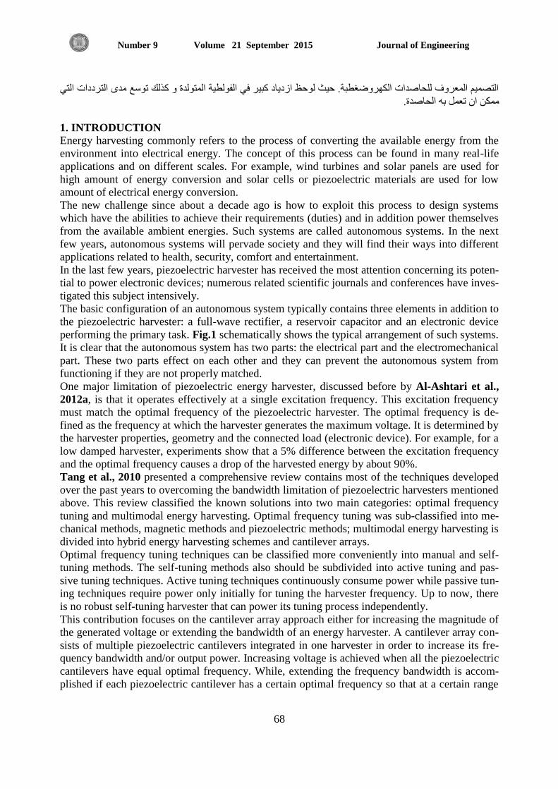
Journal of Engineering Volume 21 September 2015 Number 9
68
سع هذ الخشدداث الخ الخصون الوعشف للحبصذاث النشضغطبت. حذ لحظ اصدبد مبش ف الفلطت الوخلذة مزلل ح
حعول ب الحبصذة. ىهوني ا
1. INTRODUCTION
Energy harvesting commonly refers to the process of converting the available energy from the
environment into electrical energy. The concept of this process can be found in many real-life
applications and on different scales. For example, wind turbines and solar panels are used for
high amount of energy conversion and solar cells or piezoelectric materials are used for low
amount of electrical energy conversion.
The new challenge since about a decade ago is how to exploit this process to design systems
which have the abilities to achieve their requirements (duties) and in addition power themselves
from the available ambient energies. Such systems are called autonomous systems. In the next
few years, autonomous systems will pervade society and they will find their ways into different
applications related to health, security, comfort and entertainment.
In the last few years, piezoelectric harvester has received the most attention concerning its poten-
tial to power electronic devices; numerous related scientific journals and conferences have inves-
tigated this subject intensively.
The basic configuration of an autonomous system typically contains three elements in addition to
the piezoelectric harvester: a full-wave rectifier, a reservoir capacitor and an electronic device
performing the primary task. Fig.1 schematically shows the typical arrangement of such systems.
It is clear that the autonomous system has two parts: the electrical part and the electromechanical
part. These two parts effect on each other and they can prevent the autonomous system from
functioning if they are not properly matched.
One major limitation of piezoelectric energy harvester, discussed before by Al-Ashtari et al.,
2012a, is that it operates effectively at a single excitation frequency. This excitation frequency
must match the optimal frequency of the piezoelectric harvester. The optimal frequency is de-
fined as the frequency at which the harvester generates the maximum voltage. It is determined by
the harvester properties, geometry and the connected load (electronic device). For example, for a
low damped harvester, experiments show that a 5% difference between the excitation frequency
and the optimal frequency causes a drop of the harvested energy by about 90%.
Tang et al., 2010 presented a comprehensive review contains most of the techniques developed
over the past years to overcoming the bandwidth limitation of piezoelectric harvesters mentioned
above. This review classified the known solutions into two main categories: optimal frequency
tuning and multimodal energy harvesting. Optimal frequency tuning was sub-classified into me-
chanical methods, magnetic methods and piezoelectric methods; multimodal energy harvesting is
divided into hybrid energy harvesting schemes and cantilever arrays.
Optimal frequency tuning techniques can be classified more conveniently into manual and self-
tuning methods. The self-tuning methods also should be subdivided into active tuning and pas-
sive tuning techniques. Active tuning techniques continuously consume power while passive tun-
ing techniques require power only initially for tuning the harvester frequency. Up to now, there
is no robust self-tuning harvester that can power its tuning process independently.
This contribution focuses on the cantilever array approach either for increasing the magnitude of
the generated voltage or extending the bandwidth of an energy harvester. A cantilever array con-
sists of multiple piezoelectric cantilevers integrated in one harvester in order to increase its fre-
quency bandwidth and/or output power. Increasing voltage is achieved when all the piezoelectric
cantilevers have equal optimal frequency. While, extending the frequency bandwidth is accom-
plished if each piezoelectric cantilever has a certain optimal frequency so that at a certain range
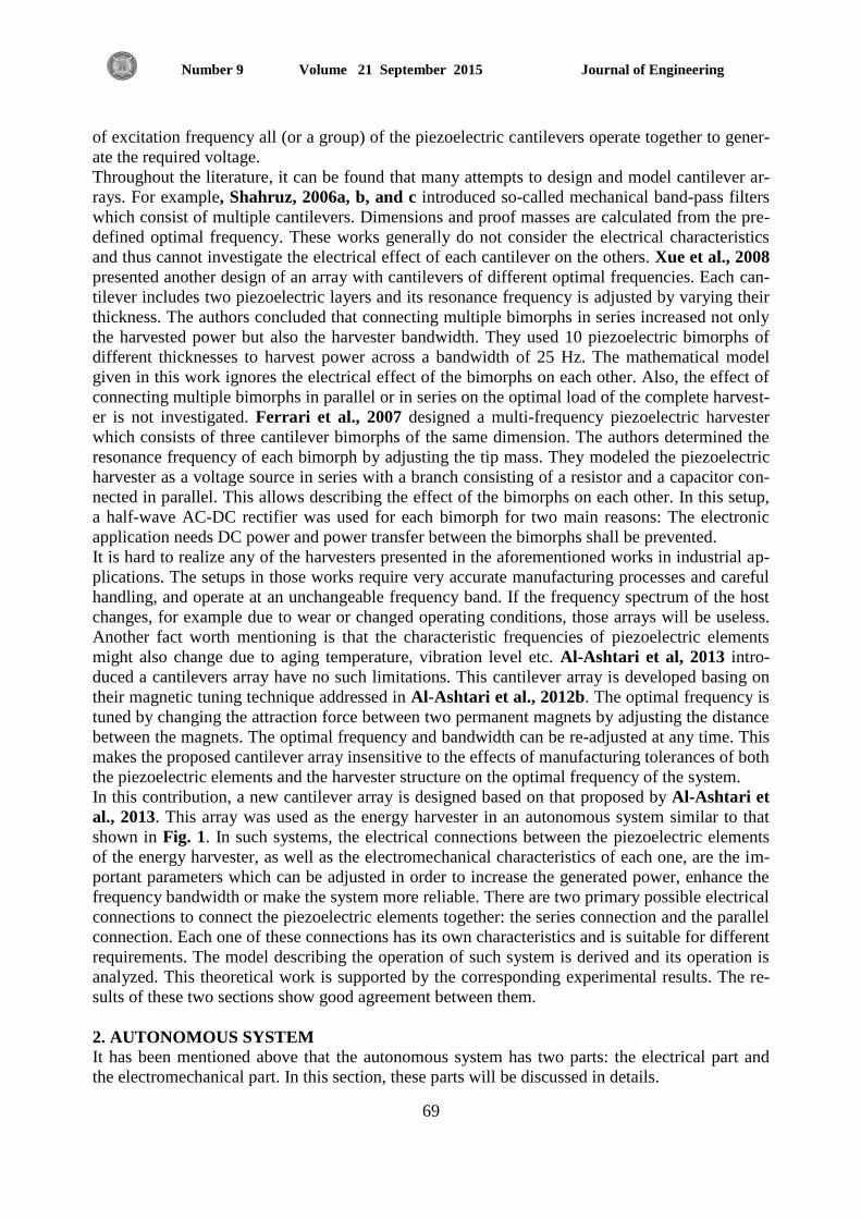
Journal of Engineering Volume 21 September 2015 Number 9
69
of excitation frequency all (or a group) of the piezoelectric cantilevers operate together to gener-
ate the required voltage.
Throughout the literature, it can be found that many attempts to design and model cantilever ar-
rays. For example, Shahruz, 2006a, b, and c introduced so-called mechanical band-pass filters
which consist of multiple cantilevers. Dimensions and proof masses are calculated from the pre-
defined optimal frequency. These works generally do not consider the electrical characteristics
and thus cannot investigate the electrical effect of each cantilever on the others. Xue et al., 2008
presented another design of an array with cantilevers of different optimal frequencies. Each can-
tilever includes two piezoelectric layers and its resonance frequency is adjusted by varying their
thickness. The authors concluded that connecting multiple bimorphs in series increased not only
the harvested power but also the harvester bandwidth. They used 10 piezoelectric bimorphs of
different thicknesses to harvest power across a bandwidth of 25 Hz. The mathematical model
given in this work ignores the electrical effect of the bimorphs on each other. Also, the effect of
connecting multiple bimorphs in parallel or in series on the optimal load of the complete harvest-
er is not investigated. Ferrari et al., 2007 designed a multi-frequency piezoelectric harvester
which consists of three cantilever bimorphs of the same dimension. The authors determined the
resonance frequency of each bimorph by adjusting the tip mass. They modeled the piezoelectric
harvester as a voltage source in series with a branch consisting of a resistor and a capacitor con-
nected in parallel. This allows describing the effect of the bimorphs on each other. In this setup,
a half-wave AC-DC rectifier was used for each bimorph for two main reasons: The electronic
application needs DC power and power transfer between the bimorphs shall be prevented.
It is hard to realize any of the harvesters presented in the aforementioned works in industrial ap-
plications. The setups in those works require very accurate manufacturing processes and careful
handling, and operate at an unchangeable frequency band. If the frequency spectrum of the host
changes, for example due to wear or changed operating conditions, those arrays will be useless.
Another fact worth mentioning is that the characteristic frequencies of piezoelectric elements
might also change due to aging temperature, vibration level etc. Al-Ashtari et al, 2013 intro-
duced a cantilevers array have no such limitations. This cantilever array is developed basing on
their magnetic tuning technique addressed in Al-Ashtari et al., 2012b. The optimal frequency is
tuned by changing the attraction force between two permanent magnets by adjusting the distance
between the magnets. The optimal frequency and bandwidth can be re-adjusted at any time. This
makes the proposed cantilever array insensitive to the effects of manufacturing tolerances of both
the piezoelectric elements and the harvester structure on the optimal frequency of the system.
In this contribution, a new cantilever array is designed based on that proposed by Al-Ashtari et
al., 2013. This array was used as the energy harvester in an autonomous system similar to that
shown in Fig. 1. In such systems, the electrical connections between the piezoelectric elements
of the energy harvester, as well as the electromechanical characteristics of each one, are the im-
portant parameters which can be adjusted in order to increase the generated power, enhance the
frequency bandwidth or make the system more reliable. There are two primary possible electrical
connections to connect the piezoelectric elements together: the series connection and the parallel
connection. Each one of these connections has its own characteristics and is suitable for different
requirements. The model describing the operation of such system is derived and its operation is
analyzed. This theoretical work is supported by the corresponding experimental results. The re-
sults of these two sections show good agreement between them.
2. AUTONOMOUS SYSTEM
It has been mentioned above that the autonomous system has two parts: the electrical part and
the electromechanical part. In this section, these parts will be discussed in details.

Journal of Engineering Volume 21 September 2015 Number 9
70
2.1 Electrical Part
In this paper the, behavior of an energy harvester connected to a rectifier circuit is introduced. As
shown in Fig. 2, the rectifier circuit consists of four diodes: , and . These diodes are
connected in the standard arrangement to convert the generated AC voltage from the harvester
into an output DC voltage .
Fig. 3a shows the generated AC voltage during the first two periods of operation, where
is the period. The corresponding output DC voltage is shown in Fig. 3b. These two figures show
that the first period of operation is very important and it includes four intervals; these intervals
are dependent on the design of the autonomous system components and their properties. Thus,
the autonomous system should be designed with this in mind to operate successfully. These in-
tervals are: the dead zone interval , the diode transient conduction interval , the open circuit
interval and finally the diode steady-state conduction interval .
The rectification process starts when the dead zone interval ends. This interval is defined as that
time interval during which the AC voltage is applied and there is no corresponding output DC
voltage. That’s because the input AC voltage amplitude is less than that required to overcome the
diode barrier voltage . The dead zone interval exists only in the first quarter of the first period
of operation (between 0 and ) as shown in Fig. 3b.
At the end of the dead zone interval , the transient conduction interval will start when the
amplitude of the generated AC voltage rises to be greater than the diodes’ barrier voltage. Within
this interval, either the first pair of diodes ( and ) is on and the other pair ( and ) is off
or vice-versa. This causes the current to flow from the harvester into the parallel loads and .
The size of the reservoir capacitor should be calculated carefully so that it will be is fully
charged at the end of this interval; otherwise the transient conduction time will continue over in-
to the next periods until the capacitor is fully charged. When the capacitor voltage rises higher
than the amplitude of generated AC voltage, the diodes will be off because the capacitor will try
to discharge its stored energy through them in their reverse direction.
This means the harvester is now disconnected from the load side i.e. it is in open-circuit condi-
tion. This will continue until the amplitude of the input AC voltage becomes greater than the ca-
pacitor voltage. This happens in a time interval called the open circuit interval . The load
in this interval is electrically powered only by the energy stored in the capacitor and the harvest-
er in open-circuit condition.
When the capacitor voltage becomes smaller than the amplitude of the applied AC voltage ,
then this interval will be ended and the steady-state conduction interval starts. Within this in-
terval, the other pair of diodes that were not conducting earlier will do so and the first conducting
pair will not. Within this time, the capacitor should be recharged.
The second and also all the next periods of operation have only the open circuit interval and the
diodes steady-state conductions intervals i.e. the system will be in its steady state operation as
shown in Fig. 3b.
In most real-life applications, the required charging time of the reservoir capacitor is much
smaller than required time for its discharging. This enables us to assume that almost all the gen-
erated current flows into the connected load during the diodes steady-state conductions intervals
i.e. during the steady state operation the harvester will serve two different loading conditions: the
open-circuit condition and resistive load condition. In this article, the connected load is chosen to
be large enough in order the generated voltages have almost the characteristics during these al-
ternative intervals.
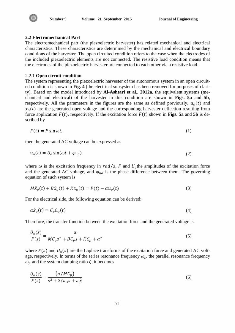
Journal of Engineering Volume 21 September 2015 Number 9
71
2.2 Electromechanical Part
The electromechanical part (the piezoelectric harvester) has related mechanical and electrical
characteristics. These characteristics are determined by the mechanical and electrical boundary
conditions of the harvester. The open circuited condition refers to the case when the electrodes of
the included piezoelectric elements are not connected. The resistive load condition means that
the electrodes of the piezoelectric harvester are connected to each other via a resistive load.
2.2.1 Open circuit condition
The system representing the piezoelectric harvester of the autonomous system in an open circuit-
ed condition is shown in Fig. 4 (the electrical subsystem has been removed for purposes of clari-
ty). Based on the model introduced by Al-Ashtari et al., 2012a, the equivalent systems (me-
chanical and electrical) of the harvester in this condition are shown in Figs. 5a and 5b,
respectively. All the parameters in the figures are the same as defined previously. and
are the generated open voltage and the corresponding harvester deflection resulting from
force application , respectively. If the excitation force shown in Figs. 5a and 5b is de-
scribed by
(1)
then the generated AC voltage can be expressed as
(2)
where is the excitation frequency in ⁄ , and the amplitudes of the excitation force
and the generated AC voltage, and is the phase difference between them. The governing
equation of such system is
(3)
For the electrical side, the following equation can be derived:
(4)
Therefore, the transfer function between the excitation force and the generated voltage is
(5)
where and are the Laplace transforms of the excitation force and generated AC volt-
age, respectively. In terms of the series resonance frequency , the parallel resonance frequency
and the system damping ratio , it becomes
( ⁄ )
(6)

Journal of Engineering Volume 21 September 2015 Number 9
72
Where,Al-Ashtari, 2012a
√
(7a)
(7b)
(
) (7c)
The generated AC voltage amplitude can be expressed as
( ⁄ )
√( )
(8)
and the phase difference is
(
) (9)
2.2.2 Resistive load condition
Resistive load condition refers to the condition in which the electrodes of the piezoelectric ele-
ment in a harvester are connected by a resistive load as shown in Fig. 6. All the parameters of
the systems are as defined previously. is the beam deflection from the external force
applied to the system. and are the corresponding generated voltage and charge
across the connected resistive load. Figs. 7a and 7b respectively show the equivalent mechanical
and electrical systems of a piezoelectric harvester at resistive load condition.
Now, the first goal is to calculate the generated voltage as a function of the connected load
and the excitation frequency , and then to derive the relationship between these two variables
in order to determine the condition at which the maximum power can be generated. The govern-
ing equation is the same as that for the open circuited condition, thus
(10)
for the mechanical side; for the electrical side, we have
(11)
and
(12)
As before, the transfer function between the excitation force and the generated voltage is

Journal of Engineering Volume 21 September 2015 Number 9
73
( ) ( ) (13)
In terms of series resonance frequency , parallel resonance frequency and damping ratio ,
which are defined by Eqs. (7a) ,(7b) and (7c), then Eq. (13) can be rewritten as
⁄
( ) ( )
(14)
This gives the amplitude of the generated AC voltage as
⁄
√[ ( ) ]
[ (
)]
(15)
and the phase difference is
( [ (
)]
( )
) (16)
Usually, a piezoelectric harvester is an electromechanical device that is located in or on a vibrat-
ing host structure to generate AC voltage, which can be used to power an electronic application.
Therefore, the base of the piezoelectric harvester is excited, thus exciting the entire structure.
The derived model can be valid if the force is replaced by the force . Where is the am-
plitude of the base acceleration. The generated DC voltage of a harvester in an autonomous
system can be expressed as
(17)
where is the generated voltage under conditions.
3. CANTILEVER ARRAY
There are two main connections can be used to connect electrically multiple piezoelectric ele-
ments: the series connection and the parallel connection. Also, each of these connections can be
performed by two different ways as will be shown later: direct connection and indirect connec-
tion.
3.1 Series Connection
The series connection of the piezoelectric elements can be classified into two types: the direct
and the indirect series connections.
3.1.1 Direct series connection
The direct series connection is when the electrodes of all the piezoelectric elements are connect-
ed together in series before the rectification process – for example, the system that is shown in
Fig. 8. For this connection, all the piezoelectric elements should have exactly the same optimal

Journal of Engineering Volume 21 September 2015 Number 9
74
frequency in order to gain an output voltage equal to the generated voltage of one element, times
the total number of elements (i.e., the ideal output).
If the harvester includes number of piezoelectric elements and all are excited by the applied
force , then the amplitude of the generated voltage by the element during steady-state
operation can be expressed as (based on Eq. (15))
⁄
√[ ( ) ]
[ (
)]
(18)
If all the elements have the same optimal frequency, then the amplitude of the total generated
voltage is
(19)
and the total output DC voltage can be calculated as
(20)
For this connection, if the piezoelectric elements have different optimal frequencies, then the
generated voltages of each one will have different amplitudes and be in different phases. This
will cause them to overlap and may lead to not achieving any enhancement.
3.1.2 Indirect series connection
The indirect series connection means that the piezoelectric elements in the harvester are connect-
ed together in series, but after the rectification process is carried out, as for example in the sys-
tem shown in Fig. 9.
If this harvester also includes number of piezoelectric elements, and these elements all have
small differences in their optimal frequencies, and if the excitation frequency matches the opti-
mal frequency of one piezoelectric element, then the other piezoelectric elements should be able
to generate voltage amplitudes equal to or more than that dropped through the diodes, so the total
DC voltage will be
∑
(21)
This connection can be used to expand the frequency bandwidth within which the harvester can
supply enough power to the connected load.
It is not practical to use the indirect connection if the piezoelectric elements have large differ-
ences in their optimal frequencies. That is because the losses of voltage across the diodes will be
very large. Thus, if a harvester includes number of piezoelectric elements, and is excited by a
harmonic acceleration of frequency that activates on piezoelectric element, which then generates
voltage while the others do not, then the total DC voltage at that case can be expressed as

Journal of Engineering Volume 21 September 2015 Number 9
75
∑[ ]
(22)
It seems to be that if a large number of piezoelectric elements are used then this may result in
there being no generated voltage anymore.
3.1.3 Tuning strategy for series connection
To achieve an expanded frequency bandwidth, each piezoelectric element should be tuned to a
different optimal frequency. The spread between the different frequencies defines the bandwidth
and the minimum voltage generated in this frequency range. In this paper, the tuning strategy is
developed so that at a frequency where two neighbouring piezoelectric elements generate the
same DC voltage, the voltage generated by each element is half the mean peak voltage of the two
elements.
Fig. 10 shows an example with three piezoelectric elements with approximately equal peak volt-
ages (the solid line curves). It is clear that these elements are tuned in such a way as to ensure
that at the frequencies and , the neighboring piezoelectric elements share equally in gen-
erating the total voltage. The total generated voltage is similar to that shown in Fig. 10 in the
dashed black line. It seems that the peak voltage that can be generated by a single piezoelectric
element at a single excitation frequency is extended across a considerable range as shown in Fig.
10.
This tuning strategy has been tested theoretically and experimentally, as will be shown later, and
the results show that this strategy is very effective for enhancing the frequency bandwidth of a
piezoelectric harvester.
3.2 Parallel Connections
If a harvester includes piezoelectric elements with different optimal frequencies which are
connected in parallel, then only the element that generates the higher voltage powers the load,
while the other elements do not. In a direct parallel connection, the other elements which are not
generating voltage at the moment behave as additional parallel loads. Therefore, these elements
cause the generated voltage to decrease. This is because these parallel elements reduce the
overall load connected to the operating element.
In indirect parallel connections, the voltage generated by the operating element prevents the
rectifier circuits of the other elements from conducting. Therefore, it is not advisable to use
either parallel connection type if the piezoelectric elements have different optimal frequencies.
If all the piezoelectric elements have the same optimal frequency and are connected in parallel
(direct or indirect), then the generated current increases. This case is not examined further
because it is interested in replacing batteries with piezoelectric harvesters in currently
commercial electronic applications. In such applications, achieving the required voltage is
necessary to ensure achieving of the required power for the operation; the current is therefore
uninteresting for this purpose.
4. EXPERIMENTAL VERIFICATION
Fig. 11 shows the experimental cantilever array harvester that was constructed to validate the an-
alytical model presented above. This harvester consists of three piezoelectric bimorphs (SITEX-
Module 427.0085.11Z from Johnson Matthey; specifications in Table 1). Magnetic stiffening Al-
Ashtari et al., 2012b can be used to tune each bimorph individually. The bimorphs are electri-
cally isolated from each other and from the aluminum base by plastic parts. Magnets with a face
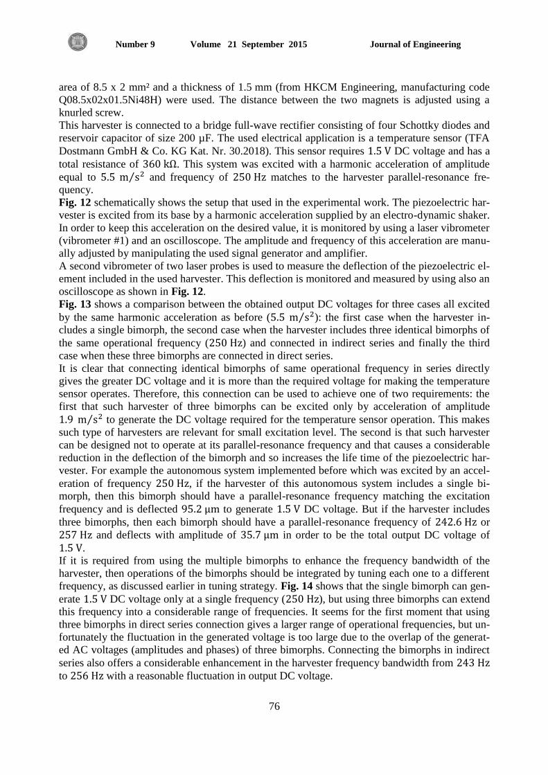
Journal of Engineering Volume 21 September 2015 Number 9
76
area of 8.5 x 2 mm² and a thickness of 1.5 mm (from HKCM Engineering, manufacturing code
Q08.5x02x01.5Ni48H) were used. The distance between the two magnets is adjusted using a
knurled screw.
This harvester is connected to a bridge full-wave rectifier consisting of four Schottky diodes and
reservoir capacitor of size 200 µF. The used electrical application is a temperature sensor (TFA
Dostmann GmbH & Co. KG Kat. Nr. 30.2018). This sensor requires DC voltage and has a
total resistance of . This system was excited with a harmonic acceleration of amplitude
equal to ⁄ and frequency of matches to the harvester parallel-resonance fre-
quency.
Fig. 12 schematically shows the setup that used in the experimental work. The piezoelectric har-
vester is excited from its base by a harmonic acceleration supplied by an electro-dynamic shaker.
In order to keep this acceleration on the desired value, it is monitored by using a laser vibrometer
(vibrometer #1) and an oscilloscope. The amplitude and frequency of this acceleration are manu-
ally adjusted by manipulating the used signal generator and amplifier.
A second vibrometer of two laser probes is used to measure the deflection of the piezoelectric el-
ement included in the used harvester. This deflection is monitored and measured by using also an
oscilloscope as shown in Fig. 12.
Fig. 13 shows a comparison between the obtained output DC voltages for three cases all excited
by the same harmonic acceleration as before ( ⁄ ): the first case when the harvester in-
cludes a single bimorph, the second case when the harvester includes three identical bimorphs of
the same operational frequency ( ) and connected in indirect series and finally the third
case when these three bimorphs are connected in direct series.
It is clear that connecting identical bimorphs of same operational frequency in series directly
gives the greater DC voltage and it is more than the required voltage for making the temperature
sensor operates. Therefore, this connection can be used to achieve one of two requirements: the
first that such harvester of three bimorphs can be excited only by acceleration of amplitude
⁄ to generate the DC voltage required for the temperature sensor operation. This makes
such type of harvesters are relevant for small excitation level. The second is that such harvester
can be designed not to operate at its parallel-resonance frequency and that causes a considerable
reduction in the deflection of the bimorph and so increases the life time of the piezoelectric har-
vester. For example the autonomous system implemented before which was excited by an accel-
eration of frequency , if the harvester of this autonomous system includes a single bi-
morph, then this bimorph should have a parallel-resonance frequency matching the excitation
frequency and is deflected to generate DC voltage. But if the harvester includes
three bimorphs, then each bimorph should have a parallel-resonance frequency of or
and deflects with amplitude of in order to be the total output DC voltage of
.
If it is required from using the multiple bimorphs to enhance the frequency bandwidth of the
harvester, then operations of the bimorphs should be integrated by tuning each one to a different
frequency, as discussed earlier in tuning strategy. Fig. 14 shows that the single bimorph can gen-
erate DC voltage only at a single frequency ( ), but using three bimorphs can extend
this frequency into a considerable range of frequencies. It seems for the first moment that using
three bimorphs in direct series connection gives a larger range of operational frequencies, but un-
fortunately the fluctuation in the generated voltage is too large due to the overlap of the generat-
ed AC voltages (amplitudes and phases) of three bimorphs. Connecting the bimorphs in indirect
series also offers a considerable enhancement in the harvester frequency bandwidth from
to with a reasonable fluctuation in output DC voltage.

Journal of Engineering Volume 21 September 2015 Number 9
77
5- CONCULSION
The feasibility of using harvester with multiple piezoelectric elements has been investigated. For
this purpose a cantilever array with three piezoelectric bimorphs was constructed to be used in
experimental verification. The results show good agreement between the theoretical and the ex-
perimental works. Strategies for connecting multiple bimorphs to increase the maximum gener-
ated power and/or enhance the bandwidth compared to a single bimorph harvester were also in-
vestigated.
The results show that the harvester with three bimorphs of identical optimal frequency can be
used either if the excitation amplitude is small or if it is required to generate higher voltage. The
result shows that the generated DC voltage of harvester with three bimorphs can be reached to
four times that generated of the harvester of single bimorph.
The results also show that using the proposed strategy of the optimal frequency tuning extends
the harvester frequency bandwidth considerably. The harvester of three bimorphs can generate
1.5 V DC for a range 13 Hz instead of generating this voltage at only single frequency.
ACKNOWLEDGMENT
The author gratefully acknowledge the support of Prof. Dr. Walter Sextro and the staff at the
Chair of Mechatronics and Dynamics / University of Paderborn.
REFERENCES
Al-Ashtari, W., Hunstig, M., Hemsel, T., and Sextro, W., 2012a, Analytical Determination of
Characteristic Frequencies and Equivalent Circuit Parameters of a Piezoelectric Bimorph, Jour-
nal of Intelligent Material Systems and Structures, Vol. 23, PP. 15-23.
Al-Ashtari, W., Hunstig, M., Hemsel, T., and Sextro, W., 2012b, Frequency Tuning of Piezoelec-
tric Energy Harvesters by Magnetic Force, Smart Mater. Struct., Vol. 21, PP. 035019.
Al-Ashtari, W., Hunstig, M., Hemsel, T., and Sextro, W., 2013, Enhanced Energy Harvesting Us-
ing Multiple Piezoelectric Elements: Theory and Experiments, Sensors and Actuators A, Vol.
200, PP. 138-146.
Ferrari, M., Ferrari, V., Guizzetti, M., Marioli, D., and Taroni, A., 2008, Piezoelectric Multifre-
quency Energy Converter for Power Harvesting in Autonomous Microsystems, Sensors and Actu-
ators A, Vol. 142 PP. 329-335.
Shahruz, S. M., 2006a, Design of Mechanical Band-Pass Filters for Energy Scavenging, J. Sound
and Vibration, Vol. 292, PP. 987-998.
Shahruz, S. M., 2006b, Design of Mechanical Band-Pass Filters with Large Frequency Bands for
Energy Scavenging, Mechatronics, Vol. 16, PP. 523-531.
Shahruz, S. M., 2006c, Limits of Performance of Mechanical Band-Pass Filters Used in Energy
Scavenging, J. Sound and Vibration, Vol. 293, PP. 449-461.

Journal of Engineering Volume 21 September 2015 Number 9
78
Tang, L., Yang, Y., and Soh, C. K., 2010, Toward Broadband Vibration-based Energy Harvest-
ing, J. Intelligent Material Systems and Structures, Vol. 21, PP. 1867-1896.
Xue, H., Hu, Y., and Wang, Q., 2008, Broadband Piezoelectric Energy Harvesting Devices Using
Multiple Bimorphs with Different Operating Frequencies, IEEE Transactions on Ultrasonics, Fer-
roelectrics and Frequency Control, Vol. 55, PP. 2104-2108.
NOMENCLATURE
= equivalent mechanical damping of a piezoelectric device, ⁄
= equivalent capacitance of the piezoelectric material,
= reservoir capacitor,
= applied excitation force,
= frequency at which piezoelectric element generates maximum voltage,
= frequency at which piezoelectric element generates half maximum voltage,
= equivalent mechanical stiffness of a piezoelectric device, ⁄
= total equivalent mass of a piezoelectric device,
= number of used piezoelectric elements included in the harvester
= generated charge of the piezoelectric harvester at resistive load condition,
= connected Resistive load,
= time,
= period
= dead zone interval,
= transient conduction interval,
= steady-state interval,
= open circuit interval,
= diode drop barrier voltage,
= amplitude of the total generated voltage of a harvester included multiple piezoelectric el-
ements connected directly in series,
= amplitude of the generated voltage of the piezoelectric element at resistive load condi-
tion,
= amplitude of the generated voltage at open circuit condition,
= generated AC voltage of the piezoelectric harvester at open circuit condition,
= generated AC voltage of the piezoelectric harvester at resistive load condition,
= generated DC voltage of a harvester included multiple piezoelectric elements connected
directly in series,
= generated DC voltage of a harvester included multiple piezoelectric elements connected
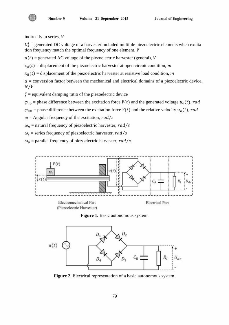
Journal of Engineering Volume 21 September 2015 Number 9
79
indirectly in series,
= generated DC voltage of a harvester included multiple piezoelectric elements when excita-
tion frequency match the optimal frequency of one element,
= generated AC voltage of the piezoelectric harvester (general),
= displacement of the piezoelectric harvester at open circuit condition,
= displacement of the piezoelectric harvester at resistive load condition,
= conversion factor between the mechanical and electrical domains of a piezoelectric device,
⁄
= equivalent damping ratio of the piezoelectric device
= phase difference between the excitation force and the generated voltage ,
= phase difference between the excitation force and the relative velocity ,
= Angular frequency of the excitation, ⁄
= natural frequency of piezoelectric harvester, ⁄
= series frequency of piezoelectric harvester, ⁄
= parallel frequency of piezoelectric harvester, ⁄
Figure 1. Basic autonomous system.
Figure 2. Electrical representation of a basic autonomous system.
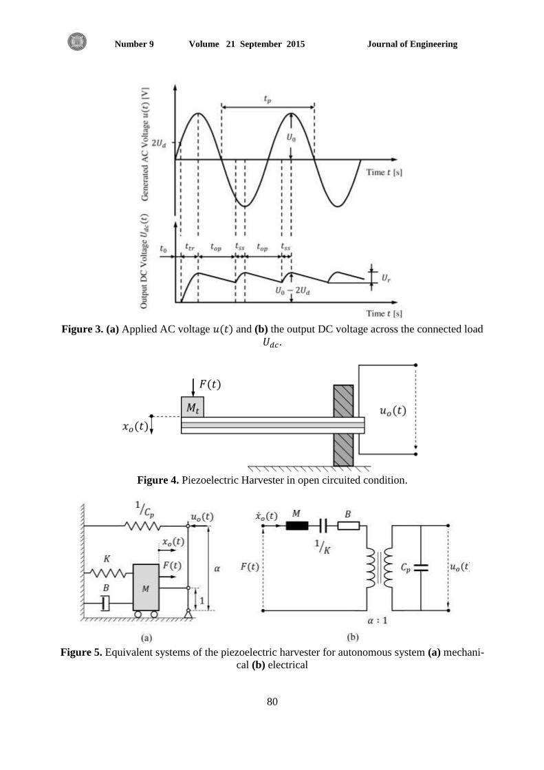
Journal of Engineering Volume 21 September 2015 Number 9
80
Figure 3. (a) Applied AC voltage and (b) the output DC voltage across the connected load
.
Figure 4. Piezoelectric Harvester in open circuited condition.
Figure 5. Equivalent systems of the piezoelectric harvester for autonomous system (a) mechani-
cal (b) electrical

Journal of Engineering Volume 21 September 2015 Number 9
81
Figure 6. Piezoelectric harvester connected to a resistive load.
Figure 7. Equivalent systems of piezoelectric harvester connected to resistive load (a) mechani-
cal and (b) electrical.
Figure 8. Autonomous system including a harvester with two piezoelectric elements connected
in direct series.

Journal of Engineering Volume 21 September 2015 Number 9
82
Figure 9. Autonomous system including a harvester with two piezoelectric elements connected
in indirect series.
Figure 10. Tuning strategy for bandwidth enhancement.
Figure 11. Experimental rig showing a cantilever array of three piezoelectric bimorphs.
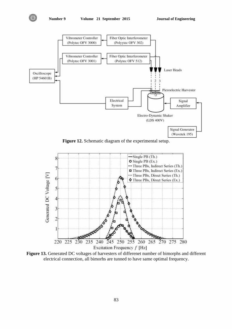
Journal of Engineering Volume 21 September 2015 Number 9
83
Figure 12. Schematic diagram of the experimental setup.
Figure 13. Generated DC voltages of harvesters of differenet number of bimorphs and different
electrical connection, all bimorhs are tunned to have same optimal frequency.
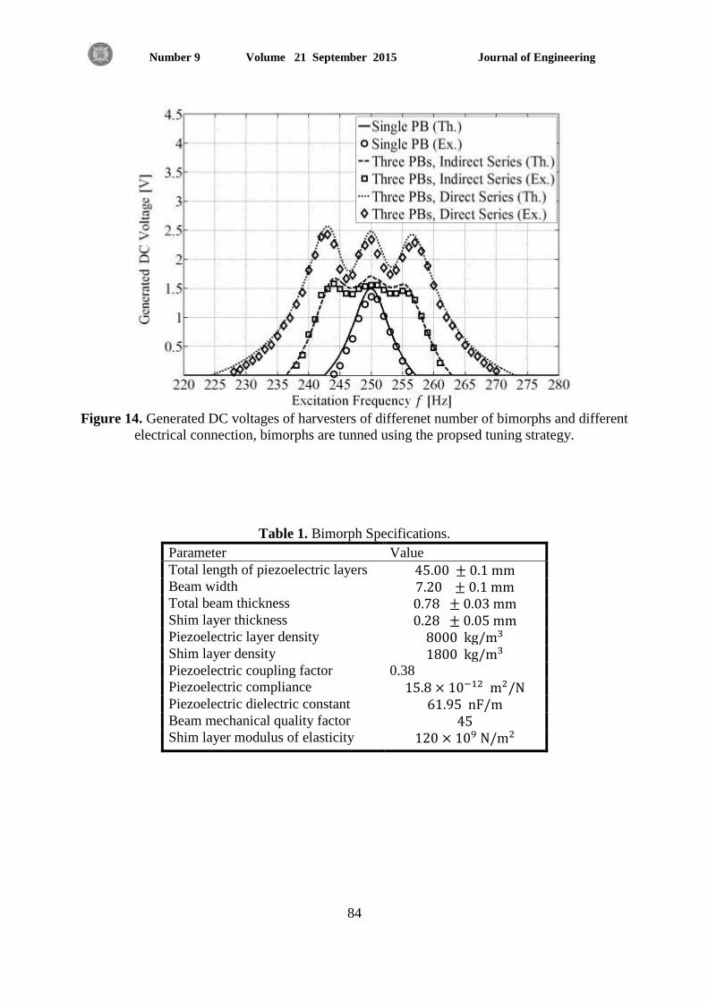
Journal of Engineering Volume 21 September 2015 Number 9
84
Figure 14. Generated DC voltages of harvesters of differenet number of bimorphs and different
electrical connection, bimorphs are tunned using the propsed tuning strategy.
Table 1. Bimorph Specifications.
Parameter Value
Total length of piezoelectric layers Beam width Total beam thickness Shim layer thickness Piezoelectric layer density Shim layer density Piezoelectric coupling factor 0.38
Piezoelectric compliance Piezoelectric dielectric constant Beam mechanical quality factor Shim layer modulus of elasticity

Journal of Engineering Volume 21 September 2015 Number 9
105
Reduction of Noise and Vibration of Spur Gear by Using Asymmetric Teeth
Profiles with Tip Relief
Mohammad Qasim Abdullah Adnan Naji Jameel
Professor Professor
Engineering College, University of Baghdad Engineering College, University of Baghdad
Email:[email protected] Email: [email protected]
Husam Saad Hasan
PHD Student
Engineering College, University of Baghdad
Email:[email protected]
ABSTRACT
Reduction of noise and vibration in spur gear experimentally by using asymmetric teeth
profiles with tip relief was presented. Both of classical (symmetric) and asymmetric (with and
without tip relief) spur gears are used in this work. Gear test rig was constructed to achieve
torsional vibration measuring, and two modified cutters are designed and manufactured to
achieve tooth profile modifications. First to cut asymmetric gear tooth with pressure angles
(14.5o/25
o) without tip relief for loaded and unloaded tooth sides respectively, and second to cut
asymmetric gear tooth with pressure angles (14.5o/25
o) for loaded and unloaded tooth sides
respectively with tip relief to achieve best dynamic performance. Dynamic load factor,
transmission error and noise level are carried out in this work. Final results showed improvement
in dynamic load factor and noise level for asymmetric gear (with and without tip relief)
compared with classical spur gear .
Key words: dynamic load factor, tooth transmission error, asymmetric tooth profile , tooth tip
relief.
للمسننات العدلة بواسطة جانبيات الاسنان غير المتناضرة مع تشذيب اختزال الضوضاء والاهتزاز
الحواف
هحود قاسن عبد الله عداى اجي جويل
اسخار اسخار
خايعت بغذاد /كهيت انهذست خايعت بغذاد / كهيت انهذست
حسام سعد حسي
طانب دكخىساة
خايعت بغذاد / كهيت انهذست
الخلاصة
اخخضال انضىضاء والاهخضاص نهساث انعذنت عهيا بىاسطت اسخخذاو خابياث اسا غيش يخاضشة يع حشزيب حى حقذيى
حى اسخخذايه في هزا حشزيب انحىاف وبذوها( في هزا انبحث. كلا ي الاسا انخاضشة وانغيش يخاضشة ) يع انحىاف
يصت اخخباس انساث بيج خصيصا نخحقيق قياط الاهخضاص انذوساي وحى حصيى وحصيع قاطعاث يساث يحىسة .انعم
وانثايت بذو حشزيب انحىاف. دسخت ( 14.5/25اظش رو صوايا ضغظ )نخحىيش خابياث الاسا. الاون نقطع يس غيش يخ
دسخت رو خاصيت عه حشزيب حىاف انس ورنك نضا افضم اداء ( 14.5/25رو صوايا ضغظ )نقطع يس غيش يخاضش

Journal of Engineering Volume 21 September 2015 Number 9
106
انخائح انهائيت .دياييكي . في هزا انبحث حى اسخخشاج يعم انحم انذياييكي وخطا انقم انذياييكي ويسخىي انضىضاء
زيب نحافاث شغيش انخاضشة ) بىخىد وعذو وخىد حاظهشث ححسي في يعم انحم انذياييكي ويسخىي انضىضاء نهساث
الاسا ( يقاست بالاسا انخقهيذيت .
.: يعايم انحم انذياييكي , خطأ انقم نس انس ,اسا غيش يخاضشة اندابياث , حشزيب حىاف الاسا الكلوات الرئيسية
1. INTRODUCTION Dynamic loads, vibration and noise level have been considered as a major problem in
transmitting machines especially at high speeds and heavy loads .Tooth transmission error
(Tm) and non linear mesh stiffness have been represented a major excitation sources for
vibration and noise in gear drive system, as the tooth transmission error defined as the
difference between actual and ideal position of driven gear . The aim of this paper is
reducing of dynamic load factors, transmission error and noise level by modifying gear tooth
profiles experimentally by using asymmetric teeth profiles with tip relief, where relief
defined as removing metal from the tip or the root of the teeth or from both, Smith, 1999.
Little literature attempted to investigate dynamic characteristics of spur gear system
experimentally. Munro, 1962 measured dynamic transmission error in spur gear pair, he
selected high precision spur gears with manufacturing errors much smaller than tooth
deflection, and he applied tooth profile modifications to achieve minimum static
transmission error at design load. Kubo, 1962 designed gear test rigs which were heavily
damped, he measured dynamic root stress and then estimated the dynamic factor. Smith,
1999 used two smaller optical rotary encoder made by Heidenhain Ltd. which had
become readily available and used extensively for rotary positioning system on tooth
geared system. His results indicated error below 0.1 second of arc at operating speed. Kang
,2009 indicted the shaft compliance effect on dynamic Tranmission error, he used
tangential accelerometer for measuring the gear motions in rotational, torsional and
translitional axis, he used spur and helical gears in his experimental work. In this work
gear test rig was built to achieve torsional vibration measuring, and two modified cutters
was designed and manufactured to achieve tooth profile modifications such as asymmetric
tooth profile with and without tip relief to improve dynamic load factor, transmission error
and noise level.
2. PROBLEM FORMULATION Simple dynamic model with single degree of freedom has been employed in this work
;therfore , equation of motion will be, Hasan, et al,2014 :
(1)
Where x(t) refers to dynamic transmission error of a gear pair along its line of action which
defined as:
(2)
represented base radius for pinion and gear respectively , represented
angular displacement for gear and pinion respectively, and e(t) represented periodic static
transmission error , me equivalent mass, km non linear mesh stiffness , cm non linear mesh
damping and F static load .
Dynamic load factor in gear drive system defined as the ratio of dynamic mesh load to static
load under operating speed :
(3)
Dynamic mesh load in Eq. (3) defined as, Duboswky and Freudenstein, 1971:
Journal of Engineering Volume 21 September 2015 Number 9
107
(4)
Sub. Eq. (4) in Eqs. (1) and (3). Dynamic load factor has been written in terms of second
derivative of transmission error as:
(5)
Where ( & ) measured by gear test rig experimentally as shown in next section .
3. GEAR TEST RIG Test rig was constructed to analyze dynamic performance in gear drive system such as
dynamic load factor, transmission error and noise level. Three types of steel spur gear pairs with
a unity speed ratio (1:1) and a fixed center distance of 98 mm had been selected to be under the
test. The first type was symmetric spur gear with classical pressure angles (20 o
/20 o
). The second
type was asymmetric spur gear with pressure angles (14.5o/25
o) for loaded and unloaded tooth
sides respectively. Third type was asymmetric spur gear with pressure angles (14.5o/25
o) for
loaded and unloaded tooth sides respectively but with tip relief. All design parameters of the
symmetric and asymmetric spur gear drives with and without tip relief are listed in table (1). The
chemical composition of the spur gears (pinion and gear) and shafts material are inspected in
“Specialized Institute for Engineering Industries/Ministry of Industry & Minerals/Iraq” that was
listed in Appendix (A) .
A gear milling operation had been adopted to manufacture the test specimens (prototypes) of all
spur gears by using standard and modified gear milling cutters.
A standard HSS gear milling cutter of disc type had been adopted to cut symmetric prototypes
of spur gears (pinion and gear). According to the design specifications of DIN 3972, the cutter
number can be selected by depending on the gear design parameters to be cut, where each cutter
number was designed to cut a range of teeth number for certain pressure angle and module,
therefore; with gear design parameters , 7 mm and 14 teeth, cutter No.2 in
Appendix (B) had been selected, where this cutter can be used to cut three gears with different
number of teeth ( 14, 15 and 16 teeth) .
A modified HSS gear milling cutter of disc type with asymmetric involute profiles with
optimal fillet radii and without tip relief had been designed by Abdullah and Jweeg, 2012,
depending on the tooth profiles geometry. Asymmetric tooth profiles with tip relief had been
design depending on reduction in static transmission error by selecting appropriate amount and
location of tip relief on asymmetric tooth profile ( tip amount 40 micron , start relief lied on 0.33
base pitch on involute profile ) as shown in Fig.1 ,amount and extent of tip relief achieved
theoretical basis of spur gear profile relief design that established by Munro et ,al ,1990 and
palmer ,1999 .
The workshop drawings and manufacturing of these cutters had been achieved by “Acedes Gear
Tools Company (division of Furzeland Ltd.) / UK-England”. Final products of these cutters are
shown in Fig.2. Test rig (gear-shaft-bearing system) as shown in Fig.3 had been constructed
precisely to indicate dynamic load factor, transmission error and noise level under certain
external load and rotational speed values for symmetric , asymmetric and asymmetric with tip
relief spur gear . Two steel gears (pinion and gear) of the same diameter of 98 mm are fixed on
two steel shafts with diameter of 49 mm; where two ball bearings supported each shaft. AC
motor ( 3 KW, 2880 rpm, Three-phases, 220~230 Volt, 50~60 Hz, MeZ Electric Motors
Ltd./Czech Rep.) was used to provide sufficient amounts of the required torque to overcome the
overall inertias of mechanical components of test rig and steel flywheels with masses ( 5 kg , 15
kg , 25kg , 35 kg ) respectively. Speed control was automated by using a controller speed device

Journal of Engineering Volume 21 September 2015 Number 9
108
(Variable Frequency Drive , Power range: from 0.4 to 3.75 KW, Three phase, 220~230 Volts,
50~60 Hz, Delta Industrial Systems Co. Ltd./ Taiwan) . A thick steel plate with dimensions (700
300 20 mm) was used as a platform for fixing the motor by using four bolts with diameter
of 10 mm and the fixed four housings by using four bolts with diameter of 12 mm for each
housing. The measurement system was designed to perform measuring torsional vibration
components (θ1 and θ2 ) for both pinion and gear. Uni-axial tangential accelerometer was
devised. Accelerometers (PCB Piezotronics, Model: 353B18, sensitivity: nearly 10 mV/g,
frequency range: 0 to 10 kHz) can be mounted tangentially at pinion and gear respectively as
shown in Fig4.
The accelerometers data are fed to the fixed frame through the end-of-shaft by using slip
rings (Jinapat SR, Model: LPT038). Signals transmitted from the slip rings are fed into a multi-
channel signal conditioner (PCB Piezotronics ICP Model 482C64) to condition and amplify the
data. Then, the signals are fed to Digital storage Oscilloscope that digitizes the analog signals at
a user defined sampling rate and monitoring signals in voltage amplitudes, Fig. 5 shows the flow
chart for measurement system .
Sound intensity levels can be measured by using a sound level meter (Model: SL-4022, IEC
61672 class 1, Microphone type: Electrical condenser, Measurement range: from 30 to 130 dB,
Lutron Electronic Enterprice Co. Ltd./Taiwan) by putting meter microphone vertically with a
distance 15 Cm above the gears engagement location to obtain purest sound signal as shown in
Fig. 6 .
4. RESULTS AND DISCUSSION
Digital storage oscilloscope shows accelerometers signals, but in voltage amplitudes, so these
data should be converted to acceleration values in (m/s2) by using accelerometer conversion
scale. Dynamic transmission error defined as the difference between axial displacement of pinion
and gear ; therefore, Sigview software (V 2.6) analyzed storage signals and integrated it twice
to carry out dynamic transmission error and dynamic load factor.
Fig. 7 shows the variation of noise levels (sound intensity level in dB) with rotational speed of
motor for both of asymmetric gear teeth with and without tip relief. Generally Tip relief in
asymmetric gear teeth reduced the noise levels of spur gear by around (10 -20) % in low
speeds (less than 1000 rpm ) and by around (2 -5 ) % in high speeds ( more than 3000 rpm ).
Fig.8 shows dynamic load factors with rotational speed of motor for symmetric gear teeth with
pressure angles (20 o
/20 o
) and asymmetric gear teeth with pressure angles (14.5 o
/25 o
) without
tip relief . Generally asymmetric gear tooth with tip relief shows improvement in dynamic load
factors at all speeds except at super harmonic frequency which occurred at 1000 rpm .In high
speeds ( more than 2000 rpm) the dynamic load factor became greater compared with low speeds
and symmetric gear tooth recorded high peak of dynamic load factor at 2200 rpm which
approximate 6 for dynamic load factor .
Fig. 9 shows comparison between dynamic load factors with rotational speed of motor for
asymmetric tooth gear with and without tip relief , this figure shows convergence in results but
with improvement for asymmetric tooth without tip relief at low speeds ( less than 1000 rpm )
and improvement for asymmetric tooth with tip relief at high speeds ( more than 1200 rpm ) .
Fig. 10 shows the effect of different inertial loads on dynamic load factors for asymmetric gear
tooth with tip relief. (5kg, 15 kg and 25 Kg) fly wheels are used in gear test rig. In low speeds
(less than 1500 rpm) both of (5 and 25 kg ) flywheels showed improvement in dynamic load
factors compared with 15 kg flywheel . In high speeds (more than 1500 rpm) 15 kg flywheel
showed improvement in dynamic load factors compared with 25 kg flywheel which was
increased while 5kg inertia still better compared with both of (15 &25 kg) flywheels.

Journal of Engineering Volume 21 September 2015 Number 9
109
Fig. 11 shows dynamic load factors for symmetric gear tooth with loaded pressure angle (200)
and asymmetric gear tooth with tip relief and loaded pressure angle (250) with rotation speed .
Results showed improvement by around (51%) in asymmetric gear tooth at most speeds (higher
than 500 rpm) although loaded pressure angle in symmetric gear tooth lower than asymmetric
gear (250) due to modified loaded tooth side by medium tip relief.
Fig.12 shows dynamic transmission error for symmetric and asymmetric tooth gear with
rotation speed, it's clear that asymmetric gear tooth showed improvement by around (50 %) in
dynamic transmission error compared with symmetric tooth gear at all speeds except (1000
rpm) .
Fig. 13 shows improvement by around ( 50%) in dynamic transmission error for asymmetric
gear tooth without tip relief compared with asymmetric gear tooth with tip relief at low speeds
(less than 1100 rpm ) ,for other speeds tip relief modification in asymmetric tooth profile
improve dynamic transmission error in spur gear by around (20-66 %) .
Fig. 14 shows the effect of different inertias on dynamic transmission error for asymmetric
tooth gear with tip relief , and three regions were remarked in this figure. In low speeds (less
1000 rpm) (5kg and 25 kg) flywheels showed improvement in results compared with 15 kg
flywheel , at speeds ( 1000 -2000 rpm) (15kg and 25 kg ) flywheels show improvement in
results compared with 5 kg flywheel , at high speed ( more than 2000 rpm ) 15 kg flywheel
shows improvement in results compared with ( 5 kg and 25 kg) flywheels .
Table 2 showed maximum dynamic load factors and maximum dynamic transmission errors that
were recorded in previous figures.
5. CONCLUSION Noise level, Dynamic load factor and dynamic transmission error are carried out
experimentally in this paper. Results showed that the noise radiated from asymmetric gear drive
system was improved when asymmetric profiles modified by appropriate tip relief by around
(10 -20) % in low speeds and by around (2 -5) % in high speeds .
Asymmetric gear teeth with and without tip relief showed improvement in dynamic load factor
and dynamic transmission error compared with symmetric gear tooth where percentage
improvement reach (50 – 80) % in different rotations speed. Minimum flywheel (5 kg) used in
asymmetric gear drive showed lowest dynamic load factor compared with other flywheels
while (15) kg flywheel showed lowest dynamic transmission error compared with other
flywheels.
REFRENCES
Abdullah ,M.Q., and Jweeg ,M.J. ,2012, Simulation of Generation Process for Asymmetric
Involute Gear Tooth Shape with and without Profile Correction, Innovative Systems Design
and Engineering , Vol.3 ,No. 6 ,pp19-35.
Duboswky S., and Freudenstein F., 1971, Dynamic Analysis of Mechanical Systems with
Clearance Part1and Part 2 ", ASME journal of Engineering for Industrial, pp 305 – 306.
Husam, S. H. , Adnan ,N. J. , and Abdullah , M. Q. , 2014, A Novel Method for Evaluating
The Dynamic Load Factor of An Involute Tooth Gear with Asymmetric Profiles , Innovative
Systems Design and Engineering ,Vol. 5 , No.10 , pp 17-30.
Kubo, A., Yamada, K., Aida, T. and Sato S., 1972, Research on Ultra High Speed Gear
Devices (reports 1-3) ,Transactions of Japanese Society of Mechanical Engineers 38, 2692-
2715.

Journal of Engineering Volume 21 September 2015 Number 9
110
Kang , Ma Ru , 2009, Measurement of Vibrations of Gears Supported by Compliant
Shafts, MS.C Thesis , university of ohio state .
-Munro, R. G, 1962, The Dynamic Behavior of Spur Gears, Ph. D. Dissertation,
Cambridge University.
-Munro, R.G., Yildirim, N. , and Hall, D.M.1990, Optimum Profile Relief and
Transmission Error in Spur Gears, I Mech E Conference on Gearbox Noise and
Vibration, Paper C404/032, 35–41.
-Palmer D., 1999,The Effects of Profile Relief on Narrow Face Width Parallel Axis
Gears, Ph.D. Dissertation, Huddersfield University.
- Smith J.D., 1999, Gear Noise and Vibration, by Marcel Dekker Inc., New York, USA
, 1st Edition.
Figure 1 . Asymmetric tooth profile with tip relief.
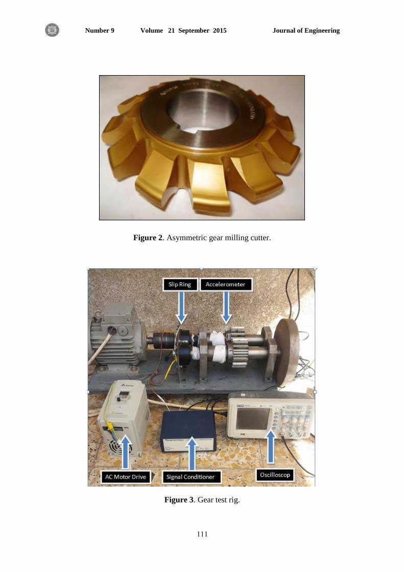
Journal of Engineering Volume 21 September 2015 Number 9
111
Figure 2. Asymmetric gear milling cutter.
Figure 3. Gear test rig.

Journal of Engineering Volume 21 September 2015 Number 9
112
Figure 4. Tangential accelerometer.
Figure 5 . Noise measurement .
Icp accelerometer
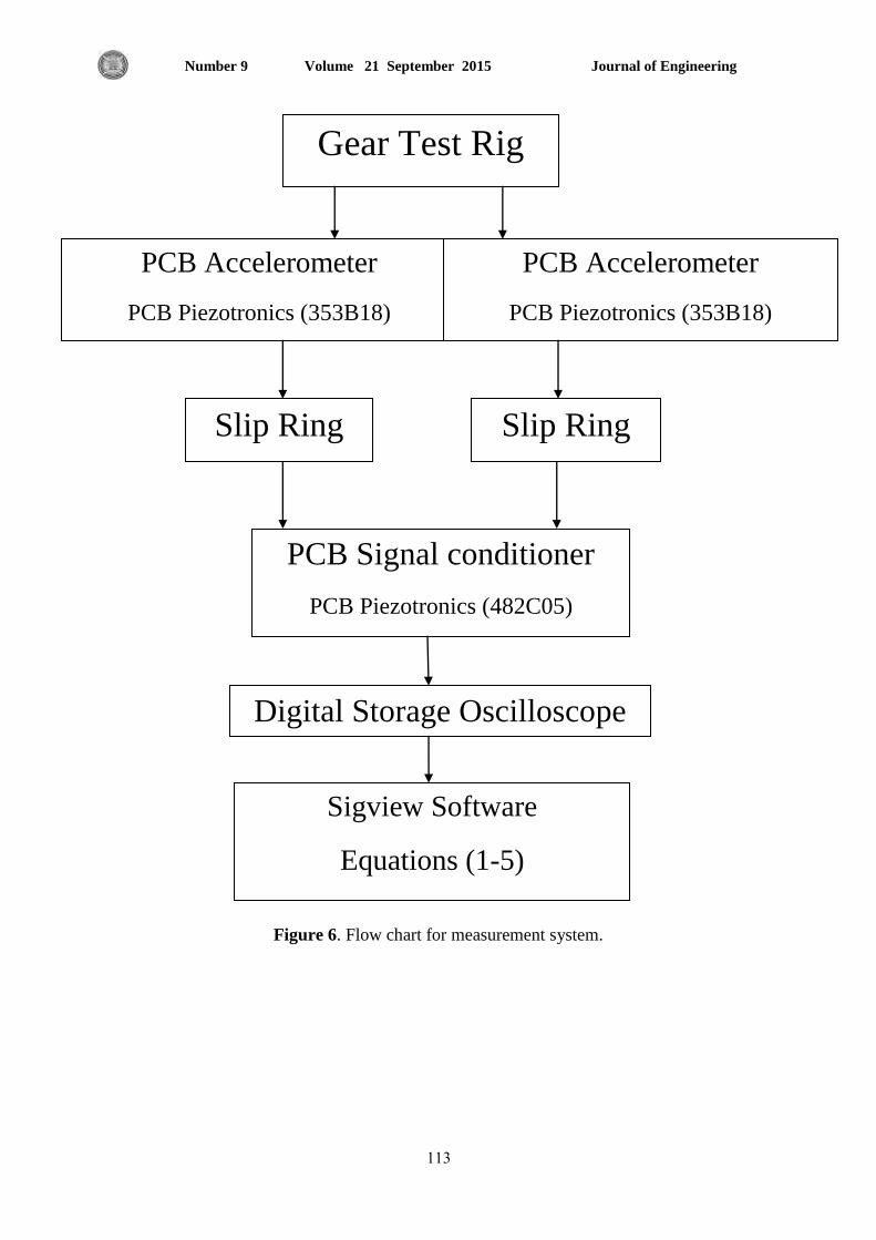
Journal of Engineering Volume 21 September 2015 Number 9
113
Figure 6. Flow chart for measurement system.
Gear Test Rig
Slip Ring
Slip Ring
PCB Accelerometer
PCB Piezotronics (353B18)
,,mmm
Mmnnbnn jbvl
PCB Signal conditioner
PCB Piezotronics (482C05)
Digital Storage Oscilloscope
PCB Accelerometer
PCB Piezotronics (353B18)
,,mmm
Mmnnbnn jbvl
Sigview Software
Equations (1-5)

Journal of Engineering Volume 21 September 2015 Number 9
114
Figure 7.The Variation of sound intensity level for asymmetric gear with and without tip relief.
Figure 8. Dynamic load factor for symmetric& asymmetric gears.
60
65
70
75
80
85
90
95
100
105
110
115
0 500 1000 1500 2000 2500 3000 3500 4000
sou
nd
leve
l (d
b)
Rotation (rpm)
Case (6)
Case (1)
0
1
2
3
4
5
6
7
8
0 500 1000 1500 2000 2500 3000
Dyn
amic
load
Fac
tor
Rotation (rpm)
symmetric Gear
asymmetric Gear
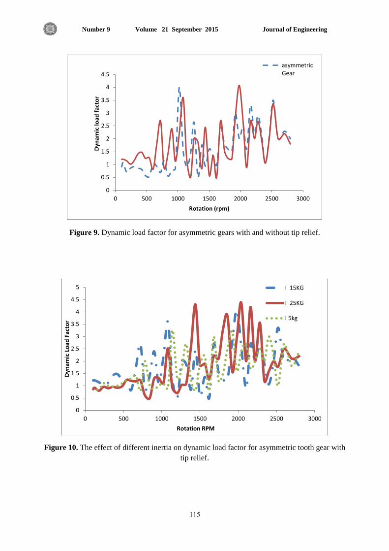
Journal of Engineering Volume 21 September 2015 Number 9
115
Figure 9. Dynamic load factor for asymmetric gears with and without tip relief.
Figure 10. The effect of different inertia on dynamic load factor for asymmetric tooth gear with
tip relief.
0
0.5
1
1.5
2
2.5
3
3.5
4
4.5
0 500 1000 1500 2000 2500 3000
Dyn
amic
load
fac
tor
Rotation (rpm)
asymmetricGear
0
0.5
1
1.5
2
2.5
3
3.5
4
4.5
5
0 500 1000 1500 2000 2500 3000
Dyn
amic
Lo
ad F
acto
r
Rotation RPM
I 15KG
I 25KG
I 5kg

Journal of Engineering Volume 21 September 2015 Number 9
116
Figure 11. Dynamic load factor for symmetric gear and asymmetric gear with tip relief and
loaded pressure angle (250).
Figure 12. Dynamic transmission error for symmetric and asymmetric gear.
0
1
2
3
4
5
6
7
8
0 500 1000 1500 2000 2500 3000
Dyn
amic
load
fac
tor
Rotaion(rpm)
Asymmetric gear withtip relief (ØL 25)
Symmetric gear
0
10
20
30
40
50
60
70
80
90
0 500 1000 1500 2000 2500 3000
Dya
nm
ic t
ran
smis
sio
n e
rro
r (m
icro
n)
Rotation (rpm)
Symmetric gear
AsymmetricGear
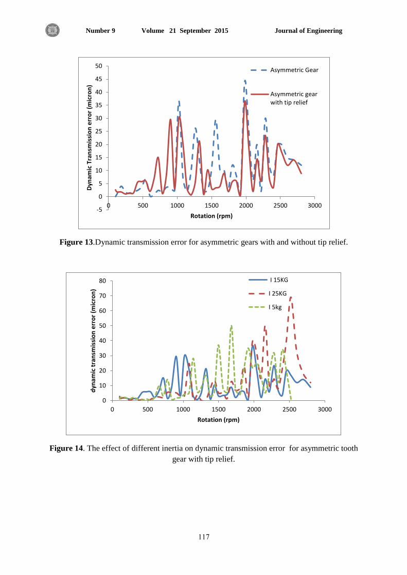
Journal of Engineering Volume 21 September 2015 Number 9
117
Figure 13.Dynamic transmission error for asymmetric gears with and without tip relief.
Figure 14. The effect of different inertia on dynamic transmission error for asymmetric tooth
gear with tip relief.
-5
0
5
10
15
20
25
30
35
40
45
50
0 500 1000 1500 2000 2500 3000
Dyn
amic
Tra
nsm
issi
on
err
or
(mic
ron
)
Rotation (rpm)
Asymmetric Gear
Asymmetric gearwith tip relief
0
10
20
30
40
50
60
70
80
0 500 1000 1500 2000 2500 3000
dyn
amic
tra
nsm
issi
on
err
or
(mic
ron
)
Rotation (rpm)
I 15KG
I 25KG
I 5kg

Journal of Engineering Volume 21 September 2015 Number 9
118
Table 1. Design parameters of symmetric, asymmetric and asymmetric with tip relief of spur gear
drive.
Gear parameter Symmetric gear
drive
(pinion and gear
)
Asymmetric gear
drive
(pinion and gear)
Asymmetric gear
drive with tip
relief
(pinion and gear )
Pressure angle 20 o /20
o 14.5
o /25
o 14.5
o /25
o
Module 7 mm 7 mm 7mm
Face width 60 mm 60 mm 60 mm
Teeth number 14 14 14
Tooth addendum
height
7 mm 7 mm 7 mm
Tooth dendum
height
8.16 mm 8.16 mm 8.16 mm
Fillet radius 2.1 mm 2.1 mm 2.1 mm
Relief amount - - 40 micron
Relief specification - - 0.33 pb
Table 2. Maximum dynamic load factor and maximum dynamic transmission error for different
gear types.
Gear type Maximum Dynamic load
Factor
Maximum Dynamic
Transmission Error
(micron)
Symmetric
6.1 75
Asymmetric
4 40
Asymmetric with tip
relief ( I 5kg)
3.2 45
Asymmetric with tip
relief ( I 15kg)
3.3 35
Asymmetric with tip
relief ( I 25kg)
4.2 65
Asymmetric with tip
relief ( I 35kg)
3.4 32

Journal of Engineering Volume 21 September 2015 Number 9
119
Internal Convective Heat Transfer Effect on Iraqi Building Construction
Cooling Load
Khalid Ahmed Joudi Ali Naser Hussien
Professor Lecturer
College of Engineering-University of Baghdad department of Mechanical engineering -University of
Technology
E-mail: [email protected] E-mail: [email protected]
ABSTRACT
This work involves the calculation of the cooling load in Iraqi building constructions taking in
account the effect of the convective heat transfer inside the buildings. ASHRAE assumptions are
compared with the Fisher and Pedersen model of estimation of internal convective heat transfer
coefficient when the high rate of ventilation from ceiling inlet configuration is used. Theoretical
calculation of cooling load using the Radiant Time Series Method (RTSM) is implemented on the
actual tested spaces. Also the theoretical calculated cooling loads are experimentally compared by
measuring the cooling load in these tested spaces. The comparison appears that using the modified
Fisher and Pedersen model when large ventilation rate is used; modify the results accuracy to
about 10%.
Key words: surface conductance, Iraqi building cooling load calculation.
لأبنت عراقت انتركب الإنشائ عهى حمم انتبرذبانحمم انذاخه تأثر انتقال انحرارة
عه ناصر حسن خانذ أحمذ جودي
يذسس أسرار
انجايؼح انركنجيح -قسى انذسح انيكايكيحجايؼح تغذاد -كهيح انذسح
انخلاصت
م داخم في ذشاكية انثاء انؼشاقي يغ الأخز في الاػرثاس ذأثيش ارقال انحشاسج تانححساب حم انرثشيذ انؼم انحاني يرض
يؼايم ارقال انحشاسج انذاخهي ػذ اسرخذاو يؼذلاخ ػانيح في ذخي تذسس فشضيح اششي قسد يغ طشيقح فيششانثايح.
( (RTSMتاسرخذاو طشيقح انسهسهح انزييح نلإشؼاع احرساب حم انرثشيذ ظشيا . ذى نحانح ذجيز اناء ي انسقف نهريح
انقاسح .فضاءاخان انرثشيذ في زتقياس حم ػهيا يقاسرذى فا حم انرثشيذ انحسب ظشيا . كزنكححقيقي اخرثاس نفضاءاخ
%.11انؼذنح نؼذلاخ كثيشج ي انريح, يحس دقح انرائج نحذد ذصم ل فيشش تذسسا اسرخذاو طشيقح أظشخ
.اقيحلأتيح ػش ياصهح انسطح, حساب حم انرثشيذ انرئسه: انكهماث

Journal of Engineering Volume 21 September 2015 Number 9
121
1. INTRODUCTION The nature of air motion in the air-conditioned space is one of the important features to provide a
uniform temperature, humidity, and velocity distributions to insure a comfort sense in this space.
In the other hand the air conditioning equipment energy cost as a result from the variation of heat
transfer by convection through the construction is influenced by the velocity and the configuration
of air movement in the space. Many efforts are made in this field to estimate the essential
parameters affect, to achieve the actual conception of the relation between the air movement and
heat transfer.
The internal heat transfer coefficient can be combined as the conductance in the inside of the
structure which is one component of overall heat transfer coefficient (U value). ASHRAE assumes
that the flow of internal air near walls and roofs by buoyancy only and sometimes called “still air”,
ASHRAE, 2009 and according to this assumption the values of the inside surface conductance hi
and the resistance Ri given by ASHRAE assuming natural convection heat transfer. These values
indicated in table 1 are satisfied for many cases of air-conditioning, but the new studies of
convective heat transfer in buildings, showed that for other cases, natural convection film
coefficients significantly underpredict the rate of surface convective heat transfer, especially at
high rate of air movement. Results of experimental convective heat transfer validation inside room
found from Ferguson, 1979, and investigation of forced convective heat transfer coefficient at
high flow rate of air ventilation introduced by Kooi and Forch 1985, both works appear that the
convective heat transfer coefficient is impacted by the volumetric air flow rate and the air inlet
temperature.
Experimental cooling load calculations for the room done by Spitler et al. 1987 showed that the
assumption of an adiabatic floor and free convection from ceiling in air conditioning spaces were
incorrect. Convection coefficients correlated with twenty-seven data point by multi regression as a
function of temperature difference between air and building interior surface was introduced by
Khalifa and Marshall 1990 and these coefficients are differ from ASHRAE data. Alamdari
1991 studied the thermo-fluid analysis of the building environment using CFD model. Effect of air
inlet location on the thermal comfort and inside air motion were analyzed by Vazques et al. 1991,
and found that the temperature and flow field are greatly related to the air inlet location. A
convective internal heat transfer correlations were experimentally investigated by Spitler et al.
1991 depending on the ventilation rate by momentum number of air inlet, the correlations include
roof, wall, and floor internal convective heat transfer coefficients and for wall grille air inlet.
The study of Fisher and Pedersen, 1997 was correlated the value of the internal convective
heat transfer coefficient for ceiling inlet configuration as a function of an enclosure air change rate
per hour (ACH) within the range (3 < ACH< 100). The correlations are indicated in table 2 for
roofs, walls and floors. Fisher and Pedersen concluded that the error resulted in cooling load using
ASHRAE assumption of hi under predict the actual measuring values by more than 10%.
Djuneady 2000, Djuneady et al. 2003; Djuneady et al. 2004; Djuneady et al. 2005 simulated
the air flow pattern in the air conditioned room using the coupling between the Building Energy
Simulation (BES) and Computational Fluid Dynamics (CFD) (Fluent) model compared with
experimental measurement; they concluded that the inlet conditions of the air have significant
effect on the flow pattern.
The summary of concepts can be concluded from the above works that, the inlet air temperature,
velocity, and configuration are greatly affected the indoor air movement and the convective heat
transfer in the air conditioned spaces and then the accuracy of cooling load estimation. Also the
adoption of ASHRAE model of Inside surface conductance hi and the resistances Ri given by
assumed natural convection heat transfer that illustrated in Table 1 are underestimate the cooling
load calculation in many cases of high rate air movement.

Journal of Engineering Volume 21 September 2015 Number 9
121
Therefore the suitable correlations such as Fisher and Pedersen correlations that relate the inside
surface heat transfer coefficient to the air change per hour (ACH) should be adopted in cooling
load calculation at high rate of ventilation, these correlations gave practical estimation to inside
surface heat transfer coefficient and easy to use for ceiling inlet configuration (air supply from
ceiling diffusers).
The objectives of the present work are:
1. Using Fisher and Pedersen correlation of internal convective heat transfer coefficient for
ceiling inlet configuration listed in Table 2 in calculating of cooling load for three air
conditioned spaces with high rate of ventilation.
2. Repeat cooling load calculation in 1 above for the same spaces but using ASHRAE
model of convective heat transfer coefficient illustrated in Table 1.
3. Using Radiant Time Series (RTS) method which is the latest ASHRAE method of
cooling load calculation in 1 and 2 above.
4. Compare the results in 1 and 2 above with the actual experimental measurement of
cooling load for the three test spaces mentioned in 1 above, to explore the accuracy of
these results.
2. CALCULATION PROCEDURES IN RTS METHOD
2.1 Heat Gain Calculations in RTS Method
Wall and roof conductive heat input at the exterior at n hours ago is defined by the familiar
conduction equation:
Qi,t-n = UA(Te,t-n – Ti) (1)
where Ti is the indoor temperature and Te,t-n is the sol-air temperature at n hours ago and is
expressed as:
(2)
Conductive heat gain through walls or roofs can be calculated using conductive heat inputs for
the current hour and past 23 hours and conduction time series , ASHRAE 2009.
Qt = cf0Qi,t + cf1Qi,t-1 + cf2Qi,t-2 + cf3Qi,t-3 + … + cf23Qi,t-23 (3)
cf0, cf1, etc. represent the conduction time factors. Multiplying of the conduction time factors by
the U value gives the periodic response factors, pr and Eq. (3) may be rewritten as:
( ) ( ) ( ) (4)
Periodic response factors, pr can be evaluated by using Periodic Response Factor / Radiant Time
Factor (PRF/RTF) Generator software published by Iu and Fisher in 2001. at Oklahoma state
university. The program yields the conduction transfer function coefficients, the periodic response
factors, and the U value, by giving the physical properties of any structure with any number of
layers. These physical properties include; thickness, thermal conductivity, density, and specific
heat for each layer of a homogeneous material constituting the wall or roof. For non-homogeneous
materials and for air gaps and air films in and outside the structure, the equivalent thermal
resistance is the input instead of other physical properties.
Journal of Engineering Volume 21 September 2015 Number 9
122
The heat gain from glass and the other components in the space can be calculated by reviewing
chapters 15 and 18 of ASHRAE Handbook of Fundamentals 2009.
2.2 Conversion of Heat Gain to Cooling Load
The heat gains of all components are divided into convective and radiative heat gain portions.
Table 14 in chapter 18 of ASHRAE Handbook of Fundamentals 2009 illustrates the
recommended radiative / convective splits for each component heat gain. The hourly convective
portion heat gain is directly converted to hourly convective cooling load, whereas the appropriate
radiant time series are applied to the hourly radiant portion heat gains to account for time delay in
conversion to cooling load.
The radiant time series or Radiant Time Factors (RTF) are the series of 24 factor denoted by r
in the present study and generated from heat balance procedures between interior surfaces radiant
heat gain and room air for different types of structures, fenestrations, and furnishing. These factors
are tabulated for specific cases, (as indicated in table 19 and 20 in chapter 18 of ASHRAE
Handbook of Fundamentals 2009) to use them directly for the certain application instead of
performing inside surface and room air heat balances. Converting the radiant portion of hourly
heat gains into hourly cooling loads is accomplished by the following equation ASHRAE 2009:
Qclr,t = r0Qr,t + r1Qr,t –1 + r2Qr,t –2 + r3Qr,t –3 + … + r23Qr,t –23 (5)
The hourly radiant portion cooling load calculated in Eq. (5) above is then added to the hourly
convective cooling load to obtain the total hourly cooling load for a certain component.
2.3 Inside Surface Heat Transfer Coefficient (hi) The convective heat transfer coefficients in Fisher and Pedersen correlations are based on a
reference temperature measured in the supply air duct, which are calculated from the rate of
convective heat transfer and the temperature difference between the interior surface temperature
and the supply air temperature as follows (Fisher and Pedersen 1997):
⁄ (6)
The use of supply temperature as the reference temperature provides larger temperature
differences between the surface and the air reference temperature, which enables the development
of more accurate exponents and convection correlations, as proposed by Spitler et al. , 1991a,
1991b).
Also the internal convective heat transfer coefficient can be calculated based on the room air
temperature as a reference temperature as follows ,Goldstein and Novoselac 2010.
⁄ (7)
The choice of reference temperature, as either room temperature (Ti) or air supply temperature
(Ts), is dependent upon the dominant mode of convection within the room. If natural convection
dominates, then room temperature is appropriate as a reference as long as the air is well mixed.
However, as room air can be stratified due to the effect of buoyancy when natural convection
dominates, the temperature must be taken at multiple points vertically from floor to ceiling, and
averaged for an accurate reading. Whereas the choice of air supply temperature (Ts) as a reference
temperature is more appropriate when forced convection dominates ,Goldstein and Novoselac
2010.
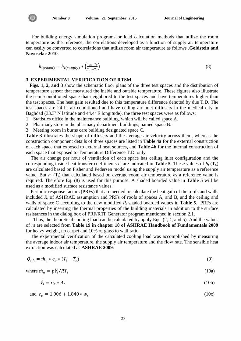
Journal of Engineering Volume 21 September 2015 Number 9
123
For building energy simulation programs or load calculation methods that utilize the room
temperature as the reference, the correlations developed as a function of supply air temperature
can easily be converted to correlations that utilize room air temperature as follows ,Goldstein and
Novoselac 2010.
(
) (8)
3. EXPERIMENTAL VERIFICATION OF RTSM
Figs. 1, 2, and 3 show the schematic floor plans of the three test spaces and the distribution of
temperature sensor that measured the inside and outside temperature. These figures also illustrate
the semi-conditioned space that neighbored to the test spaces and have temperatures higher than
the test spaces. The heat gain resulted due to this temperature difference denoted by due T.D. The
test spaces are 24 hr air-conditioned and have ceiling air inlet diffusers in the medical city in
Baghdad (33.3o N latitude and 44.4
o E longitude), the three test spaces were as follows:
1. Statistics office in the maintenance building, which will be called space A.
2. Pharmacy store in the pharmacy department buildings, named space B.
3. Meeting room in burns care building designated space C.
Table 3 illustrates the shape of diffusers and the average air velocity across them, whereas the
construction component details of three spaces are listed in Table 4a for the external construction
of each space that exposed to external heat sources, and Table 4b for the internal construction of
each space that exposed to Temperature Difference T.D. only.
The air change per hour of ventilation of each space has ceiling inlet configuration and the
corresponding inside heat transfer coefficients hi are indicated in Table 5. These values of hi (TS)
are calculated based on Fisher and Pedersen model using the supply air temperature as a reference
value. But hi (Ti) that calculated based on average room air temperature as a reference value is
required. Therefore Eq. (8) is used for this purpose. A shaded boarded value in Table 5 will be
used as a modified surface resistance values.
Periodic response factors (PRFs) that are needed to calculate the heat gain of the roofs and walls
included Ri of ASHRAE assumption and PRFs of roofs of spaces A, and B, and the ceiling and
walls of space C according to the new modified Ri shaded boarded values in Table 5. PRFs are
calculated by inserting the thermal properties of the building materials in addition to the surface
resistances in the dialog box of PRF/RTF Generator program mentioned in section 2.1.
Thus, the theoretical cooling load can be calculated by apply Eqs. (2, 4, and 5). And the values
of rs are selected from Table 19 in chapter 18 of ASHRAE Handbook of Fundamentals 2009
for heavy weight, no carpet and 10% of glass to wall ratio.
The experimental verification of the calculated cooling load was accomplished by measuring
the average indoor air temperature, the supply air temperature and the flow rate. The sensible heat
extraction was calculated as ASHRAE 2009:
(9)
where ⁄ (10a)
(10b)
and (10c)
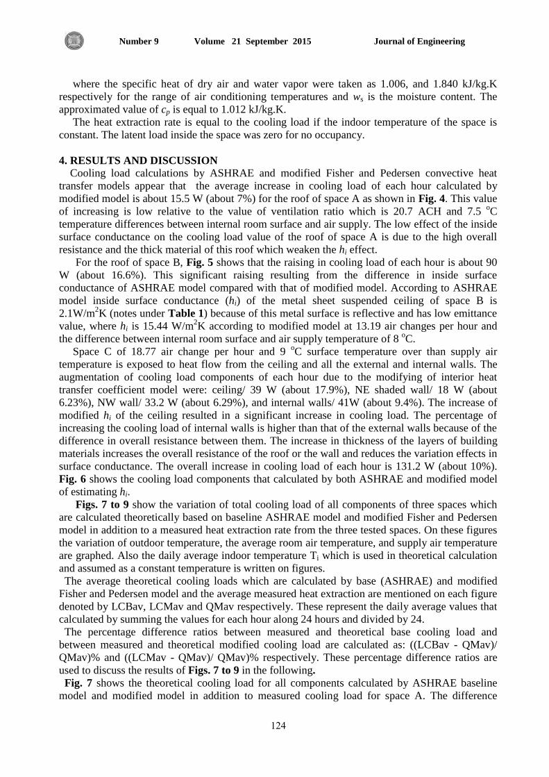
Journal of Engineering Volume 21 September 2015 Number 9
124
where the specific heat of dry air and water vapor were taken as 1.006, and 1.840 kJ/kg.K
respectively for the range of air conditioning temperatures and ws is the moisture content. The
approximated value of cp is equal to 1.012 kJ/kg.K.
The heat extraction rate is equal to the cooling load if the indoor temperature of the space is
constant. The latent load inside the space was zero for no occupancy.
4. RESULTS AND DISCUSSION
Cooling load calculations by ASHRAE and modified Fisher and Pedersen convective heat
transfer models appear that the average increase in cooling load of each hour calculated by
modified model is about 15.5 W (about 7%) for the roof of space A as shown in Fig. 4. This value
of increasing is low relative to the value of ventilation ratio which is 20.7 ACH and 7.5 oC
temperature differences between internal room surface and air supply. The low effect of the inside
surface conductance on the cooling load value of the roof of space A is due to the high overall
resistance and the thick material of this roof which weaken the hi effect.
For the roof of space B, Fig. 5 shows that the raising in cooling load of each hour is about 90
W (about 16.6%). This significant raising resulting from the difference in inside surface
conductance of ASHRAE model compared with that of modified model. According to ASHRAE
model inside surface conductance (hi) of the metal sheet suspended ceiling of space B is
2.1W/m2K (notes under Table 1) because of this metal surface is reflective and has low emittance
value, where hi is 15.44 W/m2K according to modified model at 13.19 air changes per hour and
the difference between internal room surface and air supply temperature of 8 oC.
Space C of 18.77 air change per hour and 9 oC surface temperature over than supply air
temperature is exposed to heat flow from the ceiling and all the external and internal walls. The
augmentation of cooling load components of each hour due to the modifying of interior heat
transfer coefficient model were: ceiling/ 39 W (about 17.9%), NE shaded wall/ 18 W (about
6.23%), NW wall/ 33.2 W (about 6.29%), and internal walls/ 41W (about 9.4%). The increase of
modified hi of the ceiling resulted in a significant increase in cooling load. The percentage of
increasing the cooling load of internal walls is higher than that of the external walls because of the
difference in overall resistance between them. The increase in thickness of the layers of building
materials increases the overall resistance of the roof or the wall and reduces the variation effects in
surface conductance. The overall increase in cooling load of each hour is 131.2 W (about 10%).
Fig. 6 shows the cooling load components that calculated by both ASHRAE and modified model
of estimating hi.
Figs. 7 to 9 show the variation of total cooling load of all components of three spaces which
are calculated theoretically based on baseline ASHRAE model and modified Fisher and Pedersen
model in addition to a measured heat extraction rate from the three tested spaces. On these figures
the variation of outdoor temperature, the average room air temperature, and supply air temperature
are graphed. Also the daily average indoor temperature Ti which is used in theoretical calculation
and assumed as a constant temperature is written on figures.
The average theoretical cooling loads which are calculated by base (ASHRAE) and modified
Fisher and Pedersen model and the average measured heat extraction are mentioned on each figure
denoted by LCBav, LCMav and QMav respectively. These represent the daily average values that
calculated by summing the values for each hour along 24 hours and divided by 24.
The percentage difference ratios between measured and theoretical base cooling load and
between measured and theoretical modified cooling load are calculated as: ((LCBav - QMav)/
QMav)% and ((LCMav - QMav)/ QMav)% respectively. These percentage difference ratios are
used to discuss the results of Figs. 7 to 9 in the following.
Fig. 7 shows the theoretical cooling load for all components calculated by ASHRAE baseline
model and modified model in addition to measured cooling load for space A. The difference
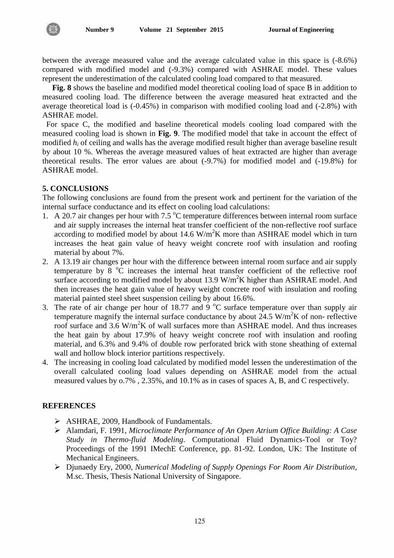
Journal of Engineering Volume 21 September 2015 Number 9
125
between the average measured value and the average calculated value in this space is (-8.6%)
compared with modified model and (-9.3%) compared with ASHRAE model. These values
represent the underestimation of the calculated cooling load compared to that measured.
Fig. 8 shows the baseline and modified model theoretical cooling load of space B in addition to
measured cooling load. The difference between the average measured heat extracted and the
average theoretical load is (-0.45%) in comparison with modified cooling load and (-2.8%) with
ASHRAE model.
For space C, the modified and baseline theoretical models cooling load compared with the
measured cooling load is shown in Fig. 9. The modified model that take in account the effect of
modified hi of ceiling and walls has the average modified result higher than average baseline result
by about 10 %. Whereas the average measured values of heat extracted are higher than average
theoretical results. The error values are about (-9.7%) for modified model and (-19.8%) for
ASHRAE model.
5. CONCLUSIONS The following conclusions are found from the present work and pertinent for the variation of the
internal surface conductance and its effect on cooling load calculations:
1. A 20.7 air changes per hour with 7.5 oC temperature differences between internal room surface
and air supply increases the internal heat transfer coefficient of the non-reflective roof surface
according to modified model by about 14.6 W/m2K more than ASHRAE model which in turn
increases the heat gain value of heavy weight concrete roof with insulation and roofing
material by about 7%.
2. A 13.19 air changes per hour with the difference between internal room surface and air supply
temperature by 8 oC increases the internal heat transfer coefficient of the reflective roof
surface according to modified model by about 13.9 W/m2K higher than ASHRAE model. And
then increases the heat gain value of heavy weight concrete roof with insulation and roofing
material painted steel sheet suspension ceiling by about 16.6%.
3. The rate of air change per hour of 18.77 and 9 oC surface temperature over than supply air
temperature magnify the internal surface conductance by about 24.5 W/m2K of non- reflective
roof surface and 3.6 W/m2K of wall surfaces more than ASHRAE model. And thus increases
the heat gain by about 17.9% of heavy weight concrete roof with insulation and roofing
material, and 6.3% and 9.4% of double row perforated brick with stone sheathing of external
wall and hollow block interior partitions respectively.
4. The increasing in cooling load calculated by modified model lessen the underestimation of the
overall calculated cooling load values depending on ASHRAE model from the actual
measured values by o.7% , 2.35%, and 10.1% as in cases of spaces A, B, and C respectively.
REFERENCES
ASHRAE, 2009, Handbook of Fundamentals.
Alamdari, F. 1991, Microclimate Performance of An Open Atrium Office Building: A Case
Study in Thermo-fluid Modeling. Computational Fluid Dynamics-Tool or Toy?
Proceedings of the 1991 IMechE Conference, pp. 81-92. London, UK: The Institute of
Mechanical Engineers.
Djunaedy Ery, 2000, Numerical Modeling of Supply Openings For Room Air Distribution,
M.sc. Thesis, Thesis National University of Singapore.

Journal of Engineering Volume 21 September 2015 Number 9
126
Djunaedy, E., Hensen, J.L.M., Loomans, M.G.L.C. 2003, Toward External Coupling of
Building Energy and Airflow Modeling Programs, ASHRAE Transactions, Vol. 109, No.
2, pp. 771-787.
Djunaedy, E., Hensen, J.L.M., Loomans, M.G.L.C. 2004. Comparing Internal and
External Run-Time Coupling of CFD And Building Energy Simulation Software, Proc.
Room vent 2004, Coimbra, Portugal.
Djunaedy, E., Hensen, J.L.M., Loomans, M.G.L.C. 2005, External Coupling Between CFD
and Energy Simulation: Implementation and Validation, ASHRAE Transactions, 111 (1),
pp. 612-624.
Fisher, D.E., and C.O. Pedersen. 1997. Convective Heat Transfer in Building Energy and
Thermal Load Calculations, ASHRAE Transactions, vol. 103, pt. 2, pp. 137-148.
Ferguson Jeffry Don, 1979, Experimental Convective Heat Transfer Facility, Testing and
Validation. M.sc. Thesis, Oklahoma State University.
Goldstein, K., and Novoselac, A., 2010 Convective Heat Transfer in Rooms with Ceiling
Slot Diffusers. www.ASHRAE.org
Iu Ip seng and Fisher D.E. ,2001.www.hvac.okstate.edu
Khalifa A.J.N. and Marshall R.H.,1990., Validation of Heat Transfer Coefficients on
Interior Building Surfaces Using a Real-Sized Indoor Test Cell, Int. J. Heat and Mass
Transfer, vol. 33 (10), pp. 2219-2236.
Kooi van der, J., and E. Forch. 1985. Calculation of the Cooling Load by Means of a
"More-Air-Points-Model." Proceedings of the CLIMA 2000 World Congress on Heating,
Ventilating and Air-Conditioning 4: 395-40l.
Spitler, J.D., C.O. Pedersen, and R.J. Bunkofske. 1987, Experimental Study of Interior
Convective and Radiative Heat Transfer in Buildings. Heat Transfer in Buildings and
Structures, ASME HTD, Vol. 78, pp. 67- 76. New York: American Society of Mechanical
Engineers
Spitler, J., C. Pedersen, D. Fisher, P. Menne, and J. Cantillo. 1991a. Design of an
Experimental Facility For Investigation of Interior Convective Heat Transfer Under
Ventilative Cooling Conditions. ASHRAE Transactions 97(1).
Spitler, J., C. Pedersen, and D. Fisher. 1991b. Interior Convective Heat Transfer in
Buildings with Large Ventilative Flow Rates. ASHRAE Transactions 97(1).
Vazquez, B., Samano, M., and Yianneskis, M. (1991), The Effect of Air Inlet Location on
the Ventilation of an Auditorium. Computational Fluid Dynamic-Tool orToy? Proceedings
of the 1991 IMechE Conference, pp. 56-66. London, UK: The Institute of Mechanical
Engineers.
NOMENCLATURE
A area m2
cp specific heat of air kJ/kgK
cf conduction time factor
hi, ho inside, outside heat transfer coefficient W/m2K
I solar radiation W/m2
m∙a air mass flow rate kg/s
p atmospheric pressure pa
pr periodic response factor W/m2K
Q heat W
R gas constant of air kJ/kgK
Ri internal surface thermal resistance m2K/W

Journal of Engineering Volume 21 September 2015 Number 9
127
∆R the difference between the long wave radiation incident on the surface from the sky and
surroundings, and the radiation emitted by a black body at the outdoor air temperature W/m2
r radiant time factor
T temperature °C
t time sec
U overall heat transfer coefficient W/m2K
air supply velocity m/s
V˙s air supply volume flow rate m3/s
ws moisture content kgwater/kgair
Greek Symbols
e emittance of the surface
m absorptivity of the surface
Subscripts
a air
c cross sectional (diffuser area)
e sol-air (Temperature)
i indoor
o outdoor
s supply
t total (solar radiation), time (others)
Abbreviations
ACH Air Change per Hour
due T.D due temperature difference
LCBav average Calculated Baseline Load W
LCMav average Calculated Modified Load W
PRF Periodic Response Factor W/m2K
QMav average Measured Load W
RTS Radiant Time Series
RTSM Radiant Time Series Method
tot. calc.base total cooling load calculated according to base (ASHRAE) model W
tot. calc.Mod. total cooling load calculated according to modified model W
Table 1. Surface conductances and resistances for air, ASHRAE 2009.
* Surface emittance of ordinary building materials is 0.9 and for metals and metal paint between
0.05 and 0.5
Position of
surface (assume
still air)
Direction
of
heat flow
Nonreflective surfaces Reflective surfaces
Emittance,* ε= 0.90 Emittance,ε=0.20 Emittance,ε=0.05
hi
W/m2K
Ri m
2K/W
hi
W/m2K
Ri m
2K/W
hi
W/m2K
Ri m
2K/W
Horizontal
Sloping at 45°
Vertical
Sloping at 45°
Horizontal
Upward
Upward
Horizontal
Downward
Downward
9.26
9.09
8.29
7.50
6.13
0.11
0.11
0.12
0.13
0.16
5.17
5.00
4.20
3.41
2.10
0.19
0.20
0.24
0.29
0.48
4.32
4.15
3.35
2.56
1.25
0.2
0.24
0.30
0.39
0.80

Journal of Engineering Volume 21 September 2015 Number 9
128
Table 2. Heat transfer coefficients for ceiling inlet configuration (air supply from ceiling diffuser)
,Fisher and Pedersen 1997.
Surface type Correlation
Walls h= 0.19*ACH^0.8 (W/m2K)
Floor h= 0.13*ACH^0.8 (W/m2K)
Ceiling h= 0.49*ACH^0.8 (W/m2K)
Table 3. Diffuser shapes, dimensions, and air flow measuring data.
Space A B C
Average velocity m/s 6 7.133 1
Diffuser shapes
Table 4a. External wall, roof and floor construction details of tested spaces.
Spaces Constructions (from outside to inside) Direction
and area m2
A
Wall External air conductance +3 cm of cement plaster +30 cm thermo-stone
+1.5cm juss plaster +1 cm gypsum plaster + internal air conductance
NE=8.32
NW=15.05
Roof
External air conductance +4 cm of cement shtyger +5 cm of sand +1cm of
felt and membrane +5 cm of sty-rubber + 15 cm of high density concrete
+ air gap +acoustic tiles in suspended ceiling + internal air conductance
22.25
B
Wall External air conductance +2.5 cm of cement plaster +20 cm hollow block
+1.5cm juss plaster +1 cm gypsum plaster + internal air conductance
SW=34.65
SE=18
Roof
External air conductance +4 cm of cement shtyger +5 cm of sand +1cm of
felt and membrane +5 cm of sty-rubber + 20 cm of high density concrete
+ air gap + metal plates in suspended ceiling + internal air conductance
51
C Wall
External air conductance +5 cm of helan stone+ 5 cm of cement mortor
+24 cm perforated brick +1.5cm juss plaster +1 cm gypsum plaster +
internal air conductance
SW=17.2
SE=14.74

Journal of Engineering Volume 21 September 2015 Number 9
129
Table 4b. Internal wall, roof and floor construction details of tested spaces.
Spaces Constructions (from outside to inside) Area m2
A
Wall
Internal air conductance +1 cm gypsum plaster +1.5cm juss plaster +20 cm
hollow block +1.5cm juss plaster +1 cm gypsum plaster + internal air
conductance
7.92
floor Internal air conductance +20 cm of high density concrete+3cm cement
mortar+2.5cm mozaek tile +internal air conductance 22.25
B Wall Internal air conductance +2mm of steel sheet +air gap+ 2mm of steel sheet +
internal air conductance 40.635
C
walls
Internal air conductance +1 cm gypsum plaster +1.5cm juss plaster +20 cm
hollow block +1.5cm juss plaster +1 cm gypsum plaster + internal air
conductance
20.87
ceiling
Internal air conductance +2.5cm granite tile+3cm cement mortar +30 cm of
high density concrete+ air gap +1.5cm suspended ceiling +internal air
conductance
17.76
door Internal air conductance+5cm wood+ Internal air conductance 1.7
Table 5. Interior conductance according to Fisher and Pedersen model for the tested spaces.
spaces ACH Ts oC
Ti oC
Surface Tsi oC
hi(Ts)
W/m2K
hi(Ti)
W/m2K
Ri(Ti)
m2K/W
A 20.7 17 22.5
Ceiling 24.5 5.53 20.74 0.048
Walls 24.5 2.145 8 0.12
floor 24 1.47 6.86 0.146
B 13.19 17 23
Ceiling 25 3.86 15.44 0.065
Walls 25 1.5 6 0.16
floor 24 1.023 7.16 0.14
C 18.77 15.5 23
Ceiling 24.5 5.12 30.7 0.0325
Walls 24.5 1.98 11.88 0.084
floor 23.5 1.36 21.76 0.046

Journal of Engineering Volume 21 September 2015 Number 9
131
Figure 1. Schematic floor plan of tested space A.
Figure 2. Schematic floor plan of space B .
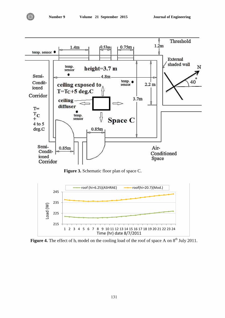
Journal of Engineering Volume 21 September 2015 Number 9
131
Figure 3. Schematic floor plan of space C.
Figure 4. The effect of hi model on the cooling load of the roof of space A on 8
th July 2011.
215
225
235
245
1 2 3 4 5 6 7 8 9 10 11 12 13 14 15 16 17 18 19 20 21 22 23 24
Load
(W
)
Time (hr) date 8/7/2011
roof (hi=6.25)(ASHRAE) roof(hi=20.7)(Mod.)

Journal of Engineering Volume 21 September 2015 Number 9
132
Figure 5. The effect of hi model on the cooling load of roof of space B on 25
th July 2011.
Figure 6. The effect of hi model on the cooling load of the ceiling and walls of space C on 15
th
July 2011.
500
520
540
560
580
600
1 2 3 4 5 6 7 8 9 10 11 12 13 14 15 16 17 18 19 20 21 22 23 24
Load
(W
)
Time (hr) date 25/7/2011
roof (hi=2.1)(ASHRAE) roof (hi=15.44)(Mod.)
140
190
240
290
340
390
440
490
540
590
1 2 3 4 5 6 7 8 9 10 11 12 13 14 15 16 17 18 19 20 21 22 23 24
Load
(W
)
Time (hr) date 15/7/2011
wall NE (shaded) hi=8.29(ASHRAE) wall NE (shaded) hi=11.88(Mod.)
wall NW hi=8.29(ASHRAE) wall NW hi=11.88(Mod.)
ceiling due T.D hi=6.3(ASHRAE) ceiling due T.D hi=30.7(Mod.)
interior walls due T.D.hi=8.29(ASHRAE) interior walls due T.D.hi=11.88(Mod.)

Journal of Engineering Volume 21 September 2015 Number 9
133
Figure 7. Cooling load comparison for the calculated baseline and modified model with the
measured load of space A on 8th
July 2011.
Figure 8. Cooling load comparison for the calculated base and modified model with the measured
load of space B on 25th
July 2011.
15
20
25
30
35
40
45
50
55
60
65
0
500
1000
1500
2000
2500
1 2 3 4 5 6 7 8 9 10 11 12 13 14 15 16 17 18 19 20 21 22 23 24
Ou
tdo
or
Tem
p. (
deg
.C)
Load
(W
)
Time (hr) date 8/7/2011
tot.calc.base tot.calc.Mod Qmeasured
Tout Tsupply TroomAve
Daily average
Ti=23.108 deg. C
LCBav=1836W LCMav=1850W QMav=2028.5W
13
23
33
43
53
63
800
1300
1800
2300
2800
3300
3800
4300
4800
1 2 3 4 5 6 7 8 9 10 11 12 13 14 15 16 17 18 19 20 21 22 23 24
Ou
tdo
or
Tem
p. (
deg
. C)
Load
(W
)
Time (hr) date 25/7/2011
tot.calc. base tot.calc. Mod Qmeasur.
Tout TaveRoom Tsupply
Daily average Ti=22.3 deg. C
LCBav=3501W LCMav=3586.5W QMav=3602.9W
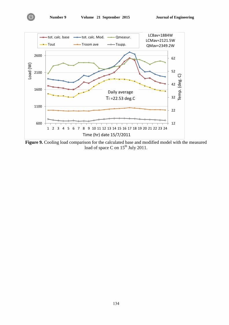
Journal of Engineering Volume 21 September 2015 Number 9
134
Figure 9. Cooling load comparison for the calculated base and modified model with the measured
load of space C on 15th
July 2011.
12
22
32
42
52
62
600
1100
1600
2100
2600
1 2 3 4 5 6 7 8 9 10 11 12 13 14 15 16 17 18 19 20 21 22 23 24
Tem
p. (
deg
. C)
Load
(W
)
Time (hr) date 15/7/2011
tot. calc. base tot. calc. Mod. Qmeasur.
Tout Troom ave Tsupp.
Daily average
Ti =22.53 deg.C
LCBav=1884W LCMav=2121.5W QMav=2349.2W

Journal of Engineering Volume 21 September 2015 Number 9
85
Mixed Convection Heat Transfer in a Vertical Saturated Concentric Annulus
Packed with a Metallic Porous Media
Dr. Mohammed A. Nima
Lecturer
Mechanical Engineering Department
College of Engineering- Baghdad University
E-mail: [email protected]
Sarmad A. Abdal Hussein Saud S.Hameed
Asst. Lecturer Mechanical Engineering Department
Mechanical Engineering Department Engineering College - Baghdad University
Engineering College - Baghdad University E-mail: [email protected]
E-mail: [email protected]
ABSTRACT
Mixed convection heat transfer in a vertical concentric annulus packed with a metallic porous
media and heated at a constant heat flux is experimentally investigated with water as the working
fluid. A series of experiments have been carried out with a Rayleigh number range from
Ra=122418.92 to 372579.31 and Reynolds number that based on the particles diameter of
Red=14.62, 19.48 and 24.36. Under steady state condition, the measured data were collected and
analyzed. Results show that the wall surface temperatures are affected by the imposed heat flux
variation and Reynolds number variation. The variation of the local heat transfer coefficient and the
mean Nusselt number are presented and analyzed. An empirical correlation has been proposed for
computing the Nusselt number for the geometry and boundary conditions under investigation.
Key words: mixed convection, concentric annulus, metallic porous media, constant heat flux.
اوتقال انحرارة بانحمم انمختهط في تجويف حهقي عمودي مشبع رو أسطواوتيه متمركزتيه تم حشوه بوسط
مسامي معذوي
انمذرس انذكتور محمذ عبذ انرؤوف وعمت
قسى انينذست انكانكت
جايعت بغذاد –كهت انينذست
سعود سويذان حميذ انمذرس انمساعذ سرمذ عزيز عبذ انحسيه
قسى انينذست انكانكت قسى انينذست انكانكت
جايعت بغذاد –كهت انينذست جايعت بغذاد –كهت انينذست
انخلاصت
قذ حى دساسخو انخقال انذشاسة بانذم انخخهط ف حجف دهق عد ر أسطانخن يخشكزحن حى دشه بسط يساي يعذن
ان 122418.92 ين سقى سانشاء عذد ين انخجاسب انعهت نذ . حى اجاسخخذاو اناء كائع يشغميع عهتبصسة
عنذ صل دانت الاسخقشاس حى جع . 16.44 24.61 ,26.41يذ سقى سننذ عه اساس قطش انجساث 372579.31
يعايم اظيشث اننخائج حأثش دسجاث دشاسة انسطخ حخأثش بخغش انفض انذشاس انسهط حغش سقى سننذ. حغش انباناث حذههيا.
يخسط سقى نسهج قذ حى اظياسىا دساسخيا. حى اقخشاح يعادنت حجشبت نذساب سقى نسهج نهشكم انز حى انضع انخقال انذشاسة
دساسخو يع انظشف انذذت انذطو بو.

Journal of Engineering Volume 21 September 2015 Number 9
86
فع دشاس ثابج. ، سط يساي يعذن،أسطانخن يخشكزحن، انذم انخخهطانكهماث انمفتاحيت:
1. INTRODUCTION
Heat transfer in porous media received great interest for many years because of the improved in
the heat transfer performance without proportionate increase in hydraulic resistance. It is well
known that the porous structure reduces the thickness of the boundary layer, increases the surface
area that in contact with the fluid and intensifies the mixing of the flowing fluid, and thus enhances
the thermal heat transfer. Flow and heat transfer through channels packed with porous media are
widely studied because of their potential applications in thermal management such as compact heat
electronic exchanges, solar collector, nuclear reactor cooling and regenerators. Packed bed has been
developed for different types of porous materials with specific intent to enhance the heat transfer
from the thermally loaded surfaces. Because of the random structures of porous media, they will be
different in engineering, physical and thermal properties, Venugopal, et al., 2010. As a result, flow
and heat transfer characteristics in these media also greatly differ. Renken and Poulikakos, 1990
investigated experimentally and numerically the forced convection heat transfer in the packed bed
areas of an occupied parallel plate channel whose walls maintain a constant temperature. Based on
this study, porous media needs to be considered as a viable alternative for the transfer of heat
enlarge in forced convection heat transfer in channels. Pu, et al., 1999, used R-113 loop in
performing the experiments of mixed convection heat transfer in a vertical packed channel with
asymmetric heating of opposing walls. Chrome steel beads of 6.35 mm in diameter were used as a
porous media. The experiments were carried out in the range of 2<Pe<2200 and 700<Ra<1500. The
measured temperature distribution indicated the existence of a secondary convective cell inside the
vertical packed channel in the mixed convection regime. A correlation equation for Nusselt number
in terms of Peclet number Pe and Rayleigh number Ra was obtained from experimental data. They
found that the following three convection regimes exist: natural convection regime: 105< Ra/Pe,
mixed convection regime: 1<Ra/Pe<105, and forced convection regime: Ra/Pe< 1. Dirker, 2000 presented a comparison of the literature that involving heat transfer in the ring. Their comparison
showed that there was a need for more research in the field of links convection heat transfer in
concentric ring as they found a little agreement among the existing relationship. Empirical
relationship for predicted Nusselt number in the ring had been developed with water as the working
fluid. Boomsma and Poulikakos, 2002 showed the results of experimental studies performance to
assess the hydraulic characteristics of open cell aluminum foam of different pore diameters and pore
in each of the compressed and non-compressed format. The study was done mainly to predict
important parameters permeability coefficient foam, precisely in order to describe the pressure drop
versus the flow behavior in the porous media. Hussein, et al., 2009 experimentally and theoretically
studied the convective heat transfer in vertical concentric annulus where the two cylinders filled
with porous medium. They concluded that the behavior of temperature profile were the same for any
diameters ratio and any different heat flux. The relation between Nu and Ra was proposed and the
results showed good agreement between experimental and theoretical studies. The potential of a

Journal of Engineering Volume 21 September 2015 Number 9
87
simple and inexpensive porous insert was experimentally investigated by Venugopal, et al., 2010.
The porous inserted consists of a stack of metallic perforated plates that used to enhance the heat
transfer from the heated wall of a vertical rectangular duct under forced flow conditions. The
characteristic features of the porous medium model on the hydrodynamic and heat transfer behavior
were investigated. The key novelty in this work was the development of a new correlation for the
Nusselt number that did not require any information from hydrodynamic studies. The largest
increase in the average Nusselt number of 4.52 times that for clear flow was observed with a porous
material of porosity of 0.85. Andrea, et al., 2012, investigated experimentally the air forced
convection through electrically heated open-cells copper foams with different number of pores per
unit of length (PPI) with constant porosity (ε=0.93) and foam core height of 40 mm. The
experimental heat transfer coefficient and pressure drop measurements permitted to understand the
effects of the pore density on the heat transfer and fluid flow performance of the foams. They
compared different enhanced surfaces, which can be considered suitable for electronic thermal
management against present author’s experimental measurements for 40 mm high aluminum foams
at the same operative test conditions.
To the best of the authors' knowledge, there is no existing experimental study on the mixed
convection heat transfer in a saturated concentric annulus that filled with metallic porous media. So
we proposed the present study to cover this shortage in the understanding of the flow and heat
transfer in porous enclosure with mixed convection effects.
In the present work, mixed convection heat transfer in a vertical saturated concentric porous
annulus subjected to a constant heat flux, is examined experimentally with water as the working
fluid. The main objective is to study the influence of mixed convection heat transfer on the flow
field and the associated heat transfer process in such system. The influence of heat flux and mass
flux variation on wall temperatures and Nusselt number are investigated and analysed then a general
relation that describe the overall process is presented.
2. EXPERIMENTAL APPARATUS AND PROCEDURE
2.1 Experimental Apparatus
The experimental investigation is carried out in an apparatus shown in Figs. 1 and 3. The
apparatus has been constructed to achieve the requirements of the present study and it consists of the
following major assemblies:
1- Test section
As shown in Fig. 2, the test section consists of two stainless steel cylinders that form a concentric
annulus of length L=63 cm. The inside and outside diameters of inner cylinder are
(Di=40 mm, Do=41mm) and the inside and outside diameters of outer cylinder are (Di=80 mm,
Do=82 mm). The inner and the outer cylinders are assembling together by means of two Teflon
flanges to form the concentric annulus test section. The Teflon flanges is used to reduce the
dissipative heat transfer from the test section ends and to support the inner and outer cylinders in one
concentric annulus by pushing them between the Teflon flanges inner and outer diameters (Di=39
mm, Do=83 mm). The wall thickness of each Teflon flange is 1.5 cm. Four holes are drilled in each

Journal of Engineering Volume 21 September 2015 Number 9
88
Teflon flange as shown in Fig. 2 but with different purposes. The holes in the lower flange are used
to distribute the incoming water from the liquid splitter and guide it uniformly to inter the test
section, while the holes in the upper flange are used as an exit passage for the thermocouples
extension wires that used to measure inner cylinder wall temperatures. The upper flange holes are
filled with a relatively high temperature adhesive material to support the thermocouples extension
wires and to prevent water infiltration. The concentric annulus is packed with stainless steel beads,
essentially spherical in shape with an average particles diameters of dp=6 mm. A metallic O-Ring
with holes (less than 6mm in diameter) is used to support the metallic porous media 13.5 cm far
from the test section lower end and to form an entrance length to achieve a uniform inlet water
velocity profile to the porous packing. The length of the porous packing was designed to be 40 cm
as shown in Fig. 2, and the water was then derived out of the test section by a tube that mounted at
9.5 cm far from the test section upper end. A uniform heat flux is provided on the outer surface of
the concentric annulus by a nickel-chrome wire of 1 mm in diameter, which is electrically insulated
and warps around the outer surface of the concentric annulus along the test section part that filled
with the metallic porous media (40 cm). This steel wire is supplied with AC-current from a voltage
regulator, to control the incoming current according to the heat flux desired. The test section is well
insulated outside with asbestos and fiber glass wool layers of 15 mm and 50 mm thickness,
respectively. The concentric annulus outer surface and inner surface temperatures are measured by
(18 K-type) thermocouples, which were distributed equally within nine sections along the outer
surface and inner surface of the concentric annulus as shown in Fig. 2. Another (5 K –type)
thermocouples were used to measure the water bulk temperature distribution by inserting these
thermocouples inside the test section through holes on the outer surface of the concentric annulus as
shown in Fig. 2. These holes are filled with a relatively high temperature adhesive material to
support the thermocouples extension wires and to prevent water infiltration. The temperature
distribution on the outer surface of the insulation shield are measured using (4 K-type)
thermocouples distributed in an equal pitch, to calculate the heat lost during the experiment by
referring to the temperature difference between the heater wall and the ambient. The heat lost is
found to be approximately 6% during the whole range of the imposed heat flux. A digital electronic
thermometer (type IDC-420042), is connected in parallel to the thermocouples by leads through a
selector switches, to record the temperature measurements.
2- Water supply
As shown in Fig. 1, the liquid supply assembly consists of water tank, valve, filter, flowmeter
(0.8 LPM full range) and liquid splitter, which are placed adjacent to the test section. A drain
reservoir was placed at the test section exit to collect the water. When the water exit from the test
section, it was forced to flow through a flexible tube that raise the water to a higher elevation (∆H)
before it collected in the drain reservoir. The purpose of this arrangement at the test section exit is to
control the test section pressure and to ensure that the water pressure inside the test section is higher
than the atmospheric pressure.
3- Electrical power measurement
The constant heat flux is supplied by using electrical circuit of alternating current that includes:
A) Voltage regulator.
B) Transformer.
C) Voltmeter.
D) Ammeter.

Journal of Engineering Volume 21 September 2015 Number 9
89
2.2 Experimental Procedure
Before starting the experimental measurements and in order to degas the air from the packed
annulus, the valve is opened in such a manner that the water flow at the flowmeter full range (0.8
LPM) and a moderate heat flux is applied for two to three hours. Then, the valve is adjusted to give
the required water flow rate. Each experiment is performed using the following procedure:
1) The valve that connected to the water tank is adjusted to give the required water flow rate
which is measured by the flowmeter.
2) The electrical power is switched on, and the heater input voltage is adjusted by a voltage
regulator to give the required voltage and current.
3) The supplied voltage and current to the heater are recorded to calculate the required
electrical power in accordance to the heat flux required.
4) The apparatus is left for two to three hours to establish the steady state condition. The
thermocouples readings are collected every half an hour. When the difference between two
readings became almost constant, the steady state condition is fixed and a final reading is
recorded.
To obtain a new set of experiments under the same water flow rate, a new electrical power is
selected, and the procedure from step 2 to 4 is repeated.
The net heat flux to the saturated porous media is determined from recording the electrical power
supplied to the heater and applying the following equation:
⁄ (1)
where;
Po= electrical power consumed by heater = I×V.
I = current flow through the heater.
V = voltage across the heater.
= surface area of the annulus outer cylinder.
Heat losses from the heater across asbestos and fiber glass wool layers are calculated to be 6%
while the heat losses from the axial direction through the Teflon flanges are found to be small and
neglected. These losses are subtracted from the electric power to obtain the net heat transfer rate.
3. HEAT TRANSFER CALCULATIONS
It is important to calculate the absolute permeability ( ), the effective thermal conductivity
( ) and the porosity ( ) of the saturated porous media, as they are used in the dimensionless
groups that govern the fluid flow and heat transfer calculations.
According to Nield and Bejan, 2006:
( ) (2)
( ) (3)

Journal of Engineering Volume 21 September 2015 Number 9
90
where and are the thermal conductivities of the water and the solid porous media, respectively.
The porosity of the packed stainless steel beads is found experimentally using the expression, Nield
and Bejan, 2006:
(4)
3.1 Reynolds Number
The Reynolds number can be defined according to the particle diameter and the fluid velocity at
the inlet as:
(5)
3.2 Grashof and Rayleigh Number
The Grashof number can be defined as:
(6)
then Rayleigh number (Ra) can be calculated using the following equation:
(7)
3.3 Local and mean Nusselt Number
The local heat transfer coefficient at the heated wall can be defined as:
(8)
Hence, the local and the mean Nusselt number can be calculated as, Nield and Bejan, 2006 :
( ) (9)
∫
(10)
The thermophysical properties of the water-stainless steel beads that used in the present study are
listed in Table 1 and the physical parameters for the stainless steel beads are listed in Table 2.
4. RESULTS AND DISCUSSION
A series of experiments have been carried out with a heat flux range from qw = 3912 W/m2 to
11907 W/m2
(Ra=122418.92 to 372579.31) and volumetric flow rate of Q = 0.3, 0.4 and 0.5 L/min
(Red=14.62, 19.48 and 24.36). The temperature distribution along the inner and the outer annulus
surfaces is measured and presented. The influence of heat flux variation and Reynolds number
variation on the local and mean heat transfer coefficient is discussed and analyzed. Finally, a general
correlation for the mean Nusselt number as a function of the parameters (Ra/Re) is derived to
describe the overall fluid flow and heat transfer behavior in the porous annulus.
Journal of Engineering Volume 21 September 2015 Number 9
91
4.1 The Influence of Heat Flux and Reynolds Number on the Surface Temperature
Distribution.
Figs. 4-6 show the influence of the imposed heat flux variation on the distribution of the outer
annulus surface temperature for Red=14.62, 19.48 and 24.36, respectively. A general trend can be
seen from Figs. 4-6, that the outer annulus surface temperature increases as the heat flux is increased
for the same Reynolds number value. When the imposed heat flux is increased (with a constant
Reynolds number), the buoyancy effect increases and causes a faster growth in the thermal boundary
layer along the porous annulus surface that will be associated with an increased in the outer annulus
surface temperature values.
Figs. 7-9 show the influence of the imposed heat flux variation on the distribution of the
temperature difference between the outer and the inner annulus surface temperature
[∆Tw=Tw, outer annulus surface − Tw, inner annulus surface] for Red=14.62, 19.48 and 24.36, respectively.
Figs. 7-9 show that the temperature difference (∆Tw) increases as the imposed heat flux is increased
for the same Reynolds number. It is clear from Fig. 7, that for a low Reynolds number (Red=14.62)
the fluctuation in the temperature difference (∆Tw) values with the axial distance is mild except for
qw = 11907 W/m2. When the heat flux is supplied on the outer annulus surface, the buoyance force
will caused an induced mass flux that will oppose the incoming cold-fluid and drive the hot fluid
from the vicinity of the outer heated wall towards the inner insulated wall and rising its temperature.
For low Reynolds number values, the buoyance effect increases and results in a faster heat transfer
from the outer to the inner annulus surface and as a consequence a smaller temperature difference
(∆Tw) as shown in Fig. 7.
While for a higher Reynolds numbers of Red=19.48 and 24.36 Figs. 8 and 9, the temperature
difference (∆Tw) increases with the axial distance and reaches its maximum value at Z=0.2 m from
the annulus entrance section and then it decreases downstream up to the annulus exit section. This
behavior can be explained based on the interaction between the buoyancy force and the inertia force
of the incoming cold-fluid. In the annulus entrance region the buoyancy force is still limited in
comparison with the inertia force of the incoming cold-fluid, and this will caused a retreat in the
thermal boundary layer growth from the outer annulus surface towards the inner annulus surface.
The domination of the incoming cold-fluid effect in the entrance region will cause a faster
temperature rise in the outer annulus surface and continues increased in the temperature difference
(∆Tw) with the axial distance to a point located at Z=0.2 m from the annulus entrance section as
shown in Figs. 8 and 9. In the region downstream of Z=0.2 m, the buoyancy force becomes stronger
due to the continuous heating and it will be able to overcome the inertia force of the incoming cold-
fluid. This will result in mobilizing more hot fluid from the vicinity of the outer heated wall towards
the inner insulated wall to rise its temperature and consequently we observe a remarkable decreased
in the temperature difference (∆Tw) as shown in Figs. 8 and 9. Another observation is made from
Figs. 7-9, that for higher Reynolds numbers (Red=19.48 and 24.36) the temperature difference (∆Tw)
increases suddenly at the annulus exit section. This can be attributed to the higher fluid mixing at the
annulus exit section as the hot fluid try to find its way out through the drain tube and this caused a

Journal of Engineering Volume 21 September 2015 Number 9
92
reduction in the inner annulus surface temperature and an increased in the temperature difference
(∆Tw) at the annulus exit.
Figs. 10-14 show the influence of Reynolds number variation on the distribution of the outer
annulus surface temperature for qw = 3912 W/m2 to 11907 W/m
2. The figures show that the surface
temperature decreases as the Reynolds number increased for the same heat flux value. When the
Reynolds number increased the thermal boundary layer retreat along the heated wall and as a
consequence a higher heat transfer rate can be expected that associated with a decrease in the outer
annulus surface temperature.
Figs. 15-19 show the influence of Reynolds number variation on the distribution of the
temperature difference between the outer and inner annulus surface temperature
[∆Tw=Tw, outer annulus surface − Tw, inner annulus surface] for qw = 3912 W/m2 to 11907 W/m
2. Two different
relationships between the temperature difference curves (∆Tw) can be seen depending on the
magnitude of the imposed heat flux.
At low heat fluxes, qw = 3912 W/m2 and 5511 W/m
2 ,Figs. 15 and 16, the temperature difference
(∆Tw) decreases as the Reynolds number is increased except at Z=0.2m. For low heat fluxes the
buoyancy effect is limited and the thermal boundary layer will grow in the vicinity of the heated
wall only, and as a result the inner annulus surface temperature will mainly effected by the incoming
cold-fluid. As the Reynolds number increased, the heated wall (outer annulus surface) temperature
will decreases due to the incoming cold-fluid effect and the temperature difference (∆Tw) between
the outer and inner annulus surface will decrease as shown in Figs. 15 and 16.
While for higher heat fluxes, qw = 7382 W/m2 to 11907 W/m
2 ,Figs. 17-19, a gradual inversion
can be seen in which the temperature difference (∆Tw) decreases as the Reynolds number is
decreased. For high heat fluxes the buoyancy force is dominant over the inertia force of the
incoming cold-fluid throughout the porous annulus. As the Reynolds number is decreased, the
buoyancy effect more increases and causes a rapid movement of the hot fluid from the vicinity of
the outer heated wall towards the inner insulated wall rising its temperature and reducing the
temperature difference (∆Tw) as shown in Figs. 17-19.
Figs. 15-19 also show that the temperature difference (∆Tw) values at the annulus exit section are
always higher for Red= 24.36 and then decreases as the Reynolds numbers is decreased. As
mentioned earlier, when the hot fluid try to find its way out from the annulus exit section through
the drain tube, a reduction in the inner annulus surface temperature is recorded due to the reduction
in the hot fluid amount that mobilized from the vicinity of the outer heated wall towards the inner
wall. This reduction in the inner annulus surface temperature increases for higher Reynolds numbers
and causes the temperature difference (∆Tw) at the exit section to be maximum at Red= 24.36.
4.2 Local Heat Transfer Coefficient.
A general behavior can be seen from the distribution of the local heat transfer coefficient in
Figs. 20-25, that the local heat transfer coefficient decreases from the channel inlet to a point where
it reaches its minimum value and then it increases downstream up to the channel exit. At the channel
inlet, the small thickness of the thermal boundary layer results in high temperature gradients at the

Journal of Engineering Volume 21 September 2015 Number 9
93
heated wall and high heat transfer coefficient. As the thickness of the thermal boundary layer
increases downstream, the heated wall temperature gradients decreases and causes a reduction in the
heat transfer. As a result, the local heat transfer coefficient reaches its minimum value, after which
the porous media plays a crucial role in the enhancement of heat transfer by conducting more heat
from the heated wall to increase the fluid bulk temperature and as a consequence increases the local
heat transfer coefficient values up to the channel exit.
Figs. 20-22 show the influence of the imposed heat flux variation on the distribution of the local
heat transfer coefficient at the heated wall for Red=14.62, 19.48 and 24.36. It can be seen from these
figures that the local heat transfer coefficient increases as the heat flux is increased for the same
Reynolds number value. This can be attributed to the fact that for higher heat fluxes the buoyancy
effect increases and the thermal boundary layer growth is more rapidly and causes a smaller
temperature difference between the fluid bulk temperature and the heated wall temperature and as a
result a higher local heat transfer coefficient will be attended.
Figs. 23-25 show the influence of Reynolds number variation on the distribution of the local heat
transfer coefficient at the heated wall for qw = 3912 W/m2, 7382 W/m
2 and 11907 W/m
2. It can be
seen from these figures that the local heat transfer coefficient increases as the Reynolds number is
increased for the same heat flux value. When the Reynolds number is increased, a reduction in the
thermal boundary layer thickness occurs with the domination of the incoming cold-fluid effect and
this will cause a larger fluid mixing and higher local heat transfer coefficient values.
Another observation is made from Figs. 23-25, that the point of the minimum value of local heat
transfer coefficient is moving towards the channel inlet as the imposed heat flux is increased. At
qw = 3912 W/m2
,Fig. 23, the the local heat transfer coefficient curves reaches its minimum value at
Z=0.2 m from the annulus entrance section, while this point is moving to Z=0.1 m at qw = 7382
W/m2 ,Fig. 24 and Z=0.05 m at qw = 11907 W/m
2 ,Fig. 25. As the heat flux increases, the buoyancy
force increases and its effect start to arise from the channel inlet and causes an increase in the local
heat transfer coefficient values and as a consequence a retreat in the point of the minimum value of
local heat transfer coefficient towards the channel inlet.
4.3 Mean Nusselt Number.
The relationship between mean Nusselt number and Rayleigh number are plotted in Fig. 26 for
Red=14.62, 19.48 and 24.36. It shows an increase in the mean Nusselt number as Rayleigh number
is increased for the same Reynolds number value. This can be attributed to the increase of the
buoyancy effect for higher Rayleigh number values which improves the heat transfer process.
The relationship between mean Nusselt number and Reynolds number are plotted in Fig. 27 for
Ra=122418.92 to 372579.31, which shows an increase in the mean Nusselt number as Reynolds
number is increased for the same Rayleigh number value. This can be attributed to the higher fluid
mixing that associated with the domination of the incoming cold-fluid effect, which causes a clear
heat transfer enhancement for higher Reynolds number values.

Journal of Engineering Volume 21 September 2015 Number 9
94
4.4 Correlation of Average Heat Transfer Data.
The values of the mean Nusselt number (Num) are plotted in Fig. 28 against (Ra/ Red) for the
range of Ra=122418.92 to 372579.31, and Red=14.62 to 24.36. All the points as can be seen are
represented by linearization of the following equations:
( ) [ ] (11)
It can be seen from Fig. 28 that the correlated mean Nusselt number increases with the
increasing of Rayleigh number and Reynolds number.
5. COMPARISON WITH PREVIOUS EXPERIMENTAL RESULTS
K. Muralidhar, 1988 conducted a theoretical study on the mixed convective heat transfer in
saturated porous annulus, where the inner cylinder is heated and the outer cylinder is cooled. This
work is the closest previous published work that found in the literature using the same setup with
mixed convection except that it is a theoretical study and the fluid is heated at a constant
temperature along the inner cylinder. The average Nusselt number of a vertical annulus as a function
of Rayleigh number for different Peclet numbers is shown in Fig. 29. It can be seen from Fig. 29
that the average Nusselt number increases when the Rayleigh number is increased and when the
Peclet number increased. The behavior shown in Fig. 29 agrees with the present work results that
shown in Fig. 26 (the mean Nusselt number increases as Rayleigh number is increased for the same
Reynolds number value) and in Fig. 27 (the mean Nusselt number increases as Reynolds number is
increased for the same Rayleigh number value).
6. CONCLUSIONS
The main conclusions of the present work are:
1- The temperature difference (∆Tw) increases as the imposed heat flux is increased.
2- For low Reynolds number (Red=14.62) and with higher buoyance effect, the temperature
difference (∆Tw) exhibit a moderate fluctuation with the axial distance.
3- For high Reynolds numbers (Red=19.48 and 24.36) and with higher effect of the inertia force
of the incoming cold-fluid, the temperature difference (∆Tw) increased with the axial distance
and reached a maximum value at Z=0.2m from the annulus entrance section and then it
decreased downstream up to the annulus exit section.
4- At low heat fluxes [qw = 3912 W/m2 and 5511 W/m
2], the temperature difference (∆Tw)
decreased as the Reynolds number increased. On the other hand, for higher heat fluxes
[qw = 7382 W/m2 to 11907 W/m
2] a gradual inversion can be seen in which the temperature
difference (∆Tw) decreased as the Reynolds number decreased due to the domination of the
buoyancy force over the inertia force of the incoming cold-fluid.
5- The local heat transfer coefficient increased with the increased of the imposed heat flux and
Reynolds number.
6- Mean Nusselt number is increased with the increased of Rayleigh number and Reynolds
number.

Journal of Engineering Volume 21 September 2015 Number 9
95
REFERENCES
o Andrea, D., Simone, M., Claudio, Z., Luisa, R., 2012, Experimental Measurements of
Air Forced Convection through Copper Foams, International Refrigeration and Air
Conditioning Conference at Purdue, July 16-19, 2312.
o Boomsma, K., and Poulikakos, D., 2002, The effects of compression and pore size
variations on the liquid flow characteristics in metal foams, ASME J. Fluids Eng.
124, pp. 263–272.
o D. A. Nield, A. Bejan, 2006, Convection in porous media, New York, Springer.
o Dirker. J., and Vyver. H. V. 2004, Convection Heat Transfer in Concentric Annuli.
Experimental Heat Transfer, Volume 17, Issue 1, pp. 19 - 29.
o Hussein, M. A., Tahseen, A. T., and Jasim, H. A., 2009, Convection Concentric
Annulus Vertical Cylinders Filling Porous Media, Journal of Kirkuk University-
Scientific Studies, vol.4, No.2, pp. 55–71.
o K. Muralidhar, 1988, Mixed convection flow in a saturated porous annulus,
International Journal of Heat Mass Transfer,Vol. 32, pp. 881–888.
o Pu, W. L., Cheng, P., Zhao, S. T., 1999, An Experimental Study of Mixed Convection
Heat Transfer in Vertical Packed Channels, ALAA Journal of Thermo Physics and
Heat Transfer, Vol. 13 (4), pp. 517 – 521.
o Renken, K. J., and Poulikakos, D., 1990, Mixed convection experiments about a
horizontal isothermal surface embedded in a water-saturated packed bed of spheres,
International Journal of Heat Mass Transfer,Vol. 33, pp. 1370–1373.
o Venugopal, G., Balaji, C., Venkateshan, S. P., 2010, Experimental Study of Mixed
Convection Heat Transfer in a Vertical Duct Filled with Metallic Porous Structures,
International Journal of Thermal Sciences, Vol. 49, pp. 340-348.
8. NOMENCLATURE
A = area, m2.
= expansion coefficient, K-1
.
dp = mean diameter, m.
Dh = hydraulic diameter, m.
absolute pearmability, m
2.
= effective thermal conductivity, W/m2. K.
= Grashof number.

Journal of Engineering Volume 21 September 2015 Number 9
96
= local heat transfer coefficient, W/m2.K.
L = effective heating length, m.
= Nusselt number.
= Prandtl Number.
= density, ⁄ .
Ra = Rayleigh number.
qw = heat flux, W/m2.
Q = volumetric flow rate, L/min.
Red = Reynolds number based on the particle diameter.
T = temperature, K.
= inlet velocity, m/s.
= kinematic viscosity, m2/s.
= volume of the metallic porous media, m3.
= total volume of the concentric annulus, m3.
Subscript Meaning
m = mean.
= wall.

Journal of Engineering Volume 21 September 2015 Number 9
97
From liquid
supply
Water tank
Drain
reservoir
∆H V
alve
Fil
ter
Flowmeter
Inner cylinder
thermocouples wires
Stand
Stand
Test section
Insulation
Metallic porous
media
Liquid
splitter Heater
Table 1. Thermophysical properties of the water- stainless steel beads system.
Property Symbol Solid Liquid
Density
⁄ 7833 988.1
Thermal conductivity
W/m K 15.1 0.644
Expansion coefficient β,
---
Dynamic viscosity
kg/m.s ---
Prandtl Number Pr --- 3.55
Table 2. Physical parameters for each size of the copper beads.
Mean diameter
(mm)
Porosity†
Permeability ††
(m2)
6 0.4
† Calculated experimentally with the use of Eq. (4).
†† Calculated from Eq. (2).
Figure 1. Schematic of the experimental apparatus.
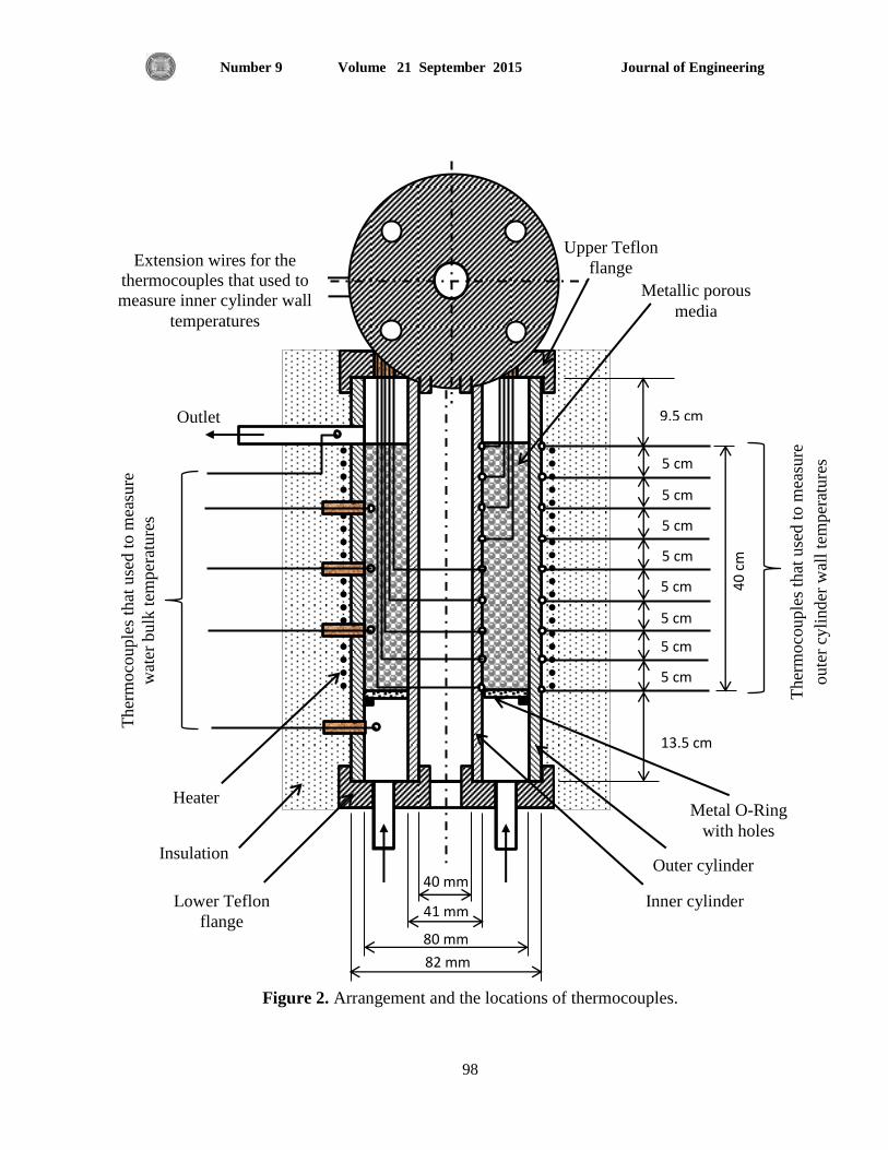
Journal of Engineering Volume 21 September 2015 Number 9
98
Ther
moco
uple
s th
at u
sed
to m
easu
re
oute
r cy
linder
wal
l te
mper
ature
s
Ther
moco
uple
s th
at u
sed
to m
easu
re
wat
er b
ulk
tem
per
ature
s
Insulation
Lower Teflon
flange
Inner cylinder
Outer cylinder
Upper Teflon
flange
Metal O-Ring
with holes
Heater
Outlet
Metallic porous
media
Figure 2. Arrangement and the locations of thermocouples.
5 cm
5 cm
5 cm
5 cm
5 cm
5 cm
5 cm
5 cm
13.5 cm
9.5 cm
40 mm
41 mm
80 mm
82 mm
Extension wires for the
thermocouples that used to
measure inner cylinder wall
temperatures
40
cm

Journal of Engineering Volume 21 September 2015 Number 9
99
Test section
Flowmetr Drain
reservoir
Stand
Water tank
Transformer
Digital
thermometer
Figure 3. Photograph of the experimental apparatus.
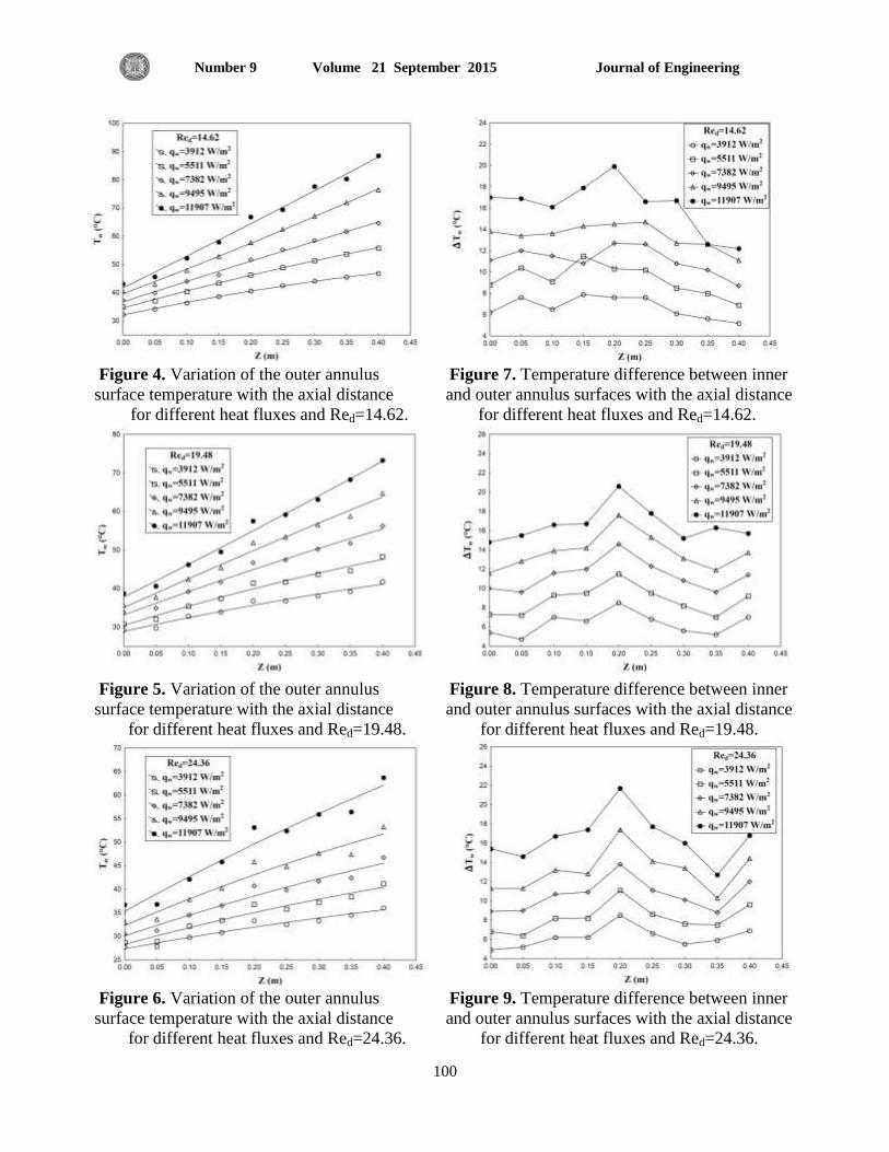
Journal of Engineering Volume 21 September 2015 Number 9
100
Figure 4. Variation of the outer annulus Figure 7. Temperature difference between inner
surface temperature with the axial distance and outer annulus surfaces with the axial distance
for different heat fluxes and Red=14.62. for different heat fluxes and Red=14.62.
Figure 5. Variation of the outer annulus Figure 8. Temperature difference between inner
surface temperature with the axial distance and outer annulus surfaces with the axial distance
for different heat fluxes and Red=19.48. for different heat fluxes and Red=19.48.
Figure 6. Variation of the outer annulus Figure 9. Temperature difference between inner
surface temperature with the axial distance and outer annulus surfaces with the axial distance
for different heat fluxes and Red=24.36. for different heat fluxes and Red=24.36.
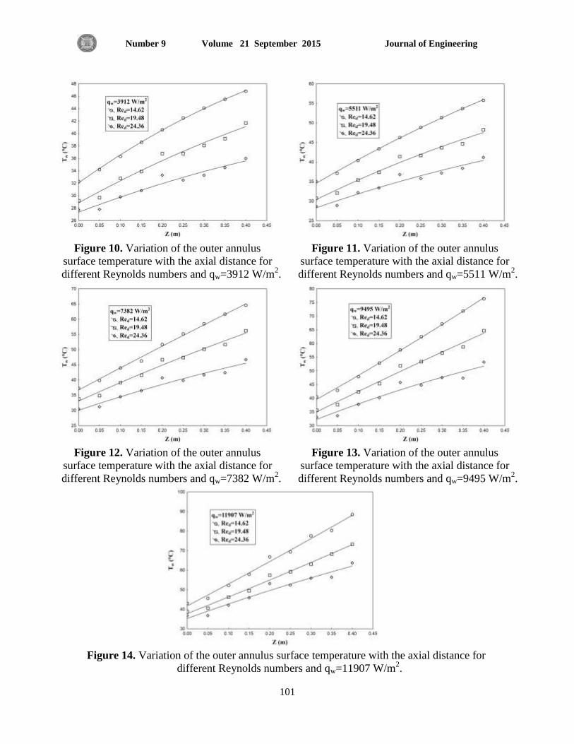
Journal of Engineering Volume 21 September 2015 Number 9
101
Figure 10. Variation of the outer annulus Figure 11. Variation of the outer annulus
surface temperature with the axial distance for surface temperature with the axial distance for
different Reynolds numbers and qw=3912 W/m2. different Reynolds numbers and qw=5511 W/m
2.
Figure 12. Variation of the outer annulus Figure 13. Variation of the outer annulus
surface temperature with the axial distance for surface temperature with the axial distance for
different Reynolds numbers and qw=7382 W/m2. different Reynolds numbers and qw=9495 W/m
2.
Figure 14. Variation of the outer annulus surface temperature with the axial distance for
different Reynolds numbers and qw=11907 W/m2.
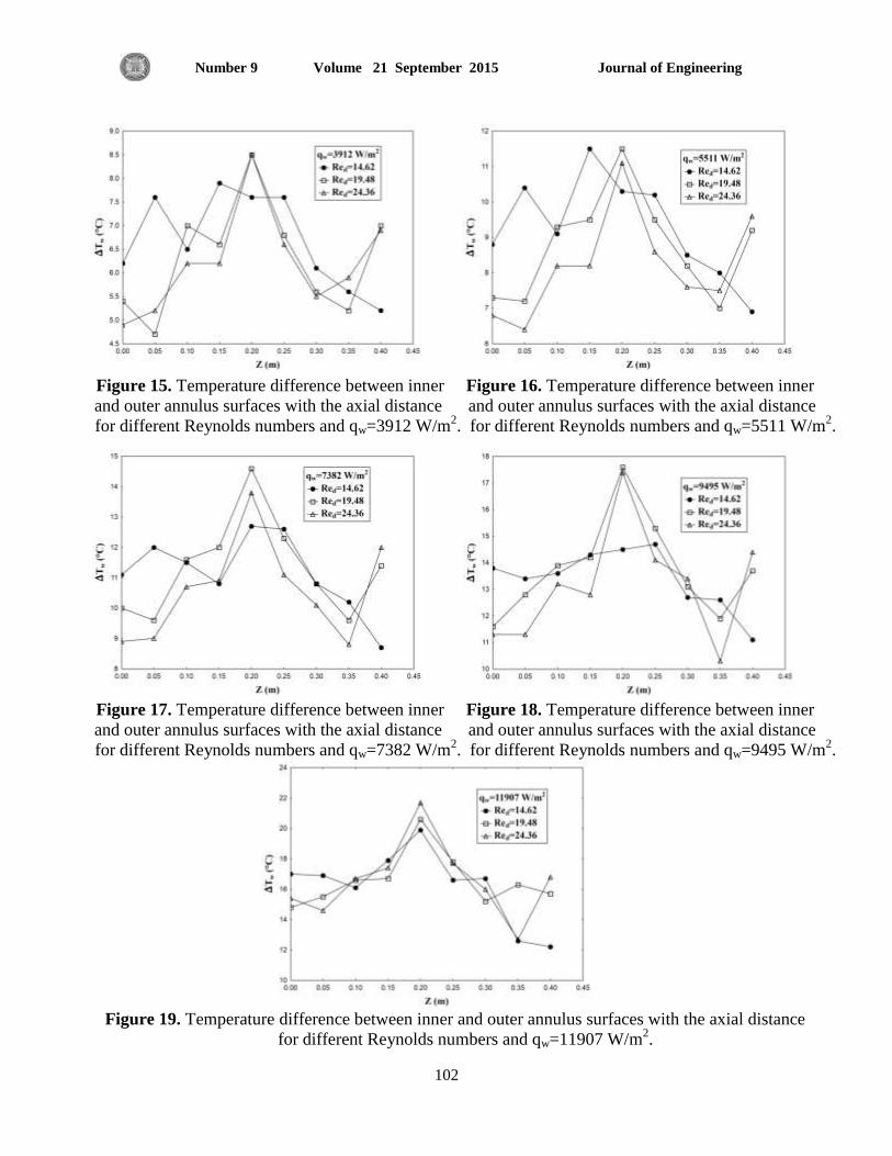
Journal of Engineering Volume 21 September 2015 Number 9
102
Figure 15. Temperature difference between inner Figure 16. Temperature difference between inner
and outer annulus surfaces with the axial distance and outer annulus surfaces with the axial distance
for different Reynolds numbers and qw=3912 W/m2. for different Reynolds numbers and qw=5511 W/m
2.
Figure 17. Temperature difference between inner Figure 18. Temperature difference between inner
and outer annulus surfaces with the axial distance and outer annulus surfaces with the axial distance
for different Reynolds numbers and qw=7382 W/m2. for different Reynolds numbers and qw=9495 W/m
2.
Figure 19. Temperature difference between inner and outer annulus surfaces with the axial distance
for different Reynolds numbers and qw=11907 W/m2.

Journal of Engineering Volume 21 September 2015 Number 9
103
Figure 20. Local heat transfer coefficient with Figure 23. Local heat transfer coefficient with
the axial distance for different heat fluxes and the axial distance for different Reynolds
Red=14.62. numbers and qw=3912 W/m2.
Figure 21. Local heat transfer coefficient with Figure 24. Local heat transfer coefficient with
the axial distance for different heat fluxes and the axial distance for different Reynolds
Red=19.48. numbers and qw=7382 W/m2.
Figure 22. Local heat transfer coefficient with Figure 25. Local heat transfer coefficient with
the axial distance for different heat fluxes and the axial distance for different Reynolds
Red=24.36. numbers and qw=11907 W/m2.
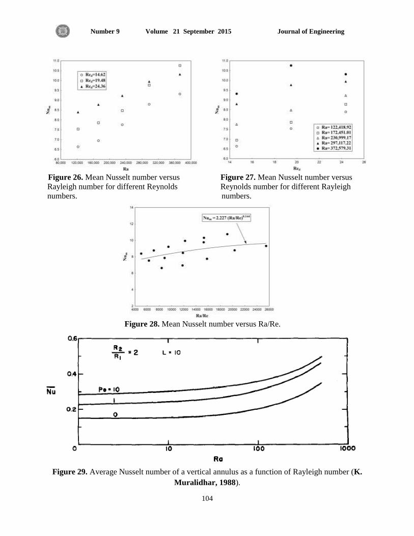
Journal of Engineering Volume 21 September 2015 Number 9
104
Figure 26. Mean Nusselt number versus Figure 27. Mean Nusselt number versus
Rayleigh number for different Reynolds Reynolds number for different Rayleigh
numbers. numbers.
Figure 28. Mean Nusselt number versus Ra/Re.
Figure 29. Average Nusselt number of a vertical annulus as a function of Rayleigh number (K.
Muralidhar, 1988).

Journal of Engineering Volume 21 September 2015 Number 9
169
Effect of Recirculation Ratio on the Uniformity Flow in a High Area Ratio of
Outlets Pipe at Different Entrance flow rates
Dr. Wissam H. Alawee Dr. Jafar M. Hassan Dr. Wahid S. Mohammad
Lecture professor professor
Center of truuing-Univ. of tecnology Mech. Eng. Dep.- Univ.of Technology Mech. Eng. Dep.- Univ. of Technology
[email protected] [email protected] [email protected]
ABSRTACT
The uniform flow distrbiution in the multi-outlets pipe highly depends on the several parameters
act togather. Therefor, there is no general method to achieve this goal. The goal of this study is to
investigate the proposed approach that can provide significant relief of the maldistribution. The
method is based on re-circulating portion of flow from the end of the header to reduce pressure at
this region . The physical model consists of main manifold with uniform longitudinal section having
diameter of 152.4 mm (6 in), five laterals with diameter of 76.2 mm (3 in), and spacing of 300 mm.
At first, The experiment is carried out with conventional manifold, which is a closed-end. Then,
small amount of water is allowed by controling the valve located at the end of the manifold slowly.
The pressure and the flow distribution among the lateral pipes were recorded. Different inlet flows
have been tested and the values of these flows are (625, 790, and 950) l/min. The result reveals that
the conventional header give high non-uniform flow distrbution and the distribution of flow is
greatly improved by using the perposed methods . When the recircluting ratio is of 15%, the non-
uniform coefficient (the stander devation) is reduced from 0.48 to 0.13 which means improves in the
flow distribution by 75%.
Keyword: Flow distribution, manifold, uniform
التذفق ف انبىب متعذد المنافز رو نسبت مساحت عالتتىحذ على التذور إعادة نسبت تأثر
عنذ معذلاث تذفق مختلفت
وحذ شات محمذد. د. جعفر مهذي حسن وسام حمذ علىي د.
رار ذسط اسرأر أس
اىجاؼح اىرنىجح -اىجاؼح اىرنىجح قس اىذسح اىنانح -اىجاؼح اىرنىجح قس اىذسح اىنانح -شمض اىرذسة
الخلاصت
ىزىل. جرغ تشنو ذؤثش اىر اىرغشاخ اىؼذذ ػيى مثش تشنو ؼرذ اىافز رؼذدج الااتة خلاه ىيجشا اىرظ اىرصغ
. اىجشا ذصغ سء ذقيو ا ن قرشحح ىطشقح ذطش اىحاى اىثحث. اىذف زا ىرحقق حذدج طشقح اك ذجذ لا
ز ف اىشذفغ اىضغظ ىرقيورىل ع اىرفش ىلاثب اىغيقح اىاح اىائغ سثح حذدج سحة ػيى اىطشقح ز ذسرذ
76.2) تقطش فشػح ااتة خسح (ي 152.4) تقطش سئس اثب رن قطغ الاخرثاس اىسرخذ ف اىثحث . اىطقح
ي(. أجضخ اىرجاسب ف اىثذاح ػيى قطغ الاخرثاس تاىرص اىرقيذي )اىاح 300ت الااتة اىفشػح ماد ) اىسافح ،ي(
غيقح( تؼذ رىل ر اىساح ىناخ خريفح اىاء اىشس اىاح اىغيقح خلاه صا ذحن ثثد ف اح الاثب.
ة /ثاح. تد اىرائج ا ػيح سح( ىرش950، 790، 625ح اىرذفق اىذاخو خلاه اىرجاسب )ثلاثح ق خريفح ىناسرخذد
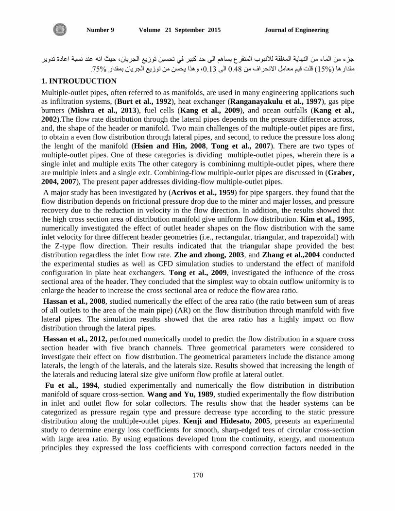
Journal of Engineering Volume 21 September 2015 Number 9
170
جضء اىاء اىاح اىغيقح ىلاثب اىرفشع سا اىى حذ مثش ف ذحس ذصغ اىجشا، حث ا ػذ سثح اػادج ذذش
.75تقذاس % ذصغ اىجشا، زا حس 0.13اىى 0.48( قيد ق ؼاو الاحشاف 15قذاسا )%
1. INTROUDUCTION
Multiple-outlet pipes, often referred to as manifolds, are used in many engineering applications such
as infiltration systems, (Burt et al., 1992), heat exchanger (Ranganayakulu et al., 1997), gas pipe
burners (Mishra et al., 2013), fuel cells (Kang et al., 2009), and ocean outfalls (Kang et al.,
2002).The flow rate distribution through the lateral pipes depends on the pressure difference across,
and, the shape of the header or manifold. Two main challenges of the multiple-outlet pipes are first,
to obtain a even flow distribution through lateral pipes, and second, to reduce the pressure loss along
the lenght of the manifold (Hsien and Hin, 2008, Tong et al., 2007). There are two types of
multiple-outlet pipes. One of these categories is dividing multiple-outlet pipes, wherein there is a
single inlet and multiple exits The other category is combininng multiple-outlet pipes, where there
are multiple inlets and a single exit. Combining-flow multiple-outlet pipes are discussed in (Graber,
2004, 2007), The present paper addresses dividing-flow multiple-outlet pipes.
A major study has been investigated by (Acrivos et al., 1959) for pipe spargers. they found that the
flow distribution depends on frictional pressure drop due to the miner and majer losses, and pressure
recovery due to the reduction in velocity in the flow direction. In addition, the results showed that
the high cross section area of distribution manifold give uniform flow distribution. Kim et al., 1995,
numerically investigated the effect of outlet header shapes on the flow distribution with the same
inlet velocity for three different header geometries (i.e., rectangular, triangular, and trapezoidal) with
the Z-type flow direction. Their results indicated that the triangular shape provided the best
distribution regardless the inlet flow rate. Zhe and zhong, 2003, and Zhang et al.,2004 conducted
the experimental studies as well as CFD simulation studies to understand the effect of manifold
configuration in plate heat exchangers. Tong et al., 2009, investigated the influence of the cross
sectional area of the header. They concluded that the simplest way to obtain outflow uniformity is to
enlarge the header to increase the cross sectional area or reduce the flow area ratio.
Hassan et al., 2008, studied numerically the effect of the area ratio (the ratio between sum of areas
of all outlets to the area of the main pipe) (AR) on the flow distribution through manifold with five
lateral pipes. The simulation results showed that the area ratio has a highly impact on flow
distribution through the lateral pipes.
Hassan et al., 2012, performed numerically model to predict the flow distribution in a square cross
section header with five branch channels. Three geometrical parameters were considered to
investigate their effect on flow distrbution. The geometrical parameters include the distance among
laterals, the length of the laterals, and the laterals size. Results showed that increasing the length of
the laterals and reducing lateral size give uniform flow profile at lateral outlet.
Fu et al., 1994, studied experimentally and numerically the flow distribution in distribution
manifold of square cross-section. Wang and Yu, 1989, studied experimentally the flow distribution
in inlet and outlet flow for solar collectors. The results show that the header systems can be
categorized as pressure regain type and pressure decrease type according to the static pressure
distribution along the multiple-outlet pipes. Kenji and Hidesato, 2005, presents an experimental
study to determine energy loss coefficients for smooth, sharp-edged tees of circular cross-section
with large area ratio. By using equations developed from the continuity, energy, and momentum
principles they expressed the loss coefficients with correspond correction factors needed in the

Journal of Engineering Volume 21 September 2015 Number 9
171
equations. The comparison of the proposed equations with the experimental results obtained by
authors showed that the proposed equations with the correction factors gives good agreement with
the experimental results for the area ratio greater than 8.
The literature survey indicates that a flow uniformity are gaining importance in many engineering
applications. Also, it was found that impossible achieve this goal for conventional header has area
ratio greater than unity (area ratio, AR the ratio between sum of areas of all outlets to the area of the
main pipe). Wissam, 2005, studied numerically and experimentally several methodologies to
improve the flow uniformity in distribution manifold. One of these methodologies were study the
effect of drawing ratio (flow out from closed end of manifold) on the flow distribution at the
manifold diameter of 101.6 mm (4 in). The results showed that the flow drawing from the end of
manifold reduced the flow maldistribution through lateral pipes. The objective of the present study
is to investigate the effect of drawing ratio on the flow distribution at large header diameter 152.6
mm (6 in), different drawing ratio, and different entrance velocities.
2. EXPERIMENTAL SETUP
The test rig of this study is shown in Fig. 1. The rig was built at a selected site in Department of
Machinacl Engineering, University of Technology, Baghdad. The test rig, shown in Figure consists
of the follwing parts: the main supply pipe, test section, shalow tank to collection water, flow meter,
manometer and a centrifugal pump to recycle water to main supply pipe. In order to make a
successful and accurate experimental study using the proposed approach, two test sections are made;
the first one is made according to conventional design with large area ratio. It is simply shaped with
uniform cross section header. The second is made according to the proposed approach. It connected
with a globe valve to investigate the effect downstream outflow on uniformity of flow distribution.
These test sections consist of a manifold with five-lateral pipe orizontal header and five parallel
channels. The header is made of acrylic material to ensure the good visibility of developed flow. It
has 1500 mm long and 152.4mm (6 in) diameter.
The inlet of each test section is connected to a 3500 mm length pipe made of clear polyvinyl
chloride (PVC) at same diameter of test section. The long pipe provides a fully developed flow. The
first test section is dead end where it is closed by a PVC plug. the end of another test section is
connected to globel valve. Each branch has 76.2-mm diameter. The branches are regularly 300-mm
spaced along the header. The diagrames in Fig.2. show the general configuration of the test sections
used.
3. FLOW LOOP AND MEASURING DEVICES
The experimental loop is shown in Fig.3. Water is the test fluid. The water flow rate from each
lateral pipe is collected in a shallow tank, with dimentioin 1500-mm x 1500-mm x 400-mm, then
discharged continuously through pipe with diameter of 152.4 mm (6 in) to recycle water by
centrifugal pump to main supply tank. The water flow rate is measured by five glass containers with
a capacity of 50 liter for each container. The containers are placed on a movable support, which
allows it to move freely at the same time of carrying out of experiments. The containers and support
are shown in Fig.4. Nine pressure tapes are located along the length of the test section. These
pressure tapes are used to measure the pressure head in inlet of manifold and at different points

Journal of Engineering Volume 21 September 2015 Number 9
172
along the length of the distribution manifold. The inlet water to the test section is controlled by a
globle valve and is measured by a target flo.wmeter.
4. EXPERIMENTAL CONDITIONS
The first tests are carried out with the reference geometry (a multiple-outlet pipes with dead end) to
test the effect of the inlet flow rate on the flow distrbution. Inlet flow rates ranges are 625–950
l/min. Three different of drawing ratio are investigated to study its impact on the flow uniformity.
All tests are performed at a room temperature and at a atmosphere pressure.
5. MATHEMATICAL MODEL
Fig. 5 shows The control volume in an dividing manifold. The theoretical flow model for present
work is based on the same mathematical style as that in the previous work (Wang, 2008, Wang,
2011). The mass and momentum balances can be written as follows:
Mass Conservation:
where A and Al are the cross-sectional areas of the header and the lateral pipe, respectively, Wl the
axial velocity in header pipe, Ul the velocity in lateral pipe, Z axial coordinate, L length of the
header, and n number of lateral pipes. Setting ∆X = L/n . Momentum Conservation:
(
) (
)
Where P is pressure in the manifold, D diameter of header pipe, w is given by Darcy–Weisbach
formula, , and . After inserting w and Wl into Eq. (3) and neglecting the
higher orders of ∆X, Eq. (3) can be rearranged as follows:
The flow in the lateral pipes can be described by Bernoulli’s equation with a consideration of flow
turning loss. Hence, the velocity in a lateral pipe, Ul, is correlated to the pressure difference between
the manifold and the ambient as follows:
(
)

Journal of Engineering Volume 21 September 2015 Number 9
173
where Cf is turning loss coefficient from the manifold into the lateral pipes, H is length of the lateral
pipe, dl is diameter of lateral pipe, fl is coefficient of the friction for the lateral pipe. Inserting Eq. (2)
into Eq. (5), gives:
(
)
(
)
Eqs. (4) and (6) can be reduced to dimensionless form using the following dimensionless groups.
(
)
(
)
where W0 is the inlet velocity of the manifold. Inserting Eq. (9) into Eq. (8) and after rearranging,
one obtains an ordinary differential equation for the velocity in the distributon manifold:
(
)
(
)
5.1 Analytical Solution
We define two constants:
(
)
(
)
Thus, Eq. (10) is reduced as follows:
The general solutions of the governing equation (13) for flow distribution in manifold is similar to
that done by Wang, 2008, 2011. To solve Equation (13), we assume that the function, w, is
a solution of Equation (13) and substitute it and its derivatives into Eq. (13), we obtain the
characteristic equation of Equation (13).

Journal of Engineering Volume 21 September 2015 Number 9
174
The solutions of Equation (13) depends on the sign of Q3 + R
2, which have three cases. The
solutions of case (Q3 + R
2 > 0) is listed here.
* √ +
* √ +
√
√
Where * √ +
* √ +
Thus, the general solution of Eq. (13) and boundary conditions can be written as follows:
[ (√ ) (√ )]
The equation of axial velocity in the manifold can be written as follows:
[ (√ )
(√ )]
The equation of velocity of lateral can be written as follows:
(
) *
√ √ √
√ +
Flow distribution through lateral pipe:
(
)
*
√ √ √
√ +
5. RESULTS AND DISCUSSION
According to Hassan et al., 2008 and Wissam, 2015 the flow distribution along multi-outlet pipe
is depended largely on the area ratio. They found that, when the area ratio increases to larger than
unity, the flow distribution along multi-outlet pipe is far from uinform. On the contrary, when the
area ratio decreases, the distribution of flow improves dramatically. Therefore, the present results
are expected for area ratio greater than unity. These results will be a reference to investigate the
effect of proposed approach on the flow and pressure distribution.
The results of the flow rate for each outlet at three different inlet flow rates (625, 790, 950) l/min.
are given in Fig.6. As expected, the water flow in the outlets tends to increase, starting with the first

Journal of Engineering Volume 21 September 2015 Number 9
175
outlet which is badly fed to the last one which is so highly fed (more than twice the mean water flow
rate). In contrast, the pressure distribution along the length of manifold also be uneven.
There is a clear flow maldistribution which can be explained as follows: there are two factors
control the pressure variations in multi-outlet header: friction and momentum. These two factors
work in opposite directions to each other. The friction effect lowers the pressure along the header in
opposing the momentum effect. In tradetional header, the momentum cannot balance the friction
effect, resulting in a non-uniform flow distribution. When the multi-outlet pipe is dead end, water is
recirculating at the closed end. This causes unstable flow and pressure increase, resulting in an
increase in flow rate through branch No.5. This is in agreement with the findings in reference,
Pertorius, 1997.This is in agreement with the results of reference, Pertorius, 1997.
The behavior of flow distribution is consistent with the pressure distributions that have been
displayed in Fig.7. This figure shows that the pressure increases with increasing of downstream
distances. Since the pressure difference drives the per-outlet water flow rate, so it is necessary to
increase the flow rate with downstream distance.
The difficulty in obtaining uniform distribution is due to pressure build-up at the header end. To
reduce the pressure, a portion of the flow is re-circulated to supply tank were carried out. Figs. 8, 9,
and 10 present the results of flow rate at drawing ratios of 5%, 10%, and 15% respectively. From
these figures, it can be seen that the ratio of withdrawal water from the closed end of manifold helps
to a great extent to improve the distribution of the flow regardless of inlet flow rate (in the range
used in the experiment that is from 625 l/min. to 950 l/min.). When the drawing ratio is 0%, it means
that there is no flow from the end of the manifold. In this case, a part of the kinetic energy is
converted to a rise in pressure at that region.Thus, the water flow through the outlets is increasing
towards dead end of the header. When the drawing ratio is certain percentage, the pressure at the
dead end will decrease and hence the water flow from the last outlet is also decreases. When the
drawing ratio increses from 5% to 15%, the pressure along the manifold was become nearly uniform
which gives a better flow distribution through the outlets.
Fig.11 shows the percentage of flow rate fraction for each outlet takes from the total flow at
different drawing ratio. Comparing these results with those of traditional header (closed end), a clear
improvement can be seen in flow distribution. For example, when the traditional header is used, the
discharge from last outlet is about 29.5% of the total flow rate while for the header with 15%
drawing ratio, the percentage is reduced from 29.5% to 22.5%. In other words, the flow discharge
from first outlet is 64% less than that from last outlet but when the header with 15% drawing ratio is
used, this percentage is reduced from 64% to 20%.
The percentage of absolute mean deviation from average flow rate is shown in Fig.12. From this
figure, the values of standard deviation (STD) are 0.48, 0.439, 0.311, and 0.241 at Drawing ratio of
0%, 5%, 10%, and 15%, respectively. The lowest value of (Φ) was of the header with 15% drawing
ratio that corresponding to 0.025. It is clear that water withdrawal in certain proportions from the
high pressure region (in which the kinetic energy is converted to a rise in pressure) would help
reduce pressure in this region, thus resulting in improved flow distribution.
Journal of Engineering Volume 21 September 2015 Number 9
176
A comparison between the present results and the result of Wissam, 2015 shows (see Table 1) that
the selection of drawing ratio depends largely on the header diameter. On the other hand, the total
inlet flow rate does not affect the flow distribution. When the drawing ratio of 10%, the value of
stander deviation is (0.377). Also, when using the same ratio but with header diameter of (6 in), the
value of deviation coefficient is reduces from 0.377 to 0.311.
Experimental tests for flow distribution from manifold have been conducted, which made it
possible to validate the analytical procedures. Fig. 13 shows comparison between the computed and
experimental flow rate per-outlet. It can be clearly seen from the figures that the different of flow
rate between computed and experimental value is acceptable.
5. CONCLUSION
Two test sections representing different header structures were used in this study. The first test
section is uniform header, the second header with drawingratio. In both test sections, the diameter of
the main pipe was 152.4 mm and of the lateral pipe 76.2 mm. the method of withdrawal water from
the dead end of manifold is a very successful approach to improve flow uniformity. where, the flow
distribution is improved by 75% which means the stander devation is reduced from 0.48 to
0.241.Three different values of inlet flow rate of (625, 790,950) l/min had been used in the
experiments. From the results, it is found that change in the total flow rate has a slight effect on flow
uniformity. Therefore, it can be safely said that the inlet flow rate has no effect on flow distribution.
ACKNOWLEDGEMENTS
The authors would like to thank the Mechanical Engineering depertment, University of technology
for its assistance.
REFFERENCE
Acrivos, A., Babcock, B.D., and Pigford, R.L., 1959. Flow distribution in manifolds. Chem.
Eng. Sci. vol. 10, pp. 112–124.
Alawee, W. H., 2015, Solution Methodologies for the Fluid Flow Distribution Manifold
Problem, Ph.D Thesis, Department of Mechanical Engineering, University of Technology,
Iraq.
Burt, C. M., Walker, R. E., Styles, S. W., 1992, Infiltration System Evaluation Manual.
Irrigation Training And Research Center,. California polytechnic state, Univcity San Luis
Obispo, CA.
Bleninger, T., Lipari, G., and Jirka, G., 2002, Design And Optimization Program For Internal
Diffuser, 2nd Int. Conf. on Marine Waste Water Discharges, MWWD 2002.
FU H., Watkins, A. P., and Yianneskis M., 1994, The Effects Of Flow Split Ratio And Flow
Rate In Manifolds,. Int. J. Numerical Methods in Fluids, vol.18, no.9, pp. 871-886.

Journal of Engineering Volume 21 September 2015 Number 9
177
Graber, S. D., 2004, Concepts of spatially varied flow.” Proc., HTFED, 2004 ASME Heat
Transfer/Fluids Engineering Summer Conf., ASME, New York.
Graber, S. D., 2007, Full-flowing collection conduits with nonuniform inflow.” Journal.
Environment Engineering, vol. 133, no. 6, pp. 575–580.
Hassan, J. M., Mohamed, T. A., Mohammad, W. S., and Alawee,W. H., 2014, Experimental
and Numerical Study on the Improvement of Uniformity Flow for Three-Lateral Dividing
Manifold, World Research & Innovation Convention on Engineering & Technology,
Putrajaya, Malaysia, 25-26 November 2014.
Hsien-Ter Chou and Hin-Chi Lei, 2008, Outflow Uniformity along a Continuous Manifold,
Journal of Hydraulic Engineering,ASCE / SEPTEMBER 2008 , pp. 1383-1388.
Hassan, J. M.,208, Flow Distribution in Manifolds, Journal of Engineering and
Development, vol. 12, no.4, pp. 159-177.
Hassan, J. M., 2012, Study of Three Dimensional Fluid Flow in Manifold-Laterals System,
Eng. & Tech. Journal, vol.30, no. 7,pp. 1132-1148.
Kang, S., Min, K., Mueller, F., and Brouwer, J., 2009, Configuration effects of air, fuel, and
coolant inlets on the performance of a proton exchange membrane fuel cell for automotive
applications, International Journal of Hydrogen Energy, vol.34, no.16, pp. 6749–6764.
Kim, S., Choi, E., and Cho, Y.I., 1995, The effect of header shapes on the flow distribution in
a manifold for electronic packaging applications, International Communicationsin Heat and
Mass Transfer, vol. 22, pp. 329-341.
Kenji, O., Hidesato, I., 2005, Energy Losses at Tees with Large Area Ratios, Transactions of
the ASME, Journal of Fluids Engineering, Vol. 127, pp. 110-116.
Mishra, N. K., Muthukumar, P., and Mishra, S. C., 2013, Performance Tests on Medium-
Scale Porous Radiant Burners for LPG Cooking Applications, International Journal of
Emerging Technology and Advanced Engineering Vol. 3, Special Issue 3, pp. 126-130.
Pertorius W.A., Dividing- flow Manifold Calculations with a Spreadsheet, water science, 23
(2) (1997) 147-150.
Ranganayakulu, Ch., Seetharamu, K. N., and Sreevatsan, K.V., 1997, The Effects of Inlet
Fluid FlowNonuniformity on Thermal Performance and Pressure Drops in Crossflow Plate-
fin Compact Heat Exchangers, Int. J. Heat Mass Transfer, vol. 40, no. 1, pp. 27–38.
Tong, J.C.K., Sparrow, E.M., Abraham, J.P., 2007, Attainment of flowrate uniformity in the
channels that link a distribution manifold to a collection manifold, Journal Fluids
Engineering, vol. 129, pp.1186–1192.
Tong, J.C., Sparrow, E.M., and Abraham, J.P.,2009, Geometric strategies for attainment of
identical outflows through all of the exit ports of a distribution manifold in a manifold
system, Appl. Therm. Eng., vol. 29, pp. 3552–3560.
Zhe Z., Yan-zhong, L., 2003, CFD simulation on inlet configuration of plate-fin heat
exchangers, Cryogenics, vol. 43, no. 12, pp. 673-678.

Journal of Engineering Volume 21 September 2015 Number 9
178
Zhe, Z., Yan-zhong, L., and Qing, X., 2004, Experimental research on the effects of
distributor configuration in plate-fin heat exchangers, Heat Transfer-Asian Research, vol. 33,
no.6, pp. 402.
Wang, X. A. and P. Yu, Isothermal flow distribution in header systems, International Journal
of Solar Energy, 7(1989)159-169
Wang J., Pressure drop and flow distribution in parallel-channel configurations of fuel cells:
U-type arrangement, International journal of hydrogen energy, 33( 2008 ) 6339 – 6350.
Wang, J., Theory of flow distribution in manifolds, Chem. Eng. J., 168 (2011)1331–1345.
7. NOMENCLATURE
Cf = coefficients of turning losses.
D= diameter of manifold, m.
dl = diameter of the lateral pipe, m.
f =friction factor
A, Al = cross-sectional area of manifold and lateral pipe, m2.
H= length of lateral pipe, m.
L= length of manifold, m.
n = numbers of lateral pipes.
Pa = ambient pressure
pa = dimensionless ambient pressure
P = pressure in manifold
P = dimensionless pressure.
Q = coefficient in Eq. (13), defined by Eq. (11)
R = coefficient in Eq. (13), defined by Eq. (11)
r, r1, r2 = roots of characteristic equation.
W = velocity in manifold (m/s)
w =dimensionless velocity in manifold.
Ul = velocity of lateral pipe, m/s.
ul = dimensionless velocity of lateral pipe.
vc =dimensionless volume flow rate in lateral pipes.
β = average velocity ratio in manifold (Wl/W)
ρ = fluid density (kg/m3)
τw = wall shear stress (N/m2)
ζ = average total head loss coefficient for port flow

Journal of Engineering Volume 21 September 2015 Number 9
179
Table 1. A comparison of the results obtained in the present study with those of Ref.,
Alawee,2015.
Researcher Drawing
ratio, %
Percentage of flow rate fraction for each outlet
takes from the total flow
Outlet
1
Outlet
2
Outlet
3
Outlet
4
Outlet
5 STD
Wissam, 2015
Header diameter=101.6 mm
(4″)
8 11% 15% 12% 22% 22% 0.371
10 11.9 16.6 23.1 23.6 24.8 0.354
The present work
Header daimeter=152.6 mm
(6″)
10 13.3 16.6 22.0 23.8 24.1 0.311
15 14.6 18.5 21.0 21.4 21.9 0.241
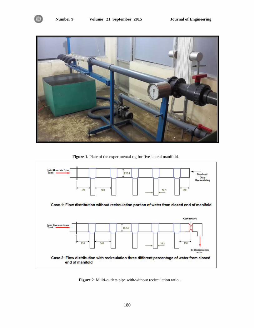
Journal of Engineering Volume 21 September 2015 Number 9
180
Figure 1. Plate of the experimental rig for five-lateral manifold.
Figure 2. Multi-outlets pipe with/without recirculation ratio .
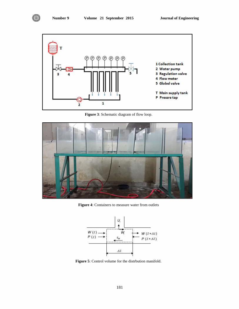
Journal of Engineering Volume 21 September 2015 Number 9
181
Figure 3: Schematic diagram of flow loop.
Figure 4: Containers to measure water from outlets
Figure 5: Control volume for the distrbution manifold.

Journal of Engineering Volume 21 September 2015 Number 9
182
0
50
100
150
200
250
300
350
0 1 2 3 4 5 6
Flo
w r
ate
l/m
in
Branch no.
Qinlet=950 l/min.
Qinlet=790 l/min.
Qinlet=625 l/min.
0
50
100
150
200
250
300
350
0 1 2 3 4 5 6
Flo
w r
ate
l/m
in
Branch no.
Qinlet=950 l/min.
Qinlet=790 l/min.
Qinlet=625 l/min.
Header diameter = 152.4 mm lateral diameter = 76.2 mm
Figure 6: Flow distribution plot at three value of inlet flow water .
0
10
20
30
40
50
60
70
0 0.2 0.4 0.6 0.8 1 1.2 1.4 1.6
Pre
ssre
he
ad,
cmH
2O
Header Length (m)
Qinlet=950 l/min.
Qinlet=790 l/min.
Qinlet=625 l/min.
Figure 7: Variations of pressure head along the manifold .
Drawing Ratio=5%
Figure 8: Flow distribution plot of manifold with 5% drawing ratio at
three value of inlet flow water .

Journal of Engineering Volume 21 September 2015 Number 9
183
0
50
100
150
200
250
300
0 1 2 3 4 5 6
Flo
w r
ate
l/m
in
Branch no.
Qinlet=950 l/min.
Qinlet=790 l/min.
Qinlet=625 l/min.
Drawing Ratio=10%
Figure 9: Flow distribution plot of manifold with 10% drawing ratio at
three value of inlet flow water .
0
50
100
150
200
250
300
0 1 2 3 4 5 6
Flo
w r
ate
l/m
in
Branch no.
Qinlet=790 l/min.
Qinlet=950 l/min.
Qinlet=625 l/min.
Drawing Ratio=15%
Figure 10: Flow distribution plot of manifold with 15% drawing ratio at
three value of inlet flow water.
Figure 11: Flow rate fraction at three value of drawing ratio.
0
5
10
15
20
25
30
35
40
0 1 2 3 4 5 6
Flw
oFr
acti
on
, %
Branch no.
Dead end
Rec. Ratio=5 %
Rec. Ratio=10 %
Rec. Ratio=15 %

Journal of Engineering Volume 21 September 2015 Number 9
184
0
50
100
150
200
250
300
Lateral 1 Lateral 2 Lateral 3 Lateral 4 Lateral 5
Flo
wra
te l/
min
Lateral no.
Experimental
Analytical
Figure 12: Percentage of absolute mean deviation from average for three drawing ratio
0
5
10
15
20
25
30
35
40
45
50
55
60
0 5 10 15 20
Stan
dar
d d
evi
atio
n
%
Drawing Ratio
STD
Figure 13: flow distribution per lateral pipe for manifold

Journal of Engineering Volume 21 September 2015 Number 9
74
Cost of Optimum Design of Trunk Mains Network Using Geographical
Information System and Support Programs
Asst. Prof. Abdul Kareem Esmat Zainal Asst. Lect. Layla kais Abbas
Department of Civil Engineering Department of Surveying Engineering
College of Engineering College of Engineering
Baghdad University Baghdad University
Email: [email protected] Email: [email protected]
ABSTRACT
Sewer network is one of the important utilities in modern cities which discharge the sewage
from all facilities. The increase of population numbers consequently leads to the increase in
water consumption; hence waste water generation. Sewer networks work is very expensive and
need to be designed accurately. Thus construction effective sewer network system with
minimum cost is very necessary to handle waste water generation.
In this study trunk mains networks design was applied which connect the pump stations together
by underground pipes for too long distances. They usually have large diameters with varying
depths which consequently need excavations and gathering from pump stations and transport the
sewage to final waste water treatment plant. This situation urges to decrease the cost to minimum
with efficient design of its performance. The aim of this research is minimizing the cost of all
sewer components of trunk mains which are lengths, diameters, and volume of excavation with
maintaining its performance.
In this research, the utilization of GIS (Geographical Information System) software and VBA
(Visual Basic for Application) which is integrated with GIS was used to implement the MST
(Minimum Spanning Tree) algorithm to create a visual basic computer program that was used to
find the minimum total lengths of the trunk mains in a sewer network.
This method was applied on selected areas in Al-Mansour municipality where there is an
existing sewer system containing trunk mains and pump stations. Total lengths of the existing
trunk mains are calculated and later, the proposed method was implemented to find the minimum
total lengths, with a difference in total lengths of (12601 m).
The new network used to design a proposed sewer system using the computer program
SewerGemsV8i, which can be integrated with GIS. New pipes diameters and slopes were
calculated by supplying the necessary information that is needed by the computer program.
New sewer system was designed which gave more reliable and economical aspects than the
existing one. These results clearly show that when comparing the costs.
Key words: GIS, optimum design, trunk mains, pump stations, minimum cost.

Journal of Engineering Volume 21 September 2015 Number 9
84
كلفت التصوين الاهثل لشبكت انابيب الوجاري بإستخذام نظن الوعلىهاث الجغرافيت والبراهجياث السانذة
م.م. ليلى قيس عباس أ.م.عبذ الكرين عصوج زينل
قسن هنذست الوساحت قسن الهنذست الوذنيت
الهنذست / جاهعت بغذاد كليت كليت الهنذست / جاهعت بغذاد
الخلاصـــــــــــــــــــــــــــــت
ذؼذ شثىاخ اداس ا اث ارسر١ح ثذ ار ذم تخذح ػ ااط ترصش٠ف ١ا اداس ااصي اصاغ
فا ص٠ادج اسرلان ااء إد٠ا ا ص٠ادج ذصش٠ف ١ا اداس. وافح الاشطح اس٠١ح، ظش ض٠ادج ػذد اسىا تارا
اشاء شثىاخ اداس ػ ىف خذا ٠سراج ا اذلح ف ارص١، فأػذاد ذصا١ شثىاخ اداس سماذا راخ وفاءج
اػ ف اؼ راخ وف ال ف الاشاء ظشس ؼادح ذصش٠ف ١ا اداس.
سطر اذساسح ذ اخز ذص١ شثىاخ الاات١ة االح ار ذشتػ سطاخ اعخ غ تؼعا تاات١ة غ٠ح رذج ذسدف ز
اػاق خرفح ذم تدغ ١ا اداس وافح اسطاخ ما ا سطح اؼاح الاخ١شج، ػادج الطاس وث١شج تالأسض
ت١ة تأل وفح غ ظا وفاءج اؼ.اذف ز اذساس زساب اىفح تز اساح وا الاخة ذص١ ذه الاا
غاي، الألطاس، عػاق اسفش، عػذاد سطاخ اعخ، الغ الأفع الاالال ى ػاصش شثىح الاات١ة االح ار ذرع
سطاخ از ٠إثش ػ وفح ز الاات١ة اداؤا.
اؼاخ اسرخذا تشاح ظا اؼاخ ادغشاف١ح تشاح اف١داي ت١سه اذح غ ظااػرذ ف زا اثسث ػ
( Minimum Spanning Tree( از اسرخذ رف١ز خاسص١ح شثىح راخ ال ارذاد ) GIS-VBAادغشاف١ح تا ٠س )
الح.ذى٠ تشاح ٠م تا٠داد ال دع اغاي شثىح الاات١ة ا
ذ اخز تؼط ااغك ظ زذج تذ٠ح اصس وطمح ذساسح رطث١ك اثشاح ذ ذسذ٠ذ الغ سطاخ اعخ ار
ذخذ ذه اطمح سس شثىح ذث و اشاسع ار ى ا ٠مرشذ ف١ا اشاء اات١ة الح ذف١ز اثشاح سساب الصش
ذشتػ ت١ الغ سطاخ اعخ ، ز١ث زظ افشق تالاغاي ت١ الاات١ة افزج الاات١ة دع اغاي ره اشاسع ار
رش(.10621امرشزح تاسرخذا اثشاح )
تشاح GISث اػراد ذه اشثىح امرشزح اسرخذاا ف ازذ تشاح ذص١ شثىاخ اداس اذح غ تشاح
SewerGemsV8i ال الطاس ىح لاات١ة االح زساب ال ١ ى ز الاات١ة تارا اسصي غشض زساب
ػ ال و١اخ سفش٠اخ زظ ا٠عا افشق ت١ الطاس الاات١ة امرشزح ا١ي اخاصح تا.
ف اصس اخدج ع اسررح ع ذف١ز اطشق امرشزح اػط ساح تإ٠دات١ح وث١شج ف ذص١ ذس١ عظح اصش
ادذ٠ذج.
.وفح الاات١ة االح،سطاخ اعخ، الظ اؼاخ ادغشاف١ح، ارص١ الأث, : الكلواث الرئيسيت

Journal of Engineering Volume 21 September 2015 Number 9
84
1. INTRODUCTION
Sewerage pipeline networks is one of the essential infrastructures of the modern cities and it is
very important in serving all people in their houses, factories, hospitals, schools and other vital
utility activities by getting rid of unwanted waste water and water environment prevention.
In recent years, the population has increased significantly, commercial and industrial activities
have also grown dramatically. This has led to an increase in water consumption and
consequentially increases in quantity of wastewater, so there is need to construct a new sewer
networks in areas that suffered from decrease of discharge of waste water.
Design of sewer system includes layout of sewer network, finding lengths, diameters, depths of
all pipes, in addition to finding the best locations of other sewer system components such as
outfall, manholes, pump stations, etc.
Efficiency and good performance are required in the design of sewer network hence it is not an
easy work, in addition it is expensive work; hence need to minimizing and decreasing of
construction and operation costs to the minimum.
1.2 GIS Applications in Sewer Networks
GIS are powerful and cost effective tools for deigning intelligent maps for water, wastewater,
and storm water systems. Effective waste and storm water management requires linking of
specialized computer models to the GIS. Also, integration of engineering, environmental, and
socioeconomic objectives into waste and storm water management could be included.Most of the
physical, social and economic problems associated with waste and storm water are attributable to
unwise land use, insufficient attention to land drainage in urban planning, and ineffective
updating of existing waste and storm water control systems, Rusko et al., 2010.
Typical applications of GIS for waste and storm water systems include: (1) Watershed storm
water management, (2) Floodplain mapping and flood hazard management, (3) Hydrologic and
hydraulic modeling of combined and storm sewer systems, including estimating surface
elevation and slope from digital elevation model data (DEM), (4) Documenting field work, (5)
Planning, assessment of the feasibility and impact of system expansion, (6) Estimating storm
water runoff from the physical characteristics of the watershed, e.g. land use, soil, surface
imperviousness and slope Shamsi, 2002 and Paul Longley, 1999.
Various spatial data layers can be combined and manipulated in a GIS to address planning,
operation, and management issues. For example, water and sewer line information can be
combined with population statistics and ground elevation data to assess the adequacy of water
and sewer utilities, Shamsi, 2005.
2. THE OBJECTIVE OF THE RESEARCH
Trunk mains extents for long distances under the ground, these trunk mains usually have large
pipe diameters, and since they connect many pump stations, they are embedded deeply under the
ground surface for their protection. The design of these trunk mains will be very expensive and
need to be reduced with maintaining accuracy and efficiency in its performance. So the aim of
this research is to find the optimum design of trunk mains network which implement the highest
efficiency and minimum cost. This aim achieved by minimizing the cost of the sewer system
components that includes:

Journal of Engineering Volume 21 September 2015 Number 9
05
i. Length of trunk mains, ii. Trunk mains diameter, and iii. Volume of excavation.
3. METHODOLOGY OF THE WORK
This research developed a methodology in the trunk mains design method that depend on graph
theory algorithm to find the minimum total lengths of trunk mains which is Minimum Spanning
Tree (MST); it was programmed in Visual Basic for Applications (VBA) which is integrated
with GIS, this algorithm was implemented on some selected areas in Baghdad city to give
minimum total pipe lengths.
Bentley SewerGEMs V8i program is one of computer program that could be integrated with GIS
to compute the appropriate pipe diameters and slopes that affect the trunk mains pipes depths.
4. MINIMUM SPANNING TREE ALGORITHM
Using graph algorithm MST is very powerful in providing the tree that connects all nodes of a
Graph (which are represented by pump stations in this research) with minimum length of edges
(which are represented by the pipe lines connecting the pump stations), the root of the tree is the
disposal location of the waste water. It is necessary to use this algorithm and obtain a tree shaped
network because there will be only one root for this tree which is the location of waste water
disposal and the other branches of the tree represent the links between pump stations. A
minimum spanning tree is so named because it is constructed from the minimum of number of
edges (lines) necessary to cover every node and it is in tree form because the resulting graph is
acyclic (i.e. with no cycles). The minimum spanning tree depends entirely on the starting node.
Michael Mcmillan, 2005.
From the researchers have studied the MST algorithm and its applications is Jason
Eisner, 1997 who explained that the classic "easy" optimization problem is to find the minimum
spanning tree (MST) of a connected, undirected graph. Good polynomial-time algorithms have
been known since 1930. This work reviews those methods, building up strategies step by step so
as to expose the insights behind the algorithms. Implementation details are clarified, and some
generalizations are given. And Paola Flocchini et al., 2007 deduced that in many network
applications the computation takes place on the minimum-cost spanning tree (MST) of the
network G; unfortunately, a single link or node failure disconnects the tree.
5. SEWER SYSTEM DESIGN AND ANALYSIS USING GIS
5.1 Case Study
A sample districts in the west of Baghdad/Iraq city located in the municipality of Al-Mansour
was taken as a case study for implementation the MST to obtain the minimum cost of trunk
mains pipes construction and using SewerGEMs to complete the sanitary design. Fig. 1 shows
the satellite image that shows the sample districts was taken as a case study in municipality of
Al-Mansour with the number of districts.
5.2 The Data Sources
In this research, the required data were gathered from different source, such as shapefile forms,
satellite images, maps, and numerical tables from various resources, which are:

Journal of Engineering Volume 21 September 2015 Number 9
05
Shape file includes all main streets in municipality of Al-Mansour from department
of GIS in Mayoralty of Baghdad (MOB) projected by Universal Transfer Mercator
(UTM) and the spheroid is world geodetic system 84 (WGS84), Zone 38 N.
Shape file includes the locations of all pump stations in municipality of Al-Mansour
from department of GIS in Baghdad Sewage Directorate (BSD) in (MOB) projected
by Universal Transfer Mercator (UTM) and the spheroid is WGS84, Zone 38 N.
Information about diameters and path of existing trunk mains which connect pump
stations together in municipality of Al-Mansour was obtained from BSD.
Information about each pump station, such as discharge, depths of wet-well was also
obtained from BSD.
Satellite image of Bagdad city with resolution of 60 cm was obtained from Quick
Bird satellite.
Fig. 2 shows a satellite image of the study area in Al-Mansour municipality, and also shows the
locations of pump stations (yellow rectangles) and the main streets (red lines), where each pump
station is shown with a label of its name. Fig. 3 shows the satellite image that shows existing
sewer network of trunk mains in the municipality of Al-Mansour.
5.3 Existing Sewer Network
For the analysis of already existing network, collecting some necessary data needed to this study
such as:
1. Ground elevation of Pump stations.
2. Waste water inflow to each pump station.
3. Path of the existing trunk mains, and
4. Trunk mains diameters.
5.4 Obtaining Ground Elevations
Source of the elevations that is depended in this research is from Baghdad Sewage Directorate
(BSD). These elevations were produced by the Japanese Nippon Koie company, and were
obtained in a shape file form. Fig. 4 shows the satellite image that show point's network of the
case study. Any point in these data has ground elevation in addition to Cartesian coordinates (X
and Y).These points can be converted to terrain surface using ArcMap10 by interpolation these
points by IDW method to product Digital Elevation Model (DEM). Fig. 5 shows the satellite
image that shows Digital Elevation Model (DEM) of the districts in municipality of Al-Mansour.
5.5 Waste Water Flow
Waste water flow information was obtained from Baghdad Sewage Directorates (BSD). Each
pump station inflow is shown in Table 1 in cubic meter per day (m3/day). This table also shows
elevations of the pump stations.
5.6 Lengths of the Existing Trunk Mains

Journal of Engineering Volume 21 September 2015 Number 9
05
Fig. 3 showed the existing trunk mains that are in service, where the total lengths of the trunk
mains have a sum of (44895.95 m) which was calculated using ArcGIS computer program. The
depth of these trunk mains ranged generally from 3 m at the start of the pump station and ends at
8 m reaching the next pump station where the waste water level is raised using pumps to 3 m
again. Trunk mains pipes lengths, diameters, and start depths and end depths are shown in table
2;additionally table 2 shows the calculations of the soil excavations in cubic meters (m3) and the
cost of the excavations. These calculations are necessary to obtain the approximate costs that will
be used later for comparison with the new proposed method.
5.7 Pipes Diameters
Pipes diameters are an important factor that affects the cost of the sewer system. The pipes
diameters contribute in the cost in two ways; first, the cost increases with the increase of the pipe
diameter, and second, the pipe diameter affects the width of the excavations, consequently
affecting the excavations cost.
5.8 Pipes Material
The cost also depends on the type of the material used for the pipes in trunk mains. There are
five types of materials usually used for sewer trunk mains, and these types are as following:
Ductile Iron Cement Lined (DICL),
Unplasticised, Modified and Oriented Polyvinyl Chloride (PVC),
Glass Reinforced Plastic (GRP),
Steel Cement lined (SCL) (special applications only),and
Polyethylene (PE) (Less than 100 mm internal diameter only).
The material of these pipes material are used in the districts under study is assumed the UPVC,
the cost per unit length and the approximate total cost of the UPVC pipes for each used diameter
is shown in table 3.The calculations which are shown in table 2 give the approximate value of
the total volume of the excavations in addition to an approximate cost for the
excavations.Adding the cost of the pump stations to this cost gives us the total sewer system cost
for the districts under the case study. This cost can be easily obtained approximately by
multiplying the cost of one pump station by the total number of pump stations as follows:
Total cost of pump stations = No. of pump stations Cost average of a pump station
Total cost = 23 3,000,000,000 = 69, 000,000,000 I.D.
The total cost of a sewer network is calculated and shown in table 4.
5.9 Design of the Proposed Network
Minimizing the total cost can be obtained by minimizing the three items which are: Length of
trunk mains, Trunk mains diameter, and Volume of excavation. The design procedure can be
implemented via the following steps.
5.9.1Obtaining the minimum pipe lengths

Journal of Engineering Volume 21 September 2015 Number 9
05
Obtaining the minimum trunk mains length can be achieved by implementing Minimum
Spanning Tree (MST) algorithm. To implement the new proposed algorithm for network design,
it is required to draw a complete streets network graph that connect almost every point which
represents a pump stations to all other neighboring points (or other pump stations) in the districts
as shown in Fig. 6.
These complete streets network represent all main streets in the districts which are connected to
pump stations and represents a candidate path for trunk mains. The total length of the complete
streets network was (94091.48 m).
Based on Visual Basic for Application (VBA) which integrated in GIS program a new scripting
was designed to find the minimum total lengths of the streets by implementing the MST
algorithm. This code execution can be done by pressing the command button added to the
toolbar of the ArcGIS program as shown in Fig. 7, denoted by the small red circle.
When pressing the command button, a series of commands will be executed that asks for the
required data to implement the algorithm and obtain the required solution, which are the streets
with minimum total lengths.
As soon as the file is stored, the minimum streets network will be shown in the ArcGIS display
area. Fig. 8 shows the minimum spanning streets lengths that connect all pump stations together
and provide the minimum required path for the waste water disposal. The total length of the
streets network is (32294.10 m). Table 5 shows the new total length of streets network.
A simple comparison between the two networks in Fig. 3and Fig. 8 shows the difference in total
lengths of (44895.95 – 32294.10 = 12601.51 m) which saves more than twelve kilometers of
pipe lengths and excavation efforts which has a great economical effect on the total cost of the
sewer system.
5.9.2 Design of sewer system
In the previous sections, the design and layout of the sewer pipes was obtained. The inflow of the
waste water was already obtained as shown in table 1.The sanitary design will be carried out
including the design of the pipe diameters, slopes, and required depths.
The computer program SewerGEMs V8i was used for this purpose as it can integrate with
ArcGIS program and provide the sewer design environment in the ArcGIS environment, which
means it can read the shape file of the new proposed street network and use it for the sewer
system design.
The layout of the conduits is shown in Fig. 9 which also shows that the pump stations, the pump
station usually contain a) Wet-well, b) Pump or pumps battery, and c) Ductile iron pipes to uplift
the waste water under pressure to a higher level and let it flow again under gravity till it reach the
next pump station or the treatment plant. A larger scale of some sample pump stations is shown
in Fig. 10, where the wet-well, the pump, and the pressure pipes combinations are drawn. A
detailed schematic drawing of one pump station is shown in Fig. 11.

Journal of Engineering Volume 21 September 2015 Number 9
08
5.9.3 Computer program components
The next step is to prepare the appropriate data required for modifying the properties of the
components of the sewer system, which includes:
1) Pump stations data: Elevations of pump and inflow quantities are already mentioned in
Table 4. Depth of its will be initially 2 m. These values will be considered in the design
of the new sewer network.
2) Conduits data: Conduits data can be represents the gravity pipes are represented as
follows:
a. Lengths: already found from minimum streets network.
b. Type: UPVC pipes will be considered as it is typically used for the construction
of trunk mains.
c. Diameters: The initial pipe diameters used is 200 mm which is the smallest
diameter; this diameter size will change automatically by the computer program
as needed in the design procedure.
d. Inlet and outlet elevations: the inlet elevation is taken from the manhole attached
to the starting side of the pipe while the outlet elevation is taken from the wet-
well that is at the end of the pipe.
3) Outfall data: (End point of sewer system e.g. treatment plant). The last point that was
considered as the outfall is the al-Kadisiya pump station, because of the limitation of the
area under study (actually, the Al-Kadisiya pump station convey waste water to other
station).
4) Outfall data The last point that was considered as the outfall is the al-Kadisiya pump
station, because of the limitation of the area under study (actually, the Al-Kadisiya pump
station convey waste water to other station
5) Pressure Pipe: Pressure pipes are the link between the wet-well and the pump from one
side and the link between the pump and the manhole from the other side, as the waste
water flows from the wet-well through the pump to the next manhole. All pressure pipes
were given a length of 300 mm (as recommended by the instructions of the sewer GEMs
program manual), ductile iron material, and a diameter of 150 mm was taken as an initial
value
5.9.4 Sewer GEMs program run
The computer program has two calculation alternatives, the first, is the design alternative, and
the second is the analysis alternative.
The design alternative is the first choice where the computer program performs the design
procedure regarding all constrains that were already supplied to the calculation options including
the slope constrains (0.001 – 0.1), cover constrains (0.7m – 10m), and velocity constrains (0.61
m/sec – 4 m/sec) (as recommended by the instructions of the computer program manual).
The design was done for steady state condition neglecting the variation of the amount of waste
water during the day (24 hrs.), only peak values were taken into consideration in the design
procedure.
The results obtained from the design procedure affect the pipes diameters, slopes of pipes, and
cover constrains. Minor adjustments were made at the analysis phase of the program including
pipe invert level to maintain slopes within constrains.

Journal of Engineering Volume 21 September 2015 Number 9
00
Results of computer program run is shown in table 6 which also includes the necessary
calculations for the amount of excavations and its cost, while table 7 shows the calculations of
pipe costs considering the reduced lengths of pipes and its diameter which reflects the reduced
cost. After the result was taken it can be compute the total cost of proposed sewer network as
shown in table 8 and the table 9 that shows the comparison between the costs and the reduction
obtained using the proposed network.
6. DISCUSSION& CONCLUSION
A. MST provides a successful solution for obtaining the minimum total lengths of trunk
mains pipes, those pipes usually are large in diameters, they run for long distances and
may go deep into the ground, consequently, they may cost a lot according to these
factors, so any reduction in these costs may reduce the overall cost of the system.
B. MST algorithm can be very useful in estimating the paths for trunk mains (or any large
pipes may be used in sewer systems) as any reduction may be obtained is reflected
directly on the total cost of the sewer system.
C. After obtaining the MST, the integrated computer program (SewerGems) with the GIS
program, can facilitate the sewer system design or analysis. This computer program
takes the required information directly from the ArcGIS map. The trunk mains pipes
lengths and pump stations locations are obtained through "Model Builder" command in
the SewerGEMs menu.
D. Other hydraulic design operations are carried out by the computer program after all the
complimentary information is supplied (e.g. hydraulic constrains, velocities, minimum
and maximum cover, slopes, etc.).
E. The computer program (SewerGEMs) can work either in design mode or analysis mode.
It depends on the required operation by the user. Usually a design process is carried out
first then any required adjustments may be carried out then an analysis process is then
worked out to see the effect of these adjustments. This operation may be repeated till the
required design (or analysis) constrains are fulfilled.
F. For estimating the locations of new pump stations, the AHP process can be very handy.
Any factors that may be considered as effective factors can be calculated among other
factors to find the most candidate locations.
G. The resulting map from the AHP calculations can be very helpful for human judgment
especially that these results are obtained in a map form for the area under consideration
which facilitate recognition any environmental factors that many affect the human
judgment in choosing the required locations for pump stations.

Journal of Engineering Volume 21 September 2015 Number 9
05
REFRENCES
Bentley SewerGEMS V8i/ User’s Guide, Bentley SewerCAD V8i/ User’s Guide, XM
Edition.
City of San Diego, Public Utilities Department, 2013, Sewer Design Guide.
Drainage Services Department, Government of the Hong Kong, 2013, Sewerage
Manual,Second Edition.
Drainage Services Department, Government of the Hong Kong, May 2013, Key Planning
Issues and Gravity Collection System, Third Edition.
Drešković Nusreta and Samir Đugb, 2012, Applying The Inverse Distance Weighting And
Kriging Methods Of The Spatial Interpolation On The Mapping The Annual Precipitation
In Bosnia And Herzegovina, International Environmental Modeling and Software Society
(iEMSs).
Jason Eisner 2007,State Of The Art Algorithm For Minimum Spanning Trees", University
of Pennsylvania. Longley, Paul, 1999, GIS – Management Issues and Applications. Volume 2, Publisher:
John Wiley.
Mcmillan, Michael, 2005, "Data Structures And Algorithms Using Visual Basic.Net",
Cambridge University Press.
Miroslav Rusko, Roman Chovanec and Dana Rošková, 2010, An Overview Of
Geographic Information System And Its Role And Applicability In Environmental
Monitoring And Process Modeling, Faculty Of Materials Science And Technology In
Trnava Slovak, University Of Technology In Bratislava, no.29.
Mcmillan, Michael, 2005, Data Structures And Algorithms Using Visual Basic.Net,
Cambridge University Press.
Paola Flocchini, T. Mesa Enriquez, Linda Pagli, Giuseppe Prencipe, and Nicola Santoro "Distributed Computation of All Node Replacements of a Minimum Spanning Tree". ERO-PAR Parallel Processing, Rennes
SewerCAD v5.5 for Windows/User’s Guide, Second Printing
Shamsi, U.M., 2005, GIS Applications for Water, Wastewater, and Stormwater Systems,
CRC Press, ISBN 0-8493-2097-6.
Shamsi, U.M., 2002, GIS Tools for Water, Wastewater, and Stormwater Systems, ASCE
Press, ISBN 0-7844-0573-5.
Thomas H. Cormen, Charles E. Leiserson, Ronald L. Rivest, Clifford Stein ,2009,
Introduction to Algorithms , the MIT Press, Massachusetts Institute of Technology, third
edition.

Journal of Engineering Volume 21 September 2015 Number 9
05
Figure1. Satellite image shows the sample districts as a case study in municipality of Al-
Mansour, (source: MOB).
Figure 2. Satellite image shows pump stations and main streets in municipality of Al-Mansour,
(source: MOB&BSD).
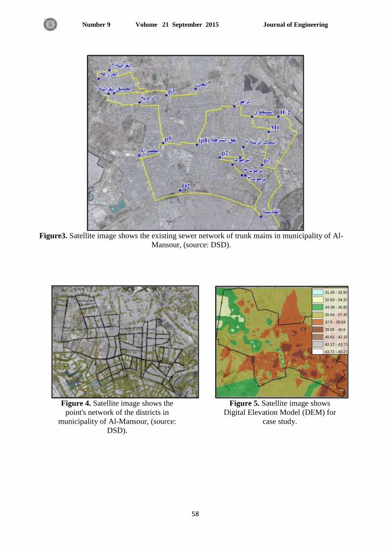
Journal of Engineering Volume 21 September 2015 Number 9
04
Figure3. Satellite image shows the existing sewer network of trunk mains in municipality of Al-
Mansour, (source: DSD).
Figure 4. Satellite image shows the
point's network of the districts in
municipality of Al-Mansour, (source:
DSD).
Figure 5. Satellite image shows
Digital Elevation Model (DEM) for
case study.
Legend
dman
<VALUE>
31.26 - 32.82
32.83 - 34.37
34.38 - 35.93
35.94 - 37.49
37.5 - 39.04
39.05 - 40.6
40.61 - 42.16
42.17 - 43.71
43.72 - 45.27

Journal of Engineering Volume 21 September 2015 Number 9
04
Figure 6. Complete streets network.
Figure 7. Command botton in the tool bar.
Figures 8. The minimum spanning streets network.

Journal of Engineering Volume 21 September 2015 Number 9
55
Figure 9. Project components after modification.
Figure 10. Larger scale of sample
section showing wet-well, pump,
and pressure pipes.
Figure 11. Schematic drawing
showing wet-well, pump, and
pressure pipes.
ma
Wet-well pump
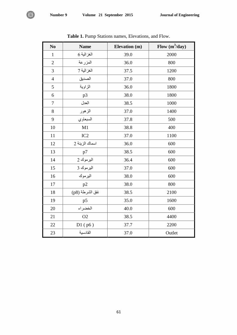
Journal of Engineering Volume 21 September 2015 Number 9
55
Table 1. Pump Stations names, Elevations, and Flow.
No Name Elevation (m) Flow (m3/day)
6 اغضا١ح 1 39.0 2000
800 36.0 اضسػح 2
4اغضا١ح 3 37.5 1200
800 37.0 اصذ٠ك 4
1800 36.0 اضا٠ح 5
6 p3 38.0 1800
1000 38.5 اؼذي 7
1400 37.0 اضس 8
500 37.8 اسثؼا 9
10 M1 38.8 400
11 IC2 37.0 1100
0اسان اض٠ح 12 36.0 600
13 p7 38.5 600
0 ١شنا 14 36.4 600
١3شن ا 15 37.0 600
600 38.0 ا١شن 16
17 p2 38.0 800
18 (p8) 2100 38.5 فك اششغح
19 p5 35.0 1600
600 40.0 اخعشاء 20
21 O2 38.5 4400
22 D1 ( p6 ) 37.7 2200
Outlet 37.0 امادس١ح 23

Journal of Engineering Volume 21 September 2015 Number 9
55
Table 2. Existing Trunk mains connecting Pump Stations.
No From sta. To sta. Length
(m) Sta
rt
dep
th
(m)
end
dep
th
(m)
Area (m2)
D.
(m) Vol. m
3
6اغضا١ح اضسػح 1 924.95 1.5 5.0 3006.09 0.50 1503.04
6اغضا١ح 2 P3 3953.76 2.0 6.0 15815.00 1.00 15815.04
374.80 0.50 749.59 4.0 1.5 272.58 اصذ٠ك 4اغضا١ح 3
Intersect 1598.66 1.5 6.0 5994.98 0.50 2997.49 اصذ٠ك 4
P5 2958.93 2.0 6.5 12575.50 1.00 12575.45 اضا٠ح 5
6 O2 19727.28 1.00 19727.30 7.0 2.0 4383.84 امادس١ح
P3 1680.82 1.5 7.0 7143.49 1.00 7143.49 اؼذي 7
٠3شن 8 557.40 1.00 557.40 4.0 1.0 222.96 ٠0شن
9 M1 P7 1715.00 1.5 6.5 6860.00 1.00 6860.00
10 اسان
اض٠حP6 839.44 1.5 4.5 2518.32 0.50 1259.16
11 P6 P2 1049.94 2.0 6.5 4462.25 1.00 4462.25
IC2 1344.82 1.5 5.5 4706.87 1.00 4706.87 اسثؼا 12
2635.80 0.50 5271.60 6.0 1.5 1405.76 اسثؼا اضس 13
14 P2 2889.25 1.00 2889.25 5.0 1.5 889.00 ٠شن
2343.71 0.75 3124.94 6.5 2.0 735.28 ٠3شن ٠شن 15
P8 3265.19 2.0 7.0 14693.40 1.00 14693.35 اضس 16
P5 1727.79 2.0 7 7775.06 1.00 7775.06 اخعشاء 17
M1 1808.23 1.5 6 6780.86 1.30 8815.12 اسثؼا 18
19 P7 Intersect 3906.17 2.0 7 17577.80 1.00 17577.77
٠0شن 20 10045.84 1.00 10045.80 6 2.0 2511.46 امادس١ح
21 IC2 Intersect 3622.53 2.0 7 16301.40 1.00 16301.39
22 P3 Intersect 1014.43 2.0 7 4564.94 1.00 4564.94
23 P5 P2 3173.72 1.5 6 11901.50 1.00 11901.45
24 P8 Intersect 306.18 2.0 7 1377.81 1.00 1377.81
Sum 44895.90 186421.00 178903.73
Unit cost (I.D.) 500,000
Total cost of excavation
(I.D.) 89,451,866,250

Journal of Engineering Volume 21 September 2015 Number 9
55
Table 3. UPVC Pipes Cost.
No. Dia. (m) Total Length
(m)
Price per unit
length (I.D.) Cost (I.D.)
1 0.50 5041 80,000 403,280,000
2 0.75 735 230,000 169,050,000
3 1.00 37726 400,000 15,090,000,000
4 1.30 1808 600,000 1,084,800,000
Total Cost 16,747,530,000
Table 4. Total Cost of existing sewer network.
Table 5. Minimum Streets lengths.
No From
sta. To sta. Length (m) No
From
sta. To sta. Length (m)
1 19 20 272.58 12 8 12 2715.78
2 20 10 1685.27 13 22 21 1344.70
3 11 23 1063.62 14 23 19 1173.03
4 17 10 2223.12 15 1 17 1711.96
5 6 5 1793.10 16 16 14 1731.50
6 5 4 1193.12 17 15 4 832.86
7 8 9 216.19 18 1 18 2790.74
8 2 8 745.501 19 7 3 1701.25
9 4 14 1302.44 20 22 16 1016.30
10 5 2 900.05 21 7 13 2678.52
11 7 6 1812.05 22 18 21 1390.45
Total length 32294.10
Item Cost in I.D.
Excavations Cost 89,451,866,250
Pipes Cost 16,747,530,000
Pump Stations Cost 69,000,000,000
Total Cost 175,199,396,250

Journal of Engineering Volume 21 September 2015 Number 9
58
Table 6. Result of Program Run.
No Pipe
Label
From
sta. To sta.
Length
(m)
Invert
Elv.
start (m)
Invert
Elv. stop
(m)
Start
depth
(m)
end
depth
(m)
Slope Area
(m2)
Dia.
(mm) Vol. m
3
1 swr-7 MH-2 MH-1 216.20 35.45 34.74 0.95 2.26 0.0033 347.00 254.00 88.14
2 swr-1 MH-3 W-16 272.60 36.34 35.84 1.16 1.16 0.0018 316.22 457.20 144.57
3 swr-17 MH-5 W-7 832.90 35.05 32.31 0.95 5.39 0.0033 2640.29 254.00 670.64
4 swr-3 MH-7 W-1 1063.60 37.92 34.92 1.08 1.08 0.0028 1148.69 304.80 350.12
5 swr-8 MH-9 MH-1 745.50 36.23 34.74 1.77 2.26 0.0020 1502.19 914.40 1373.60
6 swr-10 MH-10 W-19 900.00 36.23 35.33 1.77 2.67 0.0010 1998.00 914.40 1826.97
7 swr-20 MH-11 W-9 1016.30 35.39 34.37 1.61 4.43 0.0010 3069.23 762.00 2338.75
8 swr-14 MH-8 W-17 1173.00 34.84 33.49 1.16 4.01 0.0012 3032.21 457.20 1386.32
9 swr-6 MH-6 W-4 1193.10 36.09 34.89 1.61 3.11 0.0010 2815.72 914.40 2574.69
10 swr-22 MH-13 W-11 1390.40 35.54 34.15 1.46 3.65 0.0010 3552.47 762.00 2706.99
11 swr-9 MH-15 W-7 1302.40 36.89 32.31 1.61 5.39 0.0035 4558.40 762.00 3473.50
12 swr-5 MH-16 W-4 1793.10 37.04 34.89 1.46 3.11 0.0012 4097.23 609.60 2497.67
13 swr-13 MH-14 W-10 1344.70 36.34 34.99 1.46 2.01 0.0010 2333.05 762.00 1777.79
14 swr-19 MH-18 MH-17 1701.20 39.10 33.61 0.90 1.39 0.0032 1947.87 203.20 395.81
15 swr-2 MH-4 W-15 1685.30 35.69 34.01 1.31 1.99 0.0010 2780.75 533.40 1483.25
16 swr-4 MH-19 W-14 2223.10 34.69 32.47 1.31 5.53 0.0010 7603.00 609.60 4634.79
17 swr-15 MH-20 W-13 1712.00 36.54 34.83 1.46 3.67 0.0010 4391.28 609.60 2676.93
18 swr-16 MH-12 W-8 1731.50 37.19 35.45 1.61 3.05 0.0010 4034.40 762.00 3074.21
19 swr-11 MH-17 W-6 1812.00 33.61 31.80 1.39 6.70 0.0010 7329.54 609.60 4468.09
20 swr-18 MH-21 W-12 2790.70 37.04 34.25 1.46 2.75 0.0010 5874.42 762.00 4476.31
21 swr-12 MH-1 O-1 2715.80 34.74 32.02 2.26 4.98 0.0010 9831.20 1,066.80 10487.92
22 swr-21 MH-23 W-5 2678.50 37.27 33.77 1.23 1.23 0.0013 3294.56 457.20 1506.27
sum 32293.90 54413.32
Unit Cost 500,000
Total Cost 27,206,656,801

Journal of Engineering Volume 21 September 2015 Number 9
50
Table 7. UPVC pipes cost.
No Dia.
(mm)
Total
Length
unit
price Cost
1 203.20 1,701.20 50,000 85,060,000
2 254.00 1,049.00 60,000 62,940,000
3 304.80 1,063.60 70,000 74,452,000
4 457.20 4,124.10 80,000 329,928,000
5 533.40 1,685.30 120,000 202,236,000
6 609.60 7,540.20 180,000 1,357,236,000
7 762.00 9,576.10 230,000 2,202,480,000
8 914.40 2,838.70 400,000 1,135,480,000
9 1066.80 2,715.80 500,000 1,357,900,000
Total
Length 32,294.00
Total
Cost 6,807,735,000
Table 8. Overall Total cost of proposed sewer network.
Item Cost
Excavations Cost 19,510,900,000
Pipes Cost 6,807,735,000
Pump Stations Cost 69,000,000,000
Total Cost 95,318,635,000

Journal of Engineering Volume 21 September 2015 Number 9
55
Table 9. Cost comparison between existing network costs and proposed network costs.
Item Existing Network Proposed Network Reduction in
Cost
Excavations Cost 89,451,866,250 19,510,900,000 69,941,366,250
Pipes Cost 16,747,530,000 6,807,735,000 9,939,795,000
Pump Stations Cost 69,000,000,000 69,000,000,000 0
Total Cost 175,199,396,250 95,318,235,000 79,880,761,250


