Download - Hydrology principles ragunath


THIS PAGE ISBLANK


Copyright © 2006 New Age International (P) Ltd., PublishersPublished by New Age International (P) Ltd., Publishers
All rights reserved.
No part of this ebook may be reproduced in any form, by photostat, microfilm,xerography, or any other means, or incorporated into any information retrievalsystem, electronic or mechanical, without the written permission of the publisher.All inquiries should be emailed to [email protected]
ISBN (10) : 81-224-2332-9
ISBN (13) : 978-81-224-2332-7
PUBLISHING FOR ONE WORLD
NEW AGE INTERNATIONAL (P) LIMITED, PUBLISHERS4835/24, Ansari Road, Daryaganj, New Delhi - 110002Visit us at www.newagepublishers.com
C—9\N-HYDRO\HYD-TIT.PM5 IV
In this new Edition, two more Chapters are included, i.e.,
Chapter 17:Instantaneous Unit Hydrograph (IUH) with Clark and Nash Models illus-trated with Workedout Examples from field data.
Chapter 18:Cloud Seeding, the technique and operation being profusely illustrated withactual case histories in India and Russia.
Also, some more illustrative Field Examples are included under Infiltration, Storm Cor-relation, Gumbel’s and Regional Flood Frequency.
All, with a good print, sketches being neatly redrawn.
Comments are always welcome and will be incorporated in the succeeding editions.
H.M. Raghunath
PREFACE TO THE SECOND EDITION
( v )

THIS PAGE ISBLANK
C—9\N-HYDRO\HYD-TIT.PM5 V
Hydrology is a long continuing hydroscience and much work done in this field in the past,particularly in India, was of empirical nature related to development of empirical formulae,tables and curves for yield and flood of river basins applicable to the particular region in whichthey were evolved by investigators like Binnie, Barlow, Beale and Whiting, Strange, Ryves,Dicken, Inglis, Lacey, Kanwar Sain and Karpov, etc.
In this book, there is a departure from empiricism and the emphasis is on the collectionof data and analysis of the hydrological factors involved and promote hydrological design onsound principles and understanding of the science, for conservation and utilisation of waterresources. Hydrological designs may be made by deterministic, probabilistic and stochastic ap-proaches but what is more important is a ‘matured judgement’ to understand and avoid what istermed as ‘unusual meteorological combination’.
The book is written in a lucid style in the metric system of units and a large number ofhydrological design problems are worked out at the end of each article to illustrate the princi-ples of analysis and the design procedure. Problems for assignment are given at the end of eachChapter along with the objective type and intelligence questions. A list of references is includedat the end for supplementary reading. The book is profusely illustrated with sketches and is notbulky.
The text has been so brought to give confidence and competence for the reader to sit fora professional examination in the subject or enable him to take up independent field work as ahydrologist of a River basin or sub-basin.
The text is divided into Fundamental and Advanced topics and Appendices to fit thesemester-hours (duration) and the level at which the course is taught.
Degree and Post-degree students, research scholars and professionals in the fields ofCivil and Agricultural Engineering, Geology and Earth Sciences, find this book useful.
Suggestions for improving the book are always welcome and will be incorporated in thenext edition.
H.M. Raghunath
PREFACE TO THE FIRST EDITION
( vii )

THIS PAGE ISBLANK

Preface to the Second Edition (v)
Preface to the First Edition (vii)
����� ��������� ����� ���
1 Introduction 1
1.1 World’s Water Resources 31.2 Water Resources of India 31.3 Hydrological Study of Tapti Basin (Central India) 51.4 Hydrology and Hydrologic Cycle 111.5 Forms of Precipitation 131.6 Scope of Hydrology 141.7 Hydrological Data 141.8 Hydrologic Equation 15
2 Precipitation 17
2.1 Types of Precipitation 172.2 Measurement of Precipitation 182.3 Radars 222.4 Rain-gauge Density 222.5 Estimates of Missing Data and Adjustment of Records 232.6 Mean Areal Depth of Precipitation (Pave) 262.7 Optimum Rain-gauge Network Design 312.8 Depth-Area-Duration (DAD) Curves 332.9 Graphical Representation of Rainfall 362.10 Analysis of Rainfall Data 382.11 Mean and Median 432.12 Moving Averages Curve 482.13 Design Storm and PMP 492.14 Snow Pack and Snow Melt 49
3 Water Losses 60
3.1 Water Losses 603.2 Evaporation 60
CONTENTS

C—9\N-HYDRO\HYD-TIT.PM5 VII
3.3 Evaporation Pans 623.4 Soil Evaporation 663.5 Unsaturated Flow 663.6 Transpiration 673.7 Evapotranspiration 673.8 Hydrometeorology 703.9 Infiltration 703.10 Infiltration Indices 813.11 Supra Rain Technique 833.12 Watershed Leakage 873.13 Water Balance 87
4 Runoff 96
4.1 Components of Stream Flow 964.2 Catchment Characteristics 974.3 Mean and Median Elevation 1014.4 Classification of Streams 1034.5 Isochrones 1044.6 Factors Affecting Runoff 1044.7 Estimation of Runoff 106
5 Hydrographs 117
5.1 Hydrograph Components 1175.2 Separation of Streamflow Components 1205.3 Hydrograph Separation 1225.4 Unit Hydrograph 1245.5 Unit Hydrograph from Complex Storms 1305.6 S-Curve Method 1385.7 Bernard’s Distribution Graph 1425.8 Instantaneous Unit Hydrograph 1495.9 Synthetic Unit Hydrographs 1495.10 Transposing Unit Hydrographs 1545.11 Application of Unit Hydrograph 157
6 Stream Gauging 171
6.1 Methods of Measuring Stream Flow 1716.2 Current Meter Gaugings 1746.3 Stage-Discharge-Rating Curve 1786.4 Selection of Site for a Stream Gauging Station 183
7 Ground Water 192
7.1 Types of Aquifers and Formations 1927.2 Confined and Unconfined Aquifers 1937.3 Darcy’s Law 195
x CONTENTS
C—9\N-HYDRO\HYD-TIT.PM5 VIII
7.4 Transmissibility 1967.5 Well Hydraulics 1967.6 Specific Capacity 1997.7 Cavity Wells 2007.8 Hydraulics of Open Wells 2027.9 Construction of Open Wells 2067.10 Spacing of Wells 207
8 Floods-Estimation and Control 212
8.1 Size of Floods 2128.2 Estimation of Peak Flood 2138.4 Flood Frequency Studies 2218.5 Encounter Probability 2258.6 Methods of Flood Control 2388.7 Soil Conservation Measures 2458.8 Flood Control Economics 2478.9 Flood Forecasting and Warning 251
9 Flood Routing 262
9.1 Reservoir Routing 2629.2 Stream Flow Routing 270
10 Storage, Pondage and Flow Duration Curves 280
10.1 Reservoir Mass Curve and Storage 28010.2 Flow Duration Curves 28510.3 Pondage 288
11 Reservoir Sedimentation 298
11.1 Sediment Movement and Deposition 29811.2 Reduction in Reservoir Capacity 30011.3 Reservoir Sedimentation Control 303
12 Arid, Semi-Arid and Humid Regions 306
12.1 Arid Regions 30612.2 Semi-Arid Regions 30712.3 Humid Regions 309
������������� ������
13 Linear Regression 315
13.1 Fitting Regression Equation 31513.2 Standard Error of Estimate 31613.3 Linear Multiple Regression 31913.4 Coaxial Graphical Correlation of Rainfall Runoff 322
CONTENTS xi

C—9\N-HYDRO\HYD-TIT.PM5 IX
14 Statistical and Probability Analysis of Hydrological Data 327
14.1 Elements of Statistics 32714.2 Probability of Hydrologic Events 332
15 Flood Frequency—Probability and Stochastic Methods 337
15.1 Flood Frequency Methods 33715.2 Stochastic Method 34415.3 Stochastic Modelling by the Partial Duration Series 34415.4 Annual Flood Peaks—River Ganga 35815.5 Regional Flood-Frequency Analysis (RFFA) 361
16 Mathematical Models in Hydrology 366
16.1 Type of Mathematical Models 36616.2 Methods of Determining IUH 37116.3 Synthetic Stream Flow 37916.4 Flow at Ungauged Sites by Multiple Regression 38116.5 Reservoir Mass Curve 38116.6 Residual Mass Curve 38316.7 Selection of Reservoir Capacity 38316.8 Flood Forecasting 38616.8 Mathematical Model 389
17 Instantaneous Unit Hydrograph (IUH) 393
17.1 IUH for a Basin 39317.2 Derivation of IUH 39317.3 Other Methods of Derivation of IUH 39417.4 NASH Conceptual Model 39417.5 Clark’s Model 39717.6 Drawing Isochrones and Time-Area Diagram (TAD) 39817.7 Clark’s Method 398
18 Cloud Seeding 403
18.1 Conditions for Cloud Seeding 40318.2 Cloud Seeding Technique 40418.3 Cloud Seeding Operation 40618.4 Recent Case History 406
Appendices 407
Selected References 453
Bibliography 456
Index 457
xii CONTENTS
PART A
FUNDAMENTAL HYDROLOGY

THIS PAGE ISBLANK

Chapter 1
Hydrology is a branch of Earth Science. The importance of hydrology in the assessment,development, utilisation and management of the water resources, of any region is being in-creasingly realised at all levels. It was in view of this that the United Nations proclaimed theperiod of 1965-1974 as the International Hydrological Decade during which, intensive effortsin hydrologic education research, development of analytical techniques and collection of hy-drological information on a global basis, were promoted in Universities, Research Institutions,and Government Organisations.
1.1 WORLD’S WATER RESOURCES
The World’s total water resources are estimated at 1.36 × 10⁸ Μ ha-m. Of these global waterresources, about 97.2% is salt water mainly in oceans, and only 2.8% is available as freshwater at any time on the planet earth. Out of this 2.8% of fresh water, about 2.2% is availableas surface water and 0.6% as ground water. Even out of this 2.2% of surface water, 2.15% isfresh water in glaciers and icecaps and only of the order of 0.01% is available in lakes andstreams, the remaining 0.04% being in other forms. Out of 0.6% of stored ground water, onlyabout 0.25% can be economically extracted with the present drilling technology (the remain-ing being at greater depths). It can be said that the ground water potential of the Ganga Basinis roughly about forty times the flow of water in the river Ganga.
1.2 WATER RESOURCES OF INDIA
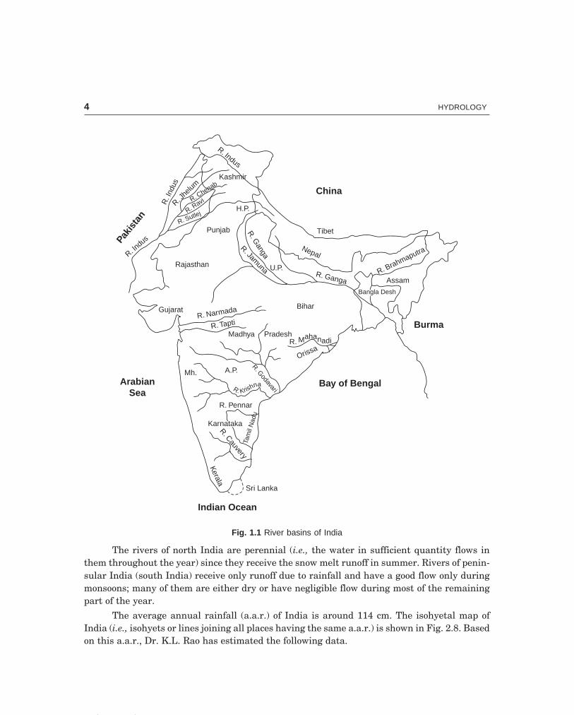
The important rivers of India are shown in Fig. 1.1 and their approximate water potentials aregiven below:
Water potentialSl. no. River basin
(M ha-m)
1. West flowing rivers like Narmada and Tapti 30.55
2. East flowing rivers like Mahanadi, Godavari,Krishna, Cauvery and Pennar 35.56
3. The Ganges and its tributaries 55.01
4. Indus and its tributaries 7.95
5. The River Brahmaputra 59.07
Total 188.14
INTRODUCTION
3
C-9\N-HYDRO\HYD1-1.PM5 4
4 HYDROLOGY
R. Indus
Kashmir
R. RaviR. J
helum
R. Chenab
R. SutlejH.P.
Punjab
R. I
ndus
China
Tibet
Nepal
R. G
anga
U.P.
R. Jamuna
R. Ganga
RajasthanR. In
dusPaki
stan
GujaratR. Narmada
R. Tapti
Bihar
Madhya PradeshR. Mahanadi
Orissa
R. GodavariR. Krishna
Mh. A.P.
R. Pennar
KarnatakaKarnataka
Tam
ilN
adu
R. Cauvery
Kerala
Sri Lanka
Indian Ocean
ArabianSea
Bay of Bengal
Burma
Bangla DeshBangla Desh
AssamR. Brahmaputra
Fig. 1.1 River basins of India
The rivers of north India are perennial (i.e., the water in sufficient quantity flows inthem throughout the year) since they receive the snow melt runoff in summer. Rivers of penin-sular India (south India) receive only runoff due to rainfall and have a good flow only duringmonsoons; many of them are either dry or have negligible flow during most of the remainingpart of the year.
The average annual rainfall (a.a.r.) of India is around 114 cm. The isohyetal map ofIndia (i.e., isohyets or lines joining all places having the same a.a.r.) is shown in Fig. 2.8. Basedon this a.a.r., Dr. K.L. Rao has estimated the following data.

C-9\N-HYDRO\HYD1-1.PM5 5
INTRODUCTION 5
Sl. no. Item Approximate volume(M ha-m)
1. Annual rainfall over the entire country 370
2. Evaporation loss @ 13 of item (1) above 123
3. Runoff (from rainfall) in rivers 167
4. Seepage into subsoil by balance (1)—{(2) + (3)} 80
5. Water absorbed in top soil layers, i.e., contributionto soil moisture 43
6. Recharge into ground water (from rainfall) (4)—(5) 37
7. Annual ground water recharge from rainfall and seepagefrom canals and irrigation systems (approximate) 45
8. Ground water that can be economically extracted fromthe present drilling technology @ 60% of item (7) 27
9. Present utilisation of ground water @ 50% of item (8) 13.5
10. Available ground water for further exploitation andutilisation 13.5
The geographical area of the country (India) is 3.28 Mkm2 and the annual runoff(from rainfall) is 167 M ha-m (or 167 × 104 Mm3), which is approximately two-and half-timesof the Mississippi-Missouri river Basin, which is almost equal in area to the whole of India.Due to limitations of terrain, non-availability of suitable storage sites, short period of occur-rence of rains, etc. the surface water resources that can be utilised has been estimated asonly 67 M ha-m. The total arable land in India is estimated to be 1.47 Mkm2 which is 45%of the total geographical area against 10% for USSR and 25% for USA. India has a greatpotential for agriculture and water resources utilisation. A case history of the ‘Flood Hydrol-ogy of Tapti Basin’ is given below for illustration.
1.3 HYDROLOGICAL STUDY OF TAPTI BASIN (CENTRAL INDIA)
Tapti is one of the two large rivers in central India which flows west-ward (the other one beingriver Narmada) and discharge into the Arabian Sea. Tapti takes its origin in Multai Hills inthe Gavilgadh hill ranges of Satpura mountain in Madhya Pradesh, Fig. 1.2. Tapti is the mostsignificant flood-menacing river as far as the state of Gujarat is concerned.
The River Tapti is 720 km long and runs generally to west through Madhya Pradesh(208 km), Maharashtra (323 km) and Gujarat (189 km) states joining the Arabian Sea in theGulf of Cambay approximately 20 km west of the city of Surat. The river course according tothe topographical features of its run can be divided into four sections as follows:

C-9\N-HYDRO\HYD1-1.PM5 6
6 HYDROLOGY
Fig
. 1.
2 Ta
pti b
asin
22°
21°
20°
22°
21°
20°
73°
74°
75°
76°
77°
78°
73°
74°
75°
76°
77°
78°N
Mul
tai
Tal
ega
on
Bas
inbo
unda
ry
Ako
la
R. P
urna
R.T
api
Bur
hanp
ur
Mad
hya
Pra
desh
Mah
aras
htra
Bhu
saw
alJa
lga
-on
Nan
ded
R.Yaghur
Cha
lisga
on
R.G
irna
Shi
rpur
Sha
had
R.G
omai
Mah
aras
htra
R.B
uray
R. P
anjh
ra Dhu
lia R.B
ori
Mal
egao
n
Riv
erT
api
Kak
rapa
rw
eir K
adod
Uka
iS
urat
Guj
arat
Gul
fof
Cam
bay
ArabianSea
Bas
inch
arac
teris
tics
A=
6220
0km
L=
720
km(t
halw
eg)
2
b W=
86.5
kmb
=
P=
1840
kmC
ompa
ctne
ssC
oeffi
cien
t =2.
08
For
mfa
ctor
==
0.12
km20
1010
20km
0S
cale
A L b
L bWb
R.A
nar

C-9\N-HYDRO\HYD1-1.PM5 7
INTRODUCTION 7
The catchment areas of the river Tapti above Burhanpur and Bhusaval are 81800 and31350 km2, respectively. The catchment area of the river before it enters the Gujarat state isabout 57000 km2, while the catchment at Surat is 61800 km2. Thus, most of the catchment canbe called hilly with good gradients. The important tributaries, their catchment areas and thelength of their run are given below:
Tributary Catchment River at confluencearea (km2) (km)
Purna 17920 282
Waghur 2352 312
Girna 9720 340
Bori 2344 386
Anar 1350 382
Panjhra 2860 400
Buray 1038 424
Gomai 1263 481
1. Section I II III IV
2. Length (km) 240 288 80 112
3. Terrain Dense forests;hill ranges hugthe river banks,Rocky bed andsteep banks asthe riverpasses throughSatpura moun-tain ranges
Several largetributaries joinon both sides.Rich fertileplains of east andwest Khandeshdistricts ofMaharastra
Hilly tract cov-ered with for-ests, Number ofrapids betweenKamalapur andKakrapur a dis-tance of 32 km.At Kakrapur theriver falls by7.5 m; beyondKakrapur theriver widens toabout 900 m
Low flat alluvialplains of Gujarat.River meanderspast towns ofKathor and Surat.Numerous rapidsnear towns ofMandvi and Kadod
4. Catchmentarea (km2)
1000 (aboveBurhanpur)
15000
5. Average bed slopein the reach (m/km)
2.16 0.52 0.56 0.35
6. a.a.r. (cm) 75-150 50-75 (heavyrainfall in Ghatcatchment ofGirna river≈ 150 cm)
150 100-150
C-9\N-HYDRO\HYD1-1.PM5 8
8 HYDROLOGY
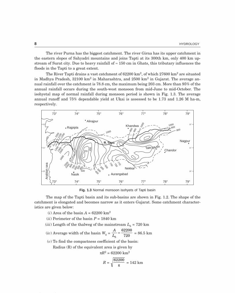
The river Purna has the biggest catchment. The river Girna has its upper catchment inthe eastern slopes of Sahyadri mountains and joins Tapti at its 300th km, only 400 km up-stream of Surat city. Due to heavy rainfall of ≈ 150 cm in Ghats, this tributary influences thefloods in the Tapti to a great extent.
The River Tapti drains a vast catchment of 62200 km2, of which 27600 km2 are situatedin Madhya Pradesh, 32100 km2 in Maharashtra, and 2500 km2 in Gujarat. The average an-nual rainfall over the catchment is 78.8 cm, the maximum being 203 cm. More than 95% of theannual rainfall occurs during the south-west monsoon from mid-June to mid-October. Theisohyetal map of normal rainfall during monsoon period is shown in Fig. 1.3. The averageannual runoff and 75% dependable yield at Ukai is assessed to be 1.73 and 1.26 M ha-m,respectively.
22°
21°
20°
22°
21°
20°
73° 74° 75° 76° 77° 78° 79°
73° 74° 75° 76° 77° 78° 79°
Alirajpur
Rajpipla
1000
1100
1200
1300
1400
1500
1600
1500
1000 800
700
650
500
450
500
Ara
bian
sea
Nasik Aurangabad
Nekkar450
500
650
500
730750
770
1000
450
431
Khandwa80
090
0
1000
Tale ga onChandor
Nagpur
1000900
800
R.Tapti
Fig. 1.3 Normal monsoon isohyets of Tapti basin
The map of the Tapti basin and its sub-basins are shown in Fig. 1.2. The shape of thecatchment is elongated and becomes narrow as it enters Gujarat. Some catchment character-istics are given below:
(i) Area of the basin A = 62200 km2
(ii) Perimeter of the basin P = 1840 km(iii) Length of the thalweg of the mainstream Lb = 720 km
(iv) Average width of the basin Wb = ALb
=62200
720 = 86.5 km
(v) To find the compactness coefficient of the basin:Radius (R) of the equivalent area is given by
πR2 = 62200 km2
R = 62200
π = 142 km

C-9\N-HYDRO\HYD1-1.PM5 9
INTRODUCTION 9
Circumference of the equivalent circular area= 2πR = 2π × 142 = 886 km
Compactness coefficient of the basin
= PR2
1840886π
= = 2.08
(vi) From factor Ff = WL
AL
b
b b
= =2 2
62200720
= 0.12
Sometimes, the reciprocal of this taken as the coefficient of shape of the basin (= 8.3).
(vii) Elongation ratio Er = 2 2 142
720R
Lb= ×
= 0.4
Narmada and Tapti catchments, which are adjacent are often hit by storms caused bydepression originating both from the Arabian Sea and the Bay of Bengal, which cause heavyrains resulting in high floods. The tracks of the monsoon depressions that caused heavy rains*(25.96 cm) during August 4-6, 1968 are shown in Fig. 1.4. The Tapti catchment being not di-rectly affected by the tracks of these storms but falling in the south-westen sector of storms,
30°
25°
20°
15°
10°
65° 70° 75° 80° 85° 90°
6 5 4
3 2
1Tapticatchment
Storm trackNarmadacatchment
Bay ofBengal
Arabiansea
7
Fig. 1.4 Storm track of August 1968
gets a well-distributed rainfall over its entire catchment except its extreme western end, wherea steep isohyetal gradient exists due to the influence of the western Ghats. Many times thedepressions move along the river courses synchronising with the movement of floods. Thisphenomenon causes devastating floods. The river widens out at the lower reach. Low tidescome as far as Surat and high tides travel very much upstream. Many times high tides andtidal waves due to storms, synchronise with floods resulting in devastation. Particularly nearthe Gulf, the water becomes a vast sheet of water extending from Narmada to Mindhola, a
*The highest flood peak of R. Tapti in 1968 was 42,500 cumec, while of R. Narmada was 58,000 cumecin 1968 and 69,400 cumec in 1970.

C-9\N-HYDRO\HYD1-1.PM5 10
10 HYDROLOGY
distance of about 72 km. Therefore a proper flood warning system and raised platforms wouldbe necessary. The city of Surat lies between elevations +21 and +32 m. The river spills over itsbanks at two places above Surat, i.e., at Dholanpardi above the National Highway andNanavaracha. These spills are obstructed by high embankments of railways, roads and canalscausing interruptions in these services and damages to lands and property due to inundationof floods. The city of Surat and the surrounding fertile delta are quite low and are vulnerableto floods.
The highest ever flood seems to have occurred in 1837; most of the heavy floods haveoccurred in August and September. The recent high floods in 1959 and 1968 were catastrophicand brought untold damages to industry, commerce and normal life of the city of Surat. Anassessment of the damages caused by these floods are given below.
Sl. Flood in No. of villages Human Cattle Damage to Houses damagedno. the year affected casualty loss standing or destroyed
crops (ha.)
1. 1959 194 79 554 30460 14815
2. 1968 505 112 7649 38540 30606
The ‘depth-duration’ and the ‘depth-area-duration’ curves for the heavy storms duringAugust 4-6, 1968 (3 days) are shown in Fig. 1.5 and Fig. 2.15. The weighted maximum rainfalldepth for the Tapti basin up to Ukai for 1, 2, and 3 days are 11.43, 22.38, and 25.96 cm,respectively.
The maximum representative dew point of Tapti basin during the storm period (Aug 4-6,1968), after reducing to the reference level of 1000 mb, was 29.8 °C and the persisting repre-sentative dew point for the storm was 26.7 °C. The moisture adjustment factor (MAF), which isthe ratio of maximum precipitable water at the storm location to the precipitable water availableduring the storm period, was derived with respect to the standard level of 500 mb (by refer-ence to the diagram given by Robert D. Fletcher of US Weather Bureau as
MAF = Depth of maximum precipitable water (1000 mb to 500 mb)
Depth of storm precipitable water (1000 mb to 500 mb)
= 98 mm80 mm
= 1.23
The storm of August 4-6, 1968 was ‘increased by 23% to arrive at the maximum prob-able storm (MPS) of 31.8 cm, assuming the same mechanical efficiency. This MPS with mini-mum infiltration losses and the rainfall excesses (net rainfall or runoff) rearranged duringsuccessive 6-hour intervals, was applied to the ordinates of the 6-hour design unit hydrograph(derived from the 1968 flood hydrograph at Kakrapar weir at Ukai) to obtain the design floodhydrograph, the peak of which gave the maximum probable flood (MPF) of 59800 cumec (seeexample 8.4). The highest flood peak observed during 1876-1968 (93 years) was 42500 cumecin August 1968 (Fig. 1.6). The standard project flood (SPF) recommended by the Central Wa-ter and Power Commission (CWPC), New Delhi for the design of Ukai dam was around 48200cumec and the design flood adopted was 49500 cumec. The MPF recommended by CWPC wasalso 59800 cumec.

C-9\N-HYDRO\HYD1-1.PM5 11
INTRODUCTION 11
1 2 3(Days)
25
20
15
10
5
0
Rai
nfal
ldep
th,(
cm)
Aug 1968
July 1941Sept 1945Sept 1904July 1894Sept 1959Aug 1944
July 1896
Sept 1949
Sept 1891Sept 1954Aug 1958
Fig. 1.5 Depth-duration curves for heavy-rain storms of Tapti basin
For the 3-day storm of 1968, the rainfall of 25.96 cm has resulted in a surface runoff of
11.68 cm, thus giving a coefficient of runoff of 11.6825 96.
= 0.43 for the whole catchment. During
this flood, there was a wind storm of 80 km/hr blowing over the city of Surat. There wassimultaneous high tide in the river. There was heavy storm concentration in the lower catch-ment. The total loss due to the devastating floods of 1968 was around Rs. 100 lakhs.
In Chapter 15, the magnitudes and return periods (recurrence intervals) of the highfloods are determined by the deterministic, probabilistic and stochastic approaches using theannual flood data of the lower Tapti river at Ukai for the 30-years period from 1939 to 1968.The Gumbel’s method, based on the theory of extreme values gives a 100-year flood of 49210cumec and hence this method can be safely adopted in the estimation of design flood for thepurpose of safe design of hydraulic structures, while the stochastic approach may give a suit-able value of MPF.
1.4 HYDROLOGY AND HYDROLOGIC CYCLE
Hydrology is the science, which deals with the occurrence, distribution and disposal of wateron the planet earth; it is the science which deals with the various phases of the hydrologiccycle.

C-9\N-HYDRO\HYD1-1.PM5 12
12 HYDROLOGY
50
45
40
35
30
25
20
15
10
5
00 20 40 60 80 100 120 140 160 180
Time (hr)
Dis
char
geQ
(100
0cu
mec
)
49500 cumec
42500 cumec (1968 flood)
37300 cumec (1959 flood)
Observed floodhydrographs (1968 & 1959)
Design flood hydrograph
25
20
15
10
5
00 5 10 15 20 25 30 35 40 45 50 55 60
Discharge (1000 cumec)
Rai
nfal
l,(c
m)
Rainfall-runoff curve
Fig. 1.6 Flood hydrographs of river Tapti at Ukai
Hydrologic cycle is the water transfer cycle, which occurs continuously in nature; thethree important phases of the hydrologic cycle are: (a) Evaporation and evapotranspiration (b)precipitation and (c) runoff and is shown in Fig. 1.7. The globe has one-third land and two-thirds ocean. Evaporation from the surfaces of ponds, lakes, reservoirs. ocean surfaces, etc.and transpiration from surface vegetation i.e., from plant leaves of cropped land and forests,etc. take place. These vapours rise to the sky and are condensed at higher altitudes by conden-sation nuclei and form clouds, resulting in droplet growth. The clouds melt and sometimesburst resulting in precipitation of different forms like rain, snow, hail, sleet, mist, dew andfrost. A part of this precipitation flows over the land called runoff and part infilters into thesoil which builds up the ground water table. The surface runoff joins the streams and thewater is stored in reservoirs. A portion of surface runoff and ground water flows back to ocean.Again evaporation starts from the surfaces of lakes, reservoirs and ocean, and the cycle re-peats. Of these three phases of the hydrologic cycle, namely, evaporation, precipitation and
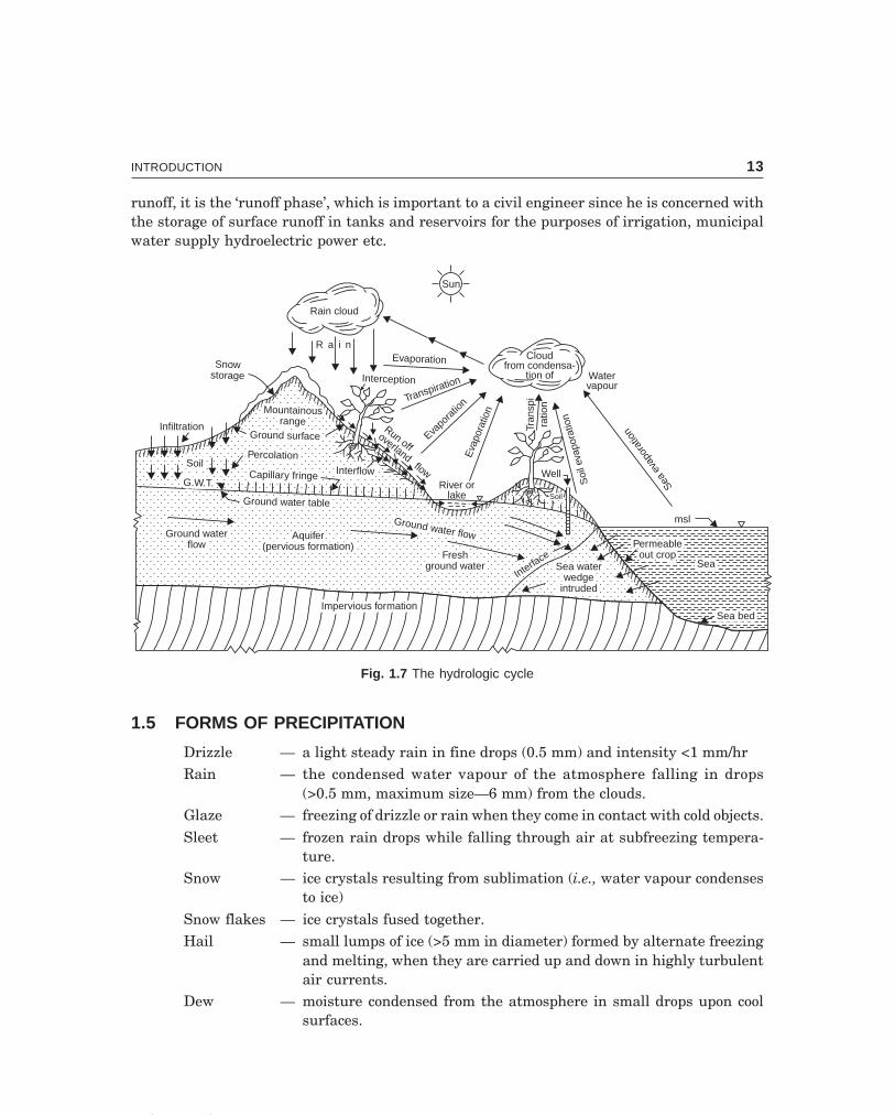
C-9\N-HYDRO\HYD1-1.PM5 13
INTRODUCTION 13
runoff, it is the ‘runoff phase’, which is important to a civil engineer since he is concerned withthe storage of surface runoff in tanks and reservoirs for the purposes of irrigation, municipalwater supply hydroelectric power etc.
msl
Sea waterwedge
intruded
Sea waterwedge
intruded
SeaSea
Permeableout crop
Permeableout crop
Sea bedSea bed
Freshground water
Freshground water
Ground water flowGround water flowAquifer
(pervious formation)Aquifer
(pervious formation)Ground water
flowGround water
flow
Ground water tableGround water table
Interface
Interface
Impervious formationImpervious formation
G.W.T.G.W.T.
Infiltration
SoilSoilCapillary fringeCapillary fringe
PercolationPercolation
Ground surfaceGround surface
Mountainousrange
Mountainousrange
Snowstorage
InterflowInterflow Well
SoilSoil
Rain cloud
R a i nEvaporation
Transpiration
Evapo
ratio
n
Eva
pora
tion
Interception
Run offoverland
flowRiver or
lake
Cloudfrom condensa-
tion of Watervapour
Sea
evap
orat
ion
Soi
leva
pora
tion
Tran
spi
ratio
n
Sun
Fig. 1.7 The hydrologic cycle
1.5 FORMS OF PRECIPITATION
Drizzle — a light steady rain in fine drops (0.5 mm) and intensity <1 mm/hrRain — the condensed water vapour of the atmosphere falling in drops
(>0.5 mm, maximum size—6 mm) from the clouds.Glaze — freezing of drizzle or rain when they come in contact with cold objects.Sleet — frozen rain drops while falling through air at subfreezing tempera-
ture.Snow — ice crystals resulting from sublimation (i.e., water vapour condenses
to ice)Snow flakes — ice crystals fused together.Hail — small lumps of ice (>5 mm in diameter) formed by alternate freezing
and melting, when they are carried up and down in highly turbulentair currents.
Dew — moisture condensed from the atmosphere in small drops upon coolsurfaces.

C-9\N-HYDRO\HYD1-1.PM5 14
14 HYDROLOGY
Frost — a feathery deposit of ice formed on the ground or on the surface ofexposed objects by dew or water vapour that has frozen
Fog — a thin cloud of varying size formed at the surface of the earth bycondensation of atmospheric vapour (interfering with visibility)
Mist — a very thin fog
1.6 SCOPE OF HYDROLOGY
The study of hydrology helps us to know(i) the maximum probable flood that may occur at a given site and its frequency; this is
required for the safe design of drains and culverts, dams and reservoirs, channelsand other flood control structures.
(ii) the water yield from a basin—its occurence, quantity and frequency, etc; this isnecessary for the design of dams, municipal water supply, water power, river navi-gation, etc.
(iii) the ground water development for which a knowledge of the hydrogeology of thearea, i.e., of the formation soil, recharge facilities like streams and reservoirs, rain-fall pattern, climate, cropping pattern, etc. are required.
(iv) the maximum intensity of storm and its frequency for the design of a drainage projectin the area.
1.7 HYDROLOGICAL DATA
For the analysis and design of any hydrologic project adequate data and length of records arenecessary. A hydrologist is often posed with lack of adequate data. The basic hydrological datarequired are:
(i) Climatological data(ii) Hydrometeorological data like temperature, wind velocity, humidity, etc.
(iii) Precipitation records(iv) Stream-flow records(v) Seasonal fluctuation of ground water table or piezometric heads
(vi) Evaporation data(vii) Cropping pattern, crops and their consumptive use
(viii) Water quality data of surface streams and ground water(ix) Geomorphologic studies of the basin, like area, shape and slope of the basin, mean
and median elevation, mean temperature (as well as highest and lowest tempera-ture recorded) and other physiographic characteristics of the basin; stream densityand drainage density; tanks and reservoirs
(x) Hydrometeorological characteristics of basin:(i) a.a.r., long term precipitation, space average over the basin using isohyets and
several other methods (Rainbird, 1968)(ii) Depth-area-duration (DAD) curves for critical storms (station equipped with
self-recording raingauges).

C-9\N-HYDRO\HYD1-1.PM5 15
INTRODUCTION 15
(iii) Isohyetal maps—Isohyets may be drawn for long-term average, annual andmonthly precipitation for individual years and months
(iv) Cropping pattern—crops and their seasons(v) Daily, monthly and annual evaporation from water surfaces in the basin
(vi) Water balance studies of the basin(vii) Chronic problems in the basin due to a flood-menacing river (like Tapti or Tapi
in central India) or siltmenacing river (like Tungabhadra in Karnataka)(vii) Soil conservation and methods of flood control
1.8 HYDROLOGIC EQUATION
The hydrologic equation is simply the statement of the law of conservation of matter and isgiven by
I = O + ∆S ...(1.1)where I = inflow
O = outflow ∆S = change in storage
This equation states that during a given period, the total inflow into a given area mustequal the total outflow from the area plus the change is storage. While solving this equation,the ground water is considered as an integral part of the surface water and it is the subsurfaceinflow and outflow that pose problems in the water balance studies of a basin.
������
I Choose the correct statement/s in the following:
1 The hydrological cycle
(i) has beginning but does not end
(ii) has both beginning and end
(iii) occurs continuously in nature
(iv) is a water transfer cycle
(v) has three phases—precipitation, evaporation and runoff
2 Hydrology deals with
(i) occurrence of water and formation of snow
(ii) movement of water on earth and water vapour in atmosphere
(iii) occurrence of floods and droughts
(iv) consumptive use of crops and crop planning
(v) prevention of drought
(iv) the hydrologic cycle
3 Hydrologic studies are made
(i) to determine MPF
(ii) to determine design flood for spillways and bridges
(iii) to asses the ground water potential of a basin
C-9\N-HYDRO\HYD1-1.PM5 16
16 HYDROLOGY
(iv) for the preparation of land drainage schemes
(v) to determine the hydro-power potential
(iv) for irrigation and crop planning
(vii) for all the above
4 The hydrologic equation states that
(i) the inflow into the basin is equal to the outflow from the basin at any instant
(ii) the difference between inflow and outflow is the storage
(iii) subsurface inflow is equal to the subsurface outflow
(iv) the water balance over the basin = Σ inflow — Σ outflow
II Match the items in ‘A’ with items in ‘B’
A B(i) Runoff (a) Deals with hydrologic cycle
(ii) Snow, hail (b) Water transfer cycle
(iii) Hydrology (c) Important phase of hydrologic cycle
(iv) Hydrologic cycle (d) Forms of precipitation
(v) Evaporation, precipitation and runoff (e) Law of conservation of matter
(vi) Hydrologic equation (f) Three phases of hydrologic cycle
�������
1 Explain the hydraulic cycle in nature with the help of a neat sketch, indicating its various phases.
2 What are the basic data required for hydrological studies? Name the agencies from which thedata can be obtained?
3 What is the function of hydrology in water resources development? What are the basic hydrologicalrequirements for a river basin development?
4 Explain ‘hydrologic equation’.

Chapter 2
The precipitation in the country (India) is mainly in the form of rain fall though there isappreciable snowfall at high altitudes in the Himalayan range and most of the rivers in northIndia are perennial since they receive snow-melt in summer (when there is no rainfall).
2.1 TYPES OF PRECIPITATION
The precipitation may be due to(i) Thermal convection (convectional precipitation)—This type of precipiation is in the
form of local whirling thunder storms and is typical of the tropics. The air close to the warmearth gets heated and rises due to its low density, cools adiabatically to form a cauliflowershaped cloud, which finally bursts into a thunder storm. When accompanied by destructivewinds, they are called ‘tornados’.
(ii) Conflict between two air masses (frontal precipitation)—When two air masses dueto contrasting temperatures and densities clash with each other, condensation and precipita-tion occur at the surface of contact, Fig. 2.1. This surface of contact is called a ‘front’ or ‘frontalsurface’. If a cold air mass drives out a warm air mass’ it is called a ‘cold front’ and if a warm airmass replaces the retreating cold air mass, it is called a ‘warm front’. On the other hand, if thetwo air masses are drawn simultaneously towards a low pressure area, the front developed isstationary and is called a ‘stationary front’. Cold front causes intense precipitation on com-paratively small areas, while the precipitation due to warm front is less intense but is spreadover a comparatively larger area. Cold fronts move faster than warm fronts and usually over-take them, the frontal surfaces of cold and warm air sliding against each other. This phenom-enon is called ‘occlusion’ and the resulting frontal surface is called an ‘occluded front’.
(ii) Orographic lifting (orographic precipitation)—The mechanical lifting of moist airover mountain barriers, causes heavy precipitation on the windward side (Fig. 2.2). For exam-ple Cherrapunji in the Himalayan range and Agumbe in the western Ghats of south India getvery heavy orographic precipitation of 1250 cm and 900 cm (average annual rainfall), respec-tively.
(iv) Cyclonic (cyclonic precipitation)—This type of precipitation is due to lifting of moistair converging into a low pressure belt, i.e., due to pressure differences created by the unequalheating of the earth’s surface. Here the winds blow spirally inward counterclockwise in thenorthern hemisphere and clockwise in the southern hemisphere. There are two main types ofcyclones—tropical cyclone (also called hurricane or typhoon) of comparatively small diameterof 300-1500 km causing high wind velocity and heavy precipitation, and the extra-tropicalcyclone of large diameter up to 3000 km causing wide spread frontal type precipitation.
17
PRECIPITATION

C-9\N-HYDRO\HYD2-1.PM5 18
18 HYDROLOGY
Frontal surfacecold air mass Warm air
mass
(a) Cold front (b) Warm front
Cold airmass
Frontal surface
Warm airmass
Warmair
Cold airColder air
(c) Stationary front
Low pressure
Fig. 2.1 Frontal precipitation
Sea
msl
Heavy rain
Windward(Seaward side)
Mountainousrange
Leeward(Landward) side
Rain-shadow area
Land
Fig. 2.2 Orographic precipitation
2.2 MEASUREMENT OF PRECIPITATION
Rainfall may be measured by a network of rain gauges which may either be of non-recording orrecording type.
50
Measuringjar (glass)
60 cm60 cm
20 cm20 cm
55 cm55 cm
25 cm25 cm
5 cmGL 5 cm5 cm
GL
Masonryfoundation block
60 cm × 60 cm × 60 cm
12.5 cm
Rim (30 cm above GL)
Metal casing
Funnel
Glass bottle(7.5-10 cm dia.)
Ground level
Fig. 2.3 Symon’s rain gauge

C-9\N-HYDRO\HYD2-1.PM5 19
PRECIPITATION 19
The non-recording rain gauge used in India is the Symon’s rain gauge (Fig. 2.3). It con-sists of a funnel with a circular rim of 12.7 cm diameter and a glass bottle as a receiver. Thecylindrical metal casing is fixed vertically to the masonry foundation with the level rim 30.5cm above the ground surface. The rain falling into the funnel is collected in the receiver and ismeasured in a special measuring glass graduated in mm of rainfall; when full it can measure1.25 cm of rain.
The rainfall is measured every day at 08.30 hours IST. During heavy rains, it must bemeasured three or four times in the day, lest the receiver fill and overflow, but the last meas-urement should be at 08.30 hours IST and the sum total of all the measurements during theprevious 24 hours entered as the rainfall of the day in the register. Usually, rainfall measure-ments are made at 08.30 hr IST and sometimes at 17.30 hr IST also. Thus the non-recording orthe Symon’s rain gauge gives only the total depth of rainfall for the previous 24 hours (i.e.,daily rainfall) and does not give the intensity and duration of rainfall during different timeintervals of the day.
It is often desirable to protect the gauge from being damaged by cattle and for thispurpose a barbed wire fence may be erected around it.
Recording Rain GaugeThis is also called self-recording, automatic or integrating rain gauge. This type of rain gaugeFigs. 2.4, 2.5 and 2.6, has an automatic mechanical arrangement consisting of a clockwork, adrum with a graph paper fixed around it and a pencil point, which draws the mass curve ofrainfall Fig. 2.7. From this mass curve, the depth of rainfall in a given time, the rate or inten-sity of rainfall at any instant during a storm, time of onset and cessation of rainfall, can bedetermined. The gauge is installed on a concrete or masonry platform 45 cm square in theobservatory enclosure by the side of the ordinary rain gauge at a distance of 2-3 m from it. Thegauge is so installed that the rim of the funnel is horizontal and at a height of exactly 75 cmabove ground surface. The self-recording rain gauge is generally used in conjunction with anordinary rain gauge exposed close by, for use as standard, by means of which the readings ofthe recording rain gauge can be checked and if necessary adjusted.
30 cm
Receiver
FunnelTipping bucket
To recordingdevice
Measuring tube
Revolving drum(chart mounted)
Clock mechanism Pen
Springbalance
Catchbucket
Metal cover
Receivingfunnel
Fig. 2.4 Tipping bucket gauge Fig. 2.5 Weighing type rain gauge

C-9\N-HYDRO\HYD2-1.PM5 20
20 HYDROLOGY
There are three types of recording rain gauges—tipping bucket gauge, weighing gaugeand float gauge.
Tipping bucket rain gauge. This consists of a cylindrical receiver 30 cm diameterwith a funnel inside (Fig. 2.4). Just below the funnel a pair of tipping buckets is pivoted suchthat when one of the bucket receives a rainfall of 0.25 mm it tips and empties into a tankbelow, while the other bucket takes its position and the process is repeated. The tipping of thebucket actuates on electric circuit which causes a pen to move on a chart wrapped round adrum which revolves by a clock mechanism. This type cannot record snow.
Weighing type rain gauge. In this type of rain-gauge, when a certain weight of rain-fall is collected in a tank, which rests on a spring-lever balance, it makes a pen to move on achart wrapped round a clockdriven drum (Fig. 2.5). The rotation of the drum sets the timescale while the vertical motion of the pen records the cumulative precipitation.
Float type rain gauge. In this type, as the rain is collected in a float chamber, the floatmoves up which makes a pen to move on a chart wrapped round a clock driven drum (Fig. 2.6).When the float chamber fills up, the water siphons out automatically through a siphon tubekept in an interconnected siphon chamber. The clockwork revolves the drum once in 24 hours.The clock mechanism needs rewinding once in a week when the chart wrapped round thedrum is also replaced. This type of gauge is used by IMD.
203 cm203 cm
750 cm750 cm
Ring
Funnel
Base cover
Revolving drum(Clock-driven)Chart mountedPenClock mechanism
Float chamber
Float
Base
G.L.
SyphonSyphonchamber
Filter
Fig. 2.6 Float type rain gauge
The weighing and float type rain gauges can store a moderate snow fall which the op-erator can weigh or melt and record the equivalent depth of rain. The snow can be melted in

C-9\N-HYDRO\HYD2-1.PM5 21
PRECIPITATION 21
the gauge itself (as it gets collected there) by a heating system fitted to it or by placing in thegauge certain chemicals such as Calcium Chloride, ethylene glycol, etc.
2025303540
20151050
0 1 2 3 4 5 6 7 8Time (days)
Pen reversesdirection
Curve traced by pen ofself-recording rain gauge
Totalrainfall(cm)
Fig. 2.7 Mass curve of rainfall
China
Tibet
Pa
k
is
ta
n
25 cm
50 cm
75 cm
125 cm
190cm 190
cm1257550cm
25 cm50 cm
125 cm
125 cm115 cm
90 cm190 cm
190 cm
190cm
125 cm
125 cm
75cm
75cm75
cm
50 cm125
cm
190
250cm
300cm
50cm
50cm
75cm
75cm
125
cm
75cm
300cm
cm250
190125
Ar
ab
ia
ns
ea
Bay ofBengal
190 cm
250 cm 500 cm
375 cm
190cm
250
cm
Bangladesh
Burma
SriLanka
Indian ocean
Isohyetin cm(normal annual)
75cm
Fig. 2.8 Isohyetal map of India
Automatic-radio-reporting rain-gaugeThis type of raingauge is used in mountainous areas, which are not easily accessible to collectthe rainfall data manually. As in the tipping bucket gauge, when the buckets fill and tip, they
C-9\N-HYDRO\HYD2-1.PM5 22
22 HYDROLOGY
give electric pulses equal in number to the mm of rainfall collected which are coded into mes-sages and impressed on a transmitter during broadcast. At the receiving station, these codedsignals are picked up by UHF receiver. This type of raingauge was installed at the Koynahydro-electric project in June 1966 by IMD, Poona and is working satisfactorily.
2.3 RADARS
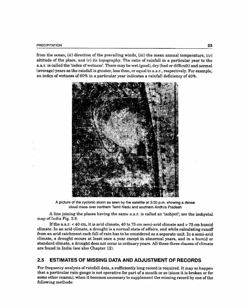
The application of radars in the study of storm mechanics, i.e. the areal extent, orientation andmovement of rain storms, is of great use. The radar signals reflected by the rain are helpful indetermining the magnitude of storm precipitation and its areal distribution. This method isusually used to supplement data obtained from a network of rain gauges. The IMD has a wellestablished radar network for the detection of thunder storms and six cyclone warning radars,on the east cost at Chennai, Kolkata, Paradeep, Vishakapatnam, Machalipatnam and Karaikal.See the picture given on facing page.
Location of rain-gauges—Rain-gauges must be so located as to avoid exposure to windeffect or interception by trees or buildings nearby.
The best location may be an open plane ground like an airport.The rainfall records are maintained by one or more of the following departments:
Indian Meteorological Department (IMD)Public Works Department (PWD)Agricultural DepartmentRevenue DepartmentForest Department, etc.
2.4 RAIN-GAUGE DENSITY
The following figures give a guideline as to the number of rain-gauges to be erected in agiven area or what is termed as ‘rain-gauge density’
Area Rain-gauge density
Plains 1 in 520 km2
Elevated regions 1 in 260-390 km2
Hilly and very heavy 1 in 130 Km2 preferably with 10% of the
rainfall areas rain-gauge stations equipped with the self
recording type
In India, on an average, there is 1 rain-gauge station for every 500 km2, while in moredeveloped countries, it is 1 stn. for 100 km2.
The length of record (i.e., the number of years) neeeded to obtain a stable frequencydistribution of rainfall may be recommended as follows:
Catchment layout: Islands Shore Plain Mountainousareas regions
No. of years: 30 40 40 50
The mean of yearly rainfall observed for a period of 35 consecutive years is called theaverage annual rainfall (a.a.r.) as used in India. The a.a.r. of a place depends upon: (i) distance

C-9\N-HYDRO\HYD2-1.PM5 24
24 HYDROLOGY
(i) Station-year method—In this method, the records of two or more stations are com-bined into one long record provided station records are independent and the areas in which thestations are located are climatologically the same. The missing record at a station in a particu-lar year may be found by the ratio of averages or by graphical comparison. For example, in acertain year the total rainfall of station A is 75 cm and for the neighbouring station B, there isno record. But if the a.a.r. at A and B are 70 cm and 80 cm, respectively, the missing year’srainfall at B (say, PB) can be found by simple proportion as:
7570
= PB
80∴ PB = 85.7 cm
This result may again be checked with reference to another neighbouring station C.(ii) By simple proportion (normal ratio method)–This method is illustrated by the fol-
lowing example.Example 2.1 Rain-gauge station D was inoperative for part of a month during which a stormoccured. The storm rainfall recorded in the three surrounding stations A, B and C were 8.5, 6.7and 9.0 cm, respectively. If the a.a.r for the stations are 75, 84, 70 and 90 cm, respectively,estimate the storm rainfall at station D.Solution By equating the ratios of storm rainfall to the a.a.r. at each station, the storm rain-fall at station D (PD) is estimated as
8 575.
= 6 784
9 070 90
. .= = PD
� The average value of PD = 13
8 575
906 784
909 070
90. . .× + × + ×L
NMOQP = 9.65 cm
(iii) Double-mass analysis—The trend of the rainfall records at a station may slightlychange after some years due to a change in the environment (or exposure) of a station eitherdue to coming of a new building, fence, planting of trees or cutting of forest nearby, whichaffect the catch of the gauge due to change in the wind pattern or exposure. The consistency ofrecords at the station in question (say, X) is tested by a double mass curve by plottting thecumulative annual (or seasonal) rainfall at station X against the concurrent cumulative valuesof mean annual (or seasonal) rainfall for a group of surrounding stations, for the number ofyears of record (Fig. 2.9). From the plot, the year in which a change in regime (or environment)has occurred is indicated by the change in slope of the straight line plot. The rainfall recordsof the station x are adjusted by multiplying the recorded values of rainfall by the ratio of slopesof the straight lines before and after change in environment.Example 2.2 The annual rainfall at station X and the average annual rainfall at 18 surround-ing stations are given below. Check the consistency of the record at station X and determine theyear in which a change in regime has occurred. State how you are going to adjust the recordsfor the change in regime. Determine the a.a.r. for the period 1952-1970 for the changed regime.
Annual rainfall (cm)
Year Stn. X 18-stn. average
1952 30.5 22.8
1953 38.9 35.0
1954 43.7 30.2
1955 32.2 27.4
(contd.)...

C-9\N-HYDRO\HYD2-1.PM5 25
PRECIPITATION 25
1956 27.4 25.2
1957 32.0 28.2
1958 49.3 36.1
1959 28.4 18.4
1960 24.6 25.1
1961 21.8 23.6
1962 28.2 33.3
1963 17.3 23.4
1964 22.3 36.0
1965 28.4 31.2
1966 24.1 23.1
1967 26.9 23.4
1968 20.6 23.1
1969 29.5 33.2
1970 28.4 26.4
Solution
Cumulative Annual rainfall (cm)
Year Stn. X 18-stn. average
1952 30.5 22.8
1953 69.4 57.8
1954 113.1 88.0
1955 145.3 115.4
1956 172.7 140.6
1957 204.7 168.8
1958 254.0 204.9
1959 282.4 233.3
1960 307.0 258.4
1961 328.8 282.0
1962 357.0 315.3
1963 374.3 338.7
1964 396.6 374.7
1965 425.0 405.9
1966 449.1 429.0
1967 476.0 452.4
1968 496.6 475.5
1969 526.1 508.7
1970 554.5 535.1
The above cumulative rainfalls are plotted as shown in Fig. 2.9. It can be seen from thefigure that there is a distinct change in slope in the year 1958, which indicates that a change inregime (exposure) has occurred in the year 1958. To make the records prior to 1958 comparable

C-9\N-HYDRO\HYD2-1.PM5 26
26 HYDROLOGY
with those after change in regime has occurred, the earlier records have to be adjusted bymultiplying by the ratio of slopes m2/m1 i.e., 0.9/1.25.
0 100 200 300 400 500 600
Cumulative annual rainfall-18 Stns. average, cm
Cum
ulat
ive
annu
alra
infa
llof
Stn
. X, c
m600
500
400
300
200
100
01952
1954
1956
1958
19601960
19621964
1966
1968
1970
2.5
2.5
1.8
1.8
22Change in regimeindicated in 1958
\´
Adjustment of records
prior to1958 : 0.91.25
Slop
e=
=1.
25=
m 1
2.5
2
Slope
=
=0.
9=
m 2
1.8
2
Fig. 2.9 Double mass analysis Example 2.2
Cumulative rainfall 1958-1970= 554.5 – 204.7 = 349.8 cm
Cumulative rainfall 1952-1957adjusted for changed environment
= 204.7 × 0 9125
..
= 147.6 cm
Cumulative rainfall 1952-1970(for the current environment) = 497.4 cma.a.r. adjusted for the current regime
= 497.4 cm19 years
= 26.2 cm.
2.6 MEAN AREAL DEPTH OF PRECIPITATION (Pave)
Point rainfall—It is the rainfall at a single station. For small areas less than 50 km2, pointrainfall may be taken as the average depth over the area. In large areas, there will be a net-work of rain-gauge stations. As the rainfall over a large area is not uniform, the average depthof rainfall over the area is determined by one of the following three methods:
(i) Arithmetic average method—It is obtained by simply averaging arithmetically theamounts of rainfall at the individual rain-gauge stations in the area, i.e.,

C-9\N-HYDRO\HYD2-1.PM5 27
PRECIPITATION 27
Pave = ΣPn
1 ...(2.1)
where Pave = average depth of rainfall over the areaΣP1 = sum of rainfall amounts at individual rain-gauge stations n = number of rain-gauge stations in the areaThis method is fast and simple and yields good estimates in flat country if the gauges
are uniformly distributed and the rainfall at different stations do not vary very widely fromthe mean. These limitations can be partially overcome if topographic influences and aerialrepresentativity are considered in the selection of gauge sites.
(ii) Thiessen polygon method—This method attempts to allow for non-uniform distribu-tion of gauges by providing a weighting factor for each gauge. The stations are plotted on abase map and are connected by straight lines. Perpendicular bisectors are drawn to the straightlines, joining adjacent stations to form polygons, known as Thiessen polygons (Fig. 2.10). Eachpolygon area is assumed to be influenced by the raingauge station inside it, i.e., if P1, P2, P3, ....are the rainfalls at the individual stations, and A1, A2, A3, .... are the areas of the polygonssurrounding these stations, (influence areas) respectively, the average depth of rainfall for theentire basin is given by
Pave = ΣΣA PA1 1
1...(2.2)
where ΣA1 = A = total area of the basin.The results obtained are usually more accurate than those obtained by simple arithme-
tic averaging. The gauges should be properly located over the catchment to get regular shapedpolygons. However, one of the serious limitations of the Thiessen method is its non-flexibilitysince a new Thiessen diagram has to be constructed every time if there is a change in theraingauge network.
(iii) The isohyetal method—In this method, the point rainfalls are plotted on a suitablebase map and the lines of equal rainfall (isohyets) are drawn giving consideration to orographiceffects and storm morphology, Fig. 2.11. The average rainfall between the succesive isohyetstaken as the average of the two isohyetal values are weighted with the area between theisohyets, added up and divided by the total area which gives the average depth of rainfall overthe entire basin, i.e.,
Pave = Σ
ΣA P
A1 2 1 2
1 2
− −
−...(2.3)
where A1–2 = area between the two successive isohyets P1 and P2
P1–2 = P P1 2
2+
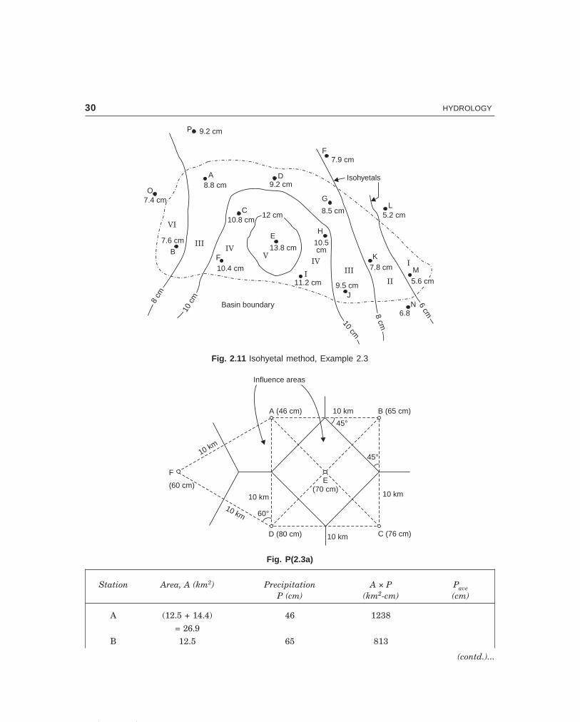
ΣA1–2 = A = total area of the basin.This method if analysed properly gives the best results.
Example 2.3 Point rainfalls due to a storm at several rain-gauge stations in a basin areshown in Fig. 2.10. Determine the mean areal depth of rainfall over the basin by the threemethods.

C-9\N-HYDRO\HYD2-1.PM5 28
28 HYDROLOGY
Basin boundary
Thiessenpolygons
LG
D
H
K
M
NJ
I
E
F
C
A
O
B
Stn.
Fig. 2.10 Thiessen polygon method, Example 2.3
Solution (i) Arithmetic average method
Pave = ΣPn
1 =1331cm15 stn.
= 8.87 cm
ΣP1 = sum of the 15 station rainfalls.(ii) Thiessen polygon method—The Thiessen polygons are constructed as shown in
Fig. 2.10 and the polygonal areas are planimetered and the mean areal depth of rainfall isworked out below:
Station Rainfall Area of influen- Product (2) × (3) Mean arealrecorded, P1 tial polygon, A1 A1P1 depth of
(cm) (km2) (km2-cm) rainfall
1 2 3 4 5
A 8.8 570 5016
B 7.6 920 6992
C 10.8 720 7776
D 9.2 620 5704
E 13.8 520 7176
F 10.4 550 5720
G 8.5 400 3400
H 10.5 650 6825
I 11.2 500 5600
J 9.5 350 3325
K 7.8 520 4056L 5.2 250 1300M 5.6 350 1960
Pave = ΣΣA PA1 1
1
= 667147180
= 9.30 cm
(contd.)...

C-9\N-HYDRO\HYD2-1.PM5 29
PRECIPITATION 29
N 6.8 100 680O 7.4 160 1184
Total 1331 cm 7180 km2 66714 km2-cm
n = 15 = ΣP1 = ΣA1 ΣA1P1
(iii) Isohyetal method—The isohyets are drawn as shown in Fig. 2.11 and the meanareal depth of rainfall is worked out below:
Zone Isohyets Mean isohyetal Area between Product Mean areal(cm) value, P1–2 isohyets, A1–2 (3) × (4) depth of
(cm) (km2) (km2-cm) rainfall(cm)
1 2 3 4 5 6
I <6 5.4 410 2214
II 6-8 7 900 6300
III 8-10 9 2850 25650
IV 10-12 11 1750 19250
V >12 12.8 720 9220
VI <8 7.5 550 4120
Total 7180 km2 66754 km2-cm= ΣA1–2 = ΣA1–2.P1–2
Example 2.3 (a) The area shown in Fig. P (2.3a) is composed of a square plus an equilateraltriangular plot of side 10 km. The annual precipitations at the rain-gauge stations located atthe four corners and centre of the square plot and apex of the traingular plot are indicated infigure. Find the mean precipitation over the area by Thiessen polygon method, and comparewith the arithmetic mean.Solution The Thiessen polygon is constructed by drawing perpendicular bisectors to the linesjoining the rain-gauge stations as shown in Fig. P (2.3a). The weighted mean precipitation iscomputed in the following table:
Area of square plot = 10 × 10 = 100 km2
Area of inner square plot = 10
2
10
2× = 50 km2
Difference = 50 km2
Area of each corner triangle in the square plot = 564 = 12.5 km2
13 area of the equilateral triangular plot = 1
3 ( 12 × 10 × 10 sin 60)
= 25
3 = 14.4 km2
Pave =
ΣΣ
A PA
1 2 1 2
1 2
− −
−
= 667547180
= 930 cm
C-9\N-HYDRO\HYD2-1.PM5 30
30 HYDROLOGY
VI
IIIIV
VIV
III
II
I
9.2 cm
8.8 cm 9.2 cmA D
C10.8 cm
12 cm12 cm
E
13.8 cm
H
10.5cm
11.2 cmI
9.5 cmJ
10cm
10cm
8cm
8cm
6cm
6cm6.8
N
M
5.6 cm5.6 cm
K7.8 cm
Basin boundary
10.4 cmF
10cm
10cm8
cm8
cm
7.6 cm
B
7.4 cmO
8.5 cm
GL
5.2 cm
Isohyetals
7.9 cm
P
F
Fig. 2.11 Isohyetal method, Example 2.3
10 km
60°10 km
D (80 cm)
F
(60 cm)
10 km
A (46 cm) 10 km B (65 cm)
45°
45°
Influence areas
10 km
E(70 cm)
C (76 cm)10 km
Fig. P(2.3a)
Station Area, A (km2) Precipitation A × P PaveP (cm) (km2-cm) (cm)
A (12.5 + 14.4) 46 1238
= 26.9
B 12.5 65 813
(contd.)...
C-9\N-HYDRO\HYD2-1.PM5 31
PRECIPITATION 31
C 12.5 76 950 = Σ
ΣA PA.
D (12.5 + 14.4) 80 2152 = 9517143 2.
= 26.9 = 66.3 cmE 50 70 3500
F 14.4 60 864
n = 6 ΣA = 143.2 ΣP = 397 ΣA.P. = 9517
= 100 + 25 3as a check
Arithmetic mean = ΣPn
= 3976
= 66.17 cm
which compares fairly with the weighted mean.
2.7 OPTIMUM RAIN-GAUGE NETWORK DESIGN
The aim of the optimum rain-gauge network design is to obtain all quantitative data averagesand extremes that define the statistical distribution of the hydrometeorological elements, withsufficient accuracy for practical purposes. When the mean areal depth of rainfall is calculatedby the simple arithmetic average, the optimum number of rain-gauge stations to be estab-lished in a given basin is given by the equation (IS, 1968)
N = CpvF
HGIKJ
2
...(2.4)
where N = optimum number of raingauge stations to be established in the basinCv = Coefficient of variation of the rainfall of the existing rain gauge stations (say, n) p = desired degree of percentage error in the estimate of the average depth of rainfall
over the basin.The number of additional rain-gauge stations (N–n) should be distributed in the differ-
ent zones (caused by isohyets) in proportion to their areas, i.e., depending upon the spatialdistribution of the existing rain-gauge stations and the variability of the rainfall over thebasin.
Saturated Newtork DesignIf the project is very important, the rainfall has to be estimated with great accuracy; then anetwork of rain-gauge stations should be so set up that any addition of rain-gauge stations willnot appreciably alter the average depth of rainfall estimated. Such a network is referred to asa saturated network.Example 2.4 For the basin shown in Fig. 2.12, the normal annual rainfall depths recordedand the isohyetals are given. Determine the optimum number of rain-gauge stations to be estab-lished in the basin if it is desired to limit the error in the mean value of rainfall to 10%. Indicatehow you are going to distribute the additional rain-gauge stations required, if any. What is thepercentage accuracy of the existing network in the estimation of the average depth of rainfallover the basin ?

C-9\N-HYDRO\HYD2-1.PM5 32
32 HYDROLOGY
Solution
Station Normal annual Difference (Difference)2 Statistical parametersrainfall, x (cm) (x – x ) (x – x )2 x , σ, Cv
A 88 – 4.8 23.0 x = Σxn
= 4645
B 104 11.2 125.4 = 92.8 cm
C 138 45.2 2040.0 σ = Σ( )x x
n−−
2
1
D 78 – 14.8 219.0 = 3767 45 1
.− = 30.7
E 56 – 36.8 1360.0
n = 5 Σx = 464 Σ(x – x )2 = 3767.4 Cv = σx
= 30 792 8
.
. × 100
= 33.1%
VI
IIIIV
VIV
III
II
I
88 cmA
120 cm120 cm
C
138 cm
100cm
100cm
80cm
80cm
60cm
60cm
E
56 cm56 cm
D78 cm104 cm
B
100
cm10
0cm
80cm
80cm
Isohyetals
Basin boundary
Fig. 2.12 Isohyetal map, Example 2.4
Note: x = Arithmetic mean, σ = standard deviation.
The optimum number of rain-gauge stations to limit the error in the mean value ofrainfall to p = 10%.
N = CpvF
HGIKJ = F
HGIKJ
2 233 110
. = 11
C-9\N-HYDRO\HYD2-1.PM5 33
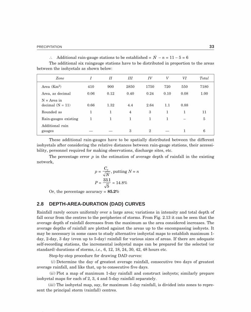
PRECIPITATION 33
∴ Additional rain-gauge stations to be established = �N – n = 11 – 5 = 6The additional six raingauge stations have to be distributed in proportion to the areas
between the isohyetals as shown below:
Zone I II III IV V VI Total
Area (Km2) 410 900 2850 1750 720 550 7180
Area, as decimal 0.06 0.12 0.40 0.24 0.10 0.08 1.00
N × Area indecimal (N = 11) 0.66 1.32 4.4 2.64 1.1 0.88
Rounded as 1 1 4 3 1 1 11
Rain-gauges existing 1 1 1 1 1 – 5
Additional raingauges — — 3 2 — 1 6
These additional rain-gauges have to be spatially distributed between the differentisohyetals after considering the relative distances between rain-gauge stations, their accessi-bility, personnel required for making observations, discharge sites, etc.
The percentage error p in the estimation of average depth of rainfall in the existingnetwork,
p = C
Nv , putting N = n
P = 33 1
5
. = 14.8%
Or, the percentage accuracy = 85.2%
2.8 DEPTH-AREA-DURATION (DAD) CURVES
Rainfall rarely occurs uniformly over a large area; variations in intensity and total depth offall occur from the centres to the peripheries of storms. From Fig. 2.13 it can be seen that theaverage depth of rainfall decreases from the maximum as the area considered increases. Theaverage depths of rainfall are plotted against the areas up to the encompassing isohyets. Itmay be necessary in some cases to study alternative isohyetal maps to establish maximum 1-day, 2-day, 3 day (even up to 5-day) rainfall for various sizes of areas. If there are adequateself-recording stations, the incremental isohyetal maps can be prepared for the selected (orstandard) durations of storms, i.e., 6, 12, 18, 24, 30, 42, 48 hours etc.
Step-by-step procedure for drawing DAD curves:(i) Determine the day of greatest average rainfall, consecutive two days of greatest
average rainfall, and like that, up to consecutive five days.(ii) Plot a map of maximum 1-day rainfall and construct isohyets; similarly prepare
isohyetal maps for each of 2, 3, 4 and 5-day rainfall separately.(iii) The isohyetal map, say, for maximum 1-day rainfall, is divided into zones to repre-
sent the principal storm (rainfall) centres.

C-9\N-HYDRO\HYD2-1.PM5 34
34 HYDROLOGY
(iv) Starting with the storm centre in each zone, the area enclosed by each isohyet isplanimetered.
(v) The area between the two isohyets multiplied by the average of the two isohyetalvalues gives the incremental volume of rainfall.
(vi) The incremental volume added with the previous accumulated volume gives thetotal volume of rainfall.
(vii) The total volume of rainfall divided by the total area upto the encompassing isohyetgives the average depth of rainfall over that area.
(viii) The computations are made for each zone and the zonal values are then combinedfor areas enclosed by the common (or extending) isohyets.
(ix) The highest average depths for various areas are plotted and a smooth curve isdrawn. This is DAD curve for maximum 1-day rainfall.
(x) Similarly, DAD curves for other standard durations (of maximum 2, 3, 4 day etc. or6, 12, 18, 24 hours etc.) of rainfall are prepared.Example 2.5 An isohyetal pattern of critical consecutive 4-day storm is shown in Fig. 2.13.Prepare the DAD curve.
Rain-gauge stations
10 cm10 cm
15 cm15 cm
20 cm20 cm
25 cm25 cm
30cm
30cm
35cm
35cm
+B
Stormcentres
+A
505045454040
3535cmcm
30cm
30cm
25cm
25cm
20cm
20cm
15cm
15cm10
cm10
cm
Fig. 2.13 Isohyetal pattern of a 4-day storm, Example 2.5

C-9\N-HYDRO\HYD2-1.PM5 35
PRECIPITATION 35
Solution Computations to draw the DAD curves for a 4-day storm are made in Table 2.1.Table 2.1.Computation of DAD curve (4-day critical storm)
Storm Encom Area Isohyetal Average Area Incremen- Total Averagecentre passing enclosed range isohyetal between tal volume volume depth
isohyet (km2) (cm) value isohyets (cm.km2) (cm.km2) (8) ÷ (3)(cm) (1000) (cm) (km2) (1000) (1000) (cm)
(1000)
1 2 3 4 5 6 7 8 9
A 50 0.5 > 50 say, 55 0.5 27.5 27.5 5540 4 40–50 45 3.5 157.5 185.0 46.2535 7 35–40 37.5 3 112.5 297.5 42.530 29 30–35 32.5 22 715.0 1012.5 34.91
B 35 2 > 35 say, 37.5 2 75.0 75.0 37.530 9.5 30–35 32.5 7.5 244.0 319.0 33.6
A 25 82 25–30 27.5 43.5 1196.2 2527.8 30.8122 20–25 22.5 40 900 3427.8 28.1
15 156 15–20 17.5 34 595 4022.8 25.8236 10–15 12.5 80 1000 5022.8 21.3
Plot ‘col. (9) vs. col. (3)’ to get the DAD curve for the maximum 4-day critical storm, asshown in Fig. 2.14.
00
40 80 120 160 200 240 280
Area in (1000 km2)
Ave
rage
dept
hcm
10
20
30
40
50
60
4-day storm
Fig. 2.14 DAD-curve for 4-day storm, Example 2.5
Isohyetal patterns are drawn for the maximum 1-day, 2-day, 3-day and 4-day (consecu-tive) critical rainstorms that occurred during 13 to 16th July 1944 in the Narmada and Tapticatchments and the DAD curves are prepared as shown in Fig. 2.15. The characteristics ofheavy rainstorms that have occurred during the period 1930–68 in the Narmada and Taptibasins are given below:
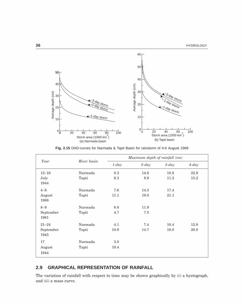
C-9\N-HYDRO\HYD2-1.PM5 36
36 HYDROLOGY
0 200 40 60 80 100Storm area (1000 km
2)
(a) Narmada basin
Ave
rage
dept
h(c
m)
50
40
30
50
20
10
0
3-day storm2-day storm
1-day storm
Storm area (1000 km2)
(b) Tapti basin
Ave
rage
dept
h(c
m)
0 20 40 60 100
60
50
40
30
20
10
0
3-day storm2-day storm1-day storm
Fig. 2.15 DAD-curves for Narmada & Tapti Basin for rainstorm of 4-6 August 1968
Year River basinMaximum depth of rainfall (cm)
1-day 2-day 3-day 4-day
13–16 Narmada 8.3 14.6 18.8 22.9July Tapti 6.3 9.9 11.2 15.21944
4–6 Narmada 7.6 14.5 17.4August Tapti 11.1 19.0 21.11968
8–9 Narmada 8.8 11.9September Tapti 4.7 7.51961
21–24 Narmada 4.1 7.4 10.4 12.9September Tapti 10.9 14.7 18.0 20.01945
17 Narmada 3.8
August Tapti 10.4
1944
2.9 GRAPHICAL REPRESENTATION OF RAINFALL
The variation of rainfall with respect to time may be shown graphically by (i) a hyetograph,and (ii) a mass curve.

C-9\N-HYDRO\HYD2-1.PM5 37
PRECIPITATION 37
A hyetograph is a bar graph showing the intensity of rainfall with respect to time(Fig. 2.16) and is useful in determining the maximum intensities of rainfall during a particu-lar storm as is required in land drainage and design of culverts.
16
14
12
10
8
6
4
2
0
Inte
nsity
ofra
infa
lli (
cm/h
r)
00 30 60 90 120 150 180 210
Time t (min)
3.54.0
12.0 cm/hr
210-min. storm
8.5
4.5
3.0
Fig. 2.16 Hyetograph
A mass curve of rainfall (or precipitation) is a plot of cumulative depth of rainfall againsttime (Fig. 2.17). From the mass curve, the total depth of rainfall and intensity of rainfall at anyinstant of time can be found. The amount of rainfall for any increment of time is the differencebetween the ordinates at the beginning and end of the time increments, and the intensity ofrainfall at any time is the slope of the mass curve (i.e., i = ∆P/∆t) at that time. A mass curve ofrainfall is always a rising curve and may have some horizontal sections which indicates peri-ods of no rainfall. The mass curve for the design storm is generally obtained by maximising themass curves of the severe storms in the basin.
Cum
ulat
ive
rain
fall
P,cm
7
6
5
4
3
2
1
012 AM 4 8 12 PM 4 8 12 AM 4 8 12 PM
Time t, hr
Intensity, i =Ñ p
t
ÑÑtt
ÑpMass curve ofprecipitation
Ñ
Fig. 2.17 Mass curve of rainfall

C-9\N-HYDRO\HYD2-1.PM5 38
38 HYDROLOGY
2.10 ANALYSIS OF RAINFALL DATA
Rainfall during a year or season (or a number of years) consists of several storms. The charac-teristics of a rainstorm are (i) intensity (cm/hr), (ii) duration (min, hr, or days), (iii) frequency(once in 5 years or once in 10, 20, 40, 60 or 100 years), and (iv) areal extent (i.e., area overwhich it is distributed).
Correlation of rainfall records—Suppose a number of years of rainfall records observedon recording and non-recording rain-gauges for a river basin are available; then it is possibleto correlate (i) the intensity and duration of storms, and (ii) the intensity, duration and fre-quency of storms.
If there are storms of different intensities and of various durations, then a relation maybe obtained by plotting the intensities (i, cm/hr) against durations (t, min, or hr) of the respec-tive storms either on the natural graph paper, or on a double log (log-log) paper, Fig. 2.18(a)and relations of the form given below may be obtained
(a) i = a
t b+ A.N. Talbot’s formula ...(2.5)
(for t = 5-120 min)
(b) i = k
tn ...(2.6)
(c) i = ktx ...(2.7)where t = duration of rainfall or its part, a, b, k, n and x are constants for a given region. Sincex is usually negative Eqs. (2.6) and (2.7) are same and are applicable for durations t > 2 hr. Bytaking logarithms on both sides of Eq. (2.7),
log i = log k + x log twhich is in the form of a straight line, i.e., if i and t are plotted on a log-log paper, the slope, ofthe straight line plot gives the constant x and the constant k can be determined as i = k whent = 1. Hence, the fitting equation for the rainfall data of the form of Eq. (2.7) can be determinedand similarly of the form of Eqs. (2.5) and (2.6).
On the other hand, if there are rainfall records for 30 to 40 years, the various stormsduring the period of record may be arranged in the descending order of their magnitude (ofmaximum depth or intensity). When arranged like this in the descending order, if there are atotal number of n items and the order number or rank of any particular storm (maximumdepth or intensity) is m, then the recurrence interval T (also known as the return period) of thestorm magnitude is given by one of the following equations:
(a) California method (1923), T = nm
....(2.8)
(b) Hazen’s method (1930), T = n
m − 12
...(2.9)
(c) Kimball’s method, (Weibull, 1939) T = n
m+ 1
...(2.10)
and the frequency F (expressed as per cent of time) of that storm magnitude (having recur-rence interval T) is given by
F = 1T
× 100% ...(2.11)

C-9\N-HYDRO\HYD2-2.PM5 39
PRECIPITATION 39
Natural paper
i = or i = ktxa
t + b
Time t (min or hr)
Inte
nsity
i(cm
/hr)
dydx
i = ktx
–x =dydx
Log-log paperi = k
Inte
nsity
i(cm
/hr)
Time t (min or hr)1
(a) Correlation of intensity and duration of storms
Inte
nsity
i(cm
/hr)
T = 15-yearT = 10-yearT = 5-yearT = 1-year
Naturalpaper
i =kT
t
x
e
Time t (min or hr) Time t (min or hr)
Inte
nsity
i(cm
/hr)
A : High intensity for short durationB : Low intensity for long duration
i = k
i1
Ñlog i Ñ
log t
A
x = log i
i2
1
i2
ÑÑlog ilog tlog ilog t
ÑÑ– e =– e =
One logcycle of T
One logcycle of T
Log-log paperLog-log paperi = kT
t
x
e
Dec
reas
ing
frequ
ency
T = 50-year
T = 20-yearT = 15-year
T = 15-yearT = 5-yearT = 5-yearT = 1-yearT = 1-year
B
(b) Correlation of intensity, duration and frequency of storms
1
Fig. 2.18 Correlation of storm characteristics
Values of precipitation plotted against the percentages of time give the ‘frquency curve’.All the three methods given above give very close results especially in the central part of thecurve and particularly if the number of items is large.
Recurrence interval is the average number of years during which a storm of given mag-nitude (maximum depth or intensity) may be expected to occur once, i.e., may be equalled orexceeded. Frequency F is the percentage of years during which a storm of given magnitudemay be equalled or exceeded. For example if a storm of a given magnitude is expected to occuronce in 20 years, then its recurrence interval T = 20 yr, and its frequency (probability ofexceedence) F = (1/20) 100 = 5%, i.e., frequency is the reciprocal (percent) of the recurrenceinterval.
The probability that a T-year strom and frequency FT
= ×FHG
IKJ
1100% may not occur in
any series of N years isP(N, 0) = (1 – F)N ...(2.12)

C-9\N-HYDRO\HYD2-2.PM5 40
40 HYDROLOGY
and that it may occur isPEx = 1 – (1 – F)N ...(2.12a)
where PEx = probability of occurrence of a T-year storm in N-years.The probability of a 20-year storm (i.e., T = 20, F = 5%) will not occur in the next 10 years
is (1 – 0.05)10 = 0.6 or 60% and the probability that the storm will occur (i.e., will be equalled orexceeded) in the next 10 years is 1 – 0.6 = 0.4 or 40% (percent chance).
See art. 8.5 (Encounter Probability), and Ex. 8.6 (a) and (b) (put storm depth instead offlood).
If the intensity-duration curves are plotted for various storms, for different recurrenceintervals, then a relation may be obtained of the form
i = kT
t
x
e ... Sherman ...(2.13)
where k, x and e are constants.‘i vs. t’ plotted on a natural graph paper for storms of different recurrence intervals
yields curves of the form shown in Fig. 2.18 (b), while on a log-log paper yields straight lineplots. By taking logarithms on both sides of Eq. (2.13),
log i = (log k + x log T) – e log twhich plots a straight line; k = i, when T and t are equal to 1. Writing for two values of T (forthe same t) :
log i1 = (log k + x log T1) – e log tlog i2 = (log k + x log T2) – e log t
Subtracting, log i1 – log i2 = x (log T1 – log T2)
or, x = ∆∆
loglog
iT
∴ x = charge in log i per log-cycle of T (for the same value of t)Again writing for two values of t (for the same T):
log i1 = (log k + x log T) – e log t1
log i2 = (log k + x log T) – e log t2
Subtracting log i1 – log i2 = – e(log t1 – log t2)
or –e = loglog
it
or e = – slope = ∆∆
loglog
it
∴ e = change in log i per log cycle of t (for the same value of T).The lines obtained for different frequencies (i.e., T values) may be taken as roughly
parallel for a particular basin though there may be variation in the slope ‘e’. Suppose, if a 1-year recurrence interval line is required, draw a line parallel to 10–year line, such that thedistance between them is the same as that between 5-year and 50-year line; similarly a 100-year line can be drawn parallel to the 10-year line keeping the same distance (i.e., distance perlog cycle of T). The value of i where the 1-year line intersects the unit time ordinate (i.e., t = 1min, say) gives the value of k. Thus all the constants of Eq. (2.13) can be determined from thelog-log plot of ‘i vs. t’ for different values of T, which requires a long record of rainfall data.Such a long record, will not usually be available for the specific design area and hence it
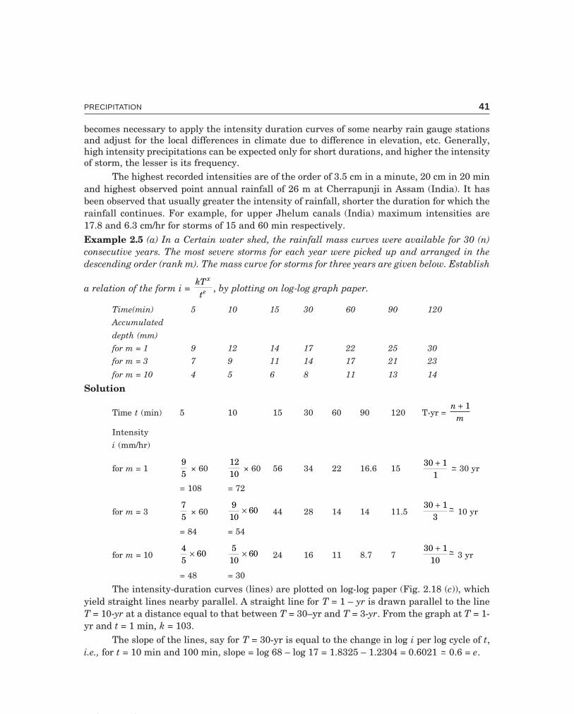
C-9\N-HYDRO\HYD2-2.PM5 41
PRECIPITATION 41
becomes necessary to apply the intensity duration curves of some nearby rain gauge stationsand adjust for the local differences in climate due to difference in elevation, etc. Generally,high intensity precipitations can be expected only for short durations, and higher the intensityof storm, the lesser is its frequency.
The highest recorded intensities are of the order of 3.5 cm in a minute, 20 cm in 20 minand highest observed point annual rainfall of 26 m at Cherrapunji in Assam (India). It hasbeen observed that usually greater the intensity of rainfall, shorter the duration for which therainfall continues. For example, for upper Jhelum canals (India) maximum intensities are17.8 and 6.3 cm/hr for storms of 15 and 60 min respectively.Example 2.5 (a) In a Certain water shed, the rainfall mass curves were available for 30 (n)consecutive years. The most severe storms for each year were picked up and arranged in thedescending order (rank m). The mass curve for storms for three years are given below. Establish
a relation of the form i = kTt
x
e , by plotting on log-log graph paper.
Time(min) 5 10 15 30 60 90 120
Accumulated
depth (mm)
for m = 1 9 12 14 17 22 25 30
for m = 3 7 9 11 14 17 21 23
for m = 10 4 5 6 8 11 13 14
Solution
Time t (min) 5 10 15 30 60 90 120 T-yr = n
m+ 1
Intensity
i (mm/hr)
for m = 195
× 601210
× 60 56 34 22 16.6 1530 1
1+
~− 30 yr
= 108 = 72
for m = 375
× 60910
60× 44 28 14 14 11.530 1
3+ −~ 10 yr
= 84 = 54
for m = 1045
60× 510
60× 24 16 11 8.7 730 1
10+ −~ 3 yr
= 48 = 30
The intensity-duration curves (lines) are plotted on log-log paper (Fig. 2.18 (c)), whichyield straight lines nearby parallel. A straight line for T = 1 – yr is drawn parallel to the lineT = 10-yr at a distance equal to that between T = 30–yr and T = 3-yr. From the graph at T = 1-yr and t = 1 min, k = 103.
The slope of the lines, say for T = 30-yr is equal to the change in log i per log cycle of t,i.e., for t = 10 min and 100 min, slope = log 68 – log 17 = 1.8325 – 1.2304 = 0.6021 ~− 0.6 = e.
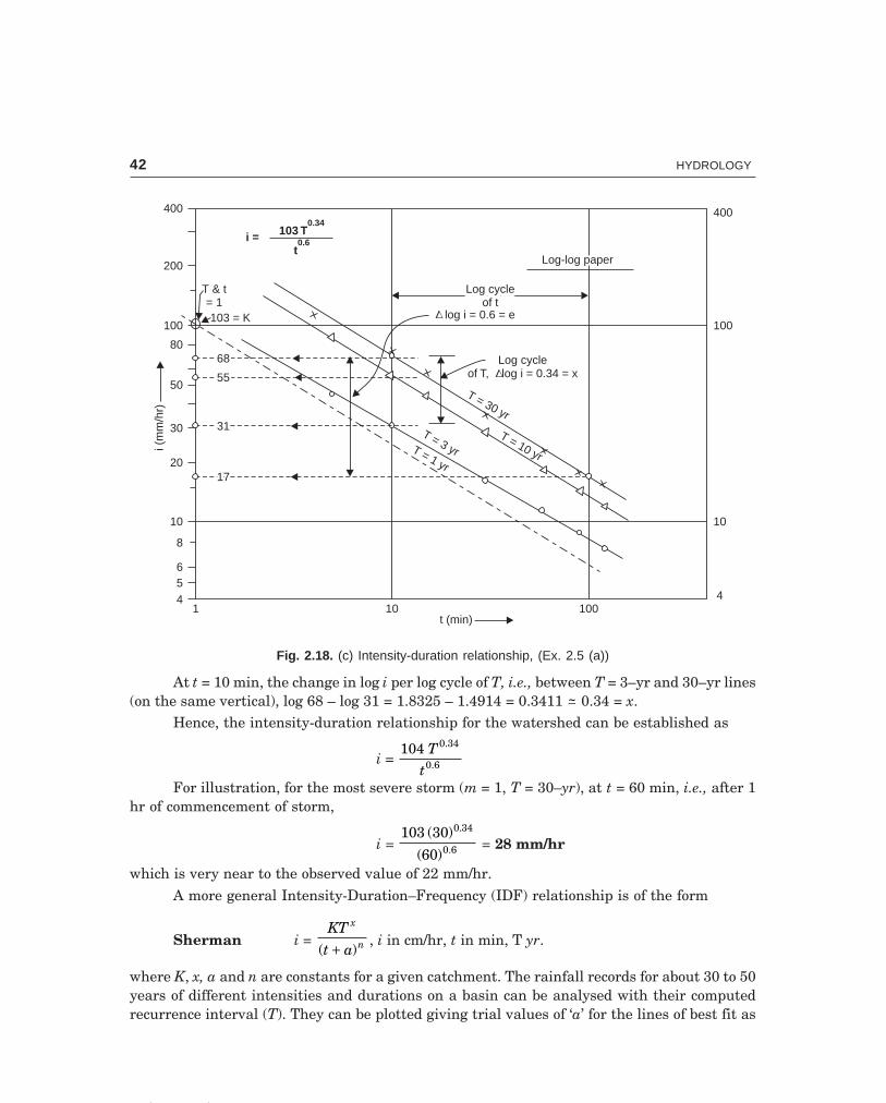
C-9\N-HYDRO\HYD2-2.PM5 42
42 HYDROLOGY
400
200
100
80
50
30
20
10
8
654
1 10 1004
10
100
400
i = 103 T
t
0.34
0.6
Log-log paperLog-log paper
Log cycleof t
Log cycleof tÑ
log i = 0.6 = e
Log cycleof T, log i = 0.34 = x
T = 30 yr
6868
5555
3131
1717
T = 1 yr
Ñ
T = 3 yr
T & t= 1103 = K
T = 10 yr
t (min)
i(m
m/h
r)
Fig. 2.18. (c) Intensity-duration relationship, (Ex. 2.5 (a))
At t = 10 min, the change in log i per log cycle of T, i.e., between T = 3–yr and 30–yr lines(on the same vertical), log 68 – log 31 = 1.8325 – 1.4914 = 0.3411 ~− 0.34 = x.
Hence, the intensity-duration relationship for the watershed can be established as
i = 104 0.34
0.6T
tFor illustration, for the most severe storm (m = 1, T = 30–yr), at t = 60 min, i.e., after 1
hr of commencement of storm,
i = 103 30
60
0.34
0.6
( )
( ) = 28 mm/hr
which is very near to the observed value of 22 mm/hr.A more general Intensity-Duration–Frequency (IDF) relationship is of the form
Sherman i = KT
t a
x
n( )+ , i in cm/hr, t in min, T yr.
where K, x, a and n are constants for a given catchment. The rainfall records for about 30 to 50years of different intensities and durations on a basin can be analysed with their computedrecurrence interval (T). They can be plotted giving trial values of ‘a’ for the lines of best fit as

C-9\N-HYDRO\HYD2-2.PM5 43
PRECIPITATION 43
shown in Fig. 2.18 (b). The values of a and n may be different for different lines of recurrenceinterval.
The constants can also be obtained by multiple regression model based on the principleof least squares and solutions can be obtained by computer-based numerical analysis; confi-dence intervals for the predictions can be developed.
Extreme point rainfall values of different durations and recurrence interval (returnperiod) have been evaluated by IMD and the ‘isopluvial maps’ (lines connecting equal depthsof rainfall) for the country prepared.Example 2.5 (b) A small water shed consists of 2 km2 of forest area (c = 0.1), 1.2 km2 of culti-vated area (c = 0.2) and 1 km2 under grass cover (c = 0.35). A water course falls by 20 m in alength of 2 km. The IDF relation for the area may be taken as
i = 80
12
0.2
0.5
Tt( )+
, i in cm/hr, t in min and T yr
Estimate the peak rate of runoff for a 25 yr frequency.Solution Time of concentration (in hr)
tc = 0.06628 L0.77 S–0.385, Kirpich’s formula, L in km
= 0.06628 × 20.77 20
2 1000
0.385
×FHG
IKJ
−
= 0.667 hr × 60 = 40 min.
i = ic when t = tc in the given IDF relation
∴ ic = 80 2540 12
0.2
0.5
×+( )
= 21.1 cm/hr
Qpeak = 2.78 C ic A, rational formula, CA = ΣCiAi
= 2.78 × 21.1 × (0.1 × 2 + 0.2 × 1.2 + 0.35 × 1) = 46.4 cumec
2.11 MEAN AND MEDIAN
The sum of all the items in a set divided by the number of items gives the mean value,i.e.,
x = Σxn
...(2.10)
where x = the mean valueΣx = sum of all the items n = total number of items.The magnitude of the item in a set such that half of the total number of items are larger
and half are smaller is called the median. The apparent median for the curve in Fig. 2.21 is theordinate corresponding to 50% of the years. The mean may be unduly influenced by a few largeor small values, which are not truly representative of the samples (items), whereas the medianis influenced mainly by the magnitude of the main part of intermediate values.
To find the median, the items are arranged in the ascending order; if the number ofitems is odd, the middle item gives the median; if the number of items is even, the average ofthe central two items gives the median.

C-9\N-HYDRO\HYD2-2.PM5 44
44 HYDROLOGY
Example 2.6 The annual rainfall at a place for a period of 10 years from 1961 to 1970 arerespectively 30.3, 41.0, 33.5, 34.0, 33.3, 36.2, 33.6, 30.2, 35.5, 36.3. Determine the mean andmedian values of annual rainfall for the place.
Solution (i) Mean x = Σxn
= (30.3 + 41.0 + 33.5 + 34.0 + 33.3 + 36.2
+ 33.6 + 30.2 + 35.5 + 36.3)/10
= 343 9
10.
= 34.39 cm
(ii) Median: Arrange the samples in the ascending order 30.2, 30.3 33.3, 33.5, 33.6, 34.0,35.5, 36.2, 36.3, 41.0
No. of items = 10, i.e., even
∴ Median = 33 6 34 0
2. .+
= 33.8 cm
Note the difference between the mean and the median values. If 11 years of record, say1960 to 1970, had been given, the median would have been the sixth item (central value) whenarranged in the ascending order.
Example 2.7 The following are the rain gauge observations during a storm. Construct: (a)mass curve of precipitation, (b) hyetograph, (c) maximum intensity-duration curve and developa formula, and (d) maximum depth-duration curve.
Time since commencement Accumulatedof storm rainfall
(min) (cm)
5 0.1
10 0.2
15 0.8
20 1.5
25 1.8
30 2.0
35 2.5
40 2.7
45 2.9
50 3.1
Solution (a) Mass curve of precipitation. The plot of ‘accumulated rainfall (cm) vs. time(min)’ gives the ‘mass curve of rainfall’ Fig. 2.19 (a).
(b) Hyetograph. The intensity of rainfall at successive 5 min interval is calculated and abar-graph of ‘i (cm/hr) vs. t (min)’ is constructed; this depicts the variation of the intensity ofrainfall with respect to time and is called the ‘hyetograph; 2.19 (b).

C-9\N-HYDRO\HYD2-2.PM5 45
PRECIPITATION 45
Time, t Accumulated ∆ P in time Intensity,(min) rainfall ∆t = 5 min
i = ∆∆Pt
× 60
(cm) (cm) (cm/hr)
5 0.1 0.1 1.2
10 0.2 0.1 1.2
15 0.8 0.6 7.2
20 1.5 0.7 8.4
25 1.8 0.3 3.6
30 2.0 0.2 2.4
35 2.5 0.5 6.0
40 2.7 0.2 2.4
45 2.9 0.2 2.4
50 3.1 0.2 2.4
3.5
3.0
2.5
2.0
1.5
1.0
0.5
0
Tota
lrai
nfal
ldep
th(c
m)
mass curve traced byself-recording rain gauge
50-min storm
0 5 10 15 20 25 30 35 40 45 50 55 60
Time t (min)
Ñ pt
Ñi =
Ñt
Ñp
(a) Mass curve of precipitation
1.2 cm/hr
8.4 cm/hr
2.4 cm/hr
7.2
3.6
2.4
6.0
50-min storm
Area under the curvegives total precipitation (cm)
Inte
nsity
i(cm
/hr)
10
8
6
4
2
00 5 10 15 20 25 30 35 40 450 50
Time t (min)
(b) Hyetograph
Fig. 2.19 Graphs from recording rain-gauge data, Example 2.7
(c) Maximum depth–duration curve. By inspection of time (t) and accumulated rainfall(cm) the maximum rainfall depths during 5, 10, 15, 20, 25, 30, 35, 40, 45 and 50 min durations

C-9\N-HYDRO\HYD2-2.PM5 46
46 HYDROLOGY
are 0.7, 1.3, 1.6, 1.8, 2.3, 2.5, 2.7, 2.9, 3.0 and 3.1 cm respectively. The plot of the maximumrainfall depths against different durations on a log-log paper gives the maximum depth-dura-tion curve, which is a straight line, Fig. 2.20 (a).
i = 17
t0.375
b. Maximum intensity-duration curveb. Maximum intensity-duration curve
a. Maximum depth-duration curvea. Maximum depth-duration curve
k = 17
x = – 0.3750.75cm
Log-log paper
100
80
60
40
30
20
15
10
8
65
4
3
2
1.5
1
Inte
nsity
i(cm
/hr)
1 1.5 2 3 4 5 6 8 10 15 20 30 40 60 80 100
10
8
6
4
3
2
1.5
1
0.8
0.6
0.4
0.3
0.2
0.15
2.0 cm2.0 cm
0.1
Max
imum
dept
h(c
m)
Time t (min)
Slope
Fig. 2.20 Maximum depth-duration & intensity-duration curves (Example 2.7)
(d) Maximum intensity-duration curve. Corresponding to the maximum depths obtained
in (c) above, the corresponding maximum intensities can be obtained ∆∆Pt
× 60, i.e., 8.4, 7.8, 6.4,
5.4, 5.52, 5.0, 4.63, 4.35, 4.0 and 3.72 cm/hr, respectively. The plot of the maximum intensitiesagainst the different duration on a log-log paper gives the maximum intensity-duration curvewhich is a straight line, Fig. 2.20 (b).
The equation for the maximum itensity duration curve is of the form i = ktx
Slope of the straight line plot,
– x = dydx
= 0.75 cm2.00 cm = 0.375
k = 17 cm/hr when t = 1 minHence, the formula becomes
i = 170.375t
which can now be verified ast = 10 min, i = 7.2 cm/hrt = 40 min, i = 4.25 cm/hr
which agree with the observed data

C-9\N-HYDRO\HYD2-2.PM5 47
PRECIPITATION 47
Example 2.8 The annual rainfall at a place for a period of 21 years is given below. Draw therainfall frequency curve and determine :
(a) the rainfall of 5-year and 20-year recurrence, interval(b) the rainfall which occurs 50% of the times(c) the rainfall of probability of 0.75(d) the probability of occurrence of rainfall of 75 cm and its recurrence interval.
Year Rainfall Year Rainfall(cm) (cm)
1950 50 1961 561951 60 1962 521952 40 1963 421953 27 1964 381954 30 1965 271955 38 1966 401956 70 1967 1001957 60 1968 901958 35 1969 441959 55 1970 33
1960 40
Solution Arrange the yearly rainfall in the descending order of magnitude as given below. Ifa particular rainfall occurs in more than one year, m = no. of times exceeded + no. of timesequalled.
Year Rainfall Rank (m) Frequency
P (cm) (no. of times ≥ P) F = m
n + 1 × 100%
1967 100 1 4.61968 90 2 9.11956 70 3 13.6
1951, 1957 60 5 22.71961 56 6 27.31959 55 7 31.81962 52 8 36.41950 50 9 40.91969 43 10 45.51963 42 11 50.0
1952 19601966
, UVW 40 14 63.7
1955, 1964 38 16 72.81958 35 17 77.31970 33 18 81.81954 30 19 86.4
1953, 1965 27 21 95.5
Total Σx = 1026 n = 21

C-9\N-HYDRO\HYD2-2.PM5 48
48 HYDROLOGY
Draw the graph of ‘P vs. F’ on a semi-log paper which gives the rainfall frequency curve,Fig. 2.21. From the frequency-curve, the required values can be obtained as
(a) T = 5–yr, F = 1T
× 100 = 1005
= 20% for which P = 64 cm.
T = 20 – yr, F = 1
20 × 100 = 5% for which P = 97.5 cm
0
10
20
30
40
50
60
70
80
90
100
100 50 25 20 10 5 2 1
Semi-log paper
97.5 cm
75 cm
64 cm
48.8 cm
42.2 cm
32 cm
Frequencycurve
MeanMedianMedian
1 1.5 2 3 4 5 6 7 8 10 15 20 30 40 50 60 80 100
Frequency F % ( P)£
Ann
ual r
ainf
all P
(cm
)
12.4 % 37 %37 % 75 %75 %
Recurrence interval T-yr
8 yr
Fig. 2.21 Rainfall frequency curve (Example 2.8)
(b) For F = 50%, P = 42.2 cm which is the median value, and the mean value
x = Σxn
= 102621
= 48.8 cm
which has a frequency of 37%.(c) For a probability of 0.75 F = 75% for which P = 32 cm
(d) For P = 75 cm, F = 12.4%, T = 1F
× 100 = 10012 4.
= 8 yr
and its probability of occurrence = 0.124
2.12 MOVING AVERAGES CURVE
If the rainfall at a place over a number of years is plotted as a bar graph it will not show anytrends or cyclic patterns in the rainfall due to wide variations in the consecutive years. In

C-9\N-HYDRO\HYD2-2.PM5 49
PRECIPITATION 49
order to depict a general trend in the rainfall pattern, the averages of three or five consecutiveyears are found out progressively by moving the group averaged, one year at a time. In Fig.2.22, the 21-years of rainfall records at a place given in Example 2.8 are shown. The first fiveyears of record are averaged as (50 + 60 + 40 + 27 + 30)/5 = 207/5 = 41.4 cm and this average isplotted at the mid-point of the group. The next point is obtained by omitting the first andaveraging the 2 to 6 years of record, again plotting the average i.e., (207 – 50 + 38)/5 = 39 cm atthe midpoint of this group, and so on as shown in Fig. 2.22. Thus, a 5-year moving mean curveis obtained in which the wide variations in the consecutive years are smoothed out. A 3-year or5-year moving mean curve is useful in identifying the long term trends or patterns in therainfall at a place.
5-year moving mean curve trend line
1950 51 52 53 54 55 56 57 58 59
1960 6261 63 64 65 66 67 68 69
1970
Years
100
80
60
40
20
0
Pre
cipi
tatio
nP
(cm
)
Fig. 2.22 Trends from moving mean curves (Example 2.8)
The same techniques may be applied to other hydrometeorogical parameters like tem-perature, hours of bright sunshine, wind speeds, cloud cover, etc.
2.13 DESIGN STORM AND PMP
For the safe design of structures even a 50-year or 100-year precipitation may be inadequatedue to the unusual meteorological combinations resulting in very high precipitation. The mostcritical features of several past storms are often combined, for a given frequency of occurrence,into a single design storm (hypothetical) for the purpose of design of important structures. Theprobable maximum precipitation (PMP) for a given region is the precipitation resulting fromthe most critical meteorogical combinations that are considered probable of occurrence. Thisconcept of PMP is very important in estimating the maximum probable flood in the safe designof flood control structures, spillways for dams, etc. PMP can be estimated by maximising thedifferent parameters like wind velocity, humidity etc. of an observed severe storm over thebasin. When sufficient data of storms for a given basin is not available, PMP can be estimatedfrom a severe storm on the adjacent basin and storm transposition.
2.14 SNOW PACK AND SNOW MELT
Snow melts due to heat from the atmosphere, from the warm rainfall and by radiation. On thebasis of measurement of snow depth and water equivalent (or density) of snow at grid stations

C-9\N-HYDRO\HYD2-2.PM5 50
50 HYDROLOGY
along the snow courses, the water storage in the snow (i.e., the available snow melt) can bedetermined from the formula.
dw = Gsds ...(2.11)
where dw = depth of water storage in the snow
ds = depth of snow cover
Gs = water equivalent (density) of snow
Water equivalent or snow density is the ratio of the volume of melt water from a sampleof snow to the initial volume of the snow sample. An average density of 0.1 for freshly fallensnow is often assumed; however the longer the snow remains on the ground, the denser itbecomes due to packing, alternate thawing and freezing, condensation and the presence ofabsorbed rainfall and melt water. Snow density will be about 0.1 at the beginning of winterand about 0.3 at the end of winter, i.e., at the beginning of thaw. The density of snow varieswith depth and so samples must be taken at various horizons in a snow pack for determiningthe water equivalent. This is usually done by a sampling tube. Snowfall may be measureddirectly by an ordinary rain gauge fitted with a heating system, or by a simple snow stake, ifthere is no drifting and density is determined simultaneously.
Snow surveys are made by dividing the basin into rectangular grids and determiningthe snow depths and densities at depths at the grid stations. From the water equivalents thusobtained at individual stations, the average water equivalent of the snow pack over the entirebasin can be derived by the same method used for determining the mean areal depth of rainfall.In India, snow surveys are generally conducted in the beginning of summer, i.e., in March orApril, when snow starts melting. Many of the perennial rivers in north India are fed by snow-melt from the Himalayan range in summer. In the Himalayan range, one-tenth of the depth ofsnow is added to the depth of rainfall, as a thumb rule, to obtain the total precipitation.
Also see Appendix-A.
�������
I Match the items in ‘A’ with items in ‘B’:
A B
(i) Cyclone (a) Optimum rain-gauge network
(ii) Frontal surface (b) Intensity of storm
(iii) Rain-gauge (c) Can not record snow
(iv) Double mass curve (d) 1 in 500 km2
(v) Tipping bucket gauge (e) Mean areal depth of precipitation
(vi) Recording rain-gauge (f) Western Ghats (of Peninsular India)
(vii) Orographic precipitation (g) Covergence of storm
(viii) Thiessen network (h) Surface of contact between warm andcold air masses
(ix) Raingauge density (i) Air port
(x) Coefficient of variation, Cv (j) Change of regime of rain-gauge station

C-9\N-HYDRO\HYD2-2.PM5 51
PRECIPITATION 51
II Fill up the blanks in the following:
(i) Rain-gauges are erected...... over the ground surface with their rim at .... cm above groundsurface
(ii) The three principal agencies, which maintain rain-gauges and make observations in Karnatakaare: (a) ....... (b) ........ and (c) ......
(iii) Rain-gauge readings are taken every day at .... hr IST
(iv) In coastal areas of Karnataka one rain-gauge should be erected for every ..... km2 and .......years (consecutive) of record are required for statistical analysis.
(v) An index of wetness of 40% in a certain area indicates a ..... year with a rainfall deflciency of....%.
III Say ‘True’ or ‘False’; if false, give the correct statement:
(i) Rain-gauges are erected perpendicular to the ground surface on which they are installed.
(ii) Cyclonic precipitation is due to convergence of storms towards a low pressure belt.
(iii) In hilly and heavy rainfall areas at least 10% of the rain-gauges should be of self-recordingtype.
(iv) As the area increases, the average depth of precipitation increases for a particular storm.
(v) Generally, high intensity precipitation can be expected only for short durations, and higherthe intensity, lesser is its frequency.
(vi) The coefficient of variation for annual precipitation data is equal to the standard deviation ofthe indices of wetness.
(vii) A mass curve of rainfall need not always be a rising curve.
(viii) The longer the snow remains on the ground, the less dense it becomes.
(ix) The intensity of storm is an inverse function of its duration. (false: i, iv, vii, viii)
IV Choose the correct statement/s in the following:1 Precipitation includes
(i) rainfall (ii) snow melt(iii) hail storm (iv) stream flow(v) mist and fog (vi) frost
(vii) all the above2 In a cold front
(i) cold air mass drives out a warm air mass(ii) warm air mass replaces the retreating cold air mass
(iii) cold air and warm air masses are drawn simultaneously towards a low pressure area(iv) the cold and warm air masses are stationary
3 Cyclonic precipitation is due to(i) orographic lifting (ii) ocean nearby
(iii) convergence of storms towards a low pressure belt(iv) divergence of storms (v) thermal convection(vi) conflict between cold and warm air masses
4 A self-recording rain-gauge(i) records by hourly depth of rain (ii) records the snow melt
(iii) records the cumulative depth of rainfall(iv) records the rainfall intensity (v) records the onset and cessation of rainfall(vi) records the cloud cover

C-9\N-HYDRO\HYD2-2.PM5 52
52 HYDROLOGY
5 A double mass analysis is made(i) to find the missing rainfall at a station in a particular area
(ii) to detect any change in exposure of a station
(iii) to adjust the record at a station to the changed environment
(iv) to compute the a.a.r. consistent with the changed environment
(v) for all the above purposes
6 Isohyetal method gives accurate mean areal depth of rainfall
(i) in a plain country
(ii) in a gently sloping basin
(iii) in an undulating country
(iv) in places of known storm movement
(v) in a basin consisting of plains and hills
(vi) when there are optimum number of rain-gauge stations
(vii) when the precipitation includes snowmelt
(1-exept iv; 2–i ; 3–iii ; 4–iii, v ; 5–ii, iii, iv ; 6–iii, iv, v)
�������
1 What factors you consider in selecting a site for a rain-gauge station?2 (a) Distinguish between recording and non-recording rain-gauges, giving examples of such gauges
used in India.(b) Which are the agencies that usually maintain rain-gauges and make observations in your
State? At what time or times in the day is the rainfall recorded?3 What are the different forms of precipitation ? Which of them are of significance to a civil engi-
neer ?4 (a) Explain: (i) a method for estimating the missing rainfall data at a station in a basin.
(ii) a method for testing the consistency of rainfall records at a station and necessaryadjustment.
(b) A 3-hour storm occurred at a place and the precipitations in the neighbouring rain-gaugestations P, Q and R were measured as 3.8, 4.1 and 4.5 cm, respectively. The precipitation inthe neighbouring station S could not be measured since the rain-gauge bottle was broken.The normal precipitation in the four stations P, Q, R and S as per IMD Bulletin were 45, 48,53 and 50 cm, respectively. Estimate the storm precipitation at station S. (4.246 cm)
5 (a) Define ‘rain-gauge density’ and explain how you would determine the optimum number ofrain-gauges to be erected in a given basin.
(b) In a certain river basin there are six rain-gauge stations, the normal annual rainfall depthsat the stations being 42.4, 53.6, 67.8, 78.5, 82.7 and 95.5 cm, respectively. Determine theoptimum number of rain-gauge stations to be established in the basin if it is desired to limitthe error in the mean value of rainfall over the catchment to 10% and indicate how youdistribute them, (7)
6 For the basin shown in Fig. P 2.23, the normal annual rainfall depths recorded and the isohyetalsare given. Determine the optimum number of rain-gauge stations to be established in the basinif it is desired to limit the error in the mean value of rainfall to 10%. Indicate how you are goingto distribute the additional rain-gauge stations required if any. What is the percentage accuracy

C-9\N-HYDRO\HYD2-2.PM5 53
PRECIPITATION 53
of the exixting network in the estimation of the average depth of rainfall over the basin. Thearea between the isohyetals are given below :Zone: I II III IV V VI Total
Area (Km2): 63 278 389 220 55 33 1038
(16—1, 1, 4, 2, 0, 1; 85.2%)
VI
III
I
II
III
IV
V
50 cm
75 cm
60 cmA
F
B
86 cm
100cm100cm
92 cm
68 cmG
75cm
50cm
25cm
D
45 cm
20 cm20 cm
E
C62 cm
Fig. P2.23 Isohyetal map
7 (a) Explain three methods of determining the mean areal depth of precipitation over a basincovered by several rain-gauge stations.
(b) Find the mean precipitation for the area shown in Fig. P 2.24 by Thiessen polygon method.The area is composed of a square plus an equilateral triangular plot of side 2 km. Rainfallreadings are in cm at the various stations indicated. (32.33 cm)
2 km
D
F 15 cm
2 km
A 2 km B
2 kmE
C
38 cm
20 cm
10 cm68 cm
43 cm
Rain gauge stations
Fig. P2.24 Rain-gauge network

C-9\N-HYDRO\HYD2-2.PM5 54
54 HYDROLOGY
8 Thiessen polygons and isohyetal map are given in Fig. P 2.25 and P 2.26, respectively, for differ-ent drainage basins. Areas and precipitation values are tabulated. Compute the average precipi-tation over the basins.
Station Thiessen polygon Precipitationarea (cm)(km2)
A 170 9.3
B 164 10.5
C 156 10.9
D 150 12.2
E 116 13.5
F 36 14.0
G 124 14.2
H 42 12.8
Area of basin = 958 km2
Zone Area (km2)
I 56
II 192
III 420
IV 244
V 44
VI 58
Area of basin = 1014 km2
A
9.3 cm
12.8 cm
H
G
14.2 cm
14.0 cm
FC
10.9 cm
10.5 cm
B
D
12.2 cm 13.5 cm
E
Basin boundary
Polygonal areas
Fig. P2.25 Thiessen polygons
C-9\N-HYDRO\HYD2-2.PM5 55
PRECIPITATION 55
Basin boundary
Isohyetals
7.3 cm
7.1 cm
9.6 cm
7.6 cm
8.9cm
10cm10cm
V
IVIII
IIIII
VI
5.5 cm
6 cm6
cm
8cm 8.9 cm
8cm
6cm
4cm
5.6 cm
7.2 cm
I
5.2 cm 3.6 cm
4cm
6cm
-Rain gaugestations
5.1 cm
Fig. P2.26 Isohyetal map
9 About 20 years of rainfall records (from both recording and non-recording rain-gauge stations)are available. Exemplify with neat diagrams, giving typical formulae, how you correlate
(i) intensity and duration of storms
(ii) intensity, duration and frequency of stoms
10 The annual rainfall at a place for a period of 30 years is given below. Draw the rainfall frequencycurve and determine
(a) rainfalls of 5-yr, 10-yr and 20-yr recurrence interval
(b) the rainfall of probability 0.75
(c) the probability of occurence of rainfall ≥ 35 cm
YearRainfall
YearRainfall
(cm) (cm)
1951 31.6 1966 36.2
1952 30.1 1967 33.6
1953 29.8 1968 30.2
1954 39.9 1969 35.5
1955 37.8 1970 36.3
1956 31.3 1971 36.4
1957 30.7 1972 30.7
1958 38.0 1973 33.4
1959 35.7 1974 40.4
1960 32.9 1975 35.4
1961 30.3 1976 33.7
1962 41.0 1977 30.1
1963 33.5 1978 31.7
1964 34.0 1979 33.4
1965 33.3 1980 30.2

C-9\N-HYDRO\HYD2-2.PM5 56
56 HYDROLOGY
11. The values of annual precipitation (cm/year) at a rain-gauge station in chronological sequencefrom 1966 to 1977 are given below : Estimate the maximum and minimum values of precipita-tion which has a recurrence interval of 5 years.
36.5 29.0 56.2 82.0 27.8 23.471.2 48.3 31.4 18.1 29.0 65.6
Hint for Pmax arrange P’s in the descending order when m is the no. of times P is equalled orexceeded; for Pmin arrange P’s in the ascending order when m is the no. of times equal to or lessthan P; use any of the three methods; from the graph, find Pmax or min for Tr = 5–yr.
12 Annual precipitation at rain-gauge station X and the average annual precipitation at 20 sur-rounding rain-gauge stations are given below. Examine the consistency of data at station X.Indicate at what year a change in regime has occurred and how you are going to make thenecessary adjustments.
Year
Annual Ave. ann.
Year
Annual Ave. ann.rainfall rainfall of rainfall at rainfall ofat stn. X 20 stns. stn. X 20 stns.
(cm) (cm) (cm) (cm)
1962 30.5 22.8 1972 28.2 33.3
1963 38.9 35.0 1973 17.3 23.4
1964 43.7 30.2 1974 22.3 36.0
1965 32.2 27.4 1975 28.4 31.2
1966 27.4 25.2 1976 24.1 23.1
1967 32.0 28.2 1977 26.9 23.4
1968 49.3 36.1 1978 20.6 23.1
1969 28.4 28.4 1979 29.5 33.2
1970 24.6 25.1 1980 28.4 26.4
1971 21.8 23.6
13 Define ‘water equivalent of snow’ and explain how you estimate the snow melt?14 Discuss the analysis of rainfall data with respect to time, space, frequency and intensity.15 Explain areal and temporal distribution pattern of a typical storm over a catchment.16 What is rain-gauge density? How does it affect the accuracy of rainfall measurements?17 (a) What is meant by ‘frequency of rainfall’ and ‘recurrence interval’?
(b) A rainfall of certain high intensity is expected to occur once in 20 years. What is its chance ofoccurrence in any year ? What is the probability that it may occur in the next 12 years, and itmay not occur in the next 8 years. (5%, 46%, 66.4%)
18 Distinguish between snow, hail and rain. Explain the melting process of snow and the method ofmeasuring snow fall depth.
19 Estimate the intensity of a storm; which lasted for 60 min; constants in Talbot’s formula: a = 260,b = 15, apply. (3.47 cm/hr)
20 The following are the modified data for a typical design storm of the Tapti river Basin in westernIndia. Develop a formula for the intensity duration relationship.Time (hr): 1 2 3 6 12 24 48Accumulatedrainfall (mm): 25 42 58 92 143 221 341
it
=LNM
OQP
250 4. mm/hr
C-9\N-HYDRO\HYD2-2.PM5 57
PRECIPITATION 57
21 Using rational method, rainfall intensity-duration curves and the data given in Fig. P 2.27 com-pute the diameter of the outfall sewer. The length of lines, drainage areas, and inlet times aremarked in Fig. P 2.27 (a). Assume:
(i) Run-off coefficient for the entire area = 0.30
(ii) Velocity of flow in sewers flowing full = 0.75 m/sec
(iii) 5-year average frequency curve may be used, Fig. P 2.27 (b),
(iv) Hydraulic elements for circular pipes flowing full are given in Table 2.2.
Table 2.2 Hydraulic elements for a circular pipe flowing full
Discharge Diameter Slope of Pipe Velocity(Ips) (mm) (m/m) (m/sec)
400 450 0.025 2.7
600 525 0.020 2.8
690 1050 0.00055 0.75
1500 1350 0.001 1.55
2000 1450 0.001 1.20
[690 lps, 0.75 m/s, 1 m laid at 1 in 1800]
A = 0.016 kmInlet time = 5 min
21
Most remotepoint
2
Manhole 1
120 msewer
Manhole 2
A = 0.032km
Inlet time= 5 min
2
3 A = 0.024 kmInlet time = 8 min
2
180 msewer
Manhole 3
Discharge
(a) Watershed system
25-year ave. frequency25-year ave. frequency
10-year ave. frequency10-year ave. frequency
5-year ave. frequency5-year ave. frequency
0 5 10 20 30 40 50 60 70 80 90 100 110 120
200
175
150
125
100
75
50
25
0
Duration of rainfall, min
Rai
nfal
lint
ensi
ty, m
m/h
r
(b) Rainfall intensity-duration curves forcomputation of storm water runoff
Fig. P2.27 Storm water drainage project
22 Explain step by step the procedure you would adopt to prepare the depth area-duration curvesfor a particular storm, for a basin having a number of rain-gauges, most of which are recording.
23 The isohyets for a 2-day storm on a basin of 1038.3 km2 are shown in Fig. P 2.28 and the areabetween the isohyets as planimetered are given below. Draw the depth-area-duration curve forthe basin.

C-9\N-HYDRO\HYD2-2.PM5 58
58 HYDROLOGY
Zone Area (km2)
I 63.4
II 278.0
III 389.0
IV 220.0
V 55.2
VI 32.7
Total 1038.3
VI
III
I
II III
IV
V
8.5 cm
13.5 cm
12.1 cm
10cm
10 cm
15 cm
17.1cm
20cm
20cm
14.1cm
Basin boundary
15cm
10cm
5cm
4.2cm
13.2 cm
8.5cm
4.2 cm4.2 cm
5cm
10cm
Fig. P2.28 Isohyetal map
24 Write short notes on:
(a) Isohyet (indicate the annual isohyet of your place)
(b) A.A.R. (give the a.a.r. of your place)
(c) Orographic precipitation (give example)
(d) Depth-area-duration curve
(e) Double-mass curve
(f) Cold and warm fronts
(g) Occlusion
(h) Cyclones and anticyclones

C-9\N-HYDRO\HYD2-2.PM5 59
PRECIPITATION 59
(i) PMP
(j) Arid, semi-arid and humid regions
(k) Rain-gauge density and its effect on the accuracy of rainfall data
25 Severe Storms during 30 years over a basin gave the following maximum depths of precipitation:
Duration (min): 5 10 15 30 60 90 120
Max. pptn. (mm): 9 12 14 17 22 25 30
Develop a formula for the intensity-duration relationship. it
=LNM
OQP
2850 62. , mm / hr .
26 The mass curve of precipitation resulted from the storm of 14 August 1983 gave the followingresults:
Time hr: 22.00 22.05 22.10 22.15 22.20 22.25 22.30 22.35 22.40 22.45 22.50
Depth mm: 0 10.2 20.8 33.0 47.2 55.8 64.0 77.6 78.8 85.4 91.4
For the storm construct a hyetograph and draw the maximum-intensity-duration curve.
(IES—1984)

The hydrologic equation states thatRainfall–Losses = Runoff ...(3.1)
In the previous chapter we studied precipitation and its measurement. The variouswater losses that occur in nature are enumerated below. If these losses are deducted from therainfall, the surface runoff can be obtained.
3.1 WATER LOSSES
(i) Interception loss-due to surface vegetation, i.e., held by plant leaves.(ii) Evaporation:
(a) from water surface, i.e., reservoirs, lakes, ponds, river channels, etc.(b) from soil surface, appreciably when the ground water table is very near the soil
surface.(iii) Transpiration—from plant leaves.(iv) Evapotranspiration for consumptive use—from irrigated or cropped land.(v) Infiltration—into the soil at the ground surface.
(vi) Watershed leakage—ground water movement from one basin to another or into thesea.
The various water losses are discussed below:Interception loss—The precipitation intercepted by foliage (plant leaves, forests) and
buildings and returned to atmosphere (by evaporation from plant leaves) without reaching theground surface is called interception loss. Interception loss is high in the beginning of stormsand gradually decreases; the loss is of the order of 0.5 to 2 mm per shower and it is greater inthe case of light showers than when rain is continuous. Fig. 3.1 shows the Horton’s mean curveof interception loss for different showers.
Effective rain = Rainfall – Interception loss
3.2 EVAPORATION
Evaporation from free water surfaces and soil are of great importance in hydro-meterologicalstudies.
Evaporation from water surfaces (Lake evaporation)The factors affecting evaporation are air and water temperature, relative humidity,
wind velocity, surface area (exposed), barometric pressure and salinity of the water, the last
Chapter 3
60
WATER LOSSES

C-9\N-HYDRO\HYD3-1.PM5 61
WATER LOSSES 61
two having a minor effect. The rate of evaporation is a function of the differences in vapourpressure at the water surface and in the atmosphere, and the Dalton’s law of evaporation isgiven by
E = K (ew – ea) ...(3.2)
0 2.5 5 7.5 10 12.5 15 17.5 20
100
90
80
70
60
50
40
30
20
10
0
Storm precipitation (mm)
Inte
rcep
tion
loss
(%) Horton’s mean curve for
interception loss
Fig. 3.1 Interception loss (Horton)
where E = daily evaporationew = saturated vapour pressure at the temperature of waterea = vapour pressure of the air (about 2 m above) K = a constant.
i.e., the Dalton’s law states that the evaporation is proportional to the difference in vapourpressures ew and ea. A more general form of the Eq. (3.2) is given by
E = K′ (ew – ea) (a + bV) ...(3.3)where K′, a, b = constants and V = wind velocity.
Higher the temperature and wind velocity, greater is the evaporation, while greater thehumidity and dissolved salts, smaller is the evaporation. The annual evaporation from irriga-tion tanks in south India is of the order of 160 to 180 cm, the highest evaporation being in thesummer months of April and May. The monthly evaporation from Krishnarajasagara reser-voir (near Mysore, south India) is given below:
MonthEvaporation Month Evaporation
(cm) (cm)
January 11.9 July 11.9February 10.2 August 11.9March 12.7 September 11.9April 17.8 October 15.1May 20.3 November 11.9June 15.1 December 11.9

C-9\N-HYDRO\HYD3-1.PM5 62
62 HYDROLOGY
Methods of Estimating Lake EvaporationEvaporation from water surfaces can be determined from the following methods :(i) The storage equation
P + I ± Og = E + O ± S ...(3.4)where P = Precipitation
I = surface inflowOg = subsurface inflow or outflow E = evaporation O = surface outflow S = change in surface water storage
(ii) Auxiliary pans like land pans, floating pans, colarado sunken pans, etc.(iii) Evaporation formula like that of Dalton’s law(iv) Humidity and wind velocity gradients(v) The energy budget—this method involves too many hydrometeorological factors
(variables) with too much sophisticated instrumentation and hence it is a specialistapproach
(vi) The water budget—similar to (i)(vii) Combination of aerodynamic and energy balance equations—Penman’s equation (in-
volves too many variables)
3.3 EVAPORATION PANS
(i) Floating pans (made of GI) of 90 cm square and 45 cm deep are mounted on a raftfloating in water. The volume of water lost due to evaporation in the pan is determined byknowing the volume of water required to bring the level of water up to the original mark dailyand after making allowance for rainfall, if there has been any.
(ii) Land pan. Evaporation pans are installed in the vicinity of the reservoir or lake todetermine the lake evaporation. The IMD Land pan shown in Fig. 3.2 is 122 cm diameter and
2.5 cmGL
0.9-mm thickcopper sheet Water 19 cm19 cm
2 cm
122 cm dia.122 cm dia. Point gaugestilling well, 10.2 cm dia
25.5 cm, land pan25.5 cm, land pan
10 cm, wooden cribs
Fig. 3.2 IMD land pan
25.5 cm deep, made of unpainted GI; and set on wood grillage 10 cm above ground to permitcirculation of air under the pan. The pan has a stilling well, vernier point gauge, a thermometerwith clip and may be covered with a wire screen. The amount of water lost by evaporation fromthe pan can be directly measured by the point gauge. Readings are taken twice daily at 08.30and 17.30 hours I.S.T. The air temperature is determined by reading a dry bulb thermometerkept in the Stevenson’s screen erected in the same enclosure of the pan. A totalising anemometeris normally mounted at the level of the instrument to provide the wind speed information
C-9\N-HYDRO\HYD3-1.PM5 63
WATER LOSSES 63
required. Allowance has to be made for rainfall, if there has been any. Water is added to thepan from a graduated cylinder to bring the water level to the original mark, i.e., 5 cm below thetop of the pan. Experiments have shown that the unscreened pan evaporation is 1.144 timesthat of the screened one.
(iii) Colarado sunken pan. This is 92 cm square and 42-92 cm deep and is sunk in theground such that only 5-15 cm depth projects above the ground surface and thus the waterlevel is maintained almost at the ground level. The evaporation is measured by a point gauge.
Pan coefficient—Evaporation pan data cannot be applied to free water surfaces di-rectly but must be adjusted for the differences in physical and climatological factors. For ex-ample, a lake is larger and deeper and may be exposed to different wind speed, as compared toa pan. The small volume of water in the metallic pan is greatly affected by temperature fluc-tuations in the air or by solar raditions in contrast with large bodies of water (in the reservoir)with little temperature fluctuations. Thus the pan evaporation data have to be corrected toobtain the actual evaporation from water surfaces of lakes and reservoirs, i.e., by multiplyingby a coefficient called pan coefficient and is defined as
Pan coefficient = Lake evaporationPan evaporation
...(3.5)
and the experimental values for pan coefficients range from 0.67 to 0.82 with an average of 0.7.Example 3.1 The following are the monthly pan evaporation data (Jan.-Dec.) atKrishnarajasagara in a certain year in cm.
16.7, 14.3, 17.8, 25.0, 28.6, 21.416.7, 16.7, 16.7, 21.4, 16.7, 16.7
The water spread area in a lake nearby in the beginning of January in that year was2.80 km2 and at the end of December it was measured as 2.55 km2. Calculate the loss of waterdue to evaporation in that year. Assume a pan coefficient of 0.7.Solution Mean water spread area of lake
Aave = 13
(A1 + A2 + A A1 2 ), cone formula
= 13
(2.80 + 2.55 + 2 80 2 55. .× )
= 2.673 km2
Annual loss of water due to evaporation (adding up the monthly values)= 228.7 cm
Annual volume of water lost due to evaporation
= (2.673 × 106) × 228 7100
. × 0.7
= 4.29 × 10⁶ m3 or 4.29 Mm3
Example 3.1 (a) Compute the daily evaporation from a Class A pan if the amounts of wateradded to bring the level to the fixed point are as follows:
Day: 1 2 3 4 5 6 7Rainfall (mm): 14 6 12 8 0 5 6Water –5 3 0 0 7 4 3added (mm): (removed)

C-9\N-HYDRO\HYD3-1.PM5 64
64 HYDROLOGY
What is the evaporation loss of water in this week from a lake (surface area = 640 ha) inthe vicinity, assuming a pan coefficient of 0.75?
Solution Pan evaporation, Ep, mm = Rainfall +
−
water addedor
water removedDay: 1 2 3 4 5 6 7Ep: 14 – 5 6 + 3 12 8 7 5 + 4 6 + 3(mm): = 9 = 9 = 9 = 9
Pan evaporation in the week = 1
7
∑ Ep = 63 mm
Pan coefficient 0.75 = EE
L
p
∴ Lake evaporation during the week EL
= 63 × 0.75 = 47.25 mm
Water lost from the lake = A . EL = 640 × 47 251000
. = 30.24 ha.m ~− 0.3 Mm3
Example 3.1 (b) The total observed runoff volume during a storm of 6-hr duration with auniform intensity of 15 mm/hr is 21.6 Mm3. If the area of the basin is 300 km2, find the averageinfiltration rate and the runoff coefficient for the basin.Solution (i) Infiltration loss Fp = Rainfall (P) – Runoff (R)
= 15 × 6 – 21.6 10 m300 10 m
6 3
6 2
××
× 1000
= 90 – 72 = 18 mm
fave = F
tp = 18 mm
6 hr = 3 mm/hr
(ii) Yield = C A P
21.6 × 10⁶ m3 = C(300 × 106 m2) 90
1000∴ C = 0.8
Piche EvaporimeterIt is usually kept suspended in a Stevenson screen. It consists of a disc of filter paper keptconstantly saturated with water from a graduated glass tube Fig. 3.3. The loss of water fromthe tube over a known period gives the average rate of evaporation. Though it is a simpleinstrument, the readings obtained are often more erratic than those from standard pans.
Measures to Reduce Lake EvaporationThe following are some of the recommended measures to reduce evaporation from water sur-faces :
(i) Storage reservoirs of more depth and less surface area, i.e., by choosing a crosssection of the reservoir like a deep gorge Fig. 3.4 ; while the surface water is exposed to tem-perature gradients the deeper waters are cool; from this standpoint a large reservoir is prefer-able to a number of small reservoirs (while it is the reverse from the point of flood control).

C-9\N-HYDRO\HYD3-1.PM5 65
WATER LOSSES 65
0
1
3
4
5
22
Suspension inStevenson screen
Water level
Graduatedglass tubewith water
Porous cupsaturatedwith water
Waterevaporateshere
Fig. 3.3. Piche evaporimeter
Minimum surface areato reduce evaporation
Cool deepwater
Fig. 3.4 Reservoir in a deep gorge
(ii) By growing tall trees like Causerina on the windward side of the reservoirs to act aswind breakers.
(iii) By spraying certain chemicals or fatty acids and formation of films. By spreading amanomolecular layer of acetyl alcohol (hexadecanol) C16H33OH over the reservoir surface (fromboats)—a film is formed on the surface which is only 0.015 micron (approx.) in thickness. It isa polar compound and it has great affinity for water on one side (hydrophylic) and repels wateron the other side (hydrophobic). The film will only allow precipitation from the top into it butwill not allow water molecules to escape from it. This method is readly effective when the windvelocities are less. If the wind velocity is more, it will sweep the film off the water surface anddeposit it on the bank. However the film is pervious to O2 and CO2. About 2.2 kg (22 N) ofacetyl alcohol is required to cover an area of 1 ha of reservoir surface. It is best suited for smalland medium size reservoirs.
(iv) By allowing flow of water, temperature is reduced and evaporation is reduced; i.e.,by designing the outlet works so that the warmer surface water can be released.
(v) By removing the water loving weeds and plants like Phreatophytes from the periph-ery of the reservoir.

C-9\N-HYDRO\HYD3-1.PM5 66
66 HYDROLOGY
(vi) By straightening the stream-channels the exposed area of the water surface (alongthe length) is reduced and hence evaporation is reduced.
(vii) By providing mechanical coverings like thin polythene sheets to small agriculturalponds and lakes.
(viii) By developing undergound reservoirs, since the evaporation from a ground watertable is very much less than the evaporation from a water surface.
(ix) If the reservoir is surrounded by huge trees and forest, the evaporation loss will beless due to cooller environment.
3.4 SOIL EVAPORATION
The evaporation from a wet soil surface immediately after rain or escape of water moleculeswith more resistance when the water table lies within a metre from the ground is called soilevaporation. This, expressed as a percentage of evaporation from free water surface is calledevaporation opportunity.
Evaporation opportunity =
Actual evaporation from the land(soil) at a given time
Evaporation from an equivalentwater surface
× 100 ...(3.6)
Soil evaporation will continue at a high rate for some time after the cessation of rainfall,then decreases as the ground surface starts drying, until a constant rate is reached which isdependent on the depth of the water table and nature of the soil in addition to meteorologicalconditions.
Measurement of soil evaporation can be done with tanks (lysimeters) filled with earthand with the surface almost flush with the ground Fig. 3.5. To measure the evaporation froma soil whose surface is within the capillary fringe, tanks equipped to maintain the water tableat any desired elevation may be used. The soil evaporation is determined by weighing thetanks at stated intervals and knowing the amount of water that was added in the interim.
Filled with soil
Level of GWT
Tank 1 m × 1 m × 1.5 mdimensions
³
GSSoil surface inside
Evaporation fromsoil surface
Fig. 3.5 Lysimeter for soil evaporation
3.5 UNSATURATED FLOW
Soil moisture in the unsaturated zone moves under the influence of the gravitational force andthe force due to the difference in capillary potential. The capillary flow is given by Darcy’s law.
Q = KuiA ...(3.7)
i = ∆ ∆Zl
hl
+ ...(3.7 a)
C-9\N-HYDRO\HYD3-1.PM5 67
WATER LOSSES 67
where Q = capillary flowKu = coefficient of unsaturated permeability i = sum of the gradients of capillary potential and gravitational force A = area of cross section of capillary flow∆Z = difference in elevation of the two points A and B (if the flow is from A to B).∆h = difference in capillary potential of the two points A and B l = length of travel
when the capillary potential becomes greater than the gravitational potential there is upwardmovement of soil moisture resulting in loss of water due to soil evaporation. When the flow isupward, the gravitational component of ‘i’ must be subtracted from the capillary potentialcomponent. For horizontal flow the gravitational component is zero. For downward flow thetwo motivating forces act in the same direction. The coefficient of unsaturated permeabilityincreases as the soil moisture increases.
3.6 TRANSPIRATION
Tanspiration is the process by which the water vapour escapes from the living plant leavesand enters the atmosphere. Various methods are devised by botanists for the measurement oftranspiration and one of the widely used methods is by phytometer. It consists of a closedwater tight tank with sufficient soil for plant growth with only the plant exposed; water isapplied artificially till the plant growth is complete. The equipment is weighed in the begin-ning (W1) and at the end of the experiment (W2). Water applied during the growth (w) is meas-ured and the water consumed by transpiration (Wt) is obtained as
Wt = (W1 + w) – W2 ...(3.8)The experimental values (from the protected growth of the plant in the laboratory) have
to be multiplied by a coefficient to obtain the possible field results.Transpiration ratio is the ratio of the weight of water absorbed (through the root sys-
tem), conveyed through and transpired from a plant during the growing season to the weightof the dry matter produced exclusive of roots.
Transpiration ratio = weight of water transpired
weight of dry matter produced...(3.9)
For the weight of dry matter produced, sometimes, the useful crop such as grains ofwheat, gram, etc. are weighed. The values of transpiration ratio for different crops vary from300 to 800 and for rice it varies from 600 to 800 the average being 700.
Evaporation losses are high in arid regions where water is impounded while transpira-tion is the major water loss in humid regions.
3.7 EVAPOTRANSPIRATION
Evapotranspiration (Et) or consumptive use (U) is the total water lost from a cropped (or irri-gated) land due to evaporation from the soil and transpiration by the plants or used by theplants in building up of plant tissue. Potential evapotranspiration (Ept) is the evapotranspirationfrom the short green vegetation when the roots are supplied with unlimited water coveringthe soil. It is usually expressed as a depth (cm, mm) over the area.
C-9\N-HYDRO\HYD3-1.PM5 68
68 HYDROLOGY
Estimation of EvapotranspirationThe following are some of the methods of estimating evapotranspiration:
(i) Tanks and lysimeter experiments(ii) Field experimental plots
(iii) Installation of sunken (colarado) tanks(iv) Evapotranspiration equations as developed by Lowry-Johnson, Penman,
Thornthwaite, Blaney-Criddle, etc.(v) Evaporation index method, i.e., from pan evaporation data as developed by
Hargreaves and Christiansen.For detailed discussions of the above methods reference may be made to the author’s
companion volume on ‘Ground Water’ published by Wiley Eastern Limited, New Delhi, 1981.However, two well known methods are discussed here.
(i) Blaney-Criddle method. This method is used throughout the world for the consump-tive use determinations and is given by :
U = Σ ktp100
in FPS units ...(3.10)
and U = Σ kp t( . . )4 6 813
100+
in metric units ...(3.10 a)
U = Σ kf = K Σ f = KF ...(3.10 b)
f = tp
100in FPS units ...(3.10 c)
f = p t( . . )4 6 813
100+
in metric units ...(3.10 d)
where U = seasonal consumptive use (inches in FPS units and cm in metric units) t = mean monthly temperature (°F in FPS units and °C in metric units) p = monthly percentage of hours of bright sunshine (of the year) k = monthly consumptive use coefficient determined from experimental data f = monthly consumptive use factorK, F = seasonal values of consumptive use coefficient and factor, respectivelyΣ refers for the summation for all the months of the growing season.
Example 3.2 Determine the evapotranspiration and irrigation requirement for wheat, if thewater application efficiency is 65% and the consumptive use coefficient for the growing seasonis 0.8 from the following data :
Month Mean monthly Monthly percentage Effective rainfalltemp (°C) of sunshine (hours) (cm)
November 18 7.20 2.6
December 15 7.15 2.8
January 13.5 7.30 3.5
February 14.5 7.10 2.0

C-9\N-HYDRO\HYD3-1.PM5 69
WATER LOSSES 69
Solution
Month Mean monthly Monthly % of Effective rainfall Monthly con-temp. (°C) sunshine (hours) (cm) sumptive use
t p Pe factor
f = p(4.6t 81.3)100
+
Nov. 18 7.20 2.6 11.82
Dec. 15 7.15 2.8 10.74
Jan. 13.5 7.30 3.5 10.48
Feb. 14.5 7.10 2.0 10.50
ΣPe = 10.9 Σf = 43.54
Seasonal consumptive use, U = K Σ f= 0.8 × 43.54= 34.83 cm
Field irrigation requirement,
F.I.R. = U Pe
i
− Ση
...(3.11)
where ηi = water application efficiencyF.I.R. = Field irrigation requirement
∴ F.I.R. = 34 83 10 90
0 65. .
.−
= 36.9 cm
(ii) Evaporation Index method. Analysis of data on consumptive use indicate a highdegree of correlation between pan evaporation values and consumptive use. The relationshipbetween the evapotranspiration (Et) and pan evaporation (Ep) is usually expressed as
Et = kEp ...(3.12)where k is a coefficient (i.e., Et/Ep ratio) and is found to vary according to the stage of growth ofthe crop. The values of k for different crops at 5% increments of the crop growing season arepresented by G.H. Hargreaves.Example 3.3 Assuming a growing season of 4 months December-March for wheat, determinethe consumptive use of wheat in the month of January if the pan evaporation for the month is9.5 cm. Take the consumptive use coefficient at 40%, stage growth of the crop as 0.52.
Solution Et = kEp
The crop season is December to March i.e., 120 days. By middle of Jaunary the number
of days of growth is 47, i.e., 47
120 = 0.40 or 40% stage growth of the crop has reached and k for
this stage is 0.52 and Ep for the month of January is 9.5 cm.∴ Et = 0.52 × 9.5 = 4.94 cmThe daily consumptive use for the month of January
= 4 94 10
31. ×
= 1.6 mm/day

C-9\N-HYDRO\HYD3-1.PM5 70
70 HYDROLOGY
Factors Affecting EvapotranspirationFrom the above equations it can be seen that the following factors affect the evapotranspiration:
(i) Climatological factors like percentage sunshine hours, wind speed, mean monthlytemperature and humidity.
(ii) Crop factors like the type of crop and the percentage growing season.(iii) The moisture level in the soil.
3.8 HYDROMETEOROLOGY
Hydrometeorology is the science which deals with the movement of water and water vapour inthe atmosphere. A typical hydro-meteorological set-up at Regional Agricultural Research Sta-tion, Aduturai, Thanjavur District, Tamil Nadu is given below:
(i) Wind vane with cardinal points NSE & W mounted on a masonry pillar.(ii) Cup Counter anemometer (three cups) mounted on a masonry pillar.
(iii) Rain gauge with inner can fixed on a masonry platform. Top of rain gauge was 30cm above ground level.
(iv) Sunshine recorder mounted on masonry pillar. The number of sunshine hours perday are recorded on a strip of cardboard, a spherical magnifying glass burning a hole in themiddle of the cardboard strip whenever the sun is out.
(v) Stevenson’s Screen. Double louvred, holding maximum and minimum thermometersand Dry and Wet Bulb thermometers; and PICHE Evaporimeter kept suspended.
(vi) Assmann Hygrometer with hand driven aspiration fan and insulated thermometers;wooden framework erected on the ground for keeping the hygrometer at different heights.
(vii) Dew gauge. Stand with four exposure brackets (two on either side) with chocolatecoloured blocks of wood and book of dew scale standards.
(viii) Soil Temperature thermometers with stems bent—3 numbers embedded at 5, 15and 30 cm in the soil.
(ix) IMD Land pan with stilling well and Vernier Hook gauge placed on a wooden framework 10 cm in depth. The pan is covered with a wire screen (chicken wire).
All the measurements are taken twice a day at 07-12 and 14-12 hours IST in the station.
3.9 INFILTRATION
Water entering the soil at the ground surface is called infiltration. It replenishes the soil mois-ture deficiency and the excess moves downward by the force of gravity called deep seepage orpercolation and builds up the ground water table. The maximum rate at which the soil in anygiven condition is capable of absorbing water is called its infiltration capacity (fp). Infiltration(f) often begins at a high rate (20 to 25 cm/hr) and decreases to a fairly steady state rate (fc) asthe rain continues, called the ultimate fp (= 1.25 to 2.0 cm/hr) (Fig. 3.6). The infiltration rate (f)at any time t is given by Horton’s equation.
f = fc + (fo – fc) e–kt ...(3.13)
k = f f
Fc
c
0 −...(3.13 a)
C-9\N-HYDRO\HYD3-1.PM5 71
WATER LOSSES 71
where f0 = initial rate of infiltration capacity fc = final constant rate of infiltration at saturation k = a constant depending primarily upon soil and vegetation e = base of the Napierian logarithmFc = shaded area in Fig. 3.6 t = time from beginning of the storm
0 2 4 6 8 10 12 14 16 18 20 22
Time t (min)
f = final constant ratecf Shaded area = Fc
FcFc
8
7
6
5
4
3
2
1
0
Infil
trat
ion
rate
(cm
/hr)
f = initial infiltration rateo
Infiltration curve (Horton):
f = f + (f – f ) e , k =c o c–kt f – fo c
Fc
tt
Fig. 3.6 Infiltration Curve (Horton)
The infiltration takes place at capacity rates only when the intensity of rainfall equalsor exceeds fp; i.e., f = fp when i ≥ fp; but when i < fp, f < fp and the actual infiltration rates areapproximately equal to the rainfall rates.
The infiltration depends upon the intensity and duration of rainfall, weather (tempera-ture), soil characteristics, vegetal cover, land use, initial soil moisture content (initial wet-ness), entrapped air and depth of the ground water table. The vegetal cover provides protec-tion against rain drop impact and helps to increase infiltration.
Methods of Determining InfiltrationThe methods of determining infiltration are:
(i) Infiltrometers(ii) Observation in pits and ponds
(iii) Placing a catch basin below a laboratory sample(iv) Artificial rain simulators(v) Hydrograph analysis(i) Double-ring infiltrometer. A double ring infiltrometer is shown in Fig. 3.7. The two
rings (22.5 to 90 cm diameter) are driven into the ground by a driving plate and hammer, topenetrate into the soil uniformly without tilt or undue disturbance of the soil surface to adepth of 15 cm. After driving is over, any disturbed soil adjacent to the sides tamped with ametal tamper. Point gauges are fixed in the centre of the rings and in the annular space be-tween the two rings. Water is poured into the rings to maintain the desired depth (2.5 to 15 cmwith a minimum of 5 mm) and the water added to maintain the original constant depth at

C-9\N-HYDRO\HYD3-1.PM5 72
72 HYDROLOGY
regular time intervals (after the commencement of the experiment) of 5, 10, 15, 20, 30, 40, 60min, etc. up to a period of atleast 6 hours is noted and the results are plotted as infiltrationrate in cm/hr versus time in minutes as shown in Fig. 3.8. The purpose of the outer tube is toeliminate to some extent the edge effect of the surrounding drier soil and to prevent the waterwithin the inner space from spreading over a larger area after penetrating below the bottom ofthe ring.
depth maintainedconstant, say 8 cm
15 cm driveninto ground
GS
25 cm25 cm
30 cm dia.30 cm dia.
45 cm dia.45 cm dia.
Water
SoilSoil
Infiltrating water
a. Section
Const.water depth
Const.waterdepth
Outer ring,45 cm dia.
Inner ring,30 cm dia.
b. Plan
Fig. 3.7 Double ring infiltrometer
35
30
25
20
15
10
5
00 20 40 60 80 100 120 140 160 180 200 220 240
Time (min)
Infiltrationcurve (initial)
Wet soil
Infil
trat
ion
rate
(cm
/hr)
Fig. 3.8 Typical infiltration curve

C-9\N-HYDRO\HYD3-1.PM5 73
WATER LOSSES 73
Tube infiltrometer. This consists of a single tube about 22.5 cm diameter and 45 to 60 cmlong which is driven into the ground atleast to a depth up to which the water percolates duringthe experiment and thus no lateral spreading of water can occur (Fig. 3.9). The water addedinto the tube at regular time intervals to maintain a constant depth is noted from which theinfiltration curve can be drawn.
25 cm dia.25 cm dia.
15 cm15 cmGS Water
Soil
Const. depth of water8 cm
Tube
55 cm55 cm
Infiltrating water
Fig. 3.9 Tube infiltrometer
Example 3.4 For a given basin, the following are the infiltration capacity rates at various timeintervals after the beginning of the storm. Make a plot of the f-curve and establish an equationof the form developed by Horton. Also determine the total rain and the excess rain (runoff).
Time Precipitation rate Infiltration capacity(min) (cm/hr) (cm/hr)
1 5.0 3.92 5.0 3.43 5.0 3.14 5.0 2.75 5.0 2.56 7.5 2.38 7.5 2.0
10 7.5 1.812 7.5 1.5414 7.5 1.4316 2.5 1.3618 2.5 1.3120 2.5 1.2822 2.5 1.2524 2.5 1.2326 2.5 1.2228 2.5 1.20
30 2.5 1.20

C-9\N-HYDRO\HYD3-1.PM5 74
74 HYDROLOGY
Solution The precipitation and infiltration rates versus time are plotted as shown in Fig. 3.10.In the Hortons equation, the Horton’s constant
k = f f
Fc
c
0 −
0 1 2 4 6 8t 10 12 14 16 18 20 22 24 26 28 30Time t (min)
f = 1.2 cm/hrcf = 1.2 cm/hrc
FcFc
10
9
8
7
6
5
4
3
2
1
0
Infiltration loss (under f-curve)Infiltration loss (under f-curve)f
Inte
nsity
ofra
infa
lli (
cm/h
r)In
filtr
atio
nra
tef (
cm/h
r)
f = 4.5 cm/hr Runoff, Po net
f-curve: f = 1.2 + 3.3
e12t
Projected
Rainfall i = 7.5 cm/hr
Scale : f sq. unit = × 2 min = cm1 cm
60 min130
Rainfall P = 68.75 sq. unitsArea underf-curve F = 26.5 sq. unitsp
Runoff P = P – Fnet p
= 68.75 – 26.5= 42.25 sq. units
Shadedarea Fc = 8.25 sq. units
i = 2.5 cm/hr
i=5cm/hr
t
ff
Fig. 3.10 Infiltration loss and net rain (Example 3.4)
From Fig. 3.10, shaded area Fc = 4.25 sq. units
= 8.25 1cm
60 min2 min×
FHG
IKJ = 8.25 ×
130
= 0.275 cm
∴ k = (4.5 1.2) cm/hr
0.275 cm−
= 12 hr–1
The Hortons equation is f = fc + (f0 – fc)e
–kt = 1.2 + (4.5 – 1.2)e–12t
∴ f = 1.2 + 3.3e12t
is the equation for the infiltration capacity curve (f-curve) for the basin, where f is in cm/hr andt in hr.
For example, for t = 10 min = 1060
16
= hr
f = 1.2 + 3 3
12 1/6.
e × = 1.7 cm/hr, which is very near compared
to the observed value of 1.8 cm/hr.
Total rain P = 68.75 sq. units = 68.75 × 1
30 = 2.29 cm

C-9\N-HYDRO\HYD3-1.PM5 75
WATER LOSSES 75
Excess rain Pnet = P – Fp
= 68.75 – 26.5 = 42.25 sq. units
= 42.25 × 1
30 = 1.41 cm
Total infiltration Fp = 26.5 × 1
30 = 0.88 cm
The total infiltration loss Fp can also be determined by intergrating the Hortons equa-tion for the duration of the storm.
Fp = 0 0
30 60
12123 3t
tfdte
dtz z= +FHG
IKJ
/.
.
= 1.2t + 3 3
12 120
30 60.
/
−
OQP
e t
= 123060
3 312
03 3
1212 30 60 0.. .
/× −LNM
OQP − −L
NMOQP×e e
= 0.6 + 3 312.
116−F
HGIKJe
= 0.6 + 3 312.
11
408−F
HGIKJ
= 0.88 cm∴ Pnet = P – Fp
= 2.29 – 0.88= 1.41 cm
which compares with the value obtained earlier.
Ave. infiltration loss fave = F
tp = 0.88 cm
1/2 hr = 1.76 cm/hr
To determine the Horton’s constant by drawing a semi-log plot of t vs. (f – fc):The Horton’s equation is
f = fc + (f0 – fc)e–kt
∴ log (f – fc) = log (f0 – fc) – kt log eSolving for t,
t = log ( )
loglog ( )
logf f
k ef f
k ec c0 −
−−
which is in the form of a straight line y = mx + c in which y = t, x = log (f – fc), m = – 1
k elog .
Hence, from a plot of t vs. (f – fc) on a semi-log paper (t to linear scale), the constants in theHorton’s equation can be determined.
From the given data, fc = 1.2 cm/hr and the values of (f – fc) for different time intervalsfrom the beginning are: 2.7, 2.2, 1.9, 1.5, 1.3, 1.1, 0.8, 0.6, 0.46, 0.32, 0.22, 0.16, 0.12, 0.05, 0.04,0.02, 0.0 cm/hr, respectively ; (note: 3.9 – 1.2 = 2.7 cm/hr and like that for other readings).
These values are plotted against time on a semi-log paper as shown in Fig. 3.11.

C-9\N-HYDRO\HYD3-1.PM5 76
76 HYDROLOGY
From Fig. 3.11, m = – 0.1933 = – 1
k elog
log e = 0.434 ∴ k = 1
0 1933 0 434. .× = 12 hr–1
36
32
28
24
20
16
12
8
4
00.01 .02 .03 .04 .06 .08 0.1 .2 .3 .4 .6 .8 1.0 2 3 4 5 6 8 10
Value of (f-f ) to log scale (cm/hr)c
Tim
et,
min
tolin
ear
scal
e
0.01 0.1 1 10
f = 1.2 + 3.3e12t
f in cm/hrt in hr
Semi-log paper
Dy = 11.6 min
Dx = log = 11.00.1
Slope m = – = – 0.1933 = –11.6/601
1k log e
\ k =
= 12 hr–1
10.1933×0.434
f – f = 3.3o ct = o
Fig. 3.11 Semi-log plot for infiltration constants (Example 3.4)
Also from the graph, when t = 0, f – fc = 3.3 = f0 – fc, (since f = f0 when t = 0)
∴ f0 = 3.3 + 1.2 = 4.5 cm/hrHence, the Hortons equation is of the form
f = 1.2 + (4.5 – 1.2)e–12t
or f = 1.2 + 3.3e12t
where f is in cm/hr and t in hr.
Total rain P = 5 × 560
7 51060
2 51560
+ × + ×. .
= 2.29 cmInfiltration loss Fp = 0.88 cm∴ Excess rain (runoff), Pnet = P – Fp
= 2.29 – 0.88= 1.41 cm
which compares with the value obtained earlier.(ii) Observation from infiltration pits and ponds. By noting the depression in the level
of water in the pits and ponds and deducting the loss due to evaporation, an idea about theinfiltration rates in such soils can be obtained.
(iii) By placing a catch basin called a lysimeter under a laboratory sample or at somedepth below the land surface, the infiltrating water can be measured and the infiltration ratein the soil can be obtained.
C-9\N-HYDRO\HYD3-2.PM5 77
WATER LOSSES 77
(iv) Artificial rain simulators on a small area of land of 0.1 to 50 m2, water is applied byartificial showers at a uniform rate. The resulting surface runoff is measured and the infiltra-tion capacity of the soil is determined.
(v) Hydrograph analysis. By knowing accurately the varying intensities of rainfall dur-ing a storm and the continuous record of the resulting runoff, the infiltration capacity can bedetermined and is discussed in the next chapter.Example 3.4 (a) For a small catchment, the infiltration rate at the beginning of rain wasobserved to be 90 mm/hr and decreased exponentially to a constant rate of 8 mm/hr after
212
hr. The total infiltration during 212
hr was 50 mm. Develop the Horton’s equation for the
infiltration rate at any time t < 212
hr.
Solution k = f f
Fc
c
0 − =
90 850 8 2 5
−− × .
= 2.73 hr–1
Horton’s eqn.: f = fc + (f0 – fc)e–kt
= 8 + (90 – 8)e– 2.73 t
or f = 8 + 82e–2.73 t, f in mm/hr, t in hr.Example 3.5 A 24-hour storm occurred over a catchment of 1.8 km2 area and the total rainfallobserved was 10 cm. An infiltration capacity curve prepared had the initial infiltration capac-ity of 1 cm/hr and attained a constant value of 0.3 cm/hr after 15 hours of rainfall with aHorton’s constant k = 5 hr–1. An IMD pan installed in the catchment indicated a decrease of 0.6cm in the water level (after allowing for rainfall) during 24 hours of its operation. Other losseswere found to be negligible. Determine the runoff from the catchment. Assume a pan coefficientof 0.7.
Solution Fp = 0
24
0z + − −f f f ec ckt( ) dt =
0
2450 3 10 0 3z + − −. ( . . ) e t dt
= 0.3t + 0 75 5
0
24.
−OQPe t
= 0 3 240 7
50
0 755 24 0.
. .× −LNM
OQP − −L
NMOQP×e e
= 7.2 + 0 75
11120
. −FHG
IKJe
= 7.34 cm
Runoff = P – Fp – E = 10 – 7.34 – (0.60 × 0.7)= 2.24 cm
Volume of runoff from the catchment
= 2 24100.
(1.8 × 10⁶) = 40320 m3
Example 3.5 (a) In a double ring infiltrometer test, a constant depth of 100 mm was restoredat every time interval the level dropped as given below:
Time (min) 0 5 10 15 25 45 60 75 90 110 130Depth of water (mm) 100 83 87 90 85 78 85 85 85 80 80
(i) Establish the infiltration equation of the form developed by Horton.(ii) Obtain the equation for cumulative infiltration of the form (a) F = atn (b) F = atn + b.

C-9\N-HYDRO\HYD3-2.PM5 78
78 HYDROLOGY
Solution
Depth to waterSurface (mm)
Time t (min) Before After Depth of Infiltration Cumulative fc = 60 mm/hrfilling filling infiltration rate infiltration f – fc mm/hr
d (mm) f = dt∆
× 60 F = Σd mm
(mm/hr)
0 100 — 0 f0 0 —
5 83 100 17175
× 60 = 204 17 144
10 87 100 1313
10 5− × 60 = 156 30 96
15 90 100 1010
15 10− × 60 = 120 40 60
25 85 100 15 90 55 30
45 78 100 22 66 77 6
60 85 100 15 60 = fc 92 0
75 85 100 15 60 107 0
90 85 100 15 60 122 0
110 80 100 20 60 142 0
130 80 100 20 60 162 0
(i) (a) Plot on natural graph paper, t vs. f, Fig. 3.11(a)Horton’s equation f = fc + (f0 – fc) e
–kt
f0 = 300 mm/hr, fc = 60 mm/hrFc = shaded area
= 6 sq. units × 5060
minmin × 10 min
= 50 mm
Horton’s constant k = f f
Fc
c
0 − =
300 6050
−
= 4.8 hr–1
∴ f = 60 + 240
4 8e t.
where f is in mm/hr, t in hr.

C-9\N-HYDRO\HYD3-2.PM5 79
WATER LOSSES 79
(b) Plot on semi-log paper ‘t vs. log (f – fc)’, Fig. (3.11 b).
f = 60 mm/hrc
0 10 20 30 40 50 60 70 80 90 100 110 120 130 140Time t (min)
thr
FCFC
400
300
200
f
100
50
0
Infil
trat
ion
rate
f (m
m/h
r)
f = 300 mm/hro
Horton: f = 60 + , t in hr240
e4.8t
Natural graph paper
Fig. 3.11 (a) Horton’s infiltration curve
50
40
30
20
10
01 1.5 2 3 4 6 8 10 20 30 50 70 100 200 300 600 1000
t = 0
f – f = 240 = f – fc o cf – f = 240 = f – fc o c
Slopem = –
27.5 min/60 hr
Log mm/hr
27.5 min/60 hr
Log mm/hr1001010010
= –1
k log e
\ k = 4.8 hr–1
1 Log-cycle
27.5min27.5min
Semi-log paper
10 1001
Tim
et(
min
)
(f – f ) (mm/hr)c
Fig. 3.11 (b) Horton’s infiltration constants (k, fo)
f = fc + (f0 – fc)e–kt
log (f – fc) = log (f0 – fc) – kt log e

C-9\N-HYDRO\HYD3-2.PM5 80
80 HYDROLOGY
∴ t = log ( )
loglog ( )
logf f
k ef f
k ec c0 −
−−
i.e., of the form, y = c + mx
Slope m = – 1
k elog = –
27 5 601
. / ∴ k = 4.8 hr–1
at t = 0, f – fc = 240 = f0 – fc∴ f0 = 240 + 60 = 300 mm/hr
∴ f = 60 + 240e4.8t
(ii) Cumulative infiltration curve(a) F = atn, kostiakovPlot ‘t vs. F’ on log-log paper, Fig. 3.11 (c).
log F = log a + n log ti.e., y = c + mx form, yields a straight line,when t = 1, a = F = 5.8
4.27
cm4.
27cm
F = 1321F = 1321
Log-log paper
F = 5.8 t +10.69
6.2 cm6.2 cm F = 272F = 272
F = 5.8, t = 1= a or ab
t2 t1
Slope n =
= 0.69
Slope n =
= 0.69
4.27
6.24.27
6.2
300
200
150
100
80
60
50
40
30
20
15
10
8
654
1 2 3 5 7 10 15 20 30 40 60 80100 200 400 700 1000456
8
10
20
30
40
50
60
80
100
150
200
3001 100 1000
Time t (min)
Cum
.inf
iltra
tion
F(m
m)
10
Fig. 3.11(c) Cumulative infiltration plot
also, log FF
1
2 = n log
tt1
2

C-9\N-HYDRO\HYD3-2.PM5 81
WATER LOSSES 81
∴ FF
1
2 =
tt
n1
2
FHG
IKJ
13227
= 10010
FHG
IKJ
n
∴ n = 0.69, also from the plot, Fig. 3.11 (c)
∴ F = 5.8 t0.69
f = dFdt
= 5.8 × 0.69 t–0.31
i.e., f = 4
t0.31
(b) F = atn + blog F = log ab + n log t, yields straight line plot, Fig. 3.11 (c)
FF
1
2 =
tt
n1
2
FHG
IKJ
∴ n = 0.69 = slope from the plotwhen t = 1, F = ab = 5.8, from the plot, Fig. 3.11 (c)
Try b = 1, a = 5 81.
= 5.8
∴ F = 5.8 t0.69 + 1
say t = 25 min, F = 5.8 (25)0.69 + 1 = 55 mm
also f = dFdt
= 5.8 × 0.69 t–0.32
i.e., f = 4
0.31t , at t = 25 min, f = 1.48 mm/min or 86 mm/hr
which are very near the observed values; otherwise a second trial value of b is necessary.
3.10 INFILTRATION INDICES
The infiltration curve expresses the rate of infiltration (cm/hr) as a function of time. The areabetween the rainfall graph and the infiltration curve represents the rainfall excess, while thearea under the infiltration curve gives the loss of rainfall due to infiltration. The rate of loss isgreatest in the early part of the storm, but it may be rather uniform particularly with wet soilconditions from antecedent rainfall.
Estimates of runoff volume from large areas are sometimes made by the use of infiltra-tion indices, which assume a constant average infiltration rate during a storm, although inactual practice the infiltration will be varying with time. This is also due to different states ofwetness of the soil after the commencement of the rainfall. There are three types of infiltrationindices:

C-9\N-HYDRO\HYD3-2.PM5 82
82 HYDROLOGY
(i) φ-index (ii) W-index (iii) fave-index(i) φ-index—The φ-index is defined as that rate of rainfall above which the rainfall
volume equals the runoff volume. The φ-index is relatively simple and all losses due to infiltra-tion, interception and depression storage (i.e., storage in pits and ponds) are accounted for;hence,
φ-index = basin recharge
duration of rainfall...(3.14)
provided i > φ throughout the storm. The bar graph showing the time distribution of rainfall,storm loss and rainfall excess (net rain or storm runoff) is called a hyetograph, Fig. 3.12. Thus,the φ-index divides the rainfall into net rain and storm loss.
12
10
8
6
4
2
00 20 40 60 80 100 120 140 160
Time t (min)
Storm LossWif-index
ff
Rai
nfal
l int
ensi
tyi (
cm/h
r) Rainfall, P
Runoff, Pnet
P – Storm loss = Pnet
Fig. 3.12 Infiltration loss by φ-index
(ii) W-index—The W-index is the average infiltration rate during the time rainfall in-tensity exceeds the infiltration capacity rate, i.e.,
W-index = F
tP Q S
tp
R R=
− −...(3.15)
where P = total rainfall Q = surface runoff S = effective surface retentiontR = duration of storm during which i > fp
Fp = total infiltrationThe W-index attempts to allow for depression storage, short rainless periods during a
storm and eliminates all rain periods during which i < fp. Thus, the W-index is essentiallyequal to the φ-index minus the average rate of retention by interception and depression storage,i.e., W < φ.
Information on infiltration can be used to estimate the runoff coefficient C in computingthe surface runoff as a percentage of rainfall i.e.,
Q = CP ...(3.16)
C = i W
i−
...(3.16 a)
(iii) fave-index—In this method, an average infiltration loss is assumed throughout thestorm, for the period i > f.

C-9\N-HYDRO\HYD3-2.PM5 83
WATER LOSSES 83
Example 3.6 The rates of rainfall for the sucessive 30 min period of a 3-hour storm are:1.6, 3.6, 5.0, 2.8, 2.2, 1.0 cm/hr. The corresponding surface runoff is estimated to be 3.6 cm.Establish the φ-index. Also determine the W-index.Solution Construct the hyetograph as shown in Fig. 3.13 (a)
Σ(i – φ)t = Pnet, and thus it follows
( . ) ( . ) ( . ) ( . )3 6 5 0 2 8 2 23060
− + − + − + −φ φ φ φ = 3.6
∴ φ = 1.6 cm/hr
P = (1.6 + 3.6 + 5.0 + 2.8 + 2.2 + 1.0) 3060
= 8.1 cm
W-index = P Q
tR
−=
−8 1 3 63
. . = 1.5 cm/hr
Suppose the same 3-hour storm had a different pattern as shown in Fig. 3.13 (b) produc-ing the same total rainfall of 8.1 cm. To obtain the same runoff of 3.6 cm (shaded area), theφ-index can be worked out as 1.82 cm/hr. Hence, it may be seen that a single determination ofφ-index is of limited value and many such determinations have to be made and averaged,before the index is used. The determination of φ-index for a catchment is a trial and errorprocedure.
6
5
4
3
2
1
00 30 60 90 120 150 180
Time t (min)
a. Total rain = 8.1 cm
f = 1.6cm/hr
f = 1.6cm/hr
1.0
2.2
2.8
5.0 cm/hr
3.6
1.6
Runoff = 3.6 cm
W = 1.5 cm/hr LossiW = 1.5 cm/hr Lossi
Inte
nsity
i(cm
/hr)
6
5
4
3
2
1
00 30 60 90 120 150 180
Time t (min)
b. Total rain = 8.1 cm
5 cm/hr
4
32.5
1 Loss 0.7 f = 1.82cm/hr
f = 1.82cm/hr
Storm patterndifferent from aRunoff = 3.6 cm
Inte
nsity
i(cm
/hr)
Fig. 3.13 φ-Index computations
3.11 SUPRA RAIN TECHNIQUE
Due to complex conditions antecedent and during the rain, and complex catchment character-istics, the use of infiltration method is usually limited to small areas with well-establishedvalues of infiltration.
The rainfall in excess of a particular value of φ-index for the entire pattern of stormrainfall is called supra rain. Allowance for areal variation of rainfall and f-capacity is made bydividing into sub areas in the case of large areas. The mean hourly net rains over the wholecatchment can be obtained as
Pnet-mean = Σ
ΣA P
A1
1
net-1 ...(3.17)

C-9\N-HYDRO\HYD3-2.PM5 84
84 HYDROLOGY
where A1, A2, ... are the sub-areas.Pnet–1, Pnet–2, .... are the net rains in the sub areasΣ A1 = A = total area of the catchment
When a large number of sub-areas are involved the hourly net rains over the wholecatchment can be derived by constructing a supra-rain-curve, in which the supra-rain is plot-ted against hypothetical values of the φ-index, Fig. 3.15. The supra-rain-curve thus obtained isvalid only for that particular storm from which it is derived. For other storms, new supra raincurves must be prepared. The supra-rain technique is illustrated in the following two exam-ples.Example 3.7 Hourly rainfalls of 2.5, 6, and 3 cm occur over a 20-ha area consisting 4 ha ofφ = 5 cm/hr, 10 ha of φ = 3 cm/hr, and 6 ha of φ = 1 cm/hr. Derive hourly values of net rain.
Solution 1st hour:(P 2.5 cm)=
Pnet–mean = 4 0 10 0 6 2 5 1
20( ) ( ) ( . )+ + −
= 0.45 cm
2nd hour:(P 6 cm)= Pnet–mean =
4 6 5 10 6 3 6 6 120
( ) ( ) ( )− + − + − = 3.20 cm
3rd hour:(P 3 cm)= Pnet–mean =
4 0 10 0 6 3 120
( ) ( ) ( )+ + − = 0.60 cm
Total net rain for the 3-hour storm = 4.25 cmExample 3.8 The successive hourly rains of a 10-hour storm are: 2.5, 6.3, 10, 12, 8, 5, 3, 1.5, 1cm. Using the supra-rain-curve technique, determine the total net rain and its time distribu-tion for a 20-hr area consisting of 4 ha of φ = 5 cm/hr, 10 ha of φ = 3 cm/hr and 6 ha ofφ = 1 cm/hr.
Solution For φ = 1 cm/hr, Pnet (supra-rain) from the hyetograph—Fig. 3.14 is 41 cm. Similarly,for φ = 0.5, 2, 3, 4, 5, 6, 7, 8, 9 and 10 cm, Pnet (supra-rain) values are 47, 33.5, 26, 21, 16, 12, 9,6, 4 and 2 cm, respectively. With these values, the supra-rain-curve is plotted as shown inFig. 3.15. The supra-rain for the 20-ha area can be obtained by weighing for the sub-areas asfollows:
Sub-area φ–index Sub-areal supra-rain A1/A Product (3) × (4)A1 (cm/hr) Pnet–1 (decimal) (cm)
(ha) (cm)
1 2 3 4 5
4 5 16 0.2 3.2
10 3 26 0.5 13.0
6 1 41 0.3 12.3
A = 20 ha Total net rainover basin = 28.5 cm
Corresponding to this supra-rain of 28.5 cm, the mean effective φ-index for the entire 20ha, from Fig. 3.15, is 2.6 cm/hr. Application of φ = 2.6 cm/hr to the values of hourly rainfalls ofthe 10-hr storm. Fig. 3.13 gives the values of hourly net rain as 0, 3.4, 0.4, 7.4, 9.4, 5.4, 0.4, 0and 0 cm, respectively, giving a total of 28.8 cm.

C-9\N-HYDRO\HYD3-2.PM5 85
WATER LOSSES 85
Now, by working as in example 3.7, the hourly net rains are obtained in Table 3.1, whichalso gives a total net rain of 28.80 cm, though the hourly net rains are slightly different fromthose obtained from the supra-rain-curve technique. Thus, the supra-rain-curve techniqueyields somewhat eroneous values for hourly net rains as compared with those derived by ap-plying Eq. (3.17), though the total net rain for a given storm is the same by both techniques.However, this loss in accuracy may be justified by the time saved, especially when a largenumber of sub-areas are involved.
16
14
12
10
8
6
4
2
00 1 2 3 4 5 6 7 8 9 10 11
f = 2.6 cm/hrf = 2.6 cm/hr
f = 1 cm/hr
1.51
3
5
8
12 cm/hr
10
3
6
2.5
Time t (hr)
Rai
nfal
li(c
m/h
r)
Fig. 3.14 Hyetograph (Example 3.8)
50
40
30
20
10
00 1 2 3 4 5 6 7 8 9 10 11 12
f (cm/hr)
Sup
rara
inP
(cm
/hr)
net
Supra rain curve
Fig. 3.15 Supra Rain Curve (Example 3.8)

C-9\N-HYDRO\HYD3-2.PM5 86
86 HYDROLOGY
Tab
le 3
.1 N
et r
ain
from
sub
-are
as w
ith φ
-val
ues,
Exa
mpl
e 3.
8
Hou
rR
ain
fall
Rai
nfa
ll e
xces
s, P
net
fro
m s
ub-
area
sW
eigh
ted
Pn
et f
rom
su
b-ar
eas
Pn
et o
ver
a ba
sin
(cm
)A
1A
2A
3(3
) ×
0.2
(4)
× 0.
5(5
) ×
0.3
(cm
)
φ =
5 c
m/h
rφ
= 3
cm
/hr
φ =
1 c
m/h
r(c
m)
(cm
)(c
m)
(6)
+ (
7) +
(8)
12
34
56
78
9
12.
5—
—1.
5—
—0.
450.
45
26
13
50.
21.
51.
503.
20
33
——
2—
—0.
60.
60
410
57
91.
03.
52.
77.
20
512
79
111.
44.
53.
39.
20
68
35
70.
62.
52.
15.
20
75
—2
4—
1.0
1.2
2.20
83
——
2—
—0.
60.
60
91.
5—
—0.
5—
—0.
150.
15
101
——
——
——
0
Tot
al n
et r
ain
ove
r ba
sin
= 2
8.80
cm

C-9\N-HYDRO\HYD3-2.PM5 87
WATER LOSSES 87
3.12 WATERSHED LEAKAGE
The rain water after infiltering into the ground may percolate through the subsoil and buildup the ground water table (GWT). This ground water through the water bearing strata mayflow into the adjacent basin or directly into the sea if the water bearing strata outcrops intothe sea. This is called watershed leakage. There may be even accretion of ground water into thebasin from another nearby or remote basin if there is hydraulic interconnection through awater bearing strata. It is this subsurface, inflow or outflow that poses problem in the waterbalance studies of the basin.
3.13 WATER BALANCE
The input items into a basin are essentially precipitation (P) and subsurface inflow (Gi) whilethe water losses are evaporation (E), evapotranspiration (Et) and subsurface outflow (Go). Thebalance goes to recharge ground water (Gr), increase the soil moisture (SMA) and as surfacerunoff (streamflow, R).
The water balance equation can be written as
P + Gi = E + Et + G0 + SMA + Gr + R
A case history of the water balance studies of the Krishna River basin, south India, is asfollows:
Water Balance Study of Krishna River BasinThe Krishna river Basin lies between the latitudes 13° 0′ N and 19° 30′ N and longitudes
73°23′ E and 80°30′ E, with a drainage area of 258948 km2 and total length 1400 km in southIndia. The hydrometeorological studies and water balance of the basin was made bySubramanyam et al. (1980) employing the book keeping technique of Thornthwaite. 60 Sta-tions were used for studying the rainfall patterns of the basin both on an annual basis and indifferent seasons. Estimation of the water losses from the basin by evapotranspiration wasmade by using Thornthwaite’s formula* for 21 stations in the basin for which the temperaturedata were available. The monthly normal water balance for the whole year for the KrishnaRiver basin is given in Table 3.2, prepared by using the water balances of individual stationsrepresentative of the different sections of the basin (Fig. 3.16).
The water balance study shows that the water need (1375 mm) is higher than the watersupply by precipitation (1134 mm), though an amount of 182 mm of water is recorded as rain-fall excess (stream flow plus ground water storage (in underground formations)), on account ofconcentration of rainfall from June to October compared to the lower values of water needduring these months.
*Thornthwaite formula: Ept = cta, mm/month, where t = mean monthly temperature, °C; c, a areconstants depending upon the climatic conditions of the area, latitude and the month, for specific crops.

C-9\N-HYDRO\HYD3-2.PM5 88
88 HYDROLOGY
SMU
SMD
SMA
G + Rr
300mm
250
200
150
100
J F M A M J J A S O N D J
Months
50
0
mm/monthEpt
Et
P
PP
Ept
SMA191 mm
SMA191 mm
(G+R)182mm
(G+R)182mm
SMD24 mmSMD
24 mm
EtEt
SMU84 mmSMU
84 mm
SMD399 mm
SMD399 mm
SMU107 mm
SMU107 mm
EtEt
P
Ept = Et
P
Ept
Fig. 3.16 Water balance of Krishna river basin (after Subramanyam et al. 1980)
Water deficiency (SMD) obtained from the water balance studies indicates the amountof water needed for supplemental irrigations in agricultural operations, adjustment of cropcalendar (so that harvest will precede drought) and crop rotation to improve the soil structureand increase the soil moisture storage capacity. Crop yields can increase if the moisture defi-ciency could be avoided.
Table 3.2 Water balance for Krishna river basin (Fig. 3.16)
Ept P Et SMU SMD SMAMonth (mm) (mm) (mm) = Et–P = Ept–Et = P – Ept–(R + Gr) R + Gr
(mm) (mm) (mm) (mm)
Jan 86 6 45 39 41 — —
Feb 88 4 31 27 57 — —
Mar 118 9 30 21 88 — —Contd.

C-9\N-HYDRO\HYD3-2.PM5 89
WATER LOSSES 89
April 167 32 46 14 121 — —
May 155 57 63 6 92 — —
June 152 165 152 — — 13 —
July 90 294 90 — — 178 26
Aug 125 233 125 — — — 108
Sept 114 159 114 — — — 45
Oct 120 123 120 — — — 3
Nov 88 45 84 39 4 — —
Dec 72 7 52 45 20 — —
Total 1375 1134 952 191 423 191 182
Note: Ept = potential evapotranspiration when there is unlimited water in the root zone, i.e., P ≥ Ept.
P = precipitation (mm/month)
Et = actual evapotranspiration (mm/month) limited to the availability of water by precipitationand soil moisture stored; Et ≤ Ept
SMU = Soil moisture utilisation (mm/month) from storage
SMD = Soil moisture deficit (mm/month) = Ept – Et
SMA = Soil moisture accretion (mm/month) when P > Ept
R + Gr = Rainfall excess (stream flow + Ground water accretion) (mm/month)
= P – Ept—SMA; after soil recharge = P—Ept
��������
I Choose the correct statement/s in the following:
1 The various water losses are
(i) the subsurface outflow from the basin
(ii) evaporation from ground water (when the GWT is very near the ground surface)
(iii) soil evaporation
(iv) interception by plant leaves and buildings
(v) evaporation from soil and transpiration from plant leaves in an irrigated land
(vi) all the above
2 Interception loss is
(i) more towards the end of a storm
(ii) more at the beginning of a storm
(iii) uniform throughout the storm
(iv) high in the beginning of storm and gradually decreases
3 Evaporation from water surface
(i) is proportional to the deficit of vapour pressure
(ii) increases with temperature
(iii) increases with humidity

C-9\N-HYDRO\HYD3-2.PM5 90
90 HYDROLOGY
(iv) increases with the exposed area
(v) increases if there is salinity or pollution
(vi) decreases with wind velocity
(vii) increases when a film of acetyl alcohol is spread over the surface
(viii) is high in arid region
4 Evapotranspiration depends upon
(i) hours of bright sunshine (ii) wind speed
(iii) temperature (iv) humidity
(v) type of crop (vi) season of crop
(vii) stage of growth for a given crop (viii) moisture level in the soil
(ix) method of irrigation (x) all the above factors
5 Infiltration occurs at capacity rate
(i) if there had been antecedent rainfall
(ii) if the intensity of rainfall is lower than the capacity rate
(iii) if the intensity of rainfall is higher than the capacity rate
(iv) if the rainfall intensity is equal to the capacity rate
(v) during a first flash storm following summer
(vi) due to watershed leakage
(1. except i; 2. ii, iv, 3. i, ii, iv, viii ; 4. x; 5. iii, iv, v)
II Match items in ‘A’ with itemts in ‘B’ (more than one item in B may fit)
A B(i) Evaporation (a) Irrigated Land
(ii) Infiltration rate (b) Plant leaves
(iii) Evaporation opportunity (c) Humid day
(iv) Low evaporation (d) φ-index
(v) Evapotranspiration (e) Soil evaporation
(vi) Transpiration (f) Rate of entry of rain water into soil
(g) Dalton’s law
(h) Land pan
(i) Float pan
(j) Blaney-Criddle formula
III Say ‘true’ or ‘false’; if false, give the correct statement:
(i) Land pan can be placed directly over the land, in the vicinity of a lake or reservoir, to measurepan evaporation.
(ii) Evaporation is significant in arid regions, while transpiration is significant in humid regions.
(iii) Evaporation is less on a humid day.
(iv) Evapotranspiration is often used synonymously with the consumptive use.
(v) Potential evapotranspiration is the evapotranspiration from a cropped land under limitedwater supply to the roots.
(vi) Measurement of transpiration losses can only be made on small laboratory samples.
(vii) The value of φ-index depends only on the soil and is independent of the storm pattern.
C-9\N-HYDRO\HYD3-2.PM5 91
WATER LOSSES 91
(viii) For the same storm of the same duration, total rain and runoff (net rain), there may bedifferent φ-indices for the different storm patterns (i.e., for different time distribution of rain-fall).
(ix) Supra-rain-curve technique yields exact values for hourly and total net rains.
(false: i, v, vii, ix)
�������
1 (a) Explain briefly the evaporation process. What are the factors that influence the process ofevaporation ?
(b) Suggest a method of estimating evaporation from a storage reservoir.
(c) Recommend measures to reduce reservoir evaporation.
2 (a) Evaporation is less on a humid day; why ?
(b) The following were the monthly evaporation data in cm in certain year (Jan.-Dec.) in thevicinity of a lake:
15.7 14.1 16.9 24.0 27.5 21.4
15.7 16.2 16.2 20.5 15.7 15.4
The water spread area in the lake in the beginning of January was 3.2 km2 and at the end ofDecember 2.6 km2. Calculate the loss of water in million m3 due to evaporation in that year.Assume a pan coefficient of 0.71.
3 (a) Explain the difference among: evaporation, transpiration and evapotranspiration. Bring outtheir significance (to a more or less degree) (i) in arid region, and (ii) in humid region.
(b) Is evapotranspiration same as consumptive use? What are the factors, which affectevapotranspiration ?
4 (a) Can evapotranspiration be estimated from pan evaporation data? Explain.
(b) For a particular place in the month of November, the percentage sunshine hours is 7.2 andthe mean temperature is 18°C. If the consumptive use coefficient for the crop is 0.7 for thatmonth, find the consumptive use of the crop in mm/day. (2.76 mm/day)
5 (a) Explain any one method of determining the evapotranspiration of a crop. Is it constant forthe entire crop season of that crop? If not, why?
(b) Determine the consumptive use of wheat in the month of December if the pan evaporation forthe month is 8.5 cm. Assume the growing season from November to February and consump-tive use coefficient at 40% stage growth as 0.52. (1.47 mm/day)
6 (a) Enumerate the various water losses.
(b) What are the factors, which affect infiltration? Explain any one method of determining theinfiltration capacity of a soil surface.
7 (a) Sketch a typical curve of infiltration and give its equation. Explain with a neat sketch howyou can get such a curve for a portion of area of a river basin.
(b) A basin has 1/3 portion rocky, 1/3 portion cultivated and 1/3 portion fallow land. How do youproceed to determine the net rain (excess rain) for the entire basin?
8 For a given basin, the following are the infiltration capacity rates at various time intervals afterthe beginning of the storm. Make a plot of the f-curve and establish an equation of the formdeveloped by Horton for infiltration curve. Also determine the total rain and the axcess rain(runoff).

C-9\N-HYDRO\HYD3-2.PM5 92
92 HYDROLOGY
Time Precipitation Infiltration capacity(min) (cm/hr) (cm/hr)
1 5.0 4.3
2 5.0 3.9
3 5.0 3.5
4 5.0 3.2
5 6.5 3.0
6 7.5 2.8
8 7.5 2.4
10 7.5 2.2
12 7.5 2.1
14 7.5 2.0
16 2.5 1.9
18 2.5 1.85
20 2.5 1.8
22 2.5 1.8
9 (a) What are the methods available to measure infiltration ?
(b) For a drainage basin having a number of recording raingauges, the precipitation record foreach station and the total runoff from the basin are available for a series of major and minorstorms. Describe clearly how you would determine the minimum infiltration index for thebasin.
10 The infiltration capacity of an area at different intervals of time is given below. Find an equationfor the infiltration capacity curve in the exponential form:
Time: (hr) 0 0.25 0.5 0.75 1.00 1.25 1.50 1.75 2.00
Infiltrationcapacit: 10.4 5.6 3.2 2.1 1.5 1.2 1.1 1.0 1.0(cm/hr)
11 (a) Give the correct statement:
Infiltration is at capacity rates when the rainfall intensity
(i) is less than the infiltration rate of the soil.
(ii) is more than the infiltration capacity of the soil.
(b) Differentiate between : infiltration rate and infiltration capacity.
(c) The rate of rainfall for the successive 30 min period of a 3-hour storm are: 1.6, 3.6, 5.0, 2.8,2.2, 1.0 cm/hr. The corresponding surface runoff is estimated to be 3.6 cm. Establish the�-index. Also determine the W-index.
12 The rates of rainfall for sucessive 30 min period of 210 min storm are: 3.5, 4.0, 12.0, 8.5, 4.5, 4.5and 3.0 cm/hr. Assuming the φ-index of 3.5 cm/hr, find out the net rainfall in cm, the total rain-fall and the value of W-index. (8 cm, 20 cm, 3.43 cm/hr)
13 The average rainfall over 45 ha of watershed for a particular storm was as follows:
Time (hr): 0 1 2 3 4 5 6 7
Rainfall (cm): 0 0.5 1.0 3.25 2.5 1.5 0.5 0

C-9\N-HYDRO\HYD3-2.PM5 93
WATER LOSSES 93
The volume of runoff from this storm was determined as 2.25 ha-m. Establish the φ-index.(0.81 cm/hr)
14 An infiltration capacity curve prepared for a catchment indicated an initial infiltration capacityof 2.5 cm/hr and attains a constant value of 0.5 cm/hr after 10 hours of rainfall with the Horton’sconstant k = 6 day–1. Determine the total infiltration loss.
15 Determine the runoff from a catchment of area 1.8 km2 over which 8 cm of rainfall occurredduring 1-day storm. An infiltration capacity curve prepared indicated an initial infiltration ca-pacity of 10 mm/hr and attained a constant value of 3 mm/hr after 16 hours of rainfall, with theHorton’s constant k = 5 hr–1. A floating pan installed in the catchment indicated a decrease of 6mm in water level on that day.
16 Successive hourly rainfalls of 1.5, 5 and 3 cm occur over a 25 ha area consisting of 5 ha of φ = 4cm/hr, 12 ha of φ = 3 cm/hr and 8 ha of φ = 1 cm/hr. Derive the net rain in the sucessive hours.
(0.16, 2.44, 0.64 cm)
17 A 3-hour storm occurs over a 60 km2 area. From the following data, determine the net storm rainfor the whole area and its hourly distribution.
Sub-area φ–index Hourly rain (cm)(km2) (cm/hr)
1st hr 2nd hr 3rd hr
15 2.0 1.5 5.0 1.0
20 3.2 1.5 5.0 1.0
25 1.2 1.6 5.5 1.5
(3.436 cm ; 0.17, 3.141, 0.125 cm)
18 The successive hourly rains of a 8-hour storm are: 1.5, 5, 2.6, 8, 10, 6, 3, 1 cm. Using the supra-rain-curve technique, determine the net rain in successive hours and the total rain for a 30 haarea consisting of 6 ha of φ = 3 cm/hr, 16 ha of φ = 2 cm/hr and 8 ha of φ = 1 cm/hr.
19 Write short notes on:
(i) Pan coefficient (ii) φ-index
(iii) Evaporation opportunity (iv) Supra rain
(v) Lysimeters (vi) Phytometers
(vii) Soil evaporation (viii) Water shed leakage
(ix) Dalton’s law of evaporation
20 Distinguish between
(i) φ-index and W-index (ii) Land pan and Infiltrometer
(iii) Infiltration capacity and Infiltration rate
(iv) Evaporation and Transpiration (v) Phytometer and Lysimeter
21 The following are the data obtained in an infiltration test.
(i) Make a plot of f-curve and establish an equation of the form developed by Horton.
(ii) Plot the cumulative infiltration curve (i.e., cumulative infiltration Fp vs. time t) and obtainits equation of the form Fp = atα + b,where a, b and α are constant.
[Hint Plot Fp (cm) vs. t (min), with t on x-axis, on log-log paper]

C-9\N-HYDRO\HYD3-2.PM5 94
94 HYDROLOGY
Double Ring Infiltrometer Tests Results
Elapsed time Reading to water surface
Before filling After filling(min)
(cm) (cm)
0 — 10
5 8.3 10
10 8.7 10
15 9.0 10
25 8.5 10
45 7.8 10
60 8.5 10
75 8.5 10
90 8.5 10
110 8.0 10
130 8.0 10
Ans. ft
F tcm hrhr
p/.
exp ( ), . .= + = +
FHG
IKJ6
246
0 57 0 60 7
22 The following are the data for the first crop of rise (kuruvai) in the Cauvery delta at Thanjavur,south India.
Growing season: June 16 to Oct. 15
Month Mean Sunshine Consumptive Effectivetemp. hours use coeffi- rainfall(°C) (%) cient (cm)
June 31.0 8.60 1.15 9.2
July 30.8 8.82 1.30 10.2
Aug. 30.0 8.75 1.25 11.4
Sept. 29.5 8.26 1.10 9.4
Oct. 28.1 8.33 0.90 3.5
Determine: (a) peak consumptive use in mm/day
(b) seasonal consumptive use
(c) the total irrigation requirement assuming an irrigation efficiency of 70%
(Ans. 8.25 mm, 88.2 cm, 72.6 cm)
23 Hourly rainfalls of three storms given below yield runoff of 14, 23 and 18.5 mm, respectively.Determine the φ-index for the catchment:
Hour 1 2 3 4 5 6
Storm-1 (mm) 3 8 11 4 12 3
Storm-2 (mm) 4 9 15 12 5
Storm-3 (mm) 2 6 7 10 5 4 [4.1 mm]

C-9\N-HYDRO\HYD3-2.PM5 95
WATER LOSSES 95
24. A constant water level of 110 mm is maintained in an infiltration ring test by adding waterfrequently as it drops down as:
Time (min) 0 5 10 15 25 45 60 75 90 110 130since start:
Water level: 110 93 100 101 95 88 95 95 95 90 90(mm)
Develop an infiltration equation of the Horton’s type. Draw the infiltration capacity and cumula-tive infiltration curves. [f = 60 + 180 e–5t, mm/hr]
25. A 1 12 hr storm of intensity 25 mm/hr occurs over a basin for which the Horton’s equation is
established as f = 6 + 16 e–2t. Determine the depth of infiltration in the first 45 min and theaverage infiltration rate for the first 75 min. Is it the same as W-index ?
(Ans. 10.7 mm, 12 mm/hr; yes � i > f)
Note. F = 0
tf dtz , fave =
Ft
; if i > f throughout the duration of storm, fave = Wi.

Chapter 4
96
RUNOFF
4.1 COMPONENTS OF STREAM FLOW
When a storm occurs, a portion of rainfall infiltrates into the ground and some portionmay evaporate. The rest flows as a thin sheet of water over the land surface which is termed asoverland flow. If there is a relatively impermeable stratum in the subsoil, the infiltratingwater moves laterally in the surface soil and joins the stream flow, which is termed as underflow(subsurface flow) or interflow, Fig. 4.1. If there is no impeding layer in the subsoil the infiltrat-ing water percolates into the ground as deep seepage and builds up the ground water table(GWT or phreatic surface). The ground water may also contribute to the stream flow, if theGWT is higher than the water surface level of the stream, creating a hydraulic gradient to-wards the stream. Low soil permeability favours overland flow. While all the three types offlow contribute to the stream flow, it is the overland flow, which reaches first the streamchannel, the interflow being slower reaches after a few hours and the ground water flow beingthe slowest reaches the stream channel after some days. The term direct runoff is used toinclude the overland flow and the interflow. If the snow melt contributes to the stream flow itcan be included with the direct runoff (from rainfall).
Percolationsoil mois-ture
G.W.T.
Soilmois-ture Interflow
Ground water table
Ground water flow
Infiltration
Rainfall
Precipitation, P
Interceptionloss
Infiltration
Depression storageG.S.
S = Surface detention= Sheet of water
Overlandflow
1Impeding layer
Stream orlake
Direct surfacerunoff 1 & 2
Soilmoisture
G.W.T.
G.S.
Total runoff1 + 2 + 3
Ground water contributionto streamflow (Base flow)
3
2
Fig. 4.1 Disposal of rain water

C-9\N-HYDRO\HYD4-1.PM5 97
RUNOFF 97
Direct surface flow can be analysed for relatively large drainage areas by the unithydrograph method and for smaller areas by overland flow analysis. The direct runoff resultsfrom the occurrence of an immediately preceding storm while the ground water contribution,which takes days or months to reach the stream, in all probability has no direct relation withthe immediately preceding storm. The ground water flow into the stream would have contin-ued even if there had been no storm immediately preceding. It is for this reason it is termed asbase flow in hydrograph analysis.
When the overland flow starts (due to a storm) some flowing water is held in puddles,pits and small ponds; this water stored is called depression storage. The volume of water intransit in the overland flow which has not yet reached the stream channel is called surfacedetention or detention storage. The portion of runoff in a rising flood in a stream, which isabsorbed by the permeable boundaries of the stream above the normal phreatic surface iscalled bank storage, Fig. 4.2.
Low water level
Storage in permeablebanks during floods
Seepagelines
SeepagelinesSeepage
linesSeepage
lines
Bankstorage
GSRiver or stream
High water level
Fig. 4.2 Bank storage
4.2 CATCHMENT CHARACTERISTICS
The entire area of a river basin whose surface runoff (due to a storm) drains into the river inthe basin is considered as a hydrologic unit and is called drainage basin, watershed or catchmentarea of the river flowing (Fig. 4.3). The boundary line, along a topographic ridge, separating
rr
Tributaries
Main stream
Dischargesite
Q (cumec)
Basinboundaryor divide Axial lengthAxial length
Water shed, ordrainage basin, orcatchment area
Water shed, ordrainage basin, orcatchment area
A = L W
= r
b b´
p2
= Lb= Lb
Remotefringe ofcatchment
Axi
alw
idth
=W
bA
xial
wid
th=
Wb
Equivalent circular areaA = rp
2
Circumference = 2 Ap
MP
Fig. 4.3 Drainage basin characteristics

C-9\N-HYDRO\HYD4-1.PM5 98
98 HYDROLOGY
two adjacent drainage basins is called drainage divide. The single point or location at which allsurface drainage from a basin comes together or concentrates as outflow from the basin in thestream channel is called concentration point or measuring point, since the stream outflow isusually measured at this point. The time required for the rain falling at the most distant pointin a drainage area (i.e., on the fringe of the catchment) to reach the concentration point iscalled the concentration time. This is a very significant variable since only such storms ofduration greater than the time of concentration will be able to produce runoff from the entirecatchment area and cause high intensity floods.
The characteristics of the drainage net may be physically described by:(i) the number of streams (ii) the length of streams
(iii) stream density (iv) drainage densityThe stream density of a drainage basin is expressed as the number of streams per square
kilometre.
stream density, Ds = NA
s ...(4.1)
where Ns = number of streamsA = area of the basin
Drainage density is expressed as the total length of all stream channels (perennial andintermittent) per unit area of the basin and serves as an index of the areal channel develop-ment of the basin
Drainage density, Dd = LA
s ...(4.2)
where Ls = total length of all stream channels in the basin.Drainage density varies inversely as the length of overland flow and indicates the drain-
age effeciency of the basin. A high value indicates a well-developed network and torrentialrunoff causing intense floods while a low value indicates moderate runoff and high permeabil-ity of the terrain.
Average stream slope = total fall of the longest water courselength of the longest water course
Horton has suggested a method of determining the slope of large drainage areas, i.e.,the area is subdivided into a number of square grids of equal size. The number of contourscrossed by each subdividing line is counted and the lengths of the grid lines are scaled. Thenthe slope of the basin is given by
S = 15. ( )CI N
Lc
Σ...(4.3)
where S = slope of the basin CI = contour interval Nc = number of contours crossed by all the subdividing linesΣ L = total length of the subdividing linesThe boundary line along a topographic ridge, separating two adjacent drainage basins
is called the drainage divide. The line of the ground water table from which the water table

C-9\N-HYDRO\HYD4-1.PM5 99
RUNOFF 99
slopes downward away from the line on both sides, is called the ground water divide. Theshape of a drainage basin can generally be expressed by:
(i) form factor (ii) compactness coefficient
Form factor, Ff = WL
AL
b
b b
= 2 ...(4.4)
∴ A = Wb . Lb
where Wb = axial width of basin Lb = axial length of basin, i.e., the distance from the measuring point (MP) to the most
remote point on the basin.
Compactness coefficient, Cc = P
Ab
2 π...(4.5)
where Pb = perimeter of the basin
2 πA = circumference of circular area, which equals the area of the basin.
If R is the radius of an equivalent circular area,
A = πR2, R = Aπ
Circumference of the equivalent circular area = 2πR = 2π Aπ
= 2 πA
The compactness coefficient is independent of the the size of the catchment and is de-pendent only on the slope.
A fan-shaped catchment produces greater flood intensity since all the tributaries arenearly of the same length and hence the time of concentration is nearly the same and is less,whereas in the fern-shaped catchments, the time of concentration is more and the discharge isdistributed over a long period (Fig. 4.4).
Tribu
taries
Mai
nst
ream
Less concentration timecauses intense floods
DischargesiteQ
Q
Remote fringeof catchment
More concentrationtime
Dischargesite
(a) Fan shaped (b) Fern (leaf) shaped
Fig. 4.4 Fan-and fern-shaped catchments

C-9\N-HYDRO\HYD4-1.PM5 100
100 HYDROLOGY
Schumm S.A. (1956) used an ‘elongation ratio (Er)’, defined as the ratio of the diameterof a circle of the same area as the basin to the maximum basin length; the values range from0.4 to 1.0.
Miller V.C. (1953) used a dimensionless ‘circularity ratio (Cr)’, defined as the ratio of thebasin area to the area of a circle having the same perimeter as the basin; the values range from0.2 to 0.8.
The drainage basin characteristics influence the time lag of the unit hydrograph andpeak flow (Taylor and Scwartz, 1952).Example 4.1 The contour map of a basin is subdivided into a number of square grids of equalsize by drawing horizontal and vertical lines as shown in Fig. P4.1. The contour interval is25 m.
600 m
575 m
550 m525 m
500
m47
5m
450
mContour
lines
Vert. gridlines
Horz.grid lines
Contourintersections
Basin boundary
Fig. P4.1 Horton’s grid for basin slope
The number of contour intersections by vertical lines is 75 and by horizontal lines 126.The total length of the vertical grid segments (after multiplying by the scale) is 53260 m and ofthe horizontal grid segments 55250 m. Determine the mean slope of the basin.Solution Slope in the vertical direction
Sv = N C I
Yc × . .
Σ =
75 2553260
× = 0.0352 m/m
Slope in the horizontal direction
Sx = N C I
Xc × . .Σ
= 126 2555250
× = 0.0570 m/m
∴ Mean slope of the basin
S = S Sv x+
=+
20 0352 0 0570
2. .
= 0.0461 m/m or 4.61%
Also, from the Hortons equation,
S = 15. ( . )C I N
Lc
Σ =
1.5 25 (75 126)(53260 55250)
× ++ = 0.0695 or 6.95%
Example 4.2 A basin has an area of 26560 km2, perimeter 965 km and length of the thalweg230 km. Determine: (i) form factor, (ii) compactness coefficient, (iii) elongation ratio, and (iv)circularity ratio.

C-9\N-HYDRO\HYD4-1.PM5 101
RUNOFF 101
Solution (i) Form factor, Ff = A
Lb2 =
265602302 = 0.502
An inverted factor will give 2(ii) Compactness Coefficient CcRadius R of an equivalent circular area is given by
26560 = πR2 ∴ R = 91.9 km
Cc = P
Rb
2965
2 919π π=
( . ) = 1.67
(iii) Elongation ratio Er = 2 2 919
230R
Lb=
( . ) = 0.8
(iv) Circularity ratio CrRadius R′ of a circle of an equivalent perimeter as the basin is given by
2πR′ = 965 ∴ R′ = 153.5 km
∴ Cr = ARπ π′
=2 2
26560153 5( . )
= 0.358
4.3 MEAN AND MEDIAN ELEVATION
The mean elevation is determined as the weighted average of elevations between two adjacentcontours.
The mean elevation of a drainage basin is given by
zb = Σ
Σa z
a1 1
1...(4.6)
where zb = mean elevation of the drainage basina1,a2 = areas between the successive contours of the basinz1, z2 = mean elevations between the two successive contours Σ a1 = A = area of the basin
Area-elevn. curve
Mean El. 358 mMedian El. 350 m350 m
Noyyil river basinCoimbatore, S-India
800
700
600
500
800
400
300
200
100
0
Ele
vatio
n(m
)
0 10 20 30 40 50 60 70 80 90 100(%) Area above various elevations
Fig. 4.5 Hypsometric curve (Example 4.2)

C-9\N-HYDRO\HYD4-1.PM5 102
102 HYDROLOGY
The median elevation is the elevation at 50% area of the catchment and is determinedfrom the area-elevation curve. The area elevation curve is obtained by plotting the contourelevation against area or percent of area, above or below that elevation, Fig. 4.5. The area-elevation curve is also called the hypsometric curve for the basin and is illustrated in thefollowing example.Example 4.3 The areas between different contour elevations for the Noyyil River basin,Coimbatore (south India) are given below. Determine the mean and the median elevation forthe basin.
Contour elevations Area between contours(m) (km2)
< 225 181
225–300 723
300–375 1144
375–450 814
450–525 216
525–600 46
>600 140
Solution
Table 4.1 Computation of mean elevation of basin.
Mean elevation Area Product MeanContour between between a1z1 elevationelevation contours, z1 contours, a1 (2) × (3)
(m) (m) (km2) (km2–m) (m)
1 2 3 4 5
<225 200 181 36200
225-300 262.5 723 190000 zb = Σ
Σa za1 1
1
300-375 337.5 1144 386000
375-450 412.5 814 335500 = 1169940
3264450-525 487.5 216 105400 = 358 m525-600 562.5 46 25840
>600 650 140 91000
3264 1169940
= Σ a1 = A = Σ a1z1

C-9\N-HYDRO\HYD4-1.PM5 103
RUNOFF 103
Table 4.2 Computation of median elevation of basin.
Contour Area between Percentage of % of total areaelevations contours, a1 total area over given
(m) (km2) (%) lower limit
<225 181 5.5 100.0
225-300 723 22.1 94.5
300-375 1144 35.1 72.4
375-450 814 25.0 37.3
450-525 216 6.6 12.3
525-600 46 1.4 5.7
<600 140 4.3 4.3
A = 3264
The hypsometric curve is obtained by plotting the contour elevation (lower limit) againstthe corresponding percent of total area, Fig. 4.5; the median elevation for 50% of total area isread from the curve as 350 m, while the mean elevation is 358 m (Table 4.1).
4.4 CLASSIFICATION OF STREAMS
Streams may be classified as:(i) Influent and Effluent streams
(ii) Intermittent and perennial streams(i) Influent and Effluent streams. If the GWT is below the bed of the stream, the seep-
age from the stream feeds the ground-water resulting in the build up of water mound (Fig. 4.6).Such streams are called influent streams. Irrigation channels function as influent streams andmany rivers which cross desert areas do so. Such streams will dry up completely in rainlessperiod and are called ephemeral streams. The ephemeral streams, generally seen in arid re-gions, which flow only for a few hours after the rainfall, are of no use for conventionalhydropower. However, they can occasionally be used in pure pumped storage schemes, wherethe actual consumption of water is only marginal.
Low water level
High water level
Seepagelines
SeepagelinesGround water
recharge
Seepagelines
Seepagelines
Ground water moundGWT
Stream feeds ground water
Fig. 4.6 Influent streams

C-9\N-HYDRO\HYD4-1.PM5 104
104 HYDROLOGY
When the GWT is above water surface elevation in the stream, the ground water feedsthe stream, Fig. 4.7. Such streams are called effluent streams. The base flow of surface streamsis the effluent seepage from the drainage basin. Most of the perennial streams are mainlyeffluent streams.
Bank storageBank storage
High water level
Low water level
G.W.T.
Ground water feedsthe stream (Base flow)
GWT
Ground water flow
Fig. 4.7 Effluent streams
(ii) Intermittent and perennial streams. If the GWT lies above the bed of the streamduring the wet season but drops below the bed during the dry season, the stream flows duringwet season (due to surface runoff and ground water contribution) but becomes dry during dryseasons. Such streams are called intermittent streams.
While in the case of perennial streams, even in the most severe droughts, the GWTnever drops below the bed of the stream and therefore they flow throughout the year. Forpower development a perennial stream is the best; power can also be generated from intermit-tent streams by providing adequate storage facilities.
4.5 ISOCHRONES
The lines joining all points in a basin of some key time elements in a storm, such asbeginning of precipitation, are called isochrones (Fig. 4.8). They are the time contours andrepresent lines of equal travel time and they are helpful in deriving hydrographs.
Dischargesite
Q
I
IIIII
IVV
400ha
900 ha 800 ha500 ha 200 ha
IsochronesIsochrones
20.00 hr
21.00 hr
22.00 hr23.00 hr
Direction ofstorm movement
Fig. 4.8 Isochrones
4.6 FACTORS AFFECTING RUNOFF
The various factors, which affect the runoff from a drainage basin depend upon thefollowing characteristics:

C-9\N-HYDRO\HYD4-1.PM5 105
RUNOFF 105
(i) Storm characteristics
Type or nature of storm andseasonIntensityDurationAreal extent (distribution)FrequencyAntecedent precipitationDirection of storm movement
R
S
||||
T
||||
(ii) Meteorological characteristics
TemperatureHumidityWind velocity,Pressure variation
RS|
T|
(iii) Basin characteristics
SizeShapeSlopeAltitude (elevation)TopographyGeology (type of soil)Land use /vegetationOrientationType of drainage netProximity to ocean and mountainranges
R
S
||||||
T
||||||
(iv) Storage characteristics
DepressionsPools and ponds / lakesStreamChannelsCheck dams (in gullies)Upstream reservoir /or tanksFlood plains, swampsGround water storage in pervious
deposits (aquifers)
R
S
|||||
T
|||||
Low intensity storms over longer spells contribute to ground water storage and producerelatively less runoff. A high intensity storm or smaller area covered by it increases the runoffsince the losses like infiltration and evaporation are less. If there is a succession of storms, therunoff will increase due to initial wetness of the soil due to antecedent rainfall. Rain duringsummer season will produce less runoff, while that during winter will produce more.
Greater humidity decreases evaporation. The pressure distribution in the atmospherehelps the movement of storms. Snow storage and specially the frozen ground greatly increasethe runoff.
Peak runoff (if expressed as cumec/km2) decreases as the catchment area increases dueto higher time of concentration. A fan-shaped catchment produces greater flood intensity thana fern-shaped catchment.
Steep rocky catchments with less vegetation will produce more runoff compared to flattracts with more vegetations. If the vegetation is thick greater is the absorption of water, so

C-9\N-HYDRO\HYD4-1.PM5 106
106 HYDROLOGY
less runoff. If the direction of the storm producing rain is down the stream receiving the sur-face flow, it will produce greater flood discharge than when it is up the stream. If the catch-ment is located on the orographic side (windward side) of the mountains, it receives greaterprecipitation and hence gives a greater runoff. If it is on the leeward side, it gets less precipi-tation and so less runoff. Similarly, catchments located at higher altitude will receive moreprecipitation and yield greater runoff. The land use pattern—arable land, grass land, forest orcultivated area, greately affect runoff.
The storage in channels and depressions (valley storage) will reduce the flood magni-tude. Upstream reservoirs, lakes and tanks will moderate the flood magnitudes due to theirstorage effects. For drainage basins having previous deposits, large ground water storage maybe created, which may also contribute to the stream flow in the form of delayed runoff.
4.7 ESTIMATION OF RUNOFF
Runoff is that balance of rain water, which flows or runs over the natural ground surface afterlosses by evaporation, interception and infiltration.
The yield of a catchment (usually means annual yield) is the net quantity of wateravailable for storage, after all losses, for the purposes of water resources utilisation and plan-ning, like irrigation, water supply, etc.
Maximum flood discharge. It is the discharge in times of flooding of the catchment area,i.e., when the intensity of rainfall is greatest and the condition of the catchment regardinghumidity is also favourable for an appreciable runoff.
Runoff EstimationThe runoff from rainfall may be estimated by the following methods:
(i) Empirical formulae, curves and tables(ii) Infiltration method
(iii) Rational method(iv) Overland flow hydrograph(v) Unit hydrograph method
(vi) Coaxial Graphical Correlation and API (See art. 13.4 and Ex. 13.3 in Chapter 13)The above methods are discussed as follows :(i) Empirical formulae, curves and tables. Several empirical formulae, curves and tables
relating to the rainfall and runoff have been developed as follows:Usually, R = a P + b ...(4.7)sometimes, R = a Pn ...(4.8)
where R = runoff, P = rainfall, a, b, and n, are constants. Eq. (4.7) gives a straight line plot onnatural graph paper while Eq. (4.8) gives an exponential curve on natural graph paper, Fig. 4.9 aand a straight line plot on log-log paper Fig. 4.9 b; the constants can be obtained from thestraight line plots as shown in Fig. 4.9. Also see Chapter 13, and Ex. 13.4 with ComputerProgram—C.
For example, C.C. Inglis’ formula for Bombay—Deccan catchments (Ghat areas)R = 0.85P + 30.5 ...(4.9)
and for plains R = ( . )P P− 17 8
254...(4.10)
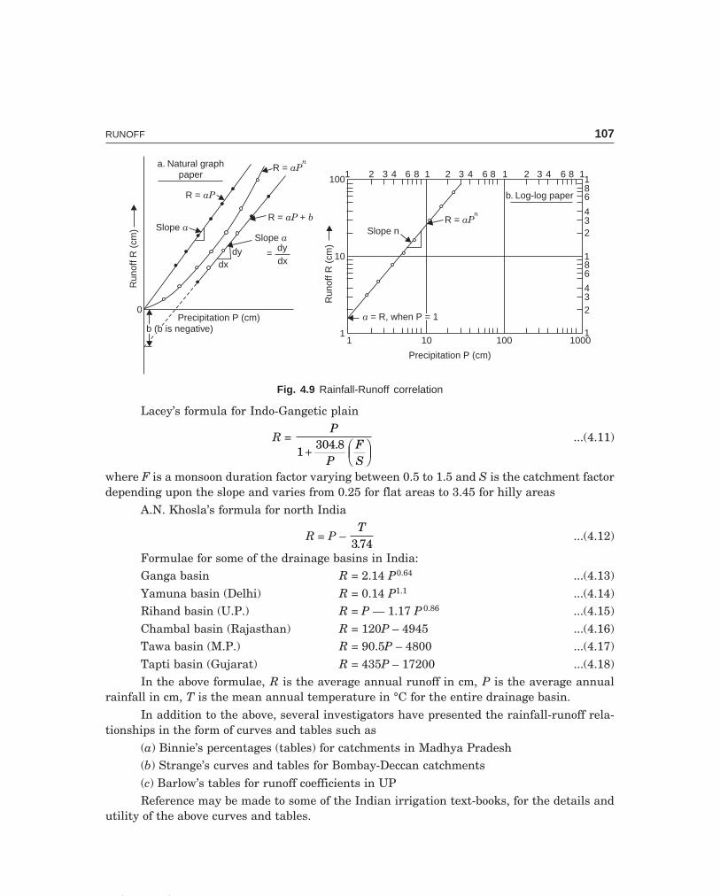
C-9\N-HYDRO\HYD4-1.PM5 107
RUNOFF 107
R = aPn
Slope n
a = R, when P = 1a = R, when P = 1
b. Log-log paper
Run
offR
(cm
)
100
10
11 10 100 1000
1
234
681
234
6811864321864321864321
Precipitation P (cm)
R = aP
Slope a
b (b is negative)b (b is negative)Precipitation P (cm)
R = +aP b
R = aPn
Run
off R
(cm
)
a. Natural graphpaper
0
Slope a
=dydx
dydx
Fig. 4.9 Rainfall-Runoff correlation
Lacey’s formula for Indo-Gangetic plain
R = P
PFS
1304 8+ F
HGIKJ
....(4.11)
where F is a monsoon duration factor varying between 0.5 to 1.5 and S is the catchment factordepending upon the slope and varies from 0.25 for flat areas to 3.45 for hilly areas
A.N. Khosla’s formula for north India
R = P – T
374....(4.12)
Formulae for some of the drainage basins in India:Ganga basin R = 2.14 P0.64 ...(4.13)Yamuna basin (Delhi) R = 0.14 P1.1 ...(4.14)Rihand basin (U.P.) R = P — 1.17 P 0.86 ...(4.15)Chambal basin (Rajasthan) R = 120P – 4945 ...(4.16)Tawa basin (M.P.) R = 90.5P – 4800 ...(4.17)Tapti basin (Gujarat) R = 435P – 17200 ...(4.18)In the above formulae, R is the average annual runoff in cm, P is the average annual
rainfall in cm, T is the mean annual temperature in °C for the entire drainage basin.In addition to the above, several investigators have presented the rainfall-runoff rela-
tionships in the form of curves and tables such as(a) Binnie’s percentages (tables) for catchments in Madhya Pradesh(b) Strange’s curves and tables for Bombay-Deccan catchments(c) Barlow’s tables for runoff coefficients in UPReference may be made to some of the Indian irrigation text-books, for the details and
utility of the above curves and tables.
C-9\N-HYDRO\HYD4-1.PM5 108
108 HYDROLOGY
The yield of a catchment can be simply worked out by taking about 75 to 80% of thea.a.r. and assuming a suitable runoff coefficient.
The rainfall of an average bad year ≈ 23 to 3
4 of the a.a.r., which may be taken for runoff
computation. Further improvement over the a.a.r. is the dependable rainfall. The availableannual rainfall records for about 35 years are arranged in the descending order and the rainfallof 75% dependability, i.e., of the 27th year from the top is taken for runoff computation.*
Several empirical formulae have also been developed for estimating the maximum rateof runoff or Maximum Flood Discharge (MFQ) and these are given under Chapter–8 on Floods.
(ii) Infiltration Method. By deducting the infiltration loss, i.e., the area under the infil-tration curve, from the total precipitation or by the use of infiltration indices, which are al-ready discussed. These methods are largely empirical and the derived values are applicableonly when the rainfall characteristics and the initial soil moisture conditions are identical tothose for which these are derived.
(iii) Rational Method. A rational approach is to obtain the yield of a catchment by as-suming a suitable runoff coefficient.
Yield = CAP ...(4.19)where A = area of catchment
P = precipitation C = runoff coefficientThe value of the runoff coefficient C varies depending upon the soil type, vegetation
geology etc. and the following Table 4.3 given by Richards may be taken as a guide.
Table 4.3 Runoff coefficients for various types of catchments
Type of catchment Value of C
Rocky and impermeable 0.8–1.0
Slightly permeable, bare 0.6–0.8
Cultivated or covered with vegetation 0.4–0.6
Cultivated absorbent soil 0.3–0.4
Sandy soil 0.2–0.3
Heavy forest 0.1–0.2
In the rational method, the drainage area is divided into a number of sub-areas andwith the known times of concentration for different subareas the runoff contribution fromeach area is determined. The choice of the value of the runoff coefficient C for the differentsub-areas is an important factor in the runoff computation by this method. This method ofdividing the area into different zones by drawing lines of time contour, i.e., isochrones, isillustrated in the following example.
*Frequency F = mn
× 100 ∴ 75% = m35
× 100 ∴ m = 27

C-9\N-HYDRO\HYD4-1.PM5 109
RUNOFF 109
Example 4.3 A 4-hour rain of average intensity 1 cm/hr falls over the fern leaf type catchmentas shown in Fig. 4.10. The time of concentration from the lines AA, BB, CC and DD are 1, 2, 3and 4 hours, respectively, to the site 0 where the discharge measurements are made. The valuesof the runoff coefficient C are 0.5, 0.6, and 0.7 for the 1st, 2nd and 3rd hours of rainfail respec-tively and attains a constant value of 0.8 after 3 hours. Determine the discharge at site 0.
Q
Dischargesite
I
IIIIIIV
20 ha
t=
1hr
c
t=
2hr
c
t=
3hr
ct=
4hr
c
40 ha 50 ha 30 ha
Catchmentarea
IsochronesBasinboundary
C
B
A
DD
C B
A
O
Fig. 4.10 Time of concentration method of runoff computation (Example 4.3)
Solution The discharge computations are made in Table 4.4.Example 4.4 The following data are collected for a proposed tank in the Deccan plains of southIndia:
Catchment area = 1200 ha
a.a.r. = 90 cmIntensity of rainfall of duration 1 hr
and frequency 35 years = 5 cm/hrAverage runoff cofficient for the
whole catchment = 20%
Tank gets filled = 1 12 times in a year
Difference between the maximum
water level (MWL) and full tanklevel (FTL) = 0.6 m
Determine(a) the yield of the catchment and the capacity of the tank
(b) the area of rice crop that can be irrigated from the tank(c) the duties of water assumed and the discharge at the head to the distributary
(d) the length of clear overfall weir near one flank.Solution A.A.R. is available only in 50% of the years. To ensure filler of the tank in deficientyears dependable rainfall ≈ 75% of a.a.r.
= 0.75 × 90 = 67.5 cm or 0.675 m.Corresponding to this rain (P) of 75% dependability, the runoff (R) can be found from
Eq. (4.10).

C-9\N-HYDRO\HYD4-1.PM5 110
110 HYDROLOGY
Su
b-ar
ea (
zon
e)T
ime
from
beg
inn
ing
of s
torm
(h
r)
con
trib
uti
ng
run
off
(ha)
12
34
56
78
I20
2020
20
II30
3030
30
III
5050
5050
IV40
4040
40—
Dis
char
ge a
t 0
from
su
b-ar
eas
0.5
(20
×0.
6 (2
0 ×
0.7
(20
×0.
8 (2
0 ×
—
Q =
ΣC
AP
104 )
1 100
104 )
1 100
104 )
1 100
104 )
1 100
0.5
(30
×0.
6 (3
0 ×
0.7
(30
×0.
8 (3
0 ×
—
104 )
1 100
104 )
1 100
104 )
1 100
104 )
1 100
0.5
(50
×0.
6 (5
0 ×
0.7
(50
×0.
8 (5
0 ×
—
104 )
1 100
104 )
1 100
104 )
1 100
104 )
1 100
0.5
(40
×0.
6 (4
0 ×
0.7
(40
×0.
8 (4
0 ×
—
104 )
1 100
104 )
1 100
104 )
1 100
104 )
1 100
Dis
char
ge a
t 0
1000
2700
5700
8700
8300
6800
3200
—
Q (
m3 /
hr)
Tab
le 4
.4 T
ime
of c
once
ntr
atio
n m
eth
od o
f ru
nof
f co
mpu
tati
on.
(Exa
mpl
e 4.
3)

C-9\N-HYDRO\HYD4-1.PM5 111
RUNOFF 111
R = ( . )P P− 17 8
254 =
( . . ) .67 5 17 8 67 5254
− = 13.2 cm
Since the runoff coefficient C = 20% (given) R = CP = 0.20 × 67.5 = 13.5 cm
which compares well with the value obtained above by applying the empirical formula for theregion.
Yield from the catchment = CAP = 0.2 × 1200 × 0.675 = 162 ha-m
Since the tank gets filled 1 12 times in a year,
Capacity of the tank = 16215.
= 108 ha-m
(b) Assuming loss of water due to evaporation and seepage as 10% in the tank and 20%in the distributary
Water available at the field outlet = 162 (1 – 0.3) = 113.4 ha-mFor rice crop assuming U = 88 cm, crop period B = 120 days
Field irrigation requirement ∆ = U
ηirrgn= 88
0 7.
= 126 cm or 1.26 m = 1.26 ha-m/haArea of rice crop that can be irrigated
= 113.4 h m
1.26 m−
= 90 ha
(c) Tank duty = 1 0 3126− ..
= 0.555 ha/ha-m of annual storage (i.e., yield)
For 1 Mm3: (1 0.3) 10 m
1.26 10 m / ha
6 3
4 2
−× = 55.5 ha/Mm3 of annual storage
Note: 162 × 0.555 = 90 haFlow duty (D) as ha/cumec on field can be obtained from equal volumes
1 msec
3 (B days × 86400 sec) = (D × 104 m2) ∆m
∴ D = 8 64. B
∆= ×8.64 120 days
1.26 m = 823 ha/cumec
Discharge at field outlet = 90823
= 0.1093 cumec
Discharge at the head of the distributary, i.e., tank outlet= 0.1093/0.80 = 0.137 cumec = 137 lps
(d) Length of the clear overfall weir (L):Using the rational formula for the maximum rate of runoff
Q = CiA = 0.2 5
100 60 60( )× (1200 ×104) = 33.3 cumec
Weir formula is Q = CLH3/2

C-9\N-HYDRO\HYD4-1.PM5 112
112 HYDROLOGY
Head over the weir H = MWL – FTL = 0.6 m, L = length of the weirAssuming a weir coefficient C of 1.84, the weir formula becomes∴ 33.3 = 1.84 L (0.6)3/2
∴ L = 39 mNote. This example helps to distinguish between the hydrologic design and the hydraulic design.
The hydrologic design consists of arriving at the minimum rate of runoff (yield) and maximum rate ofrunoff (flood) from a catchment, while the hydraulic design helps to design the storage capacity of thetank, the tank outlet, the outlet on the field, the design of the distributary (as open channel) and thelength of the clear overfall weir and other apurtenances (from the principles of hydraulic engineering).Similarly hydrologic studies are made to arrive at the design flood for a spillway or bridge, and thehydraulic design consists of computing the length of spillway (for a desired head over the spillway) orcalculating HFL, afflux and lineal water way for bridge openings, etc.
(iv) Overland Flow Hydrograph. Overland flow occurs as a thin sheet of water over theground surface (soon after a storm starts), joins a stream channel, and then flows in the chan-nel to the concentration point. Overland flow is relatively slow and is the dominant type offlow in the case of very small areas such as air ports, municipal block areas and flow frombroad surfaces into storm drains and gutters. But in the case of large drainage areas, thelength of overland flow is so short in comparison with the channel flow distance (before reachingthe concentration point) that the total concentration time is mainly a function of channel velocity.
Overland flow is essentially a uniform flow over the surface (Fig. 4.11) as developed byC.F. Izzard (1948). The Reynolds number
Re = Vd qν ν
= ...(4.20)
where V = velocity of flowd = uniform depth of flowν = kinematic viscosity of waterq = discharge per unit width
Watersheet
P1
y
t0
w sin a
P2
a
aW
DxDx Water surface
Land surface
+ slopes
�� �
F = 0 per unit width
P – P + w sin – ( x.1) = 0s
1 2 0t
Fig. 4.11 Laminar overland flow analysis (after C.F. Izzard, 1948)

C-9\N-HYDRO\HYD4-1.PM5 113
RUNOFF 113
Experiments indicate that the overland flow can be assumed to be laminar if Re ≤ 1000and turbulent if Re > 1000 with a transition region of uncertainity in the vicinity of Re = 1000.Izzard suggested that for rectangular drainage areas, laminar flow can be assumed if the
product inet × l >| 400, where inet is the net rainfall in cm/hr and l is the length of overland flowin metres. Finite difference methods, based upon the method of characteristics have also beenused to develop overland flow hydrographs.
(v) Unit Hydrograph Method. The hydrograph of direct surface discharge measured atthe outlet of drainage area, which produces a unit depth of direct runoff (i.e., a Pnet of 1 cm overthe entire area of the catchment) resulting from a unit storm of specified duration (called unitperiod) is called a unit hydrograph of that duration. The unit hydrograph method was firstproposed by L.K. Sherman in 1932. The area under the hydrograph represents a direct runoffof 1 cm, Fig. 4.12.
Time t (hr)
TRunoff duration (hr)
TRunoff duration (hr)
ttime of
concentration
cttime of
concentration
c
Unit hydrograph
Inflection point
Area under thecurve = runoffvolume of 1-cm depthover catchment
Dis
char
geQ
(cum
ec)
O
Inte
nsity
i(cm
/hr)
t2r
Qp
tptp
Basin lag (hr)
Peak, Qp
Time t (hr)
tr = duration of storm (i = 1/t cm/hr)r
cg of PnetP = net storm rain of 1 cmnet
Fig. 4.12 Unit hydrograph
The theory of unit hydrograph is based on the following assumptions:(i) The net rainfall is of uniform intensity within its duration (i.e., unit period).
(ii) The net rainfall uniformly occurs over the entire area of the drainage basin.(iii) For a given drainage basin, the base period of the hydrographs of direct runoff cor-
responding to net rains of different intensities but same unit duration, is constant.(iv) The ordinates of direct runoff hydrographs due to net rains of different intensities
(but same unit duration) are proportional.(v) A unit hydrograph reflects all the physical characteristicts of the basin.

C-9\N-HYDRO\HYD4-1.PM5 114
114 HYDROLOGY
Application of the Unit Hydrograph. First a unit hydrograph of suitable unit duration isderived from an observed flood hydrograph for the drainage basin due to a known storm (stormloss and net rain). The unit hydrograph so derived can be applied for any other storm (of thesame duration but producing different net rain) occurring on the basin and the resulting floodhydrographs can be obtained.
The details of the derivation of unit hydrographs and their application, given a unithydrograph of one duration to derive a unit hydrograph of some other duration, and derivationof unit hydrographs for meteorologically homogeneous catchments (i.e., from basincharacteristics like shape, size, slope etc. when the stream-outflows are not gauged) are givenin Chapter—5.
Example 4.5 A small watershed consists of 1.5 km2 of cultivated area (c = 0.2), 2.5 km2 underforest (c = 0.1) and 1 km2 under grass cover (c = 0.35). There is a fall of 20 m in a watercourse of
length 2 km. The I–D–F relation for the area is given by I = 80 T
(t 12)
0.2
0.5+, I in cm/hr, T–yr, t-min.
Estimate the peak rate of runoff for a 25-year frequency.
Solution Time of concentration (Kirpich’s formula–modified)tc ≈ 0.02 L0.8 S–0.4, tc in min, L in metres
= 0.02 (2000)0.8 20
2000
0.4FHG
IKJ
−
= 55 min = t
I = 80 2555 12
0.2
0.5
×+( )
= 18.6 cm/hr
Q = CIA = 2.78 I (Σ Ci Ai) = 2.78 × 18.6 (1.5 × 0.2 + 2.5 × 0.1 + 1 × 0.35) = 46.5 Cumec
�������
I Match the items in ‘A’ with the items in ‘B’
A B(i) Isochrone (a) C.F. Izzard
(ii) Runoff coefficient (b) Topographic ridge
(iii) Unit hydrograph (c) Arid region
(iv) Compactness coefficient (d) Perennial streams
(v) Effluent streams (e) Shape of drainage basin
(vi) Ephemeral streams (f) 1 cm of runoff
(vii) Drainage divide (g) Yield of catchment
(viii) Overland flow hydrograph (h) Time-contours of commencement of storm
II Say ‘true’ or ‘false’ if false, give the correct statement.
(i) Direct runoff is the sum of overland flow and interflow.
(ii) In a perennial stream the ground water table is always below the bed of the stream while theground water table is always above the bed in an ephemeral stream.

C-9\N-HYDRO\HYD4-1.PM5 115
RUNOFF 115
(iii) Bank storage is the portion of runoff stored in the permeable banks of a stream due to arising flood.
(iv) The drainage density varies directly as the length of overland flow and indicates the drain-age efficiency of the basin.
(v) Quick intense floods occur more in fern-shaped catchments than in fan-shaped catchments.
(vi) For the same intensity of rainfall, the flood discharge from a relatively small catchment ishigher than that from a relatively large catchment.
(vii) Vegetation tends to increase the runoff from the catchment. (false: ii, iv, v, vii)
III Choose the correct statement/s in the following:
1 Maximum surface runoff is favoured due to
(i) presence of forest area
(ii) a flash storm
(iii) presence of a recharge area, which replenishes the ground water storage
(iv) leaf-shaped catchment
(v) fan-shaped catchment
(vi) storm movement opposite to the stream flow
(vii) humid climate
(viii) improved land management
2 An influent stream is due to
(i) a river crossing a desert area
(ii) effluent seepage from the basin
(iii) ground water table being above the stream bed
(iv) base flow
(v) direct surface runoff
(vi) being ephemeral in nature (1–ii, v, vii; 2—i, v, vi)
�������
1 Name three forms in which water is stored on a catchment.
2 What is meant by ‘the water balance of a catchment’?
3 Dicuss the various factors, which affect the runoff from a basin.
4 (a) What are the methods of estimating runoff from a catchment?
(b) Give three empirical formulae applicable to particular regions in India.
5 How do you determine the yield from a catchment and arrive at the capacity of a tank?
6 Differentiate: Runoff, yield and maximum flood discharge.
7 Determine the yield of the catchment and the capacity of the tank from the following data:
Catchment area = 20 km2
a.a.r. = 80 cm
Tank gets filled: 2 times in a year
Runoff coefficient = 15
(average for the catchment) (2, 4, 1.2 Mm3)

C-9\N-HYDRO\HYD4-1.PM5 116
116 HYDROLOGY
8 Explain the terms: catchment area and drainage divide.
An irrigation tank has a catchment area of 30 km2 and receives an annual rainfall of 90 cm.Assuming that 10% of the rainfall flows as ‘runoff’ from the catchment, calculate the area thatcan be brought under paddy cultivation under the tank. Assume that the tank fills one and a halftimes in a year and the water requirement of paddy (duty) is 100 ha-cm. (40.5 ha)
9 (a) Explain how the following physical characteristics of a catchment can be determined?
(i) Mean elevation
(ii) Mean slope
(b) Krishna River basin has an area of 258948 km2 and length 1400 km. Calculate the formfactor and elongation ratio. (0.132, 0.41)
10 Explain the terms: Catchment area, Drainage divide, and Ground water divide. An irrigationtank has a catchment area of 30 km2 and the a.a.r. is 90 cm. Assuming that only 20% of thedependable rainfall is the runoff available. Calculate the capacity of the tank assuming that itfills one and a half times in a year.
Assuming a total depth of irrigation water for rice crop for 120 days as 1.25 m and 30% losses,what area of rice crop can come under the tank?
Work out the tank duty, field duty and the discharge required at the tank outlet.
What is the length of the clear overfall weir to dispose of flood waters, assuming an intensity of5 cm/hr of 35-year frequency. (270 ha-m, 227 ha, 56 ha/Mm3, 828 ha/cumec, 343 lps, 97.5 m)
11 A catchment has a perimeter of 1020 km and an area of 38520 km2. Calculate the compactnesscoefficient.
12 Write short notes on
(i) Isochrones (ii) Ephemeral streams
(iii) Time of concentration (iv) Overland flow hydrograph
(v) Runoff cycle (vi) Valley storage
(vii) Bank storage
13 Distinguish between
(i) Overland flow and interflow (ii) Influent and effluent streams
(iii) Detention storage and depression storage
(iv) Drainage density and drainage divide
(v) Form factor and compactness coefficient of a catchment
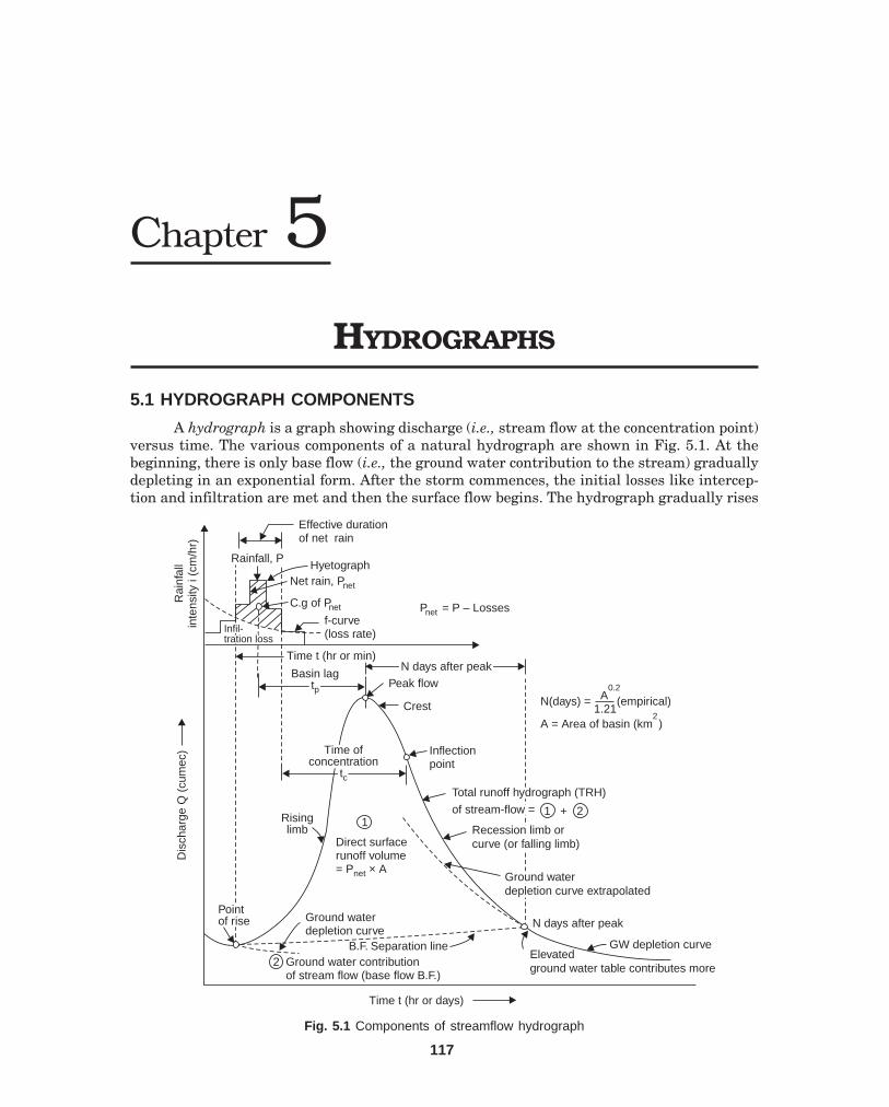
5.1 HYDROGRAPH COMPONENTS
A hydrograph is a graph showing discharge (i.e., stream flow at the concentration point)versus time. The various components of a natural hydrograph are shown in Fig. 5.1. At thebeginning, there is only base flow (i.e., the ground water contribution to the stream) graduallydepleting in an exponential form. After the storm commences, the initial losses like intercep-tion and infiltration are met and then the surface flow begins. The hydrograph gradually rises
Effective durationof net rain
Rainfall, P
Net rain, Pnet
C.g of Pnet
f-curve(loss rate)Infil-
tration lossInfil-tration loss
Rai
nfal
lin
tens
ityi (
cm/h
r)D
isch
arge
Q(c
umec
)
Time t (hr or days)
B.F. Separation lineGround water contributionof stream flow (base flow B.F.)
2
Ground waterdepletion curve
Pointof risePointof rise
Risinglimb
Direct surfacerunoff volume= P × Anet
1
Time ofconcentration
tc
Time ofconcentration
tc
Inflectionpoint
Basin lagtp
Basin lagtp
Pnet = P – Losses
N days after peakN days after peak
Peak flow
Crest
Total runoff hydrograph (TRH)
of stream-flow =
Total runoff hydrograph (TRH)
of stream-flow = 1 + 21 + 2
Recession limb orcurve (or falling limb)Recession limb orcurve (or falling limb)
Ground waterdepletion curve extrapolatedGround waterdepletion curve extrapolated
Elevatedground water table contributes more
GW depletion curve
N days after peak
N(days) = (empirical)
A = Area of basin (km2)
A1.21
0.2
Time t (hr or min)Time t (hr or min)
Hyetograph
Fig. 5.1 Components of streamflow hydrograph
Chapter 5
117
HYDROGRAPHS

C-9\N-HYDRO\HYD5-1.PM5 118
118 HYDROLOGY
and reaches its peak value after a time tp (called lag time or basin lag) meaured from thecontroid of the hyetograph of net rain. Thereafter it declines and there is a change of slope atthe inflection point, i.e., there has been, inflow of the rain up to this point and after this thereis gradual withdrawal of catchment storage. By this time the ground water table has beenbuilt up by the infiltrating and percolating water, and now the ground water contributes moreinto the stream flow than at the beginning of storm, but thereafter the GWT declines and thehydrograph again goes on depleting in the exponential form called the ground water depletioncurve or the recession curve. If a second storm occurs now, again the hydrograph starts risingtill it reaches the new peak and then falls and the ground water recession begins, Fig. 5.2.
Storm 1 Storm 2Storm 3
Pnet1Pnet2
Pnet3
Loss Loss Loss
3 peaks due to3-storms insuccession
Recessionlines
Estimated base flow
Time t (hr or days)
Dis
char
geQ
(cum
ec)
Inte
nsity
i (cm
/hr)
Fig. 5.2 Hydrograph with multiple peaks
Thus, in actual streams gauged, the hydrograph may have a single peak or multiplepeaks according to the complexity of storms. For flood analysis and derivation of unithydrograph, a single peaked hydrograph is preferred. A complex hydrograph, however, can beresolved into simple hydrographs by drawing hypothetical recession lines as shown in Fig. 5.2.
It has been found from many hydrographs that the ground water depletion curves for agiven drainage basin are nearly the same and hence it is termed as the normal ground waterdepletion curve. It has been found that such curves, or at least their segments, follow a simpleinverse exponential function of the elapsed time of the form.
Qt = Q0 Kr–t ...(5.1)
where Q0 = discharge at start of periodQt = discharge at end of time tKr = recession constant
As Qt is the derivations of storage with respect to time,– d St = Qt dt

C-9\N-HYDRO\HYD5-1.PM5 119
HYDROGRAPHS 119
∴ St = – z Qt dt = – z (Q0 Kr–1) dt
∴ St = Q
Kt
e rlog� z ax =
aa
x
log...(5.2)
Hence, the discharge at any time is proportional to the water remaining in storage i.e.,
QQt
0 =
SSt
0...(5.2 a)
Taking logarithms on both sides of Eq. (5.1)log Qt = log Q0 – t log Kr
which is in the straight line form y = mx + c with y = log Qt, x = t, and m = – log Kr. The valueof Kr can be determined by plotting the recession data i.e., Qt vs. t on a semi-log paper, takingcare to select periods of little or no direct runoff; see Example 17.3.
Time t (hr or days) (natural scale)
Dis
char
geQ
(cum
ec)
Log
scal
e
a. Semi-log plot of continuousdischarge hydrograph
Masterdepletion curve(semi-log plot)
a
b
ce
gd
f
b. Semi-log plot ofmaster depletion curve
Lower ends of curvesare tangential to acommon line
i
jh
Time t (hr or days) (natural scale)
Log
Q
Master depletioncurve (natural scale)
c. Master depletioncurve drawn to linear scale
Time t (hr or days)
Dis
char
geQ
(cum
ec)
a
b
c
d
e
f
g
h i
Fig. 5.3 Composite ground water depletion curve

C-9\N-HYDRO\HYD5-1.PM5 120
120 HYDROLOGY
If a continuous stream flow record is available for a number of years, the hydrographcan be plotted on a semi-log paper, i.e., log Q vs. t, Fig. 5.3. Starting with the lowest recessionflow line, a line is drawn tangential to the lower portion on a tracing paper. This tangent lineis progressively extended by moving the tracing-paper towards the origin with the abscissaecoincident, such that the line is tangential to the lower portion of the successive depletioncurves of increasing magnitude. This common line is the log plot of the master depletion curve,which is then converted to linear vertical scale and is called the composite ground water depletioncurve.
A composite ground water depletion curve can be constructed from the recession graphsresulting from a number of storms. The various segments of the recession graphs are shiftedwith respect to the time axis until they appear to match and then, an average or compositecurve is drawn through them as shown in Fig. 5.4.
20
18
16
14
12
10
8
6
4
2
03 6 9 12 15 18 21 24 27
Time t (hr or days)
Dis
char
geQ
(cum
ec10
or10
0)
Master depletion curve
Storm recession curvesmoved (to match) w.r.t.time-axis
Fig. 5.4 Composite depletion curve
5.2 SEPARATION OF STREAMFLOW COMPONENTS
Barnes (1940) proposed that the stream flow components may be separated by plotting thehydrograph on a semi-log paper (Fig. 5.5). The tail end of the hydrograph plots as a straightline, i.e., ground water recession (CD). If this straight line plot is extended backwards up to thepoint E directly under the inflection point I and line BE drawn, the area under BEC representsthe ground water contribution to the stream flow. If the ordinates of this area are deductedfrom the ordinates of the total hydrograph and replotted, the hydrograph of surface runoff andinterflow (subsurface flow) is obtained, which plots as a straight line (HG) at the tail end. Byextending this line backwards up to the point L directly under I and drawing the line FL, thearea under FLG gives the interflow component. By deducting the ordinates of this from theordinates of the hydrograph of surface runoff and interflow, the hydrograph of surface runoffis replotted whose tail end again, may plot as a straight line representing the surface recession

C-9\N-HYDRO\HYD5-1.PM5 121
HYDROGRAPHS 121
or channel storage. The slopes of the straight line plots at the tail ends of the separatedhydrographs give the respective recession constants.Example 5.1 The mean daily streamflow data from a drainage basin is given below. It is knownthat the recession limb of the discharge hydrograph has components of channel storage, interflowand base flow. Find the values of the recession coefficients for each of the three components.
Date Mean daily discharge Date Mean daily discharge(cumec) (cumec)
1978, Oct. 4 278 1978, Oct. 14 179
5 265 15 167
6 5350 16 157
7 8150 17 147
8 6580 18 139
9 1540 19 131
10 505 20 123
11 280 21 117
12 219 22 111
13 195 23 105
24 100
Also determine
(a) ground water storage on October 14, 1978.(b) ground water storage and stream flow on October 30, 1978, assuming no rainfall
during the period.Solution The discharge hydrograph is drawn on a semi-log paper and the flow componentsare separated by the method proposed by Bernes as shown in Fig. 5.5. The recession coeffi-cients (Kr) for the three components of base flow (ground water contribution), interflow andchannel storage are computed as 1.059, 2.104 and 4.645, respectively.
(a) Ground water storage (S0) on October 14, 1978 when the ground water depletionstarts.
S0 = Q
ke r
0
log= ×179 86400 m /day
log 1.06/day
3
e = 2.75 × 10⁸ m3
(b) Stream flow on October 30, 1978, i.e., after 16 daysQt = Q0 Kr
–t
Q16 days = 179 (1.06)–16 = 71.6 cumecGround water storage (St) on October 30, 1978 can be determined from
QQt
0 = SSt
0
or St = S0 × QQ
t
0
∴ S16 days = (2.75 × 10⁸) 716179
. = 1.10 × 10⁸ m3

C-9\N-HYDRO\HYD5-1.PM5 122
122 HYDROLOGY
100008
6
4
3
2
10008
6
4
3
2
1008
654
3
2
108
6543
2
110 11 12 13 14 15 16 17 18 19 20 21 22 23 24 25 26 27 28 29 30
Interflow
Surfacerecession
Surfacerunoff
Semi-log paper
Total runoff hydrograph(of stream flow)
Q = Q Kt o r–t
Log Q = log Q – t log Kt o rüýþ üýþ üýþy c m+ x (Slope m is –ve)
m = – log K , K = daily depletion factoror recession constant
r r
Surface runoff plus interflow
Ground water recession
–m = = 0.026= log Kr
log 330/10020 days
K = 1.06 daysr–1
K=
2.10days
r
–1
K=
4.64days
r
–1
H
GM
Date Days – Natural scale
F
E
LL
C
I
BA
Log-
scal
eD
isch
arge
Q(c
umec
)
D
Fig. 5.5 Separation of streamflow components (after Barnes, 1940)
5.3 HYDROGRAPH SEPARATION
For the derivation of unit hydrograph, the base flow has to be separated from the total runoffhydrograph (i.e., from the hydrograph of the gauged stream flow). Some of the well-knownbase flow separation procedures are given below, Fig. 5.6.
(i) Simply by drawing a line AC tangential to both the limbs at their lower portion.This method is very simple but is approximate and can be used only for preliminary estimates.
(ii) Extending the recession curve existing prior to the occurrence of the storm up to thepoint D directly under the peak of the hydrograph and then drawing a straight line DE, whereE is a point on the hydrograph N days after the peak, and N (in days) is given by
N = 0.83 A0.2 ...(5.3)

C-9\N-HYDRO\HYD5-1.PM5 123
HYDROGRAPHS 123
PeakB
N days
I
Directsurfacerunoff
Directsurfacerunoff
4
2
32
1
Time t (hr or days)
Dis
char
geQ
(cum
ec)
N (days) = 0.84 A (empirical)
A = Drainage area (km
0.2
2)
Four separation procedures
E (N days after peak)G
C Recession
Ground water contributionto stream (base flow)D
FPoint ofriseA
Fig. 5.6 Hydrograph separation
where A = area of the drainage basin, km2 and the size of the areas of the drainage basin as aguide for the values of N are given below :
Area of drainage basin (km2) 250 1250 5000 12500 25000
Time after peak, N (days) 2 3 4 5 6
(iii) Simply by drawing a straight line AE, from the point of rise to the point E, on thehydrograph, N days after the peak.
(iv) Construct a line AFG by projecting backwards the ground water recession curveafter the storm, to a point F directly under the inflection point of the falling limb and sketch anarbitrary rising line from the point of rise of the hydrograph to connect with the projected baseflow recession. This type of separation is preferred where the ground water storage is rela-tively large and reaches the stream fairly repidly, as in lime-stone terrains.
Many a time a straight line AE meets the requirements for practical purposes. Locationof the point E is where the slope of the recession curve changes abruptly, and as a rough guideE is N days after the peak. In all the above four separation procedures, the area below the lineconstructed represents the base flow, i.e., the ground water contribution to stream flow. Anyfurther refinement in the base flow separation procedure may not be needed, since the baseflow forms a very insignificant part of high floods. In fact, very often, a constant value of baseflow is assumed.
In Fig. 5.7, ADE is the assumed base flow. Actually, when the water level in the streamrises due to floods, the stream feeds the ground water and the permeable boundaries (calledbank storage, Fig. 5.8) and this is termed as negative base flow. But actually the variation inbase flow may be much less than indicated in Fig. 5.7 depending on the permeability of theboundaries and the gradient of the phreatic surface. The resulting variation will be a slight dipfrom the extrapolated depletion curve, followed by a gradual rise to a higher level than theinitial value as the flood recedes as shown in Fig. 5.9.

C-9\N-HYDRO\HYD5-1.PM5 124
124 HYDROLOGY
Time t (hr) Negative base flow(bank storage)
Increase in base flowafter flood
Dischargehydrograph
Surfacerunoff
Recessioncurves
Dis
char
geQ
(cum
ec)
A
E
D
Fig. 5.7 Negative baseflow
GWT
Ground water flowGround water flow(during low water period)
Permeablebanks of stream
GWT
Bank storage
High water level
Low water level
Fig. 5.8 Bank storage
DischargehydrographDirect
surfacerunoff
Separation line
Extrapolateddepletion curve
Base flow
Recessioncurve
Time t (hr)
Dis
char
geQ
(cum
ec)
Fig. 5.9 Actual baseflow variation
5.4 UNIT HYDROGRAPH
The unit hydrograph is defined as the hydrograph of storm runoff resulting from an isolatedrainfall of some unit duration occurring uniformly over the entire area of the catchment, pro-duces a unit volume (i.e., 1 cm) of runoff.
Derivation of the unit hydrographs. The following steps are adopted to derive a unithydrogaph from an observed flood hydrograph (Fig. 5.10).

C-9\N-HYDRO\HYD5-1.PM5 125
HYDROGRAPHS 125
4646 4545 4545 4545 4646 4848 5050 5353 5454 5757 6060 5555 5151 5050
300
250
200
150
100
50
02 5 8 11 14 17 20 23 2 5 8 11 14 17 20 23
10
8
6
4
2
00 3 6 9 12 15 18 21 24 27 30 33
Rai
nfal
lin
tens
ityi (
cm/h
r)Rainfall, P
P = 26.6 cm = Runoffnetc.g. of Pnet
f-index
Dis
char
ge(S
trea
mflo
w)
Q(c
umec
)
Time t (min)t = 3 hr = Effective duration of stormr
t = 10 hrp12
Basin lag
peak flowN = 0.84 (40) = 1 day (too long)
0.2 34
P = =netSQ .t
Ad 986 (3 × 60 × 60)
40 × 106
m
m
3
2
= 0.266 mor 26.6 cm ... 1
Totalrun offhydrograph
S SQ = DRO = 986 cumecd
P = P – Losses
= (i – )t ... 2net
S �t = duration of rain (min)
for which i > f P from 1 & 2should balanceDSR stops recession
net
Direct surfacerunoff = 26.6 cmDirect surfacerunoff = 26.6 cm
120 = TRO = Q120 = TRO = Q75 = DRO = TRO – BFO
= Q = 120 – 45d
75 = DRO = TRO – BFO= Q = 120 – 45dPoint of
risePoint of
rise D.SRstarts Arbitrary line of separation
Arbitrary line of separation
4747BFOBFO Base flowBase flow
1–3–19701–3–1970 2–3–19702–3–1970
Dis
char
ge–
cum
ec
Hours from beginning of runoff
Runoff duration T = 32 hrRunoff duration T = 32 hr
P =
1 cmnet
t2r
tr 75/2
6.6
=2.
8275
/26.
6=
2.82
tptp
Date and time hrPeak of UG
Unithydrograph
Area undercurve = 1 cmof runoff
2.82 = UGO = DROPnet
TRO – BFO = DROTRO – BFO = DRO
= UGO (for which P = 1 cm)net= UGO (for which P = 1 cm)netDROPnet
t = 3 hr = unit hydrograph durationrt = 3 hr = unit hydrograph durationr
Time to peak = t +pTime to peak = t +p
Recession
tr2tr2
Fig. 5.10 Derivation of a unit hydrograph (Example 5.1)
(i) Select from the records isolated (single-peaked) intense storms, which occurringuniformly over the catchment have produced flood hydrographs with appreciable runoff (>1cm, say, 8 to 16 cm). The unit period selected should be such that the excess rainfall (i.e., Pnet)occurs fairly uniformly over the entire drainage basin. Larger unit periods are required forlarger basins. The unit periods may be in the range of 15-30% of the ‘peak time’ period, i.e., thetime from the beginning of surface runoff to the peak, and the typical unit periods may be 3, 6,8, 12 hours. (The time of concentration may be a little longer than the peak time).
C-9\N-HYDRO\HYD5-1.PM5 126
126 HYDROLOGY
The unit storm is a storm of such duration that the period of surface runoff is not muchless for any other storm of shorter duration.
(ii) Select a flood hydrograph, which has resulted from a unit storm chosen in item (i)above.
(iii) Separate the base flow from the total runoff (by the well-known base flow separa-tion procedures).
(iv) From the ordinates of the total runoff hydrograph (at regular time intervals) deductthe corresponding ordinates of base flow, to obtain the ordinates of direct runoff.
(v) Divide the volume of direct runoff by the area of the drainage basin to obtain the netprecipitation depth over the basin.
(vi) Divide each of the ordinates of direct runoff by the net precipitation depth to obtainthe ordinates of the unit hydrograph.
(vii) Plot the ordinates of the unit hydrograph against time since the beginning of directrunoff. This will give the unit hydrograph for the basin, for the duration of the unit storm(producing the flood hydrograph) selected in item (i) above.
In unit hydrograph derivation, such storms should be selected for which reliable rain-fall and runoff data are available. The net rain graph (hyetograph of excess rain) should bedetermined by deducting the storm loss and adjusting such that the total volume of net stormrain is equal to the total volume of direct surface runoff. The unit hydrograph derived, which,when applied to the known net rain data, should yield the known direct runoff hydrograph.
The steps given above for the derivation of unit hydrograph can be formulated as fol-lows (exemplified in Fig. 5.10).
Pnet = P – Losses ...(5.4)
or Pnet = ΣQ t
Ad , Qd = DRO ...(5.4 a)
TRO—BFO = DRO ...(5.4 b)
DROPnet
= UGO ...(5.4 c)
where P = total rainfallPnet = net precipitation (from hyetograph) or direct runoff as equivalent depth
over the basin.Losses = due to infiltration (Fp), etc.
A = area of the drainage basinQd, DRO = direct runoff ordinate
TRO = total runoff ordinatet = time interval between successive direct runoff ordinates
BFO = base flow ordinateElements of unit hydrograph. The various elements of a unit hydrograph are shown in
Fig. 5.11.Base width (T)—The period of direct surface runoff (due to a unit storm) of the unit
hydrograph is called the time base or the base width.

C-9\N-HYDRO\HYD5-1.PM5 127
HYDROGRAPHS 127
Unitperiodtr
Unitperiodtr
Rai
nfal
lin
tens
ityi
i = cm/hr1tr
P = 1 cm = i × tnet r
Recession time TrRecession time TrLag time
tp
Lag timetp
t /2rtr/2Qp
Dis
char
geQ
(cum
ec)
Peak of UG, Q cumecp
Time to peakConcen-
tration timetc
Concen-tration time
tc
I, inflectionpoint
Unithydrograph
Channelstorage
Area undercurve1 cm of
runoff overcatchment
area A
º
Time base T (hr)Time base T (hr)
(Runoff duration)
Time t (hr)
Fig. 5.11 Elements of unit hydrograph
Unit storm—The strom of unit duration (i.e., duration of the unit hydrograph) regard-less of its intensity is called unit storm.
Unit period—The time duration of the unit storm (i.e., the duration of the unithydrograph) is called unit period.
Lag time (tp)—The time from the centre of a unit storm to the peak discharge of thecorresponding unit hydrograph is called lag time.
Recession time (Tr)—The duration of the direct surface runoff after the end of the excessor net rainfall, is called recession time in hydrograph analysis.
Propositions of the Unit HydrographThe following are the basic propositions of the unit hydrograph:
(i) Same runoff duration. For all unit storms of different intensities, the period of sur-face runoff (i.e., time base, base width or base period) is approximately the same, althoughthey produce different runoff volumes (Fig. 5.12 (a)).
(ii) Proportional ordinates. For unit storms of different intensities, the ordinates of thehydrograph at any given time, are in the same proportion as the rainfall intensities(Fig. 5.12 (a)).
(iii) Principle of superposition. If there is a continuous storm and/or isolated storms ofuniform intensity net rain, they may be divided into unit storms and hydrographs of runoff foreach storm obtained, and the ordinates added with the appropriate time lag to get the com-bined hydrograph (Fig. 5.12 (b)).

C-9\N-HYDRO\HYD5-1.PM5 128
128 HYDROLOGY
Inte
nsity
(cm
/hr)
xii
i = , xi = cm/hr1tr
xtr × t = 1 cmr
1tr
× t = x cmrxtr
Pnet
x cm1 cm
üýþ
tr
x Qp
Qpx Qy
Qy
Dis
char
geQ
(cum
ec)
Time base TTime base T
Time t (hr)
Run off= x cmRun off= x cm
QRun off= 1 cm
pQRun off= 1 cm
p
QyQy
t1t1 tpeak
Hydrograph (producesx cm of runoff)
Peaks occurat same time
Proportional ordinates
t – hr UG (1-cm runoff)r
Same time base T
(a) Proportional ordinates and same time base
Rai
nfal
lin
tens
ityi t = 2 tR r
x cm22
y cm
trtr
Continuous storm split into two unit storms
33z cm
Dis
char
geQ
(cum
ec)
Combined hydrograph (obtainedby summing the ordinates of thethree component hydrographs: 1, 2 & 3)
Hydrographscorrespondingto storm 1, 2 & 3
UGO × z
321
UGO × y
UGO × x
t – hr UGOrt – hr UGOr
Time t (hr)
(b) Principle of superposition
11
trP due to 3-storms
unit period t – hrnet
r
Fig. 5.12 Propositions of unit hydrograph
(iv) Same distribution percentages. If the total period of surface runoff (i.e., time base orbase width) is divided into equal time intervals the percentage of surface runoff that occursduring each of these periods will be same for all unit storms of different intensities (Fig. 5.13).

C-9\N-HYDRO\HYD5-1.PM5 129
HYDROGRAPHS 129
1 2 3 4 5 6 7 8 9 10
12
11
10
9
8
7
6
5
4
3
2
1
0
Rai
nfal
lin
tens
ityi (
cm/h
r)Pnet
y cm = i = cm/hrytr
x cm = i = cm/hrxtr
1 cm = i = cm/hr1tr
S Mid–ordinates of unit periods= 0.5 + 2.0 + 4.7 + 7.1 + 5.6+ 3.5 + 2.5 + 1.6 + 0.9 + 0.3= 28.7 units% of runoff in unit period 1
= × 100 = 1.74 2 (rounded)
and like that.
»0.528.7
UGO × y = y cm runoff hydrograph
UGO × x = x cm runoff hydrograph
Distribution percentages(Same for all units storms)
UGO = 1 cm runoff unit hydrograph
Area under UG = Area under bar graph
Mid-ordinates of unit periods
Bernard’s distribution graph
If t = 4 hr, T = 40 hrr
1%
3%5.5%5.5%
9%9%
12%12%
19.5%19.5%
25%25%
Unit period
25% runoffoccursin unitperiod 4
425%
316% 19.5
%
5
16%16%+
+ ve & – veareasshouldbalance
7.1 units7.1 units
5.65.6
3.53.5
2.52.51.61.6
0.90.9
UGO(1 cm)
UGO(1 cm)4.74.7
2.0 units2.0 units
7%7%
2%2%0.50.5
Time base T divided into 10 unit periodsTime base T divided into 10 unit periodsTime t (hr)
Dis
char
geQ
(cum
ec)
(say
, 10
cum
ecun
its)
–
Fig. 5.13 Distribution percentages same for all unit storms
Limitation of the Unit Hydrograph. Certain limitations are inherent in the unithydrograph theory. The runoff hydrograph reflects the combined effects of rainfall factors,loss factors and physiographic factors. The design storm continuing for several unit periodsmay not have the same areal distribution for each time increment. Storm movements alsoaffect the proportions of the unit hydrograph if the basin is large. Hence, the unit hydrographcan not be applied for basins larger than 5000 km2. For basins larger than 5000 km2, unithydrographs for the principal sub-areas or sub-basins are developed and the hydrographs ofrunoff determined for each sub-area. These hydrographs are then combined, through floodrouting procedure, to get the resulting hydrograph at the required section.
Derivation of Unit HydrographExample 5.1 (a) The runoff data at a stream gauging station for a flood are given below. Thedrainage area is 40 km2. The duration of rainfall is 3 hours. Derive the 3-hour unit hydrographfor the basin and plot the same.

C-9\N-HYDRO\HYD5-1.PM5 130
130 HYDROLOGY
Date Time Discharge Remarks(hr) (cumec)
1-3-1970 2 50
5 47
8 75
11 120
14 225
17 290 ← Peak
20 270
23 145
2-3-1970 2 110
5 90
8 80
11 70
14 60
17 55
20 51
23 50
State the peak of the unit hydrograph you derive.
Solution See Table 5.1.
5.5 UNIT HYDROGRAPH FROM COMPLEX STORMS
Unit hydrographs from complex storms, involving varying intensities of rain can be obtainedby considering the complex storm as successive unit storms of different intensities and therunoff hydrograph (due to complex storm) as the result of superposition of the successivestorm hydrographs. The ordinates of each storm hydrograph are obtained as ‘the storm inten-sity times the corresponding ordinate of the unit hydrograph’ as shown in Fig. 5.14. The unithydrograph ordinates u1, u2, ... are thus obtained by writing a series of equations for each ofthe ordinates Q1, Q2, .... of the runoff hydrograph (due to complex storm) and successivelysolving them. In Fig. 5.14,
Q1 = xu1 ∴ u1 = ?
Q2 = xu2 + yu1 ∴ u2 = ?
Q3 = xu3 + yu2 + zu1 ∴ u3 = ?
and so on. Thus, the tr–hour unit graph ordinates can be determined. Although the method isstraight forward, errors will creep in due to the assumptions on the intensity and duration ofrainfall and deduction of an assumed base flow; many trials are required to get a reasonableunit graph.
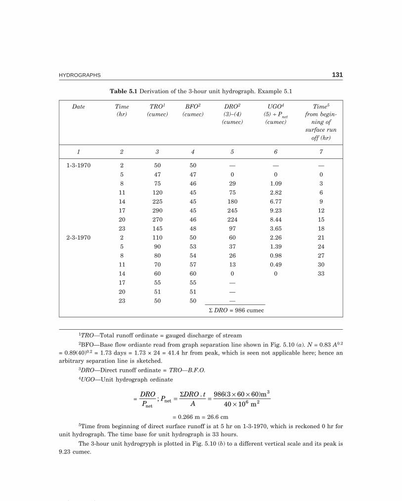
C-9\N-HYDRO\HYD5-1.PM5 131
HYDROGRAPHS 131
Table 5.1 Derivation of the 3-hour unit hydrograph. Example 5.1
Date Time TRO1 BFO2 DRO2 UGO4 Time5
(hr) (cumec) (cumec) (3)–(4) (5) ÷ Pnet from begin-(cumec) (cumec) ning of
surface runoff (hr)
1 2 3 4 5 6 7
1-3-1970 2 50 50 — — —
5 47 47 0 0 0
8 75 46 29 1.09 3
11 120 45 75 2.82 6
14 225 45 180 6.77 9
17 290 45 245 9.23 12
20 270 46 224 8.44 15
23 145 48 97 3.65 18
2-3-1970 2 110 50 60 2.26 21
5 90 53 37 1.39 24
8 80 54 26 0.98 27
11 70 57 13 0.49 30
14 60 60 0 0 33
17 55 55 —
20 51 51 —
23 50 50 —
Σ DRO = 986 cumec
1TRO—Total runoff ordinate = gauged discharge of stream2BFO—Base flow ordiante read from graph separation line shown in Fig. 5.10 (a). N = 0.83 A0.2
= 0.89(40)0.2 = 1.73 days = 1.73 × 24 = 41.4 hr from peak, which is seen not applicable here; hence anarbitrary separation line is sketched.
3DRO—Direct runoff ordinate = TRO—B.F.O.4UGO—Unit hydrograph ordinate
= DROP
PDRO t
Anetnet
3
6 2
986(3 60 60)m40 10 m
;.
= = × ××
Σ
= 0.266 m = 26.6 cm5Time from beginning of direct surface runoff is at 5 hr on 1-3-1970, which is reckoned 0 hr for
unit hydrograph. The time base for unit hydrograph is 33 hours.
The 3-hour unit hydrogryph is plotted in Fig. 5.10 (b) to a different vertical scale and its peak is9.23 cumec.

C-9\N-HYDRO\HYD5-1.PM5 132
132 HYDROLOGY
P due to 3-stormsnets
z cmz cmx cmx cmy cmy cm
trtr trtr trtr
Rai
nfal
lin
tens
ityi (
cm/h
r)
Dis
char
geQ
(cum
ec)
Q3
Q2
Q4
Q5Q1
yu 1
yu 1
zu 1
zu 1
yu 2
yu 2 zu 2
zu 2
Q6
Q7
00
xu 1
xu 1
yu 3
yu 3 zu 3
zu 3
u2u2u1u1 u3u3
xu 2
xu 2
t – hrUGOrt – hrUGOr
xu 4
xu 4
u4u4usus y u5y u5
z u4z u4
Time t (hr)00
0 z u5z u5
Observed hydrograph
Q = x u1 1
2 2 1
3 3 2 1
Q = x u + y uQ = x u + y u + z u , etc
Successively solvefor u , u , u , etc.which give t – hr UGO
1 2 3
ry
u 4y
u 4
x u5x u5
UGUGx u3x u3
Fig. 5.14 Derivation of unit hydrograph from multi-period storms
Example 5.2 The stream flows due to three successive storms of 2.9, 4.9 and 3.9 cm of 6 hoursduration each on a basin are given below. The area of the basin is 118.8 km2. Assuming aconstant base flow of 20 cumec, derive a 6-hour unit hydrograph for the basin. An averagestorm loss of 0.15 cm/hr can be assumed.
Time (hr): 0 3 6 9 12 15 18 21 24 27 30 33
Flow (cumec): 20 50 92 140 199 202 204 144 84.5 45.5 29 20
Solution Let the 6-hour unit hydrograph ordinates be u0, u1, u2, u3, u4, ...., u7 at 0, 3, 6, 12, ....,21 hours, respectively. The direct runoff ordinates due to the three successive storms (of 6hours duration each) are obtained by deducting the base of flow of 20 cumec from the stream-flows at the corresponding time intervals as shown in Table 5.2. The net storm rains are ob-tained by deducting the average storm loss as
0-6 hr: x = 2.9 – 0.15 × 6 = 2 cm6-12 hr: y = 4.9 – 0.15 × 6 = 4 cm12-18 hr: z = 3.9 – 0.15 × 6 = 3 cm
The equations can be easily arrived by entering in a tabular column and successivelysolving them. The 6-hr unit hydrograph ordinates are obtained in the last column; of coursethe ordinates are at 3-hr intervals since the streamflows are recorded at 3-hr intervals. The

C-9\N-HYDRO\HYD5-1.PM5 133
HYDROGRAPHS 133
DR
O d
ue
to**
Equ
atio
n
Tim
eU
GO
*1s
t st
orm
2nd
sto
rm3r
d s
torm
Tot
al D
RO
= T
RO
— B
FO
Sol
uti
on(h
r)U
GO
× x
UG
O ×
yU
GO
× z
6-h
r U
GO
0u
0 =
00
——
0 =
20 –
20
u0
= 0
3u
12u
1—
—2u
1 =
50 –
20
u1
= 15
6u
22u
20
—2u
2 =
92 –
20
u2
= 36
9u
32u
34u
1—
2u3
+ 4u
1 =
140
– 20
u3
= 30
12u
42u
44u
20
2u4
+ 4u
2 +
0 =
199
– 20
u4
= 17
.5
15u
52u
54u
33u
12u
5 +
4u3
+ 3u
1 =
202
– 20
u5
= 8.
5
18u
62u
64u
43u
22u
6 +
4u4
+ 2u
2 =
204
– 20
u6
= 3
21u
72u
74u
53n
32u
7 +
4u5
+ 3u
3 =
144
– 20
u7
= 0
244u
63u
44u
6 +
3u4
= 84
.5 –
20
Σ u
= 11
0
274u
73u
54u
7 +
3u5
= 45
.5 –
20
∴
u5
= 8.
5ch
eck
for
303u
63u
6 =
29 –
20
∴
u 6 =
3U
GO
der
ived
333u
73u
7 =
20 –
20
∴
u 7 =
0ab
ove
*Exc
ept
the
firs
t co
lum
n, a
ll o
ther
col
um
ns
are
in c
um
ec.
**x
= 2
cm, y
= 4
cm
, z =
3 c
m
U V| W|
Tab
le 5
.2 D
eriv
atio
n o
f a
6-h
our
un
it h
ydro
grap
h f
rom
a c
ompl
ex s
torm
, E
xam
ple
5.2.

C-9\N-HYDRO\HYD5-1.PM5 134
134 HYDROLOGY
last four equations in the table serve to check some of the UGO’s derived. Another check forthe UGO’s derived is that the area under the UG should give a runoff volume equivalent to1 cm, i.e.,
Σu tA
= 1 cm, in consistent units
Σu = sum of the UGO’s = 110 cumec
∴110 3 60 60
118 8 106( )
.
× ××
= 0.01 m, or 1 cm
Hence, the UGO’s derived are correct and is plotted in Fig. 5.15 (b).The UGO’s can also be derived by the method of least squares (Snyder, 1955) by writing
the direct runoff ordinate (Q) asQ = a + b1x1 + b2x2 + b3x3 + ... + bixi ...(5.5)
where a = 0 theoretically, bi = ui , and x1, x2, x3,... are the rainfall excesses (Pnet) in successiveperiods. In the least square technique, data from a number of flood events, for which values ofQi and xi are established, are used to develop a set of average values of bi (= ui) and the unithydrograph derived. The method is more elegant but laborious.
200 220
180 200
160 180
140 160
120 140
100 120
80 100
60 80
40 60
20 40
0 20
00 3 6 9 12 15 18 21 24 27 30 33
Time t (hr)
Constant base flow = 20 cumec
Str
eam
flow
Q(c
umec
)
Sur
face
runo
ffQ
(cum
ec)
a. observedhydrograph dueto 18-hr storm(u’s = 6-hr UGO)
3u 2
3u 2
2 cm2 cm 3 cm3 cm4 cm4 cm
6 hr6 hr6 hr6 hr 6 hr6 hr
P due to 3 stormsnet
Inte
nsity
i(c
m/h
r)
2u 1
2u 1 2
u 32
u 3
2u 4
2u 4
2u 2
UGO × 2
2u 5
2u 5
2 u62 u6
4u 5
4u 5
4u 5
4u 5 3u 5 3
u 6
3u 4
3u 4
3u 3
3u 3
4u 4
4u 4
UGO × 3UGO × 3
UGO × 4UGO × 4
4u 3
4u 3
4u 2
4u 2
4u 1
4u 1
3u 1
3u 1
Fig. 5.15 (a) Derivation of 6-hr UG from 18-hr complex storm hydrograph (Example 5.2)

C-9\N-HYDRO\HYD5-1.PM5 135
HYDROGRAPHS 135
40
35
30
25
20
15
10
5
00 3 6 9 12 15 18 21
6-hr UG derived(u's = UGO)
u 1u 1
u 2u 2
Time t (hr)
Dis
char
geQ
(cum
ec)
u 3u 3
u 4u 4
u su su 6u 6
Fig. 5.15 (b) 6-hr unit hydrograph (derived) (Example 5.2)
Matrix method for unit hydrograph derivation from complex stormIn matrix notation
PU = Q
where P =
pp pp p p
p p pp p
p
1
2 1
3 2 1
3 2 1
3 2
3
0 0 0 0 00 0 0 0
0 0 00 0 00 0 0 00 0 0 0 0
L
N
MMMMMM
O
Q
PPPPPP
U =
uuuu
1
2
3
400
L
N
MMMMMM
O
Q
PPPPPP
Q =
qqqqqq
1
2
3
4
5
6
L
N
MMMMMM
O
Q
PPPPPP
By deducting base flow from the stream flow hydrograph Q is known, and with theknown rainfall excess P, the unit hydrograph U can be computed as
U = P–1 QThe inverse for the precipitation matrix (P–1) exists only if it is a square matrix with a
non-vanishing determinant. However, by the use of the transpose of the precipitation matrix,(PT ), a square matrix is obtained as
PT PU = PTQ
and the unit hydrograph matrix is obtained asU = (PT P)–1 PTQ
Usually, the solution of the unit hydrograph matrix is performed on a digital computer(Newton, 1967). Most computer installations have packaged programmes to work with largesystems and for determining the inverse and transpose of matrices.
Also, the number of streamflow hydrograph ordinates (n) is given byn = j + i – 1
where j = number of UGO
i = number of periods of rainfall

C-9\N-HYDRO\HYD5-1.PM5 136
136 HYDROLOGY
In Example 5.2, n = 12 ordinates at 3-hr interval (DRO of the first and last being zero) ;i = 6 periods of 3-hr interval (= 3 × 2), then
n = j + i – 1; 12 = j + 6 – 1∴ j = 7 UGO
Thus, the unit hydrograph consists of 7 ordinates at 3-hr intervals (of course, u0 = 0, andu7 = 0).
As an assignment, the student is advised first to become well versed with the matrixalgebra and then apply the matrix method to derive the 6-hr UGO at 3-hr interval from thestreamflow data given in Example 5.2.
Average Unit Hydrograph. It is better if several unit graphs are derived for differentisolated (single peaked) uniform intensity storms. If the durations of storms are different, theunit hydrographs may be altered to the same duration (sect .... or art .....). From several unithydrographs for the same duration, so obtained, an average unit hydrograph can be sketchedby computing the average of the peak flows and times to peak and sketching a median line,(Fig. 5.16), so that the area under the graph is equal to a runoff volume of 1 cm.
1 2
3
P = 1 cmnet
trtr
Qp3
Qp2
Qp1QpQp
Average peak given by:
Q =p
Q + Q + Q
3p1 p2 p3
t =peak
t + t + t3
1 2 3
Median line sketched so that areaunder curve = 1 cm runoff, gives t -hraverage unit hydrograph
r
1 , 2 & 3 : t -hr 'sobtained from differentduration storms
r UG
Dis
char
geQ
(cum
ec)
t1t1tpeaktpeakt2t2
t3t3
Time base T of ave. UG
Time t (hr)
Fig. 5.16 Average unit hydrograph
Alteration of Unit Hydrograph Duration. It becomes necessary, in computation offlood hydrographs, that the duration of the unit graph available should be altered to suit theduration of the design storm (to be used for obtaining the flood hydrograph). Two cases arise:
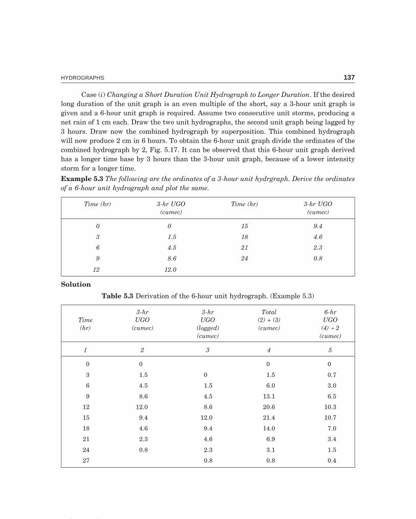
C-9\N-HYDRO\HYD5-1.PM5 137
HYDROGRAPHS 137
Case (i) Changing a Short Duration Unit Hydrograph to Longer Duration. If the desiredlong duration of the unit graph is an even multiple of the short, say a 3-hour unit graph isgiven and a 6-hour unit graph is required. Assume two consecutive unit storms, producing anet rain of 1 cm each. Draw the two unit hydrographs, the second unit graph being lagged by3 hours. Draw now the combined hydrograph by superposition. This combined hydrographwill now produce 2 cm in 6 hours. To obtain the 6-hour unit graph divide the ordinates of thecombined hydrograph by 2, Fig. 5.17. It can be observed that this 6-hour unit graph derivedhas a longer time base by 3 hours than the 3-hour unit graph, because of a lower intensitystorm for a longer time.
Example 5.3 The following are the ordinates of a 3-hour unit hydrgraph. Derive the ordinatesof a 6-hour unit hydrograph and plot the same.
Time (hr) 3-hr UGO Time (hr) 3-hr UGO(cumec) (cumec)
0 0 15 9.4
3 1.5 18 4.6
6 4.5 21 2.3
9 8.6 24 0.8
12 12.0
Solution
Table 5.3 Derivation of the 6-hour unit hydrograph. (Example 5.3)
3-hr 3-hr Total 6-hrTime UGO UGO (2) + (3) UGO(hr) (cumec) (logged) (cumec) (4) ÷ 2
(cumec) (cumec)
1 2 3 4 5
0 0 0 0
3 1.5 0 1.5 0.7
6 4.5 1.5 6.0 3.0
9 8.6 4.5 13.1 6.5
12 12.0 8.6 20.6 10.3
15 9.4 12.0 21.4 10.7
18 4.6 9.4 14.0 7.0
21 2.3 4.6 6.9 3.4
24 0.8 2.3 3.1 1.5
27 0.8 0.8 0.4
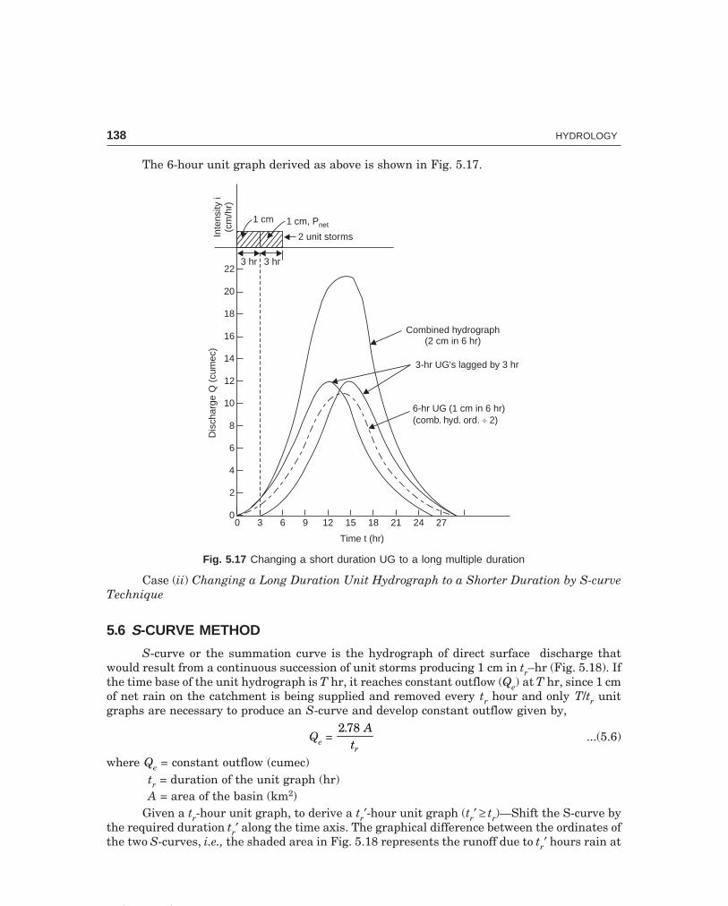
C-9\N-HYDRO\HYD5-2.PM5 138
138 HYDROLOGY
The 6-hour unit graph derived as above is shown in Fig. 5.17.
2724211815129630
22
20
18
16
14
12
10
8
6
4
2
0
Inte
nsity
i(c
m/h
r)1 cm 1 cm, Pnet
2 unit storms
3 hr3 hr
Combined hydrograph(2 cm in 6 hr)
3-hr UG's lagged by 3 hr
6-hr UG (1 cm in 6 hr)(comb. hyd. ord. 2)¸
Dis
char
geQ
(cum
ec)
Time t (hr)
Fig. 5.17 Changing a short duration UG to a long multiple duration
Case (ii) Changing a Long Duration Unit Hydrograph to a Shorter Duration by S-curveTechnique
5.6 S-CURVE METHOD
S-curve or the summation curve is the hydrograph of direct surface discharge thatwould result from a continuous succession of unit storms producing 1 cm in tr–hr (Fig. 5.18). Ifthe time base of the unit hydrograph is T hr, it reaches constant outflow (Qe) at T hr, since 1 cmof net rain on the catchment is being supplied and removed every tr hour and only T/tr unitgraphs are necessary to produce an S-curve and develop constant outflow given by,
Qe = 2 78. A
tr...(5.6)
where Qe = constant outflow (cumec)tr = duration of the unit graph (hr)A = area of the basin (km2)
Given a tr-hour unit graph, to derive a tr′-hour unit graph (tr′ ≥ tr)—Shift the S-curve bythe required duration tr′ along the time axis. The graphical difference between the ordinates ofthe two S-curves, i.e., the shaded area in Fig. 5.18 represents the runoff due to tr′ hours rain at
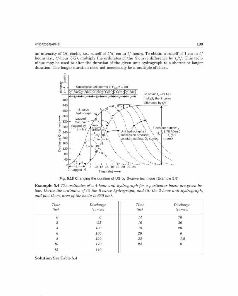
C-9\N-HYDRO\HYD5-2.PM5 139
HYDROGRAPHS 139
an intensity of 1/tr cm/hr, i.e., runoff of tr′/tr cm in tr′ hours. To obtain a runoff of 1 cm in tr′hours (i.e., tr′-hour UG), multiply the ordinates of the S-curve difference by tr/tr′. This tech-nique may be used to alter the duration of the given unit hydrograph to a shorter or longerduration. The longer duration need not necessarily be a multiple of short.
24222018161412108
480
440
400
360
320
280
240
200
160
120
80
40
0
Successive unit storms of P = 1 cmnet
1 cm1 cm 1 cm1 cm 1 cm1 cm 1 cm1 cm 1 cm1 cm 1 cm1 cm
trtr trtr trtr trtr trtr trtr
Inte
nsity
=(c
m/h
r)i
1 t r
S-curvehydrograph
LaggedS-curve
(lagged byt – hr)r
To obtain t – hr UGmultiply the S-curvedifference by t /t
r
r r¢
Constant outflowConstant outflow
Q =eQ =e2.78 A(km )
t (hr)
2
rCumec
Unit hydrographs insuccession produceconstant outflow, Q cumece
Unit hydrographs insuccession produceconstant outflow, Q cumece
´́ tr
r
��
cm
in t – hr
tr� cm
in t – hrr�B
A
t – hr UGrt – hr UGr
Dis
char
geQ
(cum
ec)
Time t (hr)0 6
tr�tr�Lagged
Areas-curvedifference
=
Areas-curvedifference
= 1tr1tr
2 4
Fig. 5.18 Changing the duration of UG by S-curve technique (Example 5.5)
Example 5.4 The ordinates of a 4-hour unit hydrograph for a particular basin are given be-low. Derive the ordinates of (i) the S-curve hydrograph, and (ii) the 2-hour unit hydrograph,and plot them, area of the basin is 630 km2.
Time Discharge Time Discharge(hr) (cumec) (hr) (cumec)
0 0 14 70
2 25 16 30
4 100 18 20
6 160 20 6
8 190 22 1.5
10 170 24 0
12 110
Solution See Table 5.4

C-9\N-HYDRO\HYD5-2.PM5 140
140 HYDROLOGY
Tab
le 5
.4 D
eriv
atio
n o
f th
e S
-cu
rve
and
2-h
our
un
it h
ydro
grap
hs.
(E
xam
ple
5.4)
*Sli
ght
adju
stm
ent
is r
equ
ired
to
the
tail
of
the
2-h
our
un
it h
ydro
grap
h.
Col
(5)
: lag
ged
S-c
urv
e is
th
e sa
me
as c
ol (
4) b
ut
lagg
ed b
y t r′
= 2
hr.
Col
(7)
: col
(6)
×
t tr r′, t
r = 4
hr.
tr′
= 2
hr.
Col
(3)
: No.
of
un
it s
torm
s in
su
cces
sion
= T
/tr
= 24
/4 =
6, t
o pr
odu
ce a
con
stan
t ou
tflo
w.
Qe
= 2
78.
�
At r
=
278
630
4.
× =
437
cu
mec
, w
hic
h a
gree
s ve
ry w
ell
wit
h t
he
tabu
late
d S
-cur
ve t
erm
inal
val
ue o
f 43
6. T
he S
-cu
rve
addi
tion
s ca
n b
e w
ritt
en i
n o
ne
colu
mn
, wit
hou
t h
avin
g to
wri
te i
n 5
col
um
ns
succ
essi
vely
lag
ged
by 4
hou
rs (
= t r)
, as
is i
llu
stra
ted
in t
he
exam
ple
5.5.
Plo
t co
l (4
) ve
rsu
s co
l (1
) to
get
th
e S
-cu
rve
hyd
rogr
aph
, an
d co
l (7
) ve
rsu
s co
l (1
) to
get
th
e 2-
hou
r u
nit
hyd
rogr
aph
, as
sh
own
in
Fig
.5.1
9.
Tim
e4-
hr
UG
OS
-cu
rve
add
itio
ns
S-c
urv
ela
gged
S-c
urv
e2-
hr
UG
O(h
r)(c
um
ec)
(cu
mec
)or
din
ates
S-c
urv
ed
iffe
ren
ce(6
) ×
4/3
(un
it s
torm
s af
ter
ever
y 4
hr
= t
r)(c
um
ec)
(cu
mec
)(c
um
ec)
(cu
mec
)(2
) +
(3)
(4)
– (5
)
12
34
56
7
00
——
——
—0
—0
0
225
——
——
—25
025
50
410
00
——
——
100
2575
150
616
025
——
——
185
100
8517
0
819
010
00
——
—29
018
510
521
0
1017
016
025
——
—33
529
065
130
1211
019
010
00
——
400
355
4590
1470
170
160
25—
—42
540
025
50
1630
110
190
100
0—
430
425
510
*
1820
7017
016
025
—44
543
015
30
206
3011
019
010
00
436
445
– 9
– 18
*
221.
520
7017
016
025
446.
543
610
.521
240
630
110
190
100
436
446.
6–
10.5
– 21
*

C-9\N-HYDRO\HYD5-2.PM5 141
HYDROGRAPHS 141
Example 5.5 The ordinates of a 4-hour unit hydrograph for a particular basin are given be-low. Determine the ordinates of the S-curve hydrograph and therefrom the ordinates of the 6-hour unit hydrograph.
Time 4-hr UGO Time 4-hr UGO(hr) (cumec) (hr) (cumec)
0 0 12 110
2 25 14 70
4 100 16 30
6 160 18 20
8 190 20 6
10 170 22 1.5
24 0
Solution See Table 5.5.
Table 5.5 Derivation of the 6–hour UG for the basin (Example 5.5)
Time 4-hour S-curve1 S-curve lagged2 S-curve 6-hr(hr) UGO additions ordinates C-curve difference UGO
(cumec) (cumec) (cumec) (cumec) (cumec) (cumec)(2) + (3) (4) – (5) (6) × 4/6
1 2 3 4 5 6 7
0 0 → — 0 — 0 0
2 25 → — 25 — 25 16.7
4 100 + → 0 100 — 100 66.7
6 160 + → 25 185 0 185 123.3
8 190 100 290 25 265 176.7
10 170 185 355 100 255 170.0
12 110 290 400 185 215 143.3
14 70 355 425 290 135 90.0
16 30 400 430 355 75 50.0
18 20 425 445 400 45 30.0
20 6 430 436 425 11 7.3
22 1.5 445 446.6 430 16.5 11.0
24 0 436 436 445 – 9 – 6.0
1—Start the operation shown with 0 cumec after tr = 4 hr.
2—Lag the S–curve ordinates by tr′ = 6 hr.
Plot col (4) vs. col (1) to get S-curve hydrograph and col (7) vs. col (1) to get 6-hr unit hydrographas shown in Fig. 5.19.

C-9\N-HYDRO\HYD5-2.PM5 142
142 HYDROLOGY
5.7 BERNARD’S DISTRIBUTION GRAPH
The distribution graph, introduced by Bernard in 1935, shows the percentages of total unithydrograph, which occur during successive, arbitrarily chosen, uniform time increments,Fig. 5.20. It is an important concept of the unit hydrograph theory that all unit storms, regard-less of their intensity, produce nearly identical distribution graphs.
The procedure of deriving the distribution graph is first to separate the base flow fromthe total runoff; the surface runoff obtained is divided into convenient time units, and theaverage rate of surface runoff during each interval is determined.
If the rainfall-runoff data for a short duration fairly uniform storm is known, the dura-tion of net rainfall is taken as the unit period and the distribution percentages are computeddirectly. But if there are multiple storms of different intensities producing different net rainsduring successive unit periods, a trial and error procedure of applying the distribution per-centages is followed, till the direct surface runoff during successive time intervals correspondsto the computed values. Once a distribution graph is derived for a drainage basin, any ex-pected volume of surface runoff from the basin can be converted into a discharge hydrograph.By drawing a smooth curve along the steps of the distribution graph to give equal areas, a unithydrograph may be obtained as shown in Fig. 5.20.Example 5.6 Analysis of the runoff records for a one day unit storm over a basin yields thefollowing data:
480
440
400
360
320
280
240
200
160
120
80
40
026242220181614121086420
S-curve hydrograph
S-curve lagged by t = 2 hrr¢
S-curve differencearea
6-hr (Derived)-Example 5.5UG2-hr (Derived)-Example 5.4UG
4-hr UG (given)
A – B = 65 m /s3 A
B
itr
= t´ r¢ cm in – hrtr¢Q =e
To get 1 cm in t , i.e., t -hr UG:r r¢ ¢Multiply the S-curve difference by
ttr
r
¢ t
tr
r¢´i.e., = 1 cm in t -hrr¢
(A – B)t
tr
r¢
42
= 2 hr lag
trtr¢ Time t (hr)
Dis
char
geQ
(cum
ec)
2.78 (630)4
2.78 (630)4
= 437 cumec= 437 cumec
= 65
= 130 cumec
´
t
tr
r¢
Fig. 5.19 Derivation of 2-hr & 6-hr UG from a 4-hr UG (Example 5.4 & 5.5)
Total stream flow at concentration point on successive days are 19.6, 62.4, 151.3, 133.0,89.5, 63.1, 43.5, 28.6, and 19.6 cumec.
Estimated base flow during the corresponding period on successive days are 19.6, 22.4,25.3, 28.0, 28.0, 27.5, 25.6, 22.5 and 19.6 cumec.

C-9\N-HYDRO\HYD5-2.PM5 143
HYDROGRAPHS 143
Determine the distribution graph percentages.On the same basin (area = 2850 km2) there was rainfall of 7 cm/day on July 15 and 10
cm/day on July 18 of a certain year. Assuming an average storm loss of 2 cm/day, estimate thevalue of peak surface runoff in cumec and the date of its occurrence.
Table 5.6 Derivation of distribution percentages
Day since DRO on Percentagebeginning of mid-day of Remarksdirect runoff (cumec) ΣDRO
1 2 3 4
1 18 4.5 = 18
402100×
2 96 243 120 304 82 205 47 126 25 67 12 38 2 0.5
8 equal time Σ DRO = 402 Total = 100.0(i.e., a day) intervals
1 2 3 4 5 6 7 8 9 10
Time base T divided into 10 unit periods
Unit periods
+ve & –ve areas should balance(area under bar graph = area under UG)
t – hr r UG
Distribution percentagessame for all unit storms
Distribution graph
Distribution % × 100=0i
0S i
Unit period25%
19.5%
16 %
+ 12%
9%
5.5%
3%
1%0909
0808
0707
0606
0505
0404
0303
0202
01
7%
2%
%of
tota
ldis
char
ge
trtr
P = x cmnet
P =1cmnetInte
nsity
i(cm
/hr)
010010
–
Fig. 5.20 Distribution graph (after Bernard, 1935)

C-9\N-HYDRO\HYD5-2.PM5 144
144 HYDROLOGY
Solution The total runoff hydrograph and estimated base flow are drawn in Fig. 5.21 and thedirect runoff ordiantes on successive mid-days are determined as DRO = TRO – BFO and thepercentages of direct runoff on successive days computed in Table 5.6. Column (3) gives the distri-bution percentages, and the derived distribution graph for 1-day unit storms is shown in Fig. 5.22.
150
140
130
120
110
100
90
80
70
60
50
40
30
20
10
01 2 3 4 5 6 7 8 9 10 110
Time t (days)
Base flow
Direct surfacerunoff
Direct surfacerunoff
4747
2525
12122
8282
120120
9696
1818
Streamflow hydrograph
Mid-ordinates (cumec)
Dis
char
geQ
(cum
ec)
160
Fig. 5.21 Stream flow hydrograph (Example 5.6)
36
32
28
24
20
16
12
8
4
0 1 2 3 4 5 6 7 8
Distributionpercentages
30
20
24
12
6
30.5
4.5
%of
tota
lsur
face
runo
ff
1-day unit periods
Fig. 5.22 Derived distribution graph (Example 5.6)

C-9\N-HYDRO\HYD5-2.PM5 145
HYDROGRAPHS 145
1210 11876543210 9
1000
800
600
400
200
0
Runoff hydrographdue to 2-storms onJuly 15 & 18
892 cumec (peak flood)
Dire
ctsu
rfac
eru
noff
(cum
ec)
July 15 16 17 18 19 20 21 22 23 24 25 26
Days (date)
Fig. 5.23 Runoff Hydrograph (Example 5.6)
Applying the distribution percentages computed in col. (3) above the direct surface dis-charge on successive days due to the two storms (lagged by 3 days) is computed in Table 5.7
1 cm/day = 1
1002850 1024 60 60
6
× ×× ×
= 330 cumec
The peak surface runoff is 892 cumec and occurs on July 20 of the year. The floodhydrograph is shown in Fig. 5.23.Example 5.7 Analysis of rainfall and runoff records for a certain storm over a basin (of area3210 km2) gave the following data:
Rainfall for successive 2 hr periods: 2.5, 6.5 and 4.5 cm/hr.An average loss of 1.5 cm/hr can be assumed.Direct surface discharge at the concentration point for successive 2-hr periods: 446, 4015,
1382, 25000, 20520, 10260, 4900 and 1338 cumec.Derive the unit hydrograph in the form of distribution percentages on the basis 2-hr unit
periods.Solution The rainfall may be considered for three unit periods of 2 hr each, then from Fig. 5.24,
TDSR = tR + Tr ...(5.7)T = tr + Tr ...(5.7 a)
∴ T = tr + TDSR – tR
= 2 + 8 × 2 – 3 × 2 ...(5.7 b)∴ T = 12 hr

C-9\N-HYDRO\HYD5-2.PM5 146
146 HYDROLOGY
Un
it p
erio
ds
(day
)
12
34
56
78
910
11
Tot
al r
ain
fall
(cm
)→
710
Los
s of
rai
n (
cm)
→2
2
Net
rai
n (
cm)
→5
8 (
= 13
cm
)
Un
it d
istr
ibu
tion
Dis
trib
uti
on (
cm/d
ay)
Per
iods
Per
cen
tage
s
14.
50.
225
0.36
224
1.20
1.92
330
1.50
2.40
420
1.00
1.60
512
0.60
0.96
66
0.30
0.48
73
0.15
0.24
80.
50.
025
0.04
Tot
al (
cm/d
ay):
0.22
51.
201.
501.
362.
522.
701.
750.
985
0.48
0.24
0.04
= 1
3 cm
(ch
eck)
× 33
0 =
cum
ec:
7439
649
545
083
389
257
832
515
879
13 (
0.22
5 ×
330)
= 74
cu
mec
)
Dat
e: J
uly
1516
1718
1920
2122
2324
25
Tab
le 5
.7 A
ppli
cati
on o
f di
stri
buti
on p
erce
nta
ges
to c
ompu
te t
he
dire
ct s
urf
ace
disc
har
ge (
Exa
mpl
e 5.
6)

C-9\N-HYDRO\HYD5-2.PM5 147
HYDROGRAPHS 147
The base width is 12 hr or 6 unit periods. As a first trial, try a set of six distributionpercentages of 10, 20, 40, 15, 10, 5 which total 100%. The direct surface discharge can beconverted into cm/hr as
1 cm/hr = 1
1003210 10
60 60
6
× ××
= 8920 cumec
1 cm/hr
5 cm/hr3 cm/hr
Loss rate 1.5 cm/hr
Pnet
Inte
nsity
i(cm
/hr)
tRtR TrTrtrtr trtr trtr
Dis
char
geQ
(cum
ec)
TTTT
TTTDSRTDSR
Time t (hr)
3
21 Base time, T = t + T= t + T – t
r r
r DSR R
Combined hydrograph dueto 3-unit stroms 1,2 & 3
Hydrograph due to 3-unit storms
Duration of direct surfacerunoff, T = t + TDSR R r
t = unit durationt = rainfall durationT = recession time
r
R
r
Fig. 5.24 Combined hydrograph (Example 5.7)
Gauged
Computed (1 trial)st
T = 8 × 2= 16 hr
DSRT = 8 × 2= 16 hr
DSR
3.5
3.0
2.5
2.0
1.5
1.0
0.5
00 1 2 3 4 5 6 7 8
2-hr-unit periods
Dire
ctsu
rfac
eru
noff
(cm
/hr)
Dis
trib
utio
n%
(1tr
ial,
2tr
ial)
stnd
10, 510, 51
2 20, 2020, 203 40, 4040, 40
4 15, 2015, 205 10, 1010, 10
6 5, 55, 5
Fig. 5.25 Derivation of distribution percentages (Example 5.7)

C-9\N-HYDRO\HYD5-2.PM5 148
148 HYDROLOGY
2-h
r-u
nit
per
iod
s
12
34
56
78
Rai
nfal
l ra
te (
cm/h
r) →
2.5
6.5
4.5
Los
s ra
te (
cm/h
r) →
1.5
1.5
1.5
Net
rai
n (
cm/h
r) →
15
3 (
= 9
× 2
cm)
Un
it d
istr
ibu
tion
Dis
trib
uti
on (
cm/h
r)
Per
iods
Per
cen
tage
1
10
(5)
(0.0
5)(0
.25)
(0.1
5)
0.10
0.50
0.30
22
00.
201.
000.
60
34
00.
402.
001.
20
415
(20
)(0
.20)
(1.0
0)(0
.60)
0.15
0.75
0.45
51
00.
100.
500.
30
65
0.05
0.25
0.15
Tot
al 1
00 (
100)
cm
/hr
0.10
0.70
1.70
2.75
2.05
1.00
0.55
0.15
(= 9
× 2
cm
ch
eck)
(0.0
5)(0
.45)
(1.5
5)(2
.80)
(2.3
0)(1
.15)
c um
ec44
640
1513
8225
000
2052
010
260
4900
1338
(446
/892
0 =
0.05
cm
/hr)
Not
e F
igu
res
in b
rack
ets
indi
cate
th
e ad
just
ed v
alu
es i
n t
he
seco
nd
tria
l.
Tab
le 5
.8 D
eriv
atio
n o
f di
stri
buti
on p
erce
nta
ges
by t
rial
s (E
xam
ple
5.7)

C-9\N-HYDRO\HYD5-2.PM5 149
HYDROGRAPHS 149
and the direct surface runoff for successive 2-hr periods are 0.05, 0.45, 1.55, 2.80, 2.30, 1.15,0.55, and 0.15 cm/hr. The first trial hydrograph computed in Table 5.8 is shown by dashedlines in Fig. 5.25 for comparison and selection of the distribution percentages for the secondtrial. The first percentage affects the first 3 unit periods, the second percentage affects the2nd, 3rd and 4th unit periods and like that. Since the first trial hydrograph gives higher val-ues (than gauged) for the first three unit periods, a lower percentage of 5 (instead of 10%) istried. Similarly, the other percentages are adjusted till the computed discharge values agreewith the gauged values. Thus, the second trial distribution percentages are 5, 20, 40, 20, 10, 5which total 100 and are final and the distribution graph thus derived is shown in Fig. 5.26. Inmost cases, more trials are required to obtain the desired degree of accuracy.
Also see Appendix—G.
20 20
1055
40
60
50
40
30
20
10
0
%of
tota
ldire
ctsu
rfac
eru
noff
00 1 2 3 4 5 62-hr unit periods
Fig. 5.26 Derived distribution graph (Example 5.7)
5.8 INSTANTANEOUS UNIT HYDROGRAPH
The difficulty of using a unit hydrograph of a known duration has been obviated by the devel-opment of the instantaneous unit hydrograph (IUH). The IUH is a hydrograph of runoff re-sulting from the instantaneous application of 1 cm net rain on the drainage basin. The IUH inconjunction with the design storm can be used to obtain the design flood by using a convolutionintegral. The IUH was first proposed by Clark in 1945. The IUH can be developed eitherdirectly from the observed data or by adopting conceptual models [see Chapter–16 & 17 forMethods of Determining IUH].
5.9 SYNTHETIC UNIT HYDROGRAPHS
In India, only a small number of streams are gauged (i.e., streamflows due to single and mul-tiple storms, are measured). There are many drainage basins (catchments) for which nostreamflow records are available and unit hydrographs may be required for such basins. Insuch cases, hydrographs may be synthesised directly from other catchments, which arehydrologically and meteorologically homogeneous, or indirectly from other catchments throughthe application of empirical relationship. Methods for synthesising hydrographs for ungaugedareas have been developed from time to time by Bernard, Clark, McCarthy and Snyder. Thebest known approach is due to Snyder (1938). Snyder analysed a large number of hydrographsfrom drainage basins in the Applachian Mountain region in USA ranging in the area from 25to 25000 km2 and selected the three parameters for the development of unit hydrograph, namely,

C-9\N-HYDRO\HYD5-2.PM5 150
150 HYDROLOGY
base width (T), peak discharge (Qp) and lag time (basin lag, tp), Fig. 5.27, and proposed thefollowing empirical formulae for the three parameters:
Lag time, tp = Ct (L Lca)0.3 ...(5.8)
standard duration of net rain, tr = tp
5 5....(5.9)
1/31/3 2/32/3W50W50
Area undercurve = 1 cmrunoff volume
0.5Q
p0.
5Qp
0.75
Qp
0.75
Qp
W75W75
1/3 2/32/3
Syntheticunit hydrograph
W = hr505.6qp
1.08
W = hr753.21
qp1.08
q = cumec/kmp2Q
Ap
t = , Snyderr
t
5.5p
t = C (L.L )p t ca0.3
Q = Cp pAtp
T 5 t hr» p
Peak flow
Basin lagtptptr
2
tr2
QpQp
Dis
char
geQ
(cum
ec)
Base time T (days or hr)
Time t (hr)
Inte
nsity
i=(c
m/h
r)1 t r
Unit duration
P = 1 cmnetCentre of Pnet
tr
Fig. 5.27 Synthetic unit hydrograph parameters
For this standard duration of net rain,
peak flow, Qp = Cp Atp
...(5.10)
time base in days, T = 3 + 3 tp
24FHG
IKJ ...(5.11)
peak flow per km2 of basin, qp = Q
tp
p...(5.12)
Snyder proposed subsequently an expression to allow for some variation in the basin lagwith variation in the net rain duration, i.e., if the actual duration of the storm is not equal to trgiven by Eq. (5.9) but is tr′, then
tpr = tp + ′ −t tr r
4...(5.13)
where tpr = basin lag for a storm duration of tr′, and tpr is used instead of tp in Eqs. (5.10),(5.11) and (5.12).
In the above equations,tp = lag time (basin lag), hr

C-9\N-HYDRO\HYD5-2.PM5 151
HYDROGRAPHS 151
Ct, Cp = empirical constants (Ct ≈ 0.2 to 2.2, Cp ≈ 2 to 6.5, the values depending on thebasin characteristics and units)
A = area of the catchment (km2)L = length of the longest water course, i.e., of the mainstream from the gauging
station (outlet or measuring point) to its upstream boundary limit of the basin,(km) (Fig. 5.28)
Lca = length along the main stream from the gauging station (outlet) to a point on thestream opposite the areal centre of gravity (centroid) of the basin
L kmcaL kmcaL kmL kmCentroid ofbasin
Main water courseUpstreamboundaryof river
Point inriver opp.centroid
Tributary
Area ofbasin A, km
2
River
Basin boundary
Basin lag (Snyder)
t = c (L.L )p t ca0.3
Basin slope, S
GaugingStn.
(outlet)
Tributary
Taylor & SchwarzC = , a = Constantt
a
s
Linsley, et al.
t = c ( )p tnL.L
Sca
Fig. 5.28 Basin characteristics (Snyder)
Snyder considered that the shape of the unit hydrograph is likely to be affected by thebasin characteristics like area, topography, shape of the slope, drainage density and channelstorage. He dealt with the size and shape of basin by measuring the length of the mainstreamchannel. The coefficient Ct reflects the size, shape and slope of the basin.
Linsley, Kohler and Paulhus gave an expression for the lag time in terms of the basincharacteristics (see Fig. 5.31) as
tp = Ct LL
Sca
nFHG
IKJ ...(5.14)
where S = basin slope, and the values of n and Ct, when L, Lca were measured in miles are n = 0.38Ct = 1.2, for mountainous region = 0.72, for foot hill areas = 0.35, for valley areas
Taylor and Scwarz found from an analysis of 20 drainage basins of size 50-4000 km2 inthe north and middle Atlantic States in USA that (when L and Lca were measured in miles)
Ct = 0 6.
S...(5.15)
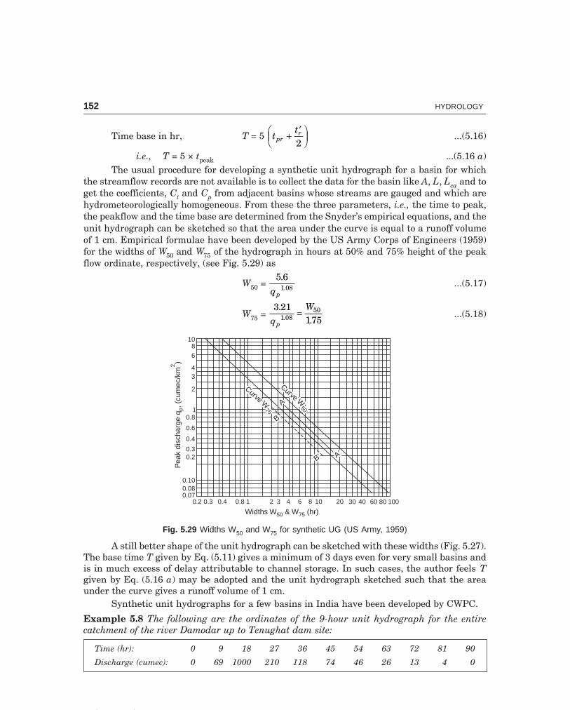
C-9\N-HYDRO\HYD5-2.PM5 152
152 HYDROLOGY
Time base in hr, T = 5 tt
prr+ ′F
HGIKJ2
...(5.16)
i.e., T = 5 × tpeak ...(5.16 a)The usual procedure for developing a synthetic unit hydrograph for a basin for which
the streamflow records are not available is to collect the data for the basin like A, L, Lca and toget the coefficients, Ct and Cp from adjacent basins whose streams are gauged and which arehydrometeorologically homogeneous. From these the three parameters, i.e., the time to peak,the peakflow and the time base are determined from the Snyder’s empirical equations, and theunit hydrograph can be sketched so that the area under the curve is equal to a runoff volumeof 1 cm. Empirical formulae have been developed by the US Army Corps of Engineers (1959)for the widths of W50 and W75 of the hydrograph in hours at 50% and 75% height of the peakflow ordinate, respectively, (see Fig. 5.29) as
W50 = 5 6
1 08
..qp
...(5.17)
W75 = 3 21
1751 0850.
..qW
p
= ...(5.18)
Curve W50
Curve W50
Curve W75
Curve W75
B�B�
BB
AA
108
6
43
2
10.8
0.6
0.4
0.30.2
0.100.080.07
0.2 0.3 0.4 0.8 1 2 3 4 6 8 10 20 30 40 60 80 100
Pea
kdi
scha
rge
q, (
cum
ec/k
mp
2 )
Widths W & W (hr)50 75
A�A�
Fig. 5.29 Widths W50 and W75 for synthetic UG (US Army, 1959)
A still better shape of the unit hydrograph can be sketched with these widths (Fig. 5.27).The base time T given by Eq. (5.11) gives a minimum of 3 days even for very small basins andis in much excess of delay attributable to channel storage. In such cases, the author feels Tgiven by Eq. (5.16 a) may be adopted and the unit hydrograph sketched such that the areaunder the curve gives a runoff volume of 1 cm.
Synthetic unit hydrographs for a few basins in India have been developed by CWPC.
Example 5.8 The following are the ordinates of the 9-hour unit hydrograph for the entirecatchment of the river Damodar up to Tenughat dam site:
Time (hr): 0 9 18 27 36 45 54 63 72 81 90
Discharge (cumec): 0 69 1000 210 118 74 46 26 13 4 0

C-9\N-HYDRO\HYD5-2.PM5 153
HYDROGRAPHS 153
and the catchment characteristics areA = 4480 km2, L = 318 km, Lca = 198 km
Derive a 3-hour unit hydrograph for the catchment area of river Damodar up to the headof Tenughat reservoir, given the catchment characteristics as:
A = 3780 km2, L = 284 km, Lca = 184 kmUse Snyder’s approach with necessary modifications for the shape of the hydrograph.
Solution The 9-hr UG is plotted in Fig. 5.30 and from that tp = 13.5 hr
tr = 9 hr,tp
5 513 55 5.
..
= = 2.46 hr ≠ tr of 9 hr
∴ tr′ = 9 hr, tpr = 13.5 hr and tp has to be determined
tpr = tp + ′ −t tr r
4
13.5 = tp + 9 5 5
4
− tp/ .
∴ tp = 11.8 hrtp = Ct (LLca)0.3
11.8 = Ct (318 × 198)0.3
∴ Ct = 0.43
Peak flow, Qp = Cp A
tpr
1000 = Cp 448013 5.
∴ Cp = 3.01, say, 3The constants of Ct = 0.43 and Cp = 3 can now be applied for the catchment area up to
the head of the Tenughat reservoir, which is meteorologically and hydrologically similar.tp = Ct (LLca)0.3 = 0.43 (284 × 184)0.3 = 11.24 hr
tp
5 511245 5...
= = 2.04 hr ≠ tr of 3 hr (duration of the required UG)
∴ tr′ = 3 hr, tr = 2.04 hr and tpr has to be determined.
tpr = tp + ′ −t tr r
4 = 11.24 +
3 2 044
− .
∴ tpr = 11.48 hr, say, 11.5 hr
Peak flow Qp = Cp A
tpr = 3 ×
3780115.
= 987 cumec
Time to peak from the beginning of rising limb
tpeak = tpr + ′tr
2 = 11.5 +
32
= 13 hr
Time base (Snyder’s) T (days) = 3 + 3 tpr
24FHG
IKJ = 3 + 3
11.524
FHG
IKJ = 4.44 days or 106.5 hr

C-9\N-HYDRO\HYD5-2.PM5 154
154 HYDROLOGY
This is too long a runoff duration and hence to be modified as T(hr) = 5 × tpeak = 5 × 13 = 65 hr
To obtain the widths of the 3-hr UG at 50% and 75% of the peak ordinate :
qp = Q
Ap =
9873780
= 0.261 cumec/km2
W50 = 5 6 5 6
0 26108 08
.( )
.( . )qp
1. 1.= = 23.8 hr
W75 = 3 21 3 21
0 26108 08.
( ).
( . )qp1. 1.= = 13.6 hr =
23 8175
..
These widths also seem to be too long and a 3-hr UG can now be sketched using theparameters Qp = 987 cumec, tpeak = 13 hr and T = 65 hr such that the area under the UG isequal to a runoff volume of 1 cm, as shown in Fig. 5.30.
Synthetic unit hydrograph (3-hr)(constants: C = 0.86, C = 3) for
basin upto head of reservoirt p
Area underUG = 1 cm
runoff volume
9-hr UG for the entire basinupto Tenughat dam site
0 9 18 27 36 45 54 63 72 81 90
Inte
nsity
i=(c
m/h
r)1 t r
9 hr9 hr
P = 1 cmnet
13.513.54.5hr
Pnet3 hr3 hr1.5
hr 11.5hr
11.5hr
987cumecpeakflow
W75
1000 cumec peakflow
W50
1000
900
800
700
1000
600
500
400
300
200
100
0
Dis
char
geQ
(cum
ec)
Base time T = 65 hr
Time t (hr)
Base time T = 65 hr
Time t (hr)
Fig. 5.30 Synthetic unit hydrograph derived (Example 5.8)
5.10 TRANSPOSING UNIT HYDROGRAPHS
From Eq. (5.14)
tp = Ct LL
Sca
nFHG
IKJ

C-9\N-HYDRO\HYD5-2.PM5 155
HYDROGRAPHS 155
log log logt C np t��� ���= +
B LL
Sca
���
y = c + m x
Hence, a plot of tp vs. LL
Sca on log-log paper from data from basins of similar hydrologic
characteristics gives a straight-line relationship (Fig. 5.31). The constant Ct = tp when LL
Sca
= 1, and the slope of the straight line gives n. It may be observed that for basins having differ-ent hydrologic characteristics the straight lines obtained are nearly parallel, i.e., the values ofCt varies depending upon the slope of the basin (as can be seen from Eq. 5.15) but the value ofn is almost same.
Log-log paper
Determinationof C & n fromdata of gauged basins
t
for mountainous region
for foot hill areas
for valleys
1
2
3
t = c ( )p tnLL
Sca
n =Slopenn
LL
Sca
= 1
C = t , whent p
Slope n
Slope n
1
2
3
1008060
4030
20
1086543
2
12 3 4 6 8 10 20 100 100030 40 60 200 400
1000
1
10
100100101
km2
Bas
inla
gt
(hr)
p
LL
Sca
DyDx
Dy
Dx
Fig. 5.31 Basin lag vs. basin characteristics
From a plot of qp vs. tp, or from dimensionless hydrographs from gauged basins, thepeak flow and the shape of the unit hydrograph for ungauged basins can be estimated pro-vided they are hydrometeorologically the same. The dimensionless unit hydrographs elimi-nates the effect of basin size and much of the effect of basin shape. Hence, it is a useful meansfor comparison of unit hydrographs of basins of different sizes and shapes or those resultingfrom different storm patterns. It can be derived from a unit hydrograph by reducing its timeand discharge scales by dividing by tp and Qp, respectively. By averaging a number ofdimensionless unit hydrographs of drainage areas, a representative dimensionless graph canbe synthesized for a particular hydrological basin. A unit hydrograph for an ungauged basin,hydrologically similar, can be obtained directly from this dimensionless graph by multiplyingby the appropriate values of tp (obtained from log-log plot) and Qp (from a plot of qp vs. tp).

C-9\N-HYDRO\HYD5-3.PM5 156
156 HYDROLOGY
Example 5.9 For the 9-hr UG given for the entire catchment of the river Damodar in Example5.8, derive a dimensionless unit hydrograph.
Solution From example 5.8, tp = 11.8 hr, Qp = 1000 cumec, and hence the following computa-tion can be made:
ttp
: 0 0.763 1.525 2.29 3.05 3.82 4.58 5.34 6.10 6.87 7.63
QQp
: 0 0.069 1 0.21 0.118 0.074 0.046 0.026 0.013 0.004 0
The dimensionless unit hydrograph is plotted as shown in Fig. 5.32.
Dimensionlessunit hydrograph
(t/tp)0 1 2 3 4 5 6 7 8
1.0
0.9
0.8
0.7
0.6
0.5
0.4
0.3
0.2
0.1
0
(Q/Q
p)
Fig. 5.32 Dimensionless unit hydrograph
The US Soil Conservation Service (1971), using many hydrographs from drainage areasof varying sizes and different geographical locations, has developed a dimensionless unithydrograph and has developed the following formulae.
tpeak = t tc c+ 0 133
7.
1.and qp =
0 208. AQtpeak
where tc = time of concentration (hr)tpeak = time to peak discharge from beginning (hr)
= t
trp2
+ , where tp is lag time
qp = peak discharge (cumec) A = drainage area (km2) Q = quantity of runoff, which is 1 mm for the unit hydrograph

C-9\N-HYDRO\HYD5-3.PM5 157
HYDROGRAPHS 157
Most hydrologists assume tc as the time from the end of rainfall excess (Pnet) to the pointof inflection on the falling limb of the hydrograph; tpeak can be determined from tc or lag time tp.(basin lag) for the required tr-hr UG. From tpeak and known drainage area qp can be determined.Once tpeak and qp are obtained, ‘t vs. q’ can be computed from the data of the dimensionless unithydrograph and the UG can be sketched.Example 5.9 (a) Construct a 4-hr UH for a drainage basin of 200 km2 and lag time 10 hr bythe SCS method, given (pk = peak):
ttpk
: 0.5 1 2 3 4 5
QQp
: 0.4 1 0.32 0.075 0.018 0.004
Solution tpk = tr
2 + tp =
42
+ 10 = 12 hr
(i) Qp = 5 36 5 36 200
12. .Atpk
=×
= 89.33 cumec, which occurs at t
tpk = 1
or t = tpk = 12 hr
(ii) At t
tpk = 0.5 or t = 0.5 × 12 = 6 hr,
QQp
= 0.4 or Q = 0.4 × 89.33 = 35.732 cumec
(iii) At t
tpk = 2 or t = 2 × 12 = 24 hr,
QQp
= 0.32 or Q = 0.32 × 89.33 = 28.6 cumec
(iv) At t
tpk = 3 or t = 3 × 12 = 36 hr,
QQp
= 0.075, or Q = 0.075 × 89.33 = 6.7 cumec
Time base T = 5 tpk = 5 × 12 = 60 hr; W75 = W50/1.75
With this, a 4-hr UH can be sketched.
5.11 APPLICATION OF UNIT HYDROGRAPH
The application of unit hydrograph consists of two aspects:(i) From a unit hydrograph of a known duration to obtain a unit hydrograph of the
desired duration, either by the S-curve method or by the principle of superposition.(ii) From the unit hydrograph so derived, to obtain the flood hydrograph corresponding
to a single storm or multiple storms. For design purposes, a design storm is assumed, whichwith the help of unit hydrograph, gives a design flood hydrograph.
While the first aspect is already given, the second aspect is illustrated in the followingexample.
Example 5.10 The 3-hr unit hydrograph ordinates for a basin are given below. Therewas a storm, which commenced on July 15 at 16.00 hr and continued up to 22.00 hr, which wasfollowed by another storm on July 16 at 4.00 hr which lasted up to 7.00 hr. It was noted fromthe mass curves of self-recording raingauge that the amount of rainfall on July 15 was 5.75 cmfrom 16.00 to 19.00 hr and 3.75 cm from 19.00 to 22.00 hr, and on July 16, 4.45 cm from 4.00 to7.00 hr. Assuming an average loss of 0.25 cm/hr and 0.15 cm/hr for the two storms, respectively,

C-9\N-HYDRO\HYD5-3.PM5 158
158 HYDROLOGY
and a constant base flow of 10 cumec, determine the stream flow hydrograph and state the timeof occurrence of peak flood.
Time (hr): 0 3 6 9 12 15 18 21 24 27
UGO (cumec): 0 1.5 4.5 8.6 12.0 9.4 4.6 2.3 0.8 0
Solution Since the duration of the UG is 3 hr, the 6-hr storm (16.00 to 22.00 hr) can beconsidered as 2-unit storm producing a net rain of 5.75 – 0.25 × 3 = 5 cm in the first 3-hr periodand a net rain of 3.75 – 0.25 × 3 = 3 cm in the next 3-hr period. The unit hydrograph ordinatesare multiplied by the net rain of each period lagged by 3 hr. Similarly, another unit stormlagged by 12 hr (4.00 to 7.00 hr next day) produces a net rain of 4.45 – 0.15 × 3 = 4 cm which ismultiplied by the UGO and written in col (5) (lagged by 12 hr from the beginning), Table 5.9.The rainfall excesses due to the three storms are added up to get the total direct surfacedischarge ordinates. To this, the base flow ordinates (BFO = 10 cumec, constant) are added toget the total discharge ordinates (stream flow).
The flood hydrograph due to the 3 unit storms on the basin is obtained by plotting col (8)vs. col. (1) (Fig. 5.33). This example illustrates the utility of the unit hydrograph in derivingflood hydrographs due to a single storm or multiple storms occurring on the basin.
Date & Time t (hr)
Peak flood of 99 cumecon July 16, 07.00 hr
Streamflow hydrograph1 + 2 + 3 + B.F.
1
3
24 × UGO
Base flow = 10 cumec (constant)
16 19 22 01 4 7 10 13 16 19 22 01 4 7July 15July 15 July 16July 16 July 17July 17
Loss0.25 cm/hr
Loss0.15 cm/hr
3 cm 4 cm5 cm
3 hr 3 hr 3 hr
Pnet
6-hr storm split into2-unit periods
Inte
nsity
i(cm
/hr)
Dis
char
geQ
(cum
ec)
100
90
80
70
60
50
40
100
30
20
10
0
3 × UGO3 × UGO
5 × UGO5 × UGO
0 0
Fig. 5.33 Application of UG to obtain stream flow hydrograph (Example 5.10)

C-9\N-HYDRO\HYD5-3.PM5 159
HYDROGRAPHS 159D
RO
du
e to
rai
nfa
ll e
xces
sT
otal
Tim
eU
GO
*I
IIII
ID
RO
BF
OT
RO
Rem
arks
(hr)
UG
O ×
5 c
mU
GO
× 3
cm
UG
O ×
4 c
m(3
) +
(4)
+ (
5)(c
onst
ant)
(6)
+ (
7)
12
34
56
78
00
0—
—0
1010
.0–
July
15,
16.
00 h
r
31.
57.
50
—7.
510
17.5
com
men
cem
ent
of f
lood
64.
522
.54.
5—
27.0
1037
.0
98.
643
.013
.5—
56.5
1066
.5
1212
.060
.025
.80
85.8
1095
.8
159.
447
.036
.06
89.0
1099
.0—
Pea
k fl
ood
on J
uly
16,
184.
623
.028
.218
69.2
1079
.207
.00
hr
212.
311
.513
.834
.459
.710
69.7
240.
84.
06.
948
58.9
1068
.9
270
02.
437
.640
.010
50.0
300
18.4
18.4
1028
.4
339.
29.
210
19.2
363.
23.
210
13.2
390
010
10.0
— F
lood
su
bsid
es o
n Ju
ly 1
707
.00
hr
*All
col
um
ns
are
in c
um
ec u
nit
s ex
cept
col
(1)
.
Tab
le 5
.9 D
eriv
atio
n o
f th
e fl
ood
hyd
rogr
aph
du
e to
mu
ltip
le s
torm
s (E
xam
ple
5.10
)

C-9\N-HYDRO\HYD5-3.PM5 160
160 HYDROLOGY
Example 5.11 The design storm of a water shed has the depths of rainfall of 4.9 and 3.9 cm forthe consecutive 1-hr periods. The 1-hr UG can be approximated by a triangle of base 6 hr witha peak of 50 cumec occurring after 2 hr from the beginning. Compute the flood hydrographassuming an average loss rate of 9 mm/hr and constant base flow of 10 cumec. What is the areaof water shed and its coefficient of runoff?Solution (i) The flood hydrograph due to the two consecutive hourly storms is computed inTable 5.10, Fig. P5.34.
(ii) Area of water shed—To produce 1-cm net rain over the entire water shed (A km2). Volume of water over basin = Area of UG (triangle)
(A × 106) 1
100 = 1
2 (6 × 60 × 60) 50
from which, A = 54 km2
(iii) Coefficient of runoff C = RP
= − + −+
( . . ) ( . . ). .
4 9 0 9 3 9 0 94 9 3 9
= 0.795
Table 5.10 Computation of design flood hydrograph (Example 5.11)
Time UGO* DRO due to rain- Total BF TRO Remarks
(hr) (cumec) fall excess (cumec) (cumec) (cumec) (cumec)
4.9 – 0.9 3.9 – 0.9
= 4 cm = 3 cm
1 0 0 — 0 10 102 25 100 0 100 10 1103 50 200 75 275 10 2854 37.5 150 150 300 10 310 ← Peak flood†
5 25 100 112.5 212.5 10 222.56 12.5 50 75 125 10 1357 0 0 37.5 37.5 10 47.58 — — 0 0 10 10
*Ordinates by proportion in the triangular UG. †–Peak flood of 310 cumec, after 4 hr from thecommencement of the storm.
6543210
50
40
30
20
10
0
Peak
1-hr UG
Area 1 cm runoff�Q(c
umec
)
Time (hr)
2525
5050
37.5
37.5
2525
12.5
12.5
Fig. 5.34 (Example 5.11)
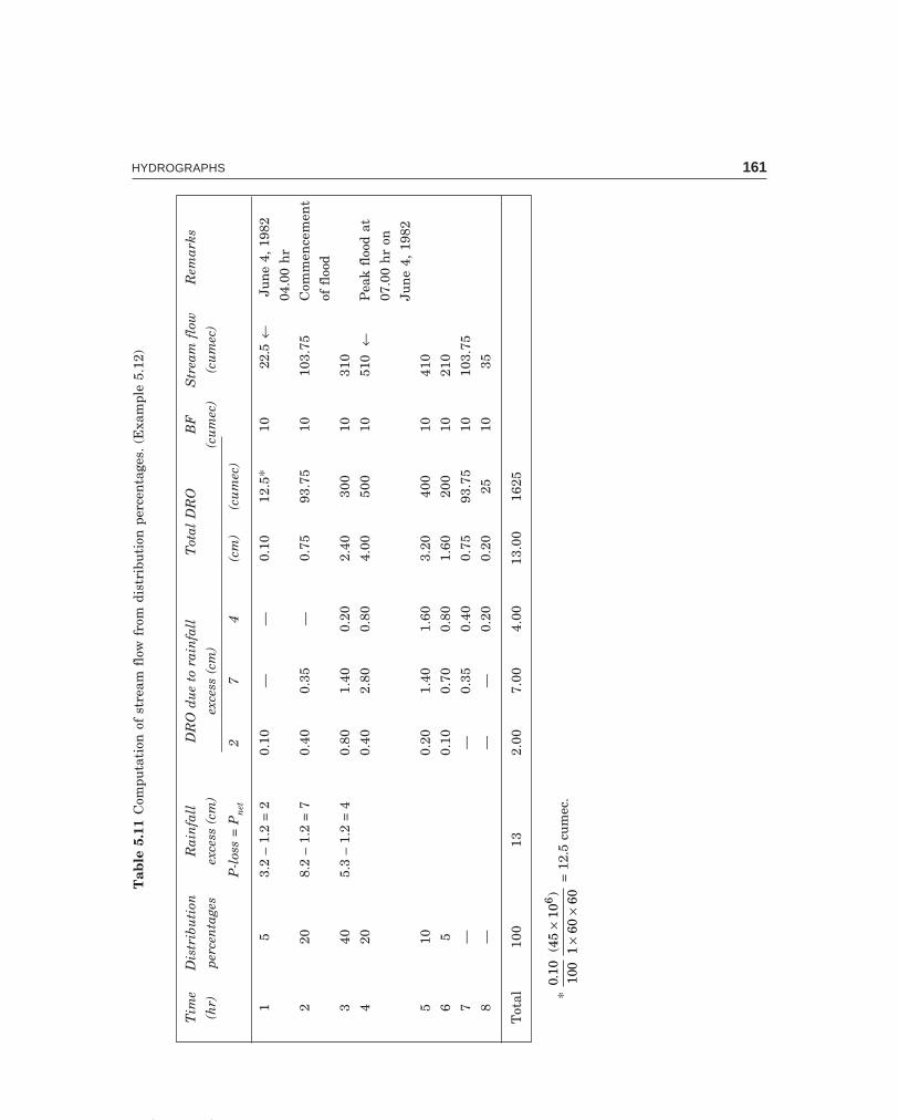
C-9\N-HYDRO\HYD5-3.PM5 161
HYDROGRAPHS 161
Tim
eD
istr
ibu
tion
Rai
nfa
llD
RO
du
e to
rai
nfa
llT
otal
DR
OB
FS
trea
m f
low
Rem
arks
(hr)
perc
enta
ges
exce
ss (
cm)
exce
ss (
cm)
(cu
mec
)(c
um
ec)
P-l
oss
= P
net
27
4(c
m)
(cu
mec
)
15
3.2
– 1.
2 =
20.
10—
—0.
1012
.5*
1022
.5 ←
Ju
ne
4, 1
982
04.0
0 hr
220
8.2
– 1.
2 =
70.
400.
35—
0.75
93.7
510
103.
75C
omm
ence
men
t
of f
lood
340
5.3
– 1.
2 =
40.
801.
400.
202.
4030
010
310
420
0.40
2.80
0.80
4.00
500
1051
0 ←
Pea
k fl
ood
at
07.0
0 h
r on
Jun
e 4,
198
2
510
0.20
1.40
1.60
3.20
400
1041
0
65
0.10
0.70
0.80
1.60
200
1021
0
7—
—0.
350.
400.
7593
.75
1010
3.75
8—
——
0.20
0.20
2510
35
Tot
al10
013
2.00
7.00
4.00
13.0
016
25
* 0
1010
045
101
60606
.(
)×
××
= 1
2.5
cum
ec.
Tab
le 5
.11
Com
puta
tion
of
stre
am f
low
fro
m d
istr
ibu
tion
per
cen
tage
s. (
Exa
mpl
e 5.
12)

C-9\N-HYDRO\HYD5-3.PM5 162
162 HYDROLOGY
Example 5.12 Storm rainfalls of 3.2, 8.2 and 5.2 cm occur during three successive hours overan area of 45 km2. The storm loss rate is 1.2 cm/hr. The distribution percentages of successivehours are 5, 20, 40, 20, 10 and 5. Determine the streamflows for successive hours assuming aconstant base flow of 10 cumec. State the peak flow and when it is expected; the precipitationstarted at 04.00 hr, on June 4, 1982.Solution The computation of stream flow hydrograph from the distribution percentages dueto net rainfall in three successive hours (i.e., from a complex storm) over an area of 45 km2 ismade in Table 5.11.Example 5.13 The successive three-hourly ordinates of a 6-hr UG for a particular basin are 0,15, 36, 30, 17.5, 8.5, 3, 0 cumec, respectively. The flood peak observed due to a 6-hr storm was150 cumec. Assuming a costant base flow of 6 cumec and an average storm loss of 6 mm/hr,determine the depth of storm rainfall and the streamflow at successive 3 hr interval.Solution DRO peak = Flood peak – BF
= 150 – 6 = 144 cumec
Pnet = DRO
UGpeak
peak =
14436
= 4 cm
Depth of storm rainfall, P = Pnet + losses = 4 + 0.6 × 6 = 7.6 cm. DRO = UGO × Pnet; DRO + BF = TRO
Hence, multiplying the given UGO by 4 cm and adding 6 cumec, the stream flow ordi-nates at successive 3-hr intervals are: 6, 66, 150, 126, 76, 40, 18, 6 cumec, respectively.
������
I Match the items in ‘A’ with items in ‘B’
A B
(i) Ground water depletion (a) Unit storm
(ii) Unit hydrograph (b) Flood hydrograph
(iii) TRO (c) Bernard
(iv) UGO (d) Synthetic unit hydrograph
(v) Unit duration (e) S-curve hydrograph
(vi) Change of unit duration (f) (TRO – BFO) ÷ Pnet
(vii) Distribution percentages (g) UGO × Pnet + BFO
(viii) Design storm (h) 1 cm of runoff
(ix) Ungauged stream (i) Base flow recession curve
II Say ‘true’ or ‘false’, if false, give the correct statement.
(i) Unit hydrographs should be used for basins, larger than 5000 km2.
(ii) Larger unit periods are required for larger basins.
(iii) If the peak of the unit hydrograph is 25 cumec, then the peak of the hydrograph producing 8cm of runoff is 215 cumec, assuming a constant base flow of 15 cumec.

C-9\N-HYDRO\HYD5-3.PM5 163
HYDROGRAPHS 163
(iv) The base flow of surface streams is the effluent seepage from the drainage basin.
(v) The ground water depletion curves are not of the same pattern for all the storms in a drain-age basin.
(vi) When dealing with small streams, a hydrograph of instantaneous flow should be constructed,wherever possible.
(vii) The best unit duration is about one-fourth of the basin lag.
(viii) The period of surface runoff is different for unit storms of different intensity.
(ix) If the period of surface runoff is divided into equal time intervals, the percentage of surfacerunoff that occurs during each of these intervals will be different for unit storms of differentintensities.
(x) The hydrograph of runoff for a basin reflects the combined physical characteristics of thebasin including infiltration, surface detention and storage.
(xi) The inflection point signifies gradual withdrawal of catchment storage.
(xii) The unit storm is of such duration that the period of surface runoff is much less for any otherstorm of shorter duration.
(xiii) The shape of the hydrograph of runoff will be affected by:
(i) the duration of the storm
(ii) areal distribution of the storm
(iii) the intensity of the storm (false: i, v, viii, ix, xii)
III Fill up the blanks correctly:
(i) The 3-hour unit hydrograph gives a net rain of ..... cm on the entire basin, for the rainfallduration of .... hours.
(ii) To convert a unit hydrograph of a known duration to some other required duration ... tech-nique is adopted.
(iii) The three basic propositions of the unit hydrograph theory are:
(a) .................
(b) .................
(c) .................
(iv) ............ hydrograph is constructed to serve as a unit hydrograph for a basin whose stream isnot gauged.
(v) The ground water contribution to the discharge in a stream is called .....
(vi) If the seepage from the stream builds up a ground water mound, such a stream is called.........
IV Choose the correct statement/s in the following:
1 A 4-hr unit (1 cm) hydrograph means
(i) the duration of rainfall is 4 hours.
(ii) the intensity of rainfall over the entire catchment is 2.5 mm/hr constant.
(iii) 1 cm depth of rainfall over the entire catchment.
(iv) 1 cm depth of rainfall excess over the entire catchment.
(v) a hydrograph resulting from the instantaneous application of 1 cm rainfall excess over thebasin.

C-9\N-HYDRO\HYD5-3.PM5 164
164 HYDROLOGY
(vi) that the stream flow is for 4 hours.
(vii) that the volume of direct surface runoff in the stream is 104 A m3 (A = area of basin in km2).
(viii) all the above.
2 Given a 4-hr unit (1 cm) hydrograph (UG), for any storm of 4-hr duration producing x cm ofrainfall excess
(i) the peak of direct runoff hydrograph (DRH) is x times the peak of UG.
(ii) the duration of direct surface runoff (DSR) is the same as that of UG.
(iii) if the duration of DSR in DRH and UG are divided into 8 unit periods, the percentage of DSRin the corresponding unit periods in both, is the same.
(iv) the ratio of the corresponding ordinates in each unit period of DRH and UG is x.
(v) all the above relations.
3 A S-curve hydrograph derived from a 4-hr UG (time base T = 24 hr) for a 640 km2 basin
(i) is the result of six 4-hr unit storms occurring in succession over the basin.
(ii) produces a constant outflow 445 cumec after 24 hours.
(iii) the constant outflow of 445 cumec is produced after 6 hours.
(iv) the shape of the curve in the first 24 hours is in the form of letter S.
(v) all the above items.
4 A synthetic unit hydrograph is developed
(i) for a basin whose stream is gauged.
(ii) for a basin over which no raingauge and stream gauge stations are established.
(iii) by measuring the mainstream lengths like L and Lca, and area of the basin.
(iv) by computing the basin slope.
(v) by taking certain constants from another basin, which is hydrometeorologically homogeneous.
(vi) for a basin having a raingauge network but with no stream gauging station
(viii) from items (iii) (v) and (vi) above.
5 The shape of the hydrograph is effected by
(i) non-uniform areal distribution of rainfall.
(ii) varying rainfall intensity.
(iii) shape of the basin.
(iv) direction of storm movement.
(v) all the above factors.
6 Given a 3-hr UG, the stream flow hydrograph due to a 6-hr storm producing 7 cm of rainfallexcess, can be derived by
(i) multiplying the 3-hr UGO by 7 and adding base flow, if any.
(ii) deriving a 6-hr UG, from the 3-hr UG, multiplying the 6-hr UGO by 7 and then adding baseflow, if any.
(iii) multiplying the 6-hr UGO (derived from the 3-hr UGO) by 7 and deducting the base flow, ifany.
(iv) if the storm had uniformly produced 3 cm in the first 3 hr and 4 cm in the next 3 hr, multiply-ing the 3-hr UGO by 3 and then by 4, adding the DRO’s lagged by 3 hr, and then adding baseflow, if any. (1-i, ii, iv, vii; 2–v; 3–except iii, 4–vi, vii; 5-v; 6-except iii)
C-9\N-HYDRO\HYD5-3.PM5 165
HYDROGRAPHS 165
�������
1 (a) Define hydrograph. Draw a single-peaked hydrograph and indicate its various components.
(b) State the significance of the inflection point on the recession side of the hydrograph.
2 It is ascertained that various factors affect the shape of the flood hydrograph. What are thosefactors? Grouping the above under rainfall factors, loss factors and physiographic factors, indi-cate how all these affect the shape of the hydrograph.
3 Describe with the help of a neat sketch any three methods of separation of base flow from thehydrograph of runoff (i.e., stream flow hydrograph) indicating the situations under which youadvocate them.
4 (a) What are the three basic propositions of the unit hydrograph theory ?
(b) The following are the ordinates of the hydrograph of flow from a catchment area of 780 km2
due to a 6-hour rainfall. Derive the ordinates for 6-hour unit hydrograph for the basin andstate its peak.
Date Time from beginning Discharge Remarksof rainfall (cumec)
(hr)
1-3-1980 6 40
12 64
18 215
2-3-1980 0 360
6 405 ← Peak
12 350
18 270
3-3-1980 0 205
6 145
12 100
18 70
4-3-1980 0 50
6 42
5 (a) What do you understand by ‘a 6-hour unit hydrograph’?
(b) A steady 6-hour rainfall with an intensity of 4 cm/hr produces a peak discharge of 560 cumec.The average storm loss can be assumed as 1 cm/hr and base flow 20 cumec. What is the peakdischarge of the unit hydrograph and its duration? On the same basin, determine the peakdischarge from a 6-hour rainfall at an intensity of 3.5 cm/hr assuming an average loss rate of1.5 cm/hr and base flow of 15 cumec. (30 cumec, 6-hr; 375 cumec)
6 (a) Explain the use of the unit hydrograph in the construction of the flood hydrgraph resultingfrom two or more periods of rainfall.

C-9\N-HYDRO\HYD5-3.PM5 166
166 HYDROLOGY
(b) The following are the ordinates of 3-hour unit hydrograph:
Time 3-hr UGO Time 3-hr UGO(hr) (cumec) (hr) (cumec)
0 0 15 9.4
3 1.5 18 4.6
6 4.5 21 2.3
9 8.6 24 0.8
12 12.0 27 0
Derive the flood hydrograph due to a 6-hour storm producing a total rainfall 4.5 cm in the firstthree hours and 3.5 cm in the next three hours. Assume an average infiltration loss of 0.5 cm/hrand a constant base flow of 3 cumec. State the peak flood in the stream and after how manyhours it will occur since the commencement of storm. Also state the basin lag (time lag).
7 (a) What is an instantaneous unity hydrograph?
(b) Given below are the streamflows from a catchment area of 20 km2 due to a storm of 1-hourduration. Find the surface runoff hydrograph ordinates from an effective rainfall (net rain) of6 cm and of duration 1 hour. Assume a constant base flow of 15 cumec.
Time (hr): 0 1 2 3 4 5 6 7 8 9 10
Stream flow (cumec): 15 25 50 55 48 35 30 27 24 20 15
8 (a) What are the limitations of unit hydrograph?
(b) The stream flows due to three successive storms of 3.5, 4.5 and 2.5 cm of 6 hours durationeach on a basin are given below. The area of the basin is 45.4 km2. Assuming a constant baseflow of 10 cumec, and an average storm loss of 0.25 cm/hr, derive the ordinates of a 6-hourunit hydrograph for the basin.
Time (hr): 0 3 6 9 12 15 18
Stream flow (cumec): 10 14 18 32 46 54 58
Time (hr): 21 24 27 30 33 36 39
Stream flow (cumec): 49 36 25 17 12 11 10
(0, 2, 4, 8, 12, 9, 4, 2, 1, 0)
9 The ordinates of a 3-hr UG are given in problem 6 (b). Derive the flood hydrograph due to a 3-hrstorm, producing a rainfall excess (net rain) of 4 cm. The base flow is estimated to be 3 cumecand may be assumed constant. (3, 9, 21, 37.4, 51, 40.6, 21.4, 12.2, 6.2, 3 cumec)
10 (a) Define ‘a S-curve hydrograph’ giving a neat sketch, and state its use.
(b) The ordinates of a 12-hour unit hydrograph are given below. Compute a 6-hour unit hydrographordinates and plot: (i) the S-curve and (ii) the 6-hour UG
Time (hr): 0 6 12 18 24 30 36 42 48 54 60 66 72
12-hr UGO (cumec): 0 1 4 8 16 19 15 12 8 5 3 2 1
11 The ordinates of a 4-hour unit hydrograph are given below. Derive the ordinates of a 8-hour unithydrograph by the S-curve method or otherwise.

C-9\N-HYDRO\HYD5-3.PM5 167
HYDROGRAPHS 167
Time 4-hr UGO Time 4-hr UGO(hr) (cumec) (hr) (cumec)
0 0 24 103
4 24 28 64
8 82 32 36
12 159 36 17
16 184 40 6
20 151 44 0
12 The ordinates of a 6-hour UG are given below. Derive the ordiantes of a 12-hour UG withoutresorting to the S-curve technique.
Time (hr): 0 6 12 18 24 30 36 42 48 54 60
6-hr UGO (cumec): 0 5 13 30 35 32 20 14 8 4 0
13 The ordinates of a 3-hour UG are given in problem 6 (b). Derive the ordinates of a 6-hour UG andstate its peak.
14 (a) Explain ‘synthetic unit hydrograph’.
(b) A drainage basin has an area of 1700 km2.
Construct a 6-hour unit hydrograph, the data is given below:
Length of the longest water course = 82 km
Length along the main water course from the
gauging station to a point opposite the centriod
of the basin = 48 km
From another catchment, which is meteoro logically and hydrologically homogeneous, theconstants obtained: Ct = 1.2, Cp = 5
(14.5 hr, 587 cumec, 4.9 days; 18, 10 hr)
15 The following are the ordinates of a 6-hr UG for a basin:
Time (hr): 0 6 12 18 24 30 36 42 48
6-hr UGO (cumec): 0 20 56 98 127 147 156 154 140
Time (hr): 54 60 66 72 78 84 90 96
6-hr UGO (cumec): 122 107 93 78 65 52 41 30
Time (hr): 102 108 114 120 126 132 138 144
6-hr UGO (cumec): 20.7 14.5 10 6.7 4.5 2.2 1.1 0
Details of the gauged basin:
A = 3230 km2, L = 150 km, Lca = 76 km
Another basin which is meteorologically and hydrologically similar has the following details.
A = 2430 km2, L = 140 km, Lca = 75 km and the basin is not gauged.
Derive a 6-hour synthetic-unit hydrograph for the ungauged basin.
C-9\N-HYDRO\HYD5-3.PM5 168
168 HYDROLOGY
16 Synder’s method has been applied for the construction of synthetic-unit hydrograph for a sub-catchment of Ramganga basin at Kalagarh in U.P., north India and the following data apply:
(a) For the whole Ramganga catchment:
Area of catchment = 3100 km2
Peak of 24-hour design unit hydrograph = 782 cumec
Time to peak (from the beginning of rising limb) = 33 hours
Time hase = 4 days
LLca
==
UVW157 577 25
..
kmkm
measured from the index map
(b) For the sub-catchment of Ramaganga:
Area of catchment = 323.5 km2
L = 32 km
Lca = 24.96 km
Construct a 8-hour synthetic unit hydrograph for the sub-catchment of Ramganga.
(Ct = 0.93, Cp = 5.29, tpr = 8.59 hr
Qp = 199.3 cumec, T = 97.7 hr or 62.95 hr
W50 = 9.43 hr, W75 = 5.4 hr)
17 A drainage basin has an area of 3800 km2. Determine: (i) lag period, (ii) peak discharge, and (iii)base period, of a 9-hour unit hydrograph from the following data:
L = 320 km, Lca = 200 km, Ct = 0.9, Cp = 4.0
18 Storm rainfalls of 3, 7.5 and 5.5 cm occur during the three successive hours over a 30 km2 area.The loss rate can be assumed as 1.5 cm/hr on an average. The distribution percentages for suc-cessive hours are 5, 20, 40, 20, 10 and 5. Determine the stream flows for successive hours assum-ing a constant base flow of 20 cumec, state its peak and when it is expected.
(26, 25, 70, 187, 311, 266, 143, 78, 37 cumec)
19 The design storm over a water shed has depths of rainfall of 4,6, 3.6 and 5.6 cm in successive 1-hrperiods. The 1-hr UG can be approximated by a trainagle of base of 9 hr with a peak of 50 cumecoccuring after 2 hr from the beginning. Compute the flood hydrograph assuming an average lossrate of 6 mm/hr and constant flow of 5 cumec. What is the area of water shed and its coefficientof runoff?
20 Distinguish between:
(i) a hydrograph and a hyetograph
(ii) lag time and recession time
(iii) a concentration curve and a recession curve
21 Write short notes on:
(i) Meteorological homogeneity
(ii) Ground water depletion curve
(iii) Bernard’s distribution graph
22 During a draught spell in a basin, the stream flow was 90 cumec after 10 days without rain, and40 cumec after 30 days without rain. Derive the equation of the ground water depletion (reces-sion) curve. What is the streamflow after 100 days without rain? What is the change in groundwater storage from 10 to 100 days without rain?
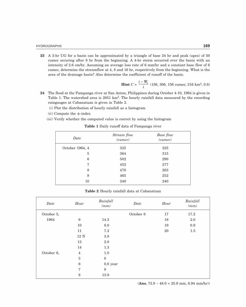
C-9\N-HYDRO\HYD5-3.PM5 169
HYDROGRAPHS 169
23 A 3-hr UG for a basin can be approximated by a triangle of base 24 hr and peak (apex) of 50cumec occuring after 8 hr from the beginning. A 4-hr storm occurred over the basin with anintensity of 2.6 cm/hr. Assuming an average loss rate of 6 mm/hr and a constant base flow of 6cumec, determine the streamflow at 4, 8 and 16 hr, respectively from the beginning. What is thearea of the drainage basin? Also determine the coefficient of runoff of the basin.
Hint C = i W
ii−
(156, 306, 156 cumec; 216 km2; 0.8)
24 The flood at the Pampanga river at San Anton, Philippines during October 4-10, 1964 is given inTable 1. The watershed area is 2851 km2. The hourly rainfall data measured by the recordingraingauges at Cabanatuan is given in Table 2.
(i) Plot the distribution of hourly rainfall as a histogram
(ii) Compute the φ–index
(iii) Verify whether the computed value is correct by using the histogram
Table 1 Daily runoff data of Pampanga river
DateStream flow Base flow
(cumec) (cumec)
October 1964, 4 325 325
5 364 315
6 502 290
7 452 277
8 470 263
9 465 252
10 240 240
Table 2 Hourly rainfall data at Cabanatuan
Date HourRainfall
Date HourRainfall
(mm) (mm)
October 5, October 6 17 17.2
1964 9 14.3 18 2.0
10 8.0 19 0.9
11 7.2 20 1.5
12 N 3.8
13 2.0
14 1.3
October 6, 4 1.0
5 0
6 0.8 year
7 0
8 13.9
(Ans. 73.9 – 48.0 = 25.9 mm, 6.94 mm/hr))

C-9\N-HYDRO\HYD5-3.PM5 170
170 HYDROLOGY
25 Storm rainfalls of 4.5 and 8 cm occurred over an area of 3750 km2 on July 10 and 11, respectivelyin a certain year. The loss rate can be assumed as 2.5 and 2 cm for the two days, respectively.The distribution percentage for the successive days are 20, 40, 15, 12, 8, 4 and 1. Determine thestreamflows for the successive days in cumec, assuming a base flow of 40 cumec for the first 2days, 80 cumec for the next 2 days, 60 cumec for further 2 days and 40 cumec for the subsequentdays. State the peak flood and the date of its occurence.
26 The flood water level (river stage H) since commencement of a 4-hr storm on a 2200 km2 basin isgiven below. Derive and sketch a 4-hr UH (unit is 1 cm), assuming a constant base flow of 9cumec.
Time (hr): 0 2 4 6 8 10 12 14 16 18 20 22
Stage, H(m): 0.5 3.0 4.5 4.6 4.3 3.3 2.8 2.2 1.9 1.2 1.0 0.5
Stage-discharge relation : Q = 100 (H–0.2)2, Q in cumec.
(Ans. Pnet = 2.86 cm; UHO: 0, 271, 644, 674, 585, 333, 233, 166, 98, 32, 19, 0, cumec)
27 Using the lag time of the SUH obtained in problem 16, for the sub-catchment of Ramganga(A = 323.5 km2) develop a 8 hr–UG by SCS method, given (pk = peak) :
ttpk
: 0.5 1 2 3 4 5
QQp
: 0.4 1 0.32 0.075 0.018 0.004
28 In a stream the base flow is observed to be 30 cumec on July 14, and 23 cumec on July 23.Estimate the base flow on August 10, and ground water storage on July 14 and August 10.
(Ans. Q (28 days) = 13.5 cumec; 88, 40 Mm3)
29 An agricultural watershed was urbanised over a period of 30 years. The rainfall loss was9 mm/hr before urbanisation, which dropped to 4 mm/hr after urbanisation. The 1-hr UG (unit1 cm) of this watershed can be assumed as a triangle of base 12 hr and height 160 cumec after 4hr before urbanisation and of base 8 hr and height 240 cumec after 3 hr, after urbanisation.
(a) Determine the area of the watershed.
(b) Draw the flood hydrograph after urbanisation for a storm of intensity 19 mm/hr for 1 hr and29 mm/hr in the next hour. Assume a uniform loss rate and a constant base flow of 10 cumec.
(c) Compute the coefficient of runoff before and after urbanisation.
(Ans. A = 346 km2, C = 0.67, 0.83]
Note The triangular areas of both the UG’s are same.

6.1 METHODS OF MEASURING STREAM FLOW
The most satisfactory determination of the runoff from a catchment is by measuring thedischarge of the stream draining it, which is termed as stream gauging. A gauging station isthe place or section on a stream where discharge measurements are made. Some of the usualmethods of stream gauging are given below:
(a) Venturiflumes or standing wave flumes (critical depth meter) for small channels.(b) Weirs or anicuts: Q = CLH3/2 ...(6.1)
where Q = stream discharge, C = coefficient of weir, L = length of weir (or anicut), H = head(depth of flow) over the weircrest
(c) Slope-area method: Q = AV ...(6.2)
V = C RS —Chezy ...(6.2 a)
V = 1n
R2/3 S1/2 —Manning ...(6.2 b)
Chezy’s C = 1n
R1/6, R = AP
...(6.2 c)
where C = Chezy’s constantN = Manning’s coefficient of roughnessR = hydraulic mean radiusA = cross-sectional area of flowP = wetted perimeterS = water surface slope (= bed slope)The cross-sectional area A is obtained by taking soundings below the water level at
intervals of, say, 6 m and plotting the profile of the cross-section and drawing the high floodlevel or water surface level.
The water surface slope is determined by means of gauges placed at the ends of thereach, say 1 km upstream of the gauging station and 1 km downstream of the gauging station(in a straight reach; if ∆h is the difference in water levels in a length L of the reach, then
S =∆hL
. The slope may also be determined by means of flood marks on either side and their
subsequent levelling.
STREAM GAUGING
171
Chapter 6

C-9\N-HYDRO\HYD6-1.PM5 172
172 HYDROLOGY
Careful notes on the nature of bed and banks, vegetation etc. should be made and ifpossible a photograph may be taken. From this, the constants C (Chezy’s) and n (Manning’s)can be found from the Tables.
The slope-area method is often used to estimate peak floods where no gauging stationexists.
(d) Contracted area methods:The drop in water surface in contracted sections as in bridge openings (see Fig. 6.15),
canal falls etc. is measured and the discharge is approximately given by
Q = Cd A1 2g h ha( )∆ + ...(6.3)where Cd = coefficient of discharge
A1 = area of the most contracted section∆h = difference in water surface between the upstream and down stream ends (of the
pier)ha = head due to the velocity of approach.
(e) Sluiceways, spillways and power conduits. The flow through any of the outlets in adam or the sum of the flows through these gives the discharge at any time.
(f) Salt-concentration method. The discharge is determined by introducing a chemical,generally common salt, at a known constant rate into flowing water and determining the quan-tity of chemical in the stream at a section downstream sufficiently distant to ensure thoroughmixing of the chemical with water. The discharge.
Q = c cc c
−−
2
2 1 q ...(6.4)
where q = quantity of solution injected (cc/sec) c = amount of salt in dosing solution (gm/cc) c1 = concentration of salt originally (before dosing) in the stream (gm/cc) c2 = concentration of salt in the sample downstream (gm/cc)This method is best suited for turbulent waters as the turbulence helps in thorough
mixing of the chemical; this is a costly process.(g) Area-velocity methods: Q = AVThe area of cross-section of flow may be determined by sounding and plotting the profile.
The mean velocity of flow (V) may be determined by making velocity measurements. The velocitydistribution in a cross-section and in a vertical in a stream are shown in Fig. 6.1 (a) and (b) andas such the methods of velocity measurements are as follows:
Velocity measurements from
Floats surfacesub-surface
measure surface velocity ;0.85
Velocity rods measure mean velocity,
Current meterPigmy
PropellerPrice
measure mean velocity in astrip of cross-section by
{ } vV v
V
s
s≈
RS|T|
UV|W|
R
S
||||
T
||||
...(6.5)
(i) one point method V = v0.6d ...(6.6 a)
(ii) two points method V = v vd d0.2 0.8
2+
(d = mean depth in the strip) ...(6.6 b)
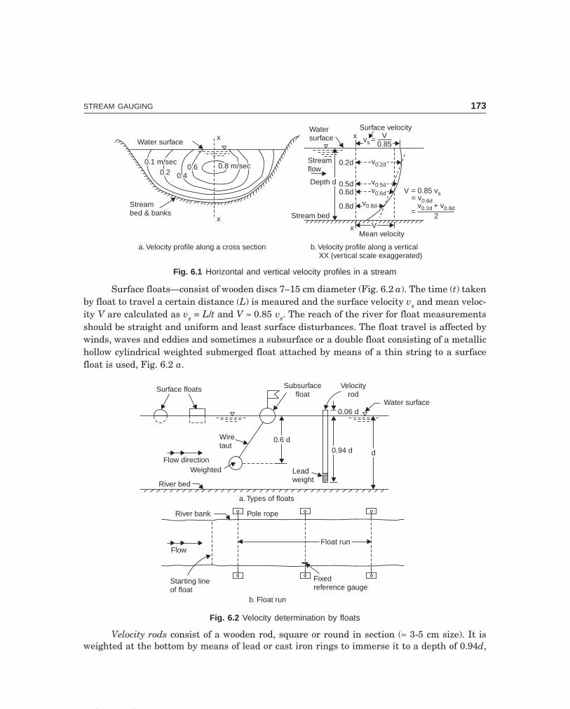
C-9\N-HYDRO\HYD6-1.PM5 173
STREAM GAUGING 173
Water surfacex
x
Streambed & banks
0.1 m/sec0.1 m/sec0.20.2 0.40.4
0.60.6 0.8 m/sec0.8 m/sec
Watersurface
Surface velocityx vs = V
0.85
Streamflow
Depth dDepth d
0.2d
0.5d0.6d
0.8d
v0.2dv0.2d
v0.5dv0.5dv0.6dv0.6d
v0.8dv0.8d
Stream bedVVx
Mean velocity
= 0.85 v= v
=
s0.6d
v2
0.2d + v0.8d
V
a. Velocity profile along a cross section b. Velocity profile along a verticalXX (vertical scale exaggerated)
Fig. 6.1 Horizontal and vertical velocity profiles in a stream
Surface floats—consist of wooden discs 7–15 cm diameter (Fig. 6.2 a). The time (t) takenby float to travel a certain distance (L) is meaured and the surface velocity vs and mean veloc-ity V are calculated as vs = L/t and V ≈ 0.85 vs. The reach of the river for float measurementsshould be straight and uniform and least surface disturbances. The float travel is affected bywinds, waves and eddies and sometimes a subsurface or a double float consisting of a metallichollow cylindrical weighted submerged float attached by means of a thin string to a surfacefloat is used, Fig. 6.2 a.
a. Types of floats
Surface floats Subsurfacefloat
Velocityrod
Water surface0.06 d
0.94 d0.94 d dd
0.6 d0.6 dWiretaut
Flow direction
River bed
Weighted Leadweight
b. Float run
Fixedreference gauge
Float runFloat run
Pole ropeRiver bank
Flow
Starting lineof float
Fig. 6.2 Velocity determination by floats
Velocity rods consist of a wooden rod, square or round in section (≈ 3-5 cm size). It isweighted at the bottom by means of lead or cast iron rings to immerse it to a depth of 0.94d,

C-9\N-HYDRO\HYD6-1.PM5 174
174 HYDROLOGY
where d is the depth of stream, to give the mean velocity of flow (V). The rods are so weightedthat they float nearly vertical with about 3–5 cm projecting above the water surface, so thatthey can be seen floating. A number of rods are required to suit the varying depths of cross-section.
At the beginning of the gauge run, a surface or rod float is released at the centre of acompartment (Fig. 6.2 b). The time taken for the float to reach the end of the gauge run (of thesame compartment) is noted. Knowing the length of the gauge run, the velocity of flow isdetermined.
6.2 CURRENT METER GAUGINGS
The current meter is an instrument, which has a rotating element which when placed in flow-ing water, the speed of revolutions has a definite relation with the velocity of flow past theelement. There are three types of current meters—(i) pigmy current meter, whose cup vaneassmbly is about 5 cm in diameter and is used for measuring velocities in streams of depth 15cm or less, (ii) the cup type, which consists of a wheel with conical cups revolving on a verticalaxis, and (iii) the screw or propeller type consisting of vanes revolving on a horizontal axis.Price, Ellis, Ottwatt meters are of vertical axis type while Off and Haskel, Amslar, Ott andAerofoil meters are of horizontal axis type. The Price meter is regarded as a universal meterand is equipped with a pentahead, a device for indicating every fifth revolution. The metermay be used for velocities from 1 to 4.5 m/sec in depths of 1-15 m from a boat, bridge, cable orwading. A counter weight (stream lined) is fixed below the meter to prevent it from swaying,Fig. 6.3.
Rod
Tail vane
Suspensioncable
Connectionto ear phone
Flow
Funnels onvertical axis
Counter weight
Fig. 6.3 Price current meter
Rating of the Current MeterThe relationship between the revolutions per second (N, rps) of the meter and the velocity offlow past the meter (v, m/sec) has to be first established, or if the rating equation is given bythe maker, it has to be verified. This process of calibration of the meter is called rating of thecurrent meter. The rating equation is of the form
v = aN + b ...(6.7)where a and b are constants (determined from rating of the current meter).

C-9\N-HYDRO\HYD6-1.PM5 175
STREAM GAUGING 175
The rating is done in a masonry tank of approximate dimensions 90 m × 2.4 m × 2.1 m,Fig. 6.4. The meter is towed in still water in the tank either by a pushing trolley (from whichthe meter is suspended) by men specially trained for the purpose or by an electric motor tomove the trolley at a constant speed on a track by the side of the tank, the distances beingpainted in m and cm in enamel on the track. A metronome adjusted to give ticks at every 2, 3,4, 5, 6, 7, 8, 10 sec is kept on the trolley. The men pushing the trolley would have been trainedto put paces uniformly to synchronise with the ticking of the metronome. When motorisedspeeds are adjusted to give different velocities. A cantilever beam is fixed to the trolley suchthat the projecting end is at the centre of the rating tank from which the meter is hung from asuspension rod. The meter should be immersed about 1 m below the water surface duringrating. The observer sits in the trolley, notes the time and distance traversed by the trolley fora fixed number of revolutions made by the meter (say, 10-100 depending on the speed). Thisoperation is repeated for different pushing velocities of the trolley. A current meter ratingcurve is drawn as ‘pushing velocity vs. rps’, which plots a straight line and the constants a andb are determined as shown in Fig. 6.5.
Current metertowedHanger
Still water
Rating tank: 90 × 2.4 × 2.1 m
Rails
MetronomeMoving trolley
3 6 9 12 15 18 21 24 27 30 33 36 39 42 45 48 51 54 57 60 63 66 69 72 75
Distances painted
a. Plan
Moving trolley
Current metertowed in still water
b. Cross section
Fig. 6.4 Current meter rating tank
Dy
Dx
DyDx
a =
Slope
Rating curvev = aN + b
b = intercept
Rev/sec of meter (N)
Pus
hing
velo
city
, or
mot
orsp
eed
v(m
/sec
) v =
or = Speed of motor
distance towed (m)time (sec)
Fig. 6.5 Current meter rating curve
Stage-Discharge-Rating CurveOnce the rating equation of the current meter is known, actual stream gauging can be donefrom bridges, cradle, boat or launch. The cross section of the stream at the gauging site isdivided into elemental strips of equal width b and the current meter is lowered to a depth of0.6 d below water surface in shallow depths (one-point method) and to depths of 0.2d and 0.8d

C-9\N-HYDRO\HYD6-1.PM5 176
176 HYDROLOGY
(two-points method) in deep waters, at the centre of each strip, Fig. 6.6. The mean depth (d) atthe centre of each strip is determined by sounding. The revolutions made by the meter in aknown time at the appropriate depths are noted by an ear phone (connected through a wire tothe penta or monocounter of the meter and the other to a dry cell) from which the velocities atthe appropriate depths are determined from the rating equation, Eq. (6.7).
bb bb bb bb
Cabledrum
Crabwinch
Pulley steel cable
Steel trestleLeft bank
0.6d
Hand propeller
Pulley
Cable carRight bank
Pulley
High water level
Stream bed
Elemental stripsof width (b)
.8d.8d.8d.8d
.2d
Depth (d)by sounding
Current meterlowered at 0.8d
Q = QS D
.6dAnchor
Masonryfoundation
Currentmeter positions
DQ (Strip) = (b.d)v + v
2.2d .8d
DQ (end strips) = (b.d) v.6d
or
0.6d0.6d
C
Fig. 6.6 Current meter gauging
It may be noted that the mean velocity is taken as that at 0.6d below water surface inshallow water (one-point method), and as the average of the velocities at 0.2d and 0.8d belowthe water surface (two-point method) in deep waters, as can be seen from the velocity distribu-tion in a vertical in a stream section, Fig. 6.1 (b). The discharge in each elemental strip isdetermined and the discharge in the stream is the sum of the discharges in all the elementalstrips.
There are two methods of determining the discharge in each elemental strip:(i) Mid-section method. In this method, the vertical in which the velocity measure-
ments are made (by one-point or two-points method) is taken as the middle of the strip, andthe water depth (d) in the vertical (determined by sounding) is taken as the mean depth of thestrip, Fig. 6.7 (a). If b is the width of strip (usually same for all strips) then the discharge in theelemental strip is given by
∆Q = (bd) v0.6d in shallow strips ...(6.8)
∆Q = (bd) × v vd d0.2 0.8
2+
in deep water strips ...(6.8 a)
stream discharge, Q = Σ ∆Q ...(6.8 b)In this method, the discharge in the two-triangular bits near the ends are not included
in the discharge computation.

C-9\N-HYDRO\HYD6-1.PM5 177
STREAM GAUGING 177
bb bb bb bb bb bb
L.B.
M d1d1
d2d2 d3d3d4d4
d5d5
d6d6N
Currentmeterlocations Verticals for
mean depth andmean velocity
R.B.
D Ds or M & N notincluded incomputation ofdischarge
DQ (Strip) = (b.d)or
= (b.d) v.6d
v + v.2d .8d
2
a. Mid-section method
L.B. R.B.
bb bb bb bb bb bb bb
12
3 45
6
7d1d1
d2d2 d3d3
d4d4
d5d5
d6d6
dmdmvmvm
Mean sectionsof strips Strips 1-7 DQ (Strip) = (b.d ) vm m
dm = ,
(for strip 3)
d + d2
2 3 vm =v +
22 3v
b. Mean-section method
Q = QS D
Fig. 6.7 Mid-section and Mean-section methods
(ii) Mean-section method. In this method, the elemental strip is taken between two ver-ticals and the mean depth is taken as the average of the depths in the two verticals (deter-mined by sounding). The width of the strip is distance b between the two verticals. The velocityin the strip is taken as the average of the mean velocity determined in the two verticals (byone-point or two-points method), Fig. 6.7 (b). The discharge in the elemental strip is given by
Q = b d d V V1 2 1 2
2 2+F
HGIKJ
+FHG
IKJ ...(6.9)
V1, V2 determined as v0.6d in shallow strip
andv vd d0.2 0.8
2+
in deep water strip ...(6.9 a)
Stream discharge, Q = Σ ∆Q ...(6.9 b)
The mean section method is considered to be slightly more accurate, but the mid-sectionmethod is faster and is generally used.Example 6.1 The following data were collected for a stream at a gauging station. Compute thedischarge.

C-9\N-HYDRO\HYD6-1.PM5 178
178 HYDROLOGY
Distance from depth, d Immersion of current meterone end of (m) below water surface
water surface at 0.6d at 0.2d at 0.8d
(m) Rev. Sec. Rev. Sec. Rev. Sec.
3 1.4 12 50
6 3.3 38 52 23 55
9 5.0 40 58 30 54
12 9.0 48 60 34 58
15 5.4 34 52 30 50
18 3.8 35 52 30 54
21 1.8 18 50
Rating equation of current meter: v = 0.3 N + 0.05, N = rps, v = velocity, (m/sec), Rev.-Revolutions, Sec-time in seconds.
Solution The discharge in each strip, ∆Q = (bd) V, where V is the average velocity in eachstrip, Fig. 6.8. In the first and the last strips (near the banks) where the depth is shallow,
V = v0.6 d, and in the other five intermediate strips (with deep water), V = v vd d0.2 0.8
2+
. Width of
each strip, b = 3 m, mean depth of strip = d, and the total discharge, Q = Σ ∆Q = 20.6 cumec,as computed in Table 6.1.
Not considered7 Elemental strips (b = 3 m)
Not considered
L.B3
m3
m3
m3
m3
m3
m3
m3
m3
m3
m3
m3
m3
m3
m3
m3
m
3m
3m
3m
3m
3m
3m
3m
3m
3m
3m
3m
3m
3m
3m
1
2 3 4 5 6 7
1.4m
3.3m 5.0
m9.0m
5.4m
3.8m
1.8m
Meter locationat 0.6dMeter location
at 0.6 d
Meter locationsat 0.2d & 0.8d
in vertical
V in vertical
= (V + V ) or V
mean
0.2d 0.8d 0.6d12
Q = Q = (b.d) Vå å meanÑ7
1
1
1
R.B0
21 m
Fig. 6.8 Discharge computation (Example 6.1)
6.3 STAGE-DISCHARGE-RATING CURVE
A river is gauged by current meter throughout the rainy season (for about 3 months) at differentstages (water levels) of the river. The water stage can be read on the enamel painted staffgauges (gauge posts) erected at different levels at a gauging station Fig. 6.9; it may be notedthat corresponding graduation of gauge posts at two locations are fixed at the same level. Acurve is drawn by plotting ‘stream discharge ‘Q vs. gauge height h’ which is called the ‘stage-discharge rating curve’ as shown in Fig. 6.10. From this rating curve, the stream discharge

C-9\N-HYDRO\HYD6-1.PM5 179
STREAM GAUGING 179D
ista
nce
fro
mD
epth
, dIm
mer
sion
of
curr
ent
met
er b
elow
wat
er s
urf
ace
Ave
rage
Dis
char
ge i
n s
trip
one
end
of
(m)
dep
th =
xd
Rev
.ti
me
N =
R/t
v =
0.3
N +
0.0
5ve
loci
ty∆Q
= (
bd)
V
wat
er s
urf
ace
(x =
0.6
, 0.2
, 0.8
)R
(sec
.)(r
ps)
(m/s
ec)
in s
trip
b =
3m
(m)
(m)
V (
m/s
ec)
31.
40.
8412
500.
240.
122
0.12
20.
51
63.
30.
6638
520.
730.
269
0.22
3*2.
16
2.64
2355
0.42
0.17
6
95.
01.
0040
580.
690.
257
0.23
63.
54
4.00
3054
0.56
0.21
8
129.
01.
8048
600.
800.
290
0.25
97.
00
7.20
3458
0.59
0.22
7
155.
41.
0834
520.
650.
245
0.23
83.
85
4.32
3050
0.60
0.23
0
183.
80.
7635
520.
670.
251
0.23
42.
68
3.04
3054
0.56
0.21
8
211.
81.
0818
500.
360.
158
0.15
80.
86
Tot
al
Q =
20.
60 c
um
ec
* 0
269
017
62
..
+ =
0.2
23.
Tab
le 6
.1 C
urr
ent
met
er g
augi
ng
of R
iver
. (E
xam
ple
6.1)

C-9\N-HYDRO\HYD6-1.PM5 180
180 HYDROLOGY
corresponding to staff gauge readings taken throughout the year/s can be obtained, as long asthe section of the stream at or near the gauging site has not materially altered. Periodicalgaugings (say, once in three years) are conducted to verify the rating curve, or to revise therating curve if any change in section has been noticed.
5.0
7.5m
Staff gauges(enamel painted)
5.0m
High water level
2.5m
2.5
Streambank
Flow Q (cumec)
River bed ho
Staff reading(Gauge height, h)
Staff reading(Gauge height, h)
Fig. 6.9 Gauge posts on river bank
Stage-dischargerating curve
Log-log paper
Staff guage reading 0.7 m
Discharge20 cumec
1086
43
2
1.0.8.6
.4
.3
.2
0.11 2 3 4 6 8 10 20 30 50 70 100 200 400 600 1000
Stream discharge, Q (cumec)
Gau
gehe
ight
(hm
)
Fig. 6.10 Stage-discharge rating curve
For a continuous record of water stage (gauge heights or readings) during floods, anAutomatic Water Stage Recorder (AWLR) is installed inside a gauge well on one of the banksof the stream at the gauging site, connected to the stream at different levels by pipes, Fig. 6.11.A steel wire rope with a float at one end and a counter weight at the other passes over a pulleyconnected to a cylindrical drum over which a chart is wrapped. The rise and fall of the floatwith the water level causes rotation of the drum while a clock mechanism moves a pen axiallyalong the drum, thus producing a water stage hydrograph. The time scale on the graph isusually so chosen as to cover a week’s period. Thus, a continuous record of the river stage withthe time is obtained. The water level in well is not subject to fluctuations caused by wind orwaves.
If the river is subject to scour, the well should be sufficiently deep and the zero of thegauge should be sufficiently below the bed, so that the water surface will not come below the
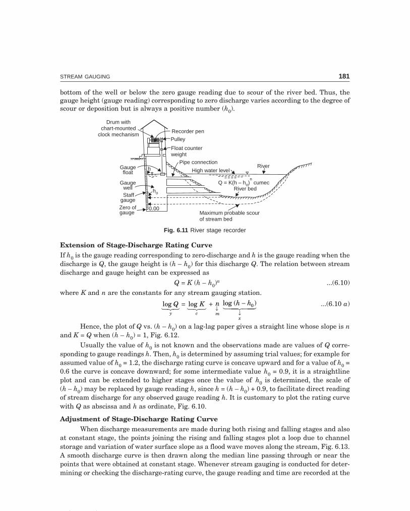
C-9\N-HYDRO\HYD6-1.PM5 181
STREAM GAUGING 181
bottom of the well or below the zero gauge reading due to scour of the river bed. Thus, thegauge height (gauge reading) corresponding to zero discharge varies according to the degree ofscour or deposition but is always a positive number (h0).
hGaugefloat
GaugewellStaff
gaugeZero ofgauge
Drum withchart-mounted
clock mechanismRecorder pen
Pulley
Float counterweight
Pipe connection
High water level
Maximum probable scourof stream bed
River
Q = K(h – h ) cumecon
River bedho
0.00
Fig. 6.11 River stage recorder
Extension of Stage-Discharge Rating CurveIf h0 is the gauge reading corresponding to zero-discharge and h is the gauge reading when thedischarge is Q, the gauge height is (h – h0) for this discharge Q. The relation between streamdischarge and gauge height can be expressed as
Q = K (h – h0)n ...(6.10)
where K and n are the constants for any stream gauging station.
log logQ Ky c
��� ���= + n
mB
log ( )h h
x
−B
0� ��� ��� ...(6.10 a)
Hence, the plot of Q vs. (h – h0) on a lag-lag paper gives a straight line whose slope is nand K = Q when (h – h0) = 1, Fig. 6.12.
Usually the value of h0 is not known and the observations made are values of Q corre-sponding to gauge readings h. Then, h0 is determined by assuming trial values; for example forassumed value of h0 = 1.2, the discharge rating curve is concave upward and for a value of h0 =0.6 the curve is concave downward; for some intermediate value h0 = 0.9, it is a straightlineplot and can be extended to higher stages once the value of h0 is determined, the scale of(h – h0) may be replaced by gauge reading h, since h = (h – h0) + 0.9, to facilitate direct readingof stream discharge for any observed gauge reading h. It is customary to plot the rating curvewith Q as abscissa and h as ordinate, Fig. 6.10.
Adjustment of Stage-Discharge Rating CurveWhen discharge measurements are made during both rising and falling stages and also
at constant stage, the points joining the rising and falling stages plot a loop due to channelstorage and variation of water surface slope as a flood wave moves along the stream, Fig. 6.13.A smooth discharge curve is then drawn along the median line passing through or near thepoints that were obtained at constant stage. Whenever stream gauging is conducted for deter-mining or checking the discharge-rating curve, the gauge reading and time are recorded at the

C-9\N-HYDRO\HYD6-1.PM5 182
182 HYDROLOGY
beginning and at the end of the gauging to calculate the rate of change in stage. Curves-relating percentage correction to discharge and rate of change in stage can be obtained fromcontinuous discharge measurement during rising, falling and constant stages of the river.
1000800
600
400
300
200
150
10080
60
40
30
20
15
108
654
3
2
1.5
1
Dis
char
ge,Q
(cum
ec)
0.1 .15 .2 .3 .4 .6 .81.0 1.5 2 3 4 6 8 10 15 20 30 40 60 80100
1.0 1.1 1.2 1.4 1.6 1.9 2.9 4.9 6.9 10.9 20.9 40.9Gauge reading h (m)
Lag-lag paper
Q = 240 cumec Q = 1.2 (h-0.9)2.2
(h – h ) = 1oK = Q = 1.2
= 3.6 cm
h=
1.2
o
h=
0.6
oC
onca
veup
war
d
Con
cave
upw
ard
Con
cave
dow
nwar
d
Con
cave
dow
nwar
dÑÑ
y = 7.92 cmy = 7.92 cm
Stra
ight
line
Stra
ight
line
0.9
0.9
12 m = h
Slope n = = = 2.2of st. lineSlope n = = = 2.2of st. line
ÑÑyxyx
Ñ 7.923.607.923.60
h=
oh=
oQ = 25.3 cumec
(h – h ) mo
Ñx
Fig. 6.12 Extension of stage-discharge-rating curve (Example 6.2)
Correction has to be applied for the discharge obtained from the rating curve during arising or falling stage i.e., during a flood. For this purpose, an auxiliary gauge is establishedsome distance upstream or downstream from the main gauge (Fig. 6.14). If Q0 is the dischargewhen ∆h0 is the difference of gauge readings between the main and auxiliary gauges duringnormal flow, and Qa is the discharge when ∆ha is the difference of the two gauges during arising or falling stage then
a
0 =
∆∆
hh
an
0
FHG
IKJ ...(6.11)
where the exponent n ≈ 0.5, since Q varies as the square root of the energy gradient, which inturn varies with ∆h, the distance between the gauges being constant.

C-9\N-HYDRO\HYD6-1.PM5 183
STREAM GAUGING 183
Uniform flow ratingcurve (median line)
Rising sta
geFalling sta
ge
Wat
erst
age
h(m
)
Discharge Q (cumec)
Fig. 6.13 Adjustment of flow rating curve
Water surface
Main gauge
Auxiliary gauge
Rising stage
Normal stage
Falling stage
Ñha ÑÑ
hoho
FlowStream bed
hh
a
o
ÑÑQ = Qa o
n
n = 0.5
Fig. 6.14 Auxiliary gauge for flow adjustment
From Eq. (6.11) the actual discharge Qa during a rising or falling stage can be deter-mined. The distance between the two gauges should be such that ∆h0 is at least 0.3 m, to avoidobservational errors.
6.4 SELECTION OF SITE FOR A STREAM GAUGING STATION
The following factors have to be considered in selecting a site for a stream gauging station.(i) The section should be straight and uniform for a length of about 10 to 20 times the
width of the stream.(ii) The bed and banks of the stream should be firm and stable so as to ensure consist-
ency of area-discharge relationship, i.e., the cross section should not be subjected to change by

C-9\N-HYDRO\HYD6-1.PM5 184
184 HYDROLOGY
silting or scouring, during different stages of flow; a smooth rock, shingle or clay bed is favour-able, while a fine sandy bed is unfavourable.
(iii) The bed and banks should be free from vegetal growth, boulders or other obstruc-tions like bridge piers, etc.
(iv) There should be no larger overflow section at flood stage. The best cross section isone with V-shape, so that there is sufficient depth for immersing the current meter withoutbeing affected by the bed roughness of the stream.
(v) The part of the reach having the most regular transverse section and steady flowwith the current normal to the metering section and velocities in the range of 0.3–1.2 m/secshould be selected.
(vi) To ensure consistency between stage and discharge, there should be a good controlsection far downstream of the gauging site. This control may be in the form of steep rapids,large rocky boulders, restricted passages, crest of weirs or anicuts etc.
(vii) The sites above the confluence of rivers are best avoided if the flow is affected byback water conditions due to the varying discharges in the tributaries.
(viii) The stream gauging station should be easily accessible.Example 6.2 The stream discharges for various stages at a particular section were observed tobe as follows. Obtain an equation for the stage-discharge relationship and determine the dis-charge for a stage of 4.9 m and 12 m.
Stage (m) 1.81 2.00 2.30 2.90 3.70 4.50
Discharge (cumec) 1.00 1.50 2.55 5.60 11.70 20.20
Stage (m) 5.40 6.10 7.30 7.70 8.10
Discharge (cumec) 32.50 44.50 70.0 80.0 90.0
Solution The relation between the stage (h) and discharge (Q) of the stream can be assumedof the form
Q = K (h – a)n, (similar to Eq. (6.10)where K, a and n are the constants. Plot Q vs. (h – a) on a lag-lag paper assuming a value forthe constant a = 0.6 m (say); the curve obtained is concave downwards, Fig. 6.12. Now assumea value a = 1.2 m (say) and the curve obtained is concave upward. Now try an intermediatevalue a = 0.9 m, which plots a straight line and represents the stage discharge relationship.The slope of this straight line gives the value of the exponent n = 2.2, and from the graph forh – a = 1, Q = 1.2 = K. Now the constants are determined and the equation for the stage-discharge relationship is
Q = 1.2 (h – 0.9)2.2
It may be noted that the value of a = 0.9, which gives a straight line plot is the gaugereading for zero discharge. Now the abscissa of (h – a) may be replaced by the gauge reading(stage) h, by adding the value of ‘a’ to (h – a) values. For example the (h – a) values of 0.1, 1, 2,4, 6, 8 and 10 may be replaced by the h values of 1, 1.9, 2.9, 4.9, 6.9, 8.9 and 10.9 respectively.Now for any gauge reading (stage) h, the discharge Q can be directly read from the graph andthe stage discharge curve can be extended. From the graph, Fig. 6.12,
for h = 4.9 m, Q = 25.3 cumec
C-9\N-HYDRO\HYD6-1.PM5 185
STREAM GAUGING 185
and for h = 12.0 m, Q = 240 cumecwhich can be verified by the stage-discharge equation obtained as
for h = 4.9 m, Q = 1.2 (4.9 – 0.9)2.2 = 25.3 cumecfor h = 12 m, Q = 1.2 (12 – 0.9)2.2 = 240 cumecNote The equation for the stage-discharge relation can also be obtained by ‘Linear Regression’
by assuming trial values of ‘a’ and computer-based numberical analysis. See chapter—13.
Example 6.3 The following data were obtained by stream gauging of a river:Main gauge staff reading (m) 12.00 12.00Auxiliary gauge staff reading (m) 11.65 11.02Discharge (cumec) 9.50 15.20
what should be the discharge when the main gauge reads 12 m and the auxiliary gauge reads11.37 m?Solution ∆h0 = 12.00 – 11.65 = 0.35 m
∆ha = 12.00 – 11.02 = 0.98 m
Eq. (6.10): QQ
hh
a an
0 0=FHG
IKJ
∆∆
15 209 50
0 980 35
..
.
.= FHG
IKJ
n
∴ n = 0.5125Again, when the auxiliary gauge reads 11.37 m,
∆ha = 12.00 – 11.37 = 0.63 m
Qa
9 500 630 35
0.5125
...
= FHG
IKJ
∴ Qa = 12.85 cumecExample 6.4 A bridge has to be constructed over a river, which receives flow from three branchesabove the site. Compute the maximum flood discharge at the bridge site from the followingdata:Branch 1 has a bridge:
Width of natural water way 324.0 mLineal water way under the bridge(with Cd = 0.95 for rounded entry) 262.5 mDepth upstream of bridge 4.6 mDepth downstream of bridge 2.8 m
Branch 2 has a catchment area of 4125 km2
Ryve’s C = 10Branch 3 levelling of cross section (c/s) data:
Distance from BM (m) 0 11 24 52 67 79 84RL on c/s (m) 10.8 9.6 4.2 2.4 5.4 10.2 10.5Levelling of longitudinal-section (L/S) data:
Distance from 1 km at 1 kmbridge site upstream bridge site downstream
HFL along L/S (m) 9.60 9.0 8.39Manning’s n may be assumed at 0.03.

C-9\N-HYDRO\HYD6-1.PM5 186
186 HYDROLOGY
Solution (i) Discharge from Branch 1, i.e., Q1 under bridge openings, Fig. 6.15, from Eq. (6.3)
Q1 = Cd A1 2g h ha( )∆ +If L, d, V and L1, d1, V1 refer to the length, mean depth and velocity of the normal
stream (upstream of bridge site) and those under the contracted section of the bridge and also
A1 = L1d, Q1 = LdV, ha = V
g
2
2
Flowdd
Afflux hÑ
V
a. Cross section
Superstructure Parapet Lineal water wayL = 3L1
Abutment Abutmentll
MWLPiers
Foundation onhard rock
b. Flow through bridge openings
ll ll
Fig. 6.15 Flow through bridge openings (Example 6.4)
Eq. (6.3) after substitution and simplification yields the expression for afflux (i.e., head-ing up of water on the upstream face of the bridge openings) as
Afflux ∆h = V
gL
C Ld
2 2
2122
1−FHG
IKJ ...(6.12)
If the Branch 1, flow under bridge openings
4.6 – 2.8 = V 2 2
2 22 9 81324
0 95 262 51
× ×−
FHG
IKJ. . .
∴ V = 7.16 m/secQ1 = LdV = 324 × 2.8 × 7.16 = 6500 cumec
(ii) Discharge from Branch 2:From Ryve’s formula (see Eq. 8.2)
Q2 = CA2/3 ...(6.13) = 10 (4125)2/3 = 2580 cumec

C-9\N-HYDRO\HYD6-1.PM5 187
STREAM GAUGING 187
(iii) Discharge from Branch 3 (from slope-area method): See Table 6.2 for computationC/S area and wetted perimeter, Fig. 6.16.
Table 6.2 Computation C/S area and wetted perimeter (Fig. 6.16)
Area Area Area, A1 Wetted perimeter, P1no. shape (m2) (m)
1. 12 × 11.55 × 4.8 = 27.75 1155 4 82 2. .+ = 12.5
2. 12 (4.8 + 6.6) 28 = 159.60 28 182 2+ . = 28.2
3. 12 (6.6 + 3.6)15 = 76.50 15 32 2+ = 15.2
4. 12 × 9 × 3.6 = 16.20 9 3 62 2+ . = 9.7
A = 280.05 P = 65.6
1311.55
.6
4.8 281.8 3
9.0H.F.L. 1.2 1293.6
15
79 8410.2 10.9
675.4
522.4
244.2
119.610.8
0R.L.Dist.
Fig. 6.16 Cross section of river at bridge site (Example 6.4)
Hydraulic mean radius, R = AP
= 280 0565 6
.
. = 4.27 m
Water surface slope, S = ∆hL
= −×
=9 60 8 392 1000
11652
. .
By Manning’s formula, the velocity of flow
V = 1n
R2/3 S1/2 = 1
0 034 27
11652
2 3
.( . ) / 1/2 = 2.16 m/sec
∴ Q3 = AV = 280.05 × 2.16 = 605 cumecDischarge at bridge site
Q = Q1 + Q2 + Q3 = 6500 + 2580 + 605 = 9685 cumec
�������
I Choose the correct statement/s
The method of measuring discharge in a turbulent stream is
(i) by measuring the drop in water surface under bridge openings and canal falls.

C-9\N-HYDRO\HYD6-1.PM5 188
188 HYDROLOGY
(ii) by adding common salt into flowing water and determining its concentration downstream.
(iii) by slope-area method.
(iv) by area-velocity method.
(v) by measuring head over weirs or anicuts.
(vi) by measuring the upstream depth in a standing wave flume.
II Match the items in ‘A’ with the items in ‘B’
A B
(i) Area-velocity method (a) Afflux
(ii) Slope-area method (b) Turbulent streams
(iii) Bridge openings (c) Mean velocity
(iv) Salt-concentration method (d) v = aN + b
(v) Surface and subsurface floats (e) Q = K(h – a)n
(vi) Velocity rods (f) AWLR
(vii) Current-meter rating (g) Control section downstream
(viii) Stage-discharge curve (h) Peak flood where no gauging
station exists
(ix) River stage (i) Current-meter gauging
(x) Stream gauging spite (j) Surface velocity
III Say ‘true’ or ‘false’, if false, give the correct statement:
(i) The staff-gauge reading corresponding to zero-discharge in a stream is always a positivenumber.
(ii) The mean velocity in a vertical stream can be calculated by measuring the velocities at one-fifth and four-fifths of the depth of the stream in that vertical.
(iii) While the surface and subsurface floats measure the mean velocity of the stream, the veloc-ity rods measure the surface velocity.
(iv) Subsurface floats will not give the velocity accurately since they are affected by wind.
(v) Discharge in a river can not be determined by measurement near bridge openings.
(vi) The salt-concentration method can best be used to determine the discharge of non-turbulentrivers.
(vii) The hydraulic turbine can be used as a good water meter.
(viii) The stream gauging site should be on the upstream of the confluence of rivers.
(ix) There should be a good-control section immediately upstream of the gauging site.
(x) The calibration of the current meter is called the current meter rating while the stage-dis-charge is the relation between the staff-gauge reading and the stream discharge.
(xi) If the stage-discharge relation is governed by the slope, size and roughness of the channelover a considerable distance, the station is under channel control.
(xii) A pressure transducer may be used to obtain:
(a) a stage-hydrograph.
(b) a discharge–hydrograph.
(xiii) The slope-area method is often used to estimate peak floods near the existing gauging station.
(false: ii, iv, v, vi, viii, ix, xiii)

C-9\N-HYDRO\HYD6-1.PM5 189
STREAM GAUGING 189
�������
1 (a) What are the factors that influence the selection of a site for a stream gauging station?
(b) Explain how the stage-discharge-rating curve for a stream-gauging station is prepared. Sketcha typical rating curve. What are the sources of error in getting the discharge from the ratingcurve?
2 (a) What equipment will you use for making velocity measurements in a stream? Explain.
(b) Velocity measurements are to be made at a vertical in a stream. At what height or heightsfrom the bed, will you make the measurements to determine the mean in vertical velocity by:
(i) one-point method, and (ii) by two-points method?
3 (a) What is a flow rating curve’? Explain its use. Sketch a typical flow rating curve.
(b) Following velocities were recorded in a stream with a current meter.
Depth above bed (m): 0 1 2 3 4
Velocity (m/sec): 0 0.5 0.7 0.8 0.8
Find the discharge per unit width of stream near the point of measurement. Depth of flow atthe point was 5 m. (3.75 cumec)
4 (a) Explain briefly the method of stream gauging by area-velocity method.
(b) The following data were collected for a stream at a gauging station. Compute the dischargeby (i) mid-section method (ii) mean-section method.
Distance from one Depthend of water of Velocity (m/sec)
surface water at 0.6d at 0.2d at 0.8d(m) (m)
0 0 — — —
1.2 0.7 0.4 — —
2.4 1.7 0.7 0.5
3.6 2.5 0.9 0.6
4.8 1.3 0.6 0.4
6.0 0.5 0.35
7.2 0 — — —
(4.8, 4.442 cumec)
5 (a) Explain: ‘current metre rating curve’. How it is prepared ? Sketch a typical rating curve.
(b) What do you understand by the term ‘control point’ with reference to a stream gaugingstation?
6 The staff gauge readings and the corresponding discharges measured in a stream are givenbelow. Assuming the relationship to be exponential, fit an equation by drawing a graph. What isthe discharge for a staff gauge reading of 1.6 m and 2.5 m?
Gauge reading (m): 0.40 0.70 1.09 1.28 1.49 1.83 2.32
Discharge (cumec): 24 47 80 98 121 163 268
7 The following data were collected for two verticals in a stream at a gauging station. Compute thedischarge in the elemental strips by
(i) the mid-section method (ii) the mean-section method

C-9\N-HYDRO\HYD6-1.PM5 190
190 HYDROLOGY
Distance from Depth, d Immersion of current meterone end of (m) below water surface (m)
water surface at 0.2d at 0.8d
(m) rev sec rev sec
3 0.8 135 150 97 151
6 1.2 150 100 150 138
Rating equation of the current meter; v = 0.7 N + 0.03 where N = rev./sec, v = velocity (m/sec).
8 The following data are obtained from the current meter gauging of a stream, at a gauging sta-tion. Compute the stream discharge.
Distance from one Depth of water, d Immersion of current meterend of water surface (m) below water surface
(m) depth (m) rev sec
0 0 — — —
2 1.0 0.6 10 40
4 2.2 0.44 36 48
1.76 20 50
6 4.0 0.80 40 57
3.20 30 53
8 8.0 1.6 46 59
6.4 33 57
10 4.2 0.84 33 51
3.36 29 49
12 2.5 0.50 34 52
2.00 29 53
14 1.2 0.72 16 48
16 0 — — —
Rating equation of current meter: v = 0.2 N + 0.04, where N = rev./sec, v = velocity (m/sec).
9. A surface float took 10 sec to travel a straight run of a stream of 20 m. What is the approximatemean velocity of the stream? If a velocity rod had been used, what time it would have taken totravel the same run. (1.7 m/sec, 11.8 sec)
10. (a) What is the effect of rising or falling stage upon the discharge-curve?
(b) The following data are obtained by stream gauging of a river:
Main gauge staff reading (m) 9.6 9.6
Auxiliary gauge staff reading (m) 9.32 8.63
Discharge (cumec) 4.50 8.45
What should be the discharge when the main gauge reads 9.6 m and the auxiliary gauge reads9.02 m? (6.55 cumec)
11. Write a note on ‘stream gauging with shifting control’.

C-9\N-HYDRO\HYD6-1.PM5 191
STREAM GAUGING 191
12. The cross section (C/S) of a river is as follows:
Distance from BM (m) 0 10 20 30 40 50 60 70
Reduced level on C/S (m) 46.70 44.5 42.80 42.10 42.70 42.70 44.00 46.80
Longitudinal section (L/S) is as follows:
Distance (m) 1 km upstream at bridge site 1 km downstream
HFL along L/S (m) 45.10 44.50 43.89
Manning’s n may be assumed as 0.03.
A bridge is proposed across the river. Calculate the high flood discharge at bridge site.
13. A bridge is proposed across a stream which has a catchment area of 3200 km2. Ryve’s coefficientof C = 10 applies. Compute the maximum flood discharge at bridge site.
14. The following are the measurements at a bridge site, during floods. Compute the maximum flooddischarge at bridge site:
Width of natural water way 284 m
Lineal water way under the bridge 227 m
For rounded entry take Cd as 0.95
Depth upstream of bridge 4.80 m
Depth downstream of bridge 3.00 m

Chapter 7
7.1 TYPES OF AQUIFERS AND FORMATIONS
Ground water is widely distributed under the ground and is a replenishable resource unlikeother resources of the earth. The problems in Ground Water Investigation are the zones ofoccurrence and recharge. The modern trends are to create more opportunity for recharge ofground water from natural sources like rain, percolation dams, etc. The ground water is freefrom pollution and the ground water storage is free from atomic attacks. Ground water can bedeveloped at a small capital cost in least possible time, and intensive irrigation can be prac-tised with double and tripple cropping including commercial crops; ground water can be usedfor supplemental irrigation during periods of deficient surface supply, for the year-round irri-gation practice.
A water bearing geologic formation or stratum capable of transmitting water throughits pores at a rate sufficient for economic extraction by wells is called ‘aquifer’. Formations thatserve as good aquifers are:
• unconsolidated gravels, sands, alluvium• lake sediments, glacial deposits• sand stones• limestones with cavities (caverns) formed by the action of acid waters (solution open-
ings in limestones and dolomites)• granites and marble with fissures and cracks, weathered gneisses and schists• heavily shettered quartzites• vescicular basalts• slates (better than shales owing to their jointed conditions)A geologic formation, which can absorb water but can not transmit significant amounts
is called an ‘aquiclude’. Examples are clays, shales, etc.A geologic formation with no interconnected pores and hence can neither absorb nor
transmit water is called an ‘aquifuge’. Examples are basalts, granites, etc.A geologic formation of rather impervious nature, which transmits water at a slow rate
compared to an aquifer (insufficient for pumping from wells) is called an ‘aquitard’. Examplesare clay lenses interbedded with sand.
Specific yield. While porosity (n) is a measure of the water bearing capacity of the for-mation, all this water can not be drained by gravity or by pumping from wells as a portion ofwater is held in the void spaces by molecular and surface tension forces. The volume of water,
GROUND WATER
192

C-9\N-HYDRO\HYD7-1.PM5 193
GROUND WATER 193
expressed as a percentage of the total volume of the saturated aquifer, that will drain bygravity when the water table (Ground Water Table (GWT) drops due to pumping or drainage,is called the ‘specific yield (Sy)’ and that percentage volume of water, which will not drain bygravity is called ‘specific retention (Sr)’ and corresponds to ‘field capacity’ i.e., water holdingcapacity of soil (for use by plants and is an important factor for irrigation of crops). Thus,
porosity = specific yield + specific retention n = Sy + Sr ...(7.1)
Specific yield depends upon grain size, shape and distribution of pores and compactionof the formation. The values of specific yields for alluvial aquifers are in the range of 10–20%and for uniform sands about 30%.
7.2 CONFINED AND UNCONFINED AQUIFERS
If there is homogeneous porous formation extending from the ground surface up to an imper-vious bed underneath (Fig. 7.1), rainwater percolating down in the soil saturates the forma-tion and builds up the ground water table (GWT). This aquifer under water table conditions iscalled an unconfined aquifer (water-table aquifer) and well drilled into this aquifer is called awater table well.
Aquiclude(Impervious)
Aquiclude(Impervious)
Bed rockBed rock
Confined or artesianaquifer
Confined or artesianaquifer
22
Confininglayer
Confininglayer Water table
aquiferWater table
aquifer
W.T. AquiferW.T. Aquifer22
Imp layerImp layer
Cap. fringeCap. fringeGWTGWT
Sloping G.S. 11
W.T.W.T.
PrecipitationRecharge area at
outcropping of formation
Piezometricsurface
Flowing artesianwell
Water tablewell
Non-flowingartesian well
Perchedwater table
1 Zone of aeration2 Zone of saturation
Fig. 7.1 Types of aquifers and location of wells
On the other hand, if a porous formation underneath is sandwiched between two imper-vious strata (aquicludes) and is recharged by a natural source (by rain water when the forma-tion outcrops at the ground surface—recharge area, or outcrops into a river-bed or bank) at ahigher elevation so that the water is under pressure in the aquifer (like pipe flow), i.e., artesiancondition. Such an aquifer is called an artesian aquifer or confined aquifer. If a well is drilledinto an artesian aquifer, the water level rises in the well to its initial level at the rechargesource called the piezometric surface. If the piezometric surface is above the ground level atthe location of the well, the well is called ‘flowing artesian well’ since the water flows out of thewell like a spring, and if the piezometric surface is below the ground level at the well location,the well is called a non-flowing artesian well. In practice, a well can be drilled through 2-3artesian aquifers (if multiple artesian aquifers exist at different depths below ground level).

C-9\N-HYDRO\HYD7-1.PM5 194
194 HYDROLOGY
Sometimes a small band of impervious strata lying above the main ground water table(GWT) holds part of the water percolating from above. Such small water bodies of local naturecan be exhausted quickly and are deceptive. The water level in them is called ‘perched watertable’.
Storage coefficient. The volume of water given out by a unit prism of aquifer (i.e., acolumn of aquifer standing on a unit horizontal area) when the piezometric surface (confinedaquifers) or the water table (unconfined aquifers) drops by unit depth is called the storagecoefficient of the aquifer (S) and is dimensionless (fraction). It is the same as the volume ofwater taken into storage by a unit prism of the aquifer when the piezometric surface or watertable rises by unit depth. In the case of water table (unconfined) aquifer, the storage coefficientis the same of specific yield (Sy).
Since the water is under pressure in an artesian aquifer, the storage coefficient of anartesian aquifer is attributable to the compressibility of the aquifer skeleton and expansibilityof the pore water (as it comes out of the aquifer to atmospheric pressure when the well ispumped) and is given by the relation.
S = γwnb 1 1
K nEw s+
FHG
IKJ ...(7.2)
where S = storage coefficient (decimal) γw = specific weight of water n = porosity of soil (decimal) b = thickness of the confined aquiferKw = bulk modulus of elasticity of waterEs = modulus of compressibility (elasticity) of the soil grains of the aquifer.Since water is practically incompressible, expansibility of water as it comes out of the
pores has a very little contribution to the value of the storage coefficient.The storage coefficient of an artesian aquifer ranges from 0.00005 to 0.005, while for a
water table aquifer S = Sy = 0.05–0.30. The specific yield (unconfined aquifers) and storagecoefficient (confined aquifers), values have to be determined for the aquifers in order to makeestimates of the changes in the ground water storage due to fluctuation in the GWT orpiezometric surface (ps) from the relation.
∆GWS = Aaq × ∆GWT or ps × S or Sy ...(7.3)where ∆GWS = change in ground water storage
Aaq = involved area of the aquifer ∆GWT or ps = fluctuation in GWT or ps
S or Sy = storage coefficient (confined aquifer) or specific yield (unconfined aquifer).Example 7.1 In a certain alluvial basin of 100 km2, 90 Mm3 of ground water was pumped in ayear and the ground water table dropped by about 5 m during the year. Assuming no replenish-ment, estimate the specific yield of the aquifer. If the specific retention is 12%, what is theporosity of the soil?
Solution (i) Change in ground water storage∆GWS = Aaq × ∆GWT × Sy

C-9\N-HYDRO\HYD7-1.PM5 195
GROUND WATER 195
90 × 106 = (100 × 106) × 5 × Sy
∴ Sy = 0.18(ii) Porosity n = Sy + Sr = 0.18 + 0.12 = 0.30. or 30%
Example 7.2 An artesian aquifer, 30 m thick has a porosity of 25% and bulk modulus ofcompression 2000 kg/cm2. Estimate the storage coefficient of the aquifer. What fraction of this isattributable to the expansibility of water?
Bulk modulus of elasticity of water = 2.4 × 10⁴ kg/cm2.
Solution S = γw nb
1 1K nKw s
+FHG
IKJ = 1000 × 0.25 × 30
12 14 10
10 25 2 108 7. .×
+× ×
FHG
IKJ
= 7500 (0.467 × 10⁻⁸ + 20 × 10–8) = 1.54 × 10⁻³
Storage coefficient due to the expansibility of water as a percentage of S above
= 7500 0 467 10
7500 20 467 10
8
8
× ×× ×
−
−..
× 100 = 2.28%, which is negligibe
Note In less compressible formations like limestones for which Es ≈ 2 × 10⁵ kg/cm2, S = 5× 10⁻⁵ and the fractions of this attributable to water and aquifer skeleton are 70% and 30%, respectively.
7.3 DARCY’S LAW
Flow of ground water except through coarse gravels and rockfills is laminar and the velocity offlow is given by Darcy’s law (1856), which states that ‘the velocity of flow in a porous mediumis proportional to the hydraulic gradient’, Fig. 7.2, i.e.,
V = Ki, ...(7.4)
i = ∆hL
...(7.4 a)
Q = AV = AKi, A = Wb, T = Kb ...(7.4 b)∴ Q = WbKi ...(7.4 c)∴ Q = T iw ...(7.5)
Aquiclude(Impervious)
Aquiclude(Impervious)
G.W. Flow
G.W. Flow Artesian Kaquifer
¢ ¢Artesian Kaquifer
¢ ¢bb
A = wbA = wb
Aquiclude(Imp.)
Aquiclude(Imp.) Ñ Ñ
h hL
i =h.g.L.
G.S.
Rechargearea
PRecharge
by rain Piezometers ordrilled wells
(HGL) - Hydraulic Gradient Line (HGL) or piezometric surface
Q = KAi, A = wb, T = kb
\Q = Tiw
LL
Fig. 7.2 Flow of ground water
where V = velocity of flow through the aquiferK = coefficient of permeability of aquifer soil

C-9\N-HYDRO\HYD7-1.PM5 196
196 HYDROLOGY
i = hydraulic gradient
= ∆hL
, ∆h = head lost in a length of flow path L
A = cross-sectional area of the aquifer (= wb)w = width of aquiferb = thickness of aquiferT = coefficient of transmissibility of the aquiferQ = volume rate of flow of ground water (discharge or yield)Darcy’s law is valid for laminar flow, i.e., the Reynolds number (Re) varies from 1 to 10,
though most commonly it is less than 1
Re = ρ
µVd
≤ 1 ...(7.6)
where ρ = mass density of waterµ = dynamic viscosity of waterd = mean grain size of the aquifer soilIn aquifers containing large diameter solution openings, coarse gravels, rockfills and
also in the immediate vicinity of a gravel packed well, flow is no longer laminar due to highgradients and exhibit non linear relationship between the velocity and hydraulic gradient. Forexample, in a gravel-packed well (mean size of gravel ≈ 5 mm) Re ≈ 45 and the flow would betransitional at a distance of about 5 to 10 times the well radius.
7.4 TRANSMISSIBILITY
It can be seen from Eq. (7.5) that T = Q, when i = 1 and w = 1; i.e., the transmissibility is theflow capacity of an aquifer per unit width under unit hydraulic gradient and is equal to theproduct of permeability times the saturated thickness of the aquifer. In a confined aquifer, T =Kb and is independent of the piezometric surface. In a water table aquifer, T = KH, where H isthe saturated thickness. As the water table drops, H decreases and the transmissibility isreduced. Thus, the transmissibility of an unconfined aquifer depends upon the depth of GWT.
7.5 WELL HYDRAULICS
Steady radial flow into a well (Dupuit 1863, Thiem 1906)(a) Water table conditions (unconfined aquifer)Assuming that the well is pumped at a constant rate Q for a long time and the water
levels in the observation wells have stabilised, i.e., equilibrium conditions have been reached,Fig. 7.3 (a).
From Darcy’s law, Q = K i A
Q = K dydx
(2π xy)
Q r
r dxx1
2z = 2 π K y dyh
h
1
2z∴ Q = π K h h
rr
( )
. log
22
12
102
12 303
−FHG
IKJ
...(7.7)

C-9\N-HYDRO\HYD7-1.PM5 197
GROUND WATER 197
xx Cone ofdrawdownCone of
drawdownP.W.L.P.W.L. T = KH
Homogeneousaquifer K¢ ¢
T = KHHomogeneous
aquifer K¢ ¢Well screen(Strainer)
Well screen(Strainer)Bail plugBail plug
hwhwh1h1yy
PP s1s1swsw dWdW
2 rw2 rws2s2
h2h2HH
a. Well in a water table aquifer
Aquiclude(Imp.)
Aquiclude(Imp.)
GWT. (Non-pumping)GWT. (Non-pumping)
G.S.G.S.QQPW
RRr2r2
r1r11122
Impermeable(Aquiclude)
Impermeable(Aquiclude) Bail plugBail plug
Confined orb artesian aquifer K¢ ¢
Confined orb artesian aquifer K¢ ¢
Well screen(Strainer)
Well screen(Strainer) T = kbT = kb
b. Well in a confined aquifer
HH h2h2 h1h1 hwhw
swsws1s1s2s2
yy
xx
xxÑÑÑÑyyCone of drawdownCone of drawdown
Aquiclude(Impermeable)
Aquiclude(Impermeable)
P.W.L.P.W.L.
Non - pumpingpiezometric surface
Non - pumpingpiezometric surface
2 rw2 rw
GSGSQPW
RR
r2r2 r1r11122
R: Radius of influence1,2: Observation wellsPW: Pumping welldw: Dewatered zone
R: Radius of influence1,2: Observation wellsPW: Pumping well
PP
�y�x
Fig. 7.3 Steady radial flow into a well
Applying the Eq. (7.7) between the face of the well (r = rw, h = hw) and the point of zero-drawdown (r = R, h = H)
Q = π K H h
Rrw
( )
. log
2 2
102 303
−FHG
IKJ
...(7.7 a)
If the drawdown in the pumped well (sw = H – hw) is small
H2 – hw2 = (H + hw) (H – hw), H + hw ≈ 2H
= 2H (H – hw)
Then, Q = 2
2 303 10
π KH H h
Rr
w
w
( )
. log
−FHG
IKJ
, KH = T
∴ Q = 2 72
10
. ( )
log
T H h
Rr
w
w
−FHG
IKJ
...(7.8)
(b) Artesian conditions (confined aquifer)If the well is pumped at constant pumping rate Q for a long time and the equilibrium
conditions have reached, Fig. 7.3 (b).From Darcy’s law, Q = K i A
Q = K dydx
(2π xb)
Q r
r dxx1
2z = 2π Kb h
h
1
2z dy
∴ Q = 2
2 303
2 1
102
1
π ( ) ( )
. log
kb h h
rr
−FHG
IKJ
...(7.9)
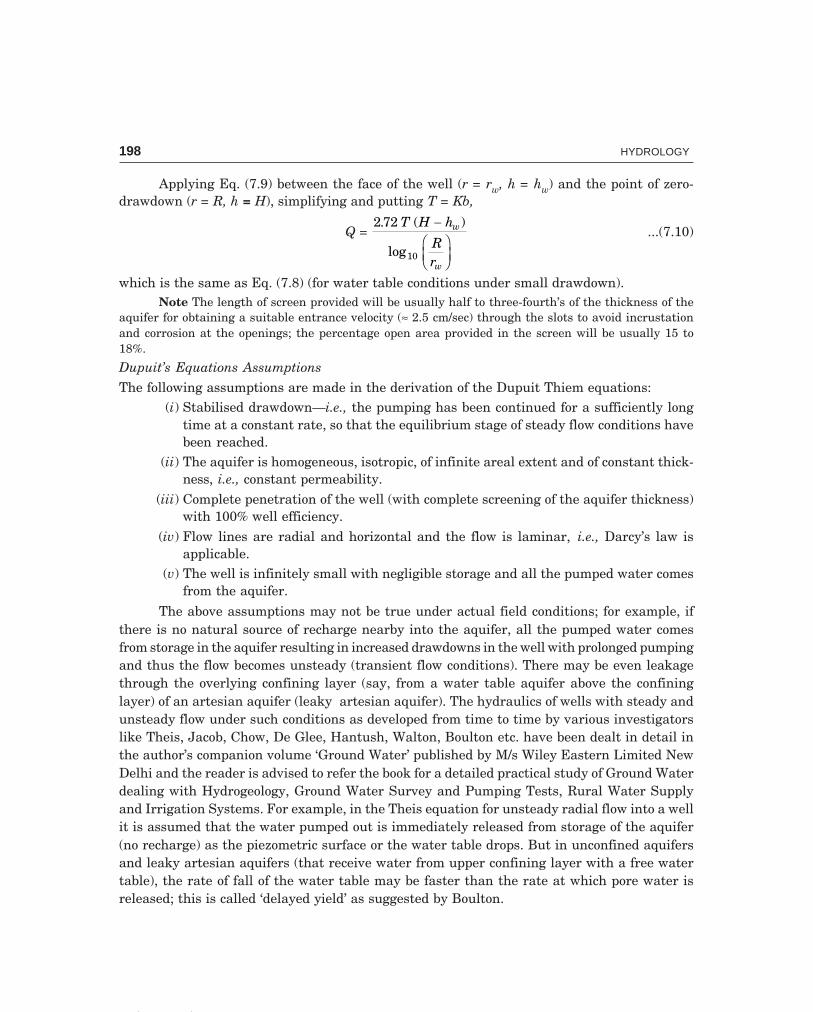
C-9\N-HYDRO\HYD7-1.PM5 198
198 HYDROLOGY
Applying Eq. (7.9) between the face of the well (r = rw, h = hw) and the point of zero-drawdown (r = R, h = H), simplifying and putting T = Kb,
Q = 2 72
10
. ( )
log
T H h
Rr
w
w
−FHG
IKJ
...(7.10)
which is the same as Eq. (7.8) (for water table conditions under small drawdown).Note The length of screen provided will be usually half to three-fourth’s of the thickness of the
aquifer for obtaining a suitable entrance velocity (≈ 2.5 cm/sec) through the slots to avoid incrustationand corrosion at the openings; the percentage open area provided in the screen will be usually 15 to18%.
Dupuit’s Equations Assumptions
The following assumptions are made in the derivation of the Dupuit Thiem equations:(i) Stabilised drawdown—i.e., the pumping has been continued for a sufficiently long
time at a constant rate, so that the equilibrium stage of steady flow conditions havebeen reached.
(ii) The aquifer is homogeneous, isotropic, of infinite areal extent and of constant thick-ness, i.e., constant permeability.
(iii) Complete penetration of the well (with complete screening of the aquifer thickness)with 100% well efficiency.
(iv) Flow lines are radial and horizontal and the flow is laminar, i.e., Darcy’s law isapplicable.
(v) The well is infinitely small with negligible storage and all the pumped water comesfrom the aquifer.
The above assumptions may not be true under actual field conditions; for example, ifthere is no natural source of recharge nearby into the aquifer, all the pumped water comesfrom storage in the aquifer resulting in increased drawdowns in the well with prolonged pumpingand thus the flow becomes unsteady (transient flow conditions). There may be even leakagethrough the overlying confining layer (say, from a water table aquifer above the confininglayer) of an artesian aquifer (leaky artesian aquifer). The hydraulics of wells with steady andunsteady flow under such conditions as developed from time to time by various investigatorslike Theis, Jacob, Chow, De Glee, Hantush, Walton, Boulton etc. have been dealt in detail inthe author’s companion volume ‘Ground Water’ published by M/s Wiley Eastern Limited NewDelhi and the reader is advised to refer the book for a detailed practical study of Ground Waterdealing with Hydrogeology, Ground Water Survey and Pumping Tests, Rural Water Supplyand Irrigation Systems. For example, in the Theis equation for unsteady radial flow into a wellit is assumed that the water pumped out is immediately released from storage of the aquifer(no recharge) as the piezometric surface or the water table drops. But in unconfined aquifersand leaky artesian aquifers (that receive water from upper confining layer with a free watertable), the rate of fall of the water table may be faster than the rate at which pore water isreleased; this is called ‘delayed yield’ as suggested by Boulton.

C-9\N-HYDRO\HYD7-1.PM5 199
GROUND WATER 199
7.6 SPECIFIC CAPACITY
The specific capacity QSw
of a well is the discharge per unit drawdown in the well and is
usually expressed as lpm/m. The specific capacity is a measure of the effectiveness of the well;it decreases with the increase in the pumping rate (Q) and prolonged pumping (time, t).
In Eq. (7.8) by putting rw = 15 cm, R = 300 m, H–hw = Sw, the specific capacity
QSw
≈ T12.
, in consistent units ...(7.11)
Example 7.3 A 20-cm well penetrates 30 m below static water level (GWT). After a long periodof pumping at a rate of 1800 lpm, the drawdowns in the observation wells at 12 m and 36 mfrom the pumped well are 1.2 m and 0.5 m, respectively.
Determine: (i) the transmissibility of the aquifer.(ii) the drawdown in the pumped well assuming R = 300 m.
(iii) the specific capacity of the well.
Solution Dupuit’s Eq. (7.7): Q = π K h h
r r( )
. log /22
12
10 2 12 303−
h2 = H – s2 = 30 – 0.5 = 29.5 m; h1 = H – s1 = 30 – 1.2 = 28.8 m
1.80060
= πK( . . )
. log /29 5 28 8
2 303 36 12
2 2
10
−
∴ K = 2.62 × 10⁻⁴ m/sec or 22.7 m/day(i) Transmissibility T = KH = (2.62 × 10⁻⁴) 30 = 78.6 × 10⁻⁴ m2/sec,
or = 22.7 × 30 = 681 m2/day
(ii) Eq. (7.8): Q = 2 72
10
. ( )log /
T H hR r
w
w
−
1800
60.
≡ 2 72 78.6 10
300 0 10
4
10
. ( )log / .
× − Sw
∴ drawdown in the well, Sw = 4.88 m(iii) The specific capacity of the well
= QSw
= 1800
60 4 88.
.× = 0.0062 (m3 sec–1/m)
or 372 Ipm/m
QSw
≈ T12.
= 78 6 10
12
4..× −
= 0.00655 (m2 sec–1/m)
or 393 lpm/mExample 7.4 A tube well taps an artesian aquifer. Find its yield in litres per hour for a drawdownof 3 m when the diameter of the well is 20 cm and the thickness of the aquifer is 30 m. Assumethe coefficient of permeability to be 35 m/day.
If the diameter of the well is doubled find the percentage increase in the yield, the otherconditions remaining the same. Assume the radius of influence as 300 m in both cases.

C-9\N-HYDRO\HYD7-1.PM5 200
200 HYDROLOGY
Solution Dupuit’s Eq. (7.10): Q = 2 72
10
. ( )log /
T H hR r
w
w
−
= 2 72 35 24 30 3
300 0 1010
. {( / ) }log ( / . )
× = 102.7 m3/hr
or = 102700 lph
The yield Q ∝ 1
log ( / )R rw...(7.12)
other things remaining same.If the yield is Q′ after doubling the diameter, i.e.,
rw′ = 0.10 × 2 = 0.20 m
QQ′ =
log /log /
R rR r
w
w
log 3000 10.
= 3.4771, log 3000 20.
= 3.1761
102 7.
′Q = 3 17613 4771..
∴ Q′ = 112.4 m3/hr
percentage increase in yield = ′ −Q QQ × 100 =
112 4 102 7102 4. .
.−
× 100 = 9.45%
Thus, by doubling the diameter the percentage in yield is only about 10%, which isuneconomical. Large diameter wells necessarily do not mean proportionately large yields. Thediameter of a tube well usually ranges from 20 to 30 cm so that the bowl assembly of a deepwell or a submersible pump can easily go inside with a minimum clearance.
Refer Appendix-D for Unsteady Groundwater Flow.
7.7 CAVITY WELLS
If a relatively thin impervious formation or a stiff clay layer is encountered at a shallow depthunderlain by a thick alluvial stratum, then it is an excellent location for a cavity well. A holeis drilled using the hand boring set and casing pipe is lowered to rest firmly on the stiff claylayer, Fig. 7.4. A hole of small cross-section area is drilled into the sand formation and isdeveloped into a big hollow cavity by pumping at a high rate or by operating a plunger givinga large yield. The depth of the cavity at the centre varies from 15-30 cm with 6-8 m radius ofthe cavity. The flow of water into the cavity is spherical and the yield is low. The failure of acavity well is usually due to caving of the clay roof. Since the depth is usually small, deep wellpumps are not necessary and thus the capital costs of construction, development and installa-tion of pumpset of a cavity well are low.
Yield of Cavity WellFor the unsteady flow condition, the pumping rate Q of a cavity well is given by
s = Q S
K t
Qkr
s
6 2π π+ ...(7.13)
where s = drawdown in the observation well at a distance r from the cavity wellQ = constant pumping rate

C-9\N-HYDRO\HYD7-1.PM5 201
GROUND WATER 201
Cavityy
Sand layers freefrom fine grainsSand layers freefrom fine grains
Extensively thickconfined aquiferExtensively thickconfined aquifer
Flow sphericalcritical velocity
surface
Flow sphericalcritical velocity
surface
Aquiclude (Imp.)Aquiclude (Imp.)
rere
hwhw
Stiff claylayer (Imp.)
Stiff claylayer (Imp.)
RRHH
o+Weathered
soil
Piezometric surface
Casing
Non-pumpingTop soil
QGS
rwrw
PWLPWL
Fig. 7.4 Flow into a cavity well
Ss = specific storage coefficient (i.e., for unit aquifer thickness)K = permeability of the aquifer t = time since pumping beganFor steady state flow condition, the well yield is given by
Q = 2
1πKy H h
r Rw
w
( )/−
− ...(7.14)
and the width of the cavity, Fig. 7.4
re = ( )2r y yw − ...(7.15)
where y = depth of cavity (at the centre)rw = radius of cavity R = radius of influence
Example 7.5 The following data are obtained from a cavity tube well:Discharge 30 lpsDrawdown 4 mPermeability of the aquifer 50 m/dayDepth of cavity 20 cmRadius of influence 150 m
Determine the radius and width of cavity.
Solution Well yield Q = 2
1
πKy H hrR
w
w
( )−
−
301000
= 2π × 50
24 60 600 20 4
1150
× ××
×
−
.rw

C-9\N-HYDRO\HYD7-1.PM5 202
202 HYDROLOGY
∴ Radius of cavity, rw = 135.5 m
Width of cavity, re = ( )2r y yw − = ( . . ) .2 4 5 0 2 0 2× − = 7.36 m
7.8 HYDRAULICS OF OPEN WELLS
Theis equation does not apply for shallow dug open wells since there is no instantaneous re-lease of water from the aquifer, most of the water being pumped only from storage inside thewell (Fig. 7.5).
GS
SWL
Recuperatedwater level
Recuperatedin time T
Depressedwater level
Impervious wellsteining
Flow into well
S2S2
S1S1
Fig. 7.5 Recuperation test in open wells
In alluvial soil, if the water is pumped at a high rate the depression head (static waterlevel–water level inside the well during pumping) will increase, which may cause excess gradi-ents resulting in loosening of sand particles (quick sand phenomenon). This limiting head iscalled ‘critical depression head’. The ‘safe working depression head’ is usually one-third of thecritical head and the yield under this head is called the maximum safe yield of the well.
Yield TestsThe following tests may be performed to get an idea of the probable yield of the well:
(a) Pumping test(b) Recuperation test(a) Pumping Test. In the pumping test, the water level in the well is depressed to an
amount equal to the safe working head for the sub-soil. Then the water level is kept constantby making the pumping rate equal to the percolation into the well. The quantity of waterpumped in a known time gives an idea of the probable yield of the well of the given diameter.The test may be carried out in an existing open well.
In hard-rock areas,if D = diameter of the well
d = depth of water columnQ = pumping rate t = time required for emptying the well
then,Rate of seepage into the well

C-9\N-HYDRO\HYD7-1.PM5 203
GROUND WATER 203
= Volume of water pumped out Volume of water stored in the well
Time of pumping−
= Qt
Dd
t
− ×π 2
4 ...(7.16)
(b) Recuperation Test. In the recuperation test, the water level in the well is depressedby an amount less than the safe working head for the subsoil. The pumping is stopped and thewater level is allowed to rise or recuperate. The depth of recuperation in a known time is notedfrom which the yield of the well may be calculated as follows (Fig. 7.5).
Let the water level inside the well rise from s1 to s2 (measured below static water level,swl) in time T. If s is the head at any time t, from Darcy’s law
Q = KAiif a head s is lost in a length L of seepage path
Q = KA sL
Q = CAs
where the constant C = KL
and has dimensions of T–1.
If in a time dt, the water level rises by an amount dsQ dt = – A ds
the –ve sign indicates that the head decreases as the time increases.Putting Q = CAs
CAs dt = – A ds
C 0
Tdtz =
s
s dss1
2z −
∴ C = 2 303.
T log10
ss
1
2...(7.17)
Assuming the flow is entirely from the bottom (impervious steining of masonry), theyield of the well
Q = CAH ...(7.17a)where Q = safe yield of the well
A = area of cross section of the wellH = safe working depression headC = specific yield of the soilFrom Eq. (7.17a) Q = C when A = 1, H = 1, i.e., the specific yield of the soil is the
discharge per unit area under a unit depression head and has dimension of T–1 (1/time) andthe usual values are
C = 0.25 hr–1 for clayey soilC = 0.50 hr–1 for fine sandC = 1.00 hr–1 for coarse sand
The value of C is usually determined from a recuperation test, (Eq. (7.17)).Example 7.6 A well of size 7.70 × 4.65 m and depth 6.15 m in lateritic soil has its normal
water level 5.08 m below ground level (bgl). By pumping for 1 12 hours, the water level was

C-9\N-HYDRO\HYD7-1.PM5 204
204 HYDROLOGY
depressed to 5.93 m bgl and the pumping was stopped. The recuperation rates of the well dur-ing 4 hours after the pumping stopped are given below. The total volume of water pumped
during 1 12 hours of pumping was 32.22 m3. (no well steining is provided)
Recuperation rates
Time sincepumping stopped Water level bgl
(min) (m)
0 5.930
15 5.89030 5.875
45 5.85560 5.840
90 5.820120 5.780
180 5.715240 5.680
Determine(i) Rate of seepage into the well during pumping.
(ii) Specific yield of the soil and specific capacity of the well.(iii) Yield of the well under a safe working depression head of 0.85 m.
(iv) The area of crop that can be irrigated under the well (assume a peak consumptive useof 4 mm and irrigation efficiency of 75%).
(v) Diameter of the well in such a soil to get an yield of 3000 lph under a safe workingdepression head of 0.8 m.
Solution (i) Seepage into the well—from pumping data:Volume of water pumped out = 32.22 m3
Volume of water stored in the well (that was pumped out)= (7.70 × 4.65) (5.93 – 5.08) = 30.5 m3
Rate of seepage into the well
= 32.22 30.5
1.5−
= 1.15 m3/hr
(ii) Specific yield of the soil
C = 2 303.
T log10
ss
1
2 =
2 3034
. log10
5 93 5 085 68 5 08. .. .
−−
= 0.09 hr–1 (or m3/hr per m drawdown)Specific capacity of the well is its yield per unit drawdown
Q = CAH

C-9\N-HYDRO\HYD7-1.PM5 205
GROUND WATER 205
∴ Specific capacity = Q/H = CA = 0.09 (7.70 × 4.65) = 3.58 m3 hr–1/m (or m2/hr)
(iii) Safe yield of the well Q = CAH = 0.09 (7.70 × 4.65) 0.85 = 3.04 m3/hr
which is more than twice the seepage into the well during pumping.(iv) Area of crop that can be irrigated under the well:Data to draw the curve s1/s2 vs. t (s1 = total drawdown, s2 = residual drawdown): SWL =
5.08 m, s1 = 5.93 – 5.08 = 0.85 m
Time since Water level Residual drawdownpumping stopped bgl s2 = wL – SWL Ratio (s1/s2)
t (min) (m) (m)
0 5.930 0.850 (= s1) 1.00
15 5.890 0.810 1.05
30 5.875 0.795 1.07
45 5.855 0.775 1.09
60 5.840 0.760 1.11
90 5.820 0.740 1.15
120 5.780 0.700 1.21
180 5.715 0.635 1.33
240 5.680 0.600 1.41
From the plot of ‘s1/s2 vs. time’ on a semi-log paper (Fig. 7.6), it is seen that s1/s2 = 9.5after 24 hours of recovery (by extending the straight line plot), and the residual drawdown
after 24 hours, s24 = 0 859 5..
≈ 0.09 m; hence the depth of recuperation per day = 0.85 – 0.09 = 0.76
m and the volume of water available per day ≈ (7.70 × 4.65) ≈ 27.2 m3. With an average peakconsumptive use of 4 mm for the type of crops grown and irrigation efficiency of 75%, the areaof crop (Acrop) that can be irrigated under one well in lateritic soils is
41000 0 75× .
× Acrop = 27.2
∴ Acrop = 5100 m2 or 0.5 ha(v) Diameter of the well to yield 3000 lph:
Q = CAH
30001000
= 0.09 × π × D2
4 × 0.8
∴ D = 7.3 m, which is too bigIt may be noted that it is not advisable to go deeper in these areas otherwise salt water
instrusion takes place.
C-9\N-HYDRO\HYD7-1.PM5 206
206 HYDROLOGY
Well dug in lateriticsoil near Mangalore
L B D= 7.70 4.65 6.15 m
´ ´´ ´
(KREC)
Semi-log paper
Extrapolated
Observeddata
109
8
7
6
5
4
3
2
1.5
S
S1
2= 9.5
10 2 4 6 8 10 12 14 16 18 20 22 24
Recuperation time t (hr)
Rat
ioS S
1 2
Fig. 7.6 Plot of recuperation test data (Example 7.6)
7.9 CONSTRUCTION OF OPEN WELLS
In alluvial soil, where an impervious vertical steining is provided to support the soil, percola-tion into the well is entirely from the bottom and depends on the area of cross-section of thewell. Bigger diameter wells are recommended in such soil to give larger yields. In case of wellsin rocky substrata with fissures and cracks, the lower portion of the steining may be providedwith alternate bands of masonry laid dry (i.e., without cement mortar) (Fig. 7.7), and thepercolation into the well is mostly from the sides through fissures and cracks in the weatheredrock. In such wells, higher yields are obtained by going deeper, as long as the weathering andfractures are evident rather than making the wells wider or larger diameter. Larger diameterwells also involve large volume of excavation in rocks and the mounds of excavated rock depos-ited on the ground surface occupy considerable area of cultivable land. Sometimes, it is pro-posed to widen when it is felt that such widening will, include some well-defined fissures andfractures.
Some of the existing wells may be revitalised by deepening by blasting; vertical boresmay be drilled at the bottom of the well when it is felt it will tap some layer under pressure,i.e., a dug-cum-borewell (Fig. 7.8), with a centrifugal pump kept at the bottom of the open welland the suction pipe lowered inside the bore, thus reducing the suction lift and saving the costsinvolved in deep well turbine pump or submersible pump installations in drilled deep wellsfrom the ground surface. Lateral bores horizontal or inclined, may be drilled in the direction ofcertain well-defined fractures yielding water.

C-9\N-HYDRO\HYD7-1.PM5 207
GROUND WATER 207
GS
DD
dd
NPWL
PWL
RCC Curb
Weep holes
Vertical tie rods
Flat iron rings
Foot valve
Flow into well
Centrifugalpump & motor
Aquifer
Q
Fig. 7.7 Open well construction
Very hard rock
Coarse sandCoarse sand
Hard rockBore drilled
WaterWeathered
rockDug well
Well-steining
Top soil
GS
Fig. 7.8 Dug-cum-borewell
7.10 SPACING OF WELLS
Pumping wells should be spaced far apart so that their cones of depression will not overlapover each other resulting in the reduction of their yields and/or increased drawdowns (Fig.7.9),i.e., to avoid ‘well interference’, the wells should be spaced beyond their radii of influence. Thisis roughly estimated to be around 600–1000 m in alluvial area and around 100–200 m in hardrock areas.
An open dug well should be located beyond the cone of depression of the tubewell; other-wise when the tubewell is pumping, it will dewater the open well. The open well can get wateronly when the tubewell pumping is stopped and fast recuperation takes place.

C-9\N-HYDRO\HYD7-1.PM5 208
208 HYDROLOGY
Wells closely spaced inhomogeneous
aquifer
Wells closely spaced inhomogeneous
aquifer
Spacing ofwells
Spacing ofwells
Interferenceof cones
Interferenceof cones
Cones of drawdownCones of drawdownPWLPWL
Increased drawdown dueto interference
Increased drawdown dueto interference
dwdwdwdwdwdwdwdw
PWLPWL
GS PWQ
PWQ
SWL (NPWL)SWL (NPWL)
Dug wellbecomes dry
dw: Dewatered zonePW: Pumped wells
Fig. 7.9 Well interference
��������
I Choose the correct statement/s in the following:
1 The underground formations, which serve as good aquifers are in the order:
(i) consolidated formations of clays and shales
(ii) rock with no signs of weathering or fractures
(iii) rock with fissures and cracks (iv) cavernous lime stones
(v) sand stones (vi) vescicular basalts
(vii) unconsolidated gravels, sands and alluvium
2 The soil properties characteristic of good water yield are:
(i) porosity (ii) permeability
(iii) specific yield (iv) storage coefficient
(v) transmissibility (vi) uniformity coefficient > 3
(vii) uniformity coefficient < 2 (viii) effective size > 0.1 mm
(ix) Reynolds number > 10 (x) specific capacity of the well > 30 lpm/m
(xi) all the above characteristics (1-except i, ii, 2 ii, iii, iv, v, viii, x)
II Match the items in ‘A’ with the items in ‘B’:
A B(i) Ground water flow (a) Recuperation test
(ii) Unconsolidated alluvium (b) Bore at the bottom of open well
(iii) Aquiclude (c) Lateral or vertical bores
(iv) Specific yield (Sy) (d) Well spacing
(v) Confined aquifer (e) n – Sr
(vi) Storage coefficient (f) Artesian
(vii) Transmissibility (T) (g) f(Kw, Es)

C-9\N-HYDRO\HYD7-1.PM5 209
GROUND WATER 209
(viii) Rate of ground water flow (Q) (h) KH or Kb
(ix) Reynolds number (Re) (i) T iW
(x) Dupuit’s equation (j) ρvd/µ
(xi) Specific capacity (k)Qsw
T≈12.
(xii) Open well (l) Stabilised drawdown
(xiii) Well revitalisation (m) Clay
(xiv) Dug-cum-borewell (n) Aquifer
(xv) Well interference (o) Darcy’s law
III Say ‘true’ or ‘false’; if false, give the correct statement:
(i) The transmissibility of a confined aquifer depends upon the depth of the water table whilethat of the water table aquifer does not.
(ii) The available yield of a tube well can be doubled by doubling the diameter.
(iii) The specific yield of an aquifer may be more than its porosity.
(iv) Storage coefficient is the same as specific yield for a water table aquifer.
(v) Flow in a medium sand aquifer is entirely laminar.
(vi) Plants usually extract water from the capillary zone (the intermediate belt or vadose zone).
(false: i, ii, iii)
�������
1 (a) Define ‘transmissibility’ and ‘storage coefficient’ of an aquifer.
(b) Calculate the discharge from a tubewell of 20-cm diameter penetrating fully into a confinedaquifer of 20-m thick and having a permeability of 40 m/day. The drawdown in the well is3 m and zero drawdown at 300 m from the well.
If the diameter of the well is doubled, find the percentage increase in the yield, the otherconditions remaining the same.
State the assumptions in the formula you use. (1303.7 lpm)
2 A tubwell penetrates fully an unconfined aquifer. Calculate the discharge from the well in lpmfrom the following data:
Diameter of the well 30 cm
Drawdown in the well 3 m
Effective length of the strainer under the abovedrawdown 10 m
Coefficient of permeability of the aquifer 40 m/day
Radius of zero drawdown 300 m
3 A 20-cm well penetrates 25 m below the static water table. After 24 hours of pumping out at therate of 800 lpm, the water level in a test well at 80 m from the pumping well is lowered by 0.53m and in a test well 20 m away 2.11 m. Find the coefficient of transmissibility of the aquifer.
4 (a) What is the nature of ground water flow? State the law governing the flow with limitations,if any.
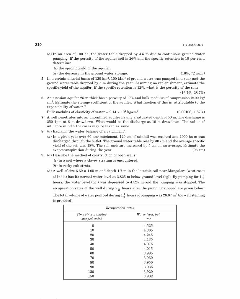
C-9\N-HYDRO\HYD7-1.PM5 210
210 HYDROLOGY
(b) In an area of 100 ha, the water table dropped by 4.5 m due to continuous ground waterpumping. If the porosity of the aquifer soil is 26% and the specific retention is 10 per cent,determine:(i) the specific yield of the aquifer.
(ii) the decrease in the ground water storage. (16%, 72 ham)5 In a certain alluvial basin of 120 km2, 100 Mm3 of ground water was pumped in a year and the
ground water table dropped by 5 m during the year. Assuming no replenishment, estimate thespecific yield of the aquifer. If the specific retention is 12%, what is the porosity of the soil?
(16.7%, 28.7%)6 An artesian aquifer 25-m thick has a porosity of 17% and bulk modulus of compression 2400 kg/
cm2. Estimate the storage coefficient of the aquifer. What fraction of this is attributable to theexpansibility of water ?Bulk modulus of elasticity of water = 2.14 × 10⁴ kg/cm2. (0.00106, 1.87%)
7 A well penetrates into an unconfined aquifer having a saturated depth of 50 m. The discharge is250 1pm at 8 m drawdown. What would be the discharge at 10 m drawdown. The radius ofinfluence in both the cases may be taken as same.
8 (a) Explain: ‘the water balance of a catchment’.(b) In a given year over 60 km2 catchment, 120 cm of rainfall was received and 1000 ha-m was
discharged through the outlet. The ground water table rose by 30 cm and the average specificyield of the soil was 18%. The soil moisture increased by 5 cm on an average. Estimate theevapotranspiration during the year. (93 cm)
9 (a) Describe the method of construction of open wells(i) in a soil where a clayey stratum is encountered.
(ii) in rocky sub-strata.(b) A well of size 6.60 × 4.05 m and depth 4.7 m in the lateritic soil near Mangalore (west coast
of India) has its normal water level at 3.825 m below ground level (bgl). By pumping for 1 12
hours, the water level (bgl) was depressed to 4.525 m and the pumping was stopped. The
recuperation rates of the well during 2 12 hours after the pumping stopped are given below.
The total volume of water pumped during 1 12 hours of pumping was 28.87 m3 (no well steining
is provided)
Recuperation rates
Time since pumping Water level, bglstopped (min) (m)
0 4.52510 4.36520 4.24530 4.13540 4.07550 4.01560 3.98570 3.96080 3.95090 3.935
120 3.920150 3.902

C-9\N-HYDRO\HYD7-1.PM5 211
GROUND WATER 211
Determine
(i) Rate of seepage into the well during pumping
(ii) Specific yield of the soil and specific capacity of the well
(iii) Yield of the well under a safe working depression head of 0.7 m
(iv) The area of crop that can be irrigated under the well, assuming a peak consumptive use of4 mm and irrigation efficiency of 75%.
(v) Diameter of the well in such a soil to get an yield of 3000 lph under a safe working depressionhead of 0.7 m (note that it is not advisable to go deeper in these areas lest salt water intru-sion may not take place).
10 In a recuperation test, the static water level in an open well was depressed by pumping by 3 mand it recuperated 1.5 m in 1 hour. If the diameter of the well is 3 m and the safe workingdepression head is 2.4 m, find the average yield of the well in lpm. What area of crop can comeunder this well assuming a peak consumptive use of 5 mm and irrigation efficiency of 75%?
11 Determine the diameter of an open well in coarse sand to give an average yield of 200 lpm undera safe working depression head of 2.5 m (Hint: for coarse sand C ≈ 1 hr–1).
12 Distinguish between:
(i) Specific capacity of a well and specific yield of an aquifer
(ii) Aquifer and acuiclude
(iii) Open wells and tube wells
(iv) Water table and artesian aquifers
(v) Drainage divide and ground water divide
13 Write short notes on:
(i) Well development (ii) Well spacing
(iii) Radius of influence (iv) Validity of Darcy’s law
(v) Dug-cum-borewell (vi) Well revitalisation
(vii) Well interference (viii) Recuperation test for open well

8.1 SIZE OF FLOODS
A flood is an unusual high stage of a river due to runoff from rainfall and/or melting of snow inquantities too great to be confined in the normal water surface elevations of the river or stream,as the result of unusual meteorological combination.
The maximum flood that any structure can safely pass is called the ‘design flood’ and isselected after consideration of economic and hydrologic factors. The design flood is related tothe project feature; for example, the spillway design flood may be much higher than the floodcontrol reservoir design flood or the design flood adopted for the temporary coffer dams. Adesign flood may be arrived by considering the cost of constructing the structure to provideflood control and the flood control benefits arising directly by prevention of damage to structuresdownstream, disruption communication, loss of life and property, damage to crops and under-utilisation of land and indirectly, the money saved under insurance and workmen’scompensation laws, higher yields from intensive cultivation of protected lands and eliminationof losses arising from interruption of business, reduction in diseases resulting from inundationof flood waters. The direct benefits are called tangible benefits and the indirect benefits arecalled intangible benefits. The design flood is usually selected after making a cost-benefit analysisand exercising engineering judgement.
When the structure is designed for a flood less than the maximum probable, there existsa certain amount of flood risk to the structure, nor is it economical to design for 100% floodprotection. Protection against the highest rare floods is uneconomical because of the largeinvestment and infrequent flood occurrence.
In the design flood estimates, reference is usually made to three classes:(a) Standard Project Flood (SPF). This is the estimate of the flood likely to occur from
the most severe combination of the meteorological and hydrological conditions, which are rea-sonably characteristic of the drainage basin being considered, but excluding extremely rarecombination.
(b) Maximum Probable Flood (MPF). This differs from the SPF in that it includes theextremely rare and catastrophic floods and is usually confined to spillway design of very highdams. The SPF is usually around 80% of the MPF for the basin.
(c) Probable Maximum Precipitation (PMP). From the observations of air moisture fromthe maximum due-point and temperature recorded and air-inflow (from the wind speed andbarometric pressure recorded), the moisture inflow index in the storm is determined. The bestknown upward adjustment to be applied to the historical and hypothetical major storms is the
Chapter 8
FLOODS-ESTIMATION AND CONTROL
212

C-9\N-HYDRO\HYD8-1.PM5 213
FLOODS-ESTIMATION AND CONTROL 213
maximisation with respect to moisture charge. The adjusted storm rainfall is assumed to bearthe same ratio to the observed storm rainfall, as the maximum moisture charge over the basinto the moisture charge of the observed storm. From the critical combinations of storms, andmoisture adjustment the PMP is derived which, after minimising losses, when applied on thedesign unit hydrograph for the basin, will produce the MPF. Occasionally when enough stormdata for the given basin is not available, PMP can be estimated by adopting a severe stormover neighbouring catchment (which is meteorologically homogeneous) and transposing it tothe catchment under consideration.
(d) Design Flood—It is the flood adopted for the design of hydraulic structures likespillways, bridge openings, flood banks, etc. It may be the MPF or SPF or a flood of any desiredrecurrence interval depending upon the degree of flood protection to be offered and cost eco-nomics of construction of structures to the desired flood stage; the design flood is usually se-lected after making a cost-benefit analysis, i.e., the ratio of benefit to cost may be desired to bethe maximum.
8.2 ESTIMATION OF PEAK FLOOD
The maximum flood discharge (peak flood) in a river may be determined by the followingmethods:
(i) Physical indications of past floods—flood marks and local enquiry(ii) Empirical formulae and curves (iii) Concentration time method(iv) Overland flow hydrograph (v) Rational method(vi) Unit hydrograph (vii) Flood frequency studiesThe above methods are discussed below:(i) Observations at nearby structure. By noting the flood marks (and by local enquiry),
depths, affluxes (heading up of water near bridge openings, or similar obstructions to flow)and other items actually at an existing bridge, on anecut (weir) in the vicinity, the maximumflood discharge may be estimated. The flood marks are connected by levelling, the profile isplotted and HFL marked on it, and the cross sectional area is determined. The surface fall atHFL is calculated from the difference in HFL at known distance apart. It may be checked withthe bed slope; there should not be much disparity between the two. By assuming a suitablevalue of Manning’s n for the nature (roughness) of bed and sides of the river, the velocity maybe determined by Manning’s or Chezy’s formula and the flood discharge estimated, seeexample 6.4.
(ii) Empirical Flood Formulae
1. Dickens formula for moderate size basins of north and central IndiaQ = CA3/4 ...(8.1)
the coefficient C = 11–14, where the aar is 60–120 cm= 14–19 in Madhya Pradesh= 32 in western Ghats
up to 35, maximum value2. Ryves formula derived from a study of rivers in south India
A = CA2/3 ...(8.2)

C-9\N-HYDRO\HYD8-1.PM5 214
214 HYDROLOGY
Coefficient C = 6.8 within 80 km of coast= 8.3 for areas between 80 and 2400 km from the coast= 10.0 for limited area near the hills
up to 40, actual observed values3. Inglis formula for fan-shaped catchments of Bombay state (Maharashtra)
Q = 124
10 4
A
A + ....(8.3)
4. Myers formula Q = 175 A ...(8.4)
5. Ali Nawab Jang Bahadur formula for the old Hyderabad state
Q = CA(0.993 – 1/14 log A) ...(8.5)
the coefficient C varies from 48 to 60
Maximum value of C = 85
6. Fuller’s formula (1914)
Q = CA0.8 (1 + 0.8 log TT)(1 + 2.67 A–0.3) ...(8.6)
constants derived from the basins in USA 10 years data is required for sufficientreliability. The coefficient C varies from 0.026 to 2.77; T = recurrence interval inyears. Fuller was the first to suggest that frequency should be considered as a factorin estimating floods.
7. Greager’s formula for USA
Q = C( . ) ( ) .0 386 0.894 0.386 0 048
A A −...(8.7)
the coefficient C ≈ 130 (140.5 for areas most favourable to large floods)
8. Burkli Ziegler formula for USA
Q = 412 A3/4 ...(8.8)
In all the above formula, Q is the peak flood in cumec and A is the area of the drainagebasin in km2.
(iii) Envelope Curves. Areas having similar topographical features and climatic condi-tions are grouped together. All available data regarding discharges and flood formulae arecompiled along with their respective catchment areas. Peak flood discharges are then plottedagainst the drainage areas and a curve is drawn to cover or envelope the highest plotted points.Envelope curves are generally used for comparison only and the design floods got by othermethods, should be higher than those obtained from envelope curves. For Indian rivers, envel-oping curves from observed floods have been developed by Kanwar Sain and Karpov, Fig. 8.1 (a).
(iv) Concentration Time Method. The concentration time method of estimating the peakdischarge consists of two steps:
(i) Determination of the concentration time, etc.
(ii) Selection of the period of maximum net rainfall for the concentration time duration.This method can be used for design storms or in conjunction with intensity-duration-frequency curves.

C-9\N-HYDRO\HYD8-1.PM5 215
FLOODS-ESTIMATION AND CONTROL 215
Log-log paperLog-log paper
10080
60
40
30
20
108
6
4
3
2
11 2 3 4 5 6 8 10 20 30 40 60 80100 200 300 5007001000
1
10
100100010010M
axim
umflo
oddi
scha
rge
(100
0cu
mec
)
Catchment area (1000 km )2
Rivers in northand central India
Rivers in northand central India
Rivers in south India
Rivers in south India
1
Fig. 8.1(a) Enveloping curves of Kanwar Sain and Karpov
Example 8.1 Determine the peak discharge at the concentration point for a basin of 80 hec-tares having a time of concentration of 30 minutes due to a 5-cm flash storm, if the duration ofthe storm is (i) 60 min, (ii) 30 min, and (iii) 15 min. Assume a φ-index of 2.5 cm/hr for the entirebasin. When the storm duration is 15 minutes, only drainage from 60% of the area of the basinreaches the concentration point.Solution
Q = (i – φ) A, where i = intensity of rainfall (cm/hr)(i) Q = (5 – 2.5) 80 = 200 ha-cm = 200 × 0.028 = 5.6 cumec
(ii) Q = ( 530 × 60 – 2.5) 80 = 600 ha-cm = 600 × 0.028 = 16.8 cumec
(iii) Q = ( 515 × 60 – 2.5) (0.60 × 80) = 840 ha-cm = 840 × 0.028 = 23.52 cumec
It is seen from (i) and (ii) that the peak discharge at the concentration point is maxi-mum when the duration of storm is equal to the time of concentration, (iii) gives the highestflood, since only 60% of the area drains, the concentration time becomes less and the intensityof rainfall is very high during this time.
(v) Rational Method. The rational method is based on the application of the formulaQ = CiA ...(8.9)
where C is a coefficient depending on the runoff qualities of the catchment called the runoffcoefficient (0.2 to 0.8). The intensity of rainfall i is equal to the design intensity or criticalintensity of rainfall ic corresponding to the time of concentration tc for the catchment for agiven recurrence interval T; the design intensity of rainfall i (= ic) can be found from theintensity-duration-frequency curves, for the catchment corresponding to tc and T. If theintensity-duration-frequency curves, are not available for the catchment and a maximumprecipitation of P cm occurs during a storm period of tR hours, then the design intensity i (= ic)can be obtained from the equation
C-9\N-HYDRO\HYD8-1.PM5 216
216 HYDROLOGY
ic = Pt
ttR
R
c
++
FHG
IKJ
11
...(8.10)
when the time of concentration, tc is not known, ic ≈ P/tR.The values of the runoff coefficient C are given in Table 8.1 and serve as a rough guide.
Table 8.1 Value of the runoff coefficient C
Type of terrain Value of C
Flat residential areas 0.4
Moderately steep residential area 0.6
Built up areas—impervious 0.8
Rolling lands and clay-loam soils 0.5
Hilly areas, forests, clay and loamy soils 0.5
Flat cultivated lands and sandy soils 0.2
Example 8.2 For an area of 20 hectares of 20 minutes concentration time, determine the peakdischarge corresponding to a storm of 25-year recurrence interval. Assume a runoff coefficientof 0.6. From intensity-duration-frequency curves for the area, for T = 25-yr, t = 20 min, i = 12cm/hr.Solution For t = tc = 20 min, T = 25-yr, i = ic = 12 cm/hr
Q = CiA = 0.6 × 12 × 20 = 144 ha-cm/hr = 144 × 0.028 = 4 cumec
Note 1 ha-cm/hr = 1
36 cumec = 0.028 cumec
Example 8.3 Determine the design flood discharge (allowing an increase of one-third) for abridge site with the following data:
Catchment area = 2 × 10⁵ ha
Duration of storm = 8 hoursStorm precipitation = 3 cm
Time of concentration = 2 hrGauged discharge for a past flood with average maximum daily rainfall of 18 cm was
3400 cumec.
Solution From the past flood,
Runoff coefficient, C = Actual discharge
Theoretical discharge
= 3400
2 10 1018
1001
24 60 605 4× × × ×
× ×
= 0.815
Design or critical intensity of rainfall
i = ic = Pt
ttR
R
c
++
FHG
IKJ
11
= 38
8 12 1
++
FHG
IKJ = 1.125 cm/hr
Q = CiA = 0.815 × 1.125 × (2 × 105) = 1.83 × 10⁵ ha-cm/hror, (1.83 × 10⁵) 0.028 = 5130 cumec
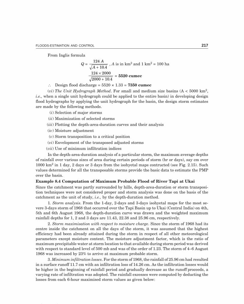
C-9\N-HYDRO\HYD8-1.PM5 217
FLOODS-ESTIMATION AND CONTROL 217
From Inglis formula
Q = 124
10 4
A
A + . , A is in km2 and 1 km2 = 100 ha
124 2000
2000 10 4
×+ .
= 5520 cumec
∴ Design flood discharge = 5520 × 1.33 = 7350 cumec(vi) The Unit Hydrograph Method. For small and medium size basins (A < 5000 km2,
i.e., when a single unit hydrograph could be applied to the entire basin) in developing designflood hydrographs by applying the unit hydrograph for the basin, the design storm estimatesare made by the following methods.
(i) Selection of major storms(ii) Maximization of selected storms
(iii) Plotting the depth-area-duration curves and their analysis(iv) Moisture adjustment(v) Storm transposition to a critical position
(vi) Envelopment of the transposed adjusted storms(vii) Use of minimum infiltration indicesIn the depth-area-duration analysis of a particular storm, the maximum average depths
of rainfall over various sizes of area during certain periods of storm (hr or days), say cm over1000 km2 in 1 day, 2 days or 3 days from the isohyetal maps contructed (see Fig. 2.15). Suchvalues determined for all the transposable storms provide the basic data to estimate the PMPover the basin.Example 8.4 Computation of Maximum Probable Flood of River Tapi at UkaiSince the catchment was partly surrounded by hills, depth-area-duration or storm transposi-tion techniques were not considered proper and storm analysis was done on the basis of thecatchment as the unit of study, i.e., by the depth-duration method.
1. Storm analysis. From the 1-day, 2-days and 3-days isohyetal maps for the most se-vere 3-days storm of 1968 that occurred over the Tapi Basin up to Ukai (Central India) on 4th,5th and 6th August 1968, the depth-duration curve was drawn and the weighted maximumrainfall depths for 1, 2 and 3 days are 11.43, 22.38 and 25.96 cm, respectively.
2. Storm maximisation with respect to moisture charge. Since the storm of 1968 had itscentre inside the catchment on all the days of the storm, it was assumed that the highestefficiency had been already attained during the storm in respect of all other meteorologicalparameters except moisture content. The moisture adjustment factor, which is the ratio ofmaximum precipitable water at storm location to that available during storm period was derivedwith respect to standard level of 500 mb and was of the order of 1.23. The storm of 4–6 August1968 was increased by 23% to arrive at maximum probable storm.
3. Minimum infiltration losses. For the storm of 1968, the rainfall of 25.96 cm had resultedin a surface runoff 11.7 cm with an infiltration loss of 14.26 cm. As the infiltration losses wouldbe higher in the beginning of rainfall period and gradually decrease as the runoff proceeds, avarying rate of infiltration was adopted. The rainfall excesses were computed by deducting thelosses from each 6-hour maximised storm values as given below:
C-9\N-HYDRO\HYD8-1.PM5 218
218 HYDROLOGY
Rainfall during Infiltration rate Infiltration loss in Rainfall6-hr interval (cm/hr) 6-hr interval excess
(cm) (cm) (cm)
10.5 0.25 1.5 9.0
6.0 0.25 1.5 4.5
4.4 0.24 1.44 2.96
2.7 0.24 1.44 1.26
1.5 0.23 1.38 0.12
1.0 0.23 1.38 –
0.8 0.23 1.38 –
0.6 0.23 1.38 –
1.3 0.20 1.20 0.10
1.1 0.20 1.20 –
1.0 0.20 1.20 –
0.9 0.20 1.20 –
31.8 17.94
Total loss = 31.80 – 17.94 = 13.86 cm
4. Maximum probable flood hydrograph. The 6-hour rainfall excesses were rearrangedin a sequence so as to produce the most severe flood peak and then applied to the ordinates ofthe 6-hour design unit hydrograph derived from the 1968 flood hydrograph at Kakrapar weirat Ukai with a lag of 6 hours successively and the ordinates of the surface runoff hydrograph ofthe maximum probable flood arrived at. The constant base flow of 2400 cumec was then addedto arrive at the final ordinates of the flood hydrograph of maximum probable flood (MPF). Thepeak of this hydrograph is 59800 cumec, Table 8.2, and is shown in Fig. 8.1. The highest peakattained during 1876-1968 (93 years) was 42500 cumec in August 1968 and the second highestwas 37300 cumec in September 1959. The MPF recommended by CWPC, India for the designof Ukai dam was almost the same as 59800 cumec while the SPF recommended was around48200 cumec. The design flood adopted was 49500 cumec.
5. Limitation. Unit hydrograph is generally applicable for catchments of less than 5000km2 since according to the theory, storm distribution over the area is assumed to be fairlyeven. The catchment of Tapi river up to Ukai dam is nearly 62000 km2 which is considerablygreater than the limit for unit hydrograph application. In such cases, the correct method wouldbe to subdivide the whole catchment into a number of sub-basins, and separately carry outunit hydrograph application for these sub-basins, and thereafter to arrive at the maximumflood for the catchment by routing the flood through the various river reaches. But this methodnaturally requires extensive gauge and discharge data for the individual sub-basins and at thelowest side, as also intermediate cross section of the river channel for the whole reach in orderto enable routing of the floods derived for the sub-basins. For Tapi, however, such extensivedata was not available and the catchment could not be sub-divided into sub-basins; the wholecatchment up to Ukai dam has been treated as a single unit.

C-9\N-HYDRO\HYD8-1.PM5 219
FLOODS-ESTIMATION AND CONTROL 219T
able
8.2
Com
puta
tion
of
max
imu
m p
roba
ble
floo
d of
Riv
er T
api
at U
kai,
A =
620
00 k
m2 .
(E
xam
ple
8.4)
Tim
e6-
hr
UG
OR
ain
fall
exc
esse
sD
RO
BF
OT
RO
(hr)
(cu
mec
)0.
121.
264.
59.
02.
96su
b-to
tal
(cu
mec
)(c
um
ec)
(cu
mec
)
00
00
2400
2400
627
931
031
024
0027
10
1293
510
535
010
7524
0034
75
1819
4022
011
812
560
3534
2400
5934
2425
0028
324
442
0025
120
9739
2400
1213
9
3030
0034
031
587
0085
1082
521
690
2400
2409
0
3633
4037
837
811
240
1750
027
6435
600
2400
3800
0
4232
2036
442
013
500
2252
057
5045
774
2400
4817
4
4829
4033
340
515
000
2700
074
0053
078
2400
5547
8
5426
6030
137
014
600
3060
088
7057
401
2400
5980
1←
pea
k
6020
5023
333
513
200
2900
098
9054
708
2400
5710
8
6612
8014
525
811
960
2648
095
3049
653
2400
5205
3
7296
310
916
192
0023
980
8700
4311
324
0045
513
7877
588
121
5730
1850
078
7033
084
2400
3548
4
8465
174
9843
3011
500
6070
2262
324
0025
023 (C
ontd
...)
p. 2
20

C-9\N-HYDRO\HYD8-1.PM5 220
220 HYDROLOGY
9054
061
8234
9081
7037
9016
133
2400
1853
3
9641
847
6829
3069
8028
5013
293
2400
1569
3
102
329
3753
2430
5860
2290
1099
924
0013
399
108
267
3041
1880
4860
1930
9007
2400
1140
7
114
212
2434
1480
3770
1600
7120
2400
9520
120
156
1827
1200
2960
1240
5601
2400
8001
126
111
1320
950
2400
974
4468
2400
6868
132
8610
1469
819
1079
035
0824
0059
08
138
587
1149
714
0462
726
0424
0050
04
144
314
738
710
0046
218
9124
0042
91
150
00
426
177
432
913
6824
0037
68
156
014
052
225
491
624
0033
16
162
027
917
245
124
0028
51
168
092
9224
0024
92
174
00
2400
2403
C-9\N-HYDRO\HYD8-1.PM5 221
FLOODS-ESTIMATION AND CONTROL 221
65
60
55
50
45
40
35
30
65
25
20
15
10
5
0
.121.26
4.5 9.0 cm
2.96P -max probable
(Rearranged)net
30 hr30 hr66 66 66 66 66
hr
Rai
nfal
lin
tens
ityi,
(cm
/hr)
A = 62000 km2
Design flood = 49500 cumec (D.F.)
59800 cumec = MPF48200 = SPF CWPC
cumec
42500 = 1968 Floodcumec (maximum)
Flood hydrograph 36
32
28
24
20
16
12
8
4
Dis
char
geQ
(6-h
rU
G),
(100
cum
ec)
Flo
oddi
scha
rge
Q(1
000
cum
ec)
0
0 12 24 36 48 60 72 96 108 120 132 144 156 168 180174150
Constant base flow = 2400 cumecConstant base flow = 2400 cumec
Time t (hr)
6-hr design UG(Q- scale exaggerated)
MPFMPF
D.F.D.F.
19681968
Fig. 8.1 MPF of river Tapi at Ukai (Example 8.4)
8.4 FLOOD FREQUENCY STUDIES
When stream flow peaks are arranged in the descending order of magnitude they constitute astatistical array whose distribution can be expressed in terms of frequency of occurrence. Thereare two methods of compiling flood peak data—the annual floods and the partial durationseries. In the annual floods, only the highest flood in each year is used thus ignoring the nexthighest in any year, which sometimes may exceed many of the annual maximum. In the par-tial duration series, all floods above a selected minimum are taken for analysis, regardless ofthe time-interval, so that in some years there may be a number of floods above the basic stage,while in some other years there may not any such flood at all. The disadvantage of the partialduration series is that the data do not furnish a proper frequency (true distribution) series andso a reasonable statistical analysis cannot be made. But all the larger floods are used in thisanalysis, which is an advantage while in annual flood series some big floods are omitted be-cause they were not the highest floods in any year considered. Usually the basic stage is as-sumed sufficiently low so that as many peaks (4 or 5) as possible each year are above thisstage. The two series give very nearly the same recurrence interval for the larger floods, butthe partial series indicates higher floods for shorter recurrence intervals. For information aboutfloods of fairly frequent occurrence, as is required during the construction period of a largedam (say, 4-5 years), the partial series are the best, while for the spillway design flood the

C-9\N-HYDRO\HYD8-1.PM5 222
222 HYDROLOGY
annual series are preferable, since the flood should not be exceeded in the dam’s life time, say100 years.
Annual Flood Series The return period or recurrence interval (T) is the average numberof years during which a flood of given magnitude will be equalled or exceeded once and iscomputed by one of the following methods.
California method (1923):
T = nm
...(8.11)
Allen Hazen method (1930):
T = n
mn
m−=
−12
22 1
...(8.11 a)
Weilbul method (1939):
T = n
m+ 1
...(8.11 b)
where n = number of events, i.e., years of recordm = order or rank of the event (flood item) when the flood magnitudes (items) are ar-
ranged in the descending order (m = 1 for the highest flood, m = n for the lowestflood)
T = recurrence interval (T = n-yr for the highest flood, T = 1 yr for the lowest flood, byCalifornia method)
The probability of occurrence of a flood (having a recurrence interval T-yr) in any year,i.e., the probability of exceedance, is
P = 1T
...(8.12)
or the percent chance of its occurrence in any one year, i.e., frequency (F) is
F = 1T
× 100 ...(8.12 a)
and the probability that it will not occur in a given year, i.e., the probability of non-exceedance(P′), is
P′ = 1 – P ...(8.12 b)One interesting example of the application of statistics to a hydrologic problem (i.e.,
stochastic hydrology), is Gumbel’s theory of extreme values. The probability of an event ofmagnitude x not being equalled or exceeded (the probability of non-occurrence, P′), based onthe argument that the distribution of floods is unlimited (i.e., for large values of n, say n > 50),
P′ = e e y− −...(8.13)
and the probability of the event x being equalled or exceeded (i.e., probability of occurrence, P) is
P = 1 – P′ = 1 – e e y− −...(8.13 a)
where e = base of natural logarithmsy = a reduced variate given by
y = 1
0 78. σ (x – x + 0.45 σ), for n > 50 ...(8.14)
x = flood magnitude with the probability of occurrence, P
x = arithmetic mean of all the floods in the series

C-9\N-HYDRO\HYD8-1.PM5 223
FLOODS-ESTIMATION AND CONTROL 223
x = Σxn
, x2 = Σxn
2
σ = standard deviation of the flood series
= Σ ( )x x
n−−
2
1
= n
nx x
−−
12 2[ ( ) ] ...(8.15)
= Σ Σx x n
n
2 2
1−
−( ) /
...(8.15 a)
n = number of items in the series, i.e., the number of years of record.and the recurrence interval of the event of magnitude x (See Chapter-15)
T = 1 1
1P e e y=− − − ...(8.16)
If the event x, of recurrence interval T-yr, is xT , then from Eq. (8.14) xT = x + σ (0.78 y – 0.45), for n > 50 ...(8.17)
or in terms of flood discharge items. QT = Q + σ (0.78 loge T – 0.45), for n > 50 ...(8.17 a)
Q = QT, when 0.78y = 0.45, or y = 0.577 which corresponds to T = 2.33 yr. The final plot of ‘flooditems (x) versus recurrence interval (T)’ can be made on probability or semi-logarithmic paper.In the Gumbel-Powell probability paper, the plotting paper is constructed by laying out on alinear scale of y the corresponding values of T given by Eq. (8.16) (after Powell, R.W., 1943)and is given in Table 8.3. It is sufficient to calculate the recurrence interval of two flood flows,say mean flood x (or Q with T = 2.33 yr) and x150 or Q150 obtained from Eq. (8.17 a) puttingT = 150, and to draw a straight line through these points. A third point serves as a check,Fig. 8.2. This straight line can then be extrapolated to read the flood magnitude against anydesired return period (T). The Gumbel distribution does not provide a satisfactory fit for par-tial duration floods or rainfall data.
Actual observations of flood data reveal that there are a greater number of floods belowthe mean than those above it and variations above the mean are greater than those below themean. Therefore, a curve which fits the maximum 24-hour annual flood data on a log-log paperwill not be a symmetrical curve, but a ‘skew curve’ which is unsymmetrical, i.e., the points donot lie on a straight line but the line bends off. The general slope of this curve is given by thecoefficient of variation Cv, and the departure from the straight line is given by the coefficient ofskew Cs, While plotting the skew probability curves, three parameters have to be calculatedfrom observed flood data as
(i) Coefficient of variation, Cv = σx
...(8.18)
(ii) Coefficient of skew, Cs = Σ ( )( )
x xn
−−
3
31 σ (Foster) ...(8.19)
(iii) Coefficient of flood, Cf = x
A0.8 /2.14...(8.20)
where A = area of the catchment in km2
C-9\N-HYDRO\HYD8-1.PM5 224
224 HYDROLOGY
Table 8.3 Gumbel’s probability data
Reduced variate Recurrence interval Probability of exceedance(y) (T) (P)
– 1.53 1.01 0.99 (≈ 1.0)– 0.475 1.25 0.80
0 1.58 0.630.37 2.00 0.500.58 2.33 0.431.50 5 0.202.25 10 0.102.97 20 0.053.90 50 0.024.60 100 0.015.30 200 0.0055.70 300 0.00336.00 403 0.00256.24 500 0.0026.92 1000 0.0017.62 2000 0.00058.54 5000 0.00029.92 10000 0.0001
0.250.67 0.51.332456.251012.5204350638099Q150
Observed93-yr floodObserved93-yr flood
BB Q150Q150
Q25Q25
C (check)C (check)
Flood frequency
line
Flood frequency
line
Gumbel
Gumbel
AA Q mean(T = 2.33)Q mean
(T = 2.33)Q (or x)–
Q25Q25
% Chance or probability of flood > Q, in any one year
Frequency F = 100 %´1T
50
40
30
20
10
0
1.01 1.25 1.58 2 2.33 5 8 10 162025 50 75100150200 400
– .475– .475– .656– .6561.171.17
– 1 .53– 1 .53y
T
.367.3670.5770.577
3.43
1.071.07Reduced Variate y (to linear scale)Reduced Variate y (to linear scale)
1.51.5
2.022.02
22 2.252.252.742.74
2.972.97
33.233.23.9023.902
44 4.324.32 4.64.6 55 5.2965.296 66y
T
(Recurrence interval T-yr:) T = 1
1–e–e–y
Ann
ualp
eak
flood
Q, c
umec
(100
0)
–
–1
11
Fig. 8.2 Gumbel-Powell probability paper

C-9\N-HYDRO\HYD8-1.PM5 225
FLOODS-ESTIMATION AND CONTROL 225
When the flood items are tabulated in terms of mean flood, Cv = σ. If the annual flood isx and the mean flood is x , then the annual flood in terms of mean flood is x/x . The coefficientof variation for annual precipitation data is equal to the standard deviation of the indices ofwetness.
While a small value of Cv indicates that all the floods are nearly of the same magnitude,a large Cv indicates a range in the magnitude of floods. In other word Cv represents the slopeof the probability curve, and the curve is horizontal if Cv = 0. The actual length of recordsavailable has a very little effect on the value of Cv, i.e., Cv for a 20-yr record varies very littlefrom that for a 100-yr record.
The coefficient of skew, Cs is seriously affected by the length of record and will be toosmall for a short period; Cs is then modified to allow for the period of record (n) by multiplyingby a factor (1 + k/n) where the constant K = 6 to 8.5. If even this adjusted Cs does not give acurve to fit actual observed data, an arbitrary value of Cs will have to be assumed to fit thecurve for the given annual flood data. From this theoretical curve can then be read off theprobability or the percentage of time, of a flood of any given magnitude occurring, usually,
Cs ≈ 2 Cv ...(8.21)
The coefficient of flood indicates the general magnitude of the floods in the particularstream; hence, it fixes the height of the curve above the base. Using Cf, the mean flood of astream, for which no flood data are available, can be got, as
Mean flood = Cf × A0.8
2 14....(8.22)
The exponent 0.8 is the slope of the line obtained by plotting the mean annual floodagainst water-shed area for a number of streams. Almost all observed data till to-date confirmthis value originally obtained by Fuller.
8.5 ENCOUNTER PROBABILITY
Even if a flood of a long recurrence interval is chosen, there is always a possibility that theflood can be exceeded more then once during the interval. The probability of ‘r’ events occur-ring in ‘N’ possible events is given by
P(N, r) = N
r N r!
! ( ) !− Pr (1 – P)N–r ...(8.23)
where P = probability of a single event.If r = 0, the flood will not be exceeded during the ‘N’ years, the useful life of the struc-
ture. Then Eq. (8.23) becomesProbability of non-exceedance, P(N, 0) = (1 – P)N ...(8.23 a)So, the probability that the design flood (T-year flood, annual probability of occurrence
P = 1/T) will be exceeded one or more times during N year (useful life of the structure) is givenby
Probability of exceedance, PEx = 1 – (1 – P)N ...(8.23 b) and the percentage risk = PEx × 100 (8.23 c)

C-9\N-HYDRO\HYD8-1.PM5 226
226 HYDROLOGY
Thus, the probability of a 100-year flood will not be exceeded in the next 50 years is
P(N, 0) = 11
100
50
−FHG
IKJ = 0.6 or 60%
or 6 chances in 10; and the probability that the 100-year flood will be exceeded once or moreduring the next 50 years is
PEx = 1 – 0.6 = 0.4 or 40%or 4 chances in 10
As another example, to determine the recurrence interval of a design flood having a63% risk of being exceeded during a 100-year period
PEx = 1 – (1 – P)N
0.63 = 1 – (1 – P)100
from which P = 0.01. Hence, T = 1 1
0 01P=
. = 100 years.
The percentage probabilities of floods (or rainfall) of different recurrence intervals (T)to occur in particular periods (N) are given in Table 8.4.
Table 8.4 Probability (%) of T-yr flood to occur in a period of N-years
Period (N-years) Average recurrence interval of flood (T-yr)
5 10 50 100 200
1 20 10 2 1 0.5
5 67 41 10 5 2
10 89 65 18 10 5
25 99.6 93 40 22 12
50 — 99.5 64 40 22
100 — — 87 63 39
200 — — 98 87 63
500 — — — 99.3 92
Partial duration curve method Partial duration curves are plotted showing the flooddischarges against their probable frequency of occurrence in 100 years and not against per-centage of time as in the annual flood series.
Probable frequency = my
× 100 ...(8.24)
where m = order number or rank of the particular flood in the series of items selected andarranged in the descending order of magnitude
y = total length of record in yearsThe number of flood items selected need not be greater than the number of years in
record to simplify the procedure. Gumbel paper should not be used for partial series, whichusually plot better on semi-log paper.
Frequency method may be used for drainage basins of any size. The reliability of thefrequency estimates depends on the length of the observed record rather than the method ofprobability analysis. Thus, if a 50-year record is available, a 10-yr flood may be predicted with

C-9\N-HYDRO\HYD8-1.PM5 227
FLOODS-ESTIMATION AND CONTROL 227
assurance, while the 50-yr or 100-yr floods could be estimated only very approximately. Theprocedure in frequency analysis is (i) compilation of flood peaks in the descending order ofmagnitude, (ii) computation of recurrence intervals by any one of the stochastic methods, and(iii) plotting ‘the flood peaks versus recurrence interval’ from which the flood (or rainfall) of arequired recurrence interval can be read or extrapolated, or the recurrence interval for a givenflood magnitude (or rainfall) can be read or extrapolated.
The limitations of frquency methods are that the greatest floods are caused by an unu-sual meteorological combination resulting in unexpected peculiar storms. Hence, the probabil-ity studies alone are inadequate for predicting floods of very great magnitudes.Example 8.5 Flood frequency studies are made for the 30-year flood data (from 1939-1968) oflower Tapi river at Ukai as shown in Table 8.5 both by Weibull and Gumbel’s methods.
(a) Gumbel’s method
n = 30, mean flood x = 426.27
30 = 14.21 or 14210 cumec
Standard deviation of the annual flood series,
σ = Σ ( )x x
n−−
2
1 =
2724 2630 1
.−
= 9.7
Recurrence interval of mean flood of 14.21 thousand cumec is 2.33 yr. Flood magnitudeQ100 having a recurrence interval of 100-yr is given by
QT = Q + σ (0.78 loge T – 0.45)
Q100 = 14.21 + 9.7(0.78 loge 100 – 0.45) = 44.65 or 44650 cumec
plot the reduced variate ‘y’ to a linear scale on the x-axis and the flood magnitudes on the y-
axis to natural scale (Fig. 8.3). Plot the first point to A as x = Q = 14.21 thousand cumecagainst y = 0.577 corresponding to T = 2.33 yr. Plot the second point B as x100 = Q100 = 44.65thousand cumec against y = 4.6 corresponding to T = 100 yr. Join AB and produce which willyield a straight plot. Take a third point C as, say Q50 given by
Q50 = 14.21 + 9.7 (0.78 × 3.9 – 0.45)
since for T = 50 yr, y = 3.9
∴ Q50 = 39.31 thousand cumec
Now plot C as 39.310 cumec against y = 3.9, which lies on the straight line plot AB.Similarly, several points can be located on the straight line plot but a third point C is enoughto check the straight line plot.
Below the x-axis, write the values of T corresponding to the reduced variate y. On thehorizontal axis on the top of the graph, the percentage probability P(= 100/T) is plotted varticallyabove the corresponding T-values. Now from the graph, the statistical information requiredcan be read or extrapolated as
(i) 150-yr flood (T = 150 yr), Q = 47500 cumec
(ii) 20-yr flood (T = 20 yr, y = 2.97, P = 5%), Q = 32000 cumec
(iii) 10-yr flood (T = 10 yr, y = 2.25, P = 10%), Q = 26750 cumec
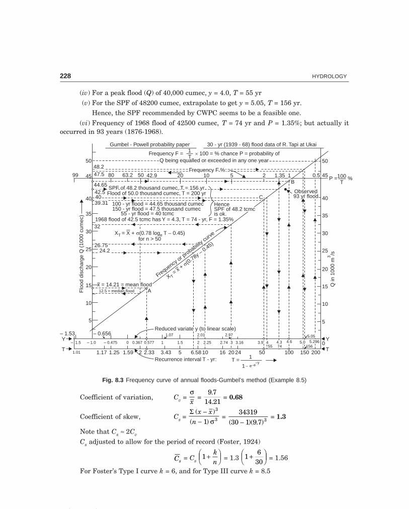
C-9\N-HYDRO\HYD8-1.PM5 228
228 HYDROLOGY
(iv) For a peak flood (Q) of 40,000 cumec, y = 4.0, T = 55 yr(v) For the SPF of 48200 cumec, extrapolate to get y = 5.05, T = 156 yr.
Hence, the SPF recommended by CWPC seems to be a feasible one.(vi) Frequency of 1968 flood of 42500 cumec, T = 74 yr and P = 1.35%; but actually it
occurred in 93 years (1876-1968).
Gumbel - Powell probability paper 30 - yr (1939 - 68) flood data of R. Tapi at Ukai
Frequency F = 100 = % chance P = probability ofQ being equalled or exceeded in any one year
´Frequency F = 100 = % chance P = probability ofQ being equalled or exceeded in any one year
´1T
SPF of 48.2 thousand cumec, T = 156 yrSPF of 48.2 thousand cumec, T = 156 yrFlood of 50.0 thousand cumec, T = 200 yrFlood of 50.0 thousand cumec, T = 200 yr
100 - yr flood = 44.65 thousand cumec
55 - yr flood = 40 tcmc150 - yr flood = 47.5 thousand cumec
1968 flood of 42.5 tcmc has Y = 4.3, T = 74 - yr, F = 1.35%
X = X + (0.78 log T – 0.45)for n > 50
T esX = X + (0.78 log T – 0.45)for n > 50
T es
Frequencyor probability
curve
X= x +
(0.78y – 0.45)
T
s
Frequencyor probability
curve
X= x +
(0.78y – 0.45)
T
s
x = 14.21 = mean floodx = 14.21 = mean flood12.5 = median flood12.5 = median flood
50
45
40
35
30
25
20
15
10
5
– 0.656– 1.53
Flo
oddi
scha
rge
Q(1
000
cum
ec)
26.7526.7524.224.2
3232
39.3139.31404042.542.544.6544.65
9999 47.547.548.248.2
8080 63.263.2 5050 42.942.9 2020Frequency F %Frequency F %
1010 55 22 1.351.35 11 0.50.5 4545
5050
4040
3535
3030
2525
2020
1515
1010
55
YY
TT
BB
CC
P = %100T
HenceSPF of 48.2 tcmcis ok.
HenceSPF of 48.2 tcmcis ok.
Qin
1000
m/s3
5.2965.296 00156156
5.055.05
5.05.04.64.64.34.3443.93.974745555
2002001501501001005050
3.163.16332.742.742.252.25221.51.5
2.012.01 2.972.97
24242020161610106.586.5855
1.071.07
11
3.433.432.332.3322
0.5770.5770.3670.36700
1.591.591.251.25
– 0.475– 0.475
1.171.17
– 1.0– 1.0– 1.5– 1.5
1.011.01
YY
T
Reduced variate y (to linear scale)Reduced variate y (to linear scale)
Recurrence interval T - yr:Recurrence interval T - yr: T =T = 1
1 – e–e–y
Observed93 yr floodObserved93 yr flood
A
Fig. 8.3 Frequency curve of annual floods-Gumbel’s method (Example 8.5)
Coefficient of variation, Cv = σx
= 9 7
14 21..
= 0.68
Coefficient of skew, Cs = Σ ( )( )
x xn
−−
3
31 σ =
3431930 1 9 7 3( )( . )−
= 1.3
Note that Cs ≈ 2Cv
Cs adjusted to allow for the period of record (Foster, 1924)
Cs = Cs 1 +FHG
IKJ
kn = 1.3 1
630
+FHG
IKJ = 1.56
For Foster’s Type I curve k = 6, and for Type III curve k = 8.5


C-9\N-HYDRO\HYD8-2.PM5 229
FLOODS—ESTIMATION AND CONTROL 229
Coefficient of flood, Cf = x
A0.8 0.82 14
14210
62000 2 14/ . ( ) / .= = 4.46
(b) Foster’s Method From the value of Cs , the values of the factor K giving the variations
of the peak flood from the mean flood at various percentages of time (i.e.,, probability P%) canbe obtained by referring to the Tables 8.6 and 8.7 prepared by Foster. From this, the floodfrequency curve can be drawn; and the probability and recurrence interval (T = 1/P × 100) of adesired flood magnitude can be read off from the curve.
In Example 8.5, for Q = 14.21 tcm, σ = 9.7 tcm, Cs = 1.56, from Table 8.6, the flood
frequencies can be determined as follows (tcm = thousand cumec):
Frequency Recurrence Skew curve Variation Flood peakP (%) interval factor K from the QT = Q + Kσ
(T-yr) (from Table 8.6 mean flood (tcm)
for Cs = 1.6) Kσ (tcm)
0.01 10000 5.67 52.1 66.31
0.1 1000 4.75 43.7 57.91
1 100 3.40 31.25 45.46
5 20 2.07 19.05 33.26
20 5 0.69 6.35 20.56
50 2 –0.32 –2.94 11.27
100 1 –0.96 –9.32 4.89
The frequency curve is shown in Figs. 8.4 and 15.1. While the highest flood observed in93 years (1876-1968) is 42.5 tcm, the 100-year flood by Foster’s Type I curve is predicted as45.46 tcm.
Table 8.6 Skew Curve Factors (K values) for Foster’s Type I curve
Cs Frequency P (%)
99 95 80 50 20 5 1 0.1 0.01 0.001 0.0001
0 –2.08 –1.64 –0.92 0 0.92 1.64 2.08 2.39 2.53 2.59 2.62
0.2 –1.91 –1.56 –0.93 –0.05 0.89 1.72 2.25 2.66 2.83 2.94 3.00
0.4 –1.75 –1.47 –0.93 –0.09 0.87 1.79 2.42 2.95 3.18 3.35 3.44
0.6 –1.59 –1.38 –0.92 –0.13 0.85 1.85 2.58 3.24 3.59 3.80 3.92
0.8 –1.44 –1.30 –0.91 –0.17 0.83 1.90 2.75 3.55 4.00 4.27 4.43
1.0 –1.30 –1.21 –0.89 –0.21 0.80 1.95 2.92 3.85 4.42 4.75 4.95
1.2 –1.17 –1.12 –0.86 –0.25 0.77 1.99 3.09 4.15 4.83 5.25 5.50
1.4 –1.06 –1.03 –0.83 –0.29 0.73 2.03 3.25 4.45 5.25 5.75 6.05
1.6 –0.96 –0.95 –0.80 –0.32 0.69 2.07 3.40 4.75 5.67 6.25 6.65
1.8 –0.87 –0.87 –0.76 –0.35 0.64 2.10 3.54 5.05 6.08 6.75 7.20
2.0 –0.80 –0.79 0.71 –0.37 0.58 2.13 3.67 5.35 6.50 7.25 7.80

C-9\N-HYDRO\HYD8-2.PM5 230
230 HYDROLOGY
Table 8.7 Skew Curve Factors (K values) for Foster’s Type-III curve
Cs Frequency P (%)
99 95 80 50 20 5 1 0.1 0.01 0.001 0.0001
0 –2.33 –1.64 –0.84 0 0.84 1.64 2.33 3.09 3.73 4.27 4.76
0.2 –2.18 –1.58 –0.85 –0.03 0.83 1.69 2.48 3.08 4.16 4.84 5.48
0.4 –2.03 –1.51 –0.85 –0.06 0.82 1.74 2.62 3.67 4.60 5.42 6.24
0.6 –1.88 –1.45 –0.86 –0.09 0.80 1.79 2.77 3.96 5.04 6.01 7.02
0.8 –1.74 –1.38 –0.86 –0.13 0.78 1.83 2.90 4.25 5.48 6.61 7.82
1.0 –1.59 –1.31 –0.86 –0.16 0.76 1.87 3.03 4.54 5.92 7.22 8.63
1.2 –1.45 –1.25 –0.85 –0.19 0.74 1.90 3.15 4.82 6.37 7.85 9.45
1.4 –1.32 –1.18 –0.84 –0.22 0.71 1.93 3.28 5.11 6.82 8.50 10.28
1.6 –1.19 –1.11 –0.82 –0.25 0.68 1.96 3.40 5.39 7.28 9.17 11.12
1.8 –1.08 –1.03 –0.80 –0.28 0.64 1.98 3.50 5.66 7.75 9.84 11.96
2.0 –0.99 –0.95 –0.78 –0.31 0.61 2.00 3.60 5.91 8.21 10.51 12.81
2.2 –0.90 –0.89 –0.75 –0.33 0.58 2.01 3.70 6.20
2.4 –0.83 –0.82 –0.71 –0.35 0.54 2.01 3.78 6.47
2.6 –0.77 –0.76 –0.68 –0.37 0.51 2.01 3.87 6.73
2.8 –0.71 –0.71 –0.65 –0.38 0.47 2.02 3.95 6.99
3.0 –0.67 –0.66 –0.62 –0.40 0.42 2.02 4.02 7.25
In the given example, the 1945 flood of 24200 cumec was exceeded in 1959 (when theflood was 37300 cumec), i.e., in 14 years. From the graph for Q = 24200 cumec, T = 6.5 yr (7.75-yr-Weibull); P = 100/6.5 = 15%. The probability that this flood will not occur in the next 14years is
P(N, 0) = (1 – 0.15)14 = 0.10 or 10%and the probability of its occurrence in the next 14 years is
PEx = 1 – 0.1 = 0.90 or 90%but actually it is exceeded after 14 years.
(c) Weibull’s Method The Weibull’s distribution will not give a straight line plot on theGumbel-Powel probability paper and hence can better be plotted on a log-log paper. Both theGumbell’s and Weibull’s curves are plotted on log-log paper in Fig. 8.4 for comparison. It canbe seen that for smaller floods (say, m ≥ 5) both the methods give the same plotting positions ;but for the larger floods (m < 5), the Weibull’s method gives lower recurrence interval, i.e.,largest floods of increased frequency. For example from the Weibull’s frequency curve in Fig. 8.4,for the SPF of 48.2 thousand cumec, T = 48 yr, while by the Gumbel’s method T = 160 yr for thesame SPF); for T = 100 yr, Q = 60 thousand cumec.
(d) Fuller’s formula
Q = CA0.8 (1 + 0.8 log T) (1 + 2.76A–0.3) Q100 = 2.27 (62000)0.8 (1 + 0.8 log 100) [1 + 2.76 (62000)–0.3]
= 40700 cumec (100-yr flood)against Gumbel’s 44650 cumec.

C-9\N-HYDRO\HYD8-2.PM5 231
FLOODS—ESTIMATION AND CONTROL 231
Fig. 8.4
30-yr (1939-68)flood data of
R.Tapi at Ukai
30-yr (1939-68)flood data of
R.Tapi at UkaiFoster stypecurve
¢I
Log-log paper
GumbelFoster IWeibull
GumbelFoster IWeibull
Frequencycurves
Frequencycurves
70 tcmc6047 48.2
44
Flood
150-yr100-yr
48.2 tcm
Flood
150-yr100-yr
48.2 tcm
Weibull
70 tcm60 tcm
Weibull
70 tcm60 tcm
Gumbel
47 tcm44 tcm
Gumbel
47 tcm44 tcm
Foster
50 tcm46 tcm
Foster
50 tcm46 tcm
48-yr(Frequent
high floods)
48-yr(Frequent
high floods)
T = n + 1m
T = 1
1–e–e–y1
1–e–e–y
160-yr160-yr 146-yr146-yr
Q = Q + KK = (c ,T)T Q
s
sf
Q = Q + KK = (c ,T)T Q
s
sf
93-yr
obsd.flood93-yr
obsd.flood
+
48 60
10080
60
40
30
20
15
108
6
4
3
2
1.5
11 1.5 2 3 4 6 8 10 15 20 30 40 60 80100 200 400
300150Recurrence interval (T-yr)
Ann
ualp
eak
flood
sQ
(100
0cu
mec
)
Qin
1000
m/s
T3
1
10
1000.250.51102550100
Frequency F = % = P or % chance of > Q,in any one year
100T
Plotting positionPlotting positionWeibull, 1939Foster, 1924
Gumbell, 1958
Weibull, 1939Foster, 1924
Gumbell, 1958
Foster 1
Fig. 8.4 Log-log plot of flood frequency (Example 8.5)
(e) Creager’s formula
Q = C(0.386 A A) ( ) .0.894 0.386 0 048−
= 140 ( . ) ( ) .0 386 62000 0.894 0.386 62000 0 048
× × −
= 36000 cumec, which was well exceeded in the year 1968 when the peakflood was 42500, cumec.
Hence, the Gumbel’s method gives the most probable maximum flood in the life periodof a structure to be designed and can be adopted in the safe design of hydraulic structures.
(f) World enveloping flood formula (J.M. Baird and J.F. Meillnraith)
Q = 3010
277 0.78A
A( )+ =
3010 62000
277 62000 0.78×
+( ) = 33500 cumec
which was well exceeded in the year 1968.(g) Rational formula
Q = CiA i = design intensity of rainfall (= ic) = 31.8 cm in 3 days during Aug. 4-6, 1968
(See the Introduction part of Chapter 1)C = runoff coefficient = 0.43, from the 3-day storm of Aug. 1968A = 62000 km2 = 62 × 105 ha

C-9\N-HYDRO\HYD8-2.PM5 232
232 HYDROLOGY
Since 1 ha-cm/hr = 1/36 cumec
Q = 1
36 0.43
31.8 cm72 hr
62 10 ha5× × ×FHG
IKJ = 32700 cumec
which has been exceeded in the year 1968. However, the peak flood obtained by the rationalformula depends upon the accuracy of the coefficient of runoff assumed.Example 8.6 Twenty largest one-day floods (without respect to time) are selected in a period of20 years arranged in the descending order of magnitude (cumec). Draw the partial durationcurve:
501, 467, 371, 351, 351, 345, 334, 311, 283, 273,
266, 264, 221, 214, 194, 193, 182, 175, 173, 163.Solution The computations are shown in Table 8.8.
Table 8.8 Computation for partial duration curve
Sl. Flood flow Probable frequency inno. (cumec) 100 years
1 501 5*
2 467 10
3 371 15
4 351 20
5 351 25
6 345 30
7 334 35
8 311 40
9 283 45
10 273 50
11 266 55
12 264 60
13 221 65
14 214 70
15 194 75
16 193 80
17 182 85
18 175 90
19 173 95
20 163 100
*Probable frequency = my
× =1001
20 × 100 = 5
The partial duration curves are plotted on both log-log paper and semi-log paper asshown in Fig. 8.5 (a) and (b) respectively; the 100-yr flood is extrapolated as 640 and 810cumec from the curves (a) and (b), respectively.

C-9\N-HYDRO\HYD8-2.PM5 233
FLOODS—ESTIMATION AND CONTROL 233
100-yr flood = 640 cumecPartial duration
curve
a. Log-log paperPlotting position= 100´m
y
1000800
600
400
300
200
150
10080
60
40
30
20
101 1.5 2 3 4 5 6 8 10 15 20 30 40 60 80100
10
100
1000100101
Flo
odm
agni
tude
,Q(c
umec
)
Partial durationcurve
Partial durationcurve
Plotting position
= 100´my
810 cumec = 100 yrflood
b. Semi-log paper
900
800
700
600
500
400
300
200
100
0
Flo
odm
agni
tude
Q(c
umec
)
0 10 100
100806040302015108654321.51Frequency in 100 years
Fig. 8.5 Plots of partial duration curve (Example 8.6)
Events having a return period of less than 10 years (P < 0.1) based on annual series willoccur more frequently than indicated because the second or third events in some years may begreater than the annual events in other years and have been omitted from consideration. Ifevents that occur frequently (P < 0.1) are important, a partial duration series should be used.The partial duration series includes all events above a base that has been selected to include atleast one event each year.

C-9\N-HYDRO\HYD8-2.PM5 234
234 HYDROLOGY
The partial duration series recurrence interval TPDS is related to the annual seriesrecurrence interval T as
TPDS = 1
1ln ln ( )T T− −Langbein (1949) derived the theoretical relationship between TPDS and T as given below.
Though the relationship varies from region to region, it is significant only for recurrence up to5 years and after that, a difference of 0.5.
TPDS T
0.5 1.16
1.0 1.58
1.45 2.00
2.0 2.54
5.0 5.52
10.0 10.5
20.0 20.5
50.0 50.5
100.0 100.5
In partial duration series, since several occurrences in one year may be selected, thenotion of annual occurrence (Pa) is introduced as
Pa = m/ywhere m = number of occurrences in ‘y’ years and the probability P in ‘per cent of time’ is givenby
P = (1 – e Pa− ) 100and the average recurrence interval T = 1/Pa, and not 1/P
In Example 8.6, a flood of 273 cumec has been exceeded 10 times during a period of 20years. Then itsannual occurrence Pa = m/y = 10/20 = 0.5average recurrence interval T = 1/Pa = 1/0.5 = 2 yr
annual probability P = (1 – e Pa− ) 100 = (1 – e–0.5) 100 = 39.3%.Example 8.6 (a) The highest annual floods for a river for 60 years were statistically analysed.The sixth largest flood was 30,000 cumec (30 tcm).
Determine:
(i) The period in which the flood of 30 tcm may reoccur once(ii) The percentage chance that this flood may occur in any one year
(iii) The percentage chance that this flood may not occur in the next 20 years(iv) The percentage chance that this flood may occur once or more in the next 20 years
(v) The percentage chance that a 50-yr flood may occur (a) once in 50 years, (b) one ormore times in 50 years
C-9\N-HYDRO\HYD8-2.PM5 235
FLOODS—ESTIMATION AND CONTROL 235
Solution (i) Weibull; T = n
m+ 1
= 60 1
6+
= 10.1, say 10 yr
(ii) Percentage chance, i.e., P = 1T
× 100 = 1
10 1. × 100 = 9.9 say 10%
(iii) Encounter probability,
P(N, 0) = (1 – P)N = 11
10 1
20
−FHG
IKJ.
= 0.124 or 12.4%
(iv) PEx = 1 – (1 – P)N = 1 – P(N, 0) = 1 – 0.124 = 0.876 or 87.6%
(v) (a) P = 1T
× 100 = 1
50 × 100 = 2%
(b) P(N, 0) = 11
50
50
−FHG
IKJ = 0.3631
PEx = 1 – P(N, 0) = 1 – 0.3631 = 0.6369, say 64%Example 8.6 (b) Determine the percentage chance that a 25-yr storm may occur
(a) In the next 10 years (b) In the next year itself(c) May not occur in another 15 years
Solution (a) T = 25, PEx = 1 – (1 – P)N, P = 1T
= 1 – 11
25
10
−FHG
IKJ = 0.335 or 33.5%
(b) PEx = 1 – 11
25
1
−FHG
IKJ = 0.04 or 4%, i.e., 1 in 25 chance
(c) P(N, 0) = (1 – P)N = 1
125
15
−FHG
IKJ = 0.542 or 54.2%
Example 8.6 (c) Determine the return period (recurrence interval T) of a flood, which has a10% risk of being flooded (a) in the next 100 years, (b) in the next 50 years.Solution PEx = 1 – (1 – P)N, for risk of being exceededi.e., PEx = 10% = 0.1
(a) 0.1 = 1 – (1 – P)100, (1 – P)100 = 1 – 0.1 = 0.9 1 – P = 0.90.01 = 0.99895, P = 0.00105 = 1.05 × 10⁻³
T = 1P
= 1
105 10 3. × − = 950 yr, say 1000-yr flood
(b) 0.1 = 1 – (1 – P)50, (1 – P)50 = 1 – 0.1 = 0.9 1 – P = 0.90.02 = 0.9979
P = 0.0021 = 2.1 × 10⁻³
T = 1P
= 1
2 1 10 3. × − = 476 Yr, say 500-yr flood.
Note. If a structure has a life period of 50 years and if we can accept a 10% risk of its beingflooded during its life, then we have to design the structure for a return period of T-Yr as follows:
PEx = 1 – (1 – P)50; for 10% risk, PEx = 0.10.1 = 1 – (1 – P)50, (1 – P)50 = 1 – 0.1 = 0.9(1 – P) = (0.9)0.02 = 0.9979

C-9\N-HYDRO\HYD8-2.PM5 236
236 HYDROLOGY
∴ P = 0.0021 = 2.1 × 10⁻³, T = 1 1
10 3P=
× −2.1 = 476 yr
i.e., we have to design the structure for a 476-yr flood and not for a 50-yr flood; if it is designed for a 50yr flood, the risk of failure
PEx = 1 – (1 – P)50 = 1 – 11
50
50
−FHG
IKJ = 1 – 0.9850 = 0.6358 or 63.6%
Example 8.6 (d) The maximum annual floods for the river Tapti at Ukai were statisticallyanalysed for a period of 93 years (1876-1968). The mean annual flood and the standard devia-tion are 14210 and 9700 cumec, respectively.Determine:
(i) The recurrence interval of the highest flood 42500 cumec (in 1968) by Weibull’s methodand what its percentage chance of occurring in (a) in any year, (b) in 10 years ?
(ii) What is the recurrence interval of the design flood adopted by CWPC (49500 cumec)and the highest flood (42500 cumec) by Gumbels method?Solution For the highest flood, its rank m = 1
(i) Weibull: T = n
m+ 1
= 93 1
1+
= 94 yr
(a) P = 1T
= 1
94 = 0.01065 or 1.065%
i.e., its chance of occurrence in any year is ~_ 1%
(b) PEx = 1 – (1 – P)N = 1 – 1
194
10
−FHG
IKJ = 0.1014 or 10.14%, i.e., 10% chance.
(ii) From Gumbel’s Eqn. (8.17 a):(a) Design flood QDF = 49500 cumec = QT , Q = 14210 cumec
QT = Q + σ (0.78 ln T – 0.45), for n > 50 49500 = 14210 + 9700 (0.78 ln T – 0.45) ln T = 5.241, T = 189, say 190 yr
against Weibull’s 50 yr, Fig. 8.4(b) Highest flood QMF = 42500 cumec = QT
42500 = 14210 + 9700 (0.78 ln T – 0.45) ln T = 4.316, T = 75 yr, against Weibull’s 30 yr, Fig. 8.4
Gumbel Frequency Distribution: Resume of formulae:For large values of n, (n > 50):
P = 1 – e e y− −, T =
1P
= 1
1 − − −e e y
yT = – ln . lnT
T −LNM
OQP1
...(8 14a)
yT = – 0 834 2 3031
. . log . log+−
LNM
OQP
TT
...(8.14b)

C-9\N-HYDRO\HYD8-2.PM5 237
FLOODS—ESTIMATION AND CONTROL 237
y = 1
0 78. σ (X – X + 0.45 σ), y = yT , X = Q ...(8.14)
or, y = 12825. ( )X X−
σ + 0.577 ...(8.14c)
i.e., y = a X X( )−
σ + b, a = 1.2825, b = 0.577 ...(8.14d)
XT = X + σ (0.78 y – 0.45) ...(8.17)
XT = X + σ (0.78 ln T – 0.45) ...(8.17a)
XT = X + σ (1.8 log T – 0.45). ...(8.17b)Example 8.6 (e) Statistical analysis of the annual floods of the river Tapti (1876-1968) usingGumbel’s method yielded the 100-yr and 10-yr floods as 42800 and 22700 cumec, respectively.Determine:
(a) the magnitude of a 20-yr flood.(b) the probability of a flood of magnitude 35000 cumec (i) occurring in the next 10 years,
(ii) in the next year itself.
Solution Eq. (8.14a): y10 = – ln . ln 109
= 2.25, X10 = 22.7 tcm
y100 = – ln . ln 10099
= 4.6 , X100 = 42.8 tcm
Eq. (8.14d): 2.25 = a X( . )22 7 −
σ + b ...(i)
4.6 = a X( . )42 8 −
σ + b ...(ii)
(ii)–(i): 2.35 = 20.1 aσ
∴ σ = 20.1 × 128352 35.
. = 10.969 tcm
From Eq. (8.14c): 22.7 – X = (2.25 – 0.577) 10 96912825
..
= 14.309
∴ X = 22.7 – 14.309 = 8.391 tcm
(a) Eq. (8.14a): y20 = – ln . ln 2019
= 2.97
Eq. (8.14c): 2.97 = 1282510 969.
. (X20 – 8.391) + 0.577
X20 = 28.856 tcm or 28856 cumecAlternatively, Eq. (8.17a): X20 = 8.391 + 10.969 (0.78 ln 20 – 0.45) = 29 tcm, or 29000 cumec
(b) Eq. (8.14c): yT = 1282510 969.
. (35 – 8.391) + 0.577 = 3.6881
Eq. (8.14a): – ln . ln T
T − 1 = 3.6881
C-9\N-HYDRO\HYD8-2.PM5 238
238 HYDROLOGY
T = 41 yr, P = 1T
= 0.0244
Alternatively, P = 1 – e e y− − = 1 – e ee− −−
= −3 6881
1 0.025.
= 1 – 0.9753 = 0.0247
T = 1P
= 1
0 0247. = 40.5, say 40 yr
(i) PEx = J(41, 10) = 1 – (1 – 0.0244)10 = 0.2188, say 22%(ii) PEx = J(41, 1) = – (1 – 0.0244)1 = 0.0244, or 2.44% chance
Example 8.6 (f) The annual floods for a large period were statistically analysed by Gumbel’s
methods, which yielded Q = 19000 cumec, σ = 3200 cumec.
Determine(a) the probability of a flood magnitude of 30000 cumec occurring in the next year.
(b) the flood magnitude of 5-yr return period.
Solution (a) y = 128253200.
(30000 – 19000) + 0.577 = 5.5
P = 1 – e e y− −= 1 – e–0.0067 = 1 – 0.9901 = 0.0099 ~_ 1%
PEx = 1 – (1 – 0.0099)1 = 0.0099 ~_ 1%
(b) T = 5, P = 15
= 1 – e e y− −, y = 0.079
0.079 = 128253200.
(X – 19000) + 0.577, X = 17758 cumec
8.6 METHODS OF FLOOD CONTROL
A flood is an unusual high stage of a river overflowing its banks and inundating the marginallands. This is due to severe storm of unusual meteorological combination, sometimes com-bined with melting of accumulated snow on the catchment. This may also be due to shifting ofthe course of the river, earthquake causing bank erosion, or blocking of river, or breaching ofthe river flood banks. Floods have swept vast regions in India, particularly in the basins ofrivers Kosi, Brahmaputra, Godavari, Narmada and Tapti. Floods cause much loss of life andproperty, disruption of communication, damage to crops, famine, epidemic diseases and otherindirect losses.
Design magnitudes of floods are needed for the design of spillways, reservoirs, bridgeopenings, drainage of cities and air ports, and construction of flood walls and levees (floodbanks). The maximum flood that any structure can safely pass is called the ‘design flood’.
The damages due to the devastating floods can be minimised by the following floodcontrol measures, singly or in combination.
(i) by confining the flow between high banks by constructing levees (flood banks) ,dykes, or flood walls.
(ii) by channel improvement by cutting, straightening or deepening and following rivertraining works.
(iii) by diversion of a portion of the flood through bypasses or flood ways. In some casesa fuse plug levee is provided. It is a low section of levee, which when once over topped, will
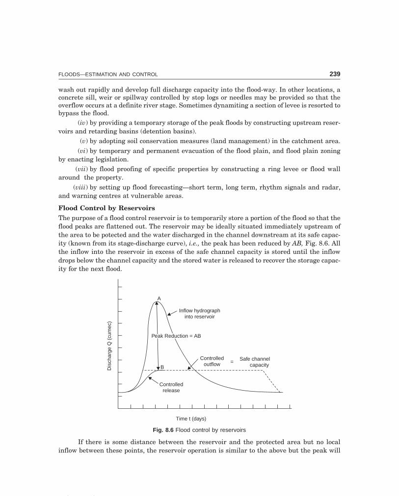
C-9\N-HYDRO\HYD8-2.PM5 239
FLOODS—ESTIMATION AND CONTROL 239
wash out rapidly and develop full discharge capacity into the flood-way. In other locations, aconcrete sill, weir or spillway controlled by stop logs or needles may be provided so that theoverflow occurs at a definite river stage. Sometimes dynamiting a section of levee is resorted tobypass the flood.
(iv) by providing a temporary storage of the peak floods by constructing upstream reser-voirs and retarding basins (detention basins).
(v) by adopting soil conservation measures (land management) in the catchment area.(vi) by temporary and permanent evacuation of the flood plain, and flood plain zoning
by enacting legislation.(vii) by flood proofing of specific properties by constructing a ring levee or flood wall
around the property.(viii) by setting up flood forecasting—short term, long term, rhythm signals and radar,
and warning centres at vulnerable areas.
Flood Control by ReservoirsThe purpose of a flood control reservoir is to temporarily store a portion of the flood so that theflood peaks are flattened out. The reservoir may be ideally situated immediately upstream ofthe area to be potected and the water discharged in the channel downstream at its safe capac-ity (known from its stage-discharge curve), i.e., the peak has been reduced by AB, Fig. 8.6. Allthe inflow into the reservoir in excess of the safe channel capacity is stored until the inflowdrops below the channel capacity and the stored water is released to recover the storage capac-ity for the next flood.
Controlledrelease
ControlledoutflowB
A
Peak Reduction = ABPeak Reduction = AB
Inflow hydrographinto reservoir
Safe channelcapacity
=
Time t (days)
Dis
char
geQ
(cum
ec)
Fig. 8.6 Flood control by reservoirs
If there is some distance between the reservoir and the protected area but no localinflow between these points, the reservoir operation is similar to the above but the peak will
C-9\N-HYDRO\HYD8-2.PM5 240
240 HYDROLOGY
further be reduced due to storage in the reach downstream from the reservoir. If there is asubstantial local inflow between the dam and the control point, the reservoir must be operatedto produce a minimum peak at the protected area rather than at the dam site; otherwise therelease from a reservoir may unfortunately synchronise at some point downstream with floodflows from a tributary. Timely and reliable weather forecasts and prompt information aboutprecipitation upstream and downstream of the reservoir and the means of translation of thisinformation into necessary flood hydrographs will all help in effective reservoir operation.Construction of reservoirs for flood control only is rarely economical and other benefits likeirrigation, hydel power, also have to be taken into consideration. It is the modern practice toconstruct multipurpose reservoirs, where a space is allocated exclusively for flood control,usually above the spillway crest level and is made available when required by closing thespillway crest gates.
The effectiveness of the reservoir in reducing peak flows, increases as its storage capac-ity increases. The maximum capacity required is the difference in volume between the saferelease from the reservoir and the maximum inflow. Since the hydrograph is wider at lowflows, more water must be stored to reduce the peak by a given amount. As the peak reductionis increased, more marginal area will be protected from the floods. The benefits accrued by aunit peak reduction are usually less. Thus, the size of the reservoir has to be determined byweighing the cost involved in reducing the peak with the benefits accrued. A single reservoiracross the main river may not give the required protection to all towns and cities widely lo-cated and reservoirs constructed across tributaries are effective in flood protection. In general,at least one-third of the total drainage area should come under one reservoir for effective floodcontrol.
Retarding BasinsThe release from a storage reservoir is controlled by gates and valves and regulated by theproject engineer. A retarding basin is provided with outlets like a large spillway and sluices
with no control gates. The sluice discharges like an orifice, i.e., Q = CdA 2gH , and there is a
greater throttling of flow when the reservoir is nearly full than would a spillway discharginglike a weir, i.e., Q = CLh3/2 (Fig. 8.7). However, a spillway is necessary for emergency in case ofthe flood exceeding the design maximum.
The discharge capacity of a retarding basin when full should equal the safe dischargingcapacity of the channel downstream. The storage capacity of the basin should be equal to thevolume of the design flood minus the volume of water released during the flood. A retardingbasin is used only for the purpose of flood control. After the peak of flood has passed, the inflowwill gradually become equal to the outflow. One of the limitations of the retarding basins isthat the discharge from the basin may synchronise with the flood flow of a tributary down-stream and as such they are constructed on comparatively small stream while storage reser-voirs are provided across big rivers (since the release can be regulated).
For any pool elevation of the reservoir, the storage and discharge can be calculated. Fora known inflow hydrograph, the corresponding outflow hydrograph can be determined by anymethod of flood routing (Chapter 9).

C-9\N-HYDRO\HYD8-2.PM5 241
FLOODS—ESTIMATION AND CONTROL 241
BL
twlA
Area of c/sBL
Q
MWL
h
HH
Q = C A 2gH + CLhd3/2
Crest Spillway (with nocrest gates) length L
Sluice with bell mouth(ungated) entry
tail water level
Fig. 8.7 Retarding basin
Construction of LeveesThe construction of levees (flood banks or dykes) is extensively followed in India, since it is aneconomical, direct and immediate method. The design and construction of levees are similar tothose of an earth dam. The levees are constructed beyond the meander belt of a river, Fig. 8.8 (a)and they tame a river not to change its course. As far as possible, there should be very fewcurves in their alignment. They require constant watch and after the floods recede, repairsand restoration of levees should be resorted to.
The spacing and height of levees are determined by a series of trials. A height is as-sumed and the discharge through the proper channel is computed for the assumed high waterflow, which is the level of the top of bank less the free board. This flow subtracted from theestimated probable maximum flood discharge gives the discharge to be passed over the floodways between the proper channel and the levees (Figs. 8.8 (a) and (b), 8.9 and 8.10). Area ofthe flood ways is then obtained by dividing it by the velocity of flow. The spacing of levees thusobtained, should give a minimum value for the cost of levees and the value of the submergedland in the flood way. The effects of levees on flood flow are:
(i) increase in the rate of flood flow(ii) increase in the flood water elevation
(iii) increase in the carrying capacity of the channel(iv) increase in the scouring action(v) decrease of surface slope of stream above the leveed section
Channel ImprovementChannel improvement increases the discharging capacity of the stream thereby decreasingthe height and duration of the flood. Flood carrying capacity can be increased either by in-creasing the cross-sectional area or by increasing the velocity along the river. Enlarging thesection is attempted only for narrow and shallow channels with small watersheds, the limit ofsuch enlargement in width being 30-40 m. Deepening is preferred to widening since the hy-draulic mean radius increases more with depth (for the same increase in the sectional area)thus increasing the velocity.

C-9\N-HYDRO\HYD8-2.PM5 242
242 HYDROLOGY
Meanderbelt
Meanderbelt
Meanderingriver
Meanderingriver
Levees
(a) Levees along a meandering river
Design flood level FB TW
2
21
Berms3
11Berm Revetment
31 6
Drain
Borrow pitTrench
FB - Free board, TW - Top width
(b) Typical levee cross section
Fig. 8.8 Flood control by levees
River
City
Ring levee
Tributary
Diversionchannel
Fig. 8.9 Ring levee to protect a city

C-9\N-HYDRO\HYD8-2.PM5 243
FLOODS—ESTIMATION AND CONTROL 243
Reservoir
Dam
River d/sof reservoir
Levee
City
Fig. 8.10 Flood protection by reservoir and levees for a city
The channel velocity (given by Manning’s or Chezy’s formulae) is affected by hydraulicmean radius, slope of river bed and roughness of the bed and sides. Roughness can be reducedby
(i) removing sand bars.(ii) prevention of cropping on river beds near banks.
(iii) removal of fallen trees and other snags.(iv) elimination of sharp bends of meandars by providing cutoffs (Fig. 8.11).In a stream, deepening results in the loss of slope as its outlet can not usually be low-
ered. Deepening can be resorted to only when cutoffs are provided, when the slope of thechannel is increased due to the reduction in the length of flow. Thus, a cutoff helps
(i) in increase the velocity by increasing the slope,(ii) to shorten the path of flow by elimination of meandars, and consequently
(iii) to shorten the levees necessary to confine flood waters.Elimination of meanders by providing straight cutoffs has been done on the river Mis-
sissippi in USA.

C-9\N-HYDRO\HYD8-2.PM5 244
244 HYDROLOGY
Cut-off
Bend gets siltedup later
Fig. 8.11 Cut-off in a meandering river
Example 8.7 A channel has a bottom width of 200 m, depth 6 m and side slopes 1:1. If thedepth is increased to 9 m by dredging, determine the percentage increase in velocity of flow inthe channel. For the same increase in cross sectional area, if the channel is widened (instead ofdeepening), what is the percentage increase in the velocity of flow.
Solution Chezy’s formula, V = C RSwhere V = velocity of flow in the channel
R = hydraulic mean radiusS = bed slope of the channelC = a constant, depending on the roughness of the bed and sidesAssuming the bed slope and roughness are the same in both the cases of deepening and
widening, V ∝ R
Case (i) Increasing the depth to 9 m by dredging.Putting the subscript ‘o’ for the original area of cross section (A), wetted perimeter (P)
and the hydraulic mean radius (R), i.e., before deepening Fig 8.12,A0 = (200 + 1 × 6)6 = 1236 m2
P0 = 200 + 2 × 6 1 12 + = 217 m
R0 = AP
0
0
1236217
= = 5.7 m
After deepening from 6 m to 9 m, Fig. 8.12,A = (194 + 1 × 9)9 = 1827 m2
P = 194 + 2 × 9 1 12 + = 219.4 m
R = AP
= 1827219.4
= 8.33 m
Velocity increase by deepening = 8 33 5 70
5 7
. .
.
− × 100 = 21%
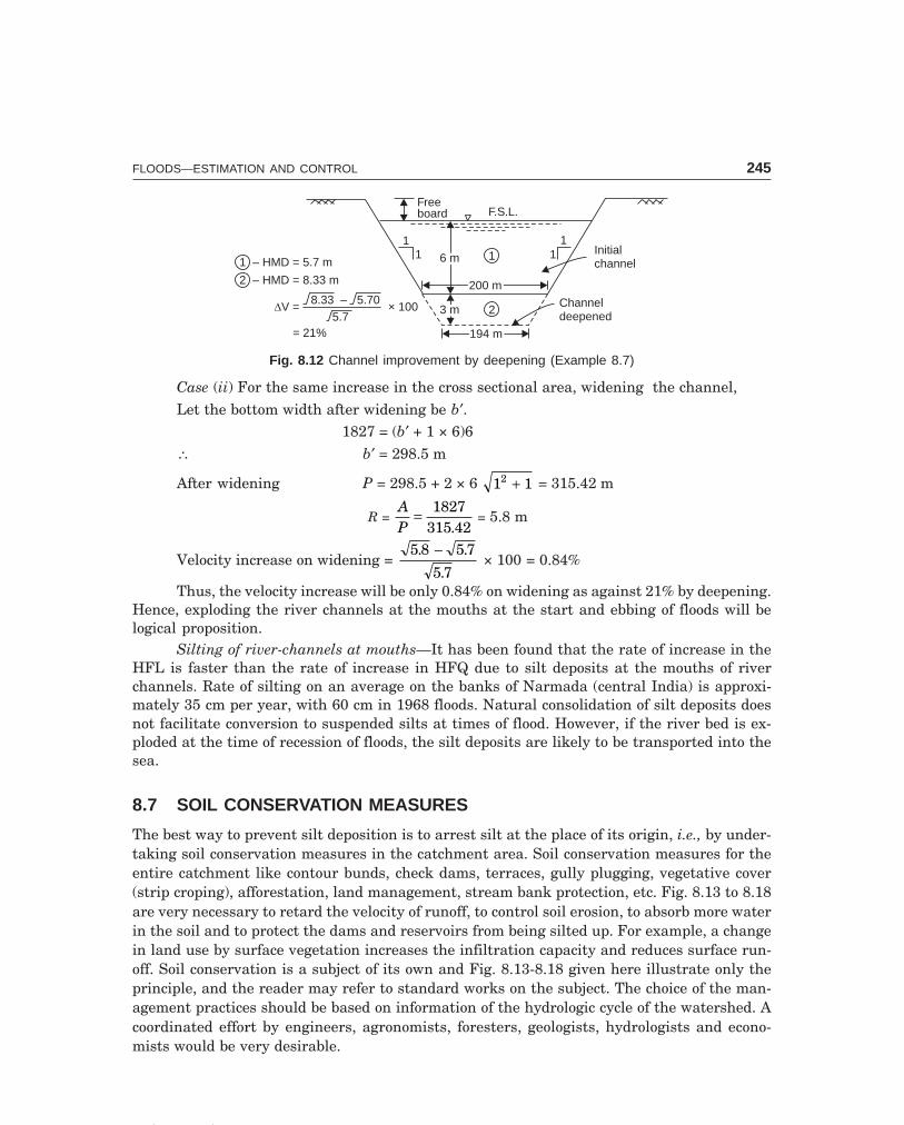
C-9\N-HYDRO\HYD8-2.PM5 245
FLOODS—ESTIMATION AND CONTROL 245
Freeboard F.S.L.
11
1
2
Initialchannel
Channeldeepened
200 m200 m
194 m194 m
3 m3 m
6 m6 m11
1 – HMD = 5.7 m
2 – HMD = 8.33 m
DV = × 1008.33 – 5.70
5.7= 21%
Fig. 8.12 Channel improvement by deepening (Example 8.7)
Case (ii) For the same increase in the cross sectional area, widening the channel,Let the bottom width after widening be b′.
1827 = (b′ + 1 × 6)6∴ b′ = 298.5 m
After widening P = 298.5 + 2 × 6 1 12 + = 315.42 m
R = AP
= 1827315 42.
= 5.8 m
Velocity increase on widening = 5 8 5 7
5 7
. .
.
− × 100 = 0.84%
Thus, the velocity increase will be only 0.84% on widening as against 21% by deepening.Hence, exploding the river channels at the mouths at the start and ebbing of floods will belogical proposition.
Silting of river-channels at mouths—It has been found that the rate of increase in theHFL is faster than the rate of increase in HFQ due to silt deposits at the mouths of riverchannels. Rate of silting on an average on the banks of Narmada (central India) is approxi-mately 35 cm per year, with 60 cm in 1968 floods. Natural consolidation of silt deposits doesnot facilitate conversion to suspended silts at times of flood. However, if the river bed is ex-ploded at the time of recession of floods, the silt deposits are likely to be transported into thesea.
8.7 SOIL CONSERVATION MEASURES
The best way to prevent silt deposition is to arrest silt at the place of its origin, i.e., by under-taking soil conservation measures in the catchment area. Soil conservation measures for theentire catchment like contour bunds, check dams, terraces, gully plugging, vegetative cover(strip croping), afforestation, land management, stream bank protection, etc. Fig. 8.13 to 8.18are very necessary to retard the velocity of runoff, to control soil erosion, to absorb more waterin the soil and to protect the dams and reservoirs from being silted up. For example, a changein land use by surface vegetation increases the infiltration capacity and reduces surface run-off. Soil conservation is a subject of its own and Fig. 8.13-8.18 given here illustrate only theprinciple, and the reader may refer to standard works on the subject. The choice of the man-agement practices should be based on information of the hydrologic cycle of the watershed. Acoordinated effort by engineers, agronomists, foresters, geologists, hydrologists and econo-mists would be very desirable.

C-9\N-HYDRO\HYD8-3.PM5 246
246 HYDROLOGY
Land surface
Gulley becomesdeeper and wider if
uncheckedc. Gulley c/s
Gully(Due to land
erosion)
Retainingwall
a. Plan
Bottomof gully
GulleyBoulders
Retainingwall
b. c/s of gulley and retaining wall
Fig. 8.13 Gully plugging
Dam
Reservoir
C
Main stream
C C
C
CTributariesTributaries
Catchmentarea
C-Check dam
a. Plan
b. L/S of stream
Stream bed
Water surface
Check dam
Fig. 8.14 Check dams

C-9\N-HYDRO\HYD8-3.PM5 247
FLOODS—ESTIMATION AND CONTROL 247
Flood plain zoning Areas, very near to the river are the most vulnerable and thereforeshould not be allowed to be used for building houses. They may be used for parks, recreationgrounds, etc. so that inundation of such land may not result in loss of human lives or anysignificant damage to property. Raising place for habitations above flood heights can be viewedas an adjunct to embankments.
GW
cul
cul
cul
cul
c
c
c
c
C-ContoursCul-Cultivated
Gw-Grass waterway
Strips of close-growingcrops (grasses & legumes)
Fig. 8.15 Contour farming
3-7.5 m3-7.5 m 3-6 m3-6 m
Filling
Excavation40-50 cm
Original land slope
Fig. 8.16 Contour terrace
112
1
Contour trenches atcertain vert. interval
Tree planted in trench @ 1.5 m c.c.
Bank
Land slope
Fig. 8.17 Contour trenching
8.8 FLOOD CONTROL ECONOMICS
In a flood control project, the degree of flood protection (i.e., to the required stage) should bejustified by an economical analysis of the costs involved in raising the structure to the requiredheights (say, the height of spillway) and the direct and indirect benefits obtained by flood

C-9\N-HYDRO\HYD8-3.PM5 248
248 HYDROLOGY
protection up to that stage. Generally, the flood stage for which the ratio annual benefits tocost is a maximum is adopted for the design of the flood protection works (Fig. 8.19). Protectionagainst floods of rare occurrence is uneconomical because of the large investment (for a smallincrease in the benefits) and hence there is always a certain amount of flood risk involved.
Top of bund
Retaining wallWaste weir
a. Plan
A
A
Land slope
0.9 m0.9 m
0.6 m
b. c/s of bund on AA
112
1 1
112
Fig. 8.18 Contour bund
Max.benefits
Total benefits 2
1 Total costs
Marginal increasein benefit
Marginal increasein benefit
BenefitsCosts
= 1
Design stage offlood protectionDesign stage offlood protection
QD Q = Max. feasible floodpeak reduction cumec
P
1To
talc
osts
,Rs.
incr
ores
2To
tal b
enef
its, R
s.in
cror
es
Reduction in flood peak Q (cumec)
Fig. 8.19 Cost-benefit analysis for design stage of flood protection
The flood control costs include:(i) Capital costs involved in the construction of the structure to the required flood height
(i.e., to offer the required degree of flood protection, say, by a combination of dam-spillway, levees and channel improvement)
(ii) Interest cost on capital expenditure(iii) Sinking fund, depreciation and taxes(iv) Operational expenses and maintenance costThe benefits of flood control include(i) Direct or primary benefits accruing from prevention of flood damages to structures
downstream, losses arising from disruption of communication, (and business), loss of life andproperty, damage to crops, etc.

C-9\N-HYDRO\HYD8-3.PM5 249
FLOODS—ESTIMATION AND CONTROL 249
(ii) Indirect benefits resulting from the money saved under insurance and Workmen’scompensation laws, higher yields from intensive cultivation of protected lands and reductionin flood-prone epidemic diseases, etc.
Assessment of potential flood damage is an important requirement in any organisedflood control programme. Generally stage-damage curves are plotted to show that damage in aparticular region in relation to the rising flood stages in that reach. Indirect damage by floodsdeals with the loss of business and services to community. This is a socioeconomic loss and isdifficult to assess because of the various economic and physical factors involved whereas thedirect damages can be estimated in terms of money value. An assessment of the damagescaused by floods can be made when the data is collected and presented in the following form:
(i) Area affected (km2)(ii) Population affected (lakhs)
(iii) Crops affected(a) in hectares(b) value in rupees
(iv) Damage to property(a) number of houses damaged(b) cost of replacing or repairing in rupees
(v) Loss of livestock(a) category number(b) value in rupees
(vi) Human lives lost(vii) Damage to public works in rupeesSuitable flood indices have to be developed from year to year to enable comparison to be
made of the various flood damages.
Combination of Flood Control MeasuresThe object of a flood-control study is to decide which of the flood control measures, singly or incombination, are most suited and their location, size, design and costs. The design of floodcontrol works should be closely related to the hydrological features and economic justificationof the project.
Suppose the flood control project involves the construction of a reservoir, levees andchannel improvement works, the factors governing the final selection of various combinationsare illustrated in Fig. 8.20. The cost of construction of reservoir to reduce the design flood tovarious lower peaks is indicated by curve (1). The cost of construction of levees and otherchannel improvement works for protection against various flood peaks is indicated by curve(2). The sum of the ordinates of the two curves indicates the combined cost of flood protectionby reservoirs, levees and channel improvement works and is given by the curve (3). Theminimum point P of the combined cost curve represents the most economic combination. Thereduced flood peak and the total cost of works can be read off at this point.
See also Appendix-C: Reservoir Design Studies.

C-9\N-HYDRO\HYD8-3.PM5 250
250 HYDROLOGY
Min.cost
3 Combined cost
1
Cost ofreservoir
Total cost ofproject
2 Cost oflevee &channel
improvement
Designflood peak2
Cos
tofl
evee
&C
h-im
p.(R
s.in
cror
es)
1C
ost o
f res
ervo
ir(R
s.in
cror
es)
3C
ost o
f pro
ject
(Rs.
incr
ores
)
Peak flood Q (1000 cumec)
QD
P
Fig. 8.20 Cost analysis for combination of flood control measures
Example 8.8 The costs of construction of levees for flood protection for various flood peaks aregiven below. From this and other data given, make an economic analysis of the flood controlproject and determine the flood peak for which the levees have to be designed.
Flood peak Total damage Recurrence interval Annual project(1000 cumec) under the flood of flood peak cost up to the
peak (yr) flood peak(Rs. in crores) (Rs. in crores)
10 0 2 0.2
15 2 10 0.4
20 5 20 0.6
25 8 30 0.8
30 12 42 1.0
35 20 60 1.3
40 32 80 1.6
50 46 150 1.8
60 70 300 2.0
70 98 600 2.4
Solution The economic analysis is made as shown in Table 8.5 on the basis of benefit-costratio.
The ratio of benefit to cost is a maximum of 1.39 when the levees are constructed tosafely pass a flood peak of 40000 cumec (Fig. 8.21). Hence, the levees designed for this floodpeak will be most economical.

C-9\N-HYDRO\HYD8-3.PM5 251
FLOODS—ESTIMATION AND CONTROL 251
4.0
3.5
3.0
2.5
2.0
1.5
1.0
0.5
0
1.6
1.4
1.2
1.0
0.8
0.6
0.4
0.2
00 10 20 30 40 50 60 70 80 900 100
Flood peak Q, cumec
2
1
3
AnnualbenefitsAnnualbenefits
Annualcosts
Annualcosts
Design floodpeak
Design floodpeak
BenefitCost
ratio
BenefitCost
ratio = 1.37maximum
Flood protectionby levees
3B
enef
it-co
stra
tio
1A
nnua
l ben
efits
,Rs.
incr
ores
2A
nnua
l cos
ts,R
s.in
cror
es
Fig. 8.21 Benefit-cost analysis (Example 8.8)
8.9 FLOOD FORECASTING AND WARNING
The flood forecasts are issued on the basis of the analysis of weather charts and indicate thelikelihood of heavy rainfall over the specified areas with the next 24 to 48 hours. All Indiaforecasts are prepared every day at Poona.
Radar is very effective in the detection and tracking of severe storms. Meteorologicalsatellites give an excellent idea of the cloud cover over the whole of India and neighbouringcountries.
After the formulation of forecast, it must be dessiminated amongst persons concernedat the fastest speed. This can be done by utilising all available media of communications liketelegraph, teleprinter, telephone and wireless and organising a hierarchy for onward trans-mission, if necessary.
One of the methods of forecasts in The Bureau of Meteorology, Australia comprises thefollowing procedural steps:
(i) Collection of previous 24-hour rainfall in respect of each catchment(ii) Updating the Anticident Moisture Index
(iii) Working out the average depth of rainfall(iv) Assessment of likely extent of the rain from weather charts(v) Collection of river stages
(vi) Issue of preliminary warnings with all factual data collected at every 6-hour interval;the final advice is issued using the crest relationship.
A schematic diagram of the flood forecasting and warning system contemplated for theTapti basin (central India) is given in Chart 8.1.

C-9\N-HYDRO\HYD8-3.PM5 252
252 HYDROLOGYF
lood
pea
kT
otal
dam
age
Incr
emen
t of
Rec
urr
ence
Incr
emen
tA
nn
ual
ben
efit
Tot
al a
nn
ual
An
nu
al p
roje
ctR
atio
af
(100
0 cu
mec
)fo
r th
e pe
akd
amag
ein
terv
al o
fin
rec
urr
ence
from
pro
tec-
ben
efit
s fr
omco
st f
or t
he
ben
efit
(Rs.
cro
res)
(Rs.
cro
res)
floo
d p
eak
inte
rval
tion
of
incr
e-pr
otec
tion
for
floo
d p
eak
to c
ost
(Yr)
(Yr)
men
tal
dam
age
floo
d p
eak
(Rs.
cro
res)
(7)
÷ (8
)R
s. c
rore
s(R
s. c
rore
s)(3
) ÷
(5)
12
34
56
78
9
100
20
0.2
0
28
0.25
152
100.
250.
40.
62
310
0.30
205
200.
550.
60.
92
310
0.30
258
300.
850.
81.
06
412
0.33
3012
421.
181.
01.
18
818
0.44
3520
601.
621.
31.
25
1220
0.60
4032
802.
221.
61.
39
1470
0.20
5046
150
2.42
1.8
1.34
2415
00.
16
6070
300
2.58
2.0
1.29
2830
00.
09
7098
600
2.67
2.4
1.10
Tab
le 8
.9 E
cono
mic
ana
lysi
s of
flo
od c
ontr
ol—
by c
onst
ruct
ing
leve
es (
Exa
mpl
e 8.
8)

C-9\N-HYDRO\HYD8-3.PM5 253
FLOODS—ESTIMATION AND CONTROL 253
Wireless sets invulnerable areas-
10 nos.
Municipalauthorities
Shahada
Dhulia
Malegaon
Akola
Talegaon
Chalisgaon
Burhanpur
Bhusaval
Nanded
Sindkheda
Taloda
Ukai
Kakrapur
Kathor
Flood forecastingcell surat
Focal officer
Collecter
Burhanpur
Bhusaval
Nanded
Sindkheda
Taloda
Ukai
Kakrapur
Kathor
KhandwaSurat
Municipalauthorities
D.S.P.
Stream gauging &wireless stns. u/s
Raingauge stns.in catchment
Radio wind &radio sonde stns.
Chart 8.1 Flood forecasting system in Tapti basin (after B.S. Rao, 1969)
The flood warning system basically means the working out of the flood hydrograph at agiven point sufficiently in advance, given the flood hydrograph of some gauge or gauges suffi-ciently upstream, taking into consideration.
(i) the effect of the incidence of rainfall forecast for or that has fallen in the interveningcatchment and the consequent contribution of floods enroute, and
(ii) the moderation affected by the valley storage from the upstream gauge to the pointunder consideration.
The flood warning system is prepared by(i) forecasting crest height and time.
(ii) flood routing techniques.With a properly developed system of scientific flood forecasting and warning, human
toll and destruction to movable properties could be greatly mitigated.Summary—The various steps involved in the design of a flood control project are:(i) Determination of the project design flood and flood characteristics of the basin.
(ii) Assessment of flood damages for different flood stages and socio-economic problemsinvolved.
(iii) Field survey of flood-prone areas and defining areas to be protected.

C-9\N-HYDRO\HYD8-3.PM5 254
254 HYDROLOGY
(iv) Determination of the possible methods of flood protection.(v) If flood control is feasible by construction of reservoirs and levees, selection of suit-
able sites and their physical characteristics.(vi) Design details of the flood control structures proposed and preparation of cost esti-
mates.(vii) For a combination of flood control measures, selection of a flood peak that offers the
desired protection at minimum cost.(viii) Making the cost-benefit analysis of the project and its economic justification.
(ix) Development of a scientific flood forecasting and warning system.(x) Preparation of a detailed project report, indicating the alternative flood control meas-
ures explored, the combination finally selected with the economic justification for the same,and the degree of flood protection offered.
(xi) Construction of the project proposed after approval and sanction of the budget fromthe authority concerned.
���������
I Match the items in ‘A’ with the items in ‘B’ (more than one item may fit in ‘B’)
A B(i) Floods (a) South India
(ii) SPF (b) Central India(iii) Design storm (c) Maharashtra State(iv) Maximum flood discharge (d) U.S.A.(v) Ryves formula (e) Flood frequency as a factor in flood-estimation
(vi) Dicken’s formula (f) Flood control(vii) Inglis formula (g) Construction of a cofferdam
(viii) Fuller’s formula (h) ≈ twice coefficient of variation (2Cv)(ix) Creager’s formula (i) Increase HMD by deepening(x) Annual flood series (j) Rational formula
(xi) Partial duration series (k) Moisture adjustment(xii) Coefficient of skew, Cs (l) Spillway design flood
(xiii) Retarding basins (m) High intensity of rainfall(xiv) Channel improvement (n) 80% of MPF
II Say ‘True’ or ‘False’; if false, give the correct statement:(i) Floods are caused by succession of high intensity storms on a basin.
(ii) The design flood is taken as the maximum probable flood that may occur on a basin.(iii) The maximum probable flood includes the extremely rare and catastrophic floods and is
usually considered for the spillway design of very high dams.(iv) The standard project flood is a fare estimate of the flood resulting from the most severe
combination of meteorological and hydrological conditions of the basin.(v) The PMP is derived from the most critical combination of storms and moisture adjustment
which, after minimising losses, when applied on the design unit hydrograph for the basin,will produce the MPF.

C-9\N-HYDRO\HYD8-3.PM5 255
FLOODS—ESTIMATION AND CONTROL 255
(vi) The MPF for a basin is usually around 80% of the SPF.
(vii) In flood control project, 100% flood protection is provided and hence there is absolutely noflood risk.
(viii) In a partial duration series, there may be 2–3 high floods of the same year and does not givea true distribution series.
(ix) Annual series are useful during the construction period of a large dam project, while thepartial duration series are preferred for the spillway design flood.
(x) The critical (design) intensity of rainfall occurs when the duration of storm is more than theconcentration time.
(xi) When enough storm data for a basin is not available, the PMP is estimated by storm transpo-sition from a neighbouring catchment which is meteorologically homogeneous.
(xii) The Gumbel distribution provides a satisfactory fit for partial duration foods or rainfall data.
(xiii) While the annual floods are plotted against their probability of their occurrence in 100 years,the partial duration floods are plotted against percentage of time.
(xiv) In channel improvement (for flood control), widening is preferred to deepening.
(xv) While Radar gives an excellent idea of cloud cover, the meteorological satellites are veryeffective in the detection and tracking of severe storms.
(xvi) A flood forecasting and warning system basically means working out of the flood hydrographat a given point sufficiently in advance, given the flood hydrographs at sufficiently upstreampoint/s.
(xvii) The design flood is usually selected after making a cost-benefit analysis.
(xviii) Land management is ineffective in flood control.
(xix) If a certain flood occurs once in 50 years, then its chance of occurring in any one year is 2%.
(xx) Generally, the flood stage (flood peak) for which the ratio of annual benefits to cost is amaximum is adopted for the design of flood protection works.
(xxi) The 100-pr flood will be equalled or exceeded 10 times in a 1000 year period.
(xxii) Protection against rare floods is uneconomical and hence there is always a certain amount offlood risk involved.
(xxiii) The first to suggest that frequency should be considered as a factor in estimating flood was:
(a) Allen Hazen (b) Gumbel
(c) Fuller (d) Weibull
(false: ii, vi, vii, ix, x, xii, xiii, xiv, xv, xviii)
III Classify the following into tangible (direct) and intangible (indirect) benefits due to flood control.
(i) Prevention of damage to structures
(ii) Loss of life and property
(iii) Money saved under insurance and Workmen’s Compensation Laws
(iv) Higher yields from intensive cultivation of protected lands
(v) Elimination of losses arising from interruption of business (due to disruption of communica-tion)
(vi) Reduction in flood-prone epidemic diseases
(vii) Damage to crops.
IV Choose the correct statement/s in the following:
1 The methods of estimating high flood discharge are
(i) by applying PMP on the design unit hydrograph for the basin.
C-9\N-HYDRO\HYD8-3.PM5 256
256 HYDROLOGY
(ii) By empirical formulae developed for the regions.
(iii) By applying rational formula.
(iv) By flood frequency studies.
(v) By stochastic methods.
(vi) From the percent flood risk that can be allowed in the project.
(vii) All the above methods.
2 The methods of mitigating floods are
(i) by construction of reservoirs across tributaries
(ii) by construction of a large reservoir across the main stream
(iii) by construction of a retarding basin across a large river with a tributary joining the riverdownstream
(iv) by construction of levees, flood banks and dykes
(v) by channel improvement
(vi) by land management
(vii) by temporary evacuation of low lying areas and flood warnings
(viii) all the above methods.
3 The ‘design flood’ is taken as
(i) flood peak derived by applying PMP on the design unit hydrograph
(ii) 80% (approx.) of MPF
(iii) SPF
(iv) the flood of the recurrence interval corresponding to the percent risk that can be allowed inthe project
(v) the flood stage for which the ratio of benefit to cost is maximum
(vi) the 25-year flood for a land drainage project
(vii) the 160-year flood for a spillway design or bridge
(viii) all the above. (1–except vi, 2–i, iv, v, vi, vii; 3 vii).
�������
1 (a) Explain ‘design flood’. Is this the same as ‘maximum probable flood’ ?
(b) What are the methods of estimating maximum flood discharge? Give three formulae for maxi-mum flood estimation in India indicating for which part of the country they are applicable.
(c) Find the value of the constants C and n in the empirical formula Q = CAn*, where Q is theflood discharge in cumec and A is the catchment area in km2 from the following data:
A (km2): 4 10 50 100 200
Q (cumec): 100 158 354 500 706
(Hint Plot Q vs. A on log-log paper; C = 50–intercept; n = 0.5 slope of straight line;
Q = 50 A )
2 The design storm for a basin has the depth of rainfall for successive hours as 5.6, 7.6 and 5.2 cm.The 1-hr design unit hydrograph for the basin may be approximated by a triangle of base 6 hourswith a peak of 60 cumec occurring at the 2nd hour from the beginning. Compute the floodhydrograph assuming an average loss rate of 0.5 cm/hr. Base flow may be neglected.

C-9\N-HYDRO\HYD8-3.PM5 257
FLOODS—ESTIMATION AND CONTROL 257
3 (a) Explain the following terms with reference to frequency studies:
(i) Annual series (ii) Partial duration series
(iii) Recurrence interval
(b) At a particular gauging station, the annual maximum floods are recorded from 1951 to 1975.The mean and standard deviation of these floods are 310.24 cumec and 110.54 cumec, respec-tively. Assuming that the flood series follow Gumbel’s distribution, determine the floodmagnitudes for the recurrence intervals of 200, 100, 50 and 25 years. Plot these points on theGumbel’s probability paper.
4 (a) Differentiate: deterministic, probabilistic and stochastic processes in estimation of maxi-mum annual rainfall or flood.
(b) Records of peak flow are available for a river at a station where a reservoir is to be con-structed for a period of 75 years. The arithmetic mean of the peaks is 8200 cumec and thestandard deviation is 3170. Making use of Gumbel’s method determine the recurrence inter-val for a flood of 18400 cumec.
5 (a) Define ‘Recurrence interval’ and ‘Frequency’ as applied to annual floods or rainfall.
(b) What should be the recurrence interval of a flood such that the probability of its occurrencein a 10-year period is 0.01?
(c) The mean of the annual maximum floods at a gauging station with 40 years of records is1300 cumec and the variance is 1620 cumec. Estimate the magnitude of the 100-year flood.
(Hint: variance = square of standard deviation, σ2)
6 The annual flood peaks for Nagavalli river at Thottapalli are given for the period 1930-1950.
(i) Plot the recurrence interval versus flood peak
(ii) From the plot, determine the magnitudes of 50-yr and 100-yr floods.
(iii) What is the recurrence interval of a flood magnitude of 300 cumec?
Year Flood (cumec) Year Flood (cumec)
1930 1065 1941 910
31 645 42 750
32 1005 43 930
33 1350 44 750
34 860 45 1070
35 150 46 830
36 2260 47 1095
37 650 48 384
38 2840 49 2230
39 990 1950 3210
1940 870
7 The maximum annual floods for a river for 26 years are given below:
(i) Plot the frequency curve.
(ii) Determine the magnitude of a 100-yr, 50-yr and 20-yr floods.
(iii) What is the recurrence interval of a flood of 300 cumec?

C-9\N-HYDRO\HYD8-3.PM5 258
258 HYDROLOGY
Year Flood (cumec) Year Flood (cumec)
1955 375 1968 219
56 199 69 490
57 232 70 233
58 419 71 141
59 245 72 256
60 411 73 308
61 166 74 575
62 232 75 229
63 206 76 260
64 232 77 387
65 238 78 283
66 440 79 221
1967 180 1980 250
8 The maximum annual floods for a river for 60 years were statistically analysed. The sixth larg-est flood (i.e., No. 6 when arranged in the descending order of flood magnitude) was 480 cumec.
Determine:
(i) the period in which the flood (i.e., 480 cumec) may reoccur;
(ii) the percentage chance that the flood (i.e., 480 cumec) may occur in any one year.
(iii) the percentage chance that the flood (i.e., 480 cumec) may not occur in the next 20 years.
(iv) the probability that the flood (i.e., 480 cumec) may occur in the next 10 years.
9 (a) What do you understand by degree of protection in relation to a flood control scheme andwhat factors govern the degree of protection to be offered ?
(b) What is the probability that only one flood equal to or exceeding the 50-year flood will occurin a 50-year period? What is the probability that one or more floods equal to or exceeding the‘50-year flood’ will occur in a 50-year period? (2, 64%)
10 (a) Discuss the validity of the probability method of flood estimation. List the demerits, if any.
(b) Compute the magnitude of the return period of a design flood to provide 60% assurance that
failure of a structure would not occur. (2 12 year)
11 What return period must a highway engineer assume in his design of a culvert, if he allows a10% risk that flooding will occur in the next 5 years? (48.1 yr)
12 Explain briefly how you would compute the design flood for a spillway in a reservoir. Assumethat rainfall-runoff data are available for the basin for about 50 years. You may list out thevarious methods available and explain any one of them.
13 The maximum annual floods for River Tapti for 93 years (1876 to 1968) were statistically ana-lysed, and 17 highest annual floods are given below. Draw the frequency curve and determine:
(i) the recurrence interval of the highest flood, SPF of 48200 cumec and the design flood of49500 cumec.
(ii) the 200-yr, 150-yr, 100-yr and 75-yr flood magnitude.
(iii) the probability that the flood of 37300 cumec (a) may not occur in the next 10 years (b) mayoccur in any one year; examine how for case (a) is true.

C-9\N-HYDRO\HYD8-3.PM5 259
FLOODS—ESTIMATION AND CONTROL 259
Maximum annual floods (when water levels at Surat exceeded gauge level 95)of river Tapi during 1876 to 1968
Year Month and date Peak flood(1000 cumec)
1876 Aug. 29 to Sept. 5 21.2
1882 Sept. 12 21.8
1883 July 3 30.2
1884 Sept. 9 24.9
1894 July 22 23.6
1914 Sept. 17 21.8
1930 Sept. 30 22.6
1933 Sept. 18 25.5
1937 Sept. 10 20.0
1942 Aug. 6 22.8
1944 Aug. 18 & 24 (2 peaks) 29.3
1945 Sept. 24 24.2
1949 Sept. 17 18.3
1958 Sept. 2 19.6
1959 Sept. 17 37.3
1962 Sept. 15 22.6
1968 Aug. 6 42.5
Hint Since all the 93 annual floods are not given, it is not possible to determine Q and σ for
Gumbel’s method and hence draw the frequency curve of Weibull’s.
(94, 180, 210 yr; 49, 46, 43, 40 T cumec; 14.8, 85.2% but has been exceeded in 1968 after 9 years).‘PDS’ cannot be applied since there are only 17 events in 93 years.
14 (a) Explain the different methods of avoiding damage by floods
(b) Explain with a neat sketch how flood control is effected by reservoirs with regard to (i) theirnumber, (ii) location, (iii) size, and (iv) operation.
(c) Is land management effective in flood control?
15 (a) Explain the ‘tangible and non-tangible’ benefits due to flood control.
(b) Suppose that a flood control project is to be a combined one and involves the construction ofa reservoir and levees with channel improvement, explain how would you determine themost economic combination of these procedures.
(c) Given below is the information regarding flood stage, recurrence interval, total damage andcost of project for giving protection against indicated stage. Work out the benefit-cost ratioand net benefits (i.e., benefits – costs). What is the peak stage against which you wouldchoose to provide protection?

C-9\N-HYDRO\HYD8-3.PM5 260
260 HYDROLOGY
Peak Total damage Return period Annual cost ofstage below indicated (years) project(m) stage (Rs. in millions)
(Rs. in millions)
9 0 7 0.8
10 8 10 1.2
11 20 15 1.6
12 40 22 2.0
13 64 30 2.6
14 90 70 3.2
15 120 150 3.6
16 160 300 4.0
16 (a) Explain stage by stage the studies to be made and the field work to be undertaken for prepar-ing an estimate and report for a flood control project.
(b) Write a note on ‘flood forecasting and warning’.
17 Write short notes on:
(a) PMP (b) Flood forecasting and warning
(c) Rational formula for flood estimation (d) Design flood
(e) Moisture adjustment (f) Retarding basin
(g) Fuse plug levee (h) Storm transposition
(i) Flood embankment
18 Statistical analysis of an annual flood series for the period 1876–1968 at a station X on the riverTapti shows that the 100-yr flood has a magnitude of 42800 cumec and a 10-yr flood a magni-tude of 22700 cumec. Assuming that the flood peaks are distributed according to the theory ofextreme values, determine
(a) the magnitude of a 20-yr flood.
(b) the probability of a flood equal to or greater than 35000 cumec occurring
(i) in the next 10 years,
(ii) in the next year itself.
(c) the probability of having at least one 10 year flood in the next 4 years.
(d) the mean (Q ) and standard deviation (σ) of the annual floods.
19 A cofferdam has to be built in a river to withstand four consecutive flood seasons (i.e., 4 years)and offer protection against a 20-yr flood. The annual flood series for a period of 30 years at thesite indicate a maximum flood peak of 8000 cumec and a minimum of 1800 cumec. Assumingthat the annual flood peaks plot as a straight line on a semi-log paper (recurrence interval plot-ted as abscissa to logarithmic scale), estimate the magnitude of the 20-yr flood (without plotting)and determine the probability of its occurrence during the life of the cofferdam.
(7200 cumec, 18.6%)

C-9\N-HYDRO\HYD8-3.PM5 261
FLOODS—ESTIMATION AND CONTROL 261
20 The annual rainfall distribution during a period of 75 years of record at a place is given below.
Rainfall range No. of years
<15 cm 5
15-24 cm 12
25-34 cm 18
35-44 cm 30
≥45 cm 10
Determine
(a) the probability of having a rainfall in excess of 45 cm in any one year.
(b) the probability of the rainfall exceeding 45 cm in three successive years,
(c) the probability of occurrence of rainfall of less than 20 cm during the next year.
21 In a tropical area where there are short storms more or less uniformly distributed throughoutthe year. there is a 60% chance of rain on any one day. Determine: (i) the probability that therewill be no rain on any two successive days, (ii) the probability that it will rain on both days, and(iii) that it well rain on only one of the two days.
22 In a certain river, a flood discharge of 2000 cumec was exceeded 48 times during a period of 27years and a flood of 8000 cumec exceeded twice. Determine their annual probability and averagerecurrence interval. (80%, 0.56–yr, 7%, 14–yr)
23 What return period a Municipal Engineer should adopt in the design of a culvert on a drain, if heis willing to accept only a 10% risk of being flooded during the 25 years of the expected life of theculvert? [238 yr]
24 A 45 min storm produces 30 mm of rain over a catchment of 120 ha. If the time of concentrationis 30 min and runoff coefficient is 0.3, estimate the resulting peak flow rate.
[Hint Use eqs. 8.9 & 8.10.] (Ans. 4.663 cumec)
25 The annual floods of a basin were statistically analysed using Gumbel’s distribution which yielded
Q = 32000 cumec, and σ = 6000 cumec. Determine
(a) the recurrence interval of a flood of magnitude 40000 cumec.
(b) the probability of the above flood occurring in the next 5 years. (Ans. 33.33 yr, 14.1%)
26 The annual floods of River Chambal at Gandhisagar dam were statistically analysed which yieldedthe 50-yr and 100-yr floods as 40.8 tcm and 46.3 tcm, respectively. Estimate the 500-yr floodmagnitude. What is the probability that this flood may occur in the next 100 years.
(tcm = 1000 cumec) (Ans. 59 tcm)
27 The annual floods of a river at a particular site were analysed by Gumbel’s method which yielded
Q = 1200 cumec and σ = 650 cumec. For what discharge you design the structure at this site for
95% assurance that the structure would not fail in the next 50 years. (Ans. 4200 cumec)

9.1 RESERVOIR ROUTING
Flood routing is the process of determining the reservoir stage, storage volume of the outflowhydrograph corresponding to a known hydrograph of inflow into the reservoir; this is calledreservoir routing. For this, the capacity curve of the reservoir, i.e., ‘storage vs pool elevation’,and ‘outflow rate vs. pool elevation’, curves are required. Storage volumes for different poolelevations are determined by planimetering the contour map of the reservoir site. For exam-ple, the volume of water stored (V) between two successive contours having areas A1 and A2(planimetered) and the contour interval d, is given by
Cone formula, V = d3
(A1 + A2 + A A1 2 ) ...(9.1)
Prismoidal formula, V = d6
(A1 + A2 + 4Am) ...(9.2)
where Am = A A1 2
2+
, i.e., area midway between the two successive contours. The prismoidal
formula is more accurate. The outflow rates are determined by computing the discharge throughthe sluices and the spillway discharge for different water surface elevations of the reservoir.(i.e., pool elevations):
Discharge through sluices, Qsl = CdA 2gh ...(9.3)
Discharge over spillway crest, Qsp = CLH3/2 ...(9.4)Outflow from the reservoir O = Qsl + Qsp
where h = height of water surface of reservoir above the centre of sluiceH = height of water surface of reservoir above the crest of spillwayCd = coefficient of discharge for the sluice C = coefficient of spillway A = area of sluice opening L = length of spillwayThe problem in flood routing is to determine the relation between the inflow, the out-
flow and the storage as a function of time. The problem can be solved by applying the hydro-logic equation
I = O + ∆S ...(9.5)where I = inflow rate
Chapter 9
FLOOD ROUTING
262

C-9\N-HYDRO\HYD9-1.PM5 263
FLOODS ROUTING 263
O = outflow rate∆S = incremental storage, at any instant.Taking a small interval of time, t (called the routing period and designating the initial
and final conditions by subscripts 1 and 2 between the interval, Eq. (9.5) may be written as
I It
O O1 2 1 2
2 2+F
HGIKJ −
+FHG
IKJ t = S2 – S1 ...(9.6)
The routing period, t selected should be sufficiently short such that the hydrograph
during the interval 1-2 can be assumed as a straight line, i.e., Imean = I I1 2
2+
.
Eq. (9.6) can be rearranged as
I I1 2
2+F
HGIKJ t + S1 –
O t1
2 = S2 +
O t2
2...(9.7)
After selecting a routing period t, curves of O vs. S, and O vs. S ± Ot/2 on either side ofO-S curve are drawn. At the beginning of the routing period all the terms on the left side of Eq.(9.7) are known and the value of the right side terms is found out. Corresponding to this O2and (S-Ot/2) are read from the graph, which become the initial values for the next routingperiod and so on.
This method of flood routing was developed by LG Puls of the US Army Corps of Engi-neers and is called the ISD (Inflow-storage-discharge) method. Here it is assumed that theoutflow (i.e., discharge) from the reservoir is a function of the pool elevation provided that thespillway and the sluices have no gates (i.e., uncontrolled reservoirs) or with constant gateopenings, if provided with control gates for which poor elevation vs. discharge curves are drawn.
Eq. (9.6) may be rearranged as
(I1 + I2) + 2 1
1St
O−FHG
IKJ =
2 2St
+ O2 ...(9.8)
After selecting a routing period t, a curve of ‘2St
+ O vs. O’ can be drawn since 2St
O+FHG
IKJ
– 2O = 2St
– O, a curve of ‘2St
– O vs. O’ can also be drawn.
At the beginning of the routing period all terms on the left of Eq. (9.8) are known. Thismethod is called modified puls or Storage Indication Method.Example 9.1 For a reservoir with constant gate openings for the sluices and spillway, poolelevation vs storage and discharge (outflow) curves are shown in Fig. 9.1. The inflow hydrographinto the reservoir is given below:
Time (hr) 0 6 12 18 24 30 36 42
Inflow (cumec) 50 70 160 300 460 540 510 440
Time (hr) 48 54 60 66 72 78 84 90
Inflow (cumec) 330 250 190 150 120 90 80 70
Pool elevation at the commencement = 110 mDischarge at the commencement = 124 cumec

C-9\N-HYDRO\HYD9-1.PM5 264
264 HYDROLOGY
Route the flood through the reservoir by (a) ISD method, and (b) modified Puls method,and compute the outflow hydrograph, the maximum pool elevation reached, the reduction inthe flood peak and the reservoir lag.
0 1 2 3 4 5 6 7 8 9 10 11 12 13 14 15 16 17
Outflow O in 100 cumec, Storage S in 10 Mm (or 1000 ha-m)3
120
118
116
114
112
110
108
106
104
102
100
Poo
lele
vatio
n(m
)
0 400 800 1600 2400 3200 4000 4800 5600 6400
Storage S in cumec – day14
pool
elevn
vs. S
in10
M.m
3
pool
elevn
vs. S
in10
M.m
3
pool
elevn
vs. S
pool
elevn
vs. S
incu
mec–
day (co
mputed
)
incu
mec–
day (co
mputed
)
14
14
pool elevn vs. O in 100 cumec
pool elevn vs. O in 100 cumec
Fig. 9.1 Pool elevation vs. storage and discharge (Example 9.1)
Solution (a) Flood routing by ISD method Take the routing period as 6 hr or 14 day. It is easier
to work the flow rates in cumec and the storage volumes in terms of cumec – 14 day. Hence, the
storage in Mm3 is converted to cumec – 14 day by multiplying by 46.3, Table 9.1. Corresponding
to an initial pool elevation of 110 m, O = 124 cumec, S = 49.1 Mm3 = 49.1 × 46.3 = 2270 cumec
– 14 day,
Ot2
= O2
× t 124
2 cumec × 1
4 day = 62 cumec – 14 day, S +
Ot2
= 2270 + 62 = 2332 cumec
– 14 day, and S –
Ot2
= 2270 – 62 = 2208 cumec – 14 day. First ‘O vs. S’ curve is drawn. For a
particular O on the S curve, O2
abscissa units may be set off on either side of the S curve and
this is repeated for other values of O. The points obtained on either side of S curve plot
S + Ot2
and S – Ot2
curves as shown in Fig. 9.2.

C-9\N-HYDRO\HYD9-1.PM5 265
FLOODS ROUTING 265Ta
ble
9.1
Tab
ulat
ion
for
draw
ing
( i)
S ±
Ot 2
and
(ii)
2S t
± 0
cur
ves
for
rout
ing
the
flood
thr
ough
the
res
ervo
ir (E
xam
ple
9.1)
Poo
lO
utf
low
Sto
rage
SC
ompu
tati
on f
or I
.S.D
. m
eth
odC
ompu
tati
on f
or
elev
atio
nO
(t =
6h
r =
1 4 d
ay)
mod
ifie
d P
uls
met
hod
(m)
(cu
mec
)(M
m3 )
(cu
mec
–
1 4 d
ay*)
Ot 2
S +
Ot t
S –
Ot 2
2S t2S t
+ O
2S t –
O
(cu
mec
–(c
um
ec –
(cu
mec
–(c
um
ec)
(cu
mec
)(c
um
ec)
1 4 d
ay)
1 4 d
ay)
1 4 d
ay)
100
608.
740
030
430
370
800
860
740
102
7015
.170
035
735
665
1400
1470
1330
104
8623
.414
8043
1123
1037
2160
2246
2074
106
100
32.0
1480
5015
3014
3029
6030
6028
60
108
110
40.0
1850
5519
0517
9537
0038
1035
90
110
124
49.1
2270
6223
3222
0845
4046
6444
16
112
138
58.3
2700
6927
6926
3154
0055
3852
62
113
310
63.0
2920
155
3075
2765
5840
6150
5530
114
550
68.3
3160
275
3435
2885
6320
6870
5770
115
800
73.5
3400
400
3800
3000
6800
7600
6000
116
1030
78.8
3650
515
4165
3135
7300
8330
6270
117
1280
83.8
3880
640
4520
3240
7760
9040
6480
118
1520
90.0
4160
760
4920
3400
8320
9840
6800
120
—10
1.0
4680
——
——
——
*1 c
umec
–
1 4 d
ay =
1 ×
6 ×
60
= 21
600
m3 .
1 m
illi
on m
3 (M
m3 )
= 1
06 /21
600
= 46
.3 c
umec
–
1 4 d
ay.

C-9\N-HYDRO\HYD9-1.PM5 266
266 HYDROLOGY
1400 1800 2200 2600 3000 3400 3800 4200 4600
Storage S, S + Ot2
and S – Ot2
Out
flow
O(c
umec
)
1400
1300
1200
1100
1000
900
800
700
600
500
400
300
200
100
0
Ovs
SO
vsS
Ovs
(S–
)O
t2
Ovs
(S+
)O
t2
cumec – day14
Fig. 9.2 Reservoir routing by ISD method (Example 9.1)
For routing the flood by the I.S.D. method, Table 9.2, for the known outflow at the
commoncement of 124 cumec, S – Ot2
is read from the curve as 2208 cumec– 14 day and to this
I I1 2
2+
t = 50 70
2+
cumec × 14 day = 60 cumec – 1
4 day is added to get the right hand side of Eq.
(9.7); i.e., S + Ot2
= 2268 and corresponding to this O = 120 cumec is read from the graph which
is the outflow at the beginning of the next routing period. Corresponding to this O = 120cumec, the pool elevation of 109.2 m is read from the ‘pool elevations vs. O’ curve. Correspond-
ing to this O = 120 cumec, S – Ot2
= 2040 is read from the graph and I I1 2
2+
t = 70 160
2+
t
= 115 cumec – 14 day is added to get S +
Ot2
= 2155 for which O is read as 116 cumec and pool
elevation as 108.4 m. Thus the process is repeated till the flood is completely routed throughthe reservoir and the outflow hydrograph is obtained as shown in Fig. 9.3.
(b) Flood routing by modified Puls method: Corresponding to the initial pool elevation of
110 m, O = 124 cumec, S = 2270 cumec – 14 day,
2St
=× −2 2270 cumec day
day
14
14
= 4540 cumec,
2St
+ O = 4540 + 124 = 4664 cumec and 2St
– O = 4540 – 124 = 4416 cumec. Thus, for other

C-9\N-HYDRO\HYD9-1.PM5 267
FLOODS ROUTING 267
values of O, values of 2St
+ O and 2St
– O are computed and ‘O vs. 2St
+ O and 2St
– O’ curves
are drawn as shown in Fig. 9.4.
Table 9.2 Reservoir routing—ISD method [Eq. 9.7] (Example 9.1)
Time Inflow I I2
1 2+ t Outflow O S – Ot2
S + Ot2
Pool
(hr) I (cumec- (cumec) (cumec- (cumec- elevation(cumec) 1
4 day) 14 day) 1
4 day) (m)
0 50 124 110.0
60 + 2208 2268
6 70 120 109.2
115 + 2040 2155
12 160 116 108.4
230 + 1960 2190
18 300 119 109.1
380 2020 2400
24 460 122 109.6
500 2080 2580
30 540 130 110.8
525 2380 2905
36 510 195 112.5
475 2730 3205
42 440 395 113.4
385 2820 3205
48 330 395 113.4
290 2920 3110
54 250 335 113.1
220 2790 3010
60 190 265 112.8
170 2760 2930
66 150 210 112.6
135 2740 2875
72 120 170 112.4
105 2720 2825
78 90 145 112.3
85 2700 2785
84 80 132 111.2
75 2650 2725
90 70 130 110.8

C-9\N-HYDRO\HYD9-1.PM5 268
268 HYDROLOGY
0 12 24 36 48 60 72 84 96 108
6 hr routing periods
Time t (hr)
600
550
500
450
400
350
300
250
200
150
100
50
0
Inflo
wor
outfl
ow(c
umec
)
12 hr75
cumec
14.5 hr = Reservoir lag
132 cumec = Reductionin flood peak
Inflow hydrograph
Outflow hydrograph(ISD method)
Outflow hydrograph(modified puls method)
From storage
Equalareas
Tostorage
Fig. 9.3 Reservoir routing (Example 9.1)
0 1000 2000 3000 4000 5000 6000 7000 8000 900010000
2St
+ O and 2St
– O cumec
1300
1200
1100
1000
900
800
700
600
500
400
300
200
100
0
Out
flow
O(c
umec
)
Ovs
.–
O2S t
Ovs
.+
O2S t
Fig. 9.4 Reservoir routing by modified Puls method (Example 9.1)

C-9\N-HYDRO\HYD9-1.PM5 269
FLOODS ROUTING 269
For routing the flood by the modified Puls method, Table 9.3, corresponding to the initial
pool elevation of 110 m, O = 124 cumec, 2St
+ O = 4664 cumec and 2St
– O = 4416 cumec are
read off. For this 2St
– O = 4416 cumec, I1 + I2 = 50 + 70 = 120 cumec is added to get the right
hand side of Eq. (9.8), i.e., 2St
+ O = 4416 + 120 = 4536 cumec. For this value of 2St
+ O, O = 123
cumec, and 2St
– O = 4290 cumec are read off from the curves. For O = 123 cumec, the pool
elevation of 109.8 m is read off from the ‘O vs pool elevation curve’. These values become the
initial values for the next routing period. Again, for 2St
– O = 4290 cumec, I1 + I2 = 70 + 160 =
230 cumec is added to get the right hand side of Eq. (9.8), i.e., 2St
+ O = 4290 + 230 = 4520
cumec for which O and 2St
– O values are read off and pool elevation obtained, which become
the initial values for the next routing period. Thus the process is repeated till the flood iscompletely routed through the reservoir and the outflow hydrograph is obtained as shown inFig. 9.3 by dashed line.
Table 9.3 Reservoir routing–modified Puls method [Eq. 9.8]. (Example 9.1)
Time (hr) Inflow O2St
– O*2St
+ O Outflow O Pool elevation
(cumec) (cumec) (cumec) (cumec) (m)
0 50 4416 4464 124 110.0
6 70 4290 4536 123 109.8
12 160 4276 4520 122 109.6
18 300 4482 4736 126 111.8
24 460 4986 5248 131 111.0
30 540 5506 5986 240 112.7
36 510 5696 6556 430 113.5
42 440 5716 6646 465 113.6
48 330 5666 6486 410 113.4
54 250 5586 6246 330 113.0
60 190 5526 6026 250 112.7
66 150 5466 5866 200 112.5
72 120 5436 5736 150 112.3
78 90 5476 5646 135 111.6
84 80 5278 5546 134 111.4
90 70 5428 130 110.8
* 2St
– 0 = 2
0St
+FHG
IKJ – 2O
UVW UVW++

C-9\N-HYDRO\HYD9-1.PM5 270
270 HYDROLOGY
Results.
ModifiedISD method Puls method
(i) Maximum pool elevn.
reached ≈ 113.5 m* 113.6 m
(ii) Reduction in flood peak 132 cumec 75 cumec
(iii) Reservoir lag 14 12 hr 12 hr
*To pass the crest of the outflow hydrograph.
9.2 STREAM FLOW ROUTING
In a stream channel (river) a flood wave may be reduced in magnitude and lengthened intravel time i.e., attenuated, by storage in the reach between two sections. The storage in thereach may be divided into two parts-prism storage and wedge storage, Fig. 9.5, since the watersurface is not uniform during the floods. The volume that would be stored in the reach if theflow were uniform throughout, i.e., below a line parallel to the stream bed, is called ‘prismstorage’ and the volume stored between this line and the actual water surface profile due tooutflow being different from inflow into the reach is called ‘wedge storage’. During rising stagesthe wedge storage volume is considerable before the outflow actually increases, while duringfalling stages inflow drops more rapidly than outflow, the wedge storage becoming negative.
Negativewedge storage
Wedgestorage
Water surface
Wedgestorage
prism storageprism storage
prism storage
Stream bed
Fig. 9.5 Storage in a stream channel during a flood wave
In the case of stream-flow routing, the solution of the storage equation is more compli-cated, than in the case of reservoir routing, since the wedge storage is involved. While thestorage in a reach depends on both the inflow and outflow, prism storage depends on theoutflow alone and the wedge storage depends on the difference (I – O). A common method ofstream flow routing is the Muskingum method (McCarthy, 1938) where the storage is ex-pressed as a function of both inflow and outflow in the reach as
S = K [xI + (1 – x) O] ...(9.9)where K and x are called the Muskingum coefficients (since the Eq. (9.9) was first developed bythe U.S. Army Corps of Engineers in connection with the flood control schemes in theMuskingum River Basin, Ohio), K is a storage constant having the dimension of time and x is

C-9\N-HYDRO\HYD9-1.PM5 271
FLOODS ROUTING 271
a dimensionless constant for the reach of the river. In natural riverchannels x ranges from 0.1to 0.3. The Eq. (9.9) in most flood flows approaches a straight line. Trial values of x are as-sumed and plots of ‘S vs. [xI + (1 – x) O]’ are in the form of storage loops; for a particular valueof x, the plot is a straight line and the slope of the line gives K. If S is in cumec-day and I, O arein cumec, K is in day.
After determining the values of K and x, the outflow O from the reach may be obtainedby combining and simplifying the two equations.
I I1 2
2+F
HGIKJ t
O O−
+FHG
IKJ
1 2
2 t = S2 – S1 ...(9.10)
same as (9.6)and S2 – S1 = K [x (I2 – I1) + (1 – x) (O2 – O1)] ...(9.11)(Eq. 9.11 is the same as Eq. (9.9)); for a discrete time interval the following equation may beobtained
O2 = C0I2 + C1I1 + C2O1 ...(9.12)
where C0 = – Kx t
K Kx t−
− +0 5
0 5.
. ...(9.12 a)
C1 = Kx t
K Kx t+
− +0 5
0 5.
. ....(9.12 b)
C2 = K Kx t
x t− −− +
0 50 5
.
.K K ...(9.12 c)
Combining Eq. (9.12 a, b, c) gives C0 + C1 + C2 = 1 ...(9.12 d)
where t is the routing period. The routing period should be less than the time of travel for theflood wave through the reach, otherwise it is possible that the wave crest may pass completelythrough the reach during the routing period. Usually the routing period is taken as about 1/3to 1/4 of the flood wave travel time through the reach (obtained from the inflow-hydrograph).
If there is a local inflow due to a tributary entering the mainstream, it should be addedto I or O accordingly as it enters the reach at the upstream or downstream end, or the localinflow may be divided, a portion added to I and another portion added to O.
A number of methods have been developed for flood routing. The numerical method ofsolution of the routing equations is tedious but has the advantage of easy checking and filling.The Sorensen’s graphical method of reservoir routing has the advantage that variable timeperiods can be used. Cheng’s graphical method is used for stream flow routing. Quite a numberof mechanical instruments, flood routing slide rules and electronic computers, etc. have beenused to facilitate computations.Example 9.2 The inflow and outflow hydrographs for a reach of a river are given below. Deter-mine the value of the Muskingum coefficients K and x for the reach.
Time (hr) 0 24 48 72 96 120 144 168 192 216Inflow (cumec) 35 125 575 740 456 245 144 95 67 50Outflow (cumec) 39 52 287 624 638 394 235 142 93 60

C-9\N-HYDRO\HYD9-1.PM5 272
272 HYDROLOGY
Solution From the daily readings of the inflow and outflow hydrographs, a routing period t =24 hr = 1 day is taken. The mean storage is determined from Eq. (9.10) and then the cumula-tive storage S is tabulated. For trial values of x = 0.2, 0.25 and 0.3, the values of [xI + (1 – x) O]are computed in Table 9.4. Storage loops for the reach, i.e., curves of S vs. [xI + (1 – x) O] foreach trial value of x are plotted as shown in Fig. 9.6. By inspection, the middle value of x = 0.25approximates a straight line and hence this value of x is chosen. K is determined by measuringthe slope of the median straight line which is found to be 0.7 day. Hence, for the given reach ofthe river, the values of the Muskingum coefficients are
x = 0.25, K = 0.7 dayExample 9.3 The inflow hydrograph readings for a stream reach are given below for which theMuskingum coefficients of K = 36 hr and x = 0.15 apply. Route the flood through the reach anddetermine the outflow hydrograph. Also determine the reduction in peak and the time of peak ofoutflow.
0 100 200 300 400 500 600 700x + (1 – x) O (cumec)I
500
400
300
200
100
0
cum
stor
age
S(c
umec
-day
)
Storageloop
x = 0.2
0 100 200 300 400 500 600 700x + (1 – x) O (cumec)I
500
400
300
200
100
0
S(c
umec
-day
)
Storageloop
x = 0.3
0 100 200 300 400 500 600 700x + (1 – x) O, cumecI
500
400
300
200
100
0
S(c
umec
-day
)
Medianline Dx
= 430 cumec
Dy = 300 cumec-day
Muskingumcoefficients:k = 0.7 day, x = 0.25
approx.St. line
m = k
x = 0.25
300 c.d430 c
K = =Dy
xD= 0.7 day
Fig. 9.6 Storage loops for the reach of the river (Example 9.2)
Outflow at the beginning of the flood may be taken as the same as inflow.
Time (hr) 0 12 24 36 48 60 72 84 96 108 120
Inflow (cumec) 42 45 88 272 342 288 240 198 162 133 110
Time (hr) 132 144 156 168 180 192 204 216 228 240
Inflow (cumec) 90 79 68 61 56 54 51 48 45 42
Solution Eq. 9.12: O2 = C0I2 + C1I1 + C2O1
x = 0.15, K = 36 hr = 1.5 day; take the routing period (from the inflow hydrograph readings) as
12 hr = 12 day. Compute C0, C1 and C2 as follows:

C-9\N-HYDRO\HYD9-1.PM5 273
FLOODS ROUTING 273T
ime
Infl
owO
utf
low
I–O
Mea
ncu
mu
lati
vex
= 0.
2X
= 0
.25
X =
0.3
(hr)
IO
(cu
mec
)st
orag
est
orag
e0.
2 I
0.8O
Tot
al0.
25 I
0.75
OT
otal
0.3I
0.7O
Tot
al
(cu
mec
)(c
um
ec)
(cu
mec
-(c
um
ec-
(cu
mec
)(c
um
ec)
(cu
mec
)
day
)d
ay)
035
39–4
–2–2
731
.238
.28.
7529
.25
38.0
10.5
27.3
37.8
2412
552
7334
3225
41.6
66.6
31.2
539
.070
.25
37.4
36.4
73.9
4857
528
728
818
021
211
522
9.6
344.
614
3.75
215
358.
7517
2.5
200.
937
3.4
7274
062
411
620
241
414
849
9.2
647.
218
5.0
468
653.
022
2.0
436.
865
8.8
9645
663
8–1
82–3
338
191
.251
0.4
601.
611
4.0
478
592.
013
6.8
446.
658
3.4
120
245
394
–149
–165
216
4931
5.2
364.
261
.25
295.
535
6.75
73.5
275.
834
9.3
144
144
235
–91
–120
9628
.818
8.0
216.
836
.017
6.3
212.
343
.216
4.5
207.
7
168
9514
2–4
7–6
927
19.0
113.
613
2.6
23.7
510
1.64
125.
3928
.599
.412
7.9
192
6793
–26
–37
–10
13.4
74.4
87.8
16.7
569
.786
.45
20.1
65.1
85.2
216
5060
–10
–18
–28
1048
.058
.012
.545
.057
.515
.042
.057
.0
Tab
le 9
.4 D
eter
min
atio
n o
f th
e M
usk
ingu
m c
oeff
icie
nts
K a
nd
x fo
r a
reac
h o
f th
e ri
ver.
(E
xam
ple
9.2)

C-9\N-HYDRO\HYD9-1.PM5 274
274 HYDROLOGY
C0 = – Kx t
K Kx t−
− +0 5
0 5.
. = –
15 0 15 0 5
15 15 0 15 0 5
12
12
. . .
. . . .
× − ×− × + ×
= – − 0 0251525
..
= 0.02
C1 = Kx t
K Kx t+
− +0 5
0 5.
. =
15 0 15 0 5
1525
12. . .
.
× + × = 0.31
C2 = K Kx t
x t− −− +
0 50 5
.
.K K =
15 15 0 15 0 5
1525
12. . . .
.
− × − × = 0.67
Check: C0 + C1 + C2 = 0.02 + 0.31 + 0.67 = 1∴ O2 = 0.02 I2 + 0.31 I1 + 0.67 O1
In Table 9.5, I1, I2 are known from the inflow hydrograph, and O1 is taken as I1 at thebeginning of the flood since the flow is almost steady.
Table 9.5 Stream flow routing—Muskingum method[Eq. 9.12]. (Example 9.3)
Time Inflow 0.02 I2 0.31 I1 0.67 O1 Outflow
(hr) I (cumec) (cumec) (cumec) O
(cumec) (cumec)
0 42 — — — 42*
12 45 0.90 13.0 28.2 42.1
24 88 1.76 14.0 28.3 44.0
36 272 5.44 27.3 29.5 62.2
48 342 6.84 84.3 41.7 132.8
60 288 5.76 106.0 89.0 200.7
72 240 4.80 89.2 139.0 233.0
84 198 3.96 74.4 156.0 234.0
96 162 3.24 61.4 157.0 221.6
108 133 2.66 50.2 148.2 201.0
120 110 2.20 41.2 134.5 178.9
132 90 1.80 34.1 119.8 155.7
144 79 1.58 27.9 104.0 133.5
156 68 1.36 24.4 89.5 115.3
163 61 1.22 21.1 77.4 99.7
180 56 1.12 18.9 66.8 86.8
192 54 1.08 17.4 58.2 76.7
204 51 1.02 16.7 51.4 69.1
216 48 1.00 15.8 46.3 63.1
228 45 0.90 14.8 42.3 58.0
240 42 0.84 13.9 38.9 53.6
*O1 is assumed equal to I1 = 42 cumec

C-9\N-HYDRO\HYD9-1.PM5 275
FLOODS ROUTING 275
∴ O2 = 0.02 × 45 + 0.31 × 42 + 0.67 × 42 = 42.06 cumecThis value of O2 becomes O1 for the next routing period and the process is repeated till
the flood is completely routed through the reach. The resulting outflow hydrograph is plottedas shown in Fig. 9.7. The reduction in peak is 108 cumec and the lag time is 36 hr, i.e., the peak
outflow is after 84 hr (= 3 12 days) after the commencement of the flood through the reach.
0 24 48 72 96 120 144 168 192 216 240Time t (hr)
400
350
300
250
200
150
100
50
0
Inflo
wor
outfl
owQ
(cum
ec)
12 hr routing period
Lag36 hr
Tostor-age
From storage
Equalareas
Inflow hydrograph
Peak out-flow after 84 hr
108 cumec = Reduction in peak
Outflow hydrograph
k = 36 hr = 1 dayx = 0.15
12
84 hr
Fig. 9.7 Streamflow routing by Muskingum method (Example 9.3)
�������
I Match the items in ‘A’ with the items in ‘B’
A B(i) Flood routing (a) Muskingum method
(ii) ISD method (b) f (I – 0)
(iii) Modified Puls method (c) f(0)
(iv) Stream-flow routing (d) Sorensen’s graphical method
(v) Wedge storage (e) Cheng’s graphical method
(vi) Prism storage (f)2St
± 0 curves
(vii) Reservoir routing (g) S ± 02t
curves
(viii) Streamflow routing (h) Outflow hydrograph
II Say ‘true’ or ‘false’, if false, give the correct statement:
(i) In flood routing through reservoir
Given are:
(a) Pool elevation vs. storage (b) Pool elevation vs. outflow (discharge)
(c) Flood hydrograph of inflow

C-9\N-HYDRO\HYD9-1.PM5 276
276 HYDROLOGY
Required to find at any time after the commencement of flood
(a) Reservoir stage (pool elevation) (b) Storage volume
(c) Outflow (d) Reduction in flood peak
(e) Maximum pool elevation reached (f) Reservoir lag
(ii) The outflow consists of discharge over the spillway only
(iii) The routing period should be greater than the time of travel of the flood wave through thereach.
(iv) The routing period should be sufficiently short such that the hydrograph during this intervalcan be assumed as a straight line.
(v) Reservoir routing by modified Puls method is simpler than I.S.D. method.
(vi) Stream flow routing is more complicated than reservoir routing since the prism storage isinvolved.
(vii) While storage is simply a function of discharge in reservoir routing, it (storage) is a functionof both inflow and outflow in steamflow routing since wedge storage is involved.
(viii) Inflow is a parameter in the storage equation of streamflow routing to adequately representthe prism storage.
(ix) The storage in a reach consists of prism storage and wedge storage, the former is due to thenonuniformity of water surface while the latter is beneath a line parallel to the stream bed.
(x) The wedge storage volume becomes negative during rising stages.
(xi) The wedge storage depends on the outflow alone while the prism storage depends on thedifference of inflow and outflow.
(xii) The routing period is taken as about 1/3 to 1/4 of the flood wave travel time through the reachand is obtained from the flood hydrograph of inflow.
(xiii) Variable time periods can be used in the Sorensen’s graphical method of reservoir routing.
(xiv) Cheng’s graphical method is used for reservoir routing.
(xv) Local inflow due to a tributary poses a problem in streamflow routing.
(xvi) Though mechanical and electronic devices have been developed for flood routing computa-tions, the numerical methods have the advantage of easy checking and filling.
(false: ii, iii, vi, viii, ix, x, xi, xiv)
III Choose the correct statement/s in the following:
1 Given a hdyrograph of inflow into the reservoir, flood routing is the process of determining.
(i) reservoir pool elevation (ii) resorvoir storage
(iii) hydrograph of outflow from the reservoir
(iv) discharge over the spillway and through sluice ways
(v) exclusion of silt-charge from the reservoir
(vi) head available for the power plant (vii) all the above items
2 Wedge storage in a channel reach is a function of
(i) inflow into the reach (ii) ouflow from the reach
(iii) difference between the inflow and outflow
(iv) the routing period (v) prism storage
(vi) local inflow (from a tributary joining at mid-reach)
(vii) all the above factors (1 – i, ii, iii; 2 – iii, vi)
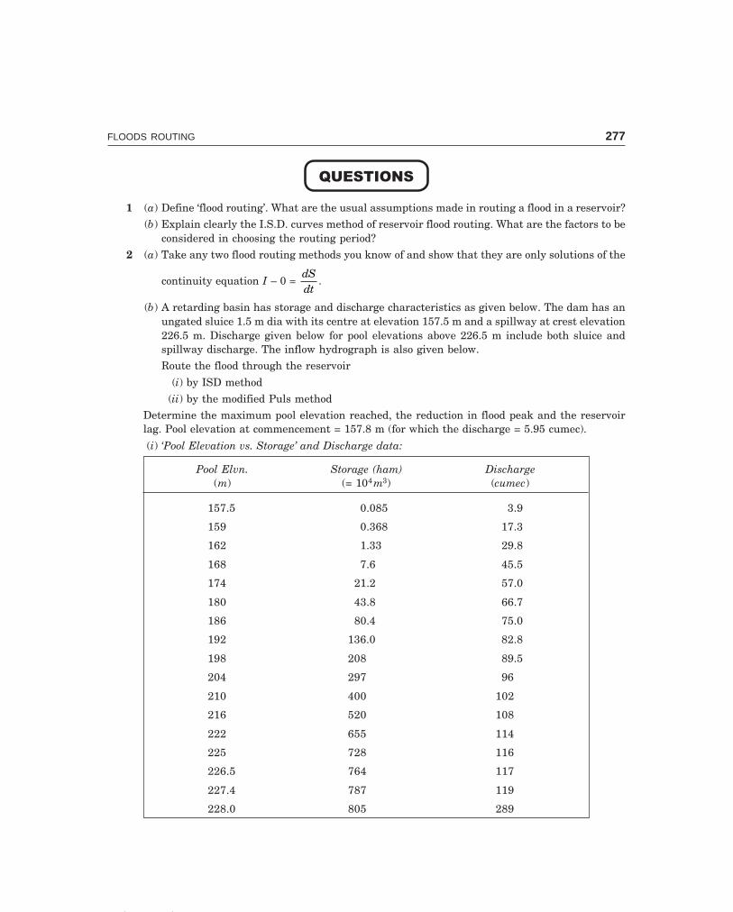
C-9\N-HYDRO\HYD9-1.PM5 277
FLOODS ROUTING 277
�������
1 (a) Define ‘flood routing’. What are the usual assumptions made in routing a flood in a reservoir?
(b) Explain clearly the I.S.D. curves method of reservoir flood routing. What are the factors to beconsidered in choosing the routing period?
2 (a) Take any two flood routing methods you know of and show that they are only solutions of the
continuity equation I – 0 = dSdt
.
(b) A retarding basin has storage and discharge characteristics as given below. The dam has anungated sluice 1.5 m dia with its centre at elevation 157.5 m and a spillway at crest elevation226.5 m. Discharge given below for pool elevations above 226.5 m include both sluice andspillway discharge. The inflow hydrograph is also given below.
Route the flood through the reservoir
(i) by ISD method
(ii) by the modified Puls method
Determine the maximum pool elevation reached, the reduction in flood peak and the reservoirlag. Pool elevation at commencement = 157.8 m (for which the discharge = 5.95 cumec).
(i) ‘Pool Elevation vs. Storage’ and Discharge data:
Pool Elvn. Storage (ham) Discharge(m) (= 104m3) (cumec)
157.5 0.085 3.9
159 0.368 17.3
162 1.33 29.8
168 7.6 45.5
174 21.2 57.0
180 43.8 66.7
186 80.4 75.0
192 136.0 82.8
198 208 89.5
204 297 96
210 400 102
216 520 108
222 655 114
225 728 116
226.5 764 117
227.4 787 119
228.0 805 289

C-9\N-HYDRO\HYD9-1.PM5 278
278 HYDROLOGY
(ii) Inflow hydrograph data
Time Inflow Time Inflow(hr) (cumec) (hr) (cumec)
0 15 36 141
6 57 42 93
12 159 48 60
18 258 54 33
24 246 60 18
30 198
(Hint Take routing period t = 6 hr = 1/4 day)
Draw the curves:
(i) Pool elevation vs. discharge (outflow)
(ii) Discharge (outflow) in comec vs. S ± Ot2
in cumec – 14 day, for ISD method of routing.
(iii) Discharge (outflow) in cumec vs. 2St
± O in cumec, for modified Puls method of routing.
3 (a) How does ‘stream flow routing’ differ from reservoir flood routing?
(b) The inflow hydrograph readings for a stream reach are given below for which the Muskingumcoefficients of K = 30 hr and x = 0.2 apply. Route the flood through the reach and determinethe reduction in peak and the time of peak of outflow. Outflow at the beginning of the floodmay be taken as the same as inflow.
Time Inflow Time Inflow(hr) (cumec) (hr) (cumec)
0 15 132 32
12 16 144 28
24 31 156 24
36 96 168 22
48 121 180 20
60 102 192 19
72 85 204 18
84 70 216 17
96 57 228 16
108 47 240 15
120 39

C-9\N-HYDRO\HYD9-1.PM5 279
FLOODS ROUTING 279
4 (a) Show that storage in a stream reach can be expressed in terms of inflow and outflow in theform:
S = K [xI + (1 – x) 0]
(b) The inflow and outflow hydrographs for a reach of a river are given below. Determine thebest values of the Muskingum coefficients K and x for the reach.
Time Inflow Outflow(hr) (cumec) (cumec)
0 20 20
12 191 30
24 249 120
36 164 176
48 110 164
60 82 135
72 62 116
84 48 90
96 32 68
108 28 52

Chapter 10
STORAGE, PONDAGE AND FLOW
DURATION CURVES
280
10.1 RESERVOIR MASS CURVE AND STORAGE
During high flows, water flowing in a river has to be stored so that a uniform supply of watercan be assured, for water resources utilisation like irrigation, water supply, power generation,etc. during periods of low flows of the river.
A mass diagram is a graphical representation of cumulative inflow into the reservoirversus time which may be monthly or yearly. A mass curve is shown in Fig. 10.1 for a 2-yearperiod. The slope of the mass curve at any point is a measure of the inflow rate at that time.Required rates of draw off from the reservoir are marked by drawing tangents, having slopesequal to the demand rates, at the highest points of the mass curve. The maximum departurebetween the demand line and the mass curve represents the storage capacity of the reservoirrequired to meet the demand. A demand line must intersect the mass curve when extendedforward, otherwise the reservoir is not going to refill. The vertical distance between the suc-cessive tangents represent the water wasted over the spillway. The salient features in themass curve of flow in Fig. 10.1 are:
a-b: inflow rate exceeds the demand rate of x cumec and reservoir is overflowingb: inflow rate equals demand rate and the reservoir is just full
b-c: inflow rate is less than the demand rate and the water is drawn from storagec: inflow rate equals demand rate and S1 is the draw off from the reservoir (Mm3)
c-d: inflow rate exceeds demand rate and the reservoir is fillingd: reservoir is full again
d-e: same as a-be: similar to b
e-f: similar to b-cf: inflow rate equals demand rate and S2 is the draw off from the reservoir
f-g: similar to c-dTo meet the demand rate of x cumec the departure S2 > S1; hence, the storage capacity
of the reservoir is S2 Mm3. If the storage capacity of the reservoir, from economic considera-tions, is kept as S1 Mm3, the demand rate of x cumec can not be maintained during the timee-f and it can be at a lesser rate of y cumec (y < x).

C-9\N-HYDRO\HYD10-1.PM5 281
STORAGE, PONDAGE AND FLOW DURATION CURVES 281
Res.emptyf
For the demand rateof x cumec, S > S2 1
Storage capacity
of reservoir = S Mm23
Water wastedover spillway
x cumec
Water drawnfrom storage
e
d
Reservoirfills again
x cumec
Reservoirfull
Reg.empty
Water drawnfrom storage
Mass curveof inflow
b
Draw offrate
Slope =x - cu
mec
=y - cumec
1 year1 year
Cum.storageper year
Cum.storageper year
Inflow rate into reservoirDraw off rate
1400
1300
1200
1100
1000
900
800
700
600
500
400
300
200
100
Cum
ulat
ive
inflo
w, (
M.m
orha
-m
)3
0 aA S O N D J F M A M J J A S O N D J F M A M J J A S
19701970 19711971 19721972
Time (months & year)
y cumec
S1S1
g
c
S2S1
s1s1
S2S2
Fig. 10.1 Storage capacity of reservoir from mass curve
The use of mass curve is to determine:(i) the storage capacity of the reservoir required to meet a particular withdrawal rate.
(ii) the possible rate of withdrawal from a reservoir of specified storage capacity.The observed inflow rates have to be adjusted for the monthly evaporation from the
reservoir surface, precipitation, seepage through the dam, inflow from adjacent basins, re-quired releases for downstream users, sediment inflow, etc. while calculating the storage ca-pacity of the reservoir.
The average flow figures for the site of a proposed dam are collected for about 10 years.From this record the flow figures for the driest year are used for drawing the mass flow curve.Graphical analysis is enough for preliminary studies. Final studies are made by tabular com-putation. If tangents are drawn to the crest and trough of the mass curve such that the depar-ture of the lines represents the specified reservoir capacity, the slope of the tangent at thecrest gives the continuous flow that can be maintained with the available storage capacity.From this the greatest continuous power output for the available fall at the site for a givenplant efficiency and load factor can be determined.
From the daily flow data a hydrograph or a bar graph is drawn for the maximum floodduring the period of 10 years and the spillway capacity to pass this flood with the availablestorage capacity is determined. Thus, the power and the flood control potentialities of the siteare investigated. Also see Appendix-C.

C-9\N-HYDRO\HYD10-1.PM5 282
282 HYDROLOGY
The mass curve of water utilisation need not be a straight line. The dashed curve inFig. 10.2 shows the cumulative requirements of water use in different months as comparedwith monthly cumulatively inflow. The maximum draft in the reservoir (i.e., maximum depar-ture of the water use and inflow curves) occurs by the end of April. The reservoir again be-comes full by the end of September when the two curves intersect.
Max draftin May
Max draftin May
Reservoir fullby end of Sept.
Mass curve of waterutilisation
Reservoirfull onDec. 1
Reservoirfull onDec. 1
Mass curve ofmonthly inflow
1
2
700
600
500
400
300
200
100
0D J F M A M J J A S O N D
Time (months)
Cum
ulat
ive
inflo
w
(M.m
orha
m)
3
Fig. 10.2 Mass curves of water utilisation and monthly inflow
Example 10.1 The following is a record of the mean monthly discharges of a river in a dryyear. The available fall is 80 m. Determine
(i) the minimum capacity of a reservoir if the entire annual inflow is to be drawn off ata uniform rate (with no flow going into waste over the spillway).
(ii) the amount of water which must be initially stored to maintain the uniform draw off.(iii) the uniform power output assuming a plant efficiency of 70%.
(iv) If the amount of water initially stored is 125 Mm3, the maximum possible draw offrate and the amount of water wasted over the spillway (assuming the same reservoir capacitydetermined in (i) above.
(v) if the largest reservoir that can be economically constructed is of capacity 125 Mm3,the maximum possible output and the amount of water wasted over the spillway.
(vi) the capacity of the reservoir to produce 22.5 megawatts continuously throughout theyear.
Month Mean flow Month Mean flow(cumec) (cumec)
Jan. 29.7 July 68.0
Feb. 75.3 Aug. 50.2
March 66.8 Sept. 74.5
April 57.2 Oct. 66.8
May 23.2 Nov. 40.5
June 26.3 Dec. 26.3
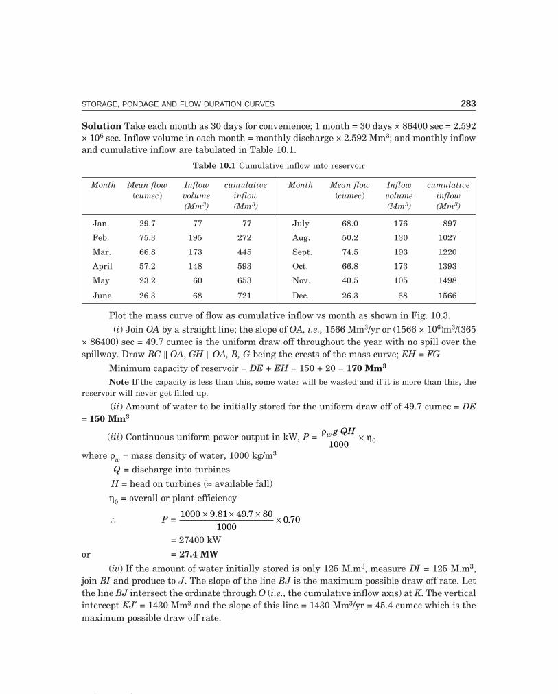
C-9\N-HYDRO\HYD10-1.PM5 283
STORAGE, PONDAGE AND FLOW DURATION CURVES 283
Solution Take each month as 30 days for convenience; 1 month = 30 days × 86400 sec = 2.592× 10⁶ sec. Inflow volume in each month = monthly discharge × 2.592 Mm3; and monthly inflowand cumulative inflow are tabulated in Table 10.1.
Table 10.1 Cumulative inflow into reservoir
Month Mean flow Inflow cumulative Month Mean flow Inflow cumulative(cumec) volume inflow (cumec) volume inflow
(Mm3) (Mm3) (Mm3) (Mm3)
Jan. 29.7 77 77 July 68.0 176 897
Feb. 75.3 195 272 Aug. 50.2 130 1027
Mar. 66.8 173 445 Sept. 74.5 193 1220
April 57.2 148 593 Oct. 66.8 173 1393
May 23.2 60 653 Nov. 40.5 105 1498
June 26.3 68 721 Dec. 26.3 68 1566
Plot the mass curve of flow as cumulative inflow vs month as shown in Fig. 10.3.
(i) Join OA by a straight line; the slope of OA, i.e., 1566 Mm3/yr or (1566 × 106)m3/(365× 86400) sec = 49.7 cumec is the uniform draw off throughout the year with no spill over thespillway. Draw BC || OA, GH || OA, B, G being the crests of the mass curve; EH = FG
Minimum capacity of reservoir = DE + EH = 150 + 20 = 170 Mm3
Note If the capacity is less than this, some water will be wasted and if it is more than this, thereservoir will never get filled up.
(ii) Amount of water to be initially stored for the uniform draw off of 49.7 cumec = DE= 150 Mm3
(iii) Continuous uniform power output in kW, P = ρ
ηw g QH1000 0×
where ρw = mass density of water, 1000 kg/m3
Q = discharge into turbines
H = head on turbines (≈ available fall)
η0 = overall or plant efficiency
∴ P = 1000 49 7 801000
0 70× × × ×9.81 .
.
= 27400 kW
or = 27.4 MW
(iv) If the amount of water initially stored is only 125 M.m3, measure DI = 125 M.m3,join BI and produce to J. The slope of the line BJ is the maximum possible draw off rate. Letthe line BJ intersect the ordinate through O (i.e., the cumulative inflow axis) at K. The verticalintercept KJ′ = 1430 Mm3 and the slope of this line = 1430 Mm3/yr = 45.4 cumec which is themaximum possible draw off rate.

C-9\N-HYDRO\HYD10-1.PM5 284
284 HYDROLOGY
Spilling(during MN,RU)
Spilling(during MN,RU)
Spillage = PM, RS SPP
G N
CM
L
T
FH V
UU
(170)
(150)E
I125
I125
B
K
DD
A (1566
M.m )3
100z
100z
(1287 Mm )3
Q
J¢ J
Cum
ulat
ive
inflo
w, M
.m3
KJ
=14
30M
.m¢
3
1 - year base
Line - slope = M.m /yr cumec MW3
OA // BC // GH = 1566 = 49.7 27.4KJ // HL // GT = 1430 = 45.4 25.0BV // OQ = 1287 = 40.8 22.5
J¢ kJ¢ = 1430 M.m31600
1500
1400
1300
1200
1100
1000
900
800
700
600
500
400
300
200
100
0J F M A M J J A S O N D
Time (months)
Cum
ulat
ive
inflo
w(M
m3 )
49.7 cumec45.4 cumec
40.8 cumecDraw off rates
A
QR
1566 Mm3
1430 Mm3
1287 Mm3
O1 yearTime
b. Key for slopes (Q)
Cumulativestorage
C. Mass curve analysis
Mass curve ofreservoir inflow
Reservoir full
B
Draw off rates
a. key for mass curve
170 M.m3150 M.m
3
20 M.m3D
H
z
E
125 M.m3
100 M.m3D
C
N
G
F
P40 Mm
3
M
R
VT
85 Mm3
Spillage
A
Q
1560Mm
3
1287Mm
3
Q P
K
L j
O
I
R
Fig. 10.3 Mass curve studies in reservoir design (Example 10.1)
To maintain the same reservoir capacity of 170 M.m3, draw the straight line HL || KJintersecting the mass curve of flow at M and N. Draw the straight line GT || HL. The verticalintercept PM gives the amount of water wasted over the spillway (during the time period MN)which is 40 Mm3.
(v) If the reservoir capacity is limited to 125 M.m3 from economic considerations, theline KJ intersects the mass curve of flow at R. Let the vertical at R meet the line GT (GT || KJ)at S. In this case the amount of water wasted over the spillway = RS = 85 Mm3. The maximumpossible output in this case for a uniform draw off rate of 45.4 cumec is
P′ = 27.4 × 45 449 7
.
. = 25 MW

C-9\N-HYDRO\HYD10-1.PM5 285
STORAGE, PONDAGE AND FLOW DURATION CURVES 285
(vi) For a continuous power output of 22.5 MW the uniform draw off rate can be deter-mined from the equation
22500 kW = 1000 9 81 80
1000× × ×. Q
× 0.70
Q = 40.8 cumec
which can also be calculated as 49.7 × 22 527 4
.
. = 40.8 cumec = 40.8 (365 × 86400 sec) = 1287 Mm3/yr.
On the 1-year base, draw the ordinate at the end of December = 1287 M.m3 and join the lineOQ (dashed line). The slope of this line gives the required draw off rate (40.8 cumec) to producea uniform power output of 22.5 mW. Through B and D, i.e., the crest and the trough drawtangents parallel to the dashed line OQ (BV || OQ). The vertical intercept between the twotangents DZ gives the required capacity of the reservoir as 100 Mm3.
10.2 FLOW DURATION CURVES
Flow duration curves show the percentage of time that certain values of discharge weekly,monthly or yearly were equalled or exceeded in the available number of years of record. Theselection of the time interval depends on the purpose of the study. As the time interval in-creases the range of the curve decreases, Fig. 10.4. While daily flow rates of small storms areuseful for the pondage studies in a runoff river power development plant, monthly flow ratesfor a number of years are useful in power development plants from a large storage reservoir.The flow duration curve is actually a river discharge frequency curve and longer the period ofrecord, more accurate is the indication of the long term yield of a stream. A flat curve indicatesa river with a few floods with large ground water contribution, while a steep curve indicatesfrequent floods and dry periods with little ground water contribution. Since the area under thecurve represents the volume of flow, the storage will affect the flow duration curve as shownby the dashed line in Fig. 10.5; i.e., reducing the extreme flows and increasing the very lowflows.
Mean daily flows
Mean monthly flows
Mean annual flows
Flo
wra
teQ
(cum
ec)
600
500
400
300
200
100
00 20 40 60 80 100
% time Q=>
Fig. 10.4 Flow duration curves—effect of observation period

C-9\N-HYDRO\HYD10-1.PM5 286
286 HYDROLOGY
Flow duration curve(monthly flows)
Storage effect onflow duration curve
Flow duration curve
(Weekly flows)
Flow duration curve
(Weekly flows)
Power duration curve
335
272
600
500
400
300
200
100
00 10 20 30 40 50 60 70 8075 90 100
0
50
100
150
200
250
300
Mea
nm
onth
lyflo
wQ
(cum
ec)
Pow
erP,
MW
% time > Q or P values indicated
157
Fig. 10.5 Flow duration and power duration curves (Example 10.2)
Since drought is often defined in terms of a fixed period of time with less than someminimum amount of rainfall, the flow duration curves are useful for determining the durationof floods or droughts, the latter being of prime importance in the semi-arid regions. Durationcurves for long periods of runoff are also useful for deciding the flow rates to be used forparticular purposes, say, for power development.
The usual procedure is to arrange the flow values (or range of flow values weekly, monthlyor yearly) in the available period of record (usually a minimum of 10 years) in the ascendingorder of magnitude and the number of occurrences of each flow value (or range of flow values).From this the number of times and the percent of time each flow value (or range of flow values)has been equalled or exceeded in the period of record may be obtained. The duration curve isconstructed by plotting each flow value (or lower value of the class interval) against the per-cent of time it has been equalled or exceeded. The power duration curve is the same as the flowduration curve, the discharge scale being converted to power units corresponding to the avail-able head (assuming the head constant) since
Power in kW, P = ρ
ηw g QH1000 0×
or, P = a constant × Qwhere Q is the flow value being equalled or exceeded during a certain percent of time.
Flow duration curves are useful in the studies relating to navigation problems, waterpower, water supply, irrigation and sanitation.Example 10.2 The following data are obtained from the records of the mean monthly flows ofa river for 10 years. The head available at the site of the power plant is 60 m and the plantefficiency is 80%.

C-9\N-HYDRO\HYD10-1.PM5 287
STORAGE, PONDAGE AND FLOW DURATION CURVES 287
→
→
Mean monthly flow range No. of occurrences(cumec) (in 10-yr period)
100-149 3150-199 4200-249 16250-299 21300-349 24350-399 21400-499 20450-499 9500-549 2
(a) Plot(i) The flow duration curve (ii) The power duration curve
(b) Determine the mean monthly flow that can be expected and the average power thatcan be developed.
(c) Indicate the effect of storage on the flow duration curve obtained.(d) What would be the trend of the curve if the mean weekly flow data are used instead of
monthly flows.Solution (a) The mean monthly flow ranges are arranged in the ascending order as shown inTable 10.2. The number of times that each mean monthly flow range (class interval, C.I.) hasbeen equalled or exceeded (m) is worked out as cumulative number of occurrences startingfrom the bottom of the column of number of occurrences, since the C.I. of the monthly flows,are arranged in the ascending order of magnitude. It should be noted that the flow values arearranged in the ascending order of magnitude in the flow duration analysis, since the minimum
Table 10.2 Flow duration analysis of mean monthly flow data of ariver in a 10 yr period (Example 10.2)
Mean monthly No. of No. of time Percent of time Monthly powerflow occurrences equalled or lower value of P = 0.472 Q
class interval (in 10-yr exceeded CI equalled or (MW)C.I. period) (m) exceeded Q = lower value of
(cumec) = mn
× 100% C.I.
100-149 3 120 100 47.2150-199 4 117 97.5 70.8200-249 16 113 94.2 94.4250-299 21 97 80.8 118300-349 24 76 63.3 142350-399 21 52 43.3 165400-499 20 → 31 25.8 189450-499 9 + → 11 9.2 212500-549 2 + → 2 1.7 236
Total n = 120
Note: For drought–duration studies, m = No. of times equal to or less than the flow value and
has to be worked from the top; percent of time ≤ the flow value is mn
× 100. In this example, m = 3, 7, 23,
44, ... and % of time ≤ Q are 2.5, 5.83, 19.2, 36.7. ...., respectively (from top).

C-9\N-HYDRO\HYD10-1.PM5 288
288 HYDROLOGY
continuous flow that can be expected almost throughout the year (i.e., for a major percent oftime) is required particularly in drought duration and power duration studies, while in floodflow analysis the CI may be arranged in the descending order of magnitude and m is workedout from the top as cumulative number of occurrences since the high flows are of interest. Thepercent of time that each CI is equalled or exceeded is worked out as the percent of the totalnumber of occurrences (m) of the particular CI out of the 120 (= 10 yr × 12 = n) mean monthly
flow values, i.e., = mn
× 100. The monthly power developed in megawatts,
P = gQH1000
× η0 = 9.81
0.80× ×F
HGIKJ
601000
Q
P = 0.472 Qwhere Q is the lower value of the CI Thus, for each value of Q, P can be calculated.
(i) The flow duration curve is obtained by plotting Q vs. percent of time, Fig. 10.5,(Q = lower value of the CI).
(ii) The power duration curve is obtained by plotting P vs. percent of time, Fig. 10.5.(b) The mean monthly flow that can be expected is the flow that is available for 50% of
the time i.e., 357.5 cumec from the flow duration curve drawn. The average power that can bedeveloped i.e., from the flow available for 50% of the time, is 167 MW, from the power durationcurve drawn.
(c) The effect of storage is to raise the flow duration curve on the dry weather portionand lower it on the high flow portion and thus tends to equalise the flow at different times ofthe year, as indicated in Fig. 10.5.
(d) If the mean weekly flow data are used instead of the monthly flow data, the flowduration curve lies below the curve obtained from monthly flows for about 75% of the timetowards the drier part of the year and above it for the rest of the year as indicated in Fig. 10.5.
In fact the flow duration curve obtained from daily flow data gives the details moreaccurately (particularly near the ends) than the curves obtained from weekly or monthly flowdata but the latter provide smooth curves because of their averaged out values. What durationis to be used depends upon the purpose for which the flow duration curve is intended.
10.3 PONDAGE
While storage refers to large reservoirs to take care of monthly or seasonal fluctuations in theriver flow, pondage usually refers to the small storage at the back of a weir, in run-of-riverplants, for temporarily storing water during non-working hours, idle days and low load peri-ods for use during hours of peak load demand. Run-of-river plants are feasible for streamswhich have a minimum dry weather flow or receive flow as regulated by any storage reservoirupstream.
Pondage factor is the ratio of the total inflow hours in a week to the total number ofhours of working of the power plant in that week. For example, assuming constant streamflow, if a power plant operates for 6 days in a week at 8 hours per day, then the pondage factor
would be 7 246 8×× = 3.5, and if the plant works only for 5 days in a week, the pondage factor

C-9\N-HYDRO\HYD10-1.PM5 289
STORAGE, PONDAGE AND FLOW DURATION CURVES 289
would be 7 245 8××
= 4.2 and the pondage required in the latter case would be 48 16
24+
× daily
flow volume = 83
of daily flow-volume.Thus the pondage factor serves as a rough guide of the
amount of pondage required when the stream flow is constant and the plant works only for apart of the period. Pondage is needed to cover the following four aspects:
(i) To store the idle day flow.(ii) For use during hours of peak load.
(iii) To balance the fluctuations in the stream flow.(iv) To compensate for wastage (due to leakage) and spillage.
Example 10.3 The available flow for 97% of the time (i.e., in a year) in a river is 30 cumec. Arun-of-river plant is proposed on this river to operate for 6 days in a week round the clock. Theplant supplies power to a variable load whose variation is given below:
Period (hr) 0–6 6–12 12–18 18–24
Load during period24 hr average load-
ratio 0.6 1.4 1.5 0.5
The other relevant data are given below:
Head at full pond level = 16 mMaximum allowable fluctuation of pond level = 1 m
Plant efficiency = 80%Pondage to cover inflow fluctuations = 20% of average daily flow
Pondage to cover wastage and spillage = 10%Determine:
(i) the average load that can be developed(ii) daily load factor
(iii) plant capacity(iv) weekly energy output
(v) pondage required and the surface area of the pond for satisfactory operationSolution (i) 7 days flow has to be used in 6 days
∴ Average flow available for power development
Q = 30 × 76 = 35 cumec
Since maximum allowable fluctuation of pond level is 1 m, average head
H = 16 15
2+
= 15.5 m
The average load that can be developed
P = gQH1000
× η0
= 9.81 35 15.5
1000× ×
× 0.8 = 4.27 MW

C-9\N-HYDRO\HYD10-1.PM5 290
290 HYDROLOGY
(ii) Daily load factor = average load
peak load =
11.5
= 0.67
(iii) Plant capacity = 4.27 × 1.5 = 6.4 MW(iv) Weekly energy output = Average load in kW × No. of working hours
= (4.27 × 1000)(6 × 24) = 6.15 × 10⁵ kWhIt should be noted that the installed capacity has to be equal to the peak load and the
number of units (kWh) generated will be governed by the average load.(v) Pondage required
(a) to store the idle day’s flow = 30 × 86400 = 2.592 × 10⁶ m3, or 2.592 Mm3
(b) to store the excess flow during low loads to meet the peak load demand. Since powerdeveloped is proportional to discharge (assuming constant average head of 15.5 m), flow re-quired during peak load periods of 6.00 to 12.00 hr is (1.4 – 1) 35 cumec and from 12.00 to 18.00hr is (1.5 – 1) 35 cumec.
∴ pondage to meet peak load demand= (0.4 + 0.5) 35 cumec for 6 hr= (0.9 × 35)(6 × 60 × 60)= 6.81 × 10⁵ m3, or 0.681 Mm3
(c) pondage to cover inflow fluctuations= (0.20 × 30) 86400= 5.18 × 10⁵ m3, or 0.518 Mm3
Total of (a), (b) and (c) = 3.791 Mm3
Add 10% for wastage and spillage = 0.379 Mm3
Total pondage required = 4.170 Mm3
Since the maximum fluctuation of pond level is 1 mthe surface area of pond = 4.170 × 10⁶ m2
or 4.17 km2, or 417 haExample 10.4 A run-of-river hydroelectric plant with an effective head of 22 m and
plant efficiency of 80% supplies power to a variable load as given below:
Time (hr) Load (1000 kW) Time (hr) Load (1000 kW)
MN 0-2 11.4 12-14 44.2
2-4 5.6 14-16 44.4
4-6 25.6 16-18 74.2
6-8 53.2 18-20 37.8
8-10 44.8 20-22 30.0
N 10-12 39.4 22-24 18.0
Draw the load curve and determine:
(i) the minimum average daily flow to supply the indicated load.(ii) pondage required to produce the necessary power at the peak.
(iii) the plant load factor.

C-9\N-HYDRO\HYD10-1.PM5 291
STORAGE, PONDAGE AND FLOW DURATION CURVES 291
Solution (i) The load curve is shown in Fig. 10.6.
35.72 (1000) kw
Ave. load
Time (hr)
0 2 4 6 8 10 12 14 16 18 20 22 24
Load factor = 35.7274.2
= 0.482or 48.2%
Peak load74.2 (1000) kW80
70
60
50
40
30
20
10
Load
(100
0kW
)
0
Fig. 10.6 Daily load curve (Example 10.4)
Total of loads at 2 hr intervals = 428.6 kW
Average load = 428.6 1000 kW 2hr
24 hr× ×
= 35.72 × 1000 kW
Flow (Q) required to develop the average load1000 22
1000× × ×9.81 Q
× 0.8 = 35.72 × 1000
∴ Q = 207 cumec(ii) Flow required to produce the required load demand
Q = 207
35 72. × Load in 1000 kW
∴ Q = 5.8 × Load in 1000 kWTo determine the pondage capacity the following table is prepared:
Time Load Required Deviation from the average(hr) (1000 kW) flow flow of 207 cumec
P (cumec) Deficiency Excess5.8 P (cumec) (cumec)
MN: 0-2 11.4 66.10 140.90
2-4 5.6 32.46 174.54
4-6 25.6 148.40 58.60
6-8 53.2 308.20 101.20
8-10 44.8 260.00 53.00
N: 10-12 39.4 228.50 21.50
12-14 44.2 256.00 49.00
14-16 44.4 257.40 50.40(Contd.)...page 292

C-9\N-HYDRO\HYD10-1.PM5 292
292 HYDROLOGY
16-18 74.2 430.00 223.00
18-20 37.8 219.40 12.40
20-22 30.0 174.00 33.00
22-24 18.0 104.30 102.70
Total: 428.6 510.50 509.74
From the above table Total deficiency = total excess = 510 cumec
∴ Pondage capacity required = 510 cumec for 2 hr = 510 (2 × 60 × 60) = 3.67 Mm3
(iii) Plant Load factor = average load
peak load
L.F. = 35 7274 20
.
. = 0.482 or 48.2%.
������
I Choose the correct statement/s in the following:1 From a reservoir mass curve the following information may be obtained:
(i) the storage capacity required for a uniform discharge and power output.(ii) the maximum discharge possible and power output for a specified storage capacity.
(iii) the month when the reservoir is empty or just fall.(iv) the months during which water is overflowing over the spillway.(v) the reservoir pool elevation at any time.
(vi) all the above.2 A flow duration curve indicates
(i) the stream flow available for different percent of time(ii) the firm power (iii) the duration of floods or droughts(iv) the effect of storage (v) the power available for different percent of time(vi) all the above times.
3 Pondage is required across a river(i) which becomes dry in summer
(ii) which gets occasional releases from an upstream reservoir(iii) which has a sustained dry weather flow(iv) to take care of seasonal fluctuations of streamflow(v) to store water during off-hours, idle day and low load periods, for use during hours of peak load
(vi) to compensate for the losses due to evaporation, leakage and spillage(vii) for all the above cases. (1. vi; 2. vi; 3. iii, iv, v, vi)
II Match the items in ‘A’ with items in ‘B’A B
(i) Storage (a) 97% of time on power-duration curve(ii) Pondage (b) Arid region
(iii) Minimum hydrorate (c) Run-of-river plant
(iv) Drought-duration (d) Reservoir mass curve

C-9\N-HYDRO\HYD10-1.PM5 293
STORAGE, PONDAGE AND FLOW DURATION CURVES 293
III Say ‘true’ or ‘false’; if false, give the correct statement:
(i) A mass curve is a graphical representation of cumulative inflow into the reservoir versustime.
(ii) The vertical distance between the successive tangents to the mass curve peaks (the slopes ofthe tangents = demand rates) represents the storage capacity of the reservoir.
(iii) The slope of the mass curve at any point gives the inflow rate at that time into the reservoir.(iv) The draw-off rates are marked by drawing tangents at the peaks, having slopes equal to the
demand rates.(v) The maximum departure between the demand line and the mass curve gives the water wasted
over the spillway.(vi) A demand line must intersect the mass curve when extended forward, otherwise the reser-
voir is not going to refill.(vii) The maximum departure of the mass curve of water use and mass curve of inflow indicates
the month of maximum draft in the reservoir.(viii) The weekly flow duration curve lies above that of the monthly flow for about 75% of the time
(towards the drier part of the year) and below it for the rest of the year.(ix) Though the daily flow duration curve gives the details more accurately (particularly near the
ends), the weekly or monthly flow duration curves plot smooth curves (because of their aver-aged out values).
(x) Larger the period of record, more accurate and flatter is the flow duration curve.(xi) The effect of storage is to lower the flow duration curve on the dry weather portion and raise
it on the high flow portion, thus depicting marked variation in the flow at different times ofthe year.
(xii) The pondage factor for a constant river discharge into a pond with 8-hour plant operation perday for 6 days in a weak is 3.5, neglecting Sunday (idle-day) and the pondage required is 5/3of the daily-flow volume.
(xiii) Run-of-river plants are feasible for streams, which do not have a sustained dry weather flowor receive flow releases occasionally as regulated by an upstream reservoir.
(xiv) The flow-duration curves are useful for drought-duration studies particularly in semi-aridregions. (false: ii, v, vii, x, xi, xii)
�������
1 (a) Sketch a mass curve of run-off and explain how it is helpful in determining:
(a) the storage required to satisfy a given constant demand.
(b) the safe yield available from a given storage.
(b) The estimated monthly flow in a river is as follows:
Month Flow Month Flow(Mm3) (Mm3)
Jan. 7.6 July 10.7
Feb. 19.5 Aug. 13.0
March 17.3 Sept. 19.2
April 10.5 Oct. 17.2
May 5.9 Nov. 10.5
June 6.8 Dec. 6.8

C-9\N-HYDRO\HYD10-1.PM5 294
294 HYDROLOGY
The available fall is 42 m. What size of reservoir will be necessary to give the greatest continu-ous uniform output and what will be this power if the plant efficiency is 70%. If the largestreservoir, which can be economically constructed has a capacity of 8.8 Mm3, what will be thenthe greatest output?
2 (a) Give the method of finding out the size of reservoir using stream flow records and demand.
(b) The following is a record of mean monthly discharges of a river in a dry year:
Month Mean flow Month Mean flow(cumec) (cumec)
April 56.6 Oct. 161.5
May 62.2 Nov. 133.0
June 119.0 Dec. 190.0
July 258.0 Jan. 212.3
Aug. 234.0 Feb. 184.0
Sept. 201.5 March 127.5
The average net head available is 30.5 m and the average efficiency of a hydro-electric plant maybe taken as 85%. Estimate the storage required to produce a firm power of 40 MW and themaximum firm power available.
3 The monthly inflow into a reservoir is as follows:
Month Flow Month Flow(Mm3) (Mm3)
Jan. 340 July 400
Feb. 360 Aug. 300
March 300 Sept. 310
April 270 Oct. 330
May 240 Nov. 350
June 290 Dec. 320
The water turbines have an output of 22.5 MW working under a net head of 24 m and overallefficiency of 80%.
Determine the minimum capacity of the reservoir to satisfy the uniform demand for water andthe total quantity of water wasted during the year assuming that at the beginning of January,the reservoir is full.
4 The quantity of water flowing in a river during each successive month is given below in Mm3.
4.2, 5.1, 8.5, 27.5, 45.3, 30.6, 14.2, 11.1, 10.2, 9.3, 8.8.
Determine the minimum capacity of a reservoir, if the above water is to be drawn off at a uni-form rate and there should be no loss by flow over the spillway.
Also estimate the amount of water, which must be initially stored to maintain the uniform drawoff.
Also calculate the electrical energy that could be generated per year, if the average availablehead is 36.5 m and the plant efficiency is 80%.
5 The following is a record of the power demand and of the streamflow taken in a day, for every2-hr intervals (the record gives the average for the two hour periods).
C-9\N-HYDRO\HYD10-1.PM5 295
STORAGE, PONDAGE AND FLOW DURATION CURVES 295
Time Power demand Stream flow(hr) (1000 kW) (cumec)
MN: 0-2 11.4 59.5
2-4 5.6 57.4
4-6 25.6 55.2
6-8 53.2 53.8
8-10 44.8 52.4
N: 10-12 39.4 51.0
12-14 44.2 49.6
14-16 44.4 51.0
16-18 74.2 52.4
18-20 37.8 53.8
20-22 30.0 55.2
22-24 18.0 56.6
The average net head available is 109.3 m. The average plant efficiency is 85%. Determine thenecessary storage, if the demand is to be just met.
6 Explain the significance of the terms; flow-duration curves, mass curves, pondage and storage.State the limiting conditions for economic storage and utilization of water resources in a countrywhere the majority of rivers are not perennial?
Sketch one in which the power potential can be augmented further downstream.
7 Construct a mass curve from the following data of flow for a given site.
Weeks Weekly flow(cumec)
1-6 600
7-12 700
13-18 300
19-24 400
25-30 1700
31-36 1300
37-42 900
43-48 600
49-52 300
Estimate the size of reservoir and the possible maximum rate of flow that could be availablefrom it. (5500 Mm3, 773 cumec)

C-9\N-HYDRO\HYD10-1.PM5 296
296 HYDROLOGY
8 The average weekly discharge as measured at a given site is as follows:
Week Flow Week Flow(cumec) (cumec)
1 1000 14 1200
2 900 15 1000
3 909 16 900
4 800 17 800
5 800 18 500
6 600 19 400
7 500 20 400
8 500 21 300
9 800 22 300
10 800 23 400
11 1000 24 400
12 1100 25 500
13 1100 26 500
Plot
(a) the hydrograph of weekly flow.
(b) the flow-duration curve.
(c) the power-duration curve if the head available is 50 m and the efficiency of the turbine-generator set is 85%.
Determine the power that can be developed per cumec, the maximum power, average power, andtotal energy produced during 26 weeks. (417 kW, 485 MW, 300 MW, 1.31 GWh)
9 Average daily flows in a river in typical low water week are given below. A run-of-river plant isproposed on this river to operate for 6 days in a week round the clock. The full pond effectivehead on turbines is 20 m and the plant efficiency is 80%. Maximum allowable fluctuation of pondlevel is 1 m.
Determine
(i) the capacity of the pond required to give a maximum uniform output.
(ii) the surface area of pond for satisfactory operation.
(iii) the weekly energy output (KWH) from the plant.
Day: Sun. Mon. Tues. Wed. Thurs. Fri. Sat.
Flow (cumec): 26 35 40 50 45 40 30
10 Typical weekly and daily releases of water from an upstream reservoir on a river are givenbelow. Estimate the pondage capacity to operate a run-of-river plant at downstream location sothat a steady uniform power output is available from the plant.
Weekly release pattern
Day: Sun. Mon. Tues. Wed. Thurs. Fri. Sat.
Flow: 25 30 40 50 40 35 25
release (cumec)

C-9\N-HYDRO\HYD10-1.PM5 297
STORAGE, PONDAGE AND FLOW DURATION CURVES 297
Daily release pattern
Time (hr): 0-6 6-12 12-18 18-24
% of ave. daily flow volume: 5 35 50 10
(Hint Pondage reqd. = weekly fluctuations + daily fluctuations)
11 During a low water week, the average daily flow in a river is 30 cumec and the pondage requiredfor the daily fluctuation is about 20% of the average daily flow. A run-of-river plant to be locatedon the river is to operate 6 days a week, round the clock and is connected to a variable load witha daily load factor of 50%. The pondage required for the daily load fluctuation may be taken asabout one-fifth of the mean flow to the turbine.
If the effective head on the turbine when the pond is full is 20 m and the maximum allowablefluctuation in pond level is 1 m, determine
(i) the capacity of the pond and its surface area.
(ii) the weekly energy output (KWH).
Assume a plant efficiency of 80%.

Chapter 11
11.1 SEDIMENT MOVEMENT AND DEPOSITION
As the silt originates from the water shed, the characteristics of the catchment such itsareal extent, soil types, land slopes, vegetal cover and climatic conditions like temperature,nature and intensity of rainfall, have a great significance in the sediment production in theform of sheet erosion, gully erosion and stream, channel erosion. In regions of moderate rain-fall, sheet erosion is the dominant source of total sediment load while in arid and semi-aridregions, gullying and stream-channel erosion furnish the greater part of the load.
Experiments have shown that the erosive power of water, flowing with a velocity V,varies as V 2 while the transporting ability of water varies as V 6. Sediment moves in thestream as suspended load (fine particles) in the flowing water, and as bed load (large parti-cles), which slides or rolls along the channel bottom. Sometimes, the particles (small particlesof sand and gravel) move by bouncing along the bed, which is termed as ‘saltation’, which is atransitional stage between bed and suspended load. The material, which moves as bed load atone section may be in suspension at another section.
The suspended sediment load of streams is measured by sampling the water, filtering toremove the sediment, drying and weighing the filtered material.
Sediment load, (ppm) = weight of sediment in the sample
weight of sediment laden water sample × 106
The samplers may be of ‘depth-integrating type’ or ‘point samplers’. Point samplers areused only where it is not possible to use the depth integrating type because of great depth ofhigh velocity, or for studies of sediment distribution in streams. The sample is usually col-lected in ‘pint bottle’ held in a sample of stream-lined body so as not to disturb the flow whilecollecting a representative sample.
The relation between the suspended-sediment transport Qs and stream flow Q is givenby
Qs = KQn ...(11.1)∴ log Qs = log K + n log Q ...(11.1 a)
and is often represented by a logarithmic plot of Qs vs. Q (Fig. 11.1); Qs = K when Q = 1, and nis the slope of the straight line plot and ≈ 2 to 3.
The sediment rating curve from a continuous record of stream flow provides a roughestimate of sediment inflow to reservoirs and the total sediment transport may be estimatedby adding 10-20% to the suspended sediment transport to allow for the bed load contribution.
RESERVOIR SEDIMENTATION
298
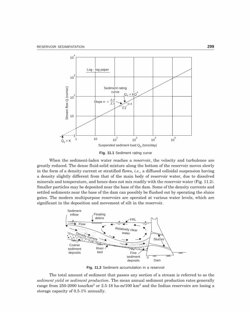
C-9\N-HYDRO\HYD11-1.PM5 299
RESERVOIR SEDIMENTATION 299
Q = Ks
111 10 10
210
310
410
5
Suspended sediment load Q (tons/day)S
Sediment ratingcurve
Sediment ratingcurve
Q = KQSn
Q = KQSn
Slope n =Slope n =ÑÑÑÑ ÑÑ
yyÑÑ xx
Log - log paperLog - log paper
104
103
102
10
Str
eam
flow
Q(c
umec
)
yxyx
Fig. 11.1 Sediment rating curve
When the sediment-laden water reaches a reservoir, the velocity and turbulence aregreatly reduced. The dense fluid-solid mixture along the bottom of the reservoir moves slowlyin the form of a density current or stratified flows, i.e., a diffused colloidal suspension havinga density slightly different from that of the main body of reservoir water, due to dissolvedminerals and temperature, and hence does not mix readily with the reservoir water (Fig. 11.2).Smaller particles may be deposited near the base of the dam. Some of the density currents andsettled sediments near the base of the dam can possibly be flushed out by operating the sluicegates. The modern multipurpose reservoirs are operated at various water levels, which aresignificant in the deposition and movement of silt in the reservoir.
Riverbed
Coarsesedimentdeposits Fine
sedimentdeposits Dam
SluicesSluices
Relatively clearwaterDensity current
Flow
Sedimentinflow Floating
debris FRL
Fig. 11.2 Sediment accumulation in a reservoir
The total amount of sediment that passes any section of a stream is referred to as thesediment yield or sediment production. The mean annual sediment production rates generallyrange from 250-2000 tons/km2 or 2.5-18 ha-m/100 km2 and the Indian reservoirs are losing astorage capacity of 0.5-1% annually.

C-9\N-HYDRO\HYD11-1.PM5 300
300 HYDROLOGY
The following figures give a general idea of the silt carried by some of the big rivers inthe world during floods:
River Silt content (% by weight)
Colorado (USA) 1.00
Mississippi-Missouri (USA) 0.20
Yangatze (China) 0.04
Yellow river (China) 4.00
Indus (Pakistan) 0.42
Sutlej (India) 1.67
Nile (Egypt) 0.15
Krishna (India) 1.00
Cauvery (India) 0.14
Tungabhadra (India) 0.67
Sone (India) 0.56
The sedimentation rate worked out by experts for different projects in India are givenbelow:
Project Annual sedimentation rate(ham/100 km2)
Bhakra 6.00
Hirakund 3.89
Gandhisagar 10.05
Nizamsagar 6.57
Panchet 9.92
Maithon 13.02
Ramganga 17.30
Tungabhadra 6.00
Mayurakshi 20.09
Tawa 8.10
Dantiwada 6.32
Manchkund 2.33
11.2 REDUCTION IN RESERVOIR CAPACITY
The useful life of a reservoir gets reduced due to sediment deposition causing a decrease in itsstorage capacity.The factors affecting the pattern of sediment deposition in reservoirs are:
(i) sediment load (i.e., sediment inflow rate)(ii) sediment size (i.e., gradation of silt)
(iii) compaction of sediment (iv) river inflow pattern(v) river valley slope (vi) shape of reservoir
(vii) capacity of reservoir (its size and storage period)

C-9\N-HYDRO\HYD11-1.PM5 301
RESERVOIR SEDIMENTATION 301
(viii) vegetal growth at the head(ix) outlets in the dam (their types, location and size)(x) reservoir operation
(xi) upstream reservoirs, if any.It has been found by experience that a low sediment inflow rate, large fraction of fine
particles, steep slope, no vegetation at head of reservoir, low flow detention time in the reservoir(by operation of outlets of suitable size at different levels), possibly series of upper tanks orreservoir upstream (where deposition occurs) do not favour sediment deposition and compaction.The silt carried in the rainy season may be excluded from the reservoir by means of scouringsluices slightly above the deep river-bed, which discharge the heavily silt-laden water at highvelocity. The percent of the inflowing sediment, which is retained in a reservoir is called thetrap efficiency and it is a function of the ratio of reservoir capacity to total annual sedimentinflow, since a small reservoir on a large stream passes most of its inflow quickly (giving notime for the silt to settle) while a large reservoir allows more detention time for the suspendedsilt to settle. The relation between trap efficiency of reservoir vs. capacity-inflow ratio is shownin Fig. 11.3 (Brune, 1953), on the basis of data from surveys of existing reservoirs. The rate atwhich the capacity of a reservoir is reduced by sediment deposition depends on
(i) the rate of sediment inflow, i.e., sediment load.(ii) the percentage of the sediment inflow trapped in the reservoir, i.e., trap efficiency.
(iii) the density of the deposited sediment.
Median curve for normalponded reservoirs
Median curve for normalponded reservoirs
Semi-log paperSemi-log paper
0.001 0.01 0.1 1 10100
90
80
70
60
50
40
30
20
10
00.001 .002 .003 .005.007 0.01 0.02 .03 .05 .07 0.1 0.2 .3 .4 .6 .8 1.0 2 3 4 6 8 10
Capacity–Inflow: C- ratio)I
Trap
effic
ienc
y,(%
)h t
rap
Fig. 11.3 Reservoir trap efficiency vs. capacity-inflow ratio (after Brune, 1953)
In estimating the useful life of a reservoir, the correct prediction of the density of thedeposited sediment is an important factor. Lane and Koelzer (1943) gave the equation for thedry specific weight γt after time t years as
γt = γi + K log10 t ...(11.2)where γi = initial specific weight
K = a constant for the rate of compaction

C-9\N-HYDRO\HYD11-1.PM5 302
302 HYDROLOGY
If the deposited sediment consists of a mixture of materials like sand, silt and clay, aweighted average specific weight is calculated as (Lane and Koelzer).
γt = γ1x1 + (γ2 + K2 log t) x2 + (γ3 + K3 log t) x3 ...(11.2 a)where γt = average specific weight of reservoir sediment after t years
γ1, 2, 3 = specific weight of sand, silt and clay after t yearsK1, 2, 3 = constant for the rate of compaction of sand, silt and clay, respectively (K1 ≈ 0, for
sand)x1, 2, 3 = fractional part of total sediment, of sand, silt and clay, respectively
t = time in years (≥1 yr)The useful capacity of reservoir lost each year by sediment deposition is
Vs = Qs ηtrap ...(11.3)where Vs = volume of useful capacity of reservoir lost each year
Qs = annual sediment inflow into the reservoirηtrap = trap efficiency of the reservoir
while allocating space for the dead storage in the reservoirs (i.e., to provide space for sedimentdeposition during the life of the project) the trap efficiency is taken as at least 95% and rarelybelow 90%. Sediment deposits in the upper end of the reservoirs generally become covered byvegetation resulting in heavy evapotranspiration loss of the available water, which is morecritical in arid regions.Example 11.1 A proposed reservoir has a capacity of 400 ha-m. The catchment area is 130 km2
and the annual stream flow averages 12.31 cm of runoff. If the annual sediment production is0.03 ha-m/km2, what is the probable life of the reservoir before its capacity is reduced to 20% ofits initial capacity by sediment deposition. The relation between trap efficiency and capacity-inflow ratio is given below.
Capacity-inflow Trap Capacity-inflow Trap
ratio, CI
efficiency, ratio, CI
efficiency,
ηtrap (%) ηtrap (%)
0.1 87 0.002 20.2 93 0.003 130.3 95 0.004 200.4 95.5 0.005 270.5 96 0.006 310.6 96.5 0.007 360.7 97 0.008 381.0 97.5 0.01 43
0.015 520.02 600.03 680.04 740.05 770.06 800.07 82

C-9\N-HYDRO\HYD11-1.PM5 303
RESERVOIR SEDIMENTATION 303
Solution The useful life may be computed by determining the number of years required foreach incremental loss of reservoir capacity (i.e., for the decreasing values of capacity-inflowratios) upto the critical storage volume of 400 × 0.20 = 80 ha-m as tabulated below:
Trap efficiency Loss of No. of years
Capacity Capacity* ηtrap (%) Annual** reservoir for the
C inflow sediment capacity capacity
(ha-m) ratio for the Ave. for trapped ∆C loss
CI
CI
ratio *increment Vs = Qs × ηtrap (ha-m) ∆C ÷ Vs
400 0.25 94
320 0.20 93 93.5 3.64 80 22.0
240 0.15 90 91.5 3.57 80 22.4
160 0.10 87 88.5 3.45 80 23.2
80 0.05 77 82.0 3.20 80 25.0
Total = 92.6
say, 93 yr
*Average annual inflow, I = 12 31100
130 10
10
6
4.
××
= 1600 ha-m
For reservoir capacity C = 400 ha-m, CI
= 400
1600 = 0.25
**Annual sediment inflow into the reservoir
Qs = 0.03 × 130 = 3.9 ha-m
Note: If the average annual sediment inflow Qs is given in tons, say Qs = 43600 tons and forηtrap = 93.5% (for the first incremental loss), assuming a specific gravity of 1.12 for the sediment depos-its, annual sediment trapped Ws = 43600 × 0.935 = 40750 tons.
Vs = Ws
sγ =
40750 1000 kg1.12 1000 kg/m3
××
= 407501.12
m3 = 3.64 ha-m.
Usually the specific gravity of sediments deposits ranges from 1 to 1.4.
11.3 RESERVOIR SEDIMENTATION CONTROL
Sediment deposition in reservoirs can not be actually prevented but it can be retarded byadopting some of the following measures:
(i) Reservoir sites, which are prolific sources of sediment should be avoided.(ii) By adopting soil-conservation measures in the catchment area, as the silt originates
in the watershed. See art 8.7 in Chapter 8.(iii) Agronomic soil conservation practices like cover cropping, strip cropping, contour
farming, suitable crop rotations, application of green manure (mulching), proper control overgraze lands, terracing and benching on steep hill slopes, etc. retard overland flow, increaseinfiltration and reduce erosion.

C-9\N-HYDRO\HYD11-1.PM5 304
304 HYDROLOGY
(iv) Contour trenching and afforestation on hill slopes, contour bunding gully pluggingby check dams, and stream bank stabilisation by the use of spurs, rivetments, vegetation, etc.are some of the engineering measures of soil conservation.
(v) Vegetal cover on the land reduces the impact force of rain drops and minimiseserosion.
(vi) Sluice gates provided in the dam at various levels and reservoir operation, permitthe discharge of fine sediments without giving them time to settle to the bottom.
(vii) Sediment deposits in tanks and small reservoirs may be removed by excavation,dredging, draining and flushing either by mechanical or hydraulic methods and sometimesmay have some sales value.
�������
I Match the items in ‘A’ with the items in ‘B’
A B(i) Gullying and stream (a) V 6
Channel erosion
(ii) Measurement of suspended sediment (b) V 2
(iii) Erosive power of water (c) Capacity-inflow ratio
(iv) Transporting capacity of water (d) Soil conservation
(v) Saltation (e) Bouncing along bed
(vi) Trap efficiency (f) Semi-arid regions
(vii) Sedimentation control (g) Point samplers
II Say ‘true’ or ‘false’; if false, give the correct statement:
(i) While sheet erosion is dominant in regions of moderate rainfall, gullying and stream channelerosion are characteristic of arid and semi-arid regions.
(ii) Density current is a stratified flow along the bottom of the reservoir and mixes readily withthe reservoir water.
(iii) The per cent of the inflowing sediment in a stream retained by a reservoir is called the trapefficiency of the reservoir.
(iv) The trap efficiency of a reservoir is a function of the ratio of the reservoir capacity to theaverage annual sediment inflow, and as this ratio decreases the trap efficiency increases.
(v) Silting of reservoirs can be controlled by
(a) proper agronomic practices.
(b) adopting soil-conservation measures.
(c) by providing sluice gates at various levels in the dam and proper reservoir operation.
(false: ii, iv)III Choose the correct statement/s:
Siltation of reservoir can be reduced by
(i) proper reservoir operation.
(ii) providing sluice gates at different levels.
(iii) land management.
C-9\N-HYDRO\HYD11-1.PM5 305
RESERVOIR SEDIMENTATION 305
(iv) gully plugging, check dams and contour bunds in the catchment area.
(v) strip cropping, contour farming and afforestation of hill slopes.
(vi) providing dead storage.
(vii) all the above steps. (except vi)
�������
1 (a) What are the factors which contribute for silt in a natural stream?(b) How will you determine the quantity of silt deposited in a reservoir?
(c) Recommend the measures for controlling the silt entry into reservoirs.2 (a) How would you determine the sediment load carried by a stream?
(b) What do you understand by density current?(c) Explain the terms:
(i) Saltation (ii) Suspended load(iii) Bed load (iv) Contact load
3 (a) Briefly give the theory of distribution and transporation of suspended material and derivethe formula connecting the concentration of sediment and settling velocity under equilib-rium conditions.
(b) Explain how sedimentation in a reservoir can be controlled.
(Hint: for Q 3 (a) supplementary reading)
4 (a) Describe a method by which silt accumulation in a reservoir can be computed and its usefullife determined.
(b) An impounding reservoir had an original storage capacity of 740 ha-m. The catchment areaof the reservoir is 100 km2, from which the annual sediment discharge into the reservoir isat the rate 0.1 ha-m/km2. Assuming a trap efficiency of 80%, find the annual capacity loss ofthe reservoir in percent per year. (1.3%/year)
5 A proposed reservoir has a capacity of 600 ha-m. The catchment area is 147 km2 and the annualstreamflow averages 17 cm of runoff. If the annual sediment production is 0.035 ha-m/km2 whatis the probable life of the reservoir before its capacity is reduced to 20% of its initial capacity bysediment deposition. The relation between trap efficiency and capacity-inflow ratio is givenbelow:
CapacityInflow ratio Trap
CapacityInflow ratio Trap
efficiency efficiency(%) (%)
0.1 87 0.01 43
0.2 93 0.02 60
0.3 95 0.03 68
0.4 95.5 0.05 77
0.5 96.0 0.07 82
0.6 96.5
0.7 97
1.0 97.5
(97 yr)

Chapter 12
Climates can be classified on the basis of temperature, barometric pressure, humidity,sunshine, evaporation, rainfall and prevailing winds in a particular place or region. From theviewpoint of irrigation, the classification based on rainfall is reasonable, i.e., if
a.a.r. < 40 cm —arid climatea.a.r. = 40–75 cm —semi-arid climatea.a.r. > 75 cm —humid climate
We have all the three classes of climatic zones (regions) in India and the hydro meteoro-logical processes peculiar to each climate have to be studied in detail for optimum water re-sources utilisation and irrigation (crop) planning or agricultural practice. Some of the charac-teristic features of each type of climatic region are enumerated below:
12.1 ARID REGIONS
(i) a.a.r. < 40 cm; a drought is a normal state of affairs, and while calculating runoffeach fall of rain has to be considered as a separate unit.
(ii) A little rainfall occurs once in a while with a wide variability with respect to timeand space.
(iii) A very high temperature and hot climate; there is scarcity of water; unfit for irriga-tion and no regular crops can be grown.
(iv) Evaporation losses are very high. Any slight precipitation will be lost by evapora-tion; water has to be applied to crops by special methods like ‘drip’ and ‘sprinkler irrigation’;salt-concentration problems occur in irrigated soils near root zones.
(v) Rainfall is mostly during summer and is given byR < (T + 14)
where R = annual rainfall in cmT = average annual temperature in °CThe arid zone of Rajasthan receives ≈ 40 cm of rainfall per year.(vi) Streams carry only surface runoff and flow immediately following periods of intense
rainfall; hence, they are intermittent.(vii) The ground water table if at all exists, is very deep and is always below the bed of
the stream; most of the streams are ephemeral.
306
ARID, SEMI-ARID AND HUMID REGIONS

C-9\N-HYDRO\HYD12-1.PM5 307
ARID, SEMI-ARID AND HUMID REGIONS 307
(viii) The infiltration capacity of the soil is nearly constant throughout the year. All theinfiltration may be considered as a water loss and the water once infiltered never reaches thestream draining the basin nor the ground water storage has any significance.
(ix) From the records of a number of intense storms and their hydrographs of surfacerunoff, the average infiltration capacity of a basin can be determined. This average value canbe applied to each intense storm and the resulting runoff can be found.
(x) Afforestation provides a mechanical obstacle to the free sweep of wind, reducing inthe process the wind velocity, soil erosion and evaporation from soil.
(xi) Sand dune stabilisation is considered an important work in the arid regions ofRajasthan, as sand dunes with varying frequency are spread over 58% of the arid zone ofRajasthan. The Central Arid Zone Research Institute (CAZRI) at Jodhpur has directed itsefforts towards control of desertification through afforestation and sand dune stabilisation(since wind-swept sand from deserts can bury anything coming in the way).
(xii) Reduction in grazing land—In the arid parts, like those of Rajasthan, the popula-tion density is 48 persons per km2 compared to 3 per km2 in most other deserts of the world.Along with the rise in the human population, the livestock population too is on the increase(≈ 200 per ha). The result has been over use of the grazing land and depletion of naturalvegetation resources. More and more marginal land is being brought under the plough, reduc-ing the area of grazing land, trees and shrubs. The increase in rainfed farming on marginallands has not only resulted in decline in crop productivity per unit area, but also enhanced soilerosion, degraded soil fertility and led to over-exploitation of ground waters. The CAZRI’sefforts are to be viewed against this background.
(xiii) Exotic species—The CAZRI has shown that about 25% of the area now under culti-vation should be brought under cover of grass and trees. CAZRI has focussed its efforts on theintroduction of exotic fast-growing tree and shrub species from iso-climatic regions of the world.The species Acacia Tortilis (Israeli Babool) has been found to be the best fuel-cum-fodder spe-cies for dry zones. Ber is one of the main fruit plants of the region and CAZRI has developedthe technology to cut short the time required to raise a Ber Orchard from the normal one yearto just four months.
The grafted plants of improved varieties are raised in polythene tubes. To make it popu-lar, a programme of budding of two improved varieties on the root stock of the common localbush has been undertaken.
12.2 SEMI-ARID REGIONS
(i) The a.a.r. = 40 to 75 cm; a semi-arid region usually receives precipitation duringwinter and spring.
(ii) Rainfall occurs during a particular season of the year and it may be virtually non-existant in other parts of the year.
(iii) Only during the rainy season, the stream flow is continuous; during the dry seasonthe stream becomes dry most of the time and carries water intermittently after an occasionalheavy storm. The stream flows are usually of too short duration to develop a stable channelsection and occasional high flood flows may change the cross-section radically.
(iv) Moderate precipitation and temperature higher than normal. The usual methods ofdetermining mean precipitation by constructing Thiessen Polygons or by arithmetic mean areimpracticable. Isohyetal maps should be used as the precipitation varies with time and area.

C-9\N-HYDRO\HYD12-1.PM5 308
308 HYDROLOGY
Average elevation-precipitation curves from precipitation data will be more useful for semi-arid regions.
R lies between (T + 14) and 2 (T + 14) ...(12.2)where R = annual rainfall in cm
T = annual average temperature in °C(v) Major loss of water is by evapotranspiration and the evapotranspiration losses range
from 40 cm/year for barren rocky areas to 90 cm/year for heavy forest areas.(vi) The ground water table occurs at moderate depth.
(vii) Wide variability of hydrologic factors with respect to time and space are a charac-teristic feature; for example, vegetative cover may vary radically across a basin–thick vegeta-tion in higher altitudes and barren land in lower reaches.
A high elevation zone of a river basin may get precipitation regularly while other partsof the basin may not get; 90% of runoff may result from 10% of the drainage area. Runoffvalues expressed as flow per km2 of drainage area may be inapplicable.
Hydrologic factors occurring in one season may be virtually non-existant during an-other season.
As geology of the basin differs from place to place, the infiltration rate too differs.(viii) Seasonal crops like jowar, ragi etc. can be grown.
(ix) Probability and duration studies (flow duration, drought duration) are essential todetermine the available flow or drought period in a long term climatalogical cycle (or swing).
(x) A drought occurs at least once in a year except in abnormal years,(xi) Even in a single river basin, the hydrological processes in semi-arid regions differ
from area to area.(xii) Mean depth of precipitation. In semi-arid regions where the precipitation is controlled
by the topography, the pattern of rainfall distribution can be studied by ‘isopercentral map’.Such maps should be prepared for individual and isolated storms. By adopting isoper-centralmethod, a comparatively small number of stations can be used to develop a quite detailedisohyetal map. This method of finding the mean precipitation over the basin will avoid errorscaused by imperfect distribution of raingauge stations.
Because of the characteristic variability of precipitation in semi-aird mountainous re-gions, direct transposition of either isohyetal pattern or depth-area values from one river basinto another may lead to quite unreasonable results.
(xiii) The unit hydrograph technique can not be used in semi-arid regions, as it requiresconstancy of hydrologic factors over a river basin.
(xiv) Semi-arid and desert regions of Rajasthan. Rajasthan (n-w India) has a total area of≈ 330000 km2, which is sandy and unproductive with scanty rainfall and very low water table.About 90% of the rainfall occurs during the monsoon period, June to September. The evapora-tion is very high of the order of 300 cm and much of the rainfall is quickly evaporated, thoughsome portion of it sinks into the earth to replenish the ground water.
The conditions in the semi-arid regions are better than the desert lands. Some portion,particularly the Luni basin, can probably be improved if suitable conservation, storage andirrigation methods are adopted. For planning the reclamation of the desert and semi-desertregions of Rajasthan, it is necessary to have proper study of meteorological conditions basedon detailed observations of rainfall, evaporation, humidity and other meteorological elements.

C-9\N-HYDRO\HYD12-1.PM5 309
ARID, SEMI-ARID AND HUMID REGIONS 309
(xv) Silting. While sheet erosion is dominant in regions of moderate rainfall, gullyingand stream channel erosion are characteristic of arid and semi-arid regions. Sediment depos-its in the upper end of reservoirs generally become covered by vegetation resulting in heavyevapotranspiration loss of the available water, which is more critical in arid regions.
12.3 HUMID REGIONS
(i) High intensity of rainfall (a.a.r. > 75 cm) with not much variability with respect totime and space.
(ii) High precipitation, low temperature and minimum loss of water. Transpiration isthe major water loss amounting upto 80%.
(iii) Flow in streams is continuous and the ground water table is always above the bedlevel of the stream, i.e., the streams are mostly perennial.
(iv) The ground water table is usually at very high elevation and the ground water con-tributes to streamflow. The change in ground water storage becomes significant.
(v) Average annual yield can be satisfactorily determined from a comparatively shortperiod of records.
(vi) Best suited for irrigation and agriculture. Crops can be grown throughout the yeardue to availability of water supply throughout.
(vii) A drought does not occur in ordinary years.
��������
I Choose the correct statement/s in the following:
1 In an arid region
(i) rainfall is mostly during summer (ii) each fall of rain is considered as a separate unit
(iii) drought-duration studies are essential (iv) major loss is by transpiration
(v) ‘drip irrigation’ is preferred (vi) ephemeral streams are common
(vii) seasonal crops can be grown (viii) all the above characteristics
2 In a semi-arid region
(i) precipitation is only during winter or spring
(ii) rainfall is only seasonal
(iii) Intermittent streams are common
(iv) ‘isopercentral maps’ are prepared for individual or isolated storms
(v) seasonal crops like jowar, ragi, etc. can be grown
(vi) flow-duration and drought-duration studies are essential
(vii) Unit hydrograph method can be applied
(viii) Gullying and stream-channel erosion is a characteristic feature
(ix) all the above characteristics
3 In a humid region
(i) uniformly high rainfall occurs (ii) transpiration is the major water loss
(iii) streams are mostly perennial (iv) intensive irrigation is possible
(v) drought normally does not occur (vi) change in ground water storage is significant

C-9\N-HYDRO\HYD12-1.PM5 310
310 HYDROLOGY
(vii) high evaporation losses occur (viii) all the above characteristics.
[1—(v), (vi); 2—except (vii); 3—except (vii)]
II Match the items in ‘A’ with items in ‘B’ (more than one item in ‘B’ may fit):
A B(i) Semi-arid region (a) Arid region
(ii) Arid region (b) Semi-arid region
(iii) Drip irrigation (c) Normally drought conditions
(iv) Seasonal crops (d) Transpiration–major water loss
(v) Probability and duration studies (e) GWT very high
(vi) Humid region (f) High temperature
(g) Low temperature
(h) Isopercentral map
(i) Ephemeral streams
(j) High evaporation losses
(k) a.a.r. = 40–75 cm
(l) a.a.r. < 40 cm
III Say ‘true’ or ‘false’, if false, give the correct statement:
(i) High evaporation losses are significant in arid regions while transpiration is the major waterloss in humid regions.
(ii) In arid regions, the rainfall occurs mostly during summer and the rainfall (R) in cm is givenby: R = T + 14, while in semi-arid regions, the rainfall is mostly during winter and spring andR lies between (T + 14) and 2(T + 14), where T is the annual average temperature in °C.
(iii) In arid regions, the infiltration capacity of the soil varies throughout the year.
(iv) Ephermeral streams are quite common in semi-arid regions.
(v) Salt-concentration problems occur in irrigated soils and hence water has to be applied tocrops by ‘drip’ or ‘sprinkler irrigation’ methods, in arid regions.
(vi) Seasonal crops like jowar, ragi, etc., can not be grown in semi-arid regions.
(vii) Probability and duration studies (drought duration and flow duration) are essential to deter-mine the available flow or drought period in a long-term climatological cycle (or swing) inarid and semi-arid regions.
(viii) Non-variability of hydrological factors with respect to time and space are characteristic fea-tures of arid and semi-arid regions.
(ix) In arid regions, the pattern of rainfall distribution (development of isohyetal map) can bestudied by ‘isopercentral map’.
(x) Transposition of either the isohyetal pattern or depth-area values from one river basin toanother may give eroneous results in semi-arid mountainous regions.
(xi) Unit hydrograph technique can be used for semi-arid regions.
(xii) High precipitation (a.a.r > 75 cm) and low temperature are characteristic of humid regionsand crops can be grown throughout the year.
(xiii) While drought is a usual state of affairs in an arid region, it does not occur in ordinary yearsin a humid region.
(xiv) A drought occurs at least once in a year in a semi-arid region, except in abnormal years.
(false: iii, iv, vi, viii, ix, xi)

C-9\N-HYDRO\HYD12-1.PM5 311
ARID, SEMI-ARID AND HUMID REGIONS 311
�������
1 Discuss the hydrological processes peculiar to arid and semi-arid regions. Explain the method ofcomputing mean depth of precipitation in semi-arid zones.
2 (a) Explain ‘arid and semi-arid regions’.
(b) Explain briefly the surface-drainage characteristics that are peculiar to arid and semi-aridregions.
(c) What parts of India can be classified as semi-arid?

THIS PAGE ISBLANK

PART B
ADVANCED TOPICS

THIS PAGE ISBLANK

Chapter 13
315
LINEAR REGRESSION
13.1 FITTING REGRESSION EQUATION
The fitting of a straight line may be done objectively by one of the following statisticalmethods:
(a) The method of least squares(b) The method of moments(c) The method of maximum likelihoodIn this chapter, the method of least squares is used. Two variables y (dependent) and x
(independent) can be correlated by plotting them on x– and y–axis. If they are plotted on astraight line, there is a close linear relationship; on the other hand, if the points depart appre-ciably (without a definite trend), the graph is called a scatter diagram or plot.
If the trend is a straight line, the relationship is linear and has the equationy = a + bx ...(13.1)
Number of lines can be obtained depending on the values of a and b. The method of leastsquares is used to select the line that fits the data best. The principle of least squares statesthat the best line for fitting a series of observations is the one for which the sum of the squaresof the departures is minimum. A departure is the difference between the observed value andthe line. Since x is the independent variable, the departures of y are used.
The least squares line Eq. (13.1) may be obtained by solving for a and b, the two normalequations
Σy = na + b ΣxΣxy = a Σx + b Σx2 ...(13.2)
where n = number of pairs of observed values of x and y.The most commonly used statistical parameter for measuring the degree of association
of two linearly dependent variables x and y, is the correlation coefficient
r = Σ ∆ ∆
Σ ∆ Σ ∆
( . )
( ) . ( )
x y
x y2 2...(13.3)
= Σxy nx yn x y
−−( )1 σ σ ...(13.3 a)
where ∆x = x – x , ∆y = y – y
σx, σy = standard deviations of x and y, respectively x, y = middle of each class interval, respectively

C-9\N-HYDRO\HYD13-1.PM5 316
316 HYDROLOGY
If r = 1, the correlation is perfect giving a straight line plot (regression line).r = 0, no relation exists between x and y (scatter plot).r → 1, indicates a close linear relationship.If a linear regression can not be fitted, a quadratic parabola can be used as the fitting
curve, given byy = a + bx + cx2 ...(13.4)
From the principles of least squares, a, b and c can be obtained by solving the threenormal equations
Σy = na + bΣx + c Σx2
Σxy = aΣx + b Σx2 + c Σx3
Σx2y = aΣx2 + b Σx3 + c Σx4 ...(13.5)where n = number of pairs of observed values of x and y.
Regardless of the type of curve fitted, the correlation coefficient r is given by Eq. (13.3).The variables x and y, for instance, may be precipitation and the corresponding runoff, orgauge height and the corresponding stream flow, and like that.
For the exponential function y = cxm ...(13.6)it can be transformed to a straight line by using logarithms of the variables as
log y = log c + m log x ...(13.7)By putting log x = X, log y = Y, log c = a and m = b the function becomes similar to Eq.
(13.1), can be solved for a and b from Eq. (13.2) and the exponential function can be deter-mined.
Whichever fitting gives r → 1 by Eq. (13.3), that curve fitting is adopted. Statisticalmethod can be applied to many kinds of meteorological data, such as precipitation, tempera-ture, floods, droughts, and water quality.
13.2 STANDARD ERROR OF ESTIMATE
A measure of the scatter about the regression line of y on x in Eq. (13.1) is given by
Sy.x = Σ( )y y
nest−
−
2
2...(13.8)
which is called the standard error of estimate of y with respect to x; and yest is the value of yfor the given value of x in Eq. (13.1). Sy.x can also be determined by the expressions
Sy.x = σy 1 2− r ...(13.9)
Sy.x = Σ Σ Σy a y b xy
n
2
2− −
−...(13.10)
Sy.x = nn
by x−−
−12
2 2 2( )σ σ ...(13.11)
Eq. (13.10) can be extended to non-linear regression equations.

C-9\N-HYDRO\HYD13-1.PM5 317
LINEAR REGRESSION 317
Example 13.1 Annual rainfall and runoff data for the Damodar river at Rhondia (east India)for 17 years (1934-1950) are given below. Determine the linear regression line between rainfalland runoff, the correlation coefficient and the standard error of estimate.
Year Rain fall Runoff(mm) (mm)
1934 1088 274
35 1113 320
36 1512 543
37 1343 437
38 1103 352
39 1490 617
40 1100 328
41 1433 582
42 1475 763
43 1380 558
44 1178 492
45 1223 478
46 1440 783
47 1165 551
48 1271 565
49 1443 720
1950 1340 730
Solution The regression line computations are made in Table 13.1 and is given byR = 0.86 P – 581
where P = rainfall (mm) and R = runoff (mm)The correlation coefficient r = 0.835, which indicates a close linear relation and the
straight line plot is shown in Fig. 13.1, the relation is very close.Standard error of estimate
Sy.x = σy 1 2− r
σy = Σ( )y y
n−−
2
1 =
Σ ∆( )yn
2
1− = 40 10 10
17 1
4. ×− = 160 mm
∴ Sy.x = 160 1 0 835 2− ( . ) = 90.24 mm
As an assignment problem, the relation between the staff gauge reading (water stage)‘h’ and the stream discharge ‘Q’, for the stage-discharge data given in Example 6.2 may beestablished by the method of least squares.

C-9\N-HYDRO\HYD13-1.PM5 318
318 HYDROLOGY
Tab
le 1
3.1
Reg
ress
ion
lin
e fo
r th
e R
ain
fall
-ru
nof
f da
ta f
or r
iver
Dam
odar
(19
34-1
950)
. (E
xam
ple
13.1
)
Rai
nfa
llR
un
off
(mm
) x
(mm
) y
x2 ×
104
xy ×
104
∆x =
x –
x∆y
= y
– y
(∆x)
2 ×
104
(∆y)
2 ×
104
∆x.∆
y ×
104
Wor
kin
g
1088
274
118.
429
.8–
212
– 26
14.
506.
815.
54x
x n=
=Σ
2209
717
= 1
300
mm
1113
320
124.
035
.6–
187
– 21
53.
504.
634.
02
1512
543
229.
082
.2+
212
+ 8
4.50
0.01
0.17
yy n
==
Σ90
93 17 =
535
mm
1343
437
180.
258
.8+
43–
980.
180.
960.
4211
0335
212
2.0
38.9
– 19
7–
183
3.88
3.35
3.61
Nor
mal
equ
atio
ns:
* E
qs.
(13.
2)14
9061
722
2.0
92.0
+ 19
0+
823.
620.
671.
5690
93 =
17
a +
2209
7 b
(i)
1100
328
121.
036
.0–
200
– 20
74.
004.
284.
1412
13.3
× 1
04 =
2209
7 a
1433
582
205.
083
.5+
133
+ 47
1.77
0.22
0.65
+ 29
10 ×
104 b
1475
763
217.
011
2.6
+ 17
5+
228
3.06
5.10
3.99
Div
idin
g th
rou
ghou
t by
104 ,
1380
558
190.
577
.0+
80+
230.
640.
050.
1812
13 =
2.2
a +
291
0b (
ii)
1178
492
138.
657
.8–
122
– 43
1.49
0.19
0.52
Sol
vin
g (i
) an
d (i
i)12
2347
814
9.8
58.5
– 77
– 57
0.59
0.33
0.44
a =
– 58
1, b
= 0
.86
1140
783
207.
011
2.8
+ 14
0+
248
1.96
6.15
3.48
1165
551
136.
064
.2–
135
+ 16
1.82
0.03
0.22
∴R
egre
ssio
n l
ine
is12
7156
516
2.0
71.8
– 29
+ 30
0.08
0.09
0.09
y =
0.86
x –
581
1443
720
208.
010
4.0
+ 14
3+
185
2.05
3.43
2.65
orR
= 0
.86P
– 5
8113
4073
017
9.5
97.8
+ 40
+ 19
50.
163.
800.
78w
here
R a
nd P
are
in
mm
Σ =
2209
790
9329
10 ×
104
1213
.3 ×
104
37.8
1 ×
104
40.0
9 ×
104
32.4
6 ×
104
*Mat
rix
form
for
com
pute
r so
luti
on o
f E
qs.
(13.
2):
y =
a +
bx...
Eqn
. (1
3.1)
Σ
ΣΣ
ΣΣ Σ
Σi
xx
xa b
y xyi
nm
2L NM
O QPL NMO QP=
L NMO QP
=,
()
or
b =
Σ∆∆
Σ∆Σ∆
xy
xy
. .
. ..
22
4 432
4610
3781
100
86=
× ×=
a =
y –
bx
= 5
35 –
0.8
6 ×
1300
= –
581
See
Exa
mpl
e 13
.4.
also
,b
= r
σ σy x
F HGI KJ =
r
Σ∆ Σ∆y x2 2
0.86
= r
40
0910
3781
10
4 4. .
× ×r
= 0.
835
Cor
rela
tion
coe
ffic
ien
t
r =
Σ∆∆
Σ∆Σ∆
xy
xy
. .2
2
=×
××
=32
4610
3781
4009
100
835
4
8
.
..
.

C-9\N-HYDRO\HYD13-1.PM5 319
LINEAR REGRESSION 319
3232
4040
Regression line:
R = 0.8P – 507
Rainfall - runoff datafor river Damodar,
1934 - 1950, at Rhondia
Graphicalplot on
x-, & y-axes
Slope m =
When x = 0, y = –507 mm= 0.8
3240
Points plotted
800
700
600
500
400
300
200
100
0
Run
offR
(mm
)
1000 1100 1200 1300Rainfall P (mm)
1400
Fig. 13.1 Linear regression of Rainfall-Runoff (Example 13.1)
13.3 LINEAR MULTIPLE REGRESSION
A regression equation for estimating a dependent variable, say x1, from independent variablesx2, x3, ... is called a regression equation of x1 on x2, x3, ... and like that; for three variables, it isgiven by
x1 = a + bx2 + cx3 ...(13.12)The constants, a, b and c can be determined by the method of least squares. The least
square regression plane of x1 on x2 and x3 can be determined by solving simultaneously thethree normal equations
Σx1 = an + b Σx2 + c Σx3
Σx1x2 = a Σ x2 + b Σ x22 + c Σ x2x3 ...(13.13)
Σ x1x3 = a Σ x3 + b Σ x2x3 + c Σ x32
where n is the set of data points (x1, x2, x3)The standard error of estimate of x1, with respect to x2 and x3 is given by
S1.23 = Σ( )x x
nest1 1
2
3−− ...(13.14)
where x1 est = value of x1 for the given value of x2 and x3 in Eq. (13.12).The coefficient of multiple correlation is given by
r1.23 = 1
12
− S1.232
σ...(13.15)

C-9\N-HYDRO\HYD13-1.PM5 320
320 HYDROLOGY
where σ1 = standard deviation of x1 and r1.232 is called the coefficient of multiple determination.
The value of r1.23 lies between 0 and 1. Also
r1.23 = r r r r r
r122
132
12 13 23
232
2
1
+ +−
...(13.16)
r1.23 = 1 1 1122
132− − −( )( )r r ...(13.17)
where r12 = Σ x x nx x
n1 2 1 2
1 21−
−( ) σ σ...(13.18)
r12 = the linear correlation coefficient between the variablesx1 and x2, ignoring the variable x3; and similarly r13 andr23. r12, r13, r23 are partial correlation coefficients.
From Eq. (13.15)
S1.23 = σ1 1 12− r .23 ...(13.19)
very similar to Eq. (13.9).Example 13.2 The following are the data of the monthly Ground Water Table (GWT)fluctuations, precipitation and ground water pumping in the Cauvery delta in Thanjavur, TNObtain the regression line connecting GWT fluctuations with the precipitation and pumping.
Month GWT below Precipitation G.W. pumpingMP (m) (mm) rate (Mm3)
Jan. 3.60 30 14.0
Feb. 4.05 52 23.4
March 4.12 95 32.4
April 4.57 90 51.2
May 4.80 200 62.3
June 4.95 280 79.5
July 5.02 168 61.4
Aug. 4.80 51 47.4
Sept. 4.42 18 34.4
Oct. 4.20 27 18.9
Nov. 3.90 52 1.8
Dec. 3.30 57 5.2
Solution The regression line computations are made in Table 13.2 and the normal equationsare given below:
12a + 1120b + 432c = 51.731120a + 17.15 × 10⁴b + 5.83 × 10⁴c = 5138.8 432a + 5.83 × 10⁴b + 1.68 × 10⁴c = 1997.1
Simultaneous solution of the three equations givesa = 4.02, b = 0.00865, c = – 0.0144

C-9\N-HYDRO\HYD13-1.PM5 321
LINEAR REGRESSION 321
Tab
le 1
3.2
Mu
ltip
le r
egre
ssio
n o
f G
WT
flu
ctu
atio
ns
w.r
.t.
prec
ipit
atio
n a
nd
pum
pin
g. (
Exa
mpl
e 13
.2)
Mon
thG
WT
Pre
cipi
-P
um
pin
gx 22
x 32x 1x
2x 1x
3x 2x
3x 1
– x 1
(x1
– x 1
)2x 2
– x 2
(x2
– x 2
)2x 3
– x 3
(x3
– x 3
)2
x 1 (m
)ta
tion
x 3x 2
(Mm
3 )(m
m)
Jan
.3.
6030
14.0
900
196
108
50.4
420
–0.7
10.
504
–63.
3340
00–2
248
4
Feb
.4.
0552
23.4
2700
550
210
94.7
1217
–0.2
60.
068
–41.
3317
10–1
2.6
160
Mar
.4.
1295
32.4
9030
1050
391
133.
330
80–0
.13
0.01
71.
673
–3.6
13
Apr
il4.
5790
51.2
8100
2620
412
234
4610
0.26
0.06
8–3
.33
1115
.223
0
May
4.80
200
62.3
4000
038
9096
029
912
460
0.49
0.24
010
6.67
1137
026
.370
0
Jun
e4.
9528
079
.578
500
6320
1387
394
2224
00.
640.
410
186.
6734
800
43.5
1890
July
5.02
168
61.4
2830
037
784
330
810
300
0.71
0.50
474
.67
5490
25.4
640
Au
g.4.
8051
47.4
2610
225
244
228
2420
0.49
0.24
042
.33
1797
11.4
130
Sep
t.4.
4218
34.4
325
1182
79.5
152
620
0.11
0.01
2–7
5.33
5670
–1.6
3
Oct
.4.
2027
18.9
730
358
113.
379
.551
0–0
.11
0.01
2–6
6.33
4400
17.1
294
Nov
.3.
9052
1.8
271
3.3
203
793
.5–0
.41
0.16
8–4
1.33
1710
–34.
211
80
Dec
.3.
3057
5.2
325
27.1
188
17.2
296
–1.0
11.
020
–36.
3313
20–3
0.8
950
ΣΣΣΣ Σn =
12
51.7
311
2043
1.9
17.1
51.
6851
38.8
1997
.15.
833.
263
7228
166
74
× 10
4×
104
× 10
4
x =
Σx n ,
x 1 =
4.3
1, x
2 =
93.
33,
x 3 =
36,
σ =
Σ(
)x
xn
− −
2
1 ,
σ 1 =
0.54
5, σ
2 =
81, σ
3 =
24.6

C-9\N-HYDRO\HYD13-1.PM5 322
322 HYDROLOGY
and the regression line is given byx1 = 4.02 + 0.00865x2 + 0.0144x3
or calling GWT as y (m), precipitation as P (mm) and pumping rate Q (Mm3), the linear multipleregression line is given by
y = 4.02 + 0.00865 P + 0.0144 Qfrom which the GWT corresponding to a known precipitation and pumping rate can be computed.
To compute the multiple correlation coefficient r1.23
r12 = Σ x x nx x
n1 2 1 2
1 21−
−( ) σ σ =
5138 8 12 4 31 93 3312 1 0 545 81. ( . )( . )
( )( . )−−
= 0.66
r13 = Σ x x nx x
n1 3 1 3
1 31−
−( ) σ σ =
1997 1 12 4 31 3612 1 0 545 24 6
. ( . )( )( . ) .
−−
= 0.92
r23 = Σ x x nx x
n2 3 2 3
2 31−
−( ) σ σ =
5.83 10 12 (93.33) 36(12 1) 81 (24.6)
4× −−
= 0.82
r1.23 = 0.66 0.92 2(0.66)(0.92)(0.82)
1 (0.82)
2 2
2
+ −−
= 0.94
r1.23 = 0.94 indicates a close linear correlationAlso from Eq. (13.17)
r1.23 = 1 1 0 66 1 0 922 2− − −( . ) ( . ) = 0.95
The standard error of estimate
S1.23 = σ1 1 12− r .23 = 0.545 1 0 94 2− ( . )
∴ S1.23 = 0.2
13.4 COAXIAL GRAPHICAL CORRELATION OF RAINFALL RUNOFF
Kohler and Linsley (1951) showed that the rate at which the soil moisture is depleted from acatchment is roughly proportional to the amount of storage and the soil moisture decreaseslogarithmically with time during periods (days) of no precipitation and
It = I0Kt ...(13.20)
where I0 = initial value of the antecedent precipitation index (API, rainfall depth) It = reduced value of API t-days laterK = recession factor ranging normally between 0.85 and 0.98
putting t = 1 day in Eq. (13.20), givesIt = I0 K
i.e., the index for any day is equal to that of the previous day multiplied by the factor K. If rainoccurs on any day, the amount of rain (rather precipitation minus runoff) is added to theindex. Since K is a function of potential evapotranspiration, it should be related to seasons orcalender months. API is a satisfactory concept in estimating of runoff but systematic records ofsoil moisture are difficult to obtain for large areas.

C-9\N-HYDRO\HYD13-1.PM5 323
LINEAR REGRESSION 323
Example 13.3 The API for a station was 50 mm on 1st July 1995; 40 mm rain fell on 6th July,25 mm on 8th July and 30 mm on 9th July. Assuming a recession constant of 0.9, compute theAPI
(i) on 15th July.(ii) on 15th July, assuming no rainfall during 1-15 July.
Solution (i) It = I0 K t, I0 = 50 mm, K = 0.9
Wee
kof
year
Wee
kof
year
25253030
35354040
2020
45455050
15155252
55551
12.5
107.
55
2.5
0
1010
AP
,cm
I
4
12.5
107.
5(3
.2)5
2.5
0S
torm
runo
ff(c
m)
obse
r ved
Storm runoff (cm) computed
2
Storm
dura
tion
(hr)
Storm
dura
tion
(hr)
00 2424
48487272
9696 420
420
0 (3.6)(3.6)2.5 5 7.5 10 12.5
3
Stormpptn. (cm
)
Stormpptn. (cm
)1515
12.912.9
1010
7.57.566
2.62.6
Fig. 13.2 Coaxial correlation for Monocacy river, USA(US National Weather Service)
Rai
nfal
lin
the
mon
thR
ainf
all i
nth
em
onth
160
160
87.5
87.5
7575
676762
.562
.55050
37.5
37.5
2525 12.5
12.5
2
Runoff (cm) computed100 75 50 25 041.3
1
No.
ofth
em
onth
No.
ofth
em
onth
1010 1111 121277
66
4.54.5
88
0 25 50 75 10049.5
Rainfall in the pre-vious month (cm)
3
025
5075
100 R
unof
f (cm
)ob
ser v
ed
Given:Rainfall in June = 49.5 cm
in July = 67.0 cmFrom graph:Runoff in July = 41.3 cm
Fig. 13.3 Coaxial correlation for Kallada basin (after NN Pillai, 1964)

C-9\N-HYDRO\HYD13-1.PM5 324
324 HYDROLOGY
on 6-July, I6–1 = 50 × 0.95 + 40 = 69.52 mmon 8-July, I8–6 = 69.52 × 0.92 + 25 = 81.31 mmon 9-July, I9–8 = 81.31 × 0.9 + 30 = 103.18 mmon 15-July, I15–9 = 103.18 × 0.96 = 54.84 mm = API
(ii) I15–1 = 50 × 0.914 = 11.44 mm = APIDepending upon the API, the time of the year, duration and magnitude of the storm and
the altitude, the estimation of runoff can be made by following the data as indicated by thedotted line on the graphical plot for the Monacacy river, USA (Fig. 13.2). Thus, a catchmentwith an API of 2.5 cm, in the 10th week of the year with the occurrence of storm of 24 hrduration and 12 cm depth of precipitation, will yield a runoff of 3.6 cm. This graphical ap-proach is called coaxial correlation and is preferred to the multivariate linear correlation sincemany complex characteristics of the basin and storm are involved.
Another coaxial graphical correlation for estimating the monthly runoff from a catch-ment of the river Kallada in south Kerala (south India) as given by Pillai N.N. (1964) is shownin Fig. 13.3. Here the API has been taken as the precipitation of the previous month and therunoff for a particular month can be read on the graphical plot if the precipitation in theprevious month is known. Thus, if the surface runoff in the month of July (7th month) isrequired, given the rainfalls for the months of June and July as 49.5 cm and 67.0 cm, respec-tively, then the runoff during the month of July is 41.3 cm, as indicated by the dotted line. Ifhowever, the total yield from the catchment is to be found out, the base flow (estimated as 30cm) is to be added to the cumulative surface runoff of the whole year.
Though the correlation graph was developed for river Kallada (basin area = 874 km2)during 1952-57, it was also applied to compute the yield of river Pamba (basin area = 1700km2) in 1953 and of river Achenkoil (basin area = 847 km2) in 1955 and was found to be within±4% of the observed yield.Example 13.4 Rainfall (P) and Runoff (R) data for a small catchment are given below:
P (mm): 22 26 14 4 30 12R (mm): 6 12 4 0 18 6
Develop a linear regression equation and find the coefficient of correlation; write a com-puter program in C-language.Solution R = aP + b x = P, y = R, m = no. of data pairs = 6
a = m xy x y
m x x
. .
. ( )
Σ Σ ΣΣ Σ
−−2 2 ...(i), b = (Σy – a Σx)/m ...(ii)
Correlation coefficient, r = m xy x y
m x x m y y
Σ Σ Σ
Σ Σ Σ Σ
−
− −
.
[ ( ) ] [ ( ) ]2 2 2 2...(iii)
Σx = 108, Σy = 46, (Σx)2 = 11664, (Σy)2 = 1116Σx2 = 484 + 676 + 196 + 16 + 900 + 144 = 2416Σy2 = 36 + 144 + 16 + 0 + 324 + 36 = 556Σxy = 132 + 312 + 56 + 0 + 540 + 72 = 1112
Substituting these values in (i), (ii) and (iii), a = 0.6, b = – 3.16, r = 0.917 →→→→→ 1, ∴ Good fit
Regression equation: R = 0.6P = 3.16.

C-9\N-HYDRO\HYD13-1.PM5 325
LINEAR REGRESSION 325
C-LANGUAGE CODE to fit a linear regression equation, Example 13.4, Chapter-13/ * program for a linear fit eqn. R = aP + b */#include <stdio.h>#include <math.h>#include <conio.h>main ( ){
Float sumx = 0, sumy = 0, sumxx = 0, sumyy = 0, sumxy = 0;float x[10], y[10], num, den, dx, dy, a, b, r;int i, m;printf (‘‘Program LINREG/n’’);scanf (‘‘%d’’, &m);/* m = No. of data pairs read */for (i = 1; i < = m; i + +)
{scanf (‘‘% f% f’’, & x[i], & y[i]);sumx + = x[i];sumy + = y[i];sumxx + = x[i]* x[i];sumyy + = y[i]* y[i];sumxy + = x[i]* y[i];
}/ * compute the parameters */num = m * sumxy – sumx * sumy;den = m * sumxx – sumx * sumx;a = num/den;b = (sumy – a * sumx)/m;dx = m * sumxx – sumx * sumx;dy = m * sumyy – sumy * sumy;r = num/sqrt (dx * dy);/ * Output */printf (‘‘\n No. of data pairs (x, y) m = % d\n’’, m);for (i = 1; i < = m; i + +)
printf (‘‘ % 4.1 f ’’, x [i];printf (‘‘\n’’);for (i = 1; i < = m; i + +)
printf (‘‘ % 4.1 f ’’, y [i]);printf (‘‘\n\n’’);printf (‘‘ slope a = % 4.2f, intercept b = % 4.2 f\n’’, a,b);
C-9\N-HYDRO\HYD13-1.PM5 326
326 HYDROLOGY
printf (‘‘Correlation Coefficient r = % 4.3 f ’’, r);printf (‘‘\n Regression Eqn. is R = % 4.2 f * P + % 4.2 f\n’’, a, b);/* End of main * /Example 3.1INPUT: 6
22 626 1214 44 030 1812 6
OUTPUT: Program LINREGNo. of data pairs (x, y)m = 622.0 26.0 14.0 4.0 30.0 12.06.0 12.0 4.0 0.0 18.0 6.0
Slope a = 0.60, intercept b = – 3.16,Correlation coefficient r = 0.917Regression Eqn. is R = 0.60* P ± 3.16.
� �����
13.1 On a small area the rainfall-runoff (P-R) observations are given below. Establish an equationrelating them by linear regression. Find the coefficient of correlation. What is the runoff ex-pected for a rainfall of 20 mm?P (mm): 22 26 14 4 30 12R (mm): 6 12 4 0 18 6
[Ans. R = 0.6 P – 3.13, r = 0.92; 8.87 mm]13.2 The observed annual rainfall (P) and the corresponding runoff (R) for a small catchment are:
Year: 1985 1986 1987 1988 1989 1990P (cm): 90 110 40 130 146 100R (cm): 30 50 6 62 75 40Develop a rainfall-runoff regression equation and find the coefficient of correlation. What is therunoff expected for an annual rainfall of 80 cm? [Ans. R = 0.657 P–23.6, r = 0.95; R = 29 cm]
13.3 The rainfall mass curve of a 3 hr storm gave the following results:Time (hr): 10.00 10.15 10.30 10.45 11.00 11.15 11.30 11.45 12.00 12.15 12.30 12.45 13.00
Depth (mm): 0 9.5 17.0 27.0 40.5 49.0 63.0 84.0 95.0 102 110 112 112
Develop a maximum intensity-duration relation of the form i = a
t b n( )+ by linear regression.
Ans.( ) .it
=+
LNMM
OQPP
30012 0 4
Hint: Find the max. intensities at 15-min intervals; use trial values of ‘a’.13.4 For the ‘Stage-Discharge Data’ of a stream in Example 6.2, develop a relation by linear regres-
sion of the form Q = k(h – a)n.Hint: Use trial values of a.

Chapter 14
327
STATISTICAL AND PROBABILITY
ANALYSIS OF HYDROLOGICAL DATA
14.1 ELEMENTS OF STATISTICS
1. Population and sample. Observed values of x (variate) for a finite number of years isknown as ‘sample’ of x. Say annual flood peaks or annual rainfall for 75 years gives the sample;on the other hand, population consists of the values of annual flood peaks from time immemo-rial to eternity. The ‘population parameters’ can be estimated by means of parameters ob-tained from the sample, known as ‘sample parameters’. Each phenomena is characterised by acertain value, which varies in time and space. This characterisation is called ‘variable’ and itsparticular value is a ‘variate’.
If the value of one variate is independent of any other, the variable in question is a‘random variable’. The hydrological processes are mostly random and hence the respectivevariables are equally random. All the time series (as well as other series) may be characterisedby statistical parameters.
2. Central tendency. Three types of parameters are generally used to represent meas-ures of central tendency.
(a) Expected value. This value of the random variable x is given by
µ = − ∞
∞z x f(x) dx ...(14.1)
This population parameter can be estimated by the sample parameters as
(i) Arithmetic mean x = Σxn
...(14.2)
for grouped data x = Σfxn
...(14.2 a)
(ii) Geometric mean xg = (x1 . x2 . x3 . ... xn)1/n ...(14.3)
(iii) Harmonic mean xh = n
xΣ 1
...(14.4)
where n = the size of the sample, say the number of years of annual flood peaks.

C-9\N-HYDRO\HYD14-1.PM5 328
328 HYDROLOGY
For any set of variates x > xg > xh
In most cases, the arithmetic mean gives the best estimate of the expected value, i.e.,µ ≈ x .
(b) Median. The value of the variate such that half of the variates are below it and theother half above it, is called the median of the series, i.e., it is the value of the variate having a50% cumulative frequency.
(c) Mode. The value of the variate having the highest frequency is called the mode,Fig. 14.1 (see also Fig. 15.2). For unimodel curves, which are moderately skewed, the empiri-cal relation is
Mean – mode = 3(mean – median) ...(14.5)C
entr
e.of
grav
ity
Skewedcurve
Max. frequency
Cumulativefrequency = 50% (See also Fig. 15.2)
x = precipitationor
flood peak
Area representsprobability ofoccurrence ofmagnitude x>
Variate xx
xxmedianmedianmeanmeanmodemode x
x2x1
Pro
babi
lity
dens
ityf(
x).
orN
o.of
occu
rren
ces
Fig. 14.1 Skewed distribution
3. Variability. The measures of variability or dispersion of a probability distributioncurve are given by the following parameters.
(a) Mean deviation. The mean of the absolute deviations of values from their mean iscalled mean deviation (MD)
MD = Σ| |x x
n−
...(14.6)
(b) Standard deviation. It is the square root of the mean-squared deviation of the variatesfrom their mean, and the standard deviation for the population (σp) is given by
σp = Σ( )x
n− µ 2
...(14.7)
and this is estimated from the standard deviation for the sample (σ) given by
σ = Σ( )x x
n−−
2
1...(14.8)
= Σ Σx x x
n
2
1−−
...(14.8 a)

C-9\N-HYDRO\HYD14-1.PM5 329
STATISTICAL AND PROBABILITY ANALYSIS OF HYDROLOGICAL DATA 329
= Σ Σ
xxn
n
22
1
−
−
( )
...(14.8 b)
= n
nx x
−−
12 2( ) ...(14.8 c)
where x2 = Σ x
n
2
for grouped data, σ = Σf x x
n. ( )−
−
2
1...(14.8 d)
The dispersion about the mean is measured by the standard deviation, which is alsocalled the root mean square of the departures from the mean, Fig. 14.2.
Area represents (2.14%)probability (% of time )
x x3>
Normal curve (bell - Shaped)(area under curve = 1)
Shaded area represents% of time the variate x> x but < x1 2x = precipitation or
flood peak
Mean = x = median= mode
3�3�2�2�2.14%2.14%
13.6%13.6% �� �� 13.6%13.6%2�2�
xxx1x1 x2x2xx x3x3x3x3 Variate x
Pro
babi
lity
dens
ityf(
x)or
No.
ofoc
curr
ence
s
� = � (x – x)n – 1
2
n = Sample size
68.26%68.26%
0
Fig. 14.2 Normal distribution curve
(c) Variance. The square of the standard deviation is called variance, i.e., given by σp2
for the population and σ2 for the sample.(d) Range. The range (R) denotes the difference between the largest and smallest values
of the sample and is given by Hurst (1951, 1956) and Klemes (1974) asR = σ (n/2)k, 0.5 < k < 1 ...(14.9)
= 1.25 σp n ...(14.9 a)
for a random normally distributed time series.(e) Coefficient of variation. The standard deviation divided by the mean is called the
coefficient of variation (Cv) and is given by
Cv = σµ
σp
x≈ ...(14.10)
4. Skewness (asymmetry). The lack of symmetry of a distribution is called skewness orasymmetry. The population skewness (α) is given
α = Σ ( )x
n− µ 3
...(14.11)

C-9\N-HYDRO\HYD14-1.PM5 330
330 HYDROLOGY
This is estimated from the sample skewness (a) given by
a = Σ ( )x x
n−−
3
1...(14.12)
For grouped data a = Σ f x x
n( )−
−
3
1...(14.12 a)
The degree of the skewness of the distribution is usually measured by the ‘coefficient ofskewness’ (Cs) and is given by
Cs = α
σ σp
a3 3≈ ...(14.13)
Another measure of skewness often used in practice is Pearson’s skewness (Sk) given by
Sk = µ
σ− mode
p ≈
x − modeσ
...(14.14)
From Eq. (14.5), Sk = 3( )x − median
σ...(14.15)
Example 14.1 For the grouped data of the annual floods in the river Ganga at Hardwar(1885-1971), find the mean, median, and mode. Determine the coefficients of skew and thecoefficient of variation.
Class interval(1000 cumec) Frequency
0-2* 0
2-4* 17
4-6 27
6-8 18
8-10 18
10-12 3
12-14 0
14-16 2
16-18 1
18-20 1
*from 0 to <2.
from 2 to <4, and like that.
Solution The computations are made in Table 14.1
(i) Mean x = 6.6 tcm(ii) Standard deviation, σ = 3.16 tcm
(iii) Median = Lmd + n CF
fmd
/2 −FHG
IKJ CI
= 4 + 87 2 17
27/ −F
HGIKJ 2 = 6 tcm

C-9\N-HYDRO\HYD14-1.PM5 331
STATISTICAL AND PROBABILITY ANALYSIS OF HYDROLOGICAL DATA 331
(iv) Mode = Lmo + d
d d1
1 2+FHG
IKJ CI, see Fig. 15.2
= 4 + 10
10 9+FHG
IKJ 2 = 5 tcm
(v) Coefficients of skew (Cs)
Pearsons first coefficient, Cs1 = x − mode
σ
= 6 6 53 16..
− = 0.507
Pearson second coefficient, Cs2 = 3( )x − median
σ =
3 6 6 63 16
( . ).
− = 0.57
For flood data (Foster), Cs = Σ f x x
n( )
( )−
−
3
31 σ =
3818.55
(87 1) 3.163− = 1.4
Adjustment for the period of record,
Cs(adj) = Cs 1 +FHG
IKJ
kn
= 1.4 1687
+FHG
IKJ = 1.5
All the coefficients of skew are positive and the skew is to the right; if the coefficientswere negative, the skew would have been to the left.
Table 14.1 Compuations for mean, median and mode. (Example 14.1)
Class interval Mid-point Frequency Product x – x (x – x )2 f.(x – x )2 (x – x )3 f.(x – x )3
CI of CI f f.x(1000 cumec) x
0-2 1 0 0 –5.6 31.4 0 –176 02-4 3 17 51 –3.6 13.0 221.0 –46.8 –796.004-6 5 27 135 –1.6 2.56 69.2 –4.1 –110.506-8 7 18 126 0.4 0.16 2.9 0.064 1.15
8-10 9 18 162 2.4 5.76 103.8 13.82 249.0010-12 11 3 33 4.4 19.40 58.2 85.30 255.9012-14 13 0 0 6.4 41.00 0 262.60 0.0014-16 15 2 30 8.4 70.50 141.0 593.00 1186.0016-18 17 1 17 10.4 108.00 108.0 1123.00 1123.00
18-20 19 1 19 12.4 154.00 154.0 1910.00 1910.00
Σf = n = 87 Σfx = 573 Σf(x – x )2 = 858.1 Σf(x – x )3 = 4725 05 – 906.50
= 3818.55
Mean x = Σfxn
= 57387
= 6.6 tcm
Standard deviation, σ = Σf x x
n( )−
−
2
1 =
858 187 1
.−
= 3.16 tcm

C-9\N-HYDRO\HYD14-1.PM5 332
332 HYDROLOGY
(vi) Coefficient of variation, Cv = σx
× 100
= 3 166 6..
× 100 = 47.8%
Assignment problemFor the grouped data of the partial duration floods (Qb > 4333 cumec) of river Ganga at Hardwar(1885-1971), find the mean, median and mode. Also determine the coefficient/s of skew andcoefficient of variation.
Class interval Frequency(1000 cumec) (or no. of occurrences)
4-6* 86
6-8* 56
8-10 22
10-12 6
12-14 1
14-16 2
16-18 1
18-20 1
*from 4 to <6.from 6 to <8, and like that.
[Hint See Fig. 15.4]
14.2 PROBABILITY OF HYDROLOGIC EVENTS
Since most hydrologic events are represented by continuous random variables, their densityfunctions denote the probability distribution of the magnitudes. Some of the frequently useddensity functions used in hydrologic analysis are given below.
(a) Normal distribution. The density function of normal probability distribution is givenby
f(x) = 12σ πp
exp − −FHG
IKJ
( )x
p
µσ
2
22 , – ∞ < x < ∞ ...(14.17)
where σp and µ are the two parameters, which affect the distribution, Fig. 14.2.In this distribution, the mean, mode and median are the same and the area under the
curve is unity.(b) Gamma distribution. The density function of this distribution is given by
f(x) = x ea b
a x b
a
−
+
/
! 1 , for 0 < x < ∞ ...(14.18)
= 0, elsewhere
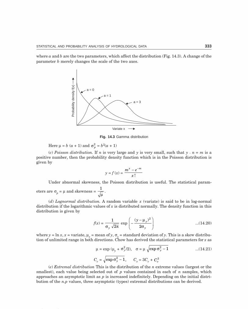
C-9\N-HYDRO\HYD14-1.PM5 333
STATISTICAL AND PROBABILITY ANALYSIS OF HYDROLOGICAL DATA 333
where a and b are the two parameters, which affect the distribution (Fig. 14.3). A change of theparameter b merely changes the scale of the two axes.
a = 0
a = 1
a = 3
Pro
babi
lity
dens
ityf(
x)
Variate x
Fig. 14.3 Gamma distribution
Here µ = b (a + 1) and σ p2 = b2(a + 1)
(c) Poisson distribution. If n is very large and y is very small, such that y . n = m is apositive number, then the probability density function which is in the Poisson distribution isgiven by
y = f (x) = m e
x
x m− −
!
Under abnormal skewness, the Poisson distribution is useful. The statistical param-
eters are σp = µ and skewness = 1
µ.
(d) Lognormal distribution. A random variable x (variate) is said to be in log-normaldistribution if the logarithmic values of x is distributed normally. The density function in thisdistribution is given by
f(x) = 1
2σ πy
exp −−F
HGIKJ
( )y y
y
µσ
2
2...(14.20)
where y = ln x, x = variate, µy = mean of y, σy = standard deviation of y. This is a skew distribu-tion of unlimited range in both directions. Chow has derived the statistical parameters for x as
µ = exp (µy + σ y2 /2), σ = µ exp σ y
2 1− ...(14.21)
Cv = exp σ y2 1− , Cs = 3Cv + Cv
3
(e) Extremal distribution This is the distribution of the n extreme values (largest or thesmallest), each value being selected out of p values contained in each of n samples, whichapproaches an asymptotic limit as p is increased indefinitely. Depending on the initial distri-bution of the n.p values, three asymptotic (types) extremal distributions can be derived.

C-9\N-HYDRO\HYD14-1.PM5 334
334 HYDROLOGY
(i) Type-I distribution In this distribution, the density function is given by
f(x) = 1c
exp −+F
HGIKJ − −
+FHG
IKJ
LNM
OQP
a xc
a xc
exp , –∞ < x < ∞ ...(14.22)
where x is the variate and a, c are the parameters. By the method of moments the parametershave been evaluated as
a = γc – µ, c = 6
π σ ...(14.23)
where γ = 0.57721 ... Euler’s constant. The distribution has a constant Cs = 1.139. The Gumbeldistribution used in flood frequency analysis is an example of this type.
(ii) Type-II distribution In this type, the cumulative probability is givenF(x) = exp [– (θ/x)k], –∞ < x < ∞ ...(14.24)
where θ and k are the parameters.(iii) Type-III distribution. In this type, the cumulative probability is given by
F(x) = exp −− ∈− ∈
FHG
IKJ
L
NMM
O
QPP
xk
θ , –∞ < x ≤ ε ...(14.25)
where θ and k are the parameters. Weibull distribution used in draught-frequency analy-sis is an example of this type.
(f ) Pearson’s Type-III distribution This is a skew distribution with limited range in theleft direction, usually bell shaped. The Pearson curve (Fig. 14.4), is truncated on one side of theaxis of the variate, i.e., below a certain value of the variate the probability is zero, but it isinfinite converging asymptotically to the axis of the variate. This means even values infinitelylarge (or small) have a certain probability of occurrence.
c.g.
Freq
uenc
y,(f
)
median
mode arith-mean Variate (x)0
Fig. 14.4 Pearson’s Type-III distribution
C-9\N-HYDRO\HYD14-1.PM5 335
STATISTICAL AND PROBABILITY ANALYSIS OF HYDROLOGICAL DATA 335
(g) Logarithmic Pearson Type-III distribution. This distribution has the advantage ofproviding a skew adjustment. If the skew is zero, the Log-Pearson distribution is identical tothe log-normal distribution.
The probability density function for type III (with origin at the mode) is
f(x) = f0 1 −FHG
IKJ
xa
c
exp (– cx/2) ...(14.26)
where c = 4β
– 1, a = c2
3
2
µµ
, β = µµ
32
22 ...(14.26 a)
f0 = na
ce c
c
c
+
+
1
1Γ( )...(14.26 b)
µ2 = the variance,µ3 = third moment about the mean = σ6g e = the base of the napierian logarithmsΓ = the gamma functionn = the number of years of recordg = the skew coefficientσ = the standard deviation
The US Water Resources Council (1967) adopted the Log-Pearson Type-III distribution(to achieve standardisation of procedures) for use by federal agencies. The procedure is toconvert the data series to logarithms and compute.
Mean: log x = Σ log x
n...(14.27)
Standard deviation: σlog x = Σ (log log )x x
n−−
2
1...(14.27 a)
Skew coefficient: g = n x xn n x
Σ (log log )( )( )( )log
−− −
3
31 2 σ ...(14.27 b)
The values of x for various recurrence intervals are computed from
log x = log x + K σlog x ...(14.28)
and the frequency factor K is obtained from Table 14.2 for the computed value of ‘g’ and thedesired recurrence interval (see Example 15.1).

C-9\N-HYDRO\HYD14-1.PM5 336
336 HYDROLOGY
Table 14.2. K-Values for the Log-Pearson Type-III Distribution
Skew Recurrence interval (T-yr)
coefficient 2 5 10 25 50 100 200
(g) Per cent chance (annual probability of occurrence P(%))
50 20 10 4 2 1 0.5
3.5 –0.396 0.420 1.180 2.278 3.152 4.051 4.970
2.5 –0.360 0.518 1.250 2.162 3.048 3.845 4.652
2.0 –0.307 0.609 1.302 2.219 2.912 3.605 4.298
1.8 –0.282 0.643 1.318 2.193 2.848 3.499 4.147
1.6 –0.254 0.675 1.329 2.163 2.780 3.388 3.990
1.4 –0.225 0.705 1.337 2.128 2.706 3.271 3.828
1.2 –0.195 0.732 1.340 2.087 2.626 3.149 3.661
1.0 –0.164 0.758 1.340 2.043 2.542 3.022 3.489
0.9 –0.148 0.769 1.339 2.018 2.498 2.957 3.401
0.8 –0.132 0.780 1.336 1.993 2.453 2.891 3.312
0.7 –0.116 0.790 1.333 1.967 2.407 2.824 3.223
0.6 –0.099 0.800 1.328 1.939 2.359 2.755 3.132
0.5 –0.083 0.808 1.323 1.910 2.311 2.686 3.041
0.4 –0.066 0.816 1.317 1.880 2.261 2.615 2.949
0.3 –0.050 0.823 1.309 1.849 2.211 2.544 2.856
0.2 –0.033 0.830 1.301 1.818 2.159 2.472 2.763
0.1 –0.017 0.836 1.292 1.785 2.107 2.400 2.670
0 0.000 0.841 1.282 1.751 2.054 2.326 2.576
–0.1 0.017 0.846 1.270 1.716 2.000 2.252 2.482
–0.2 0.033 0.850 1.258 1.680 1.945 2.178 2.388
–0.3 0.050 0.853 1.245 1.643 1.890 2.104 2.294
–0.4 0.066 0.855 1.231 1.606 1.834 2.029 2.201
–0.5 0.083 0.860 1.216 1.567 1.777 1.955 2.108
–0.6 0.099 0.857 1.200 1.528 1.720 1.880 2.016
–0.7 0.115 0.857 1.183 1.488 1.663 1.806 1.926
–0.8 0.132 0.856 1.166 1.448 1.606 1.733 1.837
–0.9 0.148 0.854 1.147 1.407 1.549 1.660 1.749
–1.0 0.164 0.852 1.128 1.366 1.492 1.588 1.664
–1.2 0.195 0.843 1.086 1.282 1.379 1.449 1.501
–1.4 0.225 0.832 1.041 1.198 1.270 1.318 1.351
–1.6 0.254 0.817 0.994 1.116 1.166 1.197 1.216
–1.8 0.282 0.799 0.945 1.035 1.069 1.087 1.097
–2.0 0.307 0.777 0.895 0.959 0.980 0.990 0.995
–2.5 0.360 0.710 0.771 0.793 0.798 0.799 0.800
–3.0 0.396 0.636 0.660 0.666 0.666 0.667 0.667

Chapter 15
337
FLOOD FREQUENCY—PROBABILITY
AND STOCHASTIC METHODS
15.1 FLOOD FREQUENCY METHODS
For the annual flood data of Lower Tapti River at Ukai (30 years: 1939–1968) in Example 8.5the flood frequencies of 2–, 10–, 50–, 100–, 200–, and 1000-year floods have been worked outbelow by the probability methods developed by Fuller, Gumbel, Powell, Ven Te Chow, andstochastic methods, and the flood frequency curves are drawn on a semi-log paper as shown inFig. 15.1. It can be seen that the Gumbel’s method gives the prediction of floods of a particularfrequency exceeding the observed floods by a safe margin and can be adopted in the design ofthe structure.
1. Fuller’s formula. QT = Q (1 + 0.8 log T) ...(15.1)
From Table 8.5, Q = 14.21 thousand cumec (tcm)
T log T 0.8 log T QT = Q (1 + 0.8 log T)
(tcm)
1000 3.0 2.4 48.3200 2.3010 1.8408 40.4100 2.0 1.6 37.0
50 1.6990 1.3592 33.510 1.0 0.8 25.6
2 0.3010 0.2408 17.35
2. Gumbel’s method. According to the extreme value distribution, the probability of occur-rence of a flood peak ≥ Q, is given by
P = 1 – e e y− −...(15.2)
the reduced variate y is given by
y = – 0.834 – 2.303 log log T
T − 1or, y = – 0.834 – 2.303 XT ...(15.3)
where XT = log log T
T − 1...(15.3 a)

C-9\N-HYDRO\HYD15-1.PM5 338
338 HYDROLOGY
The reduced variate y is linear with the variate Q (annual flood peak) itself and is givenby
y = σn Q Q−FHG
IKJσ
+ yn ...(15.4)
where σn (reduced standard deviation) and yn [reduced mean (to mode)] are functions of thesample size n and are given in Table 15.1.
∴ QT = Q + y yn
n
−FHG
IKJσ
σ ...(15.5)
or QT = Q + Kσ ...(15.6)
where the frequency factor K = y yn
n
−σ
and QT = annual flood peak, which has a recurrence
interval T.Since the coefficient of variation Cv = σ/Q
QT = Q (1 + KCv) ...(15.7)
The frequency factor K for the sample size n and the desired recurrence interval T canbe directly read from Table 15.2.
There are two approaches to the solution by the Gumbel’s method. The first approach is,for a given annual flood peak (QT), to find its recurrence interval T and probability of occur-rence P, for which the following sequence of tabulation should follow:
Table 15.1 Reduced mean ( yn ) and reduced standard deviation (σn)
as functions of sample size n
Size of sample n yn σn
10 0.4952 0.2457
15 0.5128 1.0206
20 0.5236 0.0628
25 0.5309 1.6915
30 0.5362 1.1124
35 0.5403 1.1283
40 0.5436 1.1413
45 0.5436 1.1518
50 0.5465 1.1607
55 0.5504 1.1681
60 0.5521 1.1747
65 0.5536 1.1803
70 0.5548 1.1854
75 0.5549 1.1898
(Contd.)...

C-9\N-HYDRO\HYD15-1.PM5 339
FLOOD FREQUENCY—PROBABILITY AND STOCHASTIC METHODS 339
80 0.5569 1.1938
85 0.5578 1.1973
90 0.5539 1.2007
95 0.5553 1.2038
100 0.5600 1.2065
200 0.5672 1.2359
500 0.5724 1.2588
1000 0.5745 1.2685
QT y XT T P = 1T
× 100
from Eq. (15.4) from Eq. (15.3) from Eq. (15.3 a) (%)
The second approach is, for a given recurrence interval T, to find the annual flood peakQT (which will be equalled or exceeded), for which the following sequence of tabulation shouldfollow; the computations are made for Lower Tapti river at Ukai.
XT = y = – 0.834 K* = y yn
n
−σ
QT† = Q + Kσ P = 1T
× 100
T (yr) log logT
T 1−FHG
IKJ – 2.3 XT (tcm) %
1000 –3.361 6.907 5.67 69.21 0.1
200 –2.662 5.295 4.23 55.51 0.5
100 –2.360 4.600 3.61 49.21 1.0
50 –2.056 3.901 3.02 43.51 2.0
10 –1.339 2.250 1.52 28.96 10
2 –0.521 0.366 –0.14 12.85 50
*(i) for the sample size n = 30, yn = 0.5362, σn = 1.1124.
(ii) for the desired T and the number of years of record n, the value of K can be directlyread from Table 15.2.
†Q = 14.21 tcm, σ = 9.7 tcm
Gumbel’s method can be viewed as a modification of the earlier probability methodsgiven by Eqs. (8.11, a and b) as
T = n
m c+ − 1...(15.8)
where c = Gumbel’s correction, and depends upon the ratio m/n, as given below:m/n: 1 0.9 0.8 0.7 0.6 0.5 0.4 0.3 0.2 0.1 0.08 0.04
c: 1 0.95 0.88 0.845 0.78 0.73 0.66 0.59 0.52 0.4 0.38 0.28

C-9\N-HYDRO\HYD15-1.PM5 340
340 HYDROLOGYY
ears
of
Rec
urr
ence
in
terv
al (
T–y
r)
reco
rd (
n)
25
1015
2025
3050
6075
100
200
400
1000
150.
967
1.70
32.
117
2.41
02.
632
2.82
33.
321
3.50
13.
721
4.00
56.
265
20–0
.147
0.91
91.
625
2.02
32.
302
2.51
72.
690
3.17
93.
352
3.56
33.
836
4.49
5.15
6.00
6
250.
888
1.57
51.
963
2.23
52.
444
2.61
43.
088
3.25
73.
463
3.72
95.
848
30–1
.152
0.86
61.
541
1.92
22.
188
2.39
32.
560
3.02
63.
191
3.39
33.
653
4.28
4.91
5.72
7
350.
851
1.51
61.
891
2.15
22.
354
2.52
02.
979
3.14
23.
341
3.59
8
40–0
.155
0.83
81.
495
1.86
62.
126
2.32
62.
489
2.94
33.
104
3.30
13.
554
4.16
4.78
5.57
6
450.
829
1.47
81.
847
2.10
42.
303
2.46
42.
913
3.07
83.
268
3.52
0
50–0
.156
0.82
01.
466
1.83
12.
086
2.28
32.
443
2.88
93.
048
3.24
13.
491
4.08
4.56
5.47
8
550.
813
1.45
51.
818
2.07
12.
267
2.42
62.
869
2.02
73.
219
3.46
7
600.
807
1.44
61.
806
2.05
92.
253
2.41
12.
852
3.00
83.
200
3.44
6
650.
801
1.43
71.
796
2.04
82.
241
2.39
82.
837
2.99
23.
183
3.42
9
700.
797
1.43
01.
788
2.03
82.
230
2.38
72.
824
2.97
93.
169
3.41
35.
359
750.
792
1.42
31.
780
2.02
92.
220
2.37
72.
812
2.96
73.
155
3.40
0
800.
788
1.41
71.
773
2.02
02.
212
2.36
82.
802
2.95
63.
145
3.38
7
850.
785
1.41
31.
767
2.01
32.
205
2.36
12.
793
2.94
63.
135
3.37
6
900.
782
1.40
91.
762
2.00
72.
198
2.35
32.
785
2.93
83.
125
2.36
7
950.
780
1.40
51.
757
2.00
22.
193
2.34
72.
777
2.93
03.
116
3.35
7
100
–0.1
600.
779
1.40
11.
752
1.99
82.
187
2.34
12.
770
2.92
23.
109
3.34
93.
934.
515.
261
Tab
le 1
5.2
Fre
quen
cy f
acto
r (K
) fo
r G
um
bel’s
met
hod
. (e
xtre
mal
val
ue:
Typ
e-I
dist
ribu
tion
)
C-9\N-HYDRO\HYD15-1.PM5 341
FLOOD FREQUENCY—PROBABILITY AND STOCHASTIC METHODS 341
3. Powell method. A modification in the value of K in Eq. (15.6) was made by R.W. Powell(1943)
K = – 6
π γ +
−LNM
OQP
ln lnT
T 1 ...(15.9)
where γ = Euler’s constant = 0.5772 .... ln = loge
Simplifying, K = –1.1 – 1.795 XT ...(15.10)
Then QT = Q + Kσ ...(15.11)
The computations are made for lower Tapi river at Ukai as per Powell method, below:
XT = K = – 1.1
T log logT
T 1−FHG
IKJ – 1.795 XT Kσ∗ QT = Q + Kσ P =
1T
× 100
(yr) (tcm) (%)
1000 –3.361 4.93 47.8 62.01 0.1
200 –2.662 3.68 35.8 50.01 0.5
100 –2.360 3.13 30.4 44.61 1.0
50 –2.056 2.58 25.0 39.21 2.0
10 –1.339 1.30 12.6 26.81 10
2 –0.521 –0.164 –1.6 12.62 50
*Q = 14.21 tcm, σ = 9.7 tcm
4. Ven Te Chow method. Another modification of the Gumbel’s method was made by V.T.Chow by using the frequency factor. The equation is
QT = a + bXT ...(15.12)
where XT = log log1
TT −
FHG
IKJ ...(15.12 a)
a, b = parameters estimated by the method of moments from the observed data. The followingequations are derived from the method of least squares.
Σ Q = an + b Σ XT
Σ (QXT) = a Σ XT + bΣ (XT2) ...(15.13)
from which a and b can be solved.In this method, a plotting position has been assigned for each value of Q when arranged
in the descending order or magnitude of flood peaks. For example, if an annual flood peak QThas a rank m, its plotting position
T = n
m+ 1
...(15.14)
From Eq. (15.12 a),
XT = log log1
TT −
FHG
IKJ

C-9\N-HYDRO\HYD15-1.PM5 342
342 HYDROLOGY
putting the value of T from Eq. (15.14)
XT = log logn
n m+
+ −FHG
IKJ
11
...(15.15)
The computation is made in Table 15.3 for Lower Tapi river at Ukai.
Table 15.3 Computation for determining a, b: Ven Te Chow method
Order no. Flood peak XT = log logn 1
n 1 m+
+ −FHG
IKJ QXT XT
2
(m) Q (tcm)
1 42.45 –1.848 –78.4 3.41
2 37.30 –1.538 –57.4 2.37
3 29.30 –1.468 –43.0 2.15
4 24.20 –1.223 –29.6 1.50
5 22.62 –1.119 –25.3 1.25
6 21.24 –1.032 –21.9 1.06
7 20.86 –0.965 –20.1 0.93
8 19.65 –0.886 –17.4 0.79
9 18.70 –0.830 –15.5 0.69
10 18.30 –0.794 –14.5 0.63
11 14.57 –0.718 –10.5 0.52
12 14.00 –0.672 –9.4 0.45
13 12.88 –0.627 –8.1 0.39
14 12.45 –0.585 –7.3 0.34
15 11.43 –0.542 –6.2 0.29
16 10.34 –0.502 –4.9 0.25
17 9.72 –0.462 –4.5 0.21
18 9.68 –0.434 –4.2 0.19
19 8.50 –0.386 –3.3 0.15
20 8.44 –0.347 –2.9 0.12
21 7.65 –0.308 –2.4 0.09
22 7.27 –0.270 –2.0 0.07
23 7.22 –0.230 –1.7 0.05
24 6.48 –0.190 –1.2 0.04
25 6.23 –0.146 –0.9 0.02
26 6.09 –0.102 –0.6 0.01
27 5.81 –0.051 –0.3 0.03
28 4.82 0.006 0.03 0.000036
29 4.39 0.077 0.34 0.0059
30 3.68 0.174 0.64 0.0303
Σn = 30 426.27 – 16.00 – 392.30 18.04

C-9\N-HYDRO\HYD15-1.PM5 343
FLOOD FREQUENCY—PROBABILITY AND STOCHASTIC METHODS 343
00
00
0000
00
00
Q= 3.68 + 24.26 Log T : S
tochasti
c
TQ= 3.68 + 24.26 Log T : S
tochasti
c
T
Q= 14.21 + 9.7(
) : Gumbel
TQ= 14.21 + 9.7(
) : Gumbel
T
y – 0.54
1.1124y – 0.54
1.1124
Q= 4.94 – :17.4 log (log
): V.T. Chow
TQ= 4.94 – :17.4 log (log
): V.T. Chow
T
Q= 14.21 + 9.7 (– 1.1 – 1.795 log (log
))
TQ= 14.21 + 9.7 (– 1.1 – 1.795 log (log
))
T
TT – 1TT – 1
TT – 1TT – 1
Q =14.21(1 + 0.8 log T) : Fuller
TQ =14.21(1 + 0.8 log T) : Fuller
T
93 - yr observed flood
93 - yr observed floodFoster : Q = 14.21 + 9.7 K
IT
Foster : Q = 14.21 + 9.7 K
IT
unsafeunsafe
Foster-typeQ = 14.21 + 9.7 K [Ex. 8.5 (b)]
I
T
Foster-typeQ = 14.21 + 9.7 K [Ex. 8.5 (b)]
I
T
powellpowell
1968 flood42.5 tcm
1959 flood37.3 bcmII
IHigh flood peaksduring 1876-1968:
93-years
Flood frequencylines
Annual flood data oflower Tapi river
at Ukai: 1939-1968(Western India)
Semi-log paper
P = 100 % of time´90
80
70
60
50
40
30
20
10
100 50 25 10 5 2 1 0.5 0.2 0.1Probability or % chance of a flood > Q in any one yearT
Flo
odpe
akQ
(100
0cu
mec
)T
2 3 4 5 6 8 20 30 50 70 90 200 500 2 3100010010
Recurrence interval (T-yr)
1
Safe
Fig. 15.1 Flood frequency curves of lower Tapi at Ukai (1939-1968)
Substituting the values in Eq. (15.13)426.27 = 30a – 16b
– 392.30 = – 16a + 18.04bSolving the equations
a = 4.94, b = – 17.4Then QT = a + bXT ∴ QT = 4.94 – 17.4 XT ...(15.16)The computations are made for Lower Tapi river at Ukai as per Ven Te Cow method,
below.
T XT = QT =
(yr) log logT
T 1−FHG
IKJ 4.94 – 17.4 Xt P =
1T
× 100
(tcm) (%)
1000 –3.361 63.44 0.1200 –2.662 51.34 0.5100 –2.360 46.04 1
50 –2.056 40.64 210 –1.339 28.29 10
2 –0.521 14.02 50
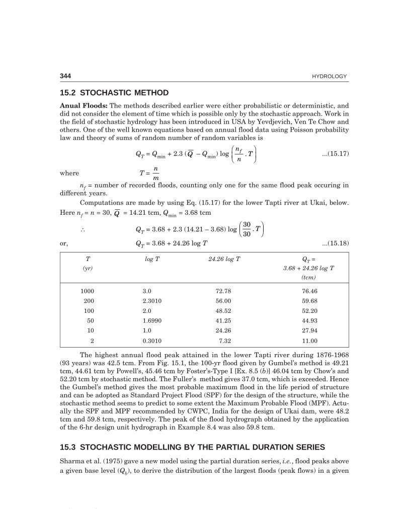
C-9\N-HYDRO\HYD15-1.PM5 344
344 HYDROLOGY
15.2 STOCHASTIC METHOD
Anual Floods: The methods described earlier were either probabilistic or deterministic, anddid not consider the element of time which is possible only by the stochastic approach. Work inthe field of stochastic hydrology has been introduced in USA by Yevdjevich, Ven Te Chow andothers. One of the well known equations based on annual flood data using Poisson probabilitylaw and theory of sums of random number of random variables is
QT = Qmin + 2.3 (Q – Qmin) log n
nTf .
FHG
IKJ ...(15.17)
where T = nm
nf = number of recorded floods, counting only one for the same flood peak occuring indifferent years.
Computations are made by using Eq. (15.17) for the lower Tapti river at Ukai, below.Here nf = n = 30, Q = 14.21 tcm, Qmin = 3.68 tcm
∴ QT = 3.68 + 2.3 (14.21 – 3.68) log 3030
. TFHG
IKJ
or, QT = 3.68 + 24.26 log T ...(15.18)
T log T 24.26 log T QT =
(yr) 3.68 + 24.26 log T
(tcm)
1000 3.0 72.78 76.46
200 2.3010 56.00 59.68
100 2.0 48.52 52.20
50 1.6990 41.25 44.93
10 1.0 24.26 27.94
2 0.3010 7.32 11.00
The highest annual flood peak attained in the lower Tapti river during 1876-1968(93 years) was 42.5 tcm. From Fig. 15.1, the 100-yr flood given by Gumbel’s method is 49.21tcm, 44.61 tcm by Powell’s, 45.46 tcm by Foster’s-Type I [Ex. 8.5 (b)] 46.04 tcm by Chow’s and52.20 tcm by stochastic method. The Fuller’s method gives 37.0 tcm, which is exceeded. Hencethe Gumbel’s method gives the most probable maximum flood in the life period of structureand can be adopted as Standard Project Flood (SPF) for the design of the structure, while thestochastic method seems to predict to some extent the Maximum Probable Flood (MPF). Actu-ally the SPF and MPF recommended by CWPC, India for the design of Ukai dam, were 48.2tcm and 59.8 tcm, respectively. The peak of the flood hydrograph obtained by the applicationof the 6-hr design unit hydrograph in Example 8.4 was also 59.8 tcm.
15.3 STOCHASTIC MODELLING BY THE PARTIAL DURATION SERIES
Sharma et al. (1975) gave a new model using the partial duration series, i.e., flood peaks abovea given base level (Qb), to derive the distribution of the largest floods (peak flows) in a given

C-9\N-HYDRO\HYD15-1.PM5 345
FLOOD FREQUENCY—PROBABILITY AND STOCHASTIC METHODS 345
time interval (0, t). The magnitude of these peaks are considered as a series of random vari-ables. The base flow Qb may be taken as the bankfull discharge of the river at the particularstation. If Qi is the flood peak, which has occurred in the time interval (0, t), then the floodexceedance xi in this interval is
xi = Qi – Qb ...(15.19)
The number n(t) of flood exceedances in an interval of time (0, t) as well as the magnitudesof the exceedances x(t), are time, dependent-random variables. The time Ti of ocurrence ofthese exceedances are also random variables. The time Ti is assoiated with the random vari-ables xi for i = 1, 2, 3, ... n.
Todorovic and Emir Zelenhasic (1970) have developed the distribution function Ft(x) ofthe largest exceedance in a given interval of time (0, t) as
Ft(x) = exp (– λ t e–βx) ...(15.20)
and the probability of occurrence of exceedances xi during the interval (0, t) as
H(x) = 1 – exp (– βx) ...(15.21)
For a particular exceedance xT for an interval of T years
F(xT) = exp [– λT e xT− β ] ...(15.22)
where λ and β are constants for a particular series of data (λ = average number of exceedancesper year).
If xT ≥ 0 for T ≥ 0, then F(xT) will represent the probability of occurrence of an exceedancexT and
F(xT) = 1
λT...(15.23)
From eqs. (15.22) and (15.23), the new mathematical model is obtained as
xT = 1β
[ln (λ.T) – ln {ln (λ.T)}] ...(15.24)
Then, the design flood QT may be obtained as
QT = Qb + xT ...(15.25)
Example 15.1 Flood data in the form of Partial-Duration Series and Annual-Flood Peaks forthe Ganga river at Hardwar for a period of 87 years (1885-1971) are given in Tables 15.4 and15.5, respectively. The base flow for the partial duration series may be taken as 4333 cumec(which was accepted as the bankfull discharge in the design of weir at Bhimgoda).
Derive the flood-frequency curves based on the two series by using the stochastic models.Make a comparative study with the other methods based on annual floods discussed earlier.
[Note Partial duration series data for the Lower Tapti river at Ukai could not be ob-tained and hence flood data for the Ganga river is given here].

C-9\N-HYDRO\HYD15-1.PM5 346
346 HYDROLOGY
St.
no.
Yea
rC
um
ecJ
un
eD
t.J
uly
Dt.
Au
g.D
t.S
ept.
Dt.
Oct
.D
t.
12
34
56
78
910
1112
13
1.18
85Q
5814
1672
419
x14
8129
08
2.18
86Q
4665
1591
635
6018
2
x33
248
3116
85
Q48
4822
x51
5
Q43
6927
x36
3.18
87Q
5882
2
x15
49
Q74
0722
x30
74
4.18
88Q
5417
2248
482
5417
3
x10
8451
510
84
Q50
3427
6870
20
x70
125
37
Q49
0931
x57
6
5.18
89Q
5680
2579
367
7546
349
719
x13
4736
0332
1363
8
Q48
4817
9855
15
x51
555
22
Q88
2729
7857
29
x44
9435
24
Tab
le 1
5.4.
Par
tial
du
rati
on s
erie
s of
flo
ods
for
the
rive
r G
anga
at
Har
dwar
du
rin
g 18
85-1
971
(87
year
s).
Bas
e fl
ow,
Qb
= 43
33 c
umec
, Q
= F
lood
pea
k, x
= F
lood
pea
k ex
ceed
ance
. (E
xam
ple
15.1
).
(Con
td.)
...
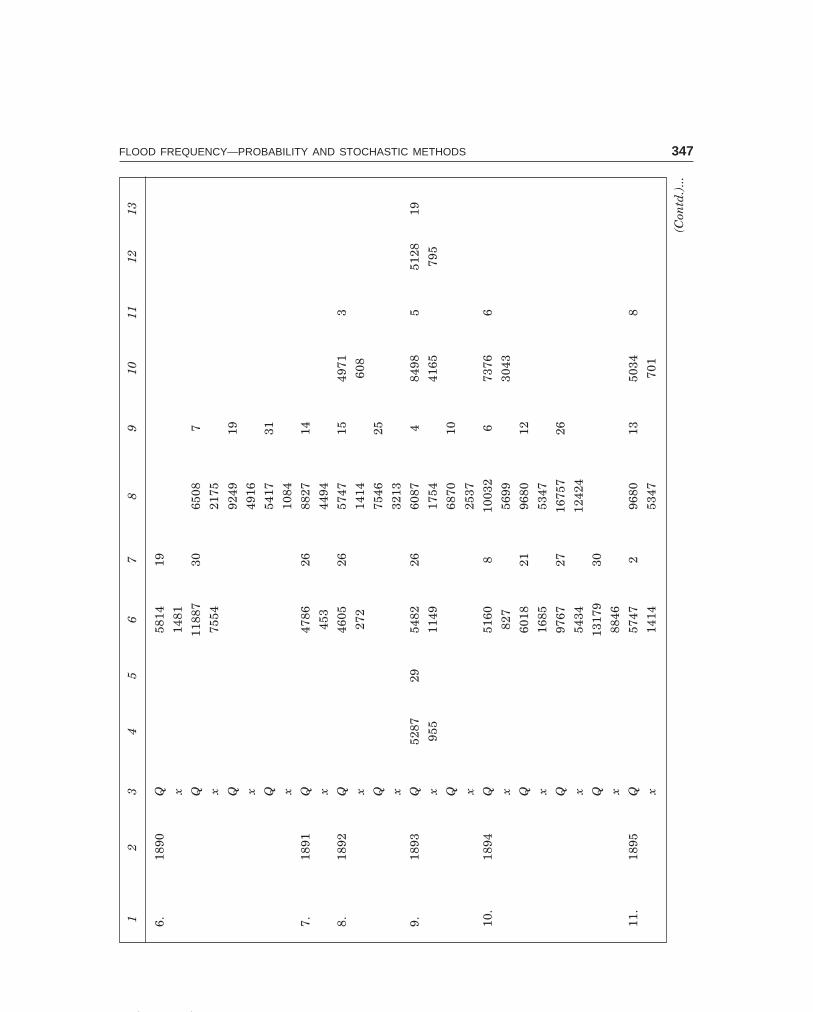
C-9\N-HYDRO\HYD15-1.PM5 347
FLOOD FREQUENCY—PROBABILITY AND STOCHASTIC METHODS 3471
23
45
67
89
1011
1213
6.18
90Q
5814
19
x14
81
Q11
887
3065
087
x75
5421
75
Q92
4919
x49
16
Q54
1731
x10
84
7.18
91Q
4786
2688
2714
x45
344
94
8.18
92Q
4605
2657
4715
4971
3
x27
214
1460
8
Q75
4625
x32
13
9.18
93Q
5287
2954
8226
6087
484
985
5128
19
x95
511
4917
5441
6579
5
Q68
7010
x25
37
10.
1894
Q51
608
1003
26
7376
6
x82
756
9930
43
Q60
1821
9680
12
x16
8553
47
Q97
6727
1675
726
x54
3412
424
Q13
179
30
x88
46
11.
1895
Q57
472
9680
1350
348
x14
1453
4770
1
(Con
td.)
...

C-9\N-HYDRO\HYD15-1.PM5 348
348 HYDROLOGY
12
34
56
78
910
1112
13
1218
96Q
1433
610
x10
003
13.
1897
Q76
2322
7407
544
273
x32
9030
7494
Q81
7423
x38
41
14.
1898
Q58
1410
8953
1263
667
x14
8146
2020
33
Q58
8224
7241
18
x15
4929
08
15.
1899
Q75
4623
x32
13
16.
1900
Q44
8617
6651
1159
506
x15
323
1816
17
Q50
9726
4786
12
x76
445
3
17.
1901
Q44
2719
7700
8
x94
3367
Q11
409
24
x70
76
18.
1902
Q91
633
4848
14
x48
3051
5
19.
1903
Q74
0714
x30
74
Q62
9627
x19
63
20.
1904
Q85
7929
7092
3
x42
4627
59
(Con
td.)
...

C-9\N-HYDRO\HYD15-1.PM5 349
FLOOD FREQUENCY—PROBABILITY AND STOCHASTIC METHODS 3491
23
45
67
89
1011
1213
Q70
9112
x27
58
Q70
1721
x26
84
21.
1905
Q93
6213
x50
29
22.
1906
Q70
9228
6870
362
2616
x27
5925
3718
93
Q59
5019
x16
17
23.
1907
Q75
4630
7241
3
x32
1329
08
24.
1908
Q66
5113
1150
42
x23
1871
71
Q59
4921
x16
16
Q60
1829
x16
85
25.
1909
Q68
7016
7407
12
x25
3730
74
Q83
3521
6724
20
x40
0223
91
Q59
4927
x16
16
26.
1910
Q46
0515
1012
128
7469
361
5611
1507
73
x27
257
8831
3618
2310
744
Q11
887
13
x75
54
(Con
td.)
...

C-9\N-HYDRO\HYD15-1.PM5 350
350 HYDROLOGY
12
34
56
78
910
1112
13
Q70
9118
x27
59
27.
1911
Q69
4318
4369
13
x26
1036
28.
1912
Q77
0016
8335
2
x33
6740
02
29.
1914
Q54
172
9249
19
x10
8449
16
Q60
1828
x16
85
3019
15Q
6579
2
x22
46
Q74
0713
x30
74
Q47
2529
x39
2
31.
1916
Q47
2526
x39
2
32.
1917
Q84
1611
5352
554
829
x40
8310
1911
49
Q68
7025
4909
23
x25
3757
6
33.
1918
Q46
6522
x33
2
34.
1919
Q62
9613
5160
7
x19
6382
7
35.
1920
Q48
4823
8174
14
x51
538
41
(Con
td.)
...

C-9\N-HYDRO\HYD15-1.PM5 351
FLOOD FREQUENCY—PROBABILITY AND STOCHASTIC METHODS 3511
23
45
67
89
1011
1213
36.
1921
Q56
8026
7623
465
089
x13
4732
9021
75
9079
1859
5015
4746
1617
37.
1922
Q58
1420
7407
1750
343
x14
8130
7470
1
38.
1923
Q54
825
x11
49
39.
1924
Q51
6027
6087
348
485
x82
717
5451
5
Q50
9719
1913
629
x76
414
803
40.
1925
Q51
6021
9670
12
x82
753
47
41.
1927
Q72
365
x29
03
Q72
4120
x29
08
42.
1929
Q45
4515
x21
2
43.
1930
Q54
4327
5997
21
x11
1016
64
44.
1932
Q55
3214
x11
99
6155
24
1822
45.
1933
Q46
9225
5267
15
x35
993
4
(Con
td.)
...

C-9\N-HYDRO\HYD15-1.PM5 352
352 HYDROLOGY
12
34
56
78
910
1112
13
46.
1934
Q61
9321
x18
60
47.
1935
Q52
894
x95
6
48.
1942
Q48
8724
6650
9
x55
423
17
49.
1943
Q44
4222
x10
9
50.
1945
Q48
3619
5101
3
x50
376
8
51.
1946
Q46
2928
x29
6
52.
1947
Q43
4527
x12
53.
1948
Q48
9025
x55
7
54.
1950
Q45
6226
5899
18
x22
915
66
55.
1951
Q44
5822
4339
15
x12
56
56.
1953
Q54
7013
x11
37
57.
1954
Q59
7820
x16
45
58.
1955
Q46
445
x31
1
59.
1956
Q63
8111
x20
48
(Con
td.)
...

C-9\N-HYDRO\HYD15-1.PM5 353
FLOOD FREQUENCY—PROBABILITY AND STOCHASTIC METHODS 3531
23
45
67
89
1011
1213
60.
1957
Q45
4815
x21
3
61.
1959
Q44
933
x16
0
62.
1961
Q48
5517
x52
2
63.
1962
Q57
6028
x14
27
64.
1963
Q55
7421
9192
17
x12
4148
59
65.
1966
Q47
4126
x40
8
66.
1967
Q59
1927
x15
86
67.
1969
Q45
4620
x21
3
68.
1971
Q45
427
x20
9

C-9\N-HYDRO\HYD15-2.PM5 354
354 HYDROLOGY
Table 15.5 Annual Peak discharges for Ganga river at Hardwarfor the period 1885-1971 (87 yrs) (Example 15.1)
Sl. Year Ann. Peak Log10 Q Sl. Year Ann. Peak Log10 Qno. Q (cumec) no. Q (cumec)
(Contd.)...
1. 1885 7241 3.8598
2. 1886 9164 3.9621
3. 1887 7407 3.8696
4. 1888 6870 3.8370
5. 1889 9855 3.9936
6. 1890 11887 4.0752
7. 1891 8827 3.9458
8. 1892 7546 3.8777
9. 1893 8498 3.9293
10. 1894 16757 4.2242
11. 1895 9680 3.9859
12. 1896 14336 4.1565
13. 1897 8174 3.9124
14. 1898 8953 3.9518
15. 1899 7546 3.8777
16. 1900 6652 3.8229
17. 1901 11409 4.0573
18. 1902 9164 3.9621
19. 1903 7404 3.8694
20. 1904 8579 3.9335
21. 1905 9362 3.9714
22. 1906 7092 3.8507
23. 1907 7546 3.8777
24. 1908 11504 4.0607
25. 1909 8335 3.9209
26. 1910 15077 4.1783
27. 1911 6943 3.8416
28. 1912 8335 3.9209
29. 1913 3579 3.5538
30. 1914 9299 3.9684
31. 1915 7407 3.8696
32. 1916 4726 3.6744
33. 1917 8416 3.9251
34. 1918 4668 3.6698
35. 1919 6296 3.7991
36. 1920 8174 3.9124
37. 1921 9079 3.9580
38. 1922 7407 3.8696
39. 1923 5482 3.7390
40. 1924 19136 4.2818
41. 1925 9680 3.9859
42. 1926 3698 3.5680
43. 1927 7241 3.8598
44. 1928 3698 3.5680
45. 1929 4545 3.6576
46. 1930 5998 3.7780
47. 1931 3470 3.5403
48. 1932 6155 3.7893
49. 1933 5267 3.7216
50. 1934 6193 3.7919
51. 1935 5289 3.7223
52. 1936 3320 3.5211
53. 1937 3232 3.5095
54. 1938 3525 3.5471
55. 1939 2341 3.3694
56. 1940 2429 3.3854
57. 1941 3154 3.4989
58. 1942 6650 3.8228
59. 1943 4442 3.6476
60. 1944 4229 3.6262
61. 1945 5101 3.7077
62. 1946 4629 3.6654
63. 1947 4345 3.6380
64. 1948 4890 3.6893
65. 1949 3619 3.5586
66. 1950 5899 3.7708
67. 1951 4458 3.6492
68. 1952 3919 3.5932
69. 1953 5470 3.7380
70. 1954 5978 3.7766
71. 1955 4644 3.6669
72. 1956 6381 3.8049
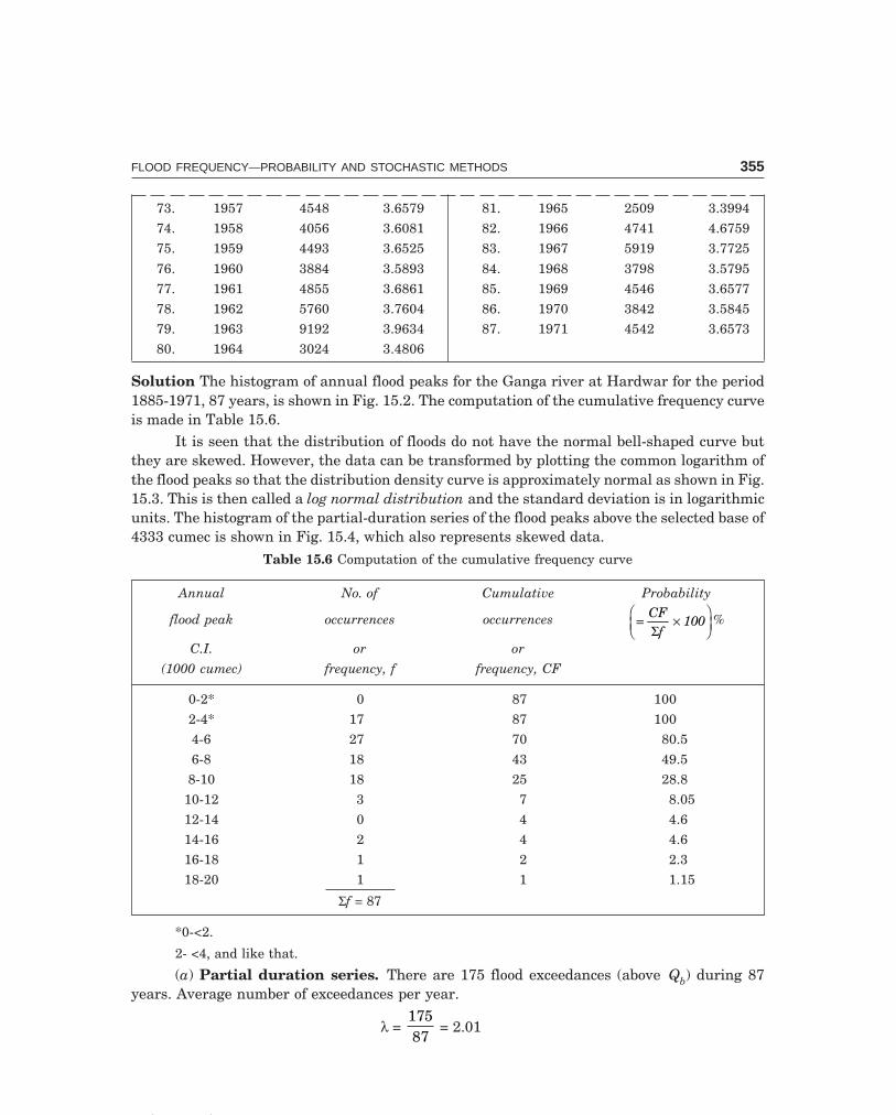
C-9\N-HYDRO\HYD15-2.PM5 355
FLOOD FREQUENCY—PROBABILITY AND STOCHASTIC METHODS 355
Solution The histogram of annual flood peaks for the Ganga river at Hardwar for the period1885-1971, 87 years, is shown in Fig. 15.2. The computation of the cumulative frequency curveis made in Table 15.6.
It is seen that the distribution of floods do not have the normal bell-shaped curve butthey are skewed. However, the data can be transformed by plotting the common logarithm ofthe flood peaks so that the distribution density curve is approximately normal as shown in Fig.15.3. This is then called a log normal distribution and the standard deviation is in logarithmicunits. The histogram of the partial-duration series of the flood peaks above the selected base of4333 cumec is shown in Fig. 15.4, which also represents skewed data.
Table 15.6 Computation of the cumulative frequency curve
Annual No. of Cumulative Probability
flood peak occurrences occurrences = ×FHG
IKJ
CFf
100Σ
%
C.I. or or
(1000 cumec) frequency, f frequency, CF
0-2* 0 87 100
2-4* 17 87 100
4-6 27 70 80.5
6-8 18 43 49.5
8-10 18 25 28.8
10-12 3 7 8.05
12-14 0 4 4.6
14-16 2 4 4.6
16-18 1 2 2.3
18-20 1 1 1.15
Σf = 87
*0-<2.
2- <4, and like that.
(a) Partial duration series. There are 175 flood exceedances (above Qb) during 87years. Average number of exceedances per year.
λ = 17587
= 2.01
73. 1957 4548 3.6579
74. 1958 4056 3.6081
75. 1959 4493 3.6525
76. 1960 3884 3.5893
77. 1961 4855 3.6861
78. 1962 5760 3.7604
79. 1963 9192 3.9634
80. 1964 3024 3.4806
81. 1965 2509 3.3994
82. 1966 4741 4.6759
83. 1967 5919 3.7725
84. 1968 3798 3.5795
85. 1969 4546 3.6577
86. 1970 3842 3.5845
87. 1971 4542 3.6573

C-9\N-HYDRO\HYD15-2.PM5 356
356 HYDROLOGY
Parameter β is estimated in the following Table.
Sl. Flood peak exceedance Observed Cumulative H(x) 1 – H(x) β
no. xi (cumec) frequency frequency = CF175
= − −1n {1 H(x)}
xCI Variable CF ...× 10–4
1. below-2500 2500 107 107 0.6114 0.3886 3.362
2. 2500-5000 5000 51 158 0.9029 0.0971 4.649
3. 5000-7500 7500 10 168 0.9600 0.0400 4.282
4. 7500-10000 10000 3 171 0.9771 0.0229 3.762
5. 10000-12500 12500 3 174 0.9443 0.0057 4.119
6. 12500-15000 15000 1 175 1.0000 0.0000 —
Mean = 6635 cumecMedian = 7000 cumecMode = 5000 cumecCumulativefrequency (%) curve
100
80
60 50 %
40
20
00 2 4 6 8 10 12 14 16 18 20
Q (1000 cumec)
Pro
babi
lity
(%)
Med
ian
Histogram
Normalcurve(Mean = median = mode)
Frequencycurve - skewed
Modal class
f = 27 max.
Freq
uenc
yor
no.o
f occ
urre
nces
30
25
20
15
10
5
0
0-2
2-4
4-6
8-10
10-1
2
12-1
4
14-1
6
16-1
8
18-2
0
C of Q (1000 cumec)I
LmdC.I.7 x
Mod
eM
ode
Cen
ter
ofgr
avity
Cen
ter
ofgr
avity
Mea
n.M
ean.
Med
ian
Med
ian
d1
d2
c.g.c.g.
Fig. 15.2 Histogram of annual floods of river Ganga (1885-1971)
� ������� �������

C-9\N-HYDRO\HYD15-2.PM5 357
FLOOD FREQUENCY—PROBABILITY AND STOCHASTIC METHODS 357
Log normal (skew = 0)curveLog - pearson (skew = 0.81)III
Histogram
No.
ofoc
curr
ence
s
50
40
30
20
10
0
3.0-
3.2
3.2-
3.4
3.4-
3.6
3.6-
3.8
3.8-
4.0
4.0-
4.2
4.2-
4.4
C. of Log Q (cumec)
Fig. 15.3 Histogram of logarithm of annual floods of river Ganga (1885-1971)
100
90
80
70
60
50
40
30
20
10
0
No.
ofoc
curr
ence
s
Skewed distributionof partial duration floods
0-2
2-4
4-6
6-8
8-10
10-1
2
12-1
4
14-1
6
16-1
8
18-2
0
C of Q (1000 cumec) (>Q = 4333 cumec)I b
Fig. 15.4 Histogram of partial duration floods in river Ganga (1885–1971)
The average value of β = �β = 4.05 × 10⁻⁴
Estimation of design flood can now be done from Eqs. (15.24) and (15.25)QT = Qb + xT
∴ QT = 4333 + 104 05
4
. [ln (2.01 T) – ln {ln (2.01 T)}] ...(15.26)
T-yr: 1000 500 200 100 50
QT (cumec): 18103 16605 14728 13296 11938
QT by T =n 1
m+
: 23600 21600 18900 17000 15100
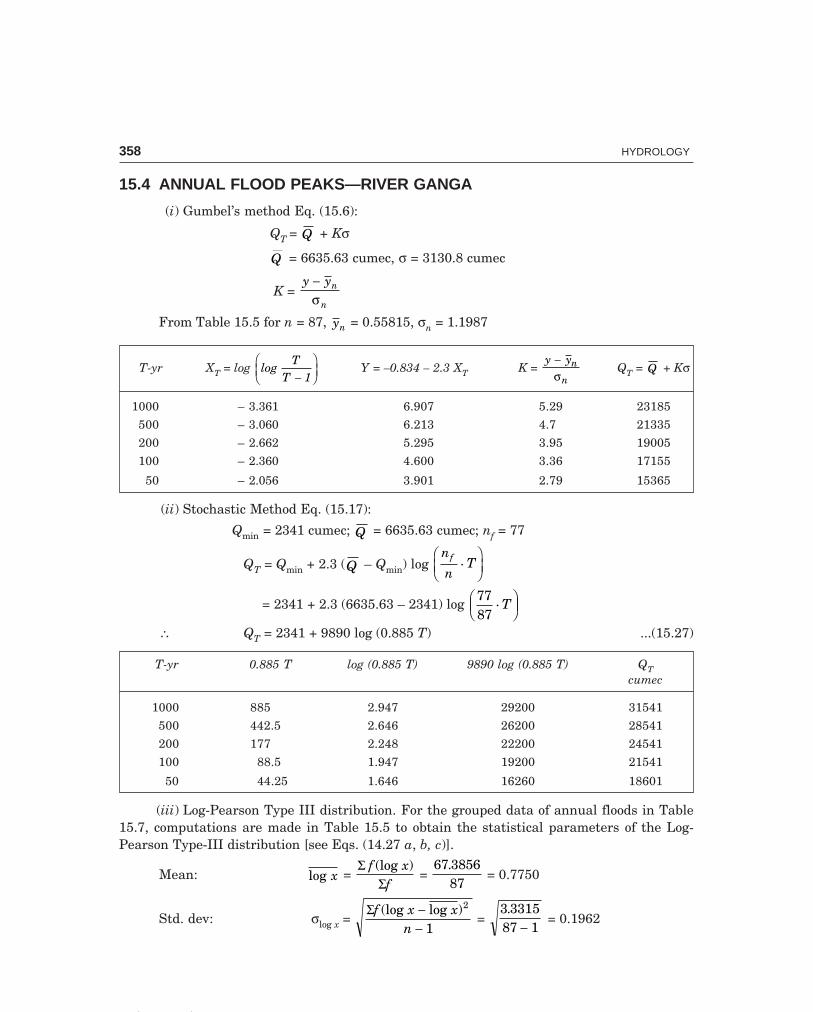
C-9\N-HYDRO\HYD15-2.PM5 358
358 HYDROLOGY
15.4 ANNUAL FLOOD PEAKS—RIVER GANGA
(i) Gumbel’s method Eq. (15.6):
QT = Q + Kσ
Q = 6635.63 cumec, σ = 3130.8 cumec
K = y yn
n
−σ
From Table 15.5 for n = 87, yn = 0.55815, σn = 1.1987
T-yr XT = log logT
T 1−FHG
IKJ Y = –0.834 – 2.3 XT K =
y yn
n
−σ
QT = Q + Kσ
1000 – 3.361 6.907 5.29 23185
500 – 3.060 6.213 4.7 21335
200 – 2.662 5.295 3.95 19005
100 – 2.360 4.600 3.36 17155
50 – 2.056 3.901 2.79 15365
(ii) Stochastic Method Eq. (15.17):
Qmin = 2341 cumec; Q = 6635.63 cumec; nf = 77
QT = Qmin + 2.3 (Q – Qmin) log n
nTf .F
HGIKJ
= 2341 + 2.3 (6635.63 – 2341) log 7787
. TFHG
IKJ
∴ QT = 2341 + 9890 log (0.885 T) ...(15.27)
T-yr 0.885 T log (0.885 T) 9890 log (0.885 T) QTcumec
1000 885 2.947 29200 31541
500 442.5 2.646 26200 28541
200 177 2.248 22200 24541
100 88.5 1.947 19200 21541
50 44.25 1.646 16260 18601
(iii) Log-Pearson Type III distribution. For the grouped data of annual floods in Table15.7, computations are made in Table 15.5 to obtain the statistical parameters of the Log-Pearson Type-III distribution [see Eqs. (14.27 a, b, c)].
Mean: log x = Σ
Σf x
f(log )
= 67 3856
87.
= 0.7750
Std. dev: σlog x = Σf x x
n(log log )−
−
2
1 =
3 331587 1.
− = 0.1962

C-9\N-HYDRO\HYD15-2.PM5 359
FLOOD FREQUENCY—PROBABILITY AND STOCHASTIC METHODS 359C
IM
id-p
t. o
f C
IF
requ
ency
(100
0x
flo
g x
f lo
g x
log
x(l
og x
(log
xf(
log
xf(
log
x
cum
ec)
(100
0 cu
mec
)–
log
x–
log
x)2
– lo
gx
)3–
log
x)2
– lo
gx
)3
0-2
10
00
00
00
0
2-4
317
0.47
718.
1000
–0.2
979
–0.0
890
–0.0
265
1.51
20–0
.450
0
4-6
527
0.69
9018
.900
0–0
.076
00.
0058
–0.0
0044
0.15
60–0
.011
9
6-8
718
0.84
5115
.200
00.
0701
0.00
490.
0003
0.08
850.
0062
8-10
918
0.95
4217
.200
00.
1792
0.03
400.
0057
0.57
900.
1025
10-1
211
31.
0414
3.12
420.
2664
0.07
100.
0190
0.21
300.
0570
12-1
413
01.
1139
0.00
000.
3389
0.11
500.
0390
0.00
000.
0000
14-1
615
21.
1761
2.35
220.
4011
0.16
100.
0644
0.32
200.
1288
16-1
817
11.
2304
1.23
040.
4554
0.20
700.
0940
0.20
700.
0940
18-2
019
11.
2788
1.27
880.
5038
0.25
400.
1280
0.25
400.
1280
Σn
= Σf
= 8
7Σf
. lo
g (x
) =
67.3
856
3.33
150.
5165
For
gro
upe
d da
ta:
log
x =
ΣΣ
fx
f. l
og(
) = 67
3856
87. =
0.7
750
Tab
le 1
5.7.
Log
-Pea
rson
Typ
e-II
I di
stri
buti
on f
or t
he
ann
ual
flo
ods
of r
iver
Gan
ga (
1885
-197
1) (
Exa
mpl
e 15
.1)

C-9\N-HYDRO\HYD15-2.PM5 360
360 HYDROLOGY
Skew: g = n f x xn n x
Σ (log log )( )( )( )
( . )( )( )( . )log
−− −
=− −
3
3 31 287 0 5165
87 1 87 2 0 1962σ = 0.81
Putting variate x = flood peak Q(1000 cumec), the distribution Eq. (14.28) becomes
log QT = log Q + Kσlog Q ...(15.28)and QT for any desired T can be computed by knowing the value of K for g = 0.81 and desiredT from Table 14.2.
K = f(g, T) K . σlog Q log QT QT
T-yr from Table (σlog Q = 0.1962) = log Q + Kσlog Q (1000 cumec)
14.2 ( log Q = 0.7750)
2 – 0.132 – 0.0259 0.7491 5.611
5 0.779 0.1530 0.9280 8.472
10 1.336 0.2620 1.0370 10.89
25 1.996 0.3910 1.1660 14.66
50 2.458 0.4820 1.2570 18.07
100 2.898 0.5670 1.3420 21.98
200 3.321 0.6500 1.4250 26.61
100 50 20 10 5 1 0.5 0.1 0.05 0.01
1 2 3 4 5 6 8 10 20 30 40 60 80 100 200 400 600 1000 2000 4 6 10000
45
40
35
30
25
20
15
10
5
0
45
40
35
30
25
20
15
10
5
0
× 103
Flo
odpe
akQ
(100
0cu
mec
)T
Recurrence interval (T-yr)
Probability P% of > QTOnce in any year for annual floods3 to 5 times in any year for partial floodsüýþ
4
3
5
1
2
Partial floods = 175, T =n + 1
m
Q = 4333 +[ (2.01 T) –
T
ln
l ln n{ (2.01 T)}]
partial floods = 175, >4333 cumec : Stochastic model
104.05
4
Q = 6635 + 3131 (
) Gumbel: 87 annual floods
T
y – 0.56
1.2
Plottingposition(175 partial floods)
T = n + 1m
Observed 87-yrflood = 19136 cumec
Stochasticmodel : 87 annual floods
Q= 2341 + 9890 log (0.885 T)
T
Log–
Pear
son
Type
III
Log
Q=
0.77
5+
0.19
62K
T
ü ý þ87
annu
alflo
ods
(gro
uped
data
)
1 2 3
4 5
Semi-log paper
R. Ganga at Haridwar (n. India): flood frequency
87 years annual flood peaks (1885-1971) curves
175 partial floods > 4333 cumec (1885-1971)
–
800
Fig. 15.5 Flood-frequency curves of River Ganga at Hardwar (1885-1971)

C-9\N-HYDRO\HYD15-2.PM5 361
FLOOD FREQUENCY—PROBABILITY AND STOCHASTIC METHODS 361
The frequency curve QT vs. T is drawn on log-log paper (Fig. 15.6) and also comparedwith other well known distributions in Fig. 15.5. Chow (1951) has shown that most frequencydistributions can be generalised as
QT = Q + KσQ ...(15.29)where K is the frequency factor.
Observed (88-yr)flood - 19136 cumec
Log Q = 0.7750 + 0.1962 K
T
Log-Pearson Type-frequency curve
III
Log-log paper
1000
500
200
100
60
40
30
20
15
108
6
4
3
2
11 1.5 2 3 4 5 6 8 10 20 30 50 70 100 200 500 1000
Recurrence interval (T-yr)
Q,(
1000
cum
ec)
T
Fig. 15.6 Log-Pearson Type-III distribution, Ganga floods (1885-1971)
The flood frequency curves by the above four methods have been plotted on semi-logpaper, (Fig. 15.5). It can be seen that the highest annual flood peak of 19136 cumec during a
period of 87 years T = + = −FHG
IKJ
87 11
88 yr has exceeded the 100-yr flood given by Gumbel’s method
and that computed by the new stochastic model based on the partial duration series. However,in this case, the stochastic method using annual flood data and Log-Pearson Type-III distribu-tion give safe design values.
15.5 REGIONAL FLOOD-FREQUENCY ANALYSIS (RFFA)
A regional analysis becomes necessary when the available data on a catchment are too shortfor making a frequency analysis. Data for a long period available from neighbouring catchmentsare statistically tested for homogeneity. A group of stations satisfying the test are identified

C-9\N-HYDRO\HYD15-2.PM5 362
362 HYDROLOGY
which constitute a region. All the available data at various stations of this region are analysedto establish the frequency characterstics of the region. The mean annual flood (Q ) corresponding
to T = 2.33 yr is used for non-dimensionalysing the results. The variation of mean flood (Q )
with the drainage area (A), and the variation QT /Q (called growth factor, GF) with the returnperiod (T), are the basic plots prepared in such analysis.
RFFA for catchments of north Brahmaputra*For estimation of floods of desired return period (T) for small and moderate size gauged catch-ments of north Brahmaputra river system, using the GEV-distribution, etc., the relationshipis established as
QT = Q − + − −FHG
IKJ
RSTUVW
L
NMM
O
QPP
−
1167 12 48 11
0.025
. . lnT
...(15.30)
Flood-frequency estimates may be obtained by multiplying the mean annual flood peak
(Q ) of the gauged catchment by the corresponding value of the growth factor, Fig. 15.7.
4
3
2
1
01 2 3 6 10 2 3 6 100 2 3 6 1000
2.8
Gro
wth
fact
or(G
F)
Return period (T-yr)
Semi-log paper GF =QQ
T
Q = Q × GFT
Q = 7 tcmQ = 7 × 2.8 = 19.6 tcm500 yr
500 yr
tcm = 1000 cumec
Fig. 15.7 Growth factor for gauged catchments for T-yr flood
For ungauged catchments, while there are no flow data and an estimation of a T-yrflood is required at a site for which an estimate of Q is required.
For gauged catchments in the region of similar pertinent physiographic and climaticcharacterstics, in north Brahmaputra, a regional relationship has been developed in terms ofcatchment area (A (km2)), for estimation of Q for ungauged catchments as
Q = 4.375 A0.72 ...(15.31)*Rakesh kumar, et. al., ‘‘Development of Regional Flood Formulae using L-moments for Gauged
and Ungauged Catchments of North Brahmaputra River System.’’ Journ. of Inst. of Engrs. (India), Vol.84, May 2003, P 57–63.

C-9\N-HYDRO\HYD15-2.PM5 363
FLOOD FREQUENCY—PROBABILITY AND STOCHASTIC METHODS 363
Substituting this in Eq. (15.30),
QT = A0.72 − + − −FHG
IKJ
RSTUVW
L
NMM
O
QPP
−
5105 54 6 11
0.025
. . lnT
...(15.32)
which gives a T-yr flood (QT cumec) for ungauged catchments of area A km2. This is graphi-cally represented in Fig. 15.8.
100 2 3 5 7 1000 2 3 5 7 10000
Catment area A (km2)
1002 3
240 km2
10000
8
6
4
3
2
1000
8
6
4
3
2
680Flo
odQ
(cum
ec)
T
Log-Log paper
A = 240 km2
Q500 yr = 680 m /s3
1000500200100502510
2
T = yr
Fig. 15.8. QT for unguged catchments of area A
In this RFFA screening of data is done by using the Discordancy measure (Di), theL-moment homogeneity test, i.e., Heterogeneity measure (H) and various distributions likeGEV etc., for which regional parameters are estimated using L-moments approach.
� �����
1 For the annual floods of Lower Tapti river at Ukai, 30 years (1939-1968) given in Example 8.5,determine the 2, 10, 50, 100, 200 and 1000-yr flood magnitudes assuming Log-Pearson Type-IIIdistribution. Draw the frequency line in Fig. 15.1 and compare with the other well-known fre-quency distributions.

C-9\N-HYDRO\HYD15-2.PM5 364
364 HYDROLOGY
2 Repeat problems in question No. 4, 5, 6, 7 and 18 at end of Chapter 8.3 For the readings of Gauge height and Discharge for a stream, given in question no. 6 at the end
of Chapter 6, obtain the Linear regression equation and find the discharge for the gauge read-ings of 1.6 m and 2.5 m.
4 For the annual floods of the river Ganga at Hardwar for 87 years (1885-1971) given in Example15.1, determine the Foster’s Type-III flood-frequency curve and plot on the semi-log paper inFig. 15.5; compare it with the other well-known flood-frequency distributions.
5 Given below are the flood records for 15 years at Bhakra dam site on Sutlej river, determine byany frequency method:(i) The 60-100-and 200-year floods
(ii) The flood magnitude having a 1% chance of occurrence in any one year(iii) The recurrence interval of flood peaks of 6000 and 12000 cumec
Comment on the limitations of flood-frequency analysis on such short records.
Flood FloodYear peak Year peak
(cumec) (cumec)
1937 3110 1945 2380
38 5800 46 3810
39 3090 47 7800
40 1723 48 4525
41 3630 49 3250
42 6600 50 4980
43 5260 1951 9200
44 2290
[Ans. i. 13.5, 15, 16.9 tcm; ii 1% = 100 yr = 15 tcm; iii 412
yr, 36 yr, not a true distribution series
for extrapolation]
6 The annual flood peaks for 32 years (1948-1979) in the river Narmada at Garudeshwar are givenbelow (tcm = 1000 cumec).
Obtain the 500-yr and 1000-yr floods by (a) Gumbel’s EV Type-I, (b) Log normal, and (c) Log-Pearson Type-III, methods.
Year Flood Year Floodpeak peak(tcm) (tcm)
1948 25.3 1964 19.5
1949 26.8 1965 15.2
1050 45.5 1966 13.0
1951 10.4 1967 22.6
1952 14.1 1968 58.0
1953 17.1 1969 31.2
1954 28.4 1970 69.4(Contd.)...

C-9\N-HYDRO\HYD15-2.PM5 365
FLOOD FREQUENCY—PROBABILITY AND STOCHASTIC METHODS 365
1955 29.0 1971 20.0
1956 12.8 1972 48.0
1957 26.7 1973 61.2
1958 19.7 1974 27.3
1959 38.8 1975 33.7
1960 21.3 1976 19.5
1961 43.2 1977 22.7
1962 38.8 1978 34.2
1963 15.2 1979 38.1
[Ans. 103.4, 114; 120, 134; 127, 144 tcm( x = 29.6 tcm, σ = 14.86 tcm)
(MPF = 125 tcm)

16.1 TYPE OF MATHEMATICAL MODELS
The mathematical models in Hydrology can be classified as:(a) Stochastic models(b) Deterministic modelsIn the stochastic model, the chance of occurrence of the variable is considered thus
introducing the concept of probability. A stochastic model is time-dependent while theprobabilistic model is time-independent. For the time-independent probabilistic process, thesequence of occurrence of the variates involved in the process, is ignored and the chance oftheir occurrence is assumed to follow a definite probability distribution in which the variablesare considered pure random. For the time-dependent stochastic process, the sequence of oc-currence of the variates is observed and the variables may be either, pure random or non-purerandom, but the probability distribution of the variables may or may not vary with time. Forexample, the flow duration curve procedure is probabilistic, whereas the flood routing througha reservoir is a stochastic procedure.
In the deterministic models, the chance of occurrence of the variables involved is ig-nored and the model is considered to follow a definite law of certainty but not any law ofprobability. For example, the mathematical formulation of the unit-hydrograph theory is adeterministic model.
Both the stochastic and deterministic models can be sub-classified as(i) Conceptual models (ii) Empirical models
In conceptual models, a mathematical function is conceived based on the considerationof the physical process, which when subjected to input variables, produces the output vari-ables. For example, a conceptual catchment model of rainfall-runoff relationship can be de-scribed by
φ[i(t)] = Q(t) ...(16.1)where i(t) = input, i.e., rainfall
Q(t) = output, i.e., runoff φ = system operator, i.e., it represents the operation performed by the system to yield
the output for the given input.Empirical models are based on empirical relationships or formulae like Dickens, Ryves,
Inglis, etc., where one composite coefficient takes into account all the variables affecting
Chapter 16
366
MATHEMATICAL MODELS IN HYDROLOGY
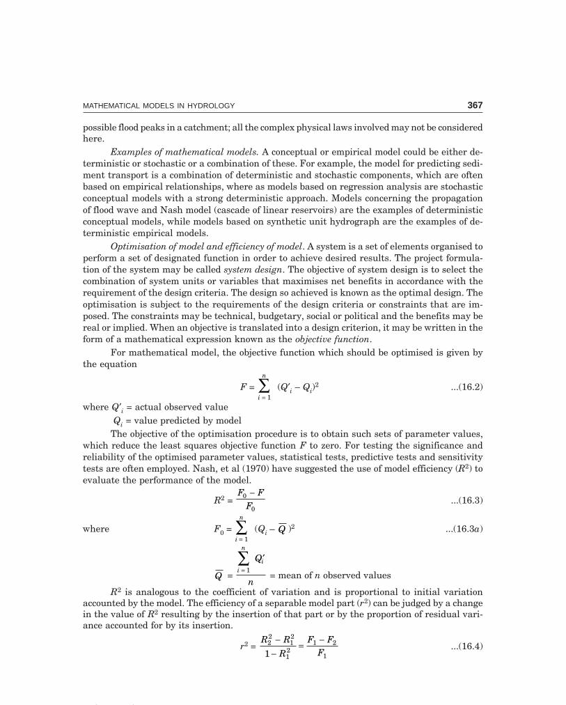
C-9\N-HYDRO\HYD16-1.PM5 367
MATHEMATICAL MODELS IN HYDROLOGY 367
possible flood peaks in a catchment; all the complex physical laws involved may not be consideredhere.
Examples of mathematical models. A conceptual or empirical model could be either de-terministic or stochastic or a combination of these. For example, the model for predicting sedi-ment transport is a combination of deterministic and stochastic components, which are oftenbased on empirical relationships, where as models based on regression analysis are stochasticconceptual models with a strong deterministic approach. Models concerning the propagationof flood wave and Nash model (cascade of linear reservoirs) are the examples of deterministicconceptual models, while models based on synthetic unit hydrograph are the examples of de-terministic empirical models.
Optimisation of model and efficiency of model. A system is a set of elements organised toperform a set of designated function in order to achieve desired results. The project formula-tion of the system may be called system design. The objective of system design is to select thecombination of system units or variables that maximises net benefits in accordance with therequirement of the design criteria. The design so achieved is known as the optimal design. Theoptimisation is subject to the requirements of the design criteria or constraints that are im-posed. The constraints may be technical, budgetary, social or political and the benefits may bereal or implied. When an objective is translated into a design criterion, it may be written in theform of a mathematical expression known as the objective function.
For mathematical model, the objective function which should be optimised is given bythe equation
F = i
n
=∑
1 (Q′i – Qi)
2 ...(16.2)
where Q′i = actual observed value Qi = value predicted by modelThe objective of the optimisation procedure is to obtain such sets of parameter values,
which reduce the least squares objective function F to zero. For testing the significance andreliability of the optimised parameter values, statistical tests, predictive tests and sensitivitytests are often employed. Nash, et al (1970) have suggested the use of model efficiency (R2) toevaluate the performance of the model.
R2 = F F
F0
0
−...(16.3)
where F0 = i
n
=∑
1 (Qi – Q )2 ...(16.3a)
Q = i
n
iQ
n=∑ ′
1 = mean of n observed values
R2 is analogous to the coefficient of variation and is proportional to initial variationaccounted by the model. The efficiency of a separable model part (r2) can be judged by a changein the value of R2 resulting by the insertion of that part or by the proportion of residual vari-ance accounted for by its insertion.
r2 = R R
R
F FF
22
12
12
1 2
11
−−
=−
...(16.4)
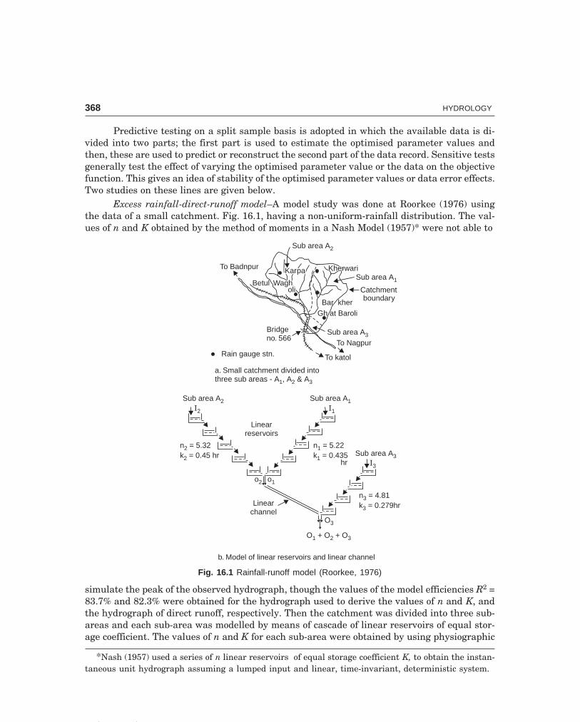
C-9\N-HYDRO\HYD16-1.PM5 368
368 HYDROLOGY
Predictive testing on a split sample basis is adopted in which the available data is di-vided into two parts; the first part is used to estimate the optimised parameter values andthen, these are used to predict or reconstruct the second part of the data record. Sensitive testsgenerally test the effect of varying the optimised parameter value or the data on the objectivefunction. This gives an idea of stability of the optimised parameter values or data error effects.Two studies on these lines are given below.
Excess rainfall-direct-runoff model–A model study was done at Roorkee (1976) usingthe data of a small catchment. Fig. 16.1, having a non-uniform-rainfall distribution. The val-ues of n and K obtained by the method of moments in a Nash Model (1957)* were not able to
Bridgeno. 566
To katol
To NagpurSub area A3
Sub area A1
CatchmentboundaryBar kher
Gh at Baroli
KherwariKherwari
Sub area A2
KarpaKarpa
Wagholi
Wagholi
Betul
To Badnpur
Rain gauge stn.
a. Small catchment divided intothree sub areas - A , A & A1 2 3
Sub area A2 Sub area A1I2 I1
Linearreservoirs
n = 5.322k = 0.45 hr2
n = 5.221k = 0.435
hr1
Sub area A3
Linearchannel
o1o2
I3
O3
O + O + O2 31
n = 4.813k = 0.279hr3
b. Model of linear reservoirs and linear channel
Fig. 16.1 Rainfall-runoff model (Roorkee, 1976)
simulate the peak of the observed hydrograph, though the values of the model efficiencies R2 =83.7% and 82.3% were obtained for the hydrograph used to derive the values of n and K, andthe hydrograph of direct runoff, respectively. Then the catchment was divided into three sub-areas and each sub-area was modelled by means of cascade of linear reservoirs of equal stor-age coefficient. The values of n and K for each sub-area were obtained by using physiographic
*Nash (1957) used a series of n linear reservoirs of equal storage coefficient K, to obtain the instan-taneous unit hydrograph assuming a lumped input and linear, time-invariant, deterministic system.

C-9\N-HYDRO\HYD16-1.PM5 369
MATHEMATICAL MODELS IN HYDROLOGY 369
features of the catchment. The outflow from sub-areas A1 and A2 was combined together andthen led through a linear channel having a translation constant T; it was then combined withoutflow of sub-area A3 to obtain the values of direct runoff for the whole catchment. The modelefficiency R2 = 82.3% and 90% for the first and second hydrographs, respectively. However,further analysis had to be made for investing the effect of loss assumptions and non-uniformrainfall distribution, and possibly inclusion of translation concept by dividing the sub-areas bymeans of isochrones and representing them by combination of linear channel and linear reser-voir in series.
Rainfall-runoff model based on retention concept. The retention concept of dividing therainfall into runoff and non-runoff volumes is based on the physical processes of soil moistureretention. Model based on the retention concept was used by Seth (1972) for simulating therainfall-runoff process of a small catchment. Its main components were those used to representthe retention capacity Y and evapotranspiration capacity E. Retention storage S was definedas that volume of water present in a natural watershed, which is not runoff storage. Themaximum storage volume V of the retention storage of the catchment was subdivided into V1and V2 for the upper and lower layer of soil, respectively. The moisture storage at any time,i.e., retention storage in the upper and lower layers were S1 and S2, respectively, and the ratioof S1/V1 and S2/V2 characterised the moisture status of the upper and lower layers, respectively
V = V1 + V2 ...(16.5)S = S1 + S2 ...(16.5a)
Precipitation
Rainfallexcess (Pnet)Rainfallexcess (Pnet)
Infiltration (F)Infiltration (F) Other abstractionsOther abstractions
Subsurfaceflow
Subsurfaceflow
Deeppercolation
Deeppercolation
Ground waterGround water
DelayedinterflowDelayedinterflow
PromptinterflowPromptinterflow
Direct surfacerunoff, DSR(Q )d
Direct surfacerunoff, DSR(Q )d
Base flow (BF)Base flow (BF)
Total runoff(TR or Q)
Total runoff(TR or Q)
Fig. 16.2 Rainfall-runoff system
These components together with other components of the model gave a good perform-ance when about a year’s data of 2560 data pieces of 3 hourly values of rainfall, runoff andpotential evaporation of Grendon Underwood Catchment of Institute of Hydrology (UK), wereused. The values of F = 14.07 mm2 and R2 = 0.912 obtained after optimisation run, comparedquite favourably with those obtained by using the Stanford Model for the same data. Themodel values of soil moisture retained in soil gave almost a similar pattern as the observed soil

C-9\N-HYDRO\HYD16-1.PM5 370
370 HYDROLOGY
moisture. However, to take into account the full range of seasonal variations, it would bedesirable to include a wide range of antecedent and storm period conditions existing perhapsover several years.
Rainfall-runoff system model. The rainfall to runoff transformation as a system is shownin Fig. 16.2.
A famous computer model is the Stanford Watershed Model (Crawford and Linsley,1966). This model is refined progressively and is now a very comprehensive model based onwater budgeting. By using hourly precipitation data and daily evapotranspiration as the maininputs, the model is programmed to produce hourly streamflow. Soil, vegetation, land use,etc., are all accounted for by a set of parameters, the values for which are progressively optimisedby search technique. The flow diagram for the model is shown in Fig. 16.3 a which is, typicalflow chart for a rainfall-runoff model of the explicit soil moisture accounting type, ESMA,redrawn from Linsley and Crawford (1974).
KEY
Input
Output
Storage
Functions
Precipitation potenialevapotranspiration
temperatureradiation
Snow melt
Interception
Imperviousarea
Infiltration
Inter-ceptionstorage
Evapo-transpi-ration
Actualevapotranspiration
Evapo-transpi-ration
Evapo-transpi-ration
Evapo-transpi-ration
Deep orinactive groundwater storage
Ground-water
storage
Active ordeep groundwater storage
Simulatedstreamflow
Channelouting
Channelinflow
Lowerzone
storage
Lower zone orground water
storageUpperzone
depletion
Upperzone
storage
Upperzone
Surfacerunoff
interflow
Upperzone
depletion
Over-landflow
Channel
inflow
Channel
inflow
Channel
inflow
Fig. 16.3 Flow diagram of stanford watershed Model IV, ESMA(after Linsley and Crawford, 1974)

C-9\N-HYDRO\HYD16-1.PM5 371
MATHEMATICAL MODELS IN HYDROLOGY 371
16.2 METHODS OF DETERMINING IUH
1. By the S-Curve HydrographIn Fig. 16.4, St is the S-curve ordinate at any time t (due to tr-hr UG) and S′t is the ordinate attime t of the S-curve lagged by t′r-hr, then the t′r-hr UGO at time t can be expressed as
U(t′r, t) = (St – S ′t ) ttr
r′...(16.6)
dt
dStdSt
St¢St¢
StSt
t¢rt¢rLag
tTime (hr)
Lim (S - S ) = d St 0
t t tr
¢¢
( UHO) = = Slope ofS - Curve
I td Sdt
t
Dis
char
ge(c
umec
)
Fig. 16.4 IUH as S-curve derivative
As t′r progressively diminishes, i.e., t′r → 0, Eq. (16.6) reduces to the form (as can be seenfrom Fig. 16.4)
U(0, t) = dSdt
t ...(16.7)
i.e., the ordinate of the IUH at any time t is simply given by the slope of the S-curve at time t;in other words, the S-curve is an integral curve of the IUH. Since the S-curve derived from theobserved rainfall-runoff data can not be too exact, the IUH derived from the S-curve is onlyapproximate. The IUH, reflects all the catchment characteristics such as length, shape, slope,etc., independent of the duration of rainfall, thereby eliminating one variable in hydrographanalysis. Hence, it is useful for theoretical investigations on the rainfall-runoff relationshipsof drainage basins. The determination of the IUH is analytically more tedious than that of UGbut it can be simplified by using electronic computers.
The t′r-UGO can be obtained by dividing the IUH into t′r-hr time intervals, the average ofthe ordinates at the beginning and end of each interval being plotted at the end of the interval(Fig. 16.5).

C-9\N-HYDRO\HYD16-1.PM5 372
372 HYDROLOGY
A
B
C
D
E D + E2
t –hr UG¢r
IUH derivedfrom S-curve
C + D2
B + C2
A + B2
Dis
char
ge(c
umec
)
Time (hr)tr¢ tr¢ tr¢ tr¢
Fig. 16.5 tr′-hr UG derived from IUH
2. By Using a Convolution IntegralBy the principle of superposition in the linear-unit-hydrograph theory, when a net rainfall offunction i(t) of duration t0 is applied, each infinitesimal element of Pnet will produce a DRO,i.e., Q(t) given by
Q(t) = 0
tu t i d′z −( ) . ( )τ τ τ ...(16.8)
the upper limit t′ given by t′ = t, when t ≤ t0
t′ = t0, when t ≥ t0
Eq. (16.8) is called the convolution integral (or Duhamel integral) in which u (t – τ) is akernel function, i(τ) is the input function.
The shape of the IUH in Fig. 16.6 resembles a single peaked hydrograph. If the rainfalland runoff in the convolution integral are measured in the same units, the ordinates of the
IUH have the dimension 1
time .
The properties of the IUH are given by0 ≤ u(t) ≤ a positive peak value, for t > 0
u(t) = 0 for t ≤ 0u(t) → 0 for t → ∞ ...(16.9)
0
∞z u(t)dt = 1.0 and0
∞z u(t) dt = ti
where ti = lag time of IUH = time interval between the centroid of Pnet and that of direct runoff.See next chapter 17 on IUH.

C-9\N-HYDRO\HYD16-1.PM5 373
MATHEMATICAL MODELS IN HYDROLOGY 373
a.
b.
c.
Q(t)
Ott time t
Run-offhydrograph
Q(t) = u (t – ).i( ) dt t to
t¢
t = t, when t t¢ £ o
t = t , when t > t¢ o o
time t
u (t – )t
IUH
t – tt – tO
u(t
–)t
Otime t
Rainfallintensity
i( )ti( )t
tt dtt0t0
u( )t
Fig. 16.6 Convolution of i(τ) and IUH
3. By Conceptual ModelsVarious conceptual models have been proposed to develop the IUH. They may be of physicalanalogy or mathematical simulation composed of linear reservoirs, linear channels, or time-area diagrams.(a) Linear Reservoirs
A mathematical simulation of a drainage basin consisting of a series of linear reservoirsas proposed by J.E. Nash (1957) is discussed below:
A linear reservoir is a fictitious reservoir in which the storage is directly proportional tooutflow, i.e., S = KO.
From the principle of continuity
I – O = dsdt
...(16.10)
From the condition O = 0 when t = 0, and that S = KO, O = I(1 – e–t/k) ...(16.11)
when t = ∞, O = I, i.e., the outflow approaches an equilibrium condition and equals inflow. Ifthe inflow terminates at time t0 since outflow began, a similar derivation gives the outflow attime t in terms of out flow O0 at t0, as
Ot = O0 et t K− −( )/0 ...(16.12)
C-9\N-HYDRO\HYD16-1.PM5 374
374 HYDROLOGY
For an instantaneous inflow, which fills the reservoir storage S in time t0 = 0, and since
S = KO, O0 = SK
, hence from Eq. (16.12)
Oi = SK
e–t/K ...(16.13)
For a unit input or S = 1, the IUH of the linear reservoir is given by
u(t) = 1K
e–t/K ...(16.14)
This is represented by the hydrograph for the outflow from the first reservoir as shownin Fig. 16.7.
O1
O1
O3
O4
On
On – 1
I
Linear storagereservoirs
Q1
t
Q2
t
Q3
t
Qn
t
Q4
Qn–1
Hydrographs(O = Q )ii
Fig. 16.7 Routing through linear reservoirs (Nash’s Model)
(b) Simulation of Linear ChannelsA linear channel is a fictitious channel in which the time T required to translate a
discharge Q of any magnitude through a given channel reach of length x is constant. Hence,when an inflow hydrograph is routed through the channel, its shape will not change. At agiven section, the relation between the water area A and the discharge Q is linear (assumingvelocity to be constant), i.e.,
A = CQ
where C = f(T) called ‘translation coefficient’ which is constant at a given section.If a segment of inflow of duration ∆t and volume S is routed through a linear channel,
Fig. 16.8, the outflow is given byO = S δ(t, ∆t) ...(16.15)
where δ(t, ∆t) = 1∆t
...(16.16)
for 0 ≤ τ ≤ ∆ t and t = τ + T; it is zero otherwise, where τ is the time measured from the beginningof the segment. Eq. (16.16) is a ‘pulse function’. When ∆t → 0, this equation becomes an ‘im-pulse function’ δ(t), known as a ‘Dirac-delta function’, which represents the IUH for the linearchannel.

C-9\N-HYDRO\HYD16-1.PM5 375
MATHEMATICAL MODELS IN HYDROLOGY 375
I=
f(t)
O=
f(t–
)t
Dis
char
ge
Inflow hydrograph(segment)
Outflow hydrograph(segment)
time tDtDttt
TTtt
ttDtDt
Fig. 16.8 Routing through linear channel
4. Routing Time–Area Curve of BasinsThe principles of flood-routing can be used to derive unit hydrographs for a catchment wherethere are no complete records of rainfall-runoff.
The catchment may be divided into a series of sub-areas, each contributing inflow intodrainage channels (which have storage) due to a flash storm. The IUH can be divided into twoparts—the first representing inflow of the rain, and second, the gradual withdrawal from thecatchment storage, the dividing line being the inflection point on the recession limb, Fig. 16.9.
titi
Short rain
Inflectionpoint
Inflowof rain
Withdrawalfrom storage
Base flow
Time (hr)
Dis
char
ge,(
cum
ec)
Fig. 16.9 Hydrograph from short rain (IUH)
Assuming that the catchment discharge (O) and the storage (S) are directly propor-tional
S = KO ...(16.17)where K = storage coefficient.
From the principle of continuity, if I = inflow resulting from the instantaneous rain (I – O) ∆t = ∆S ...(16.18)

C-9\N-HYDRO\HYD16-1.PM5 376
376 HYDROLOGY
orI I1 2
2+
t – O O1 2
2+
t = S2 – S1 ...(16.19)
and S1 = KO1, S2 = KO2
and hence, O2 = C0I2 + C1I1 + C2O1 ...(16.20)
where C0 = 0 5
0 5.
.t
K t+ , C1 =
0 50 5
..t
K t+ , C2 =
K tK t
−+
0 50 5..
...(16.20a)
which are same as Eqs. (9.12 a, b, c) with Muskingum approach, putting x = 0.and when a sub-area distribution or time-area graph is used and I1 = I2, hence
O2 = C′I + C2O1 ...(16.21)
where C′ = t
K t+ 0 5. , C′ + C2 = 1
From Eq. (16.18), I – O = dSdt
� S = KO,dSdt
= K dOdt
∴ K dOdt
= I – O
Using the condition O = 0, when t = 0, the equation can be solved as O = I(1 – exp (– t/K )) ...(16.22)
Since the inflow ceases at the inflection point at time ti, the outflow at time t (in termsof the outflow Oti at ti) is given by
Qt = Oti exp −−F
HGIKJ
t tK
i
Storage coefficient K can be determined from an observed hydrograph by noting twovalues of O, unit time apart at the point of inflection (Fig. 16.10).
A
1
ti
Directrunoff
time (t)O
Dis
char
ge,c
umec
A = K (O – O )1 2
Inflexion point
O = O1 ti
O = O2 ti + 1
O = Ot ti
t – tK
i–
Fig. 16.10 Determination of storage coefficient
O1 = Oti and O2 = Oti exp −−F
HGIKJ
t tK
i

C-9\N-HYDRO\HYD16-1.PM5 377
MATHEMATICAL MODELS IN HYDROLOGY 377
the shaded area A = t
t
i
i +z 1 Oti exp −
−FHG
IKJ
t tK
i = – KOti exp −−F
HGIKJOQP
t tK
i
0
1
= KOti – Oti exp −FHGIKJ
1K
∴ A = K(O1 – O2) ...(16.23)Another observation that is to be made is the catchment lag (ti), i.e., the maximum
travel time through the catchment. This may be taken as the time from the mass centre of thecausative rain (flash storm or short rainburst to minimise error) to the inflection point on therecession limb.
The catchment is subdivided into isochrone such that the rain falling in any sub-areahas the same time of travel to the outflow point O, (Fig. 16.11). The time-area graph (I) nowhas instantaneous unit rain applied to it and is routed through to obtain the outflow (O), Eq.(16.21). This outflow represents the IUH for the catchment and may be converted, if requiredto a tr-hr unit hydrograph.
1
2
3
45 6
78
9
IsochronesCatchment boundary
A = 1040 km2
t = 9 hrK = 8 hr
i
0
Fig. 16.11 Catchment divided into isochrones
This method is simple and the design rain can be applied directly to the time-area graph,with areal variation and with any desired intensity.
An estimate of K can also be had from data on the recession limbs of the basinhydrographs.Example 16.1 A catchment of area 1040 km2 is divided into 9-hourly divisions by isochrones(lines of equal travel time) in Fig. 16.11. From the observation of a hydrograph due to a shortrain on the catchment, ti = 9 hr and K = 8 hr. Derive: (a) the IUH for the catchment. (b) a 3-hrUG.Solution (i) It will be assumed that the catchment is divided into sub-areas such that allsurface runoff from each of these areas will arrive during a 1-hr period at the gauging point.The areas are measured by planimetering each of the hourly areas as:
Hour: 1 2 3 4 5 6 7 8 9Area (km2): 40 100 150 180 160 155 140 80 35(ii) The time-area graph (in full lines) and the distribution graph of runoff (in dotted
lines) are drawn as shown in Fig. 16.12. The dotted lines depict the non-uniform areal distri-bution of rain.

C-9\N-HYDRO\HYD16-1.PM5 378
378 HYDROLOGY
× 0.882
× 0.882× 0.882
0 1 2 3 4 5 6 7 8 9
200
180
160
140
120
100
80
60
40
20
0
Time (hr)
Are
a,(k
m2 )
Fig. 16.12 Time-area graph for catchment
Table 16.1 IUH by routing and derivation of 3-hr UG (Example 16.1)
Time Time-area 0.1177 I = 2.78 0.882 × col (5) O2 = IUH 3-hr UGO(hr) diagram × 0.1177 previous (cumec) = col (3) (cumec)
Area (km2) × col (2) (cumec) + col (4)(cumec)
1 2 3 4 5 6
0 0 0 0 0 0
1 40 13.1 0 13.10
2 100 32.7 11.54 44.24
3 150 49.1 39.00 88.10 44.00
4 180 58.9 77.70 136.60
5 160 52.3 120.40 172.70
6 155 50.7 152.00 202.70 145.40
7 140 45.8 179.00 224.80
8 80 26.2 197.00 223.20
9 35 11.4 196.50 208.00 205.30
10 0 0 184.50 184.50
11 0 0 163.70 163.70
12 0 0 145.00 145.00 176.50
13 0 0 128.60 128.60
14 0 0 114.00 114.00
15 0 0 101.00 101.00 123.00
Plot col (1) vs. col (5) to get the IUH, and col (1) vs. col (6) to get the 3-hr UGO, as shownin Fig. 16.13.

C-9\N-HYDRO\HYD16-1.PM5 379
MATHEMATICAL MODELS IN HYDROLOGY 379
(iii) From Eq. (16. 21), O2 = C′I + C2O1
C′ = t
K t+ 0 5. =
18 0 5 1
18 5+ ×
=. .
= 0.1177
C2 = K tK t
−+
= − ×+ ×
=0.50.5
8 0.5 18 0.5 1
7.55
= 0.882, Check: C′ + C2 = 1
Hence, the routing equation becomesO2 = 0.1177 I + 0.882 O1
O2 vs. time gives the required synthetic IUH from which the 3-hr UGO are obtained ascomputed in Table 16.1. The conversion constant for Col (3) is computed as
1-cm rain on 1 km2 in 1 hr = 10 10
3600
6 2× − = 2.78 m3/s
The 3-hr UGO is obtained by averaging the pair of IUH ordinates at 3-hr intervals andwriting at the end of the intervals.
0 1 2 3 4 5 6 7 8 9 10 11 12 13 14 15 16Time (hr)
240
220
200
180
160
140
120
100
80
60
40
20
0
3-hr UG (byaveraging IUHO)
IUHderived
Dis
char
ge(c
umec
)
Fig. 16.13 IUH derived and 3-hr UG (Example 16.1)
16.3 SYNTHETIC STREAM FLOW
The probability of occurrence of floods or droughts are more severe than that observed fromthe available stream flow records has to be known. On the assumption that the streamflow isessentially a random variable, it is possible to develop a synthetic flow record by statisticalmethods.
It has been found that high flows are likely to follow high flows and the low flows followlow flows, i.e., any event is dependent on the preceding event. This persistence is measured by

C-9\N-HYDRO\HYD16-1.PM5 380
380 HYDROLOGY
a serial lag coefficient. The lag interval may be one or several time units. A simple one lagMarkov generating equation for annual flows Q is
Qi = Q + ri(Qi–1 – Q ) + εiσ 1 2− ri ...(16.24)
where σ = standard deviation of Q
Q = mean of Q
i = 1 year to n year (flows in series)ri = lag-1 Markov coefficient, which is a portion of the departure from the previous flow
from the mean.The Eq. (16.25) yields a normal synthetic flow that preserves the maximum variance,
and first-order-correlation coefficient of the observed record. Statistical streamflow modelsare assumed stationary, i.e., the mean and variance of the observations (time series) are un-changed with time.
Thomas and Fiering (1962) used the Markov Chain model for generating monthly flows(by serial correlation of monthly flows) by using the following recursion equation.
qi+1 = qj + 1 + bj (qi – q j ) + εi σj+1 1 2− rj ...(16.25)
where qi, qi + 1 = discharges in the i and i + 1 months, respectively
q j , qi +1 = mean monthly discharges in the j and j + 1 months of the annual cycle
bj = regression coefficient for estimating the discharge in the j + 1 month fromthat in the j month
εi = a random normal deviate at time i with a zero mean and unit variance. σj + 1 = standard deviation of discharges in the j + 1 month rj = correlation coefficient between the discharges in the j and j + 1 months.The Eq. (16.25) is called ‘Lag-one single period Markov Chain Model, where the period
may be day, month or year.To reflect different seasonal or monthly means, the multi-period Markov model is used,
which requires a double indexing subscript as (using Q for annual flows)
Qi, j = Qj + bj (Qi–1, j–1 – Qj−1) + εi σj 1 2− rj ...(16.26)
where bj = rj σ
σj
j−
FHG
IKJ1
, since Qj+1 ≠ Qj ...(16.26a)
j = number of seasonal periods or months in the year and other terms have been definedin Eq. (16.25) in which q = Q for annual flows.
This model has been used extensively in stream flow analysis. The single-and multi-period Markov generation procedures sometimes result in negative flows. These flows must beretained for generating the next flows in sequence and then they may be discarded.
The procedure assumes that the discharges (or their transform) are normally distrib-uted. A synthetic flow record generated like this can be of any desired length and may wellinclude flow sequences more critical than any in the available observed record. Stochasticanalysis can be used to generate a number of synthetic-flow traces of length equal to the ex-pected useful life of project under study.

C-9\N-HYDRO\HYD16-1.PM5 381
MATHEMATICAL MODELS IN HYDROLOGY 381
Stochastic methods may be employed to generate a synthetic record of rainfall, whichcould be transformed to streamflow (by doing a particular operation), which the availablestreamflow records are found too short for a stochastic generation. The Markov process forgenerating a sequence of rainfall data is given by the relation
P (Xt + 1 = j|Xt = i) . ..(16.26b)which expresses the conditional probability of ‘transitioning’ from the state i at period t tostate j at (t + 1).
Matalas (1967) used a simple matrix representation of the problem, similar to theMarkovian model, as
Xt + 1 = AXt + Bεt + 1 ...(16.27)where Xt = n × 1 matrix representing the non-autocorrelated standardised flow at n stationsat time t
Xt + 1 = a similar matrix as above at time (t + 1)εt + 1 = n × 1 matrix of non-autocorrelated random numbers with zero mean and unit
varianceA, B = n × n matrices, the elements being so chosen as to preserve time mean q , vari-
ance σ2, lag 1-serial correlation coefficient r and the cross correlation coefficients rnm betweenall the data elements being modelled.
Data generated by models can be used to design reservoir capacity by using low-flow-frequency mass diagram and other techniques. Several hundred years of records are gener-ated to obtain an adequate number of high-and low-flow sequences.
16.4 FLOW AT UNGAUGED SITES BY MULTIPLE REGRESSION
At sites where streamflow records are not available, the flow can be estimated by a multiple-regression technique using the drainage basin and climatic characteristics as independentvariables. The regression constant and coefficient are calculated using streamflow data fromgauged streams. By expressing the variables in common logarithms, the equation can be trans-formed to the linear form as
log Q = a + b1 log x1 + b2 log x2 + ... + bn log xn ...(16.28)where Q = annual or monthly peak flow or runoff volume with any assigned probability andduration; the dependent variable, cumec.
a = regression constantx = an independent variable characteristic of a drainage basin or its climatic factorb = the regression coefficient for xTwenty or more sets of data are required to obtain reliable values of the regression
constant and coefficients by solving Eq. (16.28), which is usually done by the use of a computer.
16.5 RESERVOIR MASS CURVE
A mass curve (or Rippl diagram, 1882) is a cumulative plotting of net reservoir inflow (Fig. 16.14),and is expressed as
V(t) = 0
tz Q(t)dt ...(16.29)

C-9\N-HYDRO\HYD16-1.PM5 382
382 HYDROLOGY
where V(t) = volume of runoff Q(t) = reservoir inflow
both as functions of time
D
C
Ave. rateof flow = X
t – t2 1XX
V = shaded area abovetV = shaded area abovet
b. Flow mass curve(Rippl’s curve, 1882)
b. Flow mass curve(Rippl’s curve, 1882) Rotate AB
to horizontalfor ‘residualmass curve’
t1 t2t Time t (hr)
Time t (hr)
VtVt
t
a. Hydrograph ofriver inflow
B
Dis
char
geQ
(cum
ec)
Cum
ulat
ive
inflo
wV
(ha-
m)
c. Residual mass curve Range R
Normal line BA–
+
Time t (hr)
Dep
artu
res
from
norm
al(h
a-m
)+
–
Fig. 16.14 Flow and residual mass curves
The instantaneous rate of flow at any point on the mass curve is given by the slope of thetangent at the point, i.e.
Q(t) = dV t
dt( )
...(16.29a)
As already discussed, the mass curve has many useful applications in the design of astorage reservoir, such as determination of reservoir capacity, operations procedure and floodrouting.

C-9\N-HYDRO\HYD16-2.PM5 383
MATHEMATICAL MODELS IN HYDROLOGY 383
16.6 RESIDUAL MASS CURVE
Instead of plotting a mass curve, the departure of the mass curve from the normal (AB) may beplotted against time. In other words, the mass curve is plotted about a horizontal axis obtainedby rotating the average slope line AB of the mass curve, to the horizontal (Fig. 16.14 (c)). Sucha plot is called a ‘residual mass curve’. This method of plotting saves the additional spaceneeded for plotting a continuously rising mass curve and to accentuate more clearly the crestsand troughs of the cumulative flow records.
The difference between the maximum and minimum values of a residual mass curve fora given period ‘n’ is known as the ‘range’ for the period ‘n’. If R is the range of a period of nyears of annual-runoff record-whose sample standard deviation is σ, then according to Hurst(1951, 1956) and Klemes (1974)
R = σ n k
2FHG
IKJ ...(16.30)
where k varies from 0.5 to 1 with an average value of 0.73. Here R will be the required storageif a steady discharge equal to the mean over a period of n years is to be produced. Theoreti-cally, it can be shown that if the runoff record is a normally distributed random time series,then
R = 1.25 σp n ...(16.31)where σp = the population standard deviation.
16.7 SELECTION OF RESERVOIR CAPACITY
The determination of the required capacity of a storage reservoir is usually called an ‘opera-tion study’ using a long-synthetic record. An operation study may be performed with annual,monthly, or daily time intervals; monthly data are most commonly used.
When the analysis involves lengthy synthetic data, a computer is used and a sequent-peak algorithm is commonly used. Values of the cumulative sum of inflow minus withdrawalstaking into account the precipitation, evaporation, seepage, water rights of the downstreamusers, etc., are calculated, (Fig. 16.15). The first peak and the next following peak, which isgreater than the first peak, i.e., the sequent, peak, are identified.
Time (months)
Sequent peaks
Maxstorage
MaxstorageStorageStorage
Initial peak
S(I
nflo
w–
Dem
and)
, (10
00ha
-m)
0
+ve
–ve
Fig. 16.15 Sequent-peak algorithm

C-9\N-HYDRO\HYD16-2.PM5 384
384 HYDROLOGY
The maximum difference between this sequent peak and the lowest trough during theperiod under study is taken as the required storage capacity of the reservoir.
Example 16.2 The mean monthly flow data for a proposed reservoir site are given be-low:
Month Jan. Feb. Mar. April May June
Mean monthly flow (cumec) 6 3 1 2 7 1
Month July. Aug. Sept. Oct. Nov. Dec.
Mean monthly flow (cumec) 27 29 30 27 31 15
Determine the average discharge that can be expected throughout the year. Draw theresidual mass curve and obtain an expression for the range as developed by Hurst on the basisof the monthly flow data.
Solution
Mean Monthly Cumulative Cumulative Residualmonthly flow volume mothly mean flow mass curve
Month flow, x (ha-m) inflow (ha-m) throughout (ha-m)(cumec) the year (ha-m)
1 2 3 4 5 6
Jan 6 1575 1575 3931 –2356
Feb 3 790 2365 7862 –5497
Mar 1 262 2627 11793 –9166
April 2 525 3152 15725 –12573
May 7 1840 4992 19656 –14664
June 1 262 5254 23587 –18333
July 27 7100 12354 27518 –15164
Aug 29 7750 20104 31450 –11346
Spet 30 7880 27984 35381 –7397
Oct 27 7100 35084 39312 –4228
Nov 31 8150 43234 43243 –0009
Dec 15 3940 47174 47174 0
n = 12 179 47174
x = 17912
= 15 cumec Mean flow (per month)
throughout the year47174
12= = 3931.2 ha-m
The average discharge that can be expected throughout the year
Q = 47174 10365 86400
4 3××
mS
= 15 cumec = x
The residual mass curve is plotted in Fig. 16.16 and the range, R = 18333 ha-m, whichis the storage capacity of the reservoir to maintain the mean flow of 15 cumec throughout theyear.
x: 6 3 1 2 7 1 27 29 30 27 31 15
x – x : –9 –12 –14 –13 –8 –14 12 14 15 12 16 0

C-9\N-HYDRO\HYD16-2.PM5 385
MATHEMATICAL MODELS IN HYDROLOGY 385
(x – x )2: 81 144 196 169 64 196 144 196 225 144 256 0
Σ (x – x )2 = 1815
σ = Σ( )x x
n−−
=−
2
1181512 1
= 12.84 cumec
Let R = σ n k
2FHG
IKJ
18333 × 104 = 12.84 (30.4 × 24 × 60 × 60) 122
FHG
IKJ
k
6k = 18333 103370 10
4
4
××
= 5.44
∴ k = 0.945
J F M A M J J A S O N D Months
Storage forQ = 15 cumecthroughout year
Residualmass curve
Range, R= 18333 ha-m =
6
4
2
0
2
4
6
8
10
12
14
16
18
20
(–)
(+)
Res
idua
lmas
sin
(100
0ha
-m)
Fig. 16.16 Residual mass curve (Example 16.2)
Thus, the expression for range (on the basis of 12 months data) is
R = σ n2
0.945FHG
IKJ ...(16.32)
Usually k varies from 0.5 to 1.0, the average value being 0.73. Usually, a number ofyears of observation are required.Example 16.3 Given in Table 16.2 (Col. 1, 2, 3, 5 and 6) are the monthly inflows during low-water period at the site of a proposed dam, the corresponding monthly precipitation and pan

C-9\N-HYDRO\HYD16-2.PM5 386
386 HYDROLOGY
evaporation at a nearby station, and the estimated monthly demand for water. Prior waterrights downstream require a special release of 6 cumec or the natural inflow, whichever is less.Assuming that only 24% of the rainfall on the land area to be flooded by the proposed reservoirhas reached the stream in the past, reservoir area as 6000 ha on an average, and a pan coefficientof 0.7, construct the sequent peak alogrithm and determine the required storage capacity of thereservoir.Solution Since 24% of the rainfall (P) is runoff, which is already included in the monthlyinflows into the reservoir, only 100 – 24 = 76% of the rainfall on the reservoir area is to beincluded. Reservoir evaporation = 0.7 × pan evaporation (EP). (0.76P – 0.7 Ep) values have tobe multiplied by the average reservoir area at the beginning and end of each month.
The monthly change in storage and cumulative storage (at the end of each month) areworked out in Table 16.2 and the sequent peak algorithm is drawn as shown in Fig. 16.17 andthe required storage capacity of the Reservoir (difference between the initial peak and thelowest trough in the interval) is 13045 ha-m, which is also indicated in the col. (10) of Table16.2. Actually this process has to be done for 4-5 consesecutive years and the difference be-tween the highest peak and the suceeding lowest trough gives the required storagecapacity to meet the specified demand. The required storage capacity is also equal to the sumof the negative quantities (ΣDeficit) in Col (8) of Table 16.2, which is less than the sum of thepositive quantities (ΣSurplus) col (8), thus ensuring the filler of the reservoir during mon-soons.
July A S O N D J F M A M June
= Reservoirstorage
13045ha-m
Trough
Peak
Time months
24
20
16
12
8
4
0
4
8
12
16
–ve
+ve
S(I
nflo
w–
Dem
and)
(100
0ha
-m)
Fig. 16.17 Sequent-peak Algorithm (Example 16.3)
16.8 FLOOD FORECASTING
With the operation of flood forecasting centres in India since 1969, heavy loss of life and suffer-ing of people are greatly minimised due to advance warning. In the country, there are 8 fore-casting centres with 25 sub-centres and more than 200 observation sites have been equippedwith wireless. In addition to this, rainfall data from 30 ordinary rain gauge stations and 50self-recording rain gauge stations are also collected to supplement the gauge and dischargedata.

C-9\N-HYDRO\HYD16-2.PM5 387
MATHEMATICAL MODELS IN HYDROLOGY 387
Tab
le 1
6.2
Ope
rati
on s
tudy
for
a s
tora
ge r
eser
voir
(E
xam
ple
16.3
) U V| | W| | U V| | | | W| | | |
Σ Surplus =22051 ha-m
Σ Deficit = 13045 ha-m
22051 – 9006
|← = 13045 ha-m →|
Mon
thM
ean
Mon
thly
Pre
cipi
Pan
Eva
-D
eman
dD
/s R
elea
seC
han
ge i
nC
um
ula
tive
Res
ervo
irm
onth
lyfl
owta
tion
,po
rati
on,
(ha-
m)
(ha-
m)
stor
age,
∆s
stor
age,
capa
city
flow
, Q
volu
me
P (
mm
)E
p (m
m)
(ha-
m)
Σ∆ s
(ha-
m)
(cu
mec
)(h
a-m
)=
(3)
+ (
4) –
(ha-
m)
(5)-
(6)-
(7)
12
34
56
78
91 0
July
2769
98†
135
155
650
1555
†+
4758
*47
58
Au
g.29
7257
175
7597
515
55+
5210
9968
Sep
t.30
7776
140
8012
0015
55+
5071
1503
9
Oct
.27
6998
2512
517
5015
55+
3282
1832
1
Nov
.31
8035
565
2500
1555
+37
3022
051
Dec
.15
3888
040
2500
1555
–335
2171
6
Jan
.6
1555
050
2500
1555
–271
019
006
Feb
.3
777
080
2400
777
–273
616
270
Mar
ch1
259
010
022
5025
9–2
670
1360
0
Apr
il2
518
2013
015
0051
8–1
955
1164
5
May
718
1445
195
1250
1555
–160
510
040
Jun
e1
259
100
200
650
259
–103
490
0613
045
1. †
27 c
um
ec ×
30
days
= 2
7(30
× 8
6400
)/10
4 =
6998
ha-
m2.
†56
cu
mec
× 3
0 da
ys =
6 (
30 ×
864
00)/
104
= 15
55 h
a-m
3. *
6998
+ 13
50.
7515
50.
710
00×
−×
× 6
000
– 65
0 –
1555
= +
4758
ha-
m
4. R
eser
voir
cap
acit
y =
sum
of
neg
ativ
e qu
anti
ties
in
col
. (8)
.

C-9\N-HYDRO\HYD16-2.PM5 388
388 HYDROLOGY
Factors governing forecasting can be divided into two groups—initial and final. Theinitial factors govern conditions existing at the time when the forecast is made and can beestimated on the basis of current hydrometeorological observations. The final factors includethe future weather conditions and has to be taken into account in hydrological forecasts, if anaccurate weather forecast is available. In practice, short-term forecasts of weather elementsare being used in compilation of hydrological forecasts and warnings.
The elements of forecasts include forecast of crest stages, discharge and time of occur-rence, etc. In some cases, the other basic water regime elements to be known are:
(i) volume of runoff in respect of various periods of time(ii) flow distribution
(iii) MWL in reservoir and the data of occurrenceThe data required for making an accurate forecast are:(a) stage and discharge of upstream base station(b) stage and discharge of forecasting station(c) change in stage and discharge of these stations(d) stage and discharge of any tributary joining the main stream between the base sta-
tion and forecasting site(e) the intensity, duration and distribution of rainfall in the main, intercepted or sub-
catchment(f) topography, nature of vegetation, soil type, land use, population density, depth of
GWT etc., of the main or intercepted catchment(g) the atmospheric and climatic conditions.The factors (a) to (d) are the basic parameters used in developing correlation curves or
mathematical models; factor (d) can be neglected if its contribution is not appreciable, andfactors (e) and (f) are taken into account for introducing rainfall and antecedent precipitationindex as additional parameters; however, (g) stands as a future factor.
The forecasing methods currently used in the country are:(a) based on laws governing the movement of water in the channel, i.e., using the hydro-
dynamic methods to determine the movement and transformation of flood waves(b) based on the analysis of hydrometerological data of the river basin, i.e., water balance
studies taking into account precipitation, the water equivalent of snow cover, soil moisture,ground water and other factors and estimating runoff, which require the use of a computer.
For small catchments, approximate calculations of flood movement and transformationcan be made by:
(i) multiple correlation between stage and discharge observations(ii) streamflow routing on river reaches
(iii) mathematical modelMultiple correlation has the advantage of using parameters like rainfall or antecedent
precipitation index. Streamflow routing method includes the effect of channel storage on theshape and movement of flood wave; Muskingum method is generally used. For example, therouting equation developed between Sikanderpur and Rossera on Burhi Gandak (Bihar) is

C-9\N-HYDRO\HYD16-2.PM5 389
MATHEMATICAL MODELS IN HYDROLOGY 389
O2 = 0.612I1 + 0.033I2 + 0.355O1 ...(16.33)where K = 36 hr, x = 0.3 and t = 24 hr
16.8 MATHEMATICAL MODEL
A linear reservoir attenuates the peak of an inflow hydrograph and a linear channel translatesinflow hydrograph in time, which are representative of the physical action performed by thecatchment. Hence, a model of a linear reservoir connected in series with a linear channel maybe selected in this study. A linear channel is defined by the delay time or the time of travel ofthe flood wave and is approximately determined with the help of time to peaks of flood eventson the upstream and downstream stations of a river reach. Muskingum equation defines thelinear reservoir by its storage-discharge relation as
S = K[xI + (1 – x)O] ...(16.34)From the principle of continuity
I – O = dSdt
or S2 – S1 = I I
tO O1 2 1 2
2 2+F
HGIKJ −
+FHG
IKJ t ...(16.35)
From Eq. (16.34) S1 = K[xI1 + (1 – x)O1] S2 = K[xI2 + (1 – x)O2]S2 – S1 = K[x(I2 – I1) – (1 – x)(O2 – O1)] ...(16.36)
From Eqs. (16.35) and (16.36), O2 = C0I2 + C1I1 + C2O1 ...(16.37)
where C0 = – Kx t
K Kx t−
− +0 5
0 5.
., C1 =
Kx tK Kx t
+− +
0 50 5
..
C2 = K Kx tK Kx t
− −− +
0 50 5..
...(16.37a)
and C0 + C1 + C2 = 1The routing period t (time interval between O1 and O2) should be equal to or less than
the time of travel through the reach.Eq. (16.37) for successive time intervals may be written as
O3 = C0I3 + C1I2 + C2O2 ...(16.38)O4 = C0I4 + C1I3 + C2O3 ...(16.39)
Eq. (16.38) – (16.37) gives:O3 – O2 = C0(I3 – I2) + C1(I2 – I1) + C2(O2 – O1) ...(16.40)
Eq. (16.39) – (16.38) gives:O4 – O3 = C0(I4 – I3) + C1(I3 – I2) + C2(O3 – O2) ...(16.41)
Assuming the stage (gauge height)—discharge curves as a straight line (as a first ap-proximation), if the slopes of the curve on upstream and downstream are 1/a and 1/b,Fig. 16.18 (a) then
I IH H
a2 1
2 1 1−−
= andI I
H Ha3 2
3 2 1−−
=

C-9\N-HYDRO\HYD16-2.PM5 390
390 HYDROLOGY
O OG G
b2 1
2 1 1−−
= andO OG G
b3 2
3 2 1−−
=
1a3
a21
1a1
Assumedratingcurve
Actualratingcurve
H – Upstream gauge
Inflow I (cumec)
Sta
geH
(m)
Outflow O (cumec)
Sta
geG
(m)
b1
1
b2
1
b31
Assumedrating curve
Actualrating curve
G – Downstream gauge
O1O2O3O4Outflow O (cumec)
G1
G2
G3
G4
Sta
ge(m
)
Assumedrating curve
G – Downstreamgauge
Actual ratingcurve
b1
G – G2 1
O – O2 1
1
b=
H – Upstream gauge
Actual ratingcurve Assumed
rating curve
Slope 1a
1aH
–I I2 1
2 1– H 1
a=
I1 I2 I3
H1
H2
H3
Inflow (cumec)I
Sta
ge(m
)
a. Stage – discharge rating curves assumed linear
b. Stage–discharge curves divided into three linear parts
Fig. 16.18 Stage-discharge-rating curves Assume
Substituting these in Eq. (16.40)b(G3 – G2) = C0a(H3 – H2) + C1a(H2 – H1) + C2b(G2 – G1)
or G3 – G2 = C2(G2 – G1) + C0
ab
(H3 – H2) + C1
ab
(H2 – H1) ...(16.42)
Similarly, substitution in Eq. (16.41) gives
G4 – G3 = C2(G3 – G2) + C0 ab
(H4 – H3) + C1 ab
(H3 – H2) ...(16.43)
Eqs. (16.42) and (16.43) may be written asG3 – G2 = x1(G2 – G1) + x2(H2 – H1) + x3(H3 – H2)G4 – G3 = x1(G3 – G2) + x2(H3 – H2) + x3(H4 – H3)
where x1 = C2, x2 = C1 ab
, and x3 = C0 ab
Thus, a number of equations can be obtained from the observed data and solved for x1,x2 and x3 by the least square technique. Since the number of such equations are very large,from large sets of data, a computer can be used. For example, the equations developed for astraight reach between Muzaffarpur and Rossera on Burhi-Gandak are
Rising stage:G3 – G2 = – 0.401 (G2 – G1) + 2.826 (H2 – H1) – 0.94 (H3 – H2) ...(16.44)

C-9\N-HYDRO\HYD16-2.PM5 391
MATHEMATICAL MODELS IN HYDROLOGY 391
Falling stage:G3 – G2 = – 0.1413(G2 – G1) + 0.3018(H2 – H1) + 0.6082(H3 – H2) ...(16.45)
As a further refinement the stage discharge curves may be divided into linear parts, saythree, and the slopes denoted according to the linear ranges in which the stages lie, as shownin Fig. 16.18 (b), and the equations solved by using multiple regression technique.
Contribution due to a major tributary between the base station and the forecastingstation has to be taken into account.
The results of flood routing between Sikanderpur (Muzaffarpur) and Rossera by differ-ent methods during the 1975 floods are given in Table 16.3 for comparison. It can be seen thatthe Muskingum method has given more consistent results. A clear picture of forecast andcomparison with past values have been found possible only in graphical correlation and minoradjustment based on experience can be done in the predicted value. These are not possible in themathematical model and also the model cannot give better results in rivers having large scalefluctuations due to existance of control structures, their operation or flashy nature of the stream.
Contribution due to TributaryContribution due to a major tributary between the base station and the forecasting station hasto be taken into account. For example, three major tributaries of Ganga affect the gauge down-stream at Patna, other than its own (Fig. 16.19).
Table 16.3 Comparison of flood forecast results
Date Time Level Level downstream (m)
(hr) upstream Date Time Graphi- Musk in- Mathe- Observed(m) (hr) cal cor- gum matical
relation method model
29.7.1975 08–00 42.298 30.7.1975 08–00 42.750 43.000 43.038 42.900
30.7.1975 08–00 42.903 31.7.1975 08–00 43.600 43.750 43.527 43.623
31.7.1975 08–00 43.583 01.8.1975 08–00 44.480 44.750 44.676 44.723
01.8.1975 08–00 44.773 02.8.1975 08–00 45.320 45.100 45.139 44.583*
*The large variation in the last observation is due to number of breaches in the embankmentbetween Muzaffarpur and Rossera.
Trib
utar
y1
Tributary2Tributary
3
River
Ganga
H¢I¢
I, HUpstream
I² ², H
I²¢, H²¢O, GDownstream
gauge (at Patna)
Fig. 16.19 Tributary effect on gauge downstream

C-9\N-HYDRO\HYD16-2.PM5 392
392 HYDROLOGY
In such a case, the modified Muskingum equation can be written asO2 = C2O1 + C1I1 + C1′I1′ + C1″I1″ + C1′″I1′″ + C0I2 + C0′I1′
+ C0″I2″ + C1′″C2′″ ...(16.46)Similarly, O3 can be written and O3 – O2 can be evaluated. Aproximating, its stage (gauge
height)-discharge curve, to a straight line, the ultimate equation will be of the form (writingG3 – G2 as G3.2 and so on)
G3.2 = x1G2.1 + x2H2.1 + x3H3.2 + x4H′2.1 + x5H′3.2 + x6H″2.1
+ x7H″3.2 + x8H″′2.1 + x9H″′3.2 ...(16.47)Number of equations have been formed like this from the observed data and solved for
the constants by the least square technique by using a computer. The constants obtained forthe forecasting site at Patna for the 1975 floods are given in Table 16.4, and the levels reachedin Table 16.5 (compared with values obtained by graphical correlation, which has given betterresults).
Table 16.4 Constants for forecasting site at Patna
Constant Rising stage Falling stage
x1 0.5393 0.2622
x2 0.1407 0.2783
x3 –0.0919 0.0575
x4 –0.1855 0.2783
x5 0.1132 0.0427
x6 –0.0608 0.0535
x7 –0.1271 –0.0361
x8 0.0080 –0.0196
x9 0.1192 +0.2002
Table 16.5 Flood forecast results at Patna during 1975
Date Time Level Level downstream (m)
(hr) upstream Date Time Graphical Mathe- Observed(m) (hr) correlation matical
model
22.8.1975 09–00 48.799 23.8.1975 09–00 49.429 49.299 49.449
23.8.1975 17–00 48.679 24.8.1975 17–00 49.929 50.089 49.969
24.8.1975 01–00 49.859 25.8.1975 01–00 49.929 55.089 49.989
09.9.1975 09–00 49.519 10.9.1975 09–00 48.809 48.774 48.794

17.1 IUH FOR A BASIN
An IUH is a direct-runoff hydrograph producing a unit rainfall excess (Pnet = 1 cm) precipitat-
ing instantaneously over the catchment; i.e., i = 1tr
, tr → 0; i increases and the UG becomes
more skewed, called IUH, Fig. 16.6 (b). The shape of the IUH resembles a single peakedhydrograph. The properties of the IUH are given by Eq. (16.9); and its time to the peak < timeto the centroid of the curve. The main advantage of IUH is that it eliminates the problem ofunit duration and restriction of uniform distribution of rainfall in time. It is independent ofthe duration of the rainfall excess (tr) and rainfall characterstics, and is indicative of the catch-ment storage characterstics (like length, shape, slope and storage coefficient), which makes iteminently suitable for theoretical analysis of rainfall-runoff relationship. The IUH is a uniquedemonstration of a particular catchment response to rain, i.e., ‘impulse response’. As the IUHis only an extension of the unit hydrograph concept, it is also based on the principles of liniarityand time invariance.
If the IUH of a basin is available, the application of Eq. (16.8) yields the direct runoffdue to any storm.
17.2 DERIVATION OF IUH
The IUH can be approximately derived from the S-curve, Eq. (16.7), i.e.,The ordinate of the IUH at any time t = tr × Slope of the S-curve derived from the tr–hr
UG at t, i.e.,
(IUHO)t = tr × ∆∆St t
FHG
IKJ ...(17.1)
The ordinate of the tr-hr UG at any time t = 1tr
× area of the IUH between (t – tr) and t
i.e., ut = 1tr
× ∆ At ...(17.2)
If the IUH is assumed linear between (t – tr) and t,
ut = ( )IUHOt
tr−2
...(17.3)
Chapter 17
393
INSTANTANEOUS UNIT HYDROGRAPH
(IUH)

C-9\N-HYDRO\HYD17-1.PM5 394
394 HYDROLOGY
i.e., average of IUHO at t and t – tr
which works well only when tr is small and the peak is not contained within the interval (t – tr)to t.
Eq. (17.3) can be used to derive a tr-hr UG from the available IUH, avoiding the con-struction of the S-curve hydrograph, see Fig. 16.5.
17.3 OTHER METHODS OF DERIVATION OF IUH
Many researchers have made extensive investigation on the derivation of unit hydrograph(UG) since Sherman gave the principle of UG in 1932.
The approaches utilised to develop linear conceptual models of rainfall-runoff relation-ship may be classified into three groups:
The first group employs a differential equation that supposedly governs the equation ofa specified system; input-output relation, with rainfall as input and runoff as output(Kulandia swamy, Chow–1964), see Eq. (16.1).
The second group utilises an arrangement of the so called conceptual elements in-cluding linear channels and linear reservoirs (Nash 1957), time-area diagrams (Clark 1945),and geomorphological characterstics (Rodriguez-Iturbe and Valdes, 1979).
The third group makes hypothesis about rainfall-runoff relationship more or less onintutive grounds (Lienhard).
The practical approaches of Nash and Clark are discussed here and other methods pro-posed by Dooge, Diskin, etc., are not considered here.
Considerable work has been reported in the literature on the non-linear unit hydrographtheory, which is beyond the scope of this book.
17.4 NASH CONCEPTUAL MODEL
Nash considered that the IUH can be obtained by routing the instantaneous inflow through acascade of linear channels (n numbers) with equal storage coefficient (Fig. 16.7). The out flowfrom the first reservoir is considered as inflow into the second reservoir, and so on. The outflowfrom the nth reservoir yields the IUH given by
u(t) = 1
k nΓ etk
tk
n− −FHG
IKJ
1
, Γn = (n – 1) ! ...(17.4)
The value of the parameter n, which is a shape parameter, is a measure of the catch-ment channel storage, which defines the shape of the IUH. A lower value of n yields a higherpeak of IUH because of less storage flow attenuating the peak flow; a higher value of n leads toa lower peak of IUH signifying higher storage for attenuating peak flow. The parameter K(delay time, hr), which is a scale parameter, represents the dynamics of rainfall-runoff proc-ess in the catchment. A smaller K-value reflects a lower time to peak of the runoff hydrographand a higher K-value reflects a long time to peak.
The two parameters n and k may be computed by making an analysis of the observedrainfall-runoff data on the catchment as follows:
The first moment of the IUH about the origin (t = 0): M1 = nk ...(17.5)The second moment of the IUH about the origin (t = 0):
M2 = n(n + 1) k2 ...(17.6)

C-9\N-HYDRO\HYD17-1.PM5 395
INSTANTANEOUS UNIT HYDROGRAPH (IUH) 395
By routing through the cascade of n-reservoirs, it can be shown thatMQ1 – MI1 = nk ...(17.7)MQ2 – MI2 = n(n + 1)k2 + 2nk MI1 ...(17.8)
where MQ1, MQ2 are the first and second moments of direct runoff about the origin.and MI1, MI2 are the first and second moments of the effective rainfall (rainfall excess Pnet)about the origin.
The parameters n and k may be evaluated by solving these two equations as illustratedin the Example 17.1. Making use of these two parameters an IUH can be derived for a catch-ment of area eq. A km2; and also a tr-hr UG, as illustrated in Example 17.2; i.e., from theavailable rainfall-runoff data on a catchment of area A, and IUH and a tr-hr UG can be de-rived, for which the procedure involves the steps of both the Examples, 17.1 and 17.2.Example 17.1 The effective rainfall due to a 4-hr storm in the successive hours are: 2.6, 2.5, 2.3and 2.4 cm. The resulting DRO’s in the successive hours are: 3, 15, 26, 40, 50, 35, 25, 20, 15, 10,7, 4, 3 and 1 cumec. Determine the values of n and k.SolutionStep 1 Evaluate the first and second moments of Pnet about the origin, i.e., t = 0 (commence-ment of Pnet and DRO)
MI1 = 2 6 0 5 2 5 15 2 3 2 5 2 4 3 5
2 6 2 5 2 3 2 4. . . . . . . .
. . . .× + × + × + ×
+ + + = 19.2 cm . hr
9.8 cm ~− 2 hr
MI2 = 2 6 0 5 2 5 15 2 3 2 5 2 4 3 59 8
2 2 2 2. . . . . . . ..
× + × + × + × = 49.75 cm . hr
9.8 cm
2
~_ 5 hr2
Step 2 Evaluate the first and second moments of Qi about the origin;
Qi = DROi, Qt = ΣQ1 t1, MQ1 = t = Σ Q t
Q1 1 , Q = ΣQ1 = ΣDRO
Similarly, Qt 2 = ΣQ1t12; MQ2 = t 2 =
Σ Q tQ1 1
2
Table 17.1 To evaluate MQ1 and MQ2
Time DROt (hr) (cumec) Q × t Q × t2
(given) = Q (cumec-hr) (cumec-hr2)
0 0 0 01 3 3 32 15 30 603 26 78 2344 40 160 6405 50 250 12506 35 210 12607 25 175 12258 20 160 12809 15 135 1215
10 10 100 1000
(Contd.)...
C-9\N-HYDRO\HYD17-1.PM5 396
396 HYDROLOGY
(Contd.)...
11 7 77 847
12 4 48 576
13 3 39 507
14 1 14 196
15 0 0 0
ΣQ = 254 ΣQt = 1472 ΣQt2 = 102.93
MQ1 = t = 1472254
= 5.8 hr, MQ2 = t 2 = 10293254
= 40.5 hr2
Eq. (17.7): nk = MQ1 – MI1 = 5.8 – 2 = 3.8 hrEq. (17.8): MQ2 – MI2 = n(n + 1)k2 + 2 nk MI1
40.5 – 5 = nk2 (n + 1) + 2 × 3.8 × 2 35.5 = n2k2 + nk2 + 15.2
nk2 = 35.5 – 15.2 – (3.8)2 = 5.87
k = nknk
2 5 873 8
= ..
= 1.55
n = nkk
= 3 8155
..
= 2.45 ~_ 2 (whole number)
Example 17.2 Derive an IUH and a 2-hr UG (UGO at 2-hr intervals) for a catchment of 240km2, having n = 3 and k = 5 hr.Solution NASH Model, Eq. (17.4):
u(t) = 1 1
k ne
tk
tk
n
Γ. .
− −FHG
IKJ
k = 5 hr, n = 3 and Γn = (n – 1) ! = (3 – 1) ! = 2 ! = 2 × 1 = 2
u(t) = 1
5 2 55
3 1
×FHG
IKJ
− −
. .et
t
= 1
10 55
2
ett− F
HGIKJ
/
Table 17.2 IUHO and 2-hr UGO computation
Time IUHO
t(hr) t5
et5
− t5
2FHG
IKJ u(t) u(t) 2-hr UGO
(cm/hr) (cumec) (cumec)
= (3) (4)
10×
(5) × 2.78 × 240 (by averaging)
= (5) × 668
1 2 3 4 5 6 7
0 0 1 0 0 0 0
2 0.4 0.67 0.16 0.0107 7.170 7 17
2+ .
= 3.58
4 0.8 0.45 0.64 0.0288 19.419 4 7 17
2. .+
= 13.3
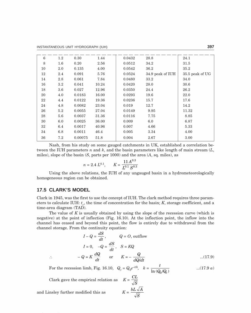
C-9\N-HYDRO\HYD17-1.PM5 397
INSTANTANEOUS UNIT HYDROGRAPH (IUH) 397
6 1.2 0.30 1.44 0.0432 28.8 24.18 1.6 0.20 2.56 0.0512 34.2 31.5
10 2.0 0.135 4.00 0.0542 36.2 35.212 2.4 0.091 5.76 0.0524 34.9 peak of IUH 35.5 peak of UG14 2.8 0.061 7.84 0.0480 33.2 34.016 3.2 0.041 10.24 0.0420 28.0 30.618 3.6 0.027 12.96 0.0350 24.4 26.220 4.0 0.0183 16.00 0.0293 19.6 22.022 4.4 0.0122 19.36 0.0236 15.7 17.624 4.8 0.0082 23.04 0.019 12.7 14.226 5.2 0.0055 27.04 0.0149 9.95 11.3228 5.6 0.0037 31.36 0.0116 7.75 8.8530 6.0 0.0025 36.00 0.009 6.0 6.8732 6.4 0.0017 40.96 0.007 4.66 5.3334 6.8 0.0011 46.4 0.005 3.34 4.00
36 7.2 0.00075 51.8 0.004 2.67 3.00
Nash, from his study on some gauged catchments in UK, established a correlation be-tween the IUH parameters n and k, and the basin parameters like length of main stream (L,miles), slope of the basin (S, parts per 1000) and the area (A, sq. miles), as
n = 2.4 L0.1, K = 11 0.3
0.1 0.3
AL S
Using the above relations, the IUH of any ungauged basin in a hydrometeorologicallyhomogeneous region can be obtained.
17.5 CLARK’S MODEL
Clark in 1945, was the first to use the concept of IUH. The clark method requires three param-eters to calculate IUH: tc, the time of concentration for the basin; K, storage coefficient, and atime-area diagram (TAD).
The value of K is usually obtained by using the slope of the recession curve (which isnegative) at the point of inflection (Fig. 16.10). At the inflection point, the inflow into thechannel has ceased and beyond this point, the flow is entirely due to withdrawal from thechannel storage. From the continuity equation:
I – Q = dSdt
, Q = O, outflow
I = 0, –Q = dSdt
, S = KQ
∴ – Q = K dQdt
or K = – Q
dQ dt/...(17.9)
For the recession limb, Fig. 16.10, Qt = Q0e–t/k, k =
tQ Qtln ( / )0
...(17.9 a)
Clark gave the empirical relation as K = CL
S
and Linsley further modified this as K = bL A
S

C-9\N-HYDRO\HYD17-1.PM5 398
398 HYDROLOGY
K in hr, L in miles, A in sq. miles, constants C = 0.8 to 2.2, b = 0.04 to 0.08. The value ofK may be estimated from the above relations in case no hydrograph is available for the basin.
17.6 DRAWING ISOCHRONES AND TIME-AREA DIAGRAM (TAD)
The basin is divided into zones (sub-areas Ar, km2) by drawing isochrones (Fig. 16.11). Anisochrone is a line joining all points having the same travel time. A water particle on a 8-hrisochrone will take 8 hr to reach the basin outlet.
For drawing the isochrones, the profile of the longest water course (i.e., main watercourse) is plotted as ‘‘elevation vs, distance’’ from the basin outlet. The total length of the mainchannel is then divided into N reaches, keeping in mind the slopes in different reaches, since
the time of travel (t) is proportional to L/ S , i.e., t = KL
S , where K is the constant of propor-
tionality. Then the elevation of each portion in transferred to the contour map of the catch-ment.
An initial estimate of the time of concentration (tc hr) may be obtained by using Kirpich’sformula (L in km)
tc = 0.06628 L0.77 S–0.385 ...(17.10)and from this the value of K can be determined.
At the points transferred to the contour map, curves are drawn joining all the pointshaving specified travel times, which are called isochrones. The areas between the successiveisochrones are planimetered and the time-area diagram (TAD) is prepared from the isochronalmap (Fig. 16.12).
17.7 CLARK’S METHOD
In the Clark’s approach, the ordinates of TAD are converted to volume rate of runoff in cumecfor unit rainfall excess, i.e., 1 cm, occurring instantaneously and uniformly over thecatchment, as
I = 1 10100 60 60
6cm ( )At
r ×× ×
= 2.78 Atr cumec or m3/s ...(17.11)
where t = Computation time interval, hr of TAD, i.e., isochrone interval or routing periodtc = t × N, N = No. of inter-isochrone areas or sub areas, Ar km2
Catchment are A = ΣAr
In Example 16.1, tc = 1 hr × 9 # = 9 hr ~− ti, N = 9Note: 8 Isochrones are drawn to yield 9 zones (N = 9) or Subareas Ar.
t = tNc ...(17.12)
The inflow (I) from the sub area Ar calculated as above, i.e., the resulting translationhydrograph is then routed through a linear reservoir to simulate the storage effects of thebasin; Clark’s method utilises Muskingum method of routing through a linear reservoir, i.e.,x = 0 in Eq. (9.9); S = KQ, Q = O.
The general equations for the linear reservoir is (See Eq. (16.21))IUHO = O2 = Q = C′I + C2O1, O1 = Q1
i.e., Q2 = C′I + C2Q1, for IUH derivation ...(17.13)

C-9\N-HYDRO\HYD17-1.PM5 399
INSTANTANEOUS UNIT HYDROGRAPH (IUH) 399
The routing coefficients are obtained from (see Eqs. 16.20, 16.20a, 16.21)
C′ = t
k t+ /2 , C2 =
k tk t
−+
//22
∴ C′ + C2 = 1 ...(17.14)
The resulting IUHO (IUH ordinates) are averaged at tr intervals to produce a tr-hr UG,Ex. 16.1.
Note: ut of tr-hr UG = ut
tr−FHG
IKJ2
of IUH = u ut t tr
+ −
2 of IUH, i.e., by averaging IUHO, assuming linear.
Example 17.3 The recession ordinates of the flood hydrograph (FHO) for the Lakhwar damsite across river Yamuna are given below. Determine the value of K.
Time (hr): 30 36 42 48 54 60 66 72 78FHO (cumec): 1070 680 390 240 150 90 45 30 20
Solution Eq. (5.1) can be expressed in an alternative form of the exponential decay as
Qt = Q0 e–t/k, when K =
tQ Qtln ( / )0
‘Q vs. t’ is plotted on the semi-log paper (Fig. 17.1). K is the slope of the recession-flood-hydrograph plot.
2000
500
11001000
800:8
6
500:5
4
300:3
200:2
150:1.5
100
8
6
5
4
3
2
1.5
100 10 20 30 40 50 60 70 80 90 100 120
10
Time t (hr)
Q(c
umec
)
31 hr31 hr
ÑÑtt
Semi-log paper
SlopeK = – = –D
Dt
ln Q31 – 59
ln 1000100
– 12 hr
100cumec
1000
One logcycle
One logcycle
Rec
essi
onhy
drog
raph
Ord
inat
es(F
HO
)
59 hr59 hr
28
2.303 × log 10=
~
Fig. 17.1 Recession flood hydrograph

C-9\N-HYDRO\HYD17-1.PM5 400
400 HYDROLOGY
K = ∆
∆∆t
Qt
ln . log=
2 3031000100
, ∆t = t1000 – t100 cumec
= 31 hr – 59 hr, from the plot
K = 31 59
2 303 128
2 30312 15
−×
= − = −. .
. , say 12 hr
Example 17.4 The isochronal map of Lakhwar damsite catchment, Fig. 17.2 (a) has areasbetween successive 3 hr isochrones as 32, 67, 90, 116, 135, 237, 586 and 687 km2. Taking k = 12hr (as determined in Ex. 17.3), derive the IUH of the basin by Clark’s approach and hence a3-hr UG.
0 3 6 9 12 15 18 21 24
Time (hr)
(b) Time-area diagram (TAD)
A1A2
A3A4
A5
A6
A7
A8
t = t= 3 hr
cÑ
t 8 = 24# hrA ll
t
c
r
c
´
700
600
500
400
300
200
100
Inte
r-is
ochr
one
area
A(k
mr
2 )
Remoteend
t = 24 hrc21 hr
7
21hrHanuman
A Ganga8
R.YamunaR.Yamuna
A 7
Bhadri GadBhadri Gad
A4
A5
A6A3
A2
A1
Basinboundary
6
5
12 hr-49 hr-36 hr-23 hr-1LakhwarD.S.
R.Yamuna
Basin outletMussorie
9hr
12hr
15hr
18hr
(a) Isochronal map of LakhwarDS Catchment.
3 hr-Isochrones, 7 #subareas: A -A1 8
A = A = 1950 km
t = 24 hr, t = t = 3 hr
S r
c c
2
Ñ
8
1
3 hr 8 # = 24 hr= t
´c
Fig. 17.2 Isochrones and TAD for Lakhwar Dam Site
SolutionNote A = ΣAr = 1950 km2
tc = t × N = 3 × 8 = 24 hr, K = 12 hr No. of isochrones = N – 1 = 8 – 1 = 7#
Computation interval t = ∆tc between successive isochrones = 3 hr = 248
=tc
N
Clark’s approach Eq. (17.13): Q2 = C′I + C2Q1
C′ = t
k t+ /2 = 3
1232
+ = 0.2222, C2 =
k tk t
−+
= −+
//
//
22
12 3 212 3 2
= 0.7778
Check: C′ + C2 = 0.2222 + 0.7778 = 1 ∴ O.K.

C-9\N-HYDRO\HYD17-1.PM5 401
INSTANTANEOUS UNIT HYDROGRAPH (IUH) 401
From the sub areas Ar, Eq. (17.11): I = 2.78 Atr = 2.78 ×
Ar
3 = 0.9267 Ar
Clark’s: Q2 = C′I + C2Q1, C2Q1 = 0.7778 Q1 Q2 = IUHOC′I = 0.2222 × 0.9267 Ar = 0.203 Ar
Table 17.3 Computation of IUH by Clark’s approach and hence 3-hr UG.
1 2 3 4 5 6
Time Ar , (km2) C′I C2Q1 IUHO 3-hr(hr) (from = 0.203 Ar = 0.7778 Q1 Q2(cumec) UGO
TAD) = (2) × 0.203 = (5) ×0.7778 = C′I + C2Q1 (cumec)previous = (3) + (4) (by averaging)
0 0 0 0 0
3 32 6.4 + 0 6.40 6 4
2+ .
= 3.2
6 67 13.5 + 5.1 18.66 4 18 6
2. .+
= 12.5
9 90 18.0 + 14.9 33.0 25.3
12 116 23.3 26.4 49.7 41.3
15 135 27.0 39.7 66.7 58.2
18 237 47.5 53.0 100.5 83.6
21 586 117 80.0 197.0 148.8
24 687 137.5 157 294.5 245.7
27 ΣAr = 1950 km2 0 230 230 262.2
30 0 179 179 204.5
33 0 139.5 139.5 159.2
Plot Col. (5) vs. col (1) to get IUH, and Col (6) vs. col. (1) to get 3-hr UG. Note that the two peaksare staggered by 3 hr; i.e., IUH is more skewed.
�������
1 Define IUH and state its important properties illustrated in a neat sketch. What are the advan-tages of IUH over a UG of finite duration?
2 Determine the values of n and k, and hence derive an IUH for the drainage basin in Example 5.2.State its peak and time to peak.
3 For the IUH obtained in (2) above, derive a 6-hr UG and compare with that obtained inExample 5.2.
4 Derive an IUH by Clark’s approach and hence a 2-hr UG for a catchment of 140 km2, tc = 18 hr,K = 12 hr. The catchment was divided into 9 zones by drawing 8 isochrones. The areas planimeteredbetween the successive 2-hr isochrones are 8 (near outlet) 12, 25, 35, 22, 16, 10, 8 and 4 (remoteend) in km2.
peak ofIUH
× 0.78
× 0 .78
(peakof UG)

C-9\N-HYDRO\HYD17-1.PM5 402
402 HYDROLOGY
5 (a) Explain the concept of Clark’s IUH.
(b) The shape of a catchment can be approximated to a square with diagonal of 60 km. The mainchannel is nearly along a diagonal; the isochrones may be assumed perpendicular to themain channel. The travel speed along the main channel may be taken as 5 km/hr. Derive theIUH for the basin with K = 5 hr
Hint: tc = 12 hr. Divide the diagonal into 6 parts to obtain successive 2-hr isochrones.
6 The IUH of a basin can be approximated to a triangle of base 36 hr and peak of 30 cumec at 9 hrfrom the start. Derive a 3-hr UG for this basin.

Chapter 18
403
CLOUD SEEDING
18.1 CONDITIONS FOR CLOUD SEEDING
Between the vanishing forests and the reluctant clouds, the draught has advanced menac-ingly. This is where cloud seeding will help win the battle.
Cloud seeding was discovered as accidentally as most scientific discoveries. In 1946,when Dr. Vincent J. Schaefer working with GE in New York was trying to create artificialclouds in a chilled chamber, he placed dry ice inside to cool the chamber. Water vapour insideformed a cloud around the dry ice. That is pretty much how in a normal cloud ice crystals formwhen cold water contacts particles of dust, salt or soot.
In clould seeding, silver iodide or other agents like common salt are introduced, whichmimic the ise crystal; the number of these nuclei available is increased and these can take inmore moisture in the cloud and form raindrops, which otherwise would not have formed. Thisincreased condensation and freezing releases a large amount of heat that makes clouds morebuoyant and extends them sidewards and upwards. As clouds grow taller, their updraft in-creases, they draw in more moist air from the near surface and their size increases further.
Enlarged clouds then encroach over several smaller clouds nearby and grow further,and hence the duration and quantity of rainfall will increase.
Rain clouds 6–9 km high and containing 0.5 mcm (million cubic meter) of water seededwith silver iodide can be raised by 2 km and their water content increased to >1 mcm. Seedingof multi-cell clouds leads to very high precipitation as compared to single cell clouds. Cloudseeding has been carried out quite successfully in several countries including USA, Israel,Russia, Canada, Australia and India. Clouds have been seeded at a height of around 2 kmabove sea level.
However, it should be known that cloud seeding can only accelerate and increase theamount of rainfall and not create rainfall, when the conditions are not favourable, as what hap-pened when seeding was done in 1975 in Linganamakki area of Sagar (Shimoga Dist., Karnataka);the seeded clouds had drifted away do to wind; also the clouds were floating below 1.2 km level.
Cloud seeding can not be done in the areas where there are no chouds as it can onlymake the bad clouds to yield more.
The conditions favourable for cloud seeding are:(i) the lower surface of the clouds should be within 1 km from the ground surface.

C-9\N-HYDRO\HYD18-1.PM5 404
404 HYDROLOGY
(ii) the relative humidity must be high, >75% and wind velocity < 15–20 km/hr.(iii) the temperature inside the cloud should be less than the freezing point of water.Cloud seeding can be done either from above or from below, as illustrated in the following.Seeding from above is resorted when a large area is concerned. This requires special
aircraft that can travel to heights where precipitation occurs, and can carry large loads ofseeding material. The four major requirements are:
(i) equipment of clould-condensation-nuclei measurement,(ii) facility for photographing of cloud growth,
(iii) temperature measurement, and(iv) 2-D Doppler Echo measurement of precipitation particles.The weather radars are setup at land surface at air bases for locating the movements of
rain potential clouds and will cover nearly 400 km2. A Doppler weather radar with a range of200–400 km was setup at air bases of Bidar, Hubli and Jakkur (in Karnataka).
The operation of monitoring the rain efficient clouds are done through the computer-aided system on board the cloud seeding aircraft with the support of the communication devicesfrom the base station. The turbo-prop aircraft titled Piper-PA 31 with special equipment andextra fittings arrived from the US-based Weather Modifications Inc. (WMI) for enhancing therainfall by 25% in the drought-hit districts of Karnataka following the failure of rainfall for thethird consecutive year at a cost of Rs. 5.6 crore, in August 2003. The tender proposal wasprepared by experts from IITM and IMD.
The WMI, a cloud seeding company based in Fargo, north Dakota in the USA, has carriedout cloud seeding operations in fifteen countries and most of their operations were successful.WMI had quoted Rs. 8 crore for the cloud seeding operations in Karnataka in August 2003.WMI’s competitor was Atmospheric INC. (AI), which is also a US-based company.
Experts of WMI started the 90-day ‘‘Project Varuna’’ from August 18, 2003. The WMIhad the radar and control room at Agni Aerosports in Jakkur Airfield at Bangalore. The radarto scan for rain-bearing clouds in the range of 200 km and give informulation to the pilot andcrew of the aircraft, who in turn fly to the region and carry out the cloud seeding operations.
While the popular form of cloud seeding is through spraying from aircraft, approachfrom below also has been used, as in Hyderabad in July 1993. Using ground generatorsconsisting of hot ovens and a blower, coal is heated to 1200 °C and silver iodide sprinkled. Therising fumes went straight into the sagging clouds. In minutes-there was a downpour for halfan hour resulting in increased waterlevel in Osman Sagar Lake (Hyderabad). The samplesshowed traces of silver iodide proving the rains were due to the seeding.
18.2 CLOUD SEEDING TECHNIQUE
When nature is reluctant to produce ice in super-cooled clouds, it is possible to lend a hand byproviding the ice nuclei that nature is lacking. This is commonly called cloud seeding and itcould be done with a variety of ice-inducing agents like silver iodide or sodium chloride.
When silver iodide is used, small amounts are burned in flares or solution at the cloudtop or in the updrafts at the cloud base with the help of aircraft flying, the rapid developmentof large number of small ice droplets soon follows.
When sodium chloride is sprayed on to the clouds with the help of aircraft, it precipi-tates the cloud particles, which are usually of 100 microns, µ, (1000 µ = 1 mm), into larger

C-9\N-HYDRO\HYD18-1.PM5 405
CLOUD SEEDING 405
particles upto 6-7 mm. When the particles increase in size, they can not hold together andcome down to the earth resulting in rain. This precipitation also happens naturally duringnormal rains.
Fig. 18.1 A hygroscopic cartridge being burnt to demonstrate the processof cloud seeding, which was inaugurated at the Jakkur airfield in Bangalore on Monday-Aug. 2003
Fig. 18.2 An aircraft fitted with flares containing nuclei used for cloudseeding operation can be seen in this file photo

C-9\N-HYDRO\HYD18-1.PM5 406
406 HYDROLOGY
Cloud seeding however, artificially presses the cloud particles to precipitate and resultin rain. The chances of rains increase by about 30% due to cloud seeding.
Though sodium chloride is normally used in the tropical region which gets Warm rains(where small cloud particles become bigger resulting in rain), silver iodide is used in coldrains (which occur in high altitudes) in which water particles in cloud freeze and in turnresult in rain. Silver iodide enhances the chances of water particles freezing.
Both the chemicals were used for cloud seeding in Karnataka during August 2003.
18.3 CLOUD SEEDING OPERATION
To begin with, one has to identify the clouds, which can not yield rains due to shortage of (ice/water) nuclei; after that, the exact number of nuclei to be added to such clouds to make themyield rains, has to be found out.
Then, the technical team will calculate the quantity of silver iodide that has to be addedto the clouds to get the required increase in nuclei. This could be done through computer-aidedsystem on board the aircraft with the input as well as communication from the base-station.The addition of nuclei would be facilitated by burning silver iodide flares. The crew may haveof six members—two pilots, two meteorologists and two technicians for carrying out the cloudseeding operations. The aircraft should be capable of 6 hr endurance at operational altitudes,having computer-aided control for scientific management of cloud sceding operations.
Cloud seeding is not so costly and the benefit-cost ratio may be around 60: 1. Severalscientists are still sceptical as to how effective the cloud seeding is ! Is the rain in most casesdue to the seeding or was it anyway poised to rain, they ask. But one thing they all agree, isthat there have been no negative effects from cloud seeding so far with regard to polluting theenvironment or the chemicals used. The criticisms are about the possibility of creating badweather or floods; and of course increasing rainfall in one region is at the expense of rainfall ina neighbouring local region.
18.4 RECENT CASE HISTORY
Russian air force’s special squad air craft was pressed into service on Monday (9th May 2005)to clear cloud-cover over MOSCOW, so that no rain clouds dampen the Victory Day celebrations(marking the 60th anniversary of the Allied Victory over Nazi Germany in World War II)attended by leaders of 53 nations.
At 5.30 A.M. (local time), 12 Antonov An-12 and Ilyushin IL-18 aircraft took position inthe sky over Moscow, divided in 10 zones, as a cyclone from the west advanced towards thecapital.
Flying at 3-8 km altitude, the planes sprinkled various chemicals including silver iodide,liquid nitrogen, dry ice (frozen carbon dioxide) and even ordinary cement to seed the clouds ata distance of 50-150 km away. By 10 A.M. sharp at the start of the military parade, rain hadstopped in Red Square and the sky was clear for the impressive flypast by Sukhoi and MIGfighters. For the first time in Moscow, computer-designed fireworks were used on Mondaynight, and the efforts were to keep the sky clear till date in the night.

In most parts of the Western Countries, snowmelt produces the major portion of theannual runoff. The high altitudes in the Himalayan range are snow covered and there is anappreciable snowmelt runoff in the rivers, which originate from the Himalayan range.
Snow cover is usually more variable than precipitation within a given area. Thehydrologist is concerned with the structure attained by the snow just prior to melting, the areaand depth of snow pack, the rates of snowmelt, and the resulting runoff in the stream due tosnowmelt and concurrent rainfall. The measurements of snow depths can be done by snowsurvey, snow gauging, and remote sensing by satellite.
Physics of SnowmeltThe sources of energy to melt snow may be broadly classified as:
(i) radient heat from the sun,
(ii) latent heat of vapourisation released by condensation of water vapour, and
(iii) heat by conduction from the environment of snow, such as from the ground, rainfall,and air.
The snow pack may also loose heat to its environment by radiation, sublimation and byconductivity. The melting of snow, due to the interactions of the various phenomena of heatexchange, makes it one of the most complex in the field of hydrology.
The most common source is solar radiation. The amount of radiation effective in themelting of snow is dependent on its reflectivity or albedo. About 90 per cent of the radiationincident on clean, fresh snow is reflected (without causing melt), while lesser amounts arereflected from old and dirty snow.
Conduction from still air causes very little melt (due to its low heat conductivity). Tur-bulence resulting from wind, brings large quantities of warm air into contact with the snow,and heat exchange takes place. If the dew point of the air is less than the snow-surface tem-perature, the vapour pressure of snow (es) is greater than that of the air (ea) resulting in evapo-ration from the snow surface; on the other hand, if the dew point is above freezing, condensa-tion on the snow occurs, with consequent release of latent heat.
Appendix A
SNOWMELT RUNOFF
407

C-9\N-HYDRO\APP.PM5 408
408 HYDROLOGY
Snow melt (Ms) due to convection is proportional to the difference in temperature of theair (Ta) and the snow (Ts), while due to conduction the snowmelt is proportional to the vapourpressure gradient (ea – es) ; both the two processes are influenced by the wind speed (Vw) andare given by
Ms (air-convection) = kc(Ta – Ts)Vw
Ms (vapour-condensation) = kv(ea – es)Vw
where Ts = 0 °C es = saturation vapour pressure in mb at 0 °C (= 6.11)
kc, ky = exchange coefficients Vw = average wind speed
If the vapour pressure of the air is higher than that of ice at 0 °C, the moisture (vapour)brought by turbulence in the air, condences on the snow surface. Since the condensation ofwater at 0 °C is 596 cal/g and the heat of fusion of ice is 80 cal/g, the condensation of 10 mm of
water vapour on the snow surface causes 59680
× 10 = 7.5 × 10 = 75 mm of melt water from the
snow. Hence, the wind speed (which causes turbulence) is an important factor in computingsnowmelt.
Rainfall, at temperature above freezing, causes snowmelt and is given by the simplecalorimetric equation
Ms = PTw
80where Ms = snowmelt (mm)
P = rainfall (mm)Tw = wet-bulb temperature (°C)
If Tw = 20 °C, 20 mm of rain will cause 20 20
80×
= 5 mm of melt water from the snow.
Thus rainfall is less effective in causing snow melt, while the strong winds, warm air and highhumidity which accompany rainfall cause appreciable melt during rainstorms.
Forest cover, land slope (topography), influence wind, temperature and humidity of theair, and appreciably affect the amount of radiation incident on snow; hence, the importance ofenvironment on the snowmelt.
If the basin is covered with a fairly uniform depth of snow, the snowmelt can be esti-mated by the use of the ‘degree-day factors’. The degree-day factor is the depth of water meltedfrom the snow in mm per degree-day, i.e., mean daily temperature of 1 °C above freezingtemperature (0 °C), and can be determined by dividing the volume of streamflow as a result ofsnowmelt during a certain period by the total degree-days for the period. The factor usuallyranges form 2-7 mm/degree-day. Since solar radiation, humidity and wind affect snowmelt,some variation in the degree-day factor from day to day may be expected and seems to increaseas the melting period progresses*, Fig. A-1. There is a time lag between the snowmelt and thestreamflow observed, so that the latter is not a measure of the former.
*Linsley R. K., A Simple Procedure for Day-to-Day Forecasts of Runoff from Snow Melt, Trans.Am. Geophys. Union, Vol. 24, pp. 62-67, 1943.
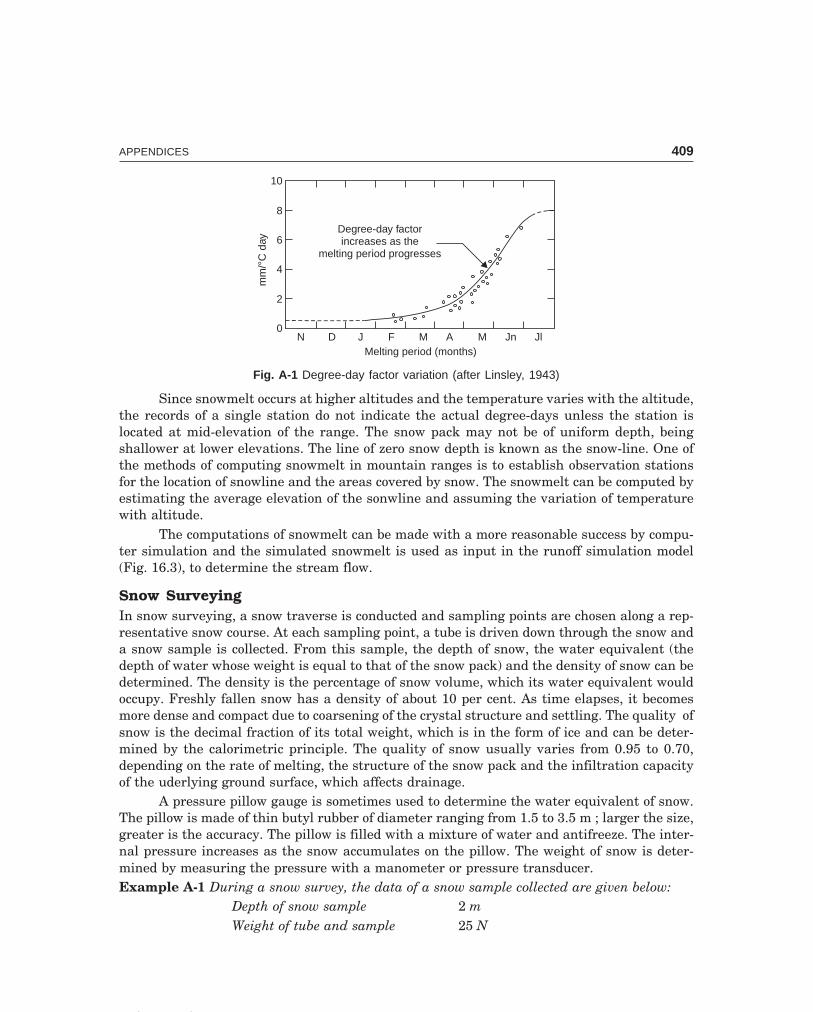
C-9\N-HYDRO\APP.PM5 409
APPENDICES 409
Degree-day factorincreases as the
melting period progresses
N D J F M A M Jn JlMelting period (months)
10
8
6
4
2
0
mm
/°C
day
Fig. A-1 Degree-day factor variation (after Linsley, 1943)
Since snowmelt occurs at higher altitudes and the temperature varies with the altitude,the records of a single station do not indicate the actual degree-days unless the station islocated at mid-elevation of the range. The snow pack may not be of uniform depth, beingshallower at lower elevations. The line of zero snow depth is known as the snow-line. One ofthe methods of computing snowmelt in mountain ranges is to establish observation stationsfor the location of snowline and the areas covered by snow. The snowmelt can be computed byestimating the average elevation of the sonwline and assuming the variation of temperaturewith altitude.
The computations of snowmelt can be made with a more reasonable success by compu-ter simulation and the simulated snowmelt is used as input in the runoff simulation model(Fig. 16.3), to determine the stream flow.
Snow SurveyingIn snow surveying, a snow traverse is conducted and sampling points are chosen along a rep-resentative snow course. At each sampling point, a tube is driven down through the snow anda snow sample is collected. From this sample, the depth of snow, the water equivalent (thedepth of water whose weight is equal to that of the snow pack) and the density of snow can bedetermined. The density is the percentage of snow volume, which its water equivalent wouldoccupy. Freshly fallen snow has a density of about 10 per cent. As time elapses, it becomesmore dense and compact due to coarsening of the crystal structure and settling. The quality ofsnow is the decimal fraction of its total weight, which is in the form of ice and can be deter-mined by the calorimetric principle. The quality of snow usually varies from 0.95 to 0.70,depending on the rate of melting, the structure of the snow pack and the infiltration capacityof the uderlying ground surface, which affects drainage.
A pressure pillow gauge is sometimes used to determine the water equivalent of snow.The pillow is made of thin butyl rubber of diameter ranging from 1.5 to 3.5 m ; larger the size,greater is the accuracy. The pillow is filled with a mixture of water and antifreeze. The inter-nal pressure increases as the snow accumulates on the pillow. The weight of snow is deter-mined by measuring the pressure with a manometer or pressure transducer.Example A-1 During a snow survey, the data of a snow sample collected are given below:
Depth of snow sample 2 mWeight of tube and sample 25 N

C-9\N-HYDRO\APP.PM5 410
410 HYDROLOGY
Weight of sample tube 20 NDiameter of tube 40 mm
Determine(i) the density of snow
(ii) the water equivalent of snow(iii) the quality of snow, if the final temperature is 5 °C when 4 lit. of water at 15 °C is
added.Solution (i) Density of snow is the same as its specific gravity
Sp. gr. of snow, Gs = γγ γ
s
w
s s
w
W V=
/ =
( ) / ( . ).
25 20 0 020 21000 9 81
2− ××
π = 0.203
(ii) Density of snow, Gs = Depth of melt water
Depth of snow( )
( )d
dw
s
∴ Water equivalent of snow, dw = Gsds = 0.203 × 2 = 0.406 m(iii) If the actual weight of ice content in the sample is Wc gm, thenHeat gained by snow = Heat lost by waterHeat required to melt + to rise temperature to 5 °C
Wc × 80 + 5
9 81. × 1000 × 5 = 4000(15 – 5)
Solving, Wc = 468.2 gm = 0.4682 × 9.81 = 4.6 N
∴ Quality of snow = 4 65.
= 0.92
Example A-2 If the density of a snow pack 1.2 m depth is 20%, determine its weight density,mass density, sp. gr. and water equivalent.Solution The density is the percentage of snow volume, which its water equivalent wouldoccupy.
∴ Snow density = Depth of melt water
Depth of snow( )
( )d
dw
s
∴ 0.20 = dd
w
s
Water equivalent of snow, dw = 0.20 × 1.2 = 0.24 m
Weight density, γs = WV
WV
VV
dd
s
s
w
s
w w
s
w
s= = =
γ γw
= 0.20 (1000 × 9.81) = 1962 N/m3
Mass density, ρs = MV
W gV g
s
s
s
s
s= = =/
.γ 1962
9 81 = 200 kg/m3
Sp. gr., Gs = γγ
s
w=
×1962
1000 9 81. = 0.2
Note, that the specific gravity is the same as the snow density.
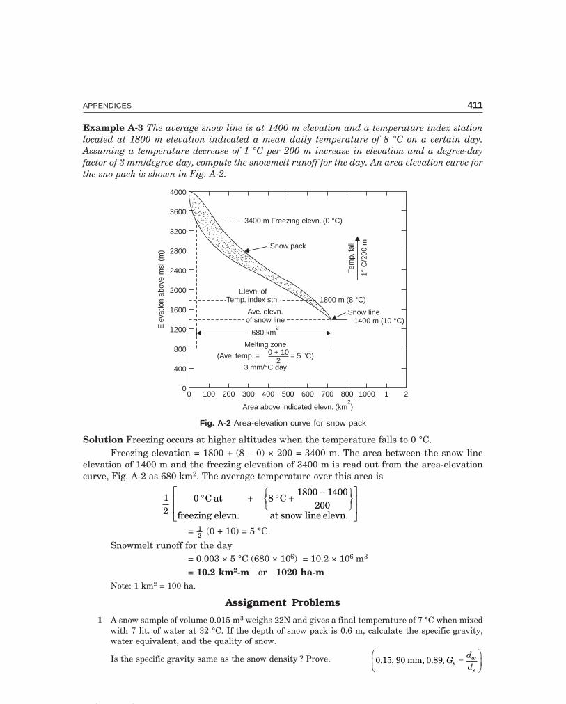
C-9\N-HYDRO\APP.PM5 411
APPENDICES 411
Example A-3 The average snow line is at 1400 m elevation and a temperature index stationlocated at 1800 m elevation indicated a mean daily temperature of 8 °C on a certain day.Assuming a temperature decrease of 1 °C per 200 m increase in elevation and a degree-dayfactor of 3 mm/degree-day, compute the snowmelt runoff for the day. An area elevation curve forthe sno pack is shown in Fig. A-2.
4000
3600
3200
2800
2400
2000
1600
1200
800
400
00 100 200 300 400 500 600 700 800 1000 1 2
Area above indicated elevn. (km )2
Ele
vatio
nab
ove
msl
(m)
3400 m Freezing elevn. (0 °C)
Snow pack
Tem
p.fa
ll
1°C
/200
m
1800 m (8 °C)
Snow line1400 m (10 °C)
Elevn. ofTemp. index stn.
Elevn. ofTemp. index stn.
Ave. elevn.of snow lineAve. elevn.of snow line
680 km2
680 km2
Melting zone
(Ave. temp. = 5 °C)
3 mm/°C day
=0 + 102
Fig. A-2 Area-elevation curve for snow pack
Solution Freezing occurs at higher altitudes when the temperature falls to 0 °C.Freezing elevation = 1800 + (8 – 0) × 200 = 3400 m. The area between the snow line
elevation of 1400 m and the freezing elevation of 3400 m is read out from the area-elevationcurve, Fig. A-2 as 680 km2. The average temperature over this area is
12
0 8
1800 1400200
° + ° +−RST
UVWL
NMM
O
QPP
C at C
freezing elevn. at snow line elevn.
= 12 (0 + 10) = 5 °C.
Snowmelt runoff for the day= 0.003 × 5 °C (680 × 106) = 10.2 × 10⁶ m3
= 10.2 km2-m or 1020 ha-mNote: 1 km2 = 100 ha.
Assignment Problems
1 A snow sample of volume 0.015 m3 weighs 22N and gives a final temperature of 7 °C when mixedwith 7 lit. of water at 32 °C. If the depth of snow pack is 0.6 m, calculate the specific gravity,water equivalent, and the quality of snow.
Is the specific gravity same as the snow density ? Prove. 0.15, 90 mm, 0.89, Gddsw
s=
FHG
IKJ

C-9\N-HYDRO\APP.PM5 412
412 HYDROLOGY
2 For a certain period in a mountain range, the degree-day factor is 4 mm/°C-day. How much thedepth of snow pack decreases on a warm spring day with maximum and minimum temperaturerecorded as 25 °C and 7 °C, respectively. Assume a sp. gr. of 0.16 for the snow. If the area coveredby snow is 450 km2, estimate the snowmelt runoff on the day.
Whether this snowmelt and the stream flow observed on the day are concurrent? Explain.(0.4 m, 28.8 Mm3)

In open-channel hydraulics, overland flow is considered as sheet flow, a spatially variedunsteady flow. Many investigators have made analysis of overland flow and Izzard’s methodhas been found to be more practical.
Laminar Overland FlowFor small plots without defined channels, with short, mild, uniform slopes, such as parkinglots, airports, runoff occurs as laminar overland flow for which the critical Reynolds number isgiven by
Re = Vd qν ν
= < 1000 ...(1)
where d and q are the uniform depth and discharge per meter with of overland flow, respec-tively. Izzard has suggested that for rectangular plots, laminar flow occurs if
inet l < 4000 ...(2)where inet is the net rainfall in mm/hr, and l, b are the length and breadth of the plot in metres.Since q = inet l, Eqs. (1) and (2) in consistent units agree.
Forces under steady, uniform laminar overland flow are shown in Fig. B-1; forces on theelement of water P1 = P2. For steady flow and for b = 1
τ(∆x . 1) = ∆W sin αPutting sin α = tan α = S
for small values of α, S is the land slope, τ is the shear stress at a depth y above the landsurface. Substituting for ∆W,
τ ∆x = ∆ x (d – y) γw Sor τ = γw S(d – y)
Putting y = 0, the bed shear τ0 = γw dS ...(3)From the Newton’s law of viscosity,
τ = µ dvdy
Appendix B
OVERLAND FLOW
413

C-9\N-HYDRO\APP.PM5 414
414 HYDROLOGY
P
Water sheet
t g0 w= d S
a
t0t0
Sa
Land slope
W
W sin a sin a = tan = Sa
(a) Forces acting on water sheet
t
Sa
Land slope, S
DW = x 1(d – y)D gw
Pd
Pdd
Element of water
a
v
vs
P
Dx x1Dx x1
DW sin a(b) Forces acting on the water element
y
V
Fig. B-1 Overland flow analysis
µ dvdy
= γwS(d – y)
dv = γ
µwS
(d – y)dy
Integrating both sides,
z dv = γ
µwS
d y dyz −( )
v = γ
µwS
dyy−
FHG
IKJ
2
2 + C
At the land surface, y = 0, v = 0, ∴ C = 0.The velocity at any depth y above the land surface is given by the parabolic equation
v = γ
µwS
dyy
−FHG
IKJ
2
2...(4)
Mean velocity V is given by
V = 1
0dvdy
dz = 1
20
2
dS
dyyd
wz −FHG
IKJ
γµ
dy, from Eq. (4)
∴ V = γ
µwS3
d2 ...(5)

C-9\N-HYDRO\APP.PM5 415
APPENDICES 415
The discharge, q = Vd,
q = γ
µwS3
d3 ...(6)
Note that q ~ d3S, so that if q is constant but slope S varies, d and V at another sectioncan be estimated.
The velocity at the water surface vs is obtained by putting y = d in Eq. (4)
vs = γ
µwS2
d2 ...(7)
which is the maximum velocity.
0
Shear-
stress
distributionvs
vv
VV
x
Parabolic
vel. distribn.Parabolic
vel. distribn.
yy
d-yd-y
ddSheet
of water
S
0.58d0.58d
Fig. B-2 Laminar overland flow
From Fig. B-2, v = vs – x
vvs
= 1 – xvs
x = vs – v
x = γ
µwS2 [d2 – (2dy – y2)] from Eqs. (4) and (7)
xvs
= d dy y
d
d y
d
2 2
2
2
22− +
=−( )
∴ vvs
= 1 – d y
d−F
HGIKJ
2
...(8)
when v = V, Vvs
= 1 – d y
d−F
HGIKJ
2
Since the velocity distribution is parabolic, the mean velocity V is two-thirds of the
maximum velocity vs, i.e., V = 23
vs, orVvs
= 23
23
= 1 – d y
d−F
HGIKJ
2
ord y
d−F
HGIKJ
2
= 13

C-9\N-HYDRO\APP.PM5 416
416 HYDROLOGY
∴ d – y = 0.58 d ...(9)which is in close agreement with the mean velocity position for turbulent stream flow (≈ 0.6 dor mean of the velocities at 0.2 d and 0.8 d).
Turbulent Overland FlowThe equation for the turbulent over land flow can be obtained by using the Manning’s equation
q = (d . 1)V = (d . 1) 1n
R2/3 S1/2
Since the hydraulic mean radiusR ≈ d, for broad surfaces
q = 1n
d5/3 S1/2 ...(10)
From Eqs. (6) and (10), for both laminar and turbulent overland flows, from theory andexperiments, the equation of flow is of the general form
qe = KdemSn ...(11)
Where K, m and n are constants varying with the Reynolds number Re, raindrop impact,and land roughness. For turbulent flow m = 1.67, n = 0.5 and for laminar flow, m = 3, n = 1. C.F.Izzard (1946) developed the expression for the laminar overland flow as
qe = Kde3S ...(12)
where K = 1
2 8 10 5
3
. × +
LNM
OQP− i C
qe = equilibrium flow in m3/S per m width of strip at the lower edge of the rectangulararea of uniform slope S.
de = volume of detention storage, expressed as the average depth over the full length ofthe strip of unit width, whereas in Eqs. (1) to (10), d is the depth at a particular section wherethe discharge is q.
i = the actual rainfall intensity in mm/hr, not the net rate, since the term 2.8 × 10⁻⁵ iis intended to represent the retarding effect of rain-drop impact.
C = a roughness factor depending upon the type of land surface. Experimental values ofC reported by Izzard are given below:
Type of surface Value of CConcrete pavement 0.012
Tar and gravel pavement 0.017
Tar and sand pavement 0.0075
Smooth asphalt pavement 0.007
Crushed-slate roofing paper 0.0082
Dense bluegrass turf 0.060
Closely clipped sold 0.046
Determination of Overland Flow Hydrograph from Rainfall DataEqs. (11) and (12) are for equilibrium flow conditions and will not give correct values for dis-charge during periods of unsteady flow, which occur during actual storms. Due to time lag

C-9\N-HYDRO\APP.PM5 417
APPENDICES 417
between rainfall and discharge, they give too high values of discharge during the rising stageand too low values during recession time. A simple method is to divide the net-rain hydrographto a few broad steps, as shown in Fig. B-3 and then draw the discharge hydrograph for eachstep. The rising hydrograph for the first step is obtained from the empirically deriveddimensionless S-hydrograph (Fig. B-4). The equilibrium time te is taken as the time when thedischarge q reaches 97 per cent of the equilibrium discharge qe and this provides a good keypoint.
1
2
3Net-rain
Time t (min)
Inte
nsity
i(m
m/h
r)
a. Hyetograph dividedinto steps 1, 2, & 3
b. Runoff hydrographfor each step
Run
off(
mm
/hr)
qe1
qe2
qe3
Overland flowhydrograph
Time t (min)
Fig. B-3 Overland flow hydrograph derived from rainfall data
b
a
a. rising limb b. recession curve1.0
0.9
0.8
0.7
0.6
0.5
0.4
0.3
0.2
0.1
00 0.1 .2 .3 .4 .5 .6 .7 .8 .9 1.0 .5 1 1.5 2 2.5 3 3.5 4 4.5 5
(t/t )e b-values
(q/q
e)
Fig. B-4 Izzard’s dimensionless graph (after Izzard, 1946)
Since the S-hydrograph divides the graphical plot approximately into two equal parts,the average discharge during the time te can be taken as qe/2, which should be equal to thevolume divided by the time, i.e.,
q d lt
e e
e2= ...(13)
from which the equilibrium time te can be computed.Izzard provides techniques for computing the transition hydrographs for higher steps
(when water is deeper and faster), shorter steps (when q does not reach qe) and the recessionperiods, based on Eq. (12).
The dimensionless recession curve Fig. B-4 defines the shape of the receding limb. Atany time ta after the end of rain, the factor β is given by
C-9\N-HYDRO\APP.PM5 418
418 HYDROLOGY
β = q td l
e a
e0...(14)
where in consistent units and deo = de taking i = 0.
Example B-1 Equilibrium overland flow occurs over a rectangular area 100 m long due to auniform net rainfall of 50 mm/hr. At what distance from the upper edge of the area the flowchanges from laminar to turbulent if the temperature is 20 °C and the critical Reynolds numberis 800.
Solution Re = vd qν ν
=
νwater at 20 °C = 0.01 St = 0.01 × 10⁻⁴ m2/S or 1 × 10⁻⁶ m2/S
800 = q
1 10 6× − ∴ q = 8 × 10⁻⁴ cumec/m
q = inet l, 8 × 10–4 = 50
1000 60 60× × × l
∴ l = 57.6 m, beyond which the flow becomes turbulent.Note: For laminar flow, inet l < 4000 (Izzard)
∴ l < 400050
, i.e., l < 80 m (this assumes critical Re = 1000)
Example B-2 A concrete-paved area is 200 m long by 100 m wide and has surface slope of0.005. The design storm is given by
i = 2500.4
(i–mm/hr, t-min)
Construct the outflow hydrograph for a 1-hr storm using Izzard’s method.
Solution Equilibrium discharge, qe = inet (l × 1); for t = 60 min, i = 250
600.4 = 48.5 mm/hr
Assuming i = inet for the concrete pavement (initially wet),
qe = 48 5
1000 60 60.
× × (200 × 1) = 0.0027 cumec/m
From Eq. (11), qe = Kde3S
Depth of flow de = qKS
eLNM
OQP
1/3
K1/3 = 1
2 8 10 5( . )× +− i C =
1
2 8 10 48 5 0 0125( . )( . ) .× +− = 1
0 01336.
� de = 0.01336 0 00270 005
1/3..
FHG
IKJ = 0.0131 m, or 13.1 mm
From Eq. (12), the equilibrium time
te = 2 2 0 0131 200
0 0027d lq
e
e=
× ×..
= 1940 sec = 32 min 20 sec

C-9\N-HYDRO\APP.PM5 419
APPENDICES 419D
ata
to p
lot
the
risi
ng
tim
bD
ata
to p
lot
the
rece
ssio
n c
urv
e
q/q e
Q ×
qeb
(×
0.2
7) =
(m
3 /s)
t/t e
t ×
t e (×
32.
33)
= (
min
)t a
(min
)β
= 0
069
ta
q/q e
(fro
m g
raph
)(×
0.2
7) =
Q (
m3 /
S)
00
00
50.
345
0.45
0.12
1
0.2
0.05
40.
3110
.07.
50.
517
0.30
0.08
1
100.
690
0.27
0.07
30.
40.
108
0.42
13.6
151.
035
0.18
0.04
9
201.
380.
130.
035
0.6
0.16
20.
5216
.825
1.72
0.11
0.03
0
302.
070.
090.
0243
0.8
0.21
60.
6721
.740
2.76
0.06
0.01
62
503.
450.
040.
0108
0.97
0.26
11.
0032
.360
4.14
0.03
50.
0094
654.
500.
030.
0081
Tab
le B
-1 T
o pl
ot t
he
outf
low
hyd
rogr
aph
usi
ng
Izza
rd’s
dim
ensi
onle
ss g
raph

C-9\N-HYDRO\APP.PM5 420
420 HYDROLOGY
0.30
0.25
0.20
0.15
0.10
0.05
00 5 10 15 20 25 30 35 40 45 50 55 60 5 10 15 20 30 40 50 60
After rain starts, t (min) After end of rain, t (min)a
Dis
char
geQ
(m/s
)3
Rainfall rate
Volume ofsurfacedetention
Q = qb
End of rain-fall
Recessioncurve
tR
Fig. B-5 Overland flow hydrograph (Example B-2)
Recession factor,
β = q td l
e a
e0, de0 =
qKS
eFHG
IKJ
1/3
K1/3 = 1
0 012.(with i = 0)
de0 = 0.012 0 00270 005
1/3..
FHG
IKJ = 0.01175
β = 0 0027 600 01175 200. ( ).
ta ××
where ta = time after the end of rain in min.∴ β = 0.69 taFrom the data in Table B-1, the overland flow hydrograph is constructed as shown in
Fig. B-5.Example B-3 If the depth of surface detention on a smooth surface is 4 mm and the slope is0.01, determine the wind velocity in the upslope direction required to counterbalance the com-ponent of gravity force down slope, if the rainfall rate is 60 mm/hr.Solution (a) Let the wind velocity be Vw towards upslope (Fig. B-6).
Element of water sheet
Vw
a Sa
Area 1 × 1
D gW = (1 × 1 × d )e w
de
D aW sin = DW.S
Fig. B-6 Effect of wind on overland flow (Example B-3)
Q = iA = 0 060
60 60.×
(1 × 1) = 0 001
60.
m3/S

C-9\N-HYDRO\APP.PM5 421
APPENDICES 421
Force exerted by wind
F = ρQ(∆V) = 1000 × 0 001
60.
Vw = Vw
60 N
Force downslope due to gravity
Ws = ∆W sin α = (1 × 1 × de) γw . S
= 0.004 (1000 × 9.81) 0.01 = 0.3924 N
Equating F = Ws, velocity of wind
Vw = 0.3924 × 60 = 23.544 m/s
or23 544 60 60
1000. × ×
= 85 km/hr
In the case of moderate slopes, such as airport runway surfaces, wind may play animportant part in determining the rate of overland flow.
The raindrop velocity in the direction of wind is equal to the wind speed and the corre-sponding driving force F = ρQ(∆V) and Q = iA. Thus, it is even possible that a considerableportion of the overland flow might be driven up the landslope and over a divide into an adja-cent drainage area.
Assignment Problems
1 Overland flow of 6 × 10⁻⁴ m3/s per metre width occurs over a smooth surface at a temperature of20 °C. Is the flow laminar or turbulent? If the uniform depth is 3 mm, determine the meanvelocity, the surface velocity, and the velocity at mid depth.
(Laminar: Re = 600, 0.2, 0.3, 0.225 m/s)
2 Water is allowed at a steady rate at the upper edge of a sloping surface of constant width and 100m length. The slope is 0.01 for the first 50 m and 0.05 for the remaining 50 m. If a mean slope forthe entire length is assumed, determine the percentage error in the estimation of mean velocityfor laminar flow.
3 For steady laminar flow along an undulating slope of constant width, if the depth and velocity atone section are 0.3 m/s and 3 mm, respectively, determine the velocity and depth at anothersection of twice the slope. Determine the Reynolds number for both the sections assuming atemperature of 20 °C. (Hint: q ~ d3S, q = dV) (0.378 m/s, 2.38 mm, 900)
4 An area of 4 ha has an average length of overland flow of 60 m on concrete pavement with an
average slope of 0.003. The design storm is given by i = 250
0.5t where i is in mm/hr and t is in
minutes. For a 1-hr storm, find the time of concentration of overland flow. Assuming a flow timeof 10 min in the gutter across the slope at lower edge, what is the peak rate of runoff expected ?
5 Determine the equilibrium time for 50 mm/hr net rainfall on a wet surface of slope 0.01 andlength 60 m, if the surface is (a) concrete pavement, and (b) dense bluegrass turf. (14,72 min)
6 Comment on the methods of determining peak rate of run-off from (a) small areas, (b)large areas, and (c) areas of all sizes.

The hydrological investigations to be made for the design of a multipurpose reservoir,say for storage, flood control and power generation are given below :
Not only the storage capacity (size) of the reservoir, also the height of dam, crest eleva-tion of the spillway and its length, the sill level of sluices, have to be determined for which
(i) an estimate for the runoff (yield) at the proposed dam site is required. If the stremflowrecords at or near the dam site are not available for a number of years, the runoff(yield) have to be obtained from the rainfall data.
(ii) the hydrograph of MPF (say by the application of PMS over a design unit hydrograph,see Example 8.4) for spillway design and the flood moderating (absorbing) capacityof the reservoir have to be obtained. The peak rate, the volume of flood flow, thetime of its occurrence and its duration, all influence the design.
Use of Hydrographs(i) Determination of storage capacity A flow hydrograph for the river at the dam site for
a large number of years (<|25–30 years) has to be obtained (Fig. C-1 (a)) from which a masscurve of inflow can be drawn, (Fig. C-1 (b)) The mass curve of demand is computed from thehydrograph of demand in the same way as mass curve of inflow is computed from the inflowhydrograph, i.e., as cumulative outflow required versus time (months). The demand rate isseldom uniform (as indicated by a straight line in Fig. C-1 (b), and usually varies according toseasons (Fig. C-2).
From an inspection of mass curve in Fig. C-1 (b), cd appears to be the driest period onrecord and pq is the volume of storage required to tide over this period. If there are two threedry periods, the maximum departure, among pq, is the storage capacity required (to meet theuniform straight line demand). In Fig. C-2, the variable mass curve of demand is superimposedon the mass curve of inflow from the beginning of a severe dry cycle,till the two curves meetagain. The ordinate of maximum departure (mn) between the two curves is the required storagecapacity.
In a reservoir designed primarily for flood control, the capacity of the reservoir does notdepend on the pattern of demand to be met during a cycle of dry years but on the maximumflood hydrograph of the river at the dam site and the safe channel capacity down stream.
Appendix C
RESERVOIR DESIGN STUDIES
422
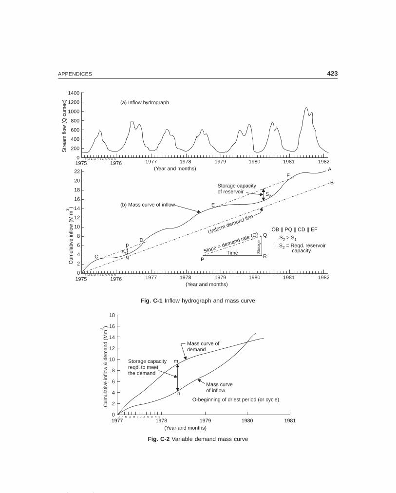
C-9\N-HYDRO\APP-1.PM5 423
APPENDICES 423
J F M A M J J A S O N D
1975 1976 1977 1978 1979 1980 1981 1982(Year and months)
J F M A M J J A S O N D
1975 1976 1977 1978 1979 1980 1981 1982(Year and months)
Slope = demand rate (Q) Q
RP
Time Sto
rage
Uniform demand line
OB || PQ || CD || EF
S > S2 1
\ S = Reqd. reservoircapacity
2
S2
Storage capacityof reservoir
E
F
(b) Mass curve of inflow
C
Dp
S1
22
20
18
16
14
12
10
8
6
4
2
0
Cum
ulat
ive
inflo
w(M
m)3
Str
eam
flow
(Qcu
mec
)
1400
1200
1000
800
600
400
200
0
(a) Inflow hydrograph
A
B
Fig. C-1 Inflow hydrograph and mass curve
J F M A M J J A S O N D
1977 1978 1979 1980 1981(Year and months)
18
16
14
12
10
8
6
4
2
0
Cum
ulat
ive
inflo
w&
dem
and
(Mm
)3
Storage capacityreqd. to meetthe demand
Mass curve ofdemand
Mass curveof inflow
O-beginning of driest period (or cycle)
m
n
Fig. C-2 Variable demand mass curve
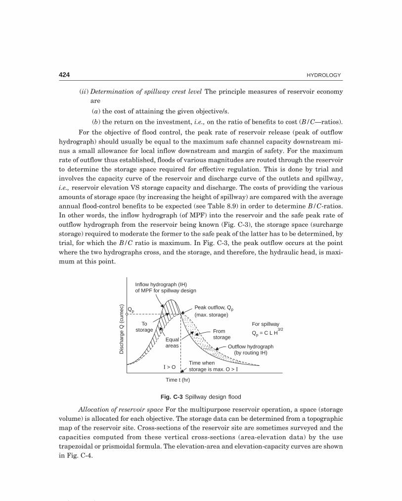
C-9\N-HYDRO\APP-1.PM5 424
424 HYDROLOGY
(ii) Determination of spillway crest level The principle measures of reservoir economyare
(a) the cost of attaining the given objective/s.
(b) the return on the investment, i.e., on the ratio of benefits to cost (B/C—ratios).
For the objective of flood control, the peak rate of reservoir release (peak of outflowhydrograph) should usually be equal to the maximum safe channel capacity downstream mi-nus a small allowance for local inflow downstream and margin of safety. For the maximumrate of outflow thus established, floods of various magnitudes are routed through the reservoirto determine the storage space required for effective regulation. This is done by trial andinvolves the capacity curve of the reservoir and discharge curve of the outlets and spillway,i.e., reservoir elevation VS storage capacity and discharge. The costs of providing the variousamounts of storage space (by increasing the height of spillway) are compared with the averageannual flood-control benefits to be expected (see Table 8.9) in order to determine B/C-ratios.In other words, the inflow hydrograph (of MPF) into the reservoir and the safe peak rate ofoutflow hydrograph from the reservoir being known (Fig. C-3), the storage space (surchargestorage) required to moderate the former to the safe peak of the latter has to be determined, bytrial, for which the B/C ratio is maximum. In Fig. C-3, the peak outflow occurs at the pointwhere the two hydrographs cross, and the storage, and therefore, the hydraulic head, is maxi-mum at this point.
Peak outflow, Q(max. storage)
p
Fromstorage
Outflow hydrograph(by routing IH)
For spillway
Q = C L Hp3/2
Inflow hydrograph (IH)of MPF for spillway design
Tostorage
Equalareas
I > O
Time t (hr)
Time whenstorage is max. O > I
Dis
char
geQ
(cum
ec)
Qp
Fig. C-3 Spillway design flood
Allocation of reservoir space For the multipurpose reservoir operation, a space (storagevolume) is allocated for each objective. The storage data can be determined from a topographicmap of the reservoir site. Cross-sections of the reservoir site are sometimes surveyed and thecapacities computed from these vertical cross-sections (area-elevation data) by the usetrapezoidal or prismoidal formula. The elevation-area and elevation-capacity curves are shownin Fig. C-4.

C-9\N-HYDRO\APP-1.PM5 425
APPENDICES 425
6 1500 4 3 2 1 1000 9 8 7 6 500 4 3 2 1 0
560
550
540
530
520
510
500
490
480
470
460
4500 50 100 150 200 250 300 350 400
Capacity (Storage volume) (M.m )3
Ele
vn.a
bove
msl
(m)
Water spread area (ha)
550.00 TOB (TOD)546.50 HFL (MWL)542.50 SCLFRL 543.5
Elevn.-capacity curveElevn. area curve
500.00 LSL (DSL)
471.00 RBL
Fig. C-4 Elevation-area-capacity curves for reservoir (Example C-2)
The various control levels in the operation of a multi-purpose reservoir are shown inFig. C-5. Full reservoir level (FRL) is at the level of the spillway crest or top of the spillwaygate. Towards the end of the flood season, the spillway gates are kept closed to store waterupto the top of the gate. The spill of the gate is well below the FRL in order to reduce the totallength of the spillway (since the head over the crest becomes more) for the passage of thespillway design flood. The low reservoir level (LWL) is at the elevation of the lowest sluiceoutlet and the water stored below LWL is the dead storage where the silt carried by the streamaccumulates and is usually kept at a about 10% of the gross reservoir storage (GS). In the caseof hydroelectric projects, the LWL to be maintained is from the point of minimum head re-quired for the operating efficiency of the turbines and to supply firm power (i.e., the poweravailable all the year round ; power available during a part of the year is called secondarypower and has to be sold at a much lower rate or firmed by thermal installation). The storagevolume between the FRL and LWL is called the useful storage, which can further be dividedinto conservation storage and flood control storage, according to the plan of operation of thereservoir. With an adequate flow forecasting system, all or part of the reservoir storage belowFRL (say, between FRL and an intermediate reservoir level IRL) can also be made availablefor flood control and multi-purpose regulation.
During normal flows, the reservoir level will be maintained in the vicinity of FRL andthe water will pass through the power conduits. Whenever a flood is forcest, the FRL isdrawndown to the extent that the flood runoff will bring the reservoir back to FRL. During lowflows, when FRL is reached, the release for power and downstream water requirements will bereduced to minimum.

C-9\N-HYDRO\APP-1.PM5 426
426 HYDROLOGY
HHPower conduit
Sluiceway Powerhouse
H = min. headfor firm power
Spillwaygates
550.00 –TOD
Spillwaycrest
546.50 MWL
543.50 FRL542.50 SCL
Surcharge storage
Conservation storage
500.00 LSL/LWL
Seasonalvariation
of resv. level
Valley storageRBL 471.00
River bedHeightof dam = 79m
Low waterseason
Low waterseason
M A M F J D N O S AMonths Flood months
season
JDNOSAJJMA
T
T TurbineTWL Tail water level
TWL
Fig. C-5 Multipurpose reservoir operation (Example C-2)
During high floods, the reservoir level will rise above FRL or well above the spillwaycrest level. The storage volume between this maximum reservoir level (MWL) and the FRL iscalled the surcharge storage, which exists only during a flood (where the spillway gates areopened to pass the flood water) and can not be retained for later use. When the floods subside,again the spillway gates are closed to conserve water upto FRL. The spillway has to pass thedesign flood with the head H = MWL—FRL.
Water stored during floods in the permeable banks of the reservoir is called ‘bank stor-age’ and drains out when the water level is lowered. The water stored in a natural stream-channel is called ‘valley storage’ and is a variable volume. From the point of flood control, theeffective storage in the reservoir = useful storage + surcharge storage – natural valley storage.
In the case of shallow and narrow rivers, the velocity will be high ; the water surfaceduring high flows may be steep (with considerable amount of wedge storage) and the watersurface profile (back water curve) can be computed by the non-uniform flow equation (for agiven inflow rate and the reservoir elevation at the dam). Fron this the information regardingthe water surface levels at various points along the stream, submergence of lands, roads, bridges,and other strategic structures for which compensation has to be paid, the acquisition of lands,etc., can be obtained.Example C-1 (a) The runoff data for a river during a lean year along with the probable de-mands are given below. Can the demands be met with the available river flow ? If so, how ?
(b) What is the maixmum uniform demand that can be met and what is the storagecapacity required to meet this demand ?
Month : J F M A M J J A S O N DRiver flow(Mm3) 135 23 27 21 15 40 120 185 112 87 63 42Demand(Mm3) 60 55 80 102 100 121 38 30 25 59 85 75
Solution (a) Evaporation losses and the prior water rights of the downstream user are notgiven and hence not considered. The computation is made in Table C-1. Since the cumulativesurplus is more than the cumulative deficit the demands can be met with the available riverflows, by constructing a reservoir with minimum storage capacity of 352 Mm3, which is also
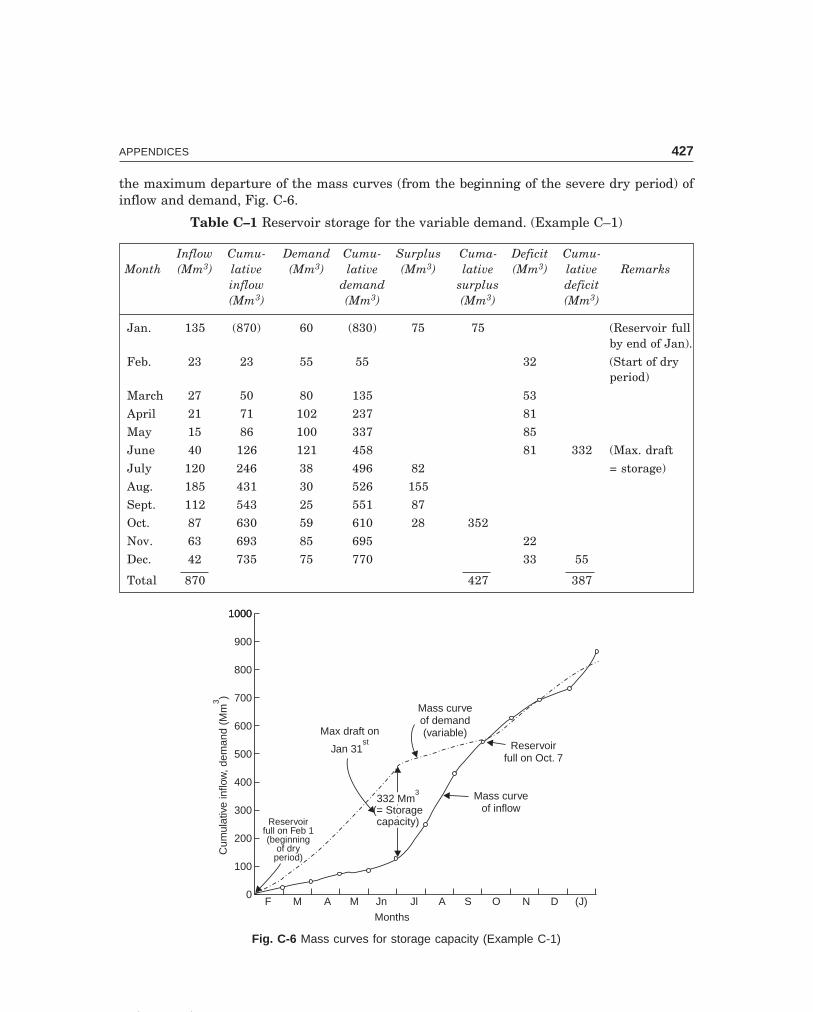
C-9\N-HYDRO\APP-1.PM5 427
APPENDICES 427
the maximum departure of the mass curves (from the beginning of the severe dry period) ofinflow and demand, Fig. C-6.
Table C–1 Reservoir storage for the variable demand. (Example C–1)
Inflow Cumu- Demand Cumu- Surplus Cuma- Deficit Cumu-Month (Mm3) lative (Mm3) lative (Mm3) lative (Mm3) lative Remarks
inflow demand surplus deficit(Mm3) (Mm3) (Mm3) (Mm3)
Jan. 135 (870) 60 (830) 75 75 (Reservoir fullby end of Jan).
Feb. 23 23 55 55 32 (Start of dryperiod)
March 27 50 80 135 53
April 21 71 102 237 81
May 15 86 100 337 85
June 40 126 121 458 81 332 (Max. draft
July 120 246 38 496 82 = storage)
Aug. 185 431 30 526 155
Sept. 112 543 25 551 87
Oct. 87 630 59 610 28 352
Nov. 63 693 85 695 22
Dec. 42 735 75 770 33 55
Total 870 427 387
Reservoirfull on Feb 1(beginning
of dryperiod)
332 Mm(= Storagecapacity)
3332 Mm
(= Storagecapacity)
3 Mass curveof inflow
Reservoirfull on Oct. 7
Mass curveof demand(variable)Max draft on
Jan 31st
Cum
ulat
ive
inflo
w, d
eman
d(M
m)3
1000
900
800
700
600
500
1000
400
300
200
100
0F M A M Jn Jl
Months
A S O N D (J)
Fig. C-6 Mass curves for storage capacity (Example C-1)

C-9\N-HYDRO\APP-1.PM5 428
428 HYDROLOGY
In the bar graph (Fig. C-7), the monthly inflow and demand are shown by full line anddashed line, respectively. The area of maximum deficit (i.e., demand over surplus) is the stor-age capacity required and is equal to 332 Mm3.
SurplusSurplusSurplusSurplus
(b) 276.5 Mm= Storage reqd.
(to meet the uniformdemand)
3
Monthlydemand
(a) Deficit= Storage
332 M.m3
Uniform demand
of 725 M.m3
Monthly inflow
InflowDemand (variable)Uniform demand
J F M A M Jn A S O N D
(Months)
200
160
120
80
40
0
Inflo
w,D
eman
d(M
m)3
Jl
Fig. C-7 Bar-graph for storage capacity (Example C-1)
(b) The cumulative inflow in the lean year is 870 Mm3. The maximum uniform demand
that can be met is 87012
= 72.5 Mm3 per month. In the bar graph (Fig. C-7), the line of uniform
demand is drawn at 72.5 M.m3/month. The shaded area represents the surplus over the uni-form demand (during the months of January, and July to October), which is the storage capac-ity required to meet the uniform demand, and is equal to
(135) + (120 + 185 + 112 + 87) – 72.5 × 5 = 276.5 Mm3
Example C-2 The following are the data for a proposed medium size reservoir inMaharashtra. Determine LSL, FRL, HFL (MWL). What is the total length of the spillway fittedwith crest gates assuming a pier width of 1.5 m (10 m span), flood detention of 4 hr and C = 2.2.
Catchment area 1200 km2
Rainfall of 75% dependability 900 mmGross commanded area 25000 ha
Crpping pattern (proposed) and their water requirement (∆)(i) Kharif : Jowar—30% (0.45 m), Cotton—15% (0.75 m),
Rice—10% (1.20 m), Sugar cane—10% (1.90 m)(ii) Rabi: Rice—20% (1.20 m), Wheat—20% (0.45 m)
(iii) Hot Weather: Vegetables—20% (0.60 m)Area Capacity of Reservoir Site
Contour RL (m) 471 475 495 500 505Area (ha) 0 36 178 242 323
Capacity (Mm3) 0 0.90 19.35 29.85 43.98

C-9\N-HYDRO\APP-1.PM5 429
APPENDICES 429
Contour RL (m) 530 535 540 545
Area (ha) 841 1002 1224 1480Capacity (Mm3) 186.62 232.69 288.34 355.95
River bed level 471.0Top of bund level (TBL) 550.0
Silt load (expected) 250 m3/km2/yr with a life of 100-yr.Evaporation losses 1.5 m over the mean area
Empirical formula for yield andflood of the region Inglis formula.Solution (a) Yield from the basin :
Dependable runoff R = ( . )P P− 17 8
254Inglis formula
P = 95 cm, R = ( . )90 17 8 90
254−
= 25.6 cm
Yield = AR = 1200 × 106 (0.256) = 307.2 × 10⁶ m3
= 307 Mm3.(b) Irrigation water requirement:
(i) Kharif: Jowar 25000 × 0.3 × 0.45 = 3380 ha-mCotton 25000 × 0.15 × 0.75 = 2820 ha-mRice 25000 × 0.10 × 1.20 = 3000 ha-mSugarcane 25000 × 0.10 × 1.90 = 4750 ha-m
13950 ha-m
(ii) Rabi: Rice 25000 × 0.20 × 1.20 = 6000 ha-mWheat 25000 × 0.20 × 0.45 = 2250 ha-m
8250 ha-m(iii) Hot weather:
Vegetables 25000 × 0.20 × 0.60 = 3000 ha-mTotal for the three crop seasons = 25200 ha-m.Allowing 20% for conveyance losses, 10% for evaporation and seepage losses in the res-
ervoir, 5% for overlap, and 5% as carryover storage—a total of 40%.Live storage = 25200 × 1.40 = 35280 ha-m or = 352.8 Mm3
While the annual yield is only 307 Mm3 which limits the area irrigated unless supple-mented by natural rainfall. Hence, a live storage of 307 M.m3 is possible. Curves of eleven. vs.capacity and eleven. vs. water spread area are shown in Fig. C-4.
Dead storage = 250 × 1200 × 100 = 30 × 106 m3 or 30 Mm3
for which from the elevn-capacity curve, the lowest sill level of the sluice, LSL = 500.00 mGross storage = Dead storage + Live storage = 30 + 307 = 337 Mm3
for which from the elevn-capacity curve, the full reservoir levelFRL = 543.50 m

C-9\N-HYDRO\APP-1.PM5 430
430 HYDROLOGY
Allowing a flood lift of 3 m, the maximum water level (MWL) orHFL = 546.50 m
With a freeboard of 3.5 m, top of bound level or top of dam, TBL orTOD = 550.00 m
Height of dam = TOD – RBL = 550.00 – 471.00 = 79 m
Length of spillwayAssuming the crest of the spillway is at FRL, the head on the spillway.
HFL – FRL = 546.5 – 543.5 = 3 mEffective length of spillway per span
Le = L – 0.1 nH= 10 – 0.1 × 2 × 3 = 9.4 m
Discharge over spillway per spanq = CLe H
3/2
= 2.2 × 9.4 × 33/2 = 108 cumec/spanFlood absorbing capacity
FAC = Capacity at HFL – capacity at FRL = 374–337 = 37 Mm3
Spillway design flood, QD = MPF – FAC
T
where T = flood detention time in the reservoir and usually varies between 2 12 to 16 hr, and
here given as T = 4 hr. The maximum flood discharge (MPF) may be calculated from the Inglisformula applicable for the region.
MPF ≈ 124
10 24
A
A + .
≈ 124 1200
1200 10 24
×− .
≈ 4280 cumec
∴ QD = 4280 – 37 10
4 60 60
6×× ×
= 1710 cumec
∴ No. of spans required = 1710108
= 15.8, say, 16.
Total length of spillway = 16 × 10 + 1.5 × 15 spans piers= 182.5 m
This length of the spillway can be reduced if the spillway crest (i.e., the sill of the crestgates) is kept at R.L. 542.50 m, so that the crest gates (height = 4 m) conserve water upto R.L.543.50 m (FRL) or even above this level, as the floods subside (i.e., towards the end of floodseason).
H = 546.5 – 542.5 = 4 m
C-9\N-HYDRO\APP-1.PM5 431
APPENDICES 431
q = 2.2 × 9.4 × 43/2 = 165.5 cumec/spanFAC = 374 – 322.5 = 51.5 M.m3
(since when the floods are forecast, the FRL is lowered to the spillway crest level by openingthe crest agates)
QD = 4280 – 515 104 60 60
6. ×× ×
= 700 cumec
No. of spans required = 700
165 5. = 4.23, say 5 spans
Total length of spillway = 5 × 10 + 1.5 × 4 = 56 mThe various control levels are shown in Fig. C-5.The flood absorption capacity thus reduces the peak of the MPF. Actually the MPF
hydrograph into the reservoir (inflow hydrograph) is first obtained and then routed (for anassumed elevn of spillway crest, RL of sluice outlets) by making use of elevn-capacity-dis-charge relationship, and the peak of the outflow hydrograph thus derived gives the spillwaydesign flood. For small reservoirs (catchment area < 100 km2) the flood absorbing capacity isneglected as additional safety factor.
Assignment Problem
For the peak of the outflow hydrograph obtained by routing (by modified Puls method) thehydrograph of inflow into the reservoir in Example 9.1, determine the length of spillway assumingC = 2.2 (Note: Max. pool elevn. reached = 113.6 m, and elevn. of spillway crest = 112.3 m).

When a well in an extensive confined aquifer is pumped at a constant rate, water isreleased from storage within the aquifer due to decompression as the piezometric head isreduced and the radius of influence increases, with respect to time. Assuming that the velocityof flow in the aquifer as horizontal, the differential equation in polar coordinates can be writtenas
∂∂
∂∂
2
21h
r rhr
+ = ST
hr
∂∂
...(1)
Using the analogy of the above equation to heat conduction, Theis (1935) obtained thefollowing solution by assuming that h = H at t = 0, and after pumping (at a constant rate Q)starts, h → H as r → ∞. The drawdowns at any distance r from the pumping well is given by
s = H – h = Q
Teuu
u
4π
∞ −z du ...(2)
or, s = Q
T4π W(u) ...(3)
and, u = r S
Tt
2
4...(4)
W(u) is called the well function and u is called the argument of the well function ; T andS are the aquifer constants called the transmissibility and storage coefficients. The solution ofEq. (2) is
s = Q
T4π − − + − + − +LNM
OQP0 577216
2 2 3 3 4 4
2 3 4
. ln. ! . ! . !
......u uu u u
...(5)
The convergent series in brackets is the well function W(u). Both u and W(u) aredimensionless and the plot of W(u) vs. u on log-log paper is called the ‘Theis Type Curve’(Fig. D-1). The values of W(u) for different values of u are given in Tables (Ferris et al., 1962).Since W(u) and u are both functions of T and S, Eqs. (3) and (4) can not be solved directly andspecial procedures are employed.
Appendix D
UNSTEADY GROUNDWATER FLOW
432

C-9\N-HYDRO\APP-1.PM5 433
APPENDICES 433
W(u) vs. uW(u) vs. u
W(u)
v
10
5
2
1
5
2
0.110
–410
–32 5 2 5 2 510
–22 510
–11
Fig. D-1 Theis Type-curve for the well function
(a) Theis’ Graphical Procedure (Theis 1935, Lohman, 1972)Taking logarithms of Eq. (3),
log s = log Q
T4π + log W(u) ...(6)
From Eq. (4), rt
2
= 4Tu
S...(7)
and taking logarithms of Eq. (7),
log rt
2
= log 4TS
+ log u ...(8)
Since QT4π
and 4TS
are constants for a particular pumping test, the Eqs. (6) and (8) are
similar. If the field pump-test curve ‘s vs. rt
2
’ and the ‘type curve’ ‘W(u)’ vs. u are drawn to the
same scale on log-log paper on separate transparent sheets and superimposed with thecoordiante axes parallel, so that the two curves coincide for some length AB, an arbitrarymatch point P is selected, Fig. D-2, and its coordinates are read on both the graphs. From the
match-point coordinates, s, rt
2
, W(u), and u, the aquifer constants can be calculated from Eqs.
(3) and (4).(b) Cooper-Jacob Solution (Modified Theis)
From Eq. (4), it is evident that ‘u’ decreases as the pumping time t increases. Jacob(1946, 1950) pointed out that for large values of t and small values of r, u becomes smallenough so that in the convergent series, Eq. (5), the terms after the first two become negligible.Thus, the drawdown can be expressed as,
s = Q
T4π − −FHG
IKJ0 577216
4
2
. lnr S
Tt
after changing into logarithm to base 10 and simplifying
s = 2 34
2 252
.log
.QT
Ttr Sπ , u < 0.01 ...(9)
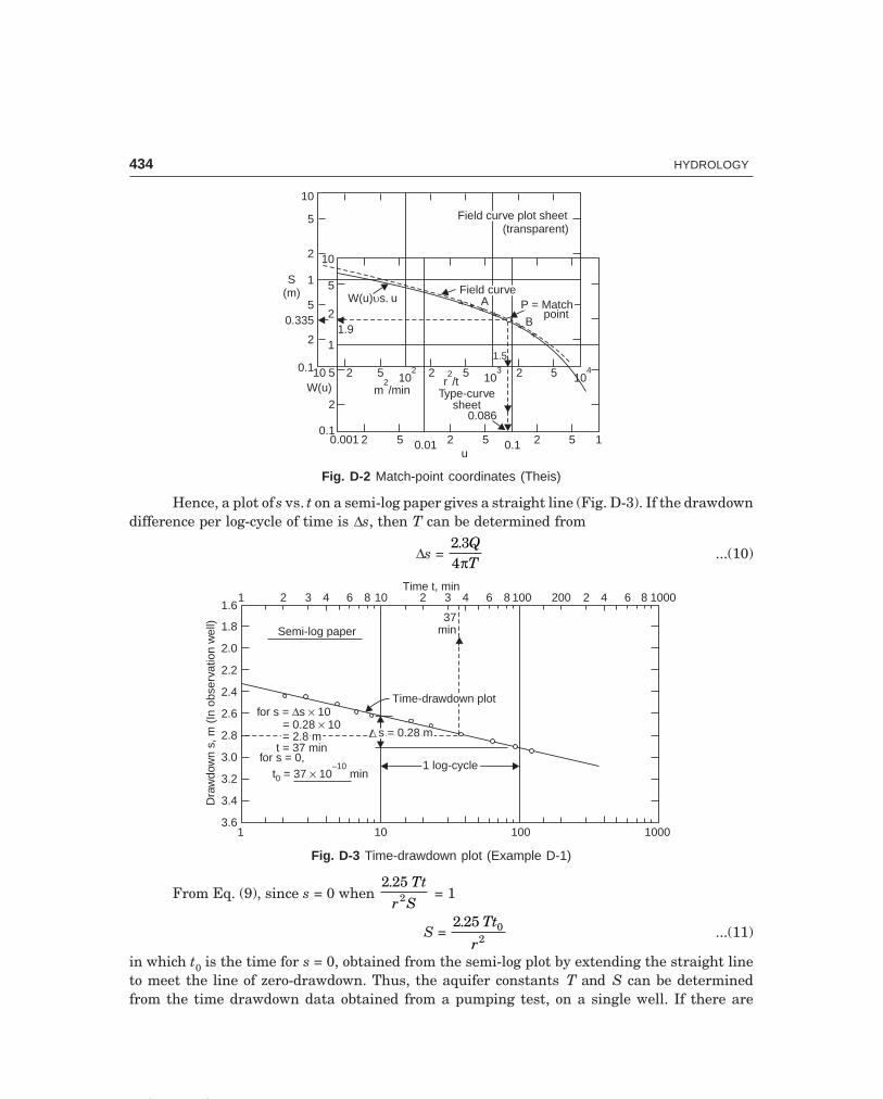
C-9\N-HYDRO\APP-1.PM5 434
434 HYDROLOGY
P = MatchP = Match
BB
AAField curveField curve
W(u) s. uuW(u) s. uu
1.9
1.5
m /min2
Type-curvesheet
r /t2
Field curve plot sheet(transparent)
Field curve plot sheet(transparent)
10
5
2
1
5
2
0.335
S(m)
10
5
2
1
0.1 510
2
0.1
W(u)2 5 10
2 2 5 2 5103
104
0.086
0.001 2 5 2 50.01 0.1u
2 5 1
point
Fig. D-2 Match-point coordinates (Theis)
Hence, a plot of s vs. t on a semi-log paper gives a straight line (Fig. D-3). If the drawdowndifference per log-cycle of time is ∆s, then T can be determined from
∆s = 2 34. Q
Tπ...(10)
Time-drawdown plotTime-drawdown plot
��s = 0.28 ms = 0.28 m
1 log-cycle1 log-cycle
for s = s 10= 0.28 10= 2.8 m
t = 37 min
� ��
for s = s 10= 0.28 10= 2.8 m
t = 37 min
� ��
for s = 0,t = 37 10 min0 �
–10for s = 0,
t = 37 10 min0 �–10
Semi-log paper
1.6
1.8
2.0
2.2
2.4
2.6
2.8
3.0
3.2
3.4
3.61 10 100 1000
100086422001008643210864321Time t, min
37min
Dra
wdo
wn
s,m
(In
obse
rvat
ion
wel
l)
Fig. D-3 Time-drawdown plot (Example D-1)
From Eq. (9), since s = 0 when 2 25
2. Tt
r S = 1
S = 2 25 0
2
. Tt
r...(11)
in which t0 is the time for s = 0, obtained from the semi-log plot by extending the straight lineto meet the line of zero-drawdown. Thus, the aquifer constants T and S can be determinedfrom the time drawdown data obtained from a pumping test, on a single well. If there are

C-9\N-HYDRO\APP-1.PM5 435
APPENDICES 435
several observation wells, by knowing their drawdown after pumping for a certain time t, theaquifer constants T and S can be determined by a plot of a distance-drawdown on a semi-logpaper (Fig. D-4). From Eq. (9),
s = 2 34
1
2
2.
logQT
rrπ
FHG
IKJ
Semi-log paper
1 log-cycle1 log-cycle
s = 3.25 ms = 3.25 mÑ
r = 210 m for s = 00r = 210 m for s = 00
1 2 3 4 6 8 10 2 3 4 6 8100 2 3 4 6 81000Distance of observation well r (m)
0
0.5
1.0
1.5
2.0
2.5
3.0
3.5
4.0
4.5
5.0
5.5
6.0
Dra
wdo
wn
inob
serv
atio
nw
ell,
s(m
)
1 10 100 1000
Fig. D-4 Distance drawdown plot (Example D-2)
If the drawdown difference per log-cycle of r is ∆s, then T can be determined from
Eq.(10): ∆s = 2 34. Q
Tπ...(12)
and S from
Eq.(11): S = 2 25
02
. Tt
r...(13)
where r0 is the distance for s = 0 obtained by extending the straight line plot to meet the line ofzero drawdown.(c) Theis’ Recovery Method
If a well is pumped for a time t1 (when the drawdown is s1) and then stopped, thedrawdown goes on decreasing. The residual drawdown s′, at time t′ since pumping stopped, ort since pumping started (t = t1 + t′), is equal to the drawdown (s) due to continuous pumpingupto t, minus increase in head (sr) due to an equal recharging well since pumping stopped(Fig. D-5), i.e.,
s′ = s – sr ...(14)For small r and large t′,
s′ = 2 34.
logQT
ttπ ′
, u < 0.01 ...(15)
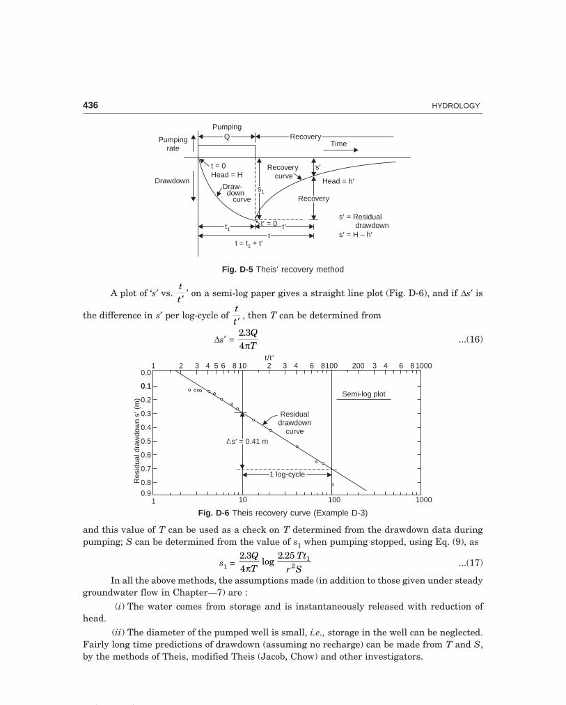
C-9\N-HYDRO\APP-1.PM5 436
436 HYDROLOGY
Head = h¢
s¢
RecoveryRecovery
s = Residualdrawdown
= H – h
¢
¢ ¢s
Recoverycurve
Recoverycurve
s1s1
t = 0Head = H
Draw-down
curve
QQ RecoveryRecoveryTimePumping
rate
Drawdown
t¢t¢t1t1tt
t = 0¢
t = t + t1 ¢
Pumping
Fig. D-5 Theis’ recovery method
A plot of ‘s′ vs. tt ′
’ on a semi-log paper gives a straight line plot (Fig. D-6), and if ∆s′ is
the difference in s′ per log-cycle of tt ′
, then T can be determined from
∆s′ = 2 34. Q
Tπ...(16)
0.0
0.1
0.2
0.3
0.4
0.5
0.6
0.1
0.7
0.8
0.9
Res
idua
ldra
wdo
wn
s(m
)¢
1 2 3 4 5 6 8 10 2 3 4 6 8100 200 3 4 6 8 1000
100010010
1 log-cycle1 log-cycle
s = 0.41 m¢s = 0.41 m¢Ñ
Residualdrawdown
curve
Semi-log plot
t/t¢
1
Fig. D-6 Theis recovery curve (Example D-3)
and this value of T can be used as a check on T determined from the drawdown data duringpumping; S can be determined from the value of s1 when pumping stopped, using Eq. (9), as
s1 = 2 34
2 25 12
.log
.QT
Tt
r Sπ ...(17)
In all the above methods, the assumptions made (in addition to those given under steadygroundwater flow in Chapter—7) are :
(i) The water comes from storage and is instantaneously released with reduction ofhead.
(ii) The diameter of the pumped well is small, i.e., storage in the well can be neglected.Fairly long time predictions of drawdown (assuming no recharge) can be made from T and S,by the methods of Theis, modified Theis (Jacob, Chow) and other investigators.

C-9\N-HYDRO\APP-1.PM5 437
APPENDICES 437
Example D-1 A 200 mm-well is pumped at the rate 1150 lpm. The drawdown data on anobservation well 12.3 away from the pumped well are given below. Determine the transmissi-bility and storage coefficients of the equifer. What will be the drawdown at the end of 180 days(a) in the observation well, (b) in the pumped well ? Use the modified Theis method ; underwhat conditions is this method valid ?
Time (min): 2 3 5 7 9 12
Drawdown (m): 2.42 2.46 2.52 2.58 2.61 2.63
Time (min): 15 20 40 60 90 120
Drawdown (m): 2.67 2.71 2.79 2.85 2.91 2.94
Solution The time-drawdown plot is shown in Fig. D-3, from which ∆s = 0.28 m per log-cycleof t, and t0 (for s = 0) is 37 × 10–10 min.
∴ T = 2 34
2 3 1150 604 0 28
. . . /( . )
Qsπ∆ π
= × = 0.0125 m2/s
or 10.8 × 10⁵ lpd/m
S = 2 25 0
2
. Tt
r =
2 25 0 0125 10 60
12 3
10
2
. ( . )37
( . )× ×−
= 4.12 × 10⁻¹¹
(a) Drawdown in the observation well after 180 days,
s = 2 34
2 252
.log
.QT
Tt
r Sπ , u < 0.01
s = 2 3 1150 604 0 0125
2 25 0 0125 180 86400
12 3 4 12 102 11. ( . / )
( . )log
. ( . )
( . ) .π×
× − = 3.89 m
(b) Drawdown in the pumped well after 180 days
sw = 2 3 1150 604 0 0125
2 25 0 0125 180 864000 100 4 2 102 11
. ( . / )( . )
log. ( . )
( . ) .π×
× − = 5.06 m.
The Jacob’s method is valid for u < 0.01
r STt
2
4 < 0.01
or t > r S
T
2
0 04. >
( . ) .. ( . )
12 3 4 12 100 04 0 0125
2 11× − > 1.25 × 10⁻⁵ sec
i.e., instantaneously after pumping starts.Example D-2 A production well was pumped for 2 hr at a constant rate of 1600 lpm and thedrawdowns in the seven nearby observation wells are given below. Determine the aquifer con-stants S and T.
Observation well A B C D E F G
Distance from pumped well (m) 5 10 20 40 80 120 200
Drawdown (m) 5.35 4.35 3.35 2.35 1.4 0.8 0.3

C-9\N-HYDRO\APP-1.PM5 438
438 HYDROLOGY
Solution The distance-drawdown plot is shown in Fig. D-4 from which ∆s = 3.25 m per log-cycle of r, and r0 (for s = 0) is 210 m.
T = 2 32
2 3 1600 602 3 25
. . ( . / )( . )
Qsπ∆ π
= = 0.003 m2/s for 2.6 × 10⁶ lpd/m
S = 2 25 2 25 0 03 2 60 60
21002 2
. . ( . )Tt
r=
× × = 0.0011
Example D-3 A 400-mm well was pumped at the rate of 2000 lpm for 200 min and the drawdownin an observation well 20 m from the pumping well was 1.51 m. The pumping was stopped andthe residual drawdowns during recovery in the observation well for 2 hr are given below. Deter-mine the aquifer constants S and T.
Time since Residual Time since Residualpumping stopped drawdown pumping stopped drawdown
(min) (m) (min) (m)
2 0.826 45 0.180
3 0664 50 0.159
5 0.549 55 0.155
10 0.427 60 0.149
16 0.351 70 0.146
20 0.305 80 0.140
25 0.271 90 0.134
30 0.241 100 0.131
35 0.220 110 0.131
40 0.201 120 0.131
Solution The time-residual drawdown data are processed in Table D-1 and the Theis recoverycurve is plotted on a semi-log paper as shown in Fig. D-6.
Table D-1 Theis recovery method, t1 = 200 min.
Time since Residual Time since pumping Ratiopumping stopped drawdown started t = t1 + t′ (t/t′)
t′ (min) s′ (m) (min)
2 0.826 202 101
3 0.664 203 68
5 0.549 205 41
10 0.427 210 21
16 0.351 216 13.5
20 0.305 220 11
25 0.271 225 9
30 0.241 230 7.7
35 0.220 235 6.7
40 0.201 240 6
(Contd.)...

C-9\N-HYDRO\APP-1.PM5 439
APPENDICES 439
45 0.180 245 5.45
50 0.159 250 5
55 0.155 255 4.65
60 0.149 260 4.33
70 0.146 270 3.86
80 0.140 280 3.5
90 0134 290 3.22
100 0.131 300 3.00
110 0.131 310 2.82
120 0.131 320 2.66
From the recovery plot, ∆s′ = 0.41 m per log-cycle of t/t′ and
T = 2 34
2 3 2 000 604 0 41
. . ( . / )( . )
Qsπ∆ π′
= = 0.0149 m2/s
= 1.284 × 10⁶ lpd/m,and S can be obtained from s1 = 1.51 m after 200 min of pumping as
s1 = 2 34
2 25 12
.log
.QT
Ttr Sπ
log 2 25 4 0 0149 151
2 3 2 000 601
2. ( . ) .
. ( . / )Tt
r S= π
= 3.69
Antilog of 3.69 = 48982 25 0 0149 200 60
202. ( . ) ×
S = 4898
∴ S = 0.000206
Ground Water ExtractionExcessive lowering of the groundwater table by pumping may result in crop failures, depletionof a nearby stream by increased percolation losses, salt water intrusion in coastal aquifers,and occasionally serious settlement of the ground surface.
The natural recharging of ground water regimen can be supplemented by ponding orwater spreading. For confined aquifers or shallow beds where ponding is not practicable, re-charging is affected by pumping water down the wells at rates rather less than the correspond-ing withdrawal rates. Mostly recharge water is excess surface water, but industrial wastewater, sewage and uncontaminated cooling water from industrial and airconditioning plantsare used in some countries.
Sea water intrusion in coastal aquifers occurs when permeable formations out crop intoa body of sea water and when there is landward gradient. Intrusion can be controlled by reduc-ing pumping, by increasing supply or by constructing a physical barrier.
There is need for legislation of groundwater extraction and regulation to check indis-criminate draining of groundwater resources. Precautions should be taken against pollution ofsurface and subsoil waters by enacting legislation.
Tube well schemes may be integrated with the canal irrigation schemes by suitablyspacing them along the drainage lines in the distribution area. The drainage system must beplanned as an integral part of the distribution system in the design stage itself. The drainage

C-9\N-HYDRO\APP-1.PM5 440
440 HYDROLOGY
water may be used again by pumping in double and triple cropping as is already in practice inKrishna and Godavari deltas.
For a detailed study of ground water i.e., Ground Water Survey, Geohydrology andTube Wells, and Irrigation Systems, reference may be made for the Author’s companion vol-ume ‘Ground Water – 3rd Edn.’ by the same Publisher.
Assignment Problems
1 A 300 mm production well tapping an artesian aquifer 30-m thick is continuously pumped atconstant rate of 100 m3/hr for 1 day and the drawdowns in an observation well at 80 m from thepumped well are given below. Compute the coefficients of transmissibility, permeability, andstorage of the aquifer. What is the drawdown in the pumping well after 180 days of continuouspumping assuming no recharge.
Time Drawdown Time Drawdown(min) (m) (min) (m)
1 0.14 60 0.70
2 0.22 80 0.75
3 0.27 100 0.80
4 0.31 300 0.83
6 0.34 500 1.00
7 0.38 700 1.03
8 0.40 900 1.06
10 0.43 1000 1.08
30 0.60 1440 1.14
(1375 m2/d, 45.8 m/d, 1.35 × 10⁻⁴, ...)
2 A 400-mm-production well penetrating a water table acquifer is pumped at a constant rate of100 m3/hr for a period of 200 days. The drawdowns in three observation wells are given below.Compute the coefficient of storage and transmissibility of the aquifier.
Observation Well A B C
Distance from pumping well (m) 2 20 200
Drawdown (m) 2.75 1.80 0.90
(977 m2/d, 0.11)

The hydrological methods of flood routing discussed in Chapter—9 were based on thecontinuity equation in a simplified finite form called the storage equation.
I = OSt
+ ∆∆
where I O, are the mean values of inflow and outflow, and ∆S is the increment in storage inperiod ∆t.
Flows and elevations within a reservoir were not directly determined but estimatedfrom flow profiles and rating curves.
A more mathematical method exists, based on the principle of continuity (law of conser-vation of mass) and energy principle (law of conservation of energy), which permit computa-tion of stage or discharge hydrographs at any point in the stream, as well as the water surfaceprofile at any time. The basic differential equations for gradually varied unsteady flow in openchannels are
Continuity eqn. : B ∂∂Ht
+ ∂∂
( )AVx
= q ...(2)
Energy eqn. : ∂∂Vt
+ V ∂∂Vx
+ VA
q = g S Syxf0 − −F
HGIKJ
∂∂
...(3)
where H = water surface elevationx = distance along channel
B = width of channel at water surface S0 = bed-slope of channel Sf = friction slope t = time y = depth of flow V = velocity of flow q = local inflow into channel per unit widthBy selecting finite time and space differences and assuming boundary conditions,
numerical solutions of the above basic differential equations can be made by the use of electronic
Appendix E
FLOOD ROUTING BY
CHARACTERISTIC CONCEPTS
441
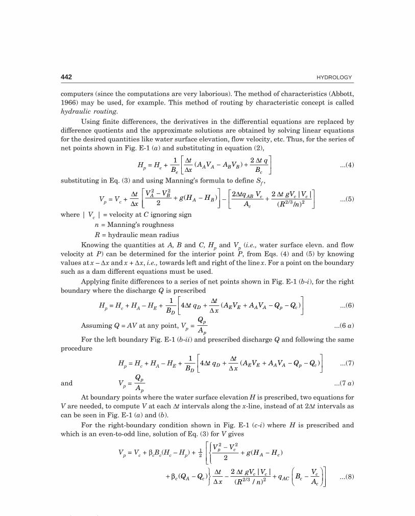
C-9\N-HYDRO\APP-2.PM5 442
442 HYDROLOGY
computers (since the computations are very laborious). The method of characteristics (Abbott,1966) may be used, for example. This method of routing by characteristic concept is calledhydraulic routing.
Using finite differences, the derivatives in the differential equations are replaced bydifference quotients and the approximate solutions are obtained by solving linear equationsfor the desired quantities like water surface elevation, flow velocity, etc. Thus, for the series ofnet points shown in Fig. E-1 (a) and substituting in equation (2),
Hp = He + 1 2
Btx
A V A Vt q
BeA A B B
c
∆∆
∆( )− +
LNM
OQP
...(4)
substituting in Eq. (3) and using Manning’s formula to define Sf ,
Vp = Vc + ∆∆
tx
V V
g H HA BA B
2 2
2−
+ −LNMM
OQPP
( ) – 2 2
2 3 2
∆ ∆tq VA
t gV VR n
AB c
c
c c+LNM
OQP
| |
( / )/ ...(5)
where | Vc | = velocity at C ignoring sign n = Manning’s roughness R = hydraulic mean radiusKnowing the quantities at A, B and C, Hp and Vp (i.e., water surface elevn. and flow
velocity at P) can be determined for the interior point P, from Eqs. (4) and (5) by knowingvalues at x – ∆x and x + ∆x, i.e., towards left and right of the line x. For a point on the boundarysuch as a dam different equations must be used.
Applying finite differences to a series of net points shown in Fig. E-1 (b-i), for the rightboundary where the discharge Q is prescribed
Hp = Hc + HA – HE + 1
4B
t qtx
A V A V Q QD
D E E A A p c∆∆∆
+ + − −LNM
OQP
( ) ...(6)
Assuming Q = AV at any point, Vp = Q
Ap
p...(6 a)
For the left boundary Fig. E-1 (b-ii) and prescribed discharge Q and following the sameprocedure
Hp = Hc + HA – HE + 1
4B
t qtx
A V A V Q QD
D E E A A p c∆∆∆
+ + − −LNM
OQP
( ) ...(7)
and Vp = Q
Ap
p...(7 a)
At boundary points where the water surface elevation H is prescribed, two equations forV are needed, to compute V at each ∆t intervals along the x-line, instead of at 2∆t intervals ascan be seen in Fig. E-1 (a) and (b).
For the right-boundary condition shown in Fig. E-1 (c-i) where H is prescribed andwhich is an even-to-odd line, solution of Eq. (3) for V gives
Vp = Vc + βcBc(Hc – Hp) + 12
V Vg H Hp c
A c
2 2
2
−+ −
RS|T|L
NMM ( )
+ − UVW− + −
FHG
IKJOQPP
βc A cc c
AC cc
cQ Q
tx
t gV VR n
q BVA
( )| |
( / )/
∆∆
∆22 3 2 ...(8)

C-9\N-HYDRO\APP-2.PM5 443
APPENDICES 443
A B
P
C
t
t – t
t – 2 tÑ
Ñ
Ñx
Ñx
Ñxx –
Ñxx +x
A
D
C
t
Ñx
Ñx
Ñx xx –
E
x – 2Ñ
x
P EP
C A
t
Ñxx +
Ñ2 xx +x
Ñx
Ñx
D
(a) Interior point P: Q-prescribed Eqs. (4) and (5) for H, V
(i) Right boundary point PEqs. (6) and (6a) for H, V
(ii) Left boundary point PEqs. (7) and (7a) for H, V
(b) Boundary points : Q-prescribed
t
CÑx
ÑxÑ
x xx –x – 2Ñ
A
P
(i) Right boundary point Peven to odd line Eq. (8) for V
t
t- tÑ
Ñx
Ñx
x x + 2x +Ñ
P
x
xÑ
x
(iii) Left boundary pointeven to odd line Eq. (8b) for V
t
CÑx
ÑxÑ
x xx –x – 2Ñ
A
P
x
(ii) Right boundary point Podd to even line Eq. (8a) for V
t
Ñx
Ñx
x x +Ñ
A
x
C
P
x + 2Ñ
x
(iv) Left boundary point Podd to even line Eq. (8c) for V
(b) Boundary points : H-prescribed
x
(d) The x-t plane
t
2 x2 xÑÑ
xxÑÑ
ÑÑt
ÑÑt
t-line
t-line1 2 3 4
5 6 7 8
9 10 11 12
13 14 15 16
17 18 19 20
t – t
t – 2 tÑ
Ñt – t
t – 2 tÑ
Ñ
t – tÑ
t – tÑ
t – tÑ
Fig. E-1 Net points in finite difference schemes

C-9\N-HYDRO\APP-2.PM5 444
444 HYDROLOGY
where βc = g
A Bc c
and for the right boundary odd-to-even line, with H prescribed, Fig. E-1 (c-ii), use Eq. (8)
with ∆∆
tx
replaced by 2 ∆∆
tx
...(8a)
At the left boundary even-to-odd line with H prescribed, Fig. E-1 (c-iii), use Eq. (8)
with βc replaced by – βc and∆∆
tx
by – ∆∆
tx
...(8 b)
and for the left-boundary odd-to-even line, with H prescribed, Fig. E-1 (c–iv) use Eq. (8)
with βc replaced by – βc and∆∆
tx
replaced by – 2 ∆∆
tx
...(8 c)
Because of the characteristics of the two basic differential equations used to derive Eqs.(4) to (8 c), a maximum permissible ratio for making the computations from time t to t + ∆t, isgiven by the inequality
∆∆
tx
≤ 1
V c+...(9)
where c is the celerity of small waves given by c = gym ,
where ym = mean depth of the river. For example, if ym = 10 m, V = 1.6 m/s, c = 9 81 10. × =
9.92 m/s and ∆∆
tx
< 0.087 s/m.
Computational ProcedureStarting with nearly steady conditions, Q and H must be known (or assumed) for all net pointsalong two consecutive t-lines, say point 1–8, in Fig. E-1 (d). Values of V (= Q/A) should becomputed for the points 1-8.
Suppose for the right boundary H is prescribed, and for the left boundary Q is pre-scribed. Based on the values of points 2, 5 and 6, values of H and V at point 10 can be computedby Eqs. (4) and (5). Similarly, H and V at point 11 can be computed based on values at points 3,6 and 7. This procedure can be continued for an indefinite number of interior points along thex-axis for a particular t-line.
At the left boundary where Q is presecribed using values at points 1, 2, 5 and 10, H atpoint 9 can be computed by Eq. (7) and V = Q/A.
At the right boundary where H is prescribed, using values at points 7 and 8, V at point12 can be computed by using odd-to-even line Eq. (8a). By using values at points 11 and 12, Vat point 16 can be computed by using even-to-odd line Eq. (8).
Following the above computational procedure, values of H and V at points on successivet-lines can be computed.
The product ∆x. ∆H gives changes in storage for the continuity equation. The Manning’sroughness ‘n’ can be determined from steady flow profiles. Local inflow can best be determinedby stream gauges on tributaries, and from rainfall using unit hydrographs.
Despite the difficulties in the determination of the parameters like A, R, n, c, etc., themethods that have been developed from the characteristic concepts have shown increasingutility.

The hydrologic equation is nearly a statement of the law of conservation of matter andis given by
Inflow = Outflow + ∆ Storagei.e., during a given time the total inflow to a given area must equal the total outflow plus thecharge in storage.
The items of inflow (into a basin or sub-basin) are :(i) Precipitation (P) (ii) Surface inflow (Qi)
(iii) Subsurface inflow (Gi) (iv) Imported water or sewage (piped orchanneled into the basin)
The items of outflow (from the basin or sub-basin) are:(i) Surface outflow (Q0) (ii) Subsurface outflow (G0)
(iii) Evaporation (iv) Transpiration(v) Evapo-transpiration (Et) (vi) Exported water or sewage (piped or
channeled out of the basin)The items of storage are:(i) Change in ground-water storage (GWS)
(ii) Change in soil-moisture storage (SMS)(iii) Snow cover (ds)(iv) Surface storage (reservoir)(v) Depression storage (puddles or depressions)
(vi) Detention storage (if not in channels)(vii) Channel storage (valley storage)The water balance of a basin (or sub-basin) states that in a specified period of time all
water entering a basin must be consumed, stored or go out as surface or subsurface flow.Water balance for a given basin should be worked out for a sufficiently long period so that thevarious items approach a steady state average conditions and allow direct determination of asmany items in the equation as possible. For example, a study of the water balance of Ganga-
Appendix F
HYDROLOGIC EQUATION AND
WATER BALANCE
445

C-9\N-HYDRO\APP-2.PM5 446
446 HYDROLOGY
Ramganga Doab (area = 1.63 M.ha) in U.P. was conducted by A Satish Chandra and Saxena(1975) for the year 1971-72 and the results obtained are given below:
InflowM.ha-m
(i) Precipitation (P) 1.77(ii) Surface and subsurface
inflow (Qi + Gi) 0.09
Total 1.86
Outflow(i) Stream flow (Q0) 0.98(ii) Evapotranspiration (Et) 0.80(iii)Subsurface outflow (G0) negligible(iv) Change of storage (∆S) 0.07(v) Other losses 0.01
Total 1.86

Example G-1 Rainfall occurs on a basin of 288 km2 at a uniform rate of 25 mm/hr for 4 hours.The loss rate may be assumed at an average of 5 mm/hr. The mean values of the streamflow forthe successive 4-hr periods are 414, 686, 458, and 238 cumec, respectively. A constant base flowof 50 cumec may be assumed. Determine the set of distribution percentages on the basis of aunit period of : (a) 4-hr, (b) 2-hr.Solution (a) 4-hr distribution graph percentages (Bernard) : The mean D.S.R. for the successive4-hr periods may be obtained by deducting the constant base flow of 50 cumec as 364, 636, 408and 188 cumec.
The percentage which runs off
during the 1st 4-hr period = 364
364 636 408 188+ + + × 100
= 3641596
× 100 = 22.8%
for the 2nd 4-hr period = 6361596
× 100 = 39.9%
for the 3rd 4-hr period = 408
1596 × 100 = 25.6%
for the 4th 4-hr period = 188
1596 × 100 = 11.7%
Total 100.0Thus, for a 4-hr distribution graph, the percentages are: 22.8, 39.9, 25.6, 11.7.(b) 2-hr distribution graph percentages (S-curve technique):First the S-hydrograph is derived by applying the 4-hr set of distribution percentages to
a succession of 4-unit storms (to produce constant outflow) (Table G-1). The S-hydrograph isplotted with mean ordinates of 22.8, 62.7, 88.3, and 100.0 for the successive 4-unit peridos(Fig. G-1). The mean ordinates of the S-hydrograph for the successive 2-hr periods are meas-ured from the graph. The S-hydrograph is lagged by 2-hr (unit period of the required distribu-tion graph). The mean difference between the two S-hydrographs for successive 2-hr periodsgives the distribution percentages of the required 2-hr distribution graph as 10, 23, 21, 17, 13,9, 5, 2. See also Example 5.6 and Table 5.7.
Appendix G
DISTRIBUTION PERCENTAGES FOR
DIFFERENT UNIT PERIODS
447

C-9\N-HYDRO\APP-2.PM5 448
448 HYDROLOGY4-
hr
un
it4-
hr
dis
trib
u-
Un
it S
torm
sS
-cu
rve
mea
n2-
hr
un
itS
-cu
rve
mea
n2-
hr
lagg
edS
-cu
rrve
dif
fere
nce
peri
ods
tion
gra
phor
din
ates
peri
ods
ord
inat
esS
-cu
rve
= 2
hr-
dis
trib
uti
on
perc
enta
ges
12
34
(tot
al)
(fro
m g
raph
)or
din
ates
grap
h p
erce
nta
ges
110
—10
122
.822
.822
.82
3310
23
354
3321
239
.939
.922
.862
.74
7154
17
584
7113
325
.625
.639
.922
.888
.36
9384
9
798
935
411
.711
.725
.639
.922
.810
0.0
810
098
2
Tot
al10
0
Tab
le G
-1 G
iven
a 4
-hr
dist
ribu
tion
gra
ph, t
o de
rive
a 2
-hr
dist
ribu
tion
gra
ph,
Fig
. G
-1

C-9\N-HYDRO\APP-2.PM5 449
APPENDICES 449
S-Curvelagged by 2 hr
S-curve differencesgive 2-hr distribution
percentages
—2 hr unit periods
—4 hr unit periods
S-Curve
2-hr meanordinates
4-hr meanordinates
100
90
80
70
60
50
40
30
20
10
00 2 4 6 8 10 12 14 16
1 2 3 4 5 6 7 8
12 3
4Time (hr)
Dire
ctsu
rfac
eru
noff
inpe
rcen
t of (
i net
)
Fig. G-1 Derivation of 2-hr distribution percentages (Example G-1)

Length1 in = 2.54 cm1 ft = 30.48 cm1 mi = 1.609 km1 m = 3.281 ft1 km = 0.6214 mi
= 0.54 nautical mile1 naut mile = 1.852 kmVolume1 cft = 28.32 lit
= 0.02832 m3
= 6.24 imp. gal= 7.48 US gal
1 imp. gal = 1.2 US gal= 4.546 lit
1 US gal = 0.833 imp. gal= 3.79 lit
1 m3 = 35.315 cft= 220 imp. gal= 264 U.S. gal= 1000 lit
1 cc = 0.061 in3
1 acre-ft (aft) = 43560 cft= 1233.5 m3
= 2.71 × 10⁵ imp. gal1 km3 = 0.811 million aft (M. aft)
Appendix H
UNIT CONVERSION FACTORS
450
1 ha-cm = 100 m3
1 Mm3 = 810.7 aft 1 aft = 0.123 ha-m
= 1230 m3
= 2.71 × 10⁵ imp. galArea1 in2 = 6.452 cm2
1 ft2 (sft) = 0.0929 m2
1 cm2 = 0.155 in2
1 m2 = 10.76 ft2
1 acre = 0.4047 ha = 4047 m2
= 43560 sft1 ha = 104 m2
= 100 acres = 2.471 acres
1 are = 100 m2
1 km2 = 100 ha= 247 acres
1 mi2 = 2.59 km2
= 640 acresVelocity1 ft/sec (fps) = 30.48 cm/s1 m/sec = 3.281 fps1 mph = 1.467 fps
= 1.609 kmph

C-9\N-HYDRO\APP-2.PM5 451
APPENDICES 451
= 0.8684 knot1 knot = 1.69 fps
= 0.515 m/sec1 kmph = 0.2778 m/s
= 0.9113 fps = 0.6214 mph
1 m/day = 22.9 gpd/sftAcceleration due to gravity (g) g = 32.2 ft/s2
= 981 cm/s2
= 9.81 m/s2
Flow rate (discharge)1 cfs (cusec) = 0.0283 cumec (m3/s)
= 28.3 lps= 449 US gpm= 374.03 imp. gpm= 1.983 aft/day= 724 aft/year
1 m3/sec = 35.31 cfs= 19.01 × 10⁶ imp. gpd= 13200 imp. gpm= 15800 US gpm= 70 aft/day
1 m3/day = 2190 imp. gpd1 mgd (imp.) = 695 imp. gpm
= 3160 lpm = 0.0527 m3/s
1 aft/day = 188.57 imp. gpm = 271542 imp. gpd = 1233.5 m3/day
1 US gpd = 4.38 × 10⁻⁸ m3/s1 US gpm = 6.31 × 10⁻⁵ m3/s1 imp. gpm = 7.57 × 10⁻⁵ m3/s1 cfs ≈ 1 acre-in/hrForce1 kgf = 9.81 N
= 2.205 lbWork or Energy1 m-kgf = 9.81 N-m (Joule)
Power1 m-kgf /sec = 9.81 N-m/s (watt)1 metric hp = 736 watt
= 0.736 kWDynamic viscosity1 1b-sec/ft2 = 478.8 poise (P)1 kgf-sec/m2 = 9.81 N s/m2
= 98.1 poise1 N s/m2 = 10 poise
= 1000 centi-poise (cP)Kinematic viscosity1 ft2/sec = 0.093 m2/sec
= 929 stoke (St)1 m2/sec = 104 stoke
= 106 centi stoke (c St)Permeability1 cm/sec = 864 m/day1 lpd/m2 = 1.16 × 10⁻⁶ cm/sec1 m/day = 1.16 × 10⁻³ cm/sec
= 1000 lpd/m2
= 20.44 gpd (imp.)/sft = 24.54 gpd (US)/sft
Water quality1 grain/U.S. gal = 17.1 ppm1 ppm = 1 mg/l1 taf = 735 ppm1 me/1 = 1 epm1 ppm = 1.56 µ mho/cmTDS in ppm = 0.64 EC in µ mho/cmTemperature
(°F – 32) 59
= °C
460 + °F = °R273 + °C = °KTransmissibility1 m2/day = 67.05 imp. gpd/ft
= 80.52 US gpd/ft = 0.056 US gpm/ft

C-9\N-HYDRO\APP-2.PM5 452
452 HYDROLOGY
Pressure1 atm = 1 bar= 1 kgf /cm2
= 14.5 psi= 30 in of Hg= 76 cm of Hg= 34 ft of water= 105 Pa
1 Pa = 1 N/m2
1 bar = 105 N m2
= 100 KN/m2
= 105 pa
milli = 1
1000
micro = 10–6
hecto = 102
kilo = 103
mega = 106
1 million = 106
1 lakh = 105
1 micron (µ m) = 1
1000 mm
= millionth of a meter π = 3.1416 .... e = 2.7183 ... .
log10 e = 0.4343loge 10 = 2.303

1 Buragohain, P.C., M.E. Dissertation, University of Roorkee, U.P., 1976.
2 Carter R.W. and Godfrey, R.G., Storage and Flood Routing, USGS Wat. Sup. Paper 1543-B, p.93, 1960.
3 Chander S., et. al., An approach to Flood Stage Forecasting, Water for Human Needs, Proc. ofthe 2nd World Congr. on Wat. Res., Vol. V-Technology and Ecology, IWRA and CBIP, New Delhi,Dec. 12-16, 1975.
4 Clark C.O., Storage and the Unit Hydrograph. Trans. ASCE, Vol. 110, p. 1419, 1945.
5 Corps of Engineers. Flood Hydrograph Analysis and Computations. Manuals EM 1110–2–1405,August 1959.
6 Crawford N.H. and Linsley R.K., Digital Simulation in Hydrology: Stanford Watershed ModelIV, Tech. Rept. 39, Dept. of Civil Engg., Stanford University, 1966.
7 Dooge J.C.I. A General Theory of Unit Hydrographs. Journ. of Geoph. Res., Vol. 64, No. 2, pp.241-256, 1959.
8 Emir Zelenhasic Theoretical Probability Distributions for Flood peaks. Hydr. paper No. 42, Colo-rado State University, Fort Collins, Colorado, 1970.
9 Fiering, et al., Synthetic Stream flows. Wat. Res. Manograph No. 1 Am. Geophy. Un. 1971.
10 Eleming G., Deterministic Simulation in Hydrology. American Elsevier, New York. 1974.
11 Hurst H.E., Long-term Storage Capacity of Reservoirs, Trans. ASCE, Vol. 116, pp. 770-808, 1951.
12 Klemes V., The Hurst Phenomenon-a Puzzle ? Wat. Res. Research 10, pp. 675-689, 1974.
13 Longbein W.B., Annual Floods and Partial Duration Series. Trans. Am. Geoph. Un., Vol. 30, No.6, pp. 879–886, Dec. 1949.
14 Linsley R. and Crawford N., Continuous Simulation Models in Urban Hydrology. Geoph. ResearchLetters, 1, 1, pp. 59-62, 1974.
15 Matalas N.C., Autocorrelation of Rainfall and Stream Flow Minimums, USGS Prof. Paper 434-B. 1963.
16 Matalas N.C., Assessment of Synthetic Hydrology. Wat. Res. Research Vol. 3, No. 4, pp. 937-945,1967.
17 Mc Carthy G.T., The Unit Hydrograph and Flood Routing. Unpublished paper presented at theconference of the North Atlantic Division, Corps of Engineers, US Army, New London, Conn.June 24. 1938. Printed by US Engr. Office, Providence RI.
18 Nash J.E., Determining Runoff From Rainfall. Proc. Inst. of Civ. Engrs. Vol. 10, p. 163, 1958.
19 Nash J.E., Systematic Determination of Unit Hydrograph Parameters. Journ. Geoph. Res., Vol.64, p. 111, 1959.
20 Nash J.E., A unit Hydrograph Study with particular Reference to British Catchments. Proc.Inst. of Civil Engrs. London, Vol. 17, pp. 249-282, 1960.
SELECTED REFERENCES
453
C-9\N-HYDRO\SEL-REF.PM5 453

C-9\N-HYDRO\SEL-REF.PM5 454
454 HYDROLOGY
21 Nash J.E. and Sutcliffe J.V., River Flow Forecasting Through Conceptual Models Part I-A: Dis-cussion of Principles, Journ. of Hydr. Vol. 10, pp. 317-329, 1970.
22 Rainbird A.F., Methods of Estimating Area Average Precipitation Reports on WMO/IHD Projects,Rept. No. 3, Secretariat of the WMO, Geneva, 1967.
23 Sharma H.D. et. al., Stochastic Modelling for Flood Flows. Water for Human Needs. Proc. of the2nd World Congress on Wat. Res., Vol. V-Technology and Ecology. IWRA & CBIP, New Delhi,pp–51-60, Dec. 1975.
24 Sinha U.N., Flood Forecasting in India—A Mathematical Model. Math Modelling for Simul. andSoln. of Wat. Res. Probs., Proc. Symp. Bihar College of Engineering Patna, April 15-17, 1976.
25 Snyder F.F., Synthetic Unit Hydrographs. Trans. Am. Groph, Un., Part I, pp. 447-454, 1938.
26 Snyder W.M., Hydrograph Analysis by Method of Least Squares Proc. ASCE Vol. 81, Sep. 793,Sept. 1955.
27 Soil Conservation Service National Engineering Handbook, Section 4, Hydrology, 1971, 1972.
28 Statistical Methods in Hydrology. Proc. of Hydr. Symp., No. 5, Mc Gill University, Feb. 24-25,1966.
29 Tiruvengadachari, S. et. al., Flood in Cauvery Basin. Magnitude and Frequency–Proc. of theNational Symp. on Hydr., Nov. 13-15, 1975, University of Roorkee, U.P.
30 Todorovic P., On Some Problems Involving Random Number of Random vaiables. Annals ofMathematical Statistics, Vol. 41, No. 3, 1970.
31 Water For Human Needs Proc. of the 2nd World Congr. on Wat. Res., Vol. V-Technology andEcology. IWRA and CBIP, New Delhi, Dec. 12-16, 1975.
32 A Uniform Technique for Determining Flood Flow Frequencies. Hydrol. Comm., Water Resourc.Counc. Washigton, Bull 15, Dec. 1967.
33 Chow, V.T., A General Formula for Hydrologic Frequency Analysis, Trans. Am. Geophys. Union,Vol. 32, pp. 231-237, April 1951.
34 Foster H.A., Theoretical Frequency Curves and their Application to Engineering Problems. Trans.ASCE, Vol. 87, pp. 142-173, 1924.
35 Fuller W.E., Flood Flows. Trans ASCE, Vol. 77, pp. 564–617, 1914 and discussions by AllenHazen, pp. 628.
36 Kohler M.A., and Linsley R.K., Predicting the Runoff from Storm Rainfall, U.S. Weather Bur.Res. Pap. 34, 1951.
37 Pearson K., Tables for Statisticians and Biometricians 3rd ed; Cambridge University Press, Lon-don 1930.
38 Pillai N.N., Journal of Irrigation and Power, pp. 241–248 April 1964, New Delhi.
39 Subrahmanyam V.P., Kama Raju M.V. and Ali M.M., Hydrometeorology and Water Balance ofKrishna River Basin. Journal of the Inst. of Engrs. (India), Civil Engg. Divn., Vol. 61, Pt. CI 3,Nov. 1980, pp. 146-150.
40 Thomas H.A. and Fiering M.B., The Nature of the Storage Yield Function in ‘Operations Re-search in Water Quality Management’, Harvard University Water Program, 1963.
41 Dalrymple T. Regional Flood Frequency, High Res. Board Res. Rep. 11–B. pp. 4-20, 1950. TheUSGS has summarised flood data and presented regional frequency methods for the US in Wat.Sup. Pap. 1971–1989, 1994.
42 Kimball B.F., On Choise of Plotting Positions on Probability Paper. Jour. Amer. Stats. Assoc.,1960, 55, 291, 546-560.
C-9\N-HYDRO\SEL-REF.PM5 455
SELECTED REFERENCES 455
43 Izzard C.F., Hydraulics of Runoff from Developed Surfaces, Proc. Highway Res. Board, Vol. 26,pp. 129–150, 1946.
44 Abbott, M.B., An Introduction to the Method of Characteristics, Thames and Hudson, London1966.
45 Satish Chandra and R.S. Saksena, Water Balance Study of a Doab in U.P. (India), Second WorldCongress on Water Resources, New Delhi, 1975.
46 Rakesh Kumar et. al., Development of REgional Flood Formulae using L-moments for Gaugedand Ungauged Catchments of North Brahmaputra River System, Journ. Inst. of Engrs. (India),vol. 84, May 2003, pp. 57-63.
47 Nash J.E., The form of instantaneous unit hydrograph, Int. Assn. of Sci and Hydrol, pub. vol. 45,no. 3, 1957, pp. 114-121.

C—9/N-Hydro\Biblio.pm5
1 Butler S.S., Engineering Hydrology. Prentice-Hall, Inc; Englewood Cliffs, N.J., 1959.
2 Dandeker M.M. and Sharma K.N., Water Power Engineering. Vikas Publishing House Pvt. Ltd;New Delhi, 1979.
3 Davis C.V. and Sorensen K.E., Hand Book of Applied Hydraulics. McGraw-Hill Book Company,New York, 1969.
4 Desmukh. M. M., Water Power Engineering. Dhanpat Rai & Sons, Nai Sarak, Delhi, 1978.
5 Flood Control and The Use of Water Resources with special reference to Western India. Proc. ofthe Seminar organised by the south Gujarat University, Surat, Jan. 1969. Ed. R.N. Shelat, Dept.of Civil Engg; S.V. Regional College of Engg. and Tech; Surat. W. India.
6 Linsley K., Kohler A. and Paulhus L.H., Hydrology for Engineers. McGraw-Hill Book CompanyInc. New York 1975.
7 Linsley K., Kohler A., and Paulhus L.H. Applied Hydrology. McGraw-Hill Book Company, Inc.New York, 1949.
8 Linsley and Franzini., Water Resources Engineering. McGraw-Hill Book Company, New York,1979, 3 Ed.
9 Nemec, J. Engineering Hydrology. McGraw-Hill Book Company, New York, 1972.
10 Varshney R. S., Concrte Dams. Oxford and IBH Publishing Company, New Delhi, 1978.
11 Ven Te Chow, Ed. Hand Book of Applied Hydrology. McGraw-Hill Book Company, New York,1964.
12 Wilson E.M., Engineering Hydrology. ELBS and Macmillan, London, 1980.
13 Wisler C.O. and Brater E.F., Hydrology. John Wiley & Sons, Inc. New York, 1959.
14 Ciriani T.A. et. al., Mathematical Models for Surface Water Hydrology. John Wiley & Sons, NewYork, 1977.
15 Hammer and Mac Kichan. Hydrology and Quality of Water Resources. John Wiley & Sons, NewYork, 1981.
16 Mathematical Modelling for Simulation and Solution of Water Resources Problems. Proc. AllIndia Symp., April 15–17, 1976, Bihar College of Engineering, Patna.
17 Varshney R.S., Engineering Hydrology. Nem Chand & Bros., Roorkee, U.P., 1979, 2nd Ed.
18 Warren Viessmann. et. al. Introduction to Hydrology. IEP: A Dun-Donnelley Publisher, NewYork. Copyright by Thomas Y. Crowell Company, Inc., 1977, 2nd Ed.; 3rd Edn. in 1989, Harper& Roe Publishers, Singapore, Rs. 350.
19 Allen J. Hjelmfelt, JR. & John J., Cassidy, Hydrology for Engineers and Planners, Iowa StateUniversity Press/AMES, Iowa, 1975.
20 Mutreja, K.N., Applied Hydrology, Tata McGraw-Hill Pubishing Co., Lte., New Delhi-110002,1986, Rs. 236. [NBT Rs. 87]
21 Reginald W. Herschy, Streamflow Measurement, Elsevier Applied Science Publishers, Ltd., Lon-don & New York, 1985.
BIBLIOGRAPHY
456

a.a.r, 4, 23, 24API, 320Aquiclude, 192Aquifer, 192
confined, 197specific yield, 192storage coefficient, 194types, 192unconfined (water table), 196
Aquiclude, 192Aquifuge, 192Aquitard, 192Area-velocity method, 172, 176, 179Arid climate, 23
regions, 306Artesian well, 193
Bank storage, 97, 123, 124Base flow, 97, 123, 124Basin, 6, 97
characteristics, 97compactness coefficient, 99form factor, 99lag, 127, 155mean and median elevation, 101shape—fan, fern, 99slope, 98, 100Snyder’s, 151, 155Tapthi, 5, 6
Bernards distribution graph, 142, 144, 447Blaney-Criddle method, 68
California method, 38Catchment characteristics, 97
circulating ratio, 101compactness coefficient, 101drainage density, 98
457
INDEX
elongation ratio, 9, 101fan-shaped, 99fern-shaped, 99form factor, 99Horton’s grid, 100isochrones, 104, 109maximum rate of runoff, 111(flood-rational formula)mean and median elevation, 101runoff, 106
from time of concentration, 108slope, 98Snyder’s, 151stream density, 98yield, 108, 109, 111
Causerina trees, 65Cavity wells, 200
yield of, 200Cetyl alcohol, 65Check dams, 246Channel improvement, 241, 244Clark’s model, 149, 355, 397, 400Climate—arid, semi-arid, humid, 23, 306Cloud seeding, 403
technique, 404operation, 406case history (2005), 406
Coaxial correlation (API), 322Coefficient of flood, 223, 225, 229
of skew, 228, 330of variation, 228, 329, 330, 332
Correlation coefficient, 317, 318, 324multiple, 322
Current meter gaugings, 174, 178mean-section method, 177mid-section method, 177
C-9\N-HYDRO/IND.PM5
458 HYDROLOGY
Current meter rating, 174Cyclonic storm, 23
Darcy’s law, 195validity of, 196
Density current (reservoirs), 299Depression storage, 97Depth-area-duration (DAD) Curves, 11, 33, 35, 36Design flood, 238
storm, 49, 217Detention storage, 97Detention storage, 97Distribution percentages, 128
to composite runoff, 144-149, 160computation of stream flow from, 161
Double mass analysis, 24Drainage divide, 98
density, 98Drainage net, characteristics of, 98Drought-duration studies, 287, 332Dug-cum-borewell, 206Dupuitt’s equation, 196
assumptions of, 198
Effluent stream, 103Ephemeral stream, 103Encounter probability, 225, 235Evaporation (lake), 60
Dalton’s law, 61estimation, methods of, 62
Blaney-Criddle, 68Index method, 69
measures to reduce, 64pans, 62
IMD Land pan, 62pan coefficient, 63piche evaporimeter, 63, 64soil (from), 66
Evapotranspiration, 67estimation of, 68factors affecting, 70
Extremal distribution, 333(EV—I, II, III)
fave-index, 82
Field irrigation requirement (FIR), 69Floats, 173Floods, 212
design flood, 216, 238empirical formulae, 213envelope curves, 214maximum probable (MPF), 10, 212, 218, 221, 430peak, estimation of, 213standard project (SPF), 10, 212, 218, 430
Flood absorption capacity (FAC), 430, 431Flood control economics, 247, 252
project, 253Flood control methods, 238
Channel improvement, 241, 244Cutoff, 244Combination of, 249deepening, 244economics, 247levees, 241reservoirs, 239retarding basins, 240soil conservation measures, 245
Flood forecasting, 251, 386by mathematical model, 389of R. Tapthi, 253warning system, 253
Flood, maximum, estimation of 213Creager’s formula, 214, 231Empirical formulae, 213rational formula, 231world enveloping formula, 231
Flood frequency, 221Allen hazen, 38, 222annual floods (series), 222California, 38, 222curves, 341, 358encounter probability, 225, 235
Foster’s, 229Fuller, 214, 230, 337
Gumbel, 222, 227, 236, 337Log-Pearson Type-III, 360, 361partial duration series (PDS), 228, 232Powell, 341regional, 361

C-9\N-HYDRO/IND.PM5
INDEX 459
Stochastic method—annual, 344PDS, 344, 355
Ven Te Chow, 341Weibull, 222, 230, 235, 236
Flood hydrographof R. Tapthi, 12due to multiple storms, 118, 159
Flow-duration curves, 285
Gamma distribution, 333Ground water flow, 195
radial flow into well (unsteady), 432Jacob’s method, 433, 433, 435, 437, 438Dupuitt’s equation (steady), 196Theis method, 432, 433Theis recovery, 435, 436, 438
Reynold’s number, for, 196Gumbel distribution (EV-I), 222, 227, 236, 334, 337Gumbel’s probability data, 224
paper, 224, 228Gumbel’s method, 222, 227, 236, 337
Hazen’s method, 38, 222Horton’s constant, 70, 78
determination of, 75, 76curve (infiltration), 71, 72, 74, 79equation, 70, 77, 79grid, 100method, 75
Hydraulic design, 112Hydrologic design, 112Hydrograph, 117
components, 117distribution percentages, 142, 144, 447flood (R. Tapthi), 12
due to multiple storms, 118, 159separation, 122, 125use, 422
Hydrologic cycle, 11, 12data, 14study of Tapti basic, 5-12, 36
of R. Narmada, 9, 36, 364 (Pb. 6)Hydrology, 1, 11
scope of, 14
Hydrometeorology, 70Hydrometeorological setup, 70Hyetograph, 37, 45, 85, 117Hypsometric curve, 101Humid climate, 23, 306
region, 309
IMD land pan, 62Index of wetness, 23Indian Meteorological Department (IMD), 22Infiltration, 70
constants, 70, 76, 79cumulative, 80curve, 71, 72, 74indices, 61
fave–index, 82φ-index, 82, 83W-index, 82
loss, 82losses, supra rain technique, 83rate(f), 81
determination, methods of, 71Infiltrometer, double ring, 71, 77
tube, 73Influent stream, 103Inflection point, 117, 123, 127, 375, 376Intensity-duration curves, 46Intensity-duration-frequency (IDF)of storms, 38, 41, 114Intensity of design storm, 114, 215, 216Interception loss, 61, 74Interflow, 96Instantaneous unit hydrograph (IUH), 149, 378, 393
determination, methods of, 371, 393Clarks model method, 397, 398, 400, 401storage coefficient (K), 375, 399conceptual models, 373convolution integral, 372isochrones (TAD), 377, 400Nash model, 394S-curve, 371, 393
Jacob’s method, 433-437
Kimball’s method (Weibull), 38

C-9\N-HYDRO/IND.PM5
460 HYDROLOGY
Lag time, 127, 155Lake evaporation, 64
estimation, methods of, 62measures to reduce, 64monthly data, 61
Land pan, 62Levees, 241, 249Linear regression, 315, 317, 319, 324
multiple, 319, 322Load curve (power), 291Load factor, 292Lognormal distribution, 333Log-Pearson distribution, 358, 361
Mass curve, of rainfall, 21, 37, 45of reservoir, 280, 282, 284, 381
Mathematical models, 366deterministic, 366empirical, 366rainfall-runoff, 368, 370stochastic, 366watershed, 370
Maximum probable flood (MPF), 10, 212, 218, 221estimation, methods of, 213enveloping curves, 215of R. Tapthi, 217, 221hydrograph of R. Tapthi, 221
Mean, median and mode (statistics), 327, 328, 331Moisture adjustment factor (MAF), 10, 217Multipurpose reservoirs, 424Muskingum method, 270, 275
Nash model, 394Normal distribution, 332
Open (dug) wells, construction of, 206hydraulics, 202recuperation test, 203specific yield, 203yield tests, 202
Overland flow, 13, 96effect of wind, 420hydrograph (Izzard), 112, 416, 420laminar, 112, 413turbulent, 416
Pan coefficient, 63Partial duration, curves, 233, 344, 360
series (PDS), 282, 232, 234, 355Pearson’s distribution (Type-III), 334
logarithmic, 335, 358Phytometer, 67Piche evaporimeter, 63, 64Piezometric surface, 193Plant load factor, 292Pondage, 288, 290
factor, 288Porosity, 193Poisson distribution, 333Power duration curve, 286, 287Power output, 283, 289PMP, 48, 212Precipitation, 17
adjustment of records, 23convectional, 17cyclonic, 17depth-area-duration curves, 11, 33, 35, 36depth-duration curves, 11, 46forms of, 13frontal, 18intensity duration curves, 38, 42, 46length of record, 22mass curve, 45measurement of, 18mean and median, 43mean areal depth, 26missing data, 23orographic, 17probable maximum (PMP), 49, 212probability of occurrence, 38, 39, 47
non-occurrence, 39types of, 17
Radars, 22Rainfall, a.a.r, 23, 24
frequency curve, 48mass curve, 21, 37, 45mean areal depth, 28moving averages, 48points, 27

C-9\N-HYDRO/IND.PM5
INDEX 461
Rainfall data, analysis of, 38double mass, 24, 26
Rainfall records, adjustment of, 23correlation, 38departments, 22length of, 22missing data, 23
Rainfall-runoff model, 368, 370Correlation, 107, 317, 320
Raingauge, automatic (recording), 19density, 22float type, 20optimum network, 31, 32radio reporting, 21recording, 19saturated network, 31Symon’s (non-recording), 18tipping bucket, 19, 20weighing type, 19, 20
Range (statistical), 327, 383, 385Rational formula (flood), 111, 114, 215, 231Rational method for yield, 108, 111Recurrence interval (return period), 38, 42, 48, 214,
215, 222, 224, 228, 231, 233, 337, 339, 343, 358,360, 361
Recession constant, 118time, 127
Recession curve, 118, 399Reservoir, capacity curve, 425
dead storage, 426, 429design studies, 428flood absorbing capacity (FAC), 430, 431live storage, 426mass curve, 280, 282, 284, 381, 423, 427, 428multipurpose, 425reduction in capacity, 300routing (flood), 263, 269sedimentation, 298, 300
control, 303storage capacity, 281, 383, 425, 428trap efficiency, 301-303useful life, 302
Residual mass curve, 383, 385Retarding basins, 240Rivers, of India, 3
perennial, 4
River basins, of India, 4River stage recorder (AWLR), 180Runoff, 77, 82, 83, 96
coefficient, 108factors affecting, 104peak rate, 43, 114
Runoff estimation, 106time of concentration method, 109empirical formulae, 106, 107infiltration method, 73, 77, 108overland flow method, 112, 413, 416rational method, 108, 111unit hydrograph method, 113
Runoff river plant, 289
Saltation, reservoirs, 298, 299Satellite photo, 23Sedimentation, of reservoir, 298, 300
control, 303Sediment movement, reservoirs, 298Semi-arid climate, 23, 306
regions, 307Sequent peak algorithm, 383, 386Soil conservation measures, 245
Check dams, 246Contour farming, 247Contour trenching, 247
Soil evaporation, 66Snow, sp. gr., density, 410Snow line, 411
degree-day factor, 409Snow melt, 49
physics of, 407Snow pack, 49, 411Snow surveying, 409Specific capacity, tube well, 199Specific yield, aquifer, 192, 194
open (dug) well, 203Spillway, crest level, fixing of, 424
length, 430Spillway design flood, 424Standard deviation, 328, 330Standard error of estimate, 304, 319, 386Standard project flood, 10, 212, 218, 430

C-9\N-HYDRO/IND.PM5
462 HYDROLOGY
Stage-discharge rating curve, 176, 178, 184adjustment of, 181extension of, 181
Statistics, elements, 327mean, median, 43, 44, 327, 328, 331mode, 328, 331skew distribution, 328skewness, 329
coefficient of, 330variance, 329
Station-year method, 24Storage capacity, reservoir, 281, 383, 488Storage coefficient, aquifer, 194
basin, 375, 399Storm characteristics, correlation of,
depth-duration, 11, 45intensity-duration, 46intensity-duration-frequency (IDF), 38, 41, 114design, 49, 217track, 9maximum probable (MPS), 10
Storm maximisation, 10by moisture charge, 10, 217by unit hydrograph method, 221
Streams, classification of, 103effluent, 103ephemeral, 103influent, 103intermittent, 104perennial, 104
Stream flow components, 96separation of, 120
Stream flow computation, 171, 185contracted area method, 172, 186salt concentration method, 172slope-area method, 171, 187
Stream gauging, methods of 171area-velocity method, 172, 176, 179by current meter, 174, 176selection of site, 183
Supra-rain technique, 83curve, 85Synthetic stream flow, 379Synthetic unit hydrograph, Snyder’s, 149
Tank irrigation, 109length of weir, 111yield for, 109
Tapti basin, 6hydrological study, 5-12, 36
Thiessen polygon method, 27, 28Time-area diagram (TAD), 378, 398, 400Time of concentration, 109, 398
runoff from, 109, 398Transpiration, 67
ratio, 67Transmissibility, 196, 199Trap efficiency, 301-303
Unit hydrograph, 113, 124, 379application of, 157, 158, 160alteration of duration, 136assumptions of, 113average, 136derivation of, 124, 129
from complex storms, 130, 132dimensionless, 156elements of, 126instantaneous (IUH), 149, 379, 393, 401limitations of, 127matrix method, 135propositions of, 127runoff estimation from, 113SCS method, 157synthetic (SUH), Snyder’s 149transposing of, 154
Unit storm, 127Unsaturated flow, 66
Valley storage, 97, 106Variance, 327Velocity measurements, 172Velocity rods, 172
Water balance, 87, 445of Krishna river basin, 87
Water bearing formations, 192Water losses, 60Watershed leakage, 87

C-9\N-HYDRO/IND.PM5
INDEX 463
Water resources, World’s, 1of India, 1
Well hydraulics, 196Cavity wells, 200Dupuitt’s equations, 196-198Jacob’s equations, 433-438Open (dug) wells, 202Thies equations, 432-438
Well interference, 207Wells spacing, 207W-index, 82
Yield (see runoff estimation), 106, 429for tank, 109rational method for, 106, 108


![[Hydrology] Groundwater Hydrology - David K. Todd (2005)](https://cdn.vdocuments.mx/doc/165x107/548ce7beb47959e2288b45f9/hydrology-groundwater-hydrology-david-k-todd-2005.jpg)