
Hierarchical eigenmodels for relational data
Peter Hoff
Statistics, Biostatistics and the CSSSUniversity of Washington

Outline
Multivariate matrix data
Hierarchical eigenmodels
Posterior calculation
Leukemia data analysis
Multivariate social networks
Longitudinal social networks
Discussion
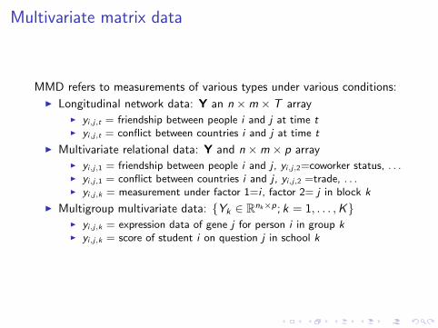
Multivariate matrix data
MMD refers to measurements of various types under various conditions:
I Longitudinal network data: Y an n ×m × T arrayI yi,j,t = friendship between people i and j at time tI yi,j,t = conflict between countries i and j at time t
I Multivariate relational data: Y and n ×m × p arrayI yi,j,1 = friendship between people i and j , yi,j,2=coworker status, . . .I yi,j,1 = conflict between countries i and j , yi,j,2 =trade, . . .I yi,j,k = measurement under factor 1=i , factor 2= j in block k
I Multigroup multivariate data: {Yk ∈ Rnk×p; k = 1, . . . ,K}I yi,j,k = expression data of gene j for person i in group kI yi,j,k = score of student i on question j in school k

Cold War data
Cooperation and conflict data collected on 85 countries every fifth year
1950
AFG
AUL
BUL
CANCHN
DOM
ECU
EGY
FRN
GRC
HAI
HUN
IND
ISRJOR
MYA
NEW
PAK
PER
PHIPRK
ROK RUM
SYR
TAW
TUR
UKGUSA USRYUG
1955
AFG
ALB
ARG
BUL
CHL
CHN
COS
ECUEGY
IND
ISR
ITA
JOR
JPN
MYA
NIC
PAK
PER
POR
PRK
ROK
SAU
SWD
SYR
TAW
THI
TUR
UKGUSA
USR
1960
AFG
ARGAUS BEL
CHL
CHN
CUB
EGY
HUN
ICE
IND
INS IRNIRQISR
ITA
JOR
JPN
NEP
NOR
NTH
PAKPRKROK
TUR
UKG
USAUSR
1965
ARG
AUL
CHL
CHN
EGY
IND
INS
IRNIRQ
ISRJOR
JPN
LEB
NEP
NEW
PAK
PRK
ROK
SAU SPNSYR
TAW
THI
TUR
UKG
USAUSR
1970
AULCHN
EGY
GUA
IND
IRN
IRQ
ISRJOR
NEWPAK
PHI
PRK
ROK
SAL
SYR
THI
UKG
USAUSR
1975
CAN
CHN
CUB
EGY
GRCGUAICE
IND
INS
IRNIRQ
ISRJPNLEB
MYA
POR
PRKROKSAFSYR
THI
TURUKG
USAUSR
1980
AFGARG
CAN
CHL
CHN
COL
CUB
ECU
GFR
IRNIRQ
ISR
ITA
JORLEB
MYA
NIC
NOR
NTH
PAK
PRKROK
SAF
SYR
THI
UKGUSAUSR
YUG
How can we numerically describe variability, similarity across Y1, . . . ,Y7?

Leukemia data
Gene expression data on 327 cancer patients, each in one of seven groups:
group BCR E2A Hyperdip50 MLL T TEL othersample size 15 27 64 20 43 79 79
We look at the 300 genes with highest rank variation across subjects.
●
●
●
●
●
●
●
●
●
●
●
●
●
●
●●
●
●
●
●
●
●
●
●
●
●
●
●
●
●
●
●
●
●
●
●
● ●●
●
●
●
●
●
●
●
●●
●
●
●
●
●
●
●
●
●
●
●
●
●
●
●
●
●
●
●
●
●
● ●
●
●
●
●
●
●
●
●
●
●
●
●
●
●●
●
●
●
● ●
●
●
●
●
●
●●●
●
●
●
●●
●
●
●
●
●
●
●
●
●
●
●
●
●
●
●
●●
●
●
●
●
●
●
●
●
●
●
●
●
●
●
●
●
●
●
●
●
●
●
●
●
●
●
●
●
●
●●
●
●
●
●
●●
●
●
●
●
●
●
●
●●
●●
●
●●
●
●
●
●
●
●
●
●
●
●
●
●
●
●
●
●
●
●
●
●
●
●
●
●
●
●
●
●
●
●
●
●
●
●
●
●
●
●●
●
●
●
●
●
●
●
●
●
●
●●
●
●
●
●
●
●
●
●
●●
●
●
●
●
●
●
●
●
●
●
●
●
●
●
●
●
●
●
●●
●
●
●
●
●
●
●
●
●
●
●
●
●
●
●
●
●
●
●
●
●●
●
●
●
●
●
●●
●
●
●●
●
●
●
●
●
●
●
●
●
●
●
●
●
●
●
●
●
●
●
●
●
●
●
●
●
●
●
●
●
●●
●
●
●
●
●
●
●
●●●
u1
u 3
0 10000 20000 30000 40000
−0.
50.
00.
51.
0
rank of mean correlation
corr
elat
ion
●
●
●
●●
●●
●
●●
●
●
●●
●
●
●
●
●●
●
●
●●●
●●
●●●
●
●
●
●
●●
●●●
●
●
●
●
●
●
●
●
●
●
●●
●
●
●
●
●●●
●
●
●●
●
●
●●●
●●
●●●●●
●
●
●●●●●
●●
●●
●
●
●
●●
●
●●
●
●
●●
●●●
●
●●
●
●
●
●●●
●
●
●
●
●
●
●
●●
●
●
●
●
●
●●
●
●
●
●
●
●
●
●●●●
●
●
●●●
●
●
●
●
●
●
●●
●●●
●●●
●
●●●●
●
●
●
●
●
●
●●
●
●●
●
●●●●
●
●●●●●●
●
●●
●
●●●●●
●
●
●
●
●
●
●
●●
●
●
●
●●
●●
●
●●●
●
●●●
●●
●●
●
●●
●
●
●
●●●
●
●●●
●
●●●
●
●
●
●
●
●
●
●●
●●
●●
●
●
●
●
●
●
●
●●
●
●●
●
●●●●
●●
●●
●
● ●●
●
●
●
●
●
●●
●
●
●●●
●
●●●●
●
●●●
●●
●
●
● ●
●
●
●
●
●
●●
●
●
●●
●
●
●●
●
●
●●
●
●
●●●
●●
● ●●
●
●
●●●●
●●●
●
●
●●
●
●●
●
●●
●
●
●●
●●●
●●●
●●
●
●
●
●
●
●
●
●●●●
●●
●
●
●●
●●
●●
●
● ●
●
●
●
●
●
●
●
●
●●●●
●
●
●●
●
●●
●
●
●
●●●●
●
●●
●
●
●
●
●
●
●●●●●
●
●
●
●
●
●
●●●●
●
●
●●●
●
●
●●
●●
●●
●
●
●●
●●
●
●
●
●
●
●
●
●
●
●
●
●●
●●
●●●
●
●
●●●
●
●
●
●
●●●●
●
●●
●
●●
●
●
●
●
●
●●
●
●
●
●●●
●●
●●
●
●
●
●
●●
●
●●
●
●
●
●●
●
●●●
●
●●●
●
●
●●
●
●
●
●
●
●
●●
●●
●●●
●
●●●
●
●●
●
●
●
●
●
●●
●
●
●
●
●
●●
●
●●●
●
●●●●
●
●
●
●
●
●
●
●
●
●
●
●●
●●
●
●●
●
●●●
●●
●
●
●●
●
●●
●
●
●
●
●●
●
●
●●
●
●●●●●●
●●
●
●●●●
●
●●
●
●●●
●●
●
●●
●
●
●
●
●●
●
●
●
●●●
● ●●
●
●●
●
●
●●●●●●
●
●
●
●
●●●●
●
●
●●●
●
●
●
●●●
●
●
●
●●
●
●
●●
●
●●●
●
●
●
●●
●●●
●●●●
●
●●
●
●●
●
●
●●
●●
●
●●
●
●●
●
●
●
●●●●
●●
●
●●●
●●●
●
●
●●
●●●●
●●
●
●●
●●
●
●
●
●
●
●
●
●
●
●●
●●
●●●●●
●
●
●●
●●●
●
●
●
●●
●
●
●●
●●
●
●
●
●
●
●
●
●
●●
●●
●
●●●●●
●
●
●●●
●●
●
●
●
●●●
●●
●
●
●●
●●
●
●●
●●
●
●●
●
●
●●
●●●
●
●●●
●
●●●
●
●
●●
●
●
●
●●
●
●●●
●
●
●
●
●●
●
●●●
●●●
●
●
●
●●●●●
●●
●●
●●
●●
●●●●●
●●●
●●●
●
●●●
●
●●
●●
●●●
●
●
●
●
●●
●●●
●
●
●
●
●
●
●
●
●●
●
●
●
●●
●●
●●
●●●●
●
●●●
●
●
●
●●
●
●
●●
●
●
●●
●
●
●●
●●
●
●
●●
●
●
●
●
●●
●
●
●●
●
●
●●
●
●
●●●
●
●
● ●
●
●●
●
●
●●
●
●●
●
●
●
●●
●●
●●
●●●●
●●
●
●
●●●●
●
●
●
●
●●
●
●●
●●
●
●
●●●●●●
●
●●
●●
●●●
●
●●
●●
●
●
●●
●
●●●
●
●
●
●
●
●
●
●
●
●
●●
●
●●
●
●●●●●
●
●
●
●●
●●
●
●●●
●●
●●●●
●●
●
●●●
●●●
●
●●
●●
●
●
●
●
●●●
●
●
●
●
●
●
●
●
●●
●
●
●
●
●●
●
●●●
●
●●●●
●
●●●●
●
●
●
●
●●
●
●
●
●●
●●●
●
●●
●●●
●●●●
●●
●
●
●
●●
●
●
●
●
●
●
●
●●●
●●●●●
●
●
●●●●
●
●
●●●
●
●
●
●●●
●
●
●
●
●
●
●
●●
●
●●
●
●
●●
●●●
●
●●●
●
●
●
●
●
●
●
●●●
●
●
●●●
●●
●
●●
●
●
●
●
●
●
●●
●
●
●
●●
●
●
●
●
●●
●
●●
●
●●
●
●
●
●
●
●●●●
●●
●●
●●●
●
●
●●
●●
●●
●
●
●●●
●
●
●
●
●
●
●
●●●
●
●
●
●
●●
●●●●
●
●
●●
●●●●●
●●
●
●●
●
●
●●
●
●●●
●●
●
●
●
●●
●●●
●●
●
●
●
●●
●
●
●●
●●●●●●
●
●●●
●
●●●●
●
●
●●
●●
●
●
●
●
●●
●
●●
●
●
●●
●
●
●
●●
●
●●●●
●
●
●
●●
●
●●
●●
●●●
●
●●
●
●
●
● ●●●●
●
●
●
●
●●
●
●●
●●
●
●
●
●●
●
●
●●
●
●●
●
●●
●
●
●
●● ●
●●
●●
●
●
●●
●
●
●
●● ●
●
●●
●●●●●
●
●
●
●●●
●
●
●●●
●
●
●
●●
●●
●●
●
●●
●
●●
●
●●
●
●●●
●●●
●
●
●
●●●
●
●
●●
●
●
●
●●
●●
●
●
●
●●●●●
Y = UDVT Left-singular vectors of U separate the groups.Yk = UkDkV
Tk How do correlations VkD
2kV
Tk vary across groups?

Reduced rank matrix approximation
Low rank approximations are useful for describing row/column variability:
Symmetric matrices: Y = UΛUT + E , yi,j = uTi Λuj + ei,j
Rectangular matrices: Y = UDVT + E, yi,j = uTi Dvj + ei,j
The column dimension R of U is generally much smaller than that of Y,
R << min(m, n)
so that UΛUT , UDVT provide low-rank approximations to Y.
minM:rank(M)=R
||Y−M||2 = ||Y− U[,1:R]D[1:R,1:R]VT
[,1:R]||2
●
●
●●
●●●●●●●●●●●●●●●●●●●●●●●●●●●●●●●●●●●●●●●●●●●●●●●●●●●●●●●●●●●●●●●●●●●●●●●●●●●●●●●●●●●●●●●●●●●●●●●●●●●●●●●●●●●●●●●●●●●●●●●●●●●●●●●●●●●●●●●●●●●●●●●●●●●●●●●●●●●●●●●●●●●●●●●●●●●●●●●●●●●●●●●●●●●●●●●●●●●●●●●●●●●●●●●●●●●●●●●●●●●●●●●●●●●●●●●●●●●●●●●●●●●●●●●●●●●●●●●●●●●●●●●●●●●●●●●●●●●●●●●●●●●●●●●●●●●●●●●●
0 50 150 250
020
4060
80si
ngul
ar v
alue
s
−4 −2 0 2 4
−4
−2
02
4
y
y
R=3
−4 −2 0 2 4
−4
−2
02
4
y
y
R=9
−4 −2 0 2 4
−4
−2
02
4
y
y
R=27
−4 −2 0 2 4
−4
−2
02
4
y
y
R=81

Model-based estimation
Ym×n = UDVT + E
I U and V are m × R and n × R orthonormal matrices ;
I D is a diagonal matrix of positive numbers;
I E is a matrix of i.i.d. Gaussian noise.
Parameters to estimate include U,D,V and the error variance. Why notjust use the SVD?
I Estimation: MSE of LS estimate can be very high.
I Missing data and prediction.
I A model accommodates regression, non-normal and hierarchicaldata.

Pooling information
Consider p variables measured on individuals in K groups, and let Y bethe nk × p data matrix for group k.
Y1 = U1D1VT1 + E1
......
...
YK = UKDKVTK + EK
Recall, E [YTk Y] = VkD
2kV
Tk , so Vk represents the covariance/principle
components of the observations in group k. Should we
I assume V1 = V2 = · · · = VK ?
I estimate each Vk separately (perhaps using SVD)?
I do something in-between?
Vk = wkVk + (1− wk)∑j 6=k
θkVj
A model for heterogeneity among {V1, . . . ,VK} would help determinethe right balance.
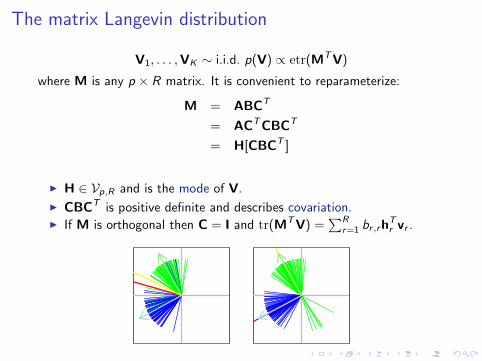
The matrix Langevin distribution
V1, . . . ,VK ∼ i.i.d. p(V) ∝ etr(MTV)
where M is any p × R matrix. It is convenient to reparameterize:
M = ABCT
= ACTCBCT
= H[CBCT ]
I H ∈ Vp,R and is the mode of V.
I CBCT is positive definite and describes covariation.I If M is orthogonal then C = I and tr(MTV) =
∑Rr=1 br ,rh
Tr vr .

A hierarchical eigenmodel
Y1 = U1D1VT1 + E1
......
...
YK = UKDKVTK + EK
U1 ∼ uniform(Vn1,R) diag(D1) ∼ normal(0, τ 2I ) V1 ∼ Langevin(M)
...
UK ∼ uniform(VnK ,R) diag(DK ) ∼ normal(0, τ 2I ) VK ∼ Langevin(M)
M = ABCT
A ∼ uniform(Vp,R)
diag(B) ∼ normal+(0, η2I )
C ∼ uniform(VR,R)

Full conditional distributions
p(V1, . . . ,VK |A,B,CT ) =K∏
k=1
c(B)etr(CBATVk)
= c(B)Ketr(KCBAT V)
Evidently,
p(A|V1, . . . ,VK ,B,C) ∝ etr([K VCB]TA)
p(C|V1, . . . ,VK ,A,B) ∝ etr([K VTAB]TC)
Additionally,
I The full conditional of B is nonstandard but low-dimensional.
I The full conditional distributions of {Uk} and {Vk} are Langevin.
I Full conditional distributions of {Dk , σk} are standard.
Gibbs sampling can be implemented with the aid of a rejection samplerfor the matrix Langevin distribution.

Leukemia data analysis
group BCR E2A Hyperdip50 MLL T TEL other
sample size 15 27 64 20 43 79 79
●
●
●
●
●
●
●
●
●
●
●
●
●
●
●●
●
●
●
●
●
●
●
●
●
●
●
●
●
●
●
●
●
●
●
●
● ●●
●
●
●
●
●
●
●
●●
●
●
●
●
●
●
●
●
●
●
●
●
●
●
●
●
●
●
●
●
●
● ●
●
●
●
●
●
●
●
●
●
●
●
●
●
●●
●
●
●
● ●
●
●
●
●
●
●●●
●
●
●
●●
●
●
●
●
●
●
●
●
●
●
●
●
●
●
●
●●
●
●
●
●
●
●
●
●
●
●
●
●
●
●
●
●
●
●
●
●
●
●
●
●
●
●
●
●
●
●●
●
●
●
●
●●
●
●
●
●
●
●
●
●●
●●
●
●●
●
●
●
●
●
●
●
●
●
●
●
●
●
●
●
●
●
●
●
●
●
●
●
●
●
●
●
●
●
●
●
●
●
●
●
●
●
●●
●
●
●
●
●
●
●
●
●
●
●●
●
●
●
●
●
●
●
●
●●
●
●
●
●
●
●
●
●
●
●
●
●
●
●
●
●
●
●
●●
●
●
●
●
●
●
●
●
●
●
●
●
●
●
●
●
●
●
●
●
●●
●
●
●
●
●
●●
●
●
●●
●
●
●
●
●
●
●
●
●
●
●
●
●
●
●
●
●
●
●
●
●
●
●
●
●
●
●
●
●
●●
●
●
●
●
●
●
●
●●●
u1
u 3
0 10000 20000 30000 40000
−0.
50.
00.
51.
0
rank of mean correlation
corr
elat
ion
●
●
●
●●
●●
●
●●
●
●
●●
●
●
●
●
●●
●
●
●●●
●●
●●●
●
●
●
●
●●
●●●
●
●
●
●
●
●
●
●
●
●
●●
●
●
●
●
●●●
●
●
●●
●
●
●●●
●●
●●●●●
●
●
●●●●●
●●
●●
●
●
●
●●
●
●●
●
●
●●
●●●
●
●●
●
●
●
●●●
●
●
●
●
●
●
●
●●
●
●
●
●
●
●●
●
●
●
●
●
●
●
●●●●
●
●
●●●
●
●
●
●
●
●
●●
●●●
●●●
●
●●●●
●
●
●
●
●
●
●●
●
●●
●
●●●●
●
●●●●●●
●
●●
●
●●●●●
●
●
●
●
●
●
●
●●
●
●
●
●●
●●
●
●●●
●
●●●
●●
●●
●
●●
●
●
●
●●●
●
●●●
●
●●●
●
●
●
●
●
●
●
●●
●●
●●
●
●
●
●
●
●
●
●●
●
●●
●
●●●●
●●
●●
●
● ●●
●
●
●
●
●
●●
●
●
●●●
●
●●●●
●
●●●
●●
●
●
● ●
●
●
●
●
●
●●
●
●
●●
●
●
●●
●
●
●●
●
●
●●●
●●
● ●●
●
●
●●●●
●●●
●
●
●●
●
●●
●
●●
●
●
●●
●●●
●●●
●●
●
●
●
●
●
●
●
●●●●
●●
●
●
●●
●●
●●
●
● ●
●
●
●
●
●
●
●
●
●●●●
●
●
●●
●
●●
●
●
●
●●●●
●
●●
●
●
●
●
●
●
●●●●●
●
●
●
●
●
●
●●●●
●
●
●●●
●
●
●●
●●
●●
●
●
●●
●●
●
●
●
●
●
●
●
●
●
●
●
●●
●●
●●●
●
●
●●●
●
●
●
●
●●●●
●
●●
●
●●
●
●
●
●
●
●●
●
●
●
●●●
●●
●●
●
●
●
●
●●
●
●●
●
●
●
●●
●
●●●
●
●●●
●
●
●●
●
●
●
●
●
●
●●
●●
●●●
●
●●●
●
●●
●
●
●
●
●
●●
●
●
●
●
●
●●
●
●●●
●
●●●●
●
●
●
●
●
●
●
●
●
●
●
●●
●●
●
●●
●
●●●
●●
●
●
●●
●
●●
●
●
●
●
●●
●
●
●●
●
●●●●●●
●●
●
●●●●
●
●●
●
●●●
●●
●
●●
●
●
●
●
●●
●
●
●
●●●
● ●●
●
●●
●
●
●●●●●●
●
●
●
●
●●●●
●
●
●●●
●
●
●
●●●
●
●
●
●●
●
●
●●
●
●●●
●
●
●
●●
●●●
●●●●
●
●●
●
●●
●
●
●●
●●
●
●●
●
●●
●
●
●
●●●●
●●
●
●●●
●●●
●
●
●●
●●●●
●●
●
●●
●●
●
●
●
●
●
●
●
●
●
●●
●●
●●●●●
●
●
●●
●●●
●
●
●
●●
●
●
●●
●●
●
●
●
●
●
●
●
●
●●
●●
●
●●●●●
●
●
●●●
●●
●
●
●
●●●
●●
●
●
●●
●●
●
●●
●●
●
●●
●
●
●●
●●●
●
●●●
●
●●●
●
●
●●
●
●
●
●●
●
●●●
●
●
●
●
●●
●
●●●
●●●
●
●
●
●●●●●
●●
●●
●●
●●
●●●●●
●●●
●●●
●
●●●
●
●●
●●
●●●
●
●
●
●
●●
●●●
●
●
●
●
●
●
●
●
●●
●
●
●
●●
●●
●●
●●●●
●
●●●
●
●
●
●●
●
●
●●
●
●
●●
●
●
●●
●●
●
●
●●
●
●
●
●
●●
●
●
●●
●
●
●●
●
●
●●●
●
●
● ●
●
●●
●
●
●●
●
●●
●
●
●
●●
●●
●●
●●●●
●●
●
●
●●●●
●
●
●
●
●●
●
●●
●●
●
●
●●●●●●
●
●●
●●
●●●
●
●●
●●
●
●
●●
●
●●●
●
●
●
●
●
●
●
●
●
●
●●
●
●●
●
●●●●●
●
●
●
●●
●●
●
●●●
●●
●●●●
●●
●
●●●
●●●
●
●●
●●
●
●
●
●
●●●
●
●
●
●
●
●
●
●
●●
●
●
●
●
●●
●
●●●
●
●●●●
●
●●●●
●
●
●
●
●●
●
●
●
●●
●●●
●
●●
●●●
●●●●
●●
●
●
●
●●
●
●
●
●
●
●
●
●●●
●●●●●
●
●
●●●●
●
●
●●●
●
●
●
●●●
●
●
●
●
●
●
●
●●
●
●●
●
●
●●
●●●
●
●●●
●
●
●
●
●
●
●
●●●
●
●
●●●
●●
●
●●
●
●
●
●
●
●
●●
●
●
●
●●
●
●
●
●
●●
●
●●
●
●●
●
●
●
●
●
●●●●
●●
●●
●●●
●
●
●●
●●
●●
●
●
●●●
●
●
●
●
●
●
●
●●●
●
●
●
●
●●
●●●●
●
●
●●
●●●●●
●●
●
●●
●
●
●●
●
●●●
●●
●
●
●
●●
●●●
●●
●
●
●
●●
●
●
●●
●●●●●●
●
●●●
●
●●●●
●
●
●●
●●
●
●
●
●
●●
●
●●
●
●
●●
●
●
●
●●
●
●●●●
●
●
●
●●
●
●●
●●
●●●
●
●●
●
●
●
● ●●●●
●
●
●
●
●●
●
●●
●●
●
●
●
●●
●
●
●●
●
●●
●
●●
●
●
●
●● ●
●●
●●
●
●
●●
●
●
●
●● ●
●
●●
●●●●●
●
●
●
●●●
●
●
●●●
●
●
●
●●
●●
●●
●
●●
●
●●
●
●●
●
●●●
●●●
●
●
●
●●●
●
●
●●
●
●
●
●●
●●
●
●
●
●●●●●
Data Y is 327× 300, orcan be broken into{Y1, . . . ,Y7} of variablerow dimension butcommon columndimension.
We’ll fit the hierarchical eigenmodel and evaluate its goodness-of-fitusing the matrix similarity statistic
t(Y1, . . . ,Y7) =∑i<j
tr(|ATi Aj |),
where Ak is Yk with the “subject effects removed:”
Yk = UDVT
Ak = DVT

Goodness of fit
700 800 900 1000 1100
0.00
00.
005
0.01
00.
015
700 800 900 1000 1100
0.00
00.
005
0.01
00.
015
posterior predictive matrix similarity700 800 900 1000 1100
0.00
00.
005
0.01
00.
015 no pooling
complete poolingmodel−based poolingobserved value

International relations data
Ordered probit model for discrete data:
yi,j,k =∑
x∈{−1,0,+1}
xδIx (zi,j.k)
Eigenvalue decomposition model for latent Z:
Zk = UkΛkUTk + Ek
U1, . . . ,UK ∼ i.i.d. Langevin(M)
Λ1, . . . ,ΛK ∼ i.i.d. mvn(0, τ 2I)
Parameter estimation is similar to before: Letting M = ABCT ,
p(A|U1, . . . ,UK ,B,C) ∝ etr([K UCB]TA)
p(C|U1, . . . ,UK ,A,B) ∝ etr([K UTAB]TC), although
p(Uk |Zk ,M) ∝ etr(MTUk + UkZkUTk )
This last distribution is a Bingham-Langevin distribution.

International relations data
●
●● ●
●
●
●
1950 1960 1970 1980
−50
50
● ●
●
●●
●
●
1950 1960 1970 1980
−50
50
● ● ● ●●
●
●
1950 1960 1970 1980
−50
50
0 20 40 60 80
−20
2060
AFGALB
ANDARG
AUL
AUS
BELBHUBOL
BRABUL
CANCHL
CHN
COL
COSCUB
CZEDEN
DOMECUEGY
ETHFIN
FRNGDR
GFRGRCGUA
HAIHON
HUNICE
INDINSIRE
IRNIRQ
ISRITAJOR
JPNLBRLEB
LIELUX
MEX
MNC
MONM
YA
NEP
NEW
NIC
NORNTHOMA
PAKPANPARPER
PHIPOL
POR
PRK
ROK
RUMSAF
SALSAU
SNMSPN
SRISW
DSW
ZSYR
TAW
THITURUKG
URU
USA
USR
VEN
YEMYUG
0 20 40 60 80
−10
05
10
AFGALBANDARG
AULAUS
BELBHU
BOLBRA
BULCAN
CHLCHN
COLCOS
CUBCZE
DENDOM
ECU
EGYETH
FINFRNGDR
GFRGRCGUA
HAI
HON
HUNICE
INDINSIRE
IRN
IRQ
ISR
ITAJORJPN
LBR
LEBLIELUXM
EX
MNC
MONM
YANEP
NEWNICNORNTH
OMAPAK
PANPARPER
PHIPOL
PORPRK
ROKRUM
SAF
SALSAUSNM
SPNSRISWD
SWZ
SYRTAWTHI
TURUKG
URUUSA
USR
VEN
YEMYUG
0 20 40 60 80
−10
05
AFG
ALBAND
ARG
AULAUS
BELBHUBOL
BRABULCAN
CHL
CHN
COLCOSCUB
CZEDEN
DOM
ECU
EGY
ETHFINFRN
GDRGFR
GRC
GUAHAIHON
HUN
ICE
IND
INSIREIRN
IRQ
ISR
ITA
JOR
JPN
LBR
LEBLIE
LUXM
EXM
NCM
ONMYANEP
NEW
NICNOR
NTHOM
A
PAK
PANPAR
PER
PHIPOLPOR
PRKROK
RUMSAFSAL
SAUSNMSPNSRI
SWD
SWZ
SYR
TAW
THI
TURUKGURU
USAUSR
VENYEMYUG
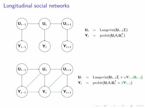
Longitudinal social networks
Ut−1 Ut Ut+1
Yt−1 Yt Yt+1
Ut−1 Ut Ut+1
Yt−1 Yt Yt+1
Ut ∼ Langevin(Ut−1Σ)
Yt ∼ probit(UtΛtUTt )
Ut ∼ Langevin(Ut−1Σ + αYt−1Ut−1)
Yt ∼ probit(UtΛtUTt + βYt−1)

A simulated network

Another simulated network

Discussion
Summary:
I SVD and EVD are natural ways to describe matrix patterns.
I Variability across matrices can be described by variability acrossdecompositions.
I Modeling variability allows for information sharing across datasets.
I Parameter estimation can be done with Gibbs sampling.
Caveats:
I Interpretation of parameters is subtle.
I Models are more “statistical” than “generative.”


