
Heart of Missouri United Way Community Development Training Series
Module III: Data Management & Analysis Aaron M. Thompson
School of Social Work
University of Missouri
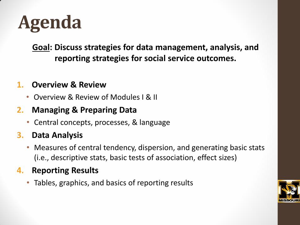
Agenda Goal: Discuss strategies for data management, analysis, and
reporting strategies for social service outcomes.
1. Overview & Review
• Overview & Review of Modules I & II
2. Managing & Preparing Data
• Central concepts, processes, & language
3. Data Analysis
• Measures of central tendency, dispersion, and generating basic stats (i.e., descriptive stats, basic tests of association, effect sizes)
4. Reporting Results
• Tables, graphics, and basics of reporting results
OVERVIEW & REVIEW
Overview & Review of Modules I & II
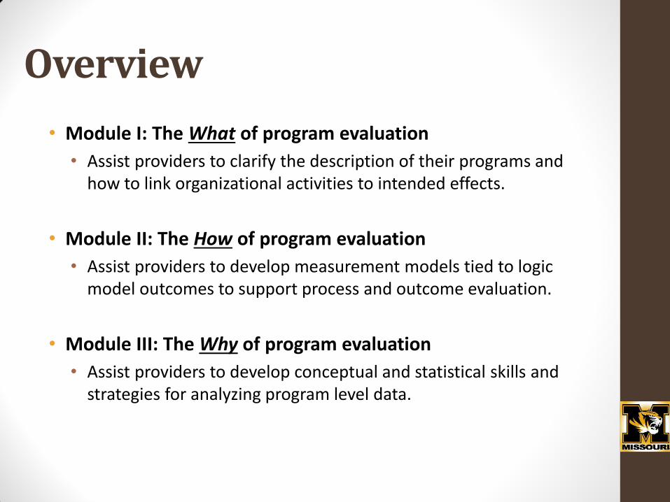
Overview
• Module I: The What of program evaluation
• Assist providers to clarify the description of their programs and how to link organizational activities to intended effects.
• Module II: The How of program evaluation
• Assist providers to develop measurement models tied to logic model outcomes to support process and outcome evaluation.
• Module III: The Why of program evaluation
• Assist providers to develop conceptual and statistical skills and strategies for analyzing program level data.
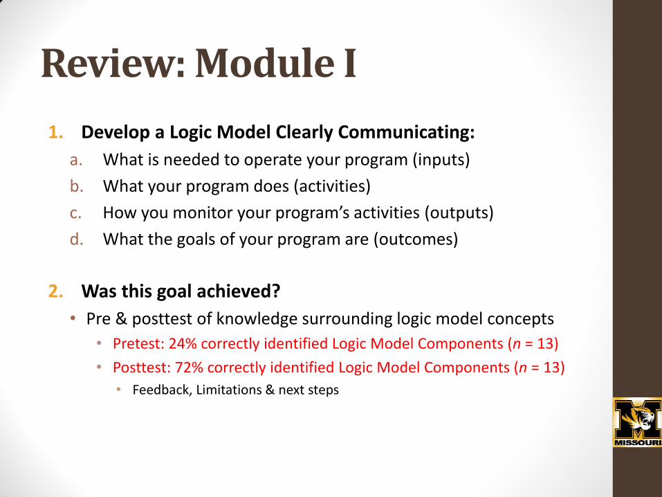
Review: Module I
1. Develop a Logic Model Clearly Communicating:
a. What is needed to operate your program (inputs)
b. What your program does (activities)
c. How you monitor your program’s activities (outputs)
d. What the goals of your program are (outcomes)
2. Was this goal achieved?
• Pre & posttest of knowledge surrounding logic model concepts
• Pretest: 24% correctly identified Logic Model Components (n = 13)
• Posttest: 72% correctly identified Logic Model Components (n = 13)
• Feedback, Limitations & next steps
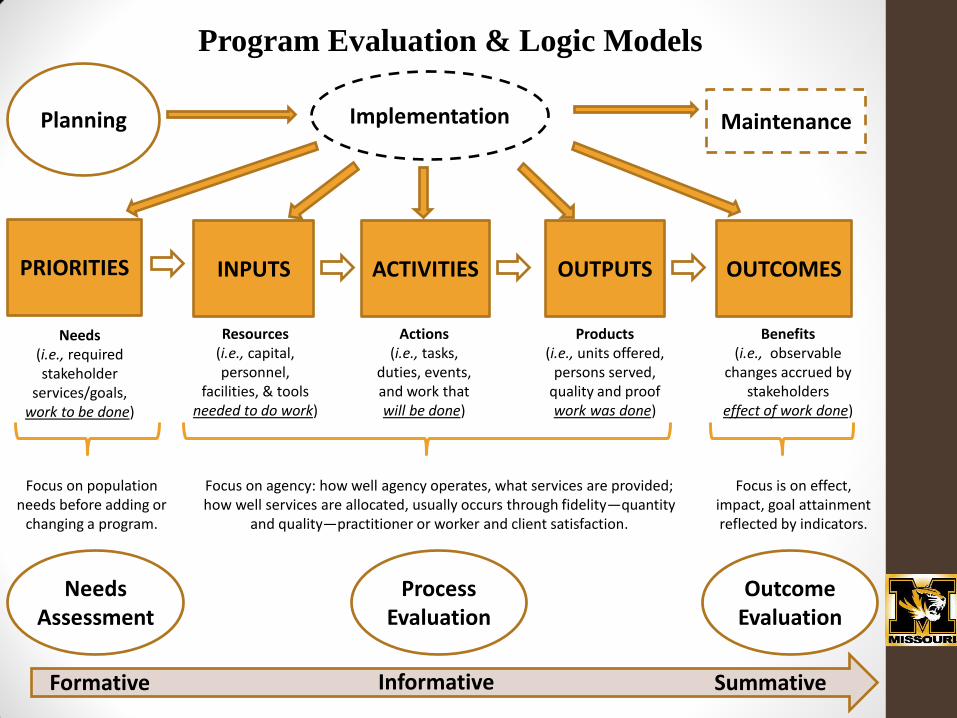
INPUTS ACTIVITIES OUTPUTS OUTCOMES
Resources (i.e., capital, personnel,
facilities, & tools needed to do work)
Actions (i.e., tasks,
duties, events, and work that will be done)
Products (i.e., units offered,
persons served, quality and proof work was done)
Benefits (i.e., observable
changes accrued by stakeholders
effect of work done)
Planning Implementation
Process Evaluation
Outcome Evaluation
Program Evaluation & Logic Models
Focus on population needs before adding or
changing a program.
Summative Formative
Focus on agency: how well agency operates, what services are provided; how well services are allocated, usually occurs through fidelity—quantity
and quality—practitioner or worker and client satisfaction.
Focus is on effect, impact, goal attainment reflected by indicators.
Maintenance
Needs (i.e., required stakeholder
services/goals, work to be done)
PRIORITIES
Needs Assessment
Informative

Outcomes & Development • Measureable Benefits for participants after tx exposure
• Links between inputs, activities, and outputs
• HMUW LM follows a sequential developmental progression
Short-term Proximal
Immediate
Interim Medial
Intermediate
Long-term Distal
Impact
Initial changes most causally associated
with program targets
• Knowledge • Attitudes • Cognitions
Secondary changes reasonably expected
to stem from proximal effects
• Skills • Behaviors • Social Interactions
Terminal changes logically expected,
generally reflect goals of agency
• Health • Status • Condition
0-1 years 2-3 years 4-7 years
OUTCOMES
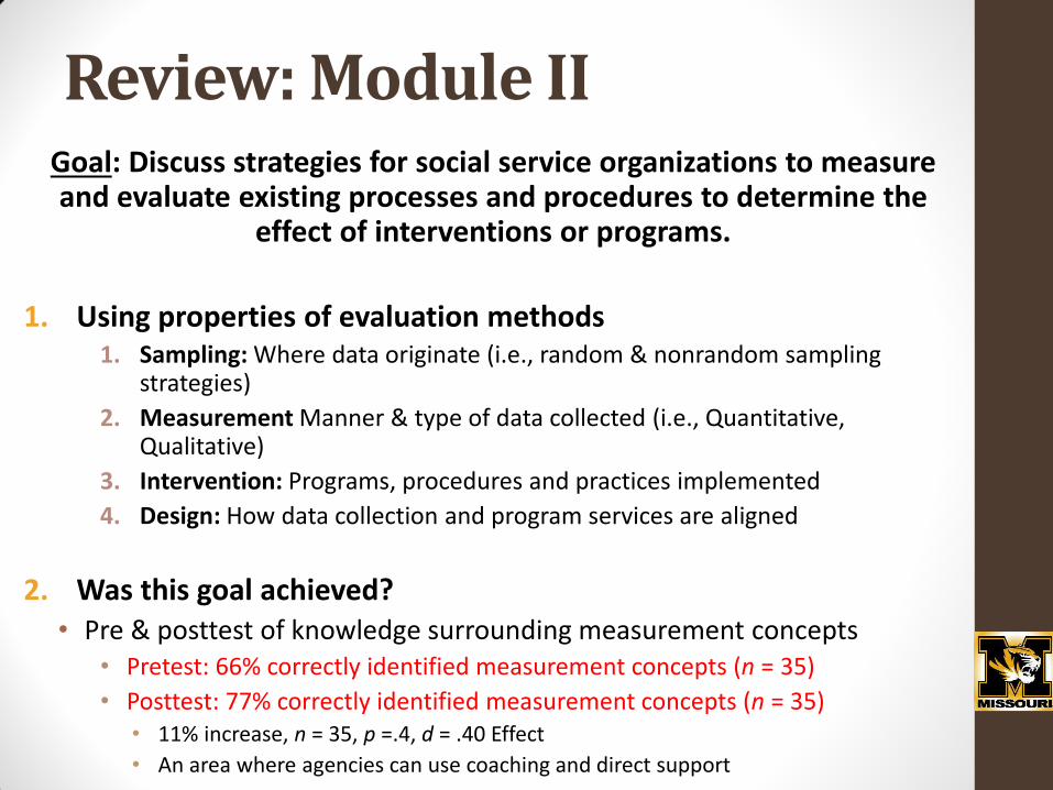
Review: Module II Goal: Discuss strategies for social service organizations to measure and evaluate existing processes and procedures to determine the
effect of interventions or programs.
1. Using properties of evaluation methods 1. Sampling: Where data originate (i.e., random & nonrandom sampling
strategies)
2. Measurement Manner & type of data collected (i.e., Quantitative, Qualitative)
3. Intervention: Programs, procedures and practices implemented
4. Design: How data collection and program services are aligned
2. Was this goal achieved? • Pre & posttest of knowledge surrounding measurement concepts
• Pretest: 66% correctly identified measurement concepts (n = 35)
• Posttest: 77% correctly identified measurement concepts (n = 35) • 11% increase, n = 35, p =.4, d = .40 Effect
• An area where agencies can use coaching and direct support
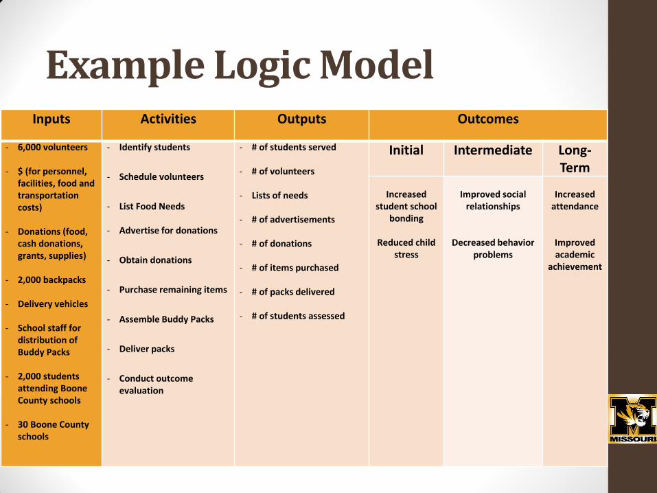
Example Logic Model Inputs Activities Outputs Outcomes
- 6,000 volunteers
- $ (for personnel, facilities, food and transportation costs)
- Donations (food, cash donations, grants, supplies)
- 2,000 backpacks
- Delivery vehicles
- School staff for
distribution of Buddy Packs
- 2,000 students attending Boone County schools
- 30 Boone County schools
- Identify students
- Schedule volunteers
- List Food Needs
- Advertise for donations
- Obtain donations
- Purchase remaining items
- Assemble Buddy Packs
- Deliver packs
- Conduct outcome
evaluation
- # of students served
- # of volunteers
- Lists of needs
- # of advertisements
- # of donations
- # of items purchased
- # of packs delivered
- # of students assessed
Initial
Intermediate Long-Term
Increased
student school bonding
Reduced child
stress
Improved social
relationships
Decreased behavior
problems
Increased
attendance
Improved academic
achievement
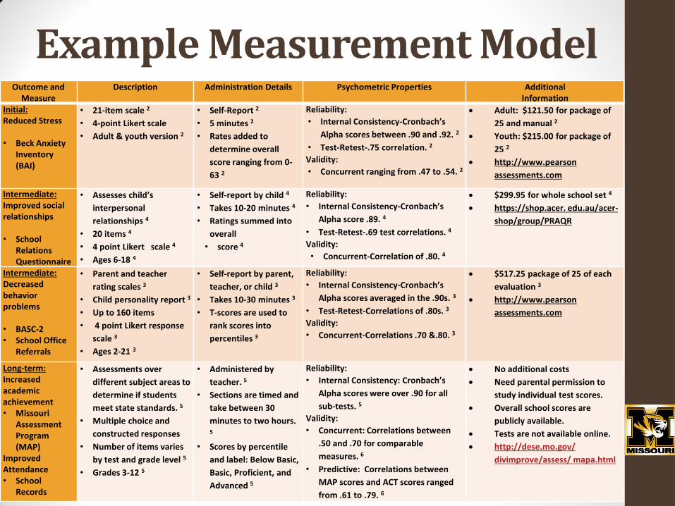
Example Measurement Model
•
Outcome and Measure
Description Administration Details Psychometric Properties Additional Information
Initial: Reduced Stress • Beck Anxiety
Inventory (BAI)
• 21-item scale 2
• 4-point Likert scale
• Adult & youth version 2
• Self-Report 2
• 5 minutes 2
• Rates added to
determine overall
score ranging from 0-
63 2
Reliability:
• Internal Consistency-Cronbach’s
Alpha scores between .90 and .92. 2
• Test-Retest-.75 correlation. 2
Validity:
• Concurrent ranging from .47 to .54. 2
Adult: $121.50 for package of
25 and manual 2
Youth: $215.00 for package of
25 2
http://www.pearson
assessments.com
Intermediate: Improved social relationships • School
Relations Questionnaire
• Assesses child’s
interpersonal
relationships 4
• 20 items 4
• 4 point Likert scale 4
• Ages 6-18 4
• Self-report by child 4
• Takes 10-20 minutes 4
• Ratings summed into
overall
• score 4
Reliability:
• Internal Consistency-Cronbach’s
Alpha score .89. 4
• Test-Retest-.69 test correlations. 4
Validity:
• Concurrent-Correlation of .80. 4
$299.95 for whole school set 4
https://shop.acer. edu.au/acer-
shop/group/PRAQR
Intermediate: Decreased behavior problems • BASC-2 • School Office
Referrals
• Parent and teacher
rating scales 3
• Child personality report 3
• Up to 160 items
• 4 point Likert response
scale 3
• Ages 2-21 3
• Self-report by parent,
teacher, or child 3
• Takes 10-30 minutes 3
• T-scores are used to
rank scores into
percentiles 3
Reliability:
• Internal Consistency-Cronbach’s
Alpha scores averaged in the .90s. 3
• Test-Retest-Correlations of .80s. 3
Validity:
• Concurrent-Correlations .70 &.80. 3
$517.25 package of 25 of each
evaluation 3
http://www.pearson
assessments.com
Long-term: Increased academic achievement • Missouri
Assessment Program (MAP)
Improved Attendance • School
Records
• Assessments over
different subject areas to
determine if students
meet state standards. 5
• Multiple choice and
constructed responses
• Number of items varies
by test and grade level 5
• Grades 3-12 5
• Administered by
teacher. 5
• Sections are timed and
take between 30
minutes to two hours. 5
• Scores by percentile
and label: Below Basic,
Basic, Proficient, and
Advanced 5
Reliability:
• Internal Consistency: Cronbach’s
Alpha scores were over .90 for all
sub-tests. 5
Validity:
• Concurrent: Correlations between
.50 and .70 for comparable
measures. 6
• Predictive: Correlations between
MAP scores and ACT scores ranged
from .61 to .79. 6
No additional costs
Need parental permission to
study individual test scores.
Overall school scores are
publicly available.
Tests are not available online.
http://dese.mo.gov/
divimprove/assess/ mapa.html
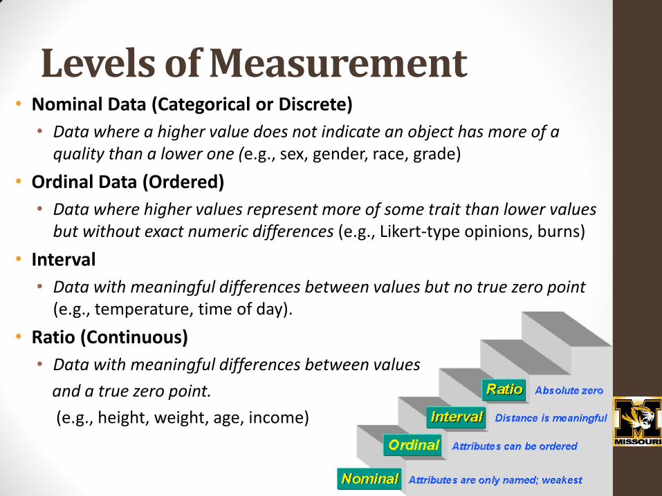
Levels of Measurement • Nominal Data (Categorical or Discrete)
• Data where a higher value does not indicate an object has more of a quality than a lower one (e.g., sex, gender, race, grade)
• Ordinal Data (Ordered)
• Data where higher values represent more of some trait than lower values but without exact numeric differences (e.g., Likert-type opinions, burns)
• Interval
• Data with meaningful differences between values but no true zero point (e.g., temperature, time of day).
• Ratio (Continuous)
• Data with meaningful differences between values
and a true zero point.
(e.g., height, weight, age, income)
DATA MANAGEMENT: DATA ENTRY & PREPARATION
Central Concepts, Processes & Language
Data Management • Data Coding & Entry
• Preparing data: Codebooks & processes
• Checking Data
• Avoiding errors and examining properties
• Data Storage
• Efficiency and process
• Considerations
• Ownership, privacy, and sharing
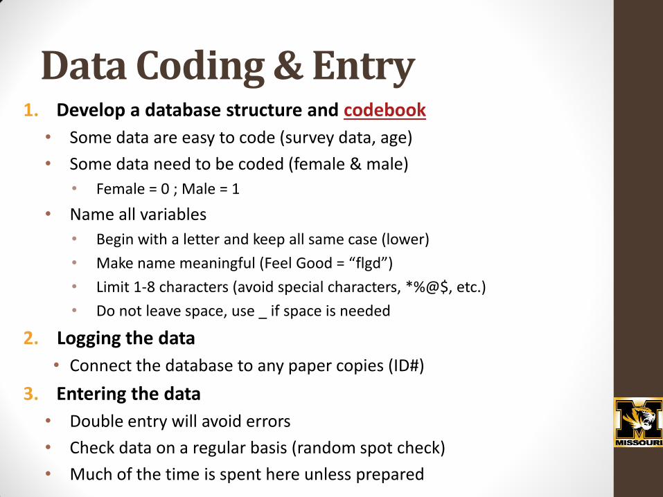
Data Coding & Entry 1. Develop a database structure and codebook
• Some data are easy to code (survey data, age)
• Some data need to be coded (female & male)
• Female = 0 ; Male = 1
• Name all variables
• Begin with a letter and keep all same case (lower)
• Make name meaningful (Feel Good = “flgd”)
• Limit 1-8 characters (avoid special characters, *%@$, etc.)
• Do not leave space, use _ if space is needed
2. Logging the data
• Connect the database to any paper copies (ID#)
3. Entering the data
• Double entry will avoid errors
• Check data on a regular basis (random spot check)
• Much of the time is spent here unless prepared
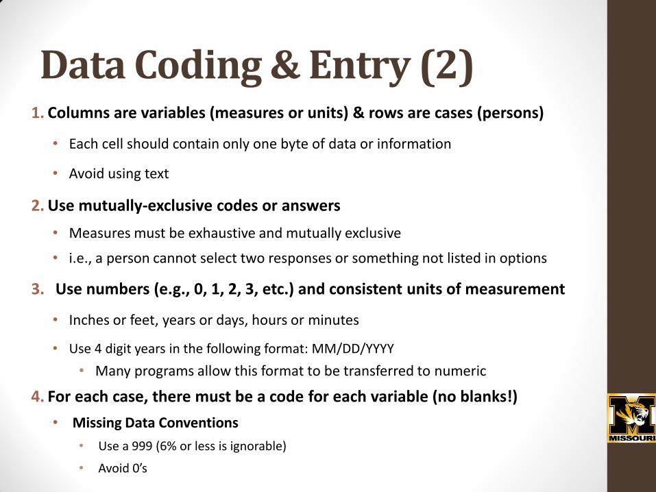
Data Coding & Entry (2) 1. Columns are variables (measures or units) & rows are cases (persons)
• Each cell should contain only one byte of data or information
• Avoid using text
2. Use mutually-exclusive codes or answers
• Measures must be exhaustive and mutually exclusive
• i.e., a person cannot select two responses or something not listed in options
3. Use numbers (e.g., 0, 1, 2, 3, etc.) and consistent units of measurement
• Inches or feet, years or days, hours or minutes
• Use 4 digit years in the following format: MM/DD/YYYY
• Many programs allow this format to be transferred to numeric
4. For each case, there must be a code for each variable (no blanks!)
• Missing Data Conventions
• Use a 999 (6% or less is ignorable)
• Avoid 0’s
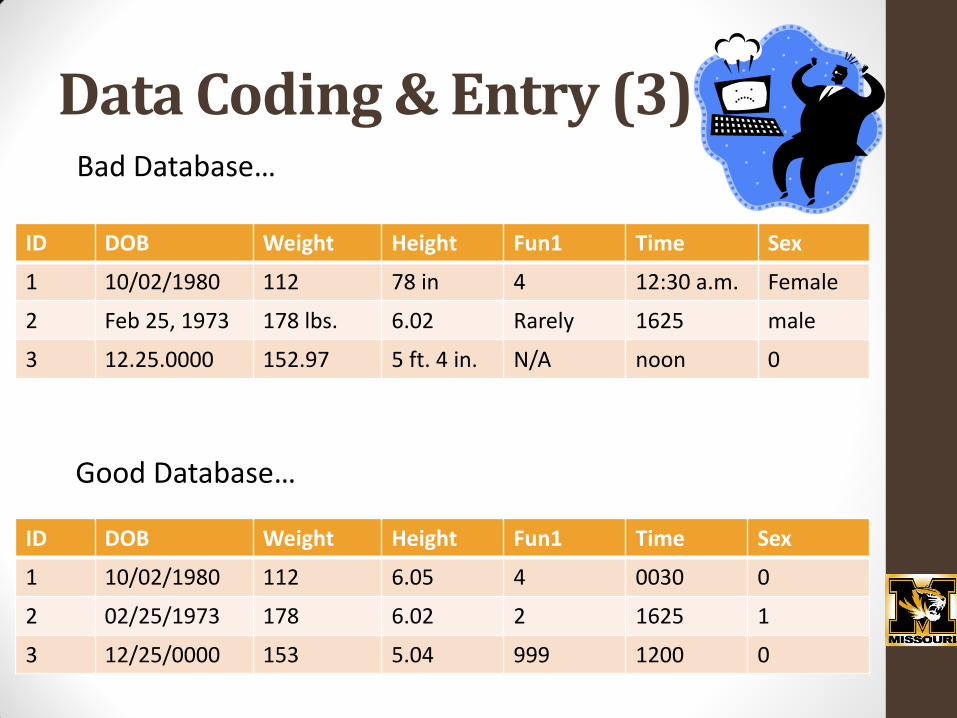
Data Coding & Entry (3) Bad Database…
Good Database…
ID DOB Weight Height Fun1 Time Sex
1 10/02/1980 112 78 in 4 12:30 a.m. Female
2 Feb 25, 1973 178 lbs. 6.02 Rarely 1625 male
3 12.25.0000 152.97 5 ft. 4 in. N/A noon 0
ID DOB Weight Height Fun1 Time Sex
1 10/02/1980 112 6.05 4 0030 0
2 02/25/1973 178 6.02 2 1625 1
3 12/25/0000 153 5.04 999 1200 0
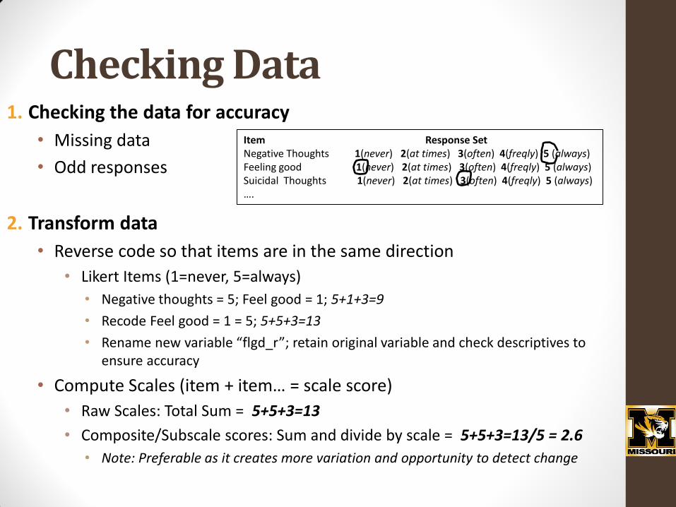
Checking Data 1. Checking the data for accuracy
• Missing data
• Odd responses
2. Transform data
• Reverse code so that items are in the same direction
• Likert Items (1=never, 5=always)
• Negative thoughts = 5; Feel good = 1; 5+1+3=9
• Recode Feel good = 1 = 5; 5+5+3=13
• Rename new variable “flgd_r”; retain original variable and check descriptives to ensure accuracy
• Compute Scales (item + item… = scale score)
• Raw Scales: Total Sum = 5+5+3=13
• Composite/Subscale scores: Sum and divide by scale = 5+5+3=13/5 = 2.6
• Note: Preferable as it creates more variation and opportunity to detect change
Item Response Set Negative Thoughts 1(never) 2(at times) 3(often) 4(freqly) 5 (always) Feeling good 1(never) 2(at times) 3(often) 4(freqly) 5 (always) Suicidal Thoughts 1(never) 2(at times) 3(often) 4(freqly) 5 (always) ….
Considerations • Data Ownership
• Client Rights • Obtaining informed consent • Agency owns data, but consent is required to share data
• Data Retention • Retain enough data so evaluations can be replicated • May not need raw data—but only scales
• Storage & Security • Use of Ids (unique) • Crosswalk files with names and personal data (limited access)
• Links names to ID numbers that are in the larger dataset
• !!! Backup Data in Multiple Formats on a Regular Basis!!! • Create a schedule (every Friday afternoon) • Use Multiple Modes of Backup
• Email copy to self and one other person • Burn copy to a disc or external drive • Back up using Google Docs
• Create a database and directly enter data • School behavioral data • LOVE INC Database
DATA ANALYSIS: ANSWERING THE QUESTION
Qualitative & Quantitative Approaches
Qualitative Analysis
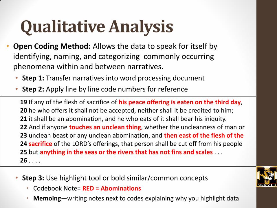
• Open Coding Method: Allows the data to speak for itself by identifying, naming, and categorizing commonly occurring phenomena within and between narratives.
• Step 1: Transfer narratives into word processing document
• Step 2: Apply line by line code numbers for reference
• Step 3: Use highlight tool or bold similar/common concepts
• Codebook Note= RED = Abominations
• Memoing—writing notes next to codes explaining why you highlight data
19 If any of the flesh of sacrifice of his peace offering is eaten on the third day, 20 he who offers it shall not be accepted, neither shall it be credited to him; 21 it shall be an abomination, and he who eats of it shall bear his iniquity. 22 And if anyone touches an unclean thing, whether the uncleanness of man or 23 unclean beast or any unclean abomination, and then east of the flesh of the 24 sacrifice of the LORD’s offerings, that person shall be cut off from his people 25 but anything in the seas or the rivers that has not fins and scales . . . 26 . . . .
Qualitative Analysis (2)
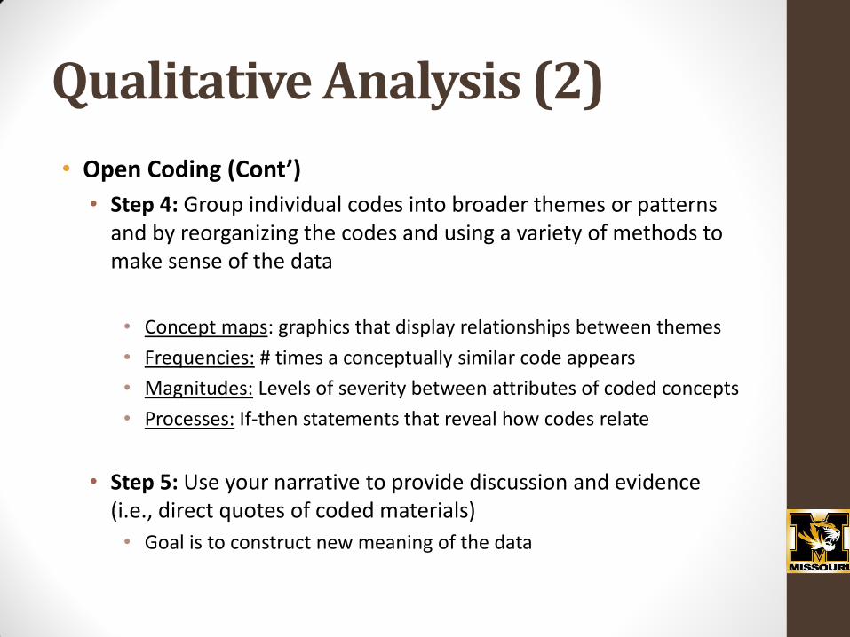
• Open Coding (Cont’)
• Step 4: Group individual codes into broader themes or patterns and by reorganizing the codes and using a variety of methods to make sense of the data
• Concept maps: graphics that display relationships between themes
• Frequencies: # times a conceptually similar code appears
• Magnitudes: Levels of severity between attributes of coded concepts
• Processes: If-then statements that reveal how codes relate
• Step 5: Use your narrative to provide discussion and evidence (i.e., direct quotes of coded materials)
• Goal is to construct new meaning of the data
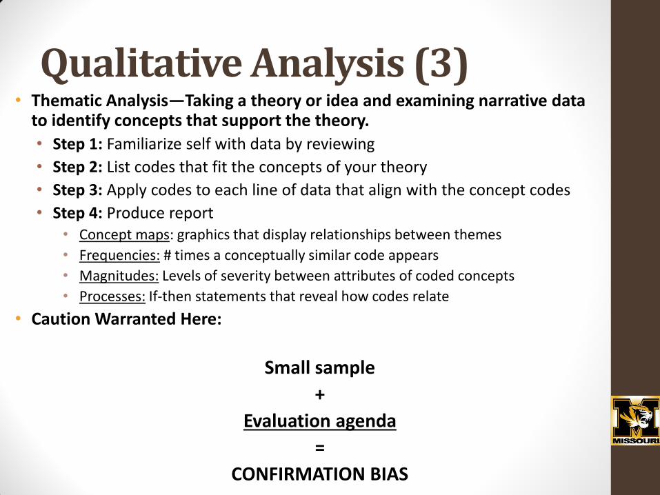
Qualitative Analysis (3) • Thematic Analysis—Taking a theory or idea and examining narrative data
to identify concepts that support the theory.
• Step 1: Familiarize self with data by reviewing
• Step 2: List codes that fit the concepts of your theory
• Step 3: Apply codes to each line of data that align with the concept codes
• Step 4: Produce report • Concept maps: graphics that display relationships between themes
• Frequencies: # times a conceptually similar code appears
• Magnitudes: Levels of severity between attributes of coded concepts
• Processes: If-then statements that reveal how codes relate
• Caution Warranted Here:
Small sample
+
Evaluation agenda
=
CONFIRMATION BIAS
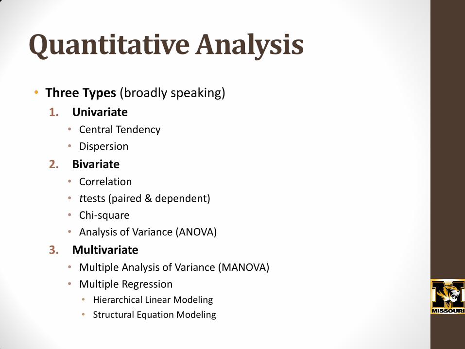
Quantitative Analysis
• Three Types (broadly speaking)
1. Univariate
• Central Tendency
• Dispersion
2. Bivariate
• Correlation
• ttests (paired & dependent)
• Chi-square
• Analysis of Variance (ANOVA)
3. Multivariate
• Multiple Analysis of Variance (MANOVA)
• Multiple Regression
• Hierarchical Linear Modeling
• Structural Equation Modeling
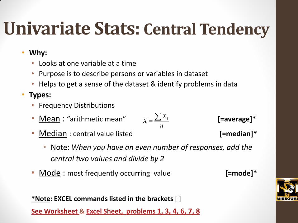
Univariate Stats: Central Tendency
• Why:
• Looks at one variable at a time
• Purpose is to describe persons or variables in dataset
• Helps to get a sense of the dataset & identify problems in data
• Types:
• Frequency Distributions
• Mean : “arithmetic mean” [=average]*
• Median : central value listed [=median]*
• Note: When you have an even number of responses, add the
central two values and divide by 2
• Mode : most frequently occurring value [=mode]*
*Note: EXCEL commands listed in the brackets [ ]
See Worksheet & Excel Sheet, problems 1, 3, 4, 6, 7, 8
n
XX
i
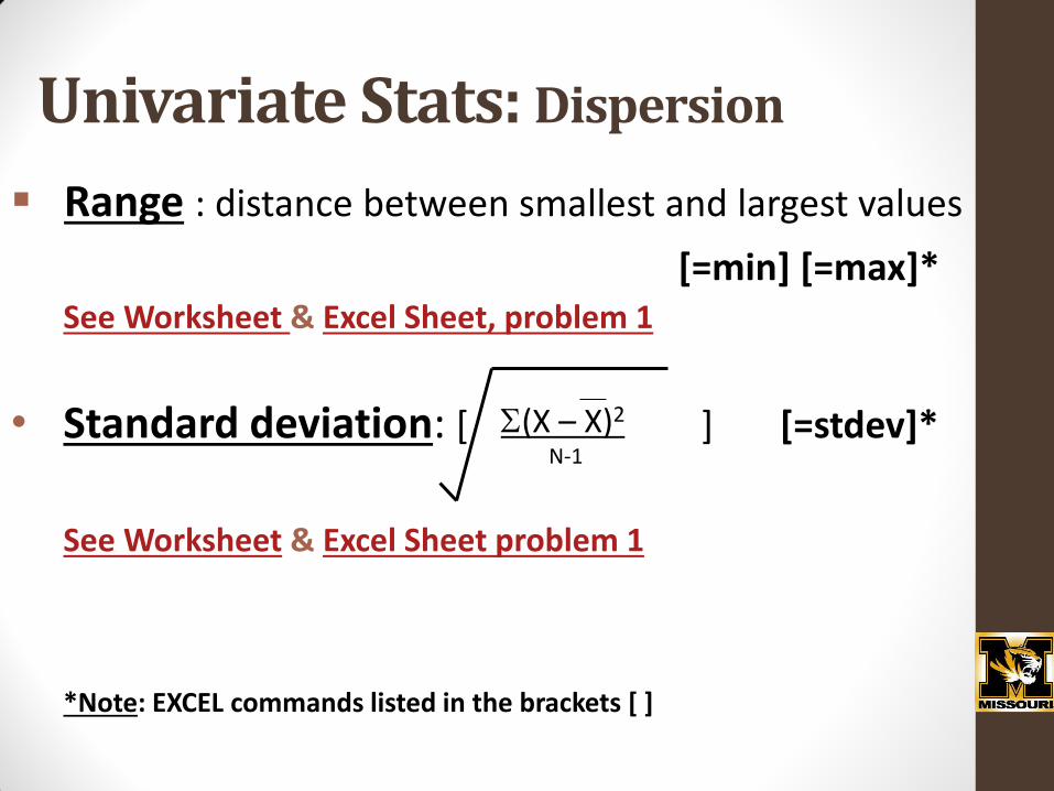
Univariate Stats: Dispersion
Range : distance between smallest and largest values
[=min] [=max]* See Worksheet & Excel Sheet, problem 1
• Standard deviation: [ ] [=stdev]*
See Worksheet & Excel Sheet problem 1
*Note: EXCEL commands listed in the brackets [ ]
(X – X)2
N-1
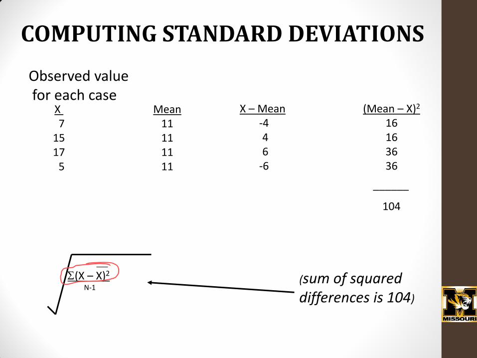
COMPUTING STANDARD DEVIATIONS
Mean 11 11 11 11
X 7 15 17 5
Observed value for each case X – Mean
-4 4 6 -6
(Mean – X)2
16 16 36 36
______
104
Example
(X – X)2
N-1 (sum of squared differences is 104)
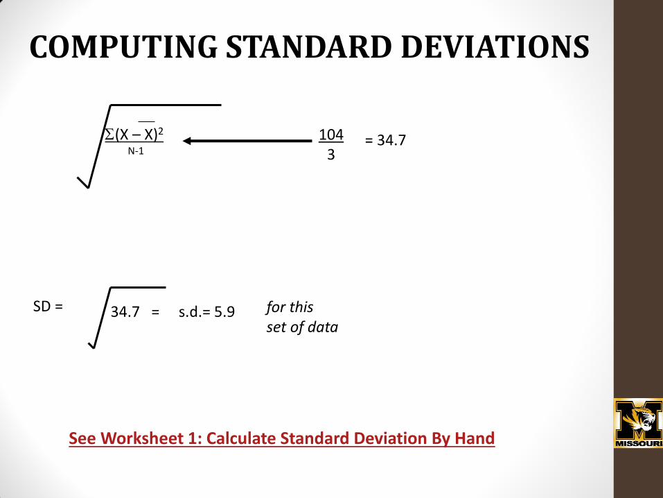
(X – X)2
N-1 104
3 = 34.7
34.7 = s.d.= 5.9 SD = for this set of data
COMPUTING STANDARD DEVIATIONS
See Worksheet 1: Calculate Standard Deviation By Hand
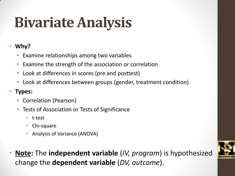
Bivariate Analysis
• Why?
• Examine relationships among two variables
• Examine the strength of the association or correlation
• Look at differences in scores (pre and posttest)
• Look at differences between groups (gender, treatment condition)
• Types:
• Correlation (Pearson)
• Tests of Association or Tests of Significance
• t-test
• Chi-square
• Analysis of Variance (ANOVA)
• Note: The independent variable (IV, program) is hypothesized change the dependent variable (DV, outcome).

• Descriptive information on two variables can be combined in a table • This table gives information on two variables: gender and depression scores
Report
DEPMEAN
3.0541 462 1.19540
3.3068 88 1.13824
3.0945 550 1.18905
SEX gender1 male
2 f emale
Total
Mean N Std. Dev iation
Mean depression subscale scores for males and females (based on 3 bprs depression indicators)
Bivariate Analysis
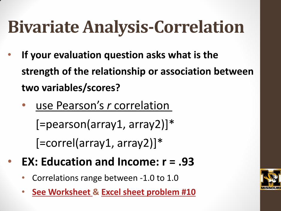
Bivariate Analysis-Correlation
• If your evaluation question asks what is the
strength of the relationship or association between
two variables/scores?
• use Pearson’s r correlation
[=pearson(array1, array2)]*
[=correl(array1, array2)]*
• EX: Education and Income: r = .93 • Correlations range between -1.0 to 1.0
• See Worksheet & Excel sheet problem #10
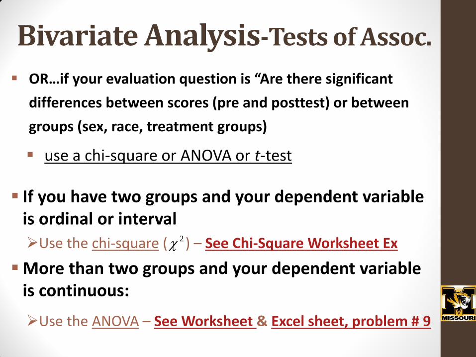
Bivariate Analysis-Tests of Assoc.
OR…if your evaluation question is “Are there significant
differences between scores (pre and posttest) or between
groups (sex, race, treatment groups)
use a chi-square or ANOVA or t-test
If you have two groups and your dependent variable is ordinal or interval
Use the chi-square ( ) – See Chi-Square Worksheet Ex
More than two groups and your dependent variable is continuous:
Use the ANOVA – See Worksheet & Excel sheet, problem # 9
2
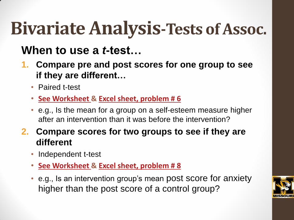
When to use a t-test…
1. Compare pre and post scores for one group to see
if they are different…
• Paired t-test
• See Worksheet & Excel sheet, problem # 6
• e.g., Is the mean for a group on a self-esteem measure higher
after an intervention than it was before the intervention?
2. Compare scores for two groups to see if they are
different
• Independent t-test
• See Worksheet & Excel sheet, problem # 8
• e.g., Is an intervention group’s mean post score for anxiety
higher than the post score of a control group?
Bivariate Analysis-Tests of Assoc.
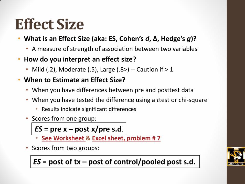
Effect Size • What is an Effect Size (aka: ES, Cohen’s d, Δ, Hedge’s g)?
• A measure of strength of association between two variables
• How do you interpret an effect size?
• Mild (.2), Moderate (.5), Large (.8>) -- Caution if > 1
• When to Estimate an Effect Size?
• When you have differences between pre and posttest data
• When you have tested the difference using a ttest or chi-square
• Results indicate significant differences
• Scores from one group:
• See Worksheet & Excel sheet, problem # 7
• Scores from two groups:
ES = pre x – post x/pre s.d.
ES = post of tx – post of control/pooled post s.d.

REPORTING RESULTS: TELLING THE STORY
Keep it simple
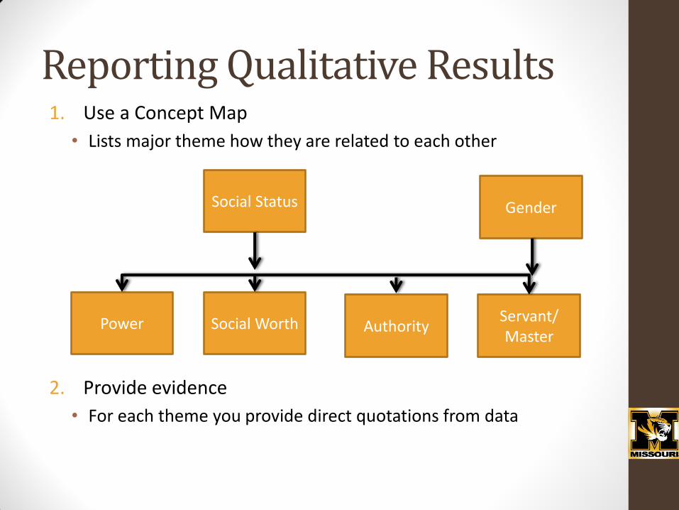
Reporting Qualitative Results 1. Use a Concept Map
• Lists major theme how they are related to each other
2. Provide evidence
• For each theme you provide direct quotations from data
Social Status
Power Social Worth Authority Servant/ Master
Gender
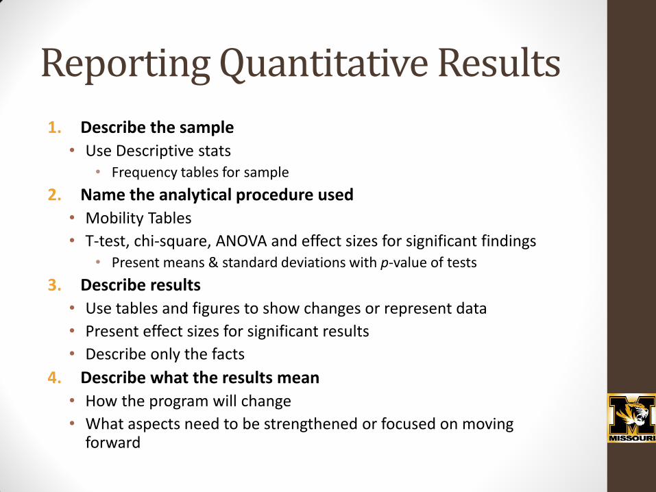
Reporting Quantitative Results
1. Describe the sample
• Use Descriptive stats • Frequency tables for sample
2. Name the analytical procedure used
• Mobility Tables
• T-test, chi-square, ANOVA and effect sizes for significant findings • Present means & standard deviations with p-value of tests
3. Describe results
• Use tables and figures to show changes or represent data
• Present effect sizes for significant results
• Describe only the facts
4. Describe what the results mean
• How the program will change
• What aspects need to be strengthened or focused on moving forward
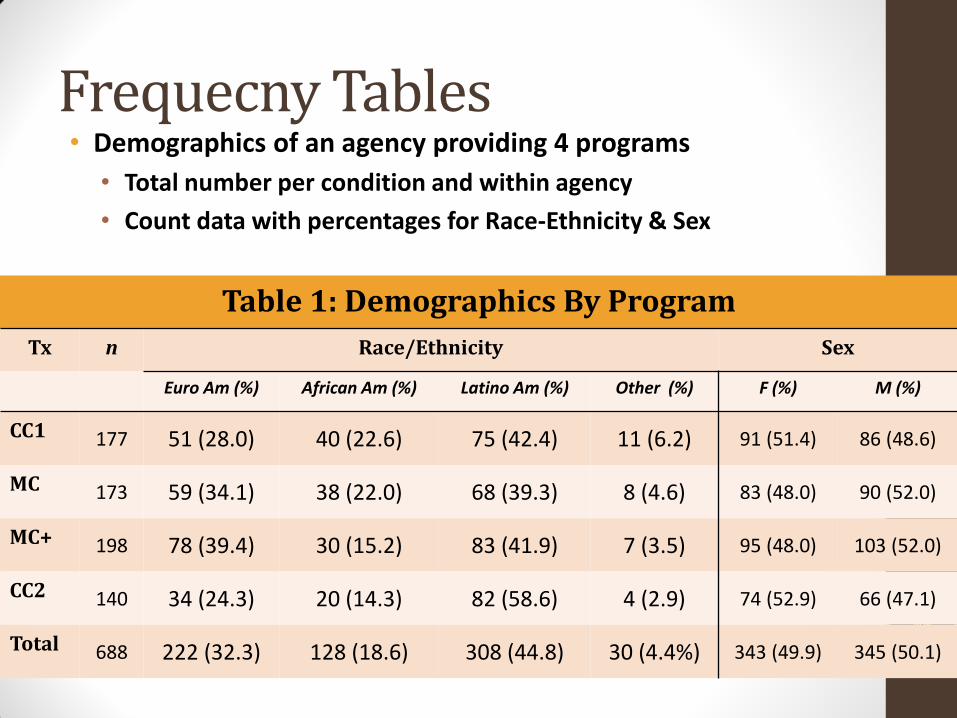
Frequecny Tables • Demographics of an agency providing 4 programs
• Total number per condition and within agency
• Count data with percentages for Race-Ethnicity & Sex
Table 1: Demographics By Program
Tx n Race/Ethnicity Sex
Euro Am (%) African Am (%) Latino Am (%) Other (%) F (%) M (%)
CC1 177 51 (28.0) 40 (22.6) 75 (42.4) 11 (6.2) 91 (51.4) 86 (48.6)
MC 173 59 (34.1) 38 (22.0) 68 (39.3) 8 (4.6) 83 (48.0) 90 (52.0)
MC+ 198 78 (39.4) 30 (15.2) 83 (41.9) 7 (3.5) 95 (48.0) 103 (52.0)
CC2 140 34 (24.3) 20 (14.3) 82 (58.6) 4 (2.9) 74 (52.9) 66 (47.1)
Total 688 222 (32.3) 128 (18.6) 308 (44.8) 30 (4.4%) 343 (49.9) 345 (50.1)
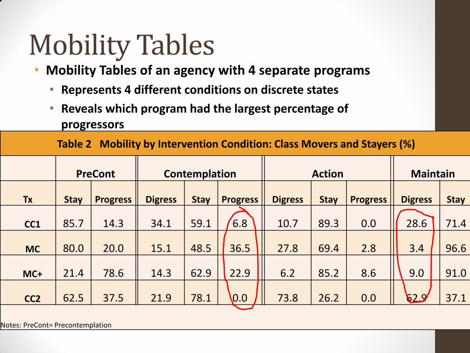
Mobility Tables • Mobility Tables of an agency with 4 separate programs
• Represents 4 different conditions on discrete states
• Reveals which program had the largest percentage of progressors
Table 2 Mobility by Intervention Condition: Class Movers and Stayers (%)
PreCont Contemplation Action Maintain
Tx Stay Progress Digress Stay Progress Digress Stay Progress Digress Stay
CC1 85.7 14.3 34.1 59.1 6.8 10.7 89.3 0.0 28.6 71.4
MC 80.0 20.0 15.1 48.5 36.5 27.8 69.4 2.8 3.4 96.6
MC+ 21.4 78.6 14.3 62.9 22.9 6.2 85.2 8.6 9.0 91.0
CC2 62.5 37.5 21.9 78.1 0.0 73.8 26.2 0.0 62.9 37.1
Notes: PreCont= Precontemplation
Graphics
• Pie Charts
• To show proportions of more than one outcome
• See Worksheet & Excel Sheet, Example #5
• Histograms & Bar Charts
• To show frequencies
• See Worksheet & Excel Sheet Example # 6
• Scatter Plots or line Charts
• To show scores on continuous data
• See Worksheet & Excel Sheet Examples # 1, 2, 3, & 4
And the finish… • Summary Points
1. Be a constructively critical and intelligent consumer
• Know the research and evaluation methods used in your area
• Do not over step what your data tells you
2. Use the Logic Model as Guide
• Rely upon quality indicators and measures and connect them to your logic model (modules I & II)
3. Keep in mind the probabilistic nature of stats
• Good evaluation is more than just statistics • “Blind Reliance upon stats makes the problem worse—it does not need to be
complex….” (Thompson, 2014)
• Present data in simplistic ways • Graphics, charts with trend lines, descriptives, percentages, and ratios
4. Get Help…
• We did not discuss all to be known about analysis or evaluation
• Consultation, Resources & Handouts
• Most important…Positive mindset & sense of humor

The Essence of Authority vs. Evidence-Based Practice

Questions and Comments
• Please Complete the Posttest Form &…
• Feel Contact me for Consultation:
Aaron M. Thompson
School of Social Work
University of Missouri
718 Clark Hall, 65211
PH: 573.882.0124
THANK YOU!!!!


