
Okara, Ikpe Chikwe (2014) Harmonic domain modelling and analysis of the electrical power systems of onshore and offshore oil and gas field /platform. PhD thesis.
http://theses.gla.ac.uk/5593/
Copyright and moral rights for this work are retained by the author
A copy can be downloaded for personal non-commercial research or study, without prior
permission or charge
This work cannot be reproduced or quoted extensively from without first obtaining
permission in writing from the author
The content must not be changed in any way or sold commercially in any format or
medium without the formal permission of the author
When referring to this work, full bibliographic details including the author, title,
awarding institution and date of the thesis must be given
Enlighten:Theses
http://theses.gla.ac.uk/

Harmonic Domain Modelling and Analysis of the Electrical
Power Systems of Onshore and Offshore Oil and
Gas Field /Platform
by
Ikpe Chikwe Okara
A thesis submitted to the
School of Engineering
University of Glasgow
for the degree of
Doctor of Philosophy
October 2014
© Copyright 2014 by Ikpe Chikwe Okara
All Rights Reserved
Electronics and Electrical Engineering
www.glasgow.ac.uk/engineering

ii
Dedications
To Almighy God and the God of Chosen

iii
Abstract
This thesis first focuses on harmonic studies of high voltage cable and power line, more
specifically the harmonic resonance. The cable model is undergrounded system, making it
ideal for the harmonics studies. A flexible approach to the modelling of the frequency
dependent part provides information about possible harmonic excitations and the voltage
waveform during a transient. The power line is modelled by means of lumped-parameters
model and also describes the long line effect. The modelling depth and detail of the cable
model influences the simulation results. It compares two models, first where an approximate
model which make use of complex penetration is used and the second where an Bessel
function model with internal impedance is used. The both models incorporate DC resistance,
skin effect and their harmonic performances are investigated for steady-state operating
condition. The methods illustrate the impotance of including detailed representation of the
skin effect in the power line and cable models, even when ground mode exists. The cable
model exhibit lower harmonics comparable to overhead transmission lines due to strong
influence of the ground mode.
Due to the application of voltage source converter (VSC) technology and pulse width
modulation (PWM) the VSC-HVDC has a number of potential advantages as
compared with CSC-HVDC, such as short circuit current reduction, independent
control of active power and reactive power, etc. With these advantages VSC-HVDC
will likely be widely used in future oil and gas transmission and distribution systems.
Modular multilevel PWM converter applies modular approach and phase-shifted
concepts achieving a number of advantages to be use in HVDC power transmission.
This thesis describes the VSC three-phase full-bridge design of sub-module in
modular multilevel converter (MMC). The main research efforts focus on harmonic
reduction using IGBTs switches, which has ON and OFF capability. The output voltage
waveforms multilevel are obtained using pulse width modulation (PWM) control. The
cascaded H-bridge (CHB) MMC is used to investigate for two-level, five-level, seven-level,
nine-level converter staircase waveforms. The results show that the harmonics are further
reduced as the sub-module converter increases.
The steady-state simulation model of the oil platform for harmonic studies has been
developed using MATLAB. In order to save computational time aggregated models are used.

iv
The load on the platforms consists of passive loads, induction motors, and a constant power
load representing variable speed drives on the platforms. The wind farm consists of a wind
turbine and an induction machine operating at fixed speed using a back-to-back VSC.
Simulations are performed on system harmonics that are thought to be critical for the
operation of the system. The simulation cases represent large and partly exaggerated
disturbances in order to test the limitations of the system. The results show low loss, low
harmonics, and stable voltage and current.
With the developments of multilevel VSC technology in this thesis, multi-terminal direct
current (MTDC) systems integrating modular multilevel converters at all nodes may be more
easily designed. It is shown that self-commutated Voltage Source Converters (VSC) is more
flexible than the more conventional Current Source Converter (CSC) since active and
reactive powers are controlled independently. The space required by the equipment of this
technology is smaller when compared to the space used by the CSCs. In addition, the
installation and maintenance costs are reduced. With these advantages, it will be possible for
several oil and gas production fields connected together by multi-terminal DC grid. With this
development the platforms will not only share energy from the wind farms, but also provide
cheaper harmonic mitigation solutions.
The model of a multi-terminal hypothetical power system consisting of three oil and gas
platforms and two offshore wind farm stations without a common connection to the onshore
power grid is studied. The connection to the onshore grid is realized through a High Voltage
Direct Current (HVDC) transmissions system based on Voltage Source Converter (VSC)
technology.
The proposed models address a wide array of harmonic mitigation solutions, i.e., (i) Local
harmonic mitigation (ii) semi-global harmonic mitigation and (iii) global harmonic
mitigation. In addition, a computationally-efficient technique is proposed and implemented
to impose the operating constraints of the VSC and the host IGBT-PWM switches within the
context of the developed harmonic power flow (HPF). Novel closed forms for updating the
corresponding VSC power and voltage reference set-points are proposed to guarantee that
the power-flow solution fully complies with the VSC constraints. All the proposed platform
models represent (i) the high voltage AC/DC and DC/AC power conversion applications
under balanced harmonic power-flow scenario and (ii) all the operating limits and
constraints of the nodes and its host modular converter (iii) three-phase VSC coupled IGBT-
PWM switches.

v
Acknowledgements
First, I would like to express my deepest gratitude to Professor Olimpo Anaya-Lara
and Calum Cossar, my supervisors, for giving me the opportunity to explore the field of
harmonics in power systems engineering, and for their encouragement and guidance during
the research.
I would like to thank Professor Enrique Acha for his very useful comments and
encouragement at the first, one and half year of the research.
I gratefully acknowledge my colleagues and friends at the Department of Electronics and
Electrical Engineering for making such a productive working environment.
Finally, I would like to thank my wife Joy, my three sons Dominion, Chris and Prosper, my
daughter Joyce and my mother Lucy for their prayers and support.

vi
Contents
Abstract
iii
Acknowledgements ............................................................................................................................... v
List of Figures ...................................................................................................................................... xi
List of Tables ...................................................................................................................................... xvi
Abbreviations and Nomenclature ................................................................................................... xvii
Symbols
xviii
1. Introduction ....................................................................................................................... 1
1.1. Linear and Nonlinear Loads ................................................................................................. 3
1.2. Motivation of the Research Project ...................................................................................... 8
1.3. Objectives of the Research Project ....................................................................................... 9
1.4. Contributions ........................................................................................................................ 9
1.5. Thesis Outline ..................................................................................................................... 10
1.6. Journal Papers .................................................................................................................... 11
1.6.1. Conference Papers .............................................................................................................. 12
1.7. References .......................................................................................................................... 12
2. Contemporary and Future Oil and Gas Field/Platforms Power Systems ................... 14
2.1. Introduction ........................................................................................................................ 14
2.2. Early Oil and Gas Field/Platform Electrical Power Systems ............................................. 18
2.3. The Present Day Oil and Gas Platform Electrical Power Systems ..................................... 19
2.4. Future Development of Electrical Power Systems with zero-load Generator in Oil
and Gas Field/Platform. ...................................................................................................... 22
2.5. Conclusions ........................................................................................................................ 27
2.6. References .......................................................................................................................... 28
3. Power Network Analysis in the Harmonic Domain ....................................................... 37
3.1. Introduction ........................................................................................................................ 37

vii
3.3. Harmonic Modelling and Simulation ................................................................................. 38
3.3.1. Frequency Scan ................................................................................................................... 39
3.3.2. Simple Distortion Calculations ........................................................................................... 40
3.3.3. Harmonic Power Flow Methods ......................................................................................... 43
3.4. Modelling of Harmonic Source .......................................................................................... 44
3.4.1. Power Electronics Converters............................................................................................. 46
3.4.2. VSC-HVDC Stations .......................................................................................................... 46
3.5. Harmonic Producing Loads ................................................................................................ 47
3.6. Methods for Determining Sources of Harmonic Distortion ............................................... 48
3.6.1. Harmonic Power Flow Direction Method .......................................................................... 49
3.6.2. Load Impedance Variation Method .................................................................................... 51
3.7. Total Harmonic Voltage Distortion (VTHD) and Current Distortion(ITHD) .......................... 53
3.8. Total Harmonic Distortion .................................................................................................. 53
3.9. Harmonic Current Magnitude and its Effect on Voltage Distortion ................................... 54
3.10. General Discussion on Fourier Series ................................................................................. 54
3.10.1. Harmonic Power ................................................................................................................. 57
3.11. Conclusions ........................................................................................................................ 57
3.12. References .......................................................................................................................... 58
4. Harmonic Modelling of Power Line and Power Cable Systems ................................... 62
4.1. Introduction ........................................................................................................................ 62
4.2. Harmonic Modelling of Overhead Transmission Lines...................................................... 63
4.2.1. Evaluation of Lumped Parameters ...................................................................................... 64
4.2.2. Matrix of Potential Coefficients (P) ................................................................................... 64
4.2.3. Impedance Matrix of Ground Return (ZG-E) ....................................................................... 65
4.2.4. Skin Effect Impedance Matrix ZSkin .................................................................................... 68
4.2.5. Reduced Equivalent Matrices Zabc and Yabc ........................................................................ 71
4.3. Evaluation of Distributed Parameters ................................................................................. 72

viii
4.3.1. Modal Analysis at Harmonic Frequencies .......................................................................... 72
4.3.2. Non-Homogeneous Lines ................................................................................................... 72
4.4. Test Case 1 .......................................................................................................................... 76
4.4.1. Simulation Results .............................................................................................................. 79
4.5. Harmonic Modelling of Underground and Subsea Cables ................................................. 83
4.5.1. Ground Return Impedance of Underground Cables ........................................................... 85
4.6. Formation of Approximation Cable Model ........................................................................ 88
4.6.1. Voltage Drops in the Cable System .................................................................................... 89
4.6.2. The Impact of Skin Effect in Power Cables System ........................................................... 90
4.6.3. Test Case 2 .......................................................................................................................... 92
4.6.4. Simulation Results .............................................................................................................. 94
4.7. Bessel Function Concept Cable Model ............................................................................... 98
4.7.1. The Impedance (Z) of Three-Layer Conductor ................................................................ 100
4.7.2. The Component Impedance .............................................................................................. 101
4.7.3. The Admittance (Y) of a Cable ........................................................................................ 103
4.7.4. The Potential Coefficient (P) of a Cable ........................................................................... 104
4.8. Test Case 3 ........................................................................................................................ 104
4.8.1. Simulation Results ............................................................................................................ 106
4.9. Conclusions ...................................................................................................................... 110
4.10. References ........................................................................................................................ 111
5. Modular Multi-Level Voltage Source Converters for HVDC Applications ............. 116
5.1. Introduction ...................................................................................................................... 116
5.1.1. Three-Phase Full-Bridge VSC and Operating Principle ................................................... 118
5.2. Design of the DC Capacitor .............................................................................................. 123
5.3. Modular Multi-Level VSC with PWM-Unipolar ............................................................ 124
5.4. Multilevel Output-Voltage Generation ............................................................................. 127
5.5. Modulation Method and Simulations Results ................................................................... 131
5.6. Conclusions ...................................................................................................................... 141
ix
5.7. References ........................................................................................................................ 142
6. Harmonic Analysis of Wind Energy Generator with Voltage Source Converter
Based HVDC Powering Oil and Gas Operations ......................................................... 145
6.1. Introduction ...................................................................................................................... 145
6.2. Offshore Operation of Wind Turbine Feeding Oil Platform ............................................ 149
6.2.1. Wind Turbine Model ........................................................................................................ 149
6.3. Induction Generator Modelling for Offshore Wind Turbine ............................................ 154
6.3.1. SEIG with External Capacitor .......................................................................................... 154
6.3.2. Test Case Impact of Harmonic Injection Stabilizer and Capacitor Excitation ................. 161
6.4. Steady-State Harmonic Model of the VSC-HVDC .......................................................... 165
6.4.1. VSC-HVDC Steady State Model ...................................................................................... 170
6.4.2. Sending and Received Voltage in Terms of Power and Reactive Power ......................... 172
6.5. Harmonic Determination Needed in the Capacitor Bank ................................................ 176
6.6. Harmonic Deriving Point Impedance of Oil Platform ...................................................... 180
6.6.1. Determination of the Base Voltages ................................................................................. 183
6.6.2. Further Simulation Results ............................................................................................... 190
6.6.3. Impact of Advance Static Var Controller (ASVC) ........................................................... 192
6.6.4. Impact of Tuned Reactor Filter ......................................................................................... 198
6.7. Conclusions ...................................................................................................................... 200
6.8. References ........................................................................................................................ 201
7. Harmonic Modelling of Multi-Terminal HVDC-VSC Oil and Gas Platforms ......... 206
7.1. Introduction ...................................................................................................................... 206
7.2. Harmonic Power Flow ...................................................................................................... 209
7.2.1. Switching Function Mode of the Rectifier Process .......................................................... 209
7.3. Potential Application of the Admittance (Y) Matrix of the Five Buses ........................... 211
7.4. Deriving Unknown Nodal Harmonic Voltages and Currents ........................................... 213
7.4.1. Newton-Raphson Conventional Power Flow: Test Case 1 ............................................... 216
7.5. Harmonic Power Flow: Test Case 2 ................................................................................. 220

x
7.6. Conclusions ...................................................................................................................... 231
7.7. References ........................................................................................................................ 232
8. Conclusions and Further Works ................................................................................... 234
8.1. Conclusions ...................................................................................................................... 234
8.2. Recommendations............................................................................................................. 237
8.3. Further Work .................................................................................................................... 238
Appendix 240

xi
List of Figures
Figure 1.1 Voltage signals: (a) Undistorted current signal (b) Distorted current signal ................ 1
Figure 1.2 Relation among voltages in a purely resistive circuit. ..................................................... 4
Figure 1.3. Relation among voltages in a distorted resistive circuit. ................................................ 6
Figure 2.1. Early oil platform electrical power system. ................................................................. 14
Figure 2.2. Present day oil and gas electrical power system layout .............................................. 15
Figure 2.3. Active harmonic filters (AHF) in power systems to monitors the AC line ................ 17
Figure 2. 4a. Block Diagram of multi-terminal HVDC-VSC Scheme for oil and gas .................. 25
Figure. 2.4b. Proposed multi-terminal systems of onshore platform, offshore platform ............ 26
Figure. 3.1 Resonance peaks .............................................................................................................. 40
Figure. 3.3 (a) Typical harmonic spectrum and (b) signal .............................................................. 42
Figure. 3.4 (a) Typical harmonic spectrum and (b) signal .............................................................. 42
Figure 3.5. A single dominant source of harmonics (a) the phase signal (b) magnitude ............. 45
Figure 3.6. Norton equivalent circuits for harmonic current source type load ............................ 47
Figure 3.7. Thevenin equivalent circuit for harmonic voltage source type load ........................... 48
Figure. 3.8. Norton equivalent circuit of a utility customer interface ............................................ 49
Figure. 3.9. Thevenin equivalent circuit of a utility customer interface ........................................ 50
Figure. 3.10 Plot of load parameter variation .................................................................................. 52
Figure. 3.11 (a) Voltage waveform (b) harmonic spectrum ............................................................ 56
Figure 4.1. Line geometry and its image .......................................................................................... 65
Figure 4.2. Line geometry and its image using the complex penetration approach .................... 66
Figure 4.3. ACSR conductors ........................................................................................................... 70
Figure 4.4. Transmission equivalent line π-circuits ........................................................................ 75
Figure 4.5. Power transmission line .................................................................................................. 77
Figure 4.6. Transmission line terminal conditions (a) voltage of source and open-ended .......... 77

xii
Figure 4.7. Three-phase receiving end harmonic voltage excitation, 100km long ....................... 80
Figure 4.8. Three-phase receiving end harmonic voltage excitation, 300km long ....................... 80
Figure 4.9. Three-phase receiving end harmonic voltage excitation, 500km long ....................... 80
Figure 4.10. Three-phase receiving end harmonic voltage excitation, 800km long ..................... 81
Figure 4.11. Three-phase receiving end harmonic current excitation, 100km long .................... 82
Figure 4.12. Three-phase receiving end harmonic current excitation, 300km long .................... 82
Figure 4.13. Three-phase receiving end harmonic current excitation, 500km long .................... 82
Figure 4.14. Three-phase receiving end harmonic current excitation, 500km long .................... 83
Figure 4.15 Internal impedance of the cable system (a) without ground returns ......................... 86
Figure 4.16 Geometric configurations of two SC underground cables and its images ................. 87
Figure 4 .17. An equivalent circuit for impedances of a single-core underground cable ............ 89
Figure 4.18. A cable sheath solidly bonded to the ground .............................................................. 89
Figure 4.19. Geometry of the case study three single-phase cables laying in a flat ..................... 92
Figure 4.20. Harmonic Impedance without voltage and current excitation .................................. 95
Figure 4. 21.1km long cable with first resonant peak appear at h = 350, NH = 500 ..................... 96
Figure 4.22 5km long cable with first resonant peak to appear at h = 70, NH = 400, .................. 97
Figure 4.23 10km long cable with first resonant peak to appear at h = 30, NH = 250 ................. 98
Figure 4.24An equivalent circuit for impedances of single-core cables (SC cable) .................... 100
Figure 4.27. Receiving end in open circuit and 1 p.u. harmonic voltage injection 5km ............. 108
Figure 4.28. Receiving end in open circuit and 1 p.u. harmonic voltage injection 10km ........... 109
Figure 5.1 Two-Level Three-Phase VSC ....................................................................................... 118
Figure 5.2 Reference signals and carrier signal ............................................................................. 119
Figure 5.3. Two-level Phase Switching Function of a VSC one Unipolar PWM Converter
(a)Output voltage of phase a and phase b; (b) The amplitude of all harmonic
spectrum for the output voltage of phase a and phase b; (c) Output voltage of phase
b and phase c; (d) The amplitude of all harmonic spectrum for the output voltage of
phase b and phase c; (e) Output voltage of phase c and phase a; (f) The amplitude of
all harmonic spectrum for the output voltage of phase c and phase a ....................... 122
Figure 5.4: Modular Multi-Level Three-Phase VSC ..................................................................... 127

xiii
Figure 5.5 Five-level Phase Switching Function of a two VSC Unipolar PWM Converters
(a)Output voltage of phase a and phase b; (b) The amplitude of all harmonics for the
output voltage of phase a and phase b; (c) Output voltage of phase b and phase c; (d)
The amplitude of all harmonics for the output voltage of phase b and phase c; (e)
Output voltage of phase c and phase a; (f) The amplitude of all harmonics for the
output voltage of phase c and phase a ........................................................................... 129
Figure 5.6 Five-level line-to-line Switching Function of a two VSC Unipolar PWM
Converters Output voltage of phase a and phase b; (b) The amplitude of all
harmonics for the output voltage of phase a and phase b; (c) Output voltage of phase
b and phase c; (d) The amplitude of all harmonics for the output voltage of phase b
and phase c; (e) Output voltage of phase c and phase a; (f) The amplitude of all
harmonics for the output voltage of phase c................................................................. 130
Figure 5.7 Seven-level Phase Switching Function of a three VSC Unipolar PWM Converters
Output voltage of phase a and phase b; (b) The amplitude of all harmonics for the
output voltage of phase a and phase b; (c) Output voltage of phase b and phase c; (d)
The amplitude of all harmonics for the output voltage of phase b and phase c; (e)
Output voltage of phase c and phase a; (f) The amplitude of all harmonics for the
output voltage of phase c and phase a ........................................................................... 132
Figure 5.8 Seven-level line-to-line Switching Function of a three VSC Unipolar PWM
Converters. Output voltage of phase a and phase b; (b) The amplitude of all
harmonics for the output voltage of phase a and phase b; (c) Output voltage of phase
b and phase c; (d) The amplitude of all harmonics for the output voltage of phase b
and phase c; (e) Output voltage of phase c and phase a; (f) The amplitude of all
harmonics for the output voltage of phase c................................................................. 133
Figure 5.9 Nine-level Phase Switching Function of a fourVSC Unipolar PWM Converters.
Output voltage of phase a and phase b; (b) The amplitude of all harmonics for the
output voltage of phase a and phase b; (c) Output voltage of phase b and phase c; (d)
The amplitude of all harmonics for the output voltage of phase b and phase c; (e)
Output voltage of phase c and phase a; (f) The amplitude of all harmonics for the
output voltage of phase c and phase a ........................................................................... 135
Figure 5.10 Nine-level line-to-line Switching Function of a four VSC Unipolar PWM
Converters. Output voltage of phase a and phase b; (b) The amplitude of all
harmonics for the output voltage of phase a and phase b; (c) Output voltage of phase
b and phase c; (d) The amplitude of all harmonics for the output voltage of phase b
and phase c; (e) Output voltage of phase c and phase a; (f) The amplitude of all
harmonics for the output voltage of phase c................................................................. 136
Figure 5.11. Eleven-level Phase Switching Function of a five VSC Unipolar PWM Converters
Output voltage of phase a and phase b; (b) The amplitude of all harmonics for the
output voltage of phase a and phase b; (c) Output voltage of phase b and phase c; (d)
The amplitude of all harmonics for the output voltage of phase b and phase c; (e)
Output voltage of phase c and phase a; (f) The amplitude of all harmonics for the
output voltage of phase c and phase a ........................................................................... 138

xiv
Figure 5.12. Eleven-level line-to-line Switching Function of a five VSC Unipolar PWM
Converters Output voltage of phase a and phase b; (b) The amplitude of all
harmonics for the output voltage of phase a and phase b; (c) Output voltage of phase
b and phase c; (d) The amplitude of all harmonics for the output voltage of phase b
and phase c; (e) Output voltage of phase c and phase a; (f) The amplitude of all
harmonics for the output voltage of phase c................................................................. 139
Figure 6.1. Schematic of Wind Farm Fed Oil Platform ................................................................ 146
Figure 6.2. Wind generator power curves at various wind speed .............................................. 151
Figure 6.3. Wind turbine rotor mechanical power ....................................................................... 152
Figure 6.4 speed characteristic of wind turbine with low and high gear ratios. ......................... 153
Figure 6.5. Self-excited induction generator with external capacitor. ......................................... 155
Figure 6.6. Equivalent circuit of self-excited induction generator with R-L Load. .................... 156
Table 6.1: Planning Levels for Harmonics Voltage ....................................................................... 158
Figure 6.7. Maximum capacitance at 5th
harmonic ....................................................................... 161
Figure 6.9. Maximum capacitance at 7th
harmonics ...................................................................... 162
Figure 6.10 Exciter load-saturation curve at 7th
harmonic ........................................................... 162
Figure 6.11 Maximum capacitance at 13th
harmonic .................................................................... 163
Figure 6.12 Exciter load-saturation curve at 13th
harmonic ......................................................... 163
Figure 6.14. Exciter load-saturation curve at 29th
harmonic ........................................................ 164
Figure 6.15 Voltage source converter equivalent model ............................................................... 165
Figure 6.16 shows the charging and discharging curves ............................................................... 166
Figure 6.17. Voltage and current of DC capacitor ......................................................................... 166
Figure 6.18. PI controller design and responses ............................................................................ 167
Figure 6.19. Voltage and current in the DC side........................................................................... 169
Figure 6.20. Frequency Contents of Vdc ...................................................................................... 170
Figure 6.21. Frequency Content of Vdc with its complex conjugate ........................................... 170
Figure 6.22. Input current of the (a) rectifier and (b) inverter................................................... 171
Figure 6.23. Output voltage of wind speed side and AC output voltage .................................... 171
Figure 6.24. Active and reactive power of VSC1 and VSC2 with DC link impedance.............. 174
Figure 6.25. Active and reactive power of VSC1 and VSC2 without DC ................................... 174
xv
Figure 6.26. Load angle and voltage magnitude control of the generator-side converter ......... 175
Figure 6.27. Load angle and voltage magnitude control of the platform-side converter ........... 175
Figure 6.28. Series resonance harmonic point with damping in OG 1 ....................................... 177
Figure 6.29. Series resonance harmonic point without damping in OG 1 ................................... 178
Figure 6.30. Series resonance harmonic point with damping in OG 2 ........................................ 179
Figure 6.31. Series resonance harmonic point without damping in OG 2 ................................... 179
Figure 6.32. (a) Harmonic resonance impedance with capacitor bank (b) Harmonic ............ 192
Figure 6.33. Static Var compensator ............................................................................................... 192
Figure 6.34. (a) Harmonic resonance impedance with SVC (b) Harmonic voltage .................... 195
Figure 6.35. (a) Harmonic resonance impedance with SVC and capacitor bank ....................... 196
Figure 6.36. (a) Harmonic resonance impedance with motor starting (b) Harmonic ................ 197
Figure 6.37. (a) Harmonic resonance with tune filter (b) Harmonic voltage spectrum of ......... 199
Figure 6.38. SVC current and capacitor current as afunction of system impedance ................. 200
Figure 7.1. Multi-terminal network with modular multi-level converter used to obtain ........... 208
Figure 7.2. Instantaneous input signal waveforms at (a) bus 1 (b) bus 2 (c) bus 3 (d) bus ........ 218
Figure 7.3. Three Phase Current Waveform .................................................................................. 219
Figure 7.4. Load bus current waveform ......................................................................................... 220
Figure 7.5. Voltage control bus waveform ...................................................................................... 220
Figure 7.6. DC voltage and current at switching frequency ........................................................ 222
Figure 7.7. Frequency Content of Vdc with its complex conjugate ............................................. 222
Figure 7.8. Input Current ................................................................................................................ 223
Figure 7.9. (a)Capacitor voltage (b) Capacitor current ................................................................ 223
Figure 7.10. Voltage conditions at each node of the five VSCs bus .............................................. 224
Figure 7.11. The instantaneous real and reactive powers of the five-bus network .................... 226
Figure 7.13. The instantaneous real and reactive powers of the five-bus network .................... 230

xvi
List of Tables
Table 1.1. Examples of linear loads ..................................................................................................... 5
Table 1.2. Example of nonlinear loads ................................................................................................ 5
Table 6.1: Planning Levels for Harmonics Voltage ....................................................................... 158
Table 6.2. Platform component datas ............................................................................................. 181
Table 6.3. The base impedances and currents................................................................................ 184
Table 6.4. Convert transformer impedances to per unit ............................................................... 184
Table 6.5. Transformer Impedances ............................................................................................... 185
Table 6.7. Convert motor impedances to per unit ......................................................................... 186
Table 6.8. Motor impedances ........................................................................................................... 186
Table 6.9. Harmonic currents for the variable frequency drive................................................... 187
Table 6.10. Convert generator impedance to per unit ................................................................... 187
Table 6.11. Generator impedance ................................................................................................... 188
Table 6.12: Capacitor bank impedances ........................................................................................ 189
Table 7.3: Simulation Parameters ................................................................................................... 221
xvii
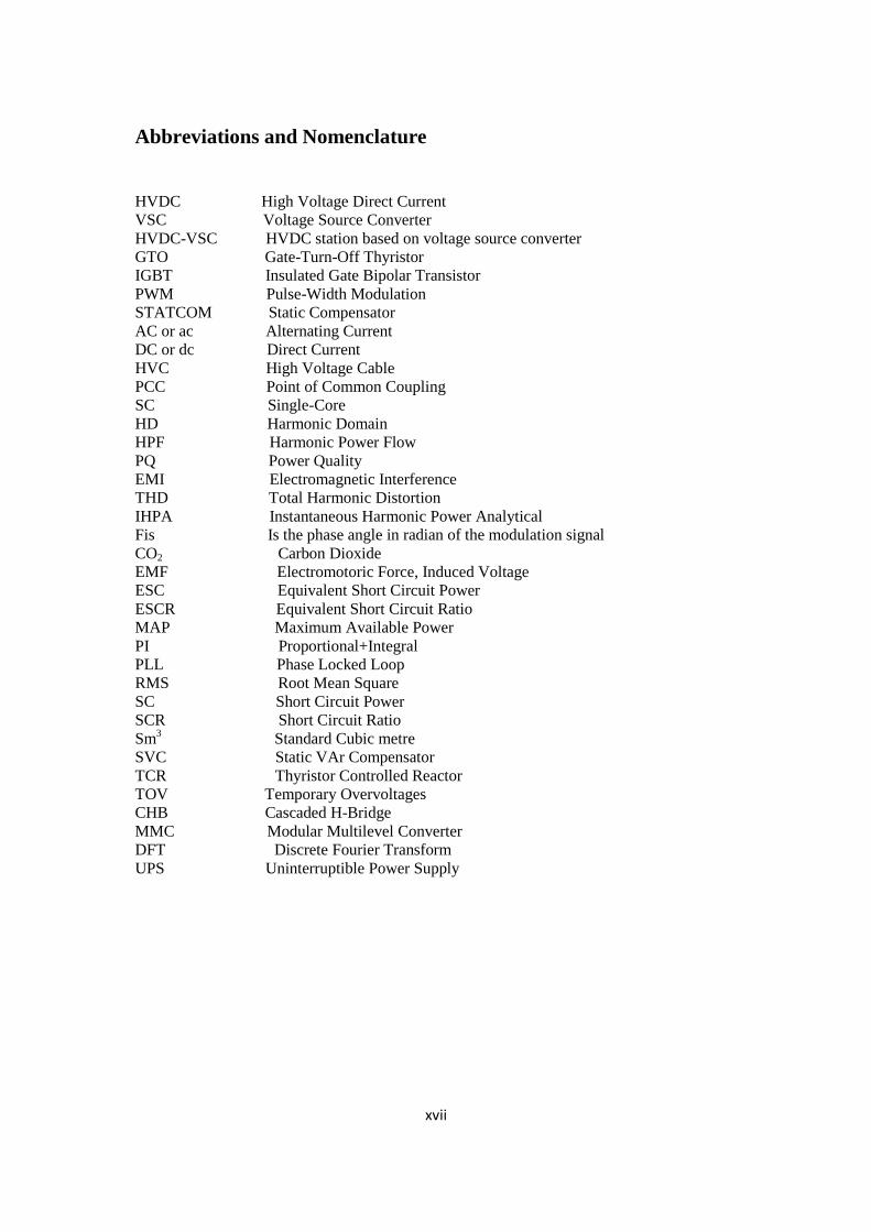
Abbreviations and Nomenclature
HVDC High Voltage Direct Current
VSC Voltage Source Converter
HVDC-VSC HVDC station based on voltage source converter
GTO Gate-Turn-Off Thyristor
IGBT Insulated Gate Bipolar Transistor
PWM Pulse-Width Modulation
STATCOM Static Compensator
AC or ac Alternating Current
DC or dc Direct Current
HVC High Voltage Cable
PCC Point of Common Coupling
SC Single-Core
HD Harmonic Domain
HPF Harmonic Power Flow
PQ Power Quality
EMI Electromagnetic Interference
THD Total Harmonic Distortion
IHPA Instantaneous Harmonic Power Analytical
Fis Is the phase angle in radian of the modulation signal
CO2 Carbon Dioxide
EMF Electromotoric Force, Induced Voltage
ESC Equivalent Short Circuit Power
ESCR Equivalent Short Circuit Ratio
MAP Maximum Available Power
PI Proportional+Integral
PLL Phase Locked Loop
RMS Root Mean Square
SC Short Circuit Power
SCR Short Circuit Ratio
Sm3 Standard Cubic metre
SVC Static VAr Compensator
TCR Thyristor Controlled Reactor
TOV Temporary Overvoltages
CHB Cascaded H-Bridge
MMC Modular Multilevel Converter
DFT Discrete Fourier Transform
UPS Uninterruptible Power Supply
xviii
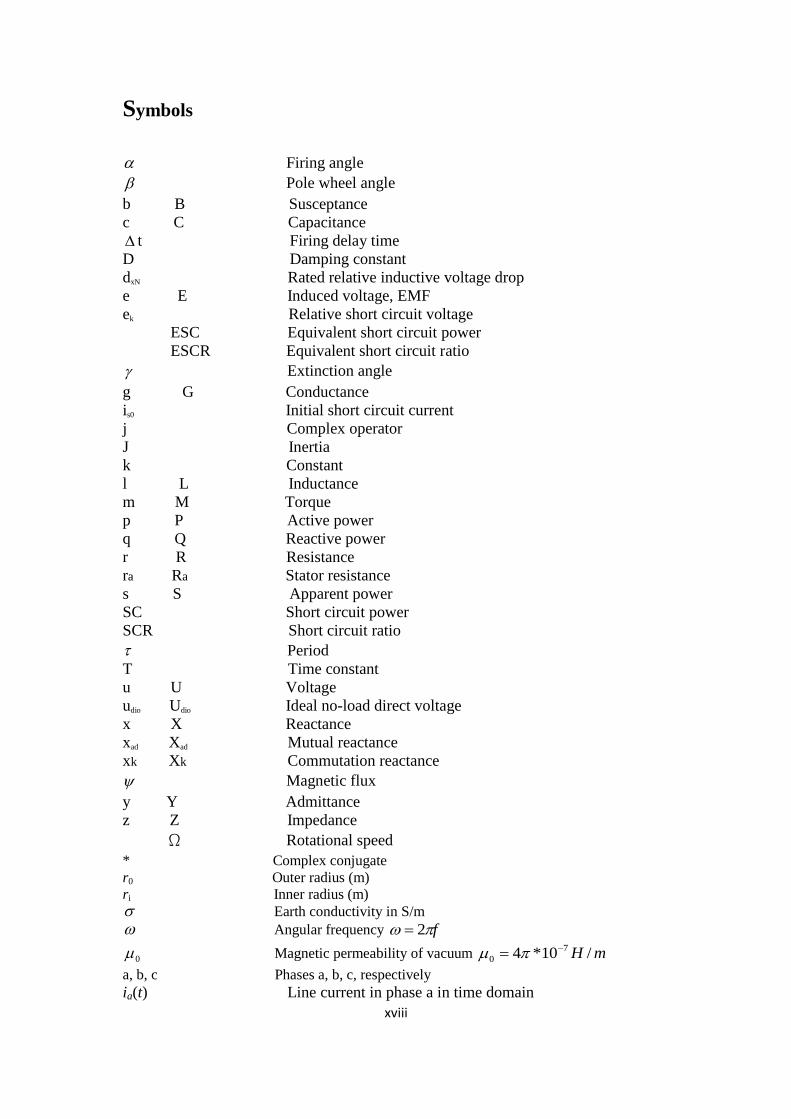
Symbols
Firing angle
Pole wheel angle
b B Susceptance
c C Capacitance
t Firing delay time
D Damping constant
dxN Rated relative inductive voltage drop
e E Induced voltage, EMF
ek Relative short circuit voltage
ESC Equivalent short circuit power
ESCR Equivalent short circuit ratio
Extinction angle
g G Conductance
is0 Initial short circuit current
j Complex operator
J Inertia
k Constant
l L Inductance
m M Torque
p P Active power
q Q Reactive power
r R Resistance
ra Ra Stator resistance
s S Apparent power
SC Short circuit power
SCR Short circuit ratio
Period
T Time constant
u U Voltage
udio Udio Ideal no-load direct voltage
x X Reactance
xad Xad Mutual reactance
xk Xk Commutation reactance
Magnetic flux
y Y Admittance
z Z Impedance
ΩRotational speed
* Complex conjugate
r0 Outer radius (m)
ri Inner radius (m)
Earth conductivity in S/m
Angular frequency f 2
0 Magnetic permeability of vacuum mH /10*4 7
0
a, b, c Phases a, b, c, respectively
ia(t) Line current in phase a in time domain

xix
ib(t) Line current in phase b in time domain
ic(t) Line current in phase c in time domain
va(t) Phase voltage in phase a in time domain
vb(t) Phase voltage in phase b in time domain
vc(t) Phase voltage in phase c in time domain
0 Permittivity of vacuum mF /10*85.8 12
0
r Insulation relative permittivity


1
(b)
Chapter 1
1. Introduction
Voltages and currents in power systems are sinusoidal in nature with a fundamental
frequency typically 50 Hz or 60 Hz [1]. The design of these systems is based on an
assumption that the voltages and currents are not distorted by harmonic components as
shown in Fig. 1.1a. In the majority of existing power systems this assumption is true
and the effects of harmonics can be ignored in the absence of nonlinear loads.
0 0.05 0.1 0.15 0.2 0.25-150
-100
-50
0
50
100
150
Time (sec)
Cur
rent
(A)
ia(t)
ib(t)
ic(t)
Harmonic signal with 3rd, 5th, 7th, 9th, 11th
harmonics
Figure 1.1 Voltage signals: (a) Undistorted current signal (b) Distorted current signal
However, situations do arise when the design must take account of harmonics as shown
in Fig. 1.1b. Such consideration may be necessary at the beginning of a new project or
for a plant that already exists. In the former, the minimisation of the negative effects of
(a)
Time (sec)

2
harmonics is reasonably easy to accomplish. While in the latter it is usually more
difficult due to constraints that may not be removable or reducible.
In AC power system applications where the current naturally goes through zero, the
thyristor remains popular due to its low conduction power losses, its reverse voltage
blocking capability and very low control power requirement. In fact, in very high power
(in excess of 50 MW) AC – DC (phase-controlled converters) or AC – AC (cyclo-
converters) converters, thyristors remain the device of choice. The development of the
gate-turn-off thyristor (GTO) and the insulated-gate bipolar transistor (IGBT) which are
fast, cheaper and more reliable with ON and OFF characteristics has facilitated the
increase of power electronic applications in power systems. With the advent of the high-
power Insulated-Gate Bipolar Transistor (IGBT), a new era in HVDC technology
commenced. This new component was introduced as the main building block of the
valves of a new generation of HVDC converters. The main difference between
thyristors and IGBTs in the operation of the power converter is the turn-off capability of
the latter. This seemingly small difference has completely revolutionised the world of
HVDC: the use of IGBTs instead of thyristors is not a development comparable to the
transition from mercury-arc valves to thyristor valves, but a step change that required a
complete change in the layout and design philosophy of the converter stations, greatly
expanding the range of applications of HVDC [2]. Converters with IGBTs did not
replace converters with thyristors: both systems exist because their field of application
is not the same. To distinguish between both systems, the term Current Source
Converter (CSC) HVDC is used for the thyristor converter HVDC, and Voltage Source
Converter (VSC) for the IGBT converter HVDC. Alternatively, they are referred to as
line-commutated and self-commutated converters respectively. VSC-HVDC is more
flexible than CSC HVDC, requires less space and opens up a wide range of new
applications, such as integration of renewable energy. The increasing use of nonlinear
loads in oil and gas power networks is in turn increasing levels of harmonic distortion.
The most used nonlinear devices are perhaps rectifiers, multipurpose motor speed
drives, and electrical transportation systems (VSC-HVDC). In addition, a scenario that
has increased waveform distortion levels in distribution networks is the application of
capacitor banks for power factor correction used in industrial plants and by power
utilities to enhance voltage profile. When reactive impedance constitutes a tank circuit
with system inductive reactance at a certain frequency, this may result to collision with
one of the characteristic harmonics of the load. In this situation large oscillatory currents
and voltages will be generated which may cause insulation stress.

3
When a voltage and/or current waveform is distorted, it causes abnormal operating
conditions in a power system network such as:
Voltage harmonics can cause additional heating in induction and synchronous
motors and generators.
Voltage harmonics with high peak values can weaken insulation in cables,
windings, and capacitors.
Voltage harmonics can cause malfunction of different electronic components
and circuits that utilize the voltage waveform for synchronization or timing.
Current harmonics in motor windings can create Electromagnetic Interference
(EMI).
Current harmonics flowing through cables and transformer can cause higher
heating over and above the heating that is created from the fundamental
component.
Current harmonics flowing through circuit breakers and switchgear can increase
their heating losses.
Resonant currents which are created by current harmonics and the different
filtering topologies of the power system can cause capacitor failures and/or fuse
failures in the capacitor or other electrical equipment.
False tripping of circuit breakers and protective relays.
1.1. Linear and Nonlinear Loads
A load that draws current from a sinusoidal AC source presenting a waveform like that
of Fig. 1.2 can be conceived as a linear load. Examples of nonlinear loads are shown in
Table 1.1.
0 5 10 15
-10
-5
0
5
10
Time(sec)
Voltage (
volts)
v1(t)
v2(t)
v3(t)
4
0 5 10 15
-1
-0.5
0
0.5
1
1.5
2
Time(sec)
Curr
ent
(A)
I1(t)
I2(t)
I3(t)
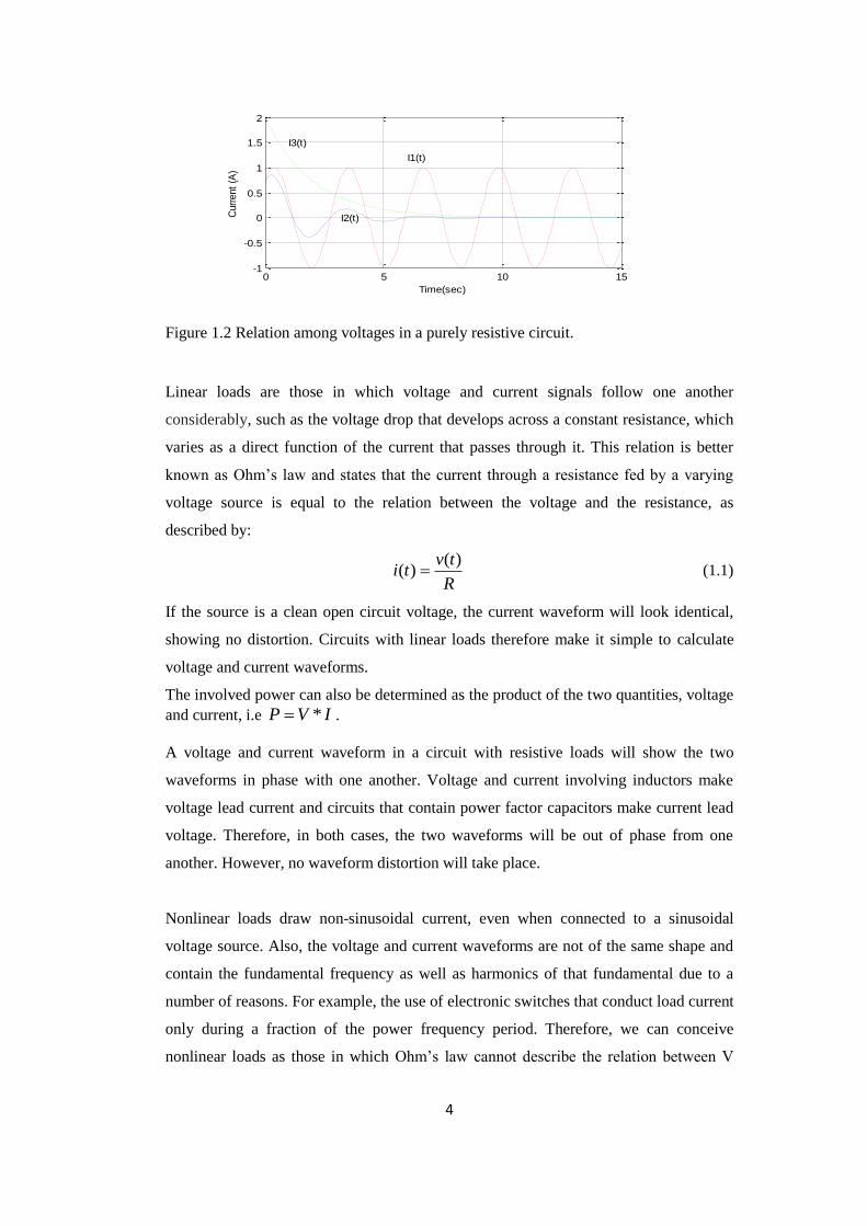
Figure 1.2 Relation among voltages in a purely resistive circuit.
Linear loads are those in which voltage and current signals follow one another
considerably, such as the voltage drop that develops across a constant resistance, which
varies as a direct function of the current that passes through it. This relation is better
known as Ohm’s law and states that the current through a resistance fed by a varying
voltage source is equal to the relation between the voltage and the resistance, as
described by:
R
tvti
)()( (1.1)
If the source is a clean open circuit voltage, the current waveform will look identical,
showing no distortion. Circuits with linear loads therefore make it simple to calculate
voltage and current waveforms.
The involved power can also be determined as the product of the two quantities, voltage
and current, i.e IVP * .
A voltage and current waveform in a circuit with resistive loads will show the two
waveforms in phase with one another. Voltage and current involving inductors make
voltage lead current and circuits that contain power factor capacitors make current lead
voltage. Therefore, in both cases, the two waveforms will be out of phase from one
another. However, no waveform distortion will take place.
Nonlinear loads draw non-sinusoidal current, even when connected to a sinusoidal
voltage source. Also, the voltage and current waveforms are not of the same shape and
contain the fundamental frequency as well as harmonics of that fundamental due to a
number of reasons. For example, the use of electronic switches that conduct load current
only during a fraction of the power frequency period. Therefore, we can conceive
nonlinear loads as those in which Ohm’s law cannot describe the relation between V

5
and I. The breakdown of the current waveform including the six dominant harmonics is
shown in Figure 1.3. Examples of nonlinear loads are shown in Table 1.2.
Table 1.1. Examples of linear loads
Resistive elements Inductive elements Capacitive elements
• Incandescent lighting
• Electric heaters
• Induction motors
• Current limiting reactors
• Induction generators
(wind generators)
• Damping reactors used
to attenuate harmonics
• Tuning reactors in
harmonic filters
• Electrical motors driving
fans
• Water pumps
• Oil pumps
• Power factor correction
capacitor banks
• Underground cables
• Insulated cables
• Capacitors used in
harmonic filters
Table 1.2. Example of nonlinear loads
Power electronics ARC devices
• Power converters/Inverters
• Variable frequency drives
• DC motor controllers
• Cycloconverters
• Power supplies
• UPS
• Battery chargers
• Fluorescent lighting
• ARC furnaces
• Welding machines

6
Variable speed DC motors are mainly used in the oil industry for powering drilling
equipment such as the drill string, draw-works, mud pumps, cement pumps, winches
and the propulsion systems in semi-submersible rigs and barges. They are typically
rated at approximately 800 kW, 750 volts, and several motors may be operated
mechanically in parallel. Each bridge that supplies a motor has a typical current rating
of 2250 amps. The bridges are fed from a three-phase power source which is usually
earthed by a high resistance fault detection device that gives an alarm but does not trip
the source.
0 0.5 1 1.5 2 2.5 3-2
-1
0
1
2
Time (sec)
Magnitude
Figure 1.3. Relation among voltages in a distorted resistive circuit.
Oil and gas platforms harmonic studies are often faced with difficulties linked to
solving high-order equations representing the system as a whole formed by a large
number of facilities and loads. In the past decades it was difficult to model hundreds of
nodes. Today, the development of simulation tools (such as MATLAB/SimPower)
allows large power systems (with hundred nodes) to be modelled.
Oil installations in the North Sea utilize gas-fired turbines in order to generate their
required electric energy. The turbines are placed on the platform and operate with a low
efficiency due to area constraints and operation requirements. The efficiency lies in the
range of 30 % for a typical offshore gas turbine. The turbines are often operated at part-
load, causing further reductions in efficiency [4]. Impinging on this is the need for more
sustainable energy supply (like wind energy) due to fast growing in oil and gas
production. If an onshore/offshore wind farm is to take place, it is important to evaluate
all different ways of harmonics studies and grid connection.
Offshore wind power is in the spotlight as an important renewable energy source. The
location of the wind farms tends to be far from the shore to benefit from the stronger

7
and more constant wind. Also, the power output of the wind farm is increasing with
large scale projects in the range of several hundred MW.
To allow for considerable amounts of offshore wind power and implement a stable
supply to oil and gas installations an offshore grid has to be established. Due to the
distance to shore HVDC transmission may be needed. The establishment of offshore
AC grids offered the opportunity to connect wind farms and oil platforms within the
limited distance of the AC cables. Several of these AC grids can be interconnected and
connected to shore by a multi-terminal DC grid. A HVDC-VSC can be used as a link
between these AC grids and a DC grid.
The use of back-to-back converters for wind turbine variable speed operation is
promising to achieve maximum energy capture in a wide range of wind conditions.
There is however little reference to the harmonics and control of back-to-back
converters for low voltage ride-through capability of wind farms connected to the
network [5][6].
Installation of offshore wind combined with supplying oil and gas installations raises
important issues related to technical solutions, design and operation of the integrated
system. In order to connect oil platforms it is important that the grid can deliver reliable
power quality within given standards [7].
The modern oil and gas production field power systems are supplied with an increasing
number of non-linear loads. These loads are harmonics and interharmonics sources
which require accurate assessment. The harmonic analysis of the systems could be
achieved with the use of Fast Fourier Transform (FFT) due to its faster and
computational efficiency. Moreover, power metering and digital relays in oil and gas
platforms could utilize FFT-Based algorithm to characterize harmonics of the measured
signals [8].
An FFT approach will compute the values at multiple frequencies of the harmonic
spectrum simultaneously, but will consume more resources. To achieve the performance
levels, the amount of memory needed to store the samples used by the FFT algorithm is
significantly high [9].
FFT algorithms are based on the fundamental principle of decomposing the Discrete
Fourier Transform (DFT) computation of a sequence of length N into successively
smaller DFT. Such algorithms vary in efficiency but all of them require fewer
multiplications and additions than direct DFT does. Algorithms in which decomposition
is based on decomposing a sequence x [n] into successively smaller subsequence are

8
called decimation in time algorithm. The basic idea is illustrated by considering special
case of N as 2 to the power of a special integer, i.e. N = 2m. Thus now N is an even
integer. Then F [k] can be computed by separating f [n] into two (N/2) point sequences
that consist of even harmonics of points and odd harmonics of points, in f [n] [10].
With F [k] given by:
NjknN
n
enfN
kF /21
0
1
k = 0,1,2,…, N – 1 (1.1)
Separating f[n] into its even and odd number points, gives:
oddn
NjknNjn
evenn
eenfkF /2/2 (1.2)
1.2. Motivation of the Research Project
Modern oil and gas electrical power systems are being upgraded with a new breed of
power electronics technology based on high switching frequency devices such as GTOs,
IGBTs and PWM control. This new technology is creating new research and exciting
challenges and opportunities at the transmission and distribution levels.
The new HVDC technology is entirely suitable for underground/submarine transmission
and avoids the need for the existence of commutating sources (e.g. synchronous
generators) on the oil platform. However, questions remain concerning the quality of the
voltage waveform supplied by the new breed of HVDC converter technology, due to the
significant amount of high-order harmonic distortion that the PWM control action
introduces. Moreover, oil platforms contain a large number of non-linear loads such as
power electronic rectifiers and saturated induction motors, which may interact adversely
with the distorted incoming supply. The potential benefits promised by the off-site
generation (wind farm) oil platforms are many, such as smaller footprints and increased
security of supply; however, a comprehensive assessment of the oil platform power
system is required at this stage of development. Harmonic generation, harmonic
interactions, harmonic instabilities, harmonic elimination and non-linear load behaviour
are all issues that should be well addressed with the use of harmonic models of relevant
power plant components.

9
1.3. Objectives of the Research Project
This research project is concerned with developing comprehensive models of electrical
power systems of both on-shore and off-shore oil platforms multi-terminal HVDC
transmission links fed via remote wind farm generation. The HVDC converter stations
involve use of IGBT-based VSCs operating at switching frequencies well above power
frequencies but in the low range of kHz.
1.4. Contributions
The main contributions of the research work presented in this thesis are as follows:
A flexible and comprehensive harmonic domain model of single-core, three-
phase high power cables has been developed. The model is very flexible and
takes proper account of the voltage magnitude reduction at harmonic resonance
points due to the skin effect. The model was obtained using the complex depth
concept. The approach may be used to develop accurate models of submarine
cables.
For the cable model, a simple equation which can be used for resonance analysis
is obtained. The model was compared with an alternative formulation
implemented in MATLAB using Bessel function techniques.
A comprehensive harmonic domain model of three-phase VSC-PWM converters
which caters for one, two and three unipolar PWM converters has been
developed. The model takes proper account of the dc capacitor effect and the
voltage ripple on the dc side which comes in the form of a three-phase
equivalent circuit in the harmonic domain, where switching functions are used to
represent the PWM control. The steady-state condition is taken into account by
using an iterative process in order to maintain zero dc current through the
capacitor.

10
Using the VSC model as the basic building block, models for a modular
multilevel converter that uses IGBTs or GTOs were obtained, which resulted in
reduction of more harmonics and increased voltage levels.
The two-terminal HVDC-VSC configurations were; the back-to-back and point-
to-point. An explicit representation of the point-to-point is used since the model
is in the frequency domain.
An oil and gas multi-terminal HVDC-VSC model with integration of wind
turbines was obtained. The mathematical equations are based on harmonic
power flow methods. The power systems and power electronics equipment are
modelled entirely in the harmonic domain. The Newton-Raphson method is used
to solve the non-linear equations resulting from the network constraints.
A flexible harmonic domain analysis solution of typical oil and gas platforms is
obtained. Different cases such as, the effect of Static Var Compensator (SVC)
with harmonic voltages and currents injection, power factor correction (capacitor
bank), active and passive filters with uprising harmonic resonances are
addressed. Each component is modelled based on harmonic domain
considerations.
1.5. Thesis Outline
The thesis is organised as follows:
Chapters 2. This chapter reviews present oil and gas power networks and proposed
future transmission and distribution levels where modular multi-terminal will offer
smart wind turbine integration to oil and gas fields.
Chapter 3 presents the methodologies for harmonic studies.
Chapter 4 presents a new comparative approach to high voltage power cable, power line
and functions in power network. This approach is based on an analysis of Bessel
function simulation in simple steady states, to come up with principles and a
comparative approximate model. It focuses on harmonic resonances. The approximate
model results are compared with those obtained by the Bessel function expressions.
Complete mathematical justifications of the process are provided.
11
Chapter 5 gives an explanation of the technological aspects of steady-state operation of
MMC voltage source converters. The chapter presents a general model of the VSC for
harmonic analysis using the harmonic domain technique. The chapter further proposes a
new Modular Multi-Level VSC with PWM-unipolar for the first time using three-phase
sub-modules, aiming at synthesizing a desired ac voltage from several levels of DC
voltages and harmonic cancellations. The new cascaded-multilevel VSC with minimum
number of isolated DC capacitors is also demonstrated to improve the switching loss
and to increase the range of operation. A novel optimum modulation technique applied
to the multilevel voltage-source converters is suitable for high-voltage power supplies
and flexible AC transmission system devices are also introduced.
Chapter 6 analyses an electrical system for wind turbines with squirrel cage induction
generators interfaced to the grid with back-to-back converters feeding an oil platform.
Matlab simulations evaluate the fault ride-through capability under short circuits in the
power system for different setting conditions of the converters. A model for the HVDC-
VSC point to-point is also presented.
Chapter 7 presents the harmonic domain modelling of an oil/gas multi-terminal network
integrating an offshore wind farm via an HVDC-VSC link. This involves integration of
HVDC-VSC models in the unifying frame of reference afforded by the multi-node,
multi-phase harmonic domain, a frame-of-reference that plays the role of a computing
engine and is amenable to robust iterative solutions using Newton-type methods suitable
for power flow studies.
Chapter 8. In this chapter the conclusions of the work and suggestions for future
research are presented.
1.6. Journal Papers
1. I.C. Okara, and O. Anaya-Lara, Modelling and Analysis of Modular Multilevel
Voltage Source Converter using Harmonic Domain Algebra.
Under review
2. I.C. Okara, and O. Anaya-Lara, Comparative Assessment of Harmonic
Resonance in High Voltage Cable Systems using Bessel and Approximate Models
Submitted to IEEE Transactions on Industry Applications. December 2013.
3. I.C. Okara, O. Anaya-Lara, Harmonic Impedances and Resonances in Oil and
Gas Field Power Systems with Wind Energy Integration.
Submitted to IET Renewable Power Generation. January 2014.

12
4. I.C. Okara, O. Anaya-Lara, Harmonic Modelling of a Multi-terminal Offshore
Network Interconnecting Oil and Gas Platforms and Wind Energy Sources.
Submitted to IET Generation Transmission & Distribution. January 2014.
1.6.1. Conference Papers
2. I.C. Okara, and O. Anaya-Lara, Offshore Wind Farm Integration to Offshore Oil
and Gas Platform using a New VSC-HVDC Model: Harmonic Analysis.
Submitted to International Universities’ Power Engineering Conference.
September 2014.
3. I.C. Okara, and O. Anaya-Lara, Harmonic Injection Stabilizer for Offshore Wind
Farm Induction Generator.
Submitted to Renewable Power Generation Conference. September 2014.
1.7. References
[1] R.P. Bingham,”HARMONICS – Understanding the Facts”
[2] S. Cole and R. Belmans, “Transmission of bulk power: The history and
applications of voltage-source converter high-voltage direct current systems,”
IEEE Ind. Electron. Mag., p. 6, September 2009.
[3] J.Dorn, H. Huang, and D. Retzmann,”Novel voltage source converters for HVDC
and FACTS applications,” Cigr’ eSymposium, Osaka Japan, 2008.
[4] T.F. Nestli, L. Stendius, M.J Johansson, A. Abrahamsson, and P.C Kjaer.
“Powering troll with new technology”. ABB REVIEW, (2):15–19, 2003.
[5] M. Godoy, B. K. Bose, and R. Spiegel, “ Fuzzy logic based intelligent control of a
variable speed cage machine wind generation system”, IEEE Transactions on
Power Electronics, vol. 12, NO. 1, pp. 87-95 (1997).
[6] J. Marvik, T. Bjørgum, B. Næss, T. Undeland, and T. Gjengedal, “Control of a
wind turbine with a doubly fed induction generator after transient failures”, 4th
Nordic Workshop on Power and Industrial Electronics Proc., Norway, (2004)
[7] C. Gopalakrishnan, K. Udayakumar.and T.A. Raghavendiran, “Survey of
harmonic distortion from power quality measurements and the application of
standards including simulation” Transmission and Distribution Conference and
Exhibition 2002: Asia Pacific. IEEE/PES (Volume:2 )
[8] X. Yan, S. Tan, J. Wang, and Y. Wang, “A High Accuracy Harmonic Analysis
Method Based on All-Phase and Interpolated FFT in Power System”. 2011 IEEE.

13
[9] J. Yang, C. Yu, and C. Liu, “A New Method for Power Signal Harmonic Analysis”.
IEEE Transactions on Power Delivery, Vol. 20, No. 2, April 2005.
[10] J. Valenzuela, and J. Pontt, “Real-Time Interharmonics Detection and
Measurement Based on FFT Algorithm”.

14
Chapter 2
2. Contemporary and Future Oil and Gas Field/Platforms
Power Systems
2.1. Introduction
The offshore and onshore oil and gas industry is a mature industry; it has been so for
many decades. During that time hundreds of megawatts of power generation (such as
diesel generators) have been mounted on oil and gas production fields/platforms as
shown in Fig. 2.1.
Figure 2.1. Early oil platform electrical power system.
11kV/600V
11kV/415V 11kV/415V
200kW
300kW
Tx6 Tx5
Tx4 Tx3
Tx2 Tx1
150kW
2MW 2MW Diesel Generator- 2MW
motor
415V
600V
3.3kV
11kV
M
M
M
Transformer
Power Electronics Drive

15
Figure 2.2. Present day oil and gas electrical power system layout
IM2 Z = 26.6% P.F = 0.85 10kV
VFD2
VFD1
TF6
6.6kV/ 3.3kV
ZL3
H
SVC1
SVC2
G
TF5
C3
F
TF3
11kV/ 6.6kV
E
TF4 11kV/ 6.6kV
C2
ZL2
ZL1
C1
D
6.6kV PCC2
11kV
Non-Linear
Load
VSC2 VSC1
60MVA
60MVA
30.5MVA
27MVA
10MVA
IM7 Z = 13.5% P.F = 0.86 5.2kV
IM6 Z – 15.2% P.F = 0.85 6kV
IM5 Z – 18.7% P.F = 0.58 6.5kV
P.F = 0.65 IM4
Z = 20.5% P.F = 0.86 10kV
Z= 30% P.F = 0.60 10kV
GGT
L1
CS1
L1
CS1
Induction
Generator
(Aggregated).
P.F=0.90
TF1
66kV/33kV
500kV
TF2
66kV/33kV
Wind
Farm
50x2 =
100MW
A B
C
PCC1
Emergency
Gas Turbine
Generator
10.8kV
P.F = 0.90
20MW

16
The ever-increasing size of electrical loads on the platforms has called for a gradual
increase in the size of on-site power generators. As the oil and gas production declines,
new frontier areas are being researched, opening opportunities for new research in its
electrical power systems.
Electrical energy generation using gas turbine driven synchronous generators have been
in operation in onshore and offshore fields/platforms for many years as shown in Fig.
2.2. [1-4].
Throughout this time, the rating of generators on the platforms has been on the increase
due to, among other reasons, the widespread use of power electronics-based equipment.
Paradoxically, the development in power electronics in the area of Voltage Source
Converters (VSC) could hold the key to the removal of gas turbine-driven synchronous
generators from the platforms altogether. Current VSC technology has been found to be
highly reliable and commercially attractive and may offer the onshore and offshore oil
and gas industry a viable alternative in electrical energy provision using HVDC
transmission with wind turbine integration which could extend oil and gas exploration
and production well in to the future [5-7].
When designing/modelling any onshore or offshore platform power system, a model is
needed to predict the behaviour of the system with the new loads and to ensure that
equipment ratings are not exceeded. The early platforms actually had few or no facilities
for gas export or reinjection for enhanced oil recovery and for domestic electricity
generation, hence the extra process modules installed when these facilities were needed
have their own dedicated high-voltage switchboards. Moreover, power requirement for
such a heavy consumer as sea water injection is underestimated at the time of
construction [8].
The present oil platform distribution at medium voltage normally consists of
transformer feeders with circuit breaker and other power electronics equipment for main
oil line (MOL) pumps, sea water lift and water injection pumps, and gas export and
reinjection compressors electrical motors with Variable Speed Drives (VSD) [11-15].
Depending on process cooling demand, cooling medium pumps may also be driven by
medium-voltage variable speed drive motors.
Active power filters are now well established in the current oil and gas fields [20-22].
However, some issues still require further research. The filter dynamics depend strongly

17
on the switching frequency; higher frequencies giving better results but at the cost of
higher losses [23]. Specific modulation strategies and control algorithms such as PWM
must be improved. In particular selective harmonic elimination methods can advance
power quality (PQ). More attractively, multilevel converter based topologies allow
Active Harmonic Filters (AHF) to reach higher voltage levels and so permit the
possibility of being applied in the high voltage power systems domain [24]. The AHF
that monitors the AC line current to determine the precise amount of reactive and
harmonic current that the loads need to operate is as shown in Fig. 2.3. The net result is
to off load the source from providing both reactive and harmonic current [25]. The lack
of effective techniques during the early stages of the oil and gas industry slowed its
development for a number of years. The wide spread use of IGBT components and the
availability of new multilevel VSC-PWM are both paving the way to a much brighter
future for the AHF plus PQ in the oil industry. This AHF-VSC introduces current
components, which cancel the harmonic components of the non-linear loads [26].
Within each topology there are issues of required component ratings and the method of
rating the overall filter for the loads to be compensated.
Figure 2.3. Active harmonic filters (AHF) in power systems to monitors the AC line
current
iac
ih
AC Source
Transformer
Medium voltage level
Loads Active Harmonic Filters (AHF)

18
In order to meet the voltage harmonic distortion of 5% for various equipment ratings, it
will be necessary to attenuate as many of the harmonics generated by the power
electronic converters as possible over a wide frequency range. This is because of the
unusually high power source impedance and the high percentage of converter type
loads. The basic objective will be to limit the voltage harmonic distortion to not more
than 5% at the oil and gas platform main generator bus for all platform loads [38].
However, depending on the load variations only one or more generators may be
powering the platform at any one time which tends to increase the distortion levels and
may cause harmonic problems. To reduce the harmonic distortion levels on the system
all equipment characteristics should be carefully modelled, such as the VSC, power line,
power cable, energy generation (e.g. wind turbine) etc. The harmonic analysis of
onshore/offshore harmonic distribution level at the point of common coupling
determines the different levels of harmonic distortion.
2.2. Early Oil and Gas Field/Platform Electrical Power Systems
A large number of diesel generators are used in the oil and gas drilling industry for day-
to-day operations [39-42]. Despite this, the design and the analysis of these electrical
systems are mainly based on short-circuit; load-flow, protective-device coordination,
motor starting and arc flash studies. Although, transient stability studies were
fundamental in determining the nature of the corrective measures aiming to mitigate the
negative effects in the system performance following the occurrence of severe
disturbances, harmonics mitigations were deemed unnecessary [43-45]. Diesel generator
runaway is a serious hazard in oil and gas drilling and production, refining,
petrochemical, and similar industries where flammable hydrocarbon emissions or leaks
may occur [46-47]. Oil and gas production facilities experience frequent sudden
hydrocarbon releases in their operation and this provides external fuel for the diesel
generator to cause runaway [48].
The early Oil and Gas electrical power systems had as their main components, the oil
line pumps powered directly from a diesel generator. By way of example, Fig. 2.1
represents a typical oil platform power system with a total electrical power load of about
6 MW. The platforms do not have variable speed drives and so the AC supply is a
highly dependable and simple source of sinusoidal voltage and current. As shown, there
are three diesel generators connected at the 11 kV bus-bars. Motors are connected at 3.3
kV for sea water lift pumps, DC drilling motors are connected at 600V and motors of up

19
to about 150 kW are connected at 415V. There are no motors connected directly to the
11 kV switchboard [49].
In this platform, electric power is determined by the diesel generator design. Diesel
generators are rated at the brake horsepower developed at the smoke limit. For a given
engine, varying fuel properties within the ASTM D 975 specification range (Standard
Specification for Diesel Fuel Oils) does not alter power significantly [50-54]. However,
fuel viscosity outside of the ASTM D 975 specification range causes poor atomization,
leading to poor combustion, which leads to loss of power and fuel economy.
2.3. The Present Day Oil and Gas Platform Electrical Power Systems
Oil and gas production advancement have led to a continued growth in the size of
compressors, electric motors, drilling machines and pumps used in modern oil and gas
platforms [55]. Power consumption on offshore platforms can vary from 6-7 MW to 20-
40 MW dependent on size and type of the platform with additional emergency
generators and battery power (UPS) for critical situations, when main power fails [56-
57].
The need for power on onshore and offshore installations is almost without exception,
met by local production, mainly in two ways. Heavy machinery such as gas
compressors and pumps are in most cases powered directly from gas turbines or diesel
motors for emergency supply, with if necessary a gear in the middle. The main part of
the electrical energy is consumed by electric motors, electric heating in the production
process and lighting, comfort heating and auxiliary equipment. Also, heating is provided
from heat exchangers, and in the early years some heat was produced in direct-fired
boilers, but this is not common today due to safety reasons.
The need for power varies for different installations, from 10-100 kW for small
wellhead installations to more than 100 MW for the biggest platforms. The total need
for power for large fields is close to 500 MW.
The choice between a compressor and a gas turbine for powering heavy oil and gas
facilities is mainly decided by the short circuit capability of the network. This decides
how large squirrel cage motors can be directly started without unallowable disturbances

20
on the network. The limit for directly started electric motors has gradually increased,
from 5 MW in the early days up to 8 MW today, with increasing electric power rating in
the supply systems. In the case of adjustable speed drives the start-up is far less
disturbing for the network and drives up to 13 MW have been installed recently. For
machines of higher ratings, gas turbines have been the main power source. The limits on
motor size are not absolute; they depend on many other factors as well, company
traditions among others. So the ratio between electric powering and turbine powering
varies widely.
Nowadays, a total platform load that exceeds 100MW is usually powered directly from
a gas turbine-driven synchronous generator with the aid of electric drives of less than 1
MW and gas compressors [58]. The contemporary oil and gas fields/platforms in Fig.
2.2 use two equal-size generators (gas turbine) of half the rated system load and a small
unit diesel generator to supply emergency loads.
Gas turbines consist of a compressor, combustor, and turbine-generator assembly that
converts the rotational energy into electric power output. Gas turbines of all sizes are
now widely used in the power industry. Small industrial gas turbines of 1 – 20 MW are
commonly used in combined heat and power (CHP) applications. They are particularly
useful when higher temperature steam is required (higher than the steam produced by a
reciprocating engine). The maintenance cost is slightly lower than for reciprocating
diesel engines. Gas turbines can be noisy. Emissions are somewhat lower than for
combustion engines, and cost-effective NOX emission-control technology is
commercially available [59].
Micro turbines extend gas turbine technology to smaller scales. The technology was
originally developed for transportation applications, and oil and gas production, but is
now finding a niche in power generation in some part of the world. One of the most
striking technical characteristics of micro turbines is their extremely high rotational
speed, up to 120,000 rpm. They produce high frequency ac power, and a power
electronic inverter converts this high frequency power into a usable form. Individual
micro turbines range from 30 - 200 kW, but can be combined readily into systems of
multiple units. Low combustion temperatures can assure very low NOX emission levels.
They make much less noise than a turbine of comparable size [59]. Most micro turbines
use natural gas. The use of renewable energy sources, such as ethanol, is also possible
[60]. The main disadvantages of micro turbines at the moment are their short track
record and high costs compared with gas combustion engines.
21
A prime mover such as a gas turbine exhibits the effects of wear and tear on the
performance of its engine [61]. In this system, the airflow (and thus the compressor
operating point) is determined by the turbine flow, capacities, while the compressor
absorbed power has to be balanced by the power produced by the gas generator turbine
[62]. The compressor discharge pressure is dictated by the engine firing temperature,
which in turn impacts the engine power. As such any of the components can show wear
and tear over the lifetime of the gas turbine, and thus can adversely affect the operation
of the oil and gas production process [63]. The degradation of engine components has a
consequent effect on engine performance and thereby poor power quality [64].
Understanding the mechanisms that cause degradation, as well as the effects that the
degradation of certain components can cause for the overall system forcing breakdown
are a matter that have opened ways for cleaner power plant research such as wind
turbine [65]. Moreover, transmission lines above 2km the gas turbine losses its
performance [66]. Today’s platforms may use large power electronic variable speed
drives for gas compression duties [67], as illustrated in Fig. 2.2.
The requirement of variable speed drive (VSD), inverter, and rectifier or thyristor
control of some form is used in the platform powered directly from a gas turbine [68].
The combination of these pieces of equipment will cause harmonic currents to be drawn
from the supply [69]. These harmonics will cause two secondary problems. Firstly, the
harmonic currents will flow in cables, transformers and generator windings and in so
doing will immediately produce harmonic volt-drops in these series circuits [70]. This
in turn will cause the voltages at various points in the system to contain harmonic
components, e.g. either side of a transformer, at motor control centres and switchboards,
and other driving motors. Hence the voltages throughout the system will be
contaminated by harmonics. This can be troublesome and difficult to accommodate or
remove. In some situations, the current drawn from the supply by the inverter or
controller can be filtered and smoothed to an almost pure sine wave but this requires
extra equipment which can be large, bulky and expensive [71-72]. The second effect of
the harmonic currents is to induce harmonic emfs by mutual coupling [73-74], and
consequently additional harmonic currents, into cables that are run close to the power
cables feeding the driving motor or its controller.

22
These induced harmonic currents and emfs can be damaging to electronic equipment in
particular and troublesome to computer systems [75]. Often the induced emfs and
currents contain very ‘spikey’ components that have large peak values, and these can be
difficult to remove or suppress.
2.4. Future Development of Electrical Power Systems with zero-load
Generator in Oil and Gas Field/Platform.
The use of conventional HVDC power transmission to supply off-shore oil and gas
platforms has been a matter of research in the past. However, the technology was
deemed to be economically and technically unsuitable on grounds of the relatively short
distances and low voltages and power involved, as well as the need for a commutating
source at the inverter side – this implied the installation of a synchronous
generator/condenser on the platform. Furthermore, the substantial amount of reactive
power provisions and filtering that thyristor-based converters require in order to
function, make up for a rather costly and large foot-print installation.
More specifically, conventional HVDC technology use line-commutated current source
converters (CSC). These converters contain valves; each consisting of a number of
thyristors that are connected in series. The turn-on of the thyristor is controlled by gate
signals while the turn-off takes place at the zero crossing of the AC current which is
determined by the AC network voltage (that is line commutation). Both the sending and
receiving ends of the HVDC system absorb reactive power from the AC system.
Therefore, the HVDC system requires an AC system at least at one end, to have an AC
voltage to commutate. This reactive power demand is a constraint for HVDC stations
connecting to a weak AC system such as oil or a gas offshore AC network [76-77].
HVDC-Capacitor Commutated Converters (CCC) and HVDC-Voltage Sourced
Converters (VSC) technologies can operate at a lower Short Circuit Ratio (SCR) [78-
81]. In addition HVDC-VSC can also actively provide voltage support for the ac
network, within rating and control limits [82-85]. The presence in the ac networks of
many HVDC converters of potentially different technologies or Flexible AC
Transmission components such as STATCOMs and series compensation, in close
electrical proximity, affect the characteristics of the network [82,86]. The new HVDC
transmission technology based on the use of VSC converters seems to be a more adept
technology for feeding onshore and off-shore oil and gas platforms. They do not require

23
large amounts of reactive power compensation with their large footprint, filtering
requirements are much reduced, and there is no need for a commutation source at the
load side [87-88]. Having all these attributes, the HVDC-VSC technology offers a wide
range of applications to the future oil and gas fields/platforms. Further operational
advantages are:
Capability to control reactive power independently of active power
No risk of commutation failures
Faster response due to the use of PWM switching frequency
Capacity to feed a weak AC network or a network without internal generation
It is clear that the HVDC-VSC technology has the potential to improve many of the
problems faced by the oil and gas production field/platform transmission and
distribution systems, but further research and study are required, such as a
comprehensive harmonic domain model and analysis. Other applications of the HVDC-
VSC is the back-to-back tie station, where no DC line or cable is used, this does not
only control power flow, it can also supply reactive power as well as providing
independent dynamic voltage control at its two terminals [89-91].
This new technology which permits the integration of renewable energy sources such as
wind turbines is shown in Fig. 2.4b [92-93]. There are two main control strategies for
this topology, namely
Master-slave: In this strategy one of the VSCs controls the DC bus voltage and
the other VSCs follows predetermined power reference point which can be
constant or assigned by the master converter. If the main converter is found
faulty, next converter automatically takes over the HVDC voltage control.
Coordinated control: Also, in this method the VSCs controls the DC bus voltage
and power transfer in a coordinated way. The HVDC voltage control uses the dc
droop-based method where each converter has a given linear relationship
between HVDC voltage and extracted power.
Gas turbine degradation could be offset and internal combustion engines (ICEs)
removed from the oil and gas drilling fields by the deployment of wind turbines. Wind
energy plays a key role in voltage stability feeding oil and gas drilling platforms.
Today, large wind power plants are competing with fossil-fuelled power plants in
supplying economical clean power in many parts of the world [95].

24
In this sense, wind power is more like central generation than Distributed Generation
(DG). The size of commercial wind turbines has increased significantly from 50 kW in
early 1980s to be up to 4.5 MW recently [96]. This increase obviously creates an
economy of scale for the wind power technology.
Wind turbines offer dynamic control of the active and reactive power and supply
continuity against voltage drop-downs (Fault Ride-Through). These features allow wind
farms to act as standard power plants, providing full support to oil and gas industry and
the grid especially during grid transients. Fig. 2.4a shows the block diagram of an
HVDC-VSC scheme while Fig. 2.4b shows HVDC-VSC links feeding offshore/onshore
platforms/fields from a remote power station via an AC overhead transmission line. The
overall benefit of this scheme is that gas turbines or diesel generators are eliminated
from the offshore platforms as the main energy supply reducing greenhouse emissions
and reducing the overall size of the platform. The VSC converters can operate at
variable frequency to more efficiently drive large compressor or pumping loads using
high voltage motors. Fig. 2.4b shows a clustered oil field that requires supply network
extension from 30kV to 220kV.
The main challenges of wind power technology are intermittency and grid reliability
[97]. Since wind power generation is based on natural forces, it cannot provide power
on demand. On the other hand, utilities must supply power in close balance to demand.
Thus, as the share of wind energy increases, such integration into the oil and gas drilling
electric network will need more attention. Another barrier is transmission availability.
This is because, sometimes, the best locations for wind farms are in remote areas
without close access to a suitable transmission line.
Wind turbine generator systems integration in conventional isolated power systems such
as offshore oil platform can significantly lower operating costs due to increased fuel
savings, but can also have considerable impact on the system stability. In this research,
the stability assessment of an isolated offshore oil platform power system with wind
power main generator is investigated using MATLAB/SIMPOWER. Simulation results
show that the wind power expansion in the isolated offshore oil platform power system
with emergency synchronous generators can keep system voltage and frequency
stability at a desired level. Grid connection between the offshore oil platform power

25
system and wind turbine generators supported by HVDC-VSC will improve the
contribution of wind power to the voltage and frequency stability [98-99].
A novel power transmission scheme for delivering large generated active power of
doubly-fed induction generator (DFIG)-based offshore wind farms (OWFs) fed to oil
and gas offshore/onshore AC grids using a multi-terminal (MT) HVDC-VSC system is
represented in [100-102]. It is found that large scale wind power SEIG generator
integration at the transmission level has the potential to improve the long-term voltage
stability of the grid by injecting reactive power [103].
Figure 2. 4a. Block Diagram of multi-terminal HVDC-VSC Scheme for oil and gas
Wind Farm
100MW
Wind Farm
100MW
Wind Farm
100MW
p. f= 0.65

26
Figure. 2.4b. Proposed multi-terminal systems of onshore platform, offshore platform
and oil and gas production field with modular multi-level converter

27
The harmonic current injection is used to carry out harmonic propagation and control
scheme for the multi-terminal system is proposed and designed to transmit total
generated active power to five grids under various AC operating condition.
2.5. Conclusions
The purpose of this study is to carry out harmonic analysis for power quality and
stability in oil and gas production field. The following are key issues that could
ascertain a safe, stable and continuous power supply:
Main studies including harmonic load flow, harmonic resonance and short circuit study
assist to confirm stability of the power system. Furthermore, it should be noted that any
modifications to each study will influence on the results of other studies.
Accurate cable model is important in many aspects such as harmonic resonance studies,
voltage drop and reactive power losses. Wrong cable model can adversely affect the
system leading to emergency shutdown of the oil and gas production field.
Although in this thesis capacitor bank is recommended for improving power factor for
the purpose of having lower reactive losses, and better control on voltage drops. But
static var compensators (SVC) were utilized to reduce the harmonic resonance
introduced by the capacitor bank in the distribution systems.
By adjusting short circuit impedance of transformer, it is possible to control short circuit
current. But the higher short circuit impedance, the higher losses. That is why utilizing
transformers with higher sizes are recommended such as tap changer transformer. The
tap changer transformer eliminates harmonics distortion as well as assuring required
voltage level on the platform.

28
2.6. References
[1] J M. Wall, R. Lee and S. Frost, “Offshore gas turbines (and major driven
equipment) integrity and inspection guidance notes”, ESR Technology Ltd, First
published 2006.
[2] J.C. Bruno, L. Massegues, and A. Coronas, “Power Quality and Air Emission
tests in a Micro Gas Turbine Congeneration Plant. Proceedings of the
International Conference on Renewable Energy and Power Quality
(ICREPQ’03), 2003.
[3] J.C. Bruno, and A. Coronas, “Distributed Generation of Energy using Micro Gas
Turbines: Ploygeneration Systems and Fuel Flexibility”. Autovia de salou, s/n,
43006 Terragona.
[4] A. D. Oswald and S. D. Hiner, “More efficient applications for naval gas
turbines—addressing the mismatch between available technology and the
requirements of modern naval gas turbine inlets,” in Proceedings of the ASME
Turbo Expo Power for Land, Sea and Air, Barcelona, Spain, 2006, GT2006-
90305.
[5] G. Ding, G. Tang, Z. He, and M. Ding, “New technologies of voltage source
converter (VSC) for HVDC transmission system based on VSC “Power and
Energy Society General Meeting Conversion and Delivery of Electrical Energy in
the 21st Century, 2008 IEEE
[6] S. G. Johansson, G. Asplund, E. Jansson, and R. Rudervall, “Power system
stability benefits with VSC DC-transmission systems,” in CIGR´E 2004, Paris,
France, August 2004.
[7] G. Asplund, K. Eriksson, H. Jiang, J. Lindberg, R. P°alsson, and K. Svensson,
“DC transmission based on voltage source converters,” in International
Conference on Large High Voltage Electric Systems. CIGR´E 98, vol. 4, Paris,
France, 1998.
[8] P. Jakobsen, G, Peck, and E, Snow, “Electrical Power System Challenges During
the Expansion of Offshore Oil & Gas Facilities” Petroleum and Chemical
Industry Conference Europe Conference IEEE Proceedings (PCIC EUROPE),
2012.
[9] R.E.Cossé, Terence G. Hazel and Gorges Thomasset,"IEC Medium-Voltage
Circuit-Breaker Interrupting Ratings – Unstated Short-Circuit Considerations"
IEEE Transactions on Industry Applications, Vol.36 No.3 May/June 2000
[10] DS/EN62271-100 (2009) High-voltage switchgear –= Part 100: Alternating-
current circuit-breakers.

29
[11] M. Hernes and B.Gustavsen, “Simulation of shaft vibrations due to interaction
between turbine-generator train and power electronic converters at the Visund oil
platform”, IEEE Proceedings of the Power Conversion Conference, 2002. PCC-
Osaka 2002
[12] K.W.L. Burbridge, “Users View of Variable Speed Drives on Petrochemical
Plant” Electrical Machines and Drives, 1993. Sixth International Conference No.
376.
[13] M.Tsukakoshi, M.Al Mamum, K. Hashhimura, H. Hosoda, and T. Kojima,
“Performance evaluation of a large capacity VSD system for Oil and Gas
industry” Energy Conversion Congress and Exposition, 2009. ECCE 2009. IEEE.
[14] J.O. Lamell, T.Trumbo, and T.F. Nesti, “Offshore Platform Powered with New
Electrical Motor Drive System” Petroleum and Chemical Industry Conference,
2005. Industry Applications Society 52nd Annual. IEEE
[15] M. Didden, H. De, C. Jean, and D.J. Emmanuael, “Installing variable speed
drives: Energy efficiency profits versus power quality losses”, Electricity
Distribution, 2005. CIRED 2005. 18th International Conference. IEEE
[16] H.L. Jou, J.C.Wu, J.J. Yang, and W.P.Hsu, “Novel Circuit Configuration for
Hybrid Reactive Power Compensator”, Power Electronics and Motion Control,
2006. IPEMC 2006. CES/IEEE.
[17] X. Liu, L. Sun, Y. Sun, and Z. Dean, “The synthetical compensation research on
high-order harmonic and reactive power”, Industrial Technology, 2008. ICIT
2008. IEEE.
[18] S. Shankar, A. Kumar, and W. Gao, “Operation of unified power quality
conditioner under different situations”, Power and Energy Society General
Meeting, 2011 IEEE.
[19] M. Izhar, C.M. Hadzer, M. Syafrudin, S. Taib, and S. Idris, “Performance for
Passive and Active Power Filter in Reducing Harmonics in the Distribution
System”, Power and Energy Conference, 2004. PECon 2004. IEEE Proceedings
[20] I. Faegheh, and S.H. Hosseinian, “Using the Instantaneous Power Theory in order
to control the current in the parallel active filter to compensate reactive power and
reduction of harmonics”, Power Electronics, Drives and Energy Systems
(PEDES), 2012 IEEE.
[21] D. Gao, Q. Lu, and X. Sun, “Design and performance of an active power filter for
unbalanced loads”, Power System Technology, 2002. IEEE Proceedings.
PowerCon 2002.
[22] J.C. Wu, H.L.. Jou, Y.T. Feng, W.P. Hsu, M.S. Huang, and W.J. Hou, “Novel
Circuit Topology for Three-Phase Active Power Filter”. IEEE Transactions on
Power Delivery, Jan. 2007.

30
[23] C.Po-Tai, S. Bhattacharya, and D. Divan, “Experimental Verification of
Dominant Harmonic Active Filter (DHAF) for High Power Applications”,
Industry Applications Conference, 1998. Thirty-Third IAS Annual Meeting. The
1998 IEEE
[24] Z.H. Yuan, “A Shunt Active Harmonic Filter Based on a Voltage Detection
Method for Harmonic Voltage Control”, Electric Utility Deregulation,
Restructuring and Power Technologies, 2004. (DRPT 2004). Proceedings of the
2004 IEEE
[25] J.H. Xu, S. Saadate, and B. Davat, “Compensation of AC-DC converter input
current harmonics using a voltage-source active power filter”, Power Electronics
and Applications, 1993. Fifth European Conference
[26] M.E. Ortuzar, R.E. Carmi, L.W. Dixon, and L.Moran, “Voltage-Source Active
Power Filter Based on Multilevel Converter and Ultracapacitor DC Link”, IEEE
Tranasactions on Industrial Electronics.
[27] R.Majumder,“Reactive Power Compensation in Single-Phase Operation of
Microgrid”, IEEE Tranasactions on Industrial Electronics.
[28] A.Cetin, M. Ermis. “VSC Based D-STATCOM with Selective Harmonic
Elimination”, Industry Applications Conference, 2007. 42nd IAS Annual
Meeting. Conference Record of the 2007 IEEE
[29] R.E. Betz, T.J. Summers, and G. Mirzaeva, “Active filtering and VAR control of
a cascaded H-bridge multi-level StatCom”, Power Electronics and Drive Systems,
2009. PEDS 2009.
[30] S.H. Hosseini, and M. Sabahi, “Three-Phase Active Filter using a Single-Phase
STATCOM Structure with Asymmetrical Dead-band Control”, Power Electronics
and Motion Control Conference, 2006. IPEMC 2006. CES/IEEE 5th
International.
[31] T. Jin, L. Li, and K. Smedley, “A universal vector controller for three-phase PFC,
APF, STATCOM, and grid-connected inverter”, Applied Power Electronics
Conference and Exposition, 2004. APEC '04. Nineteenth Annual IEEE.
[32] P.S. Sensarma, K.R. Padiyar, and V. Pamanarayanan “A STATCOM for
composite power line conditioning”, Industrial Technology 2000. Proceedings of
IEEE International.
[33] X. Wang, and S. Hua“Extended state feedback control for active power filter”,
Computer Science and Automation Engineering (CSAE), 2011 IEEE
International.
[34] O. De, E.M. Sebastiao, and J.O.R. Guimuraes, “Effects of Voltage Supply
Unbalance on AC Harmonic Current Components Produced by AC/DC
Converters”, IEEE Tranasactions on Power Delivery. 2007.

31
[35] K. M. Nor, L.W. Jeun, M. Abdel-Akher, and A.H. Abudul-Rashid, “Reusing
Three-Phase Power-Flow Object Components for Unbalanced Harmonic
Analysis”, Power and Energy Conference, 2006. PECon '06. IEEE International.
[36] T. Zheng, E.B. Makram, and A.A. Girgis, “Evaluating power system unbalance in
the presence of harmonic distortion”, IEEE Tranasactions on Power Delivery.
April 2003
[37] K.Nohara, A. Ueda, A. Torii, and K. Doki, “Compensating Characteristics of a
Series-Shunt Active Power Filter Considering Unbalanced Source Voltage and
Unbalanced Load”, IEEE Power Conversion Conference - Nagoya, 2007. PCC
'07.
[38] IEEE, Recommended Practices and Requirements for Harmonic Control in
Electrical Power Systems, IEEE Std. 519-1992.
[39] M.L. Rizzone, “Electric Drilling Rig Developments”, IEEE Transactions On
Industry and General Applications Vol. IGA-3, No. 2
[40] Y. Xiong, H.Wang ,and S. Lu, “Study on Micro-Biological Degradation of Diesel
Oil cooperated with Plants”
[41] P.M. David, “Increasing the Electrical Output of a Cogeneration Plant”, IEEE
Trans. On Industry Applications, vol. 38, no. 3, pp. 726- 735, May/Jun 2002.
[42] S.R. Stanley, “Electrical Transient Stability and under frequency Load Shedding
Analysis for a Large Pump Station”, IEEE Trans. On Industry Applications, vol.
33, no. 1, pp. 194-201, Jan/Feb 1997.
[43] S.P.Thomas,“Power System Studies for Cement plants”, IEEE Industry
Applications magazine, pp. 56-65, July/August 2007
[44] D.P. Mathew. and J.L. Kohler , “An Improved Model for Analyzing Industrial
Power Systems”, IEEE Trans. On Industry Applications, Vol. 31, No. 5, pp.
1140-1146, September/October 1995
[45] J. R. Dunki-Jacobs and C. E.Davis, “An Argument and Procedure for Conceptual
Power System Design Studies”, IEEE Trans. On Industry Applications, Vol. 30,
No. 2, pp. 253-261, March/April, 1994
[46] D.L.Hodgson, M. McKinney, S. DeGrate, “Increasing electrical safety by
reducing the risk of arc flash hazards”, Petroleum and Chemical Industry
Conference (PCIC), 2011. IEEE
[47] G.S. Lawler, “Fires of Electrical Origin in Factories”, Electrical Engineering.
IEEE.
[48] D. Buscher, “Avoiding loss of voltage sensing runaway for generator excitation
systems”, Industry Technical Conference (PPIC), 2011 Annual IEEE.

32
[49] G. Gerrard, “Offshore Electrical Engineering” British Library 1992.
[50] A. Marcus “Diesel Fuel Basics”, PASSAGEMAKER • Fall 1999 PassageMaker
Magazine, Inc.
[51] P. Lu, J.Wu, and W. Pan, “Particulate Matter Emissions from a Coal-Fired Power
Plant”, Bioinformatics and Biomedical Engineering (iCBBE), 2010. IEEE..
[52] J.Deng, A. Ordys, and Y. Wang, “Input choices of Particulate Matter Models for
Diesel Engines”, Control and Decision Conference (CCDC), 2012. IEEE
[53] S. Sakulniyomporn, K. Kubaha, and C. Chullabodhi, “Estimating the health
damage costs of electricity generation in Thailand”, Energy and Sustainable
Development: Issues and Strategies (ESD), IEEE 2010 Proceedings.
[54] V. Dawar, B. Lesieutre, T. Holloway, and E. Bickford, “An efficient approach to
reduce emissions by coupling atmospheric and electricity market models”, North
American Power Symposium (NAPS), 2012. IEEE.
[55] J.O.Lamell, T.Trumbo, T.F. Nestli, “Offshore platform powered with new
electrical motor drive system”, Petroleum and Chemical Industry Conference,
2005. Industry Applications.IEEE
[56] S.K.Salman, F.Jiang, W.J.S. Rogers, “Investigation of the operating strategies of
remotely connected embedded generators to help regulating local network
voltage”, Opportunities and Advances in International Electric Power Generation,
International Conference on IEEE March 1996.
[57] W.J.S.Rogers,“Impact of embedded generation on design, operation and
protection of distribution networks”, Embedded Generation on Distribution
Networks (Digest No. 1996/194), IEE Colloquium on the Impact of IEEE Oct;
1996.
[58] D.M.Soto,A.Hasanzadeh, and C.S. Edrington,“Gas turbine-synchronous generator
system emulation using power electronics converters”, North American Power
Symposium (NAPS), Sept; 2012.IEEE.
[59] IEA, Distributed Generation in Liberalised Electricity Markets, International
Energy Agency, France, 2002.
[60] M.W.Davis, “Micro turbines – an economics and reliability evaluation for
commercial, residential and remote load applications”, IEEE Transaction on
Power Systems, vol. 14, no. 4, pp. 1556-1562, 1999.
[61] H.D. Hollis, R.G. Arno, S.J. Briggs, and P.S. Hale, “Operational maintenance data
for power generation distribution and HVAC components”, Industrial and
Commercial Power Systems Technical Conference, May 1996, IEEE
[62] H.J. Nern, H. Kreshman, F.Fischer, H.A. Eldin, “Modelling of the long term
dynamic performance of a gas turbo generator set”, Control Applications, 1994.,
Proceedings of the Third IEEE, Aug; 1994.
33
[63] J. Sumner, A. Encinas-Oropesa, M. Seraffon, N.J. Simms, J.R. Nicholls,
“Lifetime prediction for gas turbine materials in power generation”, Sustainable
Power Generation and Supply (SUPERGEN 2012),
[64] N. Gebraeel, A. Elwany, J. Pan, “Residual Life Predictions in the Absence of
Prior Degradation Knowledge” IEEE Transactions on Reliability. March 2009.
[65] E. Muljadi, C.P. Butterfield, J. Chacon, and H. Romanowitz, “Power quality
aspects in a wind power plant”, Power Engineering Society General Meeting,
2006. IEEE.
[66] S. Mohammad, S. Zadeh,“Economic Operation of Long Distances Power
Networks Using On-line Control of Superconducting Magnetic Energy Storage”,
EUROCON 2007. IEEE.
[67] M. Bressani, A. Odorico, and M. Sica, “High-speed, large-power induction
motors for direct coupling to variable-speed gas compressors”, Power Electronics
and Applications, 1993. IEEE.
[68] J. Arai, K. Iba, T. Funabashi, Y. Nakanishi, K. Koyanagi, and R. Yokoyama,
“Power electronics and its applications to renewable energy in Japan”, IEEE
Circuit and Systems Magazine.
[69] D.D.Shipp, W. Vilcheck, M.E. Swartz, and N.H. Woodley, “Expert system for
analysis of electric power system harmonics”, IEEE Industry Applications
Magazine, March/April 1995.
[70] H. Funato, C. Sasaki, Y. Chiku, and S. Ogasawara, “Analysis of loss of receiving
transformer caused by harmonic current and voltage for loss reduction”, Power
Electronics and Motion Control (EPE/PEMC), IEEE, Sept; 2010.
[71] J.C.Das,”Passive Filters-Potentialities and Limitations”,IEEE Trans. Ind.
Applications, vol. 40, No. 1, Jan/Feb; 2004.
[72] D. A. Gonzalez and J. C. McCall, “Design of filters to reduce harmonic distortion
in industrial power systems,” IEEE Trans. Ind. Applicat., vol. IA-23, pp. 504–
512, May/June 1987.
[73] E.Semail, X. Kestelyn, and A. Bouscayrol, “Right harmonic spectrum for the
back-electromotive force of an n-phase synchronous motor”, Industry
Applications Conference, 2004. 39th IAS
[74] P. Ioannides, and C.A. Balanis, “Mutual coupling in adaptive circular arrays”,
Antennas and Propagation Society International Symposium, 2004. IEEE
[75] L. Wa, S. Saodah, and J. Nurahmat, “Current harmonic analysis of electronics
loads on induction generator”, Condition Monitoring and Diagnosis (CMD), Sept;
2012. IEEE.

34
[76] A. Reidy and R. Watson, “Comparison of VSC base HVDC and HVAC
interconnections to a large offshore wind farm”, Proc. IEEE Power Eng. Soc.
General Meeting, Jun.2005, pp. 71-78.
[77] F. Schettler, H. Huang, and N. Christl, “HVDC Transmission Systems using
Voltage Sourced Converters –Design and Applications”. In Proc. IEEE PES
Summer Meeting, vol. 2, Seattle, WA, 2000, pp. 715-720.
[78] Y.Jiang-Häfner, M. Hyttinen, and B. Pääjärvi, “On the Short Circuit Current
Contribution of HVDC Light”,
[79] CIGRE “Guide for planning dc links terminating at AC systems locations having
low short-circuit capacities—part I: AC/DC interaction phenomena”. Report 68,
June 1992
[80] P. F. de Toledo, B. Bergdahl, and G. Asplund “Multiple Infeed Short Circuit
Ratio – Aspects Related to Multiple HVDC into one AC Network”, ABB Power
System, HVDC Division
[81] “Guide for planning DC Links terminating at AC system having low short-circuit
capacity, Part I: AC/DC interaction phenomena”, CIGRE Guide No 68, Paris
1992
[82] J. Pan, R. Nuqui, K. Srivastava, T. Jonsson, P. Holmberg, and Y. Hafner, “AC
Grid with Embedded VSC-HVDC for Secure and Efficient Power Delivery”,
EEE Energy 2030, 17-18 November, 2008 Atlanta, USA.
[83] Stefan G Johansson, Gunnar Asplund, Erik Jansson, Roberto Rudervall, “Power
System Stability Benefits with VSC DC Transmission Systems”, CIGRE
Conference, 2004, Paris, France.
[84] Peter Sandeberg and Lars Stendius, “Large scale Offshore Wind Power Energy
evacuation by HVDC Light®”, European Wind Energy Conference & Exhibition,
March-April 2008, Brussels Belgium.
[85] Gunnar Asplund, “Electric Transmission System in Change”, Key Notes, IEEE
Power Electronics Specialists Conference, June 2008, Rhodes, Greece
[86] M. P. Bahrman, J. G. Johansson, and B. A. Nilsson “Voltage Source Converter
Transmission Technologies - the right fit for the Application”, ABB.
[87] R. S. Rani, and B. Jyothi, “VSC Based DSTATCOM & Pulse-width modulation
for Power Quality Improvement”, International Journal of Engineering Trends
and Technology- Volume2Issue2- 2011
[88] J. Dixon , L. Morán, J. Rodríguez, and R. Domke “Reactive Power
Compensation Technologies, State of-the-Art Review”.
[89] J. Liu, L. Yao, T. Wu, Y. Guo,Y. An, and C. He “Application of back-to-back
VSC-HVDC in Power Grids Synchronization Parallel Operation”, IEEE 2010
International Conference on Electrical and Control Engineering

35
[90] M. Bahrman , A. Edris , and R. Haley, “Asynchronous Back-to-Back HVDC
Link With Voltage Source Converters”, PRESENTED AT MINNESOTA POWER
SYSTEMS CONFERENCE, NOV 1999, USA.
[91] A. L'Abbate and G. Fulli “Modeling and Application of VSC-HVDC in the
European Transmission System” International Journal of Innovations in Energy
Systems and Power (Vol. 5 no. 1, April 2010)
[92] “HVDC-VSC: transmission technology of the future”, Alstom Grid///Spring-
Summer 2011.
[93] M.Häusler,“Multi-terminal HVDC for High Power Transmission in Europe”.
Presented at CEPEX99, Poznan Poland, March 1999. ABB Calor Emag
Schaltanlagen AG, Mannheim, Germany
[94] M.Chinchilla, S. Arnaltes, and J. C. Burgos. “Control of Permanent Magnet
Generators Applied to Variable-Speed Wind-Energy Systems Connected to the
Grid”. IEEE Trans. Energy Conversion, vol. 21, no. 1,pp. 130-135, Mar.2006.
[95] A.Reidy and R.Watson,“Comparison of VSC base HVDC and HVAC
Interconnections to a Large Offshore Wind Farm”. 0-7803-9156-X/05.
[96] D. Hu, X. Zhao, X. Cai and J. Wang. “Impact of Wind Power on Stability of
Offshore Platform Power Systems”. 978-7-900714-13-8/08.
[97] O. Lamell, F. Nestli,“Offshore Platform Power With New Electrical Motor Drive
System”. IEEE paper No. PCIC-2005-29.
[98] D. Hu, X. Zhao, X. Cai, and J. Wang, “Impact of wind power on stability of
offshore platform power systems”, Electric Utility Deregulation and
Restructuring and Power Technologies, April 2008.
[99] F. Shewarrga, I. Erich, and J.L. Rueda, “Impact of large offshore wind farms on
power system transient stability”, Power Systems Conference and Exposition,
March 2009. PSCE '09. IEEE/PES
[100] E. Spahic, and G. Balzer, “Impact of the VSC HVDC Connection of Large
Offshore Wind Farms on Power System Stability and Control”, Power Tech, July
2007 IEEE Lausanne
[101] M.S. Nguyen, and L. Wang, “Stability analysis of power transmission of offshore
wind farms fed to onshore power grids using a multi-terminal VSC-HVDC
system”, Circuits and Systems (APCCAS), 2012 IEEE Asia Pacific Conference
on Dec; 2012.
[102] L. Wang, and D.N. Truong, “Stability improvement of a DFIG-based offshore
wind farm fed to a multi-machine power system using a static VAR
compensator” Industry Applications Society Annual Meeting (IAS), Oct; 2012
IEEE

36
[103] D. Devaraj, and R. Jeevajyoth, “Impact of wind turbine systems on power system
voltage stability”, Computer, Communication and Electrical Technology
(ICCCET), March 2011.

37
Chapter 3
3. Power Network Analysis in the Harmonic Domain
3.1. Introduction
The increasing use of nonlinear equipment in power systems demands exact prediction
of the harmonic contents [1]. Harmonic producing equipment has become wide-spread
in their demand; its effect on electrical equipment, in particular sensitive electronic
equipment has become apparent [2]. Two important recommendations in the
development of a suitable algorithm for harmonic modelling are the frame of reference
and the nature of the sources [3]. Field evaluations indicate that the harmonic content in
a power transmission line is said to be asymmetrical, hence its harmonic prediction must
take place in the three-phase frame of reference. In the nature of the sources, a clear
distinction is required between the fundamental and harmonic frequencies. For the
former the specification of the generators as voltage sources remains valid. While in the
latter the nonlinear components are represented as current harmonic sources [4-5]. A
general frame of reference suitable for the harmonic solution of power systems has been
formulated based on the concept of convolution in the complex Fourier harmonic
domain and numeric evaluation of non-linear functions. These are numerical procedures
that are more suitable for digital computer solutions. Several harmonic transforms can
be used for carrying out convolution operations, namely complex Fourier, real Fourier,
Hartley, Walsh, wavelet, etc. The harmonic domain (HD) permits the harmonic
response of a non-linear element to be obtained by a fast Fourier transform (FFT) or fast
Hartley transform (FHT) algorithm. These FFT and FHT have revolutionised the
modern signal and harmonic analysis, and paved the way for the introduction of modal
analysis. The FFT algorithm applies only to signals comprising a number of elements
which is equal to 2n (e.g. 2
8 = 256, 2
10 = 1024 etc). Its main advantage is that it
significantly reduces the computation time by a factor of the order nn 2log , that is,
more than 100 times for a sample of 1024 elements. The only limitation in achieving
results using FFT is the algorithm that is limited to using samples of power two. The
characteristic may be expressed in equation form. Through the method of linearization
in the HD, non-linear components can be represented in the form of harmonic Norton

38
equivalents, which permits the harmonic solution for the overall system to be analyzed
by an iterative procedure based Newton-Raphson method.
3.2. Harmonics in Oil and Gas Field/Platform
Harmonics are a growing concern in the management of oil and gas electrical systems
today. Designers are requested to pay more and more attention to energy savings and
power quality. In this context, the issue of harmonics is often considered. Power
electronic devices have received a lot of attention in oil and gas industry due to precise
process control and energy savings benefits. However, they also bring drawbacks to
electrical distribution systems.
The increased use of power electronics controlled equipment and converters used in
automated production lines and variable speed drives in power systems has led to high
distortion of the voltage waveform in oil and gas fields. It is worth mentioning that in
onshore and offshore isolated power systems, the level of harmonic distortions has
reached levels that are well in excess of the recommended limits. The Total Harmonic
Distortion (THD) limit is 8% and it has been reported that in some of the existing
operations that THD is in excess of 20% [3]. The main source of harmonic distortion
comes from DC drilling drives and AC variable speed drives. The former produces
transient disturbances, whereas the latter gives a more periodic steady state condition. It
is understood that high levels of harmonic distortion in a power system leads to a
number of detrimental effects in the operation of electrical plant in oil and gas platform,
such as [15-20]:
Malfunctioning of equipment (particularly controllers)
Increased power loss, due to eddy currents, hysteresis, and skin and proximity
effects leading to equipment overheating
Electromagnetic interference (EMI) and radiation
Additional noise and vibration in electromechanical systems
Pulsating torques in AC motors
Stress of insulation due to high rate of change of voltage
3.3. Harmonic Modelling and Simulation
The identification, classification, quantification and mitigation of power system
harmonics signals is the burning issue for various stakeholders including oil and gas
companies, utilities and manufacturers world widely.
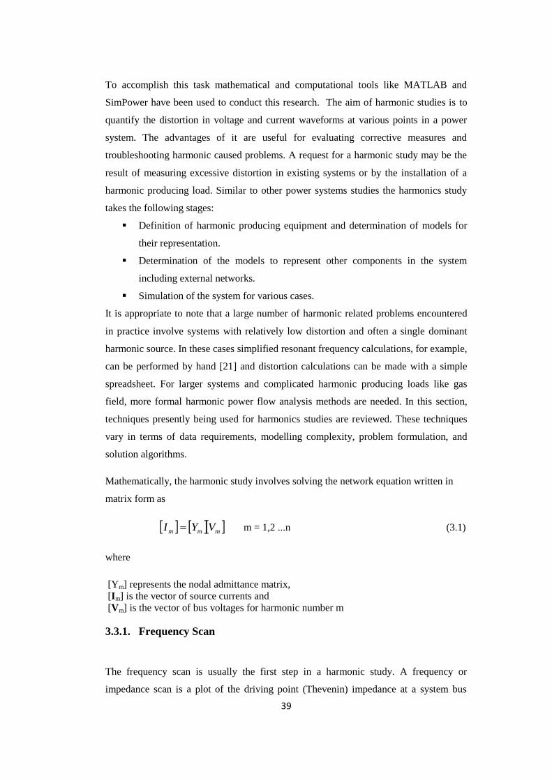
39
To accomplish this task mathematical and computational tools like MATLAB and
SimPower have been used to conduct this research. The aim of harmonic studies is to
quantify the distortion in voltage and current waveforms at various points in a power
system. The advantages of it are useful for evaluating corrective measures and
troubleshooting harmonic caused problems. A request for a harmonic study may be the
result of measuring excessive distortion in existing systems or by the installation of a
harmonic producing load. Similar to other power systems studies the harmonics study
takes the following stages:
Definition of harmonic producing equipment and determination of models for
their representation.
Determination of the models to represent other components in the system
including external networks.
Simulation of the system for various cases.
It is appropriate to note that a large number of harmonic related problems encountered
in practice involve systems with relatively low distortion and often a single dominant
harmonic source. In these cases simplified resonant frequency calculations, for example,
can be performed by hand [21] and distortion calculations can be made with a simple
spreadsheet. For larger systems and complicated harmonic producing loads like gas
field, more formal harmonic power flow analysis methods are needed. In this section,
techniques presently being used for harmonics studies are reviewed. These techniques
vary in terms of data requirements, modelling complexity, problem formulation, and
solution algorithms.
Mathematically, the harmonic study involves solving the network equation written in
matrix form as
mmm VYI m = 1,2 ...n (3.1)
where
[Ym] represents the nodal admittance matrix,
[Im] is the vector of source currents and
[Vm] is the vector of bus voltages for harmonic number m
3.3.1. Frequency Scan
The frequency scan is usually the first step in a harmonic study. A frequency or
impedance scan is a plot of the driving point (Thevenin) impedance at a system bus
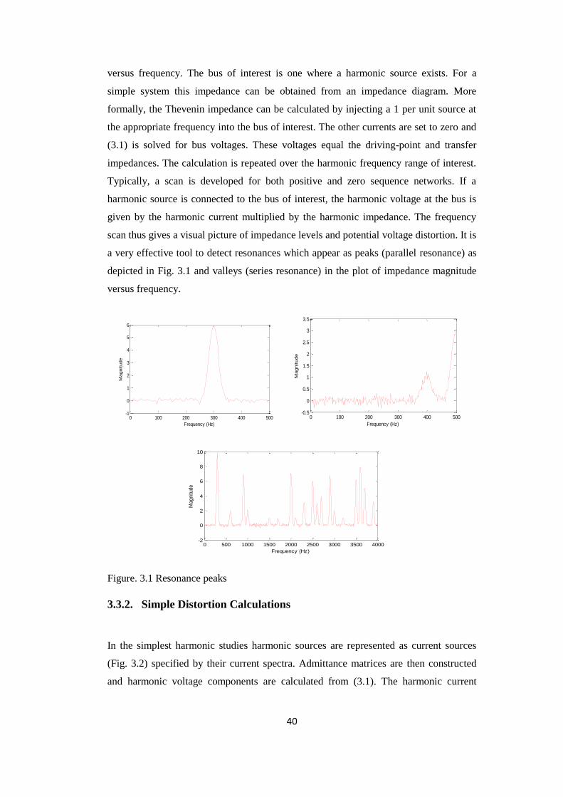
40
versus frequency. The bus of interest is one where a harmonic source exists. For a
simple system this impedance can be obtained from an impedance diagram. More
formally, the Thevenin impedance can be calculated by injecting a 1 per unit source at
the appropriate frequency into the bus of interest. The other currents are set to zero and
(3.1) is solved for bus voltages. These voltages equal the driving-point and transfer
impedances. The calculation is repeated over the harmonic frequency range of interest.
Typically, a scan is developed for both positive and zero sequence networks. If a
harmonic source is connected to the bus of interest, the harmonic voltage at the bus is
given by the harmonic current multiplied by the harmonic impedance. The frequency
scan thus gives a visual picture of impedance levels and potential voltage distortion. It is
a very effective tool to detect resonances which appear as peaks (parallel resonance) as
depicted in Fig. 3.1 and valleys (series resonance) in the plot of impedance magnitude
versus frequency.
0 100 200 300 400 500-1
0
1
2
3
4
5
6
Frequency (Hz)
Magnitude
0 100 200 300 400 500-0.5
0
0.5
1
1.5
2
2.5
3
3.5
Frequency (Hz)
Magnitude
0 500 1000 1500 2000 2500 3000 3500 4000-2
0
2
4
6
8
10
Frequency (Hz)
Magnitude
Figure. 3.1 Resonance peaks
3.3.2. Simple Distortion Calculations
In the simplest harmonic studies harmonic sources are represented as current sources
(Fig. 3.2) specified by their current spectra. Admittance matrices are then constructed
and harmonic voltage components are calculated from (3.1). The harmonic current
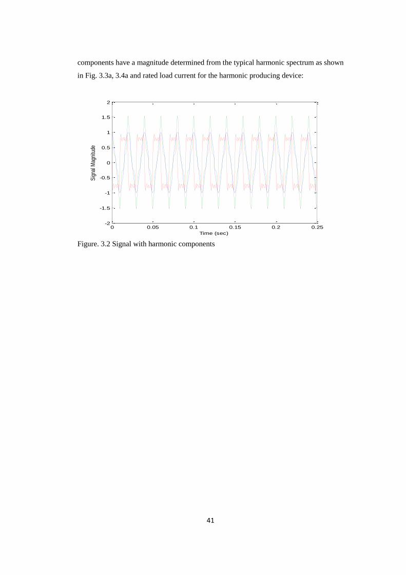
41
components have a magnitude determined from the typical harmonic spectrum as shown
in Fig. 3.3a, 3.4a and rated load current for the harmonic producing device:
0 0.05 0.1 0.15 0.2 0.25-2
-1.5
-1
-0.5
0
0.5
1
1.5
2
Time (sec)
Sig
nal M
agni
tude
Figure. 3.2 Signal with harmonic components

42
0 5 10 15 20 25 300
0.5
1
1.5
Harmonic SpectrumA
mplitu
de
0.05 0.1 0.15 0.2 0.25 0.3 0.35 0.4 0.45 0.5
-1
0
1
Time (sec)
Am
plitu
de
max.har.=29
Figure. 3.3 (a) Typical harmonic spectrum and (b) signal
0 5 10 15 20 25 300
0.5
1
Harmonic Spectrum
Am
plitu
de
0.05 0.1 0.15 0.2 0.25 0.3 0.35 0.4 0.45 0.5
-1
0
1
Time (sec)
Am
plitu
de
max.har.=29
Figure. 3.4 (a) Typical harmonic spectrum and (b) signal
spectrumspectrumnratedn IIII 1/ (3.2)
where n is the harmonic order and the subscript ‘spectrum’ indicates the typical
harmonic spectrum of the element.
b
a
a
b

43
For the multiple harmonic source cases it is important to also model the phase angle of
harmonics. A fundamental frequency power-flow solution is needed, because the
harmonic phase angles are functions of the fundamental frequency phase angle as
follows:
spectrumspectrumnn n 11 (3.3)
where θ1 is the phase angle of the harmonic source current at the fundamental
frequency.
θn-spectrum is the phase angle of the n-th harmonic current spectrum.
Depending on the phase angles used, the effects of multiple harmonic sources can either
add or cancel. Ignoring phase relationships may, therefore, lead to worst possible
outcome case or optimistic results.
3.3.3. Harmonic Power Flow Methods
The simple distortion issue discussed above is the basis for most harmonic study
software and is useful in many practical cases. The main drawback of the method is the
use of ‘typical’ spectra. This prevents inclusion of non-typical operating conditions.
Such conditions include partial loading of harmonic-producing devices, excessive
distortion and unbalance. To explore such conditions the researcher must develop
typical spectra for each condition when using the simplified method such as Newton-
Raphson. The negative effects have prompted the development of advanced harmonic
analysis methods. The goal is to model the physical aspects of harmonic generation
from the device as a function of actual system conditions.
The general idea is to create a model for the harmonic producing device in the form
0,,...,,,..., 2121 CIIIVVVF nn (3.4)
Where V1, V2, ...,Vn are harmonic voltage components, I1,I2, ...,In are corresponding
harmonic current components and C represents multiple operating and design
parameters. Equation (3.4) allows the derivation of harmonic currents from voltages and
includes power flow constraints.

44
A popular method is the so called “harmonic iteration method” [22,23]. Equation (3.4)
is first solved using an estimated supply voltage. The resulting current spectrum is used
in (3.1) to calculate the supply voltage. This iterative process is repeated until
convergence is achieved. Reliable convergence is achieved although difficulties may
occur when sharp resonances exist. Convergence can be improved by including a
linearized model in (3.1). A particular advantage of this “fast decoupled” approach is
adopted; the device model in the form of (3.4) can be in a closed form, a time-domain
model, or in any other suitable form.
Alternatively, (3.1) and (3.4) can be solved simultaneously using Newton-Raphson type
algorithms. This method requires that device models should be available in closed form
wherein derivatives can be efficiently computed [24]. Both (3.1) and (3.4) are cast in a
multiphase framework [22][25]. The focus of this approach can have several
advantages. Foremost is the modelling of zero sequence current flow. Another is the
capability of solving non-characteristic harmonics.
It should be reiterated that harmonic studies can be performed in the time domain, by
running a time-domain simulation until a steady state is reached. The challenge is first
to identify that a steady-state has indeed been achieved. Secondly, in lightly damped
systems techniques are needed to obtain the steady-state conditions within a reasonable
amount of computation time [25][26].
3.4. Modelling of Harmonic Source
The most common model for harmonic studies is the one of harmonic current source,
specified by its magnitude and phase spectrum [27]. The phase is usually defined with
respect to the fundamental component of the terminal voltage. The data can be obtained
from an idealized theoretical model or from actual measurements. In many cases, the
measured waveforms bring more realistic representation of the harmonic sources to be
modelled. This is particularly the case if noninteger harmonics are present. When a
system contains a single dominant source of harmonics the phase spectrum is not
important as shown in Fig 3.5.

45
0 500 1000 1500 2000 2500 3000 3500 4000-200
-100
0
100
200Phase spectrum
Frequency[Hz]
Phase [
degre
es]
0 500 1000 1500 2000 2500 3000 3500 40000
0.2
0.4
0.6
0.8
1Magnitude spectrum
Frequency[Hz]
Magnitude
Figure 3.5. A single dominant source of harmonics (a) the phase signal (b) magnitude
spectrum
However, phase angles must be represented when multiple sources are present. A
common method is to modify the phase spectrum according to the phase angle of the
fundamental frequency voltage seen by the load. Ignoring phase angles does not always
result in the ‘worst scenarios’.
If voltage distortion is significant or unbalanced, a more detailed model becomes
necessary. There are three basic approaches that can be taken to derive detailed models:
Develop analytical formulas for the Fourier series as a function of terminal
voltage and operating parameters for the device.
Develop analytical models for device operation and solve for device current
waveform by a suitable iterative method.
Solve for device steady state current waveform using time domain simulation.
In the analysis of distribution systems one may deal with a harmonic source that is an
aggregate of many sources. Such a source can be modelled by measuring the aggregate
a
b

46
spectrum or developing a current source type model analytically based on load
composition data [28].
3.4.1. Power Electronics Converters
Examples of power electronics devices are adjustable speed drives, VSC-HVDC
stations, static VAR compensator (SVC), the thyristor-controlled series compensator
(TCSC), the static synchronous compensator (STATCOM) and the unified power flow
controller (UPFC) [29]. Harmonic current source models are commonly used to
represent these devices. The phase angles of the current sources are functions of the
supply voltage phase angle. They must be modelled adequately for harmonic analysis
involving more than one source. The devices are sensitive to supply voltage unbalance.
For large power electronics devices such as HVDC terminals and transmission level
VSCs, detailed three-phase models may be needed. Factors such as firing–angle
dependent harmonic generation and supply voltage unbalance are taken into account in
the model [30]. These studies normally scan through various possible device operating
conditions and filter performance.
3.4.2. VSC-HVDC Stations
The conventional HVDC transmission systems use line commutated current source
converters (CSC) [31]. In these converters each valve consists of a number of thyristors
connected in series. The turn-on of the thyristor is controlled by the gate signal while
the turn-off occurs at the zero crossing of the AC current which is determined by the AC
network voltage (i.e. line commutation), where both the sending end and receiving end
of the HVDC system absorb reactive power from the AC systems. Hence, the HVDC
system requires an AC system at least at one end to have an AC voltage to commutate.
The reactive power requirement is a constraint for HVDC stations connecting to a weak
AC system or small island AC network [32].
An alternative for HVDC applications is the use of VSCs, which eliminate the reactive
power compensation requirements and this approach are used this studies [33]. Having
this advantage, the VSC-HVDC technology opens a wide range of applications

47
[34][35]. Some of the most interesting applications and possibilities of VSC-HVDC are
as follows:
Multi-terminal DC grid.
Connection of wind farms to the main grid.
Utilizing existing right-of way.
Other application of the VSC-HVDC stations is the point-to-point tie station, where no
DC line or cable exists. The VSC-HVDC point-to-point station comprises two VSCs
sharing a DC capacitor in the DC link [36]. The HVDC-VSCs are not only capable of
controlling the power flow, but can supply reactive power and provide independent
dynamic voltage control at its two terminals.
3.5. Harmonic Producing Loads
Nonlinear loads inject harmonic currents or harmonic voltages into the distribution
network, even when fed by a sinusoidal voltage or current waveform. Nonlinear loads
can be broadly divided into two categories;
Harmonic current source type loads
Harmonic voltage source type loads
Figure 3.6. Norton equivalent circuits for harmonic current source type load
(a) Current Source nonlinear load (b) Per-phase equivalent circuit of thyristor rectifier
Harmonic
Source
IL Vs
-
+
Ys
Zs
Harmonic Source
VT
L
o
a
d
AC Source
Vs
Nonlinear Load

48
Thyristor controlled loads such as those used for dc drives; current-source inverters
(CSIs), etc. constitute harmonic current source type loads. These loads produce
harmonic currents on the ac supply side of the rectifier.
Therefore, harmonic current source type loads can be modelled by a simple current
source or Norton equivalent circuit as shown in Fig. 3.6.
In contrast, VSC with dc side capacitors constitute harmonic voltage source type loads.
These loads produce voltages on the dc side of the inverter to operate.
These simple Norton and Thevenin equivalent circuit models are however to be used
with caution, since under special conditions such as resonance conditions, they do not
accurately model the harmonic sources. Similarly, harmonic voltage source type loads
can be modelled by simple voltage source or Thevenin equivalent circuit as shown in
Fig. 3.7.
Figure 3.7. Thevenin equivalent circuit for harmonic voltage source type load
3.6. Methods for Determining Sources of Harmonic Distortion
Harmonic distortions have become an important concern for oil and gas explorations
and production companies. Two basic approaches have been proposed for controlling
the amount of harmonic pollution present in a distribution system. The first scheme
involves the establishment of limits on the amount of harmonic currents and voltages
generated by platforms and utilities [37-38]. A second scheme, based on the power
factor management practice, aims at charging harmonic generators to an amount
commensurate with their harmonic pollution level when the limits are exceeded. A great
deal of work in this area was described by [39] and [40].
The challenge in the implementation of the above schemes is the need to separate the
harmonic generated by the customer equipment from that of the supply system.
(a) Diode rectifier for ac drives, electronic
equipment, etc
(b) Per-phase equivalent circuit of diode rectifier
L
o
a
d
Zs
Harmonic Source
VT
AC Source
Vs
Nonlinear Load
iL
Harmonic
Source
VL Vs
-
+
Zs

49
3.6.1. Harmonic Power Flow Direction Method
The harmonic source detection is the power direction method which checks the
direction of harmonic power flow [41][42]. The side that generates harmonic power is
considered to contain the dominant harmonic source or to have a larger contribution to
the harmonic distortions observed at the measurement point. This can be analysed using
a harmonic Norton equivalent circuit of a utility customer interface as shown in Fig. 3.8.
Figure. 3.8. Norton equivalent circuit of a utility customer interface
where
I customer the disturbance sources are the customer harmonic source
I utility. the utility harmonic source
Z u and Z c are the harmonic impedances of the respective parties.
The circuit is applicable to different harmonic frequencies. The task of harmonic source
detection is to determine which side contributes more to the harmonic distortion at the
PCC, subject to the constraint that measurements can only be taken at the PCC. To
determine which side causes more harmonic distortion at the harmonic order h, the
power direction method first measures voltage and current at the PCC and then
calculates the following harmonic power index:
PCCPCC IVP (3.5)
where Vpcc and Ipcc are the harmonic voltage and current at the PCC for a particular
harmonic number. The direction of P is defined as positive when it flows from the U
side to the C side. Conclusions of the power direction method are the following:
If P > 0 , the U side causes more hth harmonic distortion
If P < 0 , the C side causes more hth harmonic distortion
Iutility
Icustomer
Ipcc
Zc Zu Vpcc

50
If there is no change in the utility and customer harmonic impedances, then the PCC
current flow variation is affected by Iu and Ic only. It is common practice in industry that
utilities provide Zu information to customers when a plant is built or major changes are
made to the utility systems. The data is used for harmonic filter design and for harmonic
limit compliance verification. Zu is normally referred to as the contract impedance and
should therefore be known [43]. The same applies to Zc since a harmonic limit
compliance check also needs this impedance. An important assumption for this analysis
is that both Zu and Zc are known to be accurate.
The explanation of harmonic power flow direction is theoretically equivalent to
examining the magnitude of Iu Z u and Ic Z c .
Figure. 3.9. Thevenin equivalent circuit of a utility customer interface
If Iu Zu is greater than Ic Zc, then it can be shown that the utility side source contributes
more to PCC I , and vice versa. Therefore, the circuit of Fig. 3.8 is transformed into the
Thevenin equivalent circuit as shown in Fig. 3.9.
In this figure, Z = Zu + Zc , Eu = Iu Zu , and Ec = Ic Zc . The phase angle of Eu is set to
zero and that of Ec is denoted as δ. The harmonic source detection problem is to identify
which voltage source Ec or Eu has a higher magnitude [43].
However, following the classic power angle equation, if Z = jX , then the active power
flowing into Eu is:
sincosX
EEIEP cu
u (3.6)
The significance of this equation is that the direction of active power is a function of δ
instead of the magnitudes of the voltage sources. As a result, the active power direction-
based harmonic source detection method may not be accurate, as it cannot reveal the
difference between the magnitudes of the two sources [44].
I
0uE
jQP
cE
Zc Zu
Pcc

51
It is common knowledge to power engineers that the phase angles of bus voltages
mainly affect the flow of active power while the magnitudes of bus voltages mainly
affect the flow of reactive power. On examining the reactive power flowing into Eu,
uc
u
u EEX
EIEQ cossin (3.7)
The above equation shows that the direction of reactive power is indeed related to the
voltage magnitudes. Hence the direction of reactive power could indicate the relative
magnitudes of two harmonic sources. However, even the reactive power is not a
conclusive indicator of the source of harmonics. The reason is, for instance, that reactive
power can still flow from the utility side to the customer side if Ec > Eu. The direction
of power flow is always dependent on δ and has to be considered while carrying out any
measurements [43].
3.6.2. Load Impedance Variation Method
In [44], the paper focus on finding the relationship between the distorted voltage
waveform, the distorted current waveform, and the parameters that relates these
waveforms, i.e. the load parameters (R and L). Monitoring the load parameter (R & L
values) variations under the influence of harmonics plays an important role in
determining the origin of harmonic distortion and evaluating the load nonlinearity. The
load with higher R and L value variations contains more nonlinear elements and
produces larger harmonic magnitudes. A sinusoidal voltage applied to a linear load
yields a sinusoidal current. On the other hand, a distorted current waveform will result if
a sinusoidal voltage is applied to a nonlinear load. Likewise, if a sinusoidal current is
injected through nonlinear impedance, the voltage across that element will be distorted.
Thus, nonlinear loads indicate distorted voltage and/or distorted current waveforms but
the opposite is not true.
A load with a distorted current or voltage waveform is not necessarily nonlinear. So,
considering only the distorted current and voltage waveforms, it is not possible to
pronounce the source of the harmonics. It is mainly dependent on the behaviour of the
load impedance. Thus, the first step is to find a simple way to monitor the load pattern
under the influence of harmonics. Generally for a RL load,
dt
titLdtitRtv
)()()()()(
(3.8)
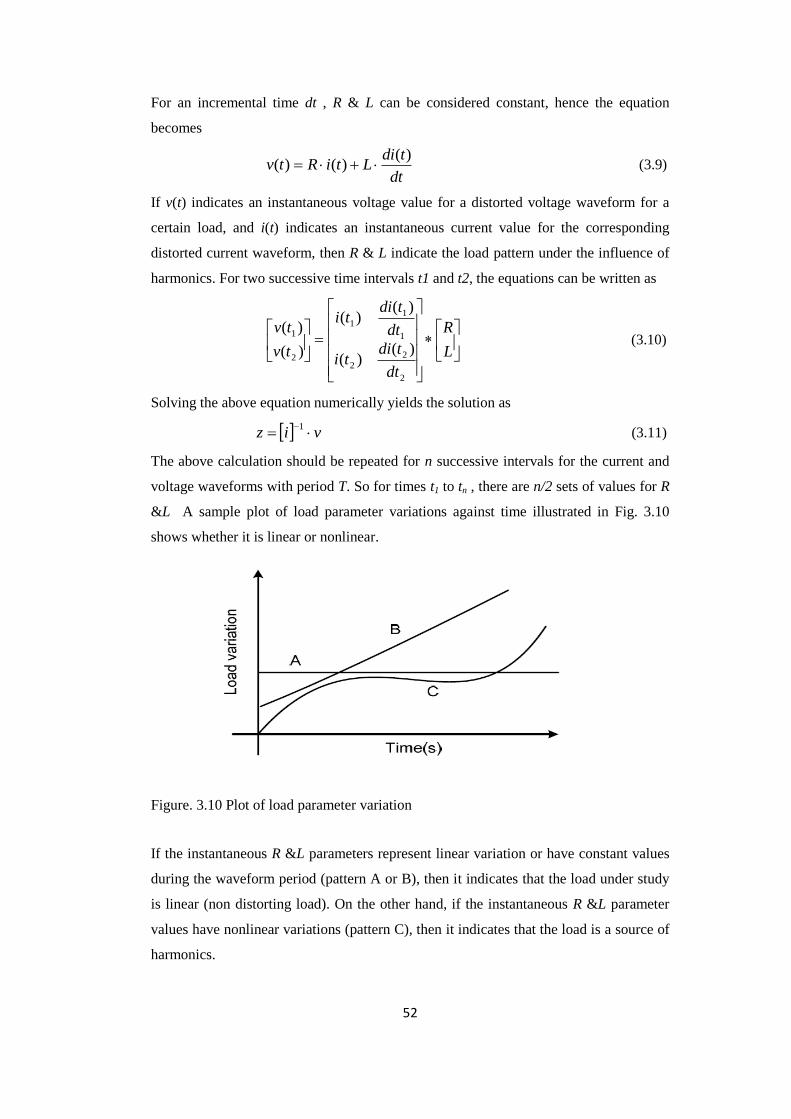
52
For an incremental time dt , R & L can be considered constant, hence the equation
becomes
dt
tdiLtiRtv
)()()( (3.9)
If v(t) indicates an instantaneous voltage value for a distorted voltage waveform for a
certain load, and i(t) indicates an instantaneous current value for the corresponding
distorted current waveform, then R & L indicate the load pattern under the influence of
harmonics. For two successive time intervals t1 and t2, the equations can be written as
L
R
dt
tditi
dt
tditi
tv
tv
2
22
1
11
2
1
)()(
)()(
)(
)( (3.10)
Solving the above equation numerically yields the solution as
viz 1
(3.11)
The above calculation should be repeated for n successive intervals for the current and
voltage waveforms with period T. So for times t1 to tn , there are n/2 sets of values for R
&L A sample plot of load parameter variations against time illustrated in Fig. 3.10
shows whether it is linear or nonlinear.
Figure. 3.10 Plot of load parameter variation
If the instantaneous R &L parameters represent linear variation or have constant values
during the waveform period (pattern A or B), then it indicates that the load under study
is linear (non distorting load). On the other hand, if the instantaneous R &L parameter
values have nonlinear variations (pattern C), then it indicates that the load is a source of
harmonics.

53
This mathematical approach can be applied to any set of measured values of v and i, for
any load category. From the plots of load parameter variation versus time, it can be
predicted whether the load that possesses sharp variations in its R &L parameters would
be the higher harmonic producing load.
3.7. Total Harmonic Voltage Distortion (VTHD) and Current Distortion(ITHD)
The voltage total harmonic distortion (VTHD) is dependent on the magnitude of each
harmonic current at its specific harmonic frequency acting upon the source impedance
and other individual circuit impedances to produce individual harmonic voltage drops.
These are summed and compared with the fundamental voltage to obtain, in percentage
terms, the VTHD. The resultant voltage distortion, unless resonance is present in the
system, tends to decrease further in its measured values from the harmonic-producing
load. It is usually highest nearer to the harmonic load and progressively reduces the
nearer to the source it is measured, due to the effect of cables, transformers and other
impedances, and to a degree, the amount of linear load (such as induction motors),
which tends to act as a “harmonic sink” (i.e., it absorbs harmonic current) in the circuit.
The higher the magnitude of harmonic current, the higher the voltage distortion for
given impedance.
In nonlinear loads, the magnitude of the characteristic harmonic currents is normally
proportional to the load demand. At rated load, the harmonic current levels tend to be at
the highest levels, except under resonant conditions where specific harmonic currents at
the resonant frequency can have significantly higher values. The effect of loading,
therefore, will affect the percentage current total harmonic distortion (ITHD).
3.8. Total Harmonic Distortion
The most commonly used measure for harmonics is total harmonic distortion (THD),
also known as the distortion factor. It is applied to both voltage and current. If DC is
ignored, then the THD for a current waveform is defined as:
1
2
2
1
2
2
)(
2
2
I
I
I
I
THDk
kk
k
I
(3.12)
THD and RMS values are directly linked as shown below:

54
2
, 1 IrmsIrms THDII (3.13)
Line losses always increase when harmonics are present because these losses are
proportional to the square of the rms current. Sometimes they increase more rapidly due
to the resistive skin effect.
The total harmonic distortion quantifies the thermal effect of all the harmonics. THD
applies to both current and voltage and is defined as the rms value of harmonics divided
by the rms value of the fundamental, and then multiplied by 100%. THD of current
varies from a few percent to more than 100%. THD of voltage is usually less than 5%.
Voltage THDs below 5% are widely considered acceptable, but values above 10% are
definitely and will cause problems for sensitive equipment and loads.
3.9. Harmonic Current Magnitude and its Effect on Voltage Distortion
It should be re-emphasized that it is not the percentage of current total harmonic
distortion (ITHD) which is of main concern. It is the magnitude of the harmonic currents
associated with the ITHD which is of more importance, as it is the magnitudes of these
harmonic currents which interact with the system impedances to produce the individual
harmonic voltage drops at the harmonic frequencies which result in the voltage total
harmonic distortion (VTHD).
It is therefore the total harmonic voltage distortion (VTHD) which is to be the main
concern in order to minimize any adverse effects on the installed system and equipment.
Therefore, it should be the purpose of any harmonic mitigation measure employed to
reduce the total harmonic voltage distortion (VTHD) to within the necessary limits under
all operating conditions.
3.10. General Discussion on Fourier Series
Any physically realizable periodic waveform can be decomposed into a Fourier series of
DC, fundamental frequency, and harmonic terms. In sine form, the Fourier series is
1
0sin)(k
kkdc tkIIti (3.14)
where

55
Idc is the DC (i.e., average) value, Ik are peak magnitudes of the individual harmonics,
ω0 is the fundamental frequency (in radians per second), and θk are the harmonic phase
angles.
A plot of normalized harmonic amplitudes Ik/I1 is called the harmonic magnitude
spectrum, as illustrated in Figure 3.11a. The superposition of harmonic components to
create the original waveform is shown in Figure 3.11b.
The time period of the waveform is
00
12
fT
(3.15)
For a discrete/sampled signal, the frequency spectrum can be obtained as follows:
1
0
2
)()(N
n
nN
kj
enikI
(3.16)
where N is the number of samples over the period T, i(n) is the amplitude at each sample
and k = 0,1,2,....N −1. Each frequency is separated by 1/T, with the highest frequency
component at k = N/2. The highest frequency becomes k = N/2T.

56
0 0.005 0.01 0.015 0.02 0.025 0.03 0.035 0.04 0.045 0.05-1
-0.5
0
0.5
1
Time
Magnitude
3 5 7 11 13 17 19 23 250
0.2
0.4
0.6
0.8
1
Harmonic number
Magnitude
Figure. 3.11 (a) Voltage waveform (b) harmonic spectrum
The sampling frequency to avoid aliasing, also known as the Nyquist frequency, is
defined as:
)(2 nffs (3.17)
where f s is the sampling frequency and the highest frequency component contained in
the signal. For power system and harmonic studies, waveforms are normally sampled at
96 – 128 samples/cycle.
Power electronic and nonlinear loads [45][46] exhibit a special property known as half-
wave symmetry. Half-wave symmetry occurs when the positive and negative halves of a
waveform are identical but opposite, i.e.
2)(
Ttiti (3.18)
where T is the period. Waveforms with half-wave symmetry have no even-ordered
harmonics.

57
3.10.1. Harmonic Power
Harmonic powers (including the fundamental) add and subtract independently to
produce total average power. Average power is defined as:
dttitvT
P
Tt
t
avg )()(1
(3.19)
By substituting the Fourier series for voltage and current in (3.19), the average value of
all the sinusoidal terms becomes zero, leaving only the time invariant terms in the
summation, or
avgkavgavgdckrmsk
k
rmskdcdcavg PPPPdpfIVIVP ,,.....,,2,1,
1
,
(3.20)
where dpfK is the displacement power factor for harmonic k .
The harmonic power terms are mostly losses and are usually small in relation to the
total power. However, harmonic losses may sometimes be a substantial part of total
losses. According to (3.20), if there is no harmonic voltage at the terminals of a
generator, then the generator produces no harmonic power. However, due to nonlinear
loads, harmonic power does indeed exist in power systems and causes additional losses
[47].
3.11. Conclusions
This chapter has outlined a systematic harmonic mitigation of all the relevant issues
related with electric network in oil and gas circuits operating under non-sinusoidal and
sinusoidal conditions. The mitigation is based on the theory of Fourier series. The
generic apparent power has been assumed to comprise active power, reactive power and
distortion power. Utilizing the expressions of apparent power and active power, yield
the true power factor.
Realistic harmonic domain evaluations are carried out using computed software. This
method permit harmonic analysis to be performed by direct frequency domain
evaluation techniques based on self and mutual convolutions. This operation avoids the
errors introduced by numeric interpolation and aliasing due to the FFT algorithm.
58
More also, this chapter has developed from first principles the theory of harmonic
domain linearization. It has been shown that a non-linear function, when linearised
around a base operating point, leads to a harmonic Norton equivalent representation.
The admittance matrix equation contains some interesting information that leads to
derive the harmonic current and harmonic voltage of the power network. Further more,
the admittance matrix with the harmonic current and harmonic voltage of the power
network hold a strong tool for the harmonic resonance analysis.
3.12. References
[1] J. Sun, and H. Grotstollen, “Solving nonlinear equations for selective harmonic
eliminated PWM using predicted initial values”, Industrial Electronics, Control,
Instrumentation, and Automation, 1992. IEEE.
[2] J.G. James, and T.K. Saha, “An Investigation of Harmonic Content in a Remote
Mine Site,” The sixth International Power Engineering Conference (IPEC2003),
27-29 November 2003, Singapore.
[3] IEEE Recommended Practices and Requirements for Harmonic Control in
Electrical Power Systems. Approved June 18, 1992 IEEE Standards Board,
Approved January 4, 1994 American National Standards Insitute. IEEE Std 519-
1992.
[4] L.Miegeville, and P.Guerin,“Analytical Model for Assessment of the Line
Harmonic Currents Generated by a Variable Speed Drive”. European Transaction
on Electrical Power, Vol. 11. No. 1. January/February, 2001.
[5] R.M.Waggoner, “Practical Guide to Quality Power for Sensitive Electronic
Equipment, EC&M Books, Kansas 1997.
[6] Excelsys,“Regulation of Harmonics”, Application Note –AN1108
http://www.excelsys.com/wp-content/uploads/2011/09/ApplicationNoteAN1108-
RegulationofHarmonics_000.pdf
[7] R.F. Martin “Harmonic Current”, http://www.cemag.com/99ARG/Martin103.html
[8] M.Contrearas, V.Cardenas, and H. Calleja, “A Review of Solutions for Harmonic
Propagation Damping in Power Distribution Networks”, International Power
Electronics Congress, 10th IEEE
[9] A.Mansoor, and J.McKim,“An examination of the rationale for limiting harmonic
emissions from low-voltage equipment”, Electromagnetic Compatibility, 1999
IEEE
[10] G.G. Balazs, M. Horvath, I. Schmidt, and P. Kiss, “Examination of new current
control methods for modern PWM controlled AC electric locomotives”, Power
Electronics, Machines and Drives (PEMD 2012), IET.
59
[11] A. Damnjanovic, A. Islam, and A. Domijan, “Aging of distribution transformers
due to harmonics”, Harmonics and Quality of Power (ICHQP), 2010
[12] A. Damnjanovic, A. Islam, and A. Domijan, “Harmonic domain modelling of
transformer nonlinear characteristic with piece-wise approximation”, Harmonics
and Quality of Power (ICHQP), 2010
[13] C.W. Cheah, A.S. Allana, T. Lye, C.S. Chang, S.K. Panda, and S.K. Sahoo,
“Investigation of current harmonics in thruster AC drives in oil-rig platforms”,
Power Electronics and Drive Systems, Nov; 2009. PEDS.
[14] J. Portos, M.P. Reddy, and D.Eaton, “Application and advantages of PAM multi
speed motors in petroleum and chemical industries”, Petroleum and Chemical
Industry Conference (PCIC), Sept; 2010.
[15] J.R.Yacamini, L. Hu and R.A Fallaize, “Calculation of commutation spikes and
harmonics on offshore platform”, IEE Proc. Vol. 137, PIB, No. 1, pp35-48.
[16] R.Yacamini and I. D. Stewart, “Harmonic problems and calculations on offshore
Platforms,” Trans IMaee, Vol 102, pp249-259.
[17] I.D. Stewart, “Offshore Power Systems Harmonic Distortions- Problem, Nuisance
or Fact of Life”, ERA Conf Proc, Protecting Electrical Networks and Quality of
supply in a DC –Regulated Industry, pp5.2.1-5.2.11
[18] J. Rico, E. Acha, Manuel Madrigal. Dynamic Harmonic Evolution Using the
Extended Harmonic Domain. IEEE Transaction On Power Delivery, Vol. 18, No.
2, April 2003.
[19] E.Acha, A. Semlyen, N. Rajakovic. A Harmonic Domain Computational Package
for Nonlinear Problems and Its Application to Electric Arcs. IEEE
TRANSACTION ON POWER DELIVERY, Vol. 5. No 3, July, 1990.
[20] S.J. Subjak, Jr., J.S. McQuikin. “Harmonic-Causes, Effects, Measurements and
Analysis”- Update. IEEE Cement Industry Technical Conference
[21] IEEE Recommended Practices and Requirements for “Harmonic Control in
Electric Power Systems,” IEEE Standard 519-1992, IEEE, New York, 1992.
[22] W. Xu, J.R. Jose and H.W. Dommel, “A Multiphase Harmonic Load Flow
Solution Technique”, IEEE Trans on Power Systems, vol. PS-6, Feb. 1991, pp-
174-182.
[23] V. Sharma, R.J. Fleming, L. Niekamp, “An iterative Approach for Analysis of
Penetration in Power Transmission Networks,” IEEE Trans. on Power Delivery,
vol. 6, No. 4, October 1991, pp. 1698-1706.
[24] D. Xia and G.T. Heydt, "Harmonic Power Flow Studies, Part I - Formulation and
Solution, Part II -Implementation and Practical Application", IEEE Transactions
on Power Apparatus and Systems, Vol. PAS-101, June 1982, pp.1257-1270.
[25] X. Lombard, J. Mahseredjian, S. Lefebvre, C. Kieny,”Implementation of a new
Harmonic Initialization Method in EMTP,” Paper 94- SM 438-2 PWRD,IEEE
Summer Power Meeting, San Francisco, Ca., July 1994.
60
[26] A. Semlyen, A. Medina, ”Computation of the Periodic Steady State in Systems
with Nonlinear Components Using a Hybrid Time and Frequency Domain
Methodology,” Paper 95- WM 146-1 PWRS, IEEE Winter Power Meeting, New
York, NY, Jan. 1995.
[27] “Understanding Power System Harmonics”; IEEE Power Engineering Review,
November 2001 W.Mack Grady, Surya Santoso.
[28] L. William, P.E. Cotten, R. Sol and P.E. Brandell, “Analysis of Harmonic
Pollution on Power Distribution Systems”. IEEE PCIC-89-46.
[29] M. A. Kamarposhti, M. Alinezhad, H. Lesani, and N. Talebi, “Comparison of
SVC, STATCOM, TCSC, and UPFC Controllers for Static Voltage Stability
Evaluated by Continuation Power Flow Method”. 2008 IEEE Electrical Power &
Energy Conference.
[30] A. V. Jaén, E. Acha, and A. G. Expósito, “Voltage Source Converter Modeling
for Power System State Estimation: STATCOM and VSC-HVDC”. IEEE
Transactions on Power Systems, Vol. 23, No. 4, November 2008.
[31] C. Hahn, A. Semerow, M. Luther, and O. Ruhle, Member, “Generic Modeling of
a Line Commutated HVDC System for Power System Stability Studies”. 2014
IEEE
[32] H.Y.TIAN and E.K.K.SNG, “Study of Line-Commutated Thyristor Inverter under
Voltage Dips and Novel Ride-Through Solution”.IEEE.
[33] N. Gibo, K. Takenaka, M. Takasaki, and T. Hayashi, “Enhancement of Continuous
Operation Performance of HVDC with Self Commutated Converter”. IEEE
Transactions on Power Systems, Vol. 15, No. 2, May 2000.
[34] K. Friedrich, “Modern HVDC PLUS application of VSC in Modular Multilevel
Converter Topology”. 2010 IEEE.
[35] F. Wang, L. Bertling, and T. Le, “ An Overview Introduction of VSC HVDC:
State-of-art and Potential Applications in Electric Power Systems”. BOLOGNA
2011.
[36] E.M. Callavik, P. Lundberg, M.P Bahrman, and R.P. Rosenqvist, “HVDC
technologies for the future onshore and offshore grid”. 2012 Grid of the Future
Symposium.
[37] V. Sharma and A.C. Thomson, “Power system harmonic guidelines and how to
evaluate the impact of customer generated harmonics,” in Proceedings of the
IEEE Communications, Computers and Power in the Modern Environment
(WESCANEX 93), Saskatoon, Canada, pp. 797 - 800, May 1993.
[38] Electromagnetic Compatibility (EMC)-Part 3: Limits-Section 6:Assessment of
Emission Limits for Distorting Loads in MV and HV Power Systems, IEC 1000-
3-6,1996.
[39] A. McEachern, W.M. Grady, W.A. Moncrief, G.T. Heydt, and M. McGranaghan,
“Revenue and Harmonics: An evaluation of some proposed rate structures,” IEEE
Transactions on Power Delivery, Vol. 101, Issue 1, pp. 474 - 482, January 1995.

61
[40] A. Ferrero, L. Peretto, and R. Sasdelli, “Revenue metering in the presence of
distortion and unbalance: myths and reality,” in Proceedings of the International
Conference on Harmonics and Quality of Power (ICHQP98), Athens, Greece,
Vol. 1, pp. 42-47, October 14-16, 1998.
[41] W. Xu, “Power Direction Method cannot be used for Harmonic Source
Detection”. 2000 IEEE.
[42] E. Alex. Emanuel, "On the Assessment of Harmonic Pollution", IEEE Transactim
on Power Delivery. 3 Jul. l995.
[41] C. Li, W. Xu and T. Tayjasanant, “A Critical Impedance Based Method for
Identifying Harmonic Sources,” IEEE Transactions on Power Delivery, Vol. 19,
No. 2, pp. 671-678, April 2004.
[42] W. Xu and X. Liu, “An Investigation on the Validity of Power Direction Method
for Harmonic Source Determination,” IEEE Transactions on Power Delivery,
Vol. 18, No. 1, pp. 214-219, Feb. 2003.
[43] A. A. Moustafa, A. M. Moussa, and M. A. El-Gammal, “Separation of customer
and supply harmonics in electrical power distribution systems,” in Proceedings of
IEEE International Conference on Harmonics and Quality of Power(ICHQP00),
Orlando, FL, Vol. 1, pp. 208 – 213, October 1-4, 2000.
[44] N. Mohan, T.M. Undeland and W.P. Robbins, “Power Electronics: Converters,
Applications and Design,” Wiley, 3rd edition, 2002, ISBN 0-4712-2693-9.
[45] M.H. Rashid, “Power Electronics: Circuits, Devices and Applications,” Prentice
Hall, 3rd edition, 2003, ISBN 0-1310-1140-5.

62
Chapter 4
4. Harmonic Modelling of Power Line and Power Cable Systems
4.1. Introduction
Future offshore wind farms will have large power ratings and will be situated much
further offshore than current projects. An important question is how the wind energy
produced either onshore or offshore is to be transported to feed into the
onshore/offshore oil and gas production weak power system. Until now grid connection
had been considered exclusively on a per project basis. Since existing wind farms have
moderate distances to the shore of up to 25 km and power ratings up to hundreds MW,
three-phase ac transmission through underground or submarine cables at medium or
high-voltage levels has to be applied exclusively [1-2]. The high power cable
transmission challenges the realization of onsite-efficient grid connections of such wind
parks [3-7]. They introduce a problem of parallel resonance due to the interaction of
shunt capacitance of the cables with the rest of the network. As the length increases, the
shunt capacitance increases and the natural resonance frequency decreases [8].
Harmonic resonance is one of the main consequences of harmonics in power systems.
Since resonance is characterized by the inductive and the capacitive elements in the
network, changes in system impedance leads to the alteration of the resonant point.
Many harmonic related issues can be traced to this phenomenon and the tools available
to analyze the phenomenon are very limited. Frequency scan analysis is probably the
only viable method at present to identify the existence of resonance and to determine the
resonance frequency. Unfortunately the tool cannot offer additional information
required to solve the problem effectively [9-10]. Therefore, a new method has been
introduced known as modal domain analysis. In the modal domain, a number of modal
voltage waves equal to the number of active conductors is assumed to exist. In a
transmission line with more than one conductor, one of the modes will travel with a
smaller velocity and higher attenuation than the rest, and this is attributed to the ground
penetration, called the ground mode. At the sending and receiving end of the line
harmonic voltage and current excitations offer very strong tools for the cancellation of
harmonic parallel resonances.

63
4.2. Harmonic Modelling of Overhead Transmission Lines
In the most general terms, a transmission line is a system of dielectric insulating media
that is capable of guiding the electric energy transfer between a generator and a load,
irrespective (at least with a good approximation) of the bends that the line undergoes
because of installation needs. From this point of view, a one dimensional propagation
phenomenon takes place on a transmission line.
When dealing with multi-conductor transmission all the admittance matrices of the
unconnected branches of the original network components are symmetric and therefore,
the functions that represent the elements need only be evaluated for elements on or
above the leading diagonal.
The formulation of mathematical models of transmission line parameters at harmonic
frequencies is more complex than that of transmission line parameters at power
frequencies. Many factors that are normally neglected at power frequencies are needed
at harmonic frequencies [10], which include:
Long-line effects
VAR compensations
Frequency dependence
Line impedances
Line transpositions
Information at a large number of points along the line is needed for the diagnosis of
harmonic interference. The formulation of mathematical models for transmission line
parameters suitable for harmonic studies of oil and gas production field/platform are:
Evaluation of lumped parameters: The lumped parameters are generated from
the geometric configuration of the transmission line considering the ground
return and skin effects.
Evaluation of distributed parameters: Here the long-line effects are combined
with lumped parameters, to obtain exact models of transmission lines suitable
for the harmonic analysis of electrical power in the oil and gas production
industry.

64
4.2.1. Evaluation of Lumped Parameters
The definition of lumped series impedance and shunt admittance of a multi-conductor
transmission line are as follows:
Z = Ze + Zg +Zskin Ω/km (4.1)
Y = j 2πϵ0P-1
1/Ωkm (4.2)
where
ε0 = 8.854 x 10⁻⁹
F/km is the permittivity of free space
= 0h, where 0 =2πf0
f0 is the base operating frequency in Hz
h is the harmonic order
10 3/ m - Resistivity of swampy ground
100 3/ m - Resistivity of average damp earth
1000 3/ m - Resistivity of dry earth
P -Potential Coefficients
Equation (4.3) defines the impedance matrix due to the magnetic fluxes outside the
conductors, and the impedance contribution due to a lossy earth return path. The skin
effect (Zskin) is the impedance matrix due to the magnetic fluxes inside the conductors.
The potential coefficients (P) form the matrix of Maxwell’s coefficients [11].
4.2.2. Matrix of Potential Coefficients (P)
The images method used to obtain the potential coefficients are generated from the
geometrical arrangement of the conductors in the tower. The method allows the
conducting plane to be replaced by a fictitious conductor located at the mirror image of
the actual conductors. Fig. 4.1 shows when conductor l and m above ground have been
replaced by two equivalent conductors and their images located at their mirror image
[11-12].

65
Figure 4.1. Line geometry and its image
The elements of the matrix of potential coefficients (P) are given by the self-potential
coefficient pl for the lth conductor and the mutual potential coefficient Plm between the lth
and mth conductors, and are defined as follows:
lext
l
lr
yP
,
2ln (4.3)
lm
lm
lmd
DP ln (4.4)
where
22
lmlmlm yyxxD
22
lmlmlm yyxxd
rext,l is the external radius in m of the lth conductor. All variables in Figure 4.1 are given
in m. Potential coefficients depend entirely on the physical arrangement of the
conductors and need only be evaluated once.
4.2.3. Impedance Matrix of Ground Return (ZG-E)
The development of a formula based on infinite series pertaining to a current-carrying
wire above a lossy earth gave rise to the study of electromagnetic fields, propagation
characteristics and magnetic induction effects caused by power lines [13]. A satisfactory
solution to the related problem of a current carrying wire above a lossy earth was first
yl
ym
l
m
xl xm
l1
m1
Dlm
dlm
Ground level

66
brought forward by Carson in 1926. Carson’s integral was generated with the use of the
so-called Maxwell’s equations and basic concepts of circuit theory [14-15]. The solution
was given in the form of an infinite integral, which has not a closed form or analytical
answer, but it is conveniently expressed as a set of infinite series [16-18]. Carson’s
integral goes rather well with the more accurate integrals of Wedepohl or Wait, for most
conditions prevailing in power circuit problems. Heavy computational cases are
involved with the numerical solution of any of the three infinite integrals that limit their
use on an everyday application. It is only in a reduced number of conductors in close
proximity to the ground and radio frequency applications that the more accurate
approaches are used [13].
Figure 4.2. Line geometry and its image using the complex penetration approach
Based on Carson's work, in Fig. 4.2 the earth impedance can be concisely expressed as
,rJze (4.5)
where
ze ϵ eZ
= function of
,,, rrr jQPJ
rlm = lmD
22dyyD mllm
lll yD 2
Ground level
dlm
Dlm
m1
l1
xm xl
m
l
ym
yl
Complex depth
Complex depth

67
ml
llyy
darctan
o
ll 0
7104 [H/m]
f 2
is the ground’s conductivity in S/m
The P and Q terms in the preceding equations are defined by Carson as an infinite series
expressed in terms of two parameters, call them S and θ. However, the value of S and
θ differ.
Carson's solution to equation (4.5), in terms of infinite series, is
22222
2ln
81 321
1
22
14
SSSP
r
(4.6)
228222
12ln
4
1 43
21
1
44
1
S
SSQ
r
(4.7)
where 1 is the Euler's constant 1.7811 and S2,
1
2S , S4, 1
4S , 321 ,, and 4 are
infinite series, which converge quickly for most power system applications, but the
amount of required computation increases with frequency and the separation between
conductors.
For very high frequency applications and when large distances are involved the series
given in equations (4.6) and (4.7) present convergence problems.
In the late 1970s and early 1980s C. Dubanton brought forward an elegant and accurate
solution with simpler formulas aiming at a reduction in computing time, while keeping
accuracy at a reasonable level in system applications. Due to its simplicity and high
degree of accuracy for the whole frequency span for which Carson's equations are valid,
though, for a wide range of frequencies it becomes increasingly inaccurate as the angle
approaches the 2/ radians. Dubanton's formulae for the evaluation of the self and
mutual impedances of the conductors’ l and m of Fig. 4.2 are,
lext
l
EGr
pyjZ
U
,
0 2ln
2
Ω/km (4.8)
lm
mlm
EGd
pyyxxjZ
lm
22
102
ln2
Ω/km (4.9)
68
where
0 = 4π x 10-7
H/m is the permeability of free space
0
1
jp is the complex depth below the earth at which the mirroring surface
is
is the earth conductivity in S/m
- resistivity of dry earth
4.2.4. Skin Effect Impedance Matrix ZSkin
The impedance varies with frequency in a non-linear fashion, the reason being that the
current flowing in the conductor does not distribute itself uniformly over the full area
available, but it tends to flow on the surface. The effect of this behaviour is an increase
in the resistance and a decrease in the internal inductance with increasing frequency
[19]. This phenomenon is known as skin effect. This term accounts for the internal
impedance of the conductors [20-21]. Both resistance and inductance vary with
frequency in a non-linear manner and need to be computed at each particular harmonic
frequency [22]. The reasons that the non-linear variation of these parameters with
frequency have been very early recognized and are attributable mainly to the fact that
the current flowing in the conductor does not distribute itself uniformly over the full
area available, rather, it tends to flow on the surface. The overall effect is an increase in
the resistance and a decrease in its internal inductance.
In the past, extensive research both theoretical and practical has been carried out for
conductors with regular and non-regular shapes. Solid conductors, annular conductors
(tubes), rounded, squared, stranded, etc. have been investigated and different models
have been proposed. In power system applications the most successful approach has
been the one that models the power conductor as a tube. The reason being that modern
power transmission circuits utilize almost exclusively ACSR (Aluminium Conductor
Steel Reinforced) conductors and, under the assumption that a negligible amount of
current flows through the path of high resistance (the steel), the conductor can be
approximated to a tube [23-26]. The evaluation of the internal impedance of an annular
conductor with outer radio ri and inner radio rj, at a given frequency is determine by:
)()()()(
)()()()(1
2 1111
1
11
ioeoioeo
oeoioeo
o
o
cxJxNxNxJ
xJxNxNxJ
x
jZ
(4.10)
located

69
)()()()(
)()()()(1
2 1111
1
11
ioeoioeo
oeoioeo
o
o
xJxNxNxJ
xJxNxNxJ
x
jL
(4.11)
the function arguments xe and xi are obtained from
eojjx r
where r = re or r = ri
Furthermore, Jo and No represent the Bessel functions of first kind and second kind of
zero order, 1
0J and 1
0N their derivatives and c the conductivity of the conductor.
The Bessel functions and their derivatives are solved, within a specified accuracy, by
means of their associated infinite series. In some cases this is done without difficulties
because the series present convergence problems and their asymptotic expansions have
to be used. This is particularly the case at high frequencies and low ratios of thickness to
external radius, i.e. ert / or eie rrr / . An additional problem is also the time required
for them to converge.
Once again the complex penetration concept has been successfully invoked, and based
on it, an alternative solution has been proposed. The new formulation supersedes the
problems encountered by the infinite series of the Bessel functions. It is a closed form
solution, and although errors up to the 6.5 per cent exist at low frequencies, its accuracy
increases with frequency. The method appeals to the two extreme cases of the
impedance, the zero frequency solution and the infinite frequency solution. In power
systems applications a power conductor is modelled as an annular conductor (tube). The
reason behind this is that modern power transmission circuits make use exclusively of
almost ACSR (Aluminium Conductor Steel Reinforced) conductors under the
assumption that a negligible amount of current flows through the path of high resistance
(the steel) the tube concept is a realistic one [27]. The radius of the conductor is the
outer radius of the tube and the radius of the steel reinforcement is the inner radius of
the tube as shown in Figure 4.3.

70
Figure 4.3. ACSR conductors
A suitable model to determine internal impedance of an ACSR conductor using the
complex penetration concept may be established by using
ZRZUSkin
2
0 Ω/km (4.12)
where
Cllext rr
R 2
int,
2
,
0
1
(4.13)
pcr
Zclext ,2
1 (4.14)
cjpc
0
1 (4.15)
where
lrint, is the internal radius of the conductor l in m
Pc is the complex depth below the earth at which the mirroring surface is located.
c is the conductivity of the conductor in S/m
Ro is the dc resistance per unit length
This model is a closed-form formulation which overcomes difficulties experienced with
the lack of robustness of the infinite series of the Bessel functions.
rint
rext

71
4.2.5. Reduced Equivalent Matrices Zabc and Yabc
Although AC Extra High Voltage transmission lines contain a large number of
conductors, i.e. earth wires and several bundle conductors per phase, the interest of
harmonic studies is not the individual conductors but the individual phases and steps
must be taken to find reduced equivalent matrices, which should correctly account for
the original configuration while keeping essential information only, i.e. one equivalent
conductor per phase. Reduced equivalent matrices could be achieved in two different
ways:
The first method is to use the geometric mean radius (GMR), which is
frequency independent.
The second method uses matrix reduction techniques; it is frequency dependent
for the series impedance. This method requires more computation and can be
carried out using the following three steps at each frequency:
1. Matrices Z and P are set up with an order equal to the total number of
conductors plus earth wires.
2. By assuming that the voltage from line to ground is exactly the same for all the
conductors in the bundle, the transformation matrices BT and B are built up, so
that modified matrices ZRe and PRe are obtained,
ZRe = BTZB (4.16)
PRe = BTPB (4.17)
3. This is followed by a partial inversion applied to ZRe and PRe . Notice that a
number of elements equal to the number of phases are inverted, with each of the
non-inverted locations corresponding to one of the conductor per phase. The
final reduced equivalent matrices Zabc and Pabc are obtained, whose order equals
the number of phases but implicitly accounts for the original configuration.
The reduced equivalent matrix of potential coefficients Pabc is inverted and multiplied by
a constant factor to obtain the shunt admittance matrix, Yabc = j1000 2πε0 P-1
abc . The
shunt admittance parameters vary linearly with frequency [30].
72
4.3. Evaluation of Distributed Parameters
Long-line effects must be taken into account in harmonic propagation analysis as the
transmission line length increases. The nominal pi circuit model, described above, is not
valid for long-line transmission. Alternatively, the use of equivalent pi circuit model or
analogous formulations, derived from the wave propagation equation, is more robust
[29].
4.3.1. Modal Analysis at Harmonic Frequencies
The incorporation of long-line effects into multi-conductor transmission lines is not as
simple as for single phase lines, because it involves matrix rather than scalar operations.
Operations such as square roots, logarithms, circular and hyperbolic functions, etc. are
not directly defined in matrix theory. The solution adopted in power transmission line
problems has been to diagonalize the matrices, through modal analysis, and then normal
scalar operations are carried out for the decoupled matrices [30-31]. More recently, less
time demanding, yet accurate solutions have been proposed.
In general, diagonalization procedures of matrices associated with three phase
transmission lines are performed by means of iterative algorithms [32], i.e. QR
(Quadratic Residue) methods and analytical formulas exist for the special case of
configurations with centre-phase symmetry.
An alternative is a closed form approach, which is based on the solution of the cubic
equation and applies to cases of three phase transmission lines of arbitrary
configuration. However, the procedure does not solve the rather theoretical problem of
irregular eigenvalues.
4.3.2. Non-Homogeneous Lines
Series and shunt compensation as well as transpositions will often be included in
transmission systems. In such scenario each individual section of the transmission
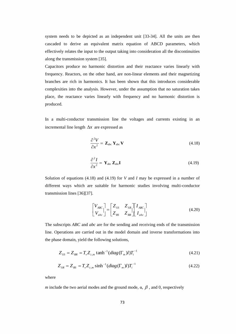
73
system needs to be depicted as an independent unit [33-34]. All the units are then
cascaded to derive an equivalent matrix equation of ABCD parameters, which
effectively relates the input to the output taking into consideration all the discontinuities
along the transmission system [35].
Capacitors produce no harmonic distortion and their reactance varies linearly with
frequency. Reactors, on the other hand, are non-linear elements and their magnetizing
branches are rich in harmonics. It has been shown that this introduces considerable
complexities into the analysis. However, under the assumption that no saturation takes
place, the reactance varies linearly with frequency and no harmonic distortion is
produced.
In a multi-conductor transmission line the voltages and currents existing in an
incremental line length x are expressed as
2
2
x
V Zabc Yabc V (4.18)
2
2
x
I Yabc ZabcI (4.19)
Solution of equations (4.18) and (4.19) for V and I may be expressed in a number of
different ways which are suitable for harmonic studies involving multi-conductor
transmission lines [36][37].
abc
ABC
RRRS
SRSS
abc
ABC
I
I
ZZ
ZZ
V
V (4.20)
The subscripts ABC and abc are for the sending and receiving ends of the transmission
line. Operations are carried out in the model domain and inverse transformations into
the phase domain, yield the following solutions,
11
, ))((tanh immcvRRSS TldiagZTZZ (4.21)
11
, ))((sinh immcvRSSR TldiagZTZZ (4.22)
where
m include the two aerial modes and the ground mode, α, , and 0, respectively
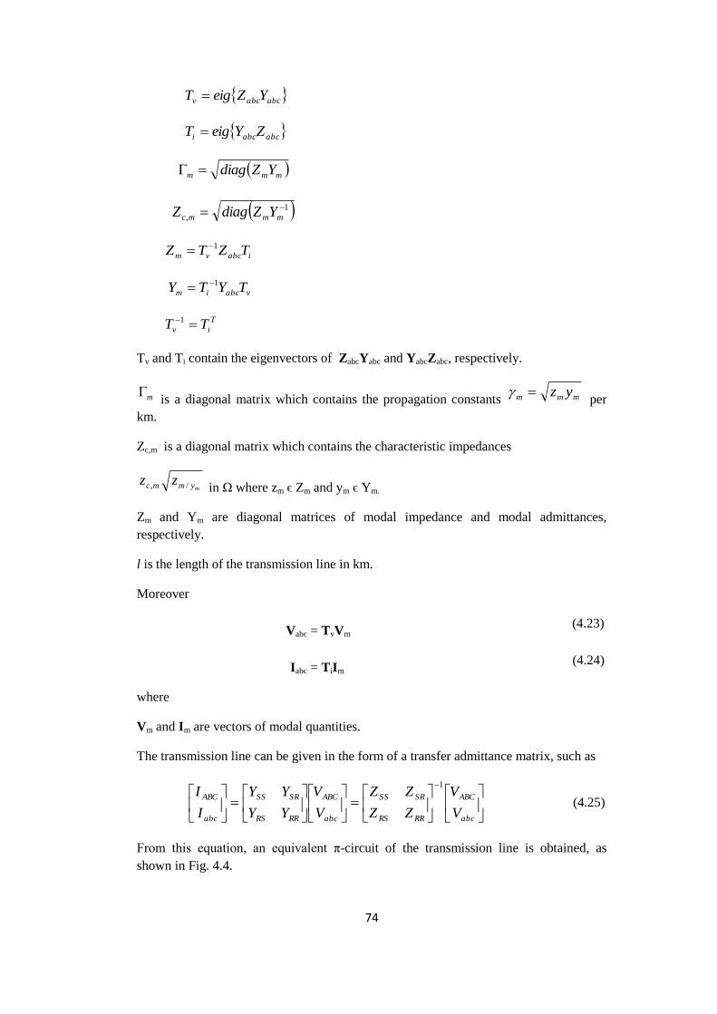
74
abcabcv YZeigT
abcabci ZYeigT
mmm YZdiag
1
,
mmmc YZdiagZ
iabcvm TZTZ 1
vabcim TYTY 1
T
iv TT 1
Tv and Ti contain the eigenvectors of ZabcYabc and YabcZabc, respectively.
m is a diagonal matrix which contains the propagation constants mmm yz per
km.
Zc,m is a diagonal matrix which contains the characteristic impedances
mymmc zz /, in Ω where zm ϵ Zm and ym ϵ Ym.
Zm and Ym are diagonal matrices of modal impedance and modal admittances,
respectively.
l is the length of the transmission line in km.
Moreover
Vabc = TvVm (4.23)
Iabc = TiIm (4.24)
where
Vm and Im are vectors of modal quantities.
The transmission line can be given in the form of a transfer admittance matrix, such as
abc
ABC
RRRS
SRSS
abc
ABC
RRRS
SRSS
abc
ABC
V
V
ZZ
ZZ
V
V
YY
YY
I
I1
(4.25)
From this equation, an equivalent π-circuit of the transmission line is obtained, as
shown in Fig. 4.4.

75
Figure 4.4. Transmission equivalent line π-circuits
The long line effects of a three-phase transmission can be incorporated using the
following method:
shuntseriesRRSS YZYY2
11 (4.26)
1 series
T
RSSR ZYY
where
11 ))(sinh( immiabcseries TldiagTZZ
abcimmishunt YTldiagTY 1
211 ))(tanh(2
Tv = eigenvectors of { Zseries Yshunt} (4.27)
Ti = eigenvectors of {Yshunt Zseries} (4.28)
z
z
z
TZT iseriesv
00
00
000
1
and
y
y
y
TYT vshunti
00
00
000
1
(4.29)
1
1
1
00
,
00
00
001
yz
yz
yz
yz
m
cm (4.30)
½Yshunt ½Yshunt
IABC VABC
Zseries VABC IABC

76
yz
yz
yz
m
00
00
0000
(4.31)
Equations (4.26)-(4.31) show that the equivalent-pi circuit model can accurately
represent the line at specific frequency. This model is a lumped parameter model and it
is good for the specific frequency of interest and particular line length. This model
includes the hyperbolic corrections with no approximations involved and is the best
model for steady-state solutions and for frequency scans. This model takes into account
the skin effect and ground return corrections.
The equivalent pi model is also multi-phase transmission line model represented in the
form of ABCD parameters matrix equation for distributed element given as
abc
abc
ABC
ABC
I
V
DC
BA
I
V
(4.32)
where
1))(cosh( vmv TldiagTA
1
, ))(sinh( immcv TldiagZTB
11
, ))(sinh( vmmci TldiagZTC
T
imi ATldiagTD 1))(cosh(
4.4. Test Case 1
The 500kV, three-phase transmission line of flat configuration shown in Figure 4.5 is
used to assess its harmonic response to voltage and current excitations. The voltage
excitation relates to a harmonic voltage excited line, specified as VS = 1 p.u. and IR = 0.
This generates the maximum voltage harmonic level necessary for design purposes.
While the current excitation is the harmonic current excited short-circuited ended line,
specified as VS = 0 and IR = 1p.u. which is more likely to be of practical interest. Both
cases are represented in Figure 4.6. It is assumed that the transmission line is 800km
long and that its operating frequency is 50 Hz.

77
Figure 4.5. Power transmission line
The following terminal conditions are assessed:
(a) (b)
Figure 4.6. Transmission line terminal conditions (a) voltage of source and open-ended
line; (b) current source and short-circuited line.
The analysis of the propagation of the voltage wave can be carried out in either the
phase domain or the modal domain. Mutual couplings exist between the phases in the
phase domain analysis and changes of voltage in one phase are a function of the
changes of voltage in the other phase. In harmonic voltage excitation at the sending end
of the line, VS, and open-ended line IR = 0, the receiving end voltage is given by
Vabc = A-1
Vs (4.33)
12.65
m
6.9m
27.5m
9m
0.46m
0.46m
VR VS
Line IR
VS VR
Line
VS = 1 ; IR = 0
VR = A-1
VS
VS = 0 ; IR = 1
VR = A-1
BIR

78
In the case of the harmonic current excitation at the receiving end, IR and short circuit
ended line at the sending end VS = 0, the receiving end voltage is given by
Vabc = A-1
BIR (4.34)
Equations (4.33) and (4.34) provide a very important conclusion. It not only simplifies
the proposed resonance mode analysis technique but also reveals the unique
characteristics of harmonic resonance.
The transmission line exhibits a resonant peak at a harmonic order which is a function
of both the length of the line and fundamental frequency,
harmonic order = kl
(4.35)
where:
is the wavelength at fundamental frequency
l is the length of the transmission line
k is equal to two when the excitation is produced by a current source and
equal to four when the excitation is produced by a voltage source.
The main technical datas of this power line are given in Table A2.1.
ABCD parameters are generated as follows:
A =
-0.7277 + 0.5690i -0.3852 + 0.6127i -0.4982 + 0.7038i
-0.4431 + 0.7160i -0.7497 + 0.4663i -0.4431 + 0.7160i
-0.4982 + 0.7038i -0.3852 + 0.6127i -0.7277 + 0.5690i
B =
1.0e+002 *
-2.8054 + 2.7093i -2.7407 + 5.1861i -2.6910 + 5.5614i
-2.7407 + 5.1861i -2.9677 + 2.8606i -2.7407 + 5.1861i
-2.6910 + 5.5614i -2.7407 + 5.1861i -2.8054 + 2.7093i

79
C =
-0.0010 - 0.0012i -0.0008 + 0.0023i -0.0009 + 0.0022i
-0.0008 + 0.0023i -0.0009 - 0.0018i -0.0008 + 0.0023i
-0.0009 + 0.0022i -0.0008 + 0.0023i -0.0010 - 0.0012i
D =
-0.7277 + 0.5690i -0.4431 + 0.7160i -0.4982 + 0.7038i
-0.3852 + 0.6127i -0.7497 + 0.4663i -0.3852 + 0.6127i
-0.4982 + 0.7038i -0.4431 + 0.7160i -0.7277 + 0.5690i
Zseries =
1.0e+002 *
-2.8054 + 2.7093i -2.7407 + 5.1861i -2.6910 + 5.5614i
-2.7407 + 5.1861i -2.9677 + 2.8606i -2.7407 + 5.1861i
-2.6910 + 5.5614i -2.7407 + 5.1861i -2.8054 + 2.7093i
Yshunt =
0.0024 - 0.0057i 0.0005 + 0.0045i 0.0011 + 0.0028i
0.0005 + 0.0045i 0.0024 - 0.0074i 0.0005 + 0.0045i
0.0011 + 0.0028i 0.0005 + 0.0045i 0.0024 - 0.0057i
4.4.1. Simulation Results
The harmonic voltage excitation at the sending end of the transmission line is fed with
fundamental frequency, 1 p.u. and the receiving end is an open circuit. In each case, the
receiving end voltages are plotted for line distance 100km, 300km, 500km and 800km
respectively.

80
0 100 200 300 400 500 600 700 800 900 10000
20
40
60
80
Voltage M
agnitude
Frequency (Hz)
phase a
phase b
phase c
Figure 4.7. Three-phase receiving end harmonic voltage excitation, 100km long
(open-circuited); for h = 1:1000; at 50 Hz.
0 100 200 300 400 500 600 700 800 900 10000
10
20
30
40
Voltage M
agnitude
Frequency (Hz)
phase a
phase b
phase c
Figure 4.8. Three-phase receiving end harmonic voltage excitation, 300km long
(open-circuited); for h = 1:1000; at 50 Hz.
0 100 200 300 400 500 600 700 800 900 10000
5
10
15
20
25
30
Voltage M
agnitude
Frequency (Hz)
phase a
phase b
phase c
Figure 4.9. Three-phase receiving end harmonic voltage excitation, 500km long
(open-circuited); for h = 1:1000; at 50 Hz
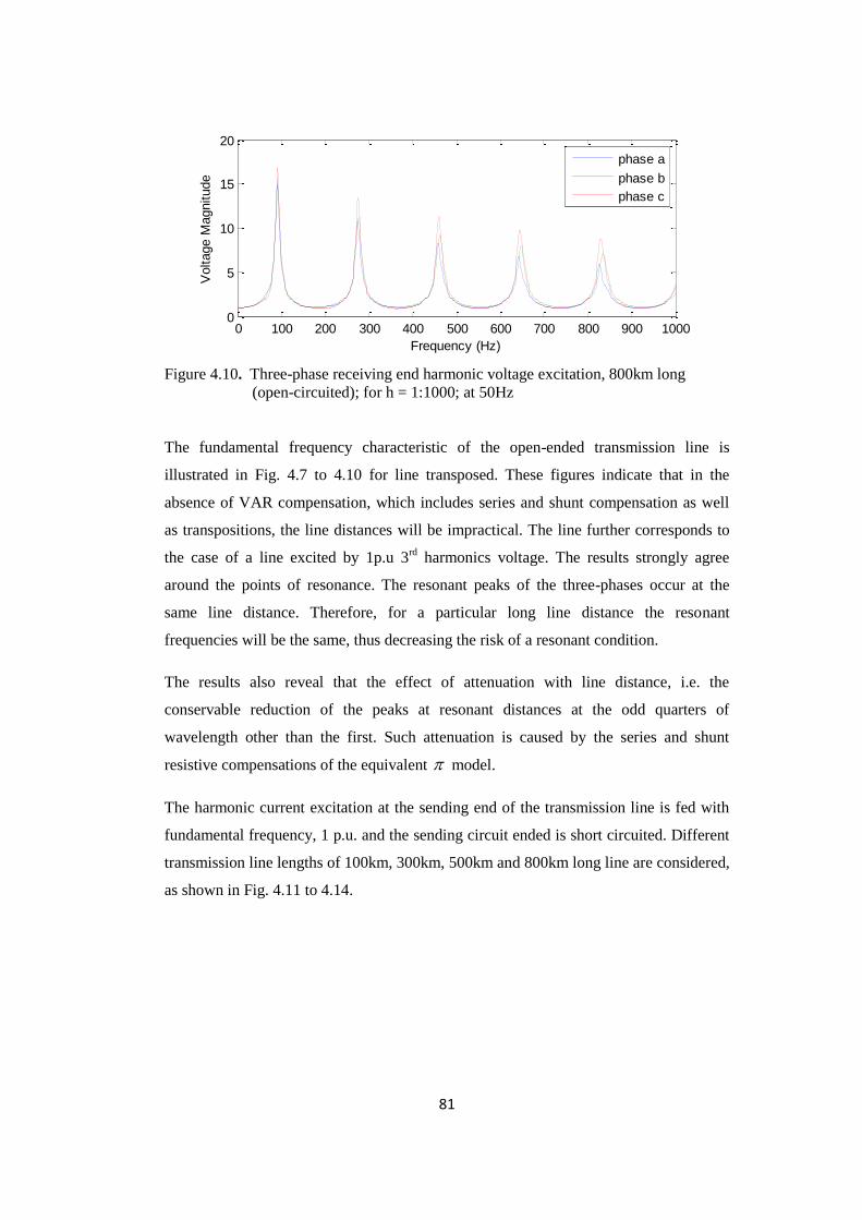
81
0 100 200 300 400 500 600 700 800 900 10000
5
10
15
20
Voltage M
agnitude
Frequency (Hz)
phase a
phase b
phase c
Figure 4.10. Three-phase receiving end harmonic voltage excitation, 800km long
(open-circuited); for h = 1:1000; at 50Hz
The fundamental frequency characteristic of the open-ended transmission line is
illustrated in Fig. 4.7 to 4.10 for line transposed. These figures indicate that in the
absence of VAR compensation, which includes series and shunt compensation as well
as transpositions, the line distances will be impractical. The line further corresponds to
the case of a line excited by 1p.u 3rd
harmonics voltage. The results strongly agree
around the points of resonance. The resonant peaks of the three-phases occur at the
same line distance. Therefore, for a particular long line distance the resonant
frequencies will be the same, thus decreasing the risk of a resonant condition.
The results also reveal that the effect of attenuation with line distance, i.e. the
conservable reduction of the peaks at resonant distances at the odd quarters of
wavelength other than the first. Such attenuation is caused by the series and shunt
resistive compensations of the equivalent model.
The harmonic current excitation at the sending end of the transmission line is fed with
fundamental frequency, 1 p.u. and the sending circuit ended is short circuited. Different
transmission line lengths of 100km, 300km, 500km and 800km long line are considered,
as shown in Fig. 4.11 to 4.14.

82
0 100 200 300 400 500 600 700 800 900 10000
5
10
15
20
25
Curr
ent
Magnitude
Frequency (Hz)
phase a
phase b
phase c
Figure 4.11. Three-phase receiving end harmonic current excitation, 100km long
(short circuited); for h = 1:1000; at 50Hz.
0 100 200 300 400 500 600 700 800 900 10000
2
4
6
8
10
Curr
ent
Magnitude
Frequency (Hz)
phase a
phase b
phase c
Figure 4.12. Three-phase receiving end harmonic current excitation, 300km long
(short circuited); for h = 1:1000; length = 300km at 50 Hz.
0 100 200 300 400 500 600 700 800 900 10000
2
4
6
8
Curr
ent
Magnitude
Frequency (Hz)
phase a
phase b
phase c
Figure 4.13. Three-phase receiving end harmonic current excitation, 500km long
(short circuited); for h = 1:1000; length = 500km at 50 Hz

83
0 100 200 300 400 500 600 700 800 900 10000
1
2
3
4
5
Curr
ent
Magnitude
Frequency (Hz)
phase a
phase b
phase c
Figure 4.14. Three-phase receiving end harmonic current excitation, 500km long
(short circuited); for h = 1:1000; length = 800km at 50Hz.
The harmonic modelling of a long transmission line feeding a static converter is as
represented in Figure 4.6b. The harmonic voltages at the point of current harmonic
injection follow the same pattern as those of the open circuit line with harmonic voltage
excitation. As shown in Figure 4.11 to 4.14 is the case of 3rd
harmonic current injection.
Voltage distortion occurs when the line length is close to a quarter wavelength, in the
case of current excited short circuited line indicates that even a 1% of harmonic current
injection can produce 3 to 4 % voltage harmonic content at the point of harmonic
current injection, which is above the levels normally granted by harmonic regulations.
The harmonic resonance increase subject the line to suffer higher levels of voltage
distortion, as shown in Figure 4.13 and Figure 4.14, the case of 5th harmonic current
injection, showing a peak voltage of about 7.0% in one of the phases of Figure 4.13.
While the case of 7th harmonic current injection, showing a peak voltage of about 4.8%
in one of the phases of Figure 4.14.
However, in these scenarios the transposed line is to reduce considerably the peaks for
the quarter wavelength distance line.
4.5. Harmonic Modelling of Underground and Subsea Cables
The offshore power generation industry has developed very rapidly in recent years.
Therefore, to model onshore and offshore electrical power systems successfully, it is
necessary to have accurate impedance models of the underground and subsea cables

84
otherwise, it is impossible to reliably predict system resonances and the effects of any
generated harmonics from power electronics converters. As the oil and gas industry
expand toward deeper sea, the cable circuits tend to increase in length. At present, cable
circuits are being employed which have lengths of the order of 100km. To develop
accurate impedance models, a good understanding of the physical phenomena that goes
into the design of the cable impedance is necessary. Also, for the power system studies,
the steady-state and harmonic generation of cables must be known. Over the years
research has been tailored to determine a suitable model for calculating the impedance
of overhead cables [38-42]. This is contrary to underground and subsea cables which
have different layers of heavy armour on the outside to give added strength both for
laying and protecting against mechanical damage. Because of the heavy armour, the
electromagnetic effects between the layers within the subsea cable need to be
considered carefully when developing impedance models. Subsea cable arrangements
and structures are diverse with inductive and capacitive element which suggests that
each cable type will generate a harmonic resonance characteristic [43-44].
A unified approach that matches the overhead transmission line is difficult for
underground and submarine cables due to their extremely complex construction and
layouts. In this thesis, a single conductor aluminium cable with a concentric lead sheath
and with insulation of XLPE is studied in detail.
Cables are principally classified based on
Their location, i.e. aerial, underground and subsea
The number of conductors, i.e. single, two and three conductor and so on
The type of insulation, i.e. oil-impregnated paper, cross linked polyethylene
(XLPE) etc.
Their protective finish, i.e. metallic (lead, aluminium) or non-metallic (braid)
The cross section of an XLPE cable is as shows in Fig. A2.4, the offshore cable
(submarine cable systems) which is made up of a core, insulation, sheath and armour,
suitable for energy transportation in upstream and midstream power systems, maybe
also suitable for underground single-core coaxial cables (SC cables). However, SC
cable with actual conductor, sheath and armour are quite often seen in the offshore
power systems [45-46]. In this thesis two high frequency cable models are investigated
and their harmonic resonance predictions are compared. The former is an approximate
model. The approximate model can give the relative contributions of the various cable
materials to the propagation characteristics of the cable. Emphasis is put on the current
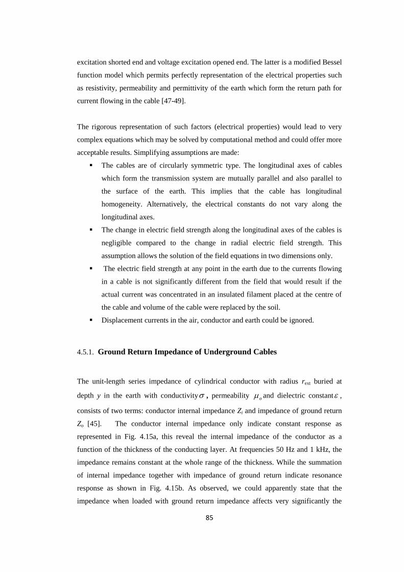
85
excitation shorted end and voltage excitation opened end. The latter is a modified Bessel
function model which permits perfectly representation of the electrical properties such
as resistivity, permeability and permittivity of the earth which form the return path for
current flowing in the cable [47-49].
The rigorous representation of such factors (electrical properties) would lead to very
complex equations which may be solved by computational method and could offer more
acceptable results. Simplifying assumptions are made:
The cables are of circularly symmetric type. The longitudinal axes of cables
which form the transmission system are mutually parallel and also parallel to
the surface of the earth. This implies that the cable has longitudinal
homogeneity. Alternatively, the electrical constants do not vary along the
longitudinal axes.
The change in electric field strength along the longitudinal axes of the cables is
negligible compared to the change in radial electric field strength. This
assumption allows the solution of the field equations in two dimensions only.
The electric field strength at any point in the earth due to the currents flowing
in a cable is not significantly different from the field that would result if the
actual current was concentrated in an insulated filament placed at the centre of
the cable and volume of the cable were replaced by the soil.
Displacement currents in the air, conductor and earth could be ignored.
4.5.1. Ground Return Impedance of Underground Cables
The unit-length series impedance of cylindrical conductor with radius rext buried at
depth y in the earth with conductivity , permeability o and dielectric constant ,
consists of two terms: conductor internal impedance Zi and impedance of ground return
Zo [45]. The conductor internal impedance only indicate constant response as
represented in Fig. 4.15a, this reveal the internal impedance of the conductor as a
function of the thickness of the conducting layer. At frequencies 50 Hz and 1 kHz, the
impedance remains constant at the whole range of the thickness. While the summation
of internal impedance together with impedance of ground return indicate resonance
response as shown in Fig. 4.15b. As observed, we could apparently state that the
impedance when loaded with ground return impedance affects very significantly the
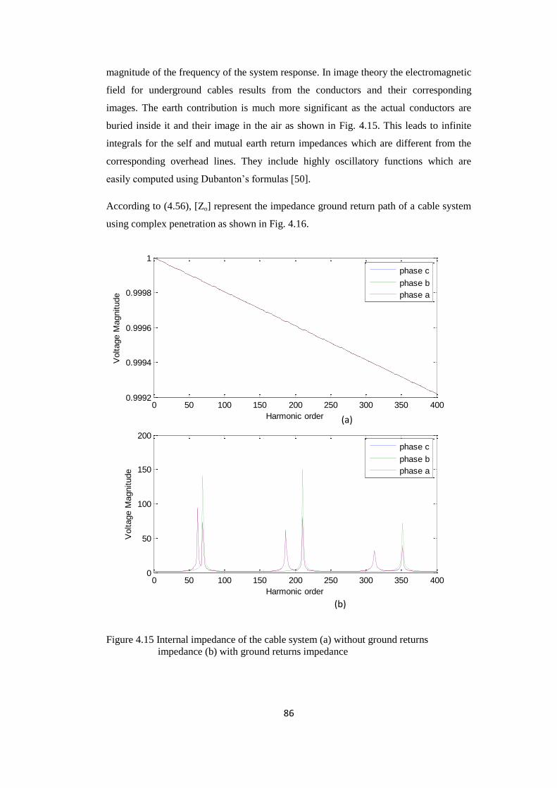
86
magnitude of the frequency of the system response. In image theory the electromagnetic
field for underground cables results from the conductors and their corresponding
images. The earth contribution is much more significant as the actual conductors are
buried inside it and their image in the air as shown in Fig. 4.15. This leads to infinite
integrals for the self and mutual earth return impedances which are different from the
corresponding overhead lines. They include highly oscillatory functions which are
easily computed using Dubanton’s formulas [50].
According to (4.56), [Zo] represent the impedance ground return path of a cable system
using complex penetration as shown in Fig. 4.16.
0 50 100 150 200 250 300 350 4000.9992
0.9994
0.9996
0.9998
1
Harmonic order
Voltage M
agnitude
phase c
phase b
phase a
0 50 100 150 200 250 300 350 4000
50
100
150
200
Harmonic order
Voltage M
agnitude
phase c
phase b
phase a
Figure 4.15 Internal impedance of the cable system (a) without ground returns
impedance (b) with ground returns impedance
(a)
(b)

87
Figure 4.16 Geometric configurations of two SC underground cables and its images
The elements of the matrix of ground return path impedance Z using Dubanton’s
equations are given by the self ground impedance
ext
lsr
jZ
1ln
2
1000 0
0 (4.36)
while the mutual ground impedance is given as
dij
jZ lm
1ln
2
1000 0
0 (4.37)
where
22
jiji yyxxdij (4.38)
yj
yi
earth
air
iii ,,
x
Dij
dij
Image of cable j
Cable i
Cable j
yie
yje
Image of cable i

88
0
1
j (4.39)
where
is the complex depth above the earth at which the mirroring surface is located.
0 = 4π x 10-7
H/m is the permeability of free space
is the conductivity of the conductor in S/m
4.6. Formation of Approximation Cable Model
Several approximations with closed-form solutions have been investigated in the issue
of overhead transmission line, but nothing promising has been investigated in the issue
of underground and submarine cables.
In this approach of complex depth concept, the infinite integral of impedance of the
conductor, and sheath taking due account of skin effect each of which is approximated
using infinite series. The current inside conductor is concentrated around the surface
due to the skin effect. It is assumed that the current density is uniform in the range
covered by the skin depth. Under this assumption, the internal impedance can be
derived by approximation method.
In the supporting routines cable parameters of harmonic study, the earth return
impedances of cables are calculated using Dubanton’s formula for a single case of two
underground conductors, which is evaluated by infinite series. The model is valid for
homogenous infinite earth, neglecting the displacement current [51-55].
Underground and submarine cables are usually divided into single or multiple core
types. For high power, three-phase AC transmission cable systems could be designed as
either a single-core cable or three single-core cables or as a single three-core cable. For
the purpose of determining the significance of the skin effect in subsea and underground
cables, single-core flat formation has been chosen for investigation in this work, where
proximity effect is insignificant.
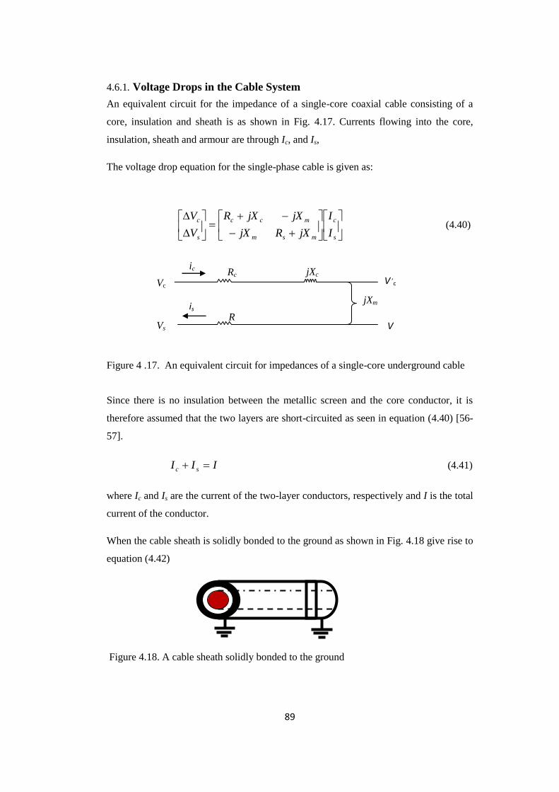
89
4.6.1. Voltage Drops in the Cable System
An equivalent circuit for the impedance of a single-core coaxial cable consisting of a
core, insulation and sheath is as shown in Fig. 4.17. Currents flowing into the core,
insulation, sheath and armour are through Ic, and Is,
The voltage drop equation for the single-phase cable is given as:
s
c
msm
mcc
s
c
I
I
jXRjX
jXjXR
V
V (4.40)
Figure 4 .17. An equivalent circuit for impedances of a single-core underground cable
Since there is no insulation between the metallic screen and the core conductor, it is
therefore assumed that the two layers are short-circuited as seen in equation (4.40) [56-
57].
III sc (4.41)
where Ic and Is are the current of the two-layer conductors, respectively and I is the total
current of the conductor.
When the cable sheath is solidly bonded to the ground as shown in Fig. 4.18 give rise to
equation (4.42)
Figure 4.18. A cable sheath solidly bonded to the ground
V ,c
jXm
jXc
R
s
Rc
is
ic
Vc
Vs V
,s

90
s
c
msm
mccC
I
I
jXRjX
jXjXRV
0 (4.42)
where c
ms
mmc
ms
mscc I
XR
XXXj
XR
XRRV
22
2
22
2
.. (4.43)
4.6.2. The Impact of Skin Effect in Power Cables System
It is an established fact that skin and proximity effects generate non-uniformed current
distribution as frequency increases, due to the magnetic field inside the conductor, the
concentration of current at the centre gradually distribute the current towards the
circumference of the conductor, thus increasing the resistance and decreasing the
internal inductance.
The impedance of the conductor and sheath considering the skin effect are determined
by the impedance of the cable conductor using complex depth concept (Zc) which is
given by [74]
2
,
2
, ccDCccc ZRjXRZ (4.44)
where 2
,cDCR is the DC resistance and is given as
cc
cDCr
R 2,
1 (4.45)
rc is the radius (m) of the conductor
cZ , is the impedance infinity of the conductor and is given as
ccc
cpr
Z2
1, (4.46)
where cp is the complex penetration and is given as
c
cj
p0
1 (4.47)
Whereas the impedance of the cable sheath (Zs)
2
,
2
, ssDCsss ZRjXRZ (4.48)
where
2
,sDCR is the DC resistance in the cable sheath , given as
si
sDCrr
R 22
0
,
1
(4.49)

91
22
0 irr is the cross-sectional area (m) of the sheath
r0 is the outer radius (m) of the sheath
ri is the inner radius (m) of the sheath
is the earth conductivity in S/m
the sZ , is the impedance infinity of the sheath , given as
ss
spr
Z 0
,2
1
(4.50)
where sp is the complex penetration and is given as
s
sj
p0
1 (4.51)
The skin effect is determined by
22
ZRZ DCskin (4.52)
The mutual reactance between the conductor and sheath is determined by
2
ln.2 0
00
i
m rr
rX
(4.53)
Due to the shielding effect of the conductor and sheath there is mutual magnetic
coupling between the outer most loop. The coupling is entirely through the earth path.
In the overhead transmission lines, the mutual reactance between phase conductors is
the sum of external mutual reactance due to the magnetic fields in the air paths and
those arising from the earth paths [51][56]. In the case of underground cable the mutual
reactance are totally contributed by the earth path only.
The self ground impedance of cable i is given as
0
0 1ln.2 r
pjZ e
ll
(4.54)
The mutual ground impedance between cables i and j in Fig. 4.17 is given as
lm
e
lmd
pjZ 1ln.
2
0
(4.55)
where ep is the complex penetration and is given as
g
ej
p0
1 (4.56)
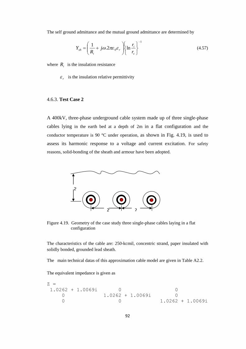
92
The self ground admittance and the mutual ground admittance are determined by
1
0 ln.2.1
c
i
r
i
shr
rj
RY (4.57)
where iR is the insulation resistance
r is the insulation relative permittivity
4.6.3. Test Case 2
A 400kV, three-phase underground cable system made up of three single-phase
cables lying in the earth bed at a depth of 2m in a flat configuration and the
conductor temperature is 90 °C under operation, as shown in Fig. 4.19, is used to
assess its harmonic response to a voltage and current excitation. For safety
reasons, solid-bonding of the sheath and armour have been adopted.
Figure 4.19. Geometry of the case study three single-phase cables laying in a flat
configuration
The characteristics of the cable are: 250-kcmil, concentric strand, paper insulated with
solidly bonded, grounded lead sheath.
The main technical datas of this approximation cable model are given in Table A2.2.
The equivalent impedance is given as
Z =
1.0262 + 1.0069i 0 0
0 1.0262 + 1.0069i 0
0 0 1.0262 + 1.0069i
2,
2,
2
93
The ground return is given as
Zground =
1.0e+002 *
0.1973 + 1.8510i 0.1932 + 0.9393i 0.1891 + 0.7694i
0.1932 + 0.9393i 0.1973 + 1.8510i 0.1932 + 0.9393i
0.1891 + 0.7694i 0.1932 + 0.9393i 0
Total impedance of the cable is given as
Zshortcable =
1.0e+002 *
0.2075 + 1.8611i 0.1932 + 0.9393i 0.1891 + 0.7694i
0.1932 + 0.9393i 0.2075 + 1.8611i 0.1932 + 0.9393i
0.1891 + 0.7694i 0.1932 + 0.9393i 0.2075 + 1.8611i
Admittance of the cable
Yshortline =
1.0e-004 *
0 + 0.9345i 0 0
0 0 + 0.9345i 0
0 0 0 + 0.9345i
The distributed parameter ABCD of the cable are given as
A =
0.1405 - 0.2768i 1.0469 - 0.2698i 0.9238 - 0.2233i
1.0469 - 0.2698i 0.2084 - 0.2443i 1.0469 - 0.2698i
0.9238 - 0.2233i 1.0469 - 0.2698i 0.1405 - 0.2768i

94
B =
57.3321 - 45.8104i 64.8186 - 40.9288i 61.2272 -11.9246i
64.8186 - 40.9288i 66.3347 - 21.9019i 64.8186 - 40.9288i
61.2272 - 11.9246i 64.8186 - 40.9288i 57.3321 - 45.8104i
C =
0.0057 - 0.0065i 0.0074 - 0.0054i 0.0068 + 0.0051i
0.0074 - 0.0054i 0.0066 + 0.0033i 0.0074 - 0.0054i
0.0068 + 0.0051i 0.0074 - 0.0054i 0.0057 - 0.0065i
D =
0.1405 - 0.2768i 1.0469 - 0.2698i 0.9238 - 0.2233i
1.0469 - 0.2698i 0.2084 - 0.2443i 1.0469 - 0.2698i
0.9238 - 0.2233i 1.0469 - 0.2698i 0.1405 - 0.2768i
4.6.4. Simulation Results
0 50 100 150 200 250 300 350 400 450 5000
10
20
30
40
Harmonic order
Voltage M
agnitude
phase c
phase b
phase a
(a)
left resonance
mode

95
0 50 100 150 200 250 300 350 4000
5
10
15
20
25
Harmonic order
Voltage M
agnitude
phase c
phase b
phase a
(b)
0 50 100 150 200 2500
5
10
15
20
Harmonic order
Voltage M
agnitude
phase c
phase b
phase a
(c)
Figure 4.20. Harmonic Impedance without voltage and current excitation
Figure 4.20 establishes the relationship between the left and right resonance mode. As
seen, the effect of including voltage or current excitation at high frequencies is desirable
to avoid the left resonance mode, which introduced high standing wave distortion as the
transmission line increases. The left resonance mode increases in peak with increase in
the line length, while the right resonance mode decreases with lower peaks.
Zseries =
57.3321 - 45.8104i 64.8186 - 40.9288i 61.2272 -11.9246i
64.8186 - 40.9288i 66.3347 - 21.9019i 64.8186 - 40.9288i
61.2272 - 11.9246i 64.8186 - 40.9288i 57.3321 - 45.8104i

96
Yshunt =
0.0163 - 0.0198i -0.0047 - 0.0614i 0.0012 + 0.0837i
-0.0047 - 0.0614i 0.0233 + 0.1145i -0.0047 - 0.0614i
0.0012 + 0.0837i -0.0047 - 0.0614i 0.0163 - 0.0198i
The skin effect is represented as
Zskin = 1.5925 + 1.1804i 1.5925 + 1.1804i 1.5925 + 1.1804i
0 50 100 150 200 250 300 350 400 450 5000
1000
2000
3000
4000
Harmonic order
Curr
ent
Magnitude
Sending end in short circuit and 1 p.u. harmonic current injection at receiving end
phase c
phase b
phase a
0 50 100 150 200 250 300 350 400 450 5000
20
40
60
80Receiving end in open circuit and 1 p.u. harmonic voltage injection at sending end
Harmonic order
Voltage M
agnitude
phase c
phase b
phase a
Figure 4. 21.1km long cable with first resonant peak appear at h = 350, NH = 500

97
0 50 100 150 200 250 300 350 4000
500
1000
1500
2000
2500
Harmonic order
Curr
ent
Magnitude
Sending end in short circuit and 1 p.u. harmonic current injection at receiving end
phase c
phase b
phase a
0 50 100 150 200 250 300 350 4000
10
20
30
40
50Receiving end in open circuit and 1 p.u. harmonic voltage injection at sending end
Harmonic order
Voltage M
agnitude
phase c
phase b
phase a
Figure 4.22 5km long cable with first resonant peak to appear at h = 70, NH = 400,
freq. = 50 Hz.
0 50 100 150 200 2500
500
1000
1500
2000
Harmonic order
Curr
ent
Magnitude
Sending end in short circuit and 1 p.u. harmonic current injection at receiving end
phase c
phase b
phase a
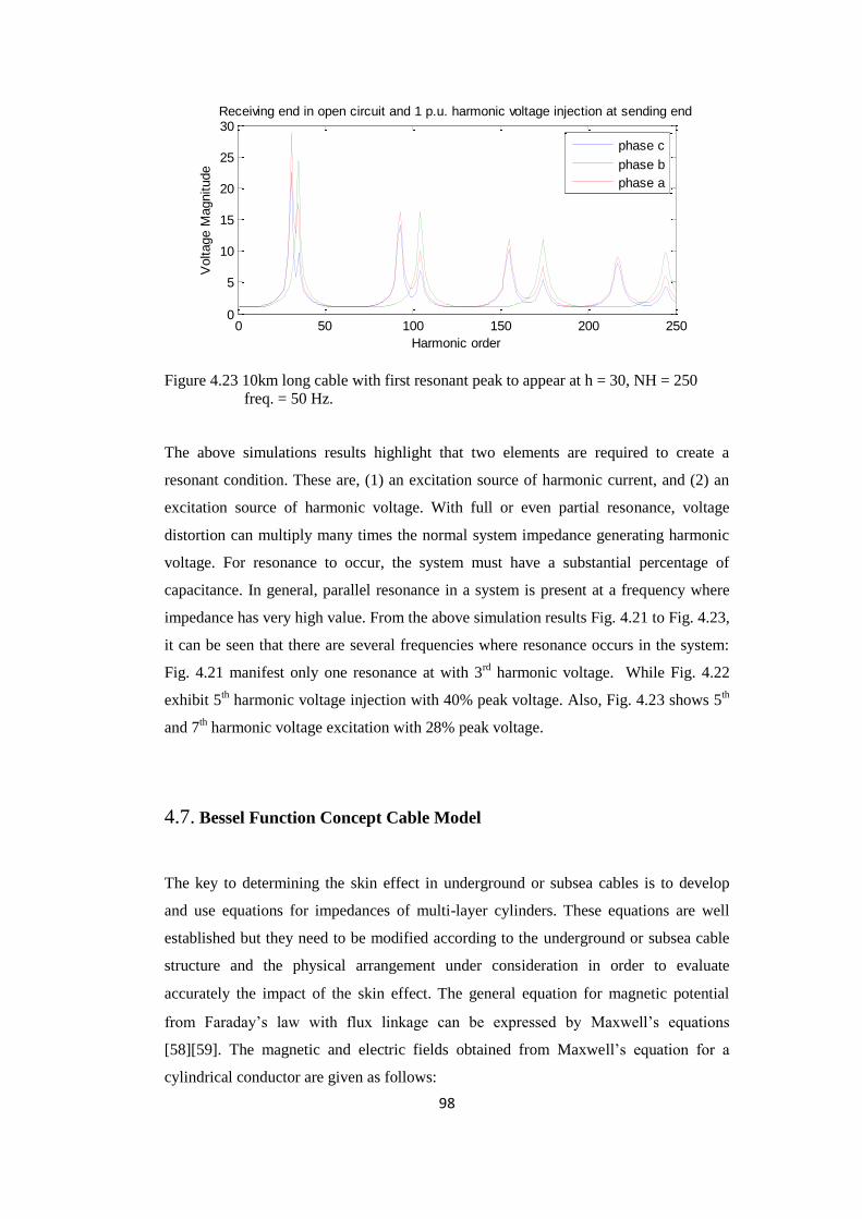
98
0 50 100 150 200 2500
5
10
15
20
25
30Receiving end in open circuit and 1 p.u. harmonic voltage injection at sending end
Harmonic order
Voltage M
agnitude
phase c
phase b
phase a
Figure 4.23 10km long cable with first resonant peak to appear at h = 30, NH = 250
freq. = 50 Hz.
The above simulations results highlight that two elements are required to create a
resonant condition. These are, (1) an excitation source of harmonic current, and (2) an
excitation source of harmonic voltage. With full or even partial resonance, voltage
distortion can multiply many times the normal system impedance generating harmonic
voltage. For resonance to occur, the system must have a substantial percentage of
capacitance. In general, parallel resonance in a system is present at a frequency where
impedance has very high value. From the above simulation results Fig. 4.21 to Fig. 4.23,
it can be seen that there are several frequencies where resonance occurs in the system:
Fig. 4.21 manifest only one resonance at with 3rd
harmonic voltage. While Fig. 4.22
exhibit 5th harmonic voltage injection with 40% peak voltage. Also, Fig. 4.23 shows 5
th
and 7th harmonic voltage excitation with 28% peak voltage.
4.7. Bessel Function Concept Cable Model
The key to determining the skin effect in underground or subsea cables is to develop
and use equations for impedances of multi-layer cylinders. These equations are well
established but they need to be modified according to the underground or subsea cable
structure and the physical arrangement under consideration in order to evaluate
accurately the impact of the skin effect. The general equation for magnetic potential
from Faraday’s law with flux linkage can be expressed by Maxwell’s equations
[58][59]. The magnetic and electric fields obtained from Maxwell’s equation for a
cylindrical conductor are given as follows:
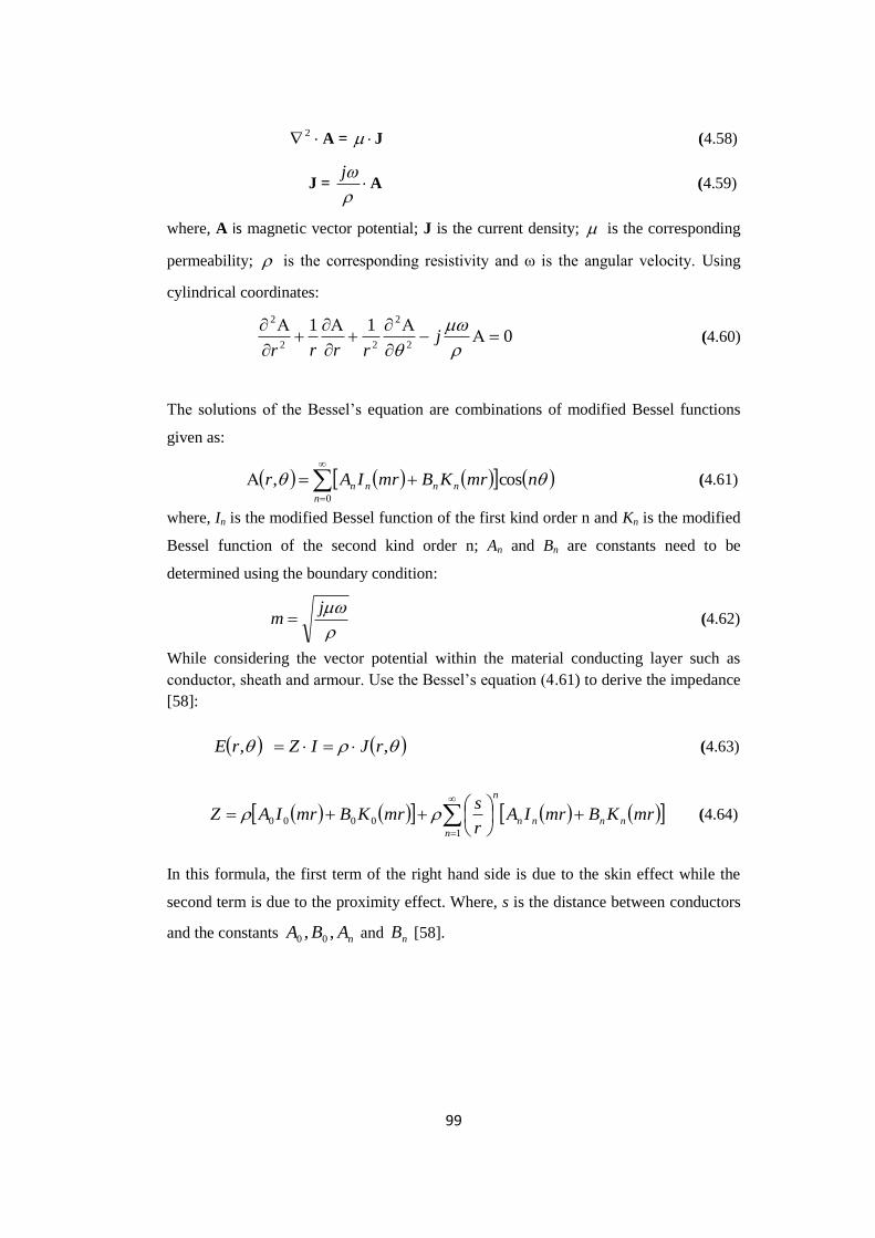
99
2A = J (4.58)
J =
jA (4.59)
where, A is magnetic vector potential; J is the current density; is the corresponding
permeability; is the corresponding resistivity and ω is the angular velocity. Using
cylindrical coordinates:
011
2
2
22
2
j
rrrr (4.60)
The solutions of the Bessel’s equation are combinations of modified Bessel functions
given as:
nmrKBmrIArn
nnnn cos,0
(4.61)
where, In is the modified Bessel function of the first kind order n and Kn is the modified
Bessel function of the second kind order n; An and Bn are constants need to be
determined using the boundary condition:
jm (4.62)
While considering the vector potential within the material conducting layer such as
conductor, sheath and armour. Use the Bessel’s equation (4.61) to derive the impedance
[58]:
,, rJIZrE (4.63)
mrKBmrIAr
smrKBmrIAZ nnnn
n
n
1
0000 (4.64)
In this formula, the first term of the right hand side is due to the skin effect while the
second term is due to the proximity effect. Where, s is the distance between conductors
and the constants nABA ,, 00 and nB [58].

100
4.7.1. The Impedance (Z) of Three-Layer Conductor
An equivalent circuit for impedance of a single-core coaxial cable consisting of a core,
sheath and armour is as shown in Fig. 4.24. Currents flowing into the core, sheath,
armour and outer medium (earth) are through Ic, Is, Ia and Ie at x.
Figure 4.24An equivalent circuit for impedances of single-core cables (SC cable)
The self-impedance diagonal matrix of an SC cable is given as
d(V)/dx = -[Z].(I) (4.65)
[Z] = [Zi] + [Zo] (4.66)
where
[Zi] is internal impedance matrix
[Zo] is earth or sea return impedance
Impedance matrix of core, sheath and armour of a cable:
[Zi] =
(4.67)
[Zo] =
(4.68)
x x + x x
Ic Ic Vc
Z11 core
V12 + V12 Z2i Z12 V12 I2
I3
Is Vs Z20
Z
2
3
Z2m
sheath
z3i I4
V23 + V23 V23
Va Ia
I5
Ie
z30 z34
z3m V34 + V34
armour
earth z0
V34
Ie
aasaca
sasscs
cacscc
ZZZ
ZZZ
ZZZ
Zij
3
2
1
00
00
00
i
i
i
Z
Z
Z
EarthEarthEarth
EarthEarthEarth
EarthEarthEarth
ZZZ
ZZZ
ZZZ

101
Also the inner and outer surface currents of the sheath and armour are I2, I3, I4, and I5 as
shown in Fig. 4.24. The voltage between the core, sheath, armour and outer medium are
V12, V23, and V34 at x and voltage at x + x are V12 + V12, V23 + V23 and V34 + V34
[45].
When the single-core cable consists of a core, sheath and armour, the self-impedance is
given by:
aajsajcaj
sajssjcsj
cajcsjccj
ij
ZZZ
ZZZ
ZZZ
Z (4.69)
where
Zccj = core self-impedance
= Zcs + Zsa + Zc4 – 2Z2m – 2Z3m
Zssj = Sheath self-impedance
= Zsaj + Zc4 -2Z3m
Zaaj = armour self-impedance
= Zc4
Zcsj= mutual impedance between the core and sheath
= Zsa + Zc4 –Z2m-2Z3m
Zcaj = mutual impedance between the core and armour
= Zc4 – Z3m
Zsaj = mutual impedance between the sheath and armour
= Zcaj
Zcs = z11 + z12 + z2i
Zsa = z20 + z23 + z3i
Zc4 = z30 + z34
4.7.2. The Component Impedance
The component impedances per unit length are given in the following equations for a
single core cable;
Z11: Internal impedance of core outer surface
11201120
12
10
11 ...1
.2
xIxKxKxIDx
sZ
(4.70)
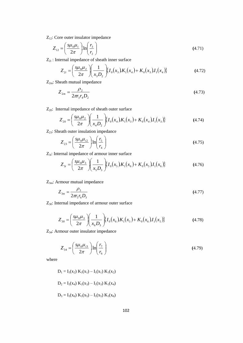
102
Z12: Core outer insulator impedance
2
310
12 ln.2 r
rsZ
(4.71)
Z2i : Internal impedance of sheath inner surface
41304130
23
20
2 ...1
.2
xIxKxKxIDx
sZ i
(4.72)
Z2m: Sheath mutual impedance
243
22
2 DrrZ m
(4.73)
Z20: Internal impedance of sheath outer surface
31403140
24
20
20 ...1
.2
xIxKxKxIDx
sZ
(4.74)
Z23: Sheath outer insulation impedance
4
520
23 ln.2 r
rsZ i
(4.75)
Z3i: Internal impedance of armour inner surface
61506150
35
30
3 ...1
.2
xIxKxKxIDx
sZ i
(4.76)
Z3m: Armour mutual impedance
365
3
32 Drr
Z m
(4.77)
Z30: Internal impedance of armour outer surface
51605160
36
30
30 ...1
.2
xIxKxKxIDx
sZ
(4.78)
Z34: Armour outer insulator impedance
6
730
34 ln.2 r
rsZ i
(4.79)
where
D1 = I1(x2) K1(x1) – I1(x1) K1(x2)
D2 = I1(x4) K1(x3) – I1(x3) K1(x4)
D3 = I1(x6) K1(x5) – I1(x5) K1(x6)

103
sx kk
n
n
mm r
0 where n = 1, 2, 3, 4, 5,..............
and m = 2, 3, 4,.................
and In(x), Kn(x) are modified Bessel function of order n.
4.7.3. The Admittance (Y) of a Cable
An equivalent circuit of a single-core coaxial cable showing the capacitive effects,
consisting of a core, sheath and armour, is as shown in Fig. 4.25 [45].
Figure 4.25 An equivalent circuit for admittances of single- core coaxial cables (SC
cable)
From Figure 4.28, we that
Ic = ycsx(Vc – Vs) + Ic + Ic
Is = ycsx(Vs – Vc) + ysax(Vs – Va) + Is + Is
Ia = ysax(Va - Vs) + ya4xVa + Ia + Ia
(4.80)
Equation 4.114 can be rewritten as
-Ic/x = ycsVc - ycsVs
-Is/x = -ycsVc + (ycs + ysa)Vs - ysaVa
-Ia/x = -ysaVs + (ysa + ya4)Va
(4.81)
If x 0
then we have the admittance matrix as,
Is
armor
sheath
core
earth Ie + Ie
Ia + Ia
Ic + Ic
Is + Is
Ie
Ia Va
Vs
Vc Ic
x x + x x
Ycs
Ysa
Ya4

104
a
s
c
a
s
c
V
V
V
yaysaysa
ysaysaycsycs
ycsycs
I
I
I
40
0
I = [Yi](V)
(4.82)
4.7.4. The Potential Coefficient (P) of a Cable
The potential coefficient is inversely related to the admittance;
aaa
aasas
aasasc
i
PPP
PPPPP
PPPPPP
P (4.83)
where
Pc = s/ycs, Ps = s/ysa, Pa = s/ya
4.8. Test Case 3
The Bessel function concept model analyzed above is applied in MATLAB software to
demonstrate the ability of identifying the resonance condition, as well as harmonic
response to a voltage and current excitation. The cable structure used is shown in Fig.
A2.4. According to design standards: BS 6622 and BS 7835, this cable can be operated
at voltages that do not exceed the voltage grade of 19/33kV single core armoured
copper conductors. The cable is 100% insulated and solidly earthed.
The main technical datas of this approximation cable model are given in Table A2.3.
Balanced three-phase voltage source = [1 -1/2-j2
3 -1/2+j
2
3]
Bessel function First Kind are generated as
J0 =
0 - 0.3058i 0 - 0.3058i 0 - 0.3058i
J1 =
2.2500 - 1.2231i 2.2500 - 1.2231i 2.2500 - 1.2231i
Modified Bessel first order are generated as
I0 =
-0.0183 + 0.0183i - 0.0183 + 0.0183i - 0.0183 + 0.0183i

105
I1 =
0 + 0.9174i 0 + 0.9174i 0 + 0.9174i
I2 =
0 + 0.1654i 0 + 0.1654i 0 + 0.1654i
Modified Bessel second order are generated as
K0 =
0.0205 + 0.0891i 0.0205 + 0.0891i 0.0205 + 0.0891i
K1 =
0.7205 - 0.6426i 0.7205 - 0.6426i 0.7205 - 0.6426i
K2 =
0.1299 + 0.0258i 0.1299 + 0.0258i 0.1299 + 0.0258i
Internal Impedance are generated as
z11 =
-9.1126e-004 -2.8291e-004i
z12 =
0 - 0.0014i
Zi =
-0.0009 - 0.0017i 0 0
0 -0.0009 - 0.0017i 0
0 0 -0.0009 - 0.0017i
Skin Effect is is generated as
Zsf =
0.7039 + 0.0000i 0 0
0 0.7039 + 0.0000i 0
0 0 0.7039 + 0.0000i
Potential Coefficients is generated as
P =
0.6164 0 0
0 0.6164 0
0 0 0.6164
The distributed parameter of the cable are generated as

106
A =
0.5711 - 0.9960i -0.0063 - 1.0067i -0.4342 - 0.9971i
-0.0063 - 1.0067i 0.1713 - 1.1532i -0.0063 - 1.0067i
-0.4342 - 0.9971i -0.0063 - 1.0067i 0.5711 - 0.9960i
B =
1.0e+002 *
-0.0156 - 1.1277i -0.0385 - 0.9454i -0.0714 - 1.1331i
-0.0385 - 0.9454i -0.0275 - 1.4730i -0.0385 - 0.9454i
-0.0714 - 1.1331i -0.0385 - 0.9454i -0.0156 - 1.1277i
C =
0.0022 - 0.0137i 0.0011 - 0.0037i 0.0003 - 0.0139i
0.0011 - 0.0037i 0.0017 - 0.0246i 0.0011 - 0.0037i
0.0003 - 0.0139i 0.0011 - 0.0037i 0.0022 - 0.0137i
D =
0.5711 - 0.9960i -0.0063 - 1.0067i -0.4342 - 0.9971i
-0.0063 - 1.0067i 0.1713 - 1.1532i -0.0063 - 1.0067i
-0.4342 - 0.9971i -0.0063 - 1.0067i 0.5711 - 0.9960i
Zseries =
1.0e+002 *
-0.0156 - 1.1277i -0.0385 - 0.9454i -0.0714 - 1.1331i
-0.0385 - 0.9454i -0.0275 - 1.4730i -0.0385 - 0.9454i
-0.0714 - 1.1331i -0.0385 - 0.9454i -0.0156 - 1.1277i
Yshunt =
0.0077 - 0.0077i 0.0052 + 0.0104i 0.0058 - 0.0079i
0.0052 + 0.0104i 0.0089 - 0.0242i 0.0052 + 0.0104i
0.0058 - 0.0079i 0.0052 + 0.0104i 0.0077 - 0.0077
4.8.1. Simulation Results
The investigation of the transmission cable in frequency domain using single-core flat
formation structure does not consider the proximity effect, because its effect is
insignificant. However, harmonic resonant behaviour in cable system can be obtained

107
and the results reveal that the inclusion of the skin effect is absolutely necessary. The
per-unit frequency is based on the fundamental frequency and is equal to harmonic
number. The impedance matrix is three-phase with three deriving points impedance in
the system where harmonic resonance could be excited or observed. Thus the peak
magnitude of each harmonic resonant is reduced drastically as the length of the cable
increases as shown in Fig. 4.26 to Fig. 4.28.
0 50 100 150 200 250 300 350 400 450 5000
100
200
300
400
Harmonic order
Vol
tage
Mag
nitu
de
phase c
phase b
phase a
0 50 100 150 200 250 300 350 400 450 5000
20
40
60
80
100
Harmonic order
Voltage M
agnitude
phase c
phase b
phase a
Figure 4.26. Receiving end open circuit and 1 p.u. harmonic voltage injection 1km long
at sending end with first resonant peak to appear at h = 350, NH = 500,
freq. = 50 Hz.
(b)
(a)
Without skin effect
With skin effect

108
0 50 100 150 200 250 300 350 4000
50
100
150
200
Harmonic order
Voltage M
agnitude
phase c
phase b
phase a
0 50 100 150 200 250 300 350 4000
5
10
15
20
25
30
Harmonic order
Voltage M
agnitude
phase c
phase b
phase a
Figure 4.27. Receiving end in open circuit and 1 p.u. harmonic voltage injection 5km
long at sending end with first resonant peak to appear at h = 70,
NH = 400, freq. = 50 Hz.
Fig. 4.26 shows the frequency scan results when 1km long cable is injected with
balanced three-phase voltage source. The results reveal that the resonance phenomenon
can be observed at all three point’s impedance with one resonant peak. Fig. 4.26a shown
result without skin effect, as consequence resonant with high magnitude appears. Also,
Fig. 4.26b shown result with skin effect, as seen there is great reduction in the resonance
magnitude.
The cable length was elongated to 5km as shown in Fig. 4.27. As depicted there
appeared three resonant peaks at harmonic frequency 70 Hz, 200 Hz and 350 Hz. The
voltage magnitude is more reduced comparable to 1km cable length.
(b)
(a)
With skin effect
Without skin effect

109
Investigation on the open circuit 5 km cables correspond to a low capacitance value at
high frequencies up to 350 Hz and correspond to a high capacitance value at low
frequencies down to 70 Hz. The increased in number of resonant mode is due to
capacitive elements presence at various points along the cable length.
0 50 100 150 200 2500
50
100
150
Harmonic order
Voltage M
agnitude
phase c
phase b
phase a
0 50 100 150 200 2500
5
10
15
20
Harmonic order
Voltage M
agnitude
phase c
phase b
phase a
Figure 4.28. Receiving end in open circuit and 1 p.u. harmonic voltage injection 10km
long at sending end cable with first resonant peak to appear at h = 30, NH
= 250
The 5 km cable length was extended to 10km as shown in Fig. 4.28. As observed there
appeared four resonant peaks at harmonic frequency 30 Hz, 100 Hz, 170 Hz and 250
Hz. The voltage magnitude is more reduced comparable to 5km cable length. To
achieve resonance the capacitive reactance has to be equal the inductive reactance (high
voltage reactor). Once resonance has been achieved only the real losses (I2R losses in
the high voltage reactor and losses in the apparatus) have to be supplied by the mains.
The output voltage and the power drawn from the mains is a function of the “Q” or
(b)
(a)
Without skin effect
With skin effect

110
quality factor of the circuit. The Q apparatus and the Q of the high voltage reactor
determine the Q of the system under investigation (Q System).
In order to limit input power requirements a resonant investigation system requires a
capacitive model and a variable core (variable reactor). A resonant investigation
system required inductance to precisely compensate for the capacitance in the high
voltage circuit thereby tuning the system to resonance. The main advantage to this is
that very low (real) input power is required for large output (reactive) power.
4.9. Conclusions
Both harmonic voltage excitation at the sending end and harmonic current excitation at
the receiving end of the line indicate that they hold the potential to characterize the
excitability of the right resonance mode while cancelling the left resonance mode. This
excitability has been proven as a controllability measure to inject voltage and current
into the transmission system to cancel harmonics resonance mode.
On the basis of the present simulation results of the comparison of the various resonance
investigation techniques, the suitability of the harmonic voltage and current for
investigating resonance conditions is evaluated. The approximation model shows
significant differences for cable length greater than 5km, while Bessel function
approach shows more accurate results from 1km cable length. The approximation
approach which is valid only within certain limits, or suffers from numerical efficiency,
prohibits their generalized application.
The preliminary results show that harmonic resonances in underground cable take place
at a much lower harmonic order than in comparable overhead transmission lines, owing
to the strong influence of the ground mode and the increased capacitive effects
introduced by the cable’s insulation.
It is difficult to identify the significance of each line at resonance condition. It should be
reiterated that the harmonic voltages at the point of current harmonic injection follow
the same pattern as those of the line with harmonic voltage excitation. Hence, it
provides the information for most potential ways for injecting signals for harmonics
cancellations.

111
4.10. References
[1] N.Hatziargyriou, and A.Zervos, ”Wind Power Development in Europe”.
Proceedings of the IEEE, VOL. 89, NO. 12, December 2001.
[2] “Europe's Onshore and Offshore Wind Energy Potential an Assessment of
Environmental and Economic Constraints” EEA Technical report series: ISSN
1725-2237
[3] T. Ackermann, N. Barberis Negra, J. Todorovic, and L. Lazaridis,” Evaluation of
Electrical Transmission Concepts for Large Offshore Wind Farms”,
[4] H. Brakelmann, “Efficiency of HVAC Power Transmission from Offshore-
Windmills to the Grid”, IEEE Bologna PowerTech Conference, Bologna, Italy,
June 23-26, 2003.
[5] Q. Zhong, Y.Zhang, L.Lin, and Q.Chen,”Study of HVDC Light for its
Enhancement of AC/DC Interconnected Transmission Systems”, Power and
Energy Society General Meeting - Conversion and Delivery of Electrical Energy
in the 21st Century, 2008 IEEE .
[6] Y.P. Li, D.G. Wang, A.P. Hu, W. Wang,. “Real-time Simulation Study on HVDC
Control and Protection”, Power System Technology (POWERCON), 2010
International Conference on Oct. 2010 IEEE.
[7] D.Retzmann, and K.Uecker, “Benefits of HVDC and FACTS for Sustainability
and Security of Power Supply”, Power Engineering Society IEEE July 2007.
South Africa.
[8] F. F.Silva, C.L.Bak, W.T.Wiechowski, “Study of High Voltage AC Underground
Cable Systems”, Modelling and Validation of Electrical Components and
Systems 2010 in Fredericia, Denmark, February, 2010.
[9] X.Wilsun, H. Zhenyu Huang, Y. Cui, and H.Wang, “Harmonic Resonance Mode
Analysis”, IEEE Transactions on Power Delivery, Vol. 20, No. 2, April 2005.
[10] C. Amornvipas, and L. Hofmann, “Resonance Analysis in Transmission Systems:
Experience in Germany”, 2010 IEEE.
[11] H.W. Dommel, “Overhead Line Parameters from Handbook Formulas and
Computer Programs” IEEE Trans. On Power Apparatus and Systems, vol. PAS-
104, No.2, February 1985, pp. 366-372.
[12] M.Kane and P. Auriol, “Analytical Modelling of Frequency Parameters of Lines”,
Center de Genie Electrique de Lyon – ECL France.
[13] R.G. Olson and T.A. Pankaskie, “On the Exact, Carson and Image Theories fot
Wire at or above the Earth’s Interface”. IEEE Transactions on Power Apparatus
and Systems, vol. PAS -102,1983, pp, 769-777.
[14] D. Woodhouse, “On the theoretical basis of Carson's equations”, Power System
Technology (POWERCON), 2012 IEEE International Conference on Oct. 30
2012-Nov. 2 2012.

112
[15] J. Paul, C. Christopoulos, and D.W.P.Thomas, “Time-domain simulation of wave
propagation in an overhead wire with a lossy ground return,” Computational
Electromagnetics in Time-Domain, 2005. CEM-TD 2005. Workshop on
September 12 - 14 , 2005.
[16] J.R. Wait,“Theory of Wave Propagation along a Thin Wire Parallel to an
Interface” Radio Science, vol. 7, June 1972, pp, 675-679.
[17] L.M.Wedepohl, A.E.Efthymiadis, “Wave Propagation in Transmission Lines
Over Lossy Ground: A New, Complete Field Solution”, Proceedings of the IEE,
Vol. 125, No. 6, June 1978, pp. 505-510.
[18] L.M.Wedepohl, A.E.Efthymiadis, “Wave Propagation in Transmission Lines
Over Lossy Ground: A New, Complete Field Solution”, Proceedings of the IEE,
Vol. 125, No. 6, June 1978, pp. 505-510..
[19] L.M.Wedepohl, “Application of Matrix Methods to the Solution Travelling Wave
Phenomena in Poly-Phase Systems”, Proceeding of the IEE, vol. 110, No. 12
1963, pp. 2200-2212.
[20] M.M. Ney,” Striction and skin effects on the internal impedance value of flat
conductors”, Electromagnetic Compatibility, IEEE Transactions on Vol. 33, Nov
1991.
[21] L.J.Giacoletto, ”Frequency- and time-domain analysis of skin effects”, Magnetics,
IEEE Transactions on Vol. 32, Jan 1996.
[22] H.G.Brachtendorf, R. Laur, “Simulation of skin effects and hysteresis phenomena
in the time domain”, Magnetics, IEEE Transactions on Vol.37, Sept; 2001.
[23] S.L.M. Berleze, and R. Robert, “Skin and proximity effects in nonmagnetic
conductors”, Education, IEEE Transactions on Vol.:46, Aug. 2003.
[24] N. Kondrath, and M.K. Kazimierczuk, “ Inductor winding loss owing to skin and
proximity effects including harmonics in non-isolated pulse-width modulated dc-
dc converters operating in continuous conduction mode”, Power Electronics, IET
Vol. 3, Nov. 2010.
[25] K. Kopsidas, S.M. Rowland, “A Performance Analysis of Reconductoring an
Overhead Line Structure”, Power Delivery, IEEE Transactions on Vol. 24, Oct.
2009
[26] V.T. Morgan, and R.D. Findlay,”The effect of frequency on the resistance and
internal inductance of bare ACSR conductors”, Power Delivery, IEEE
Transactions on Vol. 6 Jul 1991
[27] S.T.Sobral, J.A. Barbosa, J.V.C. Nunes,; and E. Chinelli, “Ground potential rise
characteristics of urban step-down substations fed by power cables-a practical
example”, Power Delivery, IEEE Transactions on Vol. 3, Oct 1988.
[28] M.Nakagawa, “Further Studies on Wave Propagatioin along Overhead
Transmission Lines: Effects of Admittance Correction,” Power Apparatus and
Systems, IEEE Transactions on Vol.PAS-100, July 1981.
113
[29] W.Horst,“An application of equivalent transformations for analysis of nonuniform
transmission lines,” Circuits and Systems, 1988., IEEE International Symposium
on 7-9 Jun 1988.
[30] C.H.Chien, and R. W.G.Bucknall, “Harmonic Calculations of Proximity Effect on
Impedance Characteristics in Subsea Power Transmission Cables,” IEEE
Transactions on Power Delivery, Vol. 24, October 2009.
[31] Z. Xu, H. Liu. "The Harmonic Model and Its Algorithm for Coupled Multiphase
Transmission Line". Proceedings of the 9th International Conference on
Harmonics and Quality of Power (ICHQP). October 1-4, 2000, Orlando, Florida,
USA.
[32] A.B. Fernandes, W.L.A. Neves, ”Phase-domain transmission line models
considering frequency-dependent transformation matrices,” Power Delivery,
IEEE Transactions on Vol.19, April 2004.
[33] M. V. Escudero, and M. Redfern, “Effects of Transmission Line Construction on
Resonance in Shunt Compensated EHV Lines,” Conference on Power Systems
Transients (IPST’05) in Montreal, Canada on June 19-23, 2005.
[34] A.B. Femandes, W.L.A. Neves, E.G.Costa, and M.N. Cavalcanti, “Transmission
Line Shunt Conductance from Measurement,” Power Delivery, IEEE
Transactions on Vol.19, April 2004.
[35] H. Oraizi and M. Afsahi, “Analysis Of Planar Dielectric Multilayers as FSS By
Transmission Line Transfer Matrix Method (Tltmm),” Progress In
Electromagnetics Research, PIER 74, 217–240, 2007
[36] L.M.Wedepohl, “Application of Matrix Methods to the Solution Travelling Wave
Phenomena in Poly-Phase Systems”, Proceeding of the IEE, vol. 110, No. 12
1963, pp. 2200-2212.
[37] J.A. Parle, “Phase Domain Transmission Line Modelling for EMTP-Type Studies
with Application to Real-Time Digital Simulation”, 2000.
[38] M. Kruger, “Measurement of overhead line and cable impedance values, earth
impedance of large substations and electromagnetic interference between
overhead lines and signal cables, using a new technology,” Developments in
Power System Protection, 2004. Eighth IEE International Conference on Vol.1,
April 2004
[39] F.A. Uribe, “Calculating Mutual Ground Impedances between Overhead and
Buried Cables,” Electromagnetic Compatibility, IEEE Transactions on Vol.:50
Feb. 2008
[40] R. Ebrahimi, A. Babaee, M. Hoseynpoor, “Evaluation and Calculation of
Overhead Line Impedance in Distribution Networks” Journal of Applied Sciences
Research;Aug2011, Vol. 7, August 2011
[41] C.Jong-kee, L. Won-kyo, K. Ju-sik, E.B. Shim, G.C. Hwang, “Analysis of Zero
Sequence Impedance of Single-Point Bonded Cable Systems using ATP/EMTP,”
The International Conference on Electrical Engineering 2008

114
[42] M. Vinţan,P.I. Mihu, and I. Borlea , “AC Power Lines Impedances Computational
Methods,” Journal of Sustenable Energy, Vol. 1, No. 2, June, 2010
[43] K..N. Hasan, K, Rauma, P.Rodriguez, J. I. Candela, R.S. Munoz-Aguilar and A.
Luna, “An Overview of Harmonic Analysis and Resonances of Large Wind
Power Plant”. 2011 IEEE.
[44] J.R. Harries and J.I. Randall, “Harmonic Resonance on Parallel High Voltage
Transmission Lines”. IEEE Power Engineering Review, January 1997.
[45] A.Ametani, “A General Formulation of Impedance and Admittance of Cables”,
IEEE Transactions on Power Apparatus and Systems, Vol. PAS-99,No. 3
May/June 1980.
[46] M. Kane, A. Ahmad, and P. Auriol, “Multiwire Shielded Cable Parameter
Computation,” IEEE Transactions on Magnetics Vol. 31, May 1995.
[47] G. Mugala, and R. Eriksson, “Dependence of XLPE Insulated Power Cable Wave
Propagation Characteristics on Design Parameters,” IEEE Transactions on
Dielectrics and Electrical Insulation, Vol. 14, April 2007.
[48] N. Nagaoka, and A. Ametani, “Modelling of Frequency-Dependent Lines and
Cables by Means of Algebra Processing Program,” 2000 IEEE.
[49] C.H Chien,and R.W.G. Bucknall, “Analysis of Harmonics in Subsea Power
Transmission Cables Used in VSC-HVDC Transmission Systems Operating
Under Steady-State Conditions,” IEEE Transaction on Power Delivery. Vol.22.
No. 4 October 2007.
[50] F.L.Alvarado, R. Betancourt, “An accurate closed-form approximation for
ground return impedance calculations,” Proc. IEEE, 71(2):279-280. PROC.1983.
[51] A.Ametani,“Approximate Method for Calculating the Impedances of
Multiconductors with Cross Sections of Arbitrary Shapes,” Electrical
Engineering in Japan, Vol. 111, 1992.
[52] G. K. Papagiannis, D. A. Tsiamitros, G. T. Andreou, and D. P. Labridis, and P. S.
Dokopoulos, “Earth Return Path Impedances of Underground Cables for the
multi-layer case - A Finite Element approach,” 2003 IEEE Bologna Power Tech
Conference, June 23-26, Italy.
[53] P. Pettersson, “Image Representation of Wave Propagation on Wire Above on and
under Ground,” IEEE Trans. PWRD. Vol. 9. Pp. 1049-10555, 1994.
[54] O.I. Gilbertson, “Electrical Cables for Power and Signal Transmission,” John
Wiley & Sons INC, USA, 2000.
[55] K. Ferkal and E.Dorisoni, “Proximity Effect and Eddy Current Losses in Insulated
Cables,” IEEE Transactions on Power Delivery, Vol. 11, July 1996, pp. 1171-
1178.
[56] U.S.Gudmundsdottir, B. Gustavsen, C.L, Bak, W.Wiechowski and F.F.de Silva,
“Wave propagation and benchmark measurements for cable model validation”.
IEEE Transactions on Power Delivery, November 2009.
[57] G., B.“A study of overvoltages in high voltage cables with emphasis on sheath
overvoltages,” Trondheim; NTH, Norges Tekniske Hogskole,. 1993.

115
[58] M. Hasheminezhad and M. Vakilian, “Direct Introduction of Semicon Layers in a
Cable Model”. Scientia Iranica, Vol. 15, No. 2, pp203-210
[59] M.Hasheminezhad, M.Vakilian, T.R.Blackburn, and B.T.Phung, “Direct
Introductionof Semicon Layer in XLPE Cable Model”. International Conference
on Power System Technology. 2006 IEEE.

116
Chapter 5
5. Modular Multi-Level Voltage Source Converters for HVDC
Applications
5.1. Introduction
The trend to multi-terminal oil and gas platforms in future production will increase the
demand for advanced power electronic systems. For this application field modular
multilevel converters (MMC) with a high number of voltage levels seem to be the most
suitable tools, because of the reliability of high power quality and need for low voltage
distortion on the line side [1][2].
Modular multilevel converters (MMC) belong to the family of multilevel VSC
topology, owing to its structure and cascade connection of VSCs sub-modules (SM) [3].
The MMC requirement is to synthesize a desired ac voltage from several levels of DC
voltages. For this reason, MMC converters are suitable for connecting an AC grid with
renewable energy sources either in series or parallel. In addition to its application,
MMCs are used for harmonic cancellation [4]-[6]. An important feature of the MMC
topology is that it generates a high voltage waveform using low voltage devices and
reduction of harmonic contents [7]. An MMC is more harmonic reduction driven
compared to conventional n-level VSC converters due to its ability to accommodate
hundreds of converter sub-modules [8]. The most used modular multilevel converter
topologies include the neutral-point clamped, cascaded H-bridge, and flying-capacitor
converters.
Most of the MMC topologies presented in literature are developed using a single-phase
half-bridge submodule or single-phase full-bridge submodule [9-17]. In the former, its
capacitors values must be sufficiently large enough to ensure that the voltage potential
remains unchanged during operation of the circuit. As revealed not all odd harmonics
are cancelled and the fact that the converter cannot control the rms value of the output
voltage waveform at fundamental frequency is also a limitation. When the latter is
employed, being a single phase system, third harmonic is always present; also its output
waveform is accompanied with high ripple. These harmonics when reflected back to the
DC side source include even harmonics. Therefore, a new three-phase modular
117
multilevel converters using three-phase full-bridge submodule which is capable of
producing multilevel waveforms plus reduction of all harmonics is investigated. The
new MMC is based on solid state voltage source converters (VSCs), which enable
independent, fast control of active and reactive powers, plus high harmonic reductions.
In addition, ripple cancellation can also be achieved [18-19].
The proposed model is aimed at achieving high quality voltage and current waveforms
and reducing harmonic content to a minimum. The aforementioned features suggested
that, the MMC structure can easily realize the phase shifted PWM waveforms. The
MMC topology proposed in this project can accommodate hundreds of submodules
made of IGBTs switches. The required numbers of SMs are series cascaded and in
phase to develop a dc operating voltage. With this arrangement and the use of a phase-
shifted algorithm, balancing of capacitor voltages is achieved. The system has
significant lower switching losses compared to conventional VSCs topology and also,
the probability of dc bus short circuits is reduced [10].
The MMCs output voltage waveforms improve power quality as the number of levels
increases, reducing the harmonic distortion of the output voltage waveforms. These
features make MMCs very attractive to the oil and gas industry. The actual
improvement of the harmonic spectrum depends on the control technique employed.
This topology at present uses insulated gate bipolar transistor (IGBT) valves and pulse
width modulation (PWM) with unipolar control techniques [20]. PWM switching
control opposes the fundamental frequency switching strategy preferred in FACTs
applications [21]. PWM is promising in VSCs due to its relatively low power
application. In PWM with unipolar voltage control, the switches in the four legs
cascaded converter are switched separately. With PWM unipolar voltage switching, the
dominant harmonic voltages centred on frequency modulation ratio disappear, most
importantly achieving harmonic spectrum with very low harmonic content. The
waveforms produced by PWM control are phase shifted to obtain the balanced three-
phase output voltages in a three-phase VSC PWM-unipolar converter.
To reduce the neutral ripple, it must be ensured that not all three line ripples are of the
same sign at a given instant. This is easily achieved by using three transformers phase
shifted by 120o at the carrier frequency. There is significant reduction in the neutral
ripple when phase-shifted is employed. The effect of using phase-shifted transformer on
the single phase line ripple is unrealistic.

118
Since the main focus has been on minimizing the harmonic distortion in the network,
the single-carrier PWM has been found unsuccessful. However, the three-carrier PWM
is seen to be more effective than the single-carrier PWM in terms of three phase neutral
harmonic distortion cancellations [22-26].
5.1.1. Three-Phase Full-Bridge VSC and Operating Principle
The three-phase full bridge VSC topology which is capable of generating two-level
output voltage waveforms is as showed in Fig. 5.1 [27-33]. It consists of six switches
devices (TA1+, TA1-, TA2+, TA2-, TA3+, and TA3,) with six antiparallel diode (DA1+, DA1-,
DA2+, DA2-, DA3+, and DA3-,). The switching functions Sa(t), Sb(t) and Sc(t) are obtained
by comparing the three reference signals with carrier signal (Vr). The reference signals
Vsa, Vsb and Vsc of the phase voltages are sinusoidal in the steady state, forming a
symmetrical three-phase system as shown in Figure 5.1.
Figure 5.1 Two-Level Three-Phase VSC
(b) Cell Sub-Module
(a) Sub-Module[SM]
N
2
DCV
Xe
Xe
Xe va
vb
iDC
Phase -C
Phase -B
Phase -A
vc
ic
ib
ia
2
DCV
VDC
-
+
DA3-
TA3-
DA2-
TA2-
DA1-
TA1-
O C
B
A
DA3+
DA2+
DA1+
TA3+
TA2+
TA1+
SM

119
All switches waveforms take a value of one when:
Vsa rV , Vsb rV and Vsc rV and zero otherwise.
The three legs are controlled with a phase-shift of 120o between them, and each phase
has two switching functions. The six switches are paired one parallel to each other and
are turned on for half of the period (180o). With STPWM (sine-triangle pulse width
modulation) control, the switches of the converter are controlled by comparing a
sinusoidal control signal and triangular switching signal as shown in Fig. 5.2 [34].
Figure 5.2 Reference signals and carrier signal
The ratio of the triangular wave frequency and the sinusoid frequency sets the
modulation frequency ratio. In theory, PWM with unipolar voltage switching, the six
switches in Fig. 5.1 are not switched simultaneously; the legs A, B and C are controlled
separately by comparing vcontrol, and -vcontrol with vtriangle, respectively. Therefore, the
voltages vAN, vBN and vCN fluctuate between VDC and 0. The switching patterns are as
follows:
vcontrol > vtriangle: TA1+ on and vAN = VDC
v control < vtriangle: TA1- on and vAN = 0 (5.1)
vcontrol > vtriangle: TA2+ on and vBN = VDC
vcontrol < vtriangle: TA2- on and vBN = 0 (5.2)
v control > vtriangle: TA3+ on and vCN = VDC
vcontrol < vtriangle: TA3- on and vCN = 0 (5.3)
Line switching function are determined by:
Vca Vast
Vr
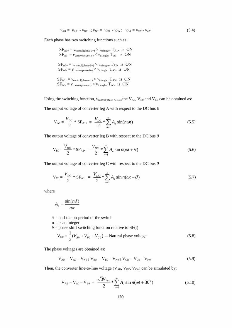
120
vAB = vAN - vBN ; vBC = vBN - vCN ; vCA = vCN - vAN (5.4)
Each phase has two switching functions such as:
SFA1+ = vcontrol(phase-a+) > vtriangle, TA1+ is ON
SFA1- = vcontrol(phase-a-) < vtriangle, TA1- is ON
SFA2+ = vcontrol(phase-b+) > vtriangle, TA2+ is ON
SFA2- = vcontrol(phase-b-) < vtriangle, TA2- is ON
SFA3+ = vcontrol(phase-c+) > vtriangle, TA3+ is ON
SFA3- = vcontrol(phase-c-) < vtriangle, TA3- is ON
Using the switching function, vcontrol(phase-A,B,C) the VA0, VB0 and VC0 can be obtained as:
The output voltage of converter leg A with respect to the DC bus 0
VA0 = 2
DCV* SFA1+ =
1
)sin(*2 n
n
DC tnAV
(5.5)
The output voltage of converter leg B with respect to the DC bus 0
VB0 = 2
DCV* SFA2+ = )(sin*
2 1
tnAV
n
n
DC (5.6)
The output voltage of converter leg C with respect to the DC bus 0
VC0 = 2
DCV* SFA3+ = )(sin*
2 1
tnAV
n
n
DC (5.7)
where
n
nAn
)sin(
= half the on-period of the switch
n = is an integer
θ = phase shift switching function relative to SF(t)
VN0 = )(3
1000 CBA VVV -- Natural phase voltage (5.8)
The phase voltages are obtained as:
VAN = VA0 – VN0 ; VBN = VB0 – VN0 ; VCN = VC0 – VN0 (5.9)
Then, the converter line-to-line voltage (VAB, VBC, VCA) can be simulated by:
VAB = VA0 – VB0 =
1
0 )30(sin*2
3
n
n
DC tnAV
(5.10)

121
VBC = VB0 – VC0 =
1
0 )90(sin*2
3
n
n
DC tnAV
(5.12)
VCA = VC0 – VA0 =
1
0 )150(sin*2
3
n
n
DC tnAV
(5.13)
For the SPWM technique in Fig. 5.2, a triangular carrier waveform (Vtri) is compared
with the reference sinusoidal waveform (Vmod) at the fundamental frequency of the
output voltage. Then, the switching pulses are (SFA1+; SFA1-), (SFA2+; SFA2-), and (SFA3+;
SFA3-), for phase A, phase B and phase C respectively. With these modulated
waveforms, the two-level switching functions ( tSa ; tSb ; tSc ) for each leg of the
AC/DC converter shown in Fig. 5.3 can be expressed as:
112
1AAa SFSFtS (5.14)
222
1AAb SFSFtS (5.15)
332
1AAc SFSFtS (5.16)

122
0 100 200 300 400 500 600-1
0
1
0 100 200 300 400 500 600-1
0
1
0 100 200 300 400 500 600-1
0
1
One cycle
0 20 40 60 80 100 1200
1
2
0 20 40 60 80 100 1200
1
2
0 20 40 60 80 100 1200
1
2
Harmonics
Figure 5.3. Two-level Phase Switching Function of a VSC one Unipolar PWM
Converter (a)Output voltage of phase a and phase b; (b) The amplitude of all harmonic
spectrum for the output voltage of phase a and phase b; (c) Output voltage of phase b
and phase c; (d) The amplitude of all harmonic spectrum for the output voltage of phase
b and phase c; (e) Output voltage of phase c and phase a; (f) The amplitude of all
harmonic spectrum for the output voltage of phase c and phase a
A PWM switching waveform, using a signal carrier based control method with an
average valve switching frequency of 1250 Hz, also with no voltage ripple in the DC
capacitor (ie an infinite capacitance) is shown in Figure 5.3 (a,c,e), each waveform takes
three values (VDC, 0, - VDC) and there is a 120o phase-shift between them. In order to
improve the quality of the output waveform, the converter is typically controlled using
PWM-unipolar, resulting in the output waveform with significant high-order harmonics.
When the waveforms are zero for each half of the period, they will have a 60o interval in
between them and a total of 120o per period. The ratio of the amplitude of the sinusoidal
waveforms with respect to the amplitude of the triangular wave sets the amplitude
modulation ratio. For a system in which the converter sources have impedance loads
and antiparallel diode, in such case the converter operates in all the four quadrants. Each
leg can handle current in both directions at any time, since either the turned on switch or
the antiparallel diode of the other switch can be the conducting element depending upon
the polarity of the output line current. The DC bus capacitor provides the required
energy such that power flow can be controlled and DC harmonics carefully eliminated.
The harmonic spectrums in a 1kHz system associated with the switching function of
(a) (b)
(c) (d)
(e) (f)
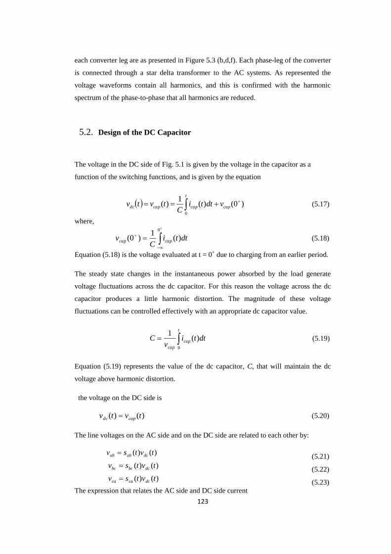
123
each converter leg are as presented in Figure 5.3 (b,d,f). Each phase-leg of the converter
is connected through a star delta transformer to the AC systems. As represented the
voltage waveforms contain all harmonics, and this is confirmed with the harmonic
spectrum of the phase-to-phase that all harmonics are reduced.
5.2. Design of the DC Capacitor
The voltage in the DC side of Fig. 5.1 is given by the voltage in the capacitor as a
function of the switching functions, and is given by the equation
t
capcapcapdc vdttiC
tvtv0
)0()(1
)( (5.17)
where,
dttiC
v capcap )(1
)0(
0
(5.18)
Equation (5.18) is the voltage evaluated at t = 0+ due to charging from an earlier period.
The steady state changes in the instantaneous power absorbed by the load generate
voltage fluctuations across the dc capacitor. For this reason the voltage across the dc
capacitor produces a little harmonic distortion. The magnitude of these voltage
fluctuations can be controlled effectively with an appropriate dc capacitor value.
t
cap
cap
dttiv
C0
)(1
(5.19)
Equation (5.19) represents the value of the dc capacitor, C, that will maintain the dc
voltage above harmonic distortion.
the voltage on the DC side is
)()( tvtv capdc (5.20)
The line voltages on the AC side and on the DC side are related to each other by:
)()( tvtsv dcabab (5.21)
)()( tvtsv dcbcbc (5.22)
)()( tvtsv dccaca (5.23)
The expression that relates the AC side and DC side current

124
iDC(t) = Sab(t) iab(t) + Sbc(t) ibc (t) + Sca(t) ica(t) (5.24)
In the harmonic domain Equ (5.14) may be represented as
Vcap = C
1D
-1(jh 0 )Idc + Edc (5.25)
where
Vcap is assembled with the harmonic content of vcap(t)
Idc is assembled with the harmonic content of idc(t)
Edc contains only a DC term, i.e.
Edc = [0 0 vcap(0+) 0 0]
T
The equivalent impedance of the capacitor on the DC side is given as
Zcap = C
1D
-1(jh 0 ) (5.26)
Therefore, (5.25) can be represented as
Vcap = Zcap Idc + Edc (5.27)
Also, (5.20) and (5.21) the voltage on the DC side and its relationship to the AC phase
voltages may be represented in the harmonic domain as
Vdc = Vcap (5.28)
Va = Sab Vdc
Vb = Sbc Vdc (5.29)
Vc = Sca Vdc
Similarly, the relationship between the line currents and the DC is represented in
harmonics domain as
Idc = Sab Ia + Sbc Ib + Sca Ic (5.30)
5.3. Modular Multi-Level VSC with PWM-Unipolar
Multilevel converter technology has experienced increasing attention in the last decade,
and several topologies have been reported [35][36]. From the traditional topology of H-
bridge converter, a new topology named modular multi-level converter (MMC) is
developed, which has the capability of generating multi-level output voltage waveforms.
By using two or more sub-modules cascaded connection with additional DC capacitors,
a flexible three-phase cascaded H-bridge VSC is formed. This H-bridge converter is
expanded to develop three legs per phase connected to three-phase electromagnetic
interface without any filter equipment. As shown each arm is composed of three or

125
more sub-modules with additional central capacitive energy storage at the DC side. The
proposed model has the capability of generating multi-levels (two-level, four-level and
six-level, etc) voltage waveforms. Each sub-module of the converter consists of three
legs similar to the conventional three-phase VSC, which is minimum power unit of
MMC. In which DA1+, DA1-, DA2+, DA2-, DA3+, and DA3- are the diodes of IGBTs. This
IGBT valve consists of IGBT module with its freewheeling diode (FWD) and
auxiliary’s snubbed circuit. The cascaded connected SM is aimed at increasing the
output voltage waveforms and power quality operational characteristics, which can be
termed as the expansion of three phase IGBT module [37][38]. Though MMC valves
are not only used to increasing voltage levels but also has good driver and controller
attributes. This sophisticated topology opens doors for more cancellation of harmonics
with proper phase-shifting comparable to conventional VSCs. With this configuration,
the harmonic content of the output voltage is reduced and the harmonic elimination at
the magnetic interface level can be achieved without increasing the switching
frequencies in the PWM control system.
Phase shifting is an important parameter for the control of modular converters in order
to achieve high quality output voltage waveforms. It magnetically cancels lower order
harmonics such 5th and 7
th, even if they are not equal in magnitude. Each cascaded
three-phase MMC converter uses PWM uni-polar voltage switching. The number of
levels per phase half cycle of the switching function sni(t), where SMni is the cell sub-
module, is given by the frequency modulation ratio mf,
s
rf
f
fm
(5.31)
where,
f r = triangular frequency and f s = sinusoidal
the harmonics generated by the voltage converter i are given by
h = 2jmf k where j,k = 1,2,3,... (5.32)
h are the harmonics of sni(t)
The shifted angles for the cell sub-module (SMni) carrier signal are given by
iri ni /)1(2 (5.33)

126
By using cell sub-module MMC-PWM converters in parallel, the harmonics generated
by the VSC-MMC are given as
h = 2jmf k where j,k = 1,2,3,... (5.34)
the magnitudes of the harmonics are given as
ni
SMSMSMSMS anaaa
MMC
321 (5.35)
where the magnitude of the fundamental frequency component has a value of
modulation index (m).
It should be noted that an increase in the voltage ratings (which is imposed by the
application) has a direct impact in the Cascaded H-Bridge (CHB) MMC power quality,
due to the increase in the number of the output voltage levels and the increase of the
number of input-current pulses, both leading to output- and input-quality improvements,
respectively
The topology of MMCs with three-phase cascaded H-bridge (CHB) per phase is as
depicted in Fig. 5.4. This topology is suitable for MV high-power drives and high
voltage applications (HV), due to its modular structure and power-quality operational
characteristics and could gain popularity in the future. One advantage of this topology is
that, there is no need for a voltage balancing stabilizer. Owing to the fact that, the input
transformer has the provision for independent and isolated DC sources at the secondary
windings side. The capacitor voltage does not required huge initialization. The
configuration of CHB MMC permits series connection to achieve high voltage levels for
high power application, used in oil and gas exploration and production fields. The
topology offers very high power voltage waveforms and lower switching losses,
because the high power sub-modules only commutate at fundamental switching
frequency. The CHB can be more adapted to operate under internal fault conditions. In a
case where one of the sub-modules is reported to be faulty, a simply bypassing faulty
cell can be employed with ease to enhance operation. The model uses phase shifted
transformer with PWM control technique to cancel more harmonics, even at a low
frequency. Each PWM converter (sub-module) is capable of generating more than two-
level voltage waveform across the three mid-point legs.

127
Figure 5.4: Modular Multi-Level Three-Phase VSC
5.4. Multilevel Output-Voltage Generation
Consider the topology of the power sub-modules presented in Fig. 5.4. The switching
state of one sub-module SMa is determined by the logical value of three signals (TA1+,
+
-
C C C
SMa1
SMa2
SMa3
SMan
SMb1
SMb
2
SMb3
SMb
n
SMc1
SMc2
SMc3
SMcn
Q, P
iiV
PCC
Impedance
Magnetic interface
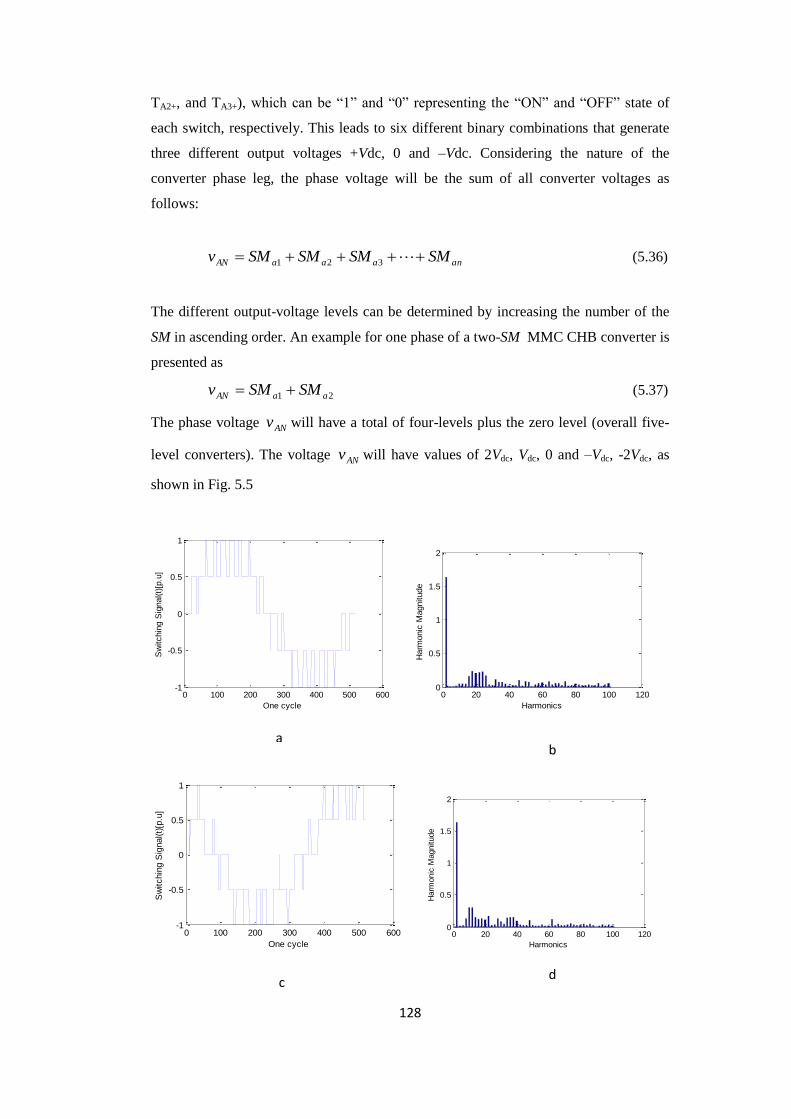
128
TA2+, and TA3+), which can be “1” and “0” representing the “ON” and “OFF” state of
each switch, respectively. This leads to six different binary combinations that generate
three different output voltages +Vdc, 0 and –Vdc. Considering the nature of the
converter phase leg, the phase voltage will be the sum of all converter voltages as
follows:
anaaaAN SMSMSMSMv 321 (5.36)
The different output-voltage levels can be determined by increasing the number of the
SM in ascending order. An example for one phase of a two-SM MMC CHB converter is
presented as
21 aaAN SMSMv (5.37)
The phase voltage ANv will have a total of four-levels plus the zero level (overall five-
level converters). The voltage ANv will have values of 2Vdc, Vdc, 0 and –Vdc, -2Vdc, as
shown in Fig. 5.5
0 100 200 300 400 500 600-1
-0.5
0
0.5
1
One cycle
Sw
itchin
g S
ignal(t)
[p.u
]
0 20 40 60 80 100 120
0
0.5
1
1.5
2
Harmonics
Harm
onic
Magnitude
0 100 200 300 400 500 600-1
-0.5
0
0.5
1
One cycle
Sw
itchin
g S
ignal(t)
[p.u
]
0 20 40 60 80 100 120
0
0.5
1
1.5
2
Harmonics
Harm
onic
Magnitude
a b
c d
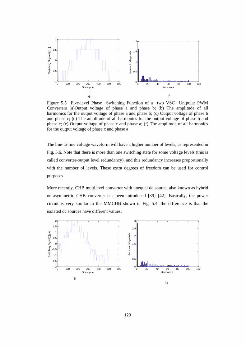
129
0 100 200 300 400 500 600-1
-0.5
0
0.5
1
One cycle
Sw
itchin
g S
ignal(t)
[p.u
]
0 20 40 60 80 100 120
0
0.5
1
1.5
2
Harmonics
Harm
onic
Magnitude
Figure 5.5 Five-level Phase Switching Function of a two VSC Unipolar PWM
Converters (a)Output voltage of phase a and phase b; (b) The amplitude of all
harmonics for the output voltage of phase a and phase b; (c) Output voltage of phase b
and phase c; (d) The amplitude of all harmonics for the output voltage of phase b and
phase c; (e) Output voltage of phase c and phase a; (f) The amplitude of all harmonics
for the output voltage of phase c and phase a
The line-to-line voltage waveform will have a higher number of levels, as represented in
Fig. 5.6. Note that there is more than one switching state for some voltage levels (this is
called converter-output level redundancy), and this redundancy increases proportionally
with the number of levels. These extra degrees of freedom can be used for control
purposes.
More recently, CHB multilevel converter with unequal dc source, also known as hybrid
or asymmetric CHB converter has been introduced [39]–[42]. Basically, the power
circuit is very similar to the MMCHB shown in Fig. 5.4, the difference is that the
isolated dc sources have different values.
0 100 200 300 400 500 600-2
-1.5
-1
-0.5
0
0.5
1
1.5
2
One cycle
Sw
itchin
g S
ignal(t)
[p.u
]
0 20 40 60 80 100 1200
0.5
1
1.5
2
2.5
3
Harmonics
Harm
onic
Magnitude
e f
a b
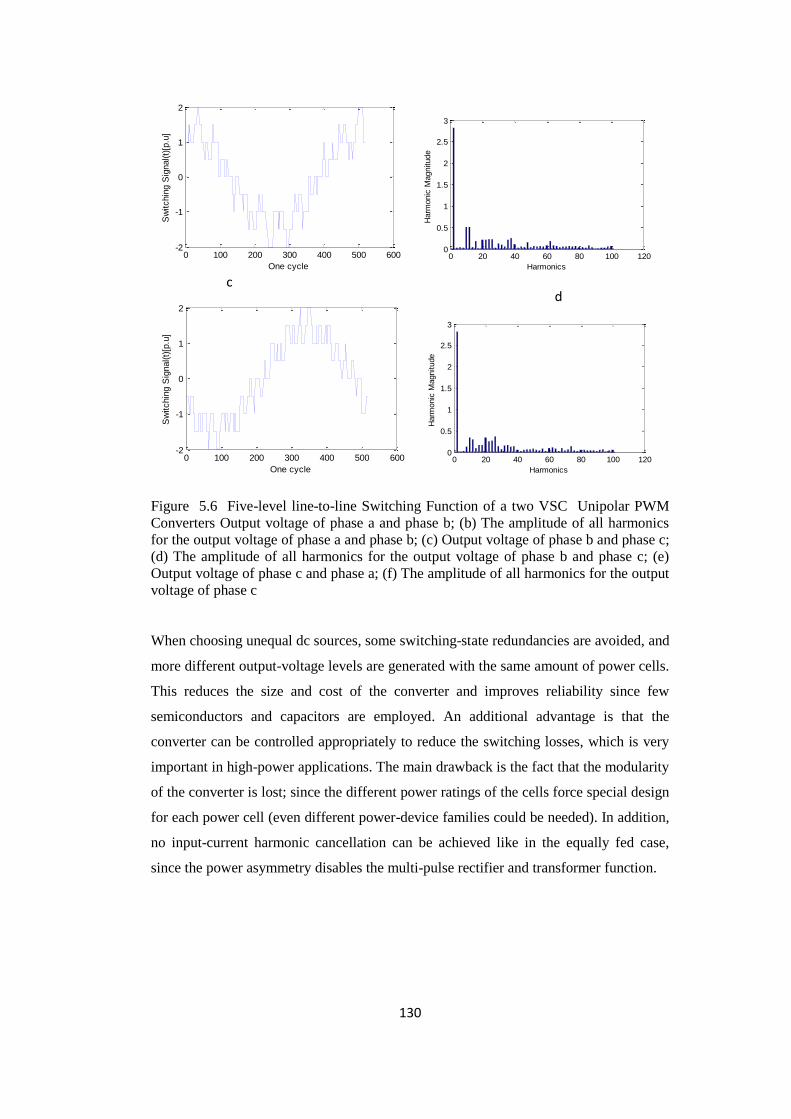
130
0 100 200 300 400 500 600-2
-1
0
1
2
One cycle
Sw
itchin
g S
ignal(t)
[p.u
]
0 20 40 60 80 100 1200
0.5
1
1.5
2
2.5
3
Harmonics
Harm
onic
Magnitude
0 100 200 300 400 500 600-2
-1
0
1
2
One cycle
Sw
itchin
g S
ignal(t)
[p.u
]
0 20 40 60 80 100 1200
0.5
1
1.5
2
2.5
3
Harmonics
Harm
onic
Magnitude
Figure 5.6 Five-level line-to-line Switching Function of a two VSC Unipolar PWM
Converters Output voltage of phase a and phase b; (b) The amplitude of all harmonics
for the output voltage of phase a and phase b; (c) Output voltage of phase b and phase c;
(d) The amplitude of all harmonics for the output voltage of phase b and phase c; (e)
Output voltage of phase c and phase a; (f) The amplitude of all harmonics for the output
voltage of phase c
When choosing unequal dc sources, some switching-state redundancies are avoided, and
more different output-voltage levels are generated with the same amount of power cells.
This reduces the size and cost of the converter and improves reliability since few
semiconductors and capacitors are employed. An additional advantage is that the
converter can be controlled appropriately to reduce the switching losses, which is very
important in high-power applications. The main drawback is the fact that the modularity
of the converter is lost; since the different power ratings of the cells force special design
for each power cell (even different power-device families could be needed). In addition,
no input-current harmonic cancellation can be achieved like in the equally fed case,
since the power asymmetry disables the multi-pulse rectifier and transformer function.
c d

131
5.5. Modulation Method and Simulations Results
Phase-shifted PWM (PS-PWM) is the natural PWM method for CHB [43], mainly due
to the modularity of this topology. Each cell is modulated independently using unipolar
PWM with the same reference signal. A phase shift is introduced across all the carrier
signals of each SM in order to produce the stepped multilevel waveform. The lowest
output-voltage distortion is achieved with 180o/n phase shifts between the carriers, for a
k-SM converter. This operating principle is shown for a three SM seven level in Fig.
5.7. Note how the converter-output voltage has k times the fundamental component of
each SM. In addition, the frequency of the converter-output-voltage switching pattern is
k times the SM switching frequency, since the phase shift introduces a multiplicative
effect. This is very useful, since the device switching frequency (hence, the switching
losses) is k times lower than the apparent switching frequency perceived by the load.
This means that, for the same output switching frequency, phase-shifted produces k
times less switching losses as compared to level-shifted. However, level-shifted leads to
less distorted line voltages since all the carriers are in phase [44].
Since all the SMs are controlled with the same reference and the same carrier frequency,
the power is evenly distributed among the SMs, achieving input-current harmonic
reduction owing to the multi-pulse transformer–rectifier system [43].
For low-switching-frequency applications, the staircase modulation is used. The basic
idea of this technique is to connect each SM of the converter at specific angles to
generate the multilevel output waveform, producing only a minimum of necessary
commutations [44].
0 100 200 300 400 500 600-1
-0.5
0
0.5
1
One cycle
Sw
itchin
g S
ignal(t)
[p.u
]
0 20 40 60 80 100 1200
0.5
1
1.5
2
Harmonics
Harm
onic
Magnitude
a b

132
0 100 200 300 400 500 600-1
-0.5
0
0.5
1
One cycle
Sw
itchin
g S
ignal(t)
[p.u
]
0 20 40 60 80 100 120
0
0.5
1
1.5
2
Harmonics
Harm
onic
Magnitude
0 100 200 300 400 500 600-1
-0.5
0
0.5
1
One cycle
Sw
itchin
g S
ignal(t)
[p.u
]
0 20 40 60 80 100 120
0
0.5
1
1.5
2
Harmonics
Harm
onic
Magnitude
Figure 5.7 Seven-level Phase Switching Function of a three VSC Unipolar PWM
Converters Output voltage of phase a and phase b; (b) The amplitude of all harmonics
for the output voltage of phase a and phase b; (c) Output voltage of phase b and phase c;
(d) The amplitude of all harmonics for the output voltage of phase b and phase c; (e)
Output voltage of phase c and phase a; (f) The amplitude of all harmonics for the output
voltage of phase c and phase a
0 100 200 300 400 500 600-2
-1.5
-1
-0.5
0
0.5
1
1.5
2
One cycle
Sw
itchin
g S
ignal(t)
[p.u
]
0 20 40 60 80 100 120
0
0.5
1
1.5
2
2.5
3
Harmonics
Harm
onic
Magnitude
c d
e f
a b
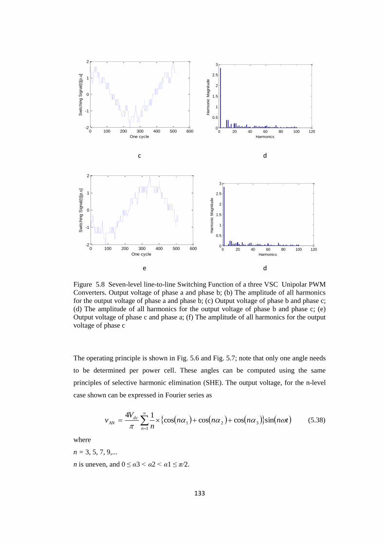
133
0 100 200 300 400 500 600-2
-1
0
1
2
One cycle
Sw
itchin
g S
ignal(t)
[p.u
]
0 20 40 60 80 100 120
0
0.5
1
1.5
2
2.5
3
Harmonics
Harm
onic
Magnitude
0 100 200 300 400 500 600-2
-1
0
1
2
One cycle
Sw
itchin
g S
ignal(t)
[p.u
]
0 20 40 60 80 100 120
0
0.5
1
1.5
2
2.5
3
Harmonics
Harm
onic
Magnitude
Figure 5.8 Seven-level line-to-line Switching Function of a three VSC Unipolar PWM
Converters. Output voltage of phase a and phase b; (b) The amplitude of all harmonics
for the output voltage of phase a and phase b; (c) Output voltage of phase b and phase c;
(d) The amplitude of all harmonics for the output voltage of phase b and phase c; (e)
Output voltage of phase c and phase a; (f) The amplitude of all harmonics for the output
voltage of phase c
The operating principle is shown in Fig. 5.6 and Fig. 5.7; note that only one angle needs
to be determined per power cell. These angles can be computed using the same
principles of selective harmonic elimination (SHE). The output voltage, for the n-level
case shown can be expressed in Fourier series as
tnnnnn
Vv
n
dc
AN
sincoscoscos14
321
1
(5.38)
where
n = 3, 5, 7, 9,...
n is uneven, and 0 ≤ α3 < α2 < α1 ≤ π/2.
c d
e d

134
The three coefficients of the Fourier series (5.38) can be forced to a desired value;
naturally, the first coefficient corresponds to the fundamental component and is set to
the desired modulation index while, usually, the fifth and seventh coefficient are set to
zero to eliminate 5th and 7
th harmonics as follows
321 coscoscos4
M
321 5cos5cos5cos0
321 7cos7cos7cos0 (5.39)
where
dc
AN
kV
vM is the modulation index, defined by the desired peak amplitude for the
fundamental component of the output voltage ANv and
k = 1,2,3,... is the number of SM cells
The main advantage of MMCHB, is that the converter switches very few times per
cycle, reducing the switching losses to a minimum. In addition, there is a reduction in
all harmonics as the number of SM cells increases, therefore facilitating the output-filter
design.
The hybrid modulation is particularly conceived for the MMCHB with unequal dc
sources. The basic idea is to take advantage of the different power ratings among the
cells to reduce switching losses and improve the converter efficiency. For example,
from Fig. 5.9 and Fig. 5.10, it is shown that the high-power cell will turn on and off
only one time during a half reference cycle. The un-modulated part left by the square
shape of the high-power cell output is then generated by the next power cell and so on,
until the final un-modulated parts of the reference are modulated at high switching
frequency (with unipolar sinusoidal PWM) by the smallest power cell. This completes
the generation of a multilevel stepped waveform with a high-frequency component
(similar to multicarrier based PWM) but with the difference that fewer switching losses
are produced to achieve it.

135
0 100 200 300 400 500 600-1
-0.5
0
0.5
1
One cycle
Sw
itchin
g S
ignal(t)
[p.u
]
0 20 40 60 80 100 1200
0.5
1
1.5
2
Harmonics
Harm
onic
Magnitude
0 100 200 300 400 500 600-1
-0.5
0
0.5
1
One cycle
Sw
itchin
g S
ignal(t)
[p.u
]
0 20 40 60 80 100 1200
0.5
1
1.5
2
Harmonics
Harm
onic
Magnitude
0 100 200 300 400 500 600-1
-0.5
0
0.5
1
One cycle
Sw
itchin
g S
ignal(t)
[p.u
]
0 20 40 60 80 100 1200
0.5
1
1.5
2
Harmonics
Harm
onic
Magnitude
Figure 5.9 Nine-level Phase Switching Function of a fourVSC Unipolar PWM
Converters. Output voltage of phase a and phase b; (b) The amplitude of all harmonics
for the output voltage of phase a and phase b; (c) Output voltage of phase b and phase c;
(d) The amplitude of all harmonics for the output voltage of phase b and phase c; (e)
Output voltage of phase c and phase a; (f) The amplitude of all harmonics for the output
voltage of phase c and phase a
a b
c d
e f

136
0 100 200 300 400 500 600-2
-1.5
-1
-0.5
0
0.5
1
1.5
2
One cycle
Sw
itchin
g S
ignal(t)
[p.u
]
0 20 40 60 80 100 120
0
0.5
1
1.5
2
2.5
3
Harmonics
Harm
onic
Magnitude
0 100 200 300 400 500 600-2
-1
0
1
2
One cycle
Sw
itchin
g S
ignal(t)
[p.u
]
Harmonics
Harm
onic
Magnitude
Harmonics
Harm
onic
Magnitude
Harmonics
Harm
onic
Magnitude
0 20 40 60 80 100 120
0
0.5
1
1.5
2
2.5
3
Harmonics
Harm
onic
Magnitude
0 100 200 300 400 500 600-2
-1
0
1
2
One cycle
Sw
itchin
g S
ignal(t)
[p.u
]
0 20 40 60 80 100 120
0
0.5
1
1.5
2
2.5
3
Harmonics
Harm
onic
Magnitude
Figure 5.10 Nine-level line-to-line Switching Function of a four VSC Unipolar PWM
Converters. Output voltage of phase a and phase b; (b) The amplitude of all harmonics
for the output voltage of phase a and phase b; (c) Output voltage of phase b and phase c;
(d) The amplitude of all harmonics for the output voltage of phase b and phase c; (e)
Output voltage of phase c and phase a; (f) The amplitude of all harmonics for the output
voltage of phase c
a b
c d
e f

137
It should be noted that the high-voltage cell commutates when the reference reaches a
specific voltage level hn. This level needs to be selected in such a way that the un-
modulated part can be generated by the lower power cells to avoid over-modulation. If
we consider that the maximum amplitude that can be generated by the converter as
shown in Fig. 5.9 and Fig. 5.10 are V1 + V2 + V3+ V4 0 -V1 -V2 -V3-V4 the only
possibility to avoid over-modulation is that the un-modulated part does not exceed the
total voltage left for the low-power cells of the converter, i.e., h4 = V1 + V2 + V3+ V4.
Hence, must be h3 = V1 + V2 + V3 for the third power cell with traditional unipolar
PWM.
The distortion of the voltage waveforms, harmonic losses in the power converter and the
load are due to the operation in the switching mode. These highlight the comparison of
power qualities of the different output voltage levels with the PWM-unipolar control
method. The simulations of individual frequency components to a voltage waveform are
expressed in a harmonic voltage spectrum, which give more detailed harmonic
description than the output voltage waveform as shown in Fig. 5.11 and Fig. 5.12. The
simulations data are as follows: h = 100; % h is the number of harmonics to be
calculated. E = 1.2; % E is the DC capacitor voltage. C = 10^-3; % C is the capacitor in
the DC side, farads. f = 1000; % f is the frequency in Hz. w = 2*pi*f; % angular
frequency. hr = 5; % is the harmonic frequency of the carrier signal. mf = 5 ;% freq
modulation index = triangular frequency (250)/sinusoidal frequency(50) . ma = 0.8; %
ma is the voltage modulation index = sinusoidal amplitude/triangular amplitude. nc = 4;
% Number of converter.
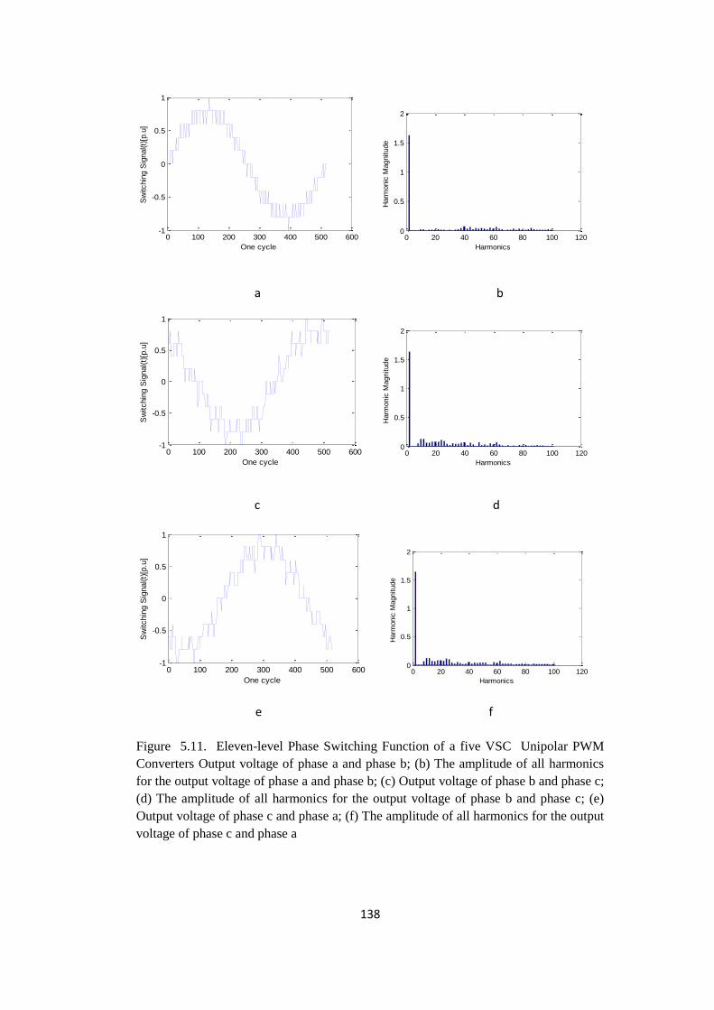
138
0 100 200 300 400 500 600-1
-0.5
0
0.5
1
One cycle
Sw
itchin
g S
ignal(t)
[p.u
]
0 20 40 60 80 100 120
0
0.5
1
1.5
2
Harmonics
Harm
onic
Magnitude
0 100 200 300 400 500 600-1
-0.5
0
0.5
1
One cycle
Sw
itchin
g S
ignal(t)
[p.u
]
0 20 40 60 80 100 1200
0.5
1
1.5
2
Harmonics
Harm
onic
Magnitude
0 100 200 300 400 500 600-1
-0.5
0
0.5
1
One cycle
Sw
itchin
g S
ignal(t)
[p.u
]
0 20 40 60 80 100 120
0
0.5
1
1.5
2
Harmonics
Harm
onic
Magnitude
Figure 5.11. Eleven-level Phase Switching Function of a five VSC Unipolar PWM
Converters Output voltage of phase a and phase b; (b) The amplitude of all harmonics
for the output voltage of phase a and phase b; (c) Output voltage of phase b and phase c;
(d) The amplitude of all harmonics for the output voltage of phase b and phase c; (e)
Output voltage of phase c and phase a; (f) The amplitude of all harmonics for the output
voltage of phase c and phase a
a b
c d
e f

139
0 100 200 300 400 500 600-2
-1.5
-1
-0.5
0
0.5
1
1.5
2
One cycle
Sw
itchin
g S
ignal(t)
[p.u
]
0 20 40 60 80 100 120
0
0.5
1
1.5
2
2.5
3
Harmonics
Harm
onic
Magnitude
0 100 200 300 400 500 600-2
-1
0
1
2
One cycle
Sw
itchin
g S
ignal(t)
[p.u
]
0 20 40 60 80 100 120
0
0.5
1
1.5
2
2.5
3
Harmonics
Harm
onic
Magnitude
0 100 200 300 400 500 600-2
-1
0
1
2
One cycle
Sw
itchin
g S
ignal(t)
[p.u
]
0 20 40 60 80 100 120
0
0.5
1
1.5
2
2.5
3
Harmonics
Harm
onic
Magnitude
Figure 5.12. Eleven-level line-to-line Switching Function of a five VSC Unipolar
PWM Converters Output voltage of phase a and phase b; (b) The amplitude of all
harmonics for the output voltage of phase a and phase b; (c) Output voltage of phase b
and phase c; (d) The amplitude of all harmonics for the output voltage of phase b and
phase c; (e) Output voltage of phase c and phase a; (f) The amplitude of all harmonics
for the output voltage of phase c
a b
c d
e f

140
The number of output phase voltage levels in a cascade multilevel converter is then 2s
+1, where s is the number of dc sources. Simulated phase voltage waveform for an 11-
level cascaded multilevel converter with five separate dc sources SDSCs (s = 5) and five
full bridges is shown in Fig. 5.18. The output phase voltage is given by
van = V1 + V2 + V3+ V4 + V5 (5.40)
With enough levels and an appropriate switching algorithm, the multilevel converter
results in an output voltage that is almost sinusoidal as shown in Fig. 5.12.
As observed the phase output voltage has better output power quality as shown in Fig.
5.11 comparable to the line-to-line output voltage waveform as shown in Fig. 5.12. By
increasing number of the SM of the network reduces all harmonics to a minimum and
also improves voltage profiles and reduces power system losses. Lower harmonic
contents require a higher current flow for a given load. Increase in the line current
results in a high voltage distortion at the converter output. With a reduction in the
harmonic content, the voltage distortion is reduced.
When the converters are in operation they produce electromagnetic interference with
harmonic content, thus reducing power quality. On this scenario, PWM-unipolar can be
used to eliminate harmonic contents and permit additional submodules to be added to an
existing facility and also, provide high power drives at electromagnetic interface to high
voltage network. The achievement of power quality using PWM-unipolar control could
become an important issue to transmission and distribution engineers.
The reduction in switching function losses vary from lower number of submodules to
higher number submodules of the total PWM-unipolar converters. The financial benefit
from switching loss reduction is enough to justify the MMC PWM-unipolar technique.
The switching functions losses are proportional to the voltage and current output
waveforms reduced harmonic distortion.
From the harmonic spectrum the harmonics occur as side bands of 2mf and its integral
multiple. As identified the frequencies of the harmonics are doubled, owing to the
utilization of a unipolar switching scheme. This results in a reduction in the lower order
141
harmonics. This order of harmonics is as given by (5.29). It should be noted here that
the fundamental component has a peak value equal to ma times the source voltage.
In this type of converter, the only states that have no redundant configurations are the
two states that generate the maximum positive and negative voltages, + VDC/2 and –
VDC/2. For generating the other levels, IGBT-PWM is the possible switching
configuration that keeps the capacitor voltages balanced. The switching sequence is
controlled such that at each instant only SMans (i.e. half of the 2SMans of a phase leg)
are in the on-state. The upper arm SMs from SMa1 to SMan are in the on-state, in the
lower arm only SMa2 to SMan will be in on-state. It is clear that there are several
possible switching configurations. Equal voltage sharing among the capacitor of each
arm was achieved by unipolar algorithm of inserted SMans during each sampling period
of the control system.
5.6. Conclusions
A new topology, modular multi-level converter using PWM-unipolar switching
technique for harmonic reduction is developed. The output voltage waveforms of the
IGBTs are controlled using a PWM-unipolar technique to achieve the minimum
harmonic reduction.
The MMC is suitable for reducing wave power harmonic voltage to a minimum level,
and has the capability for stabilization of the voltage and current in the high voltage oil
and gas network exploration and production
The line-to-line voltage is able to synthesize more levels compared to the phase voltage,
thus resembling a more desirable sinusoidal waveform. Besides that, the phase voltage
yields better spectral performance, hence reducing the need of an output filter.
The number of output waveform levels is higher than the level of the converters, hence
leads to output power quality improvement.
The switching functions, based on Complex Fourier Series, are used effectively to
demonstrate the operation of the MMC. The optimum harmonic reductions of this
developed model are proportional to the increase in the number of VSC sub-modules.

142
5.7. References
[1] J.S.Lai, and F.Z.Peng,“Multilevel Converters – A new breed of power converters”,
IEEE Trans. Ind. Applicat., vol. 32, pp 509-517, May./June. 1996
[2] J. Rodriguez, J.Sheng. Lai, F. Z. Peng, “Multilevel Inverters: A survey of
topologies, controls, and applications”, IEEE Trans. Ind. Electr., vol. 49, pp 724-
738, Aug. 2002
[3] H. Akagi, “Classification, Terminology, and Application of the Modular
MultilevelCascade Converter (MMCC)”. IEEE International Power Electronics
Conference, 2010.
[4] F.Z.Peng, J. W. McKeever, D. J. Adams,“Cascade Multilevel Inverters for Utility
Applications.” IEEE Industrial Electronics, Control and Instrumentation
Conference (IECON), 1997.
[5] F.Z. Peng. J. S. Lai, “Dynamic Performance and Control of a Static Var Generator
using Multilevel Inverters.” IEEE Transactions on Industrial Applications, vol.
33, May/June 1997.
[6] L.M. Tolbert and F. Z. Peng, “Multilevel Converters as a Utility Interface for
Renewable Energy Systems.” IEEE 2000.
[7] S. Sirisukprasert, A.Q. Huang and J.S. Lai, “ Modelling, Analysis and Control of
Cascaded-Multilevel Converter-Based STATCOM”. IEEE 2003.
[8] J. Rodriguez, J.-S. Lai, and F.Z. Peng, “Multilevel Inverters: A Survey of
Topologies, Controls, and Applications.” IEEE Trans. Ind. Electronics, vol. 49,
Aug. 2002.
[9] Q. Tu, Z. Xu, H. Huang and J. Zhang, “Parameter Design Principle of the Arm
Induction in Modular Multilevel Converter based HVDC”. International
Conference on Power System Technolgy, 2010 IEEE.
[10] A.L.P. de Oliveira, C.E. Tiburcio, M.N. Lemes and D. Retzmann, “Prospects of
Voltage-Sourced Converters (VSC) Application in Power Transmission
Systems”. IEEE ANDESCON 2010.
[11] A. Lesnicar and R. Marquardt, “An Innovative Modular Multilevel Converter
Topology Suitable for a Wide Power Range”. PowerTech Conference. 2003 IEEE
.
[12] K.Li and C.Zhao, “New Technologies of Modular Multilevel Converter for VSC-
HVDC Application”. 2010 IEEE.
[13] A. Rasic, U. Krebs and H. Leu, “Optimization of the Modular Multilevel
Converters Performance using the Second Harmonic of the Module Current”.
URL: http://www.siemens.com
[14] X. Luo, G.F. Tang, K.P. Zha, Z.Y. He, and Y.N. Wu, “Study on the Design and
Equivalence Test Methods of VSC-HVDC Valves”. International Conference on
Power System Technolgy, 2010 IEEE.

143
[15] J. Rodrigues, S. Bernet, B. Wu, J. O. Pontt and S. Kouro, “ Multilevel Voltage-
Source-Converter Topologies for Industrial Medium-Voltage Drives”. IEEE
Transactions on Industrial Electronics, VOL. 54. 2007.
[16] M. Saeedifard and R. Iravani, “Dynamic Performance of a Modular Multilevel
Back-to-Back HVDC System”. IEEE Transactions on Power Delivery, VOL. 25.
2010
[17] J.S. Lai, F. Z. Peng, “Multilevel Converter-A New Breed of Power Converter”.
IEEE Transactions on Industrial Applications. Vol. 32. 1996.
[18] C. Casablanca and J. Sun, “Interleaving and Harmonic Cancellation Effects in
Modular Three-Phase Voltage-Sourced Converters”. IEEE COMPEL Workshop,
July 16-19, 2006.
[19] U.N.Gnanarathna, S.K.Chaudhary, A.M. Gole, and R. Teodrescu.“ Modular
Multi-level Converter Based HVDC System for Grid Connection of Offshore
Wind Power Plant”.
[20] G.Carrara, S. Gardella and M. Marchesoni,“A New Multilevel PWM Method: A
Theoretical Analysis”. IEEE Transactions on Power Electronics, VOL. 3. July
1992.
[21] M. Calais, V.G. Agelidis and M. Meinhardt, “Multilevel Conveters for Single-
Phase Grid Connected Photovoltaic Systems: An Overview”. Solar Energy vol.
66, 1999.
[22] J.Kim, S. Sul, “A Carrier-Based PWM Method for Three-Phase Four-Leg Voltage
Source Converter”. IEEE Transactions on Power Electronics, VOL. 19. January
2004.
[23] O. A. Sadaba, P. S. Girpide, J. L. Taberna, I. M. Morales, and L. M. Palomo,
“Voltage harmonics generated by 3-level converters using PWM natural
sampling,” in Proc. IEEE Power Electronics Specialist Conf. (PESC), Jun. 2001,
vol. 2, pp. 1561–1565.
[24] J. Hamman and F. S. Van Der Merwe, “Voltage harmonics generated by voltage-
fed inverters using PWM natural sampling,” IEEE Trans. Power Electron., vol. 3,
no. 3, pp. 297–302, Jul. 1988.
[25] R.Ghosh and G.Narayanan, “Control of Three-Phase, Four-Wire PWM Rectifier”,
IEEE Transactions on Power Electronics, vol. 23, No. 1, January 2008
[26] P.H.Zope,P.G.Bhangale, P.Sonare and S.R.Suralkar,“Design and Implementation
of carrier based Sinusoidal PWM Inverter”, International Journal of Advanced
Research in Electrical, Electronics and Instrumentation Engineering, Vol. 1,
Issue 4, October 2012.
[27] B.Ismail,“Development of a Single Phase SPWM Microcontroler -Based Inverter,
First International Power and Energy Conference PEC pp. 437. Putra jaya,
Malaysia: IEEE, November 2006.
[28] R. Teichmann and S. Bernet, “A comparison of three-level converters versus two-
level converters for low-voltage drives, traction, and utility applications,” IEEE
Trans. Ind. Appl., vol. 41, pp. 855–865, May–June 2005.
144
[29] D. M. Mohan, B. Singh and B. K. Panigrahi, “A Two-Level, 48-Pulse Voltage
Source Converter for HVDC Systems”, Fifteenth National Power Systems
Conference (NPSC), IIT Bombay, December 2008.
[30] P.W. Lehn, “Direct Harmonic Analysis of the Voltage Source Converter”, IEEE
Transactions on Power Delivery, Vol. 18, No. 3, July 2003
[31] M.Madrigal and E. Acha, “Modelling of custom power equipment using harmonic
domain techniques,” vol. 1, pp. 264–269, 2000.
[32] P. Lehn, “Exact Modelling of the Voltage Source Converter,” IEEE Trans.Power
Delivery, vol. 17, pp. 217–222, Jan. 2002.
[33] H. Visser and P. van den Bosch, “Modelling of periodically switched networks,”
in IEEE Power Electron. Specialists Conf., 1991, pp. 67–73.
[34] E. Acha and M. Madrigal, “Harmonic Modelling of Voltage Source Converters
for HVDC Station”. AC-DC Power Transmission, Conference Publication. IEE
2001.
[35] J.Rodriguez, S.L a i j and F.Z. Peng, “Multilevel inverters: a survey of topologies,
controls, and applications”, IEEE Trans.Ind. Electron., 49 (2002), No. 4, 724-738
[36] Z. F. Peng, “A Generalized Multilevel Inverter Topology with Self Voltage
Balancing”, Oak Ridge National Laboratory, Oak Ridge, Tennessee 37831-8038
[37] J. Rodríguez, J. Dixon, J. Espinoza, J. Pontt, and P. Lezana, “PWM regenerative
rectifiers: State of the art,” IEEE Trans. Ind. Electron., vol. 52, no. 1, pp. 5–22,
Feb. 2005.
[38] P. Lezana, C. A. Silva, J. Rodriguez, and M. A. Perez, “Zero-steadystate-error
input-current controller for regenerative multilevel converters based on single-
phase cells,” IEEE Trans. Ind. Electron., vol. 54, no. 2, pp. 733–740, Apr. 2007.
[39] O. M. Mueller and J. N. Park, “Quasi-linear IGBT inverter topologies,” in Proc.
APEC, Feb. 1994, pp. 253–259.
[40] S. Mariethoz and A. Rufer, “Design and control of asymmetrical multi-level
inverters,” in Proc. IECON, Sevilla, Spain, Nov. 2002, pp. 840–845.
[41] C. Rech and J. R. Pinheiro, “Line current harmonics reduction in multipulse
connection of asymmetrically loaded rectifiers,” IEEE Trans. Ind. Electron., vol.
52, no. 3, pp. 640–652, Jun. 2005.
[42] C. Rech and J. R. Pinheiro, “Hybrid multilevel converters: Unified analysis and
design considerations,” IEEE Trans. Ind. Electron., vol. 54, no. 2, pp. 1092–
1104, Apr. 2007.
[43] P. Hammond, “A new approach to enhance power quality for medium voltage AC
drives,” IEEE Trans. Ind. Appl., vol. 33, no. 1, pp. 202–208, Jan./Feb. 1997.
[44] D.G. Holmes and T. Lipo,“PulseWidth Modulation for Power Converters:
Principles and Practice”. Piscataway, NJ: IEEE Press, 2003.
[45] B. Wu, “High-Power Converters and AC Drives”. Piscataway, NJ: IEEE Press,
2006
145
Chapter 6
6. Harmonic Analysis of Wind Energy Generator with Voltage
Source Converter Based HVDC Powering Oil and Gas
Operations
6.1. Introduction
Harmonics are one of the main concerns as the number of grid connected wind power
farms (WPF) increases, the results possibly causing harmful effects on the oil and gas
network [1-2]. Integration of a large number of power electronics equipment such as
VSCs, static var compensators (SVC), variable frequency drive (VFD) contribute to the
emission of harmonics [3-4]. Since each WPF comprises of a great number of both
inductive sources and capacitive elements coming from large capacities of wind
turbines, induction generators, induction motors, transmission lines such as long
underground/subsea cables, reactive power compensation equipment and other passive
elements in the network, the need of resonance analysis is essential [5]. These
impedances may resonate near a harmonic frequency. This resonance can aggravate the
harmonic voltage or current [6]. Basically, a resonance will cause an increase of voltage
distortion due to parallel resonance or result in high harmonic current due to series
resonance at the resonance frequency.
The resonance analysis in this chapter studies the impact of several conditions in WPF
mainly using the impedance scan in MATLAB, including the impact of capacitor bank,
VFD, active filters and SVC in the network. The harmonic current that flow through
SVC is expected to be purely reactive. Thus, the determination of harmonic voltage
developed across the fundamental frequency impedance (Zh) by harmonic current (Ih) is
of paramount important in harmonic studies. The expected result paves way for the
application of total harmonic voltage distortion (THDV), which is helpful to determine
whether any generality can be achieved.

146
Figure 6.1. Schematic of Wind Farm Fed Oil Platform
IM3
IM1
G
PCC2 6.6kV
6.6kV/3.3kV
6.6kV/3.3kV
11kV/6.6kV
11kV/6.6kV
11kV
33kV/11kV
66kV/33kV
ZL3
ZL2
ZL1
500 kV
PCC1
20MW
Induction
Generator
(Aggregated).
P.F=0.90
H
F
E
A
Emergency
Gas Turbine
Generator
10.8kV
P.F = 0.90 VFD2
VFD
1
TF6
TF5
TF4
TF3
TF1
Capacitor
Bank
C3
C2 C1
Wind Farm
50x2 = 100MW
VSC2 VSC1
SVC1
SVC2
TF2
B
C D
60MVA
60MVA
30.5MVA
27MVA
IM7 Z = 13.5% P.F = 0.86 5.2kV
IM6 Z – 15.2% P.F = 0.85 6kV
IM5 Z – 18.7% P.F = 0.58 6.5kV
P.F = 0.65 IM4
Z = 20.5% P.F = 0.86 10kV
IM2 Z = 26.6% P.F = 0.85 10kV
Z= 30% P.F = 0.60 10kV
Non-Linear
Load
L1
CS1
GGT
L1
CS1
10MVA
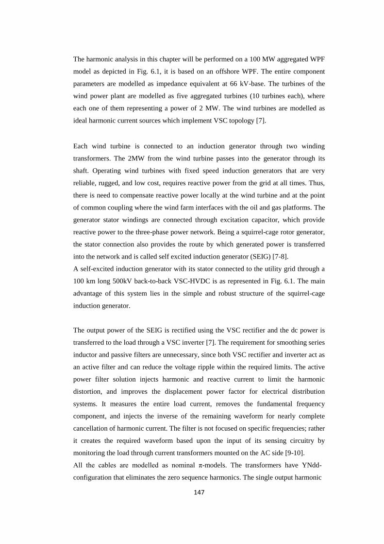
147
The harmonic analysis in this chapter will be performed on a 100 MW aggregated WPF
model as depicted in Fig. 6.1, it is based on an offshore WPF. The entire component
parameters are modelled as impedance equivalent at 66 kV-base. The turbines of the
wind power plant are modelled as five aggregated turbines (10 turbines each), where
each one of them representing a power of 2 MW. The wind turbines are modelled as
ideal harmonic current sources which implement VSC topology [7].
Each wind turbine is connected to an induction generator through two winding
transformers. The 2MW from the wind turbine passes into the generator through its
shaft. Operating wind turbines with fixed speed induction generators that are very
reliable, rugged, and low cost, requires reactive power from the grid at all times. Thus,
there is need to compensate reactive power locally at the wind turbine and at the point
of common coupling where the wind farm interfaces with the oil and gas platforms. The
generator stator windings are connected through excitation capacitor, which provide
reactive power to the three-phase power network. Being a squirrel-cage rotor generator,
the stator connection also provides the route by which generated power is transferred
into the network and is called self excited induction generator (SEIG) [7-8].
A self-excited induction generator with its stator connected to the utility grid through a
100 km long 500kV back-to-back VSC-HVDC is as represented in Fig. 6.1. The main
advantage of this system lies in the simple and robust structure of the squirrel-cage
induction generator.
The output power of the SEIG is rectified using the VSC rectifier and the dc power is
transferred to the load through a VSC inverter [7]. The requirement for smoothing series
inductor and passive filters are unnecessary, since both VSC rectifier and inverter act as
an active filter and can reduce the voltage ripple within the required limits. The active
power filter solution injects harmonic and reactive current to limit the harmonic
distortion, and improves the displacement power factor for electrical distribution
systems. It measures the entire load current, removes the fundamental frequency
component, and injects the inverse of the remaining waveform for nearly complete
cancellation of harmonic current. The filter is not focused on specific frequencies; rather
it creates the required waveform based upon the input of its sensing circuitry by
monitoring the load through current transformers mounted on the AC side [9-10].
All the cables are modelled as nominal π-models. The transformers have YNdd-
configuration that eliminates the zero sequence harmonics. The single output harmonic

148
mitigating isolation transformer is modelled as inductances to reduce the voltage
distortion created by the 3rd
and other triplen harmonic currents. That is, 3rd
, 9th and
15th harmonics and other zero sequence currents shall be treated within the secondary
windings through cancellation of the zero sequence fluxes. For 5th, 7
th, 11
th, 17
th and
19th harmonics, provided an appropriate phase shift transformer is in place, these
harmonics can be cancelled with those of other loads fed from the same primary
supply.
When determining the harmonic impedances of an oil and gas field network, or
performing harmonic penetration studies from a given harmonic current injections, the
transformers are rarely represented as harmonic sources, i.e. their inherent
magnetisation non-linearity is ignored on the assumption that the transformers have
been designed to operate within the linear region of the magnetising characteristics
[11-12]. Such an assumption may have been reasonable in earlier less competitive
times. Recent transformer designs tend to operate very close to the limit of the linear
characteristics and, even under small over-excitation; their contribution to the
harmonic content cannot be ignored [13].
In the event of determining the network harmonic admittances the transformers and
induction generators may be modelled as series impedances (i.e. series combination of
resistance and inductive). In such a case, a frequency dependent multiplying factor can
be required at the reactance sides to account for skin effect [6].
Induction motors constitute 50% of the platform loads, some are driven by variable
frequency drive (VFD). The motor is modelled as series impedances, with the
magnetizing impedance ignored. This motor type is selected due to its simple
maintenance and robustness to industrial operations. Since the motor is supplied from a
source of harmonic voltages the impedance elements in the circuit need to be modified
to account for the frequency of each harmonic that is present. The triplen harmonics can
be ignored because the motor has a star-wound stator winding, therefore only non-
triplen harmonics are considered [14-16].
The network analysis of Fig. 6.1 can be performed using the per unit (p.u) method. This
technique is selected because it is a strong tool for systems studies where several
different voltage levels exist. The impedances of the electric apparatus are usually given
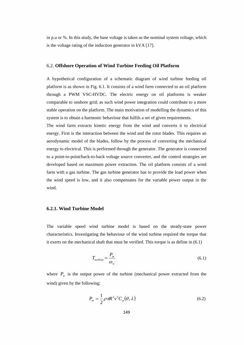
149
in p.u or %. In this study, the base voltage is taken as the nominal system voltage, which
is the voltage rating of the induction generator in kVA [17].
6.2. Offshore Operation of Wind Turbine Feeding Oil Platform
A hypothetical configuration of a schematic diagram of wind turbine feeding oil
platform is as shown in Fig. 6.1. It consists of a wind farm connected to an oil platform
through a PWM VSC-HVDC. The electric energy on oil platforms is weaker
comparable to onshore grid; as such wind power integration could contribute to a more
stable operation on the platform. The main motivation of modelling the dynamics of this
system is to obtain a harmonic behaviour that fulfils a set of given requirements.
The wind farm extracts kinetic energy from the wind and converts it to electrical
energy. First is the interaction between the wind and the rotor blades. This requires an
aerodynamic model of the blades, follow by the process of converting the mechanical
energy to electrical. This is performed through the generator. The generator is connected
to a point-to-point/back-to-back voltage source converter, and the control strategies are
developed based on maximum power extraction. The oil platform consists of a wind
farm with a gas turbine. The gas turbine generator has to provide the load power when
the wind speed is low, and it also compensates for the variable power output in the
wind.
6.2.1. Wind Turbine Model
The variable speed wind turbine model is based on the steady-state power
characteristics. Investigating the behaviour of the wind turbine required the torque that
it exerts on the mechanical shaft that must be verified. This torque is as define in (6.1)
w
m
turbine
PT
(6.1)
where wP is the output power of the turbine (mechanical power extracted from the
wind) given by the following:
,2
1 32
pm CvRP (6.2)

150
Where Pm is the mechanical output power of the wind turbine (Watt), is the Air
density (Kg/m3) = 1.29kg/m3, R is the blade radius (m) , Cp is the power coefficient of
the wind turbine and υ is the wind speed (m/second). Consequently, the output energy is
determined by the power coefficient (Cp) of wind turbine if the swept area, air density,
and wind speed are assumed to be constant. is the tip speed ratio (the rotor blade tip
speed to wind speed). Cp is function in tip speed ratio (λ) and pitch angle ( ) in degree.
If is equal zero, in this case Cp is only function in as shown in (6.2), and λ is
function of rotor mechanical speed, rotor radius of blade and wind speed as indicated in
(6.4).
Mechanical speed of the turbine w (rad/sec) is define as
R
vw
(6.3)
The power coefficient Cp characteristics of different values of the pitch angle are
illustrated Fig. 6.2 below. It should be note here that the maximum value of the
performance coefficient Cp (Cp-max = 0.48) is achieved for blade pitch angle = 0o and
for a tip-speed ratio value max = 8.0. This value is defined as the nominal value. The
power coefficient expression, based on the modelling wind turbine characteristics is
obtained using a generic equation given by
1
6
5
14.2
43
1
21),(
c
p ecccc
cC
(6.4)
where
1
003.0
02.0
113
1
The theoretical limit for CP is 0.59 according to Betz's Law, but its practical range of
variation is 0.2-0.5. [18-21]

151
0 5 10 15 200
0.1
0.2
0.3
0.4
0.5
Pow
er
Coeff
icent
(Cp)
1 = 0
2 = 5
3 = 10
4 = 15
5 = 20
6 = 25
Figure 6.2. Wind generator power curves at various wind speed
Figure 6.2 indicates the mechanical power generated by the turbine as a function of
rotor speeds for different wind speeds. The maximum power extraction within the
allowable range can be achieved if the controller can properly follow the optimum curve
with variation of wind speed. The generator side converter (a single switch three phase
mode rectifier) is controlled to extract maximum power from available wind turbine
power. Hence, the wind turbine can produce maximum power when the turbine operates
at an optimum value of Cp (Cp-opt). So it is necessary to adjust the rotor speed at
optimum value of the tip speed ratio (λopt).
The wind turbine power curves for various wind speeds can be obtained as
3
max wkP (6.5)
where
3
max
max5
2
1
PC
Rk

152
0 0.2 0.4 0.6 0.8 10
0.2
0.4
0.6
0.8
1
1.2
Wind
Tur
bine P
ower
Generator Speed
v1 = 8
v2 = 10
v3 = 12
v4 = 14
v5 = 16
v6 = 18
v7 = 20
Figure 6.3. Wind turbine rotor mechanical power
Thus knowing the wind speed, the angular speed of the wind turbine and the blade pitch
angle, then the wind turbine rotor mechanical power can be easily computed as shown
in Fig. 6.3.
Therefore, wind turbine data can be represented as follows:
Number of blades = 3
Blade radius (m) = 24
Nominal rotational speed Nm = 25 rpm
Air density (kg/m3) = 1.29kg/m
3
Optimal lambda ( ) = 8.0
Performance coefficient Cp = 0.48
Selecting the operating speed of the generator and controlling it with changing wind
speed must be determined early in the system design. This is important, as it determines
all major components and their ratings. The alternative strategies and the corresponding
speed control methods fall in the following categories. That is fixed-speed drive and
variable-speed using power electronics.
The fixed-speed operation of the generator naturally fits well with the induction
generator, which is inherently a fixed-speed machine. But, the turbine speed is generally
low, while the electrical generator works effectively at high speed. Thus, the equal
speed between the two is obtained through a mechanical gearbox. The gearbox
decreases the speed and increases the torque, thereby improving the rotor power
coefficient CP.

153
The major disadvantage of fixed-speed is that it almost never captures the wind energy
at the peak efficiency in terms of the rotor power coefficient CP. The wind energy is
wasted when the wind speed is higher or lower than the certain value selected as the
optimum. The two-speed machine increases the energy capture, reduces the electrical
loss in the rotor and reduces the gear noise. The speed is change by changing the gear
ratio. A gear ratio is the relationship between the numbers of teeth on two or more gears
that are meshed [22]. The turbine torque varies with the gear ratio and the turbine wind
velocity as depicts in Fig. 6.4.
1 2 3 4 5 6 7 8-10
-5
0
5
10
15
20
Turbine wind velocity (m/s)
Turb
ine t
orq
ue
Figure 6.4 speed characteristic of wind turbine with low and high gear ratios.
The system is operated on the low-gear ratio for wind speed below 4 m/s and on the
high-gear ratio for wind speed above 4 m/s. The gear ratio is changed at 4 m/s, the
generator however operates with only one-speed ratio of 100:1. Self-excitation can
occur in a fixed-speed wind turbine equipped with an induction generator. Fixed
capacitors supplies reactive power compensation in a fixed-speed wind turbine.
Induction generators alone cannot self excite. It requires reactive power from the grid to
operate normally. The grid dictates the voltage and frequency of the induction
generator.
When the generator reaches its rated power, the turbines must limit the magnitude of
mechanical power delivered to the generator. As shown in Fig. 6.4, the generator
reaches its rated power at wind speeds of 3 m/s to 6 m/s, and thus, must decrease in
energy collection at higher wind speeds. This energy collection control is achieved by
either stall, pitch, or a combination of them both, called active stall. There are no
moving parts in stall-controlled blades, and the challenge in this control technique is
proper blade construction to avoid vibration and permit a gradual stalling. The pitch

154
function provides full control over the mechanical power. The pitch angle is controlled
to keep the generator at the rated power by reducing the angle of the blades. By
actuating the blade angle to be at the limit of the stalling, fast torque changes in the
wind speed can be tolerated [23-24].
6.3. Induction Generator Modelling for Offshore Wind Turbine
The invention of induction generators completed the ac system of electrical power
production, transmission, and utilization. Induction generators require no electrical
connection to the rotor windings. Instead, the rotor winding are short-circuited. The
magnetic flux flowing across the air gap links these closed rotor circuits.
The stator of the induction generators (IGs) is made of numerous coils with three
phases, and is supplied with three phase current. The three coils are physically
distributed around the stator area with out of time-phase currents, which produces a
rotating magnetic field. Induction generators are asynchronous speed machines,
operating speed is slightly less than synchronous speed in the motor mode and slightly
greater than synchronous speed in the generator mode. Induction machines are
sometimes operated in the motor mode, so they are usually called induction motors [25-
26].
Induction generators have relatively advantageous features over conventional
synchronous generators. These features are brushless and rugged construction, low cost,
maintenance and operational simplicity, self-protection against faults, and good
dynamic response. Induction generators have the capability of generating power at
varying speed; this facilitates the induction generator operation in a stand-alone or
isolated mode to supply remote areas where grid extension is not economically viable,
in conjunction with the synchronous generator to fulfil the increased local power
demand of the grid by integrating power from resources located at different sites. The
disadvantage found in induction generator is the reactive power requirement. The
reactive power can be supplied from the grid and capacitor compensator [27-34].
6.3.1. SEIG with External Capacitor
Since the excitation current is mainly reactive, a stand-alone system is self-excited by
shunt capacitors. In grid-connected operation, it draws excitation power from the

155
network, and its output frequency and voltage values are dictated by the grid. Where the
grid capacity of supplying the reactive power is limited, local capacitors can be used to
partly supply the needed reactive power [35-40].
Self-excited induction generator (SEIG) works in the saturation region and it has
excitation capacitors connected across its stator terminals as shown in Fig. 6.5. These
generators are an ideal choice for electricity generation in stand-alone variable speed
wind energy systems, where reactive power from the grid is not available. The induction
generator will self-excite, using the external capacitor, only if the rotor has an adequate
remnant magnetic field. In the self-excited mode, the generator output frequency and
voltage are affected by the speed, the load, and the capacitance value in Farads [41-42].
Figure 6.5. Self-excited induction generator with external capacitor.
Steady-state analysis of induction generators is of interest both from the design and
operational points of view. Knowing the parameters of the machine, it is possible to
determine the performance of the machine at a given speed, capacitance and load
conditions.
Loop impedance and nodal admittance methods used for the analysis of SEIG are both
based on per phase steady-state equivalent circuit of the induction machine as
represented in Fig. 6.5, modified for the self-excitation case. This structure is very
effective in calculating the minimum value of capacitance needed for guaranteeing self-
excitation of the induction generator. For stable operation, the excitation capacitance
must be slightly higher than the minimum value. Also there is a speed threshold, below
which no excitation is possible, i.e.
the cutoff speed of the machine [43-45].
LOAD cx mx
mr
~
2I
0I
'
2
1r
s
s
21 xx
21 rr
~
1I ~
1V

156
The mutual inductance MX is related to the voltage
F
Vgacross it by the following
equation
2
1
K
F
VK
X
g
M
(6.6)
L
SL
TgZ
ZZVV (6.7)
where
1K and 2K depend on the design of the machine
The capacitors compensators of the wind turbine are switched capacitors. Manufacturer
usually set the wind turbine with only a few hundred kVAR for reactive power
compensation. The wind turbine is compensated at different levels of compensation
depending on the level of generation. In the event of losses in the capacitor, a resistor
may be included in series with the capacitance. The losses in the capacitors are usually
very small for high quality capacitors [46].
Figure 6.6. Equivalent circuit of self-excited induction generator with R-L Load.
where
Rs, Rr, R : p.u. per-phase stator, rotor (referred to stator) and load resistance
respectively.
Xls, Xlr, X, Xm : p.u. per-phase stator leakage, rotor leakage (referred to stator), load and
magnetizing reactances (at base frequency), respectively.
Xsmax : p.u. maximum saturated magnetizing reactance.
C : per-phase terminal-excitation capacitance.
CI LI RI sI
FVT /
RjhX
SjhX
RL
Load
2/ FjhX c
mjhx
FRS /
vF
RR
1E
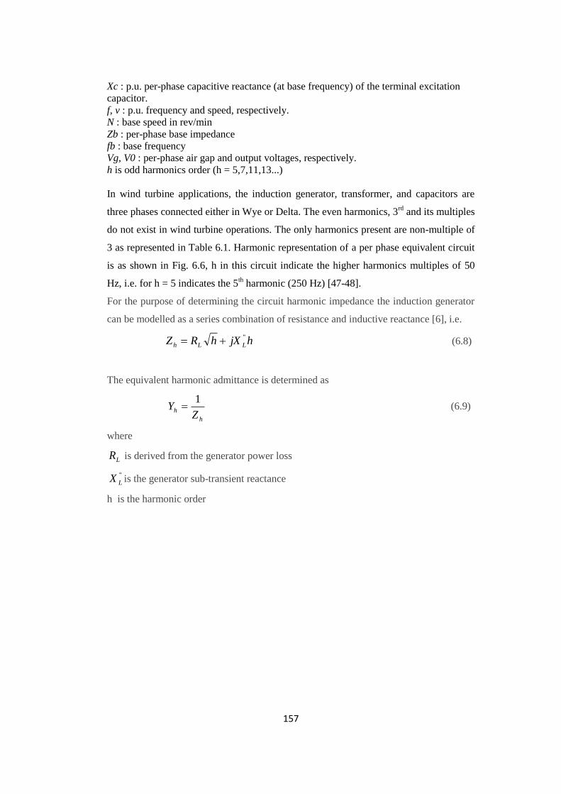
157
Xc : p.u. per-phase capacitive reactance (at base frequency) of the terminal excitation
capacitor.
f, v : p.u. frequency and speed, respectively.
N : base speed in rev/min
Zb : per-phase base impedance
fb : base frequency
Vg, V0 : per-phase air gap and output voltages, respectively.
h is odd harmonics order (h = 5,7,11,13...)
In wind turbine applications, the induction generator, transformer, and capacitors are
three phases connected either in Wye or Delta. The even harmonics, 3rd
and its multiples
do not exist in wind turbine operations. The only harmonics present are non-multiple of
3 as represented in Table 6.1. Harmonic representation of a per phase equivalent circuit
is as shown in Fig. 6.6, h in this circuit indicate the higher harmonics multiples of 50
Hz, i.e. for h = 5 indicates the 5th harmonic (250 Hz) [47-48].
For the purpose of determining the circuit harmonic impedance the induction generator
can be modelled as a series combination of resistance and inductive reactance [6], i.e.
hjXhRZ LLh
'' (6.8)
The equivalent harmonic admittance is determined as
h
hZ
Y1
(6.9)
where
LR is derived from the generator power loss
''
LX is the generator sub-transient reactance
h is the harmonic order
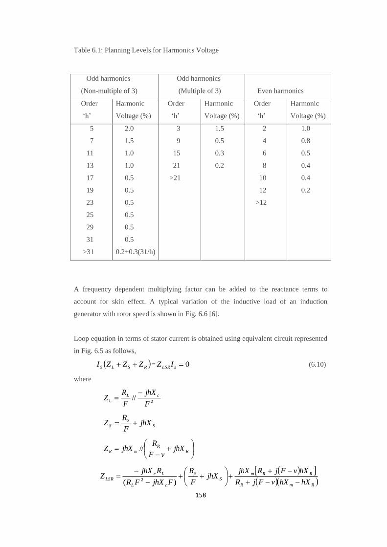
158
Table 6.1: Planning Levels for Harmonics Voltage
Odd harmonics
(Non-multiple of 3)
Odd harmonics
(Multiple of 3)
Even harmonics
Order
‘h’
Harmonic
Voltage (%)
Order
‘h’
Harmonic
Voltage (%)
Order
‘h’
Harmonic
Voltage (%)
5
7
11
13
17
19
23
25
29
31
>31
2.0
1.5
1.0
1.0
0.5
0.5
0.5
0.5
0.5
0.5
0.2+0.3(31/h)
3
9
15
21
>21
1.5
0.5
0.3
0.2
2
4
6
8
10
12
>12
1.0
0.8
0.5
0.4
0.4
0.2
A frequency dependent multiplying factor can be added to the reactance terms to
account for skin effect. A typical variation of the inductive load of an induction
generator with rotor speed is shown in Fig. 6.6 [6].
Loop equation in terms of stator current is obtained using equivalent circuit represented
in Fig. 6.5 as follows,
RSLS ZZZI = 0sLSRIZ (6.10)
where
2
//F
jhX
F
RZ cL
L
S
S
S jhXF
RZ
R
RmR jhX
vF
RjhXZ //
RmR
RRm
S
S
cL
Lc
LSRhXhXvFjR
hXvFjRjhXjhX
F
R
FjhXFR
RjhXZ
)( 2

159
(6.11)
where
2
2
max
11
11
2
m
r
r
s
c
X
X
R
R
v
v
vvF is the self-excited frequency
2
12
m
r
s
r
m
s
cX
X
R
R
X
Rv
v is the rotor speed sr s 1
Under steady state operation of SEIG, SI 0 , therefore
The value of stator current is
SL
g
SZZ
F
V
I
(6.12)
The value of the rotor current
R
R
g
R
jhXvF
R
F
V
I (6.13)
The value of the load current
CL
SC
LjhXFR
IjhXI
(6.14)
The value of the terminal voltage
LLT RIV (6.15)
The value of the output power
vF
FRIP
RR
in
2
(6.16)
LLout RIP2
(6.17)
0LSRZ (6.18)
In appeandix A4, Equ. (A4.21) has real and imaginary parts as follows
Re LSRZ = 0

160
Im LSRZ = 0 (6.19)
In stable operating condition of an SEIG, (6.13) and (6.19) must be satisfied.
Equation (6.16) and (6.19) may be solved using optimization technique to determine the
excitation capacitance and generated frequency for the desired terminal voltage.
The operations of the real part can be obtained as
001
2
2
3
3
4
4 CFCFCFCFC (6.20)
where
220 IvRRRRRC rSLSL
321
2
2321
2
1 22 IIIvRRRRRvIRRIIIvRRC rSLSLSLrL
2
2
2
3
222
1
132
2
2
2
321
2
2
2
2 2
IRIRvIR
IIIRRRvIRRhXIIRIRIRRC
SrL
SrLrSLrrSL
vIRIRhXIIIvRhXC LSLrL
2
1
2
2
22
321
2
3 2
2
1
2
2
2
132
2
4 IRIRXIIIRXC LSLrL
hXXhXXhXI MRMRS 1
MR hXXI 2
SM XXhI 3
h harmonic of the order of 5,7,11,13,17,19,23,25,...
Its imaginary part contains information for maximum value of terminal capacitor and is
obtained as follows
2
2
2
1
4
3
max2
1
YY
Y
Y
FXC L
(6.21)
where
vFFIRRY rS 11
232 IvFRFIRY Sr
23 FhXRY LL
vFFYIYRY r 1224

161
6.3.2. Test Case Impact of Harmonic Injection Stabilizer and Capacitor
Excitation
It should be reiterated here that (6.20) contained four possible real roots that ignite self-
excitation and it has only physical meaning. The Fig. 6.7 to Fig. 6.14 illustrates the
impact of harmonic injection stabilizer and capacitor excitation to stabilize an induction
generator in a wind turbine. As shown in Fig. 6.7 is injection of 5th harmonic at fixed
resistive load with variable inductive load, as observed capacitor self-excitation occurs
between 50% and 100% inductive load. There is under excitation when inductive load is
0%, hence the capacitance collapses after hitting its maximum.
500 1000 1500 2000 2500 3000 3500
0
50
100
150
200
250
Max
imum
Cap
acita
nce
(uF)
Speed (rpm)
XL=0%
XL=50%
XL=100%
XL=200%
Figure 6.7. Maximum capacitance at 5th harmonic
A large variation in the capacitor profile is recorded when the value of the inductive
load is increased from an initial value 0% to 50%. The 50% and 100% values stabilize
at maximum capacitance excitation of 170 μF with 100% value recording overshoot of
5μF. The 200% recorded lower settling value of 152μF but have high overshoot
capacitor value of 30 μF.
500 1000 1500 2000 2500 3000 35000
100
200
300
400
Min
imum
Fre
quen
cy (H
z)
Speed (rpm)
XL=0%
XL=50%
XL=100%
XL=200%
Figure 6.8. Exciter load-saturation curve at 5th harmonic
250Hz
5th harmonics
Air gap line
Fixed Resistance load
Saturation curve
Operating point
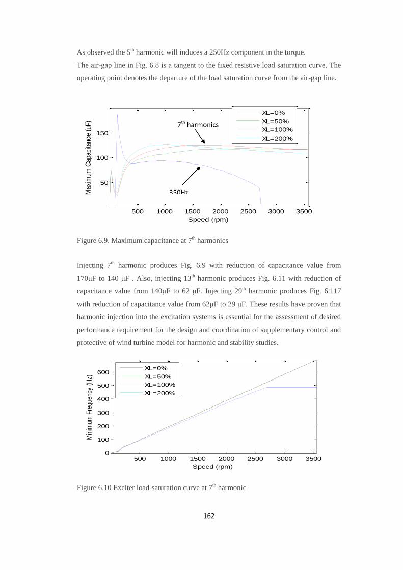
162
As observed the 5th harmonic will induces a 250Hz component in the torque.
The air-gap line in Fig. 6.8 is a tangent to the fixed resistive load saturation curve. The
operating point denotes the departure of the load saturation curve from the air-gap line.
500 1000 1500 2000 2500 3000 3500
50
100
150
Max
imum
Cap
acita
nce
(uF
)
Speed (rpm)
XL=0%
XL=50%
XL=100%
XL=200%
Figure 6.9. Maximum capacitance at 7th harmonics
Injecting 7th harmonic produces Fig. 6.9 with reduction of capacitance value from
170μF to 140 μF . Also, injecting 13th harmonic produces Fig. 6.11 with reduction of
capacitance value from 140μF to 62 μF. Injecting 29th harmonic produces Fig. 6.117
with reduction of capacitance value from 62μF to 29 μF. These results have proven that
harmonic injection into the excitation systems is essential for the assessment of desired
performance requirement for the design and coordination of supplementary control and
protective of wind turbine model for harmonic and stability studies.
500 1000 1500 2000 2500 3000 35000
100
200
300
400
500
600
Min
imum
Fre
quen
cy (
Hz)
Speed (rpm)
XL=0%
XL=50%
XL=100%
XL=200%
Figure 6.10 Exciter load-saturation curve at 7th harmonic
350Hz
7th harmonics

163
500 1000 1500 2000 2500 3000 35000
20
40
60
80
100
Max
imum
Cap
acita
nce
(uF
)
Speed (rpm)
XL=0%
XL=50%
XL=100%
XL=200%
Figure 6.11 Maximum capacitance at 13th harmonic
500 1000 1500 2000 2500 3000 35000
200
400
600
800
1000
1200
Min
imum
Fre
quen
cy (
Hz)
Speed (rpm)
XL=0%
XL=50%
XL=100%
XL=200%
Figure 6.12 Exciter load-saturation curve at 13th harmonic
500 1000 1500 2000 2500 3000 35000
10
20
30
40
Max
imum
Cap
acita
nce
(uF
)
Speed (rpm)
XL=0%
XL=50%
XL=100%
XL=200%
Figure 6.13. Maximum capacitance at 29th harmonic
1450Hz
29th harmonics
650Hz
13th harmonics

164
500 1000 1500 2000 2500 3000 3500
0
500
1000
1500
2000
2500
Min
imum
Fre
quen
cy (H
z)
Speed (rpm)
XL=0%
XL=50%
XL=100%
XL=200%
Figure 6.14. Exciter load-saturation curve at 29th harmonic
Injection of high odd harmonics as shown in Fig. 6.13 generates low capacitance value.
When the capacitance is large it takes a longer time to reach its steady state value. If the
capacitance is too small there will not be enough exciting current and as a result there
will not be voltage build up. As observed in the figures under considerations the
inductive load must be kept low to achieve stabilized capacitance value, since large
inductive load will introduce unstable behaviour.
Examining these figures reveals the following remarks:
For all harmonics components, gives good estimates for the capacitance
magnitudes due to odd harmonic injection.
As the non-multiple of 3rd
harmonics increases, relatively low capacitance
magnitudes are achieved.
At a low non-multiple of 3rd
harmonics, the simulation produces high
magnitude.
The critical capacitance value is 10 μF of the initial region of capacitor curve. If
the capacitance is chosen below the critical capacitance 10 μF, the voltages will
never build-up and excitation fails initially.
The minimum capacitance required to generate the rated voltage is 28 μF. If we
choose below this value, the rated voltage will not be generated.
The maximum value of capacitance required should not exceed 30 μF. If the
capacitance exceeds the maximum value, the current flow will be more than the
rated value. This may lead to heating of stator core.
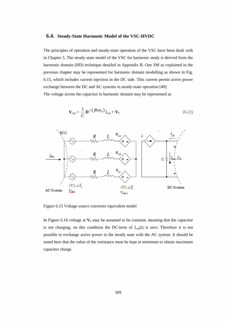
165
6.4. Steady-State Harmonic Model of the VSC-HVDC
The principles of operation and steady-state operation of the VSC have been dealt with
in Chapter 5. The steady-state model of the VSC for harmonic study is derived from the
harmonic domain (HD) technique detailed in Appendix B. One SM as explained in the
previous chapter may be represented for harmonic domain modelling as shown in Fig.
6.15, which includes current injection in the DC side. This current permit active power
exchange between the DC and AC systems in steady-state operation [49].
The voltage across the capacitor in harmonic domain may be represented as
Vcap = C
1D
-1 )( 0jhIcap + V0 (6.22)
Figure 6.15 Voltage source converter equivalent model
In Figure 6.16 voltage at V0 may be assumed to be constant, meaning that the capacitor
is not charging, on this condition the DC-term of Icap(t) is zero. Therefore it is not
possible to exchange active power in the steady state with the AC system. It should be
noted here that the value of the resistance must be kept at minimum to obtain maximum
capacitor charge.

166
0 0.2 0.4 0.6 0.8 1
0
1
2
3
4
5
Time, s
Volta
ge, V
Capacitor
DischargingCapacitor Charging
Figure 6.16 shows the charging and discharging curves
Maintaining the required DC capacitor voltage has to correspond to the active power
supplied by the DC side. This has to be equal to the active power absorbed by the AC
side with the losses of the VSC, which include the switching losses and capacitor losses
in the converter.
0 0.01 0.02 0.03 0.04 0.05-60
-40
-20
0
20
v(t), V
i(t), A
Capacitor-charging
Time
Magnitude
Figure 6.17. Voltage and current of DC capacitor
On any scenario that the active power is greater than the AC side will result in converter
losses, the excess quantity will be absorbed by the VSC resulting in DC capacitor
voltage increase. In the reverse, if the active power is less than the AC side requirement
with the converter losses, the DC capacitor voltage will decrease as shown in Fig. 6.17.
V0
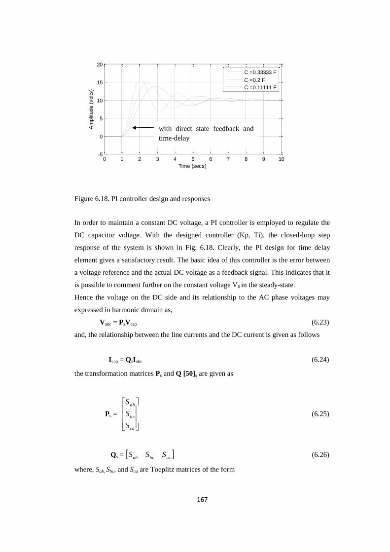
167
0 1 2 3 4 5 6 7 8 9 10-5
0
5
10
15
20
Time (secs)
Am
plit
ude (
volts)
C =0.33333 F
C =0.2 F
C =0.11111 F
Figure 6.18. PI controller design and responses
In order to maintain a constant DC voltage, a PI controller is employed to regulate the
DC capacitor voltage. With the designed controller (Kp, Ti), the closed-loop step
response of the system is shown in Fig. 6.18. Clearly, the PI design for time delay
element gives a satisfactory result. The basic idea of this controller is the error between
a voltage reference and the actual DC voltage as a feedback signal. This indicates that it
is possible to comment further on the constant voltage V0 in the steady-state.
Hence the voltage on the DC side and its relationship to the AC phase voltages may
expressed in harmonic domain as,
Vabc = PsVcap (6.23)
and, the relationship between the line currents and the DC current is given as follows
Icap = QsIabc (6.24)
the transformation matrices Ps and Q [50]s are given as
Ps =
ca
bc
ab
S
S
S
(6.25)
Qs = cabcab SSS (6.26)
where, Sab, Sbc, and Sca are Toeplitz matrices of the form
with direct state feedback and
time-delay
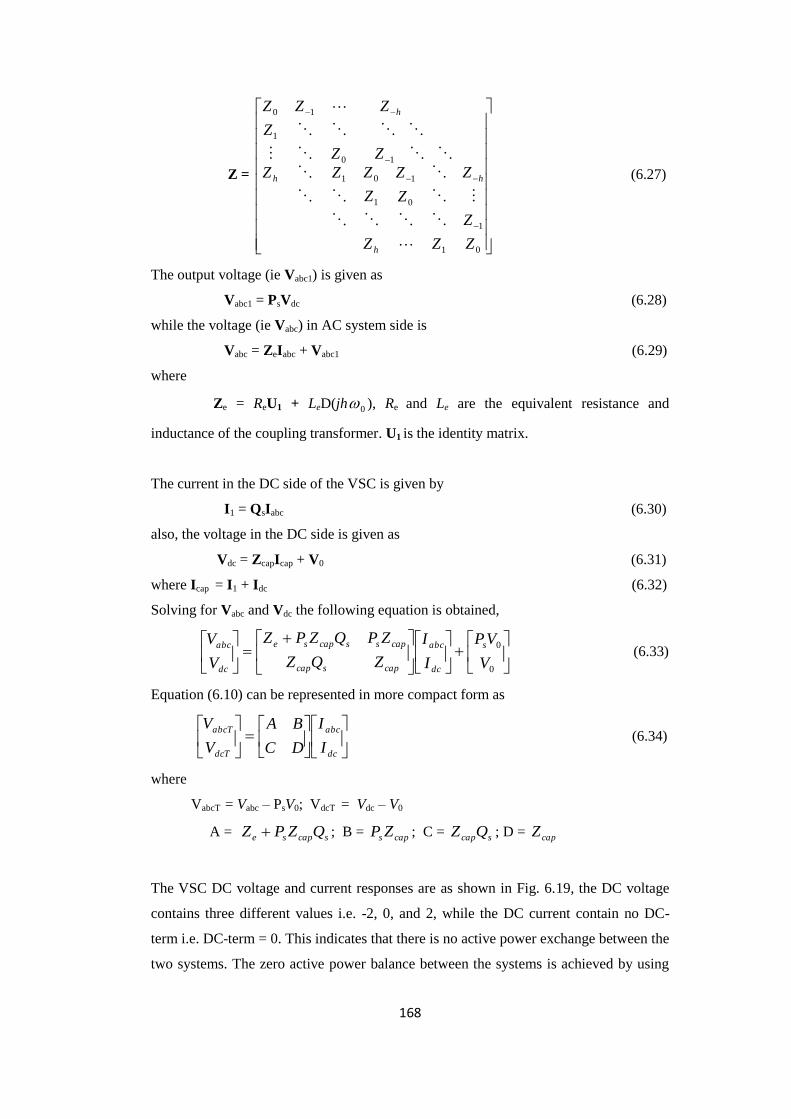
168
Z =
0
1
1
0
1
1
01
10
1
10
Z
Z
Z
Z
Z
Z
Z
Z
ZZZ
ZZ
Z
ZZZ
h
h
h
h
(6.27)
The output voltage (ie Vabc1) is given as
Vabc1 = PsVdc (6.28)
while the voltage (ie Vabc) in AC system side is
Vabc = ZeIabc + Vabc1 (6.29)
where
Ze = ReU1 + LeD(jh 0 ), Re and Le are the equivalent resistance and
inductance of the coupling transformer. U1 is the identity matrix.
The current in the DC side of the VSC is given by
I1 = QsIabc (6.30)
also, the voltage in the DC side is given as
Vdc = ZcapIcap + V0 (6.31)
where Icap = I1 + Idc (6.32)
Solving for Vabc and Vdc the following equation is obtained,
0
0
V
VP
I
I
ZQZ
ZPQZPZ
V
V s
dc
abc
capscap
capsscapse
dc
abc (6.33)
Equation (6.10) can be represented in more compact form as
dc
abc
dcT
abcT
I
I
DC
BA
V
V (6.34)
where
VabcT = Vabc – PsV0; VdcT = Vdc – V0
A = scapse QZPZ ; B = caps ZP ; C = scapQZ ; D = capZ
The VSC DC voltage and current responses are as shown in Fig. 6.19, the DC voltage
contains three different values i.e. -2, 0, and 2, while the DC current contain no DC-
term i.e. DC-term = 0. This indicates that there is no active power exchange between the
two systems. The zero active power balance between the systems is achieved by using

169
proper phase shift angle of the PWM modulation signal resulting in a VSC DC voltage
output. This condition gives a 120o phase shift angle of ia(t) with respect to the voltage.
20 40 60 80 100 120 140 160-2
0
2
x 104 Vdc
20 40 60 80 100 120 140 160-3
-2
-1
0
x 104
Frequency(Hz)
Magnitude
Idc
Figure 6.19. Voltage and current in the DC side
The frequency content of the DC voltage signal is as shown in Fig. 6.20 and its complex
conjugate is as represented in Fig. 6.21, which determine the real harmonic magnitude
in the DC voltage signal. As observed in the harmonic spectrum, one dominant
harmonic content appears which has no significant effect in the DC voltage signal.
The Fast Fourier Transform (FFT) of Fig. 6.19 (i.e Vdc) is represented in Fig. 6.20 and
real part of this signal is as shown in Fig. 6.21. The FFT algorithm applied here
comprises a number of elements which is equal to 2n (e.g. 2
8 = 256, 2
10 = 1024 etc). Its
main advantage is that it significantly reduces the computational time by a factor of the
order n/log2n, i.e. more than 100 times for a sample of 1024 elements.
The number of FFT elements is equal to the size of the time sample which contains
complex conjugates and does not carry any new information. All the components of the
harmonic spectrum produce the correct estimate of the voltage magnitude of Fig. 6.19.
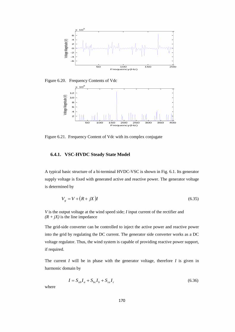
170
50 100 150 200
-6
-4
-2
0
2
4
6
x 105
Frequency(Hz)
Volta
ge M
agnit
ude (
V)
Figure 6.20. Frequency Contents of Vdc
50 100 150 200 250 300 350 400
2
4
6
8
10
12
x 108
Frequency(Hz)
Volta
ge M
agnit
ude (
V)
Figure 6.21. Frequency Content of Vdc with its complex conjugate
6.4.1. VSC-HVDC Steady State Model
A typical basic structure of a bi-terminal HVDC-VSC is shown in Fig. 6.1. Its generator
supply voltage is fixed with generated active and reactive power. The generator voltage
is determined by
IjXRVVg (6.35)
V is the output voltage at the wind speed side; I input current of the rectifier and
(R + jX) is the line impedance
The grid-side converter can be controlled to inject the active power and reactive power
into the grid by regulating the DC current. The generator side converter works as a DC
voltage regulator. Thus, the wind system is capable of providing reactive power support,
if required.
The current I will be in phase with the generator voltage, therefore I is given in
harmonic domain by
ccabbcaab ISISISI (6.36)
where

171
Sab, Sbc and Sca are Phase switching function
Ia, Ib and Ic are line currents
50 100 150 200 250 300
-1000
-500
0
500
1000C
urr
ent
Magnitude
Frequency(Hz)
Converter input current (Iin)
50 100 150 200 250 300 350 400
-1000
-500
0
500
1000
Cur
rent
Mag
nitu
de
Frequency(Hz)
Converter input current (Iin2)
Figure 6.22. Input current of the (a) rectifier and (b) inverter
10 20 30 40 50 60
-2
0
2
4
6
x 109
Frequency (Hz)
Voltage M
agnitude
vc1
vc2
Figure 6.23. Output voltage of wind speed side and AC output voltage of the
platform side
(a)
(b)
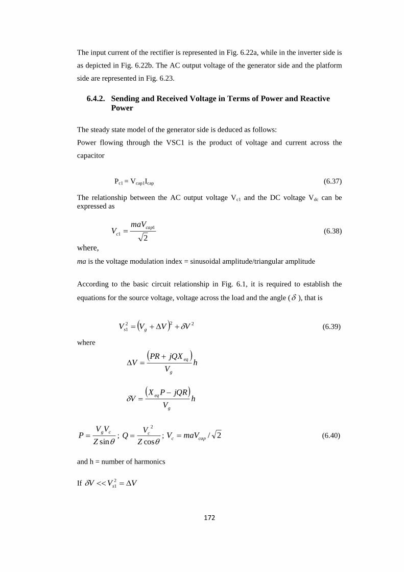
172
The input current of the rectifier is represented in Fig. 6.22a, while in the inverter side is
as depicted in Fig. 6.22b. The AC output voltage of the generator side and the platform
side are represented in Fig. 6.23.
6.4.2. Sending and Received Voltage in Terms of Power and Reactive
Power
The steady state model of the generator side is deduced as follows:
Power flowing through the VSC1 is the product of voltage and current across the
capacitor
Pc1 = Vcap1Icap (6.37)
The relationship between the AC output voltage Vc1 and the DC voltage Vdc can be
expressed as
2
1
1
cap
c
maVV (6.38)
where,
ma is the voltage modulation index = sinusoidal amplitude/triangular amplitude
According to the basic circuit relationship in Fig. 6.1, it is required to establish the
equations for the source voltage, voltage across the load and the angle ( ), that is
222
1 VVVV gs (6.39)
where
hV
jQXPRV
g
eq
hV
jQRPXV
g
eq
sinZ
VVP
cg ;
cos
2
Z
VQ c ; 2/capc maVV (6.40)
and h = number of harmonics
If VVV s 2
1

173
2
2
1
g
gscV
jQXRPVV (6.42)
Also, if 0R
therefore, g
gscV
jQXVV 2
Thus, voltage depends only on Q, if and only QXVPX c 2
1 , and angle of
transmission is obtained from 2
1
1sinscV
V which only depend on P
The load angle control can be determine using power transfer, active power P and
reactive power Q between the sending and receiving end of Fig. 6.1. The quantities S
(volt-amperes), known as the complex power, may be obtained by product of Vc1 and
the conjugate of current (I) [51]. Assuming that
*
21
1
*
1
Z
VVVIVS cc
ccG (6.43)
=
j
c
j
cj
cZe
VeVeV 21
1 (6.44)
= jccjc e
Z
VVe
Z
V 21
2
1 (6.45)
PVSC1 = coscos 21
2
1
Z
VV
Z
V ccc MW (6.46)
QVSC1 = sinsin 21
2
1
Z
VV
Z
V ccc Mvar (6.47)
Similarly,
=
j
j
c
cZe
VeVV 2
2 (6.48)
PVSC2 = coscos 21
2
2
Z
VV
Z
V ccc MW (6.49)
QVSC2 = sinsin 21
2
2
Z
VV
Z
V ccc Mvar (6.50)

174
The active and reactive powers in VSC1 and VSC2 with dc link impedance (DC
resistance) are as shown in Fig. 6.24. Also, the active and reactive powers in VSC1 and
VSC2 sides without dc link impedance are as represented in Fig. 6.25. As observed the
system with a dc link has low active and reactive power magnitude, comparable to the
system without dc link which higher magnitude as shown in Fig. 6.25.
10 20 30 40 50 60
-4
-2
0
2
x 1019
Frequency (Hz)
Magnitude
Pac1
Qac1
Pac2
Qac2
Figure 6.24. Active and reactive power of VSC1 and VSC2 with DC link impedance
5 10 15 20 25 30 35 40 45 50 55
-5
0
5
10
15
x 1018
Frequency (Hz)
Magnitude
Pac1
Qac1
Pac2
Qac2
Figure 6.25. Active and reactive power of VSC1 and VSC2 without DC
link impedance
The wind turbine generator and power transfer from the generator to the DC link are
controlled by adjusting the magnitude and angle of the voltage at the AC terminals of
the VSC1 side. The voltage magnitude, 1RV and angle magnitude, 1 required at the
terminals of the generator-side VSC1 are as shown in Fig 6.26 and are obtained as
follows:
1
1
11
s
gengens
sgV
XQVV (6.51)
and
11
1
1
sc
gengens
VV
XP (6.52)

175
10 20 30 40 50 60
-4
-2
0
2
4
6
x 1019
Frequency (Hz)
Magnitude
VR1
Angd1
Figure 6.26. Load angle and voltage magnitude control of the generator-side converter
Similarly,
The voltage magnitude, 2RV and angle magnitude, 2 required at the terminals of the
generator-side VSC2 are as shown in Fig 6.27 and are obtained as follows:
2
2
22
s
platformplatforms
sgV
XQVV (6.53)
and
22
2
1
sc
platformplatform
VV
XP (6.54)
10 20 30 40 50 60
0
5
10
x 1019
Frequency (Hz)
Magnitude
VR1
Angd1
Figure 6.27. Load angle and voltage magnitude control of the platform-side converter
Figure 6.31 illustrates the implementation of the load angle and voltage magnitude
control for the oil platform-side VSC2 with the reactive power exchange equal to zero
with the network (i.e. 02 platformsQ for unity power factor operation).

176
6.5. Harmonic Determination Needed in the Capacitor Bank
When harmonics appear to be the cause of the system problems, it is desirable to
determine the system harmonic resonance point. To obtain this resonance point, the
short-circuit capacity of each capacitor bank location is needed.
As it can be seen from the power distribution network Fig. 6.1, the power-factor-
correction capacitor bank, which is connected on the 11 kV bus, can create a parallel
resonance between the capacitors and the system source inductance.
To ascertain if harmonic considerations are required in the capacitor banks, the
following equations applies,
with damping
2
22/
C
L
TXC
TXs
MVA
MW
ZMVA
MVAH (6.55)
without damping TXC
TXs
ZMVA
MVAH
2/ (6.56)
where
Hs is the series resonance point
MVATX is the transformer MVA
ZTX is the transformer impedance
MWL is the damping factor
Approximate parallel resonance point may be obtain by the equation
C
SC
pMVA
MVAH (6.57)
where
Hp is the parallel resonance point at fundamental frequency
MVASC is the short circuit capacity
MVAC is the Mvar rating of the unfiltered capacitor bank at that location
The following test results show enforcement of harmonic considerations needed in the
capacitor banks. Utilizing the system data, the following test results are obtained, Fig.
6.28a depicts resonance point close to 3rd
, 5th, 7
th , 9
th and 11
th and Fig. 6.30a depicts
15th, 19
th, 23
rd, 25
th, and 29
th possible harmonic-related problem could occur. The test
results produce a solution or at least identify the cause of a harmonic problem, so that

177
the need for a detailed harmonic study is either reduced or the study is greatly simplified
in the capacitor banks..
0 1 2 3 4 5 6 7 8 9 10
-0.01
-0.005
0
0.005
0.01
Magnitude
Time(sec)
Hs = 5
0 2 4 6 8 10
-0.01
-0.005
0
0.005
0.01
Magnitude
Time(sec)
Hs = 23
0 1 2 3 4 5 6 7 8 9 10
-0.03
-0.02
-0.01
0
0.01
0.02
0.03
Magnitude
Time(sec)
Hs = 23
Figure 6.28. Series resonance harmonic point with damping in OG 1
(b)
(a)
(c)
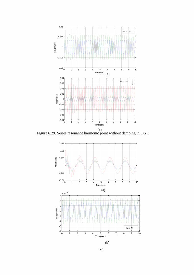
178
0 1 2 3 4 5 6 7 8 9 10
-0.01
-0.005
0
0.005
0.01
Magnitude
Time(sec)
Hs = 24
0 1 2 3 4 5 6 7 8 9 10
-0.04
-0.03
-0.02
-0.01
0
0.01
0.02
0.03
0.04
Magnitude
Time(sec)
Hs = 24
Figure 6.29. Series resonance harmonic point without damping in OG 1
0 1 2 3 4 5 6 7 8 9 10
-0.01
-0.005
0
0.005
0.01
0.015
Magnitude
Time(sec)
0 1 2 3 4 5 6 7 8 9 10
-8
-6
-4
-2
0
2
4
6x 10
-3
Magnitude
Time(sec)
Hs = 20
(a)
(b)
(a)
(b)

179
0 1 2 3 4 5 6 7 8 9 10
-0.02
-0.01
0
0.01
0.02
Magnitude
Time(sec)
Hs = 20
Figure 6.30. Series resonance harmonic point with damping in OG 2
0 1 2 3 4 5 6 7 8 9 10
-0.01
-0.005
0
0.005
0.01
Magnitude
Time(sec)
Hs = 22
0 1 2 3 4 5 6 7 8 9 10
-0.03
-0.02
-0.01
0
0.01
0.02
0.03
Magnitude
Time(sec)
Hs = 22
Figure 6.31. Series resonance harmonic point without damping in OG 2
It is uncommon to encounter a system where it is more practical to make a harmonic
study on a system model as a diagnostic measure rather than to perform a detailed, time
consuming harmonic analysis study. The results are used to obtain a harmonic spectrum
as input data by which the system model is confirmed prior to performance of a detailed
harmonic analysis study. In a way of confirmation, Fig. 6.28b, 6.28c and Fig. 6.29b,
6.29c depicts series resonance harmonic point with and without damping at PCC1
respectively. And Fig. 6.30b, 6.30c and Fig. 6.31b, 6.31c depicts series resonance
(c)
(a)
(b)

180
harmonic point with and without damping at PCC2 bus respectively. As observed no
harmonic appear that can cause system problems comparable to Fig. 6.28a and Fig.
6.30a. These suggest the right input data for capacitor banks with corresponding
transformers on the oil platform by which the system can operate without harmonic
distortion.
6.6. Harmonic Deriving Point Impedance of Oil Platform
The impedances of the components of a oil and gas system to harmonic frequencies are
determined on the basis of their values at power frequency (50 Hz or 60 Hz). The model
of components of the system is as shown in Fig. 6.1. The choice of the model depends
solely on the accuracy sought, the data and the range of operating frequencies.
It should be iterated here that, the complete system can never be represented in full in
all harmonics studies. This will mandate the use of equivalent impedance representing
its behaviour to harmonic disturbance for some components. These impedances depend
on the short-circuit power of systems, the length of cable lines, the capacitor banks for
reactive power compensation, the transformers, generating plant, the load levels of the
system and the power electronics equipment. The software simulation method can be
used to estimate these impedances.
The load on an oil and gas platform can roughly be divided in to three types of load:
direct online AC motors, variable speed drives, and passive loads. The total electric
power demand, and distribution between the different types of load, can vary greatly
depending on the design of the platform and the operations running on the platform.
The system to be modelled is a simple radial oil and gas platform network with PCC
voltage levels (11kV and 6.6 kV), fed by 100MW aggregated wind farm generators,
66kV, VSC-HVDC 500km system.
If a harmonic modelling study indicates excessive harmonic levels or a potentially
harmful resonance condition, there are a number of alternative corrective measures that
can be taken. Firstly, consideration can be given to implementing a rectifier with a pulse
number higher than 6. As a comparison, a 6-pulse rectifier will produce in the order of
25% current THD, whereas a 12-pulse rectifier will produce about 12% current THD.
An 18-pulse rectifier will produce on the order of 5% current THD. Somewhat lower
harmonics can be achieved using rectifiers with a pulse number greater than 12,

181
however, the incremental benefit in harmonic reduction decreases while the complexity
of the design increases.
If a problem is anticipated due to a power system resonance, it may be worthwhile to
relocate or disconnect a small amount of power factor correction capacitance to shift a
resonant frequency away from a characteristic harmonic. Harmonic filters can also be
added to the system. Harmonic filters generally consist of one more tuned series LC
legs which shunt specific harmonic currents away from the power system.
Harmonic tune filters have the added benefit of supplying leading KVARs and thus
provide power factor correction.
A Pulse Width Modulated (PWM) rectifier is another means to reduce harmonic
voltage/currents in the power system as discussed in previous chapter. Implementing
PWM control of the rectifier switching devices allows elimination of a number of
harmonics and compliance with IEEE Std. 519-1992. The PWM rectifier also offers the
ability to improve the power factor at the input to the drive.
The Fig. 6.1 is a typical one-line diagram showing how a non-linear and linear would tie
in to the oil and gas platform distribution power systems.
The component parameters were collected as follows:
Table 6.2. Platform component datas
Equipment Parameters
Wind Turbine Generator
(Induction Generator) Wind Turbine power = 100MW
Vg = 66kV;
Xls = 0.0135; stator reactance
Xlr = 0.0075; rotor reactance
Rs = 0.00059; stator resistance
Rr = 0.00339; rotor resistance
Xm = 3.23; leakage reactance
P = 4; No. of poles
Xc = 30 F; capacitance excitation
v = 1425rpm
vc = 9.4917e-004
F = 1.3004e+003
Zgen = 6.3615e+006 +3.7356e+001i Generator Transformer (TXg) VTXg = 66/33kV; X = 1.0+j10%; X/R = 10;
p.f = 0.85
Transmission line (T1) Long = 50km; VT = 500kVA; p.f = 0.85

182
Grid Transformer (TXplatform) Vgrid = 33/11kV; X = 6%; p.f = 0.85
Capacitor Bank 1 (C1) kvarC1 = 80Mvar; p.f = 0.85
Cable 1 (ZT2) Z = 0.668+j0.115 km
Transformer (TX3) VT3 = 11/6.6kV; X = 6.4%
Static VAR Compensator (SVC1) 90o < < 180
o
Reactor (Xreact) MvarX1 = 80Mvar
Motor 1(M1) 3-Phase, 4 Pole, Y- connected, 50 Hz,
Rs = 1.0 Ω, Rr = 0.76 Ω, Xls = 1.1404 Ω
Xlr =1.7122 Ω, Lm = 0.114 H, J=0.1
kg·m2.
Vm1 = 11kV; Pm1 = 60MVA; p.f = 0.6;
p.f = 0.85 Motor2 (M2) Vm2 = 11kV; Pm2 = 25MVA; p.f =0.6;
p.f = 0.85
Motor3 (M3) Vm3 = 11kV; Pm3 = 50MVA; p.f =0.6;
p.f = 0.85
Motor4 (M4) Vm4 = 6.6kV; Pm4=30MVA; p.f =0.6; p.f
= 0.85
Motor5 (M5) Vm5 = 6.6kV; Pm5 = 40MVA; p.f =0.6;
p.f = 0.85
Motor6 (M6) Vm6 = 6.6kV; Pm6 = 35MVA; p.f = 0.6;
p.f = 0.85
Motor7 (M7) Vm7 = 6.6kV; Pm7 = 20MVA; p.f = 0.6;
p.f = 0.85
Motor8 (M8) Vm8 = 6.6kV; Pm8 = 15MVA; p.f =0.6;
p.f = 0.85
Emergency Generator (Gas Turbine) 19.8kV; 20MW; P.F = 0.8; Xgastur = 0.20
Capacitor Bank 2 (C2) MVARC2 = 80Mvar
The system consists of two buses OG1 and OG2 connected through a short circuit three-
phase VSC-HVDC. The platform is fed by the wind farm power plant via a 66kV/33kV
power transformer with a star-delta connection.
The long connection cables will introduce a low voltage at the point and a 80 MVAR
static VAR compensator is connected on bus OG1. A line-commutated power converter
is connected on the OG2 bus.
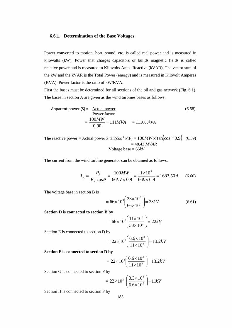
183
6.6.1. Determination of the Base Voltages
Power converted to motion, heat, sound, etc. is called real power and is measured in
kilowatts (kW). Power that charges capacitors or builds magnetic fields is called
reactive power and is measured in Kilovolts Amps Reactive (kVAR). The vector sum of
the kW and the kVAR is the Total Power (energy) and is measured in Kilovolt Amperes
(KVA). Power factor is the ratio of kW/KVA.
First the bases must be determined for all sections of the oil and gas network (Fig. 6.1).
The bases in section A are given as the wind turbines bases as follows:
Apparent power (S) = Actual power (6.58)
Power factor
= MVAMW
11190.0
100 = 111000kVA
The reactive power = Actual power x tan(cos-1
P.F) = 9.0costan100 1MW (6.59)
= 48.43 MVAR
Voltage base = 66kV
The current from the wind turbine generator can be obtained as follows:
9.066
100
cos
kV
MW
E
PI
A
AA
A
k50.1683
9.066
101 5
(6.60)
The voltage base in section B is
kV331066
10331066
3
33
(6.61)
Section D is connected to section B by
= kV221033
10111066
3
33
Section E is connected to section D by
= kV2.131011
106.61022
3
33
Section F is connected to section D by
= kV2.131011
106.61022
3
33
Section G is connected to section F by
= kV11106.6
103.31022
3
33
Section H is connected to section F by

184
= kV11106.6
103.31022
3
33
Table 6.3. The base impedances and currents
Bus
kV
Base ohms = MVA
kV2
Base amperes = kV
kVA
3
Ampere
A 66 39.2400 971
B 33 9.8100 1942
C 33 9.8100 5826
D 11 1.0900 5826
E 6.6 0.3924 9710
F 6.6 0.3924 9710
G 3.3 0.0981 19420
H 3.3 0.0981 19420
Convert transformer impedances to per unit using
Per unit Z2 = per unit Z1
1
2
2
2
2
1
kVAbase
kVAbase
kVbase
kVbase h (6.62)
Subscripts 1 refer the old base condition
Subscripts 2 refer the new base condition
Table 6.4. Convert transformer impedances to per unit
Xh%
p.f
kV1
kV2
MVA
kVA1
kVA2
T1 1+j10 0.87 33 33 100 100000 111000
T2 0.8+j7 0.85 11 22 80 80000 111000
T3 0.7+j6 0.86 6.6 13.2 30 30000 111000
T4 0.7+j6 0.85 6.6 13.2 10 10000 111000
T5 1+j9 0.90 3.3 11 20 20000 111000
T6 0.6+j5.75 0.85 3.3 11 10 10000 111000
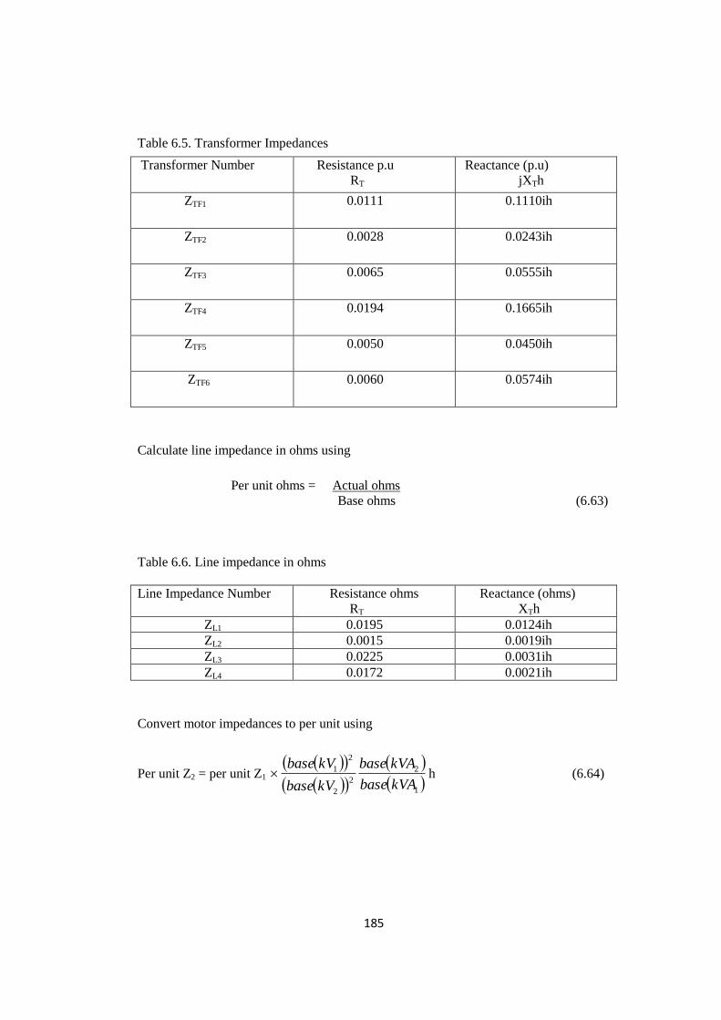
185
Table 6.5. Transformer Impedances
Transformer Number Resistance p.u
RT
Reactance (p.u)
jXTh
ZTF1 0.0111 0.1110ih
ZTF2 0.0028 0.0243ih
ZTF3 0.0065 0.0555ih
ZTF4 0.0194 0.1665ih
ZTF5 0.0050 0.0450ih
ZTF6 0.0060 0.0574ih
Calculate line impedance in ohms using
Per unit ohms = Actual ohms
Base ohms (6.63)
Table 6.6. Line impedance in ohms
Line Impedance Number Resistance ohms
RT
Reactance (ohms)
XTh ZL1 0.0195 0.0124ih
ZL2 0.0015 0.0019ih
ZL3 0.0225 0.0031ih
ZL4 0.0172 0.0021ih
Convert motor impedances to per unit using
Per unit Z2 = per unit Z1
1
2
2
2
2
1
kVAbase
kVAbase
kVbase
kVbase h (6.64)

186
Table 6.7. Convert motor impedances to per unit
Motor
Num
ber
Xh%
p.f
kV1
kV2
MVA
kVA1
kVA2
M1 30 0.60 10.5 66 60 60000 111000
M2 26.6 0.85 10 66 25 25000 111000
M3 22.9 0.65 9.2 66 50 50000 111000
M4 20.5 0.86 10 66 30 30000 111000
M5 18.7 0.58 6.5 66 40 40000 111000
M6 15.2 0.85 6 66 35 35000 111000
M7 13.5 0.86 5.2 66 20 20000 111000
Table 6.8. Motor impedances
Motor Number Resistance p.u
RM
Reactance (p.u)
jXhM
ZM1 0 0.0140ih
ZM2 0 0.0271ih
ZM3 0 0.0099ih
ZM4 0 0.0174ih
ZM5 0 0.0050ih
ZM6 0 0.0040ih
ZM7 0 0.0047ih
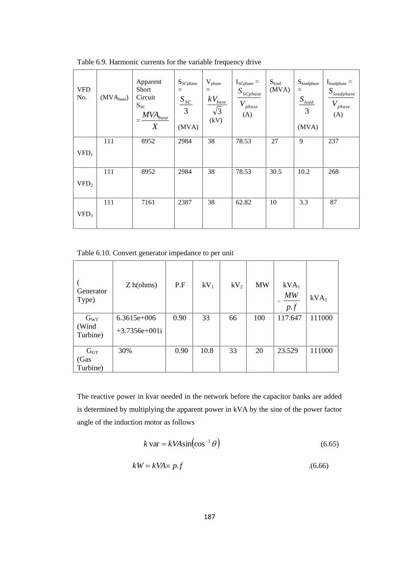
187
Table 6.9. Harmonic currents for the variable frequency drive
VFD
No.
(MVAbase)
Apparent
Short
Circuit
SSC
=X
MVAbase
SSCphase
=
3
SCS
(MVA)
Vphase
=
3
basekV
(kV)
ISCphase =
phase
SCphase
V
S
(A)
Sload
(MVA)
Sloadphase
=
3
loadS
(MVA)
Iloadphase =
phase
loadphase
V
S
(A)
VFD1
111 8952 2984 38 78.53 27 9 237
VFD2
111 8952 2984 38 78.53 30.5 10.2 268
VFD3
111 7161 2387 38 62.82 10 3.3 87
Table 6.10. Convert generator impedance to per unit
(
Generator
Type)
Z h(ohms)
P.F
kV1
kV2
MW
kVA1
=
fp
MW
.
kVA2
GWT
(Wind
Turbine)
6.3615e+006
+3.7356e+001i
0.90 33 66 100 117.647 111000
GGT
(Gas
Turbine)
30% 0.90 10.8 33 20 23.529 111000
The reactive power in kvar needed in the network before the capacitor banks are added
is determined by multiplying the apparent power in kVA by the sine of the power factor
angle of the induction motor as follows
1cossinvar kVAk (6.65)
fpkVAkW . .(6.66)

188
Table 6.11. Generator impedance
Gas Turbine
(Emergency
Generator)Number
Resistance p.u
R
Reactance (p.u)
jXh
ZWT 1.5005e+009 8.8114e+003ih
ZGT 0 1.5159e+002ih
For Capacitor bank1and determined from motor1 (M1) data
Apparent power (S) = 60000 kVA
p.f = 0.60
0.60 to be improved to 0.85 by the capacitor bank1
1 cos-1
0.60 = 53.13o 2 cos
-10.85 = 31.79
o
A = 60000 kVA E = B = 36000 kW
B = 60000 * cos 53.13 = 36000 kW D = 36000 / cos 31.79 = 42354
kVA
C = sqrt(A2 – B
2) = 48000 kvar F = sqrt(D
2 – E
2) = 22313 kvar
The rating of the capacitor = 48000 – 22313 = 25687 kvar
The capacitor bank impedances (Xcap) can be obtained as represented in Table 6.6
It should be reiterated here that Eqn.(6.17) remains constant before and after the
capacitor banks are added.
The rating of the capacitor banks depends solely on the apparent power and power
factor of the induction motors that is required to improve its power factor to 0.85
lagging.
Before adding capacitor
bank 1 (C1)
After adding capacitor
bank 1 (C1)

189
Table 6.12: Capacitor bank impedances
Capacitor bank
Number
(kV)2
kvar
Xcap =
var
2
k
kVh
C1 66 25687 0.1700ih
C2 66 17855 0.2440ih
C3 66 18205 0.2393ih
CACTUAL 66 144619 0.0301h
The nodal admittance matrix of Fig. 6.1 is obtain as follows
hZhZ
hZhBhC
hZhZ
hZhZ
hZhZhChC
hBhZhZhZhZ
hZhZhZhZhZhZhZ
Y
MM
hTFSVCMTF
TFTL
TFTL
SVCMMMTF
TLTFLMTLTFIG
h
76
62
3
5
33
33
21
13324
332111
11
111
1
1
11111
11111
5
(6.67)
The nodal impedance matrix at each harmonic order is obtained as follows
The nodal admittance matrix is a useful tool for the determination of the system
harmonic voltage, the transfer impedance and the deriving point impedance at each
frequency of the converter harmonic order. The non-linear load at PCC2 is represented
by a current injection source if and the solution of the system is obtained by
superposition of source effect.
1 hh YZ (6.68)
Once hZ , is obtained at each characteristic harmonic, the voltage magnitude can be
calculated at each harmonic as follows:

190
hhh IZV (6.69)
where
hI = the source current at each characteristic harmonic
Further analysis can be performed using the individual harmonic voltages and currents.
It may be important to investigate quantities such as the total harmonic distortion
(THD), fault current, harmonic resonance, voltage dip and etc
6.6.2. Further Simulation Results
Motors draw reactive current to support their magnetic fields in order to cause rotation.
Excessive reactive current is undesirable because it creates additional resistance losses
and can require the use of larger transformers and wires. In addition, utilities often
penalize owners for low power factor. Decreasing reactive current will increase power
factor.
Typical AC motors may have a full load power factor ranging from 0.84 to 0.88. As the
motor load is reduced, the power factor becomes lower. Utilities may require site power
factor values ranging from 0.85 to 0.95 and impose penalties to enforce this
requirement. Power factor correction capacitors can be added to reduce the reactive
current measured upstream of the capacitors and increase the measured power factor. To
prevent damage to the motor, power factor correction capacitors should not exceed the
motor manufacturer’s recommendations. In most cases, this results in maximum
corrected values of 0.90 to 0.95.
A lot of motor loads are used in the oil and gas as seen in Fig. 6.1, many compensation
capacitors bank have been installed to improve the power factor. Unfortunately, these
capacitors have introduced serious parallel resonance problems and cause detrimental
effect to the electrical facilities in the platform as represented in Fig. 6.32a.
Harmonic current components that are close to the parallel resonant frequency are
amplified.
Higher order harmonic currents at the PCC1 and PCC2 are reduced because the
capacitors are low impedance at these frequencies. The Fig. 6.32a below shows the
effect of adding capacitors on the 11kV and 6.6kV buses for power factor correction.
This figure shows that by adding some typical sizes of power factor correction
capacitors will result in the magnification of the 5th and 25
th harmonic components,
which in turns makes it even more difficult to meet the IEEE 519-1992 harmonic
current standards.

191
More also, large harmonic voltages as observed in Fig. 6.32b and 6.32c are introduced
at these harmonic resonant even though the harmonic current flow is small. To avert the
harmonic resonance problem, it is necessary to install compensator equipment such as
SVC or filter on the distribution network platform.
0 5 10 15 20 25 30 35 40 45 500
1
2
3
4
5
Harmonic Order
|Z|p
.u.
ohm
s
Harmonic Impedance
0 5 10 15 20 25 30 35 40 45 500
0.05
0.1
0.15
0.2
Harmonic Order
|V|p
.u.
kV
Harmonic Voltage
(b)
(a)

192
0 5 10 15 20 25 30 35 40 45 500
0.05
0.1
0.15
0.2
Harmonic Order
|V|p
.u.
kV
Harmonic Voltage
Figure 6.32. (a) Harmonic resonance impedance with capacitor bank (b) Harmonic
voltage spectrum of PCC one (c) Harmonic voltage spectrum of PCC two
6.6.3. Impact of Advance Static Var Controller (ASVC)
The fixed capacitor banks are supported with ASVC represented in Fig. 6.33 of suitable
rating to compensate fully for the reactive power requirement. In order to investigate the
performance of ASVC on the oil platform distribution network, some choices have been
made regarding the system studies. The rating of the ASVC is 300 Mvar and its firing
angle that would require to achieve this Mvar is obtain via carrying out sufficient
Newton-Raphson iterations that will satisfy a firing angle mismatch of less than
1x10⁻³
. Where TCR = 90o at the initial starting condition.
Figure 6.33. Static Var compensator
QTCR = 0.6 p.u
jXC = -j0.10 p.u
jXL = 0.05 p.u
TCR
Vl
Ih
(c)

193
The capacitor’s susceptance is:
C
CjX
jB
1
(6.70)
For the Thyristor-controlled reactor (TCR), we have,
L
TCRjX
jB2sin2
(6.71)
The combined susceptance is:
TCRCSVC jBjBjB (6.72)
In more detained form:
LC
CL
SVCXX
jXjXjB
sin2 (6.73)
The SVC equivalent impedance at fundamental frequency, ZSVC is obtained as follow
SVC
SVCjB
jZ1
(6.74)
The SVC current is:
lSVCSVC VZjI (6.75)
and complex power is:
SVClSVC IVS
= 22sin2
l
LC
CL VXX
XXj
(6.76)
Since the SVC under consideration contains no resistance then no active power exists in
the circuit. Hence,
0SVCP (6.77)
LC
LC
SVCXX
XXQ
2sin2 2
lV (6.78)
or
0222sin2
l
SVCL
C
L
V
QX
X
X (6.79)

194
Using the Newton-Raphson iterative method to solve for the firing angle, using the
following Equations
2222sin
l
SVCL
C
L
V
QX
X
Xf (6.80)
and
22cos2
ff (6.81)
f
f1
0
(6.82)
o18000`1 (6.83)
In order to enable both absorption and the injection of reactive power at the point of
common coupling (PCCs), the SVC will have to changes from the inductive region to
the capacitive region as the firing angle increases. In this test result the SVC generated
maximum reactive power from capacitive region into the network as shown in Fig.
6.34a at 90o
< 180o. Partial impedance appears at the bus where harmonic
resonance occurs that is, partial 15th harmonics, so no large harmonic voltages including
15th harmonics are observed in Fig. 6.34b and 6.34c.
As illustrated in Fig. 6.34b and 6.34c the variation of reactive power with firing angle is
non-linear. Also, these figures shows that the SVC generates 5th ,25
th and 35
th harmonics
and the three-phase SVC are delta connected to prevent the triplen harmonics from
spreading to the oil platform.
0 5 10 15 20 25 30 35 40 45 500
0.5
1
1.5
2
2.5
3
Harmonic Order
|Z|p
.u.
ohm
s
Harmonic Impedance
(a)
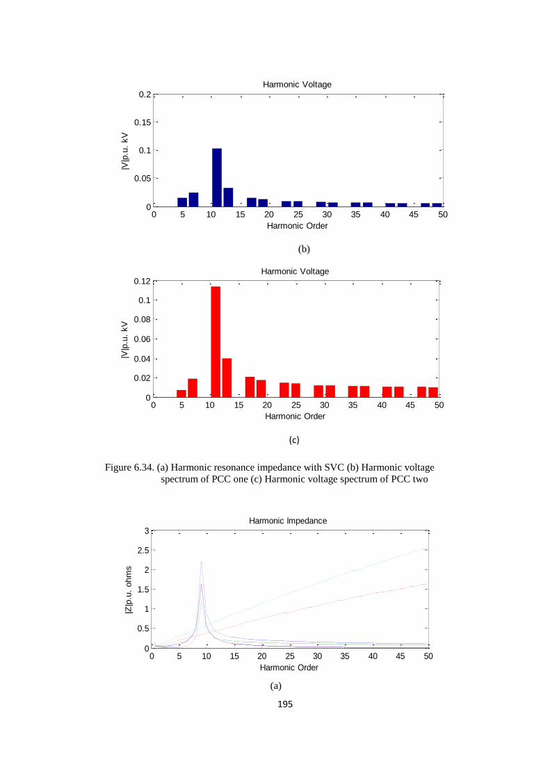
195
0 5 10 15 20 25 30 35 40 45 500
0.05
0.1
0.15
0.2
Harmonic Order
|V|p
.u.
kV
Harmonic Voltage
(b)
0 5 10 15 20 25 30 35 40 45 500
0.02
0.04
0.06
0.08
0.1
0.12
Harmonic Order
|V|p
.u.
kV
Harmonic Voltage
(c)
Figure 6.34. (a) Harmonic resonance impedance with SVC (b) Harmonic voltage
spectrum of PCC one (c) Harmonic voltage spectrum of PCC two
0 5 10 15 20 25 30 35 40 45 500
0.5
1
1.5
2
2.5
3
Harmonic Order
|Z|p
.u.
ohm
s
Harmonic Impedance
(a)

196
0 5 10 15 20 25 30 35 40 45 500
0.02
0.04
0.06
0.08
Harmonic Order
|V|p
.u.
kV
Harmonic Voltage
(b)
0 5 10 15 20 25 30 35 40 45 500
0.02
0.04
0.06
0.08
Harmonic Order
|V|p
.u.
kV
Harmonic Voltage
(c)
Figure 6.35. (a) Harmonic resonance impedance with SVC and capacitor bank(b)
Harmonic voltage spectrum of PCC one (c) Harmonic voltage spectrum of
PCC two
0 5 10 15 20 25 30 35 40 45 500
1
2
3
Harmonic Order
|Z|p
.u.
ohm
s
Harmonic Impedance
(a)

197
0 5 10 15 20 25 30 35 40 45 500
0.01
0.02
0.03
0.04
Harmonic Order
|V|p
.u.
kV
Harmonic Voltage
(b)
0 5 10 15 20 25 30 35 40 45 500
0.005
0.01
0.015
0.02
0.025
Harmonic Order
|V|p
.u.
kV
Harmonic Voltage
(c)
Figure 6.36. (a) Harmonic resonance impedance with motor starting (b) Harmonic
voltage spectrum of PCC one (c) Harmonic voltage spectrum of PCC two
The combination of SVC and capacitor banks in the platforms resulted in reducing the
magnitude of the harmonic resonanace impedance as shown in Fig. 6.35a, as observed
there is no indication of odd harmonics comparable to Fig. 6.32 and 6.34. The Fig.
6.35b and Fig. 6.35c represent the harmonic voltage spectrum of PCC 1 and PCC 2
with very low magnitude of 5th , 25
th and 35
th harmonics.
The lower harmonic resonanace impedance magnitude in Fig. 6.36a shows motor
starting with other load interactions. Starting of high capacity induction motors is one
cause of voltage dips. During start-up an induction motor demand voltage five to six
times higher than nominal speed and this takes several seconds, as such voltage dips
occurs.
As observed in Fig. 6.36b and 6.36c shown that harmonics that are multiples of 2 are
not seen because they cancel out. The same is true for 3rd
order harmonics (3rd
, 6th, 9
th
198
etc.). Because the power supply is three-phase, the third order harmonics cancel each
other out in each phase. This leaves only the 5th, 25
th, 35
th etc.
The magnitude of the harmonics produced by SVC and capacitor banks is greatest for
the lower order harmonics (5th) and drops quickly as you move into the higher order
harmonics (35th and greater).
6.6.4. Impact of Tuned Reactor Filter
The little harmonic resonance peak in Fig. 6.36a could be avoided by installing tuned
frequency filter. In order to avoid this harmonic magnification we choose a tuned
frequency less than nine. The frequency characteristic of the tuned filter at 7th
harmonics is shown Fig. 6.41 using the following equations.
capf
base
fkVARh
fkVL
2
2
2
1000
(6.84)
CLf
f
resonance2
1 (6.85)
where
f – fundamental frequency (50Hz)
hf – harmonic level frequency (e.g for 7th harmonic level frequency =
750 = 350Hz
As it can be seen from the Fig. 6.37a harmonic resonance in the system has been
removed. Moreover, there is some reduction for all the other harmonic components as
shown in Fig. 6.37b and Fig. 6.37c

199
0 5 10 15 20 25 30 35 40 45 500
0.5
1
1.5
2
2.5
3
Harmonic Order
|Z|p
.u.
ohm
s
Harmonic Impedance
0 5 10 15 20 25 30 35 40 45 500
1
2
3
4x 10
-56
Harmonic Order
|V|p
.u.
kV
Harmonic Voltage
0 5 10 15 20 25 30 35 40 45 500
0.5
1
1.5
2x 10
-29
Harmonic Order
|V|p
.u.
kV
Harmonic Voltage
Figure 6.37. (a) Harmonic resonance with tune filter (b) Harmonic voltage spectrum of
PCC one (c) Harmonic voltage spectrum of PCC two
The harmonic current of the SVC and capacitor bank can be determine using the
following relations,
(a)
(b)
(c)

200
h
SVC
TOTAL
SVC IZ
ZI (6.86)
hTOTAL
C
TOTAL
C IZZ
ZI
(6.87)
10 15 20 25 30 35 40 45
-10
-5
0
5
Harmonic Order
SV
C (
1&
2)a
nd C
apacitor
Curr
ent
Isvc1
Isvc
IC
Vh
Figure 6.38. SVC current and capacitor current as afunction of system impedance
Figure 6.38shows the behaviour of the SVC and capacitor current and harmonic voltage.
As observed the SVC current is absolutely reactive region, while the capacitor current is
purely active region and harmonic voltage is acting from the apparent region. These
indicate that the majority of the reactive power is supplied by the SVC. The harmonic
currents appears not to contain lower harmonics such as 3rd
, 5th, 7
th and 9
th (h = 2k+1,
with k = 1,2,3...) harmonics.
6.7. Conclusions
It is possible to suggest that renewable energy in the form of wind energy could become
economically viable within oil and gas production field in future. The large actual
power MW produced by wind energy may lower harmonic distortion on the PCC
voltage. The reduction of CO2 and the fact that wind source is free presents the real
possibility that wind energy might become the energy source of choice for the oil and
gas industry.

201
The harmonic currents induce harmonic voltages at the PCC. The impedance harmonic
depends on the harmonic current injection to the PCC and the resulting harmonic
voltage is computed. The harmonic distortion on the PCC voltage caused by harmonic
current drawn by the nonlinear loads on the oil platform, this causes the harmonic
current to flow through the pure linear resistive load.
After respective computational implementation of the model, there followed a set of
studies for the evaluation of a simplified power factor capacitor bank compensation,
comparable to SVC. Although, the capacitor compensation improved the power factor
correction of the induction motor, it also introduced harmonic resonance problem in the
system. This problem could be averted using appropriate SVC as seen. The reduction of
the harmonic components and harmonic resonance is mainly, by the replacement of
capacitor bank or use of both.
In investigating the performance of ASVC at distribution systems network some
choices have been made regarding system studies, the ASVC, and a tool for harmonic
control. The radial model has been chosen as the study system. This choice has been
motivated by the fact that the model has been established to provide a common
reference system to researchers conducting comparative performance studies, either of
component interactions or of harmonic control concepts. Some modifications of the
system have been carried out to create a very weak ac system at the inverter site.
6.8. References
[1] P.E.R.Walling, and D.Mueller,“Harmonics and Resonance Issues in Wind Power”.
IEEE PES General Meeting, July 26th, 2011.
[2] M. Hacil, A. Khezzar, A.L. Nemmour and L. Louze,” Harmonic current
cancellation and control of a grid-connected synchronous generator entrained by
a wind turbine”. Revue des Energies Renouvelables Vol. 12 N°3 (2009) 405 – 418
[3] F. Blaabjerg and Z. Chen, “Power Electronics for Modern Wind Turbines”, 1st ed.
Morgan & Claypool, 2006.
[4] Ł.H.Kocewiak, J.Hjerrild, and C. L. Bak, “Harmonic Analysis of Offshore Wind
Farms with Full Converter Wind Turbines”.

202
[5] C.H.Chien, R.W.G. Bucknall,“Theoretical Aspects of the Harmonic Performance
of Subsea AC Transmission Systems for Offshore Power Generation Schemes”,
in Proc. Generation Transmission and Distribution, 2006, p. 599-609.
[6] J.Arrillage, B.C.Smith, N.R.Watson, and A.R.Wood, “Power System Harmonic
Analysis”.ISBN 0 471 97548 6. 1997
[7] O.Anaya-Lara, N.Jenkins, J.Ekanayake, P.Cartwright, and M.Hughes, “Wind
Energy Generation Modelling and Control”. ISBN 978-0-470-71433-1 (H/B).
2009.
[8] W.Shepherd, and L.Zhang, “Electricity Generation using Wind Power” ISBN 13
978-981-4304-13-9. 2011.
[9] L. Asiminoaei, F. Blaabjerg and S. Hansen, “Evaluation of Harmonic Detection
Methods for Active Power Filter Applications” Applied Power Elec. Conf. and
Expo. (APEC), Vol. 1, pp.635-641, 2005.
[10] T.B. Soeiro, M.Schweizer, J.Linner, P.Ranstad and J.W. Kolarl, “Comparison of
2- and 3-level Active Filters with Enhanced Bridge-Leg Loss Distribution”.
[11] E.Acha, J.Arrillaga,A. Medina. and A.Semlyen, “General frame of reference for
analysis of distortion in system with multiple transformer nonlinearities”,
Proc.IEE Pt. C, Vol. 136, No.5, September, pp. 271-278. (1989),
[12] E.Acha, and J.J.Rico ,“Harmonic domain modelling of non-linear power plant
components”, ICHPS Conference, Bologna, Italy. (1994).
[13] S.Ganesan, “Selection of Current Transformers and Wire Sizing in Substations”
ABB Inc.
[14] R.D.Henderson, and P.J.Rose,”Harmonics: The effects on Power Quality and
Transformers”, IEEE Trans Industry Appllication 1994, Vol 30(3), pp 528-532.
[15] S.I.Shahl, “Electrical Machines II”.
[16] A.L.Sheldrake,” Handbook of Electrical Engineering for Practitioners in the Oil,
Gas and Petrochemical Industry” ISBN 0-471-49631-6. 2003
[17] IEEE Recommended Practice for “Power Systems Analysis”, IEEE Std. 399-
1990.
[18] Y. Goo, J. N. Jiang, and C.Y. Tang, “Nonlinear Control of Wind Power
Generation Systems,” 2009 IEEE Xplore.
[19] M. Liserre, R. Cardenas, M. Molinas, and J. Rodriguez, “Overview of multi-MW
wind turbines and wind parks,” IEEE Trans. Ind. Electron., vol. 58, no. 4, pp.
1081–1095, Apr. 2011.
[20] F. Van Hulle and N. Fichaux, “Powering Europe: Wind energy and the electricity
grid,” Eur. Wind Energy Assoc., Brussels, Belgium, Nov. 2010.
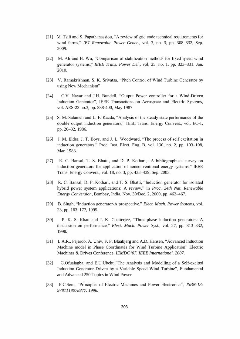
203
[21] M. Tsili and S. Papathanassiou, “A review of grid code technical requirements for
wind farms,” IET Renewable Power Gener., vol. 3, no. 3, pp. 308–332, Sep.
2009.
[22] M. Ali and B. Wu, “Comparison of stabilization methods for fixed speed wind
generator systems,” IEEE Trans. Power Del., vol. 25, no. 1, pp. 323–331, Jan.
2010.
[23] V. Ramakrishnan, S. K. Srivatsa, “Pitch Control of Wind Turbine Generator by
using New Mechanism”
[24] C.V. Nayar and J.H. Bundell, “Output Power controller for a Wind-Driven
Induction Generator”, IEEE Transactions on Aerospace and Electric Systems,
vol. AES-23 no.3, pp. 388-400, May 1987
[25] S. M. Salameh and L. F. Kazda, “Analysis of the steady state performance of the
double output induction generators,” IEEE Trans. Energy Convers., vol. EC-1,
pp. 26–32, 1986.
[26] J. M. Elder, J. T. Boys, and J. L. Woodward, “The process of self excitation in
induction generators,” Proc. Inst. Elect. Eng. B, vol. 130, no. 2, pp. 103–108,
Mar. 1983.
[27] R. C. Bansal, T. S. Bhatti, and D. P. Kothari, “A bibliographical survey on
induction generators for application of nonconventional energy systems,” IEEE
Trans. Energy Convers., vol. 18, no. 3, pp. 433–439, Sep. 2003.
[28] R. C. Bansal, D. P. Kothari, and T. S. Bhatti, “Induction generator for isolated
hybrid power system applications: A review,” in Proc. 24th Nat. Renewable
Energy Conversion, Bombay, India, Nov. 30/Dec. 2, 2000, pp. 462–467.
[29] B. Singh, “Induction generator-A prospective,” Elect. Mach. Power Systems, vol.
23, pp. 163–177, 1995.
[30] P. K. S. Khan and J. K. Chatterjee, “Three-phase induction generators: A
discussion on performance,” Elect. Mach. Power Syst., vol. 27, pp. 813–832,
1998.
[31] L.A.R.. Fajardo, A. Univ, F. F. Blaabjerg and A.D..Hansen, “Advanced Induction
Machine model in Phase Coordinates for Wind Turbine Application” Electric
Machines & Drives Conference. IEMDC '07. IEEE International. 2007.
[32] G.Ofualagba, and E.U.Ubeku,”The Analysis and Modelling of a Self-excited
Induction Generator Driven by a Variable Speed Wind Turbine”, Fundamental
and Advanced 250 Topics in Wind Power
[33] P.C.Sem, “Principles of Electric Machines and Power Electronics”, ISBN-13:
9781118078877. 1996.

204
[34] J.A.Restrepo, U.B.Simon, P.Bowler, “Analysis of induction machine slot
harmonics in the TF domain”, Devices, Circuits and Systems, 1995, Proceedings
of the 1995 First IEEE International Caracas Conference on Dec 1995.
[35] D.C.Sue,” High Efficiency Double-Fed Induction Generator Applied to Wind
Power Generator Technical Analyses”. Energy and Power Engineering, 2011, 3,
253-261.
[36] IEEE Standard Test Procedure for Polyphase Induction Motors and Generator,
IEEE Std 112-2004, 2004.
[37] W Deprez, A Dexters, J Driesen, “Energy efficiency of small induction machine.
Comparison between motor and generating mode” - ICEM 2006, 2006 -
esat.kuleuven.be
[38] E.Muljadi, J.Sallan, M,Sanz , and C.P. Butterfield,” Investigation of Self-Excited
Induction Generators for Wind Turbine Applications”, February 2000 .
NREL/CP-500-26713.
[39] A. K. Tandon, S. S. Murthy and G. J. Berg, “Steady State Analysis of Capacitor
Self-excited Induction Generators,” IEEE Transactions on Power Application
Systems, Vols. PAS-103, no. 3, pp. 612-618, March 1984.
[40] L. Quazene and G. McPherson, “Analysis of the Isolated Induction Generator,”
IEEE Transactions on Power Apparatus and Systems, Vols. PAS-102, no. 8, pp.
2793-2798, August 1983.
[41] S. S. Murthy, O. P. Malik and A. K. Tandon, “Analysis of Self-excited Induction
Generators,” IEE Proceedings C on Generation, Transmission and Distribution,
vol. 129, no. 6, pp. 260-265, November 1982.
[42] S. Rajakaruna and R. Bonert, “A Technique for the Steady-state Analysis of a
Self-excited Induction Generator with Variable Speed,” IEEE Transactions on
Energy Conversion, vol. 8, no. 4, pp. 757-761, December 1993.
[43] S. S. Murthy, G. Bhuvaneswari, S. Gao and R. K. Ahuja, “Self Excited Induction
Generator for Renewable Energy Applications to Supply Single-phase Loads in
Remote Locations,” in IEEE International Conference on Sustainable Energy
Technologies, Kandy, December 2010.
[44] L. Wang and C. H. Lee, “A Noval Analysis of the Performance of an Isolated
Self-excited Induction Generator,” IEEE Transactions on Energy Conversion,
vol. 12, no. 2, pp. 109-115, June 1997.
[45] I. Boldea and S. A. Nasar, The Induction Machine Handbook, Florida: CRC
Press, 2002.
[46] A.M.Sharaf,and S.K.Murugan, “Dynamic power filter & capacitor compensator
for isolated self-excited induction generator driven by a wind turbine”.

205
Harmonics and Quality of Power, 2004. 11th International Conference on Sept.
2004.
[47] E. Muljadi, C.P. Butterfield, H. Romanowitz, and R. Yinger “Self Excitation and
Harmonics in Wind Power Generation”. November 2004 • NREL/CP-500-33138.
[48] M. Bradt, B. Badrzadeh, E. Camm, D. Mueller, J. Schoene, T. Siebert, T. Smith,
M. Starke, and R. Walling, “Harmonics and Resonance Issues in Wind Power
Plants”. IEEE PES Wind Plant Collector System Design.
[49] A.V.Jacn, E.Acha, and A.Gomez, “Voltage Source Converter Modelling for
Power System State Estimation: STATCOM and VSC-HVDC”. IEEE
Transaction on Power Systems Vol. 23. No. 4 Nov. 2008.
[50] P.W.Lehn, and K.L.Lian, “Frequency Coupling Matrix of a Voltage Source
Converter Derived from Piecewise Linear Differential Equations”. IEEE
Transaction on Power Delivery. Vol.22. July 2007.
[51] P. W. Lehn,” Direct Harmonic Analysis of the Voltage Source Converter”. IEEE
Transactions on Power Delivery, Vol. 18, No. 3, July 2003

206
CHAPTER 7
7. Harmonic Modelling of Multi-Terminal HVDC-VSC Oil and Gas
Platforms
7.1. Introduction
The flexibility of VSC (AC-DC and DC-AC converters) technology has shown a strong
competitive advantage in interconnecting different oil and gas platforms, functioning as
the firewall against outages expanding and propagating [1-5]. For the AC grid, which
has already experienced an outage or blackout, it can be started up by using a VSC-
HVDC station [6]. It can provide effective voltage and frequency stabilization during
the restoring process when the network experiences dramatic changes from zero short-
circuit power to normal short-circuit power. This will make the restoration less
complicated and more reliable [7].
VSC has two degrees of freedom, namely amplitude modulation index (ma) and the
phase displacement (φ) [8]. These flexibilities together with its fixed voltage polarity for
both rectifier and inverter modes of operation make VSC-HVDC the core component in
developing multi-terminal oil and gas platforms as shown in Fig. 7.1.
The main function of the VSC-HVDC is to transmit constant DC power from the
rectifiers to the inverters [9]. A VSC-HVDC link is also capable of transferring the
active power from the grid and, at the same time, decreasing the disturbances from the
utility grid [10]. When a VSC-HVDC supplies the oil and gas platform network, the
inverter of the VSC-HVDC can use the AC voltage and frequency controllers to keep
the load side AC voltage and frequency constant. In this way power-quality
disturbances like voltage dips do not reach the oil and gas platform installations
[11][12].
The aim of this chapter is to develop a flexible and robust multi-terminal VSC-HVDC
model to implement harmonic power flow computational method. This is necessary for
harmonic current injection and to carry out harmonic propagation studies in oil and gas

207
platform power systems. The harmonic power flow solution is aimed to derive
fundamental frequency information for the voltage magnitudes and angles at all nodes
of the network.
When using a conventional power flow, the assumption is made that all elements of the
power system will not produce harmonics of fundamental frequency voltages and
currents. These may include the transmission network, and any devices attached to
generator or load buses. Conventional power flows do not allow the inclusion of
harmonic devices, which are power system elements which will distort fundamental
frequency voltages and currents [13].
A harmonic power flow is a tool which can predict the level and propagation of
harmonics created by one or more harmonic device in the power system, the effects
thereof, and the exploration of corrective measures using filtering techniques [14].
The harmonic power flows discussed in this chapter, only consider power systems
operating in a completely balanced three-phase mode. Each phase of the three-phase
power system contains identical fundamental and harmonic voltages and currents. One
property of a completely balanced power system is that even harmonic currents and
voltages do not exist. With completely balanced conditions assumed, a single line
admittance (impedance) diagram of the power system may be used for each harmonic
considered. In addition, the admittances (impedances) of each single line diagram must
be scaled according to the harmonic frequency [15-16].
If unbalanced conditions exist, fundamental and harmonic currents each contain
positive-, negative-, and zero-sequence components. The method of symmetrical
components must then be used to simplify analysis, but will not be considered in this
chapter. For this reason, all buses which contain harmonic producing devices will be
referred to as harmonic buses.
All the passive elements are considered to perform linearly with frequency and the
linear elements whose harmonic impedance is derived similarly to passive element. All
non-linear loads are represented by either a harmonic current injection source or by a
harmonic voltage source. Harmonic current injection sources are used to represent the
harmonic contributions of rectifiers, inverters, static VAR compensators (SVCs).

208
Harmonic voltage sources are arc furnaces, and VSC, pulse-width modulation (PWM)
converters.
Figure 7.1. Multi-terminal network with modular multi-level converter used to obtain
the driving point impedance and harmonic propagation
XT2
XT1
66kV
TX3
TX4
TX2 150km
66kV
66kV
66kV
TX1
100MW
100MW
0.0600+j0.1800
Bus 5
Bus 4 Bus 3
Bus 2
Bus 1
Xv
HVDC-VSC
MMC
MMC
MMC MMC
MMC
Oil and Gas Platform 1
Oil Refinery
Platform 2
LNG
Platform 3
Modular Multi-
level
Converter (MMC)
HVDC-VSC
100km
actor
V
Re
0.0452+j0.1652
0.0472+j0.1983
0.0132+j0.0379
0.0570+j0.1737
0.0581+j0.1763

209
Transmission elements and linear loads are represented by impedances, at each
harmonic h, with which the admittance matrix Yh of the system is developed. The
relevant harmonic current and voltage sources Ih and Vh are injected into the partially
inverted nodal admittance matrix and the remaining nodal harmonic voltages and
currents are derived using the Newton-Raphson method.
7.2. Harmonic Power Flow
It was mentioned in chapter one that VSC is referred to as self-commutated converters
and is termed harmonic voltage source just as the name implies. With this capability
VSC connected at all the nodes as shown in Fig. 7.1 provide voltage required at the
nodes. Being a nonlinear component it is a source of harmonics in power networks [17].
This characteristic is of great importance in the harmonic power flow (HPF), to
accurately model the nonlinear relationship between the current and voltage waveforms
at each bus containing a harmonic device. For this reason, it is convenient to express
distorted voltages and currents as Fourier Series (FS). In the case of HPF, the FS of the
current entering a bus containing a harmonic device is expressed as a function of the FS
of the voltage at this bus, and of any parameters which describe this distorted current
waveform.
The harmonic voltage injection into the nodal signal can be expressed as follows
htMtMtv hhan 000 coscos)( (7.1)
htMtMtv hhbn
000 cos
3
2cos)( (7.2)
htMtMtv hhcn
000 cos
3
2cos)( (7.3)
7.2.1. Switching Function Mode of the Rectifier Process
In Figure 7.1 input lines are connected to the output lines by bidirectional switching
function (SF) and the single frequency (PWM) modulating signal form the matrix

210
converter. Each switch is operated by a diagonal switching function, diag(SFrc (t)),
where r denotes the row vectors and c the column vectors as represented in (7.4).
The switching function matrix SFrc connecting the three-phase output voltages in Fig.
7.1 is given as
ca
bc
ab
rc
SF
SF
SF
SF
00
00
00
(7.4)
The choice of the switching matrix determines the frequency, the amplitude and the
phase of the output. The switches must be operated in such a way that the voltage and
current Kirchoff’s laws are not violated [18]. That is
At all times, each of the output lines are connected to input lines otherwise fault
will be generated by the inductive load which may damage the IGBTs switches
No two input lines must be connected at the same time to the same outline
otherwise a short circuit will emerge.
The output current (Idc), is forced to flow through the load by the output voltage (Vdc).
The mathematical model for matrix converter representing its basic operation is simple.
From Figure 5.1 (Chapter 5) the harmonics of the six switching functions SFab,bc,ca
voltages are
3
10 vS (7.5)
2
23sin
23sin
2
1 prjn
vp ennn
SF (7.6)
where
r is the shift angle of the AC voltage supply with respect in the reference
tVtv aa 0sin
p is the sequence phase angle required to fire the IGBTs per SM. i.e.
Table 7.2 The sequence phase angle
Angle
p
0 3
3
2
3
4
3
5
IGBT 1 2 3 4 5 6
is the firing angle

211
The output voltage of the converter sub-module (SM) leg A, B, C are given by
hSFma
V vaoutA2
(7.7)
hSFma
V vboutB2
(7.8)
hSFma
V vcoutC2
(7.9)
where ma is the modulation index and SFv…is switching function voltages
The phase voltage
nphoutAa VVV (7.10)
nphoutBb VVV (7.11)
nphoutCc VVV (7.12)
It is now understood that the operating principle of an ideal converter without
commutation process can be linked as the process of modulating the ac side voltage
with a switching function to obtain the DC voltage as
aabdc VSFV ; abcdc VSFV ; acadc VSFV (7.13)
7.3. Potential Application of the Admittance (Y) Matrix of the Five Buses
The effect of the DC voltages is evaluated by using impedances connected between
buses in the harmonic network [19]. The value of these impedances depends on the
behaviour of the converter. In the studies performed, the impedance is calculated from
the injection power and the applied bus voltage at the fundamental frequency. In the
presence of harmonics, the resistance remains constant and the reactance is assumed to
vary in direct proportion to the harmonic number. If there is a large compensation or
filter capacitor connected to the bus, it is necessary to separate it from the load and
consider it as an independent branch [20-21]. The admittance at a harmonic frequency is
in direct proportion to the harmonic number.
Transmission lines are distributed parameter devices. In power system analysis, these
lines are usually treated as lumped parameters devices, employing either or T
equivalent circuit. It is important to consider the wave solution only for a long line. In

212
the harmonic domain, the skin effect and wave solution are important and cannot be
ignored as investigated in chapter four. The equation for evaluating the admittance
matrix of the five buses is given by
5
4
2
1
5,5
5,4
4,5
4,4
2,5
2,4
1,5
1,4
5,24,22,21,2
5,14,12,11,1
5
4
2
1
dc
dc
dc
dc
dc
dc
dc
dc
V
V
V
V
Y
Y
Y
Y
Y
Y
Y
Y
YYYY
YYYY
I
I
I
I
(7.14)
The DC current Idc is given by
Idc = Y-1
Vdc (7.15)
where, Y is the admittance matrix of the five bus multi-terminal system
Similarly, the ac current (Iin) can be determined by modulating the DC current with the
current switching function (SF) given as
dcaba ISFI ; dcbcb ISFI ; dccac ISFI (7.16)
The six switching functions for the current are
3
10 iS (7.17)
2
2 23cos
23cos
1 prjn
ip ennn
SF (7.18)
It should be reiterated here that when the converter is operating under unbalanced
source conditions the commutation overlap for each phase will differ. Because the
switching function for each phase will have a different waveform, and as such will
require expression by different equation. Under this condition, the calculation of the
harmonics becomes more complex. In order to avert this complexity, the average
commutation overlap due to the positive sequence voltage may be utilized.

213
7.4. Deriving Unknown Nodal Harmonic Voltages and Currents
The formulation of Newton-Raphson power flow (NR-PF) begins from the basic
network theorems [22]. The voltage source may be transformed to the current source
provided that:
eq
g
sZ
VI (7.19)
where Is is the fundamental frequency current flow at bus i of n-bus system that
corresponds to the one-line diagram of Fig. 7.1.
The apparent complex power S, in volt-amperes is given by
S = P + jQ = VI* VA (7.20)
where I* is the complex conjugate of I.
The bus currents flowing through each bus are given by
yX
xy
x VVjX
I 1
(7.21)
yx
xy
x VVjX
I1
(7.22)
Substituting (7.22) into (7.17) yields
yx
xy
x
x VVjX
VS (7.23)
From the complex conjugate Equ. (7.23) voltage magnitude relate to voltage angle by
11 VV (7.24)
oVV 022 then
*
22 VV (7.25)

214
Substituting the value of Ii =
n
k
kikVY1
into (7.16).
where n is the number of bus and i = 1,2,3,...n).
Therefore,
n
k
kikiii VYVjQP1
** where k = 1,2,3,...n (7.26)
where
Vi is the voltage of the ith bus
Yik is the admittance matrix of the network
Separating (7.26) to real and imaginary parts, yields
n
k
kikii VYVP1
**Re where k = 1,2,3,...n (7.27)
n
k
kikii VYVQ1
**Im where k = 1,2,3,...n (7.28)
where
Pi is the real power
Qi is the reactive power
Substituting ij
ii eVV
, kj
kk eVV
, ikj
ikik eYY
in (7.25), we have
where
iV is the voltage magnitude
i is the voltage angle
ik
is the load angle
ikki j
ik
jn
k
k
j
iii eYeVeVjQP
1
where i = 1,2,3,...n (7.29)
ikkij
ik
n
k
kiii eYVVjQP
1
where i = 1,2,3,...n (7.30)
ikkiik
n
k
kiii YVVjQP 1
where i = 1,2,3,...n (7.31)
ikkiikkiik
n
k
kiii jYVVjQP
sincos1
(7.32)
The real and reactive power of (7.32) are given by
ikkiik
n
k
kii YVVP
cos1
(7.33)

215
ikkiik
n
k
kii YVVQ
sin1
(7.34)
Equations (7.33) and (7.34) are strong tools for Newton-Raphson iterative method.
They constitute a set of nonlinear algebraic equations in terms of the independent
variables, voltage magnitude in p.u., and phase angle in radians. Equation (7.33) gives
the solution for each voltage controlled bus. Equation (7.33) and (7.34) can be expanded
using Taylor’s series neglecting all higher order terms and about the initial estimate will
result in linear equation (7.35) called Jacobian matrix. The components of the Jacobian
matrix are partial derivatives of (7.33) and (7.34) using iV and i .
n
n
Q
Q
P
P
2
2
=
n
nn
n
nn
nn
n
nn
n
nn
nn
V
Q
V
QQQ
JJ
V
Q
V
QQQ
V
P
V
PPP
JJ
V
P
V
PPP
22
2221
2
2
22
2
2
22
1211
2
2
22
2
2
n
n
V
V
2
2
(7.35)
In more compact form, (7.35) can be written as
Q
P =
2221
1211
JJ
JJ
V
(7.36)
The Jacobian matrix (7.36) gives the linearized relationship between voltage magnitude
iV and voltage angle i with respect to changes in real and reactive power.
Also, the admittance matrix (Yik ) in (7.25) its real and reactive parts are separated to
obtain the Conductance (G) and Susceptance (B) matrices.

216
ki jn
k
kikik
j
iii eVjBGeVjQP
1
where i = 1,2,3,...n (7.37)
where ikikik jBGY
ikikik jBGY
kijn
k
kikikiii eVjBGVjQP
1
where i = 1,2,3,...n (7.38)
ki
n
k
kikikiii VjBGVjQP 1
where i = 1,2,3,...n (7.39)
kikiikik
n
k
kiii jjBGVVjQP
sincos1
(7.40)
kiikkiik
kiikkiikn
k
kiiiBGj
BGVVjQP
cossin
sincos
1
(7.41)
From (7.42) the real and reactive power of the network can be computed as
kiikkiik
n
k
kii BGVVP
sincos1
(7.42)
kiikkiik
n
k
kii BGVVQ
cossin1
(7.43)
Equations (7.42) and (7.43) are strong tools for the development of Fast Decoupled
Load Flow (FDLF). This is based on the assumption that, for a transmission line, its
reactance is more than its resistance. That is R
X >> 1, therefore, Gik can be ignored
because Gik << Bik.
The Newton-Raphson method has a quadratic convergence and computing time only
increases linearly with system size.
7.4.1. Newton-Raphson Conventional Power Flow: Test Case 1
The five bus test network of Figure 7.1 has been modelled to perform power flow
studies using the Newton-Raphson iterative method. The base reactive power value is
100 kV and base apparent power is 101 MVA. The transmission lines are nominal -
circuit and its corresponding parameters are given in table 7.1. The modular multi-level

217
dc is based on the multi-level dc system. Therefore, Table 7.2 shows the nodal dc
voltages, voltage angles, PV bus active and reactive powers and PQ bus active and
reactive powers. Bus 5 is chosen to be the slack bus, the line parameter and bus data are
given as in Table A7.1 and Table A7.2.
The appearance of harmonic content in the nodal signal is not rare. It is expected that
different control scenarios in grid-connected converters can include unwanted
distortions or sometimes distortions introduced by a certain control purpose. One good
example is common-mode 3rd
-harmonic injection in order to extend linear operation of
the modulator.
The harmonic injection into the nodal signal can be expressed as depicted in Figure 7.2.
The Fig. 7.6 shows dynamic impedance characteristics in aggregated 200 kV and 201
MVA. The choice of the line impedance parameters plays a significant role in
determining the system performance. This is clear because as indicated by Equ. (7.44), a
successful implementation of the Newton iterations depends on the input signal, the
choice of the desired signal, and the convergence parameter. Figure 7.2(a) corresponds
to the node one input signal, (b) to the node two input signal, (c) to the node three input
signal, (d) to the node four input signal, and to the node five input signal. The steady-
state periodic solution is given in the form of waveform as shown in Figure 7.2. The
nodal input signals in the five nodes are all non-sinusoidal due to harmonic current
injection.
0.01 0.02 0.03 0.04 0.05 0.06 0.07 0.08 0.09 0.1 0.11
-0.02
-0.01
0
0.01
0.02
Time (s)
Magnitude
bus one
(a)
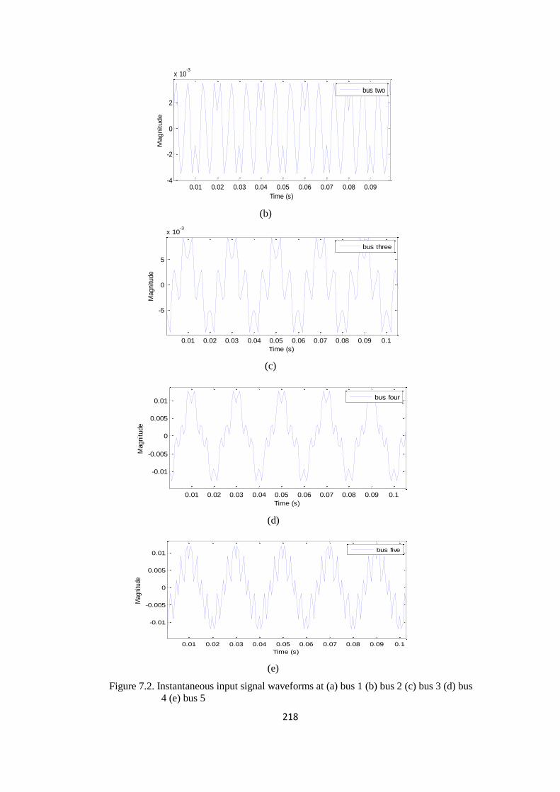
218
0.01 0.02 0.03 0.04 0.05 0.06 0.07 0.08 0.09-4
-2
0
2
x 10-3
Time (s)
Magnitude
bus two
(b)
0.01 0.02 0.03 0.04 0.05 0.06 0.07 0.08 0.09 0.1
-5
0
5
x 10-3
Time (s)
Magnitude
bus three
(c)
0.01 0.02 0.03 0.04 0.05 0.06 0.07 0.08 0.09 0.1
-0.01
-0.005
0
0.005
0.01
Time (s)
Magnitude
bus four
(d)
0.01 0.02 0.03 0.04 0.05 0.06 0.07 0.08 0.09 0.1
-0.01
-0.005
0
0.005
0.01
Time (s)
Mag
nitu
de
bus five
(e)
Figure 7.2. Instantaneous input signal waveforms at (a) bus 1 (b) bus 2 (c) bus 3 (d) bus
4 (e) bus 5

219
The above results shows that the natural sampled pulse-width modulation with
harmonic injection in the nodal signal produces only fundamental harmonic defined by
modulation index and dc-link voltage within the baseband harmonics range and injected
harmonics with magnitude dependent on Mh and DC-link.
The signal in Fig. 7.2 contains the fundamental component, 3rd
, 5th and 7
th harmonics.
According to the waveforms in Fig. 7.2, the signal swell disturbance of fundamental
component starts at the bus three (PQ bus), the 3rd
and the 5th harmonic disturbance
become more significant at bus four (PQ bus), whilst the 3rd
, 5th and 7
th harmonic appear
more disturbance at bus five (PQ bus). Hence, the information of fundamental
frequency and harmonic components can easily be obtained from the waveforms in Fig.
7.2.
Figure 7.3 shows the phase current characteristic corresponding to the ac current
obtained by harmonic voltage injection technique. Figure 7.4 depicted the load bus
current obtained from the real power, reactive and bus voltage Newton’s power flow.
The ac voltages are available from ac power flow as shown in Figure 7.5. All currents
and voltages in this circuit are non-sinusoidal also for the load currents. Of particular
interest are the currents through the capacitive and the inductive elements of the multi-
terminal network. In this case the line current at the buses are non-sinusoidal but it is
likely that these are due to the harmonic currents injected.
0 0.05 0.1 0.15 0.2 0.25-0.4
-0.2
0
0.2
0.4
Time (s)
Curr
ent
(A)
ia(t)
ib(t)
ic(t)
Figure 7.3. Three Phase Current Waveform

220
0 0.05 0.1 0.15 0.2 0.25-0.4
-0.2
0
0.2
0.4
Time (s)
Curr
ent
(A)
curb3
curb4
curb5
Figure 7.4. Load bus current waveform
0 0.05 0.1 0.15 0.2 0.25-6
-4
-2
0
2
4
6
Time (s)
Voltage (
V)
Figure 7.5. Voltage control bus waveform
7.5. Harmonic Power Flow: Test Case 2
Simulation studies of the proposed modular multi-level MTDC system for integrating
two self-excited induction generators (SEIG) based wind farms (WFs) with the remote
grids (oil and gas platforms). The system configuration and parameters are shown in
Fig. 7.1. Two SEIG-based wind farms (WFs) are both rated at 200MW. The wind power
is collected by aggregated WFs, and then finally transmitted to three remote platforms
grids located 200km, 150km and 100km respectively away by VSC-HVDC links.
The proposed model for the five bus multi-terminal VSC-HVDC is implemented using
MATLAB and the simulation parameters are as follows:
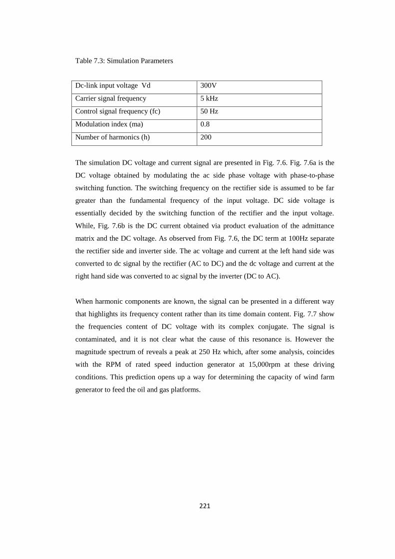
221
Table 7.3: Simulation Parameters
Dc-link input voltage Vd 300V
Carrier signal frequency 5 kHz
Control signal frequency (fc) 50 Hz
Modulation index (ma) 0.8
Number of harmonics (h) 200
The simulation DC voltage and current signal are presented in Fig. 7.6. Fig. 7.6a is the
DC voltage obtained by modulating the ac side phase voltage with phase-to-phase
switching function. The switching frequency on the rectifier side is assumed to be far
greater than the fundamental frequency of the input voltage. DC side voltage is
essentially decided by the switching function of the rectifier and the input voltage.
While, Fig. 7.6b is the DC current obtained via product evaluation of the admittance
matrix and the DC voltage. As observed from Fig. 7.6, the DC term at 100Hz separate
the rectifier side and inverter side. The ac voltage and current at the left hand side was
converted to dc signal by the rectifier (AC to DC) and the dc voltage and current at the
right hand side was converted to ac signal by the inverter (DC to AC).
When harmonic components are known, the signal can be presented in a different way
that highlights its frequency content rather than its time domain content. Fig. 7.7 show
the frequencies content of DC voltage with its complex conjugate. The signal is
contaminated, and it is not clear what the cause of this resonance is. However the
magnitude spectrum of reveals a peak at 250 Hz which, after some analysis, coincides
with the RPM of rated speed induction generator at 15,000rpm at these driving
conditions. This prediction opens up a way for determining the capacity of wind farm
generator to feed the oil and gas platforms.
222
10 20 30 40 50 60 70 80 90 100
-200
0
200
Magnitude
Vdc
10 20 30 40 50 60 70 80 90 100
-80
-60
-40
-20
0
20
40
Frequency(Hz)
Magnitude
Idc
Figure 7.6. DC voltage and current at switching frequency
50 100 150 200 250 300 350 400 450 5000
0.5
1
1.5
2
2.5
x 104
Frequency(Hz)
Voltage M
agnitude (
V)
Figure 7.7. Frequency Content of Vdc with its complex conjugate
Figure 7.8 is input ac current (Iin) obtained via modulating the DC current with the
phase-to- phase current switching function. To ensure a sinusoidal input current, it is
mandatory to include a second active switching state of the input stage in the
modulation scheme.

223
10 20 30 40 50 60 70 80 90 100
-1
-0.5
0
0.5
1
Curr
ent
Magnitude
Frequency(Hz)
Figure 7.8. Input Current
10 20 30 40 50 60 70 80 90 100-20
0
20
40
Frequency(Hz)
Voltage M
agnitude
Vcap1
Vcap2
Vcap3
10 20 30 40 50 60 70 80 90 100
0
50
100
Curr
ent
Magnitude
Icap1
Icap2
Icap3
Figure 7.9. (a)Capacitor voltage (b) Capacitor current
Figure 7.9 depicts the capacitor voltage and current which are across the individual
converter. The capacitor voltage is directly proportional to the equivalent capacitor
impedance and DC current with the DC term. The capacitor current is the sum of the
individual node current and the DC current.
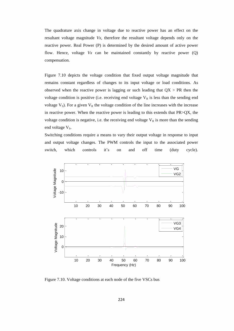
224
The quadrature axis change in voltage due to reactive power has an effect on the
resultant voltage magnitude Vx, therefore the resultant voltage depends only on the
reactive power. Real Power (P) is determined by the desired amount of active power
flow. Hence, voltage Vx can be maintained constantly by reactive power (Q)
compensation.
Figure 7.10 depicts the voltage condition that fixed output voltage magnitude that
remains constant regardless of changes to its input voltage or load conditions. As
observed when the reactive power is lagging or such leading that QX > PR then the
voltage condition is positive (i.e. receiving end voltage VR is less than the sending end
voltage VS). For a given VR the voltage condition of the line increases with the increase
in reactive power. When the reactive power is leading to this extends that PR>QX, the
voltage condition is negative, i.e. the receiving end voltage VR is more than the sending
end voltage VS.
Switching conditions require a means to vary their output voltage in response to input
and output voltage changes. The PWM controls the input to the associated power
switch, which controls it’s on and off time (duty cycle).
10 20 30 40 50 60 70 80 90 100
-10
0
10
Voltage M
agnitude
VG
VG2
10 20 30 40 50 60 70 80 90 100
0
10
20
Frequency (Hz)
Voltage M
agnitude
VG3
VG4
Figure 7.10. Voltage conditions at each node of the five VSCs bus

225
The instantaneous real and reactive powers of the respective bus network are depicts in
Fig. 7.11. From the simulation results, the system reaches stable state at rectifier stage,
i.e., from AC to DC before starting HVDC. In Fig.7.11a, wind farm system supplies 100
MW through the HVDC-VSC initially; before reaching node one, the decreased power
output of VSC-HVDC are balanced by HVDC, operating at 50 kV eventually. DC
voltage and current of HVDC rectifier side reaches the reference values of 1.0 p.u. and
0.2 p.u. respectively, as represented in Fig. 7.13.
10 20 30 40 50 60 70 80 90 100-300
-200
-100
0
100
Frequency (Hz)
Magnitude
10 20 30 40 50 60 70 80 90 100
-100
-50
0
50
100
Frequency (Hz)
Magnitude
(a)
(b)
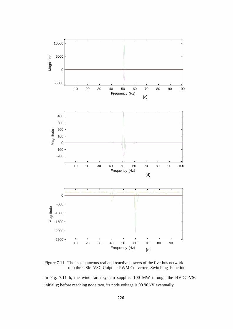
226
10 20 30 40 50 60 70 80 90 100
-5000
0
5000
10000
Magnitude
Frequency (Hz)
10 20 30 40 50 60 70 80 90 100
-200
-100
0
100
200
300
400
Frequency (Hz)
Magnitude
10 20 30 40 50 60 70 80 90-2500
-2000
-1500
-1000
-500
0
Frequency (Hz)
Magnitude
Figure 7.11. The instantaneous real and reactive powers of the five-bus network
of a three SM-VSC Unipolar PWM Converters Switching Function
In Fig. 7.11 b, the wind farm system supplies 100 MW through the HVDC-VSC
initially; before reaching node two, its node voltage is 99.96 kV eventually.
(c)
(d)
(e)

227
Figures 7.11c, 7.11d and 7.11e shows the instantaneous real and reactive powers of the
platforms bus (load bus). The platforms node voltages are 74 kV, 72 kV, and 40 kV
respectively.
In this simulation, the AC/DC rectifiers of the network have been subjected to three-
phase modular multi-level behaviour of the multi-terminal HVDC-VSC network. It can
be seen in Figure 7.11 that the three SM-converters have a high magnitude of
instantaneous real and reactive power comparable to five SM-converters as depicted in
Figure 7.12. This improves the real and reactive power profiles. Also noticeable is that
the ten SM-converter as shown in Figure 7.13 has significant improvement on the power
quality of the whole system.
Active and reactive power shown in Figure 7.11-7.13, are handled by all nodes. The
nodes network has enough reserve to take additional power to account for any
mismatches in the DC network as shown in the figures below. Figure 7.11-7.13 shows
active power being transferred to the DC via the AC side.
10 20 30 40 50 60 70 80 90 100
-200
-150
-100
-50
0
50
100
Frequency (Hz)
Magnitude
10 20 30 40 50 60 70 80 90 100
-100
-50
0
50
100
150
Frequency (Hz)
Magnitude
(a)
(b)
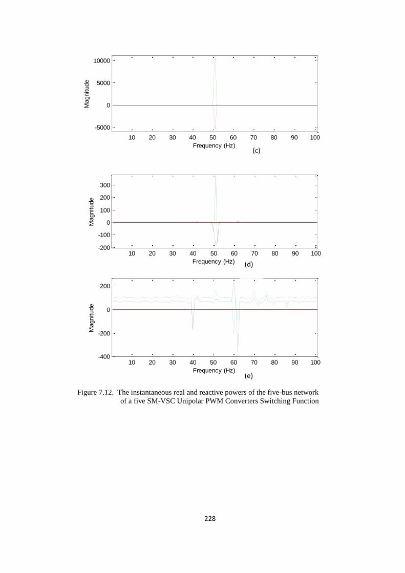
228
10 20 30 40 50 60 70 80 90 100
-5000
0
5000
10000
Magnitude
Frequency (Hz)
10 20 30 40 50 60 70 80 90 100-200
-100
0
100
200
300
Frequency (Hz)
Magnitude
10 20 30 40 50 60 70 80 90 100-400
-200
0
200
Frequency (Hz)
Magnitude
Figure 7.12. The instantaneous real and reactive powers of the five-bus network
of a five SM-VSC Unipolar PWM Converters Switching Function
(c)
(d)
(e)

229
10 20 30 40 50 60 70 80 90 100
-200
-100
0
100
200
Frequency (Hz)
Magnitude
10 20 30 40 50 60 70 80 90 100-300
-200
-100
0
100
200
300
Frequency (Hz)
Magnitude
10 20 30 40 50 60 70 80 90 100-1
-0.5
0
0.5
1
1.5
2
x 104
Magnitude
Frequency (Hz)
(a)
(b)
(c)

230
10 20 30 40 50 60 70 80 90 100
-200
0
200
400
Frequency (Hz)
Magnitude
10 20 30 40 50 60 70 80 90 100-600
-400
-200
0
200
Frequency (Hz)
Magnitude
Figure 7.13. The instantaneous real and reactive powers of the five-bus network
of a ten SM-VSC Unipolar PWM Converters Switching Function
The full-scale power converter presented in Figure 7.1 typically can include a generator
bridge, which in normal operation operates as an active rectifier to supply power to a
DC-link circuit. The wind farm-side converter (rectifier) can have suitable topology
based on full-bridge converters fully controlled and regulated using pulse-width
modulation. The DC output of the generator bridge to the DC terminals of a network
bridge through the DC-link circuit. The smoothing reactor is selected to avoid resonance
in the DC side at low order harmonic frequencies like 100 or 150 Hz. This is important
to avoid the amplification effect for harmonics originally from the AC system, like
negative sequence and transformer saturation.
The grid-side converter normally operates as a PQ bus and is also considered within the
analysis as an inverter. The network bridge can have a topology as presented in Figure
6.1 fully controlled using the pulse-width modulation strategy. The AC output voltage
of the grid-side converter is filtered and supplied to the fixed frequency supply network
via a step-up transformer.
(d)
(e)
231
A good criterion of harmonic resonance issue is the capacity of the MMC which are
shown for all considered cases. The solutions of the frequency response equations
regarding the stability of the system are shown in Figs. 7.11 to 7.13. These distorted
signals contains just one resonant argument and not damagerous, just a little aggravating
will lead to realistic power quality.
Figure 7.11 shows the effect of the three-SM on the multi-terminal MMC-HVDC-VSC
for harmonic elimination and stability case. It can be seen from the figure that
maximum steady state magnitude occurs when harmonic resonance equal 2 kHz except
for Fig. 7.11c, 7.11d, and 7.11e that appears at 1 kHz. It is clear that power quality is
achieved after harmonic resonance at 2 kHz.
Figure 7.12, shows the power quality results for the five-SM case. Also, it can be seen
that from Fig. 7.12, that the last resonance that was observed in three-SM case has been
eliminated or shifted backward. Clean evidence that more power quality is achieved as
the SM converter increase.
Figure 7.13, illustrates the simulation for ten-SM, as shown the resonance is greatly
reduced and is no longer providing the strong harmonic content. More also, all samples
resonance are completely eliminated, which maybe excited by the out of balance
harmonics.
7.6. Conclusions
A power flow model of the modular multi-level VSC is presented, it is seen that the
modified load flow equations improve system performance.
In interconnected power systems different power quality problems exist. The harmonic
voltage problem has a significant effect on voltage levels at each bus. In this thesis, the
voltage levels at each bus for different types of loads are observed. The low voltage
magnitude at all bus can be improved by introducing modular multi-level VSC device at
the node locations. In this five bus system the desired location of VSC device is, at
which all bus low voltage level is maintained. The performance of modular VSC to
improve voltage bus with different type of loads is observed and also the effect of
different locations of shunts compensators on voltage magnitude is observed.

232
Instantaneous power theory gives a piecemeal approach in analysis and control of the
active and reactive components of the harmonic load and introduces the active power
filter for appropriate corrective measure for the total harmonic distortion for
improvement of the power quality as per the scheduled standards. Energy efficient
power supplies incorporating active power supplies shall govern the future in the
electrical power quality standardizations.
7.7. References
[1] R.Balamurugan and G.Gurusamy “Harmonic Optimization by Single Phase
Improved Power Quality AC-DC Power Factor Corrected Converters",
International Journal of Computer Applications, Volume 1, No. 5, 2010.
[2] J.Conde-Enriques, J.S.Benites-Read, J.L. Duran-Gomez and J.O.Pachecho-Sotelo J
“Three-phase six-pulse buck rectifier with high quality input waveforms” 1999
IEE Proceedings-Electric Power Applications Vol. 146.
[3] W.A.A. De Doncker Rik, Deepakraj M.Divan, and M.H. Kheraluwala. “A Three-
Phase Soft-Switched High-Power-Density DC/DC Converter for High-Power
Applications”. IEEE Transactions on Industry Applications, 1991.
[4] D.Czarkowski and M.K.Kazimierczuk. “Spice Compatible Averaged Models of
PWM Full-Bridge Dc-Dc Converter”. In Industrial electronics, control,
instrumentation, and automation, 'Power electronics and motion control'
Proceedings of the 1992 inter- national conference, 1992.
[5] T.Ming-Tsung and W. I. Tsai, “Analysis and Design of Three-Phase AC-to-DC
Converters with High Power Factor and Near-Optimum Feed forward” IEEE
Transactions On Industrial Electronics, Vol. 46, No. 3, June 1999.
[6] Y.Jiang-Hafner, H.Duchen, M.Karlsson, L.Ronstrom and B.Abrahamsson,
“HVDC with Voltage Source Converters .A Powerful Standby Black Start
Facility”.IEEE PES T&D Conference, April 2008.
[7] M.P. Bahrman and B.K. Johnson, “The ABCs of HVDC Transmisson
Technologies”. IEEE Power & Energy magazine, March/April 2007, p32~44.
[8] W. Lu, “Simultaneous Inter-Area Decoupling and Local Area Damping by
Voltage-Source HVdc”. 2001 IEEE.
[9] R.Critchley, “The role of HVDC & FACTS technologies to enhance the
utilisation of existing transmission networks”. AREVA T&D Technology Centre,
March 2009.

233
[10] M.Khederzadeh, “Power Quality Aspects of Different Control Schemes of Back-
to-Back Converters Interfacing Utility-Grid to Microgrid”. C I R E D on
Electricity Distribution, June 2011.
[11] B.Singh, B.N. Singh, A. Chandra, K. Al-Haddad, A.Pandey, and P.D.P.Kothari,
"A Review of Single- Phase Improved Power Quality AC-DC Converters", IEEE
Transaction on Industrial Electronics, Vol. 50, No. 5, pp. 962-981, USA,
October, 2003.
[12] A.Pandey, and P.D.P. Kothari, "A Review of Three- Phase Improved Power
Quality AC-DC Converters", IEEE Transaction on Industrial Electronics, Vol.
51, No. 3, pp. 641-660, USA, 2004.
[13] E. López-Luis, M. A. García-Domínguez, and D. Ruiz-Vega, “The Effect of
Improved System Modelling in the Continuation Power Flow Method”. 2007
IREP Symposium- Bulk Power System Dynamics and Control - VII, Revitalizing
Operational Reliability.
[14] B.Poudel, V.Cecchi, “Harmonic Power Flow Using Multi-Segment Frequency-
Dependent Transmission Line Models”. IEEE 2013.
[15] M.Robert and D.Vecchio, “Multiterminal Three Phase Transformer Model with
Balanced or Unbalanced Loading”. IEEE Transactions on Power Delivery, Vol.
23, No. 3, July 2008
[16] R.Stoicescu, K.Miu, C. O. Nwankpa, D.Niebur, and Xiaoguang Yang, “Three-
Phase Converter Models for Unbalanced Radial Power-Flow Studies” IEEE
Transactions on Power Systems, Vol. 17, No. 4, November 2002.
[17] P.W.Lehn,”Direct Harmonic Analysis of the Voltage Source Converter” IEEE
Transactions on Power Delivery, Vol. 18, No. 3, July 2003.
[18] M.Rashid “Power Electronics: Circuits, Devices, and Applications”, 3rd Edition,
Prentice Hall New Jersey, USA, 2004.
[19] P.Marketos, A.J.Moses and J.P.Hall,“Effect of DC Voltage on AC Magnetisation
of Transformer Core Steel”. Journal of ELECTRICAL ENGINEERING, Vol 61.
No 7/s, 2010, 123-125
[20] T. M. Blooming, and D.J. Carnovale, ”Capacitor Application Issues”
[21] H.P.Tiwari ,”Capacitor Rating Selection for Voltage Sag Compensation in DVR
System” International Journal of Innovation, Management and Technology, Vol.
1, No. 3, August 2010
[22] G. Andersson, “Modelling and Analysis of Electric Power Systems”. Power Flow
Analysis, Fault Analysis, Power Systems Dynamics and Stability. ITET ETH
Z¨urich

234
CHAPTER 8
8. Conclusions and Further Works
8.1. Conclusions
Harmonic power system analysis, particularly at the planning stage, has become
increasingly important as it constitutes a powerful tool for the adequate assessment and
enhancement of power quality, and the impact of harmonic distortion upon system
components. Accurate representation of power network component nonlinearities and
the interaction with other electric network components is of fundamental importance in
rigorous harmonic studies.
In this thesis, computer simulations to ascertain harmonic resonance performance of
high voltage models under steady-state conditions have been investigated using
improved cable models. The study shows that an accurate underground/subsea cable
model and its mathematical equations could be a strong tool for predicting the harmonic
resonance conditions of power cable in a transmission system. The simulation results
shows that the frequency response depends on design lumped parameters such as: the
cable length, capacitive and inductive components. The analysis estimates that the
potential risks on the voltage and current harmonic amplifications could be avoided or
controlled using accurate modelling.
For this purpose, the proposed Bessel function model stands out in investigating the
frequency response and harmonic resonances of the system. The results obtained are
validated with the simulation results of an approximation model using MATLAB. The
two models results show very good agreement as anticipated. This study further
contributes towards an insight that underground/subsea cable is influenced by harmonic
resonance in transmission systems. It implies that the cable model needs to be carefully
assessed in order to represent the harmonic behaviour of the transmission systems. Also,
to understand the harmonic behaviour and harmonic distortion, the aspect of power
losses must be considered as this is critical to the design of offshore power transmission
systems.
235
A comprehensive model for the periodic, steady-state operation of VSCs was presented
in this thesis. Switching functions based on complex Fourier series are used very
effectively to represent the operation of the VSC. The modelling approach applies to a
wide range of VSC configurations.
The MMC based VSC converter technology is expandable to high level waveforms. Its
large number of sub-modules, capacitors in each phase-leg and combined with a proper
accurate algorithm regulates the voltage of the sub-module capacitors. With these
flexibilities the converter structure operates well under unipolar-PWM voltage
switching principle that results in high quality waveforms while maintaining the low
switching frequency of the SM switches.
Based on the configuration of the MMC, a phase-shifted modulation scheme is
proposed for the unipolar-PWM carrier. It provides high quality waveforms while
generating different number of levels in the output voltage waveforms.
Cancellation theory and the notion of resultants can be used to cancel the lower and
higher order harmonics in a modular multilevel converter. This method is expected to
have widespread application as most modular multilevel converters do not have dc
sources that are exactly equal.
The VSC model was used as a building block to assemble harmonic domain models for
the VSC-HVDC back-to-back and for the VSC-HVDC transmission station. The model
of the VSC-HVDC transmission station works well with an accurate model of the cable
since both models are in the frequency domain. Possible applications of the frequency
domain models presented in the thesis are: harmonic propagation studies, resonance
prediction and harmonic stability analysis.
A new radial oil and gas platform model fed by an offshore wind farm, connected
through VSC-HVDC transmission system was studied. The main advantage of this
model is that, it is built with Static Var Compensator (SVC), whose compact
components are the capacitor and inductor. This compensator brought a new solution
technique to a power quality problem on the platform. Low harmonic voltages and
reactive power support was achieved through this technique. In this application, the
SVC is not a device intended to permit the full, steady state loading of the transmission
line to its capacity; it is a device intended to improve power quality. In this model SVC

236
draw high interest with power quality because of its harmonic impact on the system
resonance and voltage regulation.
A new harmonic power flow strategy of the VSC-HVDC system for providing a high-
quality supply to oil and gas platforms are proposed. In the proposed strategy, a
switching function technique and harmonic injection are implemented in the stations of
the VSC-HVDC. The motivation for choosing this strategy is to exploit the harmonic
propagation decreasing the frequency of the VSC-HVDC output voltage when needed.
Thus, a momentary surplus of harmonic magnitude reduction is achieved.
The increasing interest in integrating renewable electricity from remotely located energy
sources, such as offshore wind power, is promoting the development of high-voltage
multi-terminal DC networks, which offer several advantages when compared with
standard high-voltage AC networks. In view of this, the VSC-HVDC technology stands
out as the most promising solution. However, several regulatory as well as technical
challenges must be addressed before such multi-terminal DC (MTDC) systems can be
established.
In addition, the thesis has described the steady-state models of the main components in
an MTDC network. A novel harmonic power flow strategy has been presented to study
the DC power flow. The HPF strategy was analysed in combination with a switching
function algorithm that minimizes the MTDC system losses. A total of five bus case
studies have been conducted, via simulations in MATLAB. The simulation results
demonstrate that the proposed power flow strategy is capable of generating power
quality and safely controlling the DC power flow. Furthermore, the HPF strategy has
fast communications capability and can handle the power flow in complex DC
networks.
Oil and gas networks with VSC-HVDC and internal modular multilevel DC network
has been proven to enhance drive systems mounted on the DC-bus, the incoming energy
from the wind farm delivered energy to the individual DC-bus via aggregated induction
generator and slightly decreasing the frequency of the VSC output voltage.
There is a higher flexibility in this approach, in that the frequency reduction can be
applied selectively only to those machines that are not sensitive, while the stored energy
through the DC-bus can be used to keep the critical ones on line. Further improvement
can be obtained by connecting some additional storage to the common DC-bus. This can

237
result in a more cost-effective solution than increasing the storage (capacitor size) at
each DC-bus of the individual drive system, as it is done in the traditional AC solution
to increase the ride-through capability of the drive.
Further simulation results show that the developed harmonic control system was able to
keep the voltage and frequency variations within the grid code even during large
disturbances. We can conclude that the system handles variations in the load very well
and that the system configuration studied in this thesis is regarded as a feasible way of
integrating oil and gas platforms and offshore wind power to the onshore grid. However
more detailed studies are recommended including short circuit analysis.
The HPF program developed in MATLAB environment has been tested on several
nonlinear loads such as: VSC, rectifier, and gives satisfactory results for the simulations
performed confirming the relevance of this code. The results were consistent and show
the influence of higher harmonics on power losses in electrical networks. And we have
confirmed the possibility to analyse other nonlinear loads with this computer code HPF
generating harmonics in power systems.
8.2. Recommendations
Considering the benefit-to-cost ratio, based on our multi-terminal model network, an
HVDC-VSC connection to the oil and gas platform network will indeed be most
profitable to oil and gas companies. As can be seen from the analysis connection will be
cost-effective up to thousands of MW renewable generation. For higher generation, a
multi-terminal connection to different platforms is preferred. Also, as the emission price
goes higher, the net benefit of multi-terminal connection to the grid becomes more
attractive.
The harmonic problems are very high; the cases in which they do occur can result in
decreasing power system reliability. An understanding of the causes, potential effects
and mitigation means for harmonics can help to prevent harmonic related problems at
the design stage and reduce the probability of undesired effects occurring on operation.
It should be kept in mind that if the harmonic producing loads are small in relation to
the total plant load, then harmonics are not an issue. When the non-linear loads become
a substantial portion of the total load, it becomes worthwhile to give some consideration
to harmonics. In these cases, harmonic modelling analysis is recommended to predict

238
harmonic levels and identify potential resonance problems regardless of the rectifier
pulse number.
8.3. Further Work
The VSC-HVDC concept includes another development in future the extruded polymer
VSC-based HVDC Cable. The technology will shift High Voltage AC cables from
paper insulated to extruded polymer cables which will be replicated in HVDC cables.
The cable could be designed with a 300mm copper conductor surrounded by a strong
polymeric insulating material. The water sealing of the cable could be design with a
seamless layer of extruded lead and finally two layers of armouring steel wire in counter
helix for the mechanical properties of the cable. Their strength and the flexibility will
make these cables suited for severe installation conditions and deep waters oil and gas
platforms. The model is compatible with active filtering that will fight harmonic
distortion and resonance conditions.
Space and weight are also scarce resources on offshore installations. However, the use
of small filters makes the VSC based HVDC concept relatively compact and
lightweight. The offshore environment is also very tough with salt and humid air
imposing severe requirements on the choice of materials and surface treatment. To this
end, the investigation of harmonic behaviour of this cable is required, the assessment is
imperative to enable design engineers consider actual harmonic mitigation approaches.
The power quality and the accuracy of the harmonic resonance mode analysis need to be
verified with real life measurements in power systems. The harmonic resonance mode
analysis detects the parallel resonances in a power system (i.e. the major resonance
problem), but it could be completed to detect the series resonances as well. The role and
the physical meaning of the participating factors need further investigation.
A systematic and power quality automatic calculation algorithm based on the harmonic
modal analysis would facilitate the resonance analysis of the distribution and
transmission networks and help to identify the optimal locations for active filters.
Further work also, may involve the modular multi-level inverter containing series of
components each with its own role. The main components are the IGBT units which
form the three phases of the inverter. Each phase should contain tens of IGBT units
239
allowing up to 13 levels per phase and 17 levels. A unit can handle voltages up to 600 V
but 800 V can also be achieved if the units are pushed at higher voltages. The system
components are: IGBT s ; Current sensors; Voltage sensors; Contactors and DC Power
Supply.
Furthermore, future work involves building a small-scale version of the represented
MTDC network in a laboratory, testing the harmonic power flow in a real-time
environment, and assessing the effect of direct voltage measurement errors on the DC
load flow obtained with the proposed strategy.
Integration of photovoltaic (PV) and wind based renewable energy systems, main grid
feeding both onshore and offshore oil and gas installations forms part of the future
work. To undertake the study an aggregated current source model shall be proposed for
the photovoltaic inverter systems and wind farm based on measurement data from
available literature and the relevant international standards. A typical medium voltage
(MV) and low voltage (LV) distribution feeder including oil and gas production field
load arrangements is ideal for the study. The flexible harmonic model for the grid, the
cables, linear loads, nonlinear loads and the rectifiers and inverters (harmonic current
capacitance and conductance) are to be used to simulate the behaviour of the proposed
micro grid topology composed of both linear and nonlinear loads and grid photovoltaic
(PV) and wind farm (WF) systems. The harmonic currents injection at the point of
connection could be obtained at the output of a grid connected PV and WF systems.
Conventional harmonic modelling methods should be applied to determine harmonic
emissions and resulting harmonic voltage levels for various penetration levels of
photovoltaic inverter systems and wind farm based VSC-HVDC. Based on this study, a
recommendation should be made for acceptable penetration levels to limit the harmonic
impact of grid connected PV inverter systems and WF VSC-HVDC systems. The
distribution network considering distributed generation (DG), the model has to be
modelled to analyze the effects of wind farms and PV solar installations ground current
contribution to the network. The DG is based on capacitive coupling models of a 100
MW PV solar installation and a 200 MW wind farm respectively. This distribution
network feeds six loads through a multi-terminal ring topology. These loads are
connected to bus 1, 2, 3, 6, 7 and 8 with a rated power of 500+ j 55 kVA each.

240
Appendix
Appendix A1
International Harmonic Standards
The purpose of imposing strict limits on the harmonics emissions is to ensure that the
current and voltage distortions at the PCC are kept sufficiently low. Thus, the other
customers connected at the same point are not disturbed. The international standards
related to harmonic distortion limits can be classified as follows:
A. Standards specifying limits for individual nonlinear equipment
IEC 61000-3-2, which specifies the current harmonic limits for low voltage
equipment that has an input current less than 16 A.
IEC 61000-3-12 , which specifies the current harmonic limits for equipment
that has an input current between 16A and 75A
IEC 61800-3, which specifies the electro-magnetic compatibility (EMC)
requirements of the adjustable speed drive systems
As noticed, the above standards are for small rating and low voltage harmonic loads
only. In addition, the above standards do not set limits on the overall distribution
network.
B. Standards specifying limits for electrical networks
IEEE 519-1992, this document introduces many useful recommended practices
for harmonics control in electrical networks. This document is widely used in
the industrial sector and many consultants/clients use the limits indicated in it
as contractual limits within their specifications.
IEC 61000-3-6, this specification performs an assessment of the harmonic
emission limits for distorting loads in medium voltage and high voltage power
systems.
Up till now, this specification is not widely used in the industrial sector because it is
rather new (published in 2008).
British engineering recommendation G5/4-1, this document provides some
helpful engineering recommendations for establishing the allowable harmonic
limits of the voltage distortions in the United Kingdom.
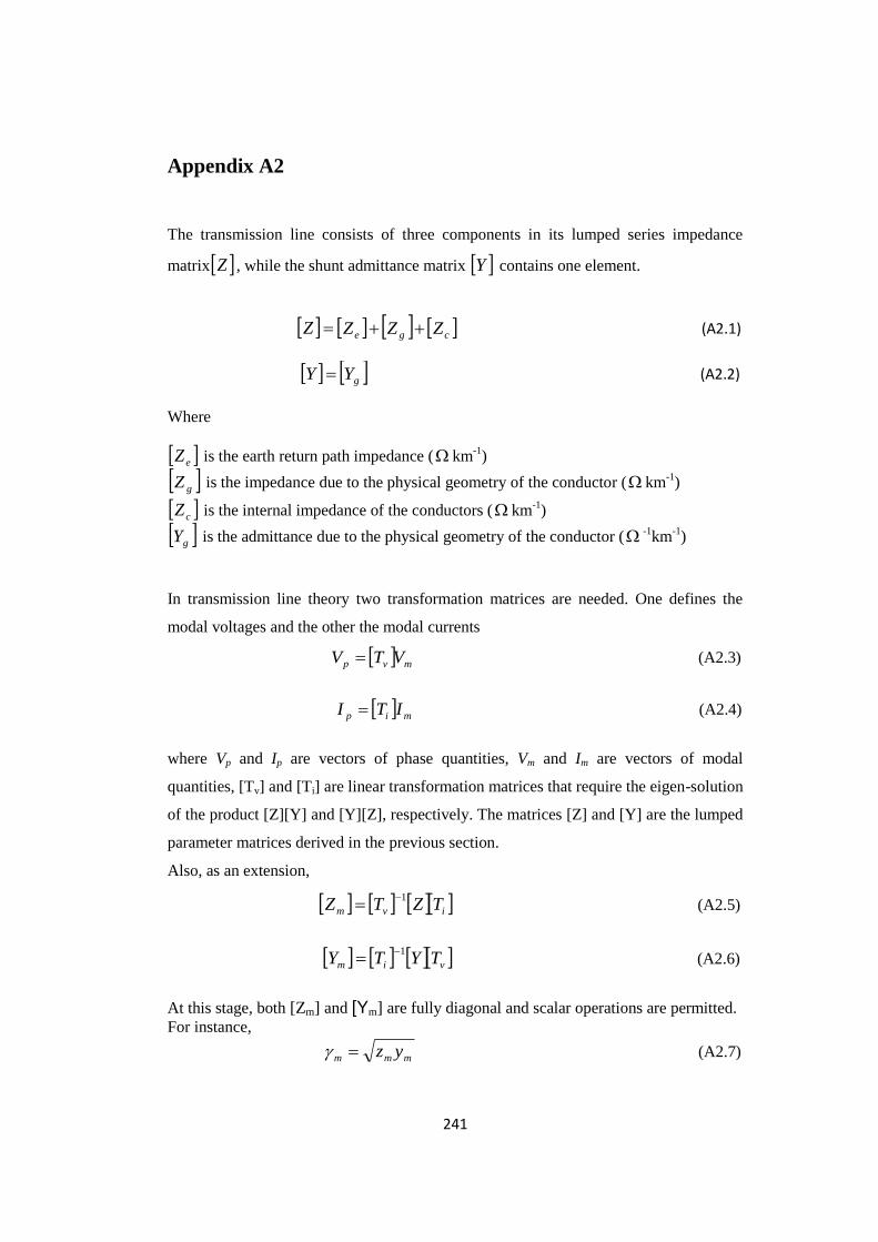
241
Appendix A2
The transmission line consists of three components in its lumped series impedance
matrix Z , while the shunt admittance matrix Y contains one element.
Z cge ZZZ (A2.1)
gYY (A2.2)
Where
eZ is the earth return path impedance ( km-1
)
gZ is the impedance due to the physical geometry of the conductor ( km-1
)
cZ is the internal impedance of the conductors ( km-1
)
gY is the admittance due to the physical geometry of the conductor ( -1km
-1)
In transmission line theory two transformation matrices are needed. One defines the
modal voltages and the other the modal currents
mvp VTV (A2.3)
mip ITI (A2.4)
where Vp and Ip are vectors of phase quantities, Vm and Im are vectors of modal
quantities, [Tv] and [Ti] are linear transformation matrices that require the eigen-solution
of the product [Z][Y] and [Y][Z], respectively. The matrices [Z] and [Y] are the lumped
parameter matrices derived in the previous section.
Also, as an extension,
ivm TZTZ1
(A2.5)
vim TYTY1
(A2.6)
At this stage, both [Zm] and [Ym] are fully diagonal and scalar operations are permitted.
For instance,
mmm yz (A2.7)
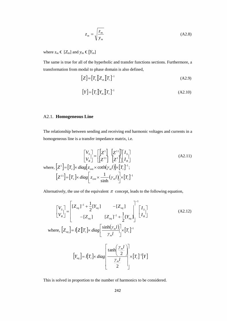
242
m
m
my
zz (A2.8)
where zm ϵ [Zm] and ym ϵ [Ym]
The same is true for all of the hyperbolic and transfer functions sections. Furthermore, a
transformation from modal to phase domain is also defined,
1 imv TZTZ (A2.9)
1 vmi TYTY (A2.10)
A2.1. Homogeneous Line
The relationship between sending and receiving end harmonic voltages and currents in a
homogeneous line is a transfer impedance matrix, i.e.
R
S
R
S
I
I
ZZ
ZZ
V
V111
111
(A2.11)
where, 11 coth
imomv TlzdiagTZ ;
111
sinh
1
imomv TlzdiagTZ
Alternatively, the use of the equivalent concept, leads to the following equation,
R
S
eqeqeq
eqeqeq
R
S
I
I
YZZ
ZYZ
V
V
1
1
1
][2
1][][
][][2
1][
(A2.12)
where,
1sinh
i
m
m
ieq Tl
ldiagTZlZ
YTl
l
diagTlY i
m
m
ieq
1
2
2tanh
This is solved in proportion to the number of harmonics to be considered.

243
When harmonic voltages rather than currents are to be injected (at the sending end) the
following equation is applies:
R
S
S
R
I
V
QS
RQ
I
V
][][
][][ (A2.13)
where, 1
)coth(
1
i
m
V Tl
diagTQ
1
0 )tanh(
immV TlzdiagTR
1
0
)tanh(1
vm
m
i Tlz
diagTS
When the aim of the analysis is to study the standing waves along the line or the
distribution of harmonic levels in a mesh of lines, it is necessary to obtain the line's
parameters in the form of admittance.
R
S
R
S
V
V
YY
YY
I
I
][][
][][111
111
(A2.14)
where, 1
0
1 )coth(1
vm
m
i Tlz
diagTY
= eqeq YZ2
11
1
0
11 )(sinh
11
vm
m
i Tlz
diagTY
= 1
eqZ
A2.2. Nominal versus Equivalent Pi Circuit Line Representation
There are two basic ways of representing transmission lines, namely by creating their
nominal Pi circuit or equivalent circuit. The first model is a simplified lumped
equivalent circuit where the whole length line resistance and reactance are concentrated
in the middle and shunt capacitance and conductance are concentrated at both ends see
Figure A2.1.
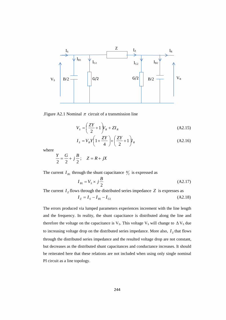
244
.Figure A2.1 Nominal circuit of a transmission line
RRS ZIVZY
V
1
2 (A2.15)
RRS IZYZY
YVI
1
241 (A2.16)
where
222
Bj
GY ; jXRZ
The current 1BI through the shunt capacitance 2B is expressed as
2
1
BjVI SB (A2.17)
The current ZI flows through the distributed series impedance Z is expresses as
11 GBSZ IIII (A2.18)
The errors produced via lumped parameters experiences increment with the line length
and the frequency. In reality, the shunt capacitance is distributed along the line and
therefore the voltage on the capacitance is VS. This voltage VS will change to VS due
to increasing voltage drop on the distributed series impedance. More also, ZI that flows
through the distributed series impedance and the resulted voltage drop are not constant,
but decreases as the distributed shunt capacitances and conductance increases. It should
be reiterated here that these relations are not included when using only single nominal
PI circuit as a line topology.
IS
B/2 VS VR B/2 G/2 G/2
IR Z
IB1 IG1 IG2
IB2
IZ

245
A2.3. Transmission line with distributed parameters
An actual transmission line representation with distributed impedance zdx and
admittance ydx is shown in Figure A2.2
Figure A2.2 Distributed parameters transmission line
The voltage and current change along the line can be express as
IZdx
dV (A2.20)
VYdx
dI Z (A2.21)
Differentiating for current and voltage we have
ZYVdx
Vd
2
2
(A2.22)
YZIdx
Id
2
2
(A2.23)
These equations express the wave propagation along a transmission line. Its
transformations express the rms values and phase angles of V and I at any point of the
line as
xCRRxCRR e
ZIVe
ZIVV
22
(A2.24)
IS
VS VR
IR Zdx
I+ I
IZ
Ydx V+ V V
dx x
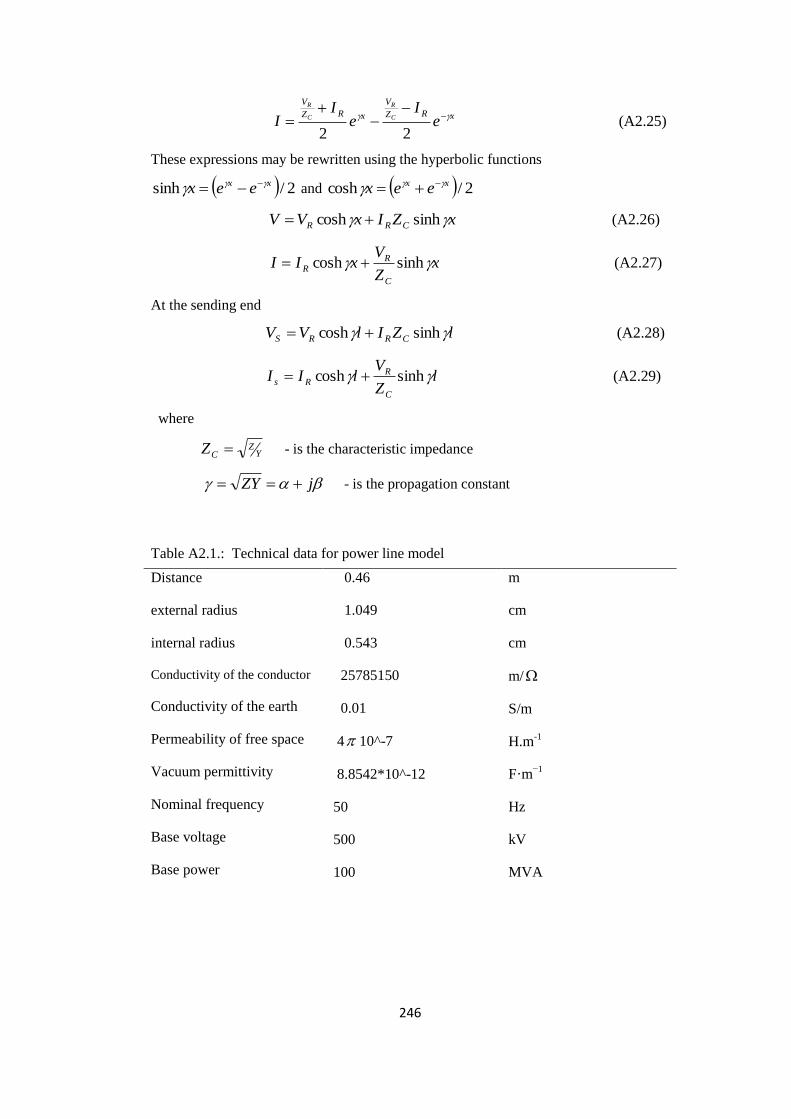
246
xRZ
V
xRZ
V
eI
eI
I C
R
C
R
22
(A2.25)
These expressions may be rewritten using the hyperbolic functions
2/sinh xx eex and 2/cosh xx eex
xZIxVV CRR sinhcosh (A2.26)
xZ
VxII
C
RR sinhcosh (A2.27)
At the sending end
lZIlVV CRRS sinhcosh (A2.28)
lZ
VlII
C
RRs sinhcosh (A2.29)
where
YZ
CZ - is the characteristic impedance
jZY - is the propagation constant
Table A2.1.: Technical data for power line model
Distance
external radius
internal radius
Conductivity of the conductor
Conductivity of the earth
Permeability of free space
Vacuum permittivity
Nominal frequency
Base voltage
Base power
0.46
1.049
0.543
25785150
0.01
4 10^-7
8.8542*10^-12
50
500
100
m
cm
cm
m/
S/m
H.m-1
F·m−1
Hz
kV
MVA

247
A2.4. Single Core Cables Parameters
The calculation of the per unit length parameters of a single-core cable, are based on
Fig. A2.3. The parameters equations, namely the series impedances Z and shunt
admittances Y are represented by matrices, which have a dimension [NxN], where N is
the number of conductors excluding the reference. [2x2] in the case of a single-core
cable. The phase voltages, vectors of dimension [Nx1], are reference to the ground
conductor.
In the case of [2x2], we consider two loops, in one loop the current is injected in the
core and returns by the sheath, whereas in the other the current is in injected on the
sheath and returns by the ground. We define loop currents and voltages, that ISint and
ISout, currents on the internal and external surfaces of the sheath, as well as loop voltage
V12 and V23, which are the core core-sheath and sheath-ground voltages. The sheaths
currents currents have physical substance only at high frequency, when the current
effectively flow on the conductors surfaces, but the loop quantities must always be
defined as means to evaluate phase quantities.
Figure A2.3 Transversal section of a single-core cable
A2.5. The Impedance and Admittance Matrices of a Cable System

248
Analysis of the impedance and admittance of a power cable is necessary for the
understanding of its characteristics [57]. Each cable has a cross section similar to the
type shown in Figure 4.15, representative of a typical high voltage (HV) underground
cable
Figure A2.4. Details of the construction of the 23-kV single-core cable
with three dielectric, operating frequency is 50Hz.
The impedance and admittance of a cable system are defined by the two matrix
equations,
IZ
dx
vd (A2.30)
vY
dx
Id (A2.31)
where
[Z] is the impedance square matrix
[Y] is the admittance square matrix
I is the vector current along the cable
v is the vector voltage along the cable
In general, the impedance and admittance matrices of a cable can be expressed in the
following forms
oCpi ZZZZZ (A2.32)
r6
r5
r4
r3
r2
r1
i
1
i2
i3
armor(ρ3,μ3 , 3)
Insulator 1
Insulator 2
Insulator 3

249
1.
PsY (A2.33)
ocpi PPPPP (A2.34)
where
[P] is the potential coefficient matrix
js
the matrices with subscript “i” are concerned with single core (SC) cable
the matrices with subscript “p” and “c” are concerned with pipe enclosure cable
the matrices with subscript “o” is concerned with cable outer media, that is air
space and earth
when a cable has no pipe enclosure, there exists no matrix with “p” and “c”
In the formulation of impedance and admittance of the cable system, the following
assumptions are necessary:
The displacement currents and dielectric losses are negligible.
Each conducting medium of a cable has constant permeability.
A2.6. Impedance
When an SC cable consists of a core, sheath and armour the impedance is given in the
following
[Z]=[Zi]+[Zo]+[Zskin]+[Zproximity] (A2.35)
where
[Zi] is the cable internal impedance diagonal matrix. A diagonal sub-matrix
expresses the self impedance matrix of an SC cable.
in
i
i
i
Z
Z
Z
Z
00
00
00
2
1
(A2.36)

250
Each submatrix, e.g. [Zi1] assembled along the leading diagonal is a square matrix of
two dimension representing the self impedances of cable i, by itself
iiii
iiii
sscs
sccc
ZZ
ZZZ11 (A2.37)
where
iiccZ = self impedance of the core of cables i
iiscZ =
iicsZ = mutual impedance between core and sheath of cable i
iissZ = self impedance of the sheath of cables i
[Zo] is the impedance matrix of the cable outer medium (ground return impedance) and
is given by
nnnn
n
n
ZZZ
ZZZ
ZZZ
Z
00201
02022012
01012011
0
(A2.38)
When the SC cable consists of a core, sheath and armour, the self-impedance matrix is
given by
aajsajcaj
sajssjcsj
cajcsjccj
ij
ZZZ
ZZZ
ZZZ
Z (A2.39)
where
Zccj = core self-impedance
Zssj = sheath self-impedance
Zaaj = armor self-impedance
Zcsj = mutual impedance between the core and sheath
Zcaj = mutual impedance between the core and armour
Zsaj = mutual impedance between the sheath and armour
When the SC cable consists of a core and sheath the self impedance is the matrix
reduced to a 2 x 2 matrix as given below and its equivalent circuit is as shown in Fig.
A2.4:
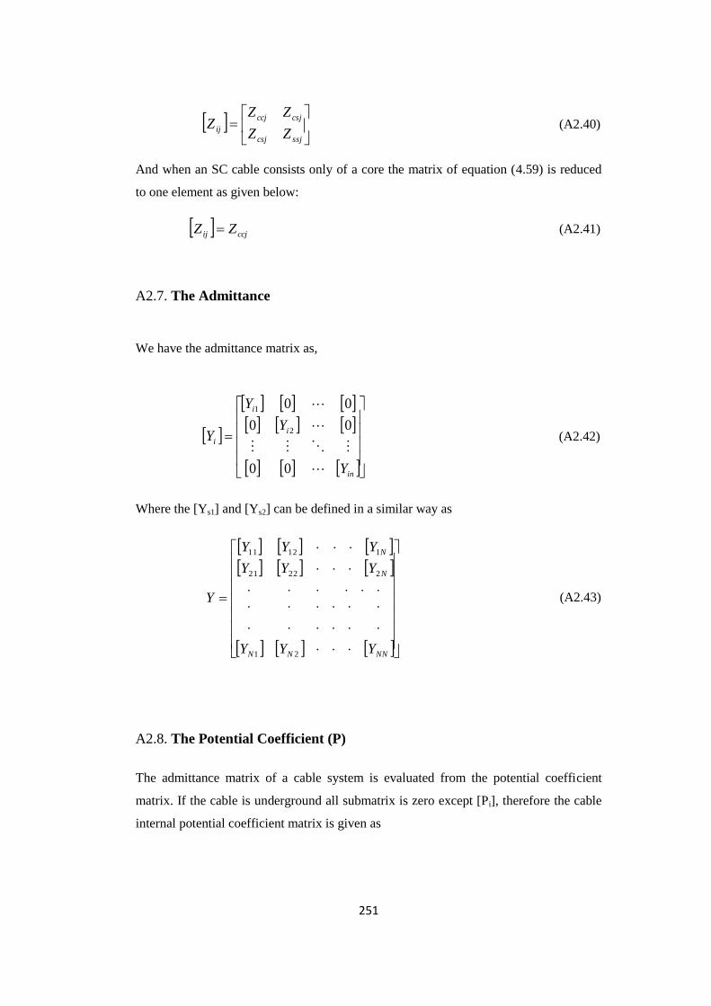
251
ssjcsj
csjccj
ij ZZ
ZZZ (A2.40)
And when an SC cable consists only of a core the matrix of equation (4.59) is reduced
to one element as given below:
ccjij ZZ (A2.41)
A2.7. The Admittance
We have the admittance matrix as,
in
i
i
i
Y
Y
Y
Y
00
00
00
2
1
(A2.42)
Where the [Ys1] and [Ys2] can be defined in a similar way as
NNNN
N
N
YYY
YYY
YYY
Y
21
22221
11211
(A2.43)
A2.8. The Potential Coefficient (P)
The admittance matrix of a cable system is evaluated from the potential coefficient
matrix. If the cable is underground all submatrix is zero except [Pi], therefore the cable
internal potential coefficient matrix is given as
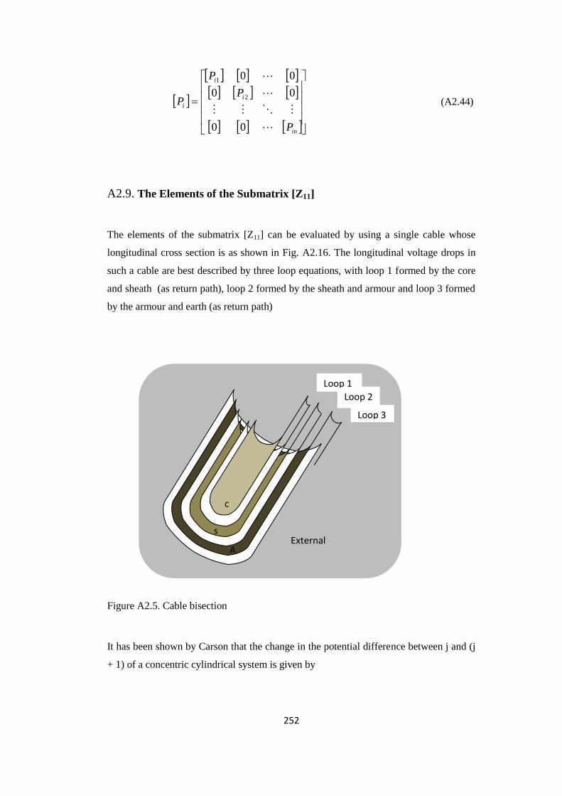
252
in
i
i
i
P
P
P
P
00
00
00
2
1
(A2.44)
A2.9. The Elements of the Submatrix [Z11]
The elements of the submatrix [Z11] can be evaluated by using a single cable whose
longitudinal cross section is as shown in Fig. A2.16. The longitudinal voltage drops in
such a cable are best described by three loop equations, with loop 1 formed by the core
and sheath (as return path), loop 2 formed by the sheath and armour and loop 3 formed
by the armour and earth (as return path)
Figure A2.5. Cable bisection
It has been shown by Carson that the change in the potential difference between j and (j
+ 1) of a concentric cylindrical system is given by
Loop 2
Loop 1
Loop 3
External
c
s
A

253
jJ jEEdx
dV 11
1 (A2.45)
where
Ej = longitudinal electric field strength of the outer surface of the conductor j
Ej + 1 = longitudinal electric field strength of the inner surface of conductor (j + 1)
The single-core trefoil type is expected to be more influenced by proximity effect
compared to the flat formations as shown in Fig. A2.5.
Figure A2.5 Subsea Cable Configurations
A2.10. Core Conductor
The core conductor aims to transmit the required electrical energy with low losses. The
high voltage conductor is made of copper (Cu) which has lower specific resistance
compared to aluminium (Al). Also, the conductor is often stranded in order to lower the
effective resistance caused by skin and proximity effect. When modelling such a non-
solid conductor, the resistivity is increased as presented in.
(a) Single-Core Trefoil Formation
Cable Structure.
(b) Three-Core Trefoil Formation
Cable Structure
(c) Single-Core Flat Formation
Cable Structure.

254
A2.11. Inner Insulation
The inner insulation aims at ensuring no electrical connection between the two current
carrying components of the cable, the conductor and the sheath. The SC screens are
placed between the insulation and the conductor and again between insulation and the
sheath. The purpose of the SC screens is to reduce the electrical stress in the inner
insulation and prevent formation of voids between either core conductor or sheath and
insulation due to bending of the cable or other mechanical stress. For flexible and
accurate modelling of the insulation and SC screens, the permittivity and thickness of
the insulation should be corrected according to the theory.
A2.12. Cable Sheath
The cable sheath aims at providing a metallic covering used as an electrostatic screening
as well as a earth return path for the cable’s charging current and a conduction path for
earth fault current in the event of a fault on the cable. As shown in Fig. A2.4, for XLPE
cables the sheath consists of several layers. The two conducting sheath layers, the wired
sheath layer and the laminated layer, are separated by a SC layer and are directly
connected together both at each junction and cable ends. The laminated layer is included
for water resistance. The two conducting layers are not touching each other in order to
protect the laminate from mechanical stress because of bending and for thermal
protection as the laminate cannot tolerate more than 180oC while the wired sheath layer
can be up to 250oC.
A2.13. Cable Armour
Armoured cable is the name given to any electrical cable constructed with a layer of
aluminium wire armour or steel wire armour. The armour sits below the sheath of the
cable to provide protection for the conductor and insulating layers. When an electrical
cable is required for use outside, burial or in direct subsea projects, it must have
mechanical protection. Aluminium wire armour or AWA, and steel wire armour or
SWA, provide such protection – as well as enabling the cable to withstand higher
pulling loads.

255
Steel Wire Armoured Cable is a hard-wearing mains electricity cable with class 2
stranded copper conductors, XLPE (Cross-Linked Polyethylene) insulation, PVC
(Polyvinyl Chloride) bedding, aluminium or steel wire armour and a black PVC sheath.
A2.14. Impedance of Two-Layer Conductor
When the copper conductor and aluminium sheath are short-circuited at the both ends
with the receiving end grounded, and voltage V is applied to the sending end, then the
following relation is deduced:
2
1
I
I
ZZ
ZZ
V
V
sscs
cscc (A2.46)
where
I1, I2 are the current of copper conductor and aluminium sheath, respectively.
The total current I of the conductors are obtained as:
I = I1 + I2 (A2.47)
The total outer surface impedance of two-layer system seen from sending end is
obtained:
i
m
cscacc
cscacc
outzz
zz
ZZZ
ZZZ
I
VZ
212
2
2
20
2
2
(A2.48)
Similarly, the inner surface impedance is obtained:
i
m
i
cscacc
cscacc
inzz
zz
ZZZ
ZZZ
I
VZ
312
2
2
2
2
2
(A2.49)
The mutual impedance between the inner and the outer surface of the two-layer system
is given by:
i
mm
mzz
zzZ
312
32
(A2.50)
The above equation is a general formula of the impedance of a two-layered conductor,
and is applicable to a semiconducting layer on the outer surface of a core, on the inner
surface of a sheath and on the outer surface of the sheath of a cable.

256
A2.15. Nodal Equations
Figure A2.5 Single phase line of cable length L between two nodes k and m
Table A2.2.: Technical data approximation cable model
NC 3 pu
NH 400 pu
Conductor Diameter 0.575*(2.54/100) mm
Insulation Thickness (245/1000)*(2.54/100) mm
Lead Sheath Thickness (95/1000)*(2.54/100) mm
X1 24*(2.54/100 pu
X2 0 pu
X3 24*(2.54/100) pu
Y1 0.6096 pu
Y2 0.6096 pu
Y3 0.6096 pu
Conductor Conductivity 3.6518*10^7 m/
Sheath Conductivity 4.1882*10^6 m/
Earth Conductivity 0.01 m/
frequency 50 Hz
Vk Vm
Ref
Iki Imi
Imr Ikr
Im Ik
k m

257
Table A2.3.: Technical data for cable Bessel function model
Conductor diameter 0.575x(2.54/100) mm
Insulation thickness 245/1000x(2.54/100) mm
Lead sheath thickness (95/1000)x(2.54/100) mm
X1 24x(2.54/100)
X2 0
X3 24x(2.54/100)
Y1 = Y2 = Y3 0.6096
Conductor conductivity 3.6518x10^7 m/
Sheath conductivity 4.1882x10^6 m/
Earth conductivity 0.01 m/
Rated voltage 23 kV
Core resistivity 1.72x10^-8 m
Sheath resistivity 2.82x10^-8 m
Armour resistivity 5.90x10^-8 m
Seawater resistivity 0.208855472 m
Earth resistivity 20 m
Permittivity 3.5
Vacuum permittivity 8.8542x10^-12
Permeability 1 H m-1
Permeability of free space 4 10^-7 H m-1
Euler's Constant 1.7811

258
Appendix A3
A3.1. Two-level Voltage Source Converter with PWM
A two-level single-phase full-bridge VSC is depicted in Fig. A3.1. It consists of four
switches (TA1+, TA1-, TA2+, and TA2-) with four antiparallel diode (DA1+, DA1-, DA2+, and
DA2-) being utilize during transfer of current from the AC side to the DC bus. This takes
place when the load power factor is other than unity. The other leg connects the return
path of the load, unlike in the half-bridge where the mid-point of the two equal value
capacitors (C1 and C2) connects the return path of the load which are in series across the
DC input. This topology generates a two-level voltage waveform across point A and B.
The parallel switches, that is TA1+ , TA2- and TA2+ , TA1- are turned on and off at the same
time and for the same duration. The switches TA1+ and TA2- are controlled based on the
comparison of reference signals (Vcontrol) and carrier (triangular) signal (Vtri), and the
output voltage waveforms result is independent of the direction of i0 as shown in Fig.
A3.2. If the converter is to operate on square-wave then switches TA1+ and TA2- are
turned on for a half cycle and the voltage at the output is equal to the DC bus voltage
+VDC . Again, switches TA2+ and TA1- are turned on for the other half cycle and the
voltage at the output is equal to the DC bus voltage -VDC . This topology has quadrants
mode of comparison of Vcontrol and -Vcontrol with the triangular carrier signal (ωt)
Figure A3.1 Two-level Single-Phase Full Bridge VSC
VA0 = Vm sin(ωt ) (A3.1)
VAN = Vmsin(-ωt) (A3.2)
Modulation Index (ma) = tri
control
V
V (A3.3)
i
B
A
-
+
DA1- DA2-
DA1+
+
VDC
TA2+
1
TA2- TA1-
TA1+
1
v0=vAB
i0
-
DA2+
C
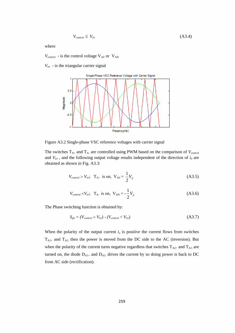
259
Vcontrol Vtri (A3.4)
where
Vcontrol - is the control voltage VA0 or VAN
Vtri - is the triangular carrier signal
Figure A3.2 Single-phase VSC reference voltages with carrier signal
The switches TA+ and TA- are controlled using PWM based on the comparison of Vcontrol
and Vtri , and the following output voltage results independent of the direction of i0 are
obtained as shown in Fig. A3.3:
Vcontrol Vtri; TA+ is on, VA0 = dV2
1 (A3.5)
Vcontrol Vtri; TA- is on, VAN = - dV2
1
(A3.6)
The Phase switching function is obtained by:
Sph = (Vcontrol Vtri) - (Vcontrol < Vtri) (A3.7)
When the polarity of the output current io is positive the current flows from switches
TA1+ and TA2- then the power is moved from the DC side to the AC (inversion). But
when the polarity of the current turns negative regardless that switches TA2+ and TA1- are
turned on, the diode DA1+ and DA2- drives the current by so doing power is back to DC
from AC side (rectification).

260
Figure A3.3 PWM output voltage of converter
In the same manner and for the other half cycle, when the polarity of the output current
io is positive the switches TA2+ and TA1- on, diode DA3+ and DA4- drives the current, then
the power is moved to the DC side from the AC (rectification). But when the polarity of
the current is negative, switches TA2+ and TA1- drives the current by so doing power is
back to AC from DC side (inversion). The comparison of Vcontrol with Vtri produces the
logic signals to control the switches in leg A and B:
vcontrol > vtriangle: TA1+ on and VAN = VDC
vcontrol < vtriangle: TA1- on and VAN = 0 (A3.8)
vcontrol > vtriangle: TA2+ on and VBN = VDC
vcontrol < vtriangle: TA2- on and VBN = 0 (A3.9)
In this method of PWM control the output voltage changes between zero and VDC or
zero and -VDC voltage levels as represented in Fig. 5.4. The voltage waveforms vAN and
vBN are displaced by 180o of the fundamental frequency with respect to each other. In
this regard, the harmonic components at the switching frequency in vAN and vBN are of
the same phase, given by :
o
BNAN 180 (A3.10)
The cancellation of the harmonic component at the switching frequency at the output
voltage waveform (v0 ) as shown in Fig. A3.4.
0 100 200 300 400 500 600-1
-0.5
0
0.5
1
One cycle
Sw
itchi
ng S
igna
l(t)[
p.u]
0 20 40 60 80 100 1200
0.5
1
1.5
2
Harmonics
Har
mon
ic M
agni
tude
Figure A3.4 Two-level phase output voltage waveform

261
The magnitude of the fundamental component of the output voltage between point A
and B can be determined by
DCAB
VV
.4 (A3.11)
The Phase switching function is obtained by:
Sph = (Vcontrol Vtri)-(Vcontrol<Vtri) (A3.12)
Therefore, the line switching functions are as shown in Fig. A3.7
Phase switching function
Sab = SFA1+ - SFA2+ ; Sbc = SFA2+ – SFA3+ ; Sca = SFA3+ – SFA1+ (A3.13)
50 100 150 200 250
-0.5
0
0.5
Phase Switching Function
50 100 150 200 250-1
-0.5
0
0.5
Magnitude
50 100 150 200 250-1
-0.5
0
0.5
Frequency(Hz)
Figure A3.8 Phase Switching Function PWM
Figure A3.7 Line Switching Function PWM

262
The load current block is used to obtain the load current (Ia, Ib, Ic). Assuming the load
consists of a balanced R-L load the load currents are derived as the ratio of the phase
voltage and respective impedance and is represented as shown in Fig. A3.9:
LjR
V
Z
VI AN
a
AN
a
(A3.14)
)120( o
a
BNBN
b tILjR
V
Zb
VI
(A3.15)
)120( o
a
CNCN
c tILjR
V
Zc
VI
(A3.16)
0 1 2 3 4 5 6 7-5
0
5Load Current
0 1 2 3 4 5 6 7-5
0
5
Magnitude
0 1 2 3 4 5 6 7-5
0
5
Frequency(Hz)
The switching current (ISFA1-, ISFA2-, ISFA3-) are determined by the product of the load
current with the corresponding switching function as shown in Fig. A3.10:
ISFA1- = Ia*<vtriangle, TA1- ; ISFA2- = Ib*<vtriangle, TA2- ; ISFA3- = Ic*<vtriangle, TA3
(A3.17)
0 1 2 3 4 5 6 70
0.5
1Switching Current PWM
0 1 2 3 4 5 6 70
0.5
1
Mag
nitud
e
0 1 2 3 4 5 6 70
0.5
1
Frequency(Hz)
The converter input current (Iin) can be obtained by
Iin = ISFA1- + ISFA2- + ISFA3- (A3.18)
Figure A3.9 Load Current (Ia, Ib, Ic)
Figure A3.10. Switching Current PWM

263
The converter phase current can be obtained by
iab = ISFA1- - ISFA2- ; ibc =ISFA1- - ISFA3- ; ica = ISFA3- - ISFA1- (A3.19)
0 100 200 300 400 500 600-1
-0.5
0
0.5
1
One cycle
Sw
itchin
g S
ignal(t)
[p.u
]
0 20 40 60 80 100 120
0
0.5
1
1.5
2
Harmonics
Harm
onic
Magnitude
One cycle
Sw
itchin
g S
ignal(t)
[p.u
]
0 100 200 300 400 500 600-1
-0.5
0
0.5
1
One cycle
Sw
itchin
g S
ignal(t)
[p.u
]
0 20 40 60 80 100 1200
0.5
1
1.5
2
Harmonics
Harm
onic
Magnitude
0 100 200 300 400 500 600-1
-0.5
0
0.5
1
One cycle
Sw
itchin
g S
ignal(t)
[p.u
]
0 20 40 60 80 100 120
0
0.5
1
1.5
2
Harmonics
Harm
onic
Magnitude
Figure A3.11 Twenty-one-level Phase Switching Function of a ten VSC Unipolar PWM
Converters Output voltage of phase a and phase b; (b) The amplitude of all harmonics for the output
voltage of phase a and phase b; (c) Output voltage of phase b and phase c; (d) The amplitude of all
harmonics for the output voltage of phase b and phase c; (e) Output voltage of phase c and phase a;
(f) The amplitude of all harmonics for the output voltage of phase c and phase a
a b
c d
e f

264
0 100 200 300 400 500 600-1.5
-1
-0.5
0
0.5
1
1.5
One cycle
Sw
itchin
g S
ignal(t)
[p.u
]
0 20 40 60 80 100 120
0
0.5
1
1.5
2
2.5
3
Harmonics
Harm
onic
Magnitude
0 100 200 300 400 500 600-2
-1
0
1
2
One cycle
Sw
itchin
g S
ignal(t)
[p.u
]
0 20 40 60 80 100 120
0
0.5
1
1.5
2
2.5
3
Harmonics
Harm
onic
Magnitude
0 100 200 300 400 500 600-1.5
-1
-0.5
0
0.5
1
1.5
2
One cycle
Sw
itchin
g S
ignal(t)
[p.u
]
0 20 40 60 80 100 120
0
0.5
1
1.5
2
2.5
3
Harmonics
Harm
onic
Magnitude
Figure A3.12. Twenty-one-level line-to-line Switching Function of a ten VSC Unipolar
PWM Converters Output voltage of phase a and phase b; (b) The amplitude of all harmonics
for the output voltage of phase a and phase b; (c) Output voltage of phase b and phase c; (d)
The amplitude of all harmonics for the output voltage of phase b and phase c; (e) Output
voltage of phase c and phase a; (f) The amplitude of all harmonics for the output voltage of
phase c
a b
c d
e f
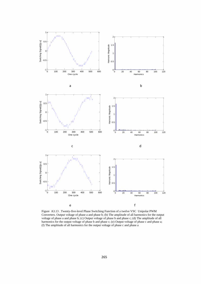
265
0 100 200 300 400 500 600-1
-0.5
0
0.5
1
One cycle
Sw
itchin
g S
ignal(t)
[p.u
]
0 20 40 60 80 100 120
0
0.5
1
1.5
2
Harmonics
Harm
onic
Magnitude
0 100 200 300 400 500 600-1
-0.5
0
0.5
1
One cycle
Sw
itchin
g S
ignal(t)
[p.u
]
0 20 40 60 80 100 120
0
0.5
1
1.5
2
Harmonics
Harm
onic
Magnitude
0 100 200 300 400 500 600-1
-0.5
0
0.5
1
One cycle
Sw
itchin
g S
ignal(t)
[p.u
]
0 20 40 60 80 100 120
0
0.5
1
1.5
2
Harmonics
Harm
onic
Magnitude
Figure A3.13 . Twenty-five-level Phase Switching Function of a twelve VSC Unipolar PWM
Converters. Output voltage of phase a and phase b; (b) The amplitude of all harmonics for the output
voltage of phase a and phase b; (c) Output voltage of phase b and phase c; (d) The amplitude of all
harmonics for the output voltage of phase b and phase c; (e) Output voltage of phase c and phase a;
(f) The amplitude of all harmonics for the output voltage of phase c and phase a
a b
c d
e f

266
0 100 200 300 400 500 600-1.5
-1
-0.5
0
0.5
1
1.5
One cycle
Sw
itchin
g S
ignal(t)
[p.u
]
0 20 40 60 80 100 120
0
0.5
1
1.5
2
2.5
3
Harmonics
Harm
onic
Magnitude
0 100 200 300 400 500 600-2
-1
0
1
2
One cycle
Sw
itchin
g S
ignal(t)
[p.u
]
0 20 40 60 80 100 120
0
0.5
1
1.5
2
2.5
3
Harmonics
Harm
onic
Magnitude
0 100 200 300 400 500 600-2
-1
0
1
2
One cycle
Sw
itchin
g S
ignal(t)
[p.u
]
0 20 40 60 80 100 120
0
0.5
1
1.5
2
2.5
3
Harmonics
Harm
onic
Magnitude
Figure A3.14. Twenty-five-level line-to-line Switching Function of a
twelve VSC Unipolar PWM Converters
Output voltage of phase a and phase b; (b) The amplitude of all harmonics
for the output voltage of phase a and phase b; (c) Output voltage of phase b
and phase c; (d) The amplitude of all harmonics for the output voltage of
phase b and phase c; (e) Output voltage of phase c and phase a; (f) The
amplitude of all harmonics for the output voltage of phase c
a b
c d
e f
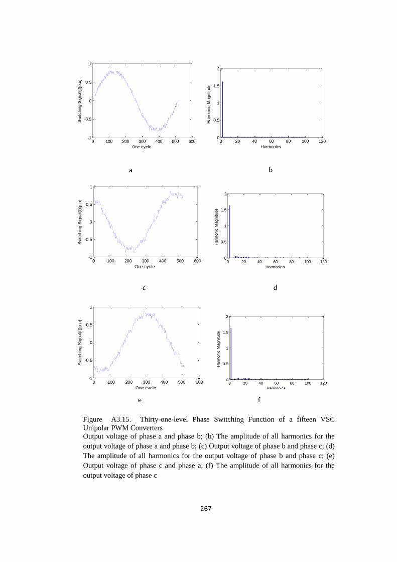
267
0 100 200 300 400 500 600-1
-0.5
0
0.5
1
One cycle
Sw
itchin
g S
ignal(t)
[p.u
]
0 20 40 60 80 100 1200
0.5
1
1.5
2
Harmonics
Harm
onic
Magnitude
0 100 200 300 400 500 600-1
-0.5
0
0.5
1
One cycle
Sw
itchin
g S
ignal(t)
[p.u
]
0 20 40 60 80 100 120
0
0.5
1
1.5
2
Harmonics
Harm
onic
Magnitude
0 100 200 300 400 500 600-1
-0.5
0
0.5
1
One cycle
Sw
itchin
g S
ignal(t)
[p.u
]
0 20 40 60 80 100 120
0
0.5
1
1.5
2
Harmonics
Harm
onic
Magnitude
Figure A3.15. Thirty-one-level Phase Switching Function of a fifteen VSC
Unipolar PWM Converters
Output voltage of phase a and phase b; (b) The amplitude of all harmonics for the
output voltage of phase a and phase b; (c) Output voltage of phase b and phase c; (d)
The amplitude of all harmonics for the output voltage of phase b and phase c; (e)
Output voltage of phase c and phase a; (f) The amplitude of all harmonics for the
output voltage of phase c
e f
a b
c d
e f

268
0 100 200 300 400 500 600-2
-1.5
-1
-0.5
0
0.5
1
1.5
2
One cycle
Sw
itchin
g S
ignal(t)
[p.u
]
0 20 40 60 80 100 120
0
0.5
1
1.5
2
2.5
3
Harmonics
Harm
onic
Magnitude
0 100 200 300 400 500 600-1.5
-1
-0.5
0
0.5
1
1.5
One cycle
Sw
itchin
g S
ignal(t)
[p.u
]
0 20 40 60 80 100 120
0
0.5
1
1.5
2
2.5
3
Harmonics
Harm
onic
Magnitude
0 100 200 300 400 500 600-2
-1
0
1
2
One cycle
Sw
itchin
g S
ignal(t)
[p.u
]
0 20 40 60 80 100 1200
0.5
1
1.5
2
2.5
3
Harmonics
Harm
onic
Magnitude
The waveforms and harmonic spectraof the phase and line-to-line voltages for three-
phase 12-level and 15-level respectively. From the figures, it can be seen that the usual
stairs structure of the MMC is defined and heading to total sinusoidal waveforms, hence
leading to cancellation of all the harmonic contents. Also, the harmonic spectra do not
Figure A3.16. Thirty-one-level line-to-line Switching Function of a
fifteen VSC Unipolar PWM Converters. Output voltage of phase a and
phase b; (b) The amplitude of all harmonics for the output voltage of phase
a and phase b; (c) Output voltage of phase b and phase c; (d) The
amplitude of all harmonics for the output voltage of phase b and phase c;
(e) Output voltage of phase c and phase a; (f) The amplitude of all
harmonics for the output voltage of phase c
a b
c d
e f

269
indicate any highly significant harmonic due to the common mode cancellation between
the converter phase legs. Instead, only the occurrence of the first significant harmonic is
found which has no significant threat in the network.

270
Appendix A4
A4.1. Induction Generator abc model
The Fig. A4.1 shows induction generator with rotor and stator windings neglecting
saturation and losses in the core.
The voltages applied to each stator and rotor phases is given as
[V] = [vA vB vC va vb vc]T (A4.1)
Similarly, the currents in each stator and rotor phases is given as
[I] = [IA IB IC ia ib ic]T (A4.2)
Also, the fluxes linked with each stator and rotor phases is obtained as
[ ] = [ A B C a b c ]T (A4.3)
Figure A4.1. Six-pole induction generator with rotor and stator windings
The voltage V matrix is given as
dt
dIRV
(A4.4)
where
[R] is the resistance matrix
IL (A4.5)
IC
vC
vc
ic
rc vB
IB
rb
ib
vb
va
ia
r
r
SC
SB
vA
IA
SA
ra
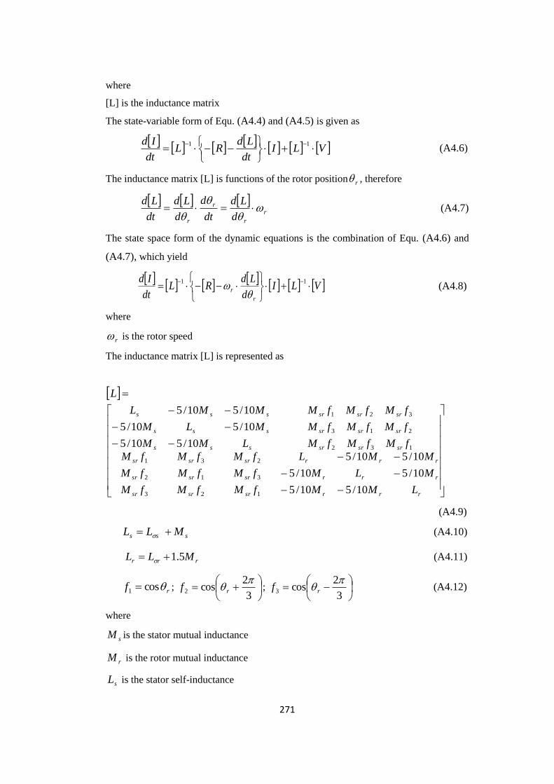
271
where
[L] is the inductance matrix
The state-variable form of Equ. (A4.4) and (A4.5) is given as
VLIdt
LdRL
dt
Id
11
(A4.6)
The inductance matrix [L] is functions of the rotor position r , therefore
r
r
r
r d
Ld
dt
d
d
Ld
dt
Ld
(A4.7)
The state space form of the dynamic equations is the combination of Equ. (A4.6) and
(A4.7), which yield
VLId
LdRL
dt
Id
r
r
11
(A4.8)
where
r is the rotor speed
The inductance matrix [L] is represented as
L
r
r
r
r
r
r
r
r
r
sr
sr
sr
sr
sr
sr
sr
sr
sr
srsrsrsss
srsrsrsss
srsrsrsss
L
M
M
M
L
M
M
M
L
fM
fM
fM
fM
fM
fM
fM
fM
fM
fMfMfMLMM
fMfMfMMLM
fMfMfMMML
10/5
10/5
10/5
10/5
10/5
10/5
10/510/5
10/510/5
10/510/5
1
3
2
2
1
3
3
2
1
132
213
321
(A4.9)
sss MLL (A4.10)
rrr MLL 5.1 (A4.11)
rf cos1 ;
3
2cos2
rf ;
3
2cos3
rf (A4.12)
where
sM is the stator mutual inductance
rM is the rotor mutual inductance
sL is the stator self-inductance
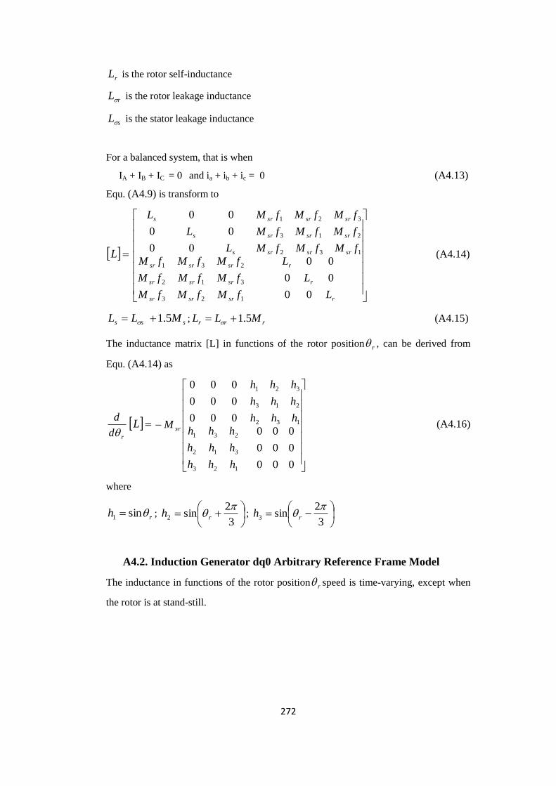
272
rL is the rotor self-inductance
rL is the rotor leakage inductance
sL is the stator leakage inductance
For a balanced system, that is when
IA + IB + IC = 0 and ia + ib + ic = 0 (A4.13)
Equ. (A4.9) is transform to
L
r
r
r
sr
sr
sr
sr
sr
sr
sr
sr
sr
srsrsrs
srsrsrs
srsrsrs
L
L
L
fM
fM
fM
fM
fM
fM
fM
fM
fM
fMfMfML
fMfMfML
fMfMfML
0
0
0
0
0
0
00
00
00
1
3
2
2
1
3
3
2
1
132
213
321
(A4.14)
sss MLL 5.1 ; rrr MLL 5.1 (A4.15)
The inductance matrix [L] in functions of the rotor position r , can be derived from
Equ. (A4.14) as
rd
d
L
0
0
0
0
0
0
0
0
0
000
000
000
1
3
2
2
1
3
3
2
1
132
213
321
h
h
h
h
h
h
h
h
h
hhh
hhh
hhh
M sr (A4.16)
where
rh sin1 ;
3
2sin2
rh ;
3
2sin3
rh
A4.2. Induction Generator dq0 Arbitrary Reference Frame Model
The inductance in functions of the rotor position r speed is time-varying, except when
the rotor is at stand-still.

273
Figure. A4.2. Induction generator dq0 arbitrary reference frame model
The transformation of Equ. (A4.4) yield Equ. (A4.17), which is the voltage in arbitrary
reference frame model.
0
0
r
rq
rd
s
qs
ds
v
v
v
v
v
v
=
0
00
0
0
0
0
0
0
0
0
0
0
0
0
0
0
00000
0000
0000
0
0
0
0
0
0
0
0
0
0
0
0
0
0
0
0
000000
00000
00000
0
0
0
0
0
0
0
0
0
0
0
0
0
00000
0000
0000
0
0
0
0
0
0
0
0
0
0
0
0
0
0
0
00000
00000
00000
r
rq
rd
s
sq
sd
r
r
r
m
m
s
ms
ms
rgs
rgs
gs
gs
r
r
r
m
m
S
ms
ms
r
rq
rd
s
sq
sd
i
i
i
i
i
i
L
L
L
L
L
L
LL
LL
L
L
L
L
L
L
LL
LL
dt
d
R
R
R
R
R
R
(A4.17)
In more compact form Equ. (A4.17) can be represented as
q-axis 0s
0-axis
0r qs
qr
d-axis
Phase-a Stator-axis
Phase-a
Rotor-axis

274
ILLdt
dRV
(A4.18)
The linkage fluxes and currents are related as
IL (A4.19)
where
srm ML2
3 is the mutual inductance in the general reference frame
mss LLL is the stator self inductance
mrr LLL is the rotor self inductance
A4.3. Induction Generator model in Steady State
An equivalent electrical circuit of induction generator is as shown in Fig. A4.3, where rs
= stator resistance, '
rr = rotor resistance, sx = stator leakage reactance, '
rx = rotor
leakage reactance, mr iron loss resistance, mx = magnetizing reactance,
Figure A4.3. Equivalent circuit of induction generator
From Equ. (A4.17) in the rotating reference frame rgs
The steady-state voltage formulations are obtain as
rmmsss IjXrIjXrsV //
rmmrrr IjsXrIjsXrrV //
(A4.20)
Equ. (A4.20)can be represented in matrix form as follow
mx
0I
'1rr
s
s
'
rx '
rr sx sr
~
2I mr
~
E
~
1I ~
sV

275
r
s
rrrm
mmss
I
I
jsXrjsXr
jXrjXr
r
s
V
V//
// (A4.21)
In more compact form Equ. (A4.21)can be represented as
IZV (A4.22)
where
sX is the self reactance of the stator windings
rX is the self reactance of the rotor windings
The stator and rotor currents are obtained as
VZI 1
(A4.23)
The active power Ps of the stator is obtained as
SSs IValP Re2
3 (A4.24)
The reactive power Qs of the stator is obtained as
SSs IVagQ Im2
3 (A4.25)
Similarly, the active power Pr of the rotor is obtained as
rrr IValP Re2
3 (A4.26)
The reactive power Qr of the rotor is obtained as
rrr IVagQ Im2
3 (A4.27)
In the equivalent circuit Fig. A4.3, the power loss in sr and mr represents the primary
copper loss and the core loss. The power loss in the resistance '1
rrs
s must therefore
represent the average input of power to the rotor, for there can be no dissipation of
power in the reactance mx and'
rx . Thus the input of power per phase to the rotor
is s
rI r
'2'
2 , but the power dissipated in the actual resistance of the rotor circuit is
only '2'
2 rrI .

276
Therefore, generator input power is rrs
sI
12'
2.
If P is the total power absorbed by the rotor, then
Electromagnetic power input to rotor is
s
rInP r
'2'
2 (A4.28)
The power loss in rotor resistance is
'2'
2 rrInsP (A4.29)
Mechanical power output is
'2'
2
11 rr
s
sInPs
(A4.30)
where n is the number of phases
The torque T exerted on the rotor by the rotating magnetic field. If there are P pairs of
poles, the angular velocity of the field isP
S
, and the rotating field therefore does
work at rate .Ts This would obviously be true if the rotating field were produced by
physical poles on the stator, driven mechanically at a speed ,s the electromagnetic
field is the same when a poly-phase winding produces the rotating field, so the work
done must be the same. Since the rotor runs at a speed sp s 1 ,
then mechanical power output given is as
TsT sr 1 (A4.31)
The difference between the work done by the field and the mechanical output must be
absorbed in rotor losses, that is
TsT srs (A4.32)
Thus,
Electromechanical power input to rotor
P = Ts (A4.33)
Power loss in rotor resistance
TsTP srs (A4.34)
Mechanical power output
TsTP sr 1 (A4.35)
The fraction of the input power lost in rotor resistance is equal to the fractional slip s,
since there must always be some slip between the rotor and the rotating magnetic field,

277
this present an unavoidable power loss. The ratio of mechanical power output to
electromagnetic power input is known as the rotor efficiency, and is equal to s1 .
The torque may be determined for a given value of slip by equating expressions (A4.28)
and (A4.33) for electromagnetic power, and obtaining the value of '
2I from the
equivalent circuit of Fig. A4.3..
For a machine with n phases and P pole pairs, the torque is
2
'
22
2
1
'
2
s
rX
V
s
rnPT
(A4.36)
Alternatively,
sX
r
r
sXX
VnPT
'
2
'
2
2
1 1
(A4.37)
A4.4. Motoring and Generating Regions of Induction Machine
Since the slip s is related to the rotor speed r by s
rss
and equ. (A4.37) gives
the torque /speed relationship for the induction machine. Fig. A4.4a and Fig. A4.4b
shows a typical torque/slip characteristic.
The slip of induction generator at harmonic frequency is given as
s
rs
hh
hhS
(A4.38)
The synchronous speed is
p
s
(A4.39)
where
Sh = slip for hth harmonics, r = rotor speed, s = synchronous speed, = f2 , p =
number of poles.
It is noted that s < r , the slip is always negative as it should be for generator action.

278
-1 -0.5 0 0.5 1-15
-10
-5
0
5
10
15
slip
Torq
ue (
pu)
Motoring
Region
Generating
Region
-1 -0.5 0 0.5 1
-15
-10
-5
0
5
10
slip
Torq
ue(p
u)
Generator
Region
Motoring
Region
(a) (b)
Figure A4.4. (a) Typical torque-slip characteristic of an induction machine (b) Torque-
slip curves with increased rotor resistance
It should be noted here that there can be no induced rotor currents when s = 0 and
sr , so the torque must be zero at this point. There are two distinct regions to the
torque/slip characteristic shown in Fig. A4.4a and Fig. A4.4b which is generating region
and motoring region.
A4.4.1. Motoring region
In the motoring region as shown in Fig. A4.4, the rotor speed r is positive but less
than the synchronous speed s , the torque is also positive; in addition the machine
converts electrical power into mechanical power. The slip varies from 1 when the rotor
is on standstill to 0 when the rotor runs at the synchronous speed. The resistance
'
2
1r
s
s is positive and greater than
'
2r , thus the total electrical power absorbed by the
rotor exceeds the power dissipated in the rotor resistance, and the balance is extracted as
mechanical power at the shaft. The overall efficiency of the machine cannot exceed the
rotor efficiency of 1 – s, induction motors operate with a small value of slip. The full-
load slip can be as low as 1 per cent in large machines and can exceed 5 per cent in
small machine; therefore the normal rotor speed is always close to the synchronous
speed [37].
A4.4.2. Generating region
In the event that the rotor is driven mechanically so that its speed exceeds the
synchronous speed, the torque reverses and the machine absorbs mechanical power.

279
Both the slip and '
2
1r
s
s are negative in this region, the rotor therefore transmits
electrical power to the stator, and the induction machine exhibit generator characteristic
as shown Fig. A4.4.
An induction machine requires an external source of reactive power for it to act as a
generator, since the magnetising current flowing in mX cannot be provided by the
rotor. While the synchronous machine provides its own magnetising current because of
the field winding on the rotor, there is no need for external source. An AC grid fed
induction generator will require reactive power for its operation, but can also operate
without an external AC grid by connecting a capacitor bank to the stator terminals
which will supply the required reactive power and the machine will self-excite.
As a result, induction generators have gained an advantage in industrial plants and as
well as wind turbine feeding oil and gas platforms, because they are more robust and
light in weight than synchronous generators.
The presence of negative resistance (i.e., when slip is negative), implies that during the
generating mode, power flows from the rotor to the stator in the induction generator.
An induction generator needs AC excitation current for its running. The machine is
either self excited or externally excited. The steady-state per-phase equivalent circuit of
a self-excited induction generator is as shown in the Fig. A4.4.
A4.4.3. Asynchronous motor
It is evident that single cage induction motor model as shown in Fig. A4.5 is not able to
capture both the starting characteristics and the breakdown torque characteristics of a
cage induction motor. Therefore, for motor start-up simulations the double cage model
is recommended and is as represented in Fig. 6. A4.6. The induction motor has
remained the most popular type of motor for industry applications. The primary
advantage of the induction motor is its straightforward rotor construction leading to
low-cost, ruggedness, and low-maintenance requirement.

280
Figure A4.5. Per-phase single-cage equivalent circuit of an induction motor
Figure A4.6. Per-phase double-cage equivalent circuit of an induction motor
The equivalent circuit for the double cage model is shown in Fig. A4.6, the impedances
as admittances are obtained in harmonic domain as follows:
1 SSS jhXRY (A4.40)
1
11
mC
mjhXR
Y (A4.41)
1
11
1
jhX
s
RY R
R (A4.42)
1
22
2
jhX
s
RY R
R (A4.43)
Total admittance is
sjhXR
s
sjhXR
s
jhXR
RjhX
jhXRY
RRmC
cm
SS 2211
1
(A4.44)
Applying Kirchoff’s law at node V2:
21221 RRmS YYYVYVV (A4.45)
2121 RRmSS YYYYVYV (A4.46)
Im
I
I2
jhXm RR/s
jhXR jhXS
I1
RS
RC
V1
+
-
+
Vm
-
j hXS V2 I3 I2
RR2/s RR1/s jhXm
Im
I
RC
I1 jhXR2 jhXR1
RS
+
V1
-
+
Vm
-
V3

281
21
1
2
RRmS
S
YYYY
YVV
(A4.47)
The stator current Is is given as
Ss YVVI 21 (A4.48)
While the rotor current IR1 and IR2 are obtain as:
121 RR YVI (A4.49)
222 RR YVI
The torque developed in the motor (N-m) is:
2
222
11
RR
RR I
s
RI
s
RT (A4.50)
Induction motor Data
r1 = 0.220; % Stator resistance
x1 = 0.430; % Stator reactance
r2 = 0.127; % Rotor resistance
x2 = 0.430; % Rotor reactance
xm = 15.0; % Magnetization branch reactance
v_phase = 208 / sqrt(3); % Phase voltage
n_sync = 1800; % Synchronous speed (r/min)
w_sync = 188.5; % Synchronous speed (rad/s)
0 500 1000 1500 20000
200
400
600
800
1000
Mechanical Speed
in
d
\t_ind1 = 1%
\t_ind2 = 20%
\t_ind3 = 40%
\t_ind4 = 60%
\t_ind5 = 80%
\t_ind6 = 10%
0 0.2 0.4 0.6 0.8 10
200
400
600
800
1000
Slip
in
d
(a) (b)

282
0 50 100 150 2000
5
10
15
20
Mechanical speed (rad/s)
PO
UT (
kW
)
0 0.2 0.4 0.6 0.8 10
5
10
15
20
Slip
PO
UT (
kW
)
900 920 940 960 980 1000
-50
0
50
100
150
200
nm
(r/min)
(
%)
power converter
output power
motor efficiency
Figure A4.7. Induction motor: (a) Motor Torque versus Speed Characteristic (b) Motor
torque versus slip (c) output power versus Speed (d) output power versus slip (e) output
power and efficiency
Harmonic model of transformers
The physical model of a single-phase transformer is as shown in Fig. A4.8.
The corresponding electrical and magnetic equations are
Figure A4.8. Physical model of a single-phase transformer
(c) (d)
(e)
ip(t) is(t)
m
Ns Np
p s
_
+ +
Vp(t) Vs(t)
-
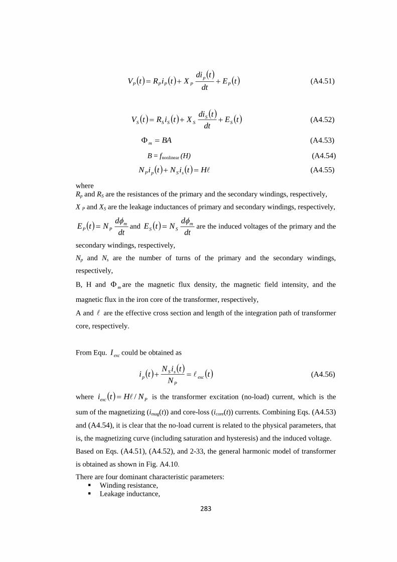
283
tEdt
tdiXtiRtV P
p
PPPP (A4.51)
tEdt
tdiXtiRtV S
S
SSSS (A4.52)
BAm (A4.53)
B = fnonlinear (H) (A4.54)
HtiNtiN sSpP (A4.55)
where
Rp and RS are the resistances of the primary and the secondary windings, respectively,
X P and XS are the leakage inductances of primary and secondary windings, respectively,
dt
dNtE m
PP
and
dt
dNtE m
SS
are the induced voltages of the primary and the
secondary windings, respectively,
Np and Ns are the number of turns of the primary and the secondary windings,
respectively,
B, H and m are the magnetic flux density, the magnetic field intensity, and the
magnetic flux in the iron core of the transformer, respectively,
A and are the effective cross section and length of the integration path of transformer
core, respectively.
From Equ. excI could be obtained as
tN
tiNti exc
P
sS
p (A4.56)
where Pexc NHti / is the transformer excitation (no-load) current, which is the
sum of the magnetizing (imag(t)) and core-loss (icore(t)) currents. Combining Eqs. (A4.53)
and (A4.54), it is clear that the no-load current is related to the physical parameters, that
is, the magnetizing curve (including saturation and hysteresis) and the induced voltage.
Based on Eqs. (A4.51), (A4.52), and 2-33, the general harmonic model of transformer
is obtained as shown in Fig. A4.10.
There are four dominant characteristic parameters:
Winding resistance,
Leakage inductance,

284
Magnetizing current, and
Core-Loss current
Some models assume constant values for the primary and the secondary resistances.
However, most references take into account the influence of skin effects and proximity
effects in the harmonic model. Since primary ( p ) and secondary ( s ) leakage
fluxes mainly flow across air, the primary and the secondary leakage inductances can be
assumed to be constants. The main difficulty arises in the computation of the
magnetizing and core-loss currents, which are the main sources of harmonics in power
transformers.
Figure A4.9. Equivalent circuit linear single-phase, steady state transformer model
The total admittance of the transformer is:
SSmC
Cm
PP
TRANShXjRhXjR
RhXj
hXjRY
11 (A4.57)
Figure A4.10. General harmonic model of a transformer
Rs
mXjh
magI~
si~
shXj phXj
RP pi~
~
coreI
~
exeI
+
-
~
pV RC
+
~
pE
-
+
~
sV
_
P2 P1

285
When considering the addition of a large non-linear load to an oil and gas power
system, it may be warranted to perform harmonic modelling analysis of the system if it
comprises 25% or more of the plant load. Harmonic modelling is a mathematical way of
predicting harmonic distortion levels and potential resonances based on available power
network data. All but the simplest of systems will require computer software such as
MATLAB/SIMULINK to perform this analysis. Components such as transformers,
capacitors, motors, and the utility system impedance are taken into account, and non-
linear loads are represented by multiple frequency harmonic current sources. Such a
modelling study will indicate if harmonic levels will fall within limits.
286
Appendix A5
A5.1. AC-DC Converter
AC-DC converters (rectifiers) are classified into two main categories i.e. controlled and
uncontrolled rectifiers. In an uncontrolled rectifier, the dc output is constant if the ac
input voltage is constant. These converters are classified according to their input supply
and the way the diodes are connected. They are half wave, full wave bridge type and
full wave centre tapped transformer type [1-5]. DC obtained from this rectifier is further
converted into desired amplitude and frequency.
PWM rectifiers have replaced the conventional three phase controlled rectifier (PCR) due
to their high efficiency, good voltage regulation, nearly unity power factor and small
input/output filter size depending upon switching frequency. PWM rectifiers are
normally operated at high switching frequency where low frequency harmonics are
easily suppressed. PWM rectifiers are becoming more popular due to the availability of
fast switching, high voltage and high current IGBT’s [6-8].
A three-phase PWM regenerative boost rectifier [9] is shown in figure 5.5a. The output
voltage is greater than the peak of the line to line RMS voltage in this rectifier. This is a
four quadrant rectifier capable of bidirectional power flow. Operation of this rectifier is
similar to a High Voltage Switch Mode Power Supply (HV-SMPS) boost converter.
When DA1+ is turned on, voltage is applied across the inductor and it gets energized.
When DA2+ is turned off, inductor de-energizes through the diode of DA1+ charging the
capacitor. Unity power factor is achieved by controlling the current in the inductor.
Multi-level ac-dc converters can also be used to develop modular multi-level converter
(MMC) as depicted in Fig.5.11. This device can act as a node device in multi-terminal
network, where the first node acts as rectifier and the node directly connected to it acts
as an inverter as depicted in Fig. 7.1. The preferred ac-dc converter topology is suitable
for high-power applications; operates at constant frequency under a PWM strategy. The
sub-module full-bridge of the modular multi-level converter consists of a DC input
voltage source vi and a six controllable switching sequence as shown in Table 7.1.
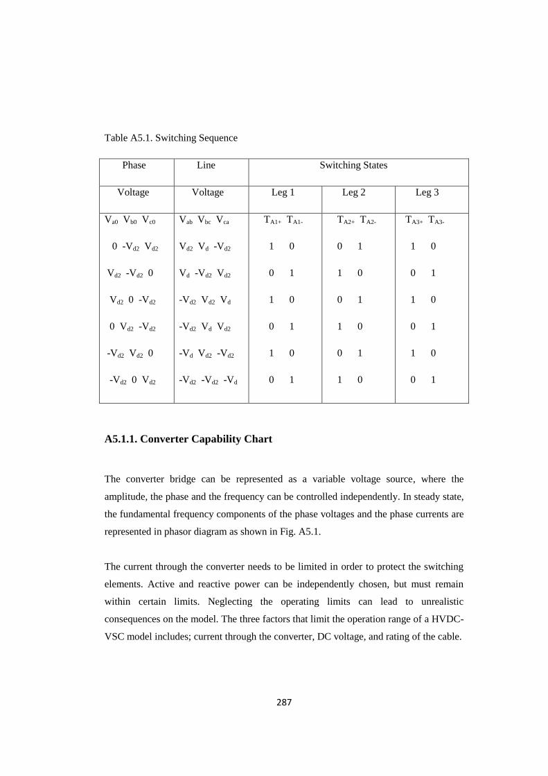
287
Table A5.1. Switching Sequence
Phase Line Switching States
Voltage Voltage Leg 1 Leg 2 Leg 3
Va0 Vb0 Vc0
0 -Vd2 Vd2
Vd2 -Vd2 0
Vd2 0 -Vd2
0 Vd2 -Vd2
-Vd2 Vd2 0
-Vd2 0 Vd2
Vab Vbc Vca
Vd2 Vd -Vd2
Vd -Vd2 Vd2
-Vd2 Vd2 Vd
-Vd2 Vd Vd2
-Vd Vd2 -Vd2
-Vd2 -Vd2 -Vd
TA1+ TA1-
1 0
0 1
1 0
0 1
1 0
0 1
TA2+ TA2-
0 1
1 0
0 1
1 0
0 1
1 0
TA3+ TA3-
1 0
0 1
1 0
0 1
1 0
0 1
A5.1.1. Converter Capability Chart
The converter bridge can be represented as a variable voltage source, where the
amplitude, the phase and the frequency can be controlled independently. In steady state,
the fundamental frequency components of the phase voltages and the phase currents are
represented in phasor diagram as shown in Fig. A5.1.
The current through the converter needs to be limited in order to protect the switching
elements. Active and reactive power can be independently chosen, but must remain
within certain limits. Neglecting the operating limits can lead to unrealistic
consequences on the model. The three factors that limit the operation range of a HVDC-
VSC model includes; current through the converter, DC voltage, and rating of the cable.
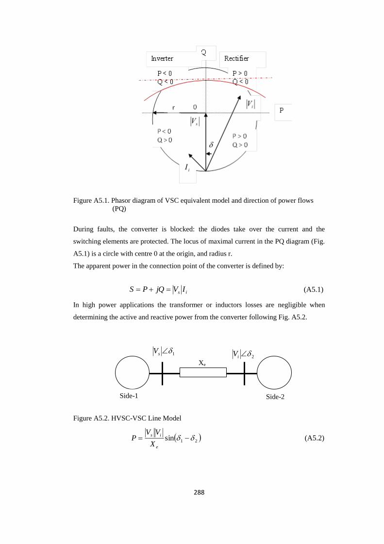
288
Figure A5.1. Phasor diagram of VSC equivalent model and direction of power flows
(PQ)
During faults, the converter is blocked: the diodes take over the current and the
switching elements are protected. The locus of maximal current in the PQ diagram (Fig.
A5.1) is a circle with centre 0 at the origin, and radius r.
The apparent power in the connection point of the converter is defined by:
is IVjQPS (A5.1)
In high power applications the transformer or inductors losses are negligible when
determining the active and reactive power from the converter following Fig. A5.2.
Figure A5.2. HVSC-VSC Line Model
21sin e
is
X
VVP (A5.2)
2iV Xe
1sV
Side-1 Side-2

289
21
2
cos e
si
e
i
X
VV
X
VQ (A5.3)
where eX is the equivalent reactance of the coupling transformer
Real power flow:
• δ1> δ2 =>P12 is +ve: Real power flows from Side-1 to Side-2
• δ1< δ2 =>P12 is -ve: Real power flows from Side -2 to Side -1
Reactive power flow:
• |V1| > |V2|: Reactive power flows from Side -1 to Side -2
• |V1| < |V2|: Reactive power flows from Side -2 to Side -1
It can be deduced from (A5.2) and (A5.3) that the VSC neither injects nor absorbs
active and reactive power from the system when iV - sV = 0, this follows that is =
0.
Also, the VSC inject reactive power when iV > sV and absorb reactive power when
iV < sV .
As shown in Fig. A5.2 the voltage drop V over the reactor vX can be described as:
qp VjVV (A5.4)
i
vv
i
vv
V
QRPXj
V
QXPR
(A5.5)
If qV << pi VV
then i
vv
V
QXPRV
For AC networks most power circuit satisfy vX >> vR , therefore the voltage drop V
Knowing that depends only on the reactive power flow Q.
sin2 is + cos
2 is = 1 (A5.6)
Therefore, sin is and cos is could be eliminated, hence
222
cs
e
e
s
cs
e
VV
X
X
VQ
VV
PX= 1 (A5.7)
and
22
2
2
e
s
e
cs
X
VQP
X
VV (A5.8)
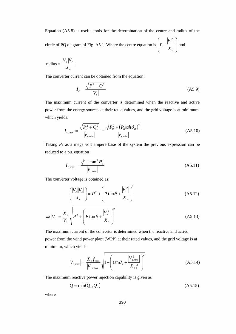
290
Equation (A5.8) is useful tools for the determination of the centre and radius of the
circle of PQ diagram of Fig. A5.1. Where the centre equation is
e
s
X
V 2
,0 and
radius = e
cs
X
VV.
The converter current can be obtained from the equation:
s
cV
QPI
22 (A5.9)
The maximum current of the converter is determined when the reactive and active
power from the energy sources at their rated values, and the grid voltage is at minimum,
which yields:
min,
22
max,
s
RR
cV
QPI
=
min,
22
s
RRR
V
tahPP (A5.10)
Taking PR as a mega volt ampere base of the system the previous expression can be
reduced to a pu. equation
min,
2
max,
tan1
s
s
cV
I
(A5.11)
The converter voltage is obtained as:
22
2 tan
e
s
e
sc
X
VPP
X
VV (A5.12)
22
2 tan
e
s
s
e
cX
VPP
V
XV (A5.13)
The maximum current of the converter is determined when the reactive and active
power from the wind power plant (WPP) at their rated values, and the grid voltage is at
minimum, which yields:
22
max,
max,
max
max, tan1
fX
V
V
fXV
e
s
s
s
e
c (A5.14)
The maximum reactive power injection capability is given as
vc QQQ ,min (A5.15)
where

291
22
max, PIVQ csc - the converter-current-rating
e
s
e
sc
vX
VP
X
VVQ
2
2
2
max,
- the converter-voltage-rating limits
A5.2. Operation Modes
The operating modes which can be adopted in AC and DC sides of each station are
examined.
A5.2.1. AC side Operating Modes
VSC on its AC side can either control the reactive power or AC voltage at the point of
the common connection (PCC) as depicts in Fig. 7.4.
(a)
Active and reactive power control mode
(b)
Active and AC voltage control mode
Figure A5.3: (a) PQ bus connected to VSC converter.(b) PV bus connected to VSC
converter.
If in an N multi-terminal HVDC-VSC, the reference power of all converters at the PCC
is known, every PCC from AC system’s point of view can be seen as either a PV or PQ
bus depending on the control mode of converter connected to that bus as shown in
AC Source
PDC
QCONV Xeq
PCONV PCC
VSC
Vset
PDC
Xeq
PCONV PCC
AC Source VSC

292
Figure A5.3. Therefore all N converters excluding the slack converter can be separately
modelled at each AC bus.
A5.2.2. DC side Operating Modes
In a two terminal VSC-HVDC, at least one of the two converters must have dc voltage
regulation mechanism for normal operation of a point-to-point VSC-HVDC connection.
Similarly, in a multi-terminal VSC-HVDC configuration there must be dc voltage
regulation for normal operation of the system. As described in the previous chapter
there are two options for dc voltage control of a single VSC station; namely: constant dc
voltage control and dc voltage droop control. It was also mentioned in section 2.5 that
stable operation cannot be achieved if both converters of the two-terminal VSC-HVDC
are assigned to constant dc voltage control mode.
The same condition applies to multi-terminal VSC-HVDC, i.e. there must not be more
than one converter station in the dc grid assigned to constant dc voltage control mode.
(If there are two converters with constant dc voltage control, there will be a hunting
phenomena, analogous to frequency hunting in ac grids in the presence of multiple
synchronous generators with fixed frequency control). Taking the constraints mentioned
above, we get three possible control modes of MTDC; namely: master-slave control, dc
voltage droop control and master-slave with dc droop. Each of these is explained below.
A5.2.3. PQ Bus/Load Bus
A pure load bus is a PQ bus. A load bus has no generating facility, that is,
PG1 = QG1 = 0.
At this type of bus, the net real power Pi and the reactive power Qi are known as
Pi = PG1 – PD1 and Qi = QG1 – QD1 (A5.16)
Pi known ( PDi known, PGi zero)
Qi known ( QDi known, QGi zero) ~
iV unknown – this is voltage magnitude
i unknown – this is voltage angle
where

293
PG1, QG1 are the real and reactive power generations at the bus respectively
PD1, QD1 are the real and reactive power demands at the bus respectively
PG1 and QG1 are specified and PD1 and QD1 are known from forecasting
A5.2.4. PV Bus/Generator Bus
A generator whether wind or gas turbine are always connected to a PV bus. Therefore
the net power Pi, known as PDi is known from forecasting
Pi known
Qi unknown
Pi known ( PGi specified, PDi known) ~
iV known (specified)
Qi unknown (QDi unknown, QGi known)
i unknown
A5.2.5. Slack Bus/Swing Bus/Reference Bus, Generator with Larg Capacity
In this bus, normally voltage magnitude is set to 1 pu and voltage angle is set to zero.
The real and reactive powers are not specified.
~
1V known (specified)
1 known (specified, typically 01 reference)
P1 unknown (PD1 known, PG1 unknown)
Q1 unknown (QD1 known, QG1 unknown)
Real and reactive powers cannot be fixed prior at all the buses, since the net complex
power flow into the network is not known beforehand. Therefore, the power losses are
unspecified until the load flow study is ended. This follows that it is imperative to have
one bus at which complex powers is unspecified as to supply the difference in the total
system load with losses. Also, the sum of the complex powers known at the other buses.
This type of bus is named swing bus and irrevocable termed generator bus. On the event
that the swing bus is not known, then the bus connected to the largest generating station
is usually chosen as the reference bus. It should be reiterated here that wind farm (wind
turbine) bus should not be named slack bus, due to its variable voltages as a result of
wind speed variation.
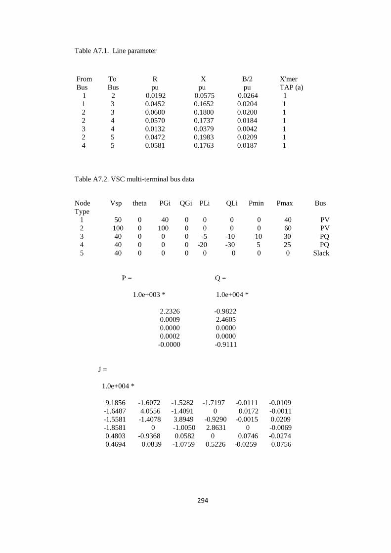
294
Table A7.1. Line parameter
From To R X B/2 X'mer
Bus Bus pu pu pu TAP (a)
1 2 0.0192 0.0575 0.0264 1
1 3 0.0452 0.1652 0.0204 1
2 3 0.0600 0.1800 0.0200 1
2 4 0.0570 0.1737 0.0184 1
3 4 0.0132 0.0379 0.0042 1
2 5 0.0472 0.1983 0.0209 1
4 5 0.0581 0.1763 0.0187 1
Table A7.2. VSC multi-terminal bus data
Node Vsp theta PGi QGi PLi QLi Pmin Pmax Bus
Type
1 50 0 40 0 0 0 0 40 PV
2 100 0 100 0 0 0 0 60 PV
3 40 0 0 0 -5 -10 10 30 PQ
4 40 0 0 0 -20 -30 5 25 PQ
5 40 0 0 0 0 0 0 0 Slack
P = Q =
1.0e+003 * 1.0e+004 *
2.2326 -0.9822
0.0009 2.4605
0.0000 0.0000
0.0002 0.0000
-0.0000 -0.9111
J =
1.0e+004 *
9.1856 -1.6072 -1.5282 -1.7197 -0.0111 -0.0109
-1.6487 4.0556 -1.4091 0 0.0172 -0.0011
-1.5581 -1.4078 3.8949 -0.9290 -0.0015 0.0209
-1.8581 0 -1.0050 2.8631 0 -0.0069
0.4803 -0.9368 0.0582 0 0.0746 -0.0274
0.4694 0.0839 -1.0759 0.5226 -0.0259 0.0756

295
Bus kV Angle
No pu Degree
1 50.0000 0.0000
2 99.9600 -32.2111
3 74.4223 -25.1607
4 71.8498 -28.7345
5 40.0600 -19.9862


