
Growth Codes:Maximizing Sensor Network Data
Persistence
Abhinav Kamra, Vishal Misra, Dan RubensteinDepartment of Computer Science, Columbia
UniversityJon FeldmanGoogle Labs
ACM SIGCOMM 2006

Outline
Problem Description Solution Approach: Growth Codes Experiments and Simulations Conclusions

Background: A generic sensor network
Sink(s)
Sensor Nodes Data follows
multi-hop path to sink(s)
Sensed Data
x1 x9
x10
x12 x11
x13
x4
x5
x6
x3
x2
x8
x7
A few node failures can break the data flow
Generic Aim: Collect data from all nodes at sink(s)

Data Persistence
We define data persistence of a sensor
network to be the fraction of data generated within the network that eventually reaches the sink.
Focus of Work: Maximizing Data Persistence

Specific Context: Disaster Scenarios
e.g., Monitoring earthquakes, fires, floods, war zones
Problems in this setting Congestion near sink(s)
All nodes simultaneously forward data Overwhelm sink(s) capacity
Congestion near sinkVirtual queue:

Specific Context: Disaster Scenarios - 2
Problems in this setting Network Collapsing: nodes failing rapidly
Pre-computed routes may fail Data from failed nodes can be lost Data Recovery from subset of nodes
acceptable

Challenges Networking Challenges:
Disaster scenarios: feedback often infeasible Frequent disruptions to routing tree if setup Difficult to predict node failures: sink locations
unknown, surviving routes unknown Difficult to synchronize nodes’ clocks
Coding Challenges: Data source distributed (among all sensor
nodes) Prior approaches (Turbo codes, LDPC codes) aim at
fast complete recovery Sensor nodes have very limited memory,
CPU, bandwidth

Maximize Data Persistence
Preserve data from failed sensor nodes
Deliver data to sink(s) as fast as possible
Objectives
6 of 10 symbols reach sink. Persistence = 60%
Fraction of data that eventually reaches the sink(s)
x1
x9
x5
x3
x2x8
x10
x12
x11
x6
+
=
Sink
Data Persistence

Limitations of Previous Work
Channel Coding based(e.g. Turbo Codes [Anderson-ISIT94], LT Codes [Luby02])
Aim for complete recovery in minimum time Difficult to implement with distributed
sources Routing-based
(e.g. Directed Diffusion [Govindan00], Cougar [Yao-SIGMOD02])
Conjecture: Too fragile (disrupted easily) for disaster scenarios

Our Approach
Two main ideas Randomized routing and replication
Avoid actively maintaining routes Replicate data to increase data survival
Distributed channel codes (Growth Codes) Expedite data delivery & survivability
First (to our knowledge) distributed channel codes

Outline
Problem Description Our Solution: Growth Codes Experiments and Simulations Conclusions

Network Assumptions
N node sensor network Limited storage: each node stores small # of data units Large storage at sink(s): sink receives codewords from
random node(s) All sensed data assumed independent (no source
coding)
5
1
4 3
7
2
6
S
S

Terminology
Codewords linear combinations of (randomly selected)
groupings of data units original data or XOR’d conglomerates of
original data C = (A⊕B)⊕(A⊕B⊕C)
Degree of a codeword The number of symbols
XOR’d together to form the codeword

Growth Codes Degree of a codeword “grows” with time At each timepoint codeword of a specific
degree has the most utility for a decoder (on average)
This “most useful” degree grows monotonically with time
R: Number of decoded symbols sink has
R1 R3R2 R4
d=1 d=2 d=3 d=4
Time ->

Ideas of Proposed Method
Method: Growth Codes:
Been designed for sensor networks in catastrophic or emergency scenarios.
To make new received encoded packet useful.– Can be decoded immediately.
To avoid new received encoded packet useless.– Cannot be decoded.
http://www.powercam.cc/slide/284

Ideas of Proposed Method Growth Codes:
A received encoded packet is immediately useful: if d - 1 of the data used to form this encoded packet
are already decoded/known.
y4 x3x5x6
already decoded data: new received packets:
x1 x2 x3 x5
x3 x5 y4 x6
d = 3
d – 1 data are already decoded.
http://www.powercam.cc/slide/284

Ideas of Proposed Method Growth Codes:
A received encoded packet is useless: if all d data used to form a encoded packet are
already known.
y1 x1x3
already decoded data: new received packets:
x1 x2 x3 x5 d = 2
d data are already decoded.
new received packet is useless.
http://www.powercam.cc/slide/284

Ideas of Proposed Method Consider the degree of an encoded packet:
Decoder has decoded r original data. The probability that new received encoded packet is
immediately decodable to the decoder:
Number of decoded original data: r
Impo
rtan
ce o
f Im
med
iate
ly
Dec
odab
le P
acke
t
: Low Degree
: High Degree
http://www.powercam.cc/slide/284

2
8
1
x1
x3
In the beginning: Nodes 1 and 3 exchanging codewords
3
x3 x3 x3 x3
x1 x1 x1 x1
Later on: Node 1 is destroyed: Symbol x1 survives in the network.
Nodes are now exchanging degree 2 codewords
2
8
1
3
x4⊕x3x8 x8⊕x7 x1⊕x4
x2⊕x8x3 x6⊕x3 x4⊕x5
x2⊕x8
x1⊕x4
Figure 1: Localized view of the network. In the beginning, the nodes exchange degree 1 codewords, gradually increasing the degree over time. Even when a node fails, its data survives in the another node’s storage

Figure 2: Growth Codes in action: The sink receives low degree codewords in the beginning and higher and higher degree later on

Growth Codes: Encoding Ri is what the sink has received
What about encoding? To decode Ri, sink needs to receive
some Ki codewords, sampled uniformly Sensor nodes estimate Ki and
transition accordingly Optimal transition points a function of
N, the size of the network Exact value of K1 computed. Upper
bounds for Ki, i > 1 computed.

Implementation of Growth Codes
Time divided into rounds Each node exchanges degree 1 codewords
with random neighbor until round K1
Between round Ki and Ki-1 nodes exchange degree i codewords
Sink receives codewords as they get exchanged in the network
Growth Code degree distribution at time k

High Level View of the Protocol
1
4
2
3
Nodes send data at random times
(Current implementation: exponentially distributed timers)

High Level View of the Protocol (2)
1 2
After time K1, nodes start sending degree 2 codewords
Degree 2 codeword
Symbols
Degree 1 codewords
Sender picks a random symbolXORs it with its own symbol
4
3Even if node 3 fails
Node 3’s data survives
0
K2
K3
K1

High Level View of the Protocol (3) After time K1, nodes start sending degree 2 codewords
After time K2, nodes start sending degree 3 codewords
. . After time Ki, nodes start sending degree i+1 codewords
(Times Ki can be out of sync at different nodes) Note: No need to tightly synchronize clocks
0
K2
K3
K1

The Intuition behind Growth Codes
Set of symbols
decoded at Sink
Codewords
When very few symbols decoded
Easy to decode low degree codewords
time

The Intuition behind Growth Codes(2)
When significant number of symbols decoded
Low degree codewords often redundant
Higher degree codewords more likely to be useful
Set of symbols
decoded at Sink
Codewords

Outline
Problem Description Growth Codes Simulations and Experiments Conclusions

Simulations/Experiments:Compare data persistence of various
approaches
1. Simulations: Centralized Setting: compare GC with
other channel coding schemes Distributed Simulation: assess large-scale
performance of coding vs no coding
2. Experiments on motes: Compare time of complete recovery for
GC vs routing Measure resilience to node failures

No coding is fast in beginning: slowdown is explained via Coupon Collector’s problem
Soliton/ R-Soliton: poor partial recovery (reason: high degree codewords sent too early)
Growth Codes closest to theoretical upper bound (reason: right degree at the right time)
Centralized Simulation(to compare with other channel coding
schemes for which only centralized versions exist) Single source, single sink Source generates random codewords
according to coding scheme (GC, Soliton)
Zero failure rate
Comparison with various coding schemes
(N = 1500)
1
Source
Sink

Growth Codes vs No Coding(Varying N)
Distributed Simulation(to assess the performance gain of coding)
N sources, single sink Random graph topology (avg degree 10) Sink receives 1 codeword per time unit
Complete recovery takes:O(N logN) time without coding (Coupon Collector’s effect)
Linear time with Growth Codes
Soliton/R-Soliton: cannot compare in a distributed setup

Recovery Rate
Without coding, a lot of data is lost during the disaster even when using randomized replication

Effect of Topology
•500 nodes placedat random in a 1x1 square, nodes connected if within a distance of 0.3•R : the radius of the network

Resilience to Random Failures
•500 node random topology network
•Nodes fail every second with a probability of 0.0005(1 every 4 seconds in the beginning)

Experiments with Motes
Crossbow micaz 2.4GHz IEEE 802.15.4 250 Kbps High Data Rate
Radio

Experiments with (micaz) motes
(to measure data persistence with time) GC vs TinyOS’s “MultiHop” routing
protocol No routing state at time 0 (scenario where
sensor nodes are deployed rapidly)
“ MultiHop” for persistence: takes long time to complete route setup
Comparison with GC simulator validates simulator performance
SExperimental Topology
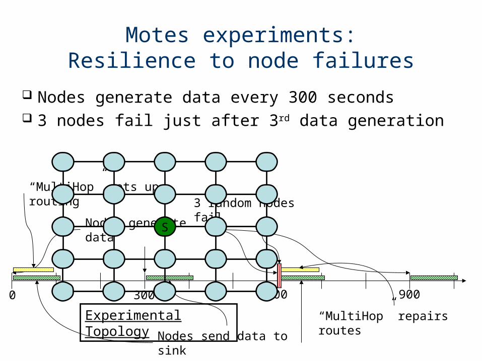
Motes experiments:Resilience to node failures
Nodes generate data every 300 seconds 3 nodes fail just after 3rd data generation
0 300 600 900
Nodes generate data
“ MultiHop” sets up routing
“ MultiHop” repairs routesNodes send data to
sink
3 random nodes fail
S
Experimental Topology

Motes experiments:Resilience to node failures
1st generation: GC faster, MH takes time to setup routes2nd generation: routing already setup, MH very fast
3rd generation: MH needs to repair routes
0 300 600 900
Nodes generate data
“ MultiHop” sets up routing
“ MultiHop” repairs routes
Nodes send data to sink
3 random nodes fail

Conclusions
Data persistence in sensor networks: First distributed channel codes (GC) Protocol requires minimal configuration Is robust to node failures
Simulations and experiments on micaz motes show: GC achieves complete recovery faster GC recovers more partial data at any
time

Received codewords
Iterative Decoding
x1 x3
x5 x2
x1 x3
x4
x3
Recovered symbols
Unused codewords
• 5 original symbols x1 … x5
• 4 codewords received
• Each codeword is XOR of component original symbols

Online Decoding at the Sink
x1
Recovered Symbols
x6
x3
Undecoded codewords
x2⊕x5
Sink
New codeword
x2⊕x6
x1
Recovered Symbols
x6
x3
Undecoded codewords
x2
=
x6
⊕
x2⊕x5
x5
=
x2
⊕
x2⊕x6
x5
Sink
x2


