
115
CHAPTER 6
GROUNDWATER EXPLORATION
6.1 INTRODUCTION
Water is one of the m
water is one of the prerequisites for development and industrial growth. In areas where
surface water is not available, groundwater constitutes significant part of active fresh
water resources of the world and is obviously dependable source for all the needs. The
stress on water resources started due to exploding population, irrigation, domestic and
industrial demands. The finite water resources are being explored to quench the thirst
of millions of the populace. Although the groundwater resources are widely
distributed, nature does not provide groundwater at the places of our choice. The
occurrence and distribution of groundwater resources are confined to certain geological
formations and structures. The groundwater at all locations may not be directly used if
the quality of water is poor. All these problems can be solved using proper exploration
techniques. The proper exploration of groundwater resources involves apart from
source location, the well design and construction. These are all an integral part of the
scheme of exploitation and management.
6.2 GROUNDWATER EXPLORATION
Groundwater exploration in past years has reached a place of importance to the
world and supplying groundwater to the needy is most precious of all. Prospecting for
water is essentially a geological problem and the geophysical approach is dependent on
the mode of the geological occurrence of water. It needs a lot of information on various
aspects such as geology, stratigraphy, geomorphology, geophysical techniques, etc.
Geology is the most important consideration, as different rock types will generally
have a distinctive porosity and permeability. Knowledge of stratigraphy is essential to
know the position and thickness of water-bearing horizons and the continuity of
confining beds are of particular importance in groundwater exploration. Structural
geology is used in conjunction with stratigraphy to locate water-bearing horizons
which have been displaced by earth movements. Structural studies are also used to
locate weathered, fractured, faulted and jointed patterns in rock formations. Remote
sensing techniques are particularly helpful in many geomorphic and structural studies
related to hydrology. The remote sensing data are found extremely useful in identifying

116
the various geologic, geomorphic units, structures such as faults, lineaments, joints,
fractures, folds and drainage which are important as they control the movement and
occurrence of groundwater. Geomorphology is indispensable in studying the
occurrence of subsurface water in areas of late Pleistocene to recent deposits. After a
thorough study of the satellite imagery and geomorphology map, a field check is
highly necessary to know the geomorphological features to assess the groundwater
potential. The geomorphic units such as pediments, flood plains, drainage pattern, soil
types and lineaments which primarily control the occurrence, movement and potential
of groundwater have to be investigated in detail.
The groundwater potential of an area mainly depends on the hydrogeological
set up, for which a detailed and systematic hydrogeological survey is a prerequisite.
Well inventory study is very important in any groundwater exploration programme.
Especially in hard rock terrain groundwater confines to the weathered mantle, joints
and fractures. The weathering thickness, joint and fracture system of the area ought to
be studied in depth. Water level measurements and water level fluctuation studies are
the important factors in the assessment of groundwater potential. Only by a systematic
hydrogeological study, the groundwater abstracting structures such as open well, bore
well, tube well have to be finalised. The recharge and discharge areas ought to be
identified. The fluvial hydrological studies such as the river and stream flows, whether
it is perennial and other details are important in quantifying the potential.
Geophysical methods such as electrical, electromagnetic, seismic and gravity
are used to explore the groundwater. Geophysically, the location of groundwater may
be determined in three ways: direct, stratigraphic and structural (Bhattacharya and
Patra, 1968; Elijah A. Ayolabi, 2005). The stratigraphic method which is relevant to
this study implies locating water-bearing formations through distinguishing physical
properties imparted by the presence of water, giving rise to electrical resistivity
contrasts. The electrical resistivity methods give fairly accurate results in groundwater
investigation. Electrical resistivity methods assumed considerable importance in the
field of groundwater exploration (Pal and Majumdar, 2001; Majumdar and Pal, 2005;
Narayanpethkar et al., 2006) because of its inexpensive, easy operation and its capacity
to identify between fresh and saline water zones, the method is used worldwide. The
resistivity methods are used successfully to estimate the thickness of the formation and
also the electrical nature of the formation which provides useful information regarding
117
the groundwater potentialities (Griffiths and King, 1965; Parasins, 1966; Balakrishna,
1980).
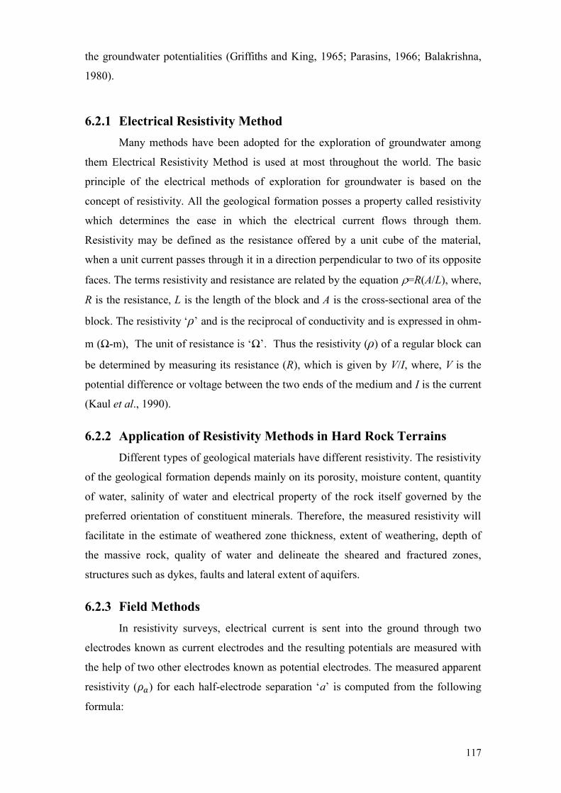
6.2.1 Electrical Resistivity Method
Many methods have been adopted for the exploration of groundwater among
them Electrical Resistivity Method is used at most throughout the world. The basic
principle of the electrical methods of exploration for groundwater is based on the
concept of resistivity. All the geological formation posses a property called resistivity
which determines the ease in which the electrical current flows through them.
Resistivity may be defined as the resistance offered by a unit cube of the material,
when a unit current passes through it in a direction perpendicular to two of its opposite
faces. The terms resistivity and resistance are related by the equation =R(A/L), where,
R is the resistance, L is the length of the block and A is the cross-sectional area of the
block. The resistivity -
m ( -m), The unit of resistance Thus the resistivity ( ) of a regular block can
be determined by measuring its resistance (R), which is given by V/I, where, V is the
potential difference or voltage between the two ends of the medium and I is the current
(Kaul et al., 1990).
6.2.2 Application of Resistivity Methods in Hard Rock Terrains
Different types of geological materials have different resistivity. The resistivity
of the geological formation depends mainly on its porosity, moisture content, quantity
of water, salinity of water and electrical property of the rock itself governed by the
preferred orientation of constituent minerals. Therefore, the measured resistivity will
facilitate in the estimate of weathered zone thickness, extent of weathering, depth of
the massive rock, quality of water and delineate the sheared and fractured zones,
structures such as dykes, faults and lateral extent of aquifers.
6.2.3 Field Methods
In resistivity surveys, electrical current is sent into the ground through two
electrodes known as current electrodes and the resulting potentials are measured with
the help of two other electrodes known as potential electrodes. The measured apparent
resistivity ( ) for each half- a lowing
formula:
118
where, is apparent resistivity, K is the factor depending on the
geometry of electrode configuration, V is the voltage measured across potential
electrodes and I is the current sent into the ground. The apparent resistivity for a given
electrode separation may vary within wide limits depending upon the nature of surface
material. The direction of electrode spread in relation to anisotropic characters and lateral
inhomogeneities etc. The apparent resistivity map for a given electrode spacing indicates
the variation of resistivity in the subsurface layer with a thickness approximately equal to
electrode spacing (Zohdy et al., 1974). There are two main variations of resistivity
surveys, namely profiling and vertical Electrical Sounding (VES). Profiling is used to
determine the lateral variation of resistivity from area to area, whereas VES is used to
investigate the vertical variations of rock strata in a given location.
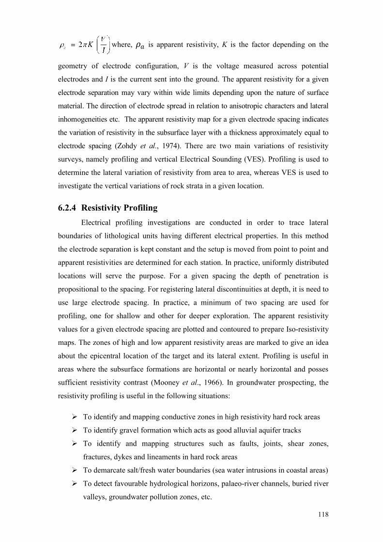
6.2.4 Resistivity Profiling
Electrical profiling investigations are conducted in order to trace lateral
boundaries of lithological units having different electrical properties. In this method
the electrode separation is kept constant and the setup is moved from point to point and
apparent resistivities are determined for each station. In practice, uniformly distributed
locations will serve the purpose. For a given spacing the depth of penetration is
propositional to the spacing. For registering lateral discontinuities at depth, it is need to
use large electrode spacing. In practice, a minimum of two spacing are used for
profiling, one for shallow and other for deeper exploration. The apparent resistivity
values for a given electrode spacing are plotted and contoured to prepare Iso-resistivity
maps. The zones of high and low apparent resistivity areas are marked to give an idea
about the epicentral location of the target and its lateral extent. Profiling is useful in
areas where the subsurface formations are horizontal or nearly horizontal and posses
sufficient resistivity contrast (Mooney et al., 1966). In groundwater prospecting, the
resistivity profiling is useful in the following situations:
To identify and mapping conductive zones in high resistivity hard rock areas
To identify gravel formation which acts as good alluvial aquifer tracks
To identify and mapping structures such as faults, joints, shear zones,
fractures, dykes and lineaments in hard rock areas
To demarcate salt/fresh water boundaries (sea water intrusions in coastal areas)
To detect favourable hydrological horizons, palaeo-river channels, buried river
valleys, groundwater pollution zones, etc.

119
Determining the direction and intensity of joints and fractures (Murali
Sabnavis and Patangay, 1998)
In general, the low resistivity zones in hard rock areas and a higher resistivity
zone in sedimentary formations help to distinguish clay beds from sand beds. Fault
zones and structurally disturbed zones also show relatively low resistivity.
6.2.5 Vertical Electrical Sounding
VES method is used to investigate the vertical variation in electrical property of
the formation. In resistivity sounding method the centre of the electrode configuration
is kept fixed and the distance between current electrodes called the electrode separation
is increased in steps and measurements are made for each electrode separation. The
depth of penetration increases with the increase of electrode separation. The apparent
resistivity values obtained with increasing values of electrode separation are used to
estimate the thickness and resistivities of the subsurface formations. The measured
resistivity values can be correlated with vertical geological sections.
6.2.6 Electrode Configuration
In the exploration of groundwater by resistivity methods, there are number of
ways of setting up of current and potential electrodes. The choice of an array and the
distance between the electrodes is very important for obtaining the best possible
information on the subsurface geology of a given area. Keller and Frischnecht (1966)
have described different configurations viz, Schlumberger, Wenner, Dipole Dipole,
Trielectrode, Lee-partitioning, etc. The Schlumberger method in particular has
practical, operational and interpretational advantages over the rest of the methods
(Bhimasankaram, 1977). The maximum current electrode spacing depends on the depth
to be investigated in a given situation.
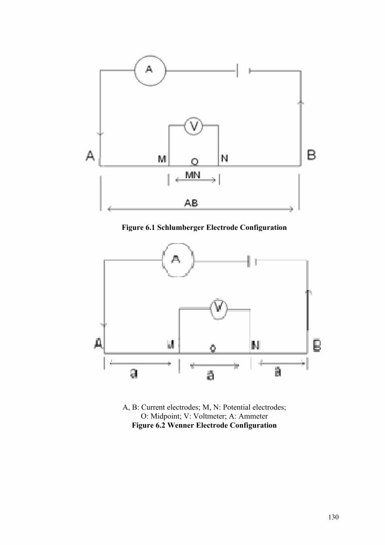
6.2.7 Schlumberger Electrode Configuration
The Schlumberger configuration is most widely used for quantitative
interpretation in VES. Schlumberger originally proposed this electrode arrangement.
Four electrodes are placed symmetrically along a common line with the outer two
serving as current electrodes and the inner two as potential electrodes. The inner pair of
potential electrodes (MN) is located at the centre of the array and the separation
between them is small compared to the current electrode distance (AB), usually less

120
than one-fifth of the current electrode distance (Fig. 6.1). The apparent resistivity
values obtained with this array are attributed to the midpoint of configuration, which is
called as
completely uniform earth is given by the formula (Keller and Frischnecht, 1966)
where, = apparent resistivity, V = potential difference between potential
electrodes, I = current flowing, AB = current electrodes, MN = potential electrodes.
6.2.8 Wenner Configuration
In this configuration, four equally spaced and collinear electrodes are used. The
outer current electrodes (A and B) provide current to the ground, whereas the inner two
potential electrodes (M and N) are used to measure the voltage drop due to earth
held fixed and all four
electrodes being separated by equal distances at all times (Fig. 6.2). The apparent
resistivity for this type of electrode arrangement is given by (Keller and Frischnecht,
1966) the formula:
a 2V
aI
where, a = Apparent resistivity, a = Distance between two electrodes,
V = Potential difference between potential electrode and I = Current sent into the
ground.
6.2.9 Resistivity in Hard Rock Terrains
The typical hydrogeological section of a hard rock terrain consists of a soil zone
followed by a weathered zone are overlying bedrock, which is fractured to varying
degrees. Weathered zone is more permeable than bedrock and an appreciable portion of
the available groundwater is stored in that zone. The fractures, joints and other openings
present in the rock act as conduits for circulation of groundwater rather than for
accumulation. However, these structures under favourable situations act as potential zones
of groundwater accumulation. According to Narasimhan (1972), the occurrence of
groundwater beyond a depth of about 70 m below ground level is not significant due to the
tendency of joints, fissures and other such openings to tightly close down at that depth.

121
However, there are several instances of potential groundwater accumulation at much
deeper levels.
The thickness of water-bearing zones of weathered and semiweathered layer is
variable. Their resistivities vary from 30 to 200 -m. Such low resistivity regions indicate
potential groundwater zones. Depending on the degree of jointing, granite with full of
joints and cracks filled with water may show resistivities of the order of 50 to 250 -m
(Ramachandra Rao, 1975). Ramanujacharya (1974) and Balakrishna (1980) have given the
following general resistivity range for granitic terrains:
Formation Representative Resistivity Range ( -m) Highly weathered layer 20 50
Semiweathered layer 50 120
Fractured and jointed granites 120 200
Hard granites >200
6.3 RESISTIVITY SURVEYS IN THE STUDY AREA
Fifty-one VES have been carried out at different parts of the study area using
Schlumberger method of electrode configuration by using Aqua Meter to determine the
groundwater potential zones of the study area. The resistivity meter is placed at an
observation station, which is suitable for spreading the cable on either direction. The
electrodes for measuring on the potential difference are placed on either side of the
chosen point. Two current electrodes are driven into the ground to 10 to 15 cm deep on
either side of the centre. These current electrodes are connected to instrument. The
electrical connections and separations are checked before each measurement. The
apparent resistivity value is determined by sending current (I) into the ground and
measuring the potential drop (V/I) ratio multiplied by configuration current (K). The
electrode spacing (AB) is then increased and the corresponding apparent resistivity
value is measured. The operation is repeated again and again whereas the current
electrodes are extended further away from the centre, keeping the potential electrodes
(porous pots) stationary. When the potential difference value becomes very small, the
distance between the potential electrodes are increased. After this increase, the
apparent resistivity can be measured for increasing current electrode separations using
the larger potential electrode separation. The apparent resistivity with Schlumberger
electrode configuration is computed by using the formula:

122
2 2
a
where, AB = Distance between current electrodes, MN = Distance between
potential electrodes, V = Voltage measured across potential electrodes and I = Current
flowing.
The VES data have been used to determine the thickness and resistivity values
of weathered, semiweathered and fractured layers.
6.3.1 Interpretation of Field Curves
The interpretation of resistivity sounding data in terms of thickness and
resistivity of the underlying beds with reasonable limit of accuracy is difficult problem.
For a correct interpretation of geoelectrical sounding curves, a sound knowledge in
geology of the area, some borehole data and considerable practical experience are
essential. Geoelectrical sounding curves are interpreted qualitatively in terms of
geology of the area. The qualitative methods of interpretation can be used only for
preliminary interpretation as explained by Mooney et al. (1966), Bhattacharya and
Patra (1968). There are several methods of interpretation of VES data, in the present
study curve matching technique is used.
6.3.2 Curve Matching Method
The curve matching technique is used to determine the layer parameters from
the VES curves. The field curves are matched with standard curves to get the layer
parameters. Several such standard curves are available viz, Mooney et al. (1966),
Zohdy (1968) and Rajkswterstaat (1975). In this study layer parameters have been
obtained by using IPI2WIN ware. The layer parameters obtained by the analysis
are presented in the Table 6.1. The VES curves obtained are of three layered, the top
most layers have the resistivity values ranging from 12 to 65 -m and its thickness
ranges 1.2 to 1.9 m. This variation in the resistivity values due to the local conditions
such as, soil moisture content. The resistivity of the second layer varies between 12 to
156.2 -m and the thickness ranges between 4.5 to 15.5 m, this layer corresponds to
weathered layer. The third layer generally represents the semiweathered/fractured
rocks exhibiting resistivity values ranges from 36 to 385 -m. In some cases, the third
layer represents the compact hard bed rock.

123
6.3.3 Iso-Resisitivity Maps
Iso-resistivity maps of the study area prepared by contouring the apparent
resistivity values, corresponding to the electrode spacing (AB/2) of 30 and 60 m by
using ArcGIS 9.3 software. These maps are helpful in delineating low apparent
resistivity zones and are favourable locations for groundwater storage, provided the
weathered layer is sufficiently thick and permeable. The apparent resistivity values
ranges from 14 to 65 -m and 45 to110 -m (Table 6.1) at 30 and 60m electrode
spacing, respectively. The Iso-resistivity maps for both 30 and 60 m electrode spacing
indicates (Maps 6.1 and 6.2) that the high resistivity values have been found in
northern (Nandi), northeastern (Jangamakote), western (Devanahalli), southern
(Sarjapura and Dommasandra) and southeastern (Sulibele) parts of the study area. The
high resistivity values in these areas are due to the presence of massive bedrock at
shallow depth and absence of water-bearing zones. The remaining part of the study
area have moderate to low apparent resistivity and these regions are promising zones
for groundwater development. The north and eastern part of the study area found
patches of lateritic outcrops. In these areas a sudden fall in apparent resistivity,
indicates the contact zone of lateritic and basement massive weathered rock found
gravel layer, it shows a moderate to good amount of groundwater potential and are
prospective zones for further development in the study area.
6.3.4 Iso-Thickness Maps
The thickness of soil and weathered layers are also very important from the
point of groundwater potential zones, as the percolation of rainwater is mainly
controlled by these layers. The thickness of the first (h1) and second (h2) layers are
varies from 1.2 to 1.9 m with an average of 1.65 m. The thickness of second layer
varies from 4.5 to 15.5 m and an average of 8.23 m. The variation in the thickness
mainly due to the variation in lithology and landforms. The Iso-thickness map of h1
and h2 (Maps 6.3 and 6.4) shows the anomalous zones in northern, western, central,
southern and southeastern parts of the study area. The lithologies of these anomalous
zones are weathered gneisses and granites. They have more chance for infiltration of
rainwater and are the potential zones of groundwater.
124
6.3.5 Total Longitudinal Conductance Map
Determination of total longitudinal conductance (S) provides an important
check on the curve interpretation and can be used for the preparation of S-map. The
total longitudinal conductance has been determined from the slope of the terminal
branch of the sounding curve called S-line, rising at an angle of 45 to the AB/2 axis
(Zohdy et al., 1974). If the S-line is extended back to intersect the a = 1 -m line,
then the intersect point on the x-axis is equal to S, the total longitudinal conductance
above the final layer S in mohs or Siemens (Murali
Sabnavis and S
the slope of this line (Keller and Frischnecht, 1966). When a number of layers are
involved in a geo S
S = S1 + S2 + S3 + S4 + S5 + , where, S1 = h1/ 1
In this S IPI2WIN software and values
are presented in the Table 6.1. The longitudinal conductance in the study area varies
from 0.35 to 0.96 mhos. The spatial variation of S-map indicates that the high values
are noticed in northern, western, central, southern and southeastern parts of the study
area indicating good aquifer conditions (Map 6.5). The increase in the S values
indicates the decrease in the overall resistivity of the formations and increase in the
thickness of overburden. High values of S can be considered as an important index of
groundwater potential.

125
Table 6.1 Layer Parameters for the VES Data
Sl. No.
Location
Resistivity of Different Layers ( -m)
Thickness of Layers (m)
Total Thickness
(m)
S (Mhos)
Apparent Resistivity at
1 2 3 h1 h2 30 m 60 m
1 Nandhi 36.23 64.32 125 1.7 8.2 9.9 0.85 54 64
2 Bendiganahalli 54.2 75 120 1.9 7.35 9.25 0.85 45 65
3 Siddlaghatta 64 35 120 1.9 15.5 17.4 0.96 35 70
4 Gottigere 45 23 225 1.6 12.5 14.1 0.86 45 54
5 Meluru 55 65 145 1.7 9.6 11.3 0.75 54 65
6 Vijayapura 52 15.2 135 1.7 8.2 9.9 0.84 36 65
7 Chikkaballapura 27.12 45.32 365 1.8 7.2 9 0.8 45 65
8 Avathi 65 84 385 1.8 11.2 13 0.54 23 100
9 Jangamakote 65 156.2 78 1.9 9.3 11.2 0.45 56 58
10 Venkatapura 25 23 112 1.75 8.5 10.25 0.56 14 45
11 Devanahalli 35 24 36 1.2 8.5 9.7 0.65 28 65
12 Keshavara 21 45.23 128 1.7 8.36 10.06 0.45 42 75
13 Mallur 54.2 75 120 1.9 7.35 9.25 0.85 45 65
14 Anneswara 21 45 184 1.5 6.84 8.34 0.75 45 55
15 Sugatta 45 84 165 1.6 7.24 8.84 0.84 54 65
16 Hosahudya 36 54 84 1.2 6.84 8.04 0.42 45 74
17 Kogilu 26 12 225 1.9 9.5 11.4 0.65 36 75
18 Sulibele 40 20 132 1.3 10.4 11.7 0.84 45 110
19 Bagalur 24 45 112 1.2 8.6 9.8 0.96 42 96
20 Kodigehalli 25 42 84 1.3 7.5 8.8 0.35 24 65
21 Hunsamaranahalli 24 36 41 1.4 7.5 8.9 0.54 21 65
22 Patrenahalli 22 25 36 1.5 7.2 8.7 0.52 32 75
23 Keshavapura 26 12 45 1.8 8.2 10 0.62 36 56
24 Dommasandra 22 45 52 1.9 7.3 9.2 0.85 45 75
25 Mugulur 28 65 45 1.7 8.2 9.9 0.95 36 84
26 Keshavapura 23 45 65 1.6 7.2 8.8 0.85 45 75
27 Mangammanapalya 18 23 45 1.6 7.5 9.1 0.75 36 84
28 K. Narayanapura 20 33 65 1.7 8.2 9.9 0.45 45 95
29 Muddenahalli 24 45 85 1.9 8.5 10.4 0.63 25 58

126
Sl. No.
Location
Resistivity of Different Layers ( -m)
Thickness of Layers (m)
Total Thickness
(m)
S (Mhos)
Apparent Resistivity at
1 2 3 h1 h2 30 m 60 m
30 Kanithahalli 28 52 75 1.8 7.5 9.3 0.85 45 85
31 Begur 22 45 65 1.5 7.2 8.7 0.85 45 75
32 Sarjapura 15 25 45 1.4 6.8 8.2 0.65 54 85
33 Mandur 23 45 78 1.9 7.5 9.4 0.75 45 96
34 Nagavara 22 36 75 1.8 8.5 10.3 0.65 36 85
35 Nagenahalli 22 36 85 1.7 7.5 9.2 0.58 45 95
36 Gantiganahalli 16 29 75 1.6 8.5 10.1 0.45 36 85
37 Jakkur 22 36 45 1.7 9.2 10.9 0.65 22 85
38 Budigere 22 36 75 1.8 8.5 10.3 0.65 45 75
39 Devaganahalli 14 18 45 1.8 7.5 9.3 0.65 25 75
40 Doddagubbi 12 22 45 1.5 7.3 8.8 0.45 22 45
41 Hoshigal 25 65 56 1.6 4.5 6.1 0.45 23 75
42 Yelahanka 18 24 56 1.7 7.5 9.2 0.65 28 48
43 Singasandra 18 35 78 1.8 9.6 11.4 0.65 25 65
44 Bilekahalli 22 27 84 1.7 6.5 8.2 0.65 35 75
45 Bidarahalli 16 42 75 1.8 7.8 9.6 0.85 45 84
46 Navarthna Agrahara 22 28 85 1.6 7.4 9 0.75 65 78
47 Hosakote 28 45 85 1.8 8.5 10.3 0.75 65 85
48 Chikkajala 34 64 124 1.6 7.5 9.1 0.85 36 45
49 Laksandra 21 36 75 1.7 7.8 9.5 0.65 45 55
50 Karahalli 35 22 45 1.5 8.5 10 0.54 35 84
51 Jakkur 18 24 65 1.7 9.8 11.5 0.96 45 72


129
Map 6.5 Iso-Longitudinal Conductance Map the Study Area
130
Figure 6.1 Schlumberger Electrode Configuration
A, B: Current electrodes; M, N: Potential electrodes;
O: Midpoint; V: Voltmeter; A: Ammeter Figure 6.2 Wenner Electrode Configuration


