Geostatistical Time-lapse Seismic Inversion
Valter Miguel Dos Santos Proença
Thesis to obtain the Master of Science Degree in
Petroleum Engineering
Supervisor: Professor Leonardo Azevedo Guerra Raposo Pereira.
Examination Committee
Chairperson: Professor Amílcar de Oliveira Soares
Supervisor: Professor Leonardo Azevedo Guerra Raposo Pereira
Member of the Committee: Professor Maria João Correia Colunas Pereira
November 2016

i
Abstract
With the decrease of the oil price and of new discoveries, it is not only important to use new exploration
and production methods and technologies but improve and optimize the monitoring of hydrocarbon
reservoirs during production. This leads to a more efficient decision making process, while reducing risks
and increasing oil recovery factors. Although a relatively new area, nowadays there are already some
methodologies that invert time-lapse seismic data, based on a Deterministic or Bayesian inversion
framework. This thesis introduces a new iterative geostatistical time-lapse seismic inversion methodology.
The objective of this work is the development and implementation of a new methodology able to reproduce
the changes of the elastic properties during production time integrating time-lapse seismic reflection data
from the different acquisition times. This new approach was tested and implemented in a realistic synthetic
dataset Stanford VI-E. The results show a good reproduction of the changes in the elastic properties of
interest. It was also concluded, during the comparison of the both methods used in this work, that the
horizontal time-slices of elastic differences computed from the conventional global elastic inversion do not
reproduce the spatial continuity of the elastic differences values. Otherwise the proposed workflow,
reproduces the spatial continuity pattern of these changes with improved accuracy.
Keywords: Reservoir characterization, geostatistical time-lapse inversion, elastic changes, 4D seismic
data, geostatistical modeling

ii
.
iii
Resumo
Com a diminuição do preço do petróleo e de novas descobertas, é importante não só usar novos
métodos e tecnologias de exploração e produção, mas melhorar e otimizar o monitoramento de
reservatórios de hidrocarbonetos durante a produção. Isto era conduzir a um processo de tomada de
decisão mais eficiente, reduzindo os riscos e aumentando os fatores de recuperação dos hidrocarbonetos.
Embora estejamos presentes numa área relativamente nova, hoje em dia já existem algumas metodologias
que invertem dados sísmicos 4D, com base em metodologias de inversão determinísticas e Bayesianas.
Esta tese apresenta uma nova metodologia de inversão de sísmica interativa 4D geostatistica. O objetivo
deste trabalho é o desenvolvimento e implementação de um novo procedimento capaz de reproduzir as
alterações das propriedades elásticas durante o tempo de produção integrando dados de reflexão sísmica
4D a partir dos diferentes tempos de aquisição. Esta nova abordagem foi testada e implementada num
conjunto de dados sintéticos realistas Stanford VI-E. Os resultados mostram uma boa reprodução das
alterações das propriedades elásticas de interesse. Conclui-se ainda, durante a comparação de ambos os
métodos utilizados no âmbito deste trabalho, que as fatias de tempo horizontais das diferenças elásticas
calculadas a partir da inversão elástica convencional global, não reproduzem a continuidade espacial dos
valores das diferenças elásticas reais. No caso contrario, o proposto método desta tee, reproduz o padrão
de continuidade espacial dessas mudanças com maior precisão.
Palavras-chave: caracterização do reservatório, inversão 4D geostatistica, mudanças elásticas, sísmica
4D,modelação geostatistica.

iv
v
Table of Contents
Abstract ............................................................................................................................................... I
Resumo ............................................................................................................................................. III
Table of Contents ................................................................................................................................ V
List of Figures .................................................................................................................................... VI
List of Tables ...................................................................................................................................... X
Acronyms .......................................................................................................................................... XII
Chapter 1: Introduction ........................................................................................................................ 1
1.1 Motivation ............................................................................................................................. 1
1.2 Objectives ............................................................................................................................. 2
1.3 Structure of the thesis ........................................................................................................... 3
Chapter 2: Geostatistical Models for Earth Science Applications.......................................................... 5
2.1 Spatial continuity analysis .......................................................................................................... 5
2.2 Variograms ................................................................................................................................ 6
2.3 Direct Sequential Simulation and co-Simulation (DSS and Co-DSS) ........................................ 10
2.4. Direct Sequential co-simulation with joint probability distributions ............................................ 13
Chapter 3: Integration of Seismic data In Reservoir Modeling Characterization .................................. 15
3.1 Seismic inversion .................................................................................................................... 15
3.2 Geostatistical Seismic Inversion .............................................................................................. 18
3.3 Time-Lapse Seismic ................................................................................................................ 19
3.4 Time-lapse seismic inversion ................................................................................................... 20
Chapter 4: Methodologies ................................................................................................................. 23
4.1 Geostatistical elastic inversion: Global Elastic Inversion ........................................................... 23
4.2 Geostatistical Time-lapse Inversion ......................................................................................... 24
Chapter 5: Case Study ...................................................................................................................... 29
5.1 Data Description ...................................................................................................................... 29
5.1.1 Structure and stratigraphy ................................................................................................. 32
5.1.2 Exploratory data analysis .................................................................................................. 34
vi
5.1.3 Parameterization .............................................................................................................. 38
5.2 Geostatistical Time-lapse Inversion ......................................................................................... 40
5.2.1 Synthetic seismic .............................................................................................................. 40
5.2.2 Acoustic and Elastic Impedance Models ........................................................................... 42
5.2.3 Histograms, Bi-plots and Statistics .................................................................................... 45
5.3 Comparison between geostatistical elastic inversion and geostatistical time-lapse inversion
methodologies ................................................................................................................................... 50
5.3.1 Differences between seismic ............................................................................................ 50
5.3.2 Acoustic and Elastic Differences ....................................................................................... 52
Chapter 6: Discussion, Conclusions and Future work ........................................................................ 55
References ....................................................................................................................................... 59
Appendix A ......................................................................................................................................... 1
vii
List of Figures
Figure 1-Seismic near-stack amplitude differences between the different times of acquisition during
production. Differences from (from the left to the right): base survey and (10 years of production, 10 and 25
of production and 25 and 30 years of production). .................................................................................... 1
Figure 2 - Graphic representation of a spherical model (Pereira, 2014). .............................................. 8
Figure 3 - Graphic representation of an exponential model (Pereira, 2014). ........................................ 9
Figure 4 - Graphic representation of a Gaussian model (Pereira, 2014). ............................................. 9
Figure 5 - Sampling of global probability distribution Fz (z), by intervals defined by the local mean and
variance of z(xu): The value � ��*corresponds to the local estimate z(xu)*. The simulated value z(xu)* is
drawn from the interval of Fz (z) defined by � (� ��*, �2(��)) ( adapted from Soares 2001). ............... 11
Figure 6 - Schematic of possible work flows in seismic inversion for reservoir properties leading to
multiple realizations of reservoir properties conditioned to seismic data, the rock - physics models, and the
model of spatial continuity imposed by geology.(a,b) Two variations of sequential work flow. (c)
Simultaneous Bayesian inversion work flow. Data come in at various stages, including seismic data for
inversion, well-log data, cores and thin sections when available, and geologic data from outcrops (Bosh et
al., 2010). .............................................................................................................................................. 16
Figure 7 - Schematic representation of the GEI workflow (Azevedo, 2013). ....................................... 24
Figure 8 - Graphic representation of the geostatistical time-lapse inversion. ...................................... 27
Figure 9 -Real models of acoustic impedance from each year of acquisition, T0, T10, T25 and T30
respectively. ........................................................................................................................................... 29
Figure 10- Real models of elastic impedance from each year of acquisition, T0, T10, T25 and T30
respectively. ........................................................................................................................................... 30
Figure 11 - Representation of the partial angle stacks form seismic reflection data, 0º, 10º, 20º, 30º and
40º respecively. ..................................................................................................................................... 31
Figure 12 – Representation of the stack wavelets correspondent to the 5 angle stacks. .................... 32
Figure 13 – Perspective view of the Stanford VI-E top structure: view from SW (left), view from SE (right).
The color indicates the depth to the top (Lee & Mukerji 2012). ................................................................ 33
Figure 14 - Histogram representing the number of acoustic impedance samples per class of the well-log
data o each year of acquisition. .............................................................................................................. 34
Figure 15 - Histogram representing the number of elastic impedance samples per class of the well-log
data o each year of acquisition. .............................................................................................................. 35

viii
Figure 16 - Well-log data bi- histogram of each acquisition time, expressing the relation between the two
properties of interest (AI and EI). ............................................................................................................ 36
Figure 17 - Chosen main direction of AI for modeling, with exponential model................................... 37
Figure 18 - Chosen main direction of EI for modeling, with exponential model................................... 37
Figure 19 - Illustration of the simulation mask, T1T2, T2T3 respectively. The red color represents the
places to be simulated. .......................................................................................................................... 39
Figure 20 - Inverted residual models from T10, T25, and T30 respectively. ....................................... 39
Figure 21 - Global correlation coefficient evolution between synthetic and real seismic reflection data for
the four available seismic vintages using geostatistic time-lapse inversion method. ................................ 40
Figure 22 - Comparison of all angle stacks between the real seismic (left), the synthetic seismic from
the best-fit models (Center) and the Synthetic seismic computed from the mean of the models from the last
iteration. The seismic results are related to the different times of acquisition divided by rows, being the first
related to the year 0 and the last to the year 30. ..................................................................................... 41
Figure 23 - Comparison of the near angle stack between the real acoustic impedance models (Right),
the simulated best-fit acoustic impedance models (Center) and the mean of the simulated acoustic models
computed from the last iteration. The first line is related to the year 0 and the other too years 10, 25, and 30
respectively. ........................................................................................................................................... 43
Figure 24 - Comparison of the near angle stack between the real elastic impedance models (Right), the
simulated best-fit elastic impedance models (Center) and the mean of the simulated elastic models
computed from the last iteration. The first line is related to the year 0 and the other too years 10, 25, and 30
respectively. ........................................................................................................................................... 44
Figure 25 - Acoustic impedance histograms from the well-log data of each year against the histograms
from the best-fit models of each acquisition year. ................................................................................... 46
Figure 26 - Elastic impedance histograms from the well-log data of each year against the histograms
from the best-fit models of each acquisition year. ................................................................................... 47
Figure 27 - Bi-histograms of well-log data against best-fit models of each year, expressing the relation
between the two properties of interest, AI and EI. ................................................................................... 48
Figure 28 - Comparison the near angle stacks between the real seismic (left column), the Synthetic
seismic computed from the mean of the models from the last iteration using Geostatistic Time-lapse
inversion (center column) and the synthetic seismic from the best-fit models using GEI (right column). The
seismic results are related to the different times of acquisition divided by lines, being the first related to the
year 0 and the last to the year 30. .......................................................................................................... 51

ix
Figure 29 - Acoustic impedance differences from: the real (left), geostatistical time lapse inversion
(middle) and global elastic inversion (right) for the T0-T10, T10-T25, and T25-T30 years respectively .... 52
Figure 30 - Elastic impedance differences from: the real (left), geostatistical time lapse inversion (middle)
and global elastic inversion (right) for the T0-T10, T10-T25, and T25-T30 years respectively .................. 53

x
List of Tables
Table 1 - Values of the modeled variograms. .................................................................................... 37
Table 2 - Values of the modeled variograms ..................................................................................... 38
Table 3 – Acoustic impedance main statistics of well-log data and best-fit models related to each year.
.............................................................................................................................................................. 49
Table 4 – Elastic impedance main statistics of well-log data and best-fit models related to each year 49

xi

xii
Acronyms
AI: Acoustic Impedance
Cdf: Cumulative distribution function
Co-DSS: Direct Sequential co- Simulation
DSS: Direct Sequential Simulation
EI: Acoustic Impedance
GEI: Global Elastic Inversion
Ip: Primary impedance
Is: Secondary impedance
Pdf: Probability distribution function
Vs: Secondary wave velocity
Vp: Primary wave velocity
1
Chapter 1: Introduction
1.1 Motivation
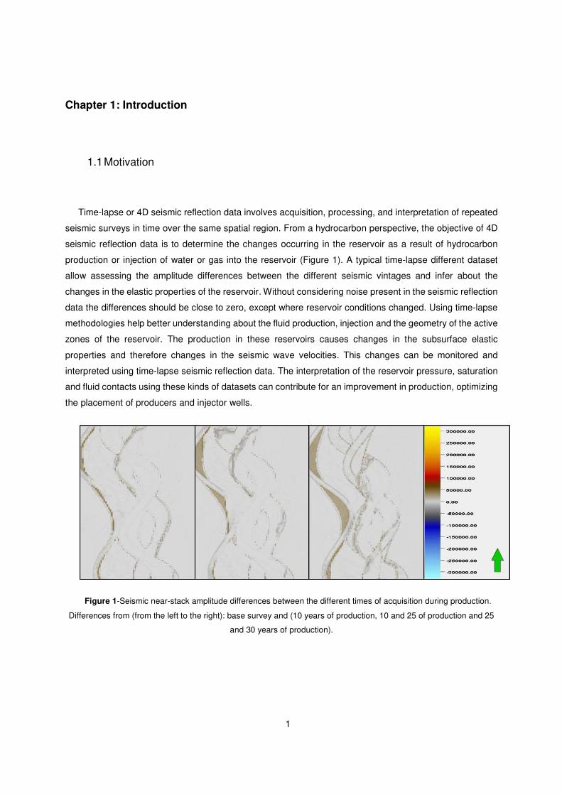
Time-lapse or 4D seismic reflection data involves acquisition, processing, and interpretation of repeated
seismic surveys in time over the same spatial region. From a hydrocarbon perspective, the objective of 4D
seismic reflection data is to determine the changes occurring in the reservoir as a result of hydrocarbon
production or injection of water or gas into the reservoir (Figure 1). A typical time-lapse different dataset
allow assessing the amplitude differences between the different seismic vintages and infer about the
changes in the elastic properties of the reservoir. Without considering noise present in the seismic reflection
data the differences should be close to zero, except where reservoir conditions changed. Using time-lapse
methodologies help better understanding about the fluid production, injection and the geometry of the active
zones of the reservoir. The production in these reservoirs causes changes in the subsurface elastic
properties and therefore changes in the seismic wave velocities. This changes can be monitored and
interpreted using time-lapse seismic reflection data. The interpretation of the reservoir pressure, saturation
and fluid contacts using these kinds of datasets can contribute for an improvement in production, optimizing
the placement of producers and injector wells.
Figure 1-Seismic near-stack amplitude differences between the different times of acquisition during production.
Differences from (from the left to the right): base survey and (10 years of production, 10 and 25 of production and 25
and 30 years of production).
2
Time-lapse studies normally use two or more migrated 3D seismic volumes obtained months or years
apart for the same spatial area. These can consist of stacked data volumes or stacks created from partial
offsets if AVO/AVA aspects are considered. To study and interpret the changes in the seismic volumes,
some different approaches have been done, however none within a geostatistical framework. Geostatistical
modeling and inversion techniques contribute for a better reservoir characterization since they allow the
assessment of the spatial uncertainty of the inferred property. There are several modeling techniques that
allow accessing different levels of detail in the characterization of the reservoir model, however and
regardless of the technique used, there will be always a degree of uncertainty associated with inverse
models that is important to evaluate (Azevedo, 2013). Inverting different vintages of seismic reflection data
separately is not enough since there is no conditioning of the properties changes between each acquisition
time. The main motivation of this work is to have a workable algorithm that with a unique geostatistical
approach, integrate the time-lapse seismic reflection data inverting all times simultaneously, ensuring the
reproduction of the elastic changes in reservoir during production.
1.2 Objectives
The main objective of this Master thesis is the development and implementation of a new iterative
geostatistical time-lapse seismic inversion methodology. The proposed algorithm was tested in the classic
Stanford VI-E reservoir (Lee & Mukerji, 2012). The main objectives of this work may be summarized by the
following:
- Implementation of a new Geostatistical time-lapse seismic inversion methodology.
- Compare the new algorithm results with those obtained by standard geostatistical elastic
inversion (GEI) of the different acquisition times to understand the importance of the joint
inversion.
- Compare the results of the new algorithm with the real synthetic data models of Acoustic
Impedance (AI) and Elastic Impedance (EI) to see the effectiveness of this new method.
- Understand the pros and cons of this new method compared to the ones already in use.
In the developing of this thesis, various computer tools were used the geostatistical modeling software
GeoMS ( CERENA / IST) for modeling the variogram data logs of the wells, the two geostatistical seismic
inversion methodologies were performed using code developed in Matlab® (Math works) and Petrel®
(Schlumberger) for data visualization and manipulation.

3
1.3 Structure of the thesis
This thesis is divided in six chapters:
• The first chapter, introduce the scientific question that led to the research summarized by this
thesis, as well as the objectives to accomplish.
• Chapter II introduces the theoretical background in which the geostatistical model is developed,
and the description of the direct sequential simulation and direct sequential co-simulation
algorithms that are part of the inversion procedures developed under the scope of this work.
• Chapter III gives an overview on the basics of the seismic inversion and the global geostatistic
elastic seismic inversion algorithm that is the base of the proposed methodology of this work. It
is also presented some ideas and studies developed using time-lapse seismic as well as some
historical background.
• Chapter IV describes and illustrates the methodologies of the two workflows tested,
geostatistical elastic inversion (GEI) and geostatistical time-lapse inversion (GTI).
• Chapter V presents the case study and the application of the two methodologies in a realistic
synthetic reservoir, Stanford VI-E, as well the results from those tests.
• Chapter VI show the conclusions taken from this work concerning the limitation and strong points
observed, as well as some discussion about further applications in the practical implementation
of the introduced methodology.

4
5
Chapter 2: Geostatistical Models for Earth Science Applications
2.1 Spatial continuity analysis
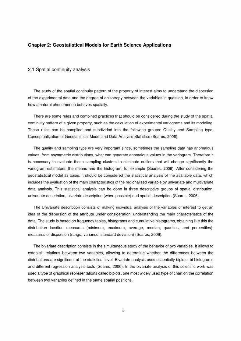
The study of the spatial continuity pattern of the property of interest aims to understand the dispersion
of the experimental data and the degree of anisotropy between the variables in question, in order to know
how a natural phenomenon behaves spatially.
There are some rules and combined practices that should be considered during the study of the spatial
continuity pattern of a given property, such as the calculation of experimental variograms and its modeling.
These rules can be compiled and subdivided into the following groups: Quality and Sampling type,
Conceptualization of Geostatistical Model and Data Analysis Statistics (Soares, 2006).
The quality and sampling type are very important since, sometimes the sampling data has anomalous
values, from asymmetric distributions, what can generate anomalous values in the variogram. Therefore it
is necessary to evaluate those sampling clusters to eliminate outliers that will change significantly the
variogram estimators, the means and the histogram, for example (Soares, 2006). After considering the
geostatistical model as basis, it should be considered the statistical analysis of the available data, which
includes the evaluation of the main characteristics of the regionalized variable by univariate and multivariate
data analysis. This statistical analysis can be done in three descriptive groups of spatial distribution:
univariate description, bivariate description (when possible) and spatial description (Soares, 2006)
The Univariate description consists of making individual analysis of the variables of interest to get an
idea of the dispersion of the attribute under consideration, understanding the main characteristics of the
data. The study is based on frequency tables, histograms and cumulative histograms, obtaining like this the
distribution location measures (minimum, maximum, average, median, quartiles, and percentiles),
measures of dispersion (range, variance, standard deviation) (Soares, 2006).
The bivariate description consists in the simultaneous study of the behavior of two variables. It allows to
establish relations between two variables, allowing to determine whether the differences between the
distributions are significant at the statistical level. Bivariate analysis uses essentially biplots, bi-histograms
and different regression analysis tools (Soares, 2006). In the bivariate analysis of this scientific work was
used a type of graphical representations called biplots, one most widely used type of chart on the correlation
between two variables defined in the same spatial positions.
6
In the study of the spatial distribution of a given variable it is attempted to visualize de variable behavior
in relation to their dispersion in space. It is also intended to make the planning of the basic parameters for
the calculation of variogram, by viewing the spatial arrangement of the experimental variable data and get
a first idea of the spatial dispersion characteristics of the same variable, like anisotropy and
anomalies,(Soares, 2006). There are some situations that need to be taken under account, essentially when
they are characterized by higher values of local variances that imply higher errors in the spatial inference
and especially with greater uncertainty, like for example:
• The higher the extreme values and agglomerates in the same area, the greater is the average
value and the smaller the value of the local variance;
• The higher the extreme values and there is no concentration in the same are, the greater the
average value and the local variance;
• The lower extreme values in this area, the lower the average value unlike the local variance that
tends to increase.
2.2 Variograms
In geostatistics, the variogram (or semi-variogram) describes the spatial relationship between points of
a given attribute Z (x). It is a spatial continuity instrument used to quantitatively represent the change in a
regionalized phenomenon in space, i.e. the variable of interest (Soares, 2006). It is an intrinsic function that
reflect the spatial structure of the phenomenon under study, measuring statistical relationships like the
covariance that exist between samples of successive values of distance (h) between each pair of
experimental data. The variogram is also an increasing function in which the values of the abscissa, vary
until a given value of h, a value known as the variogram range (Soares, 2006).Variograms that have a sill
are associated with stationary regionalized variables, otherwise they are considered non-stationary. Note
that the phenomenon under study can nevertheless be stationary in sub-regions of the area in study.
The estimator of the variogram (Equation 1) provides information on the spatial continuity of the
attributes, at different distances�Z(x + h)�, for various values of h, for the calculation of this estimator. The
centered covariance estimator (Equation 2) provides information of spatial average of the product between
different attributes at different distances�Z(x)Z(x + h))�. These estimators are the geostatistical measures
more often used which represent the correlation between samples(Zα and Zα + h), and can be calculated
by the following expressions (Soares, 2006):
7
γ(h) = 12 E[Z(x) − Z(x + h)]� (1)
C(h) = E�Z(x)Z(x + h) − E�Z(x) E�Z(x + h) (2)
The standard form of covariance, the correlogram (Equation 3), can be defined as the ratio between the
covariance and variogram:
γ(h) = C(0) − C(h) (3)
Variograms are generally anisotropic, but can also be isotropic, representing a different behavior of
spatial correlation in different directions or in a different distance h. This difference in behavior is
representative (in most cases) when we relate variograms of horizontal directions with variograms with
vertical directions. The anisotropy is dependent on the variable or natural system under study. For example,
a given geological layer, should have a higher spatial continuity in the horizontal direction when compared
with the spatial continuity of the vertical direction (Soares, 2006). The opposite phenomenon occurs when
computing experimental variogram from existing well data. In these cases, the vertical direction is more
spatially sampled then in the horizontal direction. As the module of difference between samples (|ℎ|)
increases, the average variation between pairs of samples tends to increase.
Once the variogram is an increasing function, as the module |ℎ| increases, the average variation between
pairs of samples tends to increase as well, until it reaches the range, distance from which it no longer occurs
that increase and the function begins to stabilize. Using the variogram in the main directions, it is possible
to calculate the average dimensions of the body along respective directions (Soares, 2006).
When created the experimental variogram from the set of samples in region of interest it is necessary to
adjust the data to a theoretical model, doing the data modeling through a general mathematical function
that represents the continuity of the spatial variable (Soares, 2006). This stage is very important as it
summarizes the structural characteristics of spatial phenomenon under study, including anisotropy and
degree of continuity of the variable under study.
The practice of geostatistical modeling is limited to the use of a restricted set of functions that covers the
spatial continuity pattern of most natural phenomenon. It is necessary to select the best suited to each case
but essentially those that meet certain conditions: positive definite models that can provide stable solutions.
The positive condition of the models restricts from the beginning, the choice of possible functions for
interpolating the experimental variogram samples. The theoretical models most used variograms are:
Spherical model, Exponential and Gaussian have, all of them, functions of two parameters, namely a Sill($),
which is the superior limit that the variogram values tend as the distance between sampling pares increase,
and the amplitude ( h = a ) of the variogram, that the distance from which the values of the variogram ( %(ℎ))
8
stop to grow and are equal to the sill, that is normally coincident to the variance of the attribute in study. The
amplitude measures the distance from which the values of that attribute begin to show no correlation
between them.
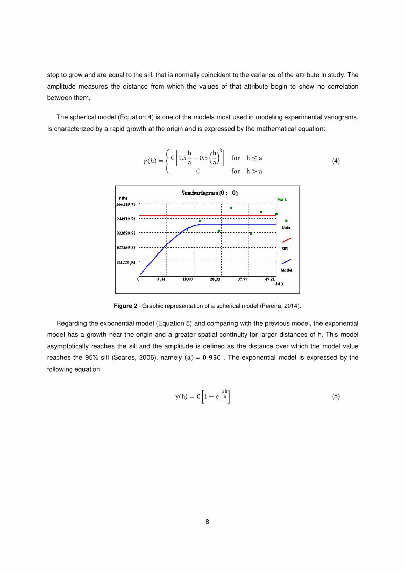
The spherical model (Equation 4) is one of the models most used in modeling experimental variograms.
Is characterized by a rapid growth at the origin and is expressed by the mathematical equation:
%(ℎ) = & C '1.5 ha − 0.5 *ha+,- for h ≤ aC for h > a (4)
Figure 2 - Graphic representation of a spherical model (Pereira, 2014).
Regarding the exponential model (Equation 5) and comparing with the previous model, the exponential
model has a growth near the origin and a greater spatial continuity for larger distances of h. This model
asymptotically reaches the sill and the amplitude is defined as the distance over which the model value
reaches the 95% sill (Soares, 2006), namely (3) = 4, 678 . The exponential model is expressed by the
following equation:
γ(h) = C 91 − e;,<= > (5)
9
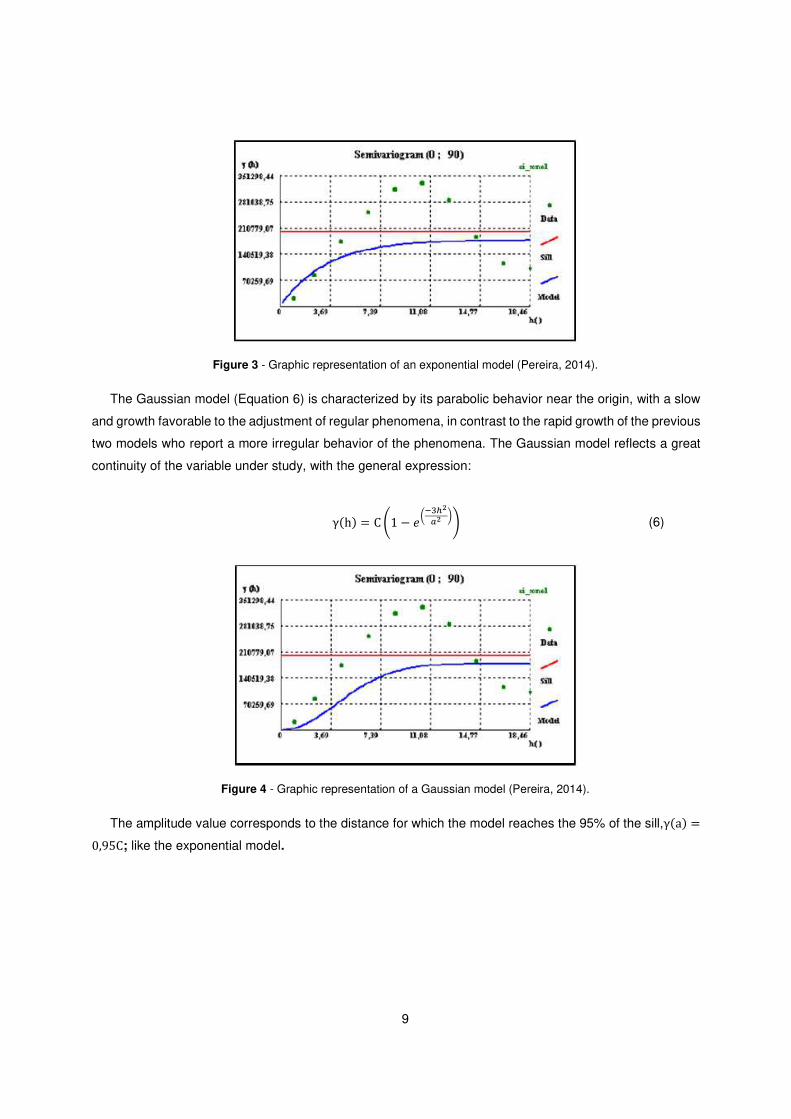
Figure 3 - Graphic representation of an exponential model (Pereira, 2014).
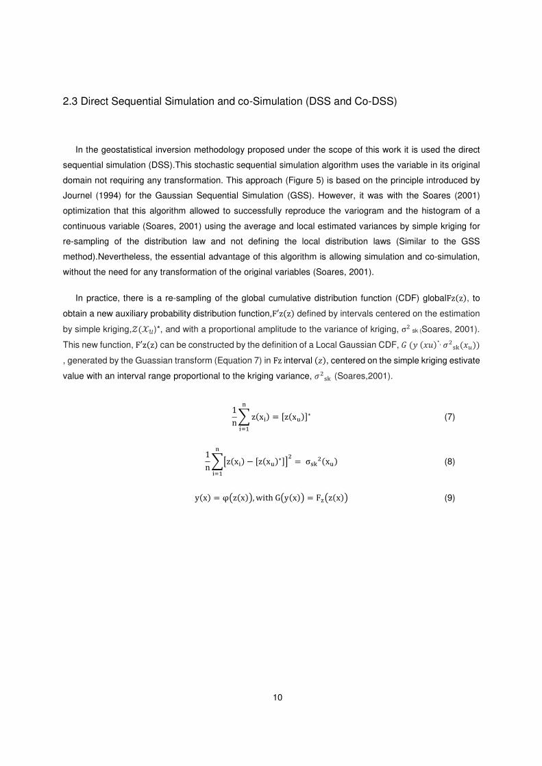
The Gaussian model (Equation 6) is characterized by its parabolic behavior near the origin, with a slow
and growth favorable to the adjustment of regular phenomena, in contrast to the rapid growth of the previous
two models who report a more irregular behavior of the phenomena. The Gaussian model reflects a great
continuity of the variable under study, with the general expression:
γ(h) = C ?1 − @*;,ABCB +D (6)
Figure 4 - Graphic representation of a Gaussian model (Pereira, 2014).
The amplitude value corresponds to the distance for which the model reaches the 95% of the sill,γ(a) =0,95C; like the exponential model.
10
2.3 Direct Sequential Simulation and co-Simulation (DSS and Co-DSS)
In the geostatistical inversion methodology proposed under the scope of this work it is used the direct
sequential simulation (DSS).This stochastic sequential simulation algorithm uses the variable in its original
domain not requiring any transformation. This approach (Figure 5) is based on the principle introduced by
Journel (1994) for the Gaussian Sequential Simulation (GSS). However, it was with the Soares (2001)
optimization that this algorithm allowed to successfully reproduce the variogram and the histogram of a
continuous variable (Soares, 2001) using the average and local estimated variances by simple kriging for
re-sampling of the distribution law and not defining the local distribution laws (Similar to the GSS
method).Nevertheless, the essential advantage of this algorithm is allowing simulation and co-simulation,
without the need for any transformation of the original variables (Soares, 2001).
In practice, there is a re-sampling of the global cumulative distribution function (CDF) globalFz(z), to
obtain a new auxiliary probability distribution function,F′z(z) defined by intervals centered on the estimation
by simple kriging,I(JK)*, and with a proportional amplitude to the variance of kriging, σ� sk (Soares, 2001).
This new function, F′z(z) can be constructed by the definition of a Local Gaussian CDF, � (� (��)*, ��MN(�O))
, generated by the Guassian transform (Equation 7) in Fz interval (P), centered on the simple kriging estivate
value with an interval range proportional to the kriging variance, ��MN (Soares,2001).
1n Q z(xR)S
RTU = [z(xV)]∗ (7)
1n QXz(xR) − [z(xV)∗]Y� = σMN�(xV)S
RTU (8)
y(x) = φ�z(x)�, with G�y(x)� = F`�z(x)� (9)
11
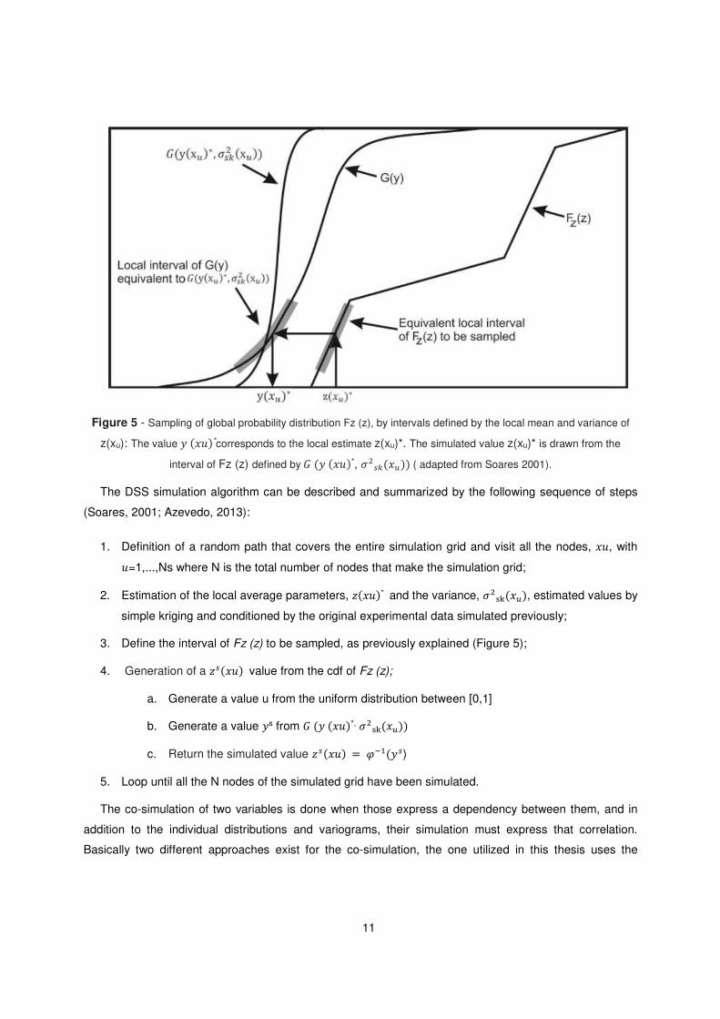
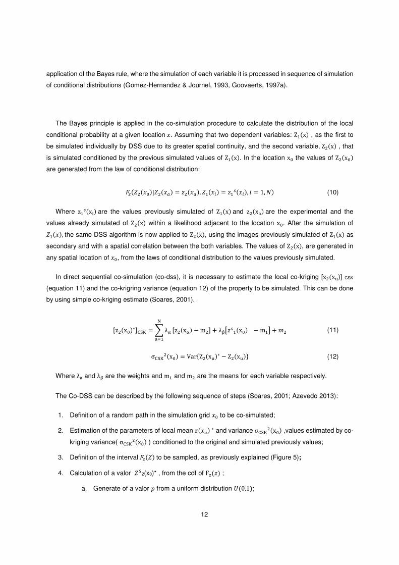
Figure 5 - Sampling of global probability distribution Fz (z), by intervals defined by the local mean and variance of
z(xu): The value � (��)*corresponds to the local estimate z(xu)*. The simulated value z(xu)* is drawn from the
interval of Fz (z) defined by � (� (��)*, ��ab(�O)) ( adapted from Soares 2001).
The DSS simulation algorithm can be described and summarized by the following sequence of steps
(Soares, 2001; Azevedo, 2013):
1. Definition of a random path that covers the entire simulation grid and visit all the nodes, ��, with �=1,...,Ns where N is the total number of nodes that make the simulation grid;
2. Estimation of the local average parameters, P(��)* and the variance, ��MN(�O), estimated values by
simple kriging and conditioned by the original experimental data simulated previously;
3. Define the interval of Fz (z) to be sampled, as previously explained (Figure 5);
4. Generation of a Pa(��) value from the cdf of Fz (z);
a. Generate a value u from the uniform distribution between [0,1]
b. Generate a value �s from � (� (��)*, ��MN(�O))
c. Return the simulated value Pa(��) = c;U(�a) 5. Loop until all the N nodes of the simulated grid have been simulated.
The co-simulation of two variables is done when those express a dependency between them, and in
addition to the individual distributions and variograms, their simulation must express that correlation.
Basically two different approaches exist for the co-simulation, the one utilized in this thesis uses the
12
application of the Bayes rule, where the simulation of each variable it is processed in sequence of simulation
of conditional distributions (Gomez-Hernandez & Journel, 1993, Goovaerts, 1997a).
The Bayes principle is applied in the co-simulation procedure to calculate the distribution of the local
conditional probability at a given location �. Assuming that two dependent variables: ZU(x) , as the first to
be simulated individually by DSS due to its greater spatial continuity, and the second variable, Z�(x) , that
is simulated conditioned by the previous simulated values of ZU(x). In the location xd the values of Z�(xd)
are generated from the law of conditional distribution:
ef(g�(�d)|g�(�C) = P�(�C), gU(�h) = PU a(�h), i = 1, j) (10)
Where zUM(xR) are the values previously simulated of ZU(x) and z�(x=) are the experimental and the
values already simulated of Z�(x) within a likelihood adjacent to the location xd. After the simulation of gU(�), the same DSS algorithm is now applied to Z�(x), using the images previously simulated of ZU(x) as
secondary and with a spatial correlation between the both variables. The values of Z�(x), are generated in
any spatial location of �d, from the laws of conditional distribution to the values previously simulated.
In direct sequential co-simulation (co-dss), it is necessary to estimate the local co-kriging [z�(xV)] CSK
(equation 11) and the co-krigring variance (equation 12) of the property to be simulated. This can be done
by using simple co-kriging estimate (Soares, 2001).
[z�(xd)∗]klm = Q λop
=TU[z�(xo) − m�] + λrXPaU(xd) − mUY + s� (11)
σklm�(xd) = Var�Z�(xV)∗ − Z�(xV) (12)
Where λ= and λr are the weights and mU and m� are the means for each variable respectively.
The Co-DSS can be described by the following sequence of steps (Soares, 2001; Azevedo 2013):
1. Definition of a random path in the simulation grid �d to be co-simulated;
2. Estimation of the parameters of local mean P(�O) ∗ and variance σklm�(xd) ,values estimated by co-
kriging variance( σklm�(xd) ) conditioned to the original and simulated previously values;
3. Definition of the interval ef(g) to be sampled, as previously explained (Figure 5);
4. Calculation of a valor gu2(x0)* , from the cdf of F`(P) ;
a. Generate of a valor v from a uniform distribution w(0,1);
13
b. Generate a valor �� from � (�(�d)*, σ�xMN(�d)) ;
c. Return the simulated value g� a(�d) = c;U(�a) 5. Loop until all the N nodes of the simulated grid have been simulated.
The co-simulated models allow to reproduction of the values of the experimental data ((P� (�C)) in their
locations, the marginal probability distribution of ef(P) and the pattern spatial continuity imposed by a
variogram model. However the simulated models that result from the co-DSS only allow the representation
of linear correlations between the primary and secondary variables, independently from the joint probability
distribution observed in the experimental data (Horta & Soares, 2010).
2.4. Direct Sequential co-simulation with joint probability distributions
Because of the limitations regarding the assumption of linear correlation between primary and secondary
variables, the traditional Co-DSS methodology, was modified to include non-linear correlations. This new
approximation, introduced by Horta & Soares (2010) and named direct co-simulation with joint probability
distributions ensures the reproduction of the experimental joint probability distribution between the primary
and secondary variables on the simulated models (Horta & Soares 2010).
As any stochastic sequential simulation, the procedure of the co-DSS with joint distributions is based in
the application of the Bayes principal, in a successive sequence of steps. This principle is in the base of the
estimation of the local conditional probability distributions, sequentially in every node of the simulation grid
(Azevedo, 2013). The simulation methodologies assume, in a model previously simulated, the secondary
variable,ZU(x) is initially calculated for all the simulation grid: followed by the primary variableZ�(x). The local
cumulative distribution function, from where the value of z�y (x) is calculated, is defined by the simple co-
located co-kriging estimate and by the co-kriging variance. When compared with the traditional co-DSS, the
main difference in this approximation is the way that the conditional cdf (F (Z�(x)|ZU(�)), is sampled. The
value of z�y (�), instead of being calculated from the global cumulative distribution function, like in the
traditional co-DSS, is calculated from the local conditional distribution, expressed by the next equation
(Equation 13) (Horta & Soares 2010):
F[Z�(u)|ZU(u) = ZU(u)∗] = prob�Z�(u) < z|ZU(u)∗ K (13)
The co-DSS algorithm with joint probability distributions, allows the reproduction of the values of the
experimental data in their locations in the simulated models, the original spatial continuity model and
reproduces the marginal distributions from the primary variable. This co-DSS algorithm distinguishes by the
14
ability to reproduce the joint distributions, estimated from the experimental data between the primary and
secondary variable,e (g�(�)|gU(�)) even when the original joint distribution is complex (Azevedo, 2013).
The procedure of the co-DSS algorithm can be synthetized by the following steps (Horta & Soares, 2010;
Azevedo, 2013)
1) Estimation of the global bi-distribution, e (g�(�)|gU(�)), from the experimental data;
2) Simulation of a secondary variable ZU(x), with the DSS algorithm for all the simulation grid;
3) Estimate the local mean and variance in, �O, with the estimation of the simple co-krigring co-
localized and correspondence co-krigring variance, conditioned by the original experimental data Z�(x=), by the data previously simulated Z�(x=)* end by the secondary variable value ZU(xV)*, inside
an adjacent likelihood u;
4) Calculation the cdf,F (Z�(x)|ZU(x)), with the simulated values of the secondary variable , PU�(u).
5) Simulation of the value P��(u) , from the conditional cdf, ,F (z�(x)|zU(x) = zUy(u)) , using the
approximation of the traditional DSS algorithm;
6) The models resulting of the stochastic simulation, from the co-DSS with joint probability distributions
application, ensure the spatial reproduction of the bi-distributions between the primary and the
secondary variables (Azevedo, 2013). With a representation of the vertical sections related with a
velocity model of P waves we can see the differences between the co-simulation of the models that
are the result of the DSS and the models that result from the use of DSS with joint probability
distributions and the last one, presents a bigger variability with a detailed approximation, compared
with the original co-DSS.
15
Chapter 3: Integration of Seismic data In Reservoir Modeling Characterization
3.1 Seismic inversion
Over the last few years, seismic inversion techniques had a major impact in the characterization of the
subsurface geology, helping the professionals to make better and more efficient decisions on the oil industry.
Seismic reflection data is used in reservoir characterization not only for obtaining a geometric description of
the main subsurface structures but also for estimating the spatial distribution of the subsurface properties
such as lithology and fluids. However, transforming seismic data into reservoir properties is an inverse
problem with a non-unique solution even for noise-free data, due to the limited frequency of recorded
seismic waves, forward-modeling simplifications needed to obtain solutions in a reasonable time,
uncertainties in well-to-seismic ties (depth-to-time conversion), in estimating a representative wavelet and
in the links between reservoir and elastic properties. (Bosch et al., 2010). The main objective of a study
associated with the use of seismic inversion techniques is the inference of the subsurface elastic properties
from available seismic reflection data. The process of predicting the behavior of a particular physical system
under investigation is normally designed as forward modelling. The relationship between the observed data
and the earth models can be express by the next equation (Tarantola, 2005; Azevedo et al., 2012):
���� = �(�) + � (14)
Considering the case of seismic inversion problems, ���a represents the recorded seismic reflection data,
F is the convolution model and m is the model parameter space for the properties to invert that depend on
the objective of the inversion, which can be acoustic impedance and/or elastic impedance, density or the P
and S wave velocities. The forward model (F) related to the previous equation can be defined by the next
equation:
� = � ∗ � (15)
where A corresponds to the recorded seismic amplitudes, r to the reflection coefficient of the subsurface
that are convolve with a wavelet w. Theses variables are dependent on the elastic properties ( density and
P and S wave velocities) of the subsurface geology ( Azevedo,2013).
Therefore the seismic method has some limitations that make the seismic inversion problems non-linear
and with multiple solutions, the limited bandwidth and resolution of the seismic reflection data, noise,
measurement errors, numerical approximations and physical assumptions about the involved forward
16
models (Tarantola 2005;Bosch et al. 2010; Tompkins et al. 2011). Because of these limitations, the inverted
elastic models, that are the result of the seismic inversion process, are only a possibility between n models
of the earth that are unknown, which equally satisfy the same observed seismic data (Azevedo, 2013), this
means that exist multiple acceptable solutions for the convolution of the reflection series with the wavelet
combined with the observed seismic (Francis, 2005). Therefore if the correlation between the recorded
seismic and the synthetic seismic, calculated from the best inverted models, is weak, then we can conclude
that the correlation between the correspondent real elastic and synthetic models will be weak too (Azevedo,
2013).
Inverted elastic Earth models are nowadays routinely used in reservoir characterization studies. Because
of this reason it is extremely important to understand the different seismic inverse methodologies and the
assumptions associated with each, assumptions about prior probability distributions and about spatial
continuity patterns have a significant impact in the exploration of the model parameter space and
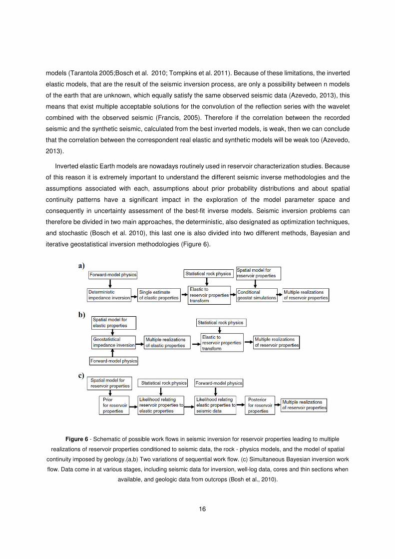
consequently in uncertainty assessment of the best-fit inverse models. Seismic inversion problems can
therefore be divided in two main approaches, the deterministic, also designated as optimization techniques,
and stochastic (Bosch et al. 2010), this last one is also divided into two different methods, Bayesian and
iterative geostatistical inversion methodologies (Figure 6).
Figure 6 - Schematic of possible work flows in seismic inversion for reservoir properties leading to multiple
realizations of reservoir properties conditioned to seismic data, the rock - physics models, and the model of spatial
continuity imposed by geology.(a,b) Two variations of sequential work flow. (c) Simultaneous Bayesian inversion work
flow. Data come in at various stages, including seismic data for inversion, well-log data, cores and thin sections when
available, and geologic data from outcrops (Bosh et al., 2010).
17
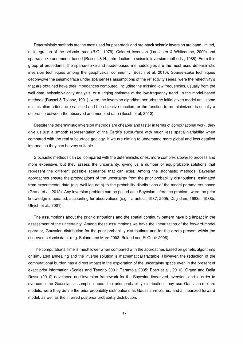
Deterministic methods are the most used for post-stack and pre-stack seismic inversion are band-limited,
or integration of the seismic trace (R.O., 1979), Colored Inversion (Lancaster & Whitcombe, 2000) and
sparse-spike and model-based (Russell & H., Introduction to seismic inversion methods , 1988). From this
group of procedures, the sparse-spike and model-based methodologies are the most used deterministic
inversion techniques among the geophysical community (Bosch et al, 2010). Sparse-spike techniques
deconvolve the seismic trace under sparseness assumptions of the reflectivity series, were the reflectivity’s
that are obtained have their impedances computed, including the missing low frequencies, usually from the
well data, seismic-velocity analysis, or a kriging estimate of the low-frequency trend. In the model-based
methods (Russel & Toksoz, 1991), were the inversion algorithm perturbs the initial given model until some
minimization criteria are satisfied and the objective function, or the function to be minimized, is usually a
difference between the observed and modeled data (Bosch et al, 2010).
Despite the deterministic inversion methods are cheaper and faster in terms of computational work, they
give us just a smooth representation of the Earth’s subsurface with much less spatial variability when
compared with the real subsurface geology. If we are aiming to understand more global and less detailed
information they can be very suitable.
Stochastic methods can be, compared with the deterministic ones, more complex slower to process and
more expensive, but they assess the uncertainty, giving us a number of equiprobable solutions that
represent the different possible scenarios that can exist. Among the stochastic methods, Bayesian
approaches ensure the propagations of the uncertainty from the prior probability distributions, estimated
from experimental data (e.g. well-log data) to the probability distributions of the model parameters space
(Grana et al. 2012). Any inversion problem can be posed as a Bayesian inference problem, were the prior
knowledge is updated, accounting for observations (e.g. Tarantola, 1987, 2005; Duijndam, 1988a, 1988b;
Ulrych et al., 2001).
The assumptions about the prior distributions and the spatial continuity pattern have big impact in the
assessment of the uncertainty. Among these assumptions we have the linearization of the forward-model
operator, Gaussian distribution for the prior probability distributions and for the errors present within the
observed seismic data. (e.g. Buland and More 2003; Buland and El Ouair 2006).
The computational time is much lower when compared with the approaches based on genetic algorithms
or simulated annealing and the inverse solution is mathematical tractable. However, the reduction of the
computational burden has a direct impact in the exploration of the uncertainty space even in the present of
exact prior information (Scales and Tenorio 2001; Tarantola 2005; Bosh et al., 2010). Grana and Della
Rossa (2010) developed and inversion framework for the Bayesian linearized inversion, and in order to
overcome the Gaussian assumption about the prior probability distribution, they use Gaussian-mixture
models, were they define the prior probability distributions as Gaussian-mixtures, and a linearized forward
model, as well as the inferred posterior probability distribution.
18
Geostatistical approaches define the inverse solution as a probability density function on the model
parameters space (Bosch et al., 2010). Normally the inverse solution is achieved by sampling the model
parameter space by Monte Carlo or by using geostatistical sequential simulation combined with global
optimization algorithms. Genetic algorithms (e.g. Mallic 1995; Mallick 1999; Boschetti, Dentith, and List1996;
Soares et al., 2007) and simulated annealing (Sen and Stoffa 1991; Ma 2002) fall within this class of inverse
methodologies.
3.2 Geostatistical Seismic Inversion
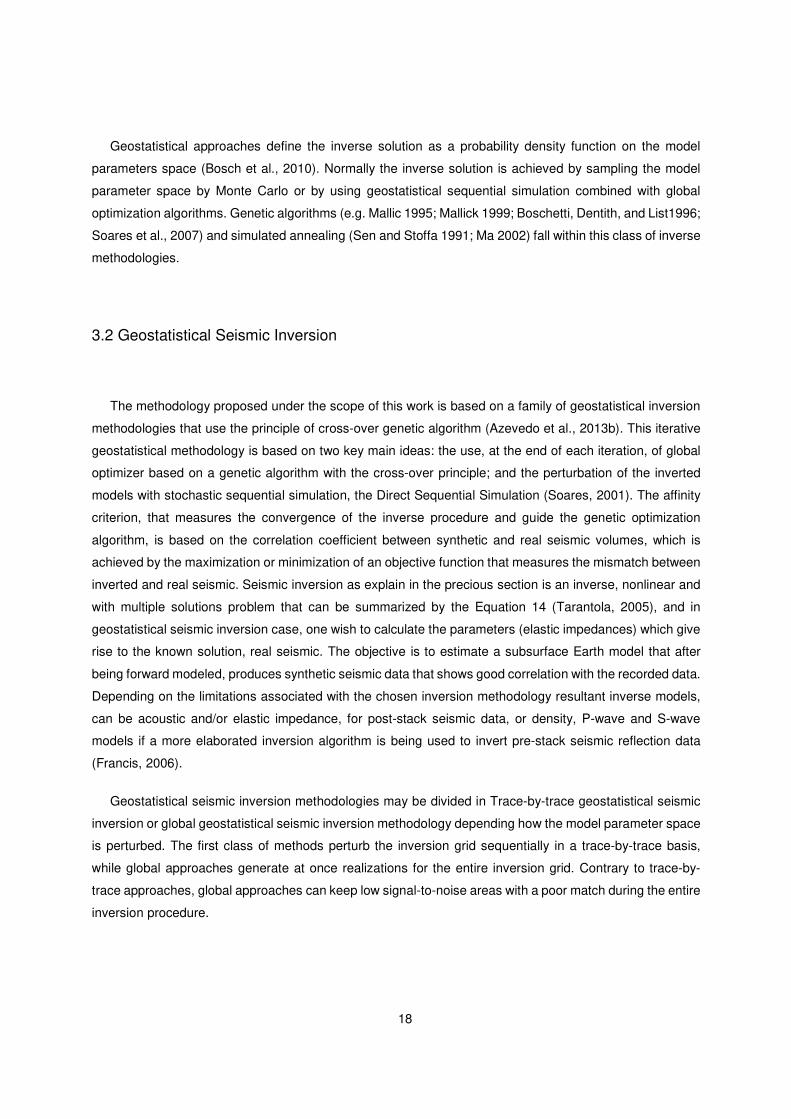
The methodology proposed under the scope of this work is based on a family of geostatistical inversion
methodologies that use the principle of cross-over genetic algorithm (Azevedo et al., 2013b). This iterative
geostatistical methodology is based on two key main ideas: the use, at the end of each iteration, of global
optimizer based on a genetic algorithm with the cross-over principle; and the perturbation of the inverted
models with stochastic sequential simulation, the Direct Sequential Simulation (Soares, 2001). The affinity
criterion, that measures the convergence of the inverse procedure and guide the genetic optimization
algorithm, is based on the correlation coefficient between synthetic and real seismic volumes, which is
achieved by the maximization or minimization of an objective function that measures the mismatch between
inverted and real seismic. Seismic inversion as explain in the precious section is an inverse, nonlinear and
with multiple solutions problem that can be summarized by the Equation 14 (Tarantola, 2005), and in
geostatistical seismic inversion case, one wish to calculate the parameters (elastic impedances) which give
rise to the known solution, real seismic. The objective is to estimate a subsurface Earth model that after
being forward modeled, produces synthetic seismic data that shows good correlation with the recorded data.
Depending on the limitations associated with the chosen inversion methodology resultant inverse models,
can be acoustic and/or elastic impedance, for post-stack seismic data, or density, P-wave and S-wave
models if a more elaborated inversion algorithm is being used to invert pre-stack seismic reflection data
(Francis, 2006).
Geostatistical seismic inversion methodologies may be divided in Trace-by-trace geostatistical seismic
inversion or global geostatistical seismic inversion methodology depending how the model parameter space
is perturbed. The first class of methods perturb the inversion grid sequentially in a trace-by-trace basis,
while global approaches generate at once realizations for the entire inversion grid. Contrary to trace-by-
trace approaches, global approaches can keep low signal-to-noise areas with a poor match during the entire
inversion procedure.
19
3.3 Time-Lapse Seismic
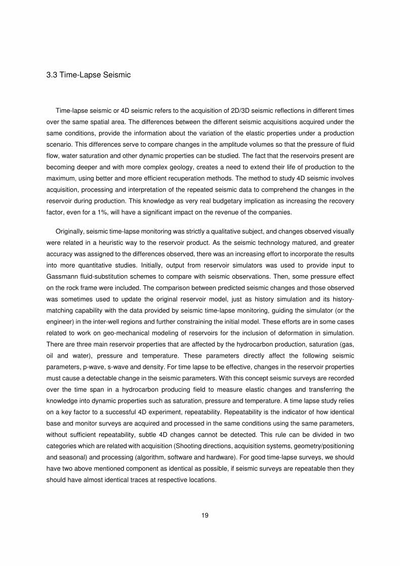
Time-lapse seismic or 4D seismic refers to the acquisition of 2D/3D seismic reflections in different times
over the same spatial area. The differences between the different seismic acquisitions acquired under the
same conditions, provide the information about the variation of the elastic properties under a production
scenario. This differences serve to compare changes in the amplitude volumes so that the pressure of fluid
flow, water saturation and other dynamic properties can be studied. The fact that the reservoirs present are
becoming deeper and with more complex geology, creates a need to extend their life of production to the
maximum, using better and more efficient recuperation methods. The method to study 4D seismic involves
acquisition, processing and interpretation of the repeated seismic data to comprehend the changes in the
reservoir during production. This knowledge as very real budgetary implication as increasing the recovery
factor, even for a 1%, will have a significant impact on the revenue of the companies.
Originally, seismic time-lapse monitoring was strictly a qualitative subject, and changes observed visually
were related in a heuristic way to the reservoir product. As the seismic technology matured, and greater
accuracy was assigned to the differences observed, there was an increasing effort to incorporate the results
into more quantitative studies. Initially, output from reservoir simulators was used to provide input to
Gassmann fluid-substitution schemes to compare with seismic observations. Then, some pressure effect
on the rock frame were included. The comparison between predicted seismic changes and those observed
was sometimes used to update the original reservoir model, just as history simulation and its history-
matching capability with the data provided by seismic time-lapse monitoring, guiding the simulator (or the
engineer) in the inter-well regions and further constraining the initial model. These efforts are in some cases
related to work on geo-mechanical modeling of reservoirs for the inclusion of deformation in simulation.
There are three main reservoir properties that are affected by the hydrocarbon production, saturation (gas,
oil and water), pressure and temperature. These parameters directly affect the following seismic
parameters, p-wave, s-wave and density. For time lapse to be effective, changes in the reservoir properties
must cause a detectable change in the seismic parameters. With this concept seismic surveys are recorded
over the time span in a hydrocarbon producing field to measure elastic changes and transferring the
knowledge into dynamic properties such as saturation, pressure and temperature. A time lapse study relies
on a key factor to a successful 4D experiment, repeatability. Repeatability is the indicator of how identical
base and monitor surveys are acquired and processed in the same conditions using the same parameters,
without sufficient repeatability, subtle 4D changes cannot be detected. This rule can be divided in two
categories which are related with acquisition (Shooting directions, acquisition systems, geometry/positioning
and seasonal) and processing (algorithm, software and hardware). For good time-lapse surveys, we should
have two above mentioned component as identical as possible, if seismic surveys are repeatable then they
should have almost identical traces at respective locations.
20
Observations made on seismic time-lapse studies frequently include changes in amplitude and changes
in time. Changes in amplitude can often be used to directly monitor fluid migration because the reflection
character changes by replacing oil/water with gas for example. Other changes in reservoir properties must
always be considered, such as effective pressure acting on the rock frame, and it is not always possible to
separate these effects using stacked data alone. The use of offset stacks or elastic impedance volumes
helps to reduce this uncertainty, separating the changes that seem to be caused by fluid substitution from
those caused by pressure change, and a seismic petro-physical model in required in the interpretation. The
change in seismic velocity between separate monitoring experiments will also result in a change of two-way
travel time to reflectors that lie beneath the producing reservoir. This velocity-induced “pull-up” may be
monitored and provides an indication of the spatial location of reservoir changes. Because of this effect,
interpreters should take great care in the use of direct difference volumes that are obtained simple by
subtraction of seismic volumes obtained at different times, the seismic reflection data should be processed
in order to address this problems.
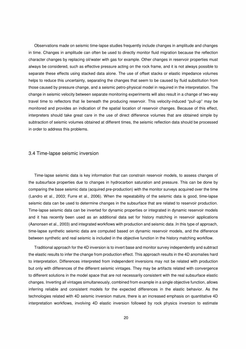
3.4 Time-lapse seismic inversion
Time-lapse seismic data is key information that can constrain reservoir models, to assess changes of
the subsurface properties due to changes in hydrocarbon saturation and pressure. This can be done by
comparing the base seismic data (acquired pre-production) with the monitor surveys acquired over the time
(Landro et al., 2003; Furre et al., 2006). When the repeatability of the seismic data is good, time-lapse
seismic data can be used to determine changes in the subsurface that are related to reservoir production.
Time-lapse seismic data can be inverted for dynamic properties or integrated in dynamic reservoir models
and it has recently been used as an additional data set for history matching in reservoir applications
(Aanonsen et al., 2003) and integrated workflows with production and seismic data .In this type of approach,
time-lapse synthetic seismic data are computed based on dynamic reservoir models, and the difference
between synthetic and real seismic is included in the objective function in the history matching workflow.
Traditional approach for the 4D inversion is to invert base and monitor survey independently and subtract
the elastic results to infer the change from production effect. This approach results in the 4D anomalies hard
to interpretation. Differences interpreted from independent inversions may not be related with production
but only with differences of the different seismic vintages. They may be artifacts related with convergence
to different solutions in the model space that are not necessarily consistent with the real subsurface elastic
changes. Inverting all vintages simultaneously, combined from example in a single objective function, allows
inferring reliable and consistent models for the expected differences in the elastic behavior. As the
technologies related with 4D seismic inversion mature, there is an increased emphasis on quantitative 4D
interpretation workflows, involving 4D elastic inversion followed by rock physics inversion to estimate
21
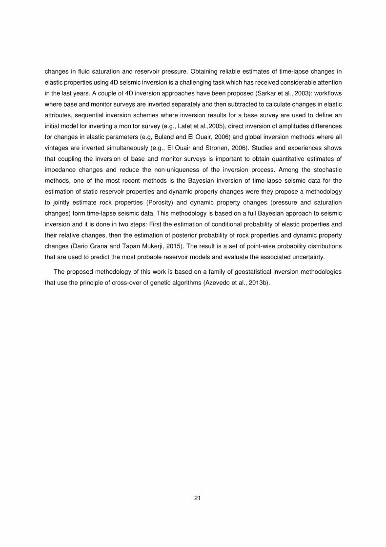
changes in fluid saturation and reservoir pressure. Obtaining reliable estimates of time-lapse changes in
elastic properties using 4D seismic inversion is a challenging task which has received considerable attention
in the last years. A couple of 4D inversion approaches have been proposed (Sarkar et al., 2003): workflows
where base and monitor surveys are inverted separately and then subtracted to calculate changes in elastic
attributes, sequential inversion schemes where inversion results for a base survey are used to define an
initial model for inverting a monitor survey (e.g., Lafet et al.,2005), direct inversion of amplitudes differences
for changes in elastic parameters (e.g, Buland and El Ouair, 2006) and global inversion methods where all
vintages are inverted simultaneously (e.g., El Ouair and Stronen, 2006). Studies and experiences shows
that coupling the inversion of base and monitor surveys is important to obtain quantitative estimates of
impedance changes and reduce the non-uniqueness of the inversion process. Among the stochastic
methods, one of the most recent methods is the Bayesian inversion of time-lapse seismic data for the
estimation of static reservoir properties and dynamic property changes were they propose a methodology
to jointly estimate rock properties (Porosity) and dynamic property changes (pressure and saturation
changes) form time-lapse seismic data. This methodology is based on a full Bayesian approach to seismic
inversion and it is done in two steps: First the estimation of conditional probability of elastic properties and
their relative changes, then the estimation of posterior probability of rock properties and dynamic property
changes (Dario Grana and Tapan Mukerji, 2015). The result is a set of point-wise probability distributions
that are used to predict the most probable reservoir models and evaluate the associated uncertainty.
The proposed methodology of this work is based on a family of geostatistical inversion methodologies
that use the principle of cross-over of genetic algorithms (Azevedo et al., 2013b).

22
23
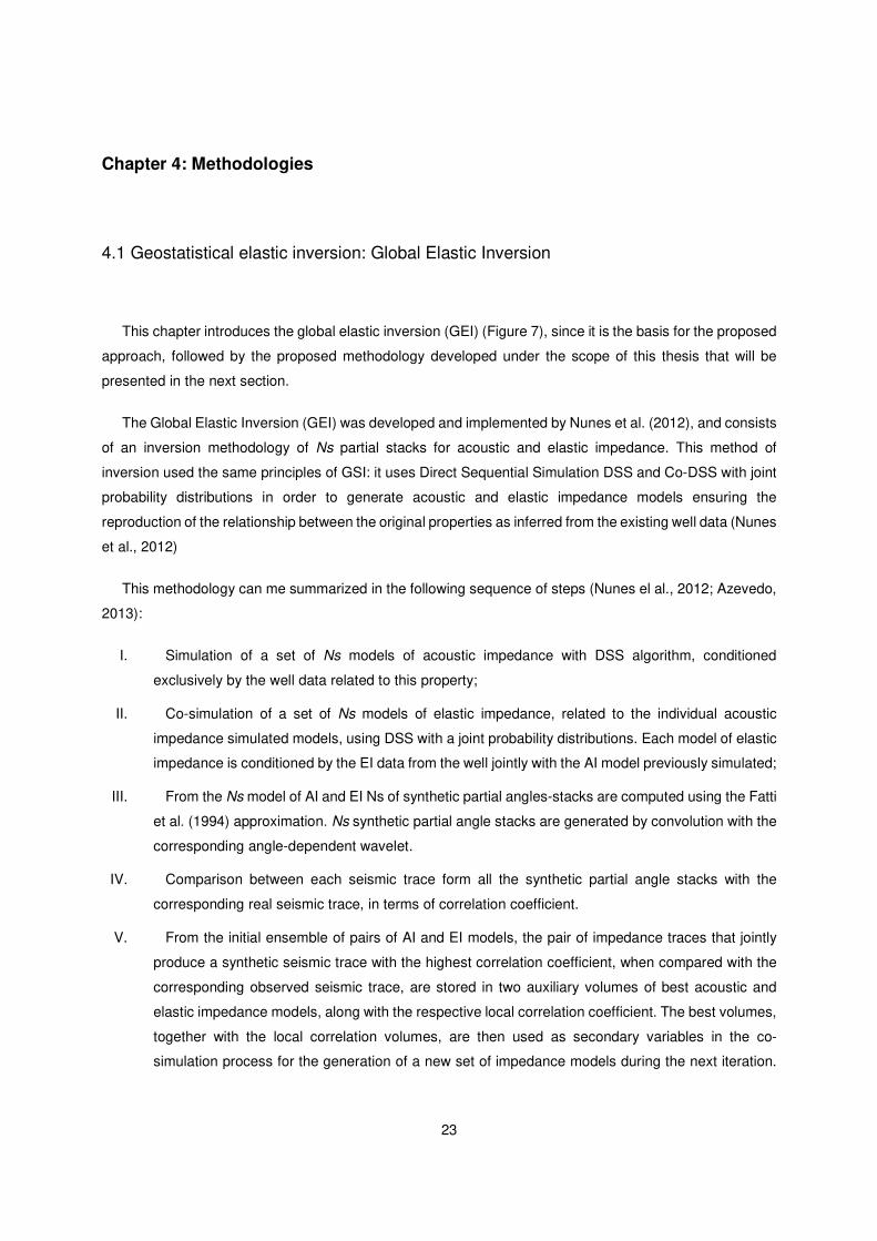
Chapter 4: Methodologies
4.1 Geostatistical elastic inversion: Global Elastic Inversion
This chapter introduces the global elastic inversion (GEI) (Figure 7), since it is the basis for the proposed
approach, followed by the proposed methodology developed under the scope of this thesis that will be
presented in the next section.
The Global Elastic Inversion (GEI) was developed and implemented by Nunes et al. (2012), and consists
of an inversion methodology of Ns partial stacks for acoustic and elastic impedance. This method of
inversion used the same principles of GSI: it uses Direct Sequential Simulation DSS and Co-DSS with joint
probability distributions in order to generate acoustic and elastic impedance models ensuring the
reproduction of the relationship between the original properties as inferred from the existing well data (Nunes
et al., 2012)
This methodology can me summarized in the following sequence of steps (Nunes el al., 2012; Azevedo,
2013):
I. Simulation of a set of Ns models of acoustic impedance with DSS algorithm, conditioned
exclusively by the well data related to this property;
II. Co-simulation of a set of Ns models of elastic impedance, related to the individual acoustic
impedance simulated models, using DSS with a joint probability distributions. Each model of elastic
impedance is conditioned by the EI data from the well jointly with the AI model previously simulated;
III. From the Ns model of AI and EI Ns of synthetic partial angles-stacks are computed using the Fatti
et al. (1994) approximation. Ns synthetic partial angle stacks are generated by convolution with the
corresponding angle-dependent wavelet.
IV. Comparison between each seismic trace form all the synthetic partial angle stacks with the
corresponding real seismic trace, in terms of correlation coefficient.
V. From the initial ensemble of pairs of AI and EI models, the pair of impedance traces that jointly
produce a synthetic seismic trace with the highest correlation coefficient, when compared with the
corresponding observed seismic trace, are stored in two auxiliary volumes of best acoustic and
elastic impedance models, along with the respective local correlation coefficient. The best volumes,
together with the local correlation volumes, are then used as secondary variables in the co-
simulation process for the generation of a new set of impedance models during the next iteration.
24
After iteration one the ensemble of AI models is simulated conditioned to the available acoustic
impedance well-log data, the best AI and the local correlation volumes from the previous iteration.
In the same way EI models generated after iteration one, are co-simulated using previously
simulated AI model, as auxiliary model, conditioned to the available elastic impedance well-log data
and the best EI and local correlation volumes from the previous iteration.
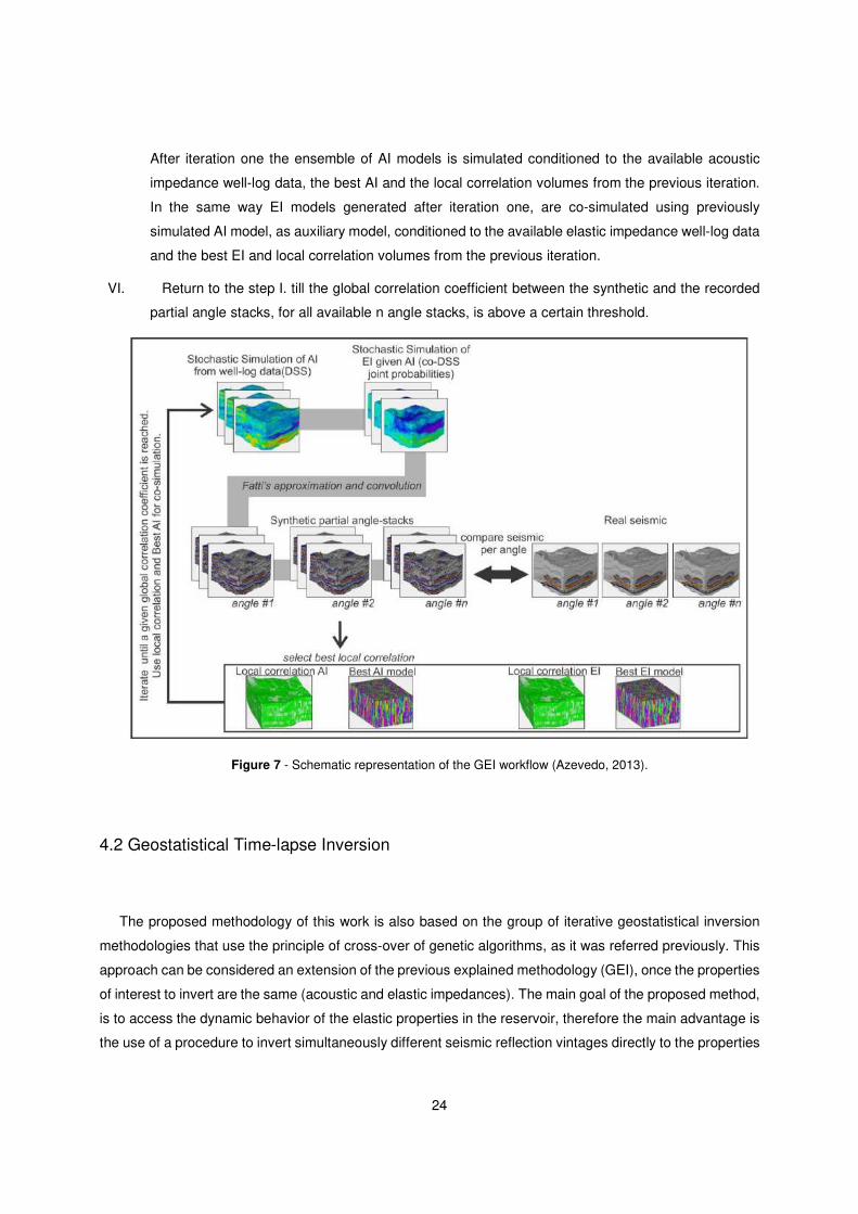
VI. Return to the step I. till the global correlation coefficient between the synthetic and the recorded
partial angle stacks, for all available n angle stacks, is above a certain threshold.
Figure 7 - Schematic representation of the GEI workflow (Azevedo, 2013).
4.2 Geostatistical Time-lapse Inversion
The proposed methodology of this work is also based on the group of iterative geostatistical inversion
methodologies that use the principle of cross-over of genetic algorithms, as it was referred previously. This
approach can be considered an extension of the previous explained methodology (GEI), once the properties
of interest to invert are the same (acoustic and elastic impedances). The main goal of the proposed method,
is to access the dynamic behavior of the elastic properties in the reservoir, therefore the main advantage is
the use of a procedure to invert simultaneously different seismic reflection vintages directly to the properties

25
elastic differences. Due to this reason, we need to deal with the elastic changes that will correspond to our
hard data, traduced by the computation between the differences of the properties, associated to each
acquisition time during the production of the reservoir. The final inverted models are constituted by the
residuals representing a set of equiprobable scenarios of the elastic response that may allow us to access
and quantify the spatial uncertainty associated. Once the elastic changes are not verified in all the study
area as we can see through the seismic differences illustrated in Figure 1, it were used masks within the
inversion grid, in order to simulate exclusively in the elastic changes areas, avoiding the simulation of
residual values in zones where the changes were not noticed.
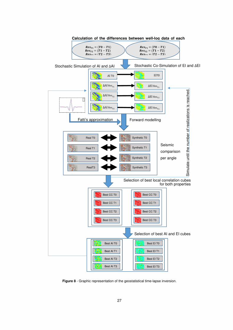
The general workflow of the proposed methodology is represented in the Figure 8 and it can be briefly
described by the following sequence of steps:
1) Calculate from the existing hard-data differences between well-log measurements related to each
different seismic vintage for each property to invert. These data will be used as conditioning in the
simulation procedure;
2) Stochastic sequential simulation of a set of Ns acoustic and elastic impedance models using DSS
and co-DSS with joint probability distributions respectively. Both properties are conditioned to the
available well log data and, in the case of elastic impedance, will also be conditioned to the previous
acoustic impedance model. For the acquisition time (T0) corresponding to the beginning of the
production, the well log data used are the original values of the elastic properties, once there are
no historic in elastic changes. To note that, the residues of each time are simulated in a masked
grid, conditioned by the differences between the seismic of each year: the zones which don’t occur
amplitude changes in the seismic data, are not simulated and are filled with the data from the
acoustic and elastic impedance models from the first year, in order to have the full grid to calculate
the synthetic seismic data.;
3) After the sum between the pair of the initial inverted models (T0) and the residuals from each time
of production (T10, T25 and T30), calculate synthetic seismic data volumes for those pairs of
realizations of each time generated in the previous step. The synthetic seismic data is obtained by
the convolution between the angle-dependent wavelets and the reflectivity coefficients computed
by Fatti´s approximation for each angle gather;
4) Compare the synthetic seismic volumes, in a trace-by-trace basis, with the corresponding
recorded seismic data in terms of correlation coefficient where the final result will be a best local
correlation cube that store the traces that produced the highest correlation coefficient. This process
of seismic comparison is applied to all times simultaneously obtaining, at the end of each iteration,
eight local correlation cubes: four volumes to each properties, each pair associated to each
acquisition time. From the best traces selected simultaneously and stored in the best correlation
coefficient volumes it will be computed the correspondent best elastic volumes for acoustic and

26
elastic impedances residuals. The best elastic residuals volumes along with the local correlation
coefficient volumes, after being subtracted by the T0 properties models, are used as secondary
variables in the co-simulation process for generating a new set of impedance residual models in the
next iteration. The new ensemble of impedance residual models, for the next iterations, will be
conditioned by the available well-log data (and each impedance model at each realization, in the
elastic case) but also by the best volumes (best elastic and local correlation cubes) computed in
the previous iteration. The iterative geostatistical inversion procedure finishes when global
correlation coefficient between the synthetic average and the recorded partial angle stacks, for all
the available n angle stacks, is above a certain threshold;
27
Figure 8 - Graphic representation of the geostatistical time-lapse inversion.
0 5 10 15 20 25 30 35-6
-4
-2
0
2
4
6
8
10x 10
5
0º
10º
20º
30º
40º
����� = (�4 − ��) ����� = (�� − ��) ����� = (�� − ��) ����� = (�4 − ��) ����� = (�� − ��) ����� = (�� − ��)
AI T0 EIT0
∆AI ResT1 ∆AI ResT2
∆AI ResT3
∆EI ResT1
∆EI ResT2
∆EI ResT3
Real T0 Synthetic T0
Synthetic T1
Synthetic T2
Synthetic T3
Real T1
Real T2
RealT3
Best CC T1
Best CC T0
Best CC T2
Best CC T3
Best CC T1
Best CC T0
Best CC T2
Best CC T3
Best AI T0
Best AI T1
Best AI T2
Best AI T3
Best EI T0
Best EI T1
Best EI T2
Best EI T3
Calculation of the differences between well-log data of each
Stochastic Simulation of AI and ∆AI Stochastic Co-Simulation of EI and ∆EI
Fatti’s approximation Forward modelling
Seismic
comparison
per angle
Sim
ula
te u
ntil th
e n
um
be
r o
f re
aliz
ation
s is r
ea
ch
ed.
Selection of best local correlation cubes for both properties
Selection of best AI and EI cubes

28
29
Chapter 5: Case Study
5.1 Data Description
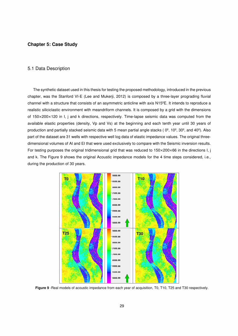
The synthetic dataset used in this thesis for testing the proposed methodology, introduced in the previous
chapter, was the Stanford VI-E (Lee and Mukerji, 2012) is composed by a three-layer prograding fluvial
channel with a structure that consists of an asymmetric anticline with axis N15ºE. It intends to reproduce a
realistic siliciclastic environment with meandriform channels. It is composed by a grid with the dimensions
of 150×200×120 in I, j and k directions, respectively. Time-lapse seismic data was computed from the
available elastic properties (density, Vp and Vs) at the beginning and each tenth year until 30 years of
production and partially stacked seismic data with 5 mean partial angle stacks ( 0º, 10º, 30º, and 40º). Also
part of the dataset are 31 wells with respective well log data of elastic impedance values. The original three-
dimensional volumes of AI and EI that were used exclusively to compare with the Seismic inversion results.
For testing purposes the original tridimensional grid that was reduced to 150×200×66 in the directions I, j
and k. The Figure 9 shows the original Acoustic impedance models for the 4 time steps considered, i.e.,
during the production of 30 years.
Figure 9 -Real models of acoustic impedance from each year of acquisition, T0, T10, T25 and T30 respectively.
T0
T30
T10
T25
30
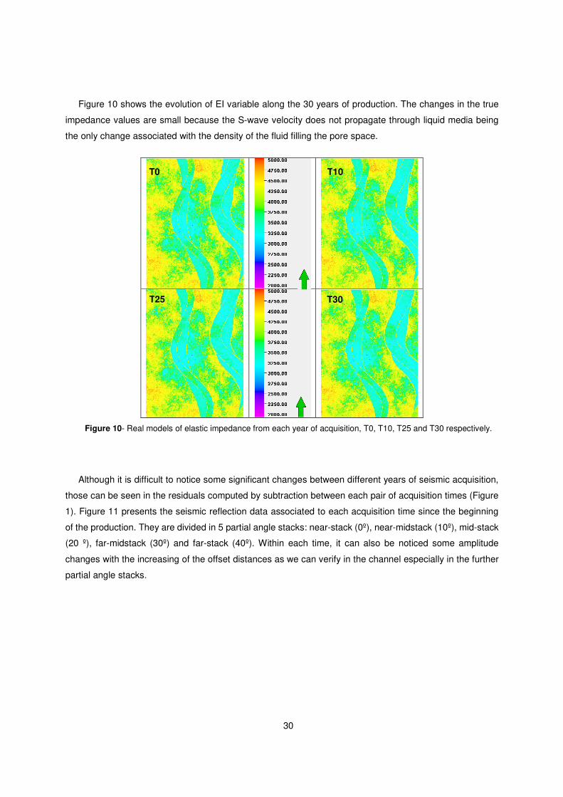
Figure 10 shows the evolution of EI variable along the 30 years of production. The changes in the true
impedance values are small because the S-wave velocity does not propagate through liquid media being
the only change associated with the density of the fluid filling the pore space.
Figure 10- Real models of elastic impedance from each year of acquisition, T0, T10, T25 and T30 respectively.
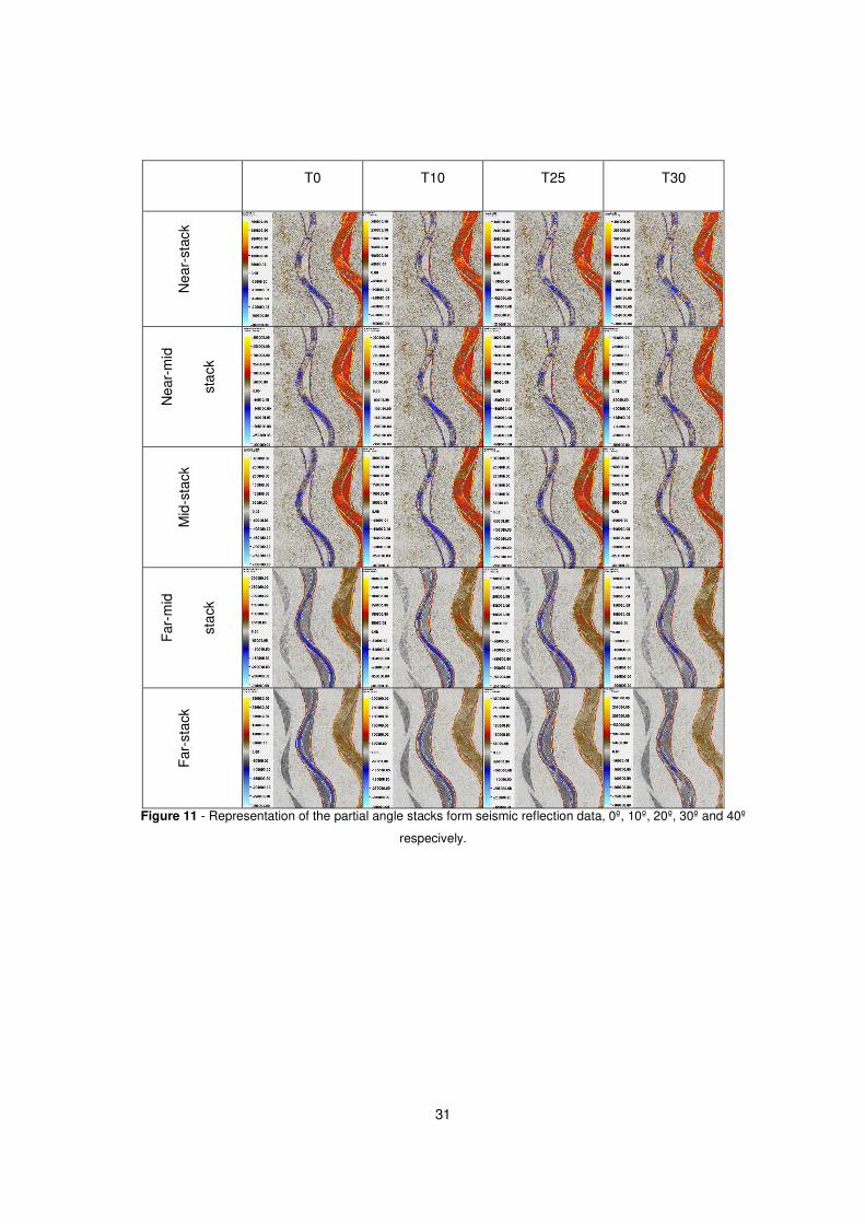
Although it is difficult to notice some significant changes between different years of seismic acquisition,
those can be seen in the residuals computed by subtraction between each pair of acquisition times (Figure
1). Figure 11 presents the seismic reflection data associated to each acquisition time since the beginning
of the production. They are divided in 5 partial angle stacks: near-stack (0º), near-midstack (10º), mid-stack
(20 º), far-midstack (30º) and far-stack (40º). Within each time, it can also be noticed some amplitude
changes with the increasing of the offset distances as we can verify in the channel especially in the further
partial angle stacks.
T0 T10
T25 T30
31
Figure 11 - Representation of the partial angle stacks form seismic reflection data, 0º, 10º, 20º, 30º and 40º
respecively.
T0 T10 T25 T30 N
ea
r-sta
ck
Ne
ar-
mid
sta
ck
Mid
-sta
ck
Fa
r-m
id
sta
ck
Fa
r-sta
ck
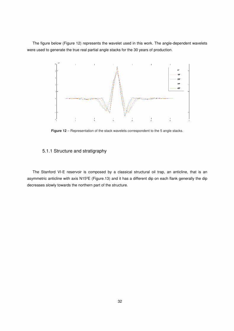
32
The figure below (Figure 12) represents the wavelet used in this work. The angle-dependent wavelets
were used to generate the true real partial angle stacks for the 30 years of production.
Figure 12 – Representation of the stack wavelets correspondent to the 5 angle stacks.
5.1.1 Structure and stratigraphy
The Stanford VI-E reservoir is composed by a classical structural oil trap, an anticline, that is an
asymmetric anticline with axis N15ºE (Figure.13) and it has a different dip on each flank generally the dip
decreases slowly towards the northern part of the structure.
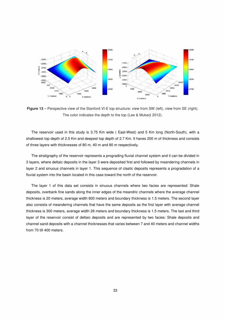
33
Figure 13 – Perspective view of the Stanford VI-E top structure: view from SW (left), view from SE (right).
The color indicates the depth to the top (Lee & Mukerji 2012).
The reservoir used in this study is 3.75 Km wide ( East-West) and 5 Km long (North-South), with a
shallowest top depth of 2.5 Km and deepest top depth of 2.7 Km. It haves 200 m of thickness and consists
of three layers with thicknesses of 80 m, 40 m and 80 m respectively.
The stratigraphy of the reservoir represents a prograding fluvial channel system and it can be divided in
3 layers, where deltaic deposits in the layer 3 were deposited first and followed by meandering channels in
layer 2 and sinuous channels in layer 1. This sequence of clastic deposits represents a progradation of a
fluvial system into the basin located in this case toward the north of the reservoir.
The layer 1 of this data set consists in sinuous channels where two facies are represented: Shale
deposits, overbank fine sands along the inner edges of the meandric channels where the average channel
thickness is 20 meters, average width 600 meters and boundary thickness is 1.5 meters. The second layer
also consists of meandering channels that have the same deposits as the first layer with average channel
thickness is 300 meters, average width 26 meters and boundary thickness is 1.5 meters. The last and third
layer of the reservoir consist of deltaic deposits and are represented by two facies: Shale deposits and
channel sand deposits with a channel thicknesses that varies between 7 and 40 meters and channel widths
from 70 till 400 meters.
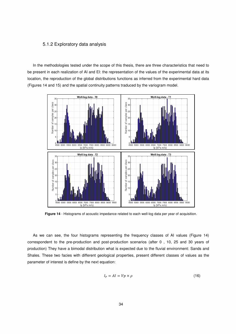
34
5.1.2 Exploratory data analysis
In the methodologies tested under the scope of this thesis, there are three characteristics that need to
be present in each realization of AI and EI: the representation of the values of the experimental data at its
location, the reproduction of the global distributions functions as inferred from the experimental hard data
(Figures 14 and 15) and the spatial continuity patterns traduced by the variogram model.
Figure 14 - Histograms of acoustic impedance related to each well-log data per year of acquisition.
As we can see, the four histograms representing the frequency classes of AI values (Figure 14)
correspondent to the pre-production and post-production scenarios (after 0 , 10, 25 and 30 years of
production) They have a bimodal distribution what is expected due to the fluvial environment: Sands and
Shales. These two facies with different geological properties, present different classes of values as the
parameter of interest is define by the next equation:
�� = �� = �v × (16)
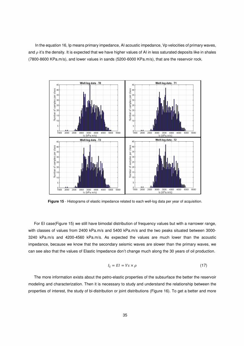
35
In the equation 16, Ip means primary impedance, AI acoustic impedance, Vp velocities of primary waves,
and it’s the density. It is expected that we have higher values of AI in less saturated deposits like in shales
(7800-8600 KPa.m/s), and lower values in sands (5200-6000 KPa.m/s), that are the reservoir rock.
Figure 15 - Histograms of elastic impedance related to each well-log data per year of acquisition.
For EI case(Figure 15) we still have bimodal distribution of frequency values but with a narrower range,
with classes of values from 2400 kPa.m/s and 5400 kPa.m/s and the two peaks situated between 3000-
3240 kPa.m/s and 4200-4560 kPa.m/s. As expected the values are much lower than the acoustic
impedance, because we know that the secondary seismic waves are slower than the primary waves, we
can see also that the values of Elastic Impedance don’t change much along the 30 years of oil production.
�u = ¡� = � × (17)
The more information exists about the petro-elastic properties of the subsurface the better the reservoir
modeling and characterization. Then it is necessary to study and understand the relationship between the
properties of interest, the study of bi-distribution or joint distributions (Figure 16). To get a better and more
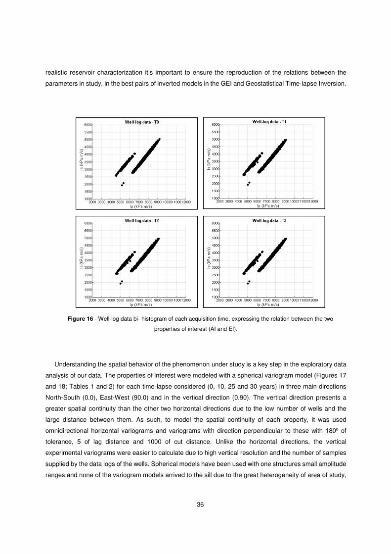
36
realistic reservoir characterization it’s important to ensure the reproduction of the relations between the
parameters in study, in the best pairs of inverted models in the GEI and Geostatistical Time-lapse Inversion.
Figure 16 - Well-log data bi- histogram of each acquisition time, expressing the relation between the two
properties of interest (AI and EI).
Understanding the spatial behavior of the phenomenon under study is a key step in the exploratory data
analysis of our data. The properties of interest were modeled with a spherical variogram model (Figures 17
and 18; Tables 1 and 2) for each time-lapse considered (0, 10, 25 and 30 years) in three main directions
North-South (0.0), East-West (90.0) and in the vertical direction (0.90). The vertical direction presents a
greater spatial continuity than the other two horizontal directions due to the low number of wells and the
large distance between them. As such, to model the spatial continuity of each property, it was used
omnidirectional horizontal variograms and variograms with direction perpendicular to these with 180º of
tolerance, 5 of lag distance and 1000 of cut distance. Unlike the horizontal directions, the vertical
experimental variograms were easier to calculate due to high vertical resolution and the number of samples
supplied by the data logs of the wells. Spherical models have been used with one structures small amplitude
ranges and none of the variogram models arrived to the sill due to the great heterogeneity of area of study,
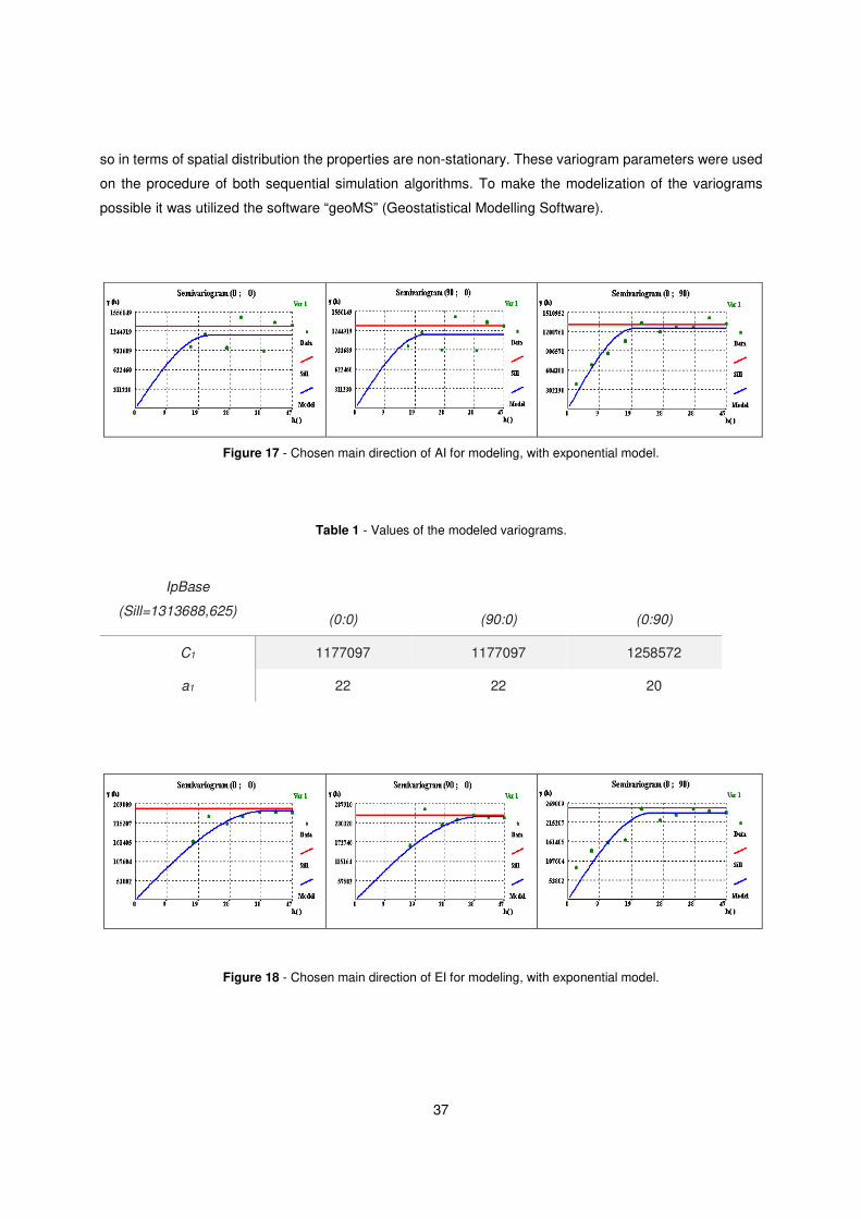
37
so in terms of spatial distribution the properties are non-stationary. These variogram parameters were used
on the procedure of both sequential simulation algorithms. To make the modelization of the variograms
possible it was utilized the software “geoMS” (Geostatistical Modelling Software).
Figure 17 - Chosen main direction of AI for modeling, with exponential model.
Table 1 - Values of the modeled variograms.
Figure 18 - Chosen main direction of EI for modeling, with exponential model.
IpBase
(Sill=1313688,625)
(0:0)
(90:0)
(0:90)
C1 1177097 1177097 1258572
a1 22 22 20
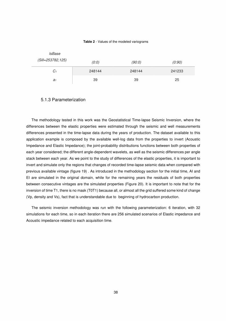
38
Table 2 - Values of the modeled variograms
IsBase
(Sill=253782,125)
(0:0)
(90:0)
(0:90)
C1 248144 248144 241233
a1 39 39 25
5.1.3 Parameterization
The methodology tested in this work was the Geostatistical Time-lapse Seismic Inversion, where the
differences between the elastic properties were estimated through the seismic and well measurements
differences presented in the time-lapse data during the years of production. The dataset available to this
application example is composed by the available well-log data from the properties to invert (Acoustic
Impedance and Elastic Impedance); the joint-probability distributions functions between both properties of
each year considered; the different angle-dependent wavelets, as well as the seismic differences per angle
stack between each year. As we point to the study of differences of the elastic properties, it is important to
invert and simulate only the regions that changes of recorded time-lapse seismic data when compared with
previous available vintage (figure 19) . As introduced in the methodology section for the initial time, AI and
EI are simulated in the original domain, while for the remaining years the residuals of both properties
between consecutive vintages are the simulated properties (Figure 20). It is important to note that for the
inversion of time T1, there is no mask (T0T1) because all, or almost all the grid suffered some kind of change
(Vp, density and Vs), fact that is understandable due to beginning of hydrocarbon production.
The seismic inversion methodology was run with the following parameterization: 6 iteration, with 32
simulations for each time, so in each iteration there are 256 simulated scenarios of Elastic impedance and
Acoustic impedance related to each acquisition time.
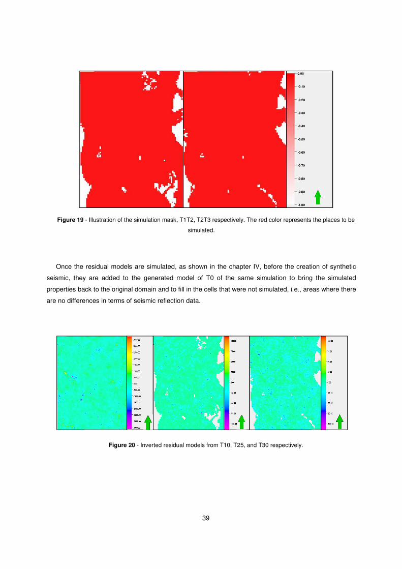
39
Figure 19 - Illustration of the simulation mask, T1T2, T2T3 respectively. The red color represents the places to be
simulated.
Once the residual models are simulated, as shown in the chapter IV, before the creation of synthetic
seismic, they are added to the generated model of T0 of the same simulation to bring the simulated
properties back to the original domain and to fill in the cells that were not simulated, i.e., areas where there
are no differences in terms of seismic reflection data.
Figure 20 - Inverted residual models from T10, T25, and T30 respectively.
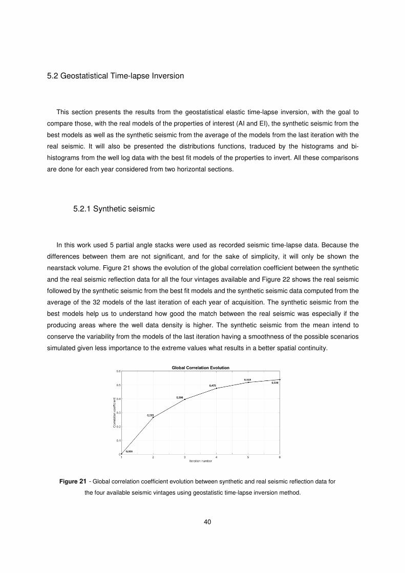
40
5.2 Geostatistical Time-lapse Inversion
This section presents the results from the geostatistical elastic time-lapse inversion, with the goal to
compare those, with the real models of the properties of interest (AI and EI), the synthetic seismic from the
best models as well as the synthetic seismic from the average of the models from the last iteration with the
real seismic. It will also be presented the distributions functions, traduced by the histograms and bi-
histograms from the well log data with the best fit models of the properties to invert. All these comparisons
are done for each year considered from two horizontal sections.
5.2.1 Synthetic seismic
In this work used 5 partial angle stacks were used as recorded seismic time-lapse data. Because the
differences between them are not significant, and for the sake of simplicity, it will only be shown the
nearstack volume. Figure 21 shows the evolution of the global correlation coefficient between the synthetic
and the real seismic reflection data for all the four vintages available and Figure 22 shows the real seismic
followed by the synthetic seismic from the best fit models and the synthetic seismic data computed from the
average of the 32 models of the last iteration of each year of acquisition. The synthetic seismic from the
best models help us to understand how good the match between the real seismic was especially if the
producing areas where the well data density is higher. The synthetic seismic from the mean intend to
conserve the variability from the models of the last iteration having a smoothness of the possible scenarios
simulated given less importance to the extreme values what results in a better spatial continuity.
Figure 21 - Global correlation coefficient evolution between synthetic and real seismic reflection data for
the four available seismic vintages using geostatistic time-lapse inversion method.
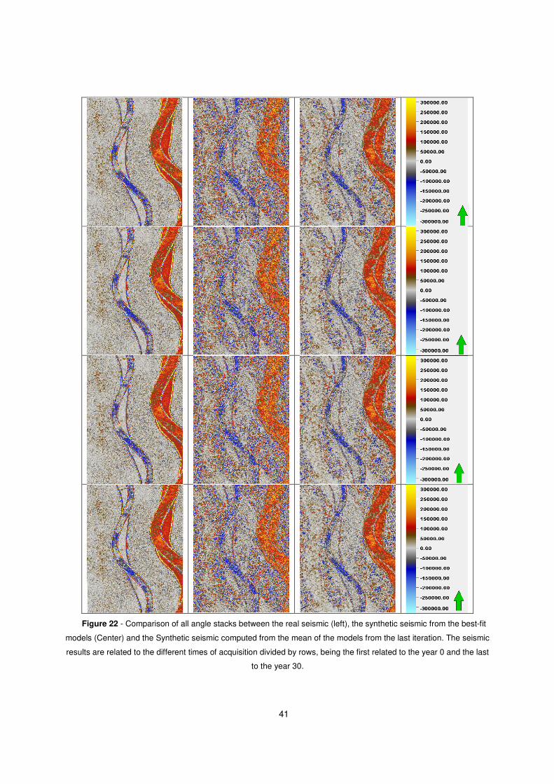
41
Figure 22 - Comparison of all angle stacks between the real seismic (left), the synthetic seismic from the best-fit
models (Center) and the Synthetic seismic computed from the mean of the models from the last iteration. The seismic
results are related to the different times of acquisition divided by rows, being the first related to the year 0 and the last
to the year 30.

42
5.2.2 Acoustic and Elastic Impedance Models
The acoustic and elastic impedances are the properties of interest inverted in this work, which were
simulated and co-simulated respectively, Figure 23 and Figure 24 show the comparison between the real
models of acoustic impedance and elastic impedance, respectively, with the best-fit inverted models of the
last iteration for these two properties. It is clear the presence of the fluvial channel of the left and the shapes
of the channels in the middle, a little less evident in the elastic impedance models.
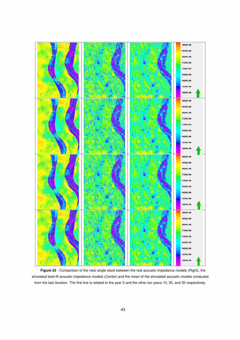
43
Figure 23 - Comparison of the near angle stack between the real acoustic impedance models (Right), the
simulated best-fit acoustic impedance models (Center) and the mean of the simulated acoustic models computed
from the last iteration. The first line is related to the year 0 and the other too years 10, 25, and 30 respectively.
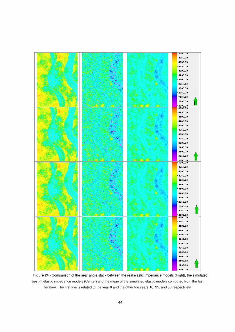
44
Figure 24 - Comparison of the near angle stack between the real elastic impedance models (Right), the simulated
best-fit elastic impedance models (Center) and the mean of the simulated elastic models computed from the last
iteration. The first line is related to the year 0 and the other too years 10, 25, and 30 respectively.

45
5.2.3 Histograms, Bi-plots and Statistics
This section introduces the results of this work regarding the statistical analysis from the best-fit models
illustrated previously. It comprises the probability distribution functions and the joint probability distribution
functions traduced by the histograms and the cross-plots between both properties, respectively, for each
acquisition time. Also the main statistics presented in the Table 3 and Table 4. These elements are very
important to retrieve from the well-log data as they allow us to evaluate, statistically, the global behavior of
the inverted model in to obtain a more reliable reproduction of the sub-surface geology. The joint and
marginal distributions in the bi-histograms are also very important to honor in the inverse models once, in
reservoir characterization, the extreme values of the properties need to be well reproduced. The Figures
25 and 26 represents the histograms from the well-log data and the best-fit models of acoustic and elastic
impedance respectively, and in the Figure 27 the cross-plots between the AI and EI of the well-log data and
the best-fit models.
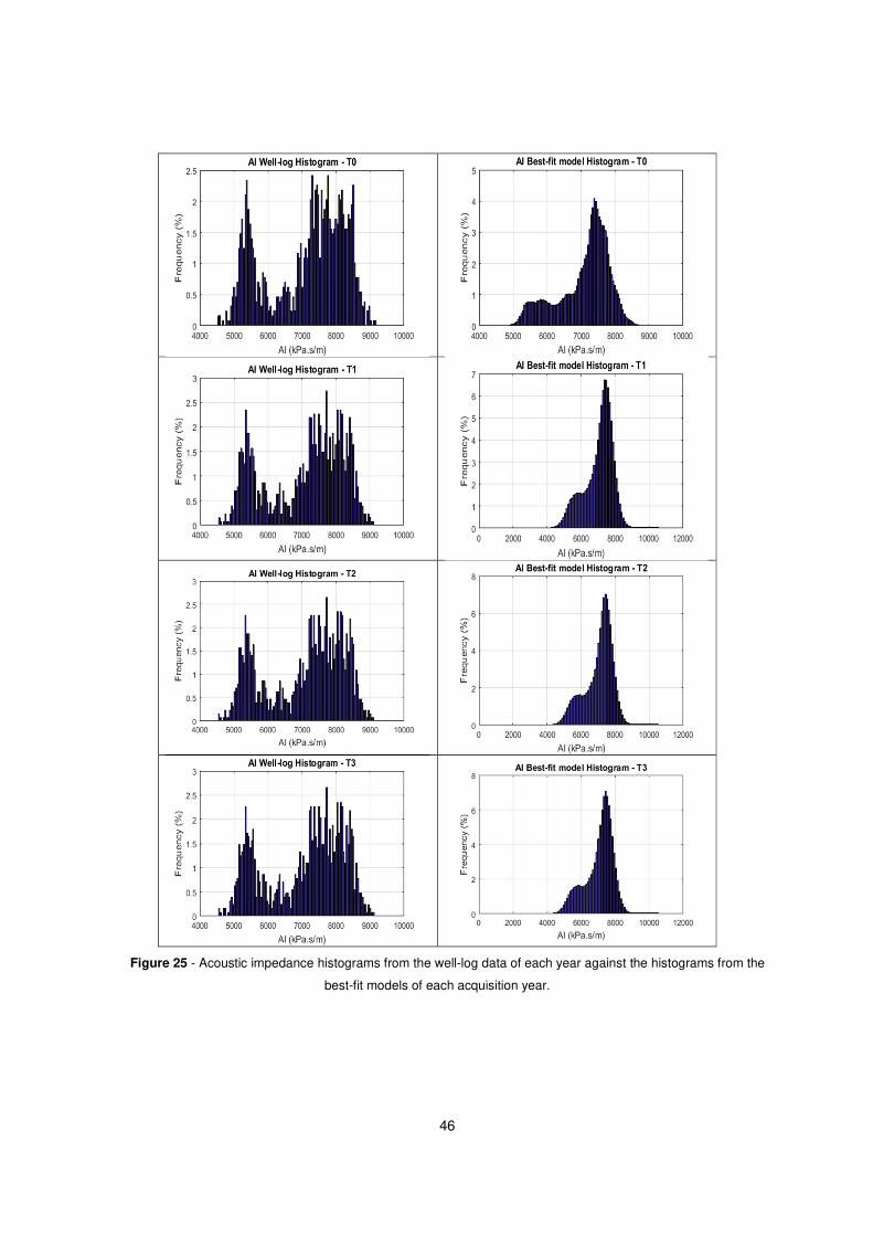
46
Figure 25 - Acoustic impedance histograms from the well-log data of each year against the histograms from the
best-fit models of each acquisition year.
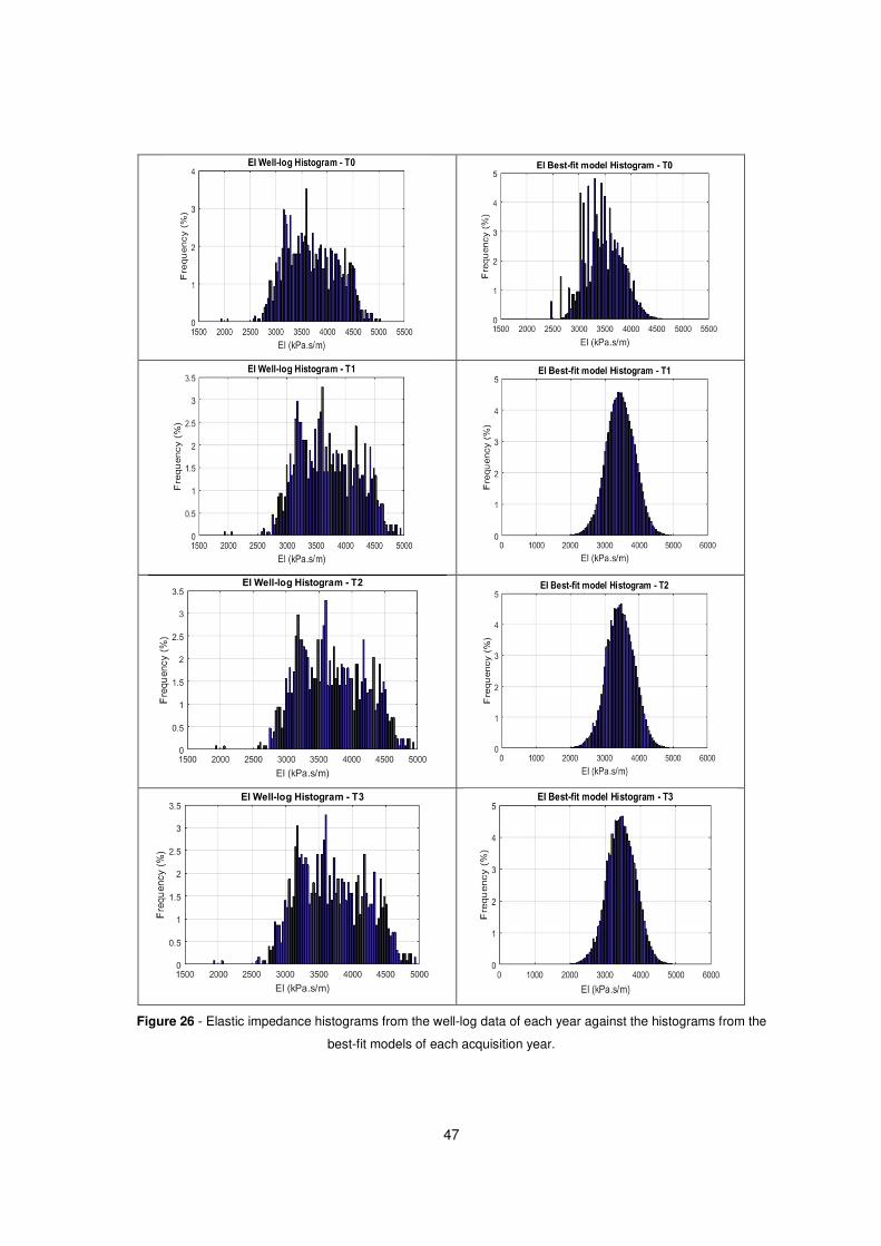
47
Figure 26 - Elastic impedance histograms from the well-log data of each year against the histograms from the
best-fit models of each acquisition year.
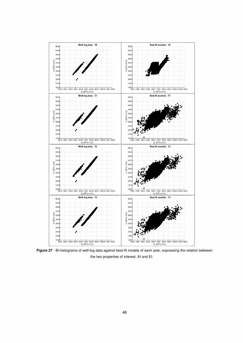
48
Figure 27 - Bi-histograms of well-log data against best-fit models of each year, expressing the relation between
the two properties of interest, AI and EI.
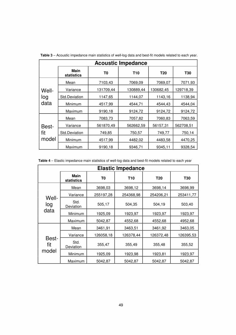
49
Table 3 – Acoustic impedance main statistics of well-log data and best-fit models related to each year.
Acoustic Impedance
Main
statistics T0 T10 T20 T30
Well-log data
Mean 7103,43 7069,09 7069,07 7071,93
Variance 131709,44 130889,44 130682,45 129718,39
Std.Deviation 1147,65 1144,07 1143,16 1138,94
Minimum 4517,99 4544,71 4544,43 4544,04
Maximum 9190,18 9124,72 9124,72 9124,72
Best-fit model
Mean 7083,73 7057,82 7060,83 7063,59
Variance 561870,49 562662,59 56157,31 562708,51
Std.Deviation 749,85 750,57 749,77 750,14
Minimum 4517,99 4482,02 4483,58 4470,25
Maximum 9190,18 9346,71 9345,11 9328,54
Table 4 – Elastic impedance main statistics of well-log data and best-fit models related to each year
Elastic Impedance
Main
statistics T0 T10 T20 T30
Well-log
data
Mean 3698,03 3698,12 3698,14 3698,99
Variance 255197,28 254368,98 254206,21 253411,77
Std. Deviation
505,17 504,35 504,19 503,40
Minimum 1925,09 1923,97 1923,97 1923,97
Maximum 5042,87 4552,68 4552,68 4952,68
Best-fit
model
Mean 3461,91 3463,51 3461,92 3463,05
Variance 126058,18 126378,44 126372,48 126395,53
Std. Deviation
355,47 355,49 355,48 355,52
Minimum 1925,09 1923,98 1923,81 1923,97
Maximum 5042,87 5042,87 5042,87 5042,87
50
5.3 Comparison between geostatistical elastic inversion and geostatistical time-lapse
inversion methodologies
This section, compares the seismic reflections and elastic models from the two geostatistical
methodologies used in this work. It aims show the efficiency of the proposed geostatistical time-lapse
seismic inversion methodology
5.3.1 Differences between seismic
In this section it is presented the comparison between seismic reflection data, and as explained before,
the 5 partial angle stacks used, did not show significant differences between then, therefore, after computing
synthetic seismic of the best-fit models in the geostatistical elastic inversion procedure and the synthetic
seismic from the mean of the best-fit models using the geostatistical time-lapse inversion, it was only used
the near stack to do the comparisons. As previously stated, using the synthetic seismic of the mean of the
best models helped us to grant a higher spatial continuity. Figure 28 illustrate the differences between real
seismic data and the synthetic seismic data from both methodologies.
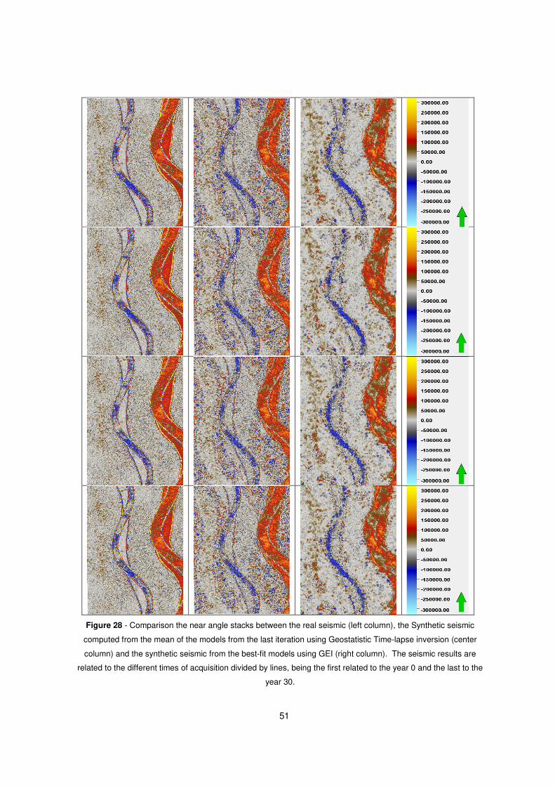
51
Figure 28 - Comparison the near angle stacks between the real seismic (left column), the Synthetic seismic
computed from the mean of the models from the last iteration using Geostatistic Time-lapse inversion (center
column) and the synthetic seismic from the best-fit models using GEI (right column). The seismic results are
related to the different times of acquisition divided by lines, being the first related to the year 0 and the last to the
year 30.
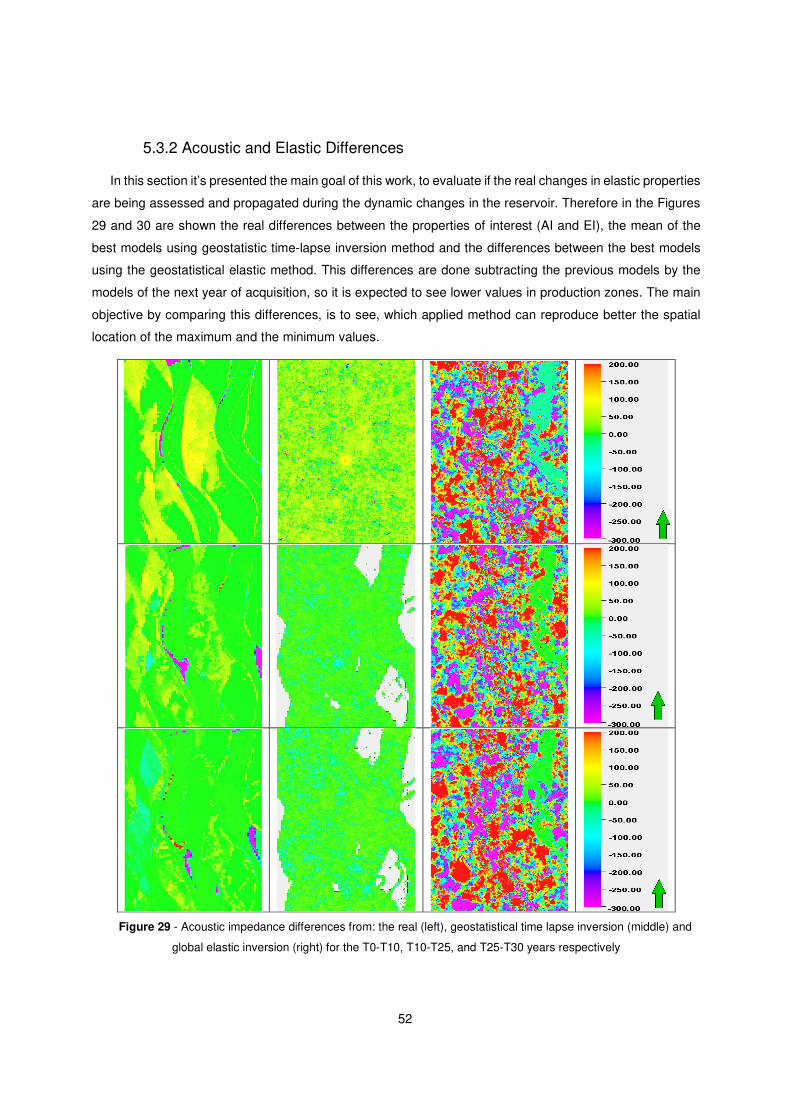
52
5.3.2 Acoustic and Elastic Differences
In this section it’s presented the main goal of this work, to evaluate if the real changes in elastic properties
are being assessed and propagated during the dynamic changes in the reservoir. Therefore in the Figures
29 and 30 are shown the real differences between the properties of interest (AI and EI), the mean of the
best models using geostatistic time-lapse inversion method and the differences between the best models
using the geostatistical elastic method. This differences are done subtracting the previous models by the
models of the next year of acquisition, so it is expected to see lower values in production zones. The main
objective by comparing this differences, is to see, which applied method can reproduce better the spatial
location of the maximum and the minimum values.
Figure 29 - Acoustic impedance differences from: the real (left), geostatistical time lapse inversion (middle) and
global elastic inversion (right) for the T0-T10, T10-T25, and T25-T30 years respectively
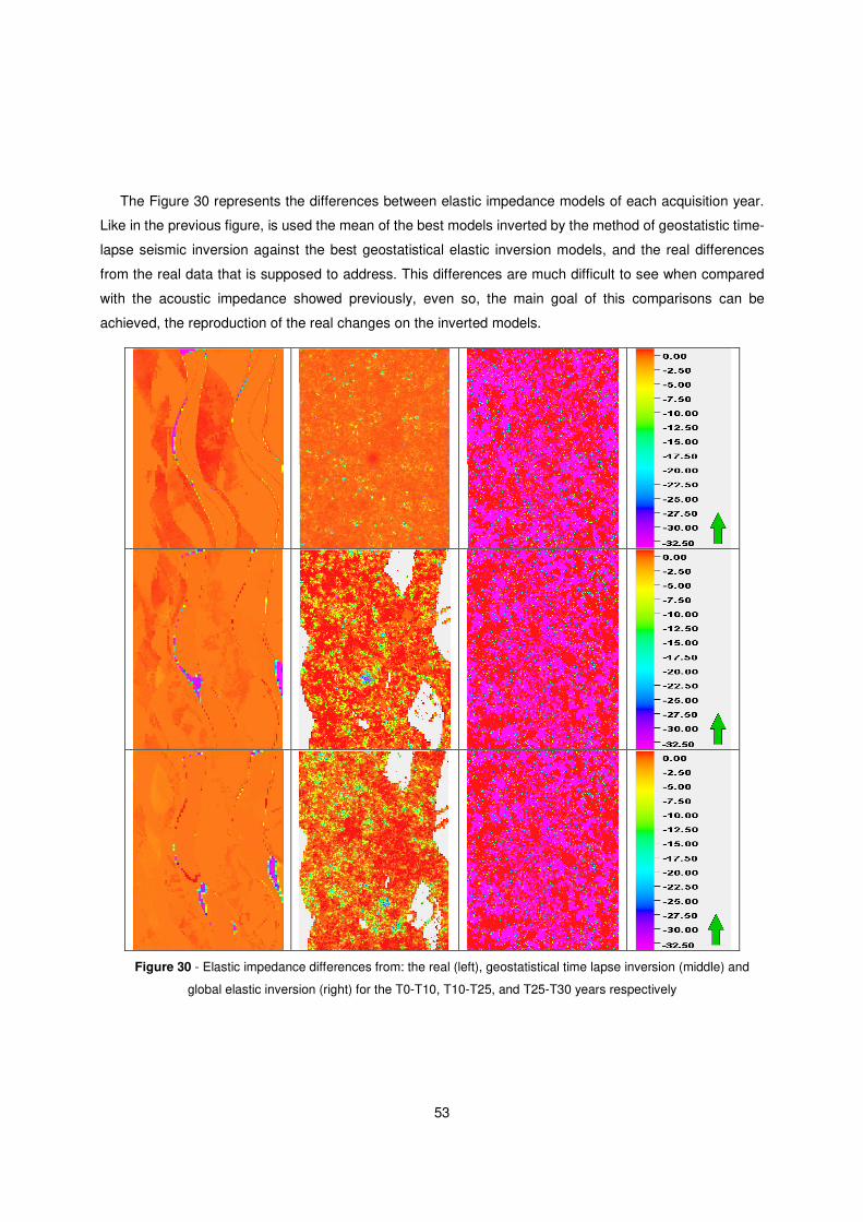
53
The Figure 30 represents the differences between elastic impedance models of each acquisition year.
Like in the previous figure, is used the mean of the best models inverted by the method of geostatistic time-
lapse seismic inversion against the best geostatistical elastic inversion models, and the real differences
from the real data that is supposed to address. This differences are much difficult to see when compared
with the acoustic impedance showed previously, even so, the main goal of this comparisons can be
achieved, the reproduction of the real changes on the inverted models.
Figure 30 - Elastic impedance differences from: the real (left), geostatistical time lapse inversion (middle) and
global elastic inversion (right) for the T0-T10, T10-T25, and T25-T30 years respectively

54
55
Chapter 6: Discussion, Conclusions and Future work
In this last chapter are discussed the results obtained using the geostatistical time-lapse inversion
compared to the real ones, and also the main results between the application of the proposed and the
geostatistical elastic inversion approaches. In the last part, are presented some final remarks of this work,
along with some suggestions associated with the future work in order to improve the results and the
efficiency of the proposed methodology.
The geostatistical time-lapse inversion methodology presented a reasonable global correlation
coefficient evolution (Figure 21) between the real seismic data and the synthetic seismic data of the inverted
elastic models. Although the convergence of the methodology was not high as we expected, this fact can
be explained regarding the main goal of this work, once we are inverting several seismic reflection data
acquisitions simultaneously, implying the integration of more set parameters within the objective function.
Nevertheless we obtained good representations of the synthetic seismic data (Figure 22) showing that, even
presenting some noise in the data, the main amplitude variations of the seismic are well illustrated by the
channels of the best-fit model. Computing the synthetic seismic data of the mean of the elastic models, lead
to a decreasing of the noise and consequently a better approximation to the real seismic data.
Attending to the obtained acoustic impedance models presented in Figures 23 it is possible to see that
the channel in the right side is very well retrieved comparing with the real one. The other channel in the
middle, is not so well reproduced like the previous one, fact that can be explain because of two reasons:
the low thickness of the channel, what reduces the seismic reflectivity area and the less well log data
available in that zone. Although these evidences, we can see its boundaries traduced by the lower acoustic
impedance values defining the main trend of the channel. The properties values on the zones between the
channels are not so closer to the real models, however the most important zones are the channels areas,
which correspond to the hydrocarbon accumulations when we are dealing with siliciclastic environments.
The same results are extended to the elastic impedance models (Figure 24), where we can still see the
channel in the right side but the channel in the middle is more difficult to distinguish, once this property is
harder to retrieve than the acoustic impedance in seismic inversion methodologies.
Playing a key role in what seismic inversion methodologies concern, the statistic elements and the
probability distribution functions are very important to be well reproduced in order to obtain more reliable
inverse models. As we can see from the histogram displayed in Figures 25 and 26 the main populations are
well reproduced comparing with those retrieved from well-log data for each property associated with each
acquisition year. One of the reasons that the population corresponding to the lower AI values are not so well
reproduced in the best-fit models histograms is that the well-log data presents less number of samples then
the best-fit models that comprise the values from all the simulation grid. Attending to the best-fit elastic
impedance histograms, it is important to highlight that the central class of values (around 3500 kPa.m/s) is
56
composed by the greatest number of samples, as in the case of well-log data histograms. The
representation of the joint probability distribution functions, traduced by the bi-plots (Figure 27), is also
satisfactory showing the trends of the relationship between the acoustic impedance against the elastic
impedance properties when compared with those retrieved from the available well-log data. In Tables 3 and
4, are presented the statistic concerning the well-log data and best-fit models related to each year. In general
the statistics of the inverse models are well reproduced compering with the well-log data, especially the
minimum and the maximum values of the data. For the other statistics to illustrate a better similarity, the
global convergence of the proposed methodology should present a higher value and the seismic data should
also be better inverted in all the simulation grid.
Moreover and in order to evaluate the performance of the proposed methodology, were also run a global
elastic inversion for each year separately conditioned by the same data set but directly inverting to the
properties themselves and not the elastic changes. The results obtained from both methodologies were
compared between them regarding the seismic reflection data and the properties differences between each
acquisition year.
Although the synthetic seismic is similar for both methods (Figure 28), the boundaries of the represented
channels are much better reproduced using the proposed methodology when compared with GEI. Also the
non-channel zones have more amplitude values close to the real seismic, as the GEI synthetic seismic have
more values close to zero and therefore different from the real one. Concerning the Figures 29 and 30, the
horizontal time-slices of elastic differences computed from the global elastic inversion present no spatial
continuity once the elastic difference values are not in the right locations in the simulation grid. Otherwise
the proposed method, even also do not show a good spatial continuity, we can verify that the range of elastic
changes values is honored, appearing in the right locations and within the property boundaries. The zones
where no elastic changes are noticed, are much better reproduced in the residual models of the proposed
methodology, giving us more reliable models regarding the study of the spatial uncertainty of elastic
differences. This better reproduction of elastic changes during all the years of production, can be explained
by the fact that the proposed methodology is able to simultaneously integrate the different seismic reflection
data, allowing the link between the differences from the previous and the next year of the acquisition time,
and also the fact of inverting directly to the elastic changes. Another great advantage when compared to
other seismic inversion algorithms (deterministic and Bayesian), is the possibility to presenting scenarios as
solutions, allowing a better assessment and quantification of the spatial uncertainty related with the geology
subsurface. All this advantages come with some limitations especially the computational costs and time
consuming once we are doing several seismic inversions simultaneously. Another fact that can greatly limit
the proposed methodology is associated to be a recent and in developing area and that need to have more
seismic acquisitions during the reservoir production stage. The fact that this methodology strongly depends
on the available 4D seismic data acquisition drives to a higher exploration costs and consequently the need
of a better improvement and knowledge regarding a study area. For these reasons, the development of this

57
proposed methodology would need more research and time investment to improve the optimization of the
workflow and the constraints in this approach.
As future work, we can go through this problem, integrating the petro-physical properties to build reliable
rock physic models, when we have more available wells-log data, in order to accurately estimate the elastic
changes of the properties and their dynamic behavior along the oil field life time.

59
References
Aanonsen, S. (2003). Effect of scale dependent data correlations in an integrated history matching loop
combining production data and 4D seismic data.
Avseth, P., Mukerji, T., & Mavko, G. (2010). Quantitative seismic interpretation: Applying rock physics tools
to reduce interpretation risk. Cambridge university press.
Avseth, Per, Mukerji, T., & Mayko, G. (2005). Quatitative Seimic Interpertation.
Azevedo, L. (2013). Geostatistical methods for integrating seismic reflection data into subsurface earth
models. Lisboa.
Bosch, M., Mukerji, T., & F.Gonzalez, E. (2010). Seismic inversion for reservoir properties combining
statistical rock physics and geostatistics : a review.
Buland, A., & El Ouair, Y. (2006). Bayesian time-laspe inversion.
Caetano, H. (2009). Integration of seismic information in seismic inversion.
Duijndam, A. (1988). Bayesian Estimation in Seimic Inversion. Part I : Principles Geophysical Prospecting.
Fatti, J., Smith, G., Vail, P., Strauss, P., & Levitt, P. (1994). Detection of gas in sandstone reservoirs using
AVO analysis: A 3-D seismic case history using the Geostack technicque. Geophysics, 59(9), 1362-
1376.
Francis, A. (2006). Understanding Stochastic Inversion : Part 1."First Break24 (November): 79-84.
Furre, A., Bakken, E., Kloy, T., & Nordby, L. (2006). Time-lapse seismic project integrating geophysics and
reservoir engineering.
Goovaerts, P. (1997). Geostatistics for Natural Resources and Evaluation. Geostatistics for Natural
Resources Evaluation. Oxford University Press.
Grana, D., Mukerji, T., Dvorkin, J., & Mavko, G. (n.d.). Stochastic Inversion of Faceis from Seismic Data
Based on Sequential Simulations and Probability Perturbation Method.
Horta, A., & Soares, A. (2010). Direct Sequential Co-simulation with Joint Probability Distributions.
Mathematical Geosciences.
Lafet, Y., Duboz, P., Deschizeaux, B., Lefeuvre, F., & Hubans, C. (2005). 4-D Stratigraphic Inversion of the
Girassol Field-Towards a Mora Quantitative Approach.
60
Lancaster , S., & Whitcombe, D. (2000). Fast track coloured inversion.
Landro, M., Veire, H., Duffaut, K., & Najjar, N. (2003). Discrimination between pressure and fluid saturation
changes from marine multicomponent time-lapse seismic data.
Lee, J., & Mukerji, T. (2012). The Stanford VI-E reservoir: A synthetic data set for joint seismic-EM time-
lapse monitoring algorithms.
Nunes, R., Schwedersky, G., Dillon, L., Guerreiro, L., Caetano, H., Maciel, C., & Leon, F. (2012).
Geostatistical Inversion of Prestack Seimic Data. .
Pereira, P. (2014). Inversão Geoestatística de Dados Sísmicos 3D Multi-distribuições Locais. Tese de
Mestrado em Engenharia Geologica, Universidade de Aveiro, Departamento de Geociencias ,
Aveiro.
R.O., L. (1979). Sysnthetic sonic logs-a process for startigraphic interpetation Geophysics.
Russel, B., & Hampson, D. (1991). Comparison of Poststack Seismic Inversion Methods.
Russel, B., & Toksoz, M. (1991). Comparison of poststack seismic inversion methods.
Russell, & H., B. (1988). Introduction to seismic inversion methods .
Sarkar, S., Gouveia, W., & Johnston, D. (2003). On the inversion of time-lapse seismic data.
Soares, A., Diet, J., & Guerreiro, L. (2007). Stochastic Inversion with a Global Perturbation Method.
Petroluem Geostatistics. Cascais.
Tarantola, A. (2005). Inverse Problem Theory.
Tompkins, Michael , J., Juan, L., Fernández, M., Alumbaugh, L., & Mukerji, T. (2011). Scalable Uncertainty
Estimation for NonLinear Inverse Problems Using Parameter Reductionn, Constraint Mapping, and
Geometric Sampling : Marine Controlled-Source. .
Ulrych, T. J., Sacchi, M. D., & Woodbury, A. (2001). A Bayes tour of inversion: A tutorial. Geophysics, 66(1),
55-69.

61

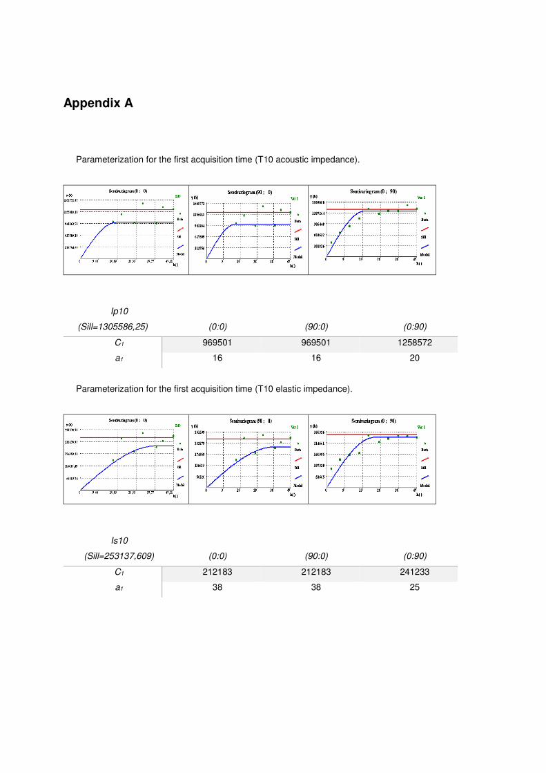
Appendix A
Parameterization for the first acquisition time (T10 acoustic impedance).
Ip10
(Sill=1305586,25)
(0:0)
(90:0)
(0:90)
C1 969501 969501 1258572
a1 16 16 20
Parameterization for the first acquisition time (T10 elastic impedance).
Is10
(Sill=253137,609)
(0:0)
(90:0)
(0:90)
C1 212183 212183 241233
a1 38 38 25
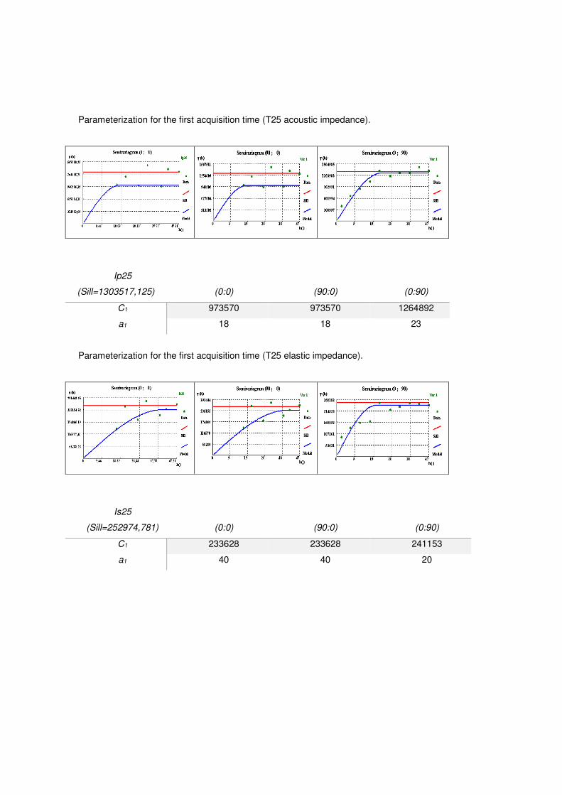
Parameterization for the first acquisition time (T25 acoustic impedance).
Ip25
(Sill=1303517,125)
(0:0)
(90:0)
(0:90)
C1 973570 973570 1264892
a1 18 18 23
Parameterization for the first acquisition time (T25 elastic impedance).
Is25
(Sill=252974,781)
(0:0)
(90:0)
(0:90)
C1 233628 233628 241153
a1 40 40 20
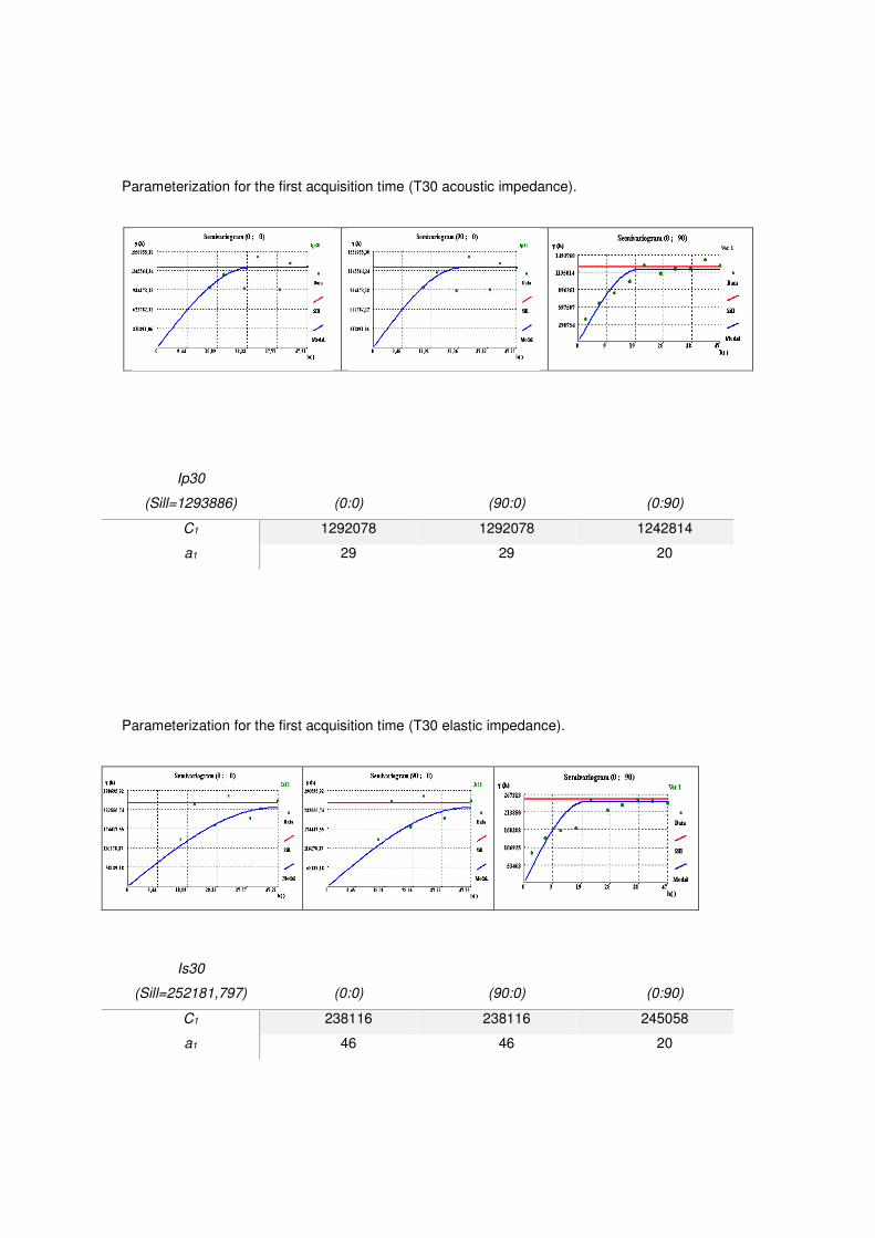
Parameterization for the first acquisition time (T30 acoustic impedance).
Parameterization for the first acquisition time (T30 elastic impedance).
Is30
(Sill=252181,797)
(0:0)
(90:0)
(0:90)
C1 238116 238116 245058
a1 46 46 20
Ip30
(Sill=1293886)
(0:0)
(90:0)
(0:90)
C1 1292078 1292078 1242814
a1 29 29 20


