
Geog 463: GIS Workshop
May 17, 2006
Exploratory Spatial Data Analysis

Outlines
I. Fundamentals of ESDA1. What is Exploratory Spatial Data Analysis (ESDA)?2. ESDA basics
II. Techniques of ESDA with focus on area-class data3. ESDA for describing non-spatial properties of attribute4. ESDA for describing spatial properties of attribute
III. Applications of ESDA5. Gallery of implemented ESDA systems

I. Fundamentals of ESDA

1. What is ESDA?
• Exploratory Spatial Data Analysis (ESDA)
• Exploratory Data Analysis (EDA)
• EDA and statistics
• EDA and visualization
• EDA and cartographic visualization

Exploratory Spatial Data Analysis
• Extension of exploratory data analysis (EDA) to detect spatial properties of data
• EDA – consists of a collection of descriptive and graphical
statistical tools – intended to discover patterns in data and suggest
hypotheses – by imposing as little prior structure as possible
• ESDA links numerical and graphical procedures with the map

Exploratory Data Analysis
• Aimed at (1) pattern detection (2) hypothesis formulation (3) model assessment
• Use of graphical and visual methods (e.g. Box plot); Use of numerical techniques that are statistically robust (e.g. P-value)
• Emphasis on descriptive methods rather than formal hypothesis testing
• Exploratory in that it cannot explain the patterns it reveals
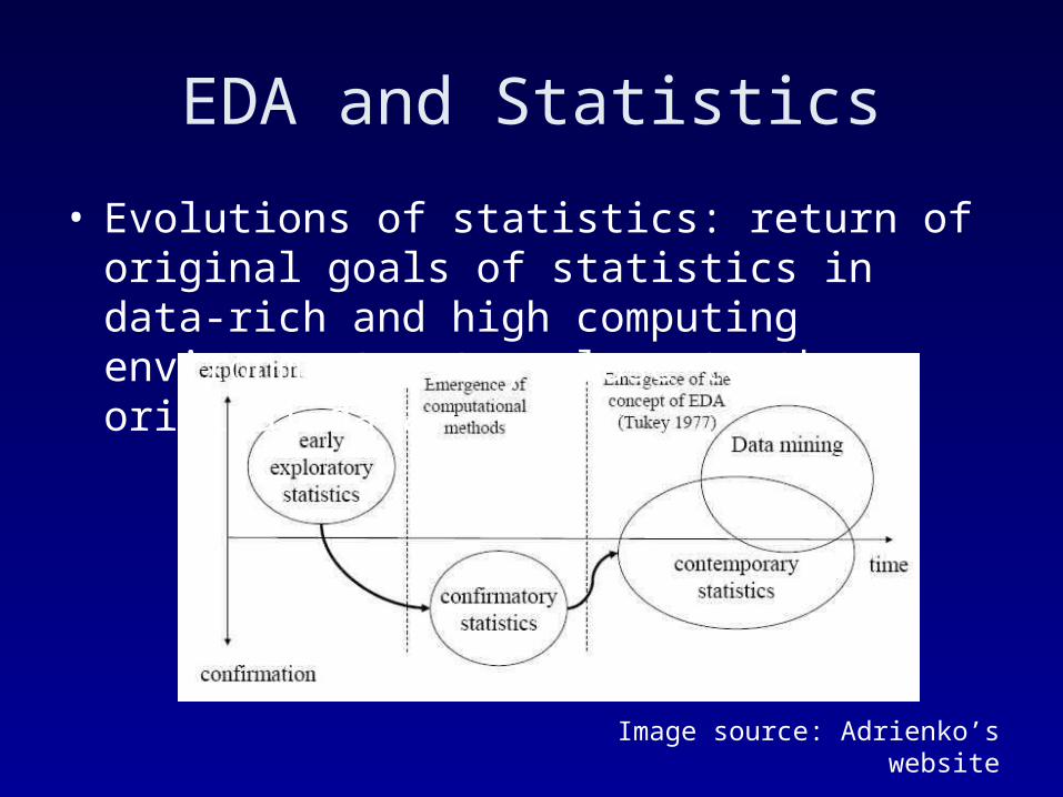
EDA and Statistics
• Evolutions of statistics: return of original goals of statistics in data-rich and high computing environment; stay close to the original data
Image source: Adrienko’s website

EDA and Visualization
• By its very nature the main role of EDA is to open-mindedly explore, and graphics gives the analysts unparalleled power to do so
• The greatest value of a picture is when it forces us to notice what we never expected to see
– John W. Tukey

EDA and Cartographic Visualization
• Emphasis on the role of highly interactive maps in individual and small group efforts at hypothesis generation, data analysis, and decision-support
• Contrast with static paper maps

infected water pump?infected water pump?
Dr. John Snow: Dr. John Snow: Investigation of Investigation of
deaths from choleradeaths from choleraLondon, September 1854London, September 1854
death locationsdeath locations
spatial clusterspatial cluster
A good data representation is the key to solving the problem
Early examples of ESDA
2. ESDA Basics
• Visual tools for non-spatial analyses– Univariate– Multivariate
• Visual tools for spatial analyses– First-order properties– Second-order properties
• Brushing & Linking

Visual tool for non-spatial analyses
• Univariate– Histogram– Box plot
• Multivariate– Scatter plot– Parallel coordinates plot

Distribution of attribute values within a range
Dot plot
Dispersion graph
Histogram
Histogram, box plot
Box plot
Distribution of attribute values at y-axis given categorical variables at x-axis

Scatter plot
Scatter plot: shows how two attributes are related Scatter plot matrix:
shows how a set of two attributes are related

Parallel coordinates plot
Parallel coordinates plot: object characteristics profiles; relationships
between attributes (look at line slopes)

Visual tools for spatial analyses
• First order properties– Tools for exploring general trends
• Spatially lagged boxplot• Kernel estimation
• Second order properties– Tools for exploring spatial autocorrelation
• Moran plot

Spatially lagged boxplot
• Boxplot in which the categorical variable is spatial lag order (as defined by spatial weight matrix)
• After the user has selected an origin zone, a sequence of box plots (one for each lag order) is generated at increasing distance from the origin zone up to a user specified maximum

Wise et al 1998
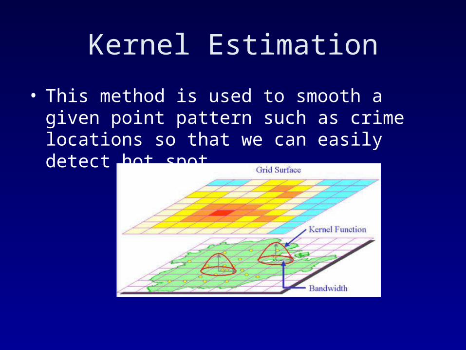
Kernel Estimation
• This method is used to smooth a given point pattern such as crime locations so that we can easily detect hot spot.


Moran plot
• A plot of attribute value on the vertical axis against the average of the attribute values in the adjacent areas using spatial weight matrix
• A scatter of values sloping upward to the right is indicative of positive autocorrelation
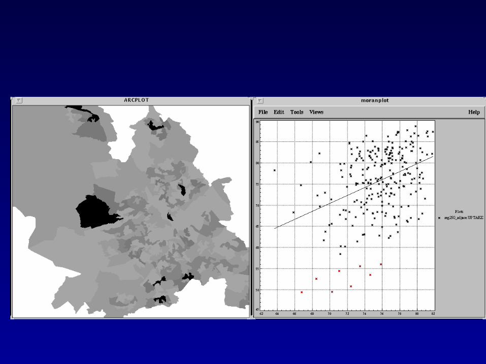
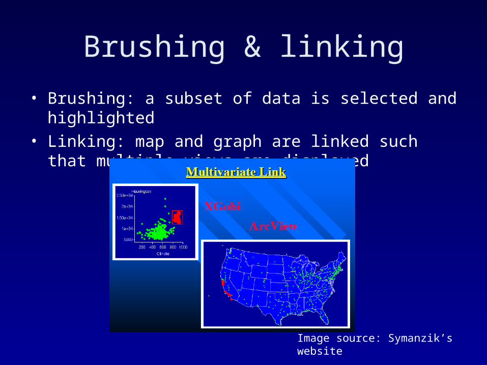
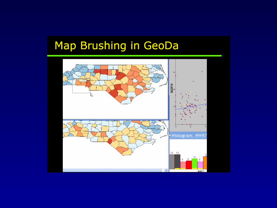
Brushing & linking
• Brushing: a subset of data is selected and highlighted• Linking: map and graph are linked such that multiple
views are displayed
Image source: Symanzik’s website

II. Techniques of ESDA

3. ESDA for describing non-spatial properties of attribute
• Median– Measure of the center of the distribution of attribute values– ESDA queries: which are the areas with attribute values above
(below) the median?
• Quartile and inter-quartile spread– Measure of spread of values about the median– ESDA queries: which are the areas that lie in the upper (lower)
quartile?
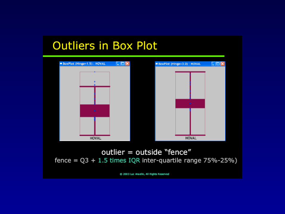
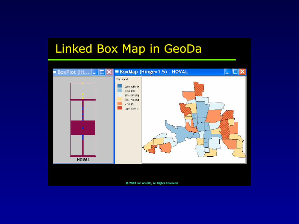
• Box plots– Graphical summary of the distribution of attribute values– ESDA queries: where do cases that lie in specific parts of the
boxplot occur on the map? Where are the outlier cases located on the map?

4. ESDA for describing spatial properties of attribute
• Smoothing
• Identifying trends and gradients on the map
• Spatial autocorrelation
• Detecting spatial outliers

Smoothing
• Smoothing may help to reveal the presence of general patterns that are unclear from the mosaic of values
• ESDA techniques: spatial averaging – take the attribute value of an area and its neighbors and average them; repeat for each area

Identifying trends and gradients on the map
• Are there any general trends or gradients in the map distribution of values?
• ESDA techniques include– Kernel estimation– Taking transects through the data and plotting
with attribute value on vertical axis and spatial location on horizontal axis
– Spatially lagged boxplot with lag order specified with respect to a particular area or zone

Spatial autocorrelation
• Propensity for attribute values in neighboring areas to be similar
• ESDA techniques include– Moran plot

Detecting spatial outliers
• An individual attribute value is not necessarily extreme in the distributional sense but is extreme in terms of the attribute values in adjacent areas
• ESDA technique: run a linear squares regression on the Moran plot, and select cases significantly deviated from the regression line


III. Applications of ESDA

5. Gallery of ESDA systems
• GeoDa– https://www.geoda.uiuc.edu/default.php
• CommonGIS– http://www.commongis.com/


Interactive map symbolization in CommonGIS
West-to-east increase
Clusters of low values around Porto and Lisboa
One more cluster of low values
Coast-inland contrast
Clusters of high values in central-east
By moving the slider, we see more patterns and gain more understanding of value distribution
Porto
Lisboa

Link between information visualization techniques and maps
Map and scatter plot: the same techniqueMap and dot plot; each district shown on the map is also represented by a dot
Map
Dot plot
A district pointed on the map with the mouse is simultaneously
highlighted on the map and the plot

Using Cumulative CurvesSome statistics about the result:
In these areas over 7.82% people have high school education. Here lives 33.1%
of the total country’s population.
In the most part of Portugal (coloured in blue) the proportion of people having high school education is below 4.67. However, on this large territory only one third of the country’s population lives.

is simultaneously highlighted here,
Focusing & multiple views
An object pointed on
the map with the mouse and here,
and here,
but not here: this is an aggregated view that does
not show individual objects

Focusing and Visual Comparison on Other Map Types
OutlierMaximum represented value
Value to compare withMinimum value

Spatial Distribution of EventsThe small circles represent the earthquakes that occurred in Western Turkey and the neighbourhood between 01.01.1976 and 30.12.1999
By applying the temporal filter, we can investigate the spatial distribution on any time interval
Here we see only the earthquakes that occurred during 30 days from 15.05.1977 to 13.06.1977

Progress of Spatial Patterns over Time
Map animation allows us to see how the spatial distribution of events and their characteristics evolve over time
15.05.1977 - 13.06.1977 25.05.1977 - 23.06.1977 04.06.1977 - 03.07.1977
14.06.1977 - 13.07.1977 24.06.1977 - 23.07.1977 04.07.1977 - 02.08.1977
Each animation frame in this example covers 30-days time interval. The step between the frames is 10 days. Hence, there is 20 days overlap between the adjacent frames.

Exploration of Behaviors
The value flow symbols show us the evolution of attribute values
(behavior) at each location.
Unfortunately, symbol overlapping creates significant inconveniences, and zooming does not always help

Data Transformations for Behavior Exploration
As with time maps, various data transformations can be applied to value flow maps.
Here we have applied the comparison to the mean: the values for each moment are replaced by their differences to the country’s mean at the same moment. Yellow colour corresponds to positive differences, and
blue – to negative. We have received a rather clear spatial pattern.

Due to Due to direct manipulationdirect manipulation computer computer screens will play no less revolutionary screens will play no less revolutionary
role for data exploration than the role for data exploration than the invention of Cartesian coordinatesinvention of Cartesian coordinates
W.Cleveland 1993
High interactivity
Enabling multiple complementary views
allow the user ... to “see” data from multiple perspectives
A.MacEachren and M.-J. Kraak 1997
Summary: Characteristics of ESDA

Summary: Methods of ESDA
• Manipulating data• Varying the symbolization• Manipulating the user’s viewpoint• Highlighting portions of a data set• Multiple view• Animation• Linking maps with other forms of display• Access to miscellaneous resources• Automatic map interpretation (i.e. data mining)
From Slocum et al 2005

Discussion questions
• Assess the value of ESDA techniques in analyzing any geographical data with which you are familiar
• Discuss the strengths and weakness of current GIS software for undertaking ESDA

Value of ESDA in analyzing spatial data
• Help reveal unknown pattern that couldn’t be revealed without multiple views or other ESDA mechanisms– Moran plot for identifying spatial outlier– Parallel coordinate plot for looking at the data distribution of a particular
record relative to other records
• Help create a map that fits into user’s need– Can select a subset of data related to map purpose (user interaction)
• Help avoid jumping to the conclusion with a single thematic map or solely based on visual impact– By letting users explore the consequence of different map symbolization
or map design– By letting users determine whether the pattern is unusual (use of
statistics)
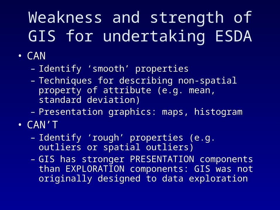
Weakness and strength of GIS for undertaking ESDA
• CAN– Identify ‘smooth’ properties– Techniques for describing non-spatial property of
attribute (e.g. mean, standard deviation)– Presentation graphics: maps, histogram
• CAN’T – Identify ‘rough’ properties (e.g. outliers or spatial
outliers)– GIS has stronger PRESENTATION components than
EXPLORATION components: GIS was not originally designed to data exploration
References• Anselin, 1998, Geocomputation: A Primer, pp. 77-94• Anselin, 2005, GeoDa workbook• Haining & Wise, 1998, Providing scientific visualization for spatial
data analysis: criteria and assessment of SAGE, retrieved from http://www.ersa.org/ersaconfs/ersa98/papers/409.pdf
• Haining & Wise, 2000, GISCC Unit 128• Slocum et al, 2005, Thematic Cartography and Geographic
Visualization, pp. 389-405• Wise et al, 1998, The role of visualization in the exploratory spatial
data analysis of area-based data, retrieved from http://www.geocomputation.org/1998/81/gc_81.htm
• Adrienko’s website: http://www.ais.fraunhofer.de/and/– One of authors of CommonGIS
• Symanzik’s website: http://www.math.usu.edu/~symanzik/– One of authors of xGobi


